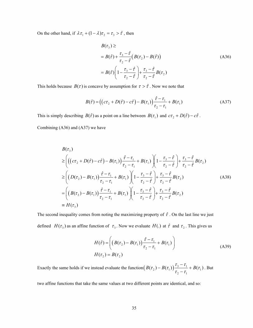
1 Strategic safety stocks in supply chains with capacity constraints May 2008, revised January 2009 Tor Schoenmeyr • Stephen C. Graves Optisolar, Inc. 31302 Huntwood Avenue, Hayward, CA 94544, [email protected]Leaders for Manufacturing Program and A. P. Sloan School of Management, Massachusetts Institute of Technology, Cambridge, Massachusetts 02139-4307, [email protected]We generalize the guaranteed-service (GS) model for multi-echelon safety stock placement to include capacity constraints. We first develop an extension of the single-stage base-stock model to include a capacity constraint. We then use this result to model a multi-stage system with a base-stock operating policy. We establish that we can adapt the existing algorithms for the un- constrained case to solve for the safety stocks in a capacitated system. We then consider a multi- stage system in which stages censor their orders, based on their capacity limits. Again we analytically characterize the necessary base stock levels, and develop an extension to the existing dynamic programming algorithms to find the optimal base stock levels and safety stocks. The censored order policy leads to a better solution compared to that for the base-stock policy. Indeed, we find that the total holding costs for the censored order policy can be less than that for the corresponding base-stock system without capacity constraints. Subject classifications: Inventory/production: Multi-echelon; policies. Manufacturing: Strategy.
Transcript
1
Strategic safety stocks in supply chains with capacity constraints
May 2008, revised January 2009 Tor Schoenmeyr • Stephen C. Graves
Optisolar, Inc. 31302 Huntwood Avenue, Hayward, CA 94544, [email protected] Leaders for Manufacturing Program and A. P. Sloan School of Management,
Massachusetts Institute of Technology, Cambridge, Massachusetts 02139-4307, [email protected] We generalize the guaranteed-service (GS) model for multi-echelon safety stock placement to include capacity constraints. We first develop an extension of the single-stage base-stock model to include a capacity constraint. We then use this result to model a multi-stage system with a base-stock operating policy. We establish that we can adapt the existing algorithms for the un-constrained case to solve for the safety stocks in a capacitated system. We then consider a multi-stage system in which stages censor their orders, based on their capacity limits. Again we analytically characterize the necessary base stock levels, and develop an extension to the existing dynamic programming algorithms to find the optimal base stock levels and safety stocks. The censored order policy leads to a better solution compared to that for the base-stock policy. Indeed, we find that the total holding costs for the censored order policy can be less than that for the corresponding base-stock system without capacity constraints. Subject classifications: Inventory/production: Multi-echelon; policies. Manufacturing: Strategy.
2
Strategic safety stocks in supply chains with capacity constraints
May 2008, revised January 2009 Tor Schoenmeyr • Stephen C. Graves
Optisolar, Inc. 31302 Huntwood Avenue, Hayward, CA 94544, [email protected] Leaders for Manufacturing Program and A. P. Sloan School of Management,
Massachusetts Institute of Technology, Cambridge, Massachusetts 02139-4307, [email protected]
We generalize the guaranteed-service (GS) model for multi-echelon safety stock placement to
include capacity constraints. We first develop an extension of the single-stage base-stock model
to include a capacity constraint. We then use this result to model a multi-stage system with a
base-stock operating policy. We establish that we can adapt the existing algorithms for the un-
constrained case to solve for the safety stocks in a capacitated system. We then consider a multi-
stage system in which stages censor their orders, based on their capacity limits. Again we
analytically characterize the necessary base stock levels, and develop an extension to the existing
dynamic programming algorithms to find the optimal base stock levels and safety stocks. The
censored order policy leads to a better solution compared to that for the base-stock policy.
Indeed, we find that the total holding costs for the censored order policy can be less than that for
the corresponding base-stock system without capacity constraints.
1. Introduction A central question in supply chain management is how to coordinate activities and inventories
over a large number of stages and locations, while providing a high level of service to end-item
customers. Simpson (1958) found that if the individual stages in a serial-system supply chain
operate according to base stock policies with service guarantees, then the optimal safety stock
strategy is to concentrate inventory to certain key locations, effectively decoupling different parts
3
of the supply chain. Once the optimal safety stock strategy has been determined, each stage of the
supply chain can operate independently, providing guaranteed service to its downstream
customer, and operating according to a simple base stock policy, with a minimum need for
communication and coordination between different parts of the supply chain. Graves and Willems
(2003) term this framework for supply chain management as the guaranteed service (GS) model.
To our knowledge, all published work on the GS model assumes unlimited capacity for
processing and inventory storage at each stage. In reality, there are often limits to the quantity of
goods that can be transported, processed or stored in a given time frame. If a stage is unable to
process a large order in a short period of time, then this may cause delays and stock-outs that are
not anticipated by existing theoretical models.
The intent of this paper is to extend the GS model for the optimal placement of safety
stock inventory to supply chains with capacity constraints. In particular we strive to develop
models and algorithms that have the potential to determine safety stocks in real-world supply
chains. We assert that the paper makes three contributions.
First we determine for a single-stage capacitated system the base-stock level that is
required to provide guaranteed service, assuming bounded demand. This is a generalization of
Kimball’s classic single-stage base-stock model (original manuscript 1955, reprinted in 1988) to
account for a capacity constraint.
Second, we use the single-stage model to model a supply chain, namely a multi-stage
network, where each stage can have a capacity constraint and where we assume that each stage
operates with a base-stock policy. With the assumption of a concave demand bound, the optimal
placement of safety stocks for a serial-system supply chain satisfies the all-or-nothing property:
that is, each stage either holds a decoupling safety stock or no safety stock. We then establish for
networks with spanning tree topologies that we can directly apply the efficient safety-stock
optimization methods developed for uncapacitated supply chains to the safety-stock optimization
problem for capacitated supply chains.
4
Third, we analyze a modification of the base-stock policy, in which a node propagates an
order which is the lesser of its capacity and the order it receives (plus extra quantities to “catch
up”, as necessary). We refer to this as the “censored” ordering policy. We show again that the all-
or-nothing property holds for serial systems. We also show that we can optimize the safety stock
inventory in supply chains with censored ordering and capacity constraints, with small
modifications to the Graves-Willems’ dynamic programming method. We find that the inventory
holding costs for the censored ordering policy are less than for the original base-stock policy, and
sometimes even less than that for the corresponding system without capacity constraints.
Moreover, for the censored policy the orders still depend only on local information.
This paper consists of six sections. In the remainder of this section, we provide a brief
review of related literature. In §2, we generalize the base-stock model of Kimball (1988) and
Simpson (1958) to include a capacity constraint in a single-stage setting. In §3, we consider
optimization of a supply chain with a base-stock policy and potentially any number of capacity
constraints. In particular, we find that the optimization procedures and structural results identified
by Simpson (1958) and Graves and Willems (2000) carry over to this setting. In §4, we analyze
what happens if each stage modifies its order based on its capacity constraint, i.e., censors the
order. We find that the structural properties and optimization methods carry over to this setting
as well. In §5, we perform a numerical experiment to examine the structure and performance of
these policies. We conclude the paper with a discussion on our findings and suggestions for
possible future work in §6.
Literature Review
For a review of work on GS models we cite the overview articles of Inderfurth (1991),
Diks et al. (1996) and Graves and Willems (2003). Graves and Willems (2000) extend Simpson's
work to supply chains with spanning tree topology, and formulate an efficient dynamic
programming algorithm. Optimizing general networks is an NP-hard problem (Lesnaia et al.
2005); nevertheless, Humair and Willems (2006, 2008) have developed very effective algorithms
5
for optimizing the safety stocks in large-scale real-world supply chains. We also note that the GS
framework has been deployed successfully in industry (e.g., Billington et al 2004, Willems 2008).
There is a somewhat larger literature examining capacity constraints for stochastic
service (SS) models, in which the delivery or service time between stages can vary depending
upon the material availability at the supply stage. The main focus for much of this literature has
been to characterize the structure of the optimal ordering policy. Gallego and Scheller-Wolf
(2000) examine a single stage system with fixed ordering costs and capacity constraints, and find
that the optimal policy takes an (s,S) form. Gallego and Toktay (2004) also consider a single-
stage system under the assumption that all orders are full capacity orders, and show that the
optimal policy is a threshold policy.
For multi-stage systems, Speck and van der Wal (1991) show by example that the
echelon-based ordering policy of Clark and Scarf (1960) is generally not optimal in a two-stage
serial system with capacity constraints. Parker and Kapuscinski (2004) also analyze a two-stage
serial system, and show that a modified echelon base stock (MEBS) policy is optimal, when the
tightest capacity constraint is at the downstream stage and there is no lead-time at the upstream
stage. For these specific assumptions the MEBS policy is the same as the censored ordering
policy that we propose and analyze. However, for serial systems with more than two stages and
non-zero lead-times, these policies will differ. In particular, the MEBS policy is a modification to
an echelon base-stock policy; as such, an upstream stage will see the end-item demand and will
replenish accordingly, subject to a possible capacity constraint at the stage. Our censored
ordering policy is a modification to a local base-stock policy, whereby an upstream stage only
sees the order from its adjacent downstream stage. Furthermore, at each capacitated stage, the
stage orders the lesser of its capacity and shortfall between its inventory position and its local
base-stock level. As such, the order signal gets censored at each stage as it is passed upstream.
Glasserman and Tayur (1994) consider the stability properties of multi-echelon systems
with capacity constraints. They find that inventories and back-logs are stable (i.e., they converge
6
to unique stationary distributions from any initial state) if the mean demand is less than the
capacity constraint. In subsequent papers, Glasserman and Tayur assume that an echelon-base
stock policy is used in a multi-echelon system, and find optimal order points using simulation and
perturbation analysis (Glasserman and Tayur, 1995), and analytical approximations (Glasserman
and Tayur, 1996).
Gupta and Selvaraju (2006) develop an approximation for analyzing a serial system as a
queueing network, where the stages have exponentially distributed service times and operate
according to echelon base-stock policies. In this way, they can characterize and optimize a two-
stage system with capacity constraints. This approach is computationally costly for larger
systems, for which Gupta and Selvaraju propose some approximations.
A markedly different approach is taken by Bertsimas and Thiele (2004, 2006), who show
that capacity constraints can be incorporated into a tractable, robust optimization problem. This
approach can handle general networks, and uses echelon policies as in the Clark and Scarf (1960)
model. A similarity between the robust optimization approach and ours is that there is no need to
specify a probability distribution for demand. However, our work differs from all of the
aforementioned work in that we consider local base-stock ordering policies, and, as mentioned,
guaranteed service constraints rather than back-order costs and stochastic service. Moreover, we
will show that existing optimization algorithms (Graves and Willems, 2000) can be generalized to
handle capacity constraints. In practice, these methods are fast enough to handle systems with
thousands of stages.
2. Single stage model In this section we generalize the single-stage model originally developed by Kimball
(1988) and Simpson (1958) to include a capacity constraint. A stage represents a processing
activity that requires one or more inputs and that converts these inputs into an output product or
final good. The output can be stored as inventory at the stage, and is used to meet demand from
7
multiple customers or as input into downstream stages. The stage might represent the
procurement of a raw material, or the production of a component, or the manufacture of a
subassembly, or the assembly and test of a finished good, or the transportation of a finished
product from a distribution center to a warehouse.
We let ( )d t denote the demand in period t. We assume that the stage provides the same
guaranteed service time S to each of its customers; this means that the stage guarantees that it will
satisfy the demand ( )d t by time t + S, where S is a non-negative integer.
We also assume that the suppliers to the stage provide a guaranteed service time, which
we denote by SI for the inbound service time. Thus, for an order placed at time t, the suppliers
will deliver their inputs to the stage at time t + SI.
The stage has a capacity limit c: each period the stage can release into its process any
amount up to the capacity limit of c, assuming that all of the inputs are on hand. We assume a
deterministic lead-time T equal to the time between when the process starts and when the process
completes and the inventory is available to serve demand. The lead-time represents any fixed
processing time at the stage (and does not include any time waiting for input; see below). For
instance, for a transportation stage, the lead-time is the time to transport inventory (say) from a
manufacturing plant to a distant warehouse; for a manufacturing stage, the lead-time might be a
batch processing time. The lead-time can be zero, if there is no fixed processing time.
The stage operates with a periodic review base-stock replenishment policy with a review
period being one time unit (e.g., one day). The timing of events is as assumed by Kimball (1988)
and Simpson (1958). In each period t, the stage first observes its demand ( )d t and then places
an order on each of its upstream suppliers. The stage then receives the earlier order placed at
time t – SI from each of the upstream suppliers; decides the quantity to release into its process;
and completes the process on the release quantity from time t – T and places this quantity into its
inventory. Finally the stage serves the demand from period t – S, namely ( )d t S− .
8
For the base-stock policy without a capacity constraint, each period the stage places an
order, equal to ( )d t , on its upstream suppliers. When these inputs are received at time t + SI, the
stage will then initiate production of ( )d t units; that is, the release quantity at time t + SI is
( )d t , which will complete the process and be placed in inventory at time t + SI + T.
We now adapt this policy to account for a capacity constraint. We again assume
that each period the stage places an order, equal to ( )d t , on each of its upstream suppliers.
When the stage receives these inputs at time t + SI, it places the supplies into an internal queue;
the stage will then process as much of the internal queue as possible, subject to its capacity
constraint. When the constraint is binding, the stage will release less than ( )d t at time t + SI ,
and the delayed production (in the form of the internal queue) is carried over until the next time
period. We illustrate the envisioned arrangement in Figure 1.
Figure 1: Overview of a single-stage system
We denote the production release at time t by ( )R t . With capacity constraints, we have
( ) min( , ( ) ( 1))R t c d t SI IQ t= − + − , (1)
where ( )IQ t is the internal queue, given by the equation:
( ) ( 1) ( ) ( )IQ t IQ t d t SI R t= − + − − . (2)
The balance equation for the final-good inventory ( )I t at the stage is now:
9
( ) ( ) ( ) ( )1I t I t R t T d t S= − + − − − . (3)
Combining (2) and (3) we have
( ) ( ) ( ) ( ) ( ) ( )1 1I t IQ t T I t IQ t T d t T SI d t S+ − = − + − − + − − − − . (4)
If the system starts at time t = 0 with ( ) ( ) ( )0, 0, for 0 and 0d t IQ t t I B= = ≤ = , where B is
the base-stock level, then for suitably large t we can write the inventory as:
( ) ( ) ( ),I t B d t T SI t S IQ t T= − − − − − − (5)
where we define the notation
( )
( )
( )
1
1
for
, 0 for
for
b
i a
a
i b
d i a b
d a b a b
d i a b
= +
= +
⎧<⎪
⎪⎪= =⎨⎪⎪− >⎪⎩
∑
∑
. (6)
In the Appendix we show that we can express the internal queue as:
( ){ }( ) max ,n Z
IQ t d t SI n t SI cn∈
= − − − − (7)
where Z denotes the set of non-negative integers. We substitute (7) into (5) to obtain:
( ) ( ){ }max ,n Z
I t B d t SI T n t S cn∈
= − − − − − − . (8)
The base-stock problem is now to determine the minimal value of B that assures that the
inventory ( )I t is non-negative, which is sufficient to satisfy the guaranteed service commitment.
We assume that ( )d t is non-negative and takes the average value μ where μ < c.
Furthermore, as in Kimball (1988) and Simpson (1958), for the purposes of setting the base stock
and safety stock levels, we assume that demand is bounded. Specifically we assume that there
exists a function ( )D τ that bounds demand over any τ consecutive periods. That is,
( ) ( ){ }max , , 0D d t t tτ τ τ= + ∀ ≥ . (9)
Guaranteed service and bounded demand constitute the most significant assumptions in the GS
framework. Simply put, we assume that as long as demand stays within certain bounds, there
should always be enough safety stock to meet that demand within the service time. This general
10
approach applies well to the typical context in which the implicit and explicit costs of stocking
out are perceived to be much greater than the costs of holding inventory. We refer to Graves and
Willems (2000) for more discussion and motivation of these assumptions.
We can now combine (8) and (9) to find that the minimal base stock for ( ) 0I t ≥ is:
( ) ( ){ }max where n Z
B D n cn T SI Sτ τ τ∈
= + − = + − . (10)
In (10) τ denotes the net replenishment time for the stage without the capacity limits. We write
the base stock in (10) as a function of τ to make explicit its dependence on this parameter. When
we optimize the safety stocks across a supply chain, the decision variables will be the service
times (S, SI) for each stage, which combine with the given lead time T to determine the
uncapacitated net replenishment timeτ.
To get some insight into the nature of the solution in (10), we will consider demand
bounds and capacity constraints that are valid as defined below:
Defintion 1. A bound function ( )D τ on [0, )τ ∈ ∞ is said to be valid if (0) 0D = , and if it is non-
decreasing, and concave. For 0τ < we define ( ) 0D τ = .
Definition 2. A capacity constraint c is said to be valid with respect to a valid bound
function ( )D τ if there exist a single point 0τ > such that ( )D cτ τ= , and that
( )D cτ τ τ τ> ∀ < and ( )D cτ τ τ τ< ∀ > .
These properties hold true for demand bounds and capacity constraints that arise in practice. The
maximum possible demand over some time period will increase with the length of the period.
We expect that it increases with a diminishing rate, due to increased risk pooling of the demand
variability over longer periods of time. We also assume demand can exceed the production
capacity over some time interval (otherwise the capacity constraint is not relevant), but given
11
sufficiently long time there must be enough capacity to meet any valid demand realization
(otherwise guaranteed service is infeasible).1
In order to get an explicit solution to the maximization in (10), we assume the demand
bound is differentiable and ignore the integrality restriction on the argument n.2 We define θ
by '( )D cθ = , i.e., θ is the point at which the derivative of the demand bound equals the capacity.
Then the base stock is:
( )
( )
( ) ( ) ( )
( )
0 for
for
for
Dc
DB c D
cD
θτ θ
θτ τ θ θ θ τ θ
τ τ θ
⎧< −⎪
⎪⎪
= − + − ≤ <⎨⎪
≥⎪⎪⎩
. (11)
Thus the base stock is zero for( )Dcθ
τ θ≤ − 3. For higher values of τ , the necessary
base stock grows linearly at rate c until τ θ= . Beyondτ θ= , the capacity constraint does not
matter: the base stock equals the demand bound function, as is true for the uncapacitated case.
We note that unlike the uncapacitated base-stock model, we permit the net replenishment
time to be negative when we have a capacity limit. That is, the stage quotes a service time S that
is longer than the nominal time SI T+ that it takes for its inventory to be replenished; but due to
1 These definitions are not needed to solve (10). All that is needed is that eventually the demand bound falls below the capacity, i.e., ( )D cτ τ τ τ< ∀ > . Nevertheless, imposing these definitions provides tractability that permits us to generate insights into the nature of the solutions. 2 When we ignore the integrality restriction on n in (10) we get an upper bound on the base-stock level, which in theory can be arbitrarily bad. However, our purpose here is to get an analytically-based understanding of the model behavior for reasonable demand bounds; we do not make this relaxation in any of the computational algorithms for finding the actual base stocks. 3 When optimizing the safety stocks in a supply chain, we need not consider any net replenishment time in
the range ( )Dcθ
τ θ< − ; for any solution in this range we can find another solution with( )Dcθ
τ θ= −
with less inventory.
12
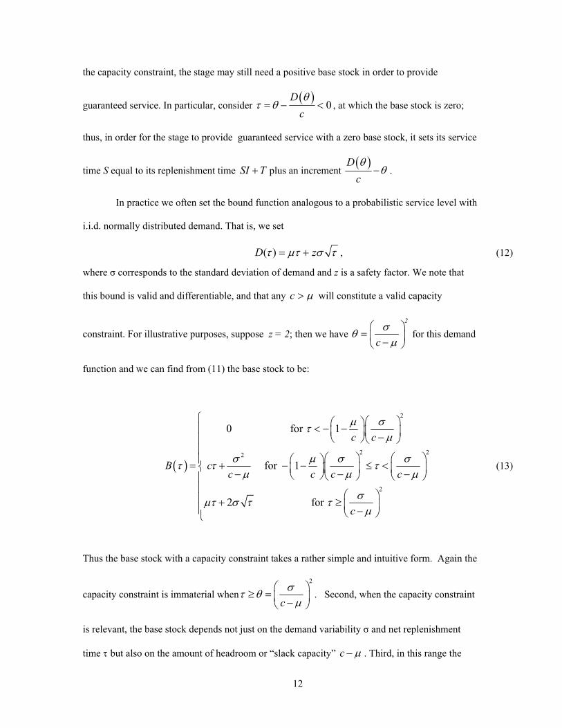
the capacity constraint, the stage may still need a positive base stock in order to provide
guaranteed service. In particular, consider ( ) 0
Dcθ
τ θ= − < , at which the base stock is zero;
thus, in order for the stage to provide guaranteed service with a zero base stock, it sets its service
time S equal to its replenishment time SI T+ plus an increment ( )Dcθ
θ− .
In practice we often set the bound function analogous to a probabilistic service level with
i.i.d. normally distributed demand. That is, we set
( )D zτ μτ σ τ= + , (12)
where σ corresponds to the standard deviation of demand and z is a safety factor. We note that
this bound is valid and differentiable, and that any c μ> will constitute a valid capacity
constraint. For illustrative purposes, suppose z = 2; then we have 2
cσθμ
⎛ ⎞= ⎜ ⎟−⎝ ⎠
for this demand
function and we can find from (11) the base stock to be:
Thus the base stock with a capacity constraint takes a rather simple and intuitive form. Again the
capacity constraint is immaterial when2
cστ θμ
⎛ ⎞≥ = ⎜ ⎟−⎝ ⎠
. Second, when the capacity constraint
is relevant, the base stock depends not just on the demand variability σ and net replenishment
time τ but also on the amount of headroom or “slack capacity” c μ− . Third, in this range the
13
base stock increases linearly at rate c in the net replenishment time. We plot the capacitated
base stock level (13) in Figure 2, together with the base stock level for the unconstrained case.
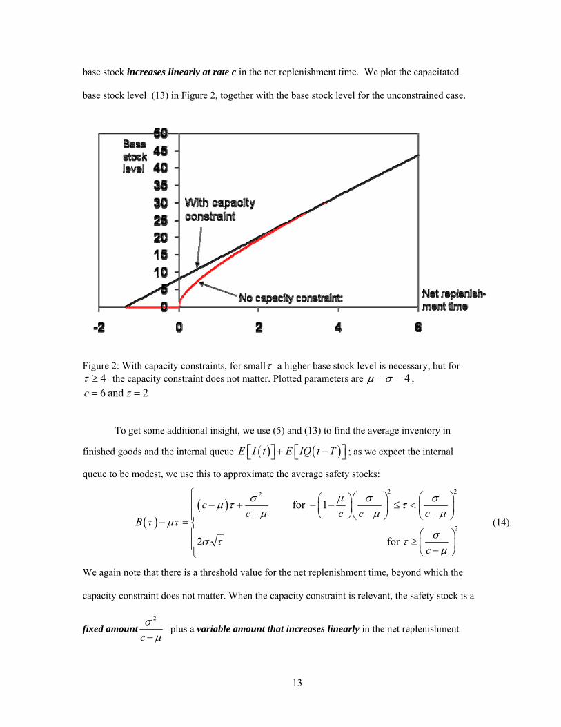
Figure 2: With capacity constraints, for smallτ a higher base stock level is necessary, but for 4τ ≥ the capacity constraint does not matter. Plotted parameters are 4μ σ= = , 6 and 2c z= =
To get some additional insight, we use (5) and (13) to find the average inventory in
finished goods and the internal queue ( ) ( )E I t E IQ t T⎡ ⎤ ⎡ ⎤+ −⎣ ⎦ ⎣ ⎦ ; as we expect the internal
queue to be modest, we use this to approximate the average safety stocks:
We again note that there is a threshold value for the net replenishment time, beyond which the
capacity constraint does not matter. When the capacity constraint is relevant, the safety stock is a
fixed amount2
cσμ−
plus a variable amount that increases linearly in the net replenishment
14
time. In contrast, for the uncapacitated system, the safety stock is proportional to the square root
of the net replenishment time. Finally, as the slack capacity goes to zero, the fixed amount of
safety stock increases hyperbolically; this is analogous to what happens to the waiting time in a
queue as utilization goes to one. Similar to the traditional square-root formula for safety stocks in
an uncapacitated setting, we regard (14) to be a valuable back-of-the-envelope heuristic in that it
succinctly displays how the safety stock depends on the slack capacity, the demand variability
and the net replenishment time.
3. Multiple stage model with base-stock ordering We now investigate a supply chain consisting of multiple stages, each of which may potentially
have a capacity constraint. In this network, each stage provides guaranteed service to its
customers (downstream neighbors), and operates according to a (local) base-stock policy. We
assume that customer demand is immediately propagated up through the system, so that in each
period t each node places an order on its suppliers equal to the sum of the customer demand from
all its adjacent downstream stages.
In order to describe the network and its characteristics, we index the nodes (or stages) and
denote the parameters kS , kT , kSI and kc specific to node k. We specify the topology of the
network by the directed edge set A where ( , )j k A∈ indicates that node j directly supplies (is
upstream of) node k. Customer facing nodes are defined by the set C, and have service times
exogenously specified; k kS s= for k C∈ . Other service times (and inbound service times) are
decision variables. The demand bound ( )kD is a bound on the demand from the customer
node(s) downstream of node k; see Graves and Willems (2000) for how to combine the bounds
from multiple demand streams. To facilitate the derivations to follow, we use operator notation
(see e.g. Griffel, 1985) to describe how we determine the base stock from the capacity constraint
15
and the demand bound. We use the symbol kψ to denote the continuous and node-specific
version of (10) as follows:
{ }0
( )( ) max ( )k k k knD D n c nψ τ τ
≥= + − (15)
As before, we set the base stock level to this quantity to ensure guaranteed service:
( ) ( )( )k k kB Dτ ψ τ= (16)
If node k does not have a capacity constraint, we can set kc = ∞ in (15) and find that
( ) ( )k kB Dτ τ= . At stage k, the total inventory that is on hand (either as finished inventory or
delayed in the internal queue) is ( ) ( )k kI t IQ t+ . We use the node-specific version of equation (5)
to characterize the average of this quantity, k kkI IQ+ :
( )( ) ( )k k k k k k k k kkI IQ D T SI S T SI Sψ μ+ = + − − + − (17)
We do not include inventory in process at stage k, because the average pipeline inventory is
proportional to the lead time kT and is not affected by the choice of service times. We assume that
stage k accrues holding costs proportional to k kI IQ+ , with the proportionality constant kh . This
is a simplification that we make for tractability. In many contexts one might expect the holding
cost for the internal queue inventory to be less than that for the finished good, as holding costs
should increase as we add more value to the product by processing. Nevertheless, we expect this
difference in holding costs to be modest; moreover, the average internal queue kIQ does not
depend on the service times and thus has no impact on the optimal solution.
We now formulate an optimization problem to find the service times that minimize the
total inventory holding cost, subject to providing guaranteed service at all nodes, for any demand
realization within the bounds.
16
( )
( )
, 1min ( )( ) ( )
, 0( , )
k k
N
k k k k k k k k kS SI k
k k
k j
k k
k kk k k k
k
h D SI T S SI T S
S SI kSI S j k A
S s k CD
SI T S kc
ψ μ
θθ
=
+ − − + −
≥ ∀≥ ∀ ∈
= ∈
+ − ≥ − ∀
∑
(18)
The decision variables are the service times, which are non-negative by the first constraint. The
second constraint assures that the inbound service time for each node is greater than or equal to
the maximum service time from its supply nodes. The third constraint fixes the service times for
customer-facing nodes to the exogenous specifications. The fourth constraint provides a lower
bound on the net replenishment time for each node, as discussed in the prior section, where θk is
specified by ( )'k k kD cθ = . Simpson (1958) and Graves and Willems (2000) formulate the
uncapacitated version of (18) for a serial system and for general networks, respectively. In both
cases, they observe that an optimal solution is on a corner of the solution space, since the problem
minimizes a concave objective function over a polyhedral set. We are therefore interested in
whether this observation applies here, namely whether the modified function ( )( )k kDψ τ is
concave for each node k. Under some reasonable technical conditions, this is in fact the case.
Proposition 1. Suppose ( )D τ is valid, and c valid with respect to ( )D τ . Then
{ }0
( )( ) max ( )n
D D n cnψ τ τ≥
= + − is concave on ( )[ , )
Dcθ
τ θ∈ − ∞ .
The proofs of all propositions are in the Appendix. Hence, the optimal solution will be at an
extreme point of the solution space. One practical implication of this is that an all-or-nothing
result holds for the capacitated serial system, analogous to the result proved by Simpson (1958)
for the uncapacitated case. Specifically, for a serial system either 0kS = , meaning that the stage
17
holds enough inventory to always provide immediate service, or alternatively,
( )kk k k k
k
DS SI T
cθ
θ= + − + in which case the base stock level 0kB = .
Simpson (1958) solved the uncapacitated version of (18) for a serial system by
enumeration. Graves and Willems (2000) develop an exact dynamic programming algorithm,
which can be used for networks with spanning-tree topology; Lesnaia (2004) shows how to
modify and implement this algorithm so that it is polynomial. We can modify the Graves-
Willems algorithm to solve (18) for spanning-tree networks with capacity constraints: we just
two changes. First, instead of using ( ) ( )k kB Dτ τ= for the base stock levels, we use the exact
characterization of the base stock necessary to handle capacity constraints given by (16). Second,
the lower bound on the net replenishment time is no longer zero, but is given by ( )k k
kk
Dcθ
θ − for
node k. To account for this, we just extend the search space for each iteration of the dynamic
program; this can be done with no change to the computational complexity.
4. Multiple stage model with censored order policy In the prior section we have shown how to generalize the GS framework and associated
optimization methods to encompass capacity constraints. In this section, we show that certain
improvements are possible, if the stages with capacity constraints modify their orders. The basic
idea with the censored policy is that a stage should not propagate a full order upstream, if it
knows that it will be unable to process such a quantity because of its capacity constraints.
Alternatively, we observe that there is no need for an internal queue at a capacitated stage; rather
the stage should place orders on its supplier so that these orders arrive at a rate consistent with the
stage’s capability to process the work.
18
To simplify the presentation, we consider a serial system, where we number the nodes
from downstream to upstream: node 1 is the customer facing node, and N is the most upstream
node. We will briefly discuss censorship in other network structures at the end of this section.
When we censor orders, each node can generate a different series of orders due to its
capacity constraint. We denote the order received by node k at time t by ( )kd t ; we denote its
bound by ( )kD t , where
( , ) ( ) , 0k kd t t D tτ τ τ+ ≤ ∀ ≥ . (19)
Accordingly, we write 1( ) ( )d t d t= and 1( ) ( )D t D t= for customer demand and its bound.
We assume that each node k never orders more than its capacity kc . Thus whenever its demand
exceeds its capacity ( )( )k kd t c> , it orders less than the demand and creates a shortfall. When
demand falls below kc again, stage k increases its order to reduce the shortfall. To this end, node
k keeps a backlog ( )kBL t of this shortfall, equal to the amount of its demand for which it has yet
to place a replenishment order. Node k will increase its order whenever it has a backlog and
capacity is available. We now specify the orders placed at time t by node k on node k + 1 by:
1( ) min( ( ) ( 1), )k k k kd t d t BL t c+ = + − . (20)
We can specify the backlog ( )kBL t recursively:
{ }{ }{ }
{ }
( ) max ( 1) ( ) ,0
max max (( 2) ( 1) ,0 ( ) ,0
max ( , ) .
k k k k
k k k k k
k kn Z
BL t BL t d t c
BL t d t c d t c
d t n t c n∈
= − + −
= − + − − + −
= − −
(21)
Here we assume that the system starts at t = 0 with ( ) ( )0, 0k kBL t d t= = for all 0t ≤ . In each
period, stage k adds the difference between its demand and capacity, ( )k kd t c− , to the backlog,
subject to keeping the backlog non-negative.
19
We can show that the inventory for node k, ( )kI t , is the inventory for the uncapacitated
problem, net of the backlog at time k kt SI T− − . Since the replenishment time is k kSI T+ ,
anything in the backlog at node k at time k kt SI T− − cannot be available by time t to meet
demand at node k. Thus, we have:
{ }{ }
( ) ( , ) ( )( , ) max ( , )
max ( , )
k k k k k k k k k
k k k k k k k k k k kn Z
k k k k k kn Z
I t B d t SI T t S BL t SI TB d t SI T t S d t n SI T t SI T c n
B d t n SI T t S c n∈
∈
= − − − − − − −
= − − − − − − − − − − −
= − − − − − −
(22)
Except for the fact that the demand kd is now stage-specific, this is equivalent to the inventory
equation for a capacitated stage that does not censor its orders, namely equivalent to (5). That is,
when considering the inventory ( )kI t at some stage, it makes no difference whether items are
waiting in the internal queue, or whether the orders placed by that stage were temporarily put into
a backlog because of censorship. In both cases the quantities that start and finish their processing
in each period are the same. Thus if node k has a capacity constraint, we can use equation (16) to
determine the base stock level that guarantees service, regardless of whether a censored order
policy is employed or not. Thus we set the base stock level by
( ) ( )( )k k kB Dτ ψ τ= .
where we use the operator kψ defined in (15).
There are a couple of immediate implications from the censored order policy. First, in
comparison to the base-stock order policy the average inventory will be less (for a fixed base-
stock level), because orders never exceed capacity and there is no internal queue. We obtain the
total average inventory by taking the average of (22):
( ) kk k k k kI B SI T S BLμ= − + − − (23)
Thus in the case of censored orders, we need to calculate the term kBL , in order to determine
average inventory levels and costs. The term kBL depends on specific properties of the demand
20
distribution, and is generally difficult to estimate; we discuss this topic in greater detail in the
Appendix. However, we note that kBL does not depend on the service times. Thus we do not
need to determine kBL to find the optimal safety stocks; rather, the sole purpose for determining
kBL is for the determination of the average inventory level given by (23)
A second implication of the censored order policy is that the censored order is bounded
by the capacity at stage k, i.e., ( )1( )k kd t c+ ≤ ; thus, a looser capacity constraint at stage k + 1
( )1k kc c+ > is irrelevant. Indeed, any upstream capacity constraint that is greater than a
downstream capacity limit can be ignored.
A third more significant implication of the censorship is that the upstream stages will face
a different demand bound, one that is censored by node k’s capacity. We describe next how to
determine the bound on the censored orders.
Proposition 2. Suppose 1( ) min( ( ) ( 1), )k k k kd t d t BL t c+ = + − where kBL is given by (21), and
initialized with ( ) 0kBL t = for 0t ≤ . Assume that kD is a valid bound for kd (that is,
( , ) ( ) , 0k kd t t D tτ τ τ+ ≤ ∀ ≥ ), and that kc is valid with respect to ( )kD τ . Then
1 1( , ) ( ) ( )( ) , 0k k k kd t t D D tτ τ τ τ+ ++ ≤ = Φ ∀ ≥ (24)
where kΦ is defined by
( )( ) min( , ( ))k kD c Dτ τ τΦ = . (25)
This bound is tight, in that for every 0τ ≥ there is some ( , ) ( )k kd t t Dτ τ+ = .
Thus we have an evaluative model for a serial system with capacity constraints and censored
orders. We assume that the demand is propagated up the supply chain by (21), with (22) to
account for the backlog of orders. We can then use Proposition 2 to compute the demand bound
at each node. Given these demand bounds we can then use (16) to characterize the necessary
base stock level for each node. Given the base stock level, we can calculate the average
21
inventory from (23). We summarize these iterative steps in Table 1, with a comparison to the
uncapacitated model.
No capacity constraint at node k Capacity constraint kc at node k
Orders placed 1( ) ( )k kd t d t+ = 1( ) min( ( ) ( 1), )k k k kd t d t BL t c+ = + −
Bound on orders placed
1( ) ( )k kD Dτ τ+ = 1( ) ( )( )min( , ( ))k k k
k k
D Dc D
τ ττ τ
+ = Φ=
Base stock level ( ) ( )k k k kB Dτ τ=
{ }0
( ) ( )( )max ( )
k k k k k
k k kn
B DD n c n
τ ψ τ
τ≥
=
= + −
Average inventory
( )k k k kI B τ μτ= − ( ) ( ) kk k k kI t B BLτ μτ= − −
Table 1: Summary of node properties in serial system supply chain with capacity constraint(s) and censored base stock policy; we use kτ to denote the net replenishment time at node k.
We can now embed this model in an optimization, analogous to (18), to find the best choices for
the service times. In the following proposition we establish that the demand bounds and capacity
constraints are valid as defined earlier; as these properties were necessary to derive the necessary
base stock levels. We also show that the resulting base stock levels ( )k kB τ are concave functions.
Proposition 3. Suppose that end demand 1( ) ( )d t d t= is bounded by ( )D τ and that ( )D τ is
valid. Assume further that some subset of nodes has capacity constraints, and that these are all
valid with respect to ( )D τ , and that these kc are decreasing with increasing k. Finally, suppose
that each node k places orders 1( )kd t+ according to (20). Then
a) All orders kd are bounded by ( )kD τ , as specified by (24)
b) All ( )kD τ are valid
c) lc for nodes with capacity constraints are valid with respect to ( )kD τ , for all l k≥
d) The base stock levels ( )kB τ as specified by (16) ensure that ( ) 0kI t ≥
22
e) All ( )kB τ are concave in τ .
Thus we have shown that in a serial-system supply chain with capacity constraints and
censorship, we can compute the demand bounds and necessary base stock levels by recursively
applying a sequence of functional operators, as summarized in Table 1. Thus, as for the case of
base-stock ordering, we can use the algorithm developed by Graves and Willems to find the
optimal service times for a serial-system supply chain with both capacity constraints and
censorship, after only small modifications.
We can extend the results in this section to arborescent (assembly tree) supply chain
topologies in which each node has a single customer node. The iterative steps laid out in Table 1
apply directly, but with one modest modification: the order placed by node k (given by (21)) is
now placed concurrently on each of the suppliers to node k. Again we can use the existing
algorithm from Graves and Willems to find the optimal service times and safety stocks.
The extension to supply chains with several end demand nodes (as in a distribution network,
for example) is not as immediate. The primary challenge is to determine how to combine multiple
demand bounds, each of which may be censored. For uncapacitated supply chains, Graves and
Willems (2000) propose how to set bounds if demand streams are independent, and the bound is
set analogous to a probabilistic service level, as in (12). They also propose bounds for larger or
smaller measures of risk pooling. If one or more bound are generated by a censored order policy,
then it is not clear how best to merge bounds from multiple streams. Of course, one can always
obtain a valid and conservative bound by simply adding the bounds of downstream stages; we
leave for future research the question of how to improve upon this demand bound for supply
chains operating with a censored order policy.
5. Numerical experiments To examine the impact of capacity constraints, we perform a set of numerical
experiments. We consider a serial system with N = 5 stages or nodes, and with a demand bound
23
given by ( )D zτ μτ σ τ= + , with the parameters ( , , ) (40, 2, 20)zμ σ = . We have three
alternatives each for the holding costs and for the lead-times, as shown in Table 2.
Holding costs ( )5 4 3 2 1, , , ,h h h h h Lead-times ( )5 4 3 2 1, , , ,T T T T T
Table 2: Alternative structures for supply chain lead-time and cost accumulation
In all cases the total lead time is 100 and the holding cost at the customer-facing stage 1 is 1.00.
The term “upstream-heavy” means that the upstream stages have the longest lead-times or have
the largest echelon holding costs.4 Similarly, downstream-heavy means that the largest lead-
times or echelon holding costs are at the downstream stages.
We assume each supply chain has a single capacity constraint. We allow the constraint to
be at any of the five stages, and we set the capacity to be one of five values from the set (42, 45,
50, 60, 70), representing 0.1μ σ+ up to 1.5μ σ+ . Thus, we specify 3 3 5 5 225× × × = test
problems: three choices for holding costs, three choices for lead-times, five locations for the
capacity constraint, and five values for the capacity.
For each test problem, we solve for both the base-stock policy and the censored ordering
policy. To benchmark the performance of the uncapacitated GS model, we also solve the
corresponding uncapacitated problem to find its inventory holding cost and optimal policy. The
uncapacitated solution is typically not feasible for the capacitated problem in that it will not
provide guaranteed service. However, we can adapt the uncapacitated solution to create a feasible
censored ordering policy for the capacitated problem; we assume the decoupling safety stocks are
located as given by the uncapacitated solution, and then find the censured ordering policy that
4 The echelon holding cost for stage k is 1k kh h +− .
24
provides guaranteed service for these safety stock locations. In this way we can evaluate the
performance of the uncapacitated solution in the presence of a capacity constraint.
In Table 3 we report the results for the test problems with capacity c = 45, which are
indicative of the behavior at the other capacity levels. For each of the 45 test problems we report
the costs of the censored policy, the base-stock policy, and the adapted uncapacitated policy; in
each case these costs are given as a percentage of the cost for the corresponding uncapacitated
problem, which is also given in the table. We make three observations.
Location of Capacity Constraint
Holding cost profile
Lead time profile
Uncap Cost
5 4 3 2 1
Upstream Heavy
400 99% 102% 105%
104% 111% 107%
106% 116% 109%
103% 114% 111%
89% 100% 93%
Constant 400 103% 106% 105%
106% 112% 107%
108% 116% 109%
109% 118% 111%
91% 100% 93%
Upstream Heavy
Downstream Heavy
400 104% 107% 105%
107% 112% 107%
109% 116% 109%
110% 118% 111%
92% 100% 93%
Upstream Heavy
368 98% 100% 98%
95% 100% 97%
93% 102% 105%
87% 102% 107%
73% 100% 89%
Constant 394 98% 100% 98%
99% 104% 101%
101% 112% 103%
103% 115% 105%
86% 100% 88%
Constant
Downstream Heavy
400 101% 103% 103%
104% 108% 105%
106% 111% 107%
108% 115% 109%
91% 100% 93%
Upstream Heavy
268 100% 100% 100%
97% 100% 97%
91% 100% 91%
81% 100% 97%
65% 100% 73%
Constant 346 100% 100% 100%
98% 100% 98%
95% 102% 101%
96% 109% 104%
78% 100% 87%
Downstream Heavy
Downstream Heavy
392 100% 100% 100%
98% 100% 98%
98% 103% 101%
101% 113% 104%
86% 100% 89%
25
Table 3: Results for test problems with capacity constraint 45c = . In each cell, the three numbers are the normalized costs for the censored order policy (top), the base-stock policy (middle) and the adapted uncapacitated policy (bottom). The normalized costs are given as a percentage of the corresponding unconstrained problem, whose cost is in the third column.
First, as expected, the censored ordering policy dominates the base-stock policy. Indeed,
for the 225 test problems, we found an average cost reduction of 8.0% when we replace the base-
stock policy with the censored ordering policy. Thus when capacity constraints are present, a
strong case can be made for censoring the orders at that stage.
Second, the adapted uncapacitated policy performs quite well as a heuristic. For 75% of
the test problems with capacity c = 45, the cost for the adapted policy is within 3% of that for the
censored ordering policy. However, when the upstream lead-times are long and the constraint is
downstream at stage 1 or 2, the adapted uncapacitated policy can cost 8 to 20% more than the
censored ordering policy.
The third observation is that the cost impact of the capacity constraint is not great. For
the test problems with capacity c = 45, the incremental cost relative to the cost for the
uncapacitated supply chain is at most 10%, and is less than 5% for 80% of the cases. More
surprising, though, is the fact that under censorship the costs are often less than in the
corresponding problem without capacity constraints. Indeed, for the 225 test problems, we find
that the total cost for the constrained system with a censored ordering policy is on average 3.6%
lower than the total cost for the corresponding unconstrained base-stock system.
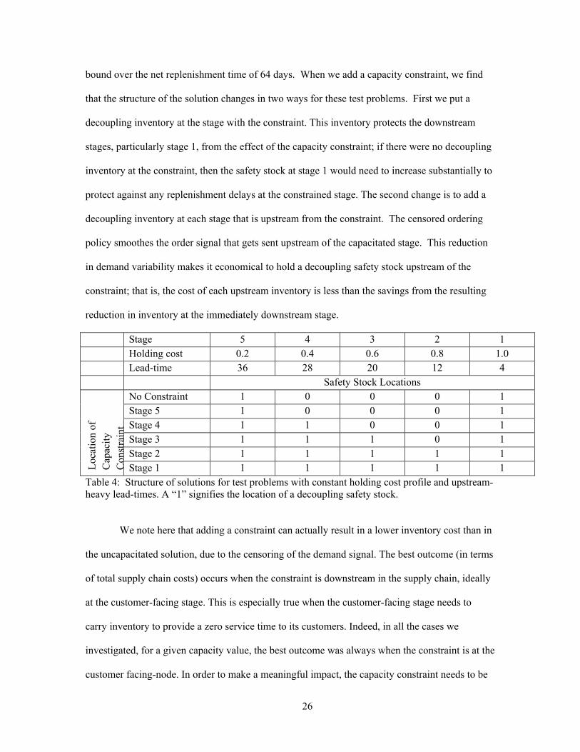
To get a better understanding of the last two observations, we consider the test problems
with a constant holding cost profile and upstream-heavy lead-times. In Table 4, we show the
locations of the decoupling safety stocks for the uncapacitated solution and for the censored
ordering policy for each location of the constraint. In the unconstrained problem, the optimal
solution is to have one large inventory (and a long net replenishment time) at the first, customer-
facing stage and a small inventory at stage 5; the inventory at stage 1 is sized to cover the demand
26
bound over the net replenishment time of 64 days. When we add a capacity constraint, we find
that the structure of the solution changes in two ways for these test problems. First we put a
decoupling inventory at the stage with the constraint. This inventory protects the downstream
stages, particularly stage 1, from the effect of the capacity constraint; if there were no decoupling
inventory at the constraint, then the safety stock at stage 1 would need to increase substantially to
protect against any replenishment delays at the constrained stage. The second change is to add a
decoupling inventory at each stage that is upstream from the constraint. The censored ordering
policy smoothes the order signal that gets sent upstream of the capacitated stage. This reduction
in demand variability makes it economical to hold a decoupling safety stock upstream of the
constraint; that is, the cost of each upstream inventory is less than the savings from the resulting
reduction in inventory at the immediately downstream stage.
Stage 1 1 1 1 1 1 Table 4: Structure of solutions for test problems with constant holding cost profile and upstream-heavy lead-times. A “1” signifies the location of a decoupling safety stock.
We note here that adding a constraint can actually result in a lower inventory cost than in
the uncapacitated solution, due to the censoring of the demand signal. The best outcome (in terms
of total supply chain costs) occurs when the constraint is downstream in the supply chain, ideally
at the customer-facing stage. This is especially true when the customer-facing stage needs to
carry inventory to provide a zero service time to its customers. Indeed, in all the cases we
investigated, for a given capacity value, the best outcome was always when the constraint is at the
customer facing-node. In order to make a meaningful impact, the capacity constraint needs to be
27
only slightly higher than average demand; in fact, for all the examples with censorship at the
customer-facing stage, the lowest tested capacity 0.1 42μ σ+ = always gave the best value.
However, we also know from (13) that as the capacity approaches average demand, the necessary
base stock level goes to infinity.
When determining the average cost for the censored ordering policy, one must calculate
the term kBL in (23). We discuss this topic in greater detail in the Appendix. We note here that
this term will depend on specific properties of the demand process, properties which up until this
point have not been specified. In the experiments listed here we estimated this term using both the
formula (A28) and the numerical estimates of kBL based on assuming that demand is normally
distributed and i.i.d. The average difference in terms of total costs was only 2.1%, and none of
the overall results and conclusions were different from those presented here. We also emphasize
that while the value of the term kBL does impact the total cost, it does not affect the optimal
solution, nor does a poorly estimated kBL compromise the guaranteed service constraint.
6. Conclusions and discussion We have analyzed the inclusion of capacity constraints in the context of the GS model for safety
stocks in multi-echelon supply chains. We have shown how to extend the single-stage base-stock
model to include a capacity constraint. We have used this result to model multi-stage supply
chains with capacity constraints. We have characterized the base stock level for two cases that
depend on how orders are propagated across the supply chain. In both cases we can extend the
structural findings and solution methods that have been developed for the uncapacitated supply
chains, e.g., by Simpson (1958) and Graves and Willems (2000).
In general we expect to need more safety stock when we have capacity constraints.
Indeed, as is clear from (13), the costs associated with capacity constraints can be arbitrarily
28
large, as the slack capacity goes to zero. However, for stages with sufficiently long net
replenishment time, there may be no additional cost associated with capacity constraints.
When we use the censored order policy, the costs are not only lower than in the
corresponding capacity-constrained problem with base-stock ordering, but frequently even lower
than in the unconstrained problem as well. Intuitively, a capacity constraint typically increases the
base stock level for the stage with the constraint (Equation (10); Figure 2); however, the resulting
increase in the average inventory may not be as great because some of the increase in the base
stock ends up as the positive backlog. Furthermore, the censored orders can be much smoother
than the original demand process. As a consequence there can be a substantial reduction in the
need for inventory at upstream nodes (Proposition 2; Table 4). The total effect may imply higher
or lower costs depending on the specific parameters.
On a more abstract level, it may seem surprising or even paradoxical that adding a
constraint can lead to a better solution. The explanation is that we have in effect expanded the
space of possible ordering policies. The original GS model from Simpson (1958) is based under
the assumption that all stages operate with a base stock policy. The results from our experiments
illustrate that this policy need not be optimal in a multi-echelon supply chain with guaranteed
service. Indeed, one might want to introduce a censored order policy even in the absence of
capacity constraints in order to get these benefits. In our experiments the best outcome was when
the customer-facing node was tightly constrained. This suggest that it may be preferable for the
first stage in a supply chain to act as a damper, whereby it absorbs the variability from a demand
signal, rather than pass along this variability to the rest of the supply chain.
As we have noted, the costs (but not the optimal solution) of systems with censorship
depend on the term kBL , which in turn depends on specific properties of the demand
distribution, and which moreover appears difficult to estimate. This suggests opportunities for
future research, but also hints at certain fundamental limitations on the ability to predict the
29
performance of censored systems. It is a rare practical situation in which one can be confident
about higher-order properties of the demand distributions (although, in our experiments, the total
system costs were quite similar when we estimated kBL in different ways). The challenges of
calculating kBL also make it difficult to find “optimal” censorship value(s) and location(s),
although surely improvements are possible over the simple brute-force searches we presented in
our experiments.
Another opportunity for future research is to examine how to extend the methods for
uncapacitated supply chains modeled as general networks (Humair and Willems, 2006, 2008) to
account for capacity constraints.
A final line of research might relax the assumption that the customer service times are
exogenously set. One might include within the safety stock optimization the decision on the
customer service time, where there is a penalty cost associated with a longer customer service
time. Alternatively a firm might segment its customers into different classes, each with a
customer service time and a price; the research question might be how to set the segments in
conjunction with the supply-chain safety stock optimization.
Acknowledgements
This research has been funded in part by the Singapore MIT Alliance (SMA) and by Dr. Marcus
Wallenberg’s Foundation for Education in International Industrial Management. The authors
thank the reviewers for their helpful comments on an earlier version of this paper.
30
Appendix 1: The average backlog
Here we consider estimating kBL .We recall that this quantity is necessary to understand the
expected inventory costs for a node with capacity constraints and censorship. However, kBL
does not depend on the decision variables (the service times) and it is not needed in order to
obtain or implement the optimal solution.
We note that the back log described in (21) behaves rather like a queue - there is a random
quantity of arrivals every period, and a fixed, maximum processing rate. Even though kBL
operates in discrete time, we can use continuous-time queuing theory as an approximation.
Suppose that we model the internal queue with an M/D/1 queue with arrival rateλ , and
deterministic processing time s. We then seek λ and s that agree with the average μ and
standard deviation σ of demand per period, or cμ
and cσ
if we normalize with respect to
capacity. That is, we model demand using a continuous-time model with Poisson arrivals, but we
ensure that the probability distribution of the number of arrivals agrees in first and second
moments to our original process. We are making a second order, continuous-time, approximation:
s
c
sc
μ λ
σ λ
=
= (A26)
Conversely, if we already have a mean and standard deviation for demand, we can invert the
relations (A26) solve for s andλ .
31
2
22
2
2
2
2
ssc
s
s
sc c
μ μ μλ σσ
σμμ μλ
σ
= = =⎛ ⎞⎜ ⎟⎝ ⎠
=
= =
(A27)
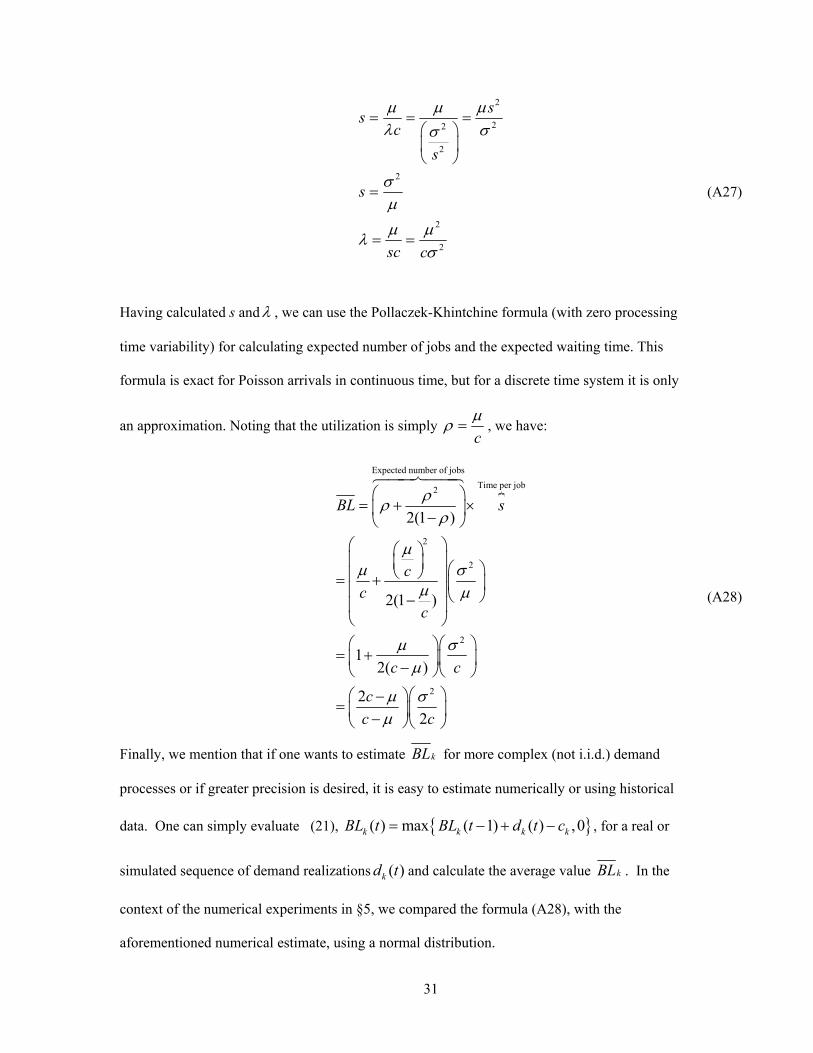
Having calculated s andλ , we can use the Pollaczek-Khintchine formula (with zero processing
time variability) for calculating expected number of jobs and the expected waiting time. This
formula is exact for Poisson arrivals in continuous time, but for a discrete time system it is only
an approximation. Noting that the utilization is simply cμρ = , we have:
Expected number of jobsTime per job2
2
2
2
2
2(1 )
2(1 )
12( )
22
BL s
cc
c
c c
cc c
ρρρ
μμ σ
μ μ
μ σμ
μ σμ
⎛ ⎞= + ×⎜ ⎟−⎝ ⎠
⎛ ⎞⎛ ⎞⎜ ⎟⎜ ⎟ ⎛ ⎞⎝ ⎠⎜ ⎟= + ⎜ ⎟⎜ ⎟⎝ ⎠−⎜ ⎟⎝ ⎠
⎛ ⎞⎛ ⎞= + ⎜ ⎟⎜ ⎟−⎝ ⎠⎝ ⎠
⎛ ⎞⎛ ⎞−= ⎜ ⎟⎜ ⎟−⎝ ⎠⎝ ⎠
(A28)
Finally, we mention that if one wants to estimate kBL for more complex (not i.i.d.) demand
processes or if greater precision is desired, it is easy to estimate numerically or using historical
data. One can simply evaluate (21), { }( ) max ( 1) ( ) ,0k k k kBL t BL t d t c= − + − , for a real or
simulated sequence of demand realizations ( )kd t and calculate the average value kBL . In the
context of the numerical experiments in §5, we compared the formula (A28), with the
aforementioned numerical estimate, using a normal distribution.
32
c 42 45 50 60 70
Simulated/ Normal 88.5 29.6 10.6 2.5 0.7
PK-formula/ Poisson 104.8 44.4 24.0 13.3 9.5
Table 5: kBL for 40, 20μ σ= = , and various censorship values c.
The continuous-time formula appears to give much higher values of kBL for large capacities, but
for smaller capacities the results are reasonably similar. An explanation for this is the continuous
time assumption in the Pollaczek-Khintchine formula; there will frequently (and on average) be a
queue just after each job arrival, but in the discrete-time system processing effectively happens
“after” all the job arrivals in each period. This effect becomes less and less significant as the
capacity constraint becomes smaller and smaller and the busy periods become longer and longer.
While these methods yield rather different results, the term kBL is typically only
responsible for a small portion of all costs. Fortunately, the different methods are increasingly
similar as the cost contribution from the kBL term grows and makes a significant contribution.
Thus in the experiments we performed, the average total cost difference between the two methods
was, on average, only 2.1%.
33
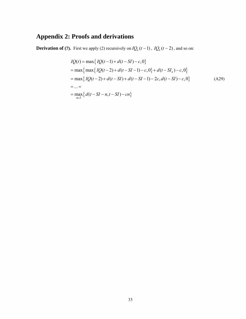
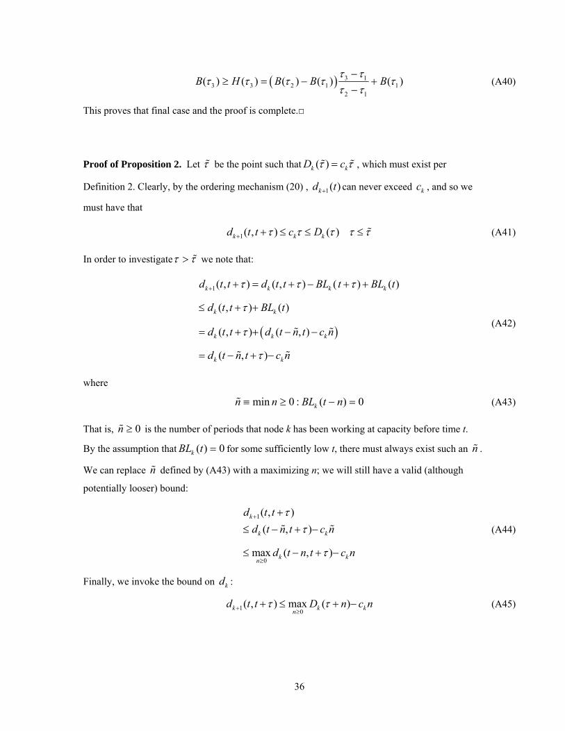
Appendix 2: Proofs and derivations
Derivation of (7). First we apply (2) recursively on ( 1)kIQ t − , ( 2)kIQ t − , and so on:
{ }{ }{ }
{ }
{ }
( ) max ( 1) ( ) ,0
max max ( 2) ( 1) ,0 ( ) ,0
max ( 2) ( ) ( 1) 2 , ( ) ,0...max ( , )
k
n Z
IQ t IQ t d t SI c
IQ t d t SI c d t SI c
IQ t d t SI d t SI c d t SI c
d t SI n t SI cn∈
= − + − −
= − + − − − + − −
= − + − + − − − − −
= =
= − − − −
(A29)
34
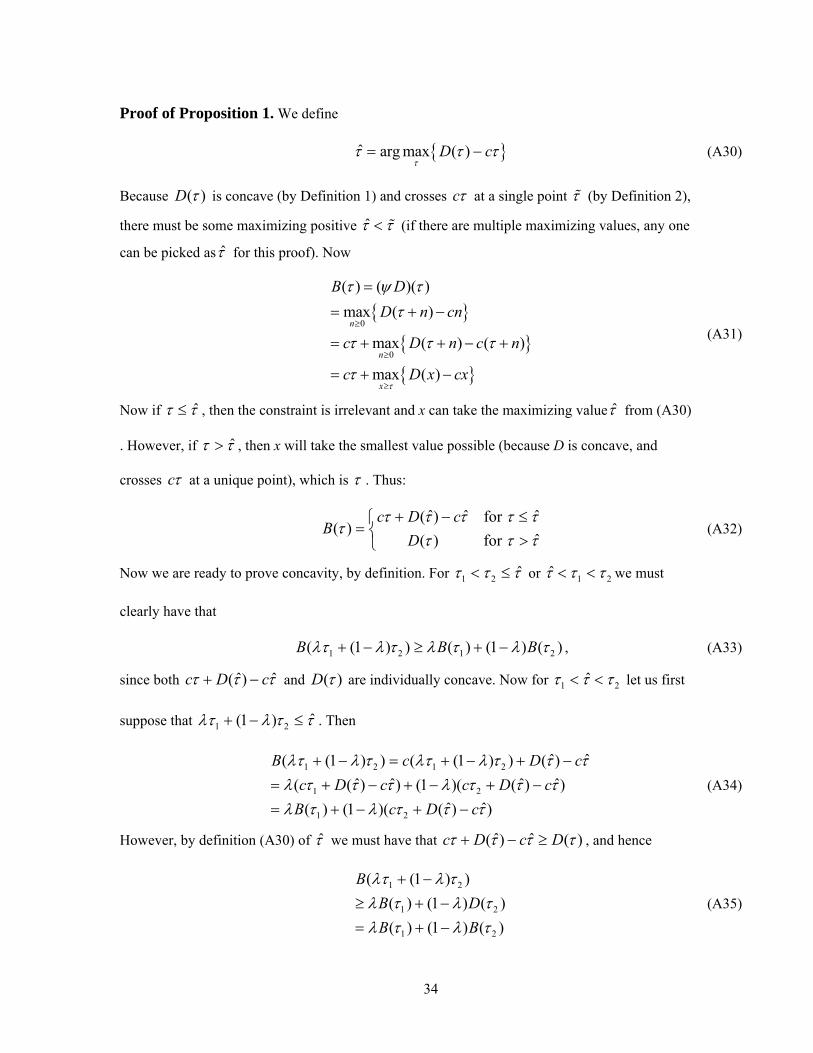
Proof of Proposition 1. We define
{ }ˆ arg max ( )D cτ
τ τ τ= − (A30)
Because ( )D τ is concave (by Definition 1) and crosses cτ at a single point τ (by Definition 2),
there must be some maximizing positive τ̂ τ< (if there are multiple maximizing values, any one
can be picked asτ̂ for this proof). Now
{ }
{ }{ }
0
0
( ) ( )( )max ( )
max ( ) ( )
max ( )
n
n
x
B DD n cn
c D n c n
c D x cxτ
τ ψ ττ
τ τ τ
τ
≥
≥
≥
=
= + −
= + + − +
= + −
(A31)
Now if ˆτ τ≤ , then the constraint is irrelevant and x can take the maximizing valueτ̂ from (A30)
. However, if ˆτ τ> , then x will take the smallest value possible (because D is concave, and
crosses cτ at a unique point), which is τ . Thus:
ˆ ˆ ˆ( ) for
( )ˆ( ) for
c D cB
Dτ τ τ τ τ
ττ τ τ
+ − ≤⎧= ⎨ >⎩
(A32)
Now we are ready to prove concavity, by definition. For 1 2 ˆτ τ τ< ≤ or 1 2τ̂ τ τ< < we must