Strategic vertical integration without foreclosure

E. Avenel ∗, Université de Toulouse (GREMAQ) & UPMF-Grenoble 2

January 8, 2003

Abstract : We determine the endogenous degree of vertical integration in a model

of successive oligopoly that captures both efficiency gains and strategic effects. We show

that vertical merger waves can be expected to stop by themselves before integration is

complete. Consequently, vertical foreclosure plays no significant role in this paper that

claims for a soft approach of vertical integration by antitrust authorities.

JEL Classification numbers : L22, L40.

Key Words : Merger waves, vertical integration, vertical foreclosure.

1 Introduction

It is well known that there are three main motivations to vertically integrate for an

upstream firm and a downstream firm. The first motivation documented in the economic

literature is the minimization of transaction costs by the choice of an optimal governance

structure for contractual relationships. In this strand of literature, vertical integration is

viewed as one possible governance structure. The second motivation is described by the

property rights literature that argues that the optimal allocation of property rights on

assets allows firms to reduce to the minimum the problem of the ex ante nonoptimality of

investment levels. Vertical integration is just one possible allocation of property rights and,

in fact, one has to distinguish between different types of vertical integration, depending

∗GREMAQ, Université des Sciences Sociales, Manufacture des Tabacs, 21 allée de Brienne, 31000

Toulouse, France. E-mail : eric.avenel@upmf-grenoble.fr

1

on who owns the assets (the downstream or the upstream firm). There are substantial

differences between these two ways to envision vertical integration (see Whinston (2001)

for more details), but both claim that vertical integration may allow firms to achieve

efficiency gains that nonintegrated firms could not achieve. The third motivation for

vertical integration is quite different. It relies on the analysis of vertical integration in a

strategic context and claims that vertical integration may be profitable because it allows

firms to reduce their costs through the elimination of double marginalization (this is in

fact a story about efficiency gains resulting from vertical integration) and thus to be in

a better position when competing with their rivals on the final market. At this point,

the story goes on with the ”vertical foreclosure” argument. Indeed, it is claimed that

vertical integration is also a rising rivals’ costs strategy because the integrated firm leaves

the intermediate market, nonintegrated upstream firms enjoy more market power and rise

the intermediate price that they charge to independent downstream firms. So, according

to this foreclosure story, vertical integration is profitable both because it reduces the

double margin for the merging firms and because it increases the double margin for those

who remain independent. There is a quite hot debate on foreclosure since the Chicago

school economists criticized the first, unformal version of the foreclosure theory. The

seminal paper by Ordover, Saloner and Salop (1990) layed the foundations for a new

foreclosure theory based on more convincing game theoretic arguments. More recently,

Avenel (2000), Choi and Yi (2000) and Church and Gandal (2000), relying on the idea that

firms can make strategic technological choices that commit them to foreclose their rivals,

have proved that vertical foreclosure can emerge in models in which vertical integration

is endogenous, technological choices are endogenous and there is no assumption on the

ability of integrated firms to commit to a price.

Although the debate on vertical foreclosure is extremely interesting, it is quite unfortu-

nate that the analysis of vertical integration in a strategic context has focused exclusively

on this issue. Indeed, the previously quoted models assume that the upstream indus-

try is a duopoly, so that under partial vertical integration, the independent upstream

firm enjoys monopoly power on the residual demand and the rising rivals’ costs is quite

strong. But what about industries with less concentrated upstream markets ? Clearly, if

2

competition is quite strong between upstream firms, the vertical merger of one upstream

firm with a downstream firm will not allow its upstream competitors to substantially rise

their price and the rising rivals’ costs effect will be very small. It is in fact absent as

soon as there are three (identical) upstream firms, constant returns to scale and Bertrand

competition. This is precisely the framework that we use in this paper. This prediction

that vertical foreclosure is not an issue as long as there is a substantial degree of com-

petition on the residual intermediate market may well explain why it is so difficult to

find empirical evidence of foreclosure (Rosengren and Meehan (1994), for example, find

no empirical support for the foreclosure theory). Indeed, duopoly competition is not the

general rule on intermediate markets. We think that it is time to develop a theory of

endogenous vertical integration in strategic contexts that (i) takes into account the effi-

ciency gains resulting from vertical integration as described in the transaction costs and

property rights literatures and (ii) takes into account the possibility of vertical foreclosure

without putting an exagerate emphasis on it. The model that we describe below is an

attempt to contribute to such a theory of vertical integration.

This model is closely related to McLaren (2000), since we also determine the degree of

vertical integration resulting from simultaneous integration choices in a industry composed

of the same number of upstream and downstream firms. There is however a difference

between the two models that happens to be critical. In McLaren (2000), there is no

competition between downstream firms on the final market or, equivalently, the efficiency

gains associated to vertical integration take the form of lower fixed costs for downstream

firms. They thus have no impact on prices and outputs on the final market. In my

model, the efficiency gains take the form of lower marginal costs for upstream firms, this

reduction leading to lower marginal costs for downstream firms. Prices and outputs then

depend on the vertical structure of the industry. This effect is strong enough to reverse the

main result of McLaren (2000). There is no longer strategic complementarity in vertical

integration, but rather strategic substituability, with profoundly different implications in

terms of how antitrust policy should deal with vertical integration.

The structure of the article is as follows. In the next section, we present the model and

determine equilibrium prices and outputs in the various possible industrial structures. In

3

section 3, we examine how the technological choice of firms is related to their decision

regarding vertical integration. In section 4, we establish our main result on the structural

and technological features of the industry in equilibrium. Section 5 is devoted to the

analysis of the implications for antitrust policy. In section 6, we discuss welfare. Section

7 concludes.

2 The model

In this section, we describe the model, beginning with the technologies available to firms.

2.1 Technologies

We assume that there exists a generic technology that any firm in the industry (upstream,

downstream or integrated) can adopt. Furthermore, all the firms using this technology

are equally efficient, with constant marginal costs of production taken equal to c > 0 for

upstream firms and normalized to 0 for downstream firms. Alternatively, each pair of

firms (either an integrated firm or a pair of independent upstream and downstream firms)

can adopt a specific technology that is only available to this pair of firms and that is more

efficient than the generic technology. More precisely, the upstream marginal cost is equal

to c−ε > 0 and the downstream cost is equal to 0. The specificity of the technology impliesthat a specific intermediate good is less efficient when used with another technology. We

denote by δ the cost, assumed to be constant, of adapting one unit of specific input to

the generic technology or another specific technology. This is also the cost of adapting a

unit of generic intermediate good to a specific technology. It may be convenient to think

of the adoption of a specific technology as the decision to build two new production units

located at the same place, wide away from other production units. Transportation costs

are reduced between the two plants (this is ε), but increased between each of the two

plants and any plant located elsewhere (this is δ). We assume that the adoption of a

specific technology requires investment in specific assets both upstream and downstream.

As a consequence, a pair of independent firms can adopt the specific technology available

to it only if both firms agree on this decision. Given the incomplete nature of contracts

4

in this model, vertical integration may be profitable to a pair of firms because it allows

them to adopt the more efficient, specific technology. Given these premisses, we now can

describe the model.

2.2 Set-up

We consider an industry composed of n ≥ 2 downstream firms (Di)i=1,...,n and the same

number n of upstream firms (Ui)i=1,...,n that supply them with an intermediate good that

they transform into a final good on a one for one basis. We assume that final goods are

horizontally differentiated and, more specifically, that the demand for good i is given by

qi = α− βpi + γXj 6=ipj (1)

In (1), pi is the price charged by Di, pj the price charged by Dj and qi the quantity

sold by Di for the vector of prices. We denote by P the vector of prices on the final

market.

For this demand function to make sense, we must assume that condition (2) below

holds. If it would not, a general increase in prices would increase the output of each firm

and the total output.

γ < β/ (n− 1) (2)

As regards competition on the intermediate market, we assume that upstream firms

are engaged in price competition and denote by W = (wi)i=1,...,n the vector of prices

charged by upstream firms. We further assume that the upstream firms using the generic

technology produce an homogeneous intermediate good, whereas each usptream firm using

a specific technology produces an intermediate good different from every other variety of

the intermediate good. It is possible to transform intermediate goods to adapt them to a

technology they were not designed for at a cost δ. We assume, without loss of generality,

that this cost is supported by upstream firms.

5

The model is built on a three stage game. In the first stage, each pair Ui −Di has todecide on two points, integration and technology. At the end of stage 1, there are thus

four types of pairs of firms. We denote by nSG the number of pairs of firms that are not

integrated (i.e., separated) and use the generic technology, nIG the number of integrated

firms using the generic technology, nSS the number of non-integrated pairs of firms using

a specific technology and nIS the number of integrated firms using a specific technology.

In the second stage, upstream firms simultaneously make offers on the intermediate

market, which determines W . In the third stage, downstream firms put prices, observe

the demand, purchase the needed quantity of intermediate good and transform it into the

final good. We solve the game backward, thus determining subgame perfect equilibria.

Because of Bertrand competition on the intermediate market, no downstream firm will

pay more than c + δ for its input, since this is the highest possible cost for an upstream

firm to supply the downstream firm. Since we don’t want to consider situations where

downstream firms are driven out of the market, we assume that any firm can make positive

profit on the final market with a cost equal to c + δ, which is the case under condition

(3).

α− β (c + δ) > 0 (3)

The profit of downstream firm i is given by

ΠDi (wi, P ) = (pi − wi)Ãα− βpi + γ

Xj 6=ipj

!(4)

This is a strictly concave function with a positive maximal value determined by the

first-order condition below.

∂

∂piΠDi (wi, P ) = 0⇐⇒ pi =

1

2β

Ãα+ βwi + γ

Xj 6=ipj

!(5)

Solving the n first-order conditions determines P ∗ (W ), the vector of equilibrium down-

stream prices conditional onW . The next step in the resolution is thus to determine W ∗,

6

the vector of input prices in equilibrium (conditional on the structure of the industry

determined in stage 1).

The internal transfer price within integrated firms is just the marginal cost of producing

the intermediate good. We thus have nIG firms with a marginal cost equal to c and nISfirms with a marginal cost equal to c − ε on the final market. Integrated firms have nointerest in purchasing input on the market. To the contrary, they have an interest in

selling input on the market and competing with non-integrated upstream firms. As a

result, if there are at least two upstream firms (integrated or not) that use the generic

technology, they charge a price equal to the marginal cost c. This is the usual Bertrand

result. Upstream specific firms cannot match such a price. In this case, thus, the nSGgeneric non-integrated downstream firms have a cost equal to c. If there is only one

upstream firm using the generic technology, it can rise the price above c, because its

competitors will not propose less than c+ δ. It may not be optimal for the upstream firm

to rise the price up to c+δ, but we assume that δ is small enough for the upstream firm to

charge c+ δ to the (unique) downstream firm using the generic technology. Let’s finally,

consider the price charged by specific upstream firms. Because the specific technologies

are different, each specific upstream firm can rise the price it charges to its natural client

up to c+ δ, the price at which other upstream firms are ready to supply the downstream

firm. We assume that ε and δ are small enough for the upstream firm to reach this upper

bound and charge c+δ for its variety of the intermediate good. Table 1 summarizes these

results.

nIG ≥ 1 or nSG ≥ 2 (nIG;nSG) = (0; 1) (nIG;nSG) = (0; 0)

wIG c − −wIS c− ε c− ε c− εwSG c c+ δ −wSS c+ δ c+ δ c + δ

In table 1, wSG is the price paid by a non-integrated downstream generic firm for its

input. wIS, wIG and wSS are defined in a similar way, so that

7

W =

wIG, ..., wIG| {z }nIG

, wIS, ..., wIS| {z }nIS

, wSG, ..., wSG| {z }nSG

, wSS, ..., wSS| {z }nSS

(6)

The ordering of downstream firms implicit in (6) is evident and will be used in what

follows.

An important implication of the results summarized in table 1 is that vertical integra-

tion doesn’t rise the costs of non-integrated rivals in this model, unless the merger leaves

only one non-integrated generic downstream firm and no integrated firm uses the generic

technology (nIG = 0 and nSG = 1). This is precisely the case in the successive duopoly

models discussed in the introduction. In this sense, this model is a generalization of these

previous models

Replacing wi by its expression in (5) and solving the system of first-order conditions

leads to the expression of equilibrium downstream prices (conditional on the industrial

structure resulting from stage 1). Due to the rising rivals’ costs effect discussed above,

the expression of prices is particular when nIG = 0 and nSG = 1. We thus obtain two sets

of expressions for prices.

As soon as nIG 6= 0 or nSG 6= 1, the prices are given by equations (7) to (10).

pSG =1

2β + γ − γnµα+ βc+

γβ

2β + γ(nSSδ − nISε)

¶(7)

pSS =1

2β + γ − γnµα+ βc+ βδ +

γβ

2β + γ((nSS − n) δ − nISε)

¶(8)

pIG = pSG (9)

pIS =1

2β + γ − γnµα+ βc− βε+ γβ

2β + γ(nSSδ + (n− nIS) ε)

¶(10)

8

Each of the previous expressions has three terms : a constant reflecting the level of

demand, a term determined by the level of the firm’s cost that corresponds to the direct

impact of costs on price and a term determined by the difference between the firm’s cost

and its rivals’ costs that corresponds to the strategic effect of costs on prices.

For nIG = 0 and nSG = 1, the expressions of prices are equations (11) to (13).

p̃SG =1

2β + γ − γnµα+ βc+ βδ − γβ

2β + γnIS (ε+ δ)

¶(11)

p̃SS = pSG (12)

p̃IS =1

2β + γ − γnµα+ βc− βε+ γβ

2β + γ(n− nIS) (ε+ δ)

¶(13)

Again, we find the constant, the direct effect and the strategic effect described above.

From the vectors of prices W and P , we can deduce firms’ outputs and profits, both

upstream and downstream. It is not necessary to give these expressions to determine

the industrial structure resulting from stage 1, which is the next (and final) step of the

resolution of our model.

3 The link between integration and technology

The essence of the efficiency defense is to claim that vertical integration allows firms to

achieve efficiency gains. In this model, this is justified only if non-integrated firms cannot

adopt a specific technology due to the incomplete nature of contracts. Contracts are

indeed incomplete, since it just specifies a price and the possibility for the downstream

firm to get any quantity of input for that price. However, it is not necessary that this

indeed prevents non-integrated firms from adopting a specific technology. In the first part

of this section, we examine this point and prove that, in this model, non-integrated firms

adopt a generic technology (in equilibrium) because the adoption of a specific technology

9

reduces the profit of the downstream firm that will thus refuse it. In the second part of

the section, we examine the related question of whether integrated firms adopt a specific

technology and we show that, except for one possible equilibrium, it is the case, so that

there is coincidence between integration and the use of a specific technology.

3.1 The technological choice of non-integrated firms

We show that, regardless of the type of the other pairs of firms in the industry, a non-

integrated downstream firm using a specific technology would be better off if it used the

generic technology. For this reason, it will refuse to adopt a specific technology and, since

we assume that the adoption of a specific technology is possible only if the upstream and

the downstream firms agree on it, we conclude that non-integrated firms adopt the generic

technology.

We proceed by first showing that the variation in gross profit associated to this devia-

tion is positive and then introducing the fixed costs associated to the different technologies

to assert the net profitability of the deviation.

3.1.1 Gross incentives to deviate from SS to SG

Evaluating the sign of the variation in gross profit associated to the deviation from the

specific to the generic technology for a non-integrated downstream firm leads to the fol-

lowing result.

Lemma 1 ∀ (nSS, nSG, nIS, nIG) ∈ {1; ...; } × {0; ...;n− 1} × {0; ...;n}2 such that nSS +nSG + nIS + nIG = n,

ΠSG (nSS − 1, nSG + 1, nIS, nIG) ≥ ΠSS (nSS, nSG, nIS, nIG)Sketch of the proof (mathematical details in appendix A)

The gross profit of a non-integrated specific downstream firm is given by equation

(14).

ΠSS (nSS, nSG) = (pSS (nSS, nSG)− c− δ) qSS (nSS, nSG) (14)

10

For notational simplicity, we skip the variables nIS and nIG that will be constant. We

also denote by mSS (nSS, nSG) the price cost margin and write the firm’s profit as follows

ΠSS (nSS, nSG) = mSS (nSS, nSG) qSS (nSS, nSG) (15)

If the pair of firms switches to the generic technology, the downstream firm’s profit

becomes

ΠSG (nSS − 1, nSG + 1) = mSG (nSS − 1, nSG + 1) qSG (nSS − 1, nSG + 1) (16)

We can now compute the variation in the downstream firm’s profit as

∆Π (nSS, nSG) = ΠSG (nSS − 1, nSG + 1)−ΠSS (nSS, nSG) (17)

Replacing the profits by their expressions and rearranging the terms leads to

∆Π (nSS, nSG) =

ÃmSG (nSS − 1, nSG + 1)−mSS (nSS, nSG)

!ÃqSG (nSS − 1, nSG + 1)−qSS (nSS, nSG)

!(18)

+(mSG (nSS − 1, nSG + 1)−mSS (nSS, nSG)) qSS (nSS, nSG)

+ (qSG (nSS − 1, nSG + 1)− qSS (nSS, nSG))mSS (nSS, nSG)

We now show that both the variation in margin and in output are positive. Since,

qSS (nSS, nSG) and mSS (nSS, nSG) are positive, this implies that ∆Π (nSS, nSG) is posi-

tive : any non-integrated specific downstream firm would like to switch to the generic

technology. Conversely, no non-integrated generic downstream firm will accept to switch

to a specific technology. Since the expression of prices and profits depends on nIG and

nSG, we distinguish three cases.

Case 1 : nIG ≥ 1 or nSG ≥ 2It is straightforward to calculate the price-cost margin and show that

11

mSS (nSS, nSG) =1

2β + γ − γnµα− (β + γ − γn) (c+ δ) + γβ

2β + γ((nSS − n) δ − nISε)

¶(19)

We then calculate the variation in margin as

mSG (nSS − 1, nSG + 1) = mSS (nSS, nSG) (20)

+1

2β + γ − γn

"(2β + γ) (β + γ − γn)

+γβ (n− 1)

#µδ

2β + γ

¶Since both terms in the bracketted expression are positive, this proves that the down-

stream firm increases its margin when the pair of firms switches to the generic technology.

This is simply because it reduces its cost by δ, which provides it with a cost advantage

over its competitors and allows it to rise its price-cost margin.

Calculating the variation in output is longer, but not more difficult. We establish

equation (21) in appendix A.

qSG (nSS − 1, nSG + 1) = qSS (nSS, nSG) + β [pSS (nSS, nSG)− pSG (nSS, nSG)] (21)+

1

2β + γ − γnµ

βγ

2β + γ

¶(β + γ − γn) δ

The first term in (21) is positive, as well as the third one. As regards the second term,

it is easy to verify that

pSS (nSS, nSG)− pSG (nSS, nSG) = βδ

2β + γ> 0 (22)

We thus conclude that the downstream firm increases its output after the switch to

the generic technology. Since the margin is also increasing, the firm increases its gross

profit.

Case 2 : nIG = 0 and nSG = 1

12

The difference with the previous case is that when switching to the generic technology,

the downstream firm lowers its cost by δ, but it also lowers the cost of the other non-

integrated generic downstream firm by δ. There is thus a lowering rivals’ costs effect

here that reduces the profitability of the generic technology. However, we can show (see

appendix) that the margin increases, since

(mSG (nSS − 1, nSG + 1)−mSS (nSS, nSG)) (2β + γ − γn) = (β + γ − γn) δ+

γβ

2β + γ(nSS + nIS − 1) δ > 0 (23)

As regards the level of output, we find

qSG (nSS − 1, nSG + 1) = qSS (nSS, nSG) (24)

+1

2β + γ − γnµ

βδ

2β + γ

¶[γ (β + γ − γn) + β (2β − γn)] > 0

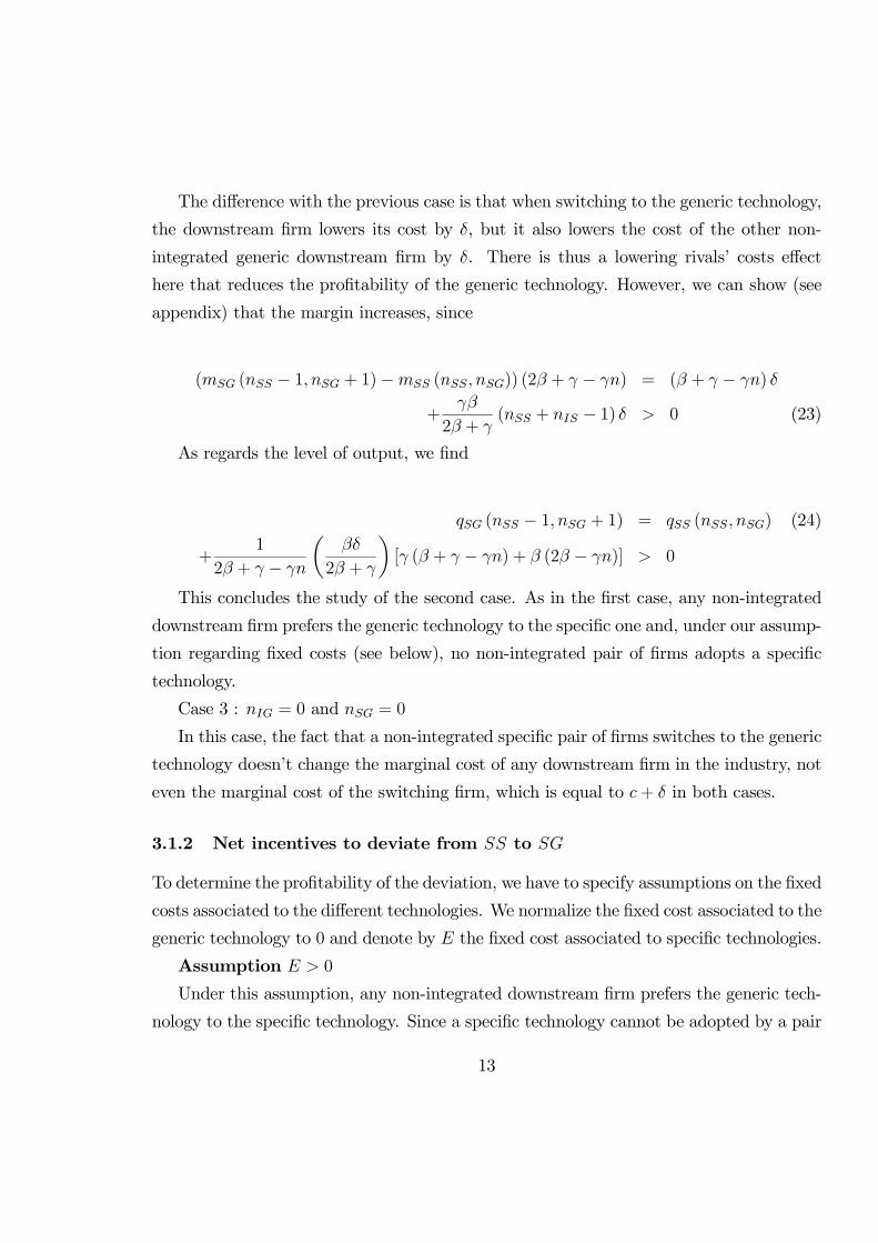
This concludes the study of the second case. As in the first case, any non-integrated

downstream firm prefers the generic technology to the specific one and, under our assump-

tion regarding fixed costs (see below), no non-integrated pair of firms adopts a specific

technology.

Case 3 : nIG = 0 and nSG = 0

In this case, the fact that a non-integrated specific pair of firms switches to the generic

technology doesn’t change the marginal cost of any downstream firm in the industry, not

even the marginal cost of the switching firm, which is equal to c+ δ in both cases.

3.1.2 Net incentives to deviate from SS to SG

To determine the profitability of the deviation, we have to specify assumptions on the fixed

costs associated to the different technologies. We normalize the fixed cost associated to the

generic technology to 0 and denote by E the fixed cost associated to specific technologies.

Assumption E > 0

Under this assumption, any non-integrated downstream firm prefers the generic tech-

nology to the specific technology. Since a specific technology cannot be adopted by a pair

13

of firms without the consent of the downstream firm, no pair of non-integrated firms adopts

a specific technology. In other words, it is necessary to integrate in order to achieve the

efficiency gains (in the sense of lower marginal costs) associated with a specific technology.

This is the sense of the proposition below.

Proposition 2 In equilibrium, nSS = 0.

It can be noted that this result holds as long as specific technologies are not associated

with significantly lower downstream fixed costs than the generic technology. It is only

in this case, that we don’t consider here, that efficiency gains can be achieved without

vertical integration.

3.2 The technological choice of integrated firms

We examine the incentives of integrated firms using the generic technology to switch

to a non-integrated structure (while keeping the generic technology). The structure of

marginal costs presented in table I shows that, in general, generic firms are indifferent

between integration and separation, since their profit (gross of any cost/benefit of vertical

integration not captured by the model) is the same in both cases. To avoid this indetermi-

nacy, we assume that there is a strictly positive cost of integration, so that firms strictly

prefer separation to integration. Since we don’t want to focus on these integration costs

that are not endogenous, we assume that they are very small.

There is one case, however, in which it is not indifferent in terms of gross profits for

generic firms to be integrated or not. It is when nIS = n− 1. Then, an integrated genericfirm has a downstream cost equal to c, whereas a separated downstream generic firm has

a cost equal to c+ δ. If we consider the joint profits of the pair of firms, the comparison

of integration and separation is ambiguous. This is because there is a strategic positive

effect on profits when the downstream firm is committed to a higher cost. There is thus

not necessarily in this case a supplementary profit to be shared between the upstream and

the downstream firms after a merger. We skip the analytical resolution that could allow

us to alleviate the indeterminacy, both because it is quite ackward and, more importantly,

because, as we said in the introduction, our focus in this paper is not on the strategic

14

effects that happen on the market (here, it is a residual market) when it is supplied by a

duopoly.

Proposition 3 In equilibrium, nIG = 0 or (nIS, nIG, nSG, nSS) = (n− 1, 1, 0, 0).

Proof Since we know that in equilibrium nSS = 0, we take this value as given.

We then have to show that, for any (nIS, nIG, nSG) 6= (n− 1, 1, 0) such that nIG ≥1, ΠIG (nIS, nIG, nSG) < ΠSG (nIS, nIG − 1, nSG + 1) . This is straightforward, given thevalues of costs given in table I and our assumptions concerning the costs of integration.

This proposition a partial result. It doesn’t fully describe the technological choice

of integrated firms in equilibrium. However, it is enough for our purpose in the present

section. In particular, it implies that, as well as there is no non-integrated pair of firms

using a specific technology, there is no integrated firm using the generic technology in an

equilibrium such that nSG ≥ 2, that is equilibria in which vertical foreclosure plays no

role. This is the type of equilibria that we focus on in the next section. We will thus focus

on situations in which it is equivalent to be integrated and to use a specific technology.

Since specific technologies are associated with lower marginal costs, vertical integration

increases the social surplus, as long as E is not to large.

4 Structural and technological choices in equilibrium

In this section, we provide a characterization of the equilibrium of the game defined in

section 2. Our main result concerns those equilibria that are such that nSG ≥ 3. It is

established in the first part of the section. In the second part of the section, we briefly

discuss other equilibria and the possibility of multiple equilibria.

4.0.1 Main result

Proposition 4 For any k ∈ {0; ...;n− 3}, there is a set of values of E such that

(nIS, nIG, nSS, nSG) = (k, 0, 0, n− k)

is an equilibrium and there is no other equilibrium satisfying nSG ≥ 3.

15

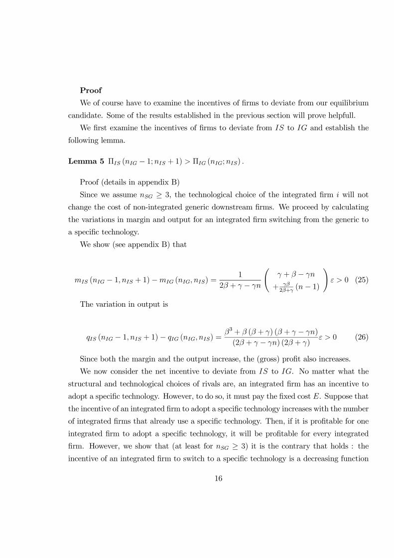
Proof

We of course have to examine the incentives of firms to deviate from our equilibrium

candidate. Some of the results established in the previous section will prove helpfull.

We first examine the incentives of firms to deviate from IS to IG and establish the

following lemma.

Lemma 5 ΠIS (nIG − 1;nIS + 1) > ΠIG (nIG;nIS) .

Proof (details in appendix B)

Since we assume nSG ≥ 3, the technological choice of the integrated firm i will not

change the cost of non-integrated generic downstream firms. We proceed by calculating

the variations in margin and output for an integrated firm switching from the generic to

a specific technology.

We show (see appendix B) that

mIS (nIG − 1, nIS + 1)−mIG (nIG, nIS) =1

2β + γ − γn

Ãγ + β − γn+ γβ2β+γ

(n− 1)

!ε > 0 (25)

The variation in output is

qIS (nIG − 1, nIS + 1)− qIG (nIG, nIS) = β3 + β (β + γ) (β + γ − γn)(2β + γ − γn) (2β + γ) ε > 0 (26)

Since both the margin and the output increase, the (gross) profit also increases.

We now consider the net incentive to deviate from IS to IG. No matter what the

structural and technological choices of rivals are, an integrated firm has an incentive to

adopt a specific technology. However, to do so, it must pay the fixed cost E. Suppose that

the incentive of an integrated firm to adopt a specific technology increases with the number

of integrated firms that already use a specific technology. Then, if it is profitable for one

integrated firm to adopt a specific technology, it will be profitable for every integrated

firm. However, we show that (at least for nSG ≥ 3) it is the contrary that holds : the

incentive of an integrated firm to switch to a specific technology is a decreasing function

16

of the number of integrated firms using a specific technology. In other words, the more

efficient competitors you have, the less profitable it is for you to become efficient as well.

We establish this result below.

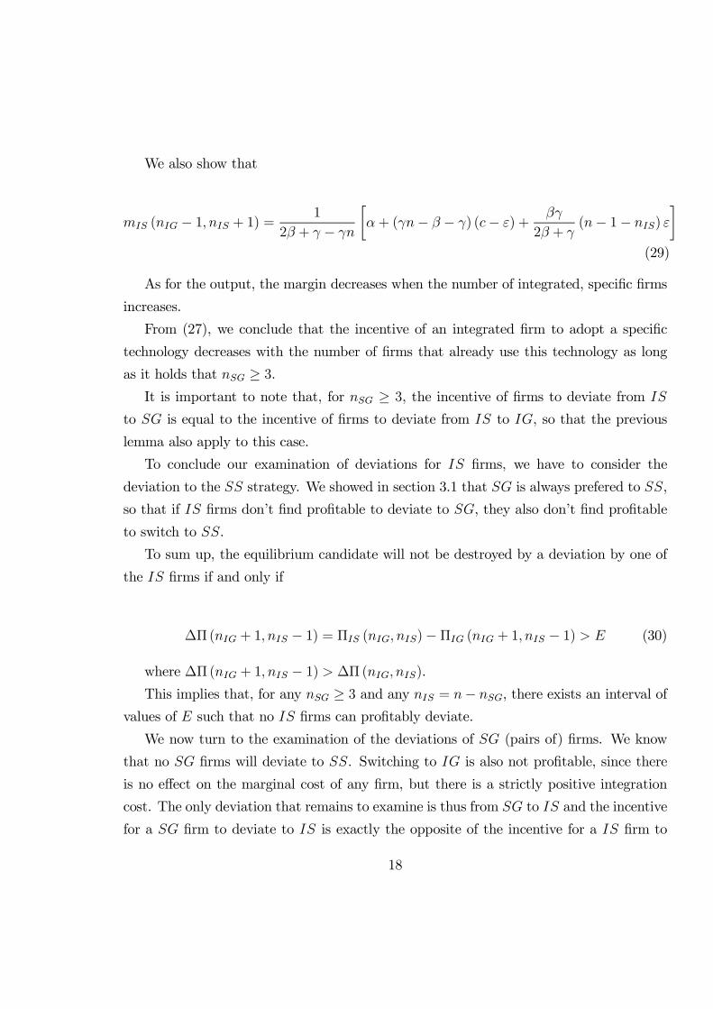
Definition 6 For any (nIG;nIS;nSG) ∈ {1; ...;n}×{0; ...;n}2 such that nIG+nIS+nSG =n, we define ∆Π (nIG, nIS) as the difference in an integrated firm’s gross profit with a

specific and with a generic technology, that is,

∆Π (nIG, nIS) = ΠIS (nIG − 1, nIS + 1)− ΠIG (nIG, nIS) .

Lemma 7 For nSG ≥ 3, ∆Π (nIG, nIS) < ∆Π (nIG + 1, nIS − 1).

Proof (details in appendix C)

We rewrite ∆Π (nIG, nIS) as

∆Π (nIG, nIS) = −ÃmIS (nIG − 1, nIS + 1)−mIG (nIG, nIS)

!ÃqIS (nIG − 1, nIS + 1)−qIG (nIG, nIS)

!(27)

+(mIS (nIG − 1, nIS + 1)−mIG (nIG, nIS)) qIS (nIG − 1, nIS + 1)+ (qIS (nIG − 1, nIS + 1)− qIG (nIG, nIS))mIS (nIG − 1, nIS + 1)

Since the variations in margin and output calculated above don’t depend on

(nIG;nIS;nSG), we just have to examine how these parameters influence

qIS (nIG − 1, nIS + 1) and mIS (nIG − 1, nIS + 1).We show (see appendix C) that

qIS (nIG − 1, nIS + 1) = α+1

2β + γ − γn

(α+ βc) (γn− β − γ)

+ β2β+γ

Ãβ (2β + γ)

+γ (β + γ) (1− n)

!ε

(28)− γβ2

(2β + γ − γn) (2β + γ)nISε

It is just the number nIS of integrated specific firms that influences qIS (nIG − 1, nIS + 1)and as it increases, qIS (nIG − 1, nIS + 1) decreases.

17

We also show that

mIS (nIG − 1, nIS + 1) = 1

2β + γ − γn·α+ (γn− β − γ) (c− ε) + βγ

2β + γ(n− 1− nIS) ε

¸(29)

As for the output, the margin decreases when the number of integrated, specific firms

increases.

From (27), we conclude that the incentive of an integrated firm to adopt a specific

technology decreases with the number of firms that already use this technology as long

as it holds that nSG ≥ 3.It is important to note that, for nSG ≥ 3, the incentive of firms to deviate from IS

to SG is equal to the incentive of firms to deviate from IS to IG, so that the previous

lemma also apply to this case.

To conclude our examination of deviations for IS firms, we have to consider the

deviation to the SS strategy. We showed in section 3.1 that SG is always prefered to SS,

so that if IS firms don’t find profitable to deviate to SG, they also don’t find profitable

to switch to SS.

To sum up, the equilibrium candidate will not be destroyed by a deviation by one of

the IS firms if and only if

∆Π (nIG + 1, nIS − 1) = ΠIS (nIG, nIS)− ΠIG (nIG + 1, nIS − 1) > E (30)

where ∆Π (nIG + 1, nIS − 1) > ∆Π (nIG, nIS).This implies that, for any nSG ≥ 3 and any nIS = n− nSG, there exists an interval of

values of E such that no IS firms can profitably deviate.

We now turn to the examination of the deviations of SG (pairs of) firms. We know

that no SG firms will deviate to SS. Switching to IG is also not profitable, since there

is no effect on the marginal cost of any firm, but there is a strictly positive integration

cost. The only deviation that remains to examine is thus from SG to IS and the incentive

for a SG firm to deviate to IS is exactly the opposite of the incentive for a IS firm to

18

deviate to SG discussed above. This means that there will be no profitable deviation

from the candidate equilibrium for any SG firm if and only if condition (30) is satisfied.

This completes the proof.

This result shows that (quite) any degree of vertical integration can be an equilibrium

in our model. This is not solely due to our assumption of a strictly positive fixed cost

associated with specific technologies, but more importantly to the fact that we do not

have the strategic complementarity found by McLaren (2000), but rather a strategic

substituability. When a pair of firms integrates, it lowers the profitability of integration

for other firms. In McLaren (2000), it rises this profitability. Strategic substituability

implies that when we observe a (vertical) merger wave in an industry, we have no reason

to expect that this merger wave will go on until vertical integration is generalized in the

industry. This result has important implications for antitrust policy that are discussed in

the next section.

4.0.2 Other equilibria

We discuss briefly here the other possible equilibria. Since the equilibrium (nIS, nIG, nSG) =

(n− 1, 1, 0) was discussed above, we focus on equilibria for which nIG = 0 and thus con-sider a pair (nIS, nSG) ∈ {0; ...;n} × {0; 1} such that nIS + nSG = n.First take nSG = 0. Vertical integration is complete in the industry. Depending on

E, it may or may not be profitable for one of the pair of firms to deviate to SG. The

particularity of this case is that the pair of firms may also find profitable to switch to

IG. However, if E is sufficiently low, nIS = n is an equilibrium. Essentially, as the

number of IS firms increases, it gets less and less profitable to be an IS firm, but it

remains profitable (even taking into account the fixed cost E) and full integration with

every integrated firm using a specific technology is an equilibrium.

Now take nSG = 1. Then, it may happen that the profitability of switching from IS

to SG first decreases when nIS increases from 0 to n− 2, but is higher when nIS = n− 2than when nIS = n− 3. Because of this, there may be a value of E such that none of theIS firms wants to switch to SG, but if one of them would do it, others may well follow

it and switch. If this non-monotonicity is not present, there may also exist a value of E

19

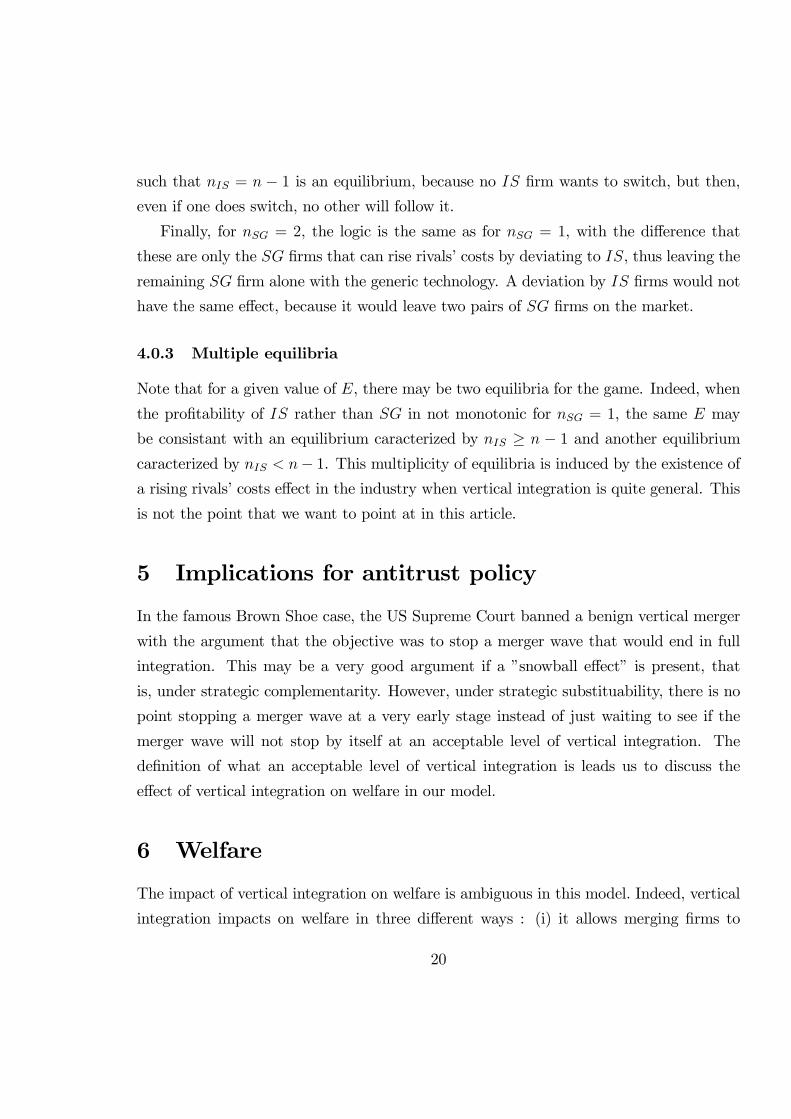
such that nIS = n − 1 is an equilibrium, because no IS firm wants to switch, but then,

even if one does switch, no other will follow it.

Finally, for nSG = 2, the logic is the same as for nSG = 1, with the difference that

these are only the SG firms that can rise rivals’ costs by deviating to IS, thus leaving the

remaining SG firm alone with the generic technology. A deviation by IS firms would not

have the same effect, because it would leave two pairs of SG firms on the market.

4.0.3 Multiple equilibria

Note that for a given value of E, there may be two equilibria for the game. Indeed, when

the profitability of IS rather than SG in not monotonic for nSG = 1, the same E may

be consistant with an equilibrium caracterized by nIS ≥ n − 1 and another equilibriumcaracterized by nIS < n− 1. This multiplicity of equilibria is induced by the existence ofa rising rivals’ costs effect in the industry when vertical integration is quite general. This

is not the point that we want to point at in this article.

5 Implications for antitrust policy

In the famous Brown Shoe case, the US Supreme Court banned a benign vertical merger

with the argument that the objective was to stop a merger wave that would end in full

integration. This may be a very good argument if a ”snowball effect” is present, that

is, under strategic complementarity. However, under strategic substituability, there is no

point stopping a merger wave at a very early stage instead of just waiting to see if the

merger wave will not stop by itself at an acceptable level of vertical integration. The

definition of what an acceptable level of vertical integration is leads us to discuss the

effect of vertical integration on welfare in our model.

6 Welfare

The impact of vertical integration on welfare is ambiguous in this model. Indeed, vertical

integration impacts on welfare in three different ways : (i) it allows merging firms to

20

achieve efficiency gains, which rises the welfare, (ii) it is associated with a fixed cost,

which reduces the welfare and (iii) it may be a rising rivals’ costs strategy, which reduces

the welfare. Even if we abstract from the third effect by focusing on merger waves that

stop before the number of separated firms is low enough for rising rivals’ costs effect to

play, one can see that there is no clearcut result on welfare. This indeterminacy is difficult

to avoid once we take into account both the efficiency gains associated to integration and

the costs associated to it.

7 Conclusion

Within the framework of a successive Bertrand oligopoly model, we establish a result

of strategic substituability that has strong implications both on the predictions of the

model and on the implications of the analysis for the antitrust policy. Concerning the

first point, we show that the degree of vertical integration in the model need not be either

0 or 100 percent, but can take quite any value, depending on the fixed cost associated

to specific technologies. In particular, it means that vertical merger waves may stop

before the industry is fully integrated. If this is the case, there is no foreclosure and no

rising rivals’ costs effect associated with vertical integration. Generalising the successive

duopoly models that are the basis of the literature on strategic vertical integration thus

leads to the conclusion that these models may well have exagerated the importance of the

foreclosure issue. Insofar as we can base antitrust recommendations on our model, these

would be in favor of a less severe control of vertical integration.

8 References

Avenel, E., 2000, Vertical integration, technological choice and foreclosure, Recherches

Economiques de Louvain, Vol. 66(3), 267-280.

Choi, J.P. and S.-S. Yi, 2000, Vertical foreclosure with the choice of input specifica-

tions, RAND Journal of Economics, Vol. 33(4), 717-743.

21

Church, J. and N. Gandal, 2000, Systems competition, vertical merger, and foreclosure,

Journal of Economics and Management Strategy, Vol. 9(1), 25-51.

McLaren, J., 2000, ”Globalization” and vertical structure, American Economic Re-

view, Vol. 90(5), 1239-1254.

Ordover, J.A., Saloner, G. and S.C. Salop, 1990, Equilibrium Vertical foreclosure,

American Economic Review, Vol. 80(1), 127-142.

Rosengren, E.S. and J.W. Jr. Meehan, 1994, Empirical evidence on vertical foreclo-

sure, Economic Inquiry, Vol. 32(2), 303-317.

Whinston, M.D., 2001, Assessing the property rights and transaction-cost theories of

firm scope, American Economics Review, Vol. 91(2), 184-188.

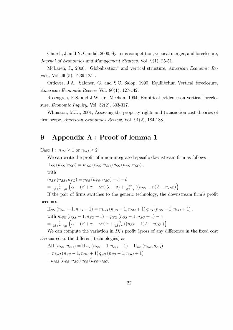
9 Appendix A : Proof of lemma 1

Case 1 : nIG ≥ 1 or nSG ≥ 2We can write the profit of a non-integrated specific downstream firm as follows :

ΠSS (nSS, nSG) = mSS (nSS, nSG) qSS (nSS, nSG) ,

with

mSS (nSS, nSG) = pSS (nSS, nSG)− c− δ= 1

2β+γ−γn³α− (β + γ − γn) (c+ δ) + γβ

2β+γ((nSS − n) δ − nISε)

´If the pair of firms switches to the generic technology, the downstream firm’s profit

becomes

ΠSG (nSS − 1, nSG + 1) = mSG (nSS − 1, nSG + 1) qSG (nSS − 1, nSG + 1) ,with mSG (nSS − 1, nSG + 1) = pSG (nSS − 1, nSG + 1)− c= 1

2β+γ−γn³α− (β + γ − γn) c + γβ

2β+γ((nSS − 1) δ − nISε)

´We can compute the variation in Di’s profit (gross of any difference in the fixed cost

associated to the different technologies) as

∆Π (nSS, nSG) = ΠSG (nSS − 1, nSG + 1)− ΠSS (nSS, nSG)= mSG (nSS − 1, nSG + 1) qSG (nSS − 1, nSG + 1)−mSS (nSS, nSG) qSS (nSS, nSG)

22

=

ÃmSG (nSS − 1, nSG + 1)

−mSS (nSS, nSG) +mSS (nSS, nSG)

!ÃqSG (nSS − 1, nSG + 1)

−qSS (nSS, nSG) + qSS (nSS, nSG)

!−mSS (nSS, nSG) qSS (nSS, nSG)

= (mSG (nSS − 1, nSG + 1)−mSS (nSS, nSG)) (qSG (nSS − 1, nSG + 1)− qSS (nSS, nSG))+ (mSG (nSS − 1, nSG + 1)−mSS (nSS, nSG)) qSS (nSS, nSG)

+ (qSG (nSS − 1, nSG + 1)− qSS (nSS, nSG))mSS (nSS, nSG)

Since quantities and margins are positive,

∆Π (nSS, nSG) > 0 if and only if mSG (nSS − 1, nSG + 1) − mSS (nSS, nSG) > 0 and

qSG (nSS − 1, nSG + 1)− qSS (nSS, nSG) > 0.We now show that both the variation in margin and in output are positive.

mSG (nSS − 1, nSG + 1)−mSS (nSS, nSG)

= 12β+γ−γn

³α− (β + γ − γn) c + γβ

2β+γ((nSS − 1) δ − nISε)

´− 12β+γ−γn

³α− (β + γ − γn) (c+ δ) + γβ

2β+γ((nSS − n) δ − nISε)

´=³β+γ−γn2β+γ−γn +

γβ(n−1)(2β+γ−γn)(2β+γ)

´δ > 0

qSG (nSS − 1, nSG + 1) = α+ (γnSG − β) pSG (nSS − 1, nSG + 1)+γnIGpIG (nSS − 1, nSG + 1) + γ (nSS − 1) pSS (nSS − 1, nSG + 1)+γnISpIS (nSS − 1, nSG + 1)Since pIG (nSS − 1, nSG + 1) = pSG (nSS − 1, nSG + 1),qSG (nSS − 1, nSG + 1) = α+ (γnSG + γnIG − β) pSG (nSS − 1, nSG + 1)+γ (nSS − 1) pSS (nSS − 1, nSG + 1) + γnISpIS (nSS − 1, nSG + 1)We now use the fact that

pIG (nSS − 1, nSG + 1) = pIG (nSS, nSG)− γβ(2β+γ−γn)(2β+γ)δ,

pSS (nSS − 1, nSG + 1) = pSS (nSS, nSG)− γβ(2β+γ−γn)(2β+γ)δ

and

pIS (nSS − 1, nSG + 1) = pIS (nSS, nSG)− γβ(2β+γ−γn)(2β+γ)δ

to rewrite qSG (nSS − 1, nSG + 1) asqSG (nSS − 1, nSG + 1) = α+ (γnSG + γnIG − β) pSG (nSS, nSG)+γ (nSS − 1) pSS (nSS, nSG) + γnISpIS (nSS, nSG) + γβ(β+γ−γn)

(2β+γ−γn)(2β+γ)δ

Rearranging the terms leads to

qSG (nSS − 1, nSG + 1) = α+ (γnSG + γnIG) pSG (nSS, nSG)

23

+(γnSS − γ − β) pSS (nSS, nSG) + γnISpIS (nSS, nSG)− βpSG (nSS, nSG)+βpSS (nSS, nSG) +

γβ(β+γ−γn)(2β+γ−γn)(2β+γ)δ

and finally to

qSG (nSS − 1, nSG + 1) = qSS (nSS, nSG) + β [pSS (nSS, nSG)− pSG (nSS, nSG)]+ 12β+γ−γn

³βγ2β+γ

´(β + γ − γn) δ

Since

pSS (nSS, nSG)− pSG (nSS, nSG) = βδ2β+γ

> 0,

every term on the right-hand side is positive and

qSG (nSS − 1, nSG + 1)− qSS (nSS, nSG) > 0.Case 2 : nIG = 0 and nSG = 1

We proceed as in the previous case to establish that

∆Π (nSS, nSG) > 0 if and only if mSG (nSS − 1, nSG + 1) − mSS (nSS, nSG) > 0 and

qSG (nSS − 1, nSG + 1)− qSS (nSS, nSG) > 0.mSG (nSS − 1, nSG + 1)−mSS (nSS, nSG)

= 12β+γ−γn

³α− (β + γ − γn) c + γβ

2β+γ((nSS − 1) δ − nISε)

´− 12β+γ−γn

³α− (β + γ − γn) (c+ δ)− γβ

2β+γnIS (δ + ε)

´=³β+γ−γn2β+γ−γn +

γβ(nSS+nIS−1)(2β+γ−γn)(2β+γ)

´δ

=³β+γ−γn2β+γ−γn +

γβ(n−2)(2β+γ−γn)(2β+γ)

´δ > 0

qSS (nSS, nSG) = α− βpSS (nSS, nSG) + γ (nSS − 1) pSS (nSS, nSG)+γnISpIS (nSS, nSG) + γnSGpSG (nSS, nSG)

= α+ (γnSS − γ − β) pSS (nSS, nSG) + γnISpIS (nSS, nSG)+γnSGpSG (nSS, nSG)

qSG (nSS − 1, nSG + 1) = α− βpSG (nSS − 1, nSG + 1)+γ (nSS − 1) pSS (nSS − 1, nSG + 1) + γnISpIS (nSS − 1, nSG + 1)+γnSGpSG (nSS − 1, nSG + 1)= α+ (γnSG − β) pSG (nSS − 1, nSG + 1) + γ (nSS − 1) pSS (nSS − 1, nSG + 1)+γnISpIS (nSS − 1, nSG + 1)= α+ γnSGpSG (nSS − 1, nSG + 1) + (γnSS − γ − β) pSS (nSS − 1, nSG + 1)+γnISpIS (nSS − 1, nSG + 1)

24

+β (pSS (nSS − 1, nSG + 1)− pSG (nSS − 1, nSG + 1))= qSS (nSS, nSG) + (γnSS − γ − β) [pSS (nSS − 1, nSG + 1)− pSS (nSS, nSG)]+γnIS [pIS (nSS − 1, nSG + 1)− pIS (nSS, nSG)]+γnSG [pSG (nSS − 1, nSG + 1)− pSG (nSS, nSG)]+β [pSS (nSS − 1, nSG + 1)− pSG (nSS − 1, nSG + 1)]We now calculate the terms in square brackets.

pSS (nSS − 1, nSG + 1)− pSS (nSS, nSG)= 1

2β+γ−γn³α+ β (c+ δ) + γβ

2β+γ(− (nIS + nSG + 1) δ − nISε)

´− 12β+γ−γn

³α+ β (c+ δ)− γβ

2β+γnIS (ε+ δ)

´= − γβ

(2β+γ)(2β+γ−γn) (nSG + 1) δ

pIS (nSS − 1, nSG + 1)− pIS (nSS, nSG)= 1

2β+γ−γn³α+ β (c− ε) + γβ

2β+γ((nSS − 1) δ + (nSS + nSG) ε)

´− 12β+γ−γn

³α+ β (c− ε) + γβ

2β+γ(nSS + nSG) (ε+ δ)

´= − γβ

(2β+γ)(2β+γ−γn) (nSG + 1) δ

pSG (nSS − 1, nSG + 1)− pSG (nSS, nSG)= 1

2β+γ−γn³α+ βc+ γβ

2β+γ((nSS − 1) δ − nISε)

´− 12β+γ−γn

³α+ β (c+ δ)− γβ

2β+γnIS (δ + ε)

´= − β

2β+γ−γnδ +γβ

(2β+γ)(2β+γ−γn) (nSS + nIS − 1) δ= − β

2β+γ−γnδ +γβ

(2β+γ)(2β+γ−γn) (n− 2) δpSS (nSS − 1, nSG + 1)− pSG (nSS − 1, nSG + 1)= 1

2β+γ−γn³α+ β (c+ δ) + γβ

2β+γ(− (nIS + nSS + 1) δ − nISε)

´− 12β+γ−γn

³α+ βc+ γβ

2β+γ((nSS − 1) δ − nISε)

´= βδ

2β+γ−γn − γβ(2β+γ)(2β+γ−γn)nδ

Using these expressions, we calculate the variation in output as

qSG (nSS − 1, nSG + 1)− qSS (nSS, nSG)

= 12β+γ−γn

(γnSS − γ − β) γβ

(2β+γ)(−nSG − 1) δ

+γnISγβ

(2β+γ)(−nSG − 1) δ + γnSG

h−βδ + γβ

(2β+γ)(n− 2) δ

i+β2δ − γβ2

(2β+γ)nδ

Simplifying this expression, taking into account the fact that nSG = 1, leads to

25

qSG (nSS − 1, nSG + 1)− qSS (nSS, nSG)= 1

2β+γ−γnh− γβ(2β+γ)

(n− 2) (γ + β) + β (β − γ)iδ

Since the sign of the term in square brackets is not a priori evident, we rewrite it as

follows :

− γβ(2β+γ)

(n− 2) (γ + β) + β (β − γ)= β

(2β+γ)

£γ2 (1− n) + βγ (1− n) + 2β2¤

= β(2β+γ)

γ (β + γ − γn)| {z }> 0

+β (β + γ − γn)| {z }

> 0+β (β − γ)| {z }> 0

We thus proved that

qSG (nSS − 1, nSG + 1)− qSS (nSS, nSG) > 0.This completes the proof.

10 Appendix B : Proof of lemma 6

We proceed as for proposition 1, so that proving proposition 2 is just the same as proving

that(mIS (nIG − 1, nIS + 1)−mIG (nIG, nIS) > 0

qIS (nIG − 1, nIS + 1)− qIG (nIG, nIS) > 0Case 1 : nIG 6= 1;nSG 6= 1mIS (nIG − 1, nIS + 1)−mIG (nIG, nIS)

= pIS (nIG − 1, nIS + 1)− (c− ε)− (pIG (nIG, nIS)− c)= 1

2β+γ−γn³α− (β + γ − γn) (c− ε) + γβ

2β+γ(nIG + nSG − 1) ε

´− 12β+γ−γn

³α− (β + γ − γn) c− γβ

2β+γnISε

´= 1

2β+γ−γn³(β + γ − γn) ε+ γβ

2β+γ(nIG + nSG + nIS − 1) ε

´= 1

2β+γ−γn³β + γ − γn+ γβ

2β+γ(n− 1)

´ε > 0

qIG (nIG, nIS) = α+ (γnIG − γ − β) pIG (nIG, nIS)+γnISpIS (nIG, nIS) + γnSGpSG (nIG, nIS)

qIS (nIG − 1, nIS + 1) = α+ (γnIS − β) pIS (nIG − 1, nIS + 1)+ (γnIG − γ) pIG (nIG − 1, nIS + 1) + γnSGpSG (nIG − 1, nIS + 1)qIS (nIG − 1, nIS + 1)− qIG (nIG, nIS)

26

= γnSG

"pSG (nIG − 1, nIS + 1)−pSG (nIG, nIS)

#+ γnIS

"pIS (nIG − 1, nIS + 1)−pIS (nIG, nIS)

#+(γnIG − γ − β) [pIG (nIG − 1, nIS + 1)− pIG (nIG, nIS)]+β [pIS (nIG − 1, nIS + 1)− pIG (nIG − 1, nIS + 1)]Replacing the terms in square brackets with their expression, we show that :

qIS (nIG − 1, nIS + 1)− qIG (nIG, nIS)= 1

2β+γ−γnn(β + γ − γn) γβ

2β+γε+ β2ε− γβ2

2β+γnεo

qIS (nIG − 1, nIS + 1)− qIG (nIG, nIS) = β(β+γ−γn)(β+γ)+β3(2β+γ−γn)(2β+γ) ε > 0

This completes the proof.

11 Appendix C : Proof of lemma 8

mIS (nIG − 1, nIS + 1) = pIS (nIG − 1, nIS + 1)− (c− ε)= 1

2β+γ−γn³α− (β + γ − γn) (c− ε) + γβ

2β+γ(nIG + nSG − 1) ε

´= 1

2β+γ−γn³α− (β + γ − γn) (c− ε) + γβ

2β+γ(n− 1) ε− γβ

2β+γnISε

´=⇒ ∂

∂nISmIS (nIG − 1, nIS + 1) < 0

qIS (nIG − 1, nIS + 1) = α+ (γnIS − β) pIS (nIG − 1, nIS + 1)+ (γnIG − γ) pIG (nIG − 1, nIS + 1) + γnSGpSG (nIG − 1, nIS + 1)= α+ (γnIS − β) pIS (nIG − 1, nIS + 1)+ (γnIG + γnSG − γ) pIG (nIG − 1, nIS + 1)= α+ (γnIS−β)(α+βc−βε)

2β+γ−γn + (γnIG+γnSG−γ)(α+βc)2β+γ−γn

+ γnIS−β2β+γ−γn

γβ2β+γ

(nIG + nSG − 1) ε− (γnIG+γnSG−γ)2β+γ−γn

γβ2β+γ

(nIS + 1) ε

= α+ 12β+γ−γn

£(γn− β − γ) (α+ βc) + β2ε− γnISβε

¤+ 12β+γ−γn

γβ2β+γ

[(γnIS − β)− γ (nIS + 1)] (n− nIS − 1) ε= α+ 1

2β+γ−γn£(γn− β − γ) (α+ βc) + β2ε− γnISβε

¤− 12β+γ−γn

γβ2β+γ

(β + γ) (n− nIS − 1) ε= α+ 1

2β+γ−γnh(γn− β − γ) (α+ βc) + β2ε− γβ

2β+γ(β + γ) (n− 1) ε

i+ 12β+γ−γn

h−γβ + γβ

2β+γ(β + γ)

inISε

27

= α+ 12β+γ−γn

((γn− β − γ) (α+ βc)

+ β2β+γ

[β (2β + γ)− γ (β + γ) (n− 1)] ε

)− γβ2

(2β+γ−γn)(2β+γ)nISε

=⇒ ∂∂nIS

qIS (nIG − 1, nIS + 1) < 0This completes the proof.

28