Stratigraphic Elastic Inversion for Seismic Lithology Discrimination in a Turbiditic Reservoir J-P Coulon*, Y. Lafet, B. Deschizeaux, P.M. Doyen and P. Duboz, Compagnie Générale de Géophysique Summary An integrated workflow, including careful seismic data conditioning, pre-stack elastic inversion and seismic lithology classification has been applied to predict the distribution of channel sands in a complex turbiditic reservoir. Three partial stacks, with angles in the range 8-50 degrees, have been calibrated using elastic logs at three well locations. A well-based feasibility shows that reservoir sands can in theory be identified from a cross plot of Poisson’s ratio versus P-wave impedance. In practice, seismic lithology discrimination is challenging due to a complex AVA response, which is affected by the difference in seismic frequency content between near and ultra far angles. Our simultaneous elastic inversion procedure is able to account for the angle-dependent change in seismic bandwidth and delivers high-resolution estimates of both P- and S-wave impedances, which have been used to calculate a sand lithology cube. The inversion was performed in a layered stratigraphic framework that has been automatically extracted from seismic dip information. This has yielded 3-D images of reservoir elastic properties that better conform to the complex shapes of the channelized sand deposits. Introduction Development of turbiditic reservoirs presents significant technical challenges. In particular, assessment of the lateral and vertical connectivity between channel sands usually requires high-resolution, large offset 3-D seismic data acquisition, and careful application of pre-stack inversion techniques for lithology and fluid prediction. Experience shows that acoustic impedance is usually not a good lithology predictor. In the context of our field example, Figure 1 shows a well log-based cross-plot of Poisson’s ratio versus P-wave acoustic impedance (Ip), colour-coded according to the shale volume fraction (Vsh). It clearly shows that acoustic impedance alone cannot be used to discriminate sands but that Poisson’s ratio is a good sand indicator, as shown by the polygon. This observation motivated the application of a pre-stack elastic inversion in this project. Input seismic data at 12.5m CDP spacing consist of three angles stacks: near (12-20°), far (20-36) and ultra far (36-60°). Three wells with elastic and lithology logs are available for calibration in the 5km x 7km project area. The inversion window is 800msec long and contains several reservoir intervals. The main difficulties to be tackled by the inversion workflow were as follows:

• Only three interpreted horizons are available to constrain the stratigraphic model in the long inversion window.

• There is a significant degradation of frequency content from near to ultra far angles, with the dominant frequency dropping from about 25Hz to 15Hz.

• Seismic event correlations between near and ultra far stacks are poor. These weak correlations may be due to AVA effects, complicated by the angle-dependent seismic bandwidth but may also relate to imperfect NMO corrections in the partial stack generation.

• The data exhibit a high level of organized noise (diffracted multiples) that increases with depth.

• Good estimation of Poisson’s ratio is required to discriminate the reservoir sands.

The inversion workflow was customized to address the above challenges, with particular attention to seismic data pre-conditioning, well-based extraction of angle-dependent wavelets, building of a layered initial model consistent with the complex seismic stratigraphy, well calibration of the inverted Ip – PR cross plot and extraction of a lithology cube that can be used for planning new well trajectories.

Fig 1. Poisson’s Ratio versus Ip, coloured from Vsh, with sand attribute polygon. Points represent log data sampled at 1msec from three wells.

3000 11000

0

0.44

Poi

sson

’s R

atio

Ip

0% 100%Vsh

Ip

0% 100%Vsh

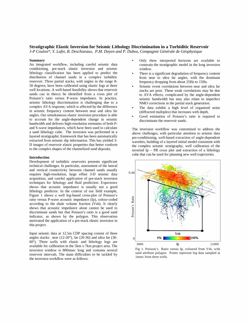
Stratigraphic Elastic Inversion for Seismic Lithology Discrimination

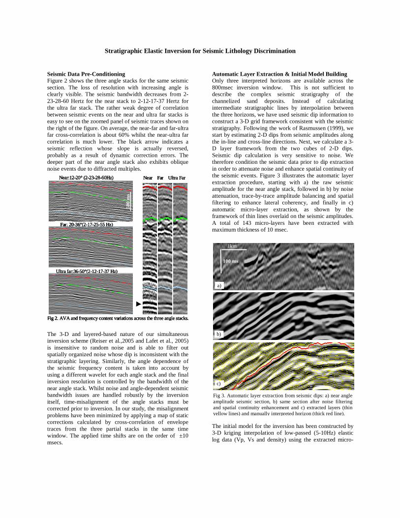
Seismic Data Pre-Conditioning Figure 2 shows the three angle stacks for the same seismic section. The loss of resolution with increasing angle is clearly visible. The seismic bandwidth decreases from 2-23-28-60 Hertz for the near stack to 2-12-17-37 Hertz for the ultra far stack. The rather weak degree of correlation between seismic events on the near and ultra far stacks is easy to see on the zoomed panel of seismic traces shown on the right of the figure. On average, the near-far and far-ultra far cross-correlation is about 60% whilst the near-ultra far correlation is much lower. The black arrow indicates a seismic reflection whose slope is actually reversed, probably as a result of dynamic correction errors. The deeper part of the near angle stack also exhibits oblique noise events due to diffracted multiples.

The 3-D and layered-based nature of our simultaneous inversion scheme (Reiser et al.,2005 and Lafet et al., 2005) is insensitive to random noise and is able to filter out spatially organized noise whose dip is inconsistent with the stratigraphic layering. Similarly, the angle dependence of the seismic frequency content is taken into account by using a different wavelet for each angle stack and the final inversion resolution is controlled by the bandwidth of the near angle stack. Whilst noise and angle-dependent seismic bandwidth issues are handled robustly by the inversion itself, time-misalignment of the angle stacks must be corrected prior to inversion. In our study, the misalignment problems have been minimized by applying a map of static corrections calculated by cross-correlation of envelope traces from the three partial stacks in the same time window. The applied time shifts are on the order of ±10 msecs.

Automatic Layer Extraction & Initial Model Building Only three interpreted horizons are available across the 800msec inversion window. This is not sufficient to describe the complex seismic stratigraphy of the channelized sand deposits. Instead of calculating intermediate stratigraphic lines by interpolation between the three horizons, we have used seismic dip information to construct a 3-D grid framework consistent with the seismic stratigraphy. Following the work of Rasmussen (1999), we start by estimating 2-D dips from seismic amplitudes along the in-line and cross-line directions. Next, we calculate a 3-D layer framework from the two cubes of 2-D dips. Seismic dip calculation is very sensitive to noise. We therefore condition the seismic data prior to dip extraction in order to attenuate noise and enhance spatial continuity of the seismic events. Figure 3 illustrates the automatic layer extraction procedure, starting with a) the raw seismic amplitude for the near angle stack, followed in b) by noise attenuation, trace-by-trace amplitude balancing and spatial filtering to enhance lateral coherency, and finally in c) automatic micro-layer extraction, as shown by the framework of thin lines overlaid on the seismic amplitudes. A total of 143 micro-layers have been extracted with maximum thickness of 10 msec. The initial model for the inversion has been constructed by 3-D kriging interpolation of low-passed (5-10Hz) elastic log data (Vp, Vs and density) using the extracted micro-

Fig 3. Automatic layer extraction from seismic dips: a) near angle amplitude seismic section, b) same section after noise filtering and spatial continuity enhancement and c) extracted layers (thin yellow lines) and manually interpreted horizon (thick red line).

a)

b)

c)

1km

100 ms

Fig 2. AVA and frequency content variations across the three angle stacks.

Near:12-20° (2-23-28-60Hz) Near Far Ultra Far

Far: 20-36°(2-17-25-55 Hz)

Ultra far:36-50°(2-12-17-37 Hz)

500

ms

Fig 2. AVA and frequency content variations across the three angle stacks.

Near:12-20° (2-23-28-60Hz) Near Far Ultra Far

Far: 20-36°(2-17-25-55 Hz)

Ultra far:36-50°(2-12-17-37 Hz)

500

ms

Fig 2. AVA and frequency content variations across the three angle stacks.

Near:12-20° (2-23-28-60Hz) Near Far Ultra Far

Far: 20-36°(2-17-25-55 Hz)

Ultra far:36-50°(2-12-17-37 Hz)

500

ms

Stratigraphic Elastic Inversion for Seismic Lithology Discrimination

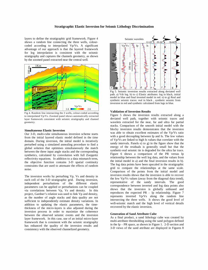
layers to define the stratigraphic grid framework. Figure 4 shows a random line connecting the three wells, colour-coded according to interpolated Vp/Vs. A significant advantage of our approach is that the layered framework for log interpolation is consistent with the seismic stratigraphy and captures the channels geometry, as shown by the zoomed panel extracted near the central well.

Simultaneous Elastic Inversion Our 3-D, multi-cube simultaneous inversion scheme starts from the initial layered elastic model defined in the time domain. During inversion, the initial model is iteratively perturbed using a simulated annealing procedure to find a global solution that optimises simultaneously the match between the three input angle stacks and the corresponding synthetics, calculated by convolution with full Zoeppritz reflectivity equations. In addition to a data mismatch term, the objective function contains 3-D spatial continuity constraints that are used to attenuate the effects of random noise. The inversion works by perturbing Vp, Vs and density in each cell of the 3-D stratigraphic grid. During inversion, independent perturbations of the different elastic parameters can be applied or perturbations can be coupled via correlations between Vp, Vs and density. In this project, Gardner’s relation was used to link Vp and density, as the number of angle stacks and data quality are not sufficient to independently estimate density variations. In addition to updating the elastic parameters, the time-thickness of the micro-layers is also adjusted during the inversion process in order to maximize the coherence between the observed seismic events and the inversion layer framework. In this case, use of an initial micro-layer framework that is consistent with the seismic stratigraphy has enhanced the quality of the inversion results and consistency with the observed channelized geometry.

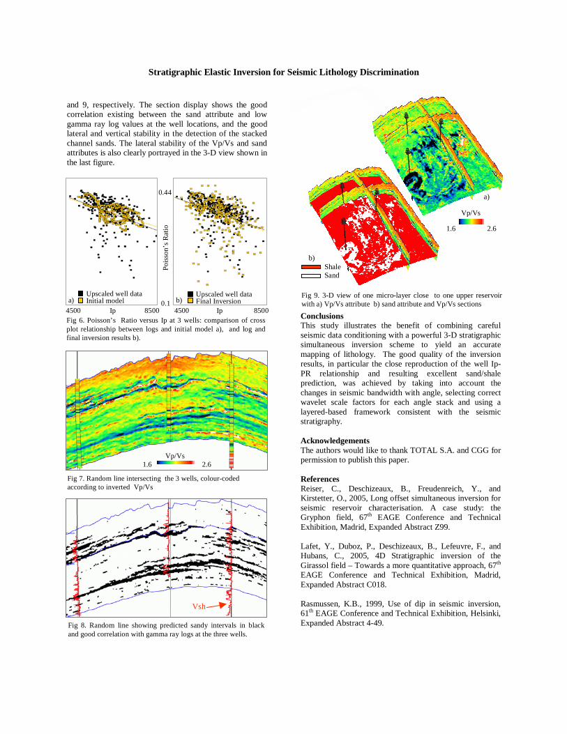
Validation of Inversion Results Figure 5 shows the inversion results extracted along a deviated well path, together with seismic traces and wavelets extracted for the near, far and ultra far partial stacks. Comparison of the smooth initial model with the blocky inversion results demonstrates that the inversion was able to obtain excellent estimates of the Vp/Vs ratio with a good decoupling between Ip and Is. The low values of Vp/Vs are linked to high Is values that correlate with the sandy intervals. Panels e) to g) in the figure show that the energy of the residuals is generally small but that the synthetic-real seismic tie is degraded for the ultra far trace. Figure 6 shows a comparison of the PR versus Ip relationship between the well log data, and the values from the initial model in a) and the final inversion results in b). The log data points have been upscaled in the stratigraphic grid to compare the relationships at the same scale. Comparison of the points from the initial model and inversion results shows that the inversion is able to recover the low Vp/Vs values (away from the diagonal data trend), representative of the sandy intervals. The good correspondence between inverted and log data points also shows that the inversion is globally unbiased and reproduces the expected PR – Ip relationship. Figure 7 represents inverted Vp/Vs along the random line intersecting the three wells. It shows the good level of well-seismic match and the high level of vertical details recovered by the elastic inversion. Generation of Sand Attribute Cube As a final product, a sand lithology cube was created by multi-attribute thresholding using the sand polygon defined in the Ip – PR space, as shown in Figure 1. 2-D section and 3-D views of the sand attribute are displayed in Figures 8

Fig 4. Random line intersecting the 3 wells, colour-coded according to interpolated Vp/Vs. Zoomed panel shows automatically extracted layer framework consistent with seismic stratigraphy and channel geometry.

100

ms 1Km

Vp/Vs1.6 2.6

50 m

s

Seismic wavelets

Fig 5. Seismic inversion results extracted along deviated well path. a) Vsh log. b) to c) Elastic attributes: log in black, initial model in blue and final inverted model in red. e) to g) Real andsynthetic seismic traces: real in black , synthetic seismic frominversion in red and synthetic calculated from logs in blue.

Ip Is36-60°20-36°12-20°

a b c d e f g

100

ms

Vp/Vs

Stratigraphic Elastic Inversion for Seismic Lithology Discrimination

and 9, respectively. The section display shows the good correlation existing between the sand attribute and low gamma ray log values at the well locations, and the good lateral and vertical stability in the detection of the stacked channel sands. The lateral stability of the Vp/Vs and sand attributes is also clearly portrayed in the 3-D view shown in the last figure.

Conclusions This study illustrates the benefit of combining careful seismic data conditioning with a powerful 3-D stratigraphic simultaneous inversion scheme to yield an accurate mapping of lithology. The good quality of the inversion results, in particular the close reproduction of the well Ip-PR relationship and resulting excellent sand/shale prediction, was achieved by taking into account the changes in seismic bandwidth with angle, selecting correct wavelet scale factors for each angle stack and using a layered-based framework consistent with the seismic stratigraphy. Acknowledgements The authors would like to thank TOTAL S.A. and CGG for permission to publish this paper. References Reiser, C., Deschizeaux, B., Freudenreich, Y., and Kirstetter, O., 2005, Long offset simultaneous inversion for seismic reservoir characterisation. A case study: the Gryphon field, 67th EAGE Conference and Technical Exhibition, Madrid, Expanded Abstract Z99. Lafet, Y., Duboz, P., Deschizeaux, B., Lefeuvre, F., and Hubans, C., 2005, 4D Stratigraphic inversion of the Girassol field – Towards a more quantitative approach, 67th EAGE Conference and Technical Exhibition, Madrid, Expanded Abstract C018. Rasmussen, K.B., 1999, Use of dip in seismic inversion, 61th EAGE Conference and Technical Exhibition, Helsinki, Expanded Abstract 4-49.

Fig 7. Random line intersecting the 3 wells, colour-coded according to inverted Vp/Vs

1.6 2.6Vp/Vs

Fig 8. Random line showing predicted sandy intervals in black and good correlation with gamma ray logs at the three wells.

Fig 6. Poisson’s Ratio versus Ip at 3 wells: comparison of cross plot relationship between logs and initial model a), and log and final inversion results b).

Pois

son’

sR

atio

Ip4500 8500 Ip0.1

0.44

4500 8500

Upscaled well data Final Inversionb)

Upscaled well data Initial model

Vsh

a)Fig 9. 3-D view of one micro-layer close to one upper reservoir with a) Vp/Vs attribute b) sand attribute and Vp/Vs sections

a)

Shale Sand

b)

Vp/Vs

1.6 2.6