Copyright in the design and typographical arrangement rests with One North East. This publication, excluding logos, may be reproducedfree of charge in any format or medium for research, private study or for internal circulation within an organisation. This is subject to itbeing reproduced accurately and not used in a misleading context.
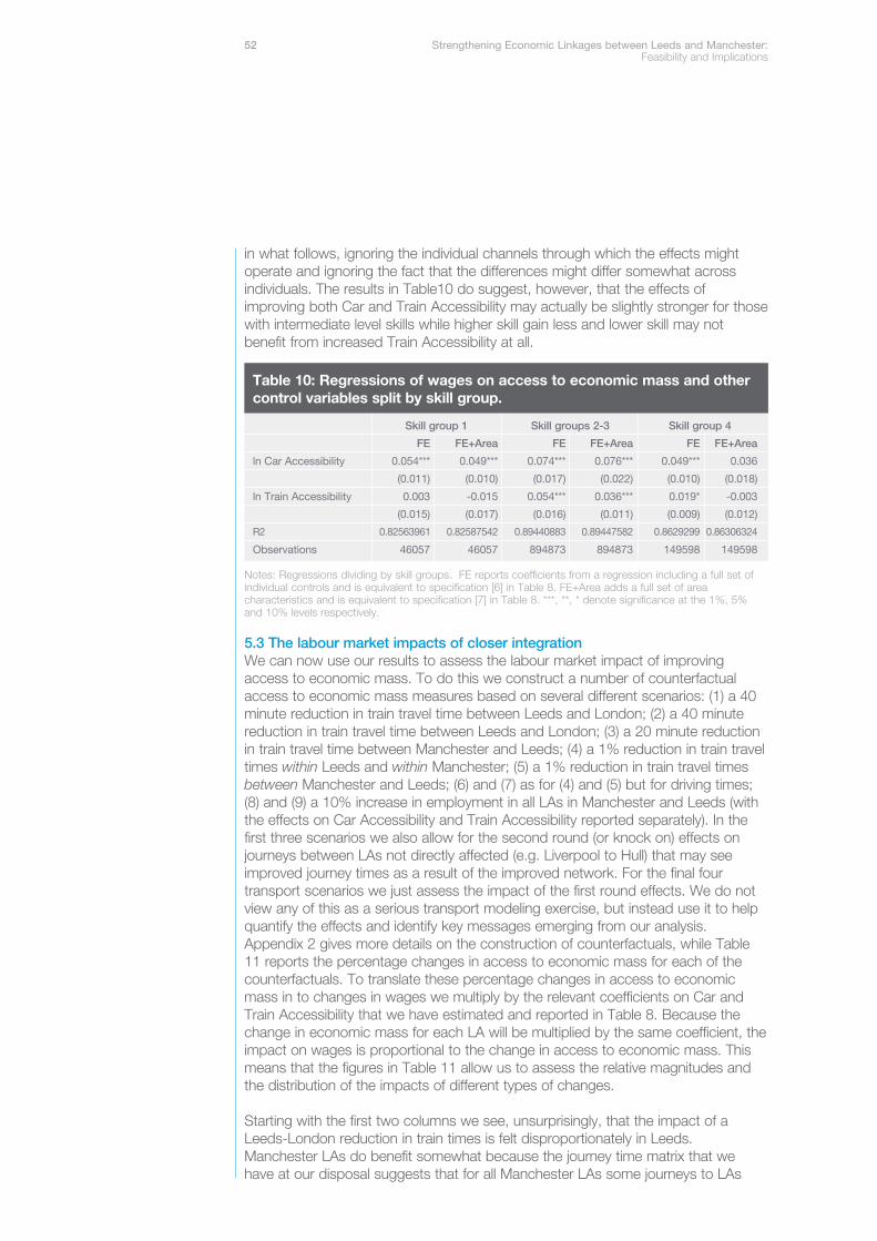
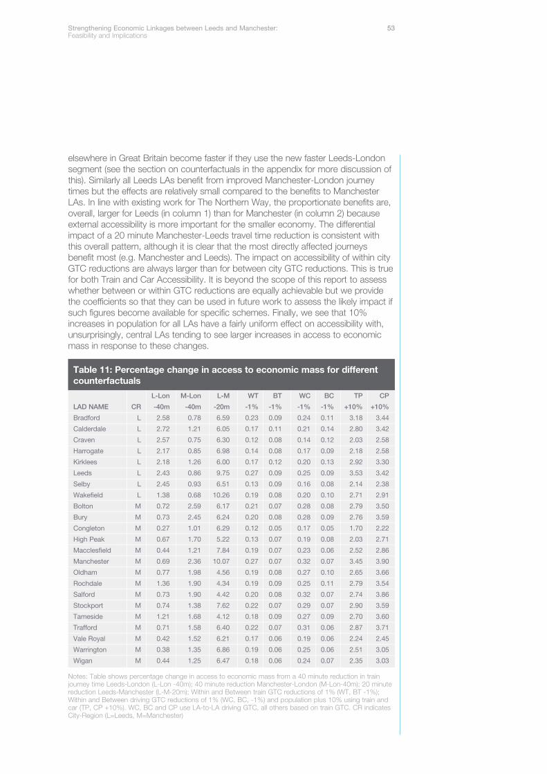
The material must be acknowledged as copyright One North East and the title of the publication specified.
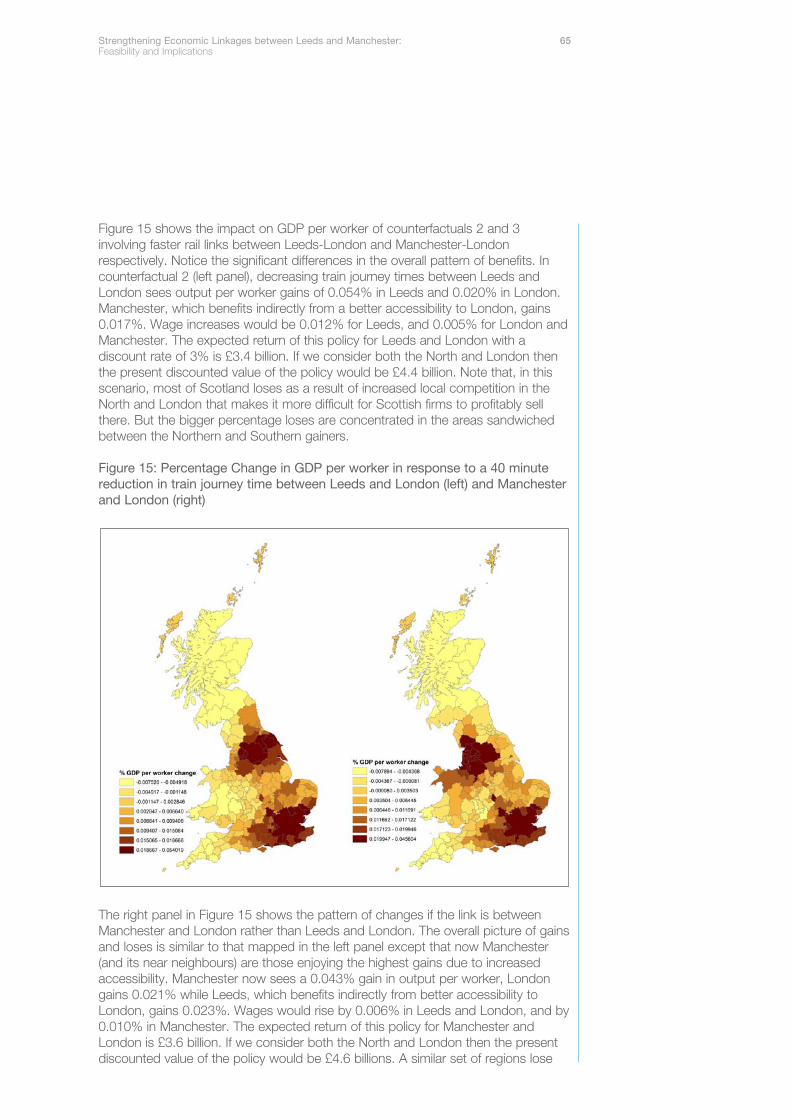
This work contains statistical data from ONS which is Crown copyright and reproduced with the permission of the controller of HMSOand Queen’s Printer for Scotland. The use of the ONS statistical data in this work does not imply the endorsement of the ONS in relationto the interpretation or analysis of the statistical data. This work uses research datasets which may not exactly reproduce NationalStatistics aggregates.
Copyright of the statistical results may not be assigned, and publishers of this data must have or obtain a licence from HMSO. The ONSdata in these results are covered by the terms of the standard HMSO “click-use” licence. We thank Lizze Diss at the Department forTransport and Dan Graham at Imperial College London for their help with the ward to ward GTC for driving. We thank We thank PeterWiener at Steer Davies Gleeve and John Jarvis at Yorkshire Forward for advice on constructing the train counterfactuals.
This research programme was delivered by theSpatial Economics Research Centre (SERC)and was commissioned and sponsored by The Northern Way.
The SERC team, based at the London School ofEconomics comprised:
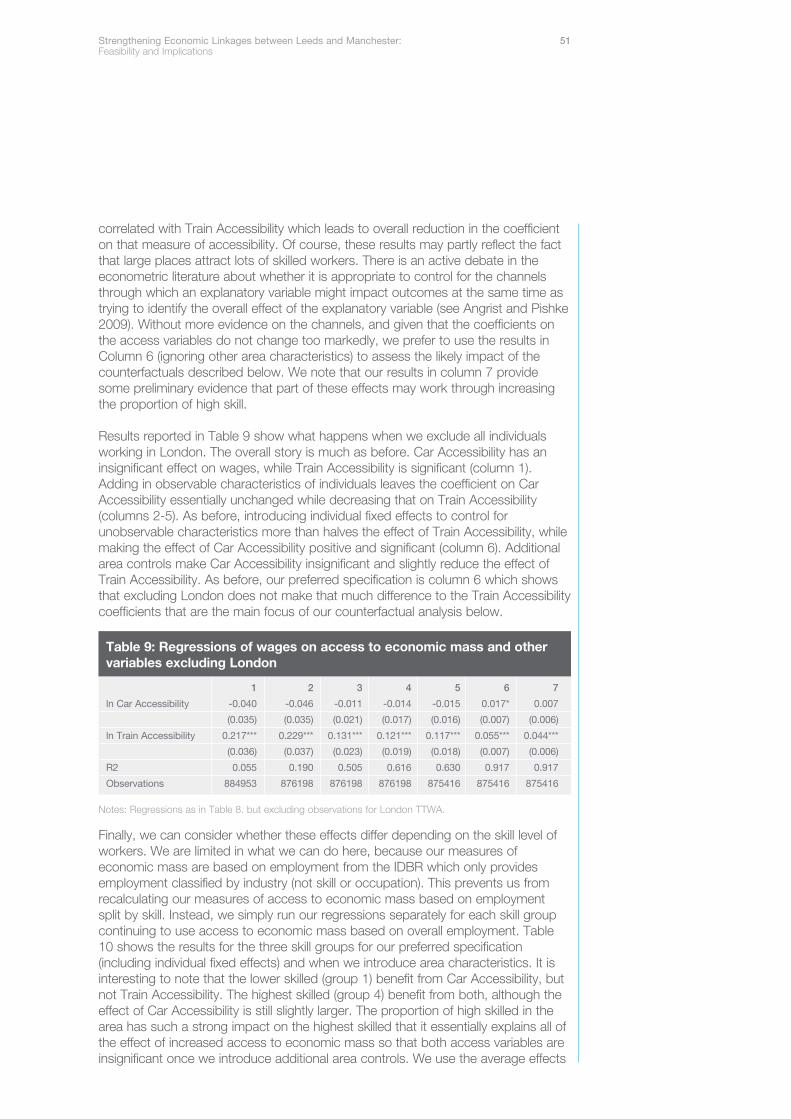
Henry Overman (LSE and SERC)Steve Gibbons (LSE and SERC)Sabine D’Costa (LSE and SERC)Giordano Mion (LSE and SERC)Panu Pelkonen (LSE and SERC)Guilherme Resende (LSE and SERC)Mike Thomas (LSE and SERC)
A Steering Group supported the implementation ofthe research programme, and policy implicationswere informed by discussions at a PolicyReference Group.
The following contributed to the work of thesegroups:
Department of Business, Innovation and Skills: Adrien Amzallag, Andrew Cunningham-Hughes
Department of Communities and LocalGovernment: Daniel Thornton, Cathy Francis, Sarah James
Leeds City Region:Matt Brunt, Rob Norrys
Manchester City Region:Baron Frankel, Juan Gomez, Rupert Greenhalgh
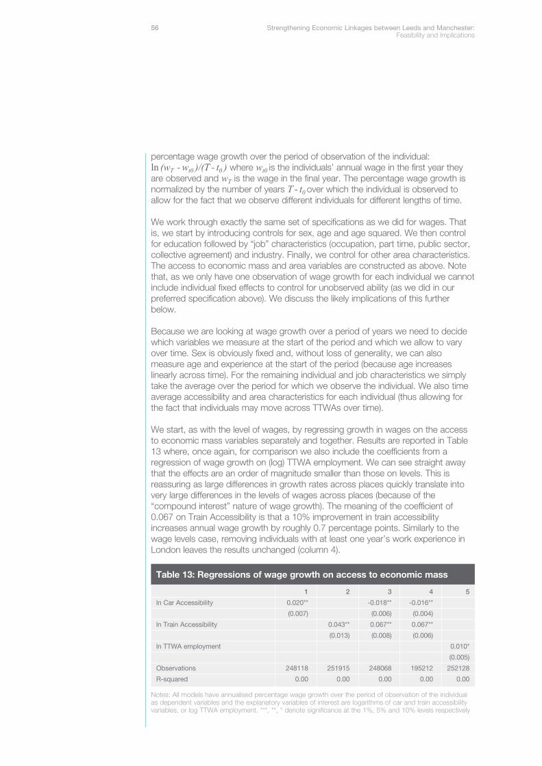
North West Development Agency:Damian Bourke, Nidi Etim
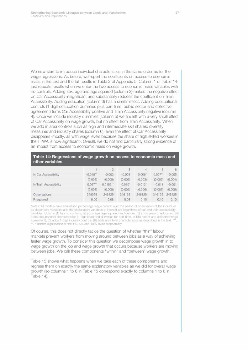
The Northern Way:Andrew Lewis, John Jarvis, Richard Baker
Yorkshire Forward: Nicky Denison, Simon Foy, Andrew Lowson
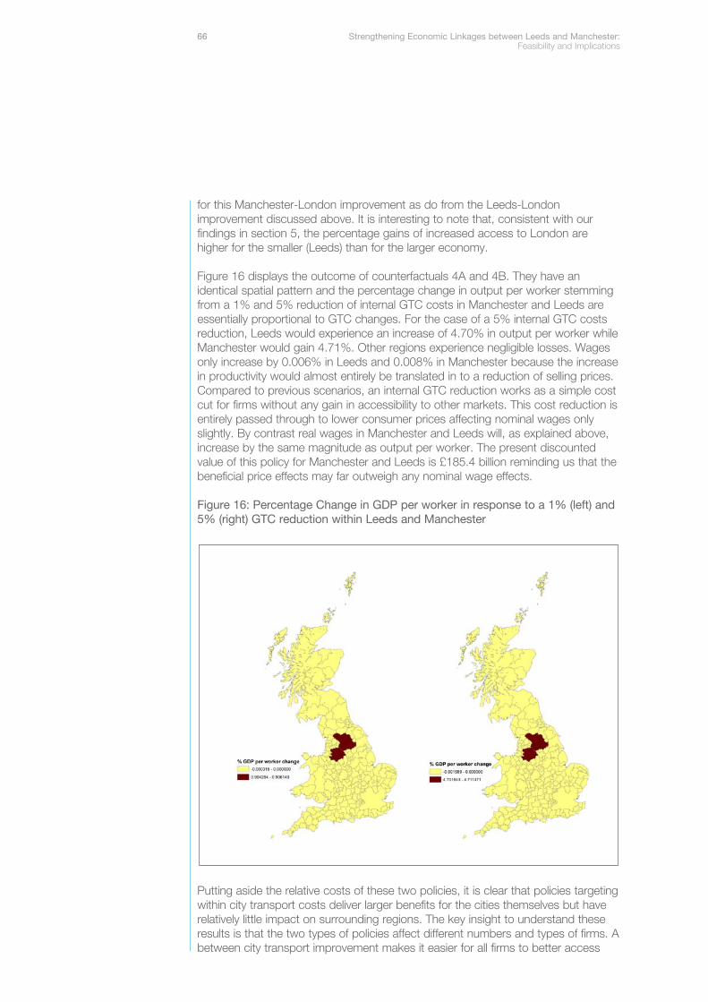
Independent Academic Advisor: Professor Alan Harding, IPEG, University of Manchester
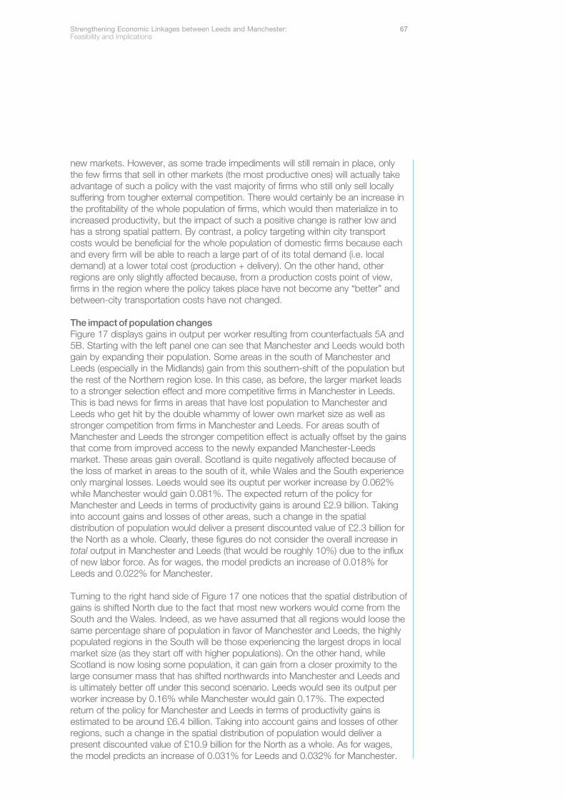
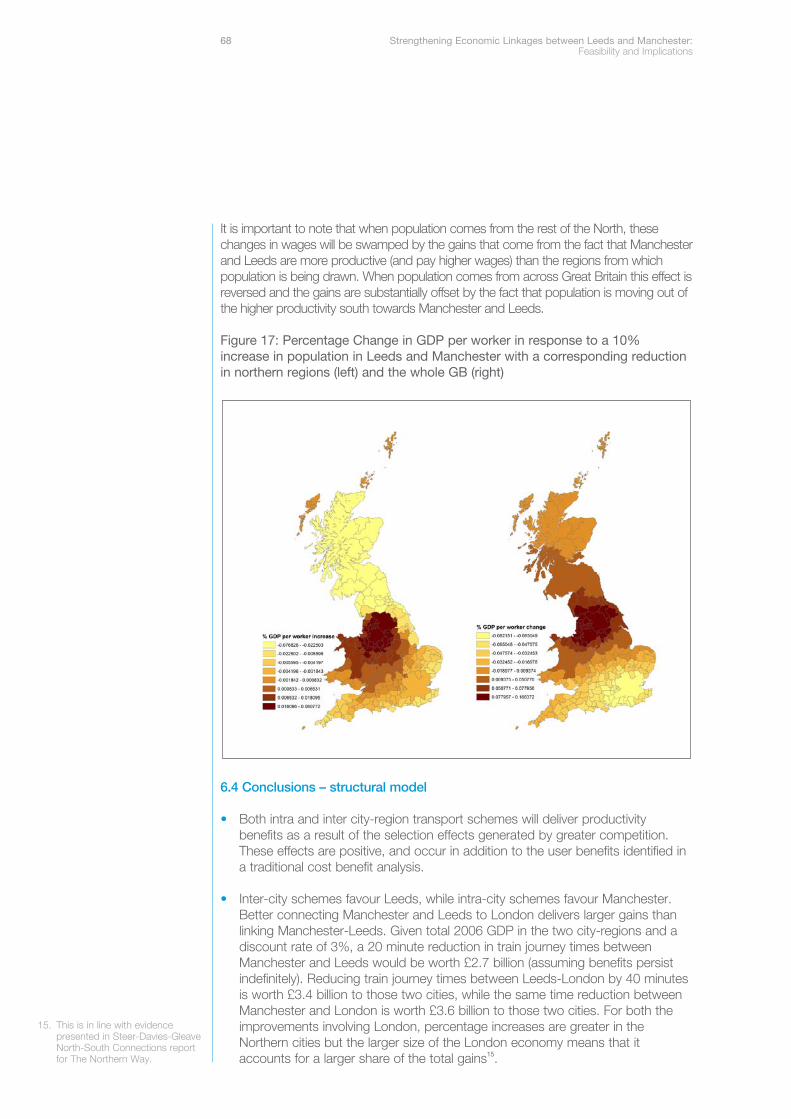
Strengthening Economic Linkages between Leeds and Manchester: 1Feasibility and Implications
1. Introduction 2
2. Background to research 3
3. Commuting flows 63.1 Gravity Model 63.2 Data Sources 73.3 Results 83.4 Conclusions 12
4. Interactions in earnings, employment and output 164.1 Data Description 164.2 Exploratory spatial data analysis 194.2.1 Moran’s I statistics 234.2.2 Spatial Weight Matrix (W) 234.2.3 ESDA Results 244.3 Spatial Econometric Analysis 334.4 Conclusions – Spatial Econometric Analysis 41
5. Agglomeration and labour markets 425.1 Methodology and Data 435.2 Results 455.3 The labour market impacts of closer integration 525.4 Results: wage growth 555.5 Labour markets and agglomeration: conclusions 60
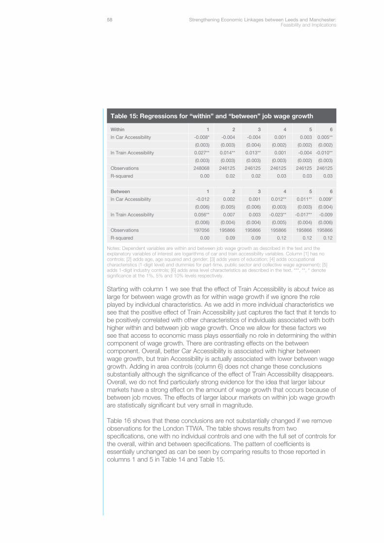
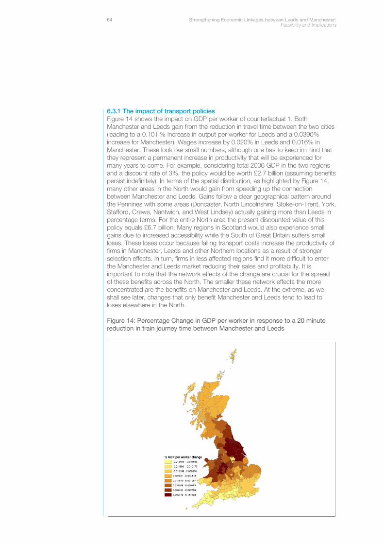
6. A structural model to examine the impacts of policy 616.1 An Introduction to Heterogeneous Firm Models 626.2 Data 636.3 Counterfactuals 636.3.1 The impact of transport policies 64
The impact of population changes 676.4 Conclusions – structural model 68
7. Overall conclusions 70
8. References 72
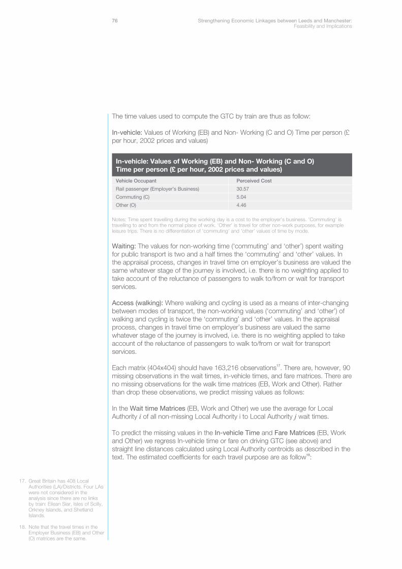
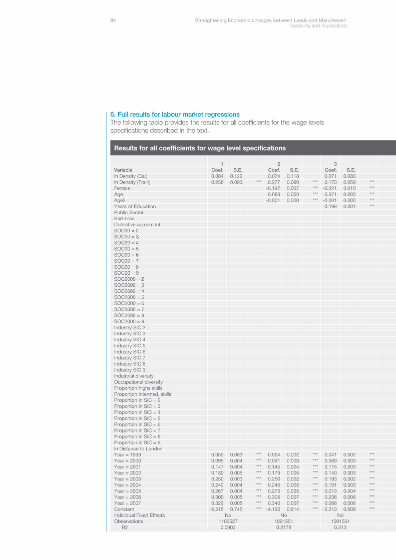
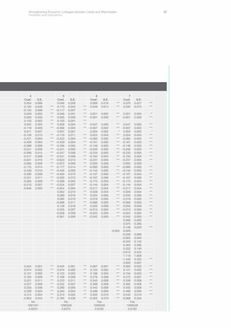
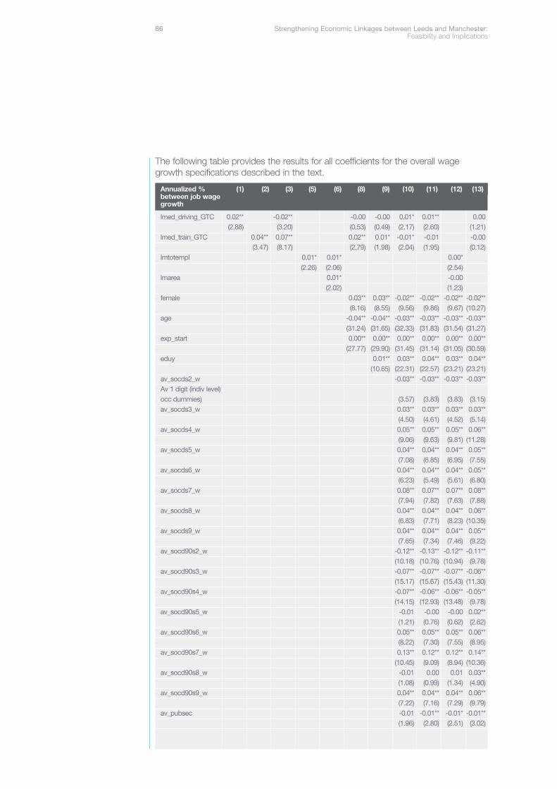
Appendices 741 The ASHE and NES databases 742 Generalised Transport Costs and Counterfactuals 752.1 Generalised Transport Costs (GTCs) 752.2 Conterfactuals 783 Definitions of city regions 784 Data for spatial econometrics & structural model 805 Additional results for spatial econometrics section 826 Full results for labour market regressions 84
Contents
2 Strengthening Economic Linkages between Leeds and Manchester: Feasibility and Implications
This report describes research by the Spatial Economics Research Centre that aimsto understand economic integration and interaction between the Manchester andLeeds city-regions. As well as analyzing current patterns, the research assesses thepossible economic impacts of increased integration.
The research was commissioned by The Northern Way, as a contribution to itsPolicy and Research programme, to provide robust evidence about the economicrelationships between the two city-regions and to assess:
• economic opportunities which could accrue from closer links; to the two city-regions, other Northern territories and the wider UK
• risks, either in terms of adverse impacts on the economy of one of the twocentres, or impacts on surrounding territories
• the potential and feasibility for public policy to stimulate and encourage suchrelationships.
The research involved a number of complementary projects, and it was undertakenbetween July 2008 and November 2009. Facilitated by The Northern Way, theproject was supported by representatives from the two city-regions, YorkshireForward and the North West Development Agency, Government Departments andindependent academic advisors.
This report, describes the detailed findings and methodology. Alongside a summaryof findings and policy conclusions, it is available on the website of The NorthernWay at www.thenorthernway.co.uk/leedsmanchester and SERC atwww.spatialeconomics.ac.uk.
1. Introduction
Strengthening Economic Linkages between Leeds and Manchester: 3Feasibility and Implications
There is increasing interest in the role of cities in driving economic growth anddevelopment
An immediate focus is on the role cities may play in recovery from the currentrecession. However, beyond this the importance of cities to the economy and thusto economic policy is increasingly recognized at both national and internationallevels. In the UK, this increased interest reflects the fact that, after a long period ofrelative decline, a significant number of English cities have experienced improvedeconomic performance (ODPM, 2006). At the same time, evidence about underlyingstructural changes, suggests there may be potential for continued long term growthin these cities.
In particular, if the UK economy continues its inexorable move from manufacturingto services, this will have important implications for continued growth in cities. Thereis a large body of evidence which suggests that producers of services benefit in avariety of ways when they locate in cities. Crucially, the benefits of thisagglomeration appear to be larger for service producers than for manufacturers. Astructural shift towards services, combined with the fact that services benefit morefrom cities, points towards a future in which more economic activity could beconcentrated in a small number of larger cities.
Amongst policy makers in the UK, particularly those concerned with spatialdisparities, this raises a number of important questions. Will this growth beconcentrated mostly in London and the Greater South East? If so, is there anythingthat policy can, or should, do to counteract this? What role might future growth inNorthern cities play in increasing growth in the wider northern economy? Whichcities in the North might drive this growth and what, if anything, might be theappropriate role for policy? The research that we describe in this report isconcerned with the last of these questions. In particular, we consider theimplications and feasibility of developing stronger economic relationships betweenthe Manchester and Leeds city-regions.
Recent reports for The Northern Way from IPEG/CUPS1 and the Centre for Cities2
have assembled extensive evidence describing the economic connections betweenNorthern cities and between the Northern cities and London. This research hasserved to reinforce the longstanding sense within The Northern Way, and thoseworking around it, that one of the key opportunities for the acceleration of growthavailable to the north of England as a whole may be the stimulation of higher levelsof integration between the Manchester and Leeds economies. These cities are ofparticular interest because, while both cities have recently experienced stronggrowth, existing research finds little evidence of interaction in terms of businessconnections or commuting, despite their geographical proximity. Our researchbuilds on this work to provide further evidence on the feasibility and implications ofstrengthening economic linkages between the Leeds and Manchester City Regions.
The fact that there is little evidence of interaction between Leeds and Manchesterhas led some commentators to conclude that the links between the two cities aresomehow weaker than they should be and that increasing these links could play apart in improving economic performance of the Northern regions. In part, thisconclusion is based on a comparison to the higher levels of interaction in otherparts of the UK, in particular in London and the South East. In part it is based oninternational comparisons, where we observe stronger economic interactions
1. See ‘The Northern Connection’.IPEG/CUPS for The NorthernWay, January 2008.
2. See ‘City Links’, Lucci & Hildreth,March 2008.
2. Background to the research
between similarly sized cities positioned close to each other. Commentators havesought to explain these weak links as arising from a number of factors including;topography (in particular the Pennines), cultural differences and poor transportconnections.
In developing this research, we recognized that an analytical jump from theobservation of low levels of interaction to the conclusion that integration is weakerthan it should be is not warranted. Further evidence on the links between the twoeconomies is needed to help assess the case for intervention and to understandwhether increasing integration has any role to play in improving the economicperformance of the two city regions or the wider northern economy.
To reach the conclusion that integration is weaker than expected, one needs to beable to make a comparison to an appropriate benchmark. Arguably, neither Londonand the Greater South East, nor a limited number of international cities provideparticularly compelling comparators. Therefore, in the first stage of our analysis werevisit this issue and use regression analysis to construct more appropriatebenchmarks based on observed behaviour across the whole of Great Britain. Westart by considering commuting – the only “flow” between places in Great Britain forwhich we have reasonable data. We ask what determines commuting flowsbetween places and, given this, whether flows between Manchester and Leeds areactually lower than expected. We then turn our attention to outcomes that are ofgreater policy interest, namely earnings, employment and output. Here, unlike withcommuting, we are unable to directly observe the interactions between places.Instead, we consider the extent to which nearby places appear to experience similarlevels of, and changes in, these outcomes. Again, we use observed behaviouracross the whole of Great Britain to ask what determines these similarities andwhether Manchester and Leeds are in any sense unusual.
Both these approaches essentially divide outcomes in to a part that can beexplained by things that are observed about places and a residual, or unobserved,part. This distinction is of more than academic interest. If policy makers want toincrease interaction between the Manchester and Leeds economies, then theappropriate policy response will depend crucially on what causes the degree ofinteraction to be low in the first place. Addressing cultural differences requires adifferent set of policies to those needed to address high travel costs. Knowing whathelps explain the behaviour we observe is a good starting point for thinking aboutpolicy. It is in this sense – of trying to understand observed behaviour – that weconsider questions of the “feasibility” of increasing integration between Manchesterand Leeds. In the second part of the study we turn to the implications of doing sowith a particular focus on the effect on economic performance in the north.
We approach this question of the implications for economic performance in twoways. The first is to view enhanced integration between Manchester and Leeds as away of increasing the size of the local economy. A larger local economy may helpfirms be more productive. Such agglomeration economies – as economists refer tothe beneficial effects of a larger local economy – may arise for a variety of reasons.In particular large local economies may facilitate sharing of resources (for example oflarge infrastructure such as airports), matching of capacity (for example of the rightworkers to the right firms) or learning (for example a transfer of knowledge from onefirm to another). Can we say anything about the likely impact of these effects if weachieved increased integration between Manchester and Leeds? Existing work forThe Northern Way has tackled this question by using estimates of the strength of
4 Strengthening Economic Linkages between Leeds and Manchester: Feasibility and Implications
agglomeration economies, coupled with assumptions on the extent to whichintegration would increase local economy size to work out the productivity impactson different sectors of the economy. We use labour market data to try tounderstand whether this existing work captures all the likely impacts of increasedintegration.
There has been considerable speculation that the size of the Manchester and Leedseconomies may have negative implications for labour market outcomes and thatthis may be an important factor in explaining their relative under performance. Toexamine this possibility we use data on individual wages to see how the level andgrowth of wages are affected by the size of the local labour market. We then assessthe extent to which these benefits arise from changing composition (e.g. large citieshave more educated workers) as opposed to higher wages for existing workers. Wethen use our estimates, coupled with realistic assumptions about policy inducedchanges in transport costs, to assess the impact of increased integration on labourmarket outcomes.
Our work on labour markets views enhanced integration between Manchester andLeeds as a way of increasing the size of the local economy and studies the impacton the structure of the economy and on wages. The method that we use, referredto as a “reduced form” approach, makes it hard to be specific about the economicchannels through which these effects operate. This, in turn, means we cannot sayanything precise about how these effects will impact on the wider Northerneconomy. In the final part of our research we examine these impacts using whateconomists refer to as a “structural model”. This model is very specific about thechannels through which increased integration impacts productivity. We focus, inparticular, on selection effects that are thought to generate a large part of theproductivity increase that we observe as economies become more integrated. Thestrength of these selection effects depends on both the size of the local economyand the extent of integration with other local economies. This means that we canuse the model, fitted to GB data, to examine how increased integration affectsproductivity across different economies and so get some idea of how closerManchester-Leeds integration might affect other places in the North.
The rest of this report is structured as follows. Section 3 considers commutingflows. Section 4 considers linkages in output and employment. Section 5 considersthe role of labour markets, while Section 6 outlines the findings from our structuralmodel. Section 7 provides conclusions and considers policy issues.
Strengthening Economic Linkages between Leeds and Manchester: 5Feasibility and Implications
We are interested in understanding the determinants of commuting betweenManchester and Leeds. We focus on commuting flows because (i) they are likely tobe a very important driver of linkages between places; (ii) unlike, say, businessinput-output linkages, we have sufficiently detailed data to undertake analysis of thedeterminants. We have undertaken analysis to try to answer two related questions.First, given the overall level of commuting flows in and out of Manchester andLeeds, are the bilateral flows between Manchester and Leeds unusually high orlow? Second, to what extent do characteristics of Manchester and Leeds (that is,characteristics that we can observe in the data – size, income, commuting costs)explain these patterns? To answer these questions we model data on commutingflows between Local Authority areas across Great Britain as a function of thecharacteristics (size, income, commuting costs) of those Local Authority areas. Wethen compare outcomes for Manchester and Leeds to those that we would predictbased on their characteristics and the observed behaviour of commuters acrossGreat Britain.
3.1 Gravity ModelWe use a version of the ‘gravity’ model to explain commuting flows between places.In its most basic form, the model assumes that the degree of interaction betweenplaces depends positively on their “mass” – e.g. an area’s population oremployment – and negatively on the distance between places.
The gravity model has been widely used in the social sciences to study spatialinteraction. In particular, it has been extensively used to examine trade betweencountries. See Overman, Redding and Venables (2003) and Anderson and vanWincoop (2004) for surveys.
Papers on commuting behaviour have also employed the gravity model, typically tostudy commutes within a single metropolitan area. Examples include studies ofWashington D.C. by Levinson (1998) and the San Francisco Bay Area by Cerveroand Wu (1997). Applications of the gravity model to commuting behaviour in the UKare scarce, though Coombes and Raybould (2001) investigate the regionalcharacteristics associated with short commutes (less than 5km) in England andWales.
In this project we use the gravity model to investigate commute patterns betweenLocal Authority areas across the whole of Great Britain. The gravity model to explainthe number of home-to-work commutes between any two areas can be expressedformally as:
Tij =AiBj exp[-θcij]
where Tij denotes the number of commutes between i and j, Ai is an originfunction, Bj a destination function and cij is a deterrence function3. The originfunction captures anything specific to the origin (i.e. the point from which acommute starts) that might affect overall commuting flows to all destinations. Thedestination function does similarly for all destinations (i.e. the point at which acommute ends). The deterrence function captures the factors, such as distance,that might inhibit flows between locations i and j. We use an exponential deterrencefunction which is popular in the literature because it leads to a gravity model with anumber of desirable properties. See Sen and Smith (1995) for further discussion. 3. Given that our focus is on
commuting between Manchesterand Leeds we ignore within LocalAuthority commuting flows.
3. Commuting flows
6 Strengthening Economic Linkages between Leeds and Manchester: Feasibility and Implications
Taking logs of both sides of the equation gives:
ln (Tij ) = ln (Ai) + ln (Bj) -θcij
This is the version of the gravity equation that forms the basis for our empiricalwork.
In terms of the origin and destination characteristics, we model the number ofcommutes between two Local Authority areas i and j as driven by (i) the size of theLocal Authority areas as measured by employment and (ii) the average wages ineach Local Authority area. We also assume that, even allowing for these factors,some Local Authority areas will have high inward commutes (e.g. city centres) somehigh outward commutes (e.g. residential areas). Rather than trying to identify all thedifferent factors that might cause areas to have high outflows or inflows in a givenyear, we just capture the effect in the model by including dummy (zero-one)variables that indicate a given origin or destination Local Authority area. Thesedummy variables allow the data to tell us when commutes are unusually high or lowfor a specific Local Authority area. We start by using straight line distances betweenareas as the factor that deters commutes. We then turn to more realistic measuresof transport costs by road and train.
Technically, it is not possible to estimate the parameters on observable factors thatare area specific (e.g. employment) -and at the same time control for area effects.Therefore, to demonstrate the effect of origin and destination characteristics weimplement the gravity equation in three steps. We first estimate the model in termsof the influence of destination characteristics allowing for unexplained differences inthe flows out of different origins using origin dummy variables. We then estimate themodel in terms of the influence of origin characteristics allowing for unexplaineddifferences in terms of the attractiveness of different destinations using destinationdummy variables. Finally we combine the two estimates to calculate the residual orunexplained part of the commuting flows4. We base our final conclusions, however,on the more general model which allows origin and destination dummies to captureeverything specific to origins and destinations allowing us to focus on the role oftransport costs in deterring commuting.
We expect that distance and transport costs should have a negative effect oncommutes. Wages and employment levels in the work area should have positiveeffects. In contrast, wages in the home area should have a negative effect. Homearea employment may be positive (an overall size effect) or negative (people worklocally). On average, we would expect the size effect to dominate and for thecoefficient on home employment to be positive. Beyond these explanatory variables,as we just discussed, the fixed effects capture an area’s overall tendency to be ahome- or work-commute destination.
To reiterate, this model allows us to compare the number of commutes betweenManchester and Leeds with commute patterns in the remainder of Great Britain andwith other city pairs of interest. We can then use our understanding of how thesedeterminants work on average across Great Britain to look at the specific factorsthat affect commuting between Manchester and Leeds.
3.2 Data SourcesTo implement this methodology we need data on commuting, wages, employment,distances and transport costs between locations. An easily available source of
4. We estimate the residual as rij = ln (Tij ) − [ln(T̂ij
o) + ln(T̂ij
d)]/2]
where a hat over the T indicatesthat it is predicted from the origin(superscript o) or destination(superscript d) regressions.
Strengthening Economic Linkages between Leeds and Manchester: 7Feasibility and Implications
commuting data is the 2001 Census which is appealing as it is based on the entirepopulation. However, this data is relatively old and so we instead use the AnnualSurvey of Hours and Earnings (ASHE) dataset. ASHE is constructed by the Officeof National Statistics (ONS) based on a 1% sample of employees on the InlandRevenue PAYE register for February and April. It provides specific information onindividuals including their home and work postcodes. The National StatisticsPostcode Directory (NSPD) provides a mapping from every UK postcode tohigher-level geographic units (e.g. output area, government office region, country,etc). Merging this data with each ASHE-individual’s home and work postcode weare able to calculate the number of people commuting from one Local Authorityarea to another. We use these as our estimates of annual work-commute patternsacross Great Britain for the years 2002-20055. To increase the underlying samplesize and to mitigate the problem that time series variation in this data can be drivenby year-to-year variations in the sample we simply average across years and try toexplain the average flows between 2002 and 2005 as a function of similarly timeaveraged area characteristics.
ASHE also includes information on occupation codes, industry code, private/publicsector, age, gender and detailed information on earnings including base pay,overtime pay, basic and overtime hours worked. We use information on basic hourlyearnings to calculate average wages by Local Authority area. This raises someconcerns about local sample sizes from ASHE. Investigation suggests that this maybe an issue for some rural LA, but not for primary urban areas. ASHE does notprovide years of education so we construct these using cohort of birth-by-SOCmatching on data from the LFS which contains information on both occupationsand education. The way that we do that is described in Appendix 1 which alsoprovides further details on the ASHE database.
To estimate employment in each area we use the Business Structure Databasewhich provides an annual snapshot of the Inter-Departmental Business Register(IDBR). This dataset contains information on 2.1 million businesses, accounting forapproximately 99% of economic activity in the UK and includes each business’name, postcode, industry code, number of employees, total employment (includingowners), legal status and country of ownership6. From each firm’s business addressand total employment, we calculate the total employment in each Local Authorityarea.
We identify the centre of Local Authority areas using information on postcodelocations and calculate distances as the straight line distance between thesecentroids. Coordinates (northing and easting) for all UK postcodes are provided bythe NSPD. From these, we define an area’s centroid as the average across all of itspostcode coordinates. Since the number of postcodes increases roughly inproportion to population, this calculation of an area’s centroid gives a roughestimate of the area’s center-of-gravity by population. The distance between thecentroids is then calculated using the Pythagorean Theorem. We constructGeneralized Transport Costs (GTC) for train and driving as detailed in Appendix 2.
3.3 ResultsAs explained above we initially estimate two separate models. The first explainscommuting as a function of destination characteristics allowing for unobservedcharacteristics of origins to affect commuting. The second explains commuting as afunction of origin characteristics, allowing unobserved characteristics of destinationsto affect commuting. For both origins and destinations we start with a very simple
5. Dan Graham (from ImperialCollege, London) has beenworking for DfT to assess whetherthe sample contained in ASHE issufficiently representative to allowreasonable estimation ofcommuting flows (by comparingto the 2001 census). The resultsof this work are not yet published,but in private correspondence hehas confirmed that ASHE basedestimates of commuting flowsshould be sufficiently accurate forthe kind of modeling exercise thatwe wish to undertake.
6. The 99% coverage was lastverified in 2004/05, although thereis no reason to think that this isnot still the case.
8 Strengthening Economic Linkages between Leeds and Manchester: Feasibility and Implications
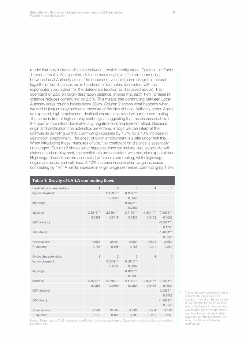
model that only includes distance between Local Authority areas. Column 1 of Table1 reports results. As expected, distance has a negative effect on commutingbetween Local Authority areas. The dependent variable (commuting) is in naturallogarithms, but distances are in hundreds of kilometres (consistent with theexponential specification for the deterrence function as discussed above). Thecoefficient of 2.53 on origin-destination distance, implies that each 1km increase indistance reduces commuting by 2.5%. This means that commuting between LocalAuthority areas roughly halves every 30km. Column 2 shows what happens whenwe add in (log) employment as a measure of the size of Local Authority areas. Again,as expected, high employment destinations are associated with more commuting.The same is true of high employment origins suggesting that, as discussed above,the positive size effect dominates any negative local employment effect. Becauseorigin and destination characteristics are entered in logs we can interpret thecoefficients as telling us that commuting increases by 1.7% for a 10% increase indestination employment. The effect of origin employment is a little under half this.When introducing these measures of size, the coefficient on distance is essentiallyunchanged. Column 3 shows what happens when we include (log) wages. As withdistance and employment, the coefficients are consistent with our prior expectations.High wage destinations are associated with more commuting, while high wageorigins are associated with less. A 10% increase in destination wage increasescommuting by 1%7. A similar increase in origin wage decreases commuting by 1.8%.
7. This is the only coefficient that issensitive to the inclusion ofLondon. If we drop the one thirdof our sample for which at leastone of the LAs is in the LondonCity Region we no longer find asignificant effect of destinationwage on commuting flows. Ourother results are otherwiseunaffected.
Strengthening Economic Linkages between Leeds and Manchester: 9Feasibility and Implications
Notes: Table reports OLS regression coefficients and standard errors. Dependent variable is log commuting.Source: ONS
Columns 1 to 3 separately model the effects of destination characteristics allowingfor unobserved origin effects and origin characteristics allowing for unobserveddestination effects. Column 4 shows the combined model where we allow for bothunobserved origin and destination characteristics to drive commuting. As explainedabove, we can no longer separately identify the affect of observable origin anddestination characteristics. We can, however, still identify the effect of distance oncommuting flows (because this is origin-destination) specific. As is clear fromcolumn 4 the effect of distance is largely unchanged. Note also, that once weinclude both origin and destination fixed effects the origin and destinationspecifications are identical so we get the same results for both. Finally, column 5shows what happens when we introduce measures of generalized transport costs(GTC) that capture both the monetary and time costs of travel. The effect of bothtrain and driving GTC is negative while the impact of straight line distance is nowpositive. GTC are measured in £100’s of pounds so the coefficients tell us that a£100 increase in GTC reduces commuting by 3.1% for driving, 1.4% for train.These effects are not particularly large (possibly because GTC’s tend to respondpositively to commuting flows). The positive coefficient on distance tells us that,once we condition on transport costs, distances are actually associated with morecommuting (although the effect is small in magnitude). This is clearly not a causallinkage. A likely theoretical explanation for this finding is that longer commutesbetween cities with better (and therefore lower cost) transport links are moreprevalent than other types of shorter LA-LA commute that involve similar transportcosts. In practice, the distance and driving GTC variables are very highly correlatedwith each other, which makes it difficult to disentangle their separate effects oncommuting8. One final thing to note, before turning to the specific question of thelinks between Manchester and Leeds is that the models are ranked in order of theirability to explain the overall variation in commuting (note that the R-square increasesas we move across the columns).
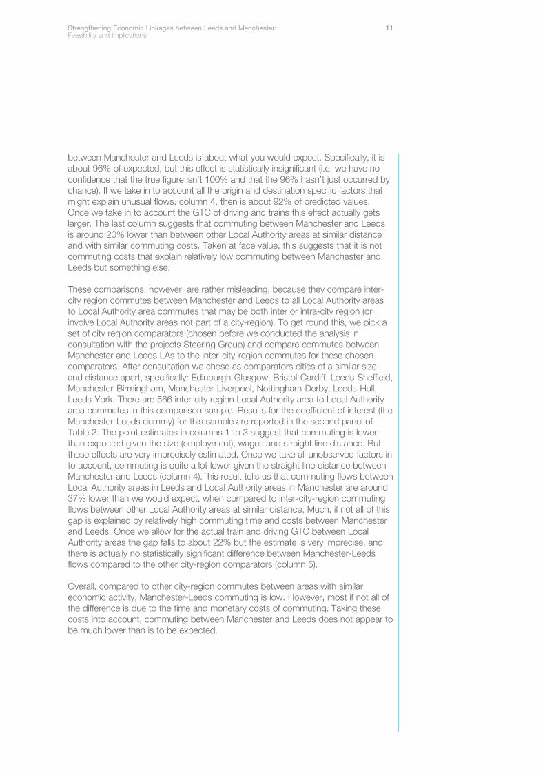
As explained above, we can now use these gravity models to see whethercommuting between Manchester and Leeds is higher or lower than expected. Wedo this by comparing predicted commuting between Local Authority areas inManchester and Leeds with actual commuting. There are 15 Local Authorities in theManchester City Region and 8 Local Authorities in the Leeds City-Region (Appendix3 describes how we construct these city regions). Thus we need to compare the120 bilateral flows between Manchester and Leeds to the 35,428 other LocalAuthority pairs that have positive commuting flows for which we are able tocompare predicted to actual commuting. We use a simple regression analysis tomake this comparison. Specifically, we regress the Local Authority area to LocalAuthority area residual log commuting flows on dummy variables that indicatewhether these flows are to or from Manchester, to or from Leeds, or betweenLeeds and Manchester (in either direction). The top panel of Table 2 shows theresults when running regressions on all Local Authority area to Local Authority areapairs. Each column 1 to 5 corresponds to the five specifications that we describedabove (the results of which are reported in columns 1 to 5 of Table 1).
Looking across the columns in the top panel it is evident that both Manchester andLeeds Local Authority areas have lower mean inflows and outflows than we wouldexpect given their employment, wages and geographical position relative to otherLocal Authority areas. Even given these relatively low flows in and out ofManchester, commuting between Manchester and Leeds Local Authority areas islower than expected, but the pattern of coefficients is not simple. If we just modelcommuting as driven by size (employment), wages and distance, commuting
8. We have tried alternativespecifications using additionalterms in the square of distanceand transport costs, including theproduct of employment and theratio of wages (to allow for morecomplex interactions). None ofthese changes alter the overallpattern of coefficients or ourconclusions based on analysis ofthe residuals from these morecomplex specifications.
10 Strengthening Economic Linkages between Leeds and Manchester: Feasibility and Implications
between Manchester and Leeds is about what you would expect. Specifically, it isabout 96% of expected, but this effect is statistically insignificant (i.e. we have noconfidence that the true figure isn’t 100% and that the 96% hasn’t just occurred bychance). If we take in to account all the origin and destination specific factors thatmight explain unusual flows, column 4, then is about 92% of predicted values.Once we take in to account the GTC of driving and trains this effect actually getslarger. The last column suggests that commuting between Manchester and Leedsis around 20% lower than between other Local Authority areas at similar distanceand with similar commuting costs. Taken at face value, this suggests that it is notcommuting costs that explain relatively low commuting between Manchester andLeeds but something else.
These comparisons, however, are rather misleading, because they compare inter-city region commutes between Manchester and Leeds to all Local Authority areasto Local Authority area commutes that may be both inter or intra-city region (orinvolve Local Authority areas not part of a city-region). To get round this, we pick aset of city region comparators (chosen before we conducted the analysis inconsultation with the projects Steering Group) and compare commutes betweenManchester and Leeds LAs to the inter-city-region commutes for these chosencomparators. After consultation we chose as comparators cities of a similar sizeand distance apart, specifically: Edinburgh-Glasgow, Bristol-Cardiff, Leeds-Sheffield,Manchester-Birmingham, Manchester-Liverpool, Nottingham-Derby, Leeds-Hull,Leeds-York. There are 566 inter-city region Local Authority area to Local Authorityarea commutes in this comparison sample. Results for the coefficient of interest (theManchester-Leeds dummy) for this sample are reported in the second panel ofTable 2. The point estimates in columns 1 to 3 suggest that commuting is lowerthan expected given the size (employment), wages and straight line distance. Butthese effects are very imprecisely estimated. Once we take all unobserved factors into account, commuting is quite a lot lower given the straight line distance betweenManchester and Leeds (column 4).This result tells us that commuting flows betweenLocal Authority areas in Leeds and Local Authority areas in Manchester are around37% lower than we would expect, when compared to inter-city-region commutingflows between other Local Authority areas at similar distance, Much, if not all of thisgap is explained by relatively high commuting time and costs between Manchesterand Leeds. Once we allow for the actual train and driving GTC between LocalAuthority areas the gap falls to about 22% but the estimate is very imprecise, andthere is actually no statistically significant difference between Manchester-Leedsflows compared to the other city-region comparators (column 5).
Overall, compared to other city-region commutes between areas with similareconomic activity, Manchester-Leeds commuting is low. However, most if not all ofthe difference is due to the time and monetary costs of commuting. Taking thesecosts into account, commuting between Manchester and Leeds does not appear tobe much lower than is to be expected.
Strengthening Economic Linkages between Leeds and Manchester: 11Feasibility and Implications
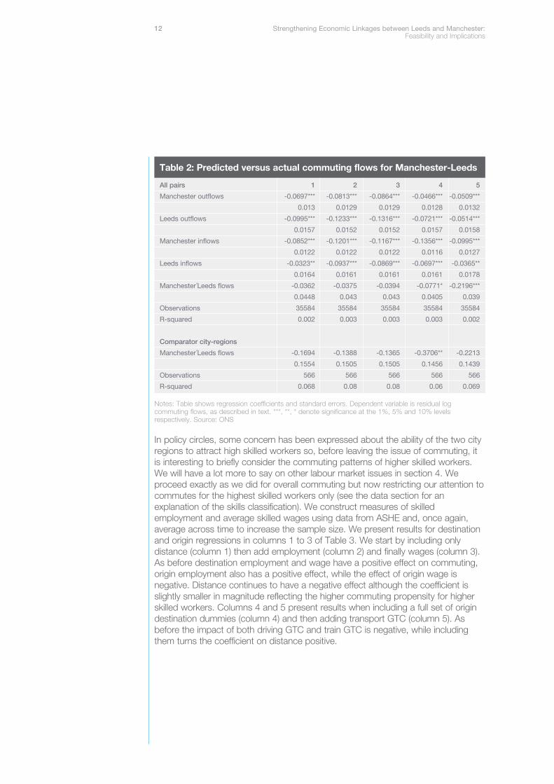
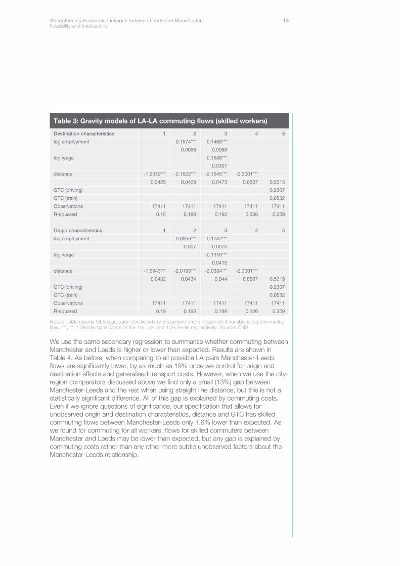
In policy circles, some concern has been expressed about the ability of the two cityregions to attract high skilled workers so, before leaving the issue of commuting, itis interesting to briefly consider the commuting patterns of higher skilled workers.We will have a lot more to say on other labour market issues in section 4. Weproceed exactly as we did for overall commuting but now restricting our attention tocommutes for the highest skilled workers only (see the data section for anexplanation of the skills classification). We construct measures of skilledemployment and average skilled wages using data from ASHE and, once again,average across time to increase the sample size. We present results for destinationand origin regressions in columns 1 to 3 of Table 3. We start by including onlydistance (column 1) then add employment (column 2) and finally wages (column 3).As before destination employment and wage have a positive effect on commuting,origin employment also has a positive effect, while the effect of origin wage isnegative. Distance continues to have a negative effect although the coefficient isslightly smaller in magnitude reflecting the higher commuting propensity for higherskilled workers. Columns 4 and 5 present results when including a full set of origindestination dummies (column 4) and then adding transport GTC (column 5). Asbefore the impact of both driving GTC and train GTC is negative, while includingthem turns the coefficient on distance positive.
12 Strengthening Economic Linkages between Leeds and Manchester: Feasibility and Implications
All pairs 1 2 3 4 5
Manchester outflows -0.0697*** -0.0813*** -0.0864*** -0.0466*** -0.0509***
Table 2: Predicted versus actual commuting flows for Manchester-Leeds
Notes: Table shows regression coefficients and standard errors. Dependent variable is residual logcommuting flows, as described in text. ***, **, * denote significance at the 1%, 5% and 10% levelsrespectively. Source: ONS
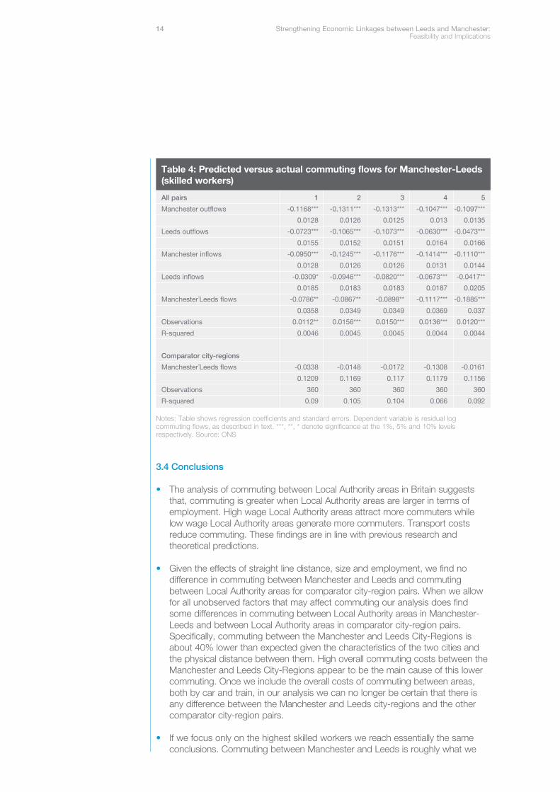
We use the same secondary regression to summarise whether commuting betweenManchester and Leeds is higher or lower than expected. Results are shown inTable 4. As before, when comparing to all possible LA pairs Manchester-Leedsflows are significantly lower, by as much as 19% once we control for origin anddestination effects and generalised transport costs. However, when we use the city-region comparators discussed above we find only a small (13%) gap betweenManchester-Leeds and the rest when using straight line distance, but this is not astatistically significant difference. All of this gap is explained by commuting costs.Even if we ignore questions of significance, our specification that allows forunobserved origin and destination characteristics, distance and GTC has skilledcommuting flows between Manchester-Leeds only 1.6% lower than expected. Aswe found for commuting for all workers, flows for skilled commuters betweenManchester and Leeds may be lower than expected, but any gap is explained bycommuting costs rather than any other more subtle unobserved factors about theManchester-Leeds relationship.
Strengthening Economic Linkages between Leeds and Manchester: 13Feasibility and Implications
Table 3: Gravity models of LA-LA commuting flows (skilled workers)
Notes: Table reports OLS regression coefficients and standard errors. Dependent variable is log commutingflow. ***, **, * denote significance at the 1%, 5% and 10% levels respectively. Source: ONS
3.4 Conclusions
• The analysis of commuting between Local Authority areas in Britain suggeststhat, commuting is greater when Local Authority areas are larger in terms ofemployment. High wage Local Authority areas attract more commuters whilelow wage Local Authority areas generate more commuters. Transport costsreduce commuting. These findings are in line with previous research andtheoretical predictions.
• Given the effects of straight line distance, size and employment, we find nodifference in commuting between Manchester and Leeds and commutingbetween Local Authority areas for comparator city-region pairs. When we allowfor all unobserved factors that may affect commuting our analysis does findsome differences in commuting between Local Authority areas in Manchester-Leeds and between Local Authority areas in comparator city-region pairs.Specifically, commuting between the Manchester and Leeds City-Regions isabout 40% lower than expected given the characteristics of the two cities andthe physical distance between them. High overall commuting costs between theManchester and Leeds City-Regions appear to be the main cause of this lowercommuting. Once we include the overall costs of commuting between areas,both by car and train, in our analysis we can no longer be certain that there isany difference between the Manchester and Leeds city-regions and the othercomparator city-region pairs.
• If we focus only on the highest skilled workers we reach essentially the sameconclusions. Commuting between Manchester and Leeds is roughly what we
14 Strengthening Economic Linkages between Leeds and Manchester: Feasibility and Implications
All pairs 1 2 3 4 5
Manchester outflows -0.1168*** -0.1311*** -0.1313*** -0.1047*** -0.1097***
Table 4: Predicted versus actual commuting flows for Manchester-Leeds(skilled workers)
Notes: Table shows regression coefficients and standard errors. Dependent variable is residual logcommuting flows, as described in text. ***, **, * denote significance at the 1%, 5% and 10% levelsrespectively. Source: ONS
would expect given the characteristics of LAs, and the distance and generalizedtransport costs of travelling between them.
• Economic factors, specifically the overall costs of commuting between the twocities, are the most important factor in explaining these relatively low commutinglevels. This suggests that lowering these costs has an important role to play inincreasing integration between the two city regions. This in turn may improve theeconomic performance of the two city-regions as we discuss further below.
• We do not examine the role of cultural or social factors directly. However, thefact that economic factors appear to explain low commuting levels leaves littleroom for cultural or social factors to play a large part in this story. This suggeststhat such factors are unlikely to act as a barrier to increased commutingbetween the two cities if transport investment lowers the overall costs ofcommuting, or if other economic factors lead to enhanced interactions.
Strengthening Economic Linkages between Leeds and Manchester: 15Feasibility and Implications
While commuting is one of the most important ways in which interactions betweencities occur, there are of course a number of others, including linkages betweencustomers and suppliers. Unfortunately, there is very little, if any data, collected onthese other linkages. There is certainly no systematic source of data collected fordifferent places in different time periods. Therefore, for these other linkages, unlikewith commuting, we are unable to directly observe the interactions between places.Instead, we have to turn our attention to the possible effects on outcomes, whichare far harder to analyse than the interactions themselves. In this section we focusdirectly on outcomes by considering the extent to which outcomes (say increases inemployment) of city-regions tend to move together. As for the work on commuting,the strategy is to identify general relationships for Great Britain and then askwhether the relationships between Manchester and Leeds are understandable inlight of these general relationships using exploratory spatial data analysis and spatialeconometrics. We outline the data first, before describing our approach andfindings.
4.1 Data DescriptionWe consider interactions in terms of earnings, employment and output per worker.This choice is governed by three considerations. First, the availability of data.Second, output per worker and wages are key outcomes that are explained by thestructural economic model that we use later in this report to consider theimplications of increased integration between Manchester and Leeds. Third, theseare some of the most important outcomes from a regional economic developmentperspective.
Our units of analysis are a mix of Local Authorities and city regions in England,Wales and Scotland. We have 242 Local Authorities and 14 city regions. The cityregions are aggregations of the remaining 161 Local Authorities into spatial unitsthat better represent functional economic regions. In Appendix 3, we discuss howthe city regions are constructed and list the districts which belong to each cityregion. Figure 1 shows the Local Authorities and 14 city regions with which we areworking.
Local Authorities data for England, Wales and Scotland come from Nomis/ASHE(Annual Survey of Hours and Earnings) and Nomis/ABI (Annual Business Inquiry).Nomis/ASHE gives us the average hourly earnings of all full-time employees basedon the location of workplace. Nomis/ABI gives us the number of employees basedon the location of the workplace. Gross Domestic Product data (at current marketprices in millions of euros) comes from Eurostat but is only provided at NUTS3 level.We estimate GDP at district level by distributing GDP according to employmentshares calculated as the Local Authority share employment in total NUTS3employment. Appendix 4 provides more detail on the data. The exploratory spatialdata analysis will examine variables in levels in 2006 (the latest data available atLocal Authority level), in differences between 1998 and 2006, and in annual growthrates between 1998 and 2006.
4. Interactions in earnings,employment and output
16 Strengthening Economic Linkages between Leeds and Manchester: Feasibility and Implications
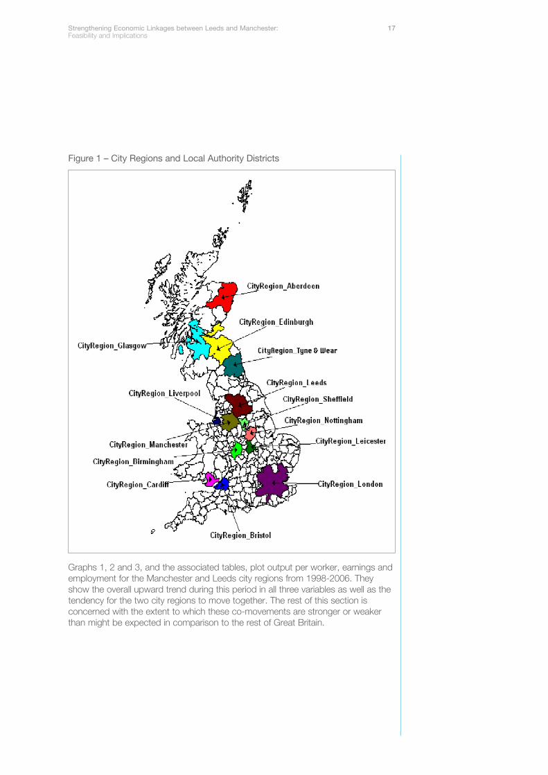
Figure 1 – City Regions and Local Authority Districts
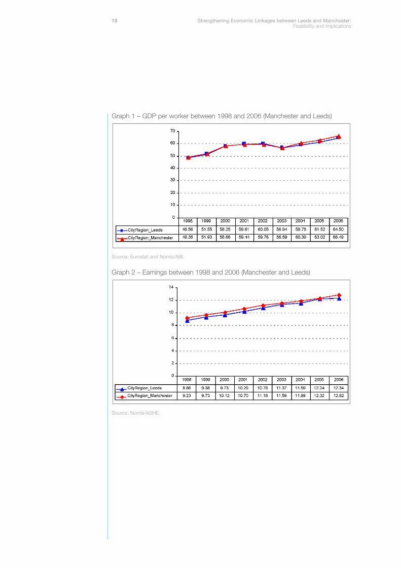
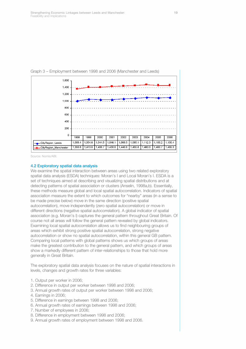
Graphs 1, 2 and 3, and the associated tables, plot output per worker, earnings andemployment for the Manchester and Leeds city regions from 1998-2006. Theyshow the overall upward trend during this period in all three variables as well as thetendency for the two city regions to move together. The rest of this section isconcerned with the extent to which these co-movements are stronger or weakerthan might be expected in comparison to the rest of Great Britain.
Strengthening Economic Linkages between Leeds and Manchester: 17Feasibility and Implications
Graph 1 – GDP per worker between 1998 and 2006 (Manchester and Leeds)
Source: Eurostat and Nomis/ABI.
Graph 2 – Earnings between 1998 and 2006 (Manchester and Leeds)
Source: Nomis/ASHE.
18 Strengthening Economic Linkages between Leeds and Manchester: Feasibility and Implications
Graph 3 – Employment between 1998 and 2006 (Manchester and Leeds)
Source: Nomis/ABI.
4.2 Exploratory spatial data analysisWe examine the spatial interaction between areas using two related exploratoryspatial data analysis (ESDA) techniques: Moran’s I and Local Moran’s I. ESDA is aset of techniques aimed at describing and visualizing spatial distributions and atdetecting patterns of spatial association or clusters (Anselin, 1998a,b). Essentially,these methods measure global and local spatial autocorrelation. Indicators of spatialassociation measure the extent to which outcomes for “nearby” areas (in a sense tobe made precise below) move in the same direction (positive spatialautocorrelation), move independently (zero spatial autocorrelation) or move indifferent directions (negative spatial autocorrelation). A global indicator of spatialassociation (e.g. Moran’s I) captures the general pattern throughout Great Britain. Ofcourse not all areas will follow the general pattern revealed by global indicators.Examining local spatial autocorrelation allows us to find neighbouring groups ofareas which exhibit strong positive spatial autocorrelation, strong negativeautocorrelation or show no spatial autocorrelation, within this general GB pattern.Comparing local patterns with global patterns shows us which groups of areasmake the greatest contribution to the general pattern, and which groups of areasshow a markedly different pattern of inter-relationships to those that hold moregenerally in Great Britain.
The exploratory spatial data analysis focuses on the nature of spatial interactions inlevels, changes and growth rates for three variables:
1. Output per worker in 2006;2. Difference in output per worker between 1998 and 2006;3. Annual growth rates of output per worker between 1998 and 2006;4. Earnings in 2006;5. Difference in earnings between 1998 and 2006;6. Annual growth rates of earnings between 1998 and 2006;7. Number of employees in 2006;8. Difference in employment between 1998 and 2006;9. Annual growth rates of employment between 1998 and 2006.
Strengthening Economic Linkages between Leeds and Manchester: 19Feasibility and Implications
20 Strengthening Economic Linkages between Leeds and Manchester: Feasibility and Implications
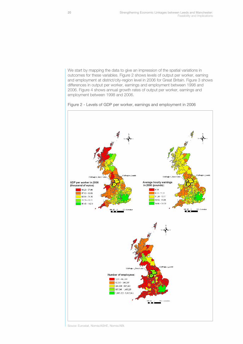
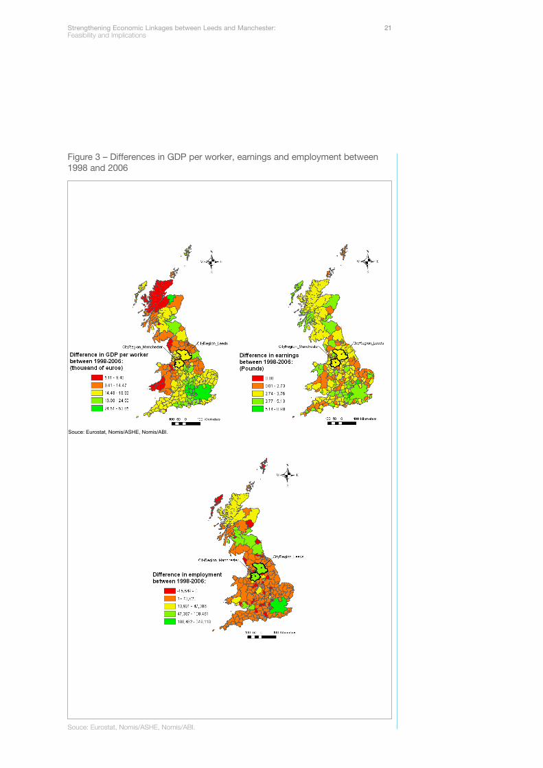
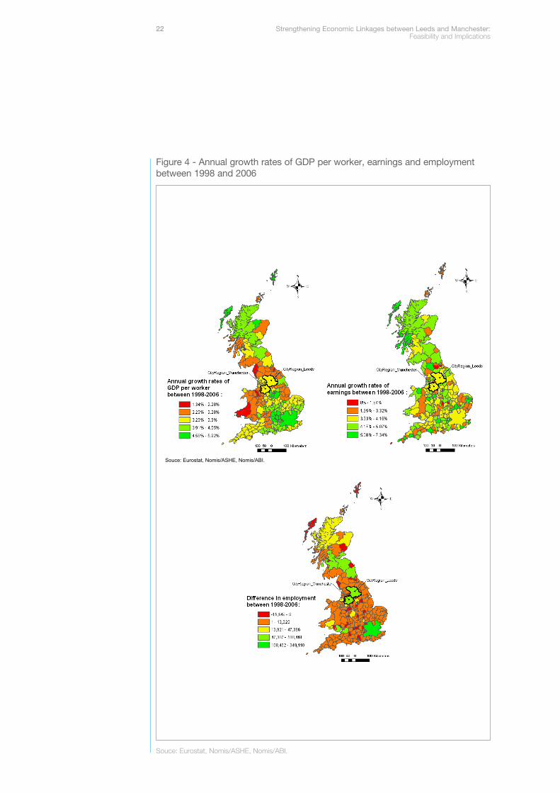
We start by mapping the data to give an impression of the spatial variations inoutcomes for these variables. Figure 2 shows levels of output per worker, earningand employment at district/city-region level in 2006 for Great Britain. Figure 3 showsdifferences in output per worker, earnings and employment between 1998 and2006. Figure 4 shows annual growth rates of output per worker, earnings andemployment between 1998 and 2006.
Figure 2 - Levels of GDP per worker, earnings and employment in 2006
Souce: Eurostat, Nomis/ASHE, Nomis/ABI.
o u c e : E u r o s t a t , N o m i s / A S H E
, N o m i s / A B I .
Figure 3 – Differences in GDP per worker, earnings and employment between1998 and 2006
Souce: Eurostat, Nomis/ASHE, Nomis/ABI.
Souce: Eurostat, Nomis/ASHE, Nomis/ABI.
Strengthening Economic Linkages between Leeds and Manchester: 21Feasibility and Implications
Figure 4 - Annual growth rates of GDP per worker, earnings and employmentbetween 1998 and 2006
Souce: Eurostat, Nomis/ASHE, Nomis/ABI.
Souce: Eurostat, Nomis/ASHE, Nomis/ABI.
22 Strengthening Economic Linkages between Leeds and Manchester: Feasibility and Implications
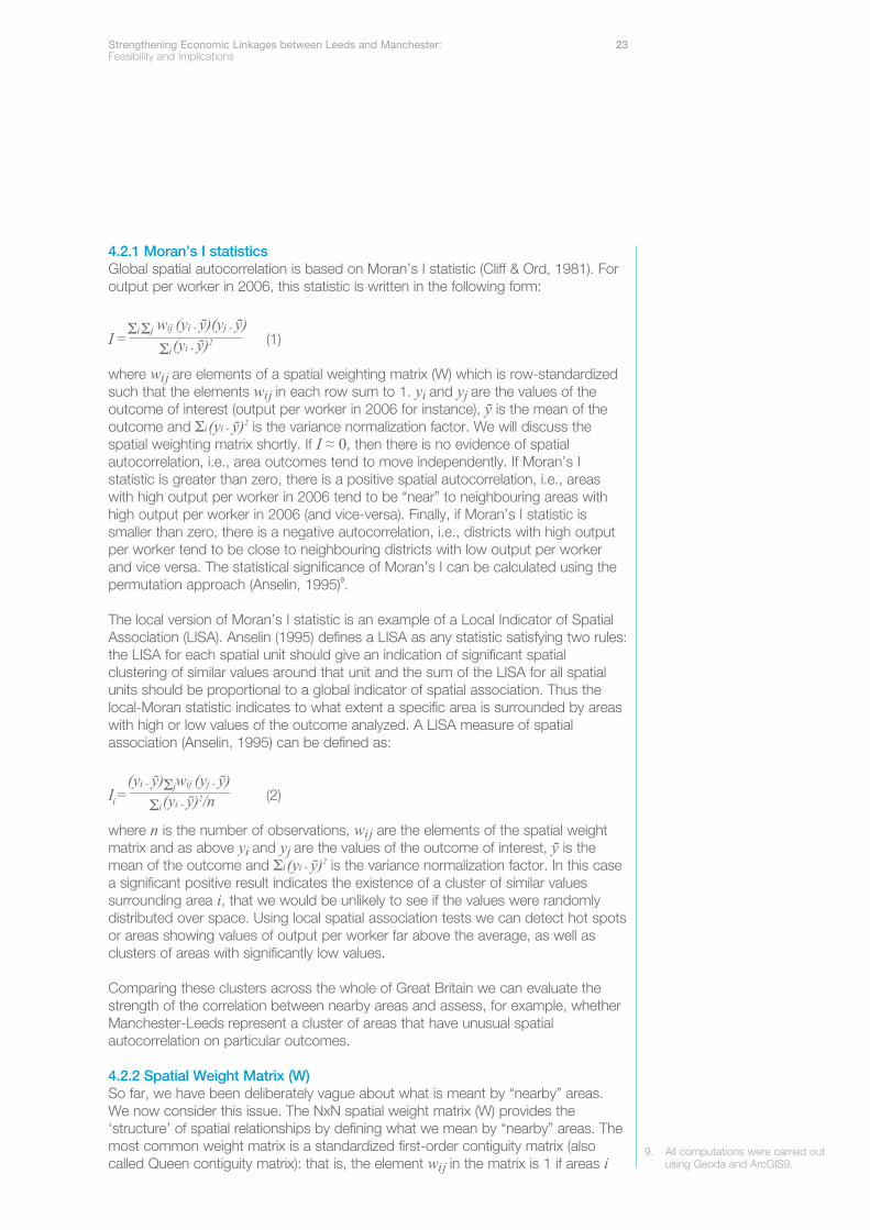
4.2.1 Moran’s I statisticsGlobal spatial autocorrelation is based on Moran’s I statistic (Cliff & Ord, 1981). Foroutput per worker in 2006, this statistic is written in the following form:
I =ΣiΣj wij (yi - ӯ)(yj - ӯ)(1)
Σi(yi - ӯ)2
where wij are elements of a spatial weighting matrix (W) which is row-standardizedsuch that the elements wij in each row sum to 1. yi and yj are the values of theoutcome of interest (output per worker in 2006 for instance), ӯ is the mean of theoutcome and Σi(yi - ӯ)2 is the variance normalization factor. We will discuss thespatial weighting matrix shortly. If I ≈ 0, then there is no evidence of spatialautocorrelation, i.e., area outcomes tend to move independently. If Moran’s Istatistic is greater than zero, there is a positive spatial autocorrelation, i.e., areaswith high output per worker in 2006 tend to be “near” to neighbouring areas withhigh output per worker in 2006 (and vice-versa). Finally, if Moran’s I statistic issmaller than zero, there is a negative autocorrelation, i.e., districts with high outputper worker tend to be close to neighbouring districts with low output per workerand vice versa. The statistical significance of Moran’s I can be calculated using thepermutation approach (Anselin, 1995)9.
The local version of Moran’s I statistic is an example of a Local Indicator of SpatialAssociation (LISA). Anselin (1995) defines a LISA as any statistic satisfying two rules:the LISA for each spatial unit should give an indication of significant spatialclustering of similar values around that unit and the sum of the LISA for all spatialunits should be proportional to a global indicator of spatial association. Thus thelocal-Moran statistic indicates to what extent a specific area is surrounded by areaswith high or low values of the outcome analyzed. A LISA measure of spatialassociation (Anselin, 1995) can be defined as:
I =(yi - ӯ)Σjwij (yj - ӯ)
(2)i Σi(yi - ӯ)2/n
where n is the number of observations, wij are the elements of the spatial weightmatrix and as above yi and yj are the values of the outcome of interest, ӯ is themean of the outcome and Σi(yi - ӯ)2 is the variance normalization factor. In this casea significant positive result indicates the existence of a cluster of similar valuessurrounding area i, that we would be unlikely to see if the values were randomlydistributed over space. Using local spatial association tests we can detect hot spotsor areas showing values of output per worker far above the average, as well asclusters of areas with significantly low values.
Comparing these clusters across the whole of Great Britain we can evaluate thestrength of the correlation between nearby areas and assess, for example, whetherManchester-Leeds represent a cluster of areas that have unusual spatialautocorrelation on particular outcomes.
4.2.2 Spatial Weight Matrix (W)So far, we have been deliberately vague about what is meant by “nearby” areas.We now consider this issue. The NxN spatial weight matrix (W) provides the‘structure’ of spatial relationships by defining what we mean by “nearby” areas. Themost common weight matrix is a standardized first-order contiguity matrix (alsocalled Queen contiguity matrix): that is, the element wij in the matrix is 1 if areas i
9. All computations were carried outusing Geoda and ArcGIS9.
Strengthening Economic Linkages between Leeds and Manchester: 23Feasibility and Implications
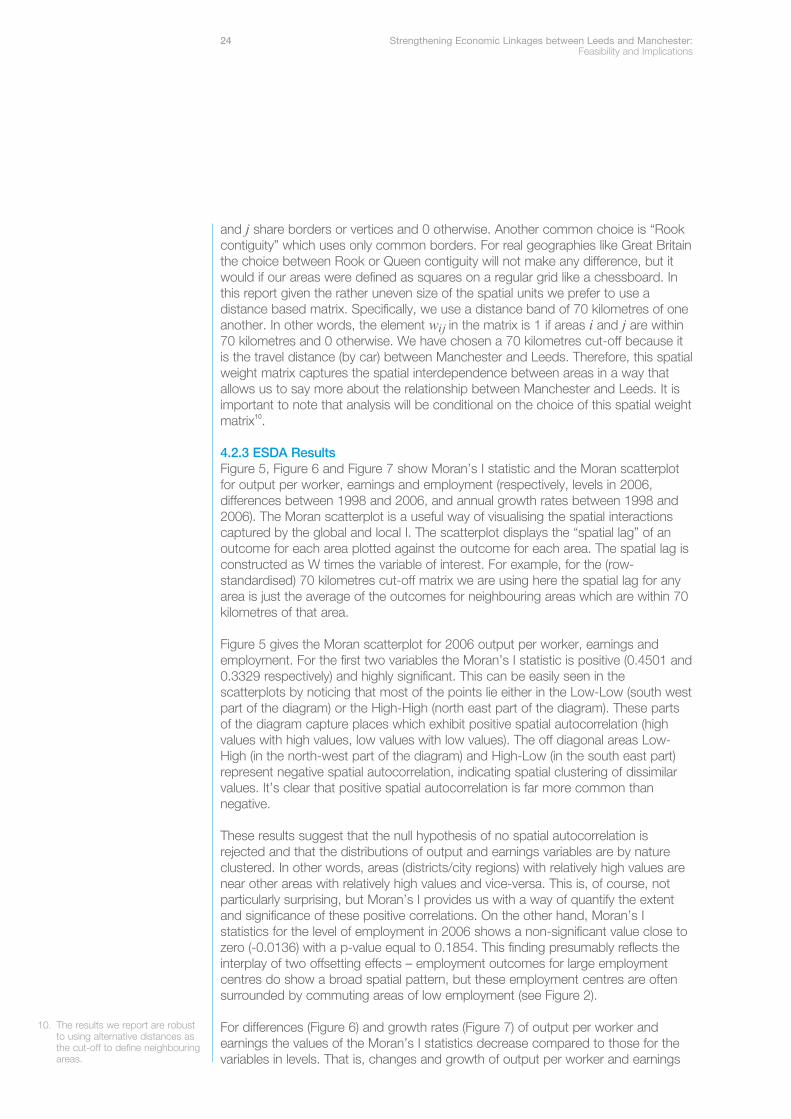
and j share borders or vertices and 0 otherwise. Another common choice is “Rookcontiguity” which uses only common borders. For real geographies like Great Britainthe choice between Rook or Queen contiguity will not make any difference, but itwould if our areas were defined as squares on a regular grid like a chessboard. Inthis report given the rather uneven size of the spatial units we prefer to use adistance based matrix. Specifically, we use a distance band of 70 kilometres of oneanother. In other words, the element wij in the matrix is 1 if areas i and j are within70 kilometres and 0 otherwise. We have chosen a 70 kilometres cut-off because itis the travel distance (by car) between Manchester and Leeds. Therefore, this spatialweight matrix captures the spatial interdependence between areas in a way thatallows us to say more about the relationship between Manchester and Leeds. It isimportant to note that analysis will be conditional on the choice of this spatial weightmatrix10.
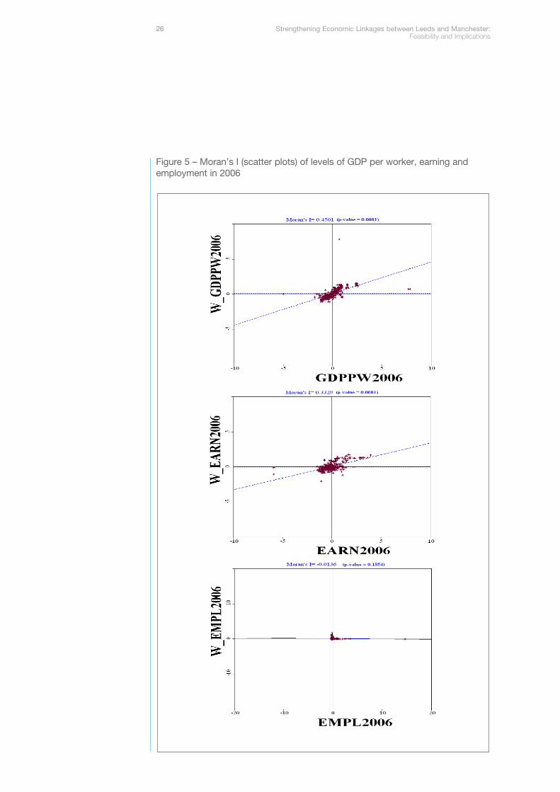
4.2.3 ESDA ResultsFigure 5, Figure 6 and Figure 7 show Moran’s I statistic and the Moran scatterplotfor output per worker, earnings and employment (respectively, levels in 2006,differences between 1998 and 2006, and annual growth rates between 1998 and2006). The Moran scatterplot is a useful way of visualising the spatial interactionscaptured by the global and local I. The scatterplot displays the “spatial lag” of anoutcome for each area plotted against the outcome for each area. The spatial lag isconstructed as W times the variable of interest. For example, for the (row-standardised) 70 kilometres cut-off matrix we are using here the spatial lag for anyarea is just the average of the outcomes for neighbouring areas which are within 70kilometres of that area.
Figure 5 gives the Moran scatterplot for 2006 output per worker, earnings andemployment. For the first two variables the Moran’s I statistic is positive (0.4501 and0.3329 respectively) and highly significant. This can be easily seen in thescatterplots by noticing that most of the points lie either in the Low-Low (south westpart of the diagram) or the High-High (north east part of the diagram). These partsof the diagram capture places which exhibit positive spatial autocorrelation (highvalues with high values, low values with low values). The off diagonal areas Low-High (in the north-west part of the diagram) and High-Low (in the south east part)represent negative spatial autocorrelation, indicating spatial clustering of dissimilarvalues. It’s clear that positive spatial autocorrelation is far more common thannegative.
These results suggest that the null hypothesis of no spatial autocorrelation isrejected and that the distributions of output and earnings variables are by natureclustered. In other words, areas (districts/city regions) with relatively high values arenear other areas with relatively high values and vice-versa. This is, of course, notparticularly surprising, but Moran’s I provides us with a way of quantify the extentand significance of these positive correlations. On the other hand, Moran’s Istatistics for the level of employment in 2006 shows a non-significant value close tozero (-0.0136) with a p-value equal to 0.1854. This finding presumably reflects theinterplay of two offsetting effects – employment outcomes for large employmentcentres do show a broad spatial pattern, but these employment centres are oftensurrounded by commuting areas of low employment (see Figure 2).
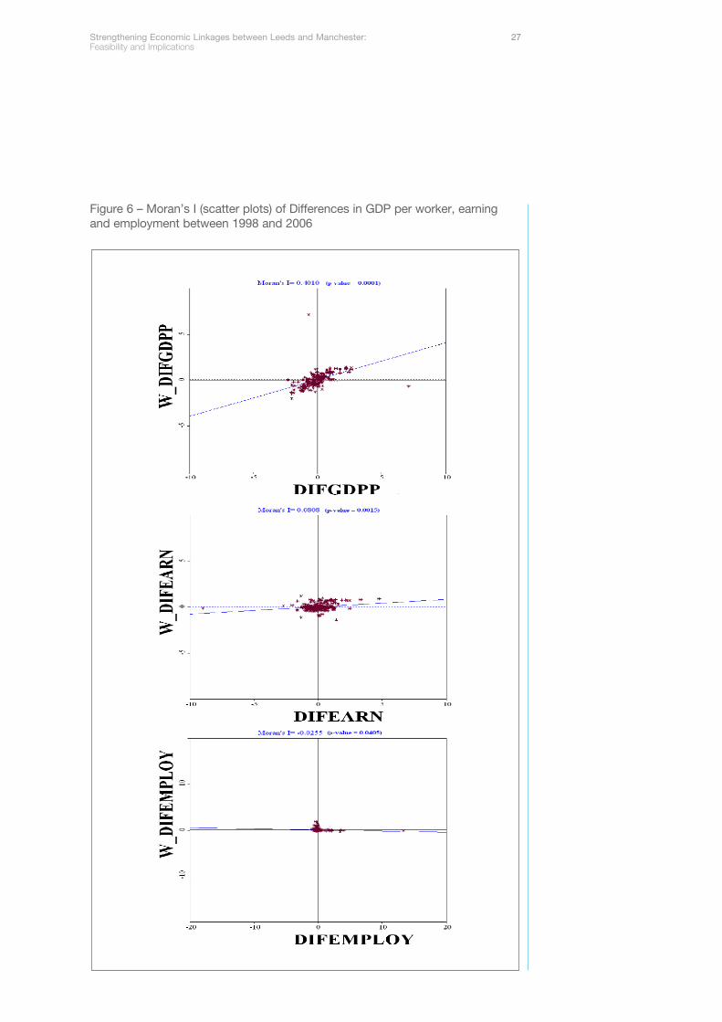
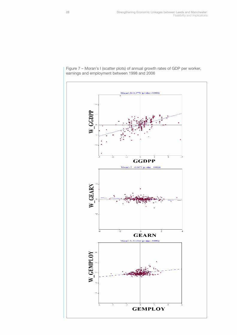
For differences (Figure 6) and growth rates (Figure 7) of output per worker andearnings the values of the Moran’s I statistics decrease compared to those for thevariables in levels. That is, changes and growth of output per worker and earnings
10. The results we report are robustto using alternative distances asthe cut-off to define neighbouringareas.
24 Strengthening Economic Linkages between Leeds and Manchester: Feasibility and Implications
show more of a random spatial pattern than levels. Interestingly, however, thedifference and growth rates of employment become positively statisticallysignificantly correlated at the 5% and 1% level, respectively. For difference in outputper worker between 1998 and 2006 (Figure 6), the Moran’s I statistic is positive andsignificant (0.4010) with a p-value equal to 0.0001. For differences in earnings theMoran’s I statistic is 0.0808 with a p-value equal to 0.0015. Finally, in Figure 7 weobserve that the null hypothesis of no spatial autocorrelation for growth rates ofemployment is rejected (p-value=0.0001) showing that the distributions of thisvariable is by nature clustered over the period 1998-2006.
In summary, large significant and positive values of Moran’s I reveal the presence ofspatial association of similar values among neighbouring areas in output per workerand earnings in 2006. However, when their differences and growth rates areanalyzed the values of the statistic decrease. The main finding to emerge at thispoint is that Moran’s I values in levels are higher than those for differences andgrowth rates. We now turn to the question of local associations and the specificquestion of the relative strength of the spatial correlation between Manchester andLeeds.
Strengthening Economic Linkages between Leeds and Manchester: 25Feasibility and Implications
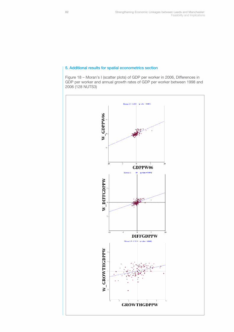
Figure 5 – Moran’s I (scatter plots) of levels of GDP per worker, earning andemployment in 2006
26 Strengthening Economic Linkages between Leeds and Manchester: Feasibility and Implications
Figure 6 – Moran’s I (scatter plots) of Differences in GDP per worker, earningand employment between 1998 and 2006
Strengthening Economic Linkages between Leeds and Manchester: 27Feasibility and Implications
Figure 7 – Moran’s I (scatter plots) of annual growth rates of GDP per worker,earnings and employment between 1998 and 2006
28 Strengthening Economic Linkages between Leeds and Manchester: Feasibility and Implications
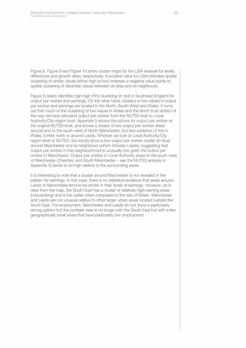
Figure 8, Figure 9 and Figure 10 show cluster maps for the LISA analysis for levels,differences and growth rates, respectively. A positive value for LISA indicates spatialclustering of similar values (either high or low) whereas a negative value points tospatial clustering of dissimilar values between an area and its neighbours.
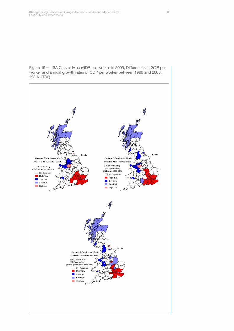
Figure 8 clearly identifies high-high (HH) clustering (in red) in Southeast England foroutput per worker and earnings. On the other hand, clusters of low values in outputper worker and earnings are located in the North, South-West and Wales. It turnsout that much of the clustering of low values in Wales and the North is an artifact ofthe way we have allocated output per worker from the NUTS3 level to Local-Authority/City-region level. Appendix 5 shows the picture for output per worker atthe original NUTS3 level, and shows a cluster of low output per worker areasaround and to the south west of North Manchester, but less evidence of this inWales, further north or around Leeds. Whether we look at Local-Authority/Cityregion level or NUTS3, the results show a low output per worker cluster (in blue)around Manchester and its neighbours (which includes Leeds), suggesting thatoutput per worker in this neighbourhood is unusually low given the output perworker in Manchester. Output per worker in Local-Authority areas to the south westof Manchester (Cheshire, and South Manchester – see the NUTS3 analysis inAppendix 5) tends to be high relative to the surrounding areas.
It is interesting to note that a cluster around Manchester is not revealed in thepattern for earnings. In this case, there is no statistical evidence that areas aroundLeeds or Manchester tend to be similar in their levels of earnings. However, as isclear from the map, the South-East has a cluster of relatively high-earning areas(unsurprising) and is the outlier when compared to the rest of Britain. Manchesterand Leeds are not unusual relative to other larger urban areas located outside theSouth East. For employment, Manchester and Leeds do not show a particularlystrong pattern but the contrast here is no longer with the South East but with a fewgeographically small areas that have particularly low employment.
Strengthening Economic Linkages between Leeds and Manchester: 29Feasibility and Implications
Figure 8 – LISA Cluster Map (levels of GDP per worker, earning and employmentin 2006)
30 Strengthening Economic Linkages between Leeds and Manchester: Feasibility and Implications
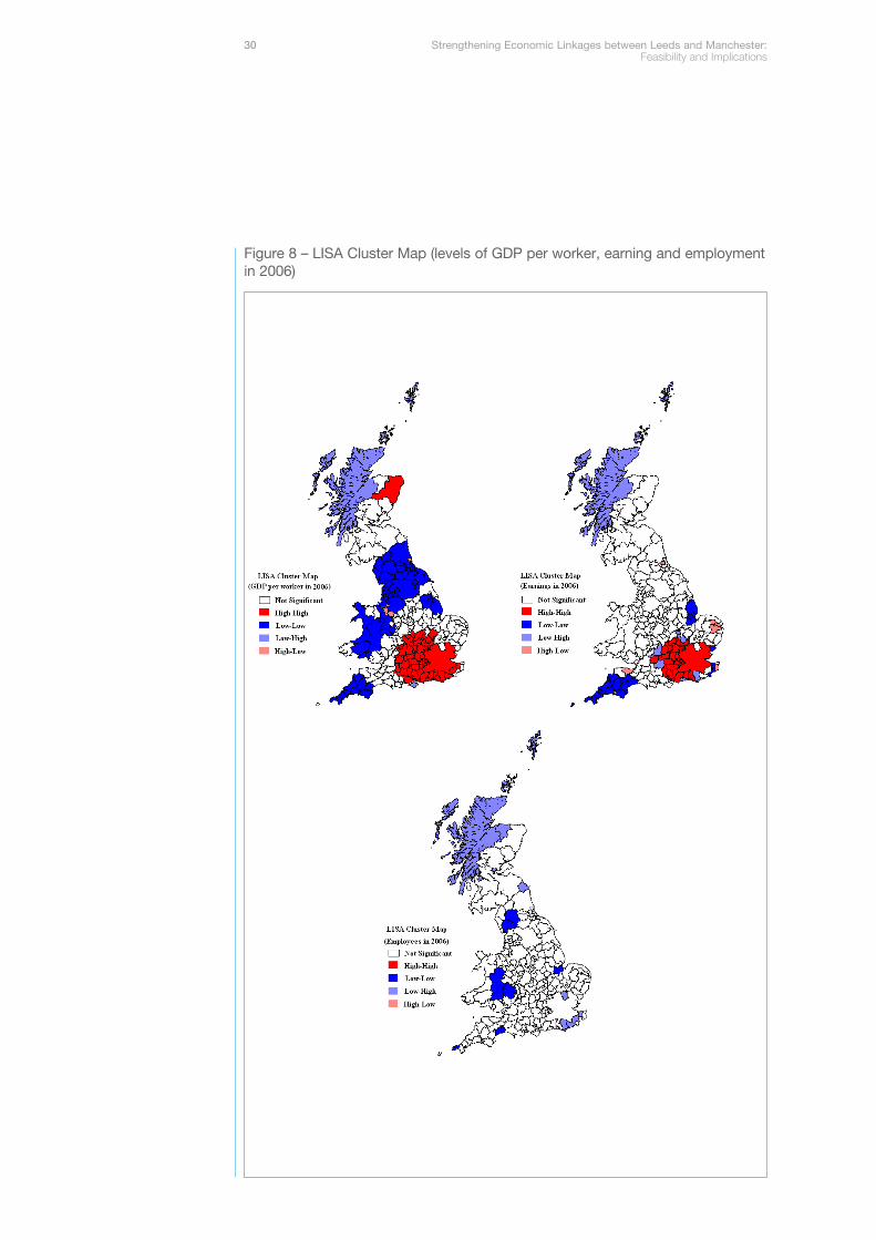
Figure 9 – LISA Cluster Map (Differences in GDP per worker, earnings andemployment between 1998 and 2006)
Strengthening Economic Linkages between Leeds and Manchester: 31Feasibility and Implications
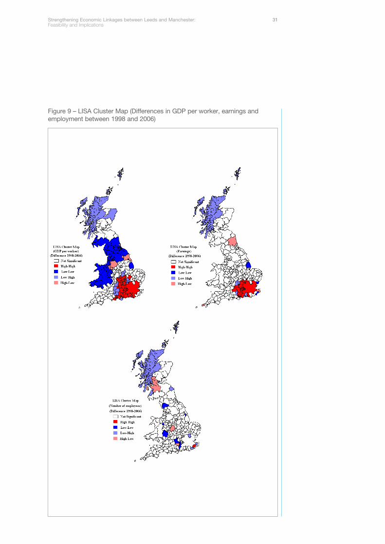
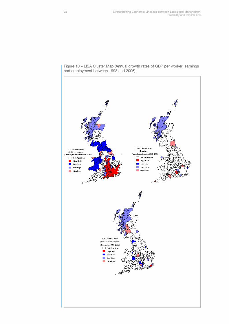
Figure 10 – LISA Cluster Map (Annual growth rates of GDP per worker, earningsand employment between 1998 and 2006)
32 Strengthening Economic Linkages between Leeds and Manchester: Feasibility and Implications
The patterns in Figure 8 show us where there are spatial clusters of high and lowvalues for the levels of output per worker, earnings and employment. But the moreinteresting question when considering economic linkages is whether there is atendency for these values to move together over time in neighbouring places. Toanswer this question, Figure 9 and Figure 10 show the cluster maps of differencesand growth rates of output per worker, earning and employment. Again, there areissues with allocating output per worker to Local-Authority/city-region level, soAppendix 5 provides a NUTS3 level analysis for comparison.
Here, the stand out point relating to output per worker around Manchester andLeeds can be observed in the first panel of Figure 9 (and second panel of Appendix5). Manchester and Local Authority areas to its south west (specifically SouthManchester) have moved in the opposite direction to their neighbours in terms ofchanges in output per worker. This is an unusual pattern relative to the rest ofBritain, and overall there is no evidence of a tendency for Manchester and Leeds tomove together in terms of change in output per worker. Again, the picture isdifferent for earnings and employment change, with no indication of any spatiallinkages in Local Authority areas around Manchester-Leeds, and little sign oflinkages anywhere else outside hotspots in the South East. Switching to growth (%change) as the metric in Figure 10, shows no spatial linkages between Manchester-Leeds and their neighbours in output per worker or earnings, although Manchesterappears as a low employment growth cool spot in the third panel. The mostinteresting point to take out of this analysis is that recent changes in output perworker in the Manchester City Region has been unusual positive relative to the restof Great Britain, but it has not been associated with similar changes in thesurrounding areas. More generally however, there are few signs that Manchester-Leeds are exceptional in their strength or weakness in spatial linkages. London andthe South East appear predominantly as the outlier in respect of strong positivespatial linkages relative to the rest of Great Britain. We now turn to try to understandwhat might have caused these patterns.
4.3 Spatial Econometric AnalysisSo far, we have examined the tendency for area outcomes to move with theirneighbours. We defined the spatial weight matrix (a 70 kilometres band) so thatManchester and Leeds count as “neighbours” and then we used exploratory spatialtechniques to examine whether their interaction is different from what we see inGreat Britain as a whole.
Given the results we obtained, it is interesting to attempt to further explore theextent to which measurable characteristics of areas drive these interactions. Sincewe have found that Manchester and Leeds are particularly unusual in terms of theirstrong spatial autocorrelation in output, weak correlation in terms of earnings andemployment and particularly weak in terms of some aspects of growth, it would beinteresting to know what characteristics of Manchester and Leeds might explainthis. As with our work on commuting, the strategy is to look at the nature of theserelationships across Great Britain to help identify the factors that cause the patternswe observe.
Strengthening Economic Linkages between Leeds and Manchester: 33Feasibility and Implications
We start our analysis with a basic equation:
Υ = Χ β + ε
where Y is the dependent variable for each area. Eight dependent variables areused:
(i) Output per worker in 2006;(ii) Earnings in 2006;(iii) Difference in output per worker between 1998 and 2006(iv) Difference in earnings between 1998 and 2006;(v) Difference in employment between 1998 and 2006;(vi) Annual growth rates of output per worker between 1998 and 2006;(vii) Annual growth rates of earnings between 1998 and 2006;(viii) Annual growth rates of employment between 1998 and 2006.
X is a matrix of area characteristics that may be important in explaining the behaviorof the dependent variables and is the error (or unexplained part of the dependentvariable). We include a group of variables which represent local sectoralcomposition, local occupation composition and education levels (all these variablesare in percentage terms) as well as the average age of the population. Seeappendix 4 for exact definitions.
Once we have estimated these equations we take the residual, or unexplained partof the dependent variable ε and examine whether it is spatially autocorrelated usingthe same approach as we did above. If we find it is not, then the spatial interactionthat we see between Manchester and Leeds is explained by them sharing similarcharacteristics. If we continue to observe spatial interaction in these residuals, thenwe would conclude that there is something specific about the interaction betweenManchester and Leeds that cannot be explained by observed characteristics.
34 Strengthening Economic Linkages between Leeds and Manchester: Feasibility and Implications
Strengthening Economic Linkages between Leeds and Manchester: 35Feasibility and Implications
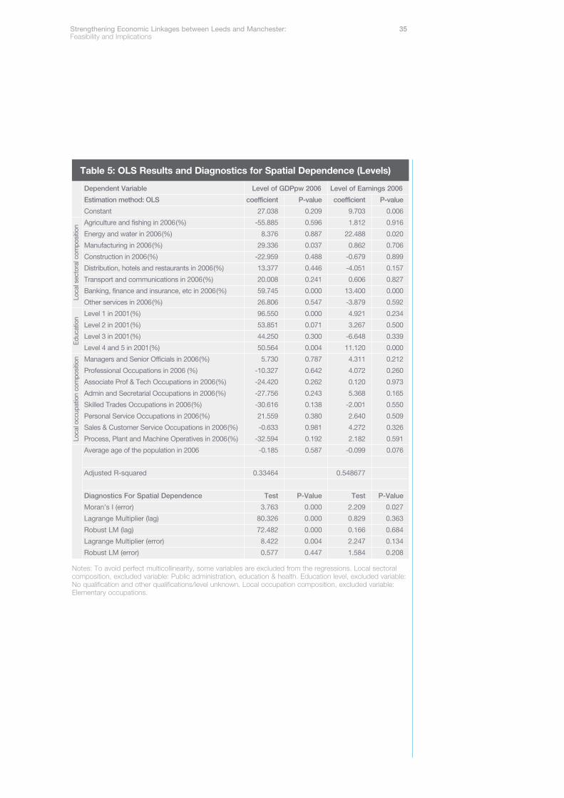
Dependent Variable Level of GDPpw 2006 Level of Earnings 2006
Table 5: OLS Results and Diagnostics for Spatial Dependence (Levels)
Notes: To avoid perfect multicollinearity, some variables are excluded from the regressions. Local sectoralcomposition, excluded variable: Public administration, education & health. Education level, excluded variable:No qualification and other qualifications/level unknown. Local occupation composition, excluded variable:Elementary occupations.
Loca
l sec
tora
l com
posi
tion
Edu
catio
nLo
cal o
ccup
atio
n co
mpo
sitio
n
36 Strengthening Economic Linkages between Leeds and Manchester: Feasibility and Implications
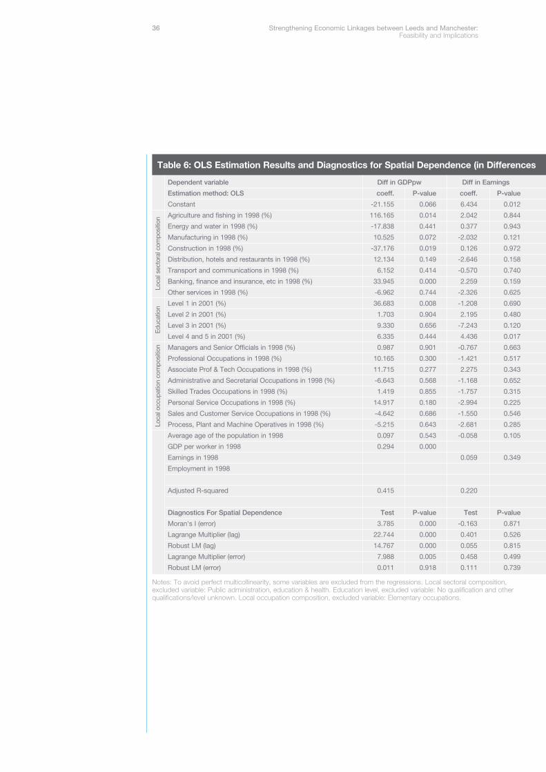
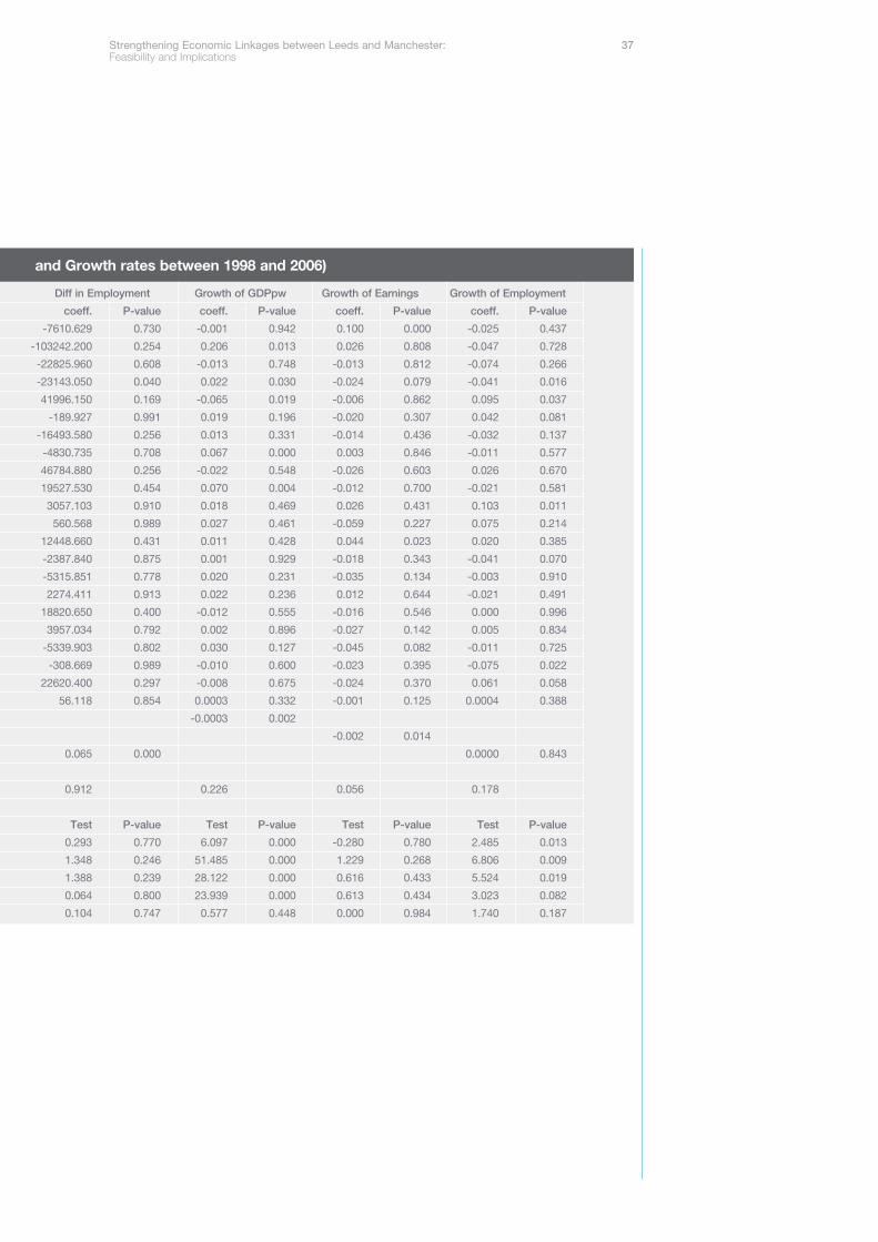
Table 6: OLS Estimation Results and Diagnostics for Spatial Dependence (in Differences
Notes: To avoid perfect multicollinearity, some variables are excluded from the regressions. Local sectoral composition,excluded variable: Public administration, education & health. Education level, excluded variable: No qualification and otherqualifications/level unknown. Local occupation composition, excluded variable: Elementary occupations.
Loca
l sec
tora
l com
posi
tion
Edu
catio
nLo
cal o
ccup
atio
n co
mpo
sitio
n
Strengthening Economic Linkages between Leeds and Manchester: 37Feasibility and Implications
Diff in Employment Growth of GDPpw Growth of Earnings Growth of Employment
Test P-value Test P-value Test P-value Test P-value
0.293 0.770 6.097 0.000 -0.280 0.780 2.485 0.013
1.348 0.246 51.485 0.000 1.229 0.268 6.806 0.009
1.388 0.239 28.122 0.000 0.616 0.433 5.524 0.019
0.064 0.800 23.939 0.000 0.613 0.434 3.023 0.082
0.104 0.747 0.577 0.448 0.000 0.984 1.740 0.187
and Growth rates between 1998 and 2006)
Table 5 and Table 6 report the Ordinary Least Square (OLS) results and diagnosticsfor spatial dependence. The way to read the table is to look for p-values less than0.05 or 0.10. These identify variables that have a statistically significant effect on thedependent variable at the 5% or 10% level, respectively. So, for example, for thelevel of output per worker, places with high shares of manufacturing and bankingsector have higher output per worker. Places with lower levels of education (level 1:e.g., Foundation GNVQ) and higher levels of education (levels 4 and 5: e.g., HigherDegree) also have higher output per worker. With the relatively broad occupationalclassifications that we use we do not observe any significant effect on output perworker or earnings (and similarly for age composition). There are certainly somepuzzles in these results, but our key interest is whether the spatial dependencebetween Manchester and Leeds remains or disappear after conditioning on theexploratory variables that, themselves, have very strong spatial or geographicpatterns.
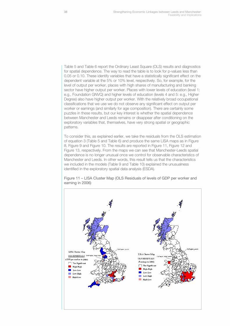
To consider this, as explained earlier, we take the residuals from the OLS estimationof equation 3 (Table 5 and Table 6) and produce the same LISA maps as in Figure8, Figure 9 and Figure 10. The results are reported in Figure 11, Figure 12 andFigure 13, respectively. From the maps we can see that Manchester-Leeds spatialdependence is no longer unusual once we control for observable characteristics ofManchester and Leeds. In other words, this result tells us that the characteristicswe included in the models (Table 9 and Table 10) explained the unusualnessidentified in the exploratory spatial data analysis (ESDA).
Figure 11 – LISA Cluster Map (OLS Residuals of levels of GDP per worker andearning in 2006)
38 Strengthening Economic Linkages between Leeds and Manchester: Feasibility and Implications
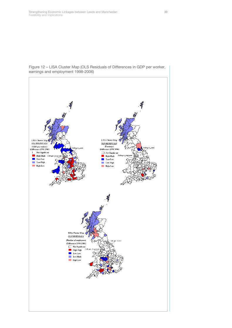
Figure 12 – LISA Cluster Map (OLS Residuals of Differences in GDP per worker,earnings and employment 1998-2006)
Strengthening Economic Linkages between Leeds and Manchester: 39Feasibility and Implications
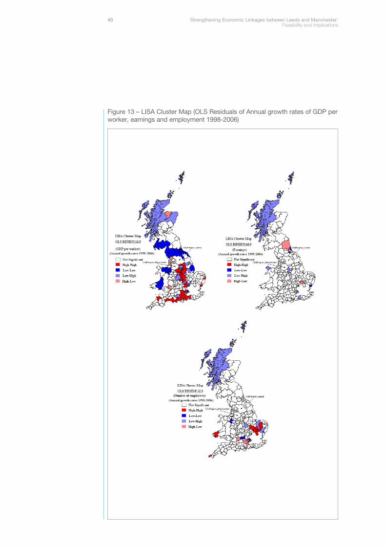
Figure 13 – LISA Cluster Map (OLS Residuals of Annual growth rates of GDP perworker, earnings and employment 1998-2006)
40 Strengthening Economic Linkages between Leeds and Manchester: Feasibility and Implications
4.4 Conclusions – Spatial Econometric Analysis
• Exploratory spatial econometric analysis indicates that there are some distinctspatial patterns in output per worker, and changes in output per worker aroundManchester and Leeds. In particular, South Manchester and areas to its southwest are unusual in the extent to which recent positive changes in output perworker have not been linked to positive changes in surrounding areas.
• More generally, for earnings, employment and growth in output per worker thereis little evidence of co-movement between Manchester-Leeds and theirneighbours. Manchester-Leeds is not unusual in this respect when judgedagainst other urban areas in Britain. Manchester-Leeds appears unusual whencompared to London and the South East, because this area exhibits unusuallystrong positive links in terms of levels and changes in economic indicators.
• Any differences from general GB patterns are explained by a few structural,economic characteristics of the two areas. As with commuting, this findingpoints away from social, cultural or similar factors as drivers of weak linkagesbetween the cities (although we do not study these factors directly). It suggeststhat other unexplained factors are unlikely to constrain Manchester and Leedsfrom following the general GB pattern.
• This analysis reminds us that the interactions between places are as muchoutcomes of the underlying structural characteristics of those places as they aredrivers of changes in those structural characteristics. Given the current industrialand skills structures of the Manchester and Leeds city regions the correlations interms of outcomes are about what we would expect.
• Overall, this suggests that structural change would be likely to play an integralpart in increasing the extent of observed interaction between the two city-regioneconomies.
Strengthening Economic Linkages between Leeds and Manchester: 41Feasibility and Implications
The work discussed so far describes and analyses existing interactions in terms of adirect measure of linkages (commuting) and outcomes (earnings, employment andoutput per worker). As we explained in the introduction we view this as both tellingus something about current behaviour and the feasibility of increasing interaction.We now turn to the possible impacts of increasing integration. In this section weconsider the agglomeration benefits of increased productivity focusing, in particular,on the functioning of labour markets.
Our starting point is the observation that, all else equal, larger places tend to havehigher productivity and wages. Economists refer to the productivity benefitsassociated with increased levels of economic activity as agglomeration economies(or benefits). At their broadest level, agglomeration economies occur whenindividuals and firms benefit from being near to others. We will refer to this as theeffect of better access to economic mass. This report focuses on agglomerationeconomies that arise in production. It is important to remember, however, that theremay be other benefits of agglomeration, for example in terms of consumption.
With this focus, agglomeration economies arise because of the production benefitsof physical proximity. Physical proximity to other firms, workers and consumers,may help firms in the day-to-day business of producing goods and services. Thisimplies that the productivity, of individual firms will rise with the overall amount ofactivity in other nearby firms, or with the number of nearby workers or consumers.Physical proximity may also facilitate the flow of ideas and knowledge leading firmsto be more creative and innovative. Higher productivity, in turn, tends to lead tohigher wages for workers.
The literature traditionally emphasises three sources of agglomeration economies:linkages between intermediate and final goods suppliers, labour market interactions,and knowledge spillovers. Input-output linkages occur because savings ontransaction costs means firms benefit from locating close to their suppliers andcustomers. Larger labour markets may, for example, allow for a finer division oflabour or provide greater incentives for workers to invest in skills. Finally, knowledgeor human capital spillovers arise when spatially concentrated firms or workers aremore easily able to learn from one another than if they were spread out over space.In this report, we are only concerned with the overall effect of increased access toeconomic mass. MIER (2008) includes a much more detailed discussion of thesources of different agglomeration economies and provides a review of the existingliterature.
Existing work for The Northern Way11 has followed Department for Transportguidance on evaluating the wider economic impacts of transport schemes toaddress this question. This approach uses estimates of the strength ofagglomeration economies, coupled with assumptions on the extent to whichintegration would increase local economy size to work out the productivity impactson different sectors of the economy. We use labour market data to try tounderstand whether this existing work captures all the likely impacts of increasedintegration.
It has been suggested that the size of the Manchester and Leeds economies mayhave negative implications for labour market outcomes, particularly for more highlyeducated workers, and that this may be an important factor in explaining their relativeunder performance12. To examine this possibility we use data on individual wages tosee how the level and growth of wages are affected by the size of the local labour
11. See Agglomeration SimulationExercise, Steer Davies Gleave(November 2006) for The NorthernWay; and Model Developmentand Results for The Northern Wayusing the South and WestYorkshire Dynamic Model, SteerDavies Gleave (December 2006).
12. See, for example, the ManchesterIndependent Economic Review’swork on skills which considersthis issue.
5. Agglomeration and labour markets
42 Strengthening Economic Linkages between Leeds and Manchester: Feasibility and Implications
market. This is just another way of trying to identify the overall agglomeration benefitsthat have been studied in the previous research referred to above.
In the academic literature it is increasingly recognized, however that the changingcomposition of the labour market may account for a large part of the overall positiverelationship between wages, productivity and city size. For example, it may be thatlarge cities tend to attract more educated workers. Because more educatedworkers also tend to earn more this leads to a positive relationship between city sizeand wages. In this scenario when we measure agglomeration economies by lookingat how wages change with city size we are capturing the fact that the compositionof the labour force changes with city size. Alternatively, it could be that larger citiesactually make workers more productive whatever their education level. That is, thereis a place-based effect whereby larger cities pay higher wages. Existing work onagglomeration economies (including that for the MIER, DfT and The Northern Way)has focused on assessing the overall impact of city size. In contrast, our researchassesses the extent to which these overall benefits arise from changing compositionas opposed to higher wages for existing workers. We then use our estimates,coupled with realistic assumptions about policy induced changes in transport costs,to assess the impact of increased integration on labour market outcomes. Thisallows us to paint a much richer picture of the potential sources of gains, thedistribution of benefits and the kinds of structural changes that might be needed toachieve them.
5.1 Methodology and DataTo assess the magnitude of overall agglomeration benefits we need to see howwages differ with city size. We then want to break these overall benefits down in tothose that come from changing composition versus those that come from place-based effects. To do this, we need to be able to look at the wage levels forindividuals who are otherwise identical but who happen to live in different cities.Ideally, we would do this by randomly allocating people across cities. In reality,fortunately, the UK government does not decide in which cities people live. Thiscreates a problem for us, however, because people are able to sort across cities innon-random ways. Imagine, for a moment, that we are able to observe everythingabout an individual (age, sex, education) that might affect their wage. Then, even inthe absence of random allocation across cities, we can still identify place effects onwages by comparing wages for people with identical observable characteristics whohappen to live in different places.
Unfortunately, even with quite detailed data, we cannot usually be certain that weare observing everything about an individual that might affect wages. For example,in the data that we use, we have no information on cognitive abilities or motivation.So when we compare two people with identical observed characteristics it may bethat the one with higher ability lives in the larger city and thus earns a higher wage.It is the unobserved individual characteristics (ability) that explains the higher wageof the individual in the larger city but we mistakenly attribute it to the effect of citysize. If, on average, higher ability individuals live in bigger cities, then we will find astatistical relationship between city size and wages even though city size has nodirect causal effect on wages. In this example, the relationship between city sizeand wages comes about instead because labour markets in bigger cities differ intheir ability composition from labour markets in smaller cities.
One way to get round this is to follow the same individual as they move acrosscities. Providing that ability is fixed over time if we see the same individual earning
Strengthening Economic Linkages between Leeds and Manchester: 43Feasibility and Implications
more in larger cities we may be more confident in attributing this to a place-basedeffect rather than a composition effect. Even then, we cannot rule out the possibilitythat something changed for the individual that both affected their earnings potentialand their choice of place to live. Still, in the absence of random allocation of people(or a policy change that as good as randomly assigns people) tracking individualsover time is the best that we can do to identify true place-based effects of changingcity size.
As is clear from this discussion we need data on individuals that providesinformation on where they work, on their wages and on the individual characteristicsthat might affect wages. We would also like to be able to follow individuals overtime, particularly as they move across cities. Such data is available from the NewEarnings Survey and the Annual Survey of Hours and Earnings (NES/ASHE).
We use data on individual wages calculated as the basic hourly wage fromNES/ASHE. Data on individual characteristics – age, age squared, gender andoccupation come from the same source. ASHE does not provide years of educationso we construct these using cohort of birth-by-SOC matching on data from theLabour Force Survey (LFS) which contains information on both occupations andeducation. The way that we do that is described in Appendix 1. Individualoccupation levels comes from NES/ASHE and are recorded using SOC1990 for1998-2001 and SOC2000 for 2002 onwards. Data on the characteristics of anindividual’s job (public sector, part time, collective agreement) also come fromNES/ASHE. NES/ASHE also includes the industry of occupation recorded usingSIC2003. The information on aggregate employment and the industrial structure ofan area comes from the Business Structure Database (BSD) which records thepostcode address, employment, and turnover of all VAT or PAYE registeredbusinesses in the UK. For the occupation structures of areas we need to aggregateup from the individual data in ASHE. Other area level variables – a Herfindahl indexof industrial diversity, shares of industry sectors at 1-digit level – are based on BSDdata. Finally, area proportions of workers belonging to high-skill and intermediate-skill groups are based on LFS data. More detail on the NES/ASHE dataset isprovided in the commuting section of this report.
We follow existing research for The Northern Way, Dft and the MIER by focusing onthe relationship between wages and ‘access to economic mass’ rather thanbetween wages and city size. The problem with the latter is that it requires us toimpose city boundaries on a map and talk about workers being located in aparticular city. In a sub-national context these boundaries are essentially arbitrary (atleast when it comes to the working of agglomeration economies). Measures ofaccess to economic mass treat space as continuous by taking into account accessto all other areas discounted by distance or transport cost to these areas, and avoidthe need to impose such arbitrary boundaries. We construct two measures ofaccess to economic mass as follows. The first measure is based on GeneralisedTransport Costs (GTC) when driving. We first use a mapping from postcodes towards to calculate total employment in each ward from the BSD. The access toeconomic mass for ward j in a given year is calculated by adding upcontemporaneous employment in all other wards using inverse-GTC (driving)weighting. This inverse-GTC weighting applies a weight of GTC -1
ij to theemployment in ward j, where GTCij is the ward-to-ward GTC for driving asdescribed in the commuting section. Therefore, a ward is assigned an aggregate ofemployment in other wards, with employment in more distant places contributingless than employment close by. The equation for the access to economic mass
44 Strengthening Economic Linkages between Leeds and Manchester: Feasibility and Implications
measure in ward i is thus: Α it = Σ empjt x GTC -1ij. To allow employment in ward i to
contribute to its own access to economic mass, we set GTCii = 0.5 x GTCi1 whereGTCi1 is the minimum ward-to-ward GTC for ward i (i.e. the “closest” ward). Eachworker is assigned the access to economic mass value equal to the ward in whichtheir employer is located13. Note that this index of access to economic mass isidentical to the effective density index used by Graham (2006) (although we preferto refer to it as a measure of access to economic mass or employmentaccessibility). Our second access to economic mass measure is calculated usingtrain GTC. We only have LA-to-LA GTC so LAs, rather than wards, are theunderlying unit used to construct the index. The index is otherwise constructed inan identical manner to the index based on driving GTC. For simplicity, we will referto the employment accessibility measure based on driving GTC as “CarAccessibility” and that based on train GTC as “Train Accessibility”.
5.2 ResultsWe start by considering a simple model that captures overall agglomerationeconomies, ignoring the distinction between composition and place-based effects.To do this, we run regressions that explain the wages of an individual as a functionof the access to economic mass at the individual’s work place:
ln (wit ) = αt + θ ln (Αit) + εit
where wit is individual i’s wage at time t, Αit is one, or both, of the access toeconomic mass variables described above, εit is a residual, αt is a time varyingparameter and θ a time invariant parameter (both to be estimated). The alphascapture the fact that wages tend to rise over time, while the theta captures theimpact of increases in access to economic mass (the impact assumed constantover our relatively short time period). Results are reported in Table 7. We report theestimated coefficient, the associated standard error, the R-squared (which tells usthe percentage of variation in wages that are explained by access to economicmass) and the number of observations.
In the first panel we report results using only Car Accessibility (column 1), then onlyTrain Accessibility (column 2) then both together (column 3). We see that whenentered separately, unsurprisingly, both are positively and statistically significantlyassociated with wages. When we include both together we find the effect of CarAccessibility is positive but insignificant while that of Train Accessibility is bothpositive and significant. At this stage, one shouldn’t read too much in to thedifference between the coefficients on the two measures. As we will see below thisdifference depends crucially on what other characteristics of individuals are beingcontrolled for in the regressions. The effect of access to economic mass remainsessentially unchanged if we drop all individuals that work in the London Travel toWork Area (column 4). Finally, for comparison we present results based on TTWAemployment rather than access to economic mass (column 5).
In terms of magnitudes, the coefficient on TTWA employment in column 5 is theeasiest to interpret. As it is in logs, the coefficient is an elasticity and tells us that a10% increase in TTWA employment is associated with a 0.7% increase in wages.This is consistent with the existing literature of the effect of city size on productivitywhich reports the effect of a 10% increase in city size varying from around 0.2% to2% with most under 1%. The coefficients on the access to economic massmeasures are harder to interpret because they are calculated using GTC weightingof employment across all wards (driving) and LAs (train). Taken at face value, the
13. While ASHE contains informationon both home and workpostcode, NES only provides thelatter so we need to base ourmeasure of access to economicmass on work rather than homelocation.
Strengthening Economic Linkages between Leeds and Manchester: 45Feasibility and Implications
coefficient of 0.344 for Train Accessibility implies that a 10% increase inemployment in all wards in Britain, or a 10% reduction in the GTC between all LocalAuthority areas in Britain, would increase wages by around 3.4%. For the moment,it is simplest to focus on how these coefficients change as we introduce individualcharacteristics. Later, however, we calculate changes in economic mass consistentwith proposed transport interventions which we then use to give a feeling for themagnitude of the effects on wages.
As we explained above, the problem with using these figures (and the othersavailable in existing studies on agglomeration effects in Manchester and Leeds) isthat our results so far do not distinguish between two different explanations of thepositive correlation between access to economic mass and wage. To recap, whatwe have called a people-based or composition-based explanation relies onindividuals who would be better paid where-ever they live choosing to work inplaces with higher access to economic mass. For example, high ability people maylive disproportionately in larger cities. The alternative, place-based, explanationwould attribute the effect directly to the place so that otherwise identical individualsearn higher wages in places with greater access to economic mass.
To separate out these effects, we need to control for the fact that individualcharacteristics that affect wages may be correlated with access to economic mass.To do this, we include these individual characteristics in our wage regressions togive:
ln (wit ) = αt + βΧ it + θ ln (Αit) + εit
where Χ it are individual characteristics, beta is a parameter to be estimated and allother notation is as before. Beta captures the effect of individual characteristics onwages leaving theta to capture the effect of access to economic mass aftercontrolling for the composition effects that we described above.
We have a large number of individual level variables that could be included in theregression. In order to separate people/composition-based effects from place-based effects we want to control for predetermined productive characteristics ofindividuals that are correlated with the economic mass of the cities in which theychoose to live. These characteristics – e.g. gender, age – arise independently of city
46 Strengthening Economic Linkages between Leeds and Manchester: Feasibility and Implications
Table 7: Regressions of wages on access to economic mass
Notes: All models have log hourly earnings as a dependent variable and the explanatory variables of interestare logarithms of car and train accessibility, or log TTWA employment. All estimations are base on panel datafor 1998-2007, and include year effects. Errors are clustered at the TTWA level. ***, **, * denote significanceat the 1%, 5% and 10% levels respectively.
size, but can become correlated with city size because individuals with differentproductivities sort into cities of different sizes. Clearly the sex of a worker isdetermined independently of access to economic mass even if males and femalesthen choose to live in different places so that sex is correlated with access toeconomic mass. A similar argument applies to age.
However, there are some characteristics of individual that may at least partly bedetermined by economic mass. For example, people in different places may haveaccess to different opportunities in terms of occupations. If good access toeconomic mass causes a person to choose a more productive (and higher paid)occupation (which is possible if agglomeration economies cause some occupationsto be more prevalent in big cities) then we may want to attribute the resulting effecton wages to access to economic mass not to occupation. Controlling foroccupation in our wage regressions will yield estimates of the effect of economicmass that net-out any effects arising from the occupational choice of individuals.Similarly, if big cities encourage development of human capital (education),controlling for individual education in our regressions nets-out any wage effects onindividuals arising via the educational choices of individuals. Similar arguments applyto industry choices.
An additional challenge is that an association between composition and economicmass could arise because, historically, more productive workers tend to live closertogether. It could also arise because better transport connections have evolvedbetween labour markets with more productive workers. The reason we need bevery cautious here is that the direction of causality may not run from economicmass to labour market composition, but in the opposite direction: Productive labourmarkets encourage better transport linkages. If this is the case then improvingtransport linkages will not be effective in changing the composition of the labourmarket or raising productivity. Therefore the estimates in Table 7 are upward biasedand the economic benefits that they imply will never be fully realised by improvingtransport connections or otherwise increasing economic mass.
These issues complicate our analysis. On the one hand, we want to purgeestimates of compositional biases arising from the sorting of more productivepeople into places of higher economic mass. For example, individuals who chooseto work in finance may be highly paid in finance in whatever size city they worked.But finance jobs tend to be located in places of high economic mass, so there is acorrelation between economic mass and individual wages arising through thesorting of finance workers into dense city centres. It would be wrong in this firstcase to attribute the individual’s higher wage to the fact that they work in a denseplace rather than that they work in finance. To avoid this type of bias, we need tocontrol for the industry in which an individual works.
We also want to control for industry, occupation and other characteristics to try topurge our estimates from bias arising from the potential reverse causality runningfrom productive labour markets to economic mass discussed above. For example,London’s productive finance sector probably started life in response to London’sposition as a port and trade centre. London’s economic mass and transportinfrastructure grew as a consequence. Therefore, it would be wrong to attribute allLondon’s productivity and its higher proportion of more educated workers to theexistence of economic mass and transport infrastructure, since it is the productivitywhich has caused infrastructure and mass to grow.
Strengthening Economic Linkages between Leeds and Manchester: 47Feasibility and Implications
On the other hand, a non-financial worker who lives in a big city with a largefinancial sector may be encouraged to work in finance because of the prevalence ofwell paid financial jobs. If we are interested in the overall effect of economic masson individual wages, we would like to include this effect that works through industrychoice. In this second case, we do not necessarily want to control for industry inour wage regressions, because controlling for industry will eliminate one of thechannels through which economic mass acts on wages.
In short, in our wage regressions we want to control for individual variables that canbe regarded as predetermined, in the sense that they are not determined by accessto economic mass in the city in which a person currently lives and works. But thereare some characteristics like occupation, education and industry which are partlypredetermined, but partly determined by the economic mass of the city in which aperson lives and works. If we control for all these factors, we control for allcompositional effects arising both through sorting (which we want to eliminate), andthrough changes in individual characteristics induced by economic mass (which wedo not necessarily wish to eliminate).
One modelling approach would be to control for all characteristics to obtain a fullyspecified model of wage determination, and then estimate separate models whichdeal with the mechanisms by which economic mass determined occupation,industry and education choice probabilities. This challenging undertaking is beyondthe scope of this report.
The more feasible approach which we employ here is simply to estimate wageequations using various individual control variable sets, whilst recognising thatcontrolling for variables that are partly determined by economic mass is likely toyield lower bounds to the overall impact of economic mass on individual wages,whereas failing to control for predetermined characteristics is likely to upward biasour estimates. In reality, of course, we do not usually know which characteristics arepre-determined and which are channels through which access to economic massoperates. We proceed by introducing variables starting with those that are mostlikely to be pre-determined and then adding in variables where we are less certain.
We start by introducing sex, age and age squared which, as argued above, arecertainly predetermined. Results for the coefficient on the two access to economicmass measures are reported in Table 8, while we report the full results in Table 1 inAppendix 6. Column 1 just replicates the results from Table 7 where we onlyconsider the effect of access to economic mass and do not control for anyindividual characteristics. Column 2 shows what happens when we control for sex,age and age squared (sometimes thought of as capturing the effect of experience).The coefficient on Car Accessibility drops while that on Train Accessibility increases.Taken literally this tells us that people who work in places with good CarAccessibility tend to be male and middle aged. We know this because the fall in thecoefficient on Car Accessibility means that we must have included characteristicsthat must be positively correlated with both wage and Car Accessibility. Middle ageand being male are the individual characteristics positively associated with wages(see Table 1 in Appendix 5) so it must be these characteristics that are associatedwith higher Car Accessibility. In contrast, the increase in the coefficient on TrainAccessibility suggests the opposite. In fact, neither of the changes in coefficient arestatistically significant so, although these patterns arguably make sense one shouldnot read too much in to the changes.
48 Strengthening Economic Linkages between Leeds and Manchester: Feasibility and Implications
The next individual characteristic that we include is education. Although there issome evidence linking educational outcomes to access to economic mass thecausal effect is not large (if the effect is causal at all). Given our rather aggregatedskills classification we would argue it makes sense to see education aspredetermined. However, as column 3 makes clear, sorting means that education isquite strongly correlated with access to economic mass, at least for TrainAccessibility. Again, the interpretation of this is that higher educated workers getpaid higher wages and tend to live in areas with higher access to economic massby train. Once we control for this the association between wages and TrainAccessibility is significantly weakened.
Next we introduce variables to control for occupation, whether the individual worksin the public sector, works part time and is subject to a collective pay agreement.We could think of these characteristics as associated with either the individual orthe job. If the latter, it is a little harder to be certain that these characteristics arepredetermined. Fortunately this issue is moot as introducing these controls has littleaffect on the coefficients on the two access to economic mass variables (althoughthe effect is slightly larger for Car Accessibility) as can be seen by looking at theresults in column 4. A similar story applies with the introduction of industry controlsas can be seen from results reported in Column 5.
To summarise the results so far, when we control for composition based on theobservable characteristics of individuals (and jobs) the effect of access to economicmass is reduced by somewhere between a quarter and a third.
We can go one step further in our attempt to control for confounding factors thatmight be driving the relationship between access to economic mass and wages. Sofar, we have only controlled for the observable characteristics of individuals (thingsfor which we have data in ASHE). Given that we observe individuals over time,however, we can use panel data techniques to control for unobservablecharacteristics of individuals that might be positively associated with both wagesand access to economic mass. For example, as explained above, higher abilityindividuals will likely get higher wages and may also tend to live in larger cities. Asability is not recorded in our data, we would attribute the positive correlationbetween city size and wages to city size, when it was actually due to the sorting ofhigher ability individuals in to larger cities. To allow for this possibility, we estimate
Strengthening Economic Linkages between Leeds and Manchester: 49Feasibility and Implications
1 2 3 4 5 6 7
ln Car Accessibility 0.084 0.074 0.071 0.054 0.046 0.069*** 0.070***
Table 8: Regressions of wages on access to economic mass and othervariables
Notes: All models have log hourly earnings as a dependent variable and the explanatory variables of interestare logarithms of car and train accessibility variables. All estimations are based on panel data covering years1998-2007, and include year effects. Column [1] has no controls; [2] adds age, age squared and gender; [3]adds years of education; [4] adds occupational characteristics (1-digit level) and dummies for part-time,public sector and collective wage agreement); [5] adds 1-digit industry controls; [6] adds individual fixedeffects; [7] adds area level characteristics as described in the text. Standard errors are clustered at the travel-to-work area level. ***, **, * denote significance at the 1%, 5% and 10% levels respectively.
the model as above, but we now include individual fixed effects to control for timeinvariant unobservables. This implies that the effects of access to economics massare estimated from individuals that move over time (otherwise, for individuals that donot move, we cannot be sure whether the higher wages are something to do withthat individual or something to do with the place in which they live). Thespecification is thus:
ln (wit ) = αt + βΧ it + θ ln (Αit) + λi + εit
where everything is as defined before, except for the inclusion of individualunobserved fixed effects λi.
As can be seen from Column 6 in Table 8, the effect on the coefficients on themeasures of access to economic mass are considerable. The change is mostobvious for Train Accessibility where the coefficient is decreased by a factor of 3. Infact, the coefficient on Train Accessibility reduces sufficiently that the coefficient onCar Accessibility is now larger (although not significantly so). There is a further, moresubtle, impact on the coefficient on Car Accessibility. Looking at the standard errorswe see that the increase in the coefficient combined with a decrease in thestandard error makes Car Accessibility significant for the first time. Economistswould generally consider these results that control for both the observed andunobserved characteristics of individuals as providing the best estimate of therelationship between wages and access to economic mass controlling forcomposition. It is sensible to view these coefficients as capturing the upper boundof the likely effect on individuals who do not change sex, age, education etc as aresult of increasing access to economic mass. In short, once we allow forcomposition, both Car and Train Accessibility are positively related to wagesalthough the relationship is much weaker than suggested by our initial results thatdid not adjust for composition.
In the results reported so far, we only allow for place-based effects to be explainedby access to economic mass. It is, of course, possible that other areacharacteristics that are positively correlated with both access to economic massand wages might actually be the source of place-based effects. To consider this wecalculate a number of additional area based characteristics that might potentially beassociated with wages. Following Wheeler’s (2008) work on wages growth for theUS these include a measure of TTWA industrial diversity and occupational diversityto allow for the fact that diversity might be more important for wages than size perse. Industrial diversity of a TTWA j is calculated using a Herfindahl index: Σj(Eijt / Eit)2 where j is two digit industry, i is TTWA and t is year. Occupationaldiversity is an analogous measure using 2-digit occupational code-level employmentinstead of SIC. Although we cannot include a measure of access to economic massdisaggregated by skills (see the discussion above) we can include the share of highand intermediate skills in TTWA j’s working age population (with low skills theomitted category). Finally, we include measures of average TTWA industry shares(two digit) to see if the TTWA-wide industrial structure makes any difference.
Column 7 shows what happens to the coefficients on the two access variableswhen we include these additional area characteristics. The effect of Car Accessibilityis essentially unchanged, while that of Train Accessibility falls somewhat further.Results reported in Appendix 6 shows that TTWA percentage high skills and theshare of activity in Other Services are the only two area characteristics that have asignificant effect on wages. These appear, perhaps unsurprisingly, to be positively
50 Strengthening Economic Linkages between Leeds and Manchester: Feasibility and Implications
correlated with Train Accessibility which leads to overall reduction in the coefficienton that measure of accessibility. Of course, these results may partly reflect the factthat large places attract lots of skilled workers. There is an active debate in theeconometric literature about whether it is appropriate to control for the channelsthrough which an explanatory variable might impact outcomes at the same time astrying to identify the overall effect of the explanatory variable (see Angrist and Pishke2009). Without more evidence on the channels, and given that the coefficients onthe access variables do not change too markedly, we prefer to use the results inColumn 6 (ignoring other area characteristics) to assess the likely impact of thecounterfactuals described below. We note that our results in column 7 providesome preliminary evidence that part of these effects may work through increasingthe proportion of high skill.
Results reported in Table 9 show what happens when we exclude all individualsworking in London. The overall story is much as before. Car Accessibility has aninsignificant effect on wages, while Train Accessibility is significant (column 1).Adding in observable characteristics of individuals leaves the coefficient on CarAccessibility essentially unchanged while decreasing that on Train Accessibility(columns 2-5). As before, introducing individual fixed effects to control forunobservable characteristics more than halves the effect of Train Accessibility, whilemaking the effect of Car Accessibility positive and significant (column 6). Additionalarea controls make Car Accessibility insignificant and slightly reduce the effect ofTrain Accessibility. As before, our preferred specification is column 6 which showsthat excluding London does not make that much difference to the Train Accessibilitycoefficients that are the main focus of our counterfactual analysis below.
Finally, we can consider whether these effects differ depending on the skill level ofworkers. We are limited in what we can do here, because our measures ofeconomic mass are based on employment from the IDBR which only providesemployment classified by industry (not skill or occupation). This prevents us fromrecalculating our measures of access to economic mass based on employmentsplit by skill. Instead, we simply run our regressions separately for each skill groupcontinuing to use access to economic mass based on overall employment. Table10 shows the results for the three skill groups for our preferred specification(including individual fixed effects) and when we introduce area characteristics. It isinteresting to note that the lower skilled (group 1) benefit from Car Accessibility, butnot Train Accessibility. The highest skilled (group 4) benefit from both, although theeffect of Car Accessibility is still slightly larger. The proportion of high skilled in thearea has such a strong impact on the highest skilled that it essentially explains all ofthe effect of increased access to economic mass so that both access variables areinsignificant once we introduce additional area controls. We use the average effects
Strengthening Economic Linkages between Leeds and Manchester: 51Feasibility and Implications
1 2 3 4 5 6 7
ln Car Accessibility -0.040 -0.046 -0.011 -0.014 -0.015 0.017* 0.007
Table 9: Regressions of wages on access to economic mass and othervariables excluding London
Notes: Regressions as in Table 8. but excluding observations for London TTWA.
in what follows, ignoring the individual channels through which the effects mightoperate and ignoring the fact that the differences might differ somewhat acrossindividuals. The results in Table10 do suggest, however, that the effects ofimproving both Car and Train Accessibility may actually be slightly stronger for thosewith intermediate level skills while higher skill gain less and lower skill may notbenefit from increased Train Accessibility at all.
5.3 The labour market impacts of closer integrationWe can now use our results to assess the labour market impact of improvingaccess to economic mass. To do this we construct a number of counterfactualaccess to economic mass measures based on several different scenarios: (1) a 40minute reduction in train travel time between Leeds and London; (2) a 40 minutereduction in train travel time between Leeds and London; (3) a 20 minute reductionin train travel time between Manchester and Leeds; (4) a 1% reduction in train traveltimes within Leeds and within Manchester; (5) a 1% reduction in train travel timesbetween Manchester and Leeds; (6) and (7) as for (4) and (5) but for driving times;(8) and (9) a 10% increase in employment in all LAs in Manchester and Leeds (withthe effects on Car Accessibility and Train Accessibility reported separately). In thefirst three scenarios we also allow for the second round (or knock on) effects onjourneys between LAs not directly affected (e.g. Liverpool to Hull) that may seeimproved journey times as a result of the improved network. For the final fourtransport scenarios we just assess the impact of the first round effects. We do notview any of this as a serious transport modeling exercise, but instead use it to helpquantify the effects and identify key messages emerging from our analysis.Appendix 2 gives more details on the construction of counterfactuals, while Table11 reports the percentage changes in access to economic mass for each of thecounterfactuals. To translate these percentage changes in access to economicmass in to changes in wages we multiply by the relevant coefficients on Car andTrain Accessibility that we have estimated and reported in Table 8. Because thechange in economic mass for each LA will be multiplied by the same coefficient, theimpact on wages is proportional to the change in access to economic mass. Thismeans that the figures in Table 11 allow us to assess the relative magnitudes andthe distribution of the impacts of different types of changes.
Starting with the first two columns we see, unsurprisingly, that the impact of aLeeds-London reduction in train times is felt disproportionately in Leeds.Manchester LAs do benefit somewhat because the journey time matrix that wehave at our disposal suggests that for all Manchester LAs some journeys to LAs
52 Strengthening Economic Linkages between Leeds and Manchester: Feasibility and Implications
Skill group 1 Skill groups 2-3 Skill group 4
FE FE+Area FE FE+Area FE FE+Area
ln Car Accessibility 0.054*** 0.049*** 0.074*** 0.076*** 0.049*** 0.036
Table 10: Regressions of wages on access to economic mass and othercontrol variables split by skill group.
Notes: Regressions dividing by skill groups. FE reports coefficients from a regression including a full set ofindividual controls and is equivalent to specification [6] in Table 8. FE+Area adds a full set of areacharacteristics and is equivalent to specification [7] in Table 8. ***, **, * denote significance at the 1%, 5%and 10% levels respectively.
elsewhere in Great Britain become faster if they use the new faster Leeds-Londonsegment (see the section on counterfactuals in the appendix for more discussion ofthis). Similarly all Leeds LAs benefit from improved Manchester-London journeytimes but the effects are relatively small compared to the benefits to ManchesterLAs. In line with existing work for The Northern Way, the proportionate benefits are,overall, larger for Leeds (in column 1) than for Manchester (in column 2) becauseexternal accessibility is more important for the smaller economy. The differentialimpact of a 20 minute Manchester-Leeds travel time reduction is consistent withthis overall pattern, although it is clear that the most directly affected journeysbenefit most (e.g. Manchester and Leeds). The impact on accessibility of within cityGTC reductions are always larger than for between city GTC reductions. This is truefor both Train and Car Accessibility. It is beyond the scope of this report to assesswhether between or within GTC reductions are equally achievable but we providethe coefficients so that they can be used in future work to assess the likely impact ifsuch figures become available for specific schemes. Finally, we see that 10%increases in population for all LAs have a fairly uniform effect on accessibility with,unsurprisingly, central LAs tending to see larger increases in access to economicmass in response to these changes.
Strengthening Economic Linkages between Leeds and Manchester: 53Feasibility and Implications
Table 11: Percentage change in access to economic mass for differentcounterfactuals
Notes: Table shows percentage change in access to economic mass from a 40 minute reduction in trainjourney time Leeds-London (L-Lon -40m); 40 minute reduction Manchester-London (M-Lon-40m); 20 minutereduction Leeds-Manchester (L-M-20m); Within and Between train GTC reductions of 1% (WT, BT -1%);Within and Between driving GTC reductions of 1% (WC, BC, -1%) and population plus 10% using train andcar (TP, CP +10%). WC, BC and CP use LA-to-LA driving GTC, all others based on train GTC. CR indicatesCity-Region (L=Leeds, M=Manchester)
We now turn to the impact on wages obtained by multiplying the percentagechanges in accessibility by the relevant coefficients on Car and Train Accessibilitythat we have estimated and reported in Table 8. Table 12 works through theexample of a 20 minute reduction in train journey time between Manchester andLeeds (which happens to deliver the largest impact on wages of any of theexercises we consider). The column marked L-M -20m gives the percentagechange in Train Accessibility and just replicates column 3 of Table 11. The firstcolumn reports the total effects of this change (including any compositionalchanges). These range from a 2.7% increase in wages in Wakefield to a 1.06%increase in Tamefield. Column 2 shows what happens as we control for age andsex. Consistent with the discussion above, the estimate of the percentage wageeffect increases slightly because the coefficient on Train Accessibility is slightlyhigher (for convenience we repeat these coefficients in the last row of the table).Column 3 controls for education which leads to the first big reduction in theestimated size of the effect. Columns 4 and 5 show smaller changes as we firstintroduce occupation and then industrial controls. Finally column 6 shows the largereduction when we allow for unobservable individual characteristics. As a remindercolumn 6 is our preferred estimate of the impact of increased accessibilitycontrolling for the effects of composition. We see the results range from a high of0.50 of a percent for Wakefield to a low of 0.20 of a percent for Tameside. As isclear, compositional changes account for the vast majority of the estimated overallimpact on wages.
We view this as the fundamental policy message to emerge from our work onlabour markets: most of the overall agglomeration gains come from the changingcomposition of labour markets not from improved wages for those that do notchange education, occupation, industry or ability in response to increasedaccessibility. As the composition of the Manchester-Leeds economies shiftstowards higher educated, higher ability workers average wages will rise bysomewhere between 1.06% (Tameside) and 2.65% (Wakefield). But the gains toexisting workers who do not change their characteristics in response to increasedintegration are considerably smaller. We return to the implications of this in ourconclusions.
54 Strengthening Economic Linkages between Leeds and Manchester: Feasibility and Implications
5.4 Results: wage growthTo reiterate, our results so far suggest that any significant impact on wage levelsfrom greater integration of Manchester and Leeds labour markets come mostly fromchanging the composition of individuals and partly from changing the compositionof work via effects on industrial structure and occupation. The effects on workerswho are unable to change individual characteristics (education, ability) are quitesmall. In this sub-section we focus on the related question of whether access toeconomic mass plays a role in driving individual wage growth rather than levels.That is, we consider the possibility that increased access to economic mass is moreimportant for understanding the dynamics of the labour market. That is, we addressthe possibility raised by some commentators that the problem for Manchester andLeeds is that there smaller access to economic mass means that labour marketsare “thin” preventing workers from moving around between jobs as a way ofachieving faster wage growth.
The sample of individuals that we use to study wage growth is essentially the sameas the one that we use for the results reported above (we apply some additionaltrimming to eliminate very large growth rates). The dependent variable is annualised
Strengthening Economic Linkages between Leeds and Manchester: 55Feasibility and Implications
L-M
LAD NAME CR 20m 1 2 3 4 5 6
Bradford L 6.59 1.70 1.83 1.14 1.09 1.12 0.32
Calderdale L 6.05 1.56 1.68 1.05 1.00 1.03 0.30
Craven L 6.3 1.63 1.75 1.09 1.04 1.07 0.31
Harrogate L 6.98 1.80 1.93 1.21 1.15 1.19 0.34
Kirklees L 6 1.55 1.66 1.04 0.99 1.02 0.29
Leeds L 9.75 2.52 2.70 1.69 1.61 1.66 0.48
Selby L 6.51 1.68 1.80 1.13 1.07 1.11 0.32
Wakefield L 10.26 2.65 2.84 1.77 1.69 1.74 0.50
Bolton M 6.17 1.59 1.71 1.07 1.02 1.05 0.30
Bury M 6.24 1.61 1.73 1.08 1.03 1.06 0.31
Congleton M 6.29 1.62 1.74 1.09 1.04 1.07 0.31
High Peak M 5.22 1.35 1.45 0.90 0.86 0.89 0.26
Macclesfield M 7.84 2.02 2.17 1.36 1.29 1.33 0.38
Manchester M 10.07 2.60 2.79 1.74 1.66 1.71 0.49
Oldham M 4.56 1.18 1.26 0.79 0.75 0.78 0.22
Rochdale M 4.34 1.12 1.20 0.75 0.72 0.74 0.21
Salford M 4.42 1.14 1.22 0.76 0.73 0.75 0.22
Stockport M 7.62 1.97 2.11 1.32 1.26 1.30 0.37
Tameside M 4.12 1.06 1.14 0.71 0.68 0.70 0.20
Trafford M 6.4 1.65 1.77 1.11 1.06 1.09 0.31
Vale Royal M 6.21 1.60 1.72 1.07 1.02 1.06 0.30
Warrington M 6.86 1.77 1.90 1.19 1.13 1.17 0.34
Wigan M 6.47 1.67 1.79 1.12 1.07 1.10 0.32
Multiply percentage change by 0.25800 0.27700 0.17300 0.16500 0.17000 0.04900
Table 12: Percentage change in wages for a 20 minute reduction inManchester-Leeds train time
Notes: Table shows percentage change in accessibility for a 20 minute reduction in train journey timesbetween Manchester and Leeds (L-M-20m). Column [1] shows total effects including any compositionalchanges; [2] controls for age, age squared and gender; [3] controls for years of education; [4] controls foroccupational characteristics (1-digit level) and dummies for part-time, public sector and collective wageagreement); [5] controls for 1-digit industry; [6] controls for individual fixed effects. The final row correspondsto the coefficients in columns [1] to [6] reported in Table 8.
percentage wage growth over the period of observation of the individual: ln (wT - wt0 )/(T - t0 ) where wt0 is the individuals’ annual wage in the first year theyare observed and wT is the wage in the final year. The percentage wage growth isnormalized by the number of years T - t0 over which the individual is observed toallow for the fact that we observe different individuals for different lengths of time.
We work through exactly the same set of specifications as we did for wages. Thatis, we start by introducing controls for sex, age and age squared. We then controlfor education followed by “job” characteristics (occupation, part time, public sector,collective agreement) and industry. Finally, we control for other area characteristics.The access to economic mass and area variables are constructed as above. Notethat, as we only have one observation of wage growth for each individual we cannotinclude individual fixed effects to control for unobserved ability (as we did in ourpreferred specification above). We discuss the likely implications of this furtherbelow.
Because we are looking at wage growth over a period of years we need to decidewhich variables we measure at the start of the period and which we allow to varyover time. Sex is obviously fixed and, without loss of generality, we can alsomeasure age and experience at the start of the period (because age increaseslinearly across time). For the remaining individual and job characteristics we simplytake the average over the period for which we observe the individual. We also timeaverage accessibility and area characteristics for each individual (thus allowing forthe fact that individuals may move across TTWAs over time).
We start, as with the level of wages, by regressing growth in wages on the accessto economic mass variables separately and together. Results are reported in Table13 where, once again, for comparison we also include the coefficients from aregression of wage growth on (log) TTWA employment. We can see straight awaythat the effects are an order of magnitude smaller than those on levels. This isreassuring as large differences in growth rates across places quickly translate intovery large differences in the levels of wages across places (because of the“compound interest” nature of wage growth). The meaning of the coefficient of0.067 on Train Accessibility is that a 10% improvement in train accessibilityincreases annual wage growth by roughly 0.7 percentage points. Similarly to thewage levels case, removing individuals with at least one year’s work experience inLondon leaves the results unchanged (column 4).
56 Strengthening Economic Linkages between Leeds and Manchester: Feasibility and Implications
1 2 3 4 5
ln Car Accessibility 0.020** -0.018** -0.016**
(0.007) (0.006) (0.004)
ln Train Accessibility 0.043** 0.067** 0.067**
(0.013) (0.008) (0.006)
ln TTWA employment 0.010*
(0.005)
Observations 248118 251915 248068 195212 252128
R-squared 0.00 0.00 0.00 0.00 0.00
Table 13: Regressions of wage growth on access to economic mass
Notes: All models have annualised percentage wage growth over the period of observation of the individualas dependent variables and the explanatory variables of interest are logarithms of car and train accessibilityvariables, or log TTWA employment. ***, **, * denote significance at the 1%, 5% and 10% levels respectively
We now start to introduce individual characteristics in the same order as for thewage regressions. As before, we report the coefficients on access to economicmass in the text and the full results in Table 2 of Appendix 5. Column 1 of Table 14just repeats results when we enter the two access to economic mass variables withno controls. Adding sex, age and age squared (column 2) makes the negative effecton Car Accessibility insignificant and substantially reduces the coefficient on TrainAccessibility. Adding education (column 3) has a similar effect. Adding occupationalcontrols (1 digit occupation dummies plus part time, public sector and collectiveagreement) turns Car Accessibility positive and Train Accessibility negative (column4). Once we include industry dummies (column 5) we are left with a very small effectof Car Accessibility on wage growth, but no effect from Train Accessibility. Whenwe add in area controls such as high and intermediate skill shares, diversitymeasures and industry shares (column 6), even the effect of Car Accessibilitydisappears (mostly, as with wage levels because the share of high skilled workers inthe TTWA is now significant). Overall, we do not find particularly strong evidence ofan impact from access to economic mass on wage growth.
Of course, this does not directly tackle the question of whether “thin” labourmarkets prevent workers from moving around between jobs as a way of achievingfaster wage growth. To consider this question we decompose wage growth in towage growth on the job and wage growth that occurs because workers are movingbetween jobs. We call these components “within” and “between” wage growth.
Table 15 shows what happens when we take each of these components andregress them on exactly the same explanatory variables as we did for overall wagegrowth (so columns 1 to 6 in Table 15 correspond exactly to columns 1 to 6 inTable 14).
Strengthening Economic Linkages between Leeds and Manchester: 57Feasibility and Implications
1 2 3 4 5 6
ln Car Accessibility -0.018** -0.003 -0.003 0.006* 0.007** 0.005
Table 14: Regressions of wage growth on access to economic mass andother variables
Notes: All models have annualised percentage wage growth over the period of observation of the individualas dependent variables and the explanatory variables of interest are logarithms of car and train accessibilityvariables. Column [1] has no controls; [2] adds age, age squared and gender; [3] adds years of education; [4]adds occupational characteristics (1-digit level) and dummies for part-time, public sector and collective wageagreement); [5] adds 1-digit industry controls; [6] adds area level characteristics as described in the text. ***,**, * denote significance at the 1%, 5% and 10% levels respectively.
Starting with column 1 we see that the effect of Train Accessibility is about twice aslarge for between wage growth as for within wage growth if we ignore the roleplayed by individual characteristics. As we add in more individual characteristics wesee that the positive effect of Train Accessibility just captures the fact that it tends tobe positively correlated with other characteristics of individuals associated with bothhigher within and between job wage growth. Once we allow for these factors wesee that access to economic mass plays essentially no role in determining the withincomponent of wage growth. There are contrasting effects on the betweencomponent. Overall, better Car Accessibility is associated with higher betweenwage growth, but train Accessibility is actually associated with lower between wagegrowth. Adding in area controls (column 6) does not change these conclusionssubstantially although the significance of the effect of Train Accessibility disappears.Overall, we do not find particularly strong evidence for the idea that larger labourmarkets have a strong effect on the amount of wage growth that occurs because ofbetween job moves. The effects of larger labour markets on within job wage growthare statistically significant but very small in magnitude.
Table 16 shows that these conclusions are not substantially changed if we removeobservations for the London TTWA. The table shows results from twospecifications, one with no individual controls and one with the full set of controls forthe overall, within and between specifications. The pattern of coefficients isessentially unchanged as can be seen by comparing results to those reported incolumns 1 and 5 in Table 14 and Table 15.
58 Strengthening Economic Linkages between Leeds and Manchester: Feasibility and Implications
Within 1 2 3 4 5 6
ln Car Accessibility -0.008* -0.004 -0.004 0.001 0.003 0.005**
Table 15: Regressions for “within” and “between” job wage growth
Notes: Dependent variables are within and between job wage growth as described in the text and theexplanatory variables of interest are logarithms of car and train accessibility variables. Column [1] has nocontrols; [2] adds age, age squared and gender; [3] adds years of education; [4] adds occupationalcharacteristics (1-digit level) and dummies for part-time, public sector and collective wage agreement); [5]adds 1-digit industry controls; [6] adds area level characteristics as described in the text. ***, **, * denotesignificance at the 1%, 5% and 10% levels respectively.
Another possibility is that the effects might differ between high and low skilledindividuals.
Table 17 suggests that this is indeed the case with both the overall and betweeneffects tending to be driven by high skilled individuals. The table reports results foraccess to economic mass variables in specifications including a full set of individuallevel controls (so results should be compared to those in column 5 of Table 14 andTable 15). Again, however, we see that while Car Accessibility is positivelyassociated with wage growth from job moves, Train Accessibility is negativelyassociated.
In short, overall, we do not find particularly strong evidence for the idea that largerlabour markets have a strong affect on overall wage growth or on the amount ofwage growth that occurs because of between job moves.
Strengthening Economic Linkages between Leeds and Manchester: 59Feasibility and Implications
Overall Overall Within Within Between Between
ln Car Accessibility -0.016** 0.005* -0.005** 0.004** -0.009** 0.010**
Notes: Dependent variables are overall, within and between job wage growth as described in the text and theexplanatory variables of interest are logarithms of car and train accessibility variables. For each component ofwage growth, the first column reports a specification with no individual controls, the second reports aspecification with a full set of controls. ***, **, * denote significance at the 1%, 5% and 10% levelsrespectively.
Overall Overall Within Within Between Between
Low High Low High Low High
ln Car Accessibility -0.002 0.015** 0.008 0.001 0.003 0.009*
Table 17: Wage growth regressions for lowest and highest skilled
Notes: Dependent variables are overall, within and between job wage growth as described in the text and theexplanatory variables of interest are logarithms of car and train accessibility variables. All specificationsinclude a full set of controls. For each component of wage growth, the first column reports results whenrestricting the sample to low skilled workers, the second when restricting the sample to high skilled workers.***, **, * denote significance at the 1%, 5% and 10% levels respectively.
5.5 Labour markets and agglomeration: conclusions
• Closer integration between Manchester and Leeds may deliver additionalbenefits in terms of increased wages for workers. Our largest estimate (for a 20minute reduction in train journey times between Manchester and Leeds) haswages increasing by between 1.06% and 2.7%. However, nearly all of thesewage effects come through the changing the composition of the workforce(arising through sorting, and/or because people change their characteristics inresponse to changes in economic mass). The effects for any given individualwho does not increased their education or skill levels (the place-based effects)are small at somewhere between 0.20 and 0.50 of a percent.
• Consistent with this, individual wage growth is faster in places with better accessto economic mass, but this effect appears to be driven by the fact that thesecities tend to have more educated workers. Once we control for this there isessentially no relationship between city size and wage growth.
• We do not find particularly strong evidence for the idea that larger labourmarkets have a strong affect on overall wage growth or on the amount of wagegrowth that occurs because of between job moves.
• Overall, we fine that the aggregate effects of closer integration may be largerthan the individual benefits. This relies on structural changes moving thecomposition of the Leeds and Manchester workforces towards higher skilledjobs. From a traditional cost-benefit perspective, these effects would not becounted as additional for individual investment projects if, as is likely, they comeabout because of greater attraction or retention of existing skilled workers. If theyoccur because existing workers increase their education or skills in response tochanging economic opportunities some part of these higher gains may beadditional (to the extent that the individual benefits of increasing, say, education,outweigh the costs).
• Regardless of the mechanism, if increased integration does lead to structuralchange these compositional changes will increase aggregate output inManchester and Leeds, and this will be of interest to policy-makers interested inthe performance of these places and of the wider North.
60 Strengthening Economic Linkages between Leeds and Manchester: Feasibility and Implications
The commuting and spatial econometric work we reported in Sections 3 and 4.help us understand the nature of current linkages between Manchester and Leedsand what might explain these. That does not help us answer the “what if” questionof the impact of various possible policy interventions. Section 5 discussed oneapproach to this question based on (what economists call) reduced form models ofthe impact of increased access to economic mass on labour market outcomes. Inthis section we use a different approach based on a simple structural model. Wehave developed this model to focus more explicitly on the way that changes inManchester and Leeds might affect other areas in the rest of the North (and morewidely). The research in the previous section made assumptions about the distancedecay effects of agglomeration and estimated the strength of agglomerationeconomies. This allowed us to focus on the extent to which the resulting changes inwages were driven by compositional changes versus size effects on productivity(which should underlie the “pure size” effects on wages). In this section we areinterested in understanding how these productivity effects might spill out overspace. To examine this we use a structural model where we indirectly assume thesize of agglomeration economies (by using existing parameter estimates of the firmlevel spread of productivity) but where we estimate the strength of linkages acrossspace. This allows us to ignore questions about composition and instead to focusclearly on the spatial distribution of the impacts of counterfactual changes similar tothose discussed in Section 5.
This approach delivers two key policy messages. First, it reminds us the moreconservative estimates of the impact on wages produced in section 5 should beseen as an upper bound for the additional benefits of increased integration net ofcompositional changes. The structural model we present here carefully considersone of the mechanisms that could lead to such effects and finds that they aresmaller than the effects that we identified in section 5. Second, the structural modelclearly highlights the fact that the spatial distribution of changes in response to thecounterfactuals is complicated. This is an important finding, because the selectionmechanism that we study is one of a very limited number of situations where we areable to articulate a model which allows us to capture the spatial distribution ofchanges. While it remains popular in policy circles to expand on the likely impacts ofpolicy changes in one place on outcomes in other places our understanding andmodeling of these impacts remains in its infancy.
The model that we use to do this draws on insights from the heterogenous firmtrade literature which considers the impact of trade integration on aggregateproductivity. Before outlining the model, it is useful to briefly consider the pros andcons relative to a fully specified regional model (e.g. a computable generalequilibrium model). A fully calibrated model would have the advantage of being‘more general’ in the sense that it would account for a larger number of real worldfeatures (like the housing market, capital accumulation, input-output relationshipsacross industries) that are not really dealt with in the model we have developed.However, current CGE models rest on the strong assumption that productivityand/or technological progress are exogenous. A point which is related to thisassumption is that these models usually provide implausibly low figures on the effectof regional policies. The urban literature clearly points out that productivity andinnovation are endogenous, that they are related to the spatial distribution of firmsand workers, and that there are large differences across space. The model we willuse provides a micro-founded mechanism for these differences (the selection of themost competitive firms) that is consistent with empirical evidence. As long as theprimary concerns of a regional policy are competitiveness, productivity and wages,
6. A structural model to examine theimpacts of policy
Strengthening Economic Linkages between Leeds and Manchester: 61Feasibility and Implications
then the model we use provides a robust and simple tool to explore moreaccurately these issues. We now explain the model and mechanisms at workbefore explaining how we estimate and use it. The model is explained in detail inBehrens et al (2008) and in an appendix to the this report available from TheNorthern Way website. In the text, we focus on explaining the economicmechanisms and how the model is used.
6.1 An Introduction to Heterogeneous Firm Models Recent models featuring heterogeneous firms have pointed out that tradeintegration across regions, at both international and intra-national level, has apositive impact on aggregate productivity through the selection of the best firms(Bernard et al., 2003; Melitz, 2003; Melitz and Ottaviano, 2008). The reason is acombination of increasing competition from importing firms (that forces small andunproductive indigenous firms to shut down) and increased access to exportmarkets (that induces a reallocation of economic resources to those large andproductive firms that export the most). There is a clear parallel here with theeconomic forces that should affect firms if we use transport policy to achievegreater integration between Manchester and Leeds. As transport policy is one ofthe few direct policy levers that would facilitate greater interaction we have focusedour modelling efforts on these economic mechanisms.
The detailed impacts on firms of increasing integration work through as follows. Themodel features spatial competition among firms with heterogeneous productivitiesand endogenous wages. The productivity of a region is endogenous in the modeldue to a Darwinian mechanism of selection of the best firms. Trade costs (broadlydefined as all impediments in doing business in different locations) “protect” somelocal unproductive firms from the competition of firms located in other regions. Atthe same time, such costs limit the potential of local productive firms that cannotexpand their production due to the difficulty of reaching consumers in other regions.Transportation policies that successfully reduce trade costs will induce both the exitof low productive firms and a reallocation of market shares towards the mostproductive and competitive firms. This will in turn increase the aggregateproductivity of the integrating regions. At the same time, pressure on the labormarket due to increased aggregate production will push wages, and so productioncosts, up especially in the regions experiencing the highest productivity gains.Endogenous wages thus “mitigate” differences in competitiveness bycounterbalancing productivity changes in such a way that, in a long term situationwhere trade across regions is approximately balanced, average production costs donot display too great an imbalance.
For international trade, this mechanism finds strong empirical support in firm-levelanalyses that have tried to identify the direction of causation hidden in the positivecorrelation between the export status of a firm and its productivity (called‘exceptional exporter performance’ by Bernard and Jensen, 1999). This is a crucialissue for trade policy. Causation going from export status to firm performancewould reveal the existence of ‘learning by exporting’ and therefore call for exportpromotion. However, apart from peculiar cases, most of the evidence supportsreverse causation in the form of ‘selection into export status’: firms that alreadyperform better have a stronger propensity to export than other firms (Tybout, 2002).Once again there is a clear parallel with integration at the sub-national level. Oftenpolicy markers place emphasis on encouraging supplier-customer links acrossspace because they are positively correlated with productivity. But in reality we donot know whether this correlation reflects productivity increasing as a result of
62 Strengthening Economic Linkages between Leeds and Manchester: Feasibility and Implications
supplier-customer links or instead, whether the most productive firms are those thatend up supplying customers in the other region. In the absence of convincingevidence at the sub-regional level, our model will focus on the mechanism (selectionrather than learning) which receives most support from the international tradeliterature.
The model usually predicts that trade integration is particularly beneficial to smallregions as they gain access to large markets and can disproportionately benefitfrom increased production and competition. However, this result rests on thehypothesis that consumers and workers do not change their location. Unfortunately,we cannot yet endogenise consumer and worker location responses, but we canconsider policies that attract workers from other locations by treating the changesas exogenous shifts in population. The effect of such shifts is certainly beneficial interms of productivity and wages in the model. By enlarging local demand, an inflowof workers/consumers will promote the creation of new local firms thus increasingboth competition and consumption variety within the region.
6.2 DataWe estimate the model using the same data and spatial units as in the section onspatial econometrics. The reader is referred to that section for an explanation ofboth the data and geography. We have used additional data on the GeneralisedTransport Costs between areas (as described in the section on commuting). Weprovide figures for changes in both output per worker and average wage inducedby the counterfactuals discussed below. It is important to bear in mind that thewage changes we provide are nominal wage changes with respect to a numeraireregion (we choose Aberdeen). The underlying theoretical model is in fact invariant toa change in the unit of measurement for wages and a numeraire is needed. Bycontrast, given the underlying model, absolute real wage changes in a region, whichare probably the ones that are more interesting for policy analysis, are equivalent tochanges in output per worker.
6.3 CounterfactualsWe report results from four illustrative counterfactuals to demonstrate the way themodel works and to provide evidence on the implications of different policyinterventions. The counterfactuals are as follow:
1) Counterfactual 1: A decrease of 20 minutes in the rail journey time betweenManchester and Leeds that takes into account network effects on other regions.
2) Counterfactual 2: A decrease of 40 minutes in the rail journey time betweenLeeds and London that takes into account network effects on other regions.
3) Counterfactual 3: A decrease of 40 minutes in the rail journey time betweenManchester and London that takes into account network effects on otherregions.
4) Counterfactual 4: An improvement in the internal transportation network of bothManchester and Leeds equivalent to an X% decrease of the generalized transportcosts within the two regions. Two scenarios will be considered: A) A reduction of1%; B) A reduction of 5%.
5) Counterfactual 5: An increase in the housing stock of both Manchester andLeeds that is able to attract families and workers from other regions in such away that the population of both cities increases by 10%. Two scenarios will beconsidered: A) Migrants coming from the North region only (defined as North-East, plus North West, plus Yorkshire and the Humber); B) Migrants comingfrom all over Great Britain.
Strengthening Economic Linkages between Leeds and Manchester: 63Feasibility and Implications
6.3.1 The impact of transport policiesFigure 14 shows the impact on GDP per worker of counterfactual 1. BothManchester and Leeds gain from the reduction in travel time between the two cities(leading to a 0.101 % increase in output per worker for Leeds and a 0.0390%increase for Manchester). Wages increase by 0.020% in Leeds and 0.016% inManchester. These look like small numbers, although one has to keep in mind thatthey represent a permanent increase in productivity that will be experienced formany years to come. For example, considering total 2006 GDP in the two regionsand a discount rate of 3%, the policy would be worth £2.7 billion (assuming benefitspersist indefinitely). In terms of the spatial distribution, as highlighted by Figure 14,many other areas in the North would gain from speeding up the connectionbetween Manchester and Leeds. Gains follow a clear geographical pattern aroundthe Pennines with some areas (Doncaster, North Lincolnshire, Stoke-on-Trent, York,Stafford, Crewe, Nantwich, and West Lindsey) actually gaining more than Leeds inpercentage terms. For the entire North area the present discounted value of thispolicy equals £6.7 billion. Many regions in Scotland would also experience smallgains due to increased accessibility while the South of Great Britain suffers smallloses. These loses occur because falling transport costs increase the productivity offirms in Manchester, Leeds and other Northern locations as a result of strongerselection effects. In turn, firms in less affected regions find it more difficult to enterthe Manchester and Leeds market reducing their sales and profitability. It isimportant to note that the network effects of the change are crucial for the spreadof these benefits across the North. The smaller these network effects the moreconcentrated are the benefits on Manchester and Leeds. At the extreme, as weshall see later, changes that only benefit Manchester and Leeds tend to lead toloses elsewhere in the North.
Figure 14: Percentage Change in GDP per worker in response to a 20 minutereduction in train journey time between Manchester and Leeds
64 Strengthening Economic Linkages between Leeds and Manchester: Feasibility and Implications
Figure 15 shows the impact on GDP per worker of counterfactuals 2 and 3involving faster rail links between Leeds-London and Manchester-Londonrespectively. Notice the significant differences in the overall pattern of benefits. Incounterfactual 2 (left panel), decreasing train journey times between Leeds andLondon sees output per worker gains of 0.054% in Leeds and 0.020% in London.Manchester, which benefits indirectly from a better accessibility to London, gains0.017%. Wage increases would be 0.012% for Leeds, and 0.005% for London andManchester. The expected return of this policy for Leeds and London with adiscount rate of 3% is £3.4 billion. If we consider both the North and London thenthe present discounted value of the policy would be £4.4 billion. Note that, in thisscenario, most of Scotland loses as a result of increased local competition in theNorth and London that makes it more difficult for Scottish firms to profitably sellthere. But the bigger percentage loses are concentrated in the areas sandwichedbetween the Northern and Southern gainers.
Figure 15: Percentage Change in GDP per worker in response to a 40 minutereduction in train journey time between Leeds and London (left) and Manchesterand London (right)
The right panel in Figure 15 shows the pattern of changes if the link is betweenManchester and London rather than Leeds and London. The overall picture of gainsand loses is similar to that mapped in the left panel except that now Manchester(and its near neighbours) are those enjoying the highest gains due to increasedaccessibility. Manchester now sees a 0.043% gain in output per worker, Londongains 0.021% while Leeds, which benefits indirectly from better accessibility toLondon, gains 0.023%. Wages would rise by 0.006% in Leeds and London, and by0.010% in Manchester. The expected return of this policy for Manchester andLondon is £3.6 billion. If we consider both the North and London then the presentdiscounted value of the policy would be £4.6 billions. A similar set of regions lose
Strengthening Economic Linkages between Leeds and Manchester: 65Feasibility and Implications
for this Manchester-London improvement as do from the Leeds-Londonimprovement discussed above. It is interesting to note that, consistent with ourfindings in section 5, the percentage gains of increased access to London arehigher for the smaller (Leeds) than for the larger economy.
Figure 16 displays the outcome of counterfactuals 4A and 4B. They have anidentical spatial pattern and the percentage change in output per worker stemmingfrom a 1% and 5% reduction of internal GTC costs in Manchester and Leeds areessentially proportional to GTC changes. For the case of a 5% internal GTC costsreduction, Leeds would experience an increase of 4.70% in output per worker whileManchester would gain 4.71%. Other regions experience negligible losses. Wagesonly increase by 0.006% in Leeds and 0.008% in Manchester because the increasein productivity would almost entirely be translated in to a reduction of selling prices.Compared to previous scenarios, an internal GTC reduction works as a simple costcut for firms without any gain in accessibility to other markets. This cost reduction isentirely passed through to lower consumer prices affecting nominal wages onlyslightly. By contrast real wages in Manchester and Leeds will, as explained above,increase by the same magnitude as output per worker. The present discountedvalue of this policy for Manchester and Leeds is £185.4 billion reminding us that thebeneficial price effects may far outweigh any nominal wage effects.
Figure 16: Percentage Change in GDP per worker in response to a 1% (left) and5% (right) GTC reduction within Leeds and Manchester
Putting aside the relative costs of these two policies, it is clear that policies targetingwithin city transport costs deliver larger benefits for the cities themselves but haverelatively little impact on surrounding regions. The key insight to understand theseresults is that the two types of policies affect different numbers and types of firms. Abetween city transport improvement makes it easier for all firms to better access
66 Strengthening Economic Linkages between Leeds and Manchester: Feasibility and Implications
new markets. However, as some trade impediments will still remain in place, onlythe few firms that sell in other markets (the most productive ones) will actually takeadvantage of such a policy with the vast majority of firms who still only sell locallysuffering from tougher external competition. There would certainly be an increase inthe profitability of the whole population of firms, which would then materialize in toincreased productivity, but the impact of such a positive change is rather low andhas a strong spatial pattern. By contrast, a policy targeting within city transportcosts would be beneficial for the whole population of domestic firms because eachand every firm will be able to reach a large part of of its total demand (i.e. localdemand) at a lower total cost (production + delivery). On the other hand, otherregions are only slightly affected because, from a production costs point of view,firms in the region where the policy takes place have not become any “better” andbetween-city transportation costs have not changed.
The impact of population changesFigure 17 displays gains in output per worker resulting from counterfactuals 5A and5B. Starting with the left panel one can see that Manchester and Leeds would bothgain by expanding their population. Some areas in the south of Manchester andLeeds (especially in the Midlands) gain from this southern-shift of the population butthe rest of the Northern region lose. In this case, as before, the larger market leadsto a stronger selection effect and more competitive firms in Manchester in Leeds.This is bad news for firms in areas that have lost population to Manchester andLeeds who get hit by the double whammy of lower own market size as well asstronger competition from firms in Manchester and Leeds. For areas south ofManchester and Leeds the stronger competition effect is actually offset by the gainsthat come from improved access to the newly expanded Manchester-Leedsmarket. These areas gain overall. Scotland is quite negatively affected because ofthe loss of market in areas to the south of it, while Wales and the South experienceonly marginal losses. Leeds would see its ouptut per worker increase by 0.062%while Manchester would gain 0.081%. The expected return of the policy forManchester and Leeds in terms of productivity gains is around £2.9 billion. Takinginto account gains and losses of other areas, such a change in the spatialdistribution of population would deliver a present discounted value of £2.3 billion forthe North as a whole. Clearly, these figures do not consider the overall increase intotal output in Manchester and Leeds (that would be roughly 10%) due to the influxof new labor force. As for wages, the model predicts an increase of 0.018% forLeeds and 0.022% for Manchester.
Turning to the right hand side of Figure 17 one notices that the spatial distribution ofgains is shifted North due to the fact that most new workers would come from theSouth and the Wales. Indeed, as we have assumed that all regions would loose thesame percentage share of population in favor of Manchester and Leeds, the highlypopulated regions in the South will be those experiencing the largest drops in localmarket size (as they start off with higher populations). On the other hand, whileScotland is now losing some population, it can gain from a closer proximity to thelarge consumer mass that has shifted northwards into Manchester and Leeds andis ultimately better off under this second scenario. Leeds would see its output perworker increase by 0.16% while Manchester would gain 0.17%. The expectedreturn of the policy for Manchester and Leeds in terms of productivity gains isestimated to be around £6.4 billion. Taking into account gains and losses of otherregions, such a change in the spatial distribution of population would deliver apresent discounted value of £10.9 billion for the North as a whole. As for wages,the model predicts an increase of 0.031% for Leeds and 0.032% for Manchester.
Strengthening Economic Linkages between Leeds and Manchester: 67Feasibility and Implications
It is important to note that when population comes from the rest of the North, thesechanges in wages will be swamped by the gains that come from the fact that Manchesterand Leeds are more productive (and pay higher wages) than the regions from whichpopulation is being drawn. When population comes from across Great Britain this effect isreversed and the gains are substantially offset by the fact that population is moving out ofthe higher productivity south towards Manchester and Leeds.
Figure 17: Percentage Change in GDP per worker in response to a 10%increase in population in Leeds and Manchester with a corresponding reductionin northern regions (left) and the whole GB (right)
6.4 Conclusions – structural model
• Both intra and inter city-region transport schemes will deliver productivitybenefits as a result of the selection effects generated by greater competition.These effects are positive, and occur in addition to the user benefits identified ina traditional cost benefit analysis.
• Inter-city schemes favour Leeds, while intra-city schemes favour Manchester.Better connecting Manchester and Leeds to London delivers larger gains thanlinking Manchester-Leeds. Given total 2006 GDP in the two city-regions and adiscount rate of 3%, a 20 minute reduction in train journey times betweenManchester and Leeds would be worth £2.7 billion (assuming benefits persistindefinitely). Reducing train journey times between Leeds-London by 40 minutesis worth £3.4 billion to those two cities, while the same time reduction betweenManchester and London is worth £3.6 billion to those two cities. For both theimprovements involving London, percentage increases are greater in theNorthern cities but the larger size of the London economy means that itaccounts for a larger share of the total gains15.
15. This is in line with evidencepresented in Steer-Davies-GleaveNorth-South Connections reportfor The Northern Way.
68 Strengthening Economic Linkages between Leeds and Manchester: Feasibility and Implications
• Increasing Manchester and Leeds population leads to small wage andproductivity gains but quite large total GDP gains. However, if this populationincrease came by drawing in workers from the rest of the North the aggregategains coming from increased productivity are swamped by the gains comingfrom moving workers from lower productivity regions to the higher productivityregions of Manchester and Leeds. If population moves from all over Great Britainthe fact that some higher productivity places (in the South) are losing populationoffsets this effect.
• The broad spatial distribution of gains and losses is usually quite intuitivealthough the details can be quite complicated. The spatial patterns varymarkedly by counterfactual.
Strengthening Economic Linkages between Leeds and Manchester: 69Feasibility and Implications
• Against the benchmark of other comparable city pairs within Great Britain, we findevidence that commuting between Manchester and Leeds is around 40 per centlower than expected, given the characteristics of the two cities and the 40 milesdistance from centre to centre.
• This is explained partly by overall transport costs between the two cities andpartly by their current industrial and occupational composition. This suggeststhat lowering these costs has an important role to play in increasing integrationbetween the two city regions. This in turn may improve the economicperformance of the two city-regions.
• Although we do not examine their role directly, the fact that economic factorsexplain these low commuting levels appears to leave little room for cultural orsocial factors to play a large part in explaining overall commuting patterns. Thissuggests that such factors are unlikely to act as a barrier to increasedcommuting between the two cities if transport investment lowers the overallcosts of commuting, of if other economic factors lead to enhanced interactions.
• Differences in the correlation between the city-regions’ growth and levels ofearnings, employment and GDP (relative to GB benchmarks) are explained bypatterns of industrial and skill structure.
• Overall, this suggests that structural change would be likely to play an integral part inincreasing the extent of observed interaction between the two city-region economies.
• We draw two key policy messages from these findings. First, unusually poorlinks between the two city-regions are not a convincing explanation of currenteconomic performance. Second, we find little evidence that interactions betweenthe two city-regions depend on unobserved characteristics. This suggests thatthese factors should not be a barrier to increasing integration between the two-city regions if this was considered desirable.
• Closer integration between Manchester and Leeds (from a 20 minute reductionin journey time) could increase wages by 1.06%-2.7%. This impact is dependenton induced changes in the industrial structure, composition and skill levels of thepopulation. It represents an upper bound of the possible effects as we cannotrule out the possibility that some of this effect runs from the composition of thelabour market to lower transport costs (rather than vice versa). We find evidencethat the effect on wages for individuals who do not change their personal or jobcharacteristics are small (between 0.2% - 0.5%). This modest impact on thewages of workers whose characteristics remain unchanged is likely to be offsetor even reversed by induced increases in the cost of living.
• This finding suggests that the effects on Manchester and Leeds will be bigger ifpolicy interventions, such as improved transport links, induce structural change,particularly by changing the composition and skills of the workforce. In theanalysis of specific transport projects, whether these wider economic impactsshould be seen as additional to traditional user benefits depends crucially on thepolicy objective. From a national cost-benefit perspective, these effects wouldnot be counted as additional if, as is likely, they come about because ofattraction or retention of skilled workers at the expense of other places. In apolicy context which aims to address the underperformance of the North, oraddress spatial disparities, these effects would be of more importance.
7. Overall conclusions
70 Strengthening Economic Linkages between Leeds and Manchester: Feasibility and Implications
• Inter-city transport schemes appear to favour Leeds, while intra-city schemesfavour Manchester. Better connecting Manchester and Leeds to London(through a 40 minute reduction in journey times) generates larger overall gains,with larger aggregate increases in GDP in London, but larger percentageincreases in the North. Taken individually, links from Manchester and Leeds toLondon generate some wage reductions in parts of the east and west sides ofthe North respectively. In contrast, Leeds-Manchester links concentrate more ofthe benefit in the North, and generate a rather greater impact on the north-southeconomic differential, although with some negative impacts possibly experiencedin more peripheral areas within the North.
Strengthening Economic Linkages between Leeds and Manchester: 71Feasibility and Implications
Anderson, James E. and van Wincoop, Eric. “Trade costs”. Journal of EconomicLiterature”, Sep. 2004, 42 (3), pp. 691-751.
Angrist, J and S. Pischke (2009) Mostly Harmless Econometrics, PrincetonUniversity Press
Anselin, L. (1988). Spatial econometrics: methods and models. Dorddrecht: KluwerAcademic.
Anselin, L. (1995). Local Indicators of Spatial Association — LISA. GeographicalAnalysis, 27: 93–115.
Anselin, L (1998a). Interactive techniques and exploratory spatial data analysis. In:Longley PA, Goodchild MF, Maguire DJ,Wind DW(eds) Geographical informationsystems: principles, techniques, management and applications. Wiley, NewYork
Anselin, L (1998b). Exploratory spatial data analysis in a geocomputationalenvironment. In: Longley PA, Brooks SM, McDonnell R, Macmillan B (eds)Geocomputation, a primer. Wiley, NewYork.
Aw B., S. Chung and M. Roberts (2000) Productivity and Turnover in the ExportMarket: Micro-level Evidence from the Republic of Korea and Taiwan (China), WorldBank Economic Review 14, 65-90.
Behrens K., G. Mion, Y. Murata and J. Südekum (2008) Trade, wags andproductivity, IZA DP.
Bernard A., J. Eaton, J. Jensen and S. Kortum (2003) Plants and Productivity inInternational Trade, American Economic Review 93, 1268-1290.
Bernard A. and B. Jensen (1999) Exceptional Exporter Performance: Cause, Effect,or Both?, Journal of International Economics 47, 1-25.
Bernard A, J. Jensen and P. Schott (2003) Falling Trade Costs, HeterogeneousFirms, and Industry Dynamics, NBER Working Paper No.9639.
Cervero R, Wu K-L, 1997, "Polycentrism, commuting, and residential location in theSan Francisco Bay area" Environment and Planning A 29(5) 865 – 886
Clerides S., S. Lach and J. Tybout (1998) Is Learning by Exporting Important?Micro-dynamic Evidence from Colombia, Mexico, and Morocco, Quarterly Journalof Economics 113, 903-947.
Cliff A. D. & Ord, J.K. (1981). Spatial processes: models and applications. Pion,London
Coombes, M. and S. Raybould. 2001. Commuting in England and Wales: “People”and “place” factors. In: Pitfield, D., ed. Transport Planning, Logistics and SpatialMismatch: A Regional Science Perspective, pp. 111-134. London: Pion Limited.
Del Gatto G., G. Mion, and G.I.P Ottaviano (2006) Trade Integration, Firm Selectionand the Costa of non-Europe, CEPR Discussion paper 5730.
8. References
72 Strengthening Economic Linkages between Leeds and Manchester: Feasibility and Implications
DETR (2001) Transport Economics Note, DETR, London.
Eaton J. and S. Kortum (2002) Technology, Geography, and Trade, Econometrica70, 1741-1779.
Eurostat, Regional Statistics, REGIO database, EUROSTAT.
Head, K. and T. Mayer (2002) "Market Potential and the Location of JapaneseInvestment in the European Union," Centre for Economic Policy Researchdiscussion paper no, 3455
Levinson, D. Accessibility and the journey to work, Journal of Transport Geography,Volume 6, Issue 1, March 1998, Pages 11-21, ISSN.
Manski, C. F. (1993). Identification of endogenous social effects: The reflectionproblem. Review of Economic Studies, 60: 531-42.
Melitz M. (2003) The Impact of Trade on Intra-Industry Reallocations and AggregateIndustry Productivity, Econometrica 71, 1695-1725.
Melitz M. and G. Ottaviano (2008) Market size, trade and productivity, Review ofEconomic Studies 75, 295-316.
MIER (2008) The Case for Agglomeration Economies, Manchester IndependentEconomic Review.
Overman, Henry G., Redding, Stephen J. and Venables, Anthony J. “The economicgeography of trade, production and income: A survey of empirics”. In Handbook ofInternational Trade, edited by E. Kwan-Choi and J. Harrigan. Basil Blackwell, 2003.
Pavcnik N. (2002) Trade Liberalization, Exit, and Productivity Improvements:Evidence from Chilean Plants, Review of Economic Studies 69, 245-276.
Sen, A. and T.E. Smith (1995) Gravity Models of Spatial Interaction Behavior. NY:Springer.
Tybout J. (2002) Plant and Firm-Level Evidence on New Trade Theories. In:Harrigan J. (ed.) Handbook of International Economics, Vol. 38, Basil-Blackwell.
World Economic Forum (2005), Global Competitiveness Report 2005-2006,Palgrave Macmillan.
Strengthening Economic Linkages between Leeds and Manchester: 73Feasibility and Implications
1. The ASHE and NES databasesWe have checked the ASHE and NES database for consistency. A fewobservations with inconsistencies such as miscodings in age or gender have beeneither corrected (e.g. by using the annual nature of the survey to correct age and byusing modal gender to correct year-on-year changes in classification) or dropped.To reduce the impact of outliers, we drop 0.5% of observations from both the topand the bottom of the wage distribution for each year 1998-2007. If an individualhas multiple jobs, only the main job is used in the analysis.
Section 5 uses the following SIC 1-digit coding:1 = Agriculture, Fishing, Mining, Leather products2 = Manuf. of wood, chemicals, metals3 = Manuf. of electrical equipment, vehicles4 = Electricity, Gas, Water, Construction5 = Wholesale, retail, Hotels, Restaurants6 = Transport, Communication, Finance7 = Real estate, Computing, R&D, Public Admin8 = Education, Health, Social Work9 = Other services
Section 5 uses the following SOC 1-digit coding:1 = Managers and Senior Officials2 = Professional Occupations3 = Associate Prof & Tech Occupations4 = Administrative and Secretarial Occupations5 = Skilled Trades Occupations6 = Personal Service Occupations7 = Sales and Customer Service Occupations8 = Process, Plant and Machine Operatives9 = Elementary occupations
We classify workers in to four skill groups based on a mapping of two digit SOCcodes provided by the SOC2000 documentation. Two digit SOC1990 codes werethen mapped in to this classification using information contained in the SOC1990documentation.
Proxy for years of education is based on the occupational category SOC2000 foryears 2002-2008 and SOC90 for years 1998-2001. January-March sweeps of LFSof years 1997-2000 and 2002-2008 have been used to predict years of educationas a linear function Educ = α + β1C + β 2C
2 for each occupation group at the lowestpossible level (3 digit for SOC1990; 4 digit for SOC2000), where C is the birthcohort. Coefficients α, β1 and β 2 are then applied to the NES/ASHE data, andindividual-specific medians are taken as fixed “years of education”.
Appendices
74 Strengthening Economic Linkages between Leeds and Manchester: Feasibility and Implications
Table A1.1: The definition of skill levels based on 2-digit occupationalcoding
Notes: In ASHE data (1998-2008), 51% of the individuals move between occupations of different skill levels.13% remain always in skill level 4, while 4% remain always at level 1
2. Generalised Transport Costs and Counterfactuals
2.1 Generalised Transport Costs (GTCs)Ward to ward generalized costs (driving) were provided by the DfT. These costscomprise fuel and on-fuel vehicle operating costs and the value of time multiplied bythe travel time. The data have been averaged for peak and off peak. The exactformulae for these calculations can be found in the DfT’s Transport Economics Note(DETR 2001).
Ward to ward driving GTC were provided in 1998 prices. To be consistent with therail GTC we follow standard practice and update to 2004 values using the RetailPrice Index (RPI) available from: http://www.statistics.gov.uk/CCI/nugget.asp?ID=21.
Local Authority to Local Authority driving GTC (used in the commuting section and toconstruct one of the counterfactuals) are constructed by averaging the ward-to-wardGTCs, across Local Authorities. That is, for a given pair of LAs (a and b) we averagethe GTCs for all ward-ward pairs i and j, where i is in Local Authority a and j is in LocalAuthority b. This averaging is carried out using ward weights based on the number ofpostal delivery points recorded in each ward in the National Statistics PostcodeDirectory (which therefore approximates residential population weighting). To be moreprecise, to get an estimate of the GTCs for Local Authority a to Local Authority b, weproceed in two steps: 1) average the GTCs for all wards in a, to all destination wards jin Local Authority b, using the number of postal delivery points (addresses) in wards jas weights; 2) average the GTCs to Local Authority b from each ward i in LocalAuthority a created in step 1, using the number of delivery points in wards i as weights.This procedure is equivalent to that described on p.21. of Head and Mayer (2002).
The information for time travel by train stems from Base Year (2004) Rail ‘Level ofService’ skims based on the Midman rail data. The original data provided to us byDfT are split by travel purpose: Employer Business (EB), Commute (or Work, W) andOther (O). This train time data was provided in the form of Local Authority to LocalAuthority origin-destination matrices.
The final GTC matrix by train is a weighted sum16 of in-vehicle, wait and walk times(multiplied by the respective time value) and fare matrices. Specifically, for eachtravel purpose [Employer Business (EB), Commute (or Work, W) and Other (O)], fourskims are used to construct the GTC by train:
• fare in British pounds;• in vehicle time in hours• average total wait in hours; and• access time in hours.
Information about values of travel time were taken from DfT “Values of Time andOperating Costs” available at:
//www.webtag.org.uk/webdocuments/3_Expert/5_Economy_Objective/3.5.6.htm.These are the latest values of time recommended by the DfT for use in most routineeconomic appraisals of transport projects. The prices in the document are in 2002,but we inflated the values to 2004 prices (since Fares are in 2004 values) using theindex suggested in the DfT documentation: 4.244% for working time (EB), and3.3881% for non-working time (commuting and other). 16. The weights are defined below.
Strengthening Economic Linkages between Leeds and Manchester: 75Feasibility and Implications
The time values used to compute the GTC by train are thus as follow:
In-vehicle: Values of Working (EB) and Non- Working (C and O) Time per person (£per hour, 2002 prices and values)
Waiting: The values for non-working time (‘commuting’ and ‘other’) spent waitingfor public transport is two and a half times the ‘commuting’ and ‘other’ values. Inthe appraisal process, changes in travel time on employer’s business are valued thesame whatever stage of the journey is involved, i.e. there is no weighting applied totake account of the reluctance of passengers to walk to/from or wait for transportservices.
Access (walking): Where walking and cycling is used as a means of inter-changingbetween modes of transport, the non-working values (‘commuting’ and ‘other’) ofwalking and cycling is twice the ‘commuting’ and ‘other’ values. In the appraisalprocess, changes in travel time on employer’s business are valued the samewhatever stage of the journey is involved, i.e. there is no weighting applied to takeaccount of the reluctance of passengers to walk to/from or wait for transportservices.
Each matrix (404x404) should have 163,216 observations17. There are, however, 90missing observations in the wait times, in-vehicle times, and fare matrices. There areno missing observations for the walk time matrices (EB, Work and Other). Ratherthan drop these observations, we predict missing values as follows:
In the Wait time Matrices (EB, Work and Other) we use the average for LocalAuthority i of all non-missing Local Authority i to Local Authority j wait times.
To predict the missing values in the In-vehicle Time and Fare Matrices (EB, Workand Other) we regress In-vehicle time or fare on driving GTC (see above) andstraight line distances calculated using Local Authority centroids as described in thetext. The estimated coefficients for each travel purpose are as follow18:
17. Great Britain has 408 LocalAuthorities (LA)/Districts. Four LAswere not considered in theanalysis since there are no linksby train: Eilean Siar, Isles of Scilly,Orkney Islands, and ShetlandIslands.
18. Note that the travel times in theEmployer Business (EB) and Other(O) matrices are the same.
76 Strengthening Economic Linkages between Leeds and Manchester: Feasibility and Implications
Vehicle Occupant Perceived Cost
Rail passenger (Employer’s Business) 30.57
Commuting (C) 5.04
Other (O) 4.46
In-vehicle: Values of Working (EB) and Non- Working (C and O) Time per person (£ per hour, 2002 prices and values)
Notes: Time spent travelling during the working day is a cost to the employer's business. 'Commuting' istravelling to and from the normal place of work. 'Other' is travel for other non-work purposes, for exampleleisure trips. There is no differentiation of 'commuting' and 'other' values of time by mode.
Finally, we weight each of the different GTC using the following proportions of tripsby journey purpose [Employer Business (EB), Commute (or Work, W) and Other (O)]provided in the DfT documentation “Values of Time and Operating Costs”19:
Given the above numbers, the formulas to construct the final GTC by train are (notethat time travel in the matrices are in minutes, so we divide by 60 to get time per hour):
Finally, we sum the weighted matrix of in-vehicle, wait, walk times (multiplied by therespective time value) and the weighted fare matrix to get the GeneralizedTransportation Costs (GTC) by train between Local Authorities:
GTC_TRAIN = WEIGHTED_COST_TRAIN + FARES_WEIGHTED;
19. Available at:http//www.webtag.org.uk/webdocuments/3_Expert/5_Economy_Objective/3.5.6.htm.
Strengthening Economic Linkages between Leeds and Manchester: 77Feasibility and Implications
Mode / Vehicle Type & Journey Purpose All Week Average
Heavy Rail
Employer Business (EB) 7.6%
Commuting (or Work, W) 52.2%
Other(O) 40.3%
Total 100%
Proportion of Trips Made in Work and Non-Work Time
Within Local Authority times are not provided in any of the data sets. We estimatewithin Local Authority GTC by taking the minimum GTC to neighbouring LocalAuthorities and assuming employment is uniform within the circle of radius given bythat distance (this amounts to using the value of 35.4% of the minimum GTC toneighbouring Local Authorities).
2.2 ConterfactualsWe simulate the effects of various transport policies (the counterfactuals) bymodifying the train and road GTC origin-destination matrices. Counterfactualsinvolving a k% reduction can be computed by simply reducing the costs in thematrices by k% in the appropriate areas e.g. reducing costs by 1% on all linksbetween areas within the Manchester and Leeds city regions to simulate a 1%reduction in driving costs within these city regions.
The procedure for constructing counterfactuals for rail link improvements is moreinvolved, because we want to permit a change in costs between two LocalAuthorities containing terminus stations to affect the costs on a wider range of LocalAuthority to Local Authority pairs. For example, a 20 minute reduction in journeytimes between Leeds and Manchester has three first order effects: 1) it reduces thejourney time between Leeds and Manchester Local Authorities directly; 2) it reducesthe journey times between Local Authorities that are already linked along thequickest route via Leeds and Manchester, and 3) it reduces the journey timesbetween Local Authorities that were not connected via Leeds and Manchester, butare now connected more quickly via the Leeds-Manchester link.
There are also second order effects arising because any Local Authority to LocalAuthority link journey time that is reduced via the first order effects in 1) and 2) above,may provide a new quicker route for other Local Authority to Local Authority journeys.
It is not feasible to model these second order effects without analysing a fullyspecified rail network model. So, we simply estimate the changes in transport costsarising from first order effects, using the Local Authority to Local Authority origin-destination GTC matrix (constructed as explained above). The procedure is asfollows, using a 20 minute reduction in the Leeds (l) – Manchester (m) journey timeas an example. Define the cost of a journey between Local Authority a and LocalAuthority b as cost_a_b.
1) reduce cost_l_m and cost_m_l by the £ value corresponding to a 20 minutereduction of in-vehicle time
2) for an origin-destination Local Authority pair a,b, compute the new alternativeroute costs via Leeds and Manchester i.e. newcost1_a_b = cost_a_l + cost_l_m+ cost_m_b and newcost2_a_b = cost_a_m + cost_m_l+ cost_l_b
3) replace the existing cost_a_b with the minimum new cost via Leeds andManchester if (i) the minimum new cost is lower than cost_a_b, and (ii) theminimum cost via Leeds and Manchester was not already lower than cost_a_b.This second condition is based on the assumption that there may be unobservedfactors (other than GTCs) that rule out travel via Leeds and Manchester.
4) repeat steps 2-3 for all a-b pairs.
3. Definitions of city regionsThe geographical definitions of the city regions used in this report follow the criteriaestablished by the Manchester Independent Economic Review (See the Regenerisreport for the MIER):
78 Strengthening Economic Linkages between Leeds and Manchester: Feasibility and Implications
• The travel to work patterns of people in higher managerial and professionaloccupations are used as the basis for defining the city regions.
• For each city, a core employment area has been identified. This is the localauthority district or combination of districts which can reasonably be regarded asthe central employment area.
• Census data showing the travel to work movements of higher managerialresidents of districts to the core employment area determine the boundaries ofthe city region. A 15% threshold is set for inclusion, so any local authority districtwhich sends 15% or more of its residents to the core employment area isdefined as being within the city region. This is one method among several whichare commonly used to define city regions, and is one which reasonably reflectsthe pull of a major employment area on an HMP population.
Strengthening Economic Linkages between Leeds and Manchester: 79Feasibility and Implications
City Region Local Authorities
Manchester Bury; High Peak; Macclesfield; Manchester; Oldham; Rochdale; Salford;
Welwyn Hatfield; Westminster; Woking ; Stevenage; Enfield; Dartford; and
Watford.
Table A4.1: List of City-Regions and Local Authorities
4. Data for spatial econometrics & structural modelThis appendix describes the data used in sections 4 and 6. The data is at the levelof the Local Authorities Districts (LAD) and City regions of England, Wales andScotland. A consistent data set has been set up from different databases for theperiod 1998-2006.
Employment: Annual Business Inquiry (ABI/Nomis) gives the number of employeesbased on the location of the workplace (employment in thousand of persons) atLocal Authority District level. The employment level for the years 1998-2008 isbased on the ABI workplace employee analysis available on the Nomis database(the Office for National Statistics’ on-line labour market statistics database). TheAnnual Employment Survey (AES) was replaced by the Annual Business Inquiry(ABI), from 1998.
Average hourly earnings: Annual Survey of Hours and Earnings (ASHE) givesestimates of the average hourly earnings of all full-time employees at the level ofUnitary Authority and Local Authority (UALAD) districts in England based on thelocation of workplace from 1998 to 2007. ASHE is based on the 1% randomsample of employee jobs taken from HM Revenue & Customs PAYE (Pay-As-You-Earn) records.
GDP (per employee): The regional Gross Domestic Product (GDP) series are takenfrom the most recent version of the EUROSTAT-REGIO. GDP estimates areavailable annually from 1995 to 2006 at NUTS 3 level. The values are at currentmarket prices in millions of euros from 1.1.1999 and in millions of ECU up to31.12.1998. To calculate GDP per employee we employ the ABI (Annual BusinessInquiry) workplace employee information described above.
Population: Mid-year estimates of the total number of persons resident in Britishdistricts are available from Office for National Statistics between 1981 and 2007.
Local sectoral composition: ABI/Nomis provides aggregated data in broadindustrial groups between 1998 and 2007:
1 Agriculture and fishing2 Energy and water 3 Manufacturing 4 Construction 5 Distribution, hotels and restaurants 6 Transport and communications 7 Banking, finance and insurance, etc 8 Public administration, education & health 9 Other services
Local occupation composition: Annual Population Survey – APS (workplaceanalysis) provides occupation at district level between 2004 and 2007. The data setis split into nine categories:
1 Managers and Senior Officials2 Professional Occupations3 Associate Prof & Tech Occupations4 Administrative and Secretarial Occupations5 Skilled Trades Occupations
80 Strengthening Economic Linkages between Leeds and Manchester: Feasibility and Implications
6 Personal Service Occupations7 Sales and Customer Service Occupations8 Process, Plant and Machine Operatives9 Elementary occupations
Local average age of the population: Mid-year population estimates from ONSprovide total population by age (Aged under 1 year, Aged 1 - 4 years, Aged 5 - 9years, etc). WE use these to caculate average age of the population at the districtlevel between 1998 and 2006.
Local educational level: This data set is found in Census 2001/Nomis for Englandand Wales and in Scotland’s Census (2001) Results OnLine (SCROL) for Scotland.The categories are (at district level):
Strengthening Economic Linkages between Leeds and Manchester: 81Feasibility and Implications
No qualifications No academic, vocational or professional qualifications.
Status, Qualified Medical Doctor, Qualified Dentist, Qualified Nurse, Midwife,
Health Visitor or equivalents.
Other qualifications/ Other qualifications (e.g. City and Guilds, RSA/OCR, BTEC/Edexcel), Other
level unknown Professional Qualifications.
Local Education level
5. Additional results for spatial econometrics section
Figure 18 – Moran’s I (scatter plots) of GDP per worker in 2006, Differences inGDP per worker and annual growth rates of GDP per worker between 1998 and2006 (128 NUTS3)
82 Strengthening Economic Linkages between Leeds and Manchester: Feasibility and Implications
Figure 19 – LISA Cluster Map (GDP per worker in 2006, Differences in GDP perworker and annual growth rates of GDP per worker between 1998 and 2006,128 NUTS3)
Strengthening Economic Linkages between Leeds and Manchester: 83Feasibility and Implications
6. Full results for labour market regressions The following table provides the results for all coefficients for the wage levelsspecifications described in the text.
84 Strengthening Economic Linkages between Leeds and Manchester: Feasibility and Implications
1 2 3Variable Coef. S.E. Coef. S.E. Coef. S.E.ln Density (Car) 0.084 0.122 0.074 0.118 0.071 0.080ln Density (Train) 0.258 0.093 *** 0.277 0.090 *** 0.173 0.059 ***Female -0.197 0.007 *** -0.221 0.010 ***Age 0.083 0.003 *** 0.071 0.003 ***Age2 -0.001 0.000 *** -0.001 0.000 ***Years of Education 0.199 0.001 ***Public SectorPart-timeCollective agreementSOC90 = 2SOC90 = 3SOC90 = 4SOC90 = 5SOC90 = 6SOC90 = 7SOC90 = 8SOC90 = 9SOC2000 = 2SOC2000 = 3SOC2000 = 4SOC2000 = 5SOC2000 = 6SOC2000 = 7SOC2000 = 8SOC2000 = 9Industry SIC 2Industry SIC 3Industry SIC 4Industry SIC 5Industry SIC 6Industry SIC 7Industry SIC 8Industry SIC 9Industrial diversity Occupational diversityProportion highs skillsProportion intermed. skillsProportion in SIC = 2Proportion in SIC = 3Proportion in SIC = 4Proportion in SIC = 5Proportion in SIC = 6Proportion in SIC = 7Proportion in SIC = 8Proportion in SIC = 9ln Distance to LondonYear = 1999 0.055 0.003 *** 0.054 0.002 *** 0.041 0.002 ***Year = 2000 0.095 0.004 *** 0.091 0.003 *** 0.069 0.003 ***Year = 2001 0.147 0.004 *** 0.145 0.004 *** 0.115 0.003 ***Year = 2002 0.180 0.005 *** 0.179 0.005 *** 0.140 0.003 ***Year = 2003 0.250 0.003 *** 0.250 0.002 *** 0.193 0.002 ***Year = 2004 0.242 0.004 *** 0.245 0.005 *** 0.191 0.003 ***Year = 2005 0.267 0.004 *** 0.273 0.005 *** 0.213 0.004 ***Year = 2006 0.300 0.005 *** 0.305 0.007 *** 0.236 0.006 ***Year = 2007 0.329 0.005 *** 0.340 0.007 *** 0.266 0.006 ***Constant -2.515 0.745 *** -4.192 0.814 *** -5.213 0.608 ***Individual Fixed Effects No No NoObservations 1102527 1091551 1091551
R2 0.0902 0.2178 0.513
Results for all coefficients for wage level specifications
Strengthening Economic Linkages between Leeds and Manchester: 85Feasibility and Implications