RESEARCH PAPER

Stress-induced anisotropy in granular materials: fabric, stiffness,and permeability

Matthew R. Kuhn1 • WaiChing Sun2 • Qi Wang2

Received: 12 March 2015 / Accepted: 27 May 2015

� Springer-Verlag Berlin Heidelberg 2015

Abstract The loading of a granular material induces

anisotropies of the particle arrangement (fabric) and of the

material’s strength, incremental stiffness, and permeability.

Thirteen measures of fabric anisotropy are developed,

which are arranged in four categories: as preferred orien-

tations of the particle bodies, the particle surfaces, the

contact normals, and the void space. Anisotropy of the

voids is described through image analysis and with Min-

kowski tensors. The thirteen measures of anisotropy

change during loading, as determined with three-dimen-

sional discrete element simulations of biaxial plane strain

compression with constant mean stress. Assemblies with

four different particle shapes were simulated. The measures

of contact orientation are the most responsive to loading,

and they change greatly at small strains, whereas the other

measures lag the loading process and continue to change

beyond the state of peak stress and even after the deviatoric

stress has nearly reached a steady state. The paper imple-

ments a methodology for characterizing the incremental

stiffness of a granular assembly during biaxial loading,

with orthotropic loading increments that preserve the

principal axes of the fabric and stiffness tensors. The linear

part of the hypoplastic tangential stiffness is monitored

with oedometric loading increments. This stiffness

increases in the direction of the initial compressive loading

but decreases in the direction of extension. Anisotropy of

this stiffness is closely correlated with a particular measure

of the contact fabric. Permeabilities are measured in three

directions with lattice Boltzmann methods at various stages

of loading and for assemblies with four particle shapes.

Effective permeability is negatively correlated with the

directional mean free path and is positively correlated with

pore width, indicating that the anisotropy of effective

permeability induced by loading is produced by changes in

the directional hydraulic radius.

Keywords Anisotropic permeability � Discrete element

method � Fabric � Granular material � Stress-induced

anisotropy

1 Introduction

Granular materials are known to exhibit a marked aniso-

tropy of mechanical and transport characteristics. This

anisotropy can be an inherent consequence of the original

manner in which the material was assembled or deposited

(i.e., the inherent anisotropy that was succinctly described

by Arthur and Menzies [6]), but the initial anisotropy is

also altered by subsequent loading (stress-induced aniso-

tropy, as in [5, 47, 69]). Anisotropy can be expressed as a

mechanical stiffness or strength that depends upon loading

direction or as hydraulic, electrical, or thermal conductiv-

ities that depend upon the direction of the potential gra-

dient. Although the presence of anisotropy can be directly

detected as a preferential, directional arrangement of

grains, it can also be subtly present in the contact forces

and contact stiffnesses having a predominant orientation.

This direction-dependent character is often attributed to the

material’s internal fabric, a term that usually connotes one

& Matthew R. Kuhn

kuhn@up.edu

1 Department of Civil Engineering, Donald P. Shiley School of

Engineering, University of Portland, 5000 N. Willamette

Blvd, Portland, OR 97203, USA

2 Department of Civil Engineering and Engineering

Mechanics, The Fu Foundation School of Engineering and

Applied Science, Columbia University in the City of New

York, New York, NY 10027, USA

123

Acta Geotechnica

DOI 10.1007/s11440-015-0397-5

of two meanings. The fabric can be a measurable average

of the microscale particle arrangement (such as the Satake

contact tensor [58]), or it can be a conceptual phe-

nomenological quantity, often a tensor, that imparts an

anisotropic character to a continuum constitutive descrip-

tion of the material (e.g., the fabric tensor of Li and

Dafalias [36]). The current work attempts a bridge between

these two views of fabric and anisotropy, focusing on

stress-induced anisotropy: We identify those physically

measurable microscale attributes that are most closely

correlated with the bulk stress, stiffness, and permeability.

After a brief description of the discrete element (DEM)

simulations that form the basis of this study (Sect. 2), we

catalog thirteen microscale measures of fabric in Sect. 3,

which are reckoned from the biased orientations of the

particle bodies and surfaces, of the inter-particle contacts,

and of the void space. These measures are quantified for a

suite of simulated granular assemblies, each with a dif-

ferent particle shape, which are initially isotropic but

undergo stages of biaxial compression that impart an

induced anisotropy.

Although fabric anisotropy is an established concept for

granular materials, the current work ascertains correlations

between specific fabric measures and bulk anisotropies in

the stress, stiffness, and permeability. We also consider the

associations between the thirteen fabric measures and their

relation to particle shape. In Sects. 4 and 5, we character-

ize the evolution of the mechanical stiffness and the

hydraulic conductivity. By considering evolutions of the

various fabric measures and the consequent measured

behaviors, we determine which of the fabric measures of

Sect. 3 are most closely associated with anisotropies in

stiffness and permeability.

Stiffness anisotropy can be measured with stress probes

[11, 23] or by measuring p-wave speeds in different

directions [24, 57]. This anisotropy is known to be induced

by several aspects of granular loading. During loading,

contacts are depleted in directions of extension, leading to

a preponderance of contacts that are oriented in the

direction of compression loading [11, 14, 47], and because

granular stiffness is largely derived from the stiffnesses of

contacts, any directional preponderance of the contacts

promotes an anisotropy of stiffness. The most intensely

loaded contacts are usually spatially arranged in columnar

force chains that are more efficient in bearing stress along

their direction of orientation [40, 55]. Among nonspherical

elongated particles, the loading history also tends to rotate

the particles so that their directions of elongation are per-

pendicular to the direction of compression—a direction

that is favorable to bearing further compression in this

direction [45, 47]. A more subtle anisotropy is induced in

particles that interact through Hertzian contacts. Loading

produces larger contact forces among those contacts that

are oriented in the direction of compression, and because

the stiffness of a Hertzian contact increases with increasing

force, a greater bulk stiffness is induced in the direction of

the compression loading [73].

The induced anisotropy is not limited to the mechanical

stress–strain relation. The hydraulic properties of the

granular assemblies, which depend on both the size and

geometrical features of the void space, may also change

due to rearrangement of the voids and deformation of the

grain network. From a theoretical standpoint, an anisotropy

of the permeability tensor means that it has eigenvalues of

distinct magnitudes, and there exist three orthogonal prin-

cipal directions corresponding to these eigenvalues [10,

13]. Wong [75] proposed a simple model that expands the

Kozeny–Carman equation to an anisotropic model by

simply assuming that the strain and permeability tensors

share the same principal directions. This model is sup-

ported by experiments on loose and dense sand specimens

at low confining pressure. The conclusion is different than

the one drawn in [78], which considered triaxial extension

tests performed on porous sandstone at confining pressures

high enough to produce grain crushing. In this case, the

major principal direction of the permeability aligns well

with that of the major principal stress due to induced

microcracks that were preferentially aligned with the

maximum principal stress direction. Sun et al. [66]

employed a lattice Boltzmann model to directly compute

effective permeabilities both along and orthogonal to a

shear band formed during simple shear loading. This

numerical experiment suggests that anisotropic effective

permeability effects in granular assemblies composed of

spherical grains are not strong in the absence of grain

crushing. A similar numerical approach will be used in this

study.

Flow through porous media depends on the porosity and

on the size, shape, and topology of the pore network, which

have all received intense interest in recent years [10, 19,

62, 64, 75]. The full characterization of sands and other

geomaterials can be accomplished with thin section and

with noninvasive tomographic methods analysis [17, 19,

37, 44]. In the former case, three-dimensional microstruc-

tures are often statistically reconstructed from one or

multiple two-dimensional thin sections [1, 27, 76]. The

effective permeability of the microstructures is then cal-

culated by computational fluid dynamics computer models

or network models. A drawback of this approach is that the

inferred effective permeability may depend on the quality

of the pore geometry reconstruction algorithm. Another

approach is to directly calculate the effective permeability

from a 3D micro-CT image. This method has become

increasingly popular in recent years due to the advance-

ment of micro-CT techniques, which both reduce the cost

and improve the resolution of micro-CT images. Previous

Acta Geotechnica

123

work, such as [4, 19, 63, 64, 74], has found that the esti-

mated permeabilities inferred from lattice Boltzmann and

hybrid lattice Boltzmann–finite element methods are con-

sistent with experimental measurements, provided that the

computational resolution is sufficient. With both methods,

the components of the anisotropic permeability tensor can

be calculated from a corresponding inverse problem for a

given specimen as shown in [74]. However, to study how

evolution of grain kinematics affects the anisotropic per-

meability, volumetric digital image correlation (DIC)

techniques must be used on multiple X-ray tomographic

images such that the evolution of the grain fabric and pore

geometry is both captured during the experimental test [2,

21]. While this experimental technique can provide

invaluable microstructural information at the grain scales,

the execution of such a sophisticated experimental cam-

paign that combines volumetric DIC and X-ray tomo-

graphic imaging on a deforming specimen is not trivial. As

an alternative, Sun et al. [66] applied a region-growing

method on a deforming granular assemblies to obtain

microstructures from discrete element simulations. The

advantage of this approach is that one can study the

interconnection between the grain kinematics and hydrau-

lic properties for identical microstructures subjected to

different loading paths, without worrying about the diffi-

culty of preparing identical physical specimens in a labo-

ratory setting. This approach has been adopted in this

study.

2 DEM simulations

Stress-induced anisotropy was investigated with four ini-

tially isotropic DEM assemblies of unbonded smooth par-

ticles: one assembly of spheres and three assemblies of

oblate ovoid shapes having different aspect ratios. An

ovoid is a convex composite solid of revolution with a

central torus and two spherical caps, approximating an

oblate (flattened) spheroid but allowing rapid contact

detection and force resolution (Fig. 1) [31]. The four

assemblies were composed of particles having aspect ratios

a of 1.0 (spheres), 0.80, 0.625, and 0.50, with sphericity

decreasing with lower a. The DEM simulations in this

study are element tests in which small assemblies of

‘‘particles in a box’’ undergo biaxial plane strain com-

pression. The purpose is to explore the material behavior of

a simulated granular element—at both macro- and micro-

scales—rather than to study a larger boundary value

problem that would require, perhaps, many millions of

particles. Figure 2 shows an initial, unloaded assembly of

6400 ovoid particles with aspect ratio 0.500, representing a

small soil element of size 18 � 12 � 12D50: An assembly

is large enough to capture the average material behavior

but sufficiently small to suppress mesoscale localization in

the form of shear bands. The particles in this image are

truncated along the flat periodic boundaries that surround

the assembly. The median particle size (by volume) D50

was 0.17 mm for all four assemblies, with a size range of

0.075–0.28 mm. For the ovoid particles, these sizes are

mid-plane diameters, with the axial height being smaller by

factors a of 0.80, 0.625, and 0.50 compared with the mid-

plane diameter.

The open-source OVAL code was used for the simula-

tions [30]. The particles were isotropically compacted into

fairly dense arrangements. To construct these arrange-

ments, the 6400 particles were sparsely and randomly

arranged within a spatial cell surrounded by periodic

boundaries. In the absence of gravity and with a reduced

inter-particle friction coefficient (l ¼ 0:30), the assembly

was slowly and isotropically compacted by reducing the

dimensions in all directions by equal ratios. The initially

sparse arrangement with zero stress would eventually

‘‘seize’’ when a loose, yet load-bearing, fabric had formed.

A series of fourteen progressively denser assemblies was

created by repeatedly assigning random velocities to par-

ticles of the previous assembly (simulating a disturbed or

vibrated state) and then further reducing the assembly

Fig. 1 Ovoid particle, a ¼ 0:50 Fig. 2 Dense initial assembly of 6400 ovoid particles, a ¼ 0:50

Acta Geotechnica

123

volume until the newer specimen had seized. This com-

paction procedure, when applied to monodisperse spheres,

results in isotropic assemblies with a range of void ratios

that compares favorably with the range found with glass

ballotini [33]. For the current study, we selected four

assemblies having about the same void ratio e ¼ 0:556

(porosity n ¼ 0:358): one assembly of spheres and one

assembly of each of the three ovoid shapes. After creating

these dense assemblies, they were isotropically consoli-

dated to a common mean confinement stress of

po ¼ 100 kPa.

During subsequent deviatoric loading, the following

properties were assigned to the particles: shear modulus

G ¼ 29 GPa, Poisson ratio m ¼ 0:15, and inter-particle

friction coefficient l ¼ 0:50. These values are in the ranges

of those measured for quartz grains [42]. Hertz–Mindlin

interactions were assumed in computing the normal and

tangential forces, and no contact bonding or contact rota-

tional resistance was included in the simulations.

The same slow, quasi-static loading conditions were

applied to all four assemblies: biaxial plane strain com-

pression with constant mean stress. To load the assemblies,

the larger dimension in the x1 direction was reduced at a

constant rate (vertical direction in Fig. 2), while main-

taining constant width in the x2 direction. The width in the

x3 direction was continually adjusted so that the mean

stress p remained 100 kPa. Because of the periodic

boundaries, no gravity was applied in the simulations. The

containing periodic cell remained rectangular, so that the

directions of principal stress remained aligned with the

assembly boundaries. Such loading conditions would be

expected to produce an orthotropic fabric, with the three

principal directions of fabric anisotropy aligned with the

principal stress directions.

Figure 3a shows the deviatoric stress ratio ðr11 � r33Þ=pthat results from compressive strain �e11. Strength is seen

to increase with decreasing sphericity, and the assembly

with the flattest particles (a ¼ 0:50) had the greatest

strength. This trend is consistent with experiments [26, 47]

and with other simulations [7, 50, 56]. Evolution of the

intermediate principal stress is shown in Fig. 3b. In both

Fig. 3a, b, the small-strain behavior is detailed in the

smaller inset plots. The volume change, shown in Fig. 3c,

follows a less consistent trend. All assemblies began with

about the same void ratio, and all assemblies underwent

extensive dilation after the strain exceeded 5 %. That is, all

assemblies were initially dense relative to the critical state,

as all dilated significantly during the deviatoric loading.

Although a strain of 60 % was insufficient to bring non-

sphere specimens to a critical state of isochoric plastic

flow, the least spherical ovoids (a ¼ 0:50) attained the

largest void ratio, followed by the spheres and the ovoids

with a’s of 0.80 and 0.625. The p-plane in Fig. 3d shows

the evolution of the intermediate principal stress r22 during

loading with constant p. Although the stress–strain and

volume change behavior are quite different for the four

particle shapes (Fig. 3a, c), all shapes share nearly the same

path of principal stress evolution.

Complete assembly information was collected at

numerous strains—as small as 0.002 % and as large as

60 %—during the biaxial compression, so that loading-

induced anisotropies of fabric, stiffness, and permeability

could be measured. These characteristics are described in

Sects. 3, 4, and 5, in which we determine correlations

between the different fabric measures and between the

fabric and the bulk stiffness and permeability.

3 Evolution of fabric anisotropy

In this section, we catalog several fabric measures and

describe their changes induced by biaxial compression

loading. The fabric measures are listed in Table 1, which

places them in four categories, depending on the object of

focus: particles, particle surfaces, contacts between parti-

cles, and void space. Many of the measures are either

second-order tensors or rendered as matrices, as are

appropriate for characterizing anisotropy (as a counterex-

ample, void ratio and density are scalar quantities and are

inappropriate for portraying anisotropy). As will be seen,

the four categories are not clearly distinct, and some

measures are associated with multiple objects.

3.1 Particle bodies

The simplest (and most apparent) measures of fabric

anisotropy are those based on the orientations of the

particles—information that can be gathered from digitized

images of physical specimens, from the geometric data of

computer simulations, or by simply disassembling a

physical packing of grains. One such measure addresses

the orientations of elongated or flat particles. For exam-

ple, Oda [45] presented histograms of particle orientation

as measured from optical micrographs of sheared sand

specimens. If the particles are nearly ellipsoidal, then we

can identify the three orthogonal directions of an ‘‘ith’’

particle’s principal axes (the unit column vectors qp;i1 ) and

the particle’s corresponding widths in these directions

(widths ap;i1 ), where the superscript ‘‘p’’ will denote

‘‘particle’’ information. The information for the single

particle can then be collected in a diagonal matrix Ap;i

and in a matrix Jp;i comprised of orthogonal column

vectors qp;ik :

Acta Geotechnica

123

0.20.10

1.0

0.5

0.0 α = 0.500α = 0.625α = 0.800Spheres

Compressive strain, −ε11, percent

Dev

iato

rst

ress

,(σ

11−

σ33)/

p

6050403020100

1.5

1.0

0.5

0.00.20.10

0.4

0.2

0.0 α = 0.500α = 0.625α = 0.800Spheres

Compressive strain, −ε11, percent

Dev

iato

rst

ress

,( σ

22−

σ33)/

p

6050403020100

0.4

0.2

0.0

α = 0.500α = 0.625α = 0.800Spheres

Compressive strain, −ε11, percent

Voi

dra

tio,

e

6050403020100

0.70

0.65

0.60

0.55 −σ3

p−σ2

p

−σ1

p

qp

1

0.5

0

(a) (b)

(c) (d)

Fig. 3 Mechanical response during biaxial plane strain compression: a deviatoric stress r11 � r33, b intermediate deviatoric stress r22 � r33, c

volume change, and d p-plane stress paths, in which the radial scale is q / p, where q ¼ffiffiffiffiffiffiffi

3J2

pwith second principal invariant

J2 ¼ ½ðr1 � r2Þ2 þ ðr1 � r3Þ2 þ ðr2 � r3Þ2�=6. Inset plots detail the small-strain behavior

Table 1 Fabric measures

Object Sections Measure Eqs. Description

Particles, ‘‘p’’ Section 3.1 Jp (2), (3) Particle axes orientation tensor

Surfaces, ‘‘s’’ Section 3.2 Is (4), (5) Surface inertia tensor

Ss (7) Surface normals orientation tensor

Contacts, ‘‘c’’ Section 3.3 Fc;Fc�strong (8), (9) Contact normal orientation tensors

Gc;Gc�strong (10) Branch vector orientation tensors

Hc;Hc�strong (12) Mixed-vector orientation tensors

Voids, ‘‘v’’ Section 3.4 f vq ðqÞ (14) Distribution: void sizes

f v‘ið‘iÞ (15) Distribution: directed free paths

f vriðriÞ (18) Distribution: directed radial breadths

Lv (17) Matrix: median void free path

Rv (19) Matrix: median void radial breadth

vv (23)–(25) Scalar: void connectivity per particle

Wv;2;0

3(26), (30), (31) Tensor: void shape and connectivity

Acta Geotechnica

123

Ap;i ¼a

p;i1 0 0

0 ap;i2 0

0 0 ap;i3

2

6

4

3

7

5

ð1Þ

Jp;i ¼ qp;i1 ; qp;i

2 ; qp;i3

h i

ð2Þ

with Ap;i providing the widths and Jp;i providing the

orientations. For the ovoid shapes of our simulations, qp;i1 is

oriented along a particle’s central axis, and the remaining

orthogonal vectors, qp;i2 and qp;i

3 , are oriented in arbitrary

transverse directions. When averaged among all particles in

an assembly or image, these quantities can be used to

compute a tensor-valued measure of the average particle

orientation:

Jp ¼ 3

tr Ap;i� � J

p;ijmA

p;imlJ

p;ikl

* +

ej � ek ð3Þ

where brackets h�i designate an average (in this case, of all

particles p), and the e are Cartesian basis vectors. Tensor Jp

is similar to the orientation tensor of Oda [47] but includes

a factor that eliminates the bias of particle size, so that each

particle is given an equal weight, regardless of its size.

(The factors 3=trðAp;iÞ can be removed if a size bias is

desired.) The factor also normalizes the tensor, so that an

assembly of spheres would yield the identity (Kronecker)

tensor for Jp.

The evolution of anisotropy of particle orientations is

shown in Fig. 4 for the four assemblies during biaxial plane

strain compression. The figure gives the deviatoric differ-

ence Jp

11 � Jp

33 divided by the mean value of particle ori-

entation tensor Jp

(i.e., 1/3 of the trace trðJpÞ). The

difference is always 0 for sphere assemblies. The ovoid

assemblies all begin with a slight anisotropy, but loading

results in particles whose wider dimensions are predomi-

nantly aligned with the extension direction x3, a phe-

nomenon that is widely reported in both 2D [7, 56] and 3D

simulations [43, 48] and in physical experiments with

sands and assemblies of plastic particles [45, 47]. This

tendency is apparent in Fig. 8 for flattened ovoids

(a ¼ 0:6262) at strain �e11 ¼ 60%. Figure 4 shows that

particle reorientation steadily progresses across the full

range of strains, even after the stress condition has nearly

reached a steady-state condition (compare with Fig. 3a).

With assemblies of the flattest ovoids, a stationary fabric of

particle orientation is not yet attained at the largest strain of

60 %. At small strains, very little reorientation occurs, even

as the deviatoric stress approaches its peak condition: The

ratio ðJp

11 � Jp

33Þ=ðtrðJpÞ=3Þ has changed by less than

0.02 % at the strain �e11 ¼ 0:02, which is roughly at the

peak stress state: Further deformation is required to attain a

steady state of fabric. These results show that particle

reorientation lags changes in stress during the early stage of

loading, but fabric change is more prolonged, and a critical

state (steady state) of fabric is not necessarily attained

when only the volume and stress are constant.

3.2 Particle surfaces

A set of anisotropy measures is associated with the orien-

tations of particle surfaces. The inertia tensor of a particle’s

surface is

Is;i ¼Z

oSix� x dAi ð4Þ

where x is the vector from the centroid of the particle’s

surface oSi to points on this surface, and x� x is the dyad

xixj. Superscript ‘‘s’’ denotes a surface quantity of the

particles. The average among all particles is

Is ¼ 3

tr Is;i� � Is;i

* +

ð5Þ

which has been normalized in a similar manner as Jp

(Eq. 3).

Kuo et al. [34] introduced an orientation measure by

approximating the particle surface area (per unit of vol-

ume) of the particles in direction n,

SðnÞ � Sv

4pV1 þ Q

s

ijninj

� �

ð6Þ

where SðnÞ is a distribution function, Qs

is a surface area

tensor, and Sv is the total surface area of particles in volume

V. They used stereological methods proposed by Kanatani

[25] to estimate Ss

from 2D images along three orthogonal

planes. With DEM geometric data, we can directly compute

a similar average orientation tensor Ss

by integrating the

dyads ninj across the surface of each of the Np particles:

Ss ¼ 3

Sv

X

Np

i¼1

Z

oSin� n dAi ð7Þ

Spheres0.800

0.625

Ovoids, α = 0.500

Compressive strain, −ε11, percent

Par

ticl

eor

ient

atio

n,

(Jp 11

−Jp 33)/

tr( J

p/3 )

6050403020100

0.3

0.2

0.1

0.0

Fig. 4 Anisotropy of the particle orientations. Compressive loading is

in the x1 direction

Acta Geotechnica

123

in which Sv is the total areaP

R

dA. In this definition, the

tensor is normalized so that Ss

is the identity matrix for an

assembly of spheres. If we divide by the total mass instead

of by Sv, Eq. (7) yields a corresponding measure of specific

surface that incorporates its anisotropic character.

The evolution of Is

and Ss

during biaxial compression is

shown in Fig. 5a, b for the four shapes. The same trends in

both measures are similar to those in the previous Fig. 4 of

the particle orientation tensor Jp

(correlations are shown in

Fig. 5c): (1) The anisotropy of the particle surfaces

increases with increasing nonsphericity of the particle

shape (smaller a), (2) anisotropy grows throughout the

range of strains, even after the stress is nearly stable, and

(3) fabric change lags stress change at small strains, as the

small increase in surface anisotropy contrasts with sub-

stantial increases in deviator stress.

3.3 Contacts

The mechanical behavior of granular materials is largely

determined by the arrangement and orientations of inter-

particle contacts. The Satake fabric tensor Fc

is a measure

of the average contact (‘‘c’’) orientation within a granular

medium [47, 58]:

Fc ¼ n

c;ij n

c;ik

D E

ej � ek ð8Þ

where nc;i is the unit normal vector of a single ‘‘ith’’

contact, which is averaged for all contacts within the

medium. Because force transmission takes place through

the contacts, this tensor is commonly associated with

stiffness and strength. Radjai [53] found that deviatoric

stress is carried primarily through those contacts that bear a

larger than mean normal force (also [20, 71]). This

observation has led to a variation of the Satake tensor, by

averaging the contact orientations among this subset of

‘‘strong’’ contacts:

Fc�strong ¼ n

c�strong;ij n

c�strong;ik

D E

ej � ek ð9Þ

which has been found to correlate with the deviatoric stress

tensor [3, 71].

Another tensor Gc

associated with contacting particles is

the averaged product of the branch vectors lc;i that connect

the centers of contacting particles (e.g., [50]):

Gc ¼ 1

D50ð Þ2lc;ij l

c;ik

D E

ej � ek ð10Þ

Magoariec et al. [39] suggested this fabric measure as a

possible internal variable for predicting the stress of 2D

Spheres0.800

0.625

Ovoids, α = 0.500

Compressive strain, −ε11, percent

Surfac

eor

ient

atio

n,

(Is 11

−Is 33

)/tr( I

s /3)

6050403020100

1.0

0.5

0.0Spheres

0.800

0.625

Ovoids, α = 0.500

Compressive strain, −ε11, percent

Surfac

eor

ient

atio

n,

( Ss 11

−S

s 33)/

tr(S

s /3)

6050403020100

0.8

0.6

0.4

0.2

0.0

Ovoids, α = 0.500

(Ss11 − S

s33)/tr(S

s/3)

(Is11 − I

s33)/tr(I

s/3)

Particle orientation, (Jp11 − J

p33)/tr(J

p/3)

Surfac

eor

ient

atio

nan

isot

ropy

0.30.20.10

1.0

0.5

0.0

(a)

(c)

(b)

Fig. 5 Anisotropy of particle surface orientations during biaxial compression: a orientation Is, b orientation S

s, and c correlations between the

anisotropies of surface orientation and of particle orientation for ovoids with a ¼ 0:500

Acta Geotechnica

123

assemblies of ellipses. The measure reflects both orienta-

tion and distance between the particle pairs and admits

possible correlations between the orientation and distance

[20]. The measure has been normalized so that an assembly

of equal-size spheres yields a trace of 1.0. A tensor of

strong contacts Gc�strong

can also be computed, in the

manner of Eq. (9).

Stress in a granular medium is the volume average of

dyadic products of branch vectors and contact forces fc;i

among all contacts within an assembly:

r ¼ 1

V

X

lc;i � fc;i ð11Þ

Because differences in the orientations of the contact forces

and the contact normals nc;i are limited by the friction

coefficient, the stress is likely related to the average of the

dyadic products lc;i � nc;i. This observation suggests a

third, mixed measure of contact orientation:

Hc ¼ 1

D50

lc;ij n

c;ik

D E

ej � ek ð12Þ

along with its strong-contact counterpart Hc�strong

.

These six measures of contact orientation were investi-

gated with the DEM simulations, with the intent of

determining a fabric measure that is most closely associ-

ated with deviatoric stress. Some of the results are illus-

trated in Figs. 6 and 7, and all measures are summarized in

Table 2. Figure 6a–c shows the progressions of the nor-

malized deviatoric anisotropies of Fc, H

c, and H

c�strong

across the x1–x2 directions (e.g., in Fig. 4, we plot the

difference Fc

11 � Fc

33 divided by the mean jFcj ¼ trðFcÞ=3).

As has been widely reported, contact normals become

predominantly oriented in the direction of compression,

with anisotropy increasing with strain [20, 45, 47, 49, 55].

Kruyt [28] and Oda et al. [47] have shown that the aniso-

tropy of Fc

at small strains is primarily the result of con-

tacts being disengaged in the extension direction (also

[56]). At larger strains, changes in Fc

are also produced by

the reorientation of existing contacts [32]. Anisotropy in

contact orientation is larger for the less spherical shapes

across the full range of strains (see Fig. 6a) [7]. For the

sphere assemblies, this anisotropy reaches a peak value at

8–10 % strain, which corresponds to the peak in stress ratio

(Fig. 3a). At strains beyond 30 %, the sphere assemblies

reach the critical state, in which stress, volume, and contact

fabric are stationary, a condition that is also seen in biaxial

loading simulations of disks and spheres [28, 50, 77]. With

Spheres, α = 1

0.800

0.625Ovoids, α = 0.500

Compressive strain, −ε11, percent

Con

tact

fabr

ic,

( Fc 11

−F

c 33)

tr(F

c /3)

6050403020100

1.0

0.8

0.6

0.4

0.2

0.00.20.10

0.3

0.2

0.1

0.0α = 0.500α = 0.625α = 0.800Spheres

Compressive strain, −ε11, percent

Mix

edfa

bric

,

( Hc 11

−H

c 33)

tr(H

c /3)

6050403020100

0.6

0.4

0.2

0.0

0.20.10

0.80.60.40.20.0

α = 0.500α = 0.625α = 0.800Spheres

Compressive strain, −ε11, percent

Mix

edfa

bric

–st

rong

cont

acts

,

( Hc-strong

11−

Hc-strong

33)

tr(H

c-strong

/3)

6050403020100

1.0

0.8

0.6

0.4

0.2

0.0

0.20.10

0.4

0.2

0.0 α = 0.500α = 0.625α = 0.800Spheres

Compressive strain, −ε11, percent

Mix

edfa

bric

–st

rong

cont

acts

,

( Hc-strong

22−

Hc-strong

33)

tr(H

c-strong

/3)

6050403020100

0.4

0.2

0.0

(a) (b)

(c) (d)

Fig. 6 Evolution of contact anisotropies Fc, H

c, and H

c�strong(Eqs. 8 and 12) expressed as differences of their major and minor principal values.

Inset plots detail the small-strain behavior. a Anisotropy of Fc, b anisotropy of H

c, c anisotropy of H

c�strong, d intermediate anisotropy of H

c�strong

Acta Geotechnica

123

nonspherical particles, more prolonged deformation is

required to reach a steady fabric (see Fig. 6a), more evi-

dence of significant fabric rearrangements at large strains

and an indication that the steady state of fabric is attained

at strains greater than 60 %. For all assemblies at small

strains, the rise in the anisotropy among strong contacts, for

example Hc�strong

11 � Hc�strong

33 (Fig. 6c), occurs more stee-

ply than that of all contacts, for example Hc

11 � Hc

33

(Fig. 6b). In this regard, the strong-contact measures of

fabric more closely follow the rise in the stress ratio than

do measures that include all contacts.

For sphere assemblies, the deviatoric part of the fabric

tensor Fc�strong

correlates closely with deviatoric stress, a

trend noted in [20, 71]. This trend was not observed with

Fc�strong

for the nonspherical particles, so we searched for a

closer stress–fabric correspondence between the other

measures of contact fabric. In Table 2, we rank the corre-

lations between deviatoric stress and the deviatoric parts of

six contact tensors with respect to their differences �11 ��33 and �22 � �33 across the full range of strains (0–60 %)

and for all four particle shapes. Correlation is measured

with Pearson’s coefficients ‘‘c1’’ and ‘‘c2,’’ for example

c2ðHc�strong

; rÞ ¼ covðHc�strong

22 � Hc�strong

33 ; r22 � r33ÞstdðHc�strong

22 � Hc�strong

33 Þ stdðr22 � r33Þð13Þ

with the covariance and standard deviations measured

across the full range of strains for each particle shape. The

complementary correlation c1 applies to differences

�11 � �33. Both correlations are shown in the table. Of the

six contact orientation tensors, the mixed-vector orientation

Hc�strong

is the most closely correlated with the stress

tensor r. Although Fc�strong

correlates favorably as small

stresses, the correlation is less favorable at stresses beyond

2 % and for nonspherical shapes. The close relationship

between Hc�strong

and stress is shown in Fig. 7, in which

Fig. 7a shows the correspondence of Hc�strong

11 � Hc�strong

33

and r11 � r33 for the four particle shapes. Although the

slope in the figure increases with increasing sphericity of

the particles, the relationship for each shape is nearly lin-

ear, and even the brief relapses in stress that occur at large

strains are accompanied by corresponding decreases in this

fabric measure. Figure 7b shows the evolution of stress and

of Hc�strong

within the p-plane for ovoids with a ¼ 0:500.

By scaling the path of Hc�strong

by a factor of 1.5, the figure

reveals a close alignment of the intermediate principal

values of stress and those of Hc�strong

.

3.4 Void space

Anisotropy of the void space is known to affect the

hydraulic properties of granular, porous materials. The

void space can be characterized by size, shape, and

Strain

Deviator stress, (σ11 − σ33)/p

Mix

edfa

bric

–st

rong

cont

acts

,

(Hc-strong

11−

Hc-strong

33)

|Hc-strong

|

1.00.50.0

1.0

0.8

0.6

0.4

0.2

0.0

−σ/p1.5 ·H c-strong

◦3

| ◦ |◦2

| ◦ |

◦1

| ◦ |1

0.5

0

(a) (b)

Fig. 7 Correspondence between stress and the mixed-vector contact tensor Hc�strong

during biaxial compression: a deviatoric stress versus

Hc�strong

for four particle shapes during strains of 0–60 %, b p-plane paths of stress and Hc�strong

for ovoids (a ¼ 0:500), with the latter tensor

scaled by factor 1.5

Table 2 Average correlations between six contact fabric measures

and the deviatoric stress during biaxial plane strain compression (see

Eq. 13)

Fabric–stress correlations

Fabric tensor, � c1ð�;rÞ c2ð�;rÞ

Hc�strong 0.993 0.988

Fc�strong 0.941 0.985

Gc�strong 0.843 0.979

Hc 0.875 0.840

Fc 0.800 0.810

Gc 0.640 0.842

Acta Geotechnica

123

connectivity, which can be determined from digitized

images or from the geometric descriptions of particles that

are immersed in the void space. Experimental techniques,

such as X-ray computed tomography (CT) and digital

image correlation (DIC), can be used to track the evolution

of the grain and void spaces, although the implementation

of these methods is far from trivial (e.g., [2]). In this work,

we quantify the size and shape of the void space with

digitized images extracted from DEM data, whereas void

connectivity and Minkowski fabric tensors are directly

computed from the DEM geometric data. Together, the two

methods are used to characterize the void fabric with a set

of scalar, distribution, matrix, and tensor measures (see

Table 1, ‘‘voids, v’’).

The processing of digital images can be performed with

discrete morphological methods [61], such as dilation,

erosion, opening, and closing. With these methods, an

image Xv is represented as an array of 1’s and 0’s for void

and solid space voxels. We digitized the DEM assemblies

at several strains during biaxial compression loading. The

digital density was such that an average particle was cov-

ered by a 20 � 20 � 20 grid. Figure 8 shows a digital

image of an x1-x3 plane through an ovoid assembly with

a ¼ 0:625. The periodic boundaries are clearly seen along

opposite edges of the image. With this image, the e11

engineering strain is �0:60, and dilation has increased the

x3 dimension to 2.67 times its original width. The original

assembly, which was 1.5 times taller in the x1 direction (see

Fig. 2), now has a width ratio x1=x3 of only 0.22. The entire

3D image contains about 60 million voxels.

Hilpert [22] proposed a method for estimating the

cumulative distribution f v of pore size q from 3D digital

images (see also [72]):

f vq ðqÞ ¼

Vol OqðXvÞ� �

VolðXvÞ ð14Þ

The void volume in the denominator is a simple counting

of the number of void voxels. Quantity OqðXvÞ in the

numerator is a counting of the morphological opening of

Xv with a sphere-shaped structural template of 1’s having

radius q [61]. If the template is a single-null voxel (rep-

resenting radius 0), the opening operation (i.e., an erosion

followed by a dilation) leaves the image unchanged, and

the quotient is 1.0: 100 % of the void space is larger than

size 0. When the template is a digitized ball of radius q, the

quotient is the fraction of void voxels at a distance greater

than q from the nearest particle.

We generalize the method by applying two other

structural templates (Fig. 9). To capture the elongation and

direction of the void space, we use a ‘‘spar’’ of length ‘ioriented in direction xi: simply a single row of 1’s of length

‘ along dimension i (Fig. 9a). This approach yields three

cumulative distributions f vli

for the uninterrupted ‘‘lengths’’

li of voids in the three directions, i ¼ 1; 2; 3:

f v‘ið‘iÞ ¼

Vol O‘iðXvÞð Þ

VolðXvÞ ð15Þ

which represents the fraction of void voxels at a distance

greater than ‘i=2 from the nearest particle surface, as

measured in the xi direction. This distribution is related to

the mean free path tensor described by Kuo et al. [34],

which characterizes the mean separation between particle

surfaces from within the void space. They approximated

this separation k as a function of the measuring direction n:

kðnÞ � k 1 þ kijninj� �

ð16Þ

where kij is the mean free path tensor and k is the average

separation for all directions and for all points within the

void space. Because the median values of the three lengths

li in Eq. (15) represent the median free paths in directions

x1, x2, and x3, a matrix Lv

can be constructed from these

lengths, with the diagonal elements

Lv

ii ¼3

‘‘i ð17Þ

where ‘i is the median value of ‘i for which f vlið‘iÞ ¼ 0:50,

and ‘ is the trace ‘1 þ ‘2 þ ‘3. Our neglect of off-diagonal

terms in Eq. (17) assumes an orthotropic fabric symmetry

aligned in the three coordinate directions.

As a further measure of void orientation, we apply a

third structural template to the digitized images: a disk of

pixels having radius ri with an axis of revolution in the xidirection (Fig. 9b). This template is used to compute a void

Fig. 8 Digitized cross section through an ovoid assembly (a ¼ 0:625)

at strain e11 ¼ �0:60. Note that the initial assembly (Fig. 2) was 1.5

times taller (in the x1 direction) than its width (x2 and x3 directions),

but the assembly was greatly squashed and broadened by the vertical

loading

(a) (b)

Fig. 9 Structural templates for characterizing void orientation

Acta Geotechnica

123

distribution of radial ‘‘breadths’’ transverse to the three

coordinate directions,

f vriðriÞ ¼

Vol OriðXvÞð Þ

VolðXvÞ ð18Þ

and the median values ri yield a matrix Rv

with diagonal

elements

Rv

ii ¼3

rri ð19Þ

which can be thought to represent median directional

hydraulic radii. The denominator r is the trace r1 þ r2 þ r3:

The connectivity of a 3D void space Xv can be quanti-

fied with the Euler–Poincare characteristic vvðXvÞ [41]:

vvðXvÞ ¼ ðno. of connected regions,KÞþ ðno. of cavities,CÞ � ðno. of tunnels,GÞ ð20Þ

where ‘‘no.’’ means ‘‘number’’ If the void space is entirely

interconnected (i.e., with no isolated void ‘‘bubbles’’ inside

the solid particles), the number of connected regions K is

one, which is the case with our DEM assemblies. The

cavities C within the interconnected void space are isolated

particles or particle clusters that are disconnected from

other particles and surrounded by void space. Because

gravity will seat each particle against other particles, C is

one for sands (i.e., a single connected particle network

within the void space vv). With DEM simulations that

proscribe gravity, however, unconnected ‘‘rattler’’ particles

can be present and numerous. The number of tunnels in a

3D region (that is, the genus G(X) of the region) is a

topological quantity: the maximum number of full cuts that

can be made without producing more separated (void)

regions. The genus G can be derived by constructing the

void connectivity graph in which pore bodies (represented

as graph nodes) are connected through restricted

passageways (pore throats, represented as graph edges)

between particles [17, 22, 35, 54]. This full void graph can

be represented as the reduced medial axis (skeleton or

deformation retract) of the void space [1, 37, 38, 61].

Genus G (in Eq. 20) of the void space is [1]

GðXvÞ ¼ 1 þ ðno. of pore throatsÞ � ðno. of pore bodiesÞð21Þ

when K ¼ 1 and C ¼ 1, a large positive genus G in

Eq. (21) (or a large negative value of vv in Eq. 20) indi-

cates many redundant pathways (i.e., pore throats or tun-

nels) for fluid migration through the void space. Prasad

et al. [52] presented a corresponding formula for the genus

of the solid phase.

Although the Euler–Poincare characteristic of a sand

specimen is usually approximated by performing morpho-

logical operations on digitized images [61], DEM simula-

tions permit the direct computation of v by applying

Minkowski functionals to the geometric descriptions of

particle shapes. Minkowski functionals (i.e., Minkowski

scalars) arise in integral geometry as four independent

scalar values, which include volume and surface area that

are associated with a three-dimensional (3D) geometric

object and are additive and invariant with respect to

translation or rotation of the object. The complete set of

Minkowski m-functionals Wm of a 3D object X is given in

the top part of Table 3, adapted from the summary of

Schroder-Turk et al. [59]. The table applies to a region X

that is a finite union of convex (but possibly disconnected)

objects. In the expressions, j1and j2 are the principal

curvatures of the object’s surface oX, quantity ðj1 þ j2Þ=2

is the mean curvature, and j1j2 is the Gaussian curvature.

Functional W0 is the volume; W1 is one-third of the surface

area; W2 is equal to 2p=3 times the ‘‘mean breadth’’ B(X)

of the object; and W3 is directly related to the characteristic

v (see Eq. 20) as

W3 ¼ 4p3vðXÞ ð22Þ

which is a form of the Gauss–Bonnet formula. Evaluating

functionals W2 and W3 for shapes with sharp edges or

corners requires cylindrical or spherical rounding (creating

a smooth, differentiable surface) and then finding the

integral limit as the radius is reduced to zero.

Functional W3 is 4p=3 for a solid ball, and W3 is 8p=3

for two disjoint balls (v ¼ 1 and 2, respectively). If two

balls are brought into contact, forming a finite contact area,

W3 is reduced from 8p=3 to 4p=3: The two spherical sur-

faces have a positive Gaussian curvature j1j2 and together

contribute 8p=3 to the integral, but the bridge between the

two spheres has a negative curvature and contributes

�4p=3. By extension, the Euler–Poincare characteristic vs

of an assembly of connected solid particles Xs is

vsðXsÞ ¼ 3

4pW3 ¼ 1 þ ðno. of particlesÞ

� ðno. of contacts between particlesÞð23Þ

Table 3 Selected Minkowski functionals and tensors for 3D objects

X, adapted from Schroder-Turk et al. [59]

Type Symbol Definition

Functionals W0ðXÞR

XdV

W1ðXÞ 13

R

oXdA

W2ðXÞ 13

R

oX12j1 þ j2ð Þ dA

W3ðXÞ 13

R

oXj1j2 dA

Tensors W2;01 ðXÞ 1

3

R

oXx� x dA

W0;21 ðXÞ 1

3

R

oXn� n dA

W2;03 ðXÞ 1

3

R

oXj1j2x� x dA

Acta Geotechnica

123

Because the void space and solid space share the same

surface oX with the same Gaussian curvature, the Euler–

Poincare characteristic of the void space is also

vv ¼ vs ð24Þ

This approach to quantifying v for a DEM assembly (or its

void space) involves simply counting the numbers of

particles and contacts (as in Eq. 23) and does not require

the direct evaluation of surface integrals. The void

connectivity is normalized as

vv ¼ vv=Np ð25Þ

by dividing by the number of particles Np. Note that vv in

Eq. (23) is directly related to the degree of structural

redundancy of the particle network [29, 70].

Beyond Minkowski functionals, Minkowski tensors

provide measures of the shape and orientation of the void

space. Schroder-Turk et al. [59, 60] identify six rank-two

Minkowski tensors that form a complete set of isometry

covariant, additive, and continuous functions for three-di-

mensional poly-convex bodies. Three of the six tensors are

given in Table 3. The first two, W2;01 and W0;2

1 , have been

applied in the definitions of the surface inertia and surface

normal tensors: the Is

and Ss

of Eqs. (4), (5), and (7). The

final tensor is covariant with respect to translation and

rotation; depends solely on the shape, size, and connec-

tivity of a 3D object; and can be directly evaluated from

DEM geometric data for either the solid or void regions:

W2;03 ðXÞ ¼ 1

3

Z

oX

j1j2x� x dA ð26Þ

The meaning of this tensor (and the corresponding

functional W3) is illustrated with Fig. 10 for the cases of

a rectangular block of size 2a1 � 2a2 � 2a3 and of the

block pierced by a square tunnel of size 2a1 � 2b� 2b.

The sides and edges of the block have zero Gaussian

curvature and do not contribute to W3 or to W2;03 , whose

values are derived entirely from the corners. The

contribution to W3 of a single corner is c=3, where c is

the Descartes angular deficit of the corner (p=2 for a square

corner). The value of W3 for the eight corners of a solid

block is 8ðp=2Þ=3 ¼ 4p=3. If the coordinate system is

centered within the block, tensor W2;03 is formed from the

dyads x� x, where vectors x are directed from the center

to the corners:

W2;03 ðX of Fig. 10aÞ ¼ 1

38p2

a21 0 0

0 a22 0

0 0 a23

2

4

3

5 ð27Þ

capturing information of the block’s shape in Fig. 10a. The

value of W2;03 for the pierced block (Fig. 10b) equals the

expression (27) plus contributions from the eight interior

corners. Each of these corners has a negative angular

deficit, �p=2, giving

W2;03 ðX of Fig. 10bÞ ¼ 4p

3

a21 � b2 0 0

0 a22 � b2 0

0 0 0

2

4

3

5 ð28Þ

A tunnel is seen to modestly reduce the first two diagonal

terms, while reducing the third term to zero. Multiple

tunnels in the x3 direction will make the third term nega-

tive, an indicator of multiple pathways (and void aniso-

tropy) in this direction.

The tensor W2;03 of a single object X whose (local) center

is offset by vector t from the origin of a (global) coordinate

frame is given by Schroder-Turk et al. (in [59], their

Eq. 6):

W2;03 ¼ �W2;0

3 þ 2 � t� 1

3

Z

oX

j1j2�x dA

� �

þW3t� t ð29Þ

which is the parallel–axis relationship for W2;03 . In this

equation, �W2;03 and �x are measured relative to the local

center of the object, and the expression in parentheses is

the local Minkowski vector �W1;03 , which is equal to zero for

spheres, ovoids, and ellipsoids and other objects having

orthorhombic symmetry.

For a granular assembly, region X can represent the solid

particles, which are joined at their contacts. Combining

Eqs. (26) and (29); noting that W3 ¼ 4p=3 for a solid

particle without holes and that W3 ¼ �4p=3 for a contact

bridge; and assuming that �W1;03 ¼ 0 for each particle, we

have

W2;03 ¼

X

Np

p¼1

�W2;0;p3 þ 4p

3xp � xp

� �

�X

Nc

c¼1

4p3xc � xc ð30Þ

In this expression, contributions are summed from the Np

particles and the Nc contacts: �W2;0;p3 is the local tensor for

particle p, xp is the vector from the assembly’s center to a

particle’s center, and xc is the vector from the assembly’s

center to a contact. From the example in Fig. 10, we note

that the magnitudes of the components of tensor W2;03

depend upon the overall shape and size of the region X as

well as on connectivity within the region. During the

(a) (b)

Fig. 10 Rectangular blocks used in an example of Minkowski tensors

Acta Geotechnica

123

simulated compression of our box-shaped granular

assembly, its overall shape changes from tall to squat

(compare Figs. 2 and 8). To compensate for this change in

shape, we divide W2;03 by the integral in Eq. (26), as

applied to the full assembly’s boundary:

Wv;2;0

3 ¼ ðW2;03 Þ�1

Eq:26;boundaries � ðW2;03 ÞEq:30 ð31Þ

For the rectangular assembly of our simulations, the

boundary integral is simply that of a rectangular block, as

in Eq. (27). Anisotropies in the void shape and connec-

tivity are measured with this tensor.

We now apply the various void fabric measures to the

DEM simulations of biaxial compression. Distributions of

void size and orientation are shown in Fig. 11. The shift in

the pore size distributions between the strains �e11 ¼ 0%

and 60 % (Fig. 11a) is due to material dilation, causing an

increase in void volume. In this figure, void dimensions are

normalized by dividing by the median particle size D50.

Distributions of free path distances directed in the x1 and x3

directions, f v‘1ð‘1Þ and f v

‘3ð‘3Þ, are shown in Fig. 11b for the

sphere assembly and in Fig. 11c for the ovoid assembly,

both at the final strain of 60 %. The void orientation is

clearly different for the two types of particles. For spheres

at strain 60 %, the voids are slightly longer in the x1

direction (i.e., the direction of compressive loading). This

observation is consistent with that of Oda and his

coworkers [46], who found that columnar voids form

between chains of heavily loaded circular disks and that the

columns and chains were oriented predominantly in the

direction of compression. For the flattest ovoid particles

(a ¼ 0:500), however, the directed free paths are shorter in

the direction of compressive loading. As has been seen,

elongated particles become oriented with long axes more

aligned in the direction of extension (Fig. 4). The voids

become elongated in this same direction, as can be dis-

cerned in the cross section of Fig. 8 (a ¼ 0:625). Fig-

ure 11d shows the corresponding distribution of the

directed radial breadths of the voids for the ovoid assembly

at the final strain of 60 %. Comparing Fig. 11c, d, we see

that the voids have become elongated in the x1 direction

while become narrower in the transverse directions.

This difference in void shape within assemblies of spheres

and within those of flattened shapes is also evident in the

evolution of the median free path orientation matrix of

Eq. (17) for the four particle shapes (see Fig. 12). Spheres

and the most rotund ovoids (a ¼ 0:800) develop voids that

are longer in the x1 compression direction (Lv

11 � Lv

33 [ 0),

whereas the flatter ovoids develop voids that are longer in the

extension direction. With these flatter particles, the void

elongation continues to change at strains beyond 60 %.

Figure 13 shows the corresponding anisotropy of the median

radial breadth tensorRv. Comparing Figs. 12 and 13, we see

countervailing trends of the two anisotropy measures: As the

voids become more elongated in one direction (Fig. 12, as

developed with the structural template of Fig. 9a), the voids

become narrower in the transverse directions (Fig. 13, as

developed with the structural template of Fig. 9b), so that an

increase in the anisotropy Lv

is accompanied by a coun-

teranisotropy of Rv. Although both L

vand R

vare extracted

from the void space images, no attempt was made to correlate

void ratio with these tensors. All simulations began dense of

the critical state, resulting in significant dilation for all

Ovoids, α = 0.500

−ε11 = 60%−ε11 = 0

Pore size, ρ/D50

Per

cent

larg

er,fv ρ

0.40.20

100

80

60

40

20

0

Spheres, α = 1

3/D50

1/D50

Directed free paths, i/D50

Per

cent

larg

er,fv

i

1.510.50

100

80

60

40

20

0

Ovoids, α = 0.500

3/D50

1/D50

Directed free paths, i/D50

Per

cent

larg

er,fv

i

1.510.50

100

80

60

40

20

0

Ovoids, α = 0.500

r3/D50

r1/D50

Radial breadth, ri/D50

Per

cent

larg

er,fv r i

0.80.60.40.20

100

80

60

40

20

0

(a)

(b)

(c)

(d)

Fig. 11 Distribution of void sizes and orientations: a pore size

distribution f vq for ovoid assemblies (a ¼ 0:500) at strains of 0 and

60 % (Eq. 14), b directed free path distributions f v‘i

for sphere

assemblies in x1 and x3 directions at strain 60 % (Eq. 15), c directed

free path distributions f v‘i

for ovoid assemblies (a ¼ 0:500) at strain

60 % (Eq. 15), and directed radial breadth distributions f vri

for ovoid

assemblies (a ¼ 0:500) at strain 60 % (Eq. 18)

Acta Geotechnica

123

assemblies, so that the mean void dimensions (as measured

by f vq ðqÞ or the traces ofL

vandR

v) increased during loading.

Void anisotropy is also measured with the normalized

Minkowski tensor Wv;2;0

3 (see Eq. 31). Figure 14 shows the

deviator of this tensor divided by its trace. The somewhat

erratic progression indicates a strong sensitivity of this

measure to subtle changes in particle arrangement, and, as

such, this measure of void anisotropy is not appropriate

unless large numbers of particles can be sampled. The

figure indicates that the anisotropy in Wv;2;0

3 increases

during loading, following a similar trend as that of the

measures Jp, I

s, and S

sin Figs. 4 and 5.

3.5 Summary of fabric measures

In this section, we have considered thirteen measures of

fabric anisotropy and their evolution during biaxial load-

ing. Three (possibly four) of these measures are closely

related to particle orientation, and any one of the three

would serve as a fabric measure in this regard: the particle

orientation tensor (Jp) and the two tensors of particle sur-

face orientation (Is

and Ss). The Minkowski void tensor

Wv;2;0

3 also follows these same trends.

Spheres, α = 1

0.800

0.625

Ovoids, α = 0.500

Compressive strain, −ε11, percent

Mea

nfree

-pat

hor

ient

atio

n,

( Λv 11

−Λ

v 33)/

tr( Λ

v /3)

6050403020100

0.2

0.1

0.0

-0.1

-0.2

-0.3

0.500

α = 0.625

Ovoids, α = 0.800Spheres, α = 1

Compressive strain, −ε11, percent

Mea

nfree

-pat

hor

ient

atio

n,

(Λv 22

−Λ

v 33)/

tr(Λ

v /3)

6050403020100

0.1

0.0

-0.1

(a) (b)

Fig. 12 Anisotropy of median free path tensor Lv

of the voids during biaxial compression. a Anisotropy across directions x1–x3, b anisotropy

across directions x2–x3

Spheres, α = 1

0.800

0.625

Ovoids, α = 0.500

Compressive strain, −ε11, percent

Mea

nfree

-pat

hor

ient

atio

n,

(Rv 11

−R

v 33)/

tr(R

v /3 )

6050403020100

0.2

0.1

0.0

-0.1

Ovoids α = 0.500

0.6250.800

Spheres, α = 1

Compressive strain, −ε11, percent

Mea

nfree

-pat

hor

ient

atio

n,

(Rv 22

−R

v 33)/

tr(R

v /3 )

6050403020100

0.05

0.00

-0.05

-0.10

(a) (b)

Fig. 13 Anisotropy of median radial breadth tensor Rv

of the voids during biaxial compression. a Anisotropy across directions x1–x3, banisotropy across directions x2–x3

Ovoids, α = 0.500Ovoids, α = 0.625Ovoids, α = 0.800Spheres, α = 1.000

Compressive strain, −ε11, percent

Voi

dsh

ape

&co

nnec

tivi

ty,

Wv,2,0

3,11

−W

v ,2,0

3,33

trW

v,2,0

3

6050403020100

0.06

0.04

0.02

0.00

Fig. 14 Anisotropy of the Minkowski tensor W2;0

3

Acta Geotechnica

123

Six measures of contact orientation were also presented,

involving contact orientation, branch vector orientation,

and mixed contact–branch orientation, and in which we

include either all contacts or only the strong-contact subset.

Of these measures, the one requiring the most information,

the mixed tensor of strong contacts Hc�strong

, is most clo-

sely correlated with stress evolution. Particle orientation

and surface orientation, however, are poorly correlated

with the deviatoric stress.

Several measures of void orientation were considered:

directional distributions of the free paths f v‘ið‘iÞ and

transverse radial breadths f vriðriÞ, corresponding orienta-

tion matrices Lv

of median free paths and Rv

of radial

breadths, and the average Minkowski tensor Wv;2;0

3 . The

evolutions of all of these void measures (except for

Wv;2;0

3 ) exhibit trends that are quite different from those of

the particle bodies, surfaces, or contacts, in that opposite

trends are found in their evolution for the least flattened

(a ¼ 1 and 0.800) and most flattened particles (a ¼ 0:625

and 0.500, Fig. 12). As for the Minkowski measure Wv;2;0

3 ,

although its calculation requires more extensive infor-

mation and it holds the promise of capturing both the

orientation and the topology of the void space, it results in

a more erratic evolution that follows a trend much like

that of the simpler measures of particle and surface ori-

entation. These fabric measures will now be investigated

in relation to the load-induced anisotropies of stiffness

and permeability.

4 Stiffness anisotropy

The strength of granular materials is known to depend on

the initial, deposition anisotropy [26, 68], and when loa-

ded in a particular direction, strength can also depend

upon the anisotropy that is induced by a previous loading

in another direction [5, 24]. The relationship between the

current stress and the current fabric has been expressed in

so-called stress–force–fabric relations (e.g., those of [7, 9,

20, 49]). Rather than investigating such effects of aniso-

tropy on the stress and on the eventual strength, we focus

instead on the incremental stiffness and the influence of

previous loading on this stiffness. We began with the

same four assemblies, which had a nearly isotropic initial

fabric and were confined with an isotropic stress. The

monotonic loading in our simulations—biaxial plane

strain compression—induced an orthotropic symmetry of

the fabric, stress, and stiffness, with principal directions

aligned with the coordinate axes.

Elastic solids with orthotropic symmetry exhibit the

following compliance relation:

de11

de22

de33

de12

de13

de23

2

6

6

6

6

6

6

6

6

4

3

7

7

7

7

7

7

7

7

5

¼

1

E1

�m12

E2

�m13

E3

�m21

E1

1

E2

�m23

E3

�m31

E1

�m32

E2

1

E3

1

G12

1

G13

1

G23

2

6

6

6

6

6

6

6

6

6

6

6

6

6

6

6

6

6

6

6

4

3

7

7

7

7

7

7

7

7

7

7

7

7

7

7

7

7

7

7

7

5

dr11

dr22

dr33

dr12

dr13

dr23

2

6

6

6

6

6

6

6

6

4

3

7

7

7

7

7

7

7

7

5

ð32Þ

which involves nine material properties (note m12 ¼ m21,

m13 ¼ m31, m23 ¼ m32). With granular materials, however, an

initial deviatoric strain of as small as 0.01 % is sufficient to

produce plastic deformation, alter the incremental stiffness,

and disrupt any previous fabric symmetries [18]. Because

of this complexity, which induces nonlinearity, inelasticity,

and anisotropy at the very start of loading, we abandon an

assumption of uniform linearity and leave aside Eq. (32) in

the following. We instead assume a more general behavior

that is rate independent and incrementally nonlinear but is

positively homogeneous and dependent on the current

fabric. The general compliance and stiffness response

operators are

de ¼ fðS; drÞ; dr ¼ f�1ðS; d�Þ ð33Þ

satisfying

k de ¼ fðS; k drÞ; k dr ¼ f�1ðS; k d�Þ ð34Þ

for positive scalar k (see Darve [15]). Here S represents the

current state of the material as characterized by its stress,

fabric, stress history, etc. The homogeneous tensor

response function f depends upon both the direction and

magnitude of the loading increment dr.

To characterize the behavior at a particular state, we

followed a program suggested by Darve and Roguiez [16],

measuring the multi-directional incremental stiffnesses at

various stages of biaxial loading. We applied both loading

and unloading increments in three directions to DEM

assemblies having a current orthotropic symmetry of fabric

that had been induced by the initial monotonic loading of

biaxial compression. At various strains during this mono-

tonic loading, we stopped the simulation and applied the

six incremental oedometric conditions:

deii 6¼ 0 with dejj ¼ dekk ¼ 0; i 6¼ j 6¼ k ð35Þ

in which i ¼ 1; 2; 3 and with increments deii that were

alternatively positive and negative. For example, after

biaxial plane strain compression to a strain of 5 % (i.e.,

e11 ¼ �0:05), one incremental loading consisted of a small

compressive increment de22\0 while maintaining constant

Acta Geotechnica

123

normal strains e11 and e33 (i.e., constant assembly widths).

As a second loading, a small tensile increment de22 [ 0

was applied, also maintaining constant e11 and e33. A small

increment deii ¼ 0.005 % was used in our simulations.

No shearing strains (e.g., c12) were applied in our program,

so that each of the six loading increments maintained the

original principal directions of orthotropic fabric and stress.

Throughout the program, fabric and stress changed, but

their principal directions would not rotate and the two

remained coaxial. That is, if the fabric is characterized by

tensor a (perhaps chosen from the list in Table 1), then

ða:rÞ2 ¼ ða:aÞðr:rÞ, ð _a:rÞ2 ¼ ð _a: _aÞðr:rÞ, and

ða: _rÞ2 ¼ ða:aÞð _r: _rÞ, as in [51]. The absence of shearing

strains also obviates the need to consider corotational stress

rates or increments.

In the study, we exploited a particular advantage of DEM

simulations for exploring material behavior: Once a DEM

assembly had been created and loaded to some initial strain,

the precise configuration S at that instant (particle positions,

contact forces, contact force history, etc.) could be stored and

reused with subsequent loading sequences of almost unlim-

ited variety, all beginning from the same stored configuration

(e.g., [8, 12]). Following Eq. (35), six incremental tests

(three loading and three unloading increments) were begun

from the assembly configurations at several strains e11 during

the initial monotonic biaxial loading. Each set of six incre-

mental oedometric (uniaxial compression/extension) tests

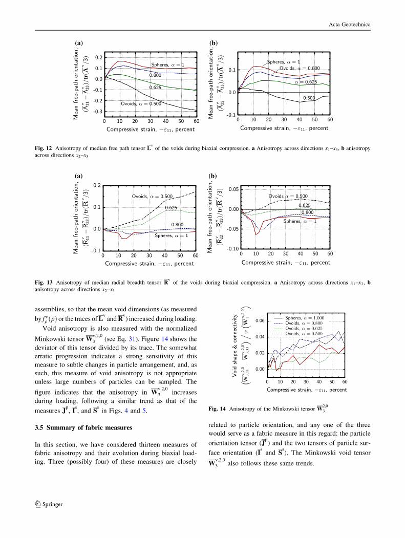
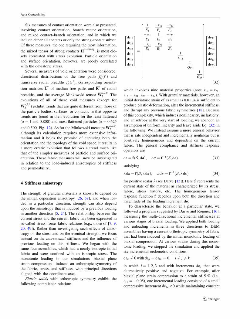
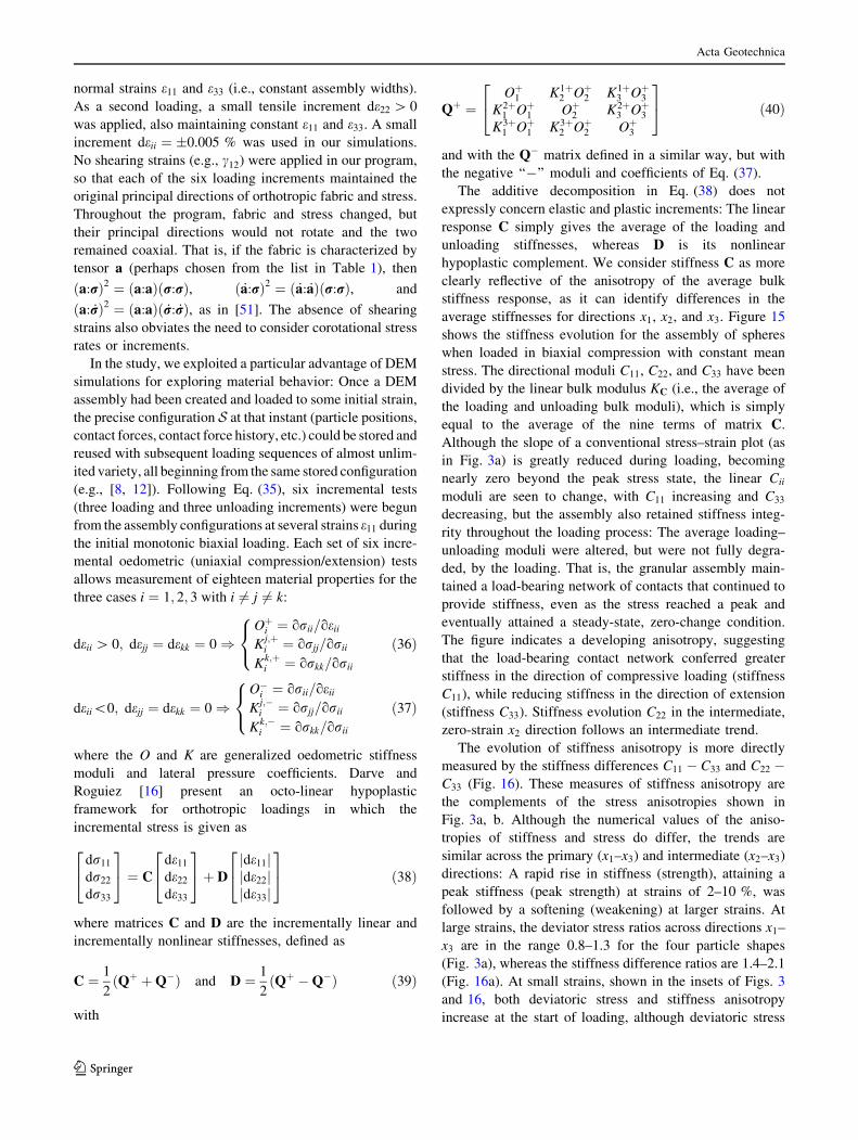
allows measurement of eighteen material properties for the

three cases i ¼ 1; 2; 3 with i 6¼ j 6¼ k:

deii [ 0; dejj ¼ dekk ¼ 0 )Oþ

i ¼ orii=oeiiK

j;þi ¼ orjj=orii

Kk;þi ¼ orkk=orii

8

<

:

ð36Þ

deii\0; dejj ¼ dekk ¼ 0 )O�

i ¼ orii=oeiiK

j;�i ¼ orjj=orii

Kk;�i ¼ orkk=orii

8

<

:

ð37Þ

where the O and K are generalized oedometric stiffness

moduli and lateral pressure coefficients. Darve and

Roguiez [16] present an octo-linear hypoplastic

framework for orthotropic loadings in which the

incremental stress is given as

dr11

dr22

dr33

2

4

3

5 ¼ Cde11

de22

de33

2

4

3

5þ Djde11jjde22jjde33j

2

4

3

5 ð38Þ

where matrices C and D are the incrementally linear and

incrementally nonlinear stiffnesses, defined as

C ¼ 1

2Qþ þQ�ð Þ and D ¼ 1

2Qþ �Q�ð Þ ð39Þ

with

Qþ ¼Oþ

1 K1þ2 Oþ

2 K1þ3 Oþ

3

K2þ1 Oþ

1 Oþ2 K2þ

3 Oþ3

K3þ1 Oþ

1 K3þ2 Oþ

2 Oþ3

2

4

3

5 ð40Þ

and with the Q� matrix defined in a similar way, but with

the negative ‘‘�’’ moduli and coefficients of Eq. (37).

The additive decomposition in Eq. (38) does not

expressly concern elastic and plastic increments: The linear

response C simply gives the average of the loading and

unloading stiffnesses, whereas D is its nonlinear

hypoplastic complement. We consider stiffness C as more

clearly reflective of the anisotropy of the average bulk

stiffness response, as it can identify differences in the

average stiffnesses for directions x1, x2, and x3. Figure 15

shows the stiffness evolution for the assembly of spheres

when loaded in biaxial compression with constant mean

stress. The directional moduli C11, C22, and C33 have been

divided by the linear bulk modulus KC (i.e., the average of

the loading and unloading bulk moduli), which is simply

equal to the average of the nine terms of matrix C.

Although the slope of a conventional stress–strain plot (as

in Fig. 3a) is greatly reduced during loading, becoming

nearly zero beyond the peak stress state, the linear Cii

moduli are seen to change, with C11 increasing and C33

decreasing, but the assembly also retained stiffness integ-

rity throughout the loading process: The average loading–

unloading moduli were altered, but were not fully degra-

ded, by the loading. That is, the granular assembly main-

tained a load-bearing network of contacts that continued to

provide stiffness, even as the stress reached a peak and

eventually attained a steady-state, zero-change condition.

The figure indicates a developing anisotropy, suggesting

that the load-bearing contact network conferred greater

stiffness in the direction of compressive loading (stiffness

C11), while reducing stiffness in the direction of extension

(stiffness C33). Stiffness evolution C22 in the intermediate,

zero-strain x2 direction follows an intermediate trend.

The evolution of stiffness anisotropy is more directly

measured by the stiffness differences C11 � C33 and C22 �C33 (Fig. 16). These measures of stiffness anisotropy are

the complements of the stress anisotropies shown in

Fig. 3a, b. Although the numerical values of the aniso-

tropies of stiffness and stress do differ, the trends are

similar across the primary (x1–x3) and intermediate (x2–x3)

directions: A rapid rise in stiffness (strength), attaining a

peak stiffness (peak strength) at strains of 2–10 %, was

followed by a softening (weakening) at larger strains. At

large strains, the deviator stress ratios across directions x1–

x3 are in the range 0.8–1.3 for the four particle shapes

(Fig. 3a), whereas the stiffness difference ratios are 1.4–2.1

(Fig. 16a). At small strains, shown in the insets of Figs. 3

and 16, both deviatoric stress and stiffness anisotropy

increase at the start of loading, although deviatoric stress

Acta Geotechnica

123

increases with strain more steeply than stiffness anisotropy.

The same trends are apparent across the intermediate

directions x2–x3 (Figs. 3b, 16b).

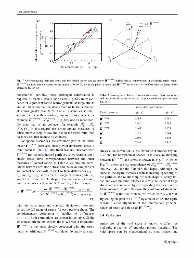
These similarities of stress and stiffness anisotropies

attest to stress and stiffness having a common origin in the

mechanical interactions of particles at their contacts. In

Sect. 3.3, we found that anisotropy of the mixed-fabric

strong-contact tensor, Hc�strong

, correlated most closely

with deviatoric stress. However, we found that the mixed-

fabric contact tensor among all contacts, Hc, most closely

correlates with the anisotropy of the incremental stiffness.

The evolution of this fabric measure is shown in Fig. 6b.

The Pearson coefficient of the stiffness and fabric aniso-

tropies, C11 � C33 and Hc

11 � Hc

33, was an average of 0.985

among the four particle shapes, and the corresponding

average correlation for the x2–x3 anisotropies was 0.981.

Nearly the same correlation was found across all particle

shapes, and ðC11 � C33Þ=KC was consistently about 4.1

times greater than ðHc

11 � Hc

33Þ=trðHc

11 � Hc

33Þ across all

strains and all particle shapes. To summarize, stress is most

closely associated with the fabric of the most heavily

loading contacts (the strong-contact network), whereas

stiffness is most closely correlated with the fabric of all

contacts. Finally, we note that an assembly’s stiffness is not

closely correlated with the orientations of the particle

bodies or of the particle surfaces: Plots of Jp, I

s, and S

s

(Figs. 4, 5) are quite different than those of the stiffness in

Fig. 16.

5 Effective permeability

The particles that form the solid soil skeleton are often

assumed to be impermeable in a timescale important for

most engineering applications. For this case, the hydraulic

properties of the granular assemblies are dictated by the

geometry of the void space among the solid grains. As a

result, the effective permeability tensor of a grain assembly

is isotropic if and only if the microstructural pore geometry

is isotropic. As was seen in Sect. 3.4 for cohesionless

granular media, the pore geometry evolves when subjected

to external loading. While continuum-based numerical

models, such as [65, 67], often employ the size of the void

space to predict permeability, the anisotropy of the effec-

tive permeability is often neglected. Certainly, this treat-

ment may lead to considerable errors in the hydro-

mechanical responses if the eigenvalues of the permeability

tensor are significantly different.

In this study, we analyzed the evolution of permeability

anisotropy by recording the positions of all grains in the

0.20.10

2

1

0

Spheres

C33 /KC

C22 /KC

C11 /KC

Compressive strain, −ε11, percent

Incr

emen

tals

tiffne

sses

,Cii/

KC

6050403020100

4

3

2

1

0

Fig. 15 Evolution of incremental directional stiffnesses of the sphere

assembly. Initial compressive loading is in the x1 direction. Inset plots

detail the small-strain stiffness.

0.20.10

1.0

0.0 α = 0.500α = 0.625α = 0.800Spheres

Compressive strain, −ε11, percent

Incr

emen

tals

tiffne

ssan

isot

ropy

,(C

11−

C33)/

KC

6050403020100

2.5

2.0

1.5

1.0

0.5

0.00.20.10

1.0

0.5

0.0 α = 0.500α = 0.625α = 0.800Spheres

Compressive strain, −ε11, percent

Incr

emen

tals

tiffne

ssan

isot

ropy

,( C

22−

C33)/

KC

6050403020100

1.0

0.5

0.0

(a) (b)

Fig. 16 Anisotropy in the incremental linear stiffness C of four particle shapes: a deviatoric anisotropy across the x1–x3 directions and bintermediate deviatoric anisotropy across the x2–x3 directions. The stiffness deviator is normalized with respect to the average bulk modulus KC.

Inset plots detail the small-strain stiffness

Acta Geotechnica

123

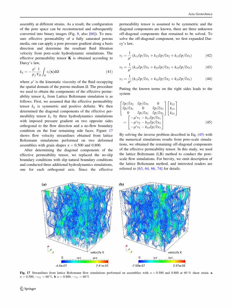
assembly at different strains. As a result, the configuration

of the pore space can be reconstructed and subsequently

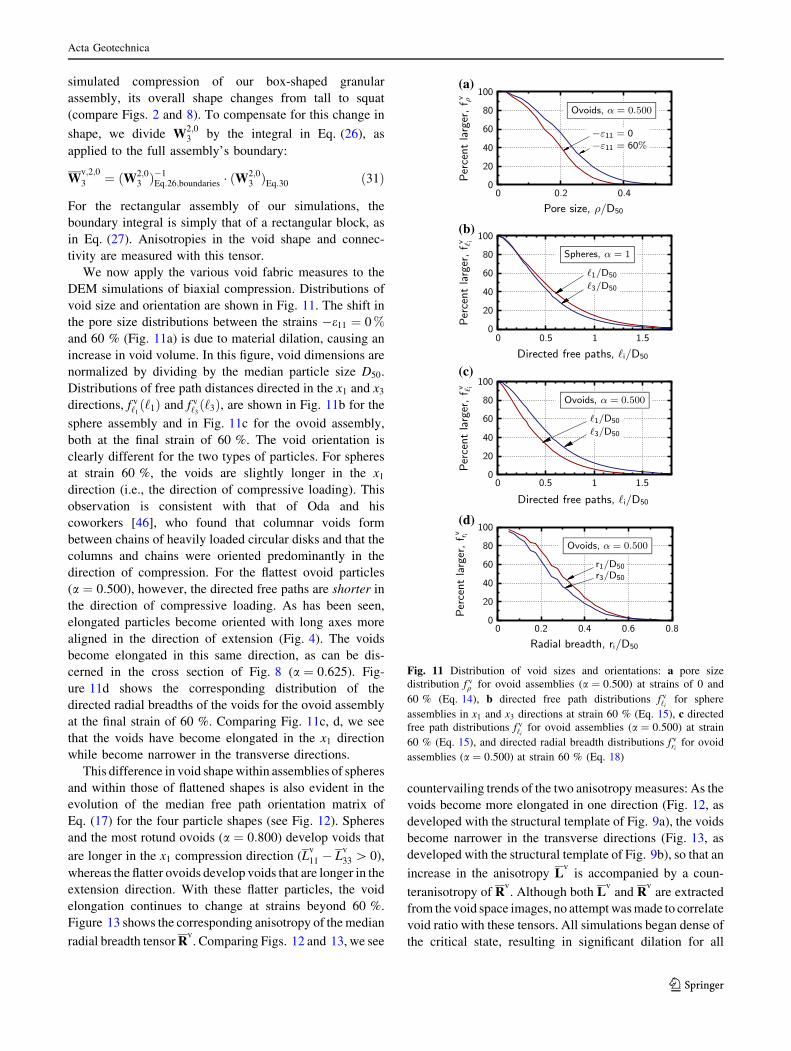
converted into binary images (Fig. 8, also [66]). To mea-

sure effective permeability of a fully saturated porous

media, one can apply a pore pressure gradient along a basis

direction and determine the resultant fluid filtration

velocity from pore-scale hydrodynamic simulations. The

effective permeability tensor K is obtained according to

Darcy’s law,

kij ¼ � lv

p;j

1

VX

Z

XviðxÞdX ð41Þ

where lv is the kinematic viscosity of the fluid occupying

the spatial domain of the porous medium X. The procedure

we used to obtain the components of the effective perme-

ability tensor kij from Lattice Boltzmann simulation is as

follows. First, we assumed that the effective permeability

tensor kij is symmetric and positive definite. We then

determined the diagonal components of the effective per-

meability tensor kii by three hydrodynamics simulations

with imposed pressure gradient on two opposite sides

orthogonal to the flow direction and a no-flow boundary

condition on the four remaining side faces. Figure 17

shows flow velocity streamlines obtained from lattice

Boltzmann simulations performed on two deformed

assemblies with grain shapes a ¼ 0:500 and 0.800.

After determining the diagonal components of the

effective permeability tensor, we replaced the no-slip

boundary conditions with slip natural boundary conditions

and conducted three additional hydrodynamics simulations,

one for each orthogonal axis. Since the effective

permeability tensor is assumed to be symmetric and the

diagonal components are known, there are three unknown

off-diagonal components that remained to be solved. To

solve the off-diagonal component, we first expanded Dar-

cy’s law,

v1 ¼ 1

lvðk11op=ox1 þ k12op=ox2 þ k13op=ox3Þ ð42Þ

v2 ¼ 1

lvðk12op=ox1 þ k22op=ox2 þ k23op=ox3Þ ð43Þ

v3 ¼ 1

lvðk13op=ox1 þ k32op=ox2 þ k33op=ox3Þ ð44Þ

Putting the known terms on the right sides leads to the

system

op=ox2 op=ox3 0

op=ox1 0 op=ox3

0 op=ox1 op=ox2

2

4

3

5

k12

k13

k23

2

4

3

5

¼�lvv1 � k11op=ox1

�lvv2 � k22op=ox2

�lvv3 � k33op=ox3

2

4

3

5 ð45Þ

By solving the inverse problem described in Eq. (45) with

the numerical simulations results from pore-scale simula-

tions, we obtained the remaining off-diagonal components

of the effective permeability tensor. In this study, we used

the lattice Boltzmann (LB) method to conduct the pore-

scale flow simulations. For brevity, we omit description of

the lattice Boltzmann method, and interested readers are

referred to [63, 64, 66, 74] for details.

Fig. 17 Streamlines from lattice Boltzmann flow simulations performed on assemblies with a ¼ 0:500 and 0.800 at 60 % shear strain. aa ¼ 0:500;��11 ¼ 60%, b a ¼ 0:800;��11 ¼ 60%

Acta Geotechnica

123

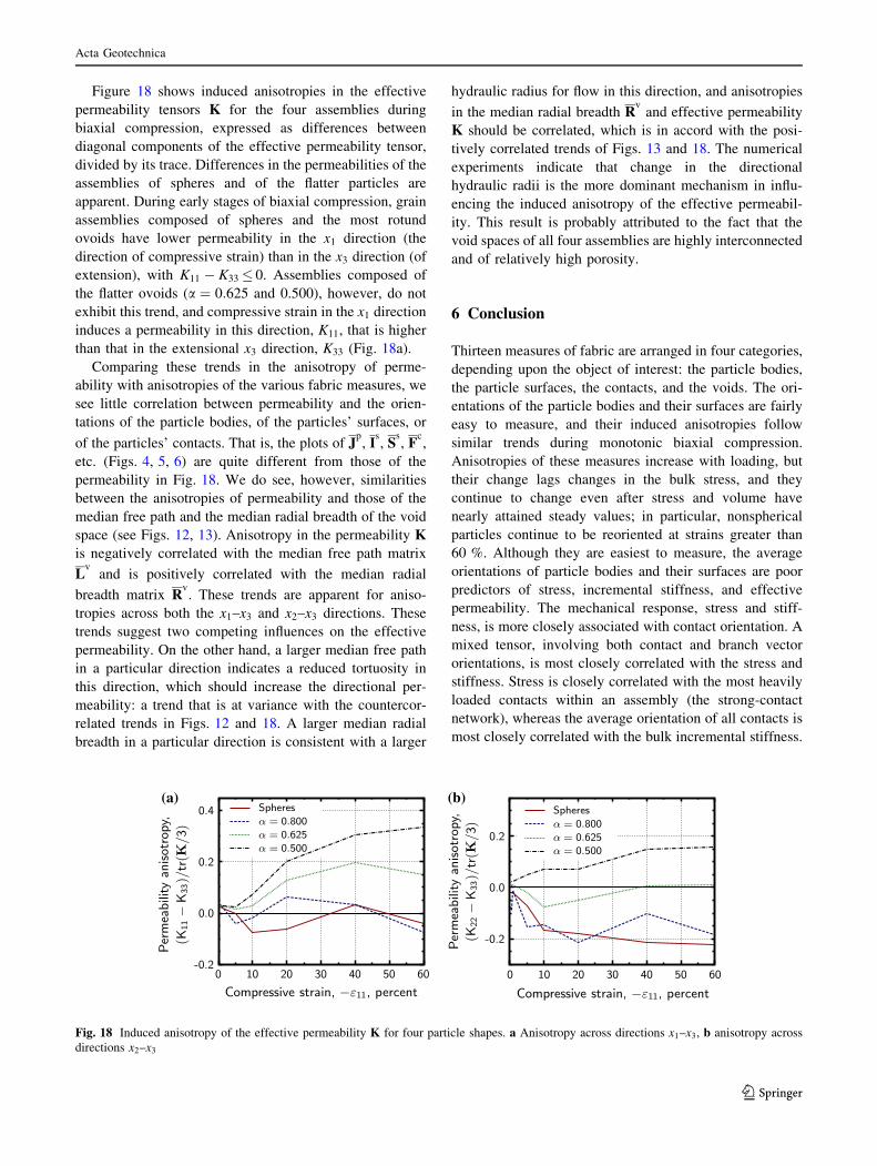
Figure 18 shows induced anisotropies in the effective

permeability tensors K for the four assemblies during

biaxial compression, expressed as differences between

diagonal components of the effective permeability tensor,

divided by its trace. Differences in the permeabilities of the

assemblies of spheres and of the flatter particles are

apparent. During early stages of biaxial compression, grain

assemblies composed of spheres and the most rotund

ovoids have lower permeability in the x1 direction (the

direction of compressive strain) than in the x3 direction (of

extension), with K11 � K33 0. Assemblies composed of

the flatter ovoids (a ¼ 0:625 and 0.500), however, do not

exhibit this trend, and compressive strain in the x1 direction

induces a permeability in this direction, K11, that is higher

than that in the extensional x3 direction, K33 (Fig. 18a).

Comparing these trends in the anisotropy of perme-

ability with anisotropies of the various fabric measures, we

see little correlation between permeability and the orien-

tations of the particle bodies, of the particles’ surfaces, or

of the particles’ contacts. That is, the plots of Jp, I

s, S

s, F

c,

etc. (Figs. 4, 5, 6) are quite different from those of the

permeability in Fig. 18. We do see, however, similarities

between the anisotropies of permeability and those of the

median free path and the median radial breadth of the void

space (see Figs. 12, 13). Anisotropy in the permeability K

is negatively correlated with the median free path matrix

Lv

and is positively correlated with the median radial

breadth matrix Rv. These trends are apparent for aniso-

tropies across both the x1–x3 and x2–x3 directions. These

trends suggest two competing influences on the effective

permeability. On the other hand, a larger median free path

in a particular direction indicates a reduced tortuosity in

this direction, which should increase the directional per-

meability: a trend that is at variance with the countercor-

related trends in Figs. 12 and 18. A larger median radial

breadth in a particular direction is consistent with a larger

hydraulic radius for flow in this direction, and anisotropies

in the median radial breadth Rv

and effective permeability

K should be correlated, which is in accord with the posi-

tively correlated trends of Figs. 13 and 18. The numerical

experiments indicate that change in the directional

hydraulic radii is the more dominant mechanism in influ-

encing the induced anisotropy of the effective permeabil-

ity. This result is probably attributed to the fact that the

void spaces of all four assemblies are highly interconnected

and of relatively high porosity.

6 Conclusion

Thirteen measures of fabric are arranged in four categories,

depending upon the object of interest: the particle bodies,

the particle surfaces, the contacts, and the voids. The ori-

entations of the particle bodies and their surfaces are fairly

easy to measure, and their induced anisotropies follow

similar trends during monotonic biaxial compression.

Anisotropies of these measures increase with loading, but

their change lags changes in the bulk stress, and they

continue to change even after stress and volume have

nearly attained steady values; in particular, nonspherical

particles continue to be reoriented at strains greater than

60 %. Although they are easiest to measure, the average

orientations of particle bodies and their surfaces are poor

predictors of stress, incremental stiffness, and effective

permeability. The mechanical response, stress and stiff-

ness, is more closely associated with contact orientation. A

mixed tensor, involving both contact and branch vector

orientations, is most closely correlated with the stress and

stiffness. Stress is closely correlated with the most heavily

loaded contacts within an assembly (the strong-contact

network), whereas the average orientation of all contacts is

most closely correlated with the bulk incremental stiffness.

α = 0.500α = 0.625α = 0.800Spheres

Compressive strain, −ε11, percent

Per

mea

bilit

yan

isot

ropy

,(K

11−

K33)/

tr(K

/3)

6050403020100

0.4

0.2

0.0

-0.2

α = 0.500α = 0.625α = 0.800Spheres

Compressive strain, −ε11, percent

Per

mea

bilit

yan

isot

ropy

,(K

22−

K33) /

tr(K

/3)

6050403020100

0.2

0.0

-0.2

(a) (b)

Fig. 18 Induced anisotropy of the effective permeability K for four particle shapes. a Anisotropy across directions x1–x3, b anisotropy across

directions x2–x3

Acta Geotechnica

123

In short, tensor Hc�strong is the preferred fabric measure for

stress, and tensor Hc is the preferred fabric measure for

incremental stiffness. Two principal measures of pore

anisotropy were investigated in regard to the effective

permeability: one related to the directional median free

path (a countermeasure of tortuosity) and the other related

to the directional median radial breadth (a measure of

hydraulic radius). The preferred measure for effective

permeability is the matrix of the median radial breadths of

the void space, Rv, as it correlates closely with

permeability.

Acknowledgments This research was partially supported by the

Earth Materials and Processes program at the US Army Research

Office under Grant contract W911NF-14-1-0658 and the Provosts

Grants Program for Junior Faculty who Contribute to the Diversity

Goals of the University at Columbia University. The Tesla K40 used

for the lattice Boltzmann simulations was donated by the NVIDIA

Corporation. These supports are gratefully acknowledged.

References

1. Adler PM (1992) Porous media: geometry and transports. But-

terworth-Heinemann, Boston

2. Ando E, Viggiani G, Hall SA, Desrues J (2013) Experimental

micro-mechanics of granular media studied by X-ray tomogra-

phy: recent results and challenges. Geotech Lett 3:142–146

3. Antony SJ, Kuhn MR (2004) Influence of particle shape on

granular contact signatures and shear strength: new insights from

simulations. Int J Solids Struct Granul Mech 41(21):5863–5870

4. Arns CH, Bauget F, Limaye A, Arthur Sakellariou TJ, Senden

APS, Sok RM, Pinczewski WV, Bakke S, Berge LI et al (2005)

Pore-scale characterization of carbonates using X-ray microto-

mography. SPE J Richardson 10(4):475

5. Arthur JRF, Chua KS, Dunstan T (1977) Induced anisotropy in a

sand. Geotechnique 27(1):13–30

6. Arthur JRF, Menzies BK (1972) Inherent anisotropy in a sand.

Geotechnique 22(1):115–128

7. Azema E, Radjaı F, Peyroux R, Saussine G (2007) Force trans-

mission in a packing of pentagonal particles. Phys Rev E 76:011301

8. Bardet JP (1994) Numerical simulations of the incremental

responses of idealized granular materials. Int J Plast

10(8):879–908

9. Bathurst RJ, Rothenburg L (1990) Observations on stress–force–

fabric relationships in idealized granular materials. Mech Mater

9:65–80 fabric, DEM, circles

10. Bear J (2013) Dynamics of fluids in porous media. Courier

Corporation, Chelmsford

11. Calvetti F, Combe G, Lanier J (1997) Experimental microme-

chanical analysis of a 2D granular material: relation between

structure evolution and loading path. Mech Cohesive Frict Mater

2(2):121–163

12. Calvetti F, Viggiani G, Tamagnini C (2003) A numerical inves-

tigation of the incremental behavior of granular soils. Rivista

Italiana di Geotecnica 3:11–29

13. Chapuis RP, Gill DE, Baass K (1989) Laboratory permeability

tests on sand: influence of the compaction method on anisotropy.

Can Geotech J 26(4):614–622

14. Chen Y-C, Hung H-Y (1991) Evolution of shear modulus and

fabric during shearing deformation. Soils Found 31(4):148–160

15. Darve F (1990) The expression of rheological laws in incremental

form and the main classes of constitutive equations. In: Darve F

(ed) Geomaterials: constitutive equations and modelling. Else-

vier, London, pp 123–147

16. Darve F, Roguiez X (1999) Constitutive relations for soils: new

challenges. Rivista Italiana di Geotecnica 4:9–35

17. DeHoff RT, Aigeltinger EH, Craig KR (1972) Experimental

determination of the topological properties of three-dimensional

microstructures. J Microsc 95(1):69–91

18. Dobry R, Ladd RS, Yokel FY, Chung RM, Powell D (1982)

Prediction of pore water pressure buildup and liquefaction of

sands during earthquakes by the cyclic strain method. NBS

Building Science Series 138, Natl. Bureau of Standards

19. Fredrich JT, Menendez B, Wong TF (1995) Imaging the pore

structure of geomaterials. Science 268(5208):276–279

20. Guo N, Zhao J (2013) The signature of shear-induced anisotropy

in granular media. Comput Geotech 47:1–15

21. Hall SA, Muir Wood D, Ibraim E, Viggiani G (2010) Localised

deformation patterning in 2D granular materials revealed by

digital image correlation. Granul Matter 12(1):1–14

22. Hilpert M, Glantz R, Miller CT (2003) Calibration of a pore-

network model by a pore-morphological analysis. Transp Porous

Media 51(3):267–285

23. Hoque E, Tatsuoka F (1998) Anisotropy in elastic deformation of

granular materials. Soils Found 38(1):163–179

24. Ishibashi I, Chen Y-C, Chen M-T (1991) Anisotropic behavior of

Ottawa sand in comparison with glass spheres. Soils Found

31(1):145–155

25. Kanatani K (1988) Stereological estimation of microstructures in

materials. In: Satake M, Jenkins JT (eds) Micromechanics of

granular materials. Elsevier, Amsterdam, pp 1–10

26. Konishi J, Oda M, Nemat-Nasser S (1982) Inherent anisotropy

and shear strength of assembly of oval cross-sectional rods. In:

Vermeer PA, Luger HJ (eds) Deformation and failure of granular

materials. A.A. Balkema Pub, Rotterdam, pp 403–412

27. Koutsourelakis PS, Deodatis G (2006) Simulation of multidi-

mensional binary random fields with application to modeling of

two-phase random media. J Eng Mech 132(6):619–631

28. Kruyt NP (2012) Micromechanical study of fabric evolution in

quasi-static deformation of granular materials. Mech Mater

44:120–129

29. Kruyt NP, Rothenburg L (2009) Plasticity of granular materials: a

structural-mechanics view. In: AIP conference proceedings vol

1145, p 1073

30. Kuhn MR (2002) OVAL and OVALPLOT: programs for ana-

lyzing dense particle assemblies with the Discrete Element

Method. http://faculty.up.edu/kuhn/oval/oval.html

31. Kuhn MR (2003) Smooth convex three-dimensional particle for

the discrete element method. J Eng Mech 129(5):539–547

32. Kuhn MR (2010) Micro-mechanics of fabric and failure in

granular materials. Mech Mater 42(9):827–840

33. Kuhn MR, Renken H, Mixsell A, Kramer S (2014) Investigation

of cyclic liquefaction with discrete element simulations.

J Geotech Geoenviron Eng 140(12):04014075

34. Kuo C-Y, Frost JD, Chameau J-LA (1998) Image analysis

determination of stereology based fabric tensors. Geotechnique

48(4):515–525

35. Kwiecien MJ, Macdonald IF, Dullien FAL (1990) Three-di-

mensional reconstruction of porous media from serial section

data. J Microsc 159(3):343–359

36. Li X, Dafalias Y (2002) Constitutive modeling of inherently

anisotropic sand behavior. J Geotech Geoenviron Eng

128(10):868–880

37. Liang Z, Ioannidis MA, Chatzis I (2000) Geometric and topo-

logical analysis of three-dimensional porous media: pore space

Acta Geotechnica

123

partitioning based on morphological skeletonization. J Colloid

Interface Sci 221(1):13–24

38. Lindquist WB, Lee S-M, Coker DA, Jones KW, Spanne P (1996)

Medial axis analysis of void structure in three-dimensional

tomographic images of porous media. J Geophys Res Solid Earth

(1978–2012) 101(B4):8297–8310

39. Magoariec H, Danescu A, Cambou B (2008) Nonlocal orienta-

tional distribution of contact forces in granular samples con-

taining elongated particles. Acta Geotech 3(1):49–60

40. Majmudar TS, Bhehringer RP (2005) Contact force measure-

ments and stress-induced anisotropy in granular materials. Nature

435(1079):1079–1082

41. Michielsen K, De Raedt H (2001) Integral-geometry morpho-

logical image analysis. Phys Rep 347(6):461–538

42. Mitchell JK, Soga K (2005) Fundamentals of soil behavior, 3rd

edn. Wiley, New York

43. Ng T-T (2001) Fabric evolution of ellipsoidal arrays with dif-

ferent particle shapes. J Eng Mech 127(10):994–999

44. Oda M (1972) Initial fabrics and their relations to mechanical

properties of granular material. Soils Found 12(1):17–36

45. Oda M (1972) The mechanism of fabric changes during com-

pressional deformation of sand. Soils Found 12(2):1–18

46. Oda M, Kazama H (1998) Microstructure of shear bands and its

relation to the mechanisms of dilatancy and failure of dense

granular soils. Geotechnique 48(4):465–481

47. Oda M, Nemat-Nasser S, Konishi J (1985) Stress-induced ani-

sotropy in granular masses. Soils Found 25(3):85–97

48. Ouadfel H, Rothenburg L (1999) An algorithm for detecting

inter-ellipsoid contacts. Comput Geotech 24(4):245–263

49. Ouadfel H, Rothenburg L (2001) Stress–force–fabric relationship

for assemblies of ellipsoids. Mech Mater 33(4):201–221

50. Pena AA, Garcıa-Rojo R, Herrmann HJ (2007) Influence of

particle shape on sheared dense granular media. Granul Matter

9:279–291

51. Pietruszczak S, Mroz Z (2001) On failure criteria for anisotropic

cohesive–frictional materials. Int J Numer Anal Methods Geo-

mech 25(5):509–524

52. Prasad PB, Jernot JP (1991) Topological description of the den-

sification of a granular medium. J Microsc 163(2):211–220

53. Radjai F, Wolf DE, Jean M, Moreau J-J (1998) Bimodal character

of stress transmission in granular packings. Phys Rev Lett

80(1):61–64

54. Reeves PC, Celia MA (1996) A functional relationship between

capillary pressure, saturation, and interfacial area as revealed by a

pore-scale network model. Water Resour Res 32(8):2345–2358

55. Rothenburg L, Bathurst RJ (1989) Analytical study of induced

anisotropy in idealized granular materials. Geotechnique

39(4):601–614

56. Rothenburg L, Bathurst RJ (1992) Micromechanical features of

granular assemblies with planar elliptical particles. Geotechnique

42(1):79–95

57. Santamarina JC, Cascante G (1996) Stress anisotropy and wave

propagation: a micromechanical view. Can Geotech J

33(5):770–782

58. Satake M (1982) Fabric tensor in granular materials. In: Vermeer

PA, Luger HJ (eds) Proceedings of IUTAM symposium on

deformation and failure of granular materials. A.A. Balkema,

Rotterdam, pp 63–68

59. Schroder-Turk GE, Mickel W, Kapfer SC, Klatt MA, Schaller

FM, Hoffmann MJF, Kleppmann N, Armstrong P, Inayat A, Hug

D, Reichelsdorfer M, Peukert W, Schwieger W, Mecke K (2011)

Minkowski tensor shape analysis of cellular, granular and porous

structures. Adv Mater 23(22–23):2535–2553

60. Schroder-Turk GE, Mickel W, Kapfer SC, Schaller FM, Brei-

denbach B, Hug D, Mecke K (2010) Minkowski tensors of ani-

sotropic spatial structure. arXiv preprint arXiv:1009.2340

61. Serra J (1982) Image analysis and mathematical morphology.

Academic Press, London

62. Sun WC (2015) A stabilized finite element formulation for

monolithic thermo-hydro-mechanical simulations at finite strain.

Int J Numer Methods Eng. doi:10.1002/nme.4910

63. Sun WC, Andrade JE, Rudnicki JW (2011) Multiscale method for

characterization of porous microstructures and their impact on

macroscopic effective permeability. Int J Numer Meth Eng

88(12):1260–1279

64. Sun WC, Andrade JE, Rudnicki JW, Eichhubl P (2011) Con-

necting microstructural attributes and permeability from 3D

tomographic images of in situ shear-enhanced compaction bands

using multiscale computations. Geophys Res Lett 38(10):L10302

65. Sun WC, Chen Q, Ostien JT (2014) Modeling the hydro-me-

chanical responses of strip and circular punch loadings on water-

saturated collapsible geomaterials. Acta Geotech 9(5):903–934

66. Sun WC, Kuhn MR, Rudnicki JW (2013) A multiscale DEM-

LBM analysis on permeability evolutions inside a dilatant shear

band. Acta Geotech 8(5):465–480

67. Sun WC, Ostien JT, Salinger AG (2013) A stabilized assumed

deformation gradient finite element formulation for strongly

coupled poromechanical simulations at finite strain. Int J Numer

Anal Meth Geomech 37(16):2755–2788

68. Tatsuoka F, Nakamura S, Huang C-C, Tani K (1990) Strength

anisotropy and shear band direction in plane strain tests of sand.

Soils Found 30(1):35–54

69. Thornton C (1990) induced anisotropy and energy dissipation in

particulate material—results from computer-simulated experi-

ments. In: Boehler JP (ed) Yielding, damage, and failure of ani-

sotropic solids. Mechanical Engineering Pub, London, pp 113–130

70. Thornton C, Antony SJ (1998) Quasi-static deformation of par-

ticulate media. Philos Trans R Soc Lond A 356(1747):2763–2782

71. Thornton C, Zhang L (2010) On the evolution of stress and

microstructure during general 3D deviatoric straining of granular

media. Geotechnique 60(5):333–341

72. Vogel HJ (1997) Morphological determination of pore connec-

tivity as a function of pore size using serial sections. Eur J Soil

Sci 48(3):365–377

73. Wang Y, Mok C (2008) Mechanisms of small-strain shear-

modulus anisotropy in soils. J Geotech Geoenviron Eng

134(10):1516–1530

74. White JA, Borja RI, Fredrich JT (2006) Calculating the effective

permeability of sandstone with multiscale lattice Boltzmann/

finite element simulations. Acta Geotech 1(4):195–209

75. Wong RCK (2003) A model for strain-induced permeability

anisotropy in deformable granular media. Can Geotech J

40(1):95–106

76. Zaretskiy Y, Geiger S, Sorbie K, Forster M (2010) Efficient flow

and transport simulations in reconstructed 3D pore geometries.

Adv Water Resour 33(12):1508–1516

77. Zhao J, Guo N (2013) A new definition on critical state of

granular media accounting for fabric anisotropy. AIP Conf Proc

1542:229–232

78. Zhu W, Montesi LGJ, Wong T (2007) A probabilistic damage

model of stress-induced permeability anisotropy during cata-

clastic flow. J Geophys Res 112(B10):B10207

Acta Geotechnica

123