Stress testing a retail loan portfolio: an error ... · The Journal of Risk Model Validation...

The Journal of Risk Model Validation (3–25) Volume 6/Number 1, Spring 2012

Stress testing a retail loan portfolio:an error correction model approach

Steeve AssouanGroupe de Recherche Operationnelle, Credit Agricole S.A.,12 Place des Etats-Unis, 92127 Montrouge, France;email: [email protected]

The use of stress testing for risk monitoring has increased considerably over thelast decade. Stress testing – a simulation technique used to assess the strength of aportfolio or a financial institution under unusual economic conditions – emergedas a powerful tool that was originally used in market risk. Its use has subsequentlybeen extended into credit risk. To stress test a credit risk portfolio, practitionersfocus on the key parameters that allow the risk of a credit portfolio to be assessed.These parameters, also known as Basel II parameters, are probability of default,loss given default, exposure at default and asset correlation. In this paper, usinga time series approach (specifically, an error correction model), we focus on theprobability of default parameter that is related to macroeconomic factors. Suchan approach involves dealing with the nonstationarity of economic time seriesand cointegration issues. Hence, when the model is estimated, the probabilityof default can be simulated by measuring the effects of macroeconomic shocksapplied to the model. In turn, these probabilities of default can be used to measurethe impact on the probability of default under a given macroeconomic scenario,and then to improve the credit risk monitoring. The results of our study suggest thaterror correction models are well-suited to macroeconomic stress testing. Indeed,the fitting of the historical probability of default and the results under the stressscenarios considered here are satisfactory.

1 INTRODUCTION

The recent economic and financial crisis led to the collapse of many firms, andmacroeconomic uncertainty and lower household creditworthiness have reinforcedthe importance of credit risk, the central risk faced by banks (more than 80% of a

The views expressed in this paper are solely the responsibility of the author and should not beinterpreted as reflecting the opinions or official positions of Crédit Agricole S.A. I am grateful toSophie Lavaud for her fruitful contribution, Vincent Lehérissé for his useful comments, and SylvainPoëta, who gave me the opportunity to work on this issue. The usual disclaimer nonetheless applies,and any errors are my own.

3

4 S. Assouan

bank’s overall risk). Supervisors have therefore promoted the setting up of a stress-testing process, and central banks took the lead in stress-test research. In addition,the need for an intensification of credit risk monitoring tools has enhanced the roleplayed by macroeconomic stress testing.

To assess the credit exposure and potential losses that they face, banks have toestimate a set of parameters (probability of default (PD), loss given default (LGD)and exposure at default) that are required to calculate regulatory capital in the Baselframework. Practitioners commonly begin by estimating the PD parameter, which isthe basic input when evaluating a portfolio’s credit risk especially during recessions.Therefore, risk managers and regulators are interested in the prediction of PD (andpotential losses) under a given macroeconomic scenario. They wish to improve themonitoring of their portfolio credit risk through stress testing.

Two main approaches have been provided in the literature (see Sorge (2004)) formacroeconomic stress testing: the piecewise approach and the integrated approach.Risk managers adopting the integrated approach combine the analysis of multiplerisk factors into a single portfolio loss distribution, while the piecewise approachinvolves forecasting models of individual financial soundness indicators. We adoptthe piecewise approach, which allows us to design a broader stress scenario than ispossible in the integrated approach. In addition, this approach is more intuitive andhas a lower computational burden.

The literature has produced a lot of models for macroeconomic stress testing inthe piecewise framework. The most common method used for performing macro-economic stress testing on a credit portfolio is a time series approach, particularly thevector autoregressive (VAR) model. These studies have been made for a corporateloans portfolio (see Avouyi-Dovis et al (2009)) and for a whole banking or financialsystem (Hoggarth et al (2005)), but retail portfolios have not received as much atten-tion. Bucay and Rosen (2001) develop a methodology for measuring the credit risk ofa retail portfolio (which can be used to perform macroeconomic stress testing) usingan integrated approach. Since we adopt a piecewise approach, the distinctive featureof this paper is that it applies statistical methods that are usually used for a corporateportfolio to a retail portfolio.

A VAR model is inappropriate for our study since, in a VAR model, all the vari-ables used (macroeconomic variables and a portfolio’s default rates) are consideredendogenous. From our point of view, there is no causal relationship between the PDof a consumer loan portfolio and France’s gross domestic product (GDP) or three-month interest rate. So we choose to consider a model based on a time series approachwhere macroeconomic factors are exogenous. Note that Rösch and Scheule (2007)use a credit risk model derived from Merton’s (1974) model to carry out a stress teston credit risk parameters with an application to retail loan portfolios, but they do notuse a time series approach. In this paper we relate the PD of two retail loan portfolios

The Journal of Risk Model Validation Volume 6/Number 1, Spring 2012

Stress testing a retail loan portfolio 5

to key macroeconomic factors using a time series approach. Macroeconomic-basedmodels are motivated by an a priori link between the PD and the macroeconomicenvironment. It is well-known that PD increases during a recession.

This paper is organized as follows. In Section 2 we discuss the use of stress testingas a risk management tool. Section 3 introduces the model setup and some intuitionsare given about the mechanism of an error correction model (ECM). We then explainthe estimation procedure. Section 4 describes the data set. In Section 5 we performa macroeconomic stress test under two scenarios and discuss the results. Section 6concludes.

2 STRESS TESTING AS A RISK MANAGEMENT TOOL

According to the Bank for International Settlements, a stress test is described as “theevaluation of the financial position of a bank under a severe but plausible scenario toassist in decision making within the bank” (Basel Committee on Banking Supervision(2009)). Stress testing has become an important risk management tool used by banks aspart of their internal risk management process and promoted by supervisors throughthe Basel II capital adequacy framework. Moreover, stress testing provides bankswith another tool with which to supplement other risk management approaches andmeasures. Again following the Bank for International Settlements definition, stresstesting plays a particularly important role in

� providing forward-looking assessments of risk,

� overcoming limitations of models and historical data,

� supporting internal and external communication,

� feeding into capital and liquidity planning procedures,

� informing the setting of banks’ risk tolerance,

� easing the development of risk mitigation or contingency plans across a rangeof stressed conditions.

Since stress testing is an essential element of the Basel II framework, practitioners(risk and business managers) and regulators are interested in quantitative methods forassessing the potential risk of their bank or specific loans portfolio under a hypotheticalbut plausible stress scenario. Although the use of stress testing by banks appears tohave been growing prior to the crisis, a 2005 Bank for International Settlements studyshowed that the focus at that time was primarily on applications to market risk: 80% ofthe tests were related to market risk. However, since the crisis, more attention has beenpaid to the integration of other types of risk, especially the credit risk portfolio. Stress

Research Paper www.journalofriskmodelvalidation.com

6 S. Assouan

testing appears to be useful in a broad variety of contexts, from regulatory reportingand risk management to newer uses such as strategic planning (assessing banks’ riskappetite and determining which business segments to grow or stem), improvement ofbanks’ risk management (by anticipating future risk level) or banks’ budget planning.

Stress tests can be divided into two categories: scenario tests and sensitivity tests.In the first case, the stress scenarios are based on a portfolio-driven approach oran event-driven approach. Event-driven scenarios, which are generally requested bysenior management and motivated by recent news, are based on plausible events andhow these events might affect the relevant risk factors for a bank or a given portfolio.In contrast, in the portfolio-driven approach, risk managers discuss and identify riskdrivers of a given portfolio and then design plausible scenarios under which thesefactors are stressed. For example, if risk managers identify unemployment rate as theirmain risk factor, stress tests will be designed around changes in the unemploymentrate.

Moreover, under each approach, events can be categorized as either historical orhypothetical scenarios. Historical scenarios are based on historical data and rely ona crisis experienced in the past, while hypothetical scenarios are based on plausiblescenarios that have not yet happened.

In sensitivity tests, risk factors are moved instantaneously by a unit amount and thesource of the shock is not identified. Moreover, the time horizon for sensitivity testsis generally shorter in comparison with scenarios.

In this paper we perform a scenario stress test for a retail loan portfolio and usehypothetical scenarios instead of historical ones.

3 A MACROECONOMIC CREDIT RISK MODEL

Wilson (1997a,b) develops a credit risk model linking macroeconomic factors andcorporate sector default rates. The idea was to model the relationship between defaultrates and macroeconomic factors and, when a model is fitted, to simulate the evolutionof default rates over time by applying a stress scenario to the model. The simulateddefault rates in turn make it possible to obtain estimates of default rates for a definedcredit portfolio under a given stress scenario.

Our approach, derived from Wilson’s approach, considers a one-year observed PDinstead of the default rates. In the following sections we use PD for the observedprobability of default.

The PD is modeled by a logistic functional form:

PDt D1

1C exp.�yt /, yt D ln

�PDt

1 � PDt

�(3.1)



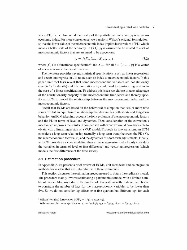
where PDt is the observed default rates of the portfolio at time t and yt is a macro-economic index. For more convenience, we transform Wilson’s original formulation1

so that the lower value of the macroeconomic index implies lower values of PD, whichmeans a better state of the economy. In (3.1), yt is assumed to be related to a set ofmacroeconomic factors that are assumed to be exogenous:

yt D f .Xt ; Xt�1; Xt�2; : : : / (3.2)

where f .�/ is a functional specification2 and Xt�i for all i 2 f0; : : : ; pg is a vectorof macroeconomic factors at time t � i .

The literature provides several statistical specifications, such as linear regressionsand vector autoregressions, to relate such an index to macroeconomic factors. In thispaper, unit root tests reveal that some macroeconomic variables are not stationary(see (A.2) for details) and this nonstationarity could lead to spurious regressions inthe case of a linear specification. To address this issue we choose to take advantageof the nonstationarity property of the macroeconomic time series and thereby spec-ify an ECM to model the relationship between the macroeconomic index and themacroeconomic factors.

Recall that ECMs are based on the behavioral assumption that two or more timeseries exhibit an equilibrium relationship that determines both short- and long-termbehavior.An ECM takes into account the joint evolution of the macroeconomic factorsand the PD in terms of level and dynamics. Then consideration of the correction’smechanism improves the results in comparison with what we would have been able toobtain with a linear regression or a VAR model. Through its two equations, an ECMconsiders a long-term relationship (actually a long-term trend) between the PD (Y ),the macroeconomic factors (X ) and the dynamics of short-term adjustments. Finally,an ECM provides a richer modeling than a linear regression (which only considersthe variables in terms of level or first difference) and vector autoregression (whichmodels the first difference of the time series).

3.1 Estimation procedure

In Appendix A we present a brief review of ECMs, unit roots tests and cointegrationmethods for readers that are unfamiliar with these techniques.

This section discusses the estimation procedure used to obtain the credit risk model.The procedure mainly involves estimating a parsimonious model with a limited num-ber of factors. Moreover, due to the number of observations in the data set, we chooseto constrain the number of lags for the macroeconomic variables to be lower thanfive. So we do not consider lag effects over five quarters but different lags for each

1 Wilson’s original formulation is PDt D 1=.1C exp.yt //.2 Wilson chose the linear specification yt D ˇ0 C ˇ1x1;t C ˇ2x2;t C � � � C ˇnxn;t C "t .


8 S. Assouan

macroeconomic variable have been tested. Moreover, in line with the economists ofCrédit Agricole, we set up a priori signs for each macroeconomic factor with respectto economic theory: the interpretation of our model is therefore ensured. Finally,in order to be included in a model, each macroeconomic variable has to fulfill twoconditions:

(1) its coefficients must be statistically significant and improve the overall model’sperformance;

(2) its coefficients must be consistent with economic theory.

Two methods exist in the literature for estimating the ECM: the one-step procedureand the two-step procedure.

Assuming Equation (A.1), the one-step method reduces the estimation procedureto the estimation of the following linear regression:

�Yt D �Yt�1 � .� C �˛/Xt�1 C �Xt C �Zt C vt (3.3)

This one-step procedure, which was popularized in economics by Davidson et al(1978), is quite easy to perform and requires weak exogeneity as an appropriateassumption. The validity of this assumption affects the estimation’s result and couldlead to (3.3) being both biased and inefficient and, therefore, the t -tests based on themodel’s parameter would be highly misleading.

The two-step procedure, introduced by Engle and Granger (1987), proceeds as fol-lows. In the first step, we assume thatYt andXt (a vector of macroeconomic variables)are integrated of the same order and thatZt is a vector of stationary component. Hav-ing defined the integration order and potential cointegrated variables, the long-termrelationship is estimated as the linear regression of Yt on Xt :

Yt D ˛Xt C "t (3.4)

A more complex lag structure could be tested forXt . If "t , the long-term relationship’sresidual, is stationary, Yt and Xt are said to be cointegrated. Thus, the second stepcould be performed. Note that, ifXt and Yt are cointegrated, an ordinary least-squares(OLS) regression yields a superconsistent estimator of ˛, since rate convergenceequals T rather than

pT , as in the standard context.

At this step, �Yt is regressed on "t�1 and �Xt . Additional stationary variables oralternative lags (and deterministic terms) may be included as well:

�Yt D � O"t�1„ƒ‚…Yt�1� OXt�1

C ��Xt C �Zt C �t (3.5)

Moreover, it is known that, in the presence of unit roots in time series and cointe-grating regression without serially correlated errors, the two-step procedure performs



well. However, we cannot perform any test on the long-term parameters since the lim-iting distribution of ˛ parameters are nonnormal and nonstandard. Then the two-stepprocedure implies that any mistake introduced in the first step is carried forward inthe second step.

Note that the Engle and Granger two-step procedure will produce different param-eter estimates from the one-step procedure. This arises largely because the latter isa single-step estimator, whereas the former is a two-step estimator. The first step ofthe Engle and Granger two-step procedure estimates only the long-term parametersin a static regression, whereas the second step estimates the short-term, dynamic-adjustment parameters, conditional on the long-term estimates from the first step.Conversely, the single dynamic equation approach based on Equation (3.3) jointlyestimates long-term and short-term parameters.

In this paper we perform the two-step procedure due to operational constraint.Assume p, the number of variables, and n, the number of observations of the

data set. Knowing that OLS regression can be performed for parameter estimation ifand only if n > p, the one-step procedure appears less desirable. Indeed, the one-stepprocedure offers limited opportunities to model, given that n � p in our data set.Moreover, this procedure does not allow a backward selection method for the samereason. Finally, it is desirable to retain our cointegration vector to perform othercointegration tests a posteriori that are only allowed with the two-step procedure.

4 DATA DESCRIPTION

Two main types of empirical data have been used in this study: the macroeconomicvariables and the one-year PD. The macroeconomic data was kindly provided by theInstitut National de la Statistique et des Études Économiques and contains quarterlymeasures of thirty key macroeconomic variables (GDP, three-month interest rate,etc) and specific macroeconomic variables related to the studied portfolio (new carregistration numbers, for example). The macroeconomic variables are provided overthe time period from 1993 Q1 to 2010 Q4 and are seasonally adjusted.

As a variable of interest, we use loan data from one of CréditAgricole’s subsidiaries.The observed default rates are supplied for two credit retail loan portfolios, particularlyrevolving credit and repayment loans, which are both tailor-made for individuals. Fora retail loan portfolio, the one-year PD is defined as the likelihood that a loan will notbe repaid in the next twelve months. The default rate of a quarter T is obtained bydividing the number of defaulted counterparts between T and T C 4 (twelve monthslater) by the number of healthy counterparts at quarter T . Then the calculus of thedefault rates implies that the default rate of 2001 Q1 will only be known at 2002 Q1.Note that our default rate definition is consistent with the Basel II framework. Finally,the historical observed default rates cover a period from 2001 Q1 to 2009 Q4. This


10 S. Assouan

FIGURE 1 Observed default rate and macroeconomic variables.

Repayment loan PDHousehold investmentGDPUnemployment rate

2001 Q1 2003 Q1 2005 Q1 2007 Q1 2009 Q13.0

3.5

4.0

4.5

5.0

5.5 D

efau

lt ra

te (

%)

−4

−3

−2

−1

0

1

2

3

Mac

roec

onom

ic v

aria

bles

(%

)

limited number of observations (thirty-six) could reduce the robustness of the modelestimations.

Figure 1 displays the joint evolution of observed default rates and key macro-economic factors over the period of estimation. For the sake of convenience, we use atwo-scale figure. We note an increasing trend of default rates3 of the repayment loanportfolio from 2007 to the end of 2008 and a downward trend of macroeconomic vari-ables, particularly for household investment and GDP. This period coincides with thelast economic crisis that was highlighted by the collapse of Lehman Brothers. Recallthat the defaulted loans are observed between 2008 Q4 and 2009 Q4 for calculatingthe 2008 Q4 default rate.

5 MACROECONOMIC STRESS TESTS

5.1 Estimation results

5.1.1 Stationarity and cointegration results

In this section we introduce the results of the stationarity and cointegration tests.Several stationarity tests have been used and priority is given to the results from theSchmidt–Phillips (SP) and Elliot–Rothenberg–Stock (ERS) tests, since the SP test ismore powerful and the ERS method tests the more powerful tests for stationarity.

3 The same assessment can be made for the default rates of the revolving credit portfolio.



TABLE 1 Integration order of macroeconomic variables.

Integration order Final‚ …„ ƒ integrationVariable DF PP SP ERS order

PD revolving credit I.1/ I.1/ I.1/ I.1/ I.1/PD repayment loan I.1/ I.1/ I.1/ I.1/ I.1/GDP I.0/ I.0/ I.0/ I.0/ I.0/Three-month EURIBOR I.1/ I.0/ I.0/ I.0/ I.0/Consumption I.0/ I.0/ I.0/ I.0/ I.0/Unemployment rate I.1/ I.1/ I.1/ I.1/ I.1/Real disposable I.0/ I.0/ I.0/ I.0/ I.0/personal income

“DF” stands for Dickey–Fuller test; “PP” stands for Phillips–Perron test.

Having performed the stationarity test, the variables are divided into two groups:

(1) the macroeconomic variables that have the same order of integration as the PD;

(2) the stationary variables.

Table 1 displays the integration order of the macroeconomic variables. For example,it shows that the PD is I.1/ for the three-month EURIBOR and the household invest-ment growth rate. Recall that only I.1/ macroeconomic variables can be includedin the long-term relationship. Table 1 highlights the results of the stationarity testsperformed for other macroeconomic factors.

We then test the presence of a cointegration relationship between the PD and severalcombinations of these variables through the Engle and Granger two-step approach. Inthis way we regress the PD on macroeconomic variables. Then, for each relationshipobtained, we perform a stationarity test on the regression’s error term. Knowing thatthe latter is not observed, we use, for the stationarity test, different critical values thathave been specially tabulated by MacKinnon (2010). Following the procedure above,we obtain a long-term relationship for each portfolio.

The variables that have been detected as stationary are only eligible for the short-term relationship. Moreover, we transform nonstationary variables into a stationaryprocess by differencing or detrending, so that the transformed variables are also eligi-ble for the short-term relationship. The short-term relationship is estimated by regress-ing the PD in first difference on stationary variables and the long-term relationship’serror term with a one-period lag. Note that the lagged version of the first differenceof the endogenous variable (�PD) could also be included in the short-term relation-ship. At this step, OLS or generalized least-squares (GLS) regressions could be usedto perform the estimation.


12 S. Assouan

TABLE 2 Repayment loan model.

Variables Lag Coefficient P-value

Long-term relationshipConstant term — �3.4463 <0.001

Household investment (1) T � 1 �3.3883 <0.0001(1) T � 3 �3.8658 <0.0001

Unemployment rate (2) T � 5 0.089 <0.0001

Short run relationshipConstant term — 0.01993 0.0183

Long-term relationship’s residual T � 1 �0.4872 0.0013

�PD T � 1 0.4633 <0.0001

Real disposable income (1) T � 4 �1.5432 <0.0001(1) T � 5 �1.267 0.0012

Quarterly inflation (2) T � 3 �0.0152 0.0013

“(1)” denotes that the variable is considered in growth rate. “(2)” denotes that the variable is considered in level. “(3)”denotes that the variable is considered in first difference of growth rate.

5.1.2 The model

For each loan portfolio, several models have been tested. The criteria used to selectthe model are economic consistency and several statistical measures (R2, root meansquared error, etc). Also, backtesting out of sample was used where necessary. Table 2and Table 3 on the facing page highlight the model obtained for each portfolio. Notethat a 5% significance level has been used for the estimation.

The macroeconomic variables retained in the repayment loan model are statisticallysignificant and directly related to household. This result is consistent when consideringthe nature of the portfolio studied. In addition, as expected, the lag of the unemploy-ment rate and real disposable income are higher than that of the other variables, sinceboth variables’ impact on the default rates are spread over time. So, having been maderedundant, a borrower will be given unemployment benefits for several quarters.

The lagged effects of the macroeconomic variables included in the revolving creditmodel are often smaller than the lagged effects in the repayment loan model. In fact, arevolving credit is a short-term contract that is generally renewed by tacit agreement.Besides, the macroeconomic variables are statistically significant and closely relatedto the households.

5.2 Backtesting

Figure 2 on page 14 shows the observed PD on a quarterly sample from 2001 Q1to 2009 Q4 and its corresponding forecast obtained from the macroeconomic credit



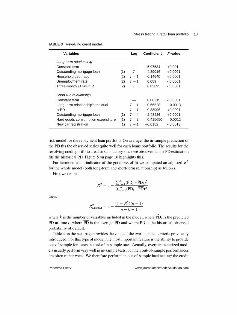
TABLE 3 Revolving credit model.

Variables Lag Coefficient P-value

Long-term relationshipConstant term — �5.97534 <0.001Outstanding mortgage loan (1) T �4.39016 <0.0001Household debt ratio (2) T � 1 0.14640 <0.0001Unemployment rate (2) T � 1 0.089 <0.0001Three-month EURIBOR (2) T 0.03895 <0.0001

Short run relationshipConstant term — 0.00215 <0.0001Long-term relationship’s residual T � 1 �0.66528 0.0013�PD T � 1 0.38996 <0.0001Outstanding mortgage loan (3) T � 4 �2.48486 <0.0001Hard goods consumption expenditure (1) T � 2 �0.415650 0.0012New car registration (1) T � 1 �0.0152 <0.0013

risk model for the repayment loan portfolio. On average, the in-sample prediction ofthe PD fits the observed series quite well for each loans portfolio. The results for therevolving credit portfolio are also satisfactory since we observe that the PD estimationfits the historical PD. Figure 5 on page 16 highlights this.

Furthermore, as an indicator of the goodness of fit we computed an adjusted R2

for the whole model (both long-term and short-term relationship) as follows.First we define:

R2 D 1 �

PniD1.PDi �cPDi /2PniD1.PDi �PD/2

then:

R2adjusted D 1 �.1 �R2/.n � 1/

n � k � 1

where k is the number of variables included in the model, where cPDi is the predictedPD at time i , where PD is the average PD and where PD is the historical observedprobability of default.

Table 4 on the next page provides the value of the two statistical criteria previouslyintroduced. For this type of model, the most important feature is the ability to provideout-of-sample forecasts instead of in-sample ones. Actually, overparameterized mod-els usually perform very well in in-sample tests, but their out-of-sample performancesare often rather weak. We therefore perform an out-of-sample backtesting: the credit


14 S. Assouan

TABLE 4 Statistical criteria.

Root meansquared

R2adjusted error

Repayment loan 0.867 0.0226Revolving credit 0.957 0.018

FIGURE 2 Observed default rates versus prediction: repayment loan.

2001 Q1 2003 Q1 2005 Q1 2007 Q1 2009 Q15.0

5.5

6.0

6.5

7.0

7.5

%

Repayment loanPredicted value

risk model is estimated on a quarterly sample from 2001 Q1 to 2008 Q4. We thenperform an out-of-sample forecast from 2009 Q1 to 2010 Q2.4

Figure 4 on the facing page shows the observed and predicted values of PD whenthe model’s parameters are estimated from 2001 Q1 to 2008 Q4. The differencesbetween observed and predicted values are generally small. However, the repaymentloan’s model has much more difficulty predicting the PD than the revolving creditmodel. Indeed, the repayment loan model underestimates the PD over the backtestingperiod even if it fits the PD dynamic quite well.

4 PDs for 2010 Q1 and 2010 Q2 were not available when the model was built.



FIGURE 3 In-sample observed default rates versus prediction: revolving credit.

2001 Q1 2003 Q1 2005 Q1 2007 Q1 2009 Q11.2

1.4

1.6

1.8

2.0

2.2

%

Revolving creditPredicted value

FIGURE 4 Backtesting out of sample: repayment loan.

2001 Q1 2003 Q1 2005 Q1 2007 Q1 2009 Q15.0

5.5

6.0

6.5

7.0

7.5

%

Repayment loanPredicted value

2010 Q2

Estimation period Backtesting

5.3 Stress scenario

The stress scenarios (both baseline and adverse) used in this paper have been definedby the European Banking Authority for the 2011 stress-test exercise. The objective


16 S. Assouan

FIGURE 5 Backtesting out of sample: revolving credit.

2001 Q1 2003 Q1 2005 Q1 2007 Q1 2009 Q1

Estimation period Backtesting

1.2

1.4

1.6

1.8

2.0

2.2

%

Revolving creditPredicted value

2.4

was to assess the resilience of a large sample of banks in the EU5 against an adversebut plausible scenario. The scenario assesses banks against a deterioration from thebaseline forecast in the main macroeconomic variables such as GDP, unemploymentand house prices. For example, GDP would fall four percentage points from thebaseline. Moreover, changes in interest rates and sovereign spreads also affect thecost of funding for banks under the stress. Crédit Agricole economists, with respectto the European Banking Authority’s stress scenarios, designed these scenarios formore specific variables such as household investment, household real disposal income,outstanding mortgage credit, etc. Table 5 on the facing page presents both scenariosused for stress testing.

5.4 Application to the credit risk model

5.4.1 Repayment loan

Let us recall the general framework of our macroeconomic credit risk model built forboth portfolios:

Yt D ˛Xt C "t

�Yt D � O"t�1 C ��Xt C �Zt C �t

)(5.1)

where Yt is the historical PD, where Xt is a vector of I.1/ variables, where Zt is avector of stationary variables and where "t and �t are two random terms assumed to

5 This includes non-EU European Economic Area banks where appropriate.



TABLE 5 Stress scenario.

Baseline Adverse‚ …„ ƒ ‚ …„ ƒ2010 Q4 2011 2012 2011 2012

Variables (%) (%) (%) (%) (%)

(1) LevelUnemployment rate 9.3 9.5 9.2 9.6 9.8Inflation rate C1.5 C1.6 C1.6 1.3 0.9Three-month EURIBOR 1 1.5 1.8 2.75 2.75Household debt ratio 79.3 82.1 85.2 78.9 76.9

(2) Growth rateOutstanding mortgage loan C8.2 C8.4 C7.9 C2.0 �2.0Household investment �2.2 C2.3 C2.6 �2.0 �5.5Real disposable income C2.6 C3.0 C2.8 C1.5 C0.5New cars registration �3.0 �2.0 �3.0 �6.0 �3.0

FIGURE 6 Stress testing for the repayment loan portfolio.

2001 Q1 2003 Q1 2005 Q1 2007 Q1 2009 Q1 2011 Q15.0

5.5

6.0

6.5

7.0

7.5

%

8.0Repayment loanBaselineAdverse

be independent, identically and normally distributed. By iterating the model forwardover the two-year horizon we obtain Figure 6.

Figure 6 presents the evolution of the default rates of the repayment loan portfoliounder the baseline and the adverse scenarios. Figure 7 on the next page presents theevolution of the default rates of the revolving credit portfolio under the baseline and the


18 S. Assouan

FIGURE 7 Stress testing for the revolving credit portfolio.

2001 Q1 2003 Q1 2005 Q1 2007 Q1 2009 Q1 2011 Q1

Revolving creditBaselineAdverse

1.2

1.4

1.6

1.8

2.0

2.2

%

2.4

adverse scenarios. For the repayment loan portfolio under the baseline scenario, thedefault rate has decreased from 7.28% in 2010 Q4 to 6.65% in 2012 Q4; by contrast,the PD reaches 7.69% under the adverse scenario. Finally, the model provides a�8.68% impact on the baseline scenario and a 5.54% increase on the adverse one.For the revolving credit portfolio, as presented in Figure 3 on page 15, the default ratehas decreased under the baseline scenario from 1.91% to 1.88% between 2010 Q4 and2012 Q4, which means an impact on the PD of�1.61%. In contrast, under the adversescenario, the default rate rises to 2.15%. These results (for both portfolios) show thesensitivity of the PD to the macroeconomic variables in the scenario, defending ourstress-test approach. Indeed, experts expected a slight decrease in the default ratesunder the baseline scenario and a sharp rise under the adverse scenario. Table 6 onthe facing page gives more details.

6 CONCLUSION

In this paper we have investigated a time series model, specifically an ECM, for stresstesting a retail loan portfolio. A distinguishing feature of the study is the applicationof this approach for stress testing to a retail loan portfolio. Indeed, this time seriesapproach is normally developed for corporate or sovereign loans portfolios. Withinthe time series framework, we choose an ECM since we consider key macroeconomicvariables to be exogenous to the model. Moreover, this macroeconomic credit riskmodel is based on the assumption that the PD of a retail loan portfolio is influenced by



TABLE 6 PD impact.

Impact: Impact:2010 2010

2010 2011 versus 2012 versusQ4 Q4 2011 Q4 2012

Scenario (%) (%) (%) (%) (%)

Repayment loanBaseline 7.28 6.54 �10.18 6.65 �8.68

Adverse 7.28 6.77 �7.07 7.69 C5.54

Revolving creditBaseline 1.91 1.91 �0.19 1.88 �1.61

Adverse 1.91 2.03 C5.98 2.15 C12.19

key macroeconomic variables through a cointegration relationship. This assumptionhas been validated by several stationarity and cointegration tests.

The empirical results show a significant and robust relationship between theportfolio’s PD and several macroeconomic variables, including some consumption-loan-specific variables. In addition, the macroeconomic credit risk models obtainedare economically consistent with respect to the out-of-sample backtesting results.The repayment loan model suggests a decrease of PD under the baseline scenarioand a sharp increase under the adverse scenario. On the other hand, the revolv-ing credit portfolio model suggests a steady evolution of the PD with some fluc-tuations under the baseline scenario, whereas the results under the adverse sce-nario show a sharp rise in PD. These results are close to what stress-test man-agers expected. Finally, the impacts in terms of PD under the adverse scenario arealways greater than the baseline ones. We believe that these very simple modelsare well-suited to retail portfolios. Indeed, the outstanding loan balance of a retailloan portfolio being less than the corporate portfolio, assuming the endogeneity ofall the variables (PD and macroeconomic factors) as in a VAR model, is an unre-alistic assumption. In other words, it is unrealistic to consider that a change in PDof a Crédit Agricole repayment loan or revolving credit portfolio affects France’sGDP.

An interesting direction for future research would be the integration of the otherrisk parameters, especially LGD, to this type of model. We would then be able tocompute a loss distribution without considering LGD parameters as a constant term.Another idea would be to use more robust stationarity and cointegration tests due tothe weakness of the number of observations. The improvement of historical data isobviously a way to improve the robustness of the models.


20 S. Assouan

APPENDIX A: ERROR CORRECTION MODEL

A.1 Principles

An ECM assumes the following specification:

Yt D ˛Xt C "t

�Yt D � O"t�1 C ��Xt C �Zt C �t

)(A.1)

where �yt is the first difference of yt , ie, �yt D yt � yt�1, and where ˛, � and �are a set of coefficients to be estimated. "t and �t are random terms assumed to beindependent, identically and normally distributed. The first equation of (A.1), whichis called a long-term relationship, considers a long-term equilibrium between X andY . ThenX and Y are supposed to have a joint evolution and not to differ significantlyover time. When they differ, " is meant to correct the temporary imbalance in the short-term relationship (second equation of (A.1)). Therefore, at each step t , "t�1 allowsthe correction of the previous estimation of Y . This is the error correction mechanism.

Note that lagged values of the first difference of Y could be included in (A.1).Equation (A.1) is valid if and only if

� Y and X are integrated (see (A.3) for details) of the same order,

� " is stationary (see (A.2) for details), which implies that X and Y are cointe-grated,

� Z is stationary,

� � is both negative and statistically significant.

The following section introduces two concepts that are fundamental to the under-standing of an ECM.

A.2 Stationarity and unit root tests

A stationary process has the property that the mean, variance and autocorrelationstructure do not change over time. Consider the following processes:

xt D �xt�1 C ut ; j�j < 1 (A.2)

yt D yt�1 C vt (A.3)

The error terms ut and vt are assumed to be normally independently identicallydistributed with zero mean and unit variance, ut , vt � iin.0; 1/, ie, a purely randomprocess. Both xt and yt are AR(1) models. By calculating the mean, variance andautocovariance xt and yt , we can show that the means of the two series are:

E.xt / D 0 and E.yt / D 0 (A.4)



and the variances are:

V.xt / D

t�1XiD0

�2i var.ut�i /! Œt !1�1

1 � �2

V.yt / D

t�1XiD0

var.vt�i / D t

The autocovariances of the two series are:

�x.h/ D E.xt ; xtCh/ D

tCh�1XiD0

�i�hCi

�y.h/ D E.yt ; ytCh/ D t � h

If the means of xt and yt are equals, they differ by their variances and their autoco-variances. But the most important result is that the variance and autocovariance ofyt are functions of t , contrary to xt . Then, as t increases, the variance and autoco-variance of yt increase while those of xt converge to a constant. By considering thedefinition of a stationary process, we conclude that xt is stationary, whereas yt is anonstationary process. yt is a nonstationary process because of the unit root.6 As aconsequence, the presence of a unit root indicates that a time series is not stationary.xt is said to be difference-stationary.

There exists another type of nonstationary process. Thus, if we considered a con-stant (drift) term with or without a deterministic trend in (A.2) and (A.3), we wouldhave the same type of results about the mean,7 the variance and the autocovarianceof xt and yt . Within a deterministic trend, yt is said to be trend-stationary.

With respect to the presence of a constant term and/or a deterministic trend, ytcould be transformed to a stationary process using one of the following methods.

� Differencing once, ie, �yt D .1 � L/yt D yt � yt�1 D vt , where L is a lagoperator.

� Detrending (the trend ˇt is subtracted), ie:

yt D ˛ C ˇt C "t ) yt � ˇt D ˛ C "t

� Detrending, then differencing the detrended process.

6 yt is a special case of an xt process when � D 1.7 With a constant term, E.xt / D ˛=.1 � �/ and E.yt / D ˛t .


22 S. Assouan

Since Dickey and Fuller (1979), an enormous number of studies of stationarity testshave appeared, and several statistical tests have been implemented. In this paper weperform the Dickey–Fuller (DF) test (and its augmented version when necessary), theERS test, the Phillips–Perron (PP) test and the SP test. Maddala and Kim (1998) givemore details on these stationarity tests.

Since the decision regarding the integration order (see Section A.3 for details) is adetermining step of the modeling process, we chose to use several stationarity tests.Thus, the integration order is chosen by considering the power and the robustnessof each test. Salanié (1999) shows that the SP test for stationarity is the most robustand that the ERS stationarity test is the most powerful among the stationarity tests.As a result, priority is given to the results of these two stationary tests because thereduced size of the data (thirty-six observations) could lead a time series to be wronglyconsidered as stationary.

A.3 Integration order and cointegration

If a nonstationary time series can be transformed into a stationary one by differencingonce, then this series is said to be integrated of order one or I.1/. Some time seriescould require k repeated differences to obtain a stationary process, they are said tobe integrated of order k. In addition, stationary variables are said to be I.0/.

In general, regression models for nonstationary variables give spurious results.For example, Granger and Newbold (1974) present some examples with artificiallyand independently generated data so that there is no relationship between two timeseries z1;t and z2;t . However, the correlations between z1;t and z1;t�1 and betweenz2;t and z2;t�1 were high. The regression of z1;t on z2;t gave a high coefficient ofdetermination (R2) but a low Durbin–Watson statistic. They also run the regressionin first difference, for which theR2 is close to zero and the Durbin–Watson statistic isclose to two. This demonstrates that there is no relationship between z1;t�1 and z2;tand that the R2 obtained was spurious.

Regression models for nonstationary time series only make sense if they are saidto be cointegrated. The concept of cointegration was first introduced by Engle andGranger (1987) so that two I.1/ variables yt and xt are said to be cointegrated ifthere exists ˇ such that yt � ˇxt is I.0/. The concept could be generalized for twoor more I.d/ variables: two I.d/ variables yt and xt are said to be cointegrated ifthere exists ˇ such that yt � ˇxt is I.d � b/ with b > 0.

Several cointegration tests have been introduced in the literature and used in prac-tice. The principle of these tests is to test whether two or more integrated variablesdeviate significantly from a certain relationship. While cointegration tests can be per-formed in a single equation framework or in systems of multiple equations, this paperwill only discuss cointegration tests in a single equation framework.



TABLE A.1 Integration order of macroeconomic variables.

Integration order Final‚ …„ ƒ integrationVariable DF PP SP ERS order

Inflation (twelve months) I.1/ I.1/ I.0/ I.1/ I.1/

Household debt ratio (consumer credit) I.1/ I.1/ I.0/ I.0/ I.0/

Household investment I.1/ I.1/ I.1/ I.1/ I.1/

Ten-year interest rate I.1/ I.1/ I.1/ I.1/ I.1/

Outstanding mortgage credit I.0/ I.1/ I.1/ I.1/ I.1/

CAC 40 index I.0/ I.0/ I.0/ I.0/ I.0/

Corporate debt ratio I.1/ I.1/ I.1/ I.1/ I.1/

Consumption loan interest rate I.1/ I.1/ I.1/ I.1/ I.1/

Household debt ratio I.1/ I.1/ I.1/ I.1/ I.1/

Outstanding consumer credit I.0/ I.1/ I.0/ I.0/ I.0/

Corporate investment I.0/ I.0/ I.0/ I.0/ I.0/

Mortgage’s interest rate I.1/ I.1/ I.0/ I.1/ I.1/

New car registration I.0/ I.0/ I.0/ I.0/ I.0/

Quarterly inflation I.1/ I.1/ I.0/ I.1/ I.1/

Industrial output I.0/ I.0/ I.1/ I.0/ I.0/

Hard goods consumption expenditure I.0/ I.0/ I.1/ I.0/ I.0/

The most commonly used cointegration test is the Engle and Granger (1987) two-step approach, which is known as a residual-based test (the first test of its kind forcointegration). Consider a set of .k C 1/ I.1/ variables: a vector of k explanatoryvariables Xt and a variable of interest yt . If there exists a vector ˇ such that yt �ˇ0Xt is I.0/, then ˇ is the cointegrating vector. The residual-based tests consider theequation:

yt D ˇ0Xt C "t (A.5)

If "t has a unit root, ie, it is not stationary, then yt � ˇ0Xt is not a cointegratingrelationship. Thus, a test for a unit root in "t is meant to test that the variables ytand Xt are not cointegrated. In practice, ˇ and " are not observed; they are estimatedby OLS or GLS regressions and a unit root test is performed on O"t . Yet because "tis not observed, different critical values have been tabulated to test the presence ofa unit root in the Engle and Granger approach. The stationarity of " implies thaty and X are cointegrated, so the cointegration’s hypothesis will be rejected in thecase of nonstationarity of "t . In this paper the PP test is used to test the stationarityof O"t .


24 S. Assouan

REFERENCES

Åsberg, P., and Shahnazarian, H. (2008). Macroeconomic impact on expected default fre-quency. Working Paper 220, Sveriges Riksbank.

Avouyi-Dovi, S., Bardos, M., Jardet, C., Kendaoui, L., and Moquet, J. (2009). Macro stresstesting with a macroeconomic credit risk model: application to the French manufacturingsector. Working Paper 238, Banque de France.

Basel Committee on Banking Supervision (2009). Principles for sound stress testing prac-tices and supervision. Consultative Document, BIS (May).

Basurto, M., and Padilla, P. (2006). Portfolio credit risk and macroeconomic shocks: appli-cations to stress testing under data-restricted environments. Working Paper 06/283,International Monetary Fund.

Bucay, N., and Rosen, D. (2001). Applying portfolio credit risk models to retail porfolios.Journal of Risk Finance 2(3), 35–61.

Davidson, J. E. H., Hendry, D. F., Srba, F., and Yeo, S. (1978). Econometric modelling ofthe aggregate time series relationships between consumer’s expenditure and income inthe United Kingdom. Economic Journal 88, 661–692.

Dickey, D. A., and Fuller, W. A. (1979). Distribution of the estimators for autoregressive timeseries with a unit root. Journal of the American Statistical Association 74, 427–431.

Engle, R., and Granger, J. (1987). Co-integration and error correction: representation, esti-mation and testing. Econometrica 55(2), 251–276.

Foglia, A. (2008). Stress testing credit risk: a survey of authorities’ approaches. OccasionalPaper 37, Economic Research Department, Bank of Italy.

Granger, C. W. J., and Newbold, P. (1974). Spurious regression in econometrics. Journalof Econometrics 2, 111–120.

Hoggarth, G., Sorensen, S., and Zicchino, L. (2005). Stress tests of UK banks using a VARapproach. Working Paper 282, Bank of England.

MacKinnon, J. G. (2010). Critical values for cointegration tests. Working Paper 1227, Eco-nomics Department, Queen’s University.

Maddala, G. S., and Kim, I.-M. (1998). Unit Roots, Cointegration, and Structural Change.Cambridge University Press.

Merton, R. C. (1974). On the pricing of corporate debt: the risk structure of interest rates.Journal of Finance 29, 449–470.

Misina, M., and Tessier, D. (2008). Non-linearities, model uncertainty, and macro stresstesting. Working Paper 2008-30, Bank of Canada.

Misina, M., Tessier, D., and Shubhasis, D. (2006). Stress testing the corporate loans port-folio of the Canadian banking sector. Working Paper 2006-47, Bank of Canada.

Ouliaris, S., and Phillips, P. C. B. (1990). Asymptotic properties of residual based tests forcointegration. Econometrica 58(1), 165–193.

Rösch, D., and Scheule, H. (2007). Stress-testing credit risk parameters: an application toretail loan portfolios. The Journal of Risk Model Validation 1(1), 55–75.

Salanié, B. (1999). Guide pratique des séries non stationnaires. Economie et Prévision137, 119–141.

Sorge, M. (2004). Stress-testing financial systems: an overview of current methodologies.Working Paper 165, Bank for International Settlements (December).



Virolainen, K. (2004). Macro stress testing with a macroeconomic credit risk model forFinland. Discussion Paper 18/2004, Bank of Finland.

Wilson, T. C. (1997a). Portfolio credit risk. I. Risk 10(9), 111–117.Wilson, T. C. (1997b). Portfolio credit risk. II. Risk 10(10), 56–57.


Date post:	07-May-2018
Category:	Documents
Upload:	vuhanh
View:	214 times
Download:	0 times

Stress testing a retail loan portfolio: an error ... · The Journal of Risk Model Validation...

Documents