arXiv:1709.03506v4 [hep-th] 25 Oct 2018 String Geometry and Non-perturbative Formulation of String Theory Matsuo Sato 1 Department of Natural Science, Faculty of Education, Hirosaki University Bunkyo-cho 1, Hirosaki, Aomori 036-8560, Japan Abstract We define string geometry: spaces of superstrings including the interactions, their topologies, charts, and metrics. Trajectories in asymptotic processes on a space of strings reproduce the right moduli space of the super Riemann surfaces in a target manifold. Based on the string geometry, we define Einstein-Hilbert action coupled with gauge fields, and formulate superstring theory non-perturbatively by summing over metrics and the gauge fields on the spaces of strings. This theory does not depend on backgrounds. The theory has a supersymmetry as a part of the diffeomorphisms symmetry on the superstring manifolds. We derive the all-order perturbative scattering amplitudes that possess the super moduli in type IIA, type IIB and SO(32) type I superstring theories from the single theory, by considering fluctuations around fixed backgrounds representing type IIA, type IIB and SO(32) type I perturbative vacua, respectively. The theory predicts that we can see a string if we microscopically observe not only a particle but also a point in the space-time. That is, this theory unifies particles and the space-time. 1 e-mail address : [email protected]
Transcript
arX
iv:1
709.
0350
6v4
[he
p-th
] 2
5 O
ct 2
018
String Geometry and Non-perturbative Formulation of String Theory
Matsuo Sato1
Department of Natural Science, Faculty of Education, Hirosaki University
Bunkyo-cho 1, Hirosaki, Aomori 036-8560, Japan
Abstract
We define string geometry: spaces of superstrings including the interactions, theirtopologies, charts, and metrics. Trajectories in asymptotic processes on a space ofstrings reproduce the right moduli space of the super Riemann surfaces in a targetmanifold. Based on the string geometry, we define Einstein-Hilbert action coupledwith gauge fields, and formulate superstring theory non-perturbatively by summingover metrics and the gauge fields on the spaces of strings. This theory does not dependon backgrounds. The theory has a supersymmetry as a part of the diffeomorphismssymmetry on the superstring manifolds. We derive the all-order perturbative scatteringamplitudes that possess the super moduli in type IIA, type IIB and SO(32) type Isuperstring theories from the single theory, by considering fluctuations around fixedbackgrounds representing type IIA, type IIB and SO(32) type I perturbative vacua,respectively. The theory predicts that we can see a string if we microscopically observenot only a particle but also a point in the space-time. That is, this theory unifiesparticles and the space-time.
3 Perturbative string amplitudes from string geometry 10
4 Superstring geometry 24
5 Including open strings 41
6 Non-perturbative formulation of superstring theory 49
7 Matrix models for superstring geometry 59
8 Heterotic construction 60
9 Conclusion 80
10 Discussion 81
1 Introduction
In the T-duality and its generalization, the mirror symmetry, there is a coincidence between
geometric invariants of two different manifolds. It is thought that the reason for this is
that the spaces observed by the strings are the same although they are in the different
target manifolds. Therefore, the space observed by the strings, which is invariant under
the T-duality and mirror transformations, will be a geometric principle of string theory. A
moduli space in a target manifold, which is a collection of on-shell embedding functions of
the Riemann surfaces Xµ(σ, τ), is invariant under the T-duality transformations. Actually,
the T-duality rule ∂aXµ(σ, τ) = iǫab∂
bX′µ(σ, τ) gives an one-to-one correspondence between
the on-shell embedding functions of the Riemann surfaces Xµ(σ, τ) and X′µ(σ, τ). Moreover,
the Riemann surfaces in the target manifold can be generated by trajectories in a space of
1
strings. Therefore, a space of strings will be the geometric principle1.
Furthermore, string theory as a quantum gravity also suggests that a space of strings
will be a geometric principle of string theory as follows. It has not succeeded to obtain
ordinary relativistic quantum gravity that is defined by a path integral over metrics on a
space representing the spacetime itself because of ultraviolet divergences. The reason would
be impossibility to regard points as fundamental constituents of the spacetime because the
spacetime itself fluctuates at the Plank scale. Thus, it is reasonable to define quantum
gravity by a path integral over metrics on a space that consists of strings, by making a point
have a structure of strings. In fact, perturbative strings are shown to suppress the ultraviolet
divergences in quantum gravity.
In this paper, we geometrically define a space of superstrings including the effect of
interactions. For this purpose, here we first review how such spaces of strings are defined
in string field theories. In these theories, after a free loop space of strings are prepared,
interaction terms of strings in actions are defined. In other words, the spaces of strings are
defined by deforming the ring on the free loop space. Geometrically, the space of strings is
defined by deformation quantization of the free loop space as a noncommutative geometry.
Actually, in Witten’s cubic open string field theory [5], the interaction term is defined by
using the ∗-product of noncommutative geometry. On the other hand, we adopt different
approach, namely (infinite-dimensional) manifold theory2. We do not start with a free
loop space, but we define a space of strings including the effect of interactions from the
beginning. The criterion to define a topology, which represents how near the strings are, is
that trajectories in asymptotic processes on the space of strings reproduce the right moduli
space of the super Riemann surfaces in a target manifold. We need Riemannian geometry
1Recently, in the homological mirror symmetry [1], it is shown in [2] that the moduli space of the pseudoholomorphic curves in the A-model on a symplectic torus is homeomorphic to a moduli space of Feynmandiagrams in the configuration space of the morphisms in the B-model on the corresponding elliptic curve.Therefore, a dynamical and non-perturbative generalization of the moduli space of the pseudo holomorphiccurves will be the geometric principle of string theory. Here we discuss this generalization. First, a modulispace of pseudo holomorphic curves is defined even in closed string theory in [3]. Moreover, the modulispace can be defined by restricting a moduli space of curves, which is not necessarily holomorphic, to theholomorphic sector [4]. Because this is a restriction to the topological string theory, the moduli space ofcurves is the dynamical generalization. Furthermore, the curves can be generated by trajectories in a spaceof strings. Therefore, a space of strings will be the dynamical and non-perturbative generalization, that isthe geometric principle.
2See [6] as an example of text books for infinite-dimensional manifolds
2
naturally for fields on the space of strings because it is not flat3.
By adopting the space of superstrings as geometric principle, we formulate superstring
theory non-perturbatively. That is, we formulate the theory by summing over metrics on
the space of strings. As a result, the theory is independent of backgrounds.
The organization of the paper is as follows. In section 2, we define string geometry and
its Einstein-Hilbert action coupled with gauge fields. In section 3, we solve the equations of
motion and obtain a string geometry solution that represents perturbative string vacuum.
We derive the propagator of the fluctuations around the solution. Then, we move to the first
quantization formalism, and we derive the all-order perturbative scattering amplitudes that
possess its moduli in string theory. We extend these results to a supersymmetric theory in
section 4, to a theory including open strings in section 5, and to a supersymmetric theory
including open superstrings in section 6. The theory in section 6 is a non-perturbatively
formulated superstring theory. We derive the all-order perturbative scattering amplitudes
that possess the super moduli in type IIA, type IIB and SO(32) type I superstring theories
from the single theory, by considering fluctuations around fixed backgrounds representing
type IIA, type IIB and SO(32) type I perturbative vacua, respectively. In section 7, we
discuss a relation between the superstring geometry and supersymmetric matrix models of
a new type. In section 8, based on superstring geometry, we formulate and study a theory
that manifestly possesses the SO(32) and E8 ×E8 heterotic perturbative vacua. We expect
that this theory is equivalent to the theory in section 6, which manifestly possesses the type
IIA, type IIB and SO(32) type I perturbative vacua. We conclude in section 9 and discuss
in section 10.
2 String geometry
Let us define unique global time on a Riemann surface Σ with punctures P i (i = 1, · · · , N)
in order to define string states by world-time constant lines. On Σ, there exists an unique
Abelian differential dp that has simple poles with residues f i at P i where∑
i fi = 0, if it is
normalized to have purely imaginary periods with respect to all contours to fix ambiguity
3The spaces of strings in string field theories are different with those in string geometry because non-commutative geometry and Riemannian geometry describe different spaces.
3
of adding holomorphic differentials. A global time is defined by w = τ + iσ :=∫ P
dp at
any point P on Σ [7, 8]. τ takes the same value at the same point even if different contours
are chosen in∫ P
dp, because the real parts of the periods are zero by definition of the
normalization. In particular, τ = −∞ at P i with negative f i and τ = ∞ at P i with positive
f i. A contour integral on τ constant line around P i: i∆σ =∮
dp = 2πif i indicates that the
σ region around P i is 2πf i. This means that Σ around P i represents a semi-infinite cylinder
with radius f i. The condition∑
i fi = 0 means that the total σ region of incoming cylinders
equals to that of outgoing ones if we choose the outgoing direction as positive. That is, the
total σ region is conserved. In order to define the above global time uniquely, we fix the σ
regions 2πf i around P i. We divide N P is to arbitrary two sets consist of N− and N+ P is,
respectively (N−+N+ = N), then we divide -1 to N− f i ≡ −1N−
and 1 to N+ f i ≡ 1N+
equally
for all i.
Thus, under a conformal transformation, one obtains a Riemann surface Σ that has
coordinates composed of the global time τ and the position σ. Because Σ can be a moduli
of Riemann surfaces, any two-dimensional Riemannian manifold Σ can be obtained by Σ =
ψ(Σ) where ψ is a diffeomorphism times Weyl transformation.
Next, we will define the model space E. We consider a state (Σ, X(τs), τs) determined
by Σ, a τ = τs constant line and an arbitrary map X(τs) from Σ|τs to the Euclidean space
Rd. Σ is a union of N± cylinders with radii fi at τ ≃ ±∞. Thus, we define a string state as
an equivalence class [Σ, X(τs ≃ ±∞), τs ≃ ±∞] by a relation (Σ, X(τs ≃ ±∞), τs ≃ ±∞) ∼(Σ′, X ′(τs ≃ ±∞), τs ≃ ±∞) if N± = N ′
±, fi = f ′i , and X(τs ≃ ±∞) = X ′(τs ≃ ±∞) as in
Fig. 1. Because Σ|τs ≃ S1 ∪ S1 ∪ · · · ∪ S1 and X(τs) : Σ|τs → M , [Σ, X(τs), τs] represent
many-body states of strings in Rd as in Fig. 2. The model space E is defined by a collection
of all the string states [Σ, X(τs), τs].Here, we will define topologies of E. We define an ǫ-open neighbourhood of [Σ, Xs(τs), τs]
Figure 1: An equivalence class of a string state [Σ, X(τs ≃ −∞), τs ≃ −∞]. If the cylindersand the embedding functions are the same at τ ≃ −∞, the states of strings at τ ≃ −∞specified by the red lines (Σ, X(τs ≃ −∞), τs ≃ −∞), (Σ′, X ′(τs ≃ −∞), τs ≃ −∞), and(Σ′′, X ′′(τs ≃ −∞), τs ≃ −∞) should be identified.
PSfrag replacements
τ1
τ2
τ3
Rd
Figure 2: Various string states. The red and blue lines represent one-string and two-stringstates, respectively.
5
τs ≃ ±∞ constant line traverses only cylinders overlapped by Σ and Σ′. U is defined to be
an open set of E if there exists ǫ such that U([Σ, X(τs), τs], ǫ) ⊂ U for an arbitrary point
[Σ, X(τs), τs] ∈ U .
Let U be a collection of all the open sets U . The topology of E satisfies the axiom of
topology (i), (ii), and (iii).
(i) ∅, E ∈ U(ii) U1, U2 ∈ U ⇒ U1 ∩ U2 ∈ U(iii) Uλ ∈ U ⇒ ∪λ∈ΛUλ ∈ U .
Proof. (i) Clear.
(ii) If U1 ∩ U2 = ∅, it is clear. Let us consider the case U1 ∩ U2 6= ∅. Because U1, U2 ⊂U , there exist ǫ and ǫ′ such that U([Σ, X(τs), τs], ǫ) ⊂ U1 and U([Σ, X(τs), τs], ǫ
′) ⊂ U2
for all [Σ, X(τs), τs] ∈ U1 ∩ U2. Let ǫ′′ := min(ǫ, ǫ′). Because U([Σ, X(τs), τs], ǫ′′) ⊂
ǫ′′ such that U([Σ, X(τs), τs], ǫ′′) ⊂ U1 ∩ U2 for all [Σ, X(τs), τs] ∈ U1 ∩ U2.
(iii) If ∪λ∈ΛUλ = ∅, it is clear. Let us consider the case ∪λ∈ΛUλ 6= ∅. For all [Σ, X(τs), τs] ∈∪λ∈ΛUλ, there exists λ0 such that [Σ, X(τs), τs] ∈ Uλ0 . Because Uλ0 ∈ U , there is ǫ such
that U([Σ, X(τs), τs], ǫ) ⊂ Uλ0 . Then, U([Σ, X(τs), τs], ǫ) ⊂ ∪λ∈ΛUλ for all [Σ, X(τs), τs] ∈∪λ∈ΛUλ.
Although the model space is defined by using the coordinates [Σ, X(τs), τs], the model
space does not depend on the coordinates, because the model space is a topological space.
In the following, we denote [hmn, X(τ), τ ], where hmn(σ, τ ) (m,n = 0, 1) is the worldsheet
metric of Σ, instead of [Σ, X(τ), τ ], because giving a Riemann surface is equivalent to giving
a metric up to diffeomorphism and Weyl transformations.
Next, in order to define structures of string manifold, we consider how generally we can
define general coordinate transformations between [hmn, X(τ), τ ] and [h′mn, X′(τ ′), τ ′] where
[hmn, X(τ), τ ] ∈ U ⊂ E and [h′mn, X′(τ ′), τ ′] ∈ U ′ ⊂ E. hmn does not transform to τ and
X(τ) and vice versa, because τ and X(τ) are continuous variables, whereas hmn is a discrete
variable: τ and X(τ) vary continuously, whereas hmn varies discretely in a trajectory on
E by definition of the neighbourhoods. τ and σ do not transform to each other because
the string states are defined by τ constant lines. Under these restrictions, the most general
6
PSfrag replacements
MM
t
τ
Σ Σ′t1 t2 t3
τ1
τ2
[Σ, x(τ (t1)), τ(t1)]
[Σ, x(τ(t2)), τ(t2)] = [Σ′, x′(τ (t2)), τ(t2)]
[Σ′, x′(τ (t3)), τ(t3)]
Figure 3: A continuous trajectory. In case of general τ(t) as in the left graph, string stateson different Riemann surfaces can be connected continuously in MD as [Σ, x(τ(t1)), τ(t1)]and [Σ′, x′(τ(t3)), τ(t3)] on the pictures.
We will show that MD has a structure of manifold, that is there exists a general coordi-
nate transformation between the sufficiently small neighbourhood around an arbitrary point
[Σ, xs(τs), τs] ∈ MD and an open set of E. There exists a general coordinate transformation
X(x) that satisfies ds2 = dxµdxνGµν(x) = dXµdXνηµν on an arbitrary point x in the ǫσ
open neighbourhood around xs(τs, σ) ∈ M , if ǫσ is sufficiently small. An arbitrary point
4 We extend the model space from E = [hmn(σ, τ ), Xµ(σ, τ ), τ ] to E = [h′
mn(σ′, τ ′), X ′µ(σ′, τ ′), τ ′]
by including the points generated by the diffeomorphisms σ 7→ σ′(σ) and τ 7→ τ ′(τ ).5These coordinate transformations are diffeomorphisms, and functions over the string manifolds, for
example metrics, are differentiable functions. These statements are justified mathematically by formulatingthe string manifolds as polyfolds. The reference volume of polyfolds is given in [9]. For example, see Example1.8. in [10]. Indeed, for example, at the interaction point where two strings becomes one string, a cusp formedwhere the two strings touch, smoothly connects with the one string in the framework of polyfolds.
7
[Σ, x(τ), τ ] in the ǫ := inf0≦σ<2π ǫσ open neighbourhood around [Σ, xs(τs), τs] satisfies
Because the tangent vector X(τ , σ) exists for each x(τ , σ), there exists a vector bundle
for 0 ≦ σ < 2π and its section X(τ). x(τ ) and X(τ) satisfy (2.6) on each σ, that is
X(τ) : Σ|τ → Rd. Therefore, there exists a general coordinate transformation between the
sufficiently small neighbourhood around an arbitrary point [Σ, xs(τs), τs] ∈ MD and an open
set of E: [Σ, x(τ ), τ ] 7→ [Σ, X(τ), τ ].
By definition of the ǫ-open neighbourhood, arbitrary two string states on a connected
Riemann surface in MD are connected continuously. Thus, there is an one-to-one correspon-
dence between a Riemann surface with punctures in M and a curve parametrized by τ from
τ = −∞ to τ = ∞ on MD. That is, curves that represent asymptotic processes on MD
reproduce the right moduli space of the Riemann surfaces in the target manifold.
By a general curve parametrized by t on MD, string states on different Riemann sur-
faces that have even different genera, can be connected continuously, for example see Fig. 3,
whereas different Riemann surfaces that have different genera cannot be connected continu-
ously in the moduli space of the Riemann surfaces in the target space. Therefore, the string
geometry is expected to possess non-perturbative effects.
The tangent space is spanned by ∂∂τ
and ∂∂Xµ(σ,τ)
as one can see from the ǫ-open neigh-
bourhood (2.1). We should note that ∂∂hmn
cannot be a part of basis that span the tangent
space, because hmn is just a discrete variable in E. The index of ∂∂Xµ(σ,τ)
can be (µ σ). We
define a summation over σ by∫
dσe(σ, τ), where e :=√
hσσ. This summation is invariant
under σ 7→ σ′(σ) and transformed as a scalar under τ 7→ τ ′(τ , X(τ)).
Riemannian string manifold is obtained by defining a metric, which is a section of an
8
inner product on the tangent space. The general form of a metric is given by
ds2(h, X(τ), τ)
= G(h, X(τ), τ )dd(dτ)2 + 2dτ
∫
dσe(σ, τ)∑
µ
G(h, X(τ), τ)d (µσ)dXµ(σ, τ)
+
∫
dσe(σ, τ)
∫
dσ′e(σ′, τ )∑
µ,µ′
G(h, X(τ), τ) (µσ) (µ′σ′)dXµ(σ, τ)dXµ′(σ′, τ).
(2.7)
We summarize the vectors as dXI (I = d, (µσ)), where dXd := dτ and dX(µσ) := dXµ(σ, τ ).
Then, the components of the metric are summarized as GIJ(h, X(τ), τ). The inverse of the
metric GIJ(h, X(τ), τ) is defined by GIJGJK = GKJGJI = δKI , where δ
dd = 1 and δµ
′σ′
µσ =
1e(σ,τ)
δµ′
µ δ(σ− σ′). The components of the Riemannian curvature tensor are given by RIJKL in
the basis ∂∂XI . The components of the Ricci tensor are RIJ := RK
IKJ = RdIdJ +
∫
dσeR(µσ)I (µσ) J .
The scalar curvature is
R := GIJRIJ
= GddRdd + 2
∫
dσeGd (µσ)Rd (µσ) +
∫
dσe
∫
dσ′e′G(µσ) (µ′σ′)R(µσ) (µ′σ′).
The volume is√G, where G = det(GIJ).
By using these geometrical objects, we formulate string theory non-perturbatively as
Z =
∫
DGDAe−S, (2.8)
where
S =1
GN
∫
DhDX(τ)Dτ√G(−R +
1
4GNG
I1I2GJ1J2FI1J1FI2J2). (2.9)
As an example of sets of fields on the string manifolds, we consider the metric and an u(1)
gauge field AI whose field strength is given by FIJ . The path integral is canonically defined by
summing over the metrics and gauge fields on M. By definition, the theory is background
independent. Dh is the invariant measure67 of the metrics hmn on the two-dimensional
Riemannian manifolds Σ. hmn and hmn are related to each others by the diffeomorphism
and the Weyl transformations.
6The invariant measure is defined implicitly by the most general invariant norm without derivatives forelements δhmn of the tangent space of the metric, ||δh||2 =
∆t := 1√N. A trajectory of points [Σ, X(τ), τ ] is necessarily continuous in MD so that
the kernel < hm+1, Xm+1(τm+1), τm+1|e−1NTmH |hm, Xm(τm), τm > in the third line is non-zero
when N → ∞. If we integrate out pτ (t) and pX(τ , t) by using the relation of the ADM
9The correlation function is zero if hi and hf of the in state do not coincide with those of the out states,because of the delta functions in the fifth line.
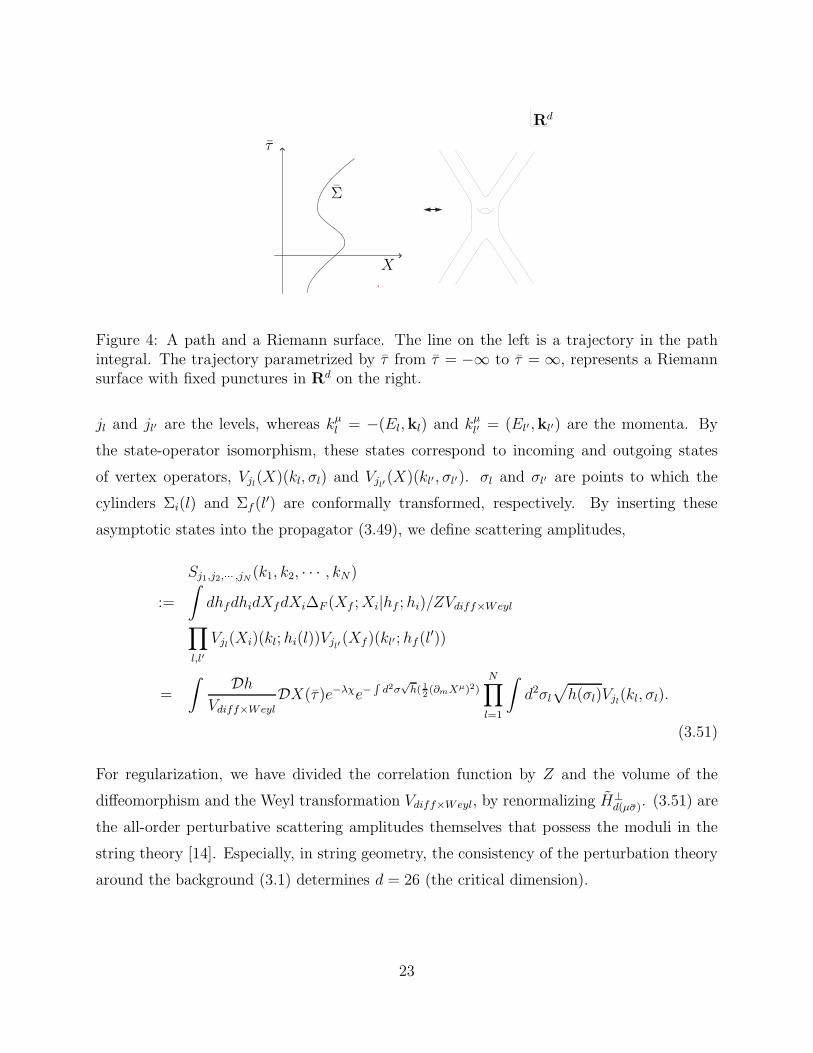
The path integral is defined over all possible two-dimensional Riemannian manifolds with
fixed punctures in Rd as in Fig. 4. The diffeomorphism times Weyl invariance of the action
in (3.48) implies that the correlation function in the string manifold MD is given by
∆F (Xf ;Xi|hf ; hi) = Z
∫ hf ,Xf
hi,Xi
DhDXe−λχe−Ss, (3.49)
where
Ss =
∫ ∞
−∞dτ
∫
dσ√
h(σ, τ)
(
1
2hmn(σ, τ)∂mX
µ(σ, τ)∂nXµ(σ, τ)
)
, (3.50)
and χ is the Euler number of the two-dimensional Riemannian manifold.
Here, we insert asymptotic states. Punctures exist only at τ = ±∞. We represent as
Vjl(Xi)(kl; hi(l)), an incoming asymptotic state on the incoming l-th cylinder Σi(l) in Σ at
τ ≃ −∞, where hi(l) denotes the metric on Σi(l) and l = 1, 2, · · · , m. Similarly, an outgoing
asymptotic state is denoted by Vjl′ (Xf )(kl′; hf(l′)) at τ ≃ ∞, where l′ = m+1, m+2, · · · , N .
22
PSfrag replacements
Rd
τ
X
Σ
Figure 4: A path and a Riemann surface. The line on the left is a trajectory in the pathintegral. The trajectory parametrized by τ from τ = −∞ to τ = ∞, represents a Riemannsurface with fixed punctures in Rd on the right.
jl and jl′ are the levels, whereas kµl = −(El,kl) and kµl′ = (El′ ,kl′) are the momenta. By
the state-operator isomorphism, these states correspond to incoming and outgoing states
of vertex operators, Vjl(X)(kl, σl) and Vjl′ (X)(kl′, σl′). σl and σl′ are points to which the
cylinders Σi(l) and Σf (l′) are conformally transformed, respectively. By inserting these
asymptotic states into the propagator (3.49), we define scattering amplitudes,
Sj1,j2,··· ,jN (k1, k2, · · · , kN):=
∫
dhfdhidXfdXi∆F (Xf ;Xi|hf ; hi)/ZVdiff×Weyl
∏
l,l′
Vjl(Xi)(kl; hi(l))Vjl′ (Xf)(kl′; hf (l′))
=
∫ DhVdiff×Weyl
DX(τ)e−λχe−∫d2σ
√h( 1
2(∂mXµ)2)
N∏
l=1
∫
d2σl√
h(σl)Vjl(kl, σl).
(3.51)
For regularization, we have divided the correlation function by Z and the volume of the
diffeomorphism and the Weyl transformation Vdiff×Weyl, by renormalizing H⊥d(µσ). (3.51) are
the all-order perturbative scattering amplitudes themselves that possess the moduli in the
string theory [14]. Especially, in string geometry, the consistency of the perturbation theory
around the background (3.1) determines d = 26 (the critical dimension).
23
4 Superstring geometry
In this section, we will define superstring geometry and derive perturbative superstring
amplitudes.
First, let us prepare a moduli space10 of type II superstring worldsheets Σ [15–17] with
punctures P i (i = 1, · · · , N)11. We consider two super Riemann surfaces ΣL and ΣR with
Neveu-Schwarz (NS) and Ramond (R) punctures whose reduced spaces ΣL,red and ΣR,red are
complex conjugates. A reduced space is defined by setting odd variables to zero in a super
Riemann surface. The complex conjugates means that they are complex conjugate spaces
with punctures at the same points. There are four types of punctures: NS-NS, NS-R, R-NS,
R-R because the punctures in ΣL and ΣR are not necessarily of the same type. A type
II superstring worldsheet Σ is defined by the subspace of ΣL × ΣR whose reduced space
ΣL,red × ΣR,red is restricted to its diagonal Σred.
Next, let us define global times uniquely on Σ in order to define string states by world-
time constant hypersurfaces. If there are R punctures on a super Riemann surface ΣR, the
superconformal structures have singularities on the R divisors [15–17]. On a R divisor, a
closed holomorphic 1-form takes the form, µ = w√2πidθ (mod z), which is uniquely determined
by an odd period w. On any other point, it takes the form, µ = b(z)dz + d(θα(z)). One
can define an even period∮
Sγ∗(µ) on a cycle S with dimension 1|0, where γ∗ is a pullback
by a map γ : S → ΣR. A- and B-periods on ΣR are defined by those on the reduced space
because∮
Sγ∗(µ) =
∮
Sredb(z)dz. The periods do not depend on a choice of reduced space
because they only depend on the homology class determined by the map γ if µ is closed.
Because the period of d(θα(z)) vanishes, we take the quotient of the space of 1-forms by
the subspace consisting of those whose periods vanish, and thus we have µ = b(z)dz. As a
result, on ΣR except for R-divisors, a closed holomorphic 1-form is uniquely determined by
even periods on the complete basis of A- and B-cycles.
Therefore, on ΣR, there exists an unique Abelian differential dp that has simple poles
with residues f i where∑
i fi = 0, at P i12, if it is normalized to have purely imaginary
10Strictly speaking, this should be called a parameter space of integration cycles [15,16] because superstringworldsheets are defined up to homology.
11P i not necessarily represents a point, whereas the corresponding P ired on a reduced space represents a
point. A Ramond puncture is located over a R divisor.12 The odd periods do not contribute to the residues because residues are defined around P i not on P i.
24
periods with respect to all contours to fix ambiguity of adding holomorphic differentials.
A global time is defined by w = τ + iσ :=∫ P
dp at any point P on ΣR13. By setting
the even coordinates to w under a superconformal transformation, a reduced space ΣR,red
is canonically defined. τ takes the same value at the same point even if different contours
are chosen in∫ P
dp, because the real parts of the periods are zero by definition of the
normalization. In particular, τ = −∞ at P i with negative f i and τ = ∞ at P i with positive
f i. A contour integral on τ constant line around P i: i∆σ =∮
dp = 2πif i indicates that
the σ region around P i is 2πf i. This means that ΣR around P i represents a semi-infinite
supercylinder with radius f i. The condition∑
i fi = 0 means that the total σ region of
incoming supercylinders equals to that of outgoing ones if we choose the outgoing direction
as positive. That is, the total σ region is conserved. In order to define the above global time
uniquely, we fix the σ regions 2πf i around P i. We divide N P is to arbitrary two sets consist
of N− and N+ P is, respectively (N− +N+ = N), then we divide -1 to N− f i ≡ −1N−
and 1 to
N+ f i ≡ 1N+
equally for all i.
If we give residues −f i and the same normalization on ΣL as on ΣR, we can set the
even coordinates on ΣL to the complex conjugate ¯w = τ − iσ :=∫ P
dp by a superconformal
transformation, because the Abelian differential is uniquely determined on ΣL and ΣL,red
is complex conjugate to ΣR,red. Therefore, we can define the global time τ uniquely and
reduced space canonically on the type II superstring worldsheet Σ.
Thus, under a superconformal transformation, one obtains a type II worldsheet Σ that
has even coordinates composed of the global time τ and the position σ and Σred is canoni-
cally defined. Because Σ can be a moduli of type II worldsheets with punctures, any two-
dimensional super Riemannian manifold with punctures Σ can be obtained by Σ = ψ(Σ)
where ψ is a superdiffeomorphism times super Weyl transformation [18, 19].
Next, we will define the model space E. We consider a state (Σ,X(τs), τs) determined by
Σ, a τ = τs constant hypersurface and an arbitrary map X(τs) from Σ|τs to the Euclidean
space Rd. Σ is a union of N± supercylinders with radii fi at τ ≃ ±∞. Thus, we define a
superstring state as an equivalence class [Σ,X(τs ≃ ±∞), τs ≃ ±∞] by a relation (Σ,X(τs ≃±∞), τs ≃ ±∞) ∼ (Σ′,X′(τs ≃ ±∞), τs ≃ ±∞) if N± = N ′
±, fi = f ′i , X(τs ≃ ±∞) =
X′(τs ≃ ±∞), and the corresponding supercylinders are the same type (NS-NS, NS-R, R-
13We define the integral by avoiding the R punctures and define the global time on P i by a limit to P i inorder that the odd periods do not contribute to the global time.
25
NS, or R-R) as in Fig. 1. Because the reduced space of Σ|τs is S1∪S1∪ · · · ∪S1 and X(τs) :
Σ|τs → Rd, [Σ,X(τs), τs] represent many-body states of superstrings in Rd as in Fig. 2. In
this supersymmetric case, we define the model space E such that E := ∪T [Σ,XT (τs), τs]where T runs IIA and IIB. IIA and IIB GSO projections are attached for T = IIA and IIB,
respectively. We can define the worldsheet fermion numbers of states in a Hilbert space
because the states consist of the fields over the local coordinates XµT = Xµ+ θαψµα+
12θ2F µ,
where ψµα is a Majorana fermion and F µ is an auxiliary field. We abbreviate T and (τs) of
Xµ, ψµα and F µ. We define the Hilbert space in these coordinates by the states only with
eπiF = 1 and eπiF = (−1)α for T = IIA, and eπiF = eπiF = 1 for T = IIB, where F and F are
left- and right-handed fermion numbers respectively, and α is 1 or 0 when the right-handed
fermion is periodic (R sector) or anti-periodic (NS sector), respectively.
Here, we will define topologies of E. An ǫ-open neighbourhood of [Σ,XTs(τs), τs] is
i , XT (τs ≃ ±∞) = X′T (τs ≃ ±∞), the corresponding supercylinders are
the same type (NS-NS, NS-R, R-NS, or R-R), and ǫ is small enough, because the τs ≃ ±∞constant hypersurfaces traverses only supercylinders overlapped by Σ and Σ
′. U is defined
to be an open set of E if there exists ǫ such that U([Σ,XT (τs), τs], ǫ) ⊂ U for an arbitrary
point [Σ,XT (τs), τs] ∈ U . In exactly the same way as in section 2, one can show that the
topology of E satisfies the axiom of topology. Although the model space is defined by using
the coordinates [Σ,XT (τs), τs], the model space does not depend on the coordinates, because
the model space is a topological space.
In the following, we denote [E AM (σ, τ , θα),XT (τ), τ ], where E
AM (σ, τ , θα) (M = (m,α),
A = (q, a), m, q = 0, 1, α, a = 1, 2) is the worldsheet super vierbein on Σ, instead of
26
[Σ,XT (τ ), τ ], because giving a super Riemann surface is equivalent to giving a super vierbein
up to super diffeomorphism and super Weyl transformations.
Next, in order to define structures of superstring manifold, we consider how generally we
can define general coordinate transformations between [E AM ,XT (τ ), τ ] and [E
′ AM ,X′
T (τ′), τ ′]
where [E AM ,XT (τ ), τ ] ∈ U ⊂ E and [E
′ AM ,X′
T (τ′), τ ′] ∈ U ′ ⊂ E. E A
M does not transform
to τ and XT (τ) and vice versa, because τ and XT (τ) are continuous variables, whereas EA
M
is a discrete variable: τ and XT (τ ) vary continuously, whereas E AM varies discretely in a
trajectory on E by definition of the neighbourhoods. τ does not transform to σ and θ and
vice versa, because the superstring states are defined by τ constant surfaces. Under these
restrictions, the most general coordinate transformation is given by
[E AM (σ, τ , θα),Xµ
T (σ, τ , θα), τ ]
7→ [E′ AM (σ′(σ, θ), τ ′(τ ,XT (τ)), θ
′α(σ, θ)),X′µT (σ
′, τ ′, θ′α)(τ ,XT (τ )), τ
′(τ ,XT (τ))],
(4.3)
where E AM 7→ E
′ AM represents a world-sheet superdiffeomorphism transformation14. X
′µT (τ ,XT (τ ))
and τ ′(τ ,XT (τ )) are functionals of τ and XµT (τ). Here, we consider all the manifolds which
are constructed by patching open sets of the model space E by general coordinate transfor-
mations (4.3) and call them superstring manifolds M.
Here, we give an example of superstring manifolds: MDT:= [Σ,xT (τ ), τ ], where DT
represents a target manifold M and a type of the GSO projection. xT (τ ) : Σ|τ → M , where
xµT = xµ + θαψµα + 1
2θ2fµ. The image of the bosonic part of the embedding function, x(τ )
has a metric: ds2 = dxµ(τ , σ)dxν(τ , σ)Gµν(x(τ , σ)).
We will show that MDThas a structure of manifold, that is there exists a general coordi-
nate transformation between the sufficiently small neighbourhood around an arbitrary point
[Σ,xsT (τs), τs] ∈ MDTand an open set of E. There exists a general coordinate transforma-
tion Xµ(x) that satisfies ds2 = dxµdxνGµν(x) = dXµdXνηµν on an arbitrary point x in the
ǫσ open neighbourhood around xs(τs, σ) ∈ M , if ǫσ is sufficiently small. An arbitrary point
14 We extend the model space from E = [E AM (σ, τ , θα),Xµ
T (σ, τ , θα), τ ] to E =
[E′ AM (σ′, τ ′, θ
′α),X′µT (σ′, τ ′, θ
′α), τ ′] by including the points generated by the superdiffeomorphisms
σ 7→ σ′(σ, θ), θα 7→ θ′α(σ, θ), and τ 7→ τ ′(τ ).
27
[Σ,xT (τ), τ ] in the ǫ := inf0≦σ<2π ǫσ open neighbourhood around [Σ,xsT (τs), τs] satisfies
where E0 = E′, τ0 = −∞, XT0 = XT i, EN+1 = E, τN+1 = ∞, and XTN+1 = XTf . pX · ddtX =
15The correlation function is zero if Ei and Ef of the in state do not coincide with those of the out states,because of the delta functions in the sixth line.
38
∫
dσepµXddtXµ and ∆t = 1√
Nas in the bosonic case. A trajectory of points [Σ,XT (τ), τ ] is nec-
essarily continuous inMDTso that the kernel < Ei+1, τi+1,XT i+1(τi+1)|e−
1NTiH |Ei, τi,XT i(τi) >
in the fourth line is non-zero when N → ∞. If we integrate out pτ (t), pX(t) and pF (t) by us-
ing the relation of the ADM formalism and the relation between ψµ and ψµ in the appendix
A and B, we obtain
∆F (XTf ;XT i|Ef , ;Ei)
=
∫
Ef ,XTf ,∞
Ei,XTi,−∞DTDEDτDXT (τ)
∫
DpT
exp
(
−∫ ∞
−∞dt(
−ipT (t)d
dtT (t) + λρ
1
T (t)(dτ(t)
dt)2
+
∫
dσ√
hT (t)
(
1
2n2(
1
T (t)
∂
∂tXµ − nσ∂σX
µ +1
2n2χmE
0rγ
rEmq γ
qψµ)2
−1
2
1
T (t)ψµE0
qγq ∂
∂tψµ
)
+
∫
dσd2θ(E1
2T (t)(DαXTµ(τ))
2))
)
=
∫
Ef ,XTf ,∞
Ei,XTi,−∞DTDEDτDXT (τ)
∫
DpT exp(
−∫ ∞
−∞dt(
−ipT (t)d
dtT (t)
+λρ1
T (t)(dτ(t)
dt)2 +
∫
dσd2θ(E1
2T (t)(D′
αXTµ(τ ))2))
)
. (4.48)
When the last equality is obtained, we use (4.20) and (4.19). In the last line, F µ is constant
with respect to t, and D′α is given by replacing ∂
∂τwith 1
T (t)∂∂t
in Dα. The path integral is
defined over all possible trajectories with fixed boundary values, on the superstring manifold
MDT.
By inserting∫
DcDbe∫ 10 dt(
db(t)dt
dc(t)dt ), where b(t) and c(t) are bc ghosts, we obtain
∆F (XTf ;XT i|Ef , ;Ei)
= Z0
∫
Ef ,XTf ,∞
Ei,XTi,−∞DTDEDτDXT (τ)DcDb
∫
DpT exp(
−∫ ∞
−∞dt(
−ipT (t)d
dtT (t)
+db(t)
dt
d(T (t)c(t))
dt+ λρ
1
T (t)(dτ(t)
dt)2 +
∫
dσd2θ(E1
2T (t)(D′
αXTµ(τ ))2))
)
.
(4.49)
where we have redefined as c(t) → T (t)c(t). Z0 represents an overall constant factor, and
we will rename it Z1,Z2, · · · when the factor changes in the following. This path integral is
39
obtained if
F1(t) :=d
dtT (t) = 0 (4.50)
gauge is chosen in
∆F (XTf ;XT i|Ef , ;Ei)
= Z1
∫
Ef ,XTf ,∞
Ei,XTi,−∞DTDEDτDXT (τ )
∫
exp
(
−∫ ∞
−∞dt(
+λρ1
T (t)(dτ(t)
dt)2 +
∫
dσd2θ(E1
2T (t)(D′
αXTµ(τ ))2))
)
, (4.51)
which has a manifest one-dimensional diffeomorphism symmetry with respect to t, where
T (t) is transformed as an einbein [13].
Under dτdτ ′
= T (t), T (t) disappears in (4.51) as in the bosonic case, and we obtain
∆F (XTf ;XT i|Ef , ;Ei)
= Z2
∫
Ef ,XTf ,∞
Ei,XTi,−∞DEDτDXT (τ)
∫
exp
(
−∫ ∞
−∞dt(
+λρ(dτ(t)
dt)2 +
∫
dσd2θ(E1
2(D′′
αXTµ(τ ))2))
)
, (4.52)
where D′′α is given by replacing ∂
∂τwith ∂
∂tin Dα. This action is still invariant under the
diffeomorphism with respect to t if τ transforms in the same way as t.
If we choose a different gauge
F2(t) := τ − t = 0, (4.53)
40
in (4.52), we obtain
∆F (XTf ;XT i|Ef , ;Ei)
= Z3
∫
Ef ,XTf ,∞
Ei,XTi,−∞DEDτDXT (τ)
∫
DαDcDb
exp
(
−∫ ∞
−∞dt(
α(t)(τ − t) + b(t)c(t)(1 − dτ(t)
dt) + λρ(
dτ(t)
dt)2
+
∫
dσd2θ(E1
2(D′′
αXTµ(τ ))2))
)
= Z
∫
Ef ,XTf
Ei,XTi
DEDXT
exp
(
−∫ ∞
−∞dτ( 1
4π
∫
dσ√
hλR(σ, τ) +
∫
dσd2θ(E1
2(DαXTµ)
2))
)
.
(4.54)
In the second equality, we have redefined as c(t)(1 − dτ(t)dt
) → c(t) and integrated out the
ghosts. The path integral is defined over all possible two-dimensional super Riemannian
manifolds with fixed punctures in Rd as in Fig. 4. By using the two-dimensional superdif-
feomorphism and super Weyl invariance of the action, we obtain
∆F (XTf ;XT i|Ef , ;Ei) = Z
∫
Ef ,XTf
Ei,XTi
DEDXTe−λχe−
∫d2σd2θE 1
2(DαXTµ)
2
, (4.55)
where χ is the Euler number of the two-dimensional super Riemannian manifold. By inserting
asymptotic states to (4.55) and renormalizing the metric, we obtain the all-order perturbative
scattering amplitudes that possess the supermoduli in the type IIA and IIB superstring
theory for T = IIA and IIB, respectively [14]. Especially, in superstring geometry, the
consistency of the perturbation theory around the background (3.1) determines d = 10 (the
critical dimension).
5 Including open strings
Let us define unique global times on oriented open-closed string worldsheets Σ with open
and closed punctures in order to define string states by world-time constant lines. Σ can be
given by Σ = Σc/Z2 where Z2 is generated by an anti-holomorphic involution ρ and Σc is
41
an oriented Riemann surface with closed punctures that satisfies ρ(Σc) = Σ∗c∼= Σc. That is,
Σc is an oriented closed double cover of Σ [16]. First of all, we define global coordinates on
Σc in the same way as in section 2. The real part of the global coordinates τ remains on
Σ because ρ is an anti-holomorphic involution. If ρ maps a puncture to another puncture
on Σc, the discs around the punctures are identified and give a disk Di around a closed
puncture P i on Σ. On the other hand, if ρ maps a puncture to itself on Σc, the disc
around the puncture is identified with itself and gives an upper half disk Dj around an open
puncture P j on Σ. The σ regions around P i and P j are 2πf i and πf j, respectively where∑N
i=1 2fi +∑M
j=1 fj = 0. This means that 2πf i is the circumference of a cylinder from P i,
whereas πf j is the width of a strip from P j. τ = −∞ at P i and P j with negative f i and
f j, respectively, whereas τ = ∞ at P i and P j with positive f i and f j, respectively. The
condition∑N
i=1 fi +∑M
j=112f j = 0 means that the total σ region of incoming cylinders and
strips equals to that of outgoing ones if we choose the outgoing direction as positive. That
is, the total σ region is conserved. In order to define the above global time uniquely, we need
to fix the σ regions 2πf i and πf j around P i and P j, respectively. We divide (N P i,M P j) to
arbitrary two sets consist of (N− Pi,M− P
j) for incoming punctures and (N+ Pi,M+ P
j) for
outgoing punctures (N−+N+ = N ,M−+M+ =M), then we divide −1 toN− fi ≡ − 2
2N−+M−
and M− f j ≡ − 12N−+M−
, and 1 to N+ f i ≡ 22N++M+
and M+ f j ≡ 12N++M+
, equally for all i
and j.
Thus, under a conformal transformation, one obtains Σ that has coordinates composed
of the global time τ and the position σ. Because Σ can be a moduli of oriented open-
closed string worldsheets with open and closed punctures, any two-dimensional oriented
Riemannian manifold with open and closed punctures and with or without boundaries Σ
can be obtained by Σ = ψ(Σ) where ψ is a diffeomorphism times Weyl transformation.
Next, we will define the model space E. Here we fix not only the Euclidean space
Rd but also all the backgrounds except for the metric, that consist of a NS-NS B-field, a
dilaton, a set of submanifolds L of Rd, and N dimensional vector bundles E with gauge
connections on them, which we call D-submanifolds and D-bundles, respectively. We may
also fix orientifold planes on Rd consistently. We consider a state (Σ, XD(τs), I(τs), τs) de-
termined by a τ = τs constant line. XD(τs) : Σ|τs → Rd is an arbitrary map that maps a
boundary component into a D-submanifold, where D represents the above fixed background.
42
I(τs) = (i|τs 1, · · · , i|τs k, · · · , i|τs b|τs ) represents a set of the Chan-Paton indices where i|τs krepresents a Chan-Paton index on the k-th intersection between Σ|τs and boundary compo-
nents on Σ. i|τs k runs from 1 to Nk that represents the dimension of the D-bundle where
the k-th intersection maps. An open string that has Chan-Paton indices (i|τs k−1, i|τs k)is represented by a part of Σ|τs that is surrounded by the k − 1- and k-th intersections,
whose σ coordinates are represented by σk−1 and σk, respectively. The zero mode and
the boundary conditions on σk of XD(τs) are determined by the background including D-
submanifolds L and the gauge connections. Σ is a union of N± cylinders with radii fi and
M± strips with width πf j at τ ≃ ±∞. Thus, we define a string state as an equivalence
class [Σ, XD(τs ≃ ±∞), I(τs ≃ ±∞), τs ≃ ±∞] by a relation (Σ, XD(τs ≃ ±∞), I(τs ≃±∞), τs ≃ ±∞) ∼ (Σ′, X ′
D(τs ≃ ±∞), I′(τs ≃ ±∞), τs ≃ ±∞) if N± = N ′
±, M± = M ′±,
f i = f ′i, f j = f ′j, I(τs ≃ ±∞) = I′(τs ≃ ±∞) and XD(τs ≃ ±∞) = X ′D(τs ≃ ±∞).
[Σ, XD(τs), I(τs), τs] represent many-body states of open and closed strings in M because
Σ|τs ≃ S1×· · ·×S1×I1×· · ·×I1 where I1 represents a line segment, andXD(τs) : Σ|τs → Rd.
The model space E is defined as E :=⋃
D[Σ, XD(τs), I(τs), τs] where disjoint unions are
taken over all the backgrounds D except for the metric.
Here, we will define topologies of E. An ǫ-open neighbourhood of [Σ, Xs D(τs), I(τs), τs]
is defined by
U([Σ, Xs D(τs), I(τs), τs], ǫ)
:=
[Σ, XD(τ), I(τ), τ ]∣
∣
√
|τ − τs|2 + ‖XD(τ)−Xs D(τs)‖2 < ǫ, Is(τs) ∼= I(τ)
,(5.1)
where
‖X(τ)−Xs(τs)‖2 :=∫ 2π
0
dσ|X(τ , σ)−Xs(τs, σ)|2. (5.2)
Is(τs) ∼= I(τ ) means that a Chan-Paton index on the intersection between Σ|τs and a bound-
ary component on Σ equals a Chan-Paton index on the intersection between Σ|τ and the
boundary component, excepting that the corresponding intersection does not exist. For
example, see Fig. 5. U([Σ, XD(τs ≃ ±∞), I(τs ≃ ±∞), τs ≃ ±∞], ǫ) = U([Σ′, X ′D(τs ≃
±∞), I′(τs ≃ ±∞), τs ≃ ±∞], ǫ) consistently if N± = N ′±, M± = M ′
±, fi = f ′i, f j = f ′j ,
I(τs ≃ ±∞) = I′(τs ≃ ±∞), XD(τs ≃ ±∞) = X ′D(τs ≃ ±∞), and ǫ is small enough, because
the τ = τs constant line traverses only propagators overlapped by Σ and Σ′. U is defined to
be an open set of E if there exists ǫ such that U([Σ, XD(τs), I(τs), τs], ǫ) ⊂ U for an arbitrary
43
PSfrag replacements
B1 B2
B3
is|τs 1
i|τ 1
is|τs 2
i|τ 2
is|τs 3
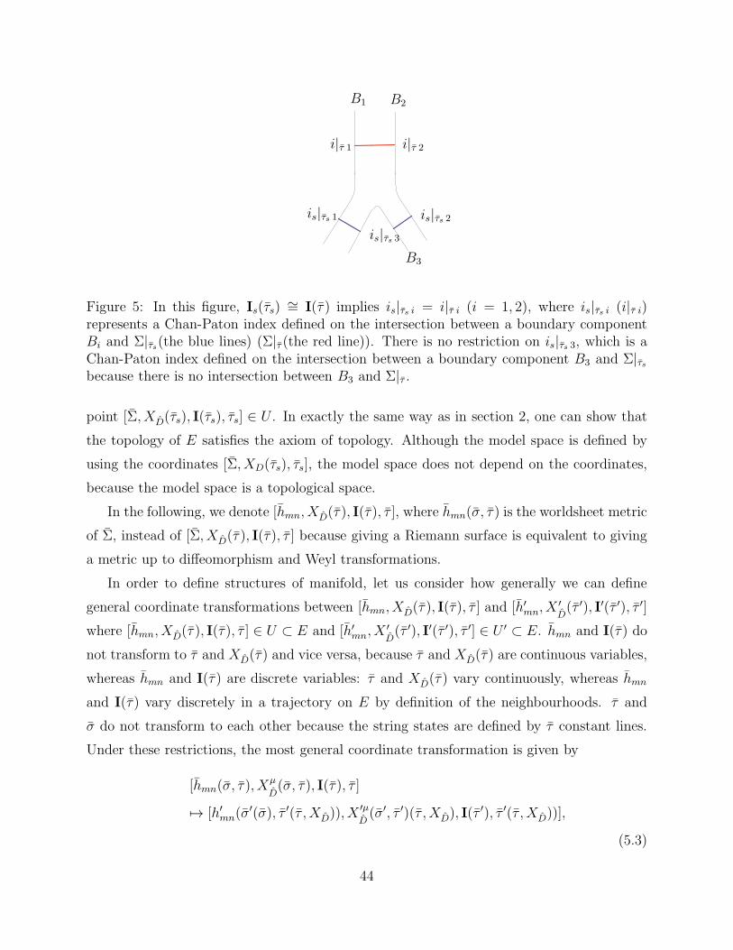
Figure 5: In this figure, Is(τs) ∼= I(τ ) implies is|τs i = i|τ i (i = 1, 2), where is|τs i (i|τ i)represents a Chan-Paton index defined on the intersection between a boundary componentBi and Σ|τs(the blue lines) (Σ|τ (the red line)). There is no restriction on is|τs 3, which is aChan-Paton index defined on the intersection between a boundary component B3 and Σ|τsbecause there is no intersection between B3 and Σ|τ .
point [Σ, XD(τs), I(τs), τs] ∈ U . In exactly the same way as in section 2, one can show that
the topology of E satisfies the axiom of topology. Although the model space is defined by
using the coordinates [Σ, XD(τs), τs], the model space does not depend on the coordinates,
because the model space is a topological space.
In the following, we denote [hmn, XD(τ ), I(τ), τ ], where hmn(σ, τ ) is the worldsheet metric
of Σ, instead of [Σ, XD(τ ), I(τ), τ ] because giving a Riemann surface is equivalent to giving
a metric up to diffeomorphism and Weyl transformations.
In order to define structures of manifold, let us consider how generally we can define
general coordinate transformations between [hmn, XD(τ ), I(τ), τ ] and [h′mn, X′D(τ ′), I′(τ ′), τ ′]
where [hmn, XD(τ ), I(τ), τ ] ∈ U ⊂ E and [h′mn, X′D(τ ′), I′(τ ′), τ ′] ∈ U ′ ⊂ E. hmn and I(τ) do
not transform to τ and XD(τ) and vice versa, because τ and XD(τ) are continuous variables,
whereas hmn and I(τ) are discrete variables: τ and XD(τ ) vary continuously, whereas hmn
and I(τ) vary discretely in a trajectory on E by definition of the neighbourhoods. τ and
σ do not transform to each other because the string states are defined by τ constant lines.
Under these restrictions, the most general coordinate transformation is given by
[hmn(σ, τ), Xµ
D(σ, τ), I(τ), τ ]
7→ [h′mn(σ′(σ), τ ′(τ , XD)), X
′µD(σ′, τ ′)(τ , XD), I(τ
′), τ ′(τ , XD))],
(5.3)
44
where hmn 7→ h′mn represents a world-sheet diffeomorphism transformation16. X′µ
D(τ , XD(τ ))
and τ ′(τ , XD(τ)) are functionals of τ and XD(τ ). µ = 0, 1, · · ·d−1. Here, we consider all the
manifolds which are constructed by patching open sets of the model space E by the general
coordinate transformations (5.3) and call them string manifolds M.
Here, we give an example of string manifolds: MD := [Σ, xD(τ), I(τ), τ ], where Drepresents a target metric Gµν , O-planes and D-bundles with gauge connections where all
the other backgrounds are turned off except for Gµν . xD(τ ) : Σ|τ → M , where the image of
the embedding function xD(τ) has a metric: ds2 = dxµD(τ , σ)dxνD(τ , σ)Gµν(xD(τ , σ)).
We will show that MD has a structure of manifold, that is there exists a general co-
ordinate transformation between the sufficiently small neighbourhood around an arbitrary
point [Σ, xsD(τs), Is(τs), τs] ∈ MD and an open set of E. There exists a general coordinate
transformation XD(xD) that satisfies ds2 = dxµDdx
νDGµν(xD) = dXµ
DdXν
Dηµν on an arbitrary
point xD in the ǫσ open neighbourhood around xsD(τs, σ) ∈ M , if ǫσ is sufficiently small.
An arbitrary point [Σ, xD(τ), I(τ), τ ] in the ǫ := inf0≦σ<2π ǫσ open neighbourhood around
of Σ are oriented open-closed worldsheets with punctures. First of all, we define global
coordinates on the double covers Σc of Σ in the same way as in section 4. The real part of
the global coordinates τ remains on Σ because ρ is an anti-holomorphic involution. If ρ maps
a puncture to another puncture on Σc, the superdiscs around the punctures are identified
and give a superdisk Di around a closed puncture P i on Σ. On the other hand, if ρ maps
a puncture to itself on Σc, the superdisk around the puncture is identified with itself and
gives an upper half superdisk Dj around an open puncture P j on Σ. The σ regions around
P i and P j are 2πf i and πf j, respectively where∑n
i=1 2fi +∑m
j=1 fj = 0. τ = −∞ at P i
and P j with negative f i and f j, respectively, whereas τ = ∞ at P i and P j with positive f i
and f j, respectively. In order to define the above global time uniquely, we fix the σ regions
2πf i and πf j around P i and P j, respectively in exactly the same way as in section 5.
Thus, under a superconformal transformation, one obtains Σ that has even coordinates
composed of the global time τ and the position σ, and Σred is canonically defined. Because
Σ can be a moduli of oriented open-closed superstring worldsheets with open and closed
punctures, any two-dimensional oriented open-closed super Riemannian manifold with open
and closed punctures Σ can be obtained by Σ = ψ(Σ) where ψ is a superdiffeomorphism
times super Weyl transformation.
Next, we will define the model space E. Here we fix not only a d-dimensional Euclidean
space Rd but also backgrounds except for the metric, that consist of a NS-NS B-field, a
dilaton, R-R fields 18, a set of submanifolds L in Rd, N dimensional vector bundles E with
18X
DTdo not depend on the R-R backgrounds because strings do not couple with them. However, open
sets of the model space need to possess the R-R backgrounds (We may writeE :=⋃
DT[Σ,X
DT, I(τ ), τ ]
DT.)
in order that D-brane states in the Hilbert space defined on the open sets couple with the R-R backgrounds.
50
gauge connections on them, which we call D-submanifolds and D-bundles, respectively, and
consistent configurations of O-planes.
We consider a state (Σ,XDT(τs), I(τs), τs) determined by a τ = τs constant hypersurface.
XDT(τs) : Σ|τs → Rd is an arbitrary map that maps a boundary component of the reduced
space into a D-submanifold. DT represents the above fixed quantities, where T runs IIA,
IIB and I. The IIA GSO projection is attached for T = IIA, and the IIB GSO projection is
attached for T = IIB and I. Ω projection is imposed and 32 D9-submanifolds are fixed for
T = I. We can define the worldsheet fermion numbers of states in a Hilbert space because
the states consist of the fields over the local coordinates Xµ
DT(τs) = Xµ + θαψµα + 1
2θ2F µ,
where µ = 0, 1, · · ·d−1, ψµα is a Majorana fermion and F µ is an auxiliary field. We abbreviate
DT and (τs) of Xµ, ψµα and F µ. We define the Hilbert space in these coordinates by the
states only with eπiF = 1 and eπiF = (−1)α for T = IIA and eπiF = eπiF = 1 for T =
IIB and I, where F and F are left- and right-handed fermion numbers respectively, and α
is 1 or 0 when the right-handed fermion is periodic (R sector) or anti-periodic (NS sector),
respectively.
I(τs) = (i|τs 1, · · · , i|τs k, · · · , i|τs b|τs ) represents a set of the Chan-Paton indices where
i|τs k represents a Chan-Paton index on the k-th intersection between Σ|τs and boundary
components on Σ. i|τs k runs from 1 to Nk that represents the dimension of the D-bundle
where the k-th intersection maps. An open string that has Chan-Paton indices (i|τs k−1, i|τs k)is represented by a part of Σ|τs that is surrounded by the k−1- and k-th intersections, whose
σ coordinates are represented by σk−1 and σk, respectively. The zero mode and the boundary
conditions on σk of Xµ are determined by the background including the D-submanifolds L
and the gauge connections.
Σ is a union of N± supercylinders with radii fi and M± superstrips with width πf j
at τ ≃ ±∞. Thus, we define a superstring state as an equivalence class [Σ,XDT(τs ≃
±∞), I(τs ≃ ±∞), τs ≃ ±∞] by a relation (Σ,XDT(τs ≃ ±∞), I(τs ≃ ±∞), τs ≃ ±∞) ∼
(Σ′,X′DT
(τs ≃ ±∞), I′(τs ≃ ±∞), τs ≃ ±∞) if N± = N ′±, M± = M ′
±, fi = f ′i, f j = f ′j ,
I(τs ≃ ±∞) = I′(τs ≃ ±∞), XDT(τs ≃ ±∞) = X′
DT(τs ≃ ±∞), and the corresponding
supercylinders and superstrips are the same type (NS-NS, NS-R, R-NS, or R-R) and (NS or
R), respectively as in Fig. 1. [Σ,XDT(τs), I(τs), τs] represent many-body states of open and
closed superstrings in Rd as in Fig. 2, because the reduced space of Σ|τs is S1 × · · · × S1 ×
51
I1 × · · · × I1 where I1 represents a line segment, and XDT(τs) : Σ|τs → Rd. We define the
model space E such that E :=⋃
DT[Σ,XDT
(τ), I(τ), τ ] where disjoint unions are taken
over all the backgrounds DT except for the metric.
Here, we will define topologies of E. An ǫ-open neighbourhood of [Σ,Xs DT(τs), Is(τs), τs]
Is(τs) ∼= I(τ) means that a Chan-Paton index on the intersection between Σ|τs and a
boundary component on Σ equals a Chan-Paton index on the intersection between Σ|τand the boundary component, excepting that the corresponding intersection does not ex-
ist. For example, see Fig. 5. U([Σ,XDT(τs ≃ ±∞), I(τs ≃ ±∞), τs ≃ ±∞], ǫ) =
U([Σ′,X′DT
(τs ≃ ±∞), I′(τs ≃ ±∞), τs ≃ ±∞], ǫ) consistently if N± = N ′±, M± = M ′
±,
f i = f ′i, f j = f ′j, the corresponding supercylinders and superstrips are the same type
(NS-NS, NS-R, R-NS, or R-R) and (NS or R), respectively, I(τs ≃ ±∞) = I′(τs ≃ ±∞),
XDT(τs ≃ ±∞) = X′
DT(τs ≃ ±∞), and ǫ is small enough, because the τ = τs constant
line traverses only propagators overlapped by Σ and Σ′. U is defined to be an open set
of E if there exists ǫ such that U([Σ,XDT(τs), I(τs), τs], ǫ) ⊂ U for an arbitrary point
[Σ,XDT(τs), I(τs), τs] ∈ U . In exactly the same way as in section 2, one can show that
the topology of E satisfies the axiom of topology. Although the model space is defined by
using the coordinates [Σ,XDT(τ ), I(τ), τ ], the model space does not depend on the coordi-
nates, because the model space is a topological space.
In the following, we denote [E AM (σ, τ , θα),XDT
(τ ), I(τ), τ ], where E AM (σ, τ , θα) (M =
(m,α), A = (q, a), m, q = 0, 1, α, a = 1, 2) is the worldsheet super vierbein on Σ, instead of
52
[Σ,XDT(τ), I(τ), τ ] because giving a super Riemann surface is equivalent to giving a super
vierbein up to super diffeomorphism and super Weyl transformations.
In order to define structures of manifold, let us consider how generally we can define gen-
eral coordinate transformations between [E AM ,XDT
(τ), I(τ), τ ] and [E′ AM ,X′
DT(τ ′), I′(τ ′), τ ′]
where [E AM ,XDT
(τ), I(τ), τ ] ∈ U ⊂ E and [E′ AM ,X′
DT(τ ′), I′(τ ′), τ ′] ∈ U ′ ⊂ E. E A
M and
I(τ) do not transform to τ and XDT(τ) and vice versa, because τ and XDT
(τ) are continuous
variables, whereas E AM and I(τ) are discrete variables: τ and XDT
(τ) vary continuously,
whereas E AM and I(τ) vary discretely in a trajectory on E by definition of the neighbour-
hoods. τ does not transform to σ and θ and vice versa, because the superstring states are
defined by τ constant hypersurfaces. Under these restrictions, the most general coordinate
transformation is given by
[E AM (σ, τ , θα),Xµ
DT(σ, τ , θα), I(τ), τ ]
7→ [E′ AM (σ′(σ, θ), τ ′, θ
′α(σ, θ)),X′µ
DT(σ′, τ ′, θ
′α)(τ ,XDT(τ )), I(τ ′), τ ′(τ ,XDT
(τ ))],
(6.3)
where E AM 7→ E
′ AM represents a world-sheet superdiffeomorphism transformation19. X
′µ
DT(τ ,XDT
(τ))
and τ ′(τ ,XDT(τ )) are functionals of τ andXDT
(τ ). Here, we consider all the manifolds which
are constructed by patching open sets of the model space E by general coordinate transfor-
mations (6.3) and call them superstring manifolds M.
Here, we give an example of superstring manifolds: MDT:= [Σ,xDT
(τ ), I(τ), τ ], whereDT represents a target metric Gµν , O-planes and D-bundles with gauge connections where
all the other backgrounds are turned off except for Gµν , and a type of the GSO projection.
xDT(τ) : Σ|τ → M , where x
µDT
(τ) = xµ + θαψµα + 12θ2fµ. The image of the bosonic part of
the embedding function, x(τ ) has a metric: ds2 = dxµ(τ , σ)dxν(τ , σ)Gµν(x(τ , σ)).
We will show that MDThas a structure of manifold, that is there exists a general co-
ordinate transformation between the sufficiently small neighbourhood around an arbitrary
point [Σ,xsDT(τs), Is(τs), τs] ∈ MDT
and an open set of E. There exists a general coordi-
nate transformation Xµ(x) that satisfies ds2 = dxµdxνGµν(x) = dXµdXνηµν on an arbitrary
point x in the ǫσ open neighbourhood around xs(τs, σ) ∈ M , if ǫσ is sufficiently small.
19 We extend the model space from E = [E AM (σ, τ , θα),Xµ
DT
(σ, τ , θα), I(τ ), τ ] to E =
[E′ AM (σ′, τ ′, θ
′α),X′µ
DT
(σ′, τ ′, θ′α), I(τ ′), τ ′] by including the points generated by the superdiffeomor-
phisms σ 7→ σ′(σ, θ), θα 7→ θ′α(σ, θ), and τ 7→ τ ′(τ ).
53
An arbitrary point [Σ,xDT(τ), I(τ), τ ] in the ǫ := inf0≦σ<2π ǫσ open neighbourhood around
λDT(τ , σ), there exist vector bundles for 0 ≦ σ < 2π and θ, and its section XDT
(τ) and
λDT(τ). xDT
(τ) and XDT(τ ) satisfy (8.8) on each σ, that is XDT
(τ) : Σ|τ → Rd. Therefore,
64
there exists a general coordinate transformation between the sufficiently small neighbour-
hood around an arbitrary point [Σ,xsDT(τs), λsDT
(τs), τs] ∈ MDTand an open set of E:
[Σ,xDT(τ), λDT
(τ ), τ ] 7→ [Σ,XDT(τ), λDT
(τ), τ ].
By definition of the ǫ-open neighbourhood, arbitrary two superstring states on a con-
nected heterotic super Riemann surface are connected continuously. Thus, there is an one-
to-one correspondence between a heterotic super Riemann surface with punctures in M and
a curve parametrized by τ from τ = −∞ to τ = ∞ on MDT. That is, curves that repre-
sent asymptotic processes on MDTreproduce the right moduli space of the heterotic super
Riemann surfaces in the target manifold.
By a general curve parametrized by t on MDT, superstring states on different heterotic
super Riemann surfaces that have even different genera, can be connected continuously,
for example see Fig. 3, whereas different super Riemann surfaces that have different gen-
era cannot be connected continuously in the moduli space of the heterotic super Riemann
surfaces in the target space. Therefore, the superstring geometry is expected to possess
non-perturbative effects.
In the following, instead of the fermionic coordinate λADT
(σ, τ), we use a bosonic coordi-
nate XA
LDT(σ, τ , θ−) := θ−λA
DT(σ, τ) where θ− has the opposite chirality to θ+.
The tangent space is spanned by ∂∂X
µ
DT(σ,τ ,θ)
, ∂
∂XA
LDT(σ,τ ,θ−)
and ∂∂τ
as one can see from the
ǫ-open neighbourhood (8.3). We should note that ∂∂E A
M
cannot be a part of basis that span
the tangent space because E AM is just a discrete variable in E. The indices of ∂
∂Xµ
DT(σ,τ ,θ)
and ∂∂XA
LDT(σ,τ ,θ−)
can be (µ σ θ) and (A σ θ−), where µ = 0, 1, · · · , d − 1 and A = 1, · · ·32,respectively. Then, let us define a summation over σ and θ that is invariant under (σ, θ) 7→(σ′(σ, θ), θ′(σ, θ)) and transformed as a scalar under τ 7→ τ ′(τ ,XDT
(τ ),XLDT(τ)). First,
∫
dτ∫
dσdθE(σ, τ , θ) is invariant under (σ, τ , θ) 7→ (σ′(σ, θ), τ ′(τ ,XDT(τ),XLDT
(τ)), θ′(σ, θ)),
where E(σ, τ , θ) is the superdeterminant of E AM (σ, τ , θ). A super analogue of the lapse func-
tion, 1√E0
AE0Atransforms as an one-dimensional vector in the τ direction:
∫
dτ 1√E0
AE0Ais in-
variant under τ 7→ τ ′(τ ,XDT(τ ),XLDT
(τ)) and transformed as a superscalar under (σ, θ) 7→(σ′(σ, θ), θ′(σ, θ)). Therefore,
∫
dσdθE(σ, τ , θ), where E(σ, τ , θ) :=√
E0AE
0AE(σ, τ , θ), is
transformed as a scalar under τ 7→ τ ′(τ ,XDT(τ),XLDT
(τ )) and invariant under (σ, θ) 7→(σ′(σ, θ), θ′(σ, θ)). The summation over σ and θ− is defined by
∫
dσdθ−e(σ, τ), where
e :=√
hσσ. This summation is also invariant under (σ, θ) 7→ (σ′(σ, θ), θ′(σ, θ)), where
65
θ− is not transformed, and transformed as a scalar under τ 7→ τ ′(τ ,XDT(τ ),XLDT
(τ)).
Riemannian heterotic superstring manifold is obtained by defining a metric, which is a
section of an inner product on the tangent space. The general form of a metric is given by
ds2(E,XDT(τ),XLDT
(τ), τ)
= G(E,XDT(τ ),XLDT
(τ), τ)dd(dτ)2
+2dτ
∫
dσdθE∑
µ
G(E,XDT(τ ),XLDT
(τ), τ)d (µσθ)dXµ
DT(σ, τ , θ)
+2dτ
∫
dσdθ−e∑
A
G(E,XDT(τ),XLDT
(τ ), τ)d (Aσθ−)dXA
LDT(σ, τ , θ−)
+
∫
dσdθE
∫
dσ′dθ′E′∑
µ,µ′
G(E,XDT(τ ),XLDT
(τ), τ) (µσθ) (µ′σ′ θ′)dXµ
DT(σ, τ , θ)dXµ′
DT(σ′, τ , θ′)
+
∫
dσdθE
∫
dσ′dθ−e′∑
µ,A
G(E,XDT(τ),XLDT
(τ), τ ) (µσθ) (Aσ′θ−)dXµ
DT(σ, τ , θ)dXA
LDT(σ′, τ , θ−)
+
∫
dσdθ−e
∫
dσ′dθ′−e′
∑
A,A′
G(E,XDT(τ ),XLDT
(τ), τ) (Aσθ−) (A′σ′θ′−)
dXA
LDT(σ, τ , θ−)dXA′
LDT(σ′, τ , θ
′−).
(8.9)
We summarize the vectors as dXI
DT(I = d, (µσθ), (Aσθ−)), where dXd
DT:= dτ , dX
(µσθ)
DT:=
dXµ
DT(σ, τ , θ) and dX
(Aσθ−)
DT:= dXA
LDT(σ, τ , θ−). Then, the components of the metric are
summarized asGIJ(E,XDT(τ),XLDT
(τ), τ ). The inverse of the metricGIJ(E,XDT(τ ),XLDT
(τ), τ)
is defined by GIJGJK = GKJGJI = δK
I, where δdd = 1, δµ
′σ′θ′
µσθ= 1
Eδµ
′
µ δ(σ − σ′)δ(θ − θ′) and
δA′σ′θ
′−
Aσθ−= 1
eδA
′
A δ(σ− σ′)δ(θ−− θ′−). The components of the Riemannian curvature tensor are
given by RI
JKLin the basis ∂
∂XI
DT
. The Ricci tensor is RIJ := RK
IKJand the scalar curvature
is R := GIJRIJ. The volume is vol =√G, where G = det(GIJ).
By using these geometrical objects, we define a superstring theory non-perturbatively as
Z =
∫
DGDAe−S, (8.10)
where
S =1
GN
∫
DEDXDT(τ)DXLDT
(τ )Dτ√G(−R +
1
4GNG
I1I2GJ1J2FI1J1FI2J2). (8.11)
As an example of sets of fields on the superstring manifolds, we consider the metric and an
u(1) gauge field AI whose field strength is given by FIJ. The path integral is canonically
66
defined by summing over the metrics and gauge fields on M. By definition, the theory is
background independent. DE is the invariant measure of the super vierbeins E AM on the
two-dimensional super Riemannian manifolds Σ. E AM and E A
M are related to each others
by the super diffeomorphism and super Weyl transformations.
Under
(τ ,XDT(τ ),XLDT
(τ))
7→ (τ ′(τ ,XDT(τ),XLDT
(τ )),X′DT
(τ ′)(τ ,XDT(τ),XLDT
(τ)),X′LDT
(τ ′)(τ ,XDT(τ ),XLDT
(τ))),
(8.12)
GIJ(E,XDT(τ),XLDT
(τ ), τ) and AI(E,XDT(τ ),XLDT
(τ), τ) are transformed as a symmetric
tensor and a vector, respectively and the action is manifestly invariant.
We define GIJ(E,XDT(τ ),XLDT
(τ), τ) and AI(E,XDT(τ),XLDT
(τ ), τ) so as to transform
as scalars under E AM (σ, τ , θ) 7→ E
′ AM (σ′(σ, θ), τ , θ
′
(σ, θ)). Under (σ, θ) superdiffeomor-
phisms: (σ, θ) 7→ (σ′(σ, θ), θ′(σ, θ)), which are equivalent to
[E AM (σ, τ , θ),Xµ
DT(σ, τ , θ),XA
LDT(σ, τ , θ−), τ ]
7→ [E′ AM (σ′(σ, θ), τ , θ′(σ, θ)),X
′µ
DT(σ′(σ, θ), τ , θ′(σ, θ))(XDT
(τ)),X′A
LDT(σ′(σ, θ), τ , θ−)(XLDT
(τ )), τ ]
= [E′ AM (σ′(σ, θ), τ , θ′(σ, θ)),Xµ
DT(σ, τ , θ),XA
LDT(σ, τ , θ−), τ ], (8.13)
Gd (Aσθ−) is transformed as a scalar;
G′d (Aσ′ θ−)(E
′,X′DT
(τ),X′LDT
(τ ), τ) = G′d (Aσ′θ−)(E,X
′DT
(τ ),X′LDT
(τ ), τ)
=∂XI
DT(τ)
∂X′d
DT(τ)
∂XJ
DT(τ )
∂X′(Aσ′ θ−)
DT(τ )
GIJ(E,XDT(τ ),XLDT
(τ), τ)
=∂XI
DT(τ)
∂Xd
DT(τ)
∂XJ
DT(τ)
∂X(Aσθ−)
DT(τ )
GIJ(E,XDT(τ),XLDT
(τ ), τ)
= Gd (Aσθ−)(E,XDT(τ),XLDT
(τ ), τ), (8.14)
67
because (8.12) and (8.13). In the same way, the other fields are also transformed as
G′dd(E
′,X′DT
(τ),X′LDT
(τ ), τ) = Gdd(E,XDT(τ),XLDT
(τ ), τ)
G′d (µσ′ θ′)(E
′,X′DT
(τ),X′LDT
(τ ), τ) = Gd (µσθ)(E,XDT(τ ),XLDT
(τ), τ)
G′(µσ′ θ′) (νρ′ ˜θ′)
(E′,X′DT
(τ),X′LDT
(τ ), τ) = G(µσθ) (νρ ˜θ)
(E,XDT(τ ),XLDT
(τ), τ)
G′(µσ′θ′) (Aρ′ ˜θ−)
(E′,X′DT
(τ),X′LDT
(τ ), τ) = G(µσθ) (Aρ ˜θ−)
(E,XDT(τ ),XLDT
(τ), τ)
G′(Aσ′θ−) (Bρ′ ˜θ−)
(E′,X′DT
(τ),X′LDT
(τ ), τ) = G(Aσθ−) (Bρ ˜θ−)
(E,XDT(τ),XLDT
(τ), τ )
A′d(E
′,X′DT
(τ),X′LDT
(τ ), τ) = Ad(E,XDT(τ),XLDT
(τ ), τ)
A′(µσ′ θ′)(E
′,X′DT
(τ),X′LDT
(τ ), τ) = A(µσθ)(E,XDT(τ),XLDT
(τ), τ)
A′(Aσ′ θ−)(E
′,X′DT
(τ),X′LDT
(τ ), τ) = A(Aσθ−)(E,XDT(τ),XLDT
(τ ), τ). (8.15)
Thus, the action is invariant under the (σ, θ) superdiffeomorphisms, because
∫
dσ′dθ′E′(σ′, τ , θ′) =
∫
dσdθE(σ, τ , θ)∫
dσ′dθ−e′(σ′, τ) =
∫
dσdθ−e(σ, τ) (8.16)
Therefore, GIJ(E,XDT(τ ),XLDT
(τ), τ) and AI(E,XDT(τ ),XLDT
(τ), τ) are transformed co-
variantly and the action (8.11) is invariant under the diffeomorphisms (8.5) including the
(σ, θ) superdiffeomorphisms, whose infinitesimal transformations are given by
σξ = σ − i
2ξθ
θξ(σ) = θ + ξ(σ), (8.17)
(8.17) are dimensional reductions in τ direction of the two-dimensional N = (0, 1) local
supersymmetry infinitesimal transformations. The number of supercharges
ξQ = ξ(∂
∂θ− i
2θ∂
∂σ) (8.18)
of the transformations is the same as of the two-dimensional ones. The supersymmetry
algebra closes in a field-independent sense as in ordinary supergravities.
68
The background that represents a perturbative vacuum is given by
ds2
= 2ζρ(h)N2(XDT(τ ),XLDT
(τ))(dXd
DT)2
+
∫
dσdθE
∫
dσ′dθ′E′N2
2−D (XDT(τ ),XLDT
(τ))e2(σ, τ )E(σ, τ , θ)
√
h(σ, τ)δ(µσθ)(µ′σ′ θ′)dX
(µσθ)
DTdX
(µ′σ′θ′)
DT
+
∫
dσdθ−e
∫
dσ′dθ′−e′N
22−D (XDT
(τ),XLDT(τ))
e3(σ, τ )√
h(σ, τ)δ(Aσθ−)(A′σ′ θ
′−)dX(Aσθ−)
LDTdX
(A′σ′θ′−)
LDT,
Ad = i
√
2− 2D
2−D
√
2ζρ(h)√GN
N(XDT(τ),XLDT
(τ)), A(µσθ) = 0, A(Aσθ−) = 0, (8.19)
on MDTwhere we fix the target metric to ηµµ′ . ρ(h) :=
14π
∫
dσ√hRh, where Rh is the scalar
curvature of hmn. D is a volume of the index (µσθ) and (Aσθ−): D :=∫
dσdθEδ(µσθ)(µσθ) +∫
dσdθ−eδ(Aσθ−)(Aσθ−) = (d+32)∫
dσdθδ(σ−σ)δ(θ−θ). N(XDT(τ ),XLDT
(τ )) = 11+v(X
DT(τ ),X
LDT(τ))
,
where
v(XDT(τ),XLDT
(τ )) =α√d− 1
∫
dσdθe
√E
(h)14
ǫµνXµ
DT(τ )
√
∂zDθXν
DT(τ)
+β√31
∫
dσdθ−e
√EL
(h)14
ǫABXA
LDT(τ)
√
∂zDθ−XB
LDT(τ ). (8.20)
∂zDθ is a τ independent operator that satisfies∫
dτdσdθE−1
2Xµ
DT(τ)∂zDθXDTµ
(τ)
=
∫
dτdσ√
h1
2
(
e−2(∂σXµ)2 + E1
zψµχz∂σXµ + ψµE1
z∂σψµ
−1
4n2E0
zψµχzE
0zψµχz + nσ∂σXµE
0zψ
µχz
)
, (8.21)
where Emq and χz are a vierbein and a gravitino in the two dimensions, respectively. On the
other hand, the ordinary super covariant derivative Dθ = ∂θ + θ∂z satisfies [42–44]∫
dτdσdθE−1
2Xµ
DT(τ)∂zDθXDTµ
(τ )
=
∫
dτdσ√
h1
2(hmn∂mX
µ∂nXµ + ψµEmz ∂mψµ + Em
z ∂mXµψµχz). (8.22)
EL is the chiral conjugate of E. ∂z := E1z∂σ and Dθ− := ∂θ− + θ−E1
z∂σ satisfy∫
dτdσdθ−EL−1
2XA
LDT(τ)∂zDθ−XLDT A
(τ ) =
∫
dτdσ√
h1
2λAE1
z∂σλA, (8.23)
69
whereas the ordinary super covariant derivative Dθ− = ∂θ− + θ−∂z satisfies
∫
dτdσdθ−EL−1
2XA
LDT(τ )∂zDθ−XLDT A
(τ) =
∫
dτdσ√
h1
2λAEm
z ∂mλA. (8.24)
The inverse of the metric is given by
Gdd =1
2ζρ
1
N2
G(µσθ) (µ′σ′θ′) = N−2
2−D
√h
e2Eδ(µσθ)(µ′σ′θ′)
G(Aσθ−) (A′σ′θ′−) = N
−22−D
√h
e3δ(Aσθ−)(A′σ′θ
′−), (8.25)
where the other components are zero. From the metric, we obtain
√
G = N2
2−D
√
2ζρ exp(
∫
dσdθEδ(µσθ) (µσθ) lne2E√h+
∫
dσdθ−eδ(Aσθ−) (Aσθ−) lne3√h)
Rdd = −2ζρN−2
2−D
(
∫
dσdθ
√h
e2∂(µσθ)N∂(µσθ)N +
∫
dσdθ−√h
e2∂(Aσθ−)N∂(Aσθ−)N
)
R(µσθ) (µ′σ′θ′) =D− 1
2−DN−2∂(µσθ)N∂(µ′σ′θ′)N
+1
D− 2N−2
(
∫
dσ′′dθ′′√h′′
e′′2∂(µ′′σ′′ θ′′)N∂(µ′′σ′′ θ′′)N
+
∫
dσ′′dθ′′−
√h′′
e′′2∂(A′′σ′′θ
′′−)N∂(A′′σ′′ θ′′−)N
)
Ee2√hδ(µσθ) (µ′σ′θ′)
R(Aσθ−) (A′σ′θ′−) =
D− 1
2−DN−2∂(Aσθ−)N∂(A′σ′θ
′−)N
+1
D− 2N−2
(
∫
dσ′′dθ′′√h′′
e′′2∂(µ′′σ′′ θ′′)N∂(µ′′σ′′ θ′′)N
+
∫
dσ′′dθ′′−
√h′′
e′′2∂(A′′σ′′θ
′′−)N∂(A′′σ′′ θ′′−)N
)
e3√hδ(Aσθ−) (A′σ′θ
′−)
R =D− 3
2−DN
2D−62−D
(
∫
dσdθ
√h
e2∂(µσθ)N∂(µσθ)N +
∫
dσdθ−√h
e2∂(Aσθ−)N∂(Aσθ−)N
)
.
(8.26)
By using these quantities, one can show that the background (8.19) is a classical solution to
the equations of motion of (8.11). We also need to use the fact that v(XDT(τ),XLDT
(τ)) is
70
a harmonic function with respect to X(µσθ)
DT(τ ) and X
(Aσθ−)
LDT(τ). Actually, ∂(µσθ)∂(µσθ)v =
∂(Aσθ−)∂(Aσθ−)v = 0. In these calculations, we should note that E AM , τ , X
µ
DT(τ ) and
XA
LDT(τ ) are all independent, and thus ∂
∂τis an explicit derivative on functions over the
superstring manifolds, especially, ∂∂τE AM = 0, ∂
∂τXµ
DT(τ ) = 0 and ∂
∂τXA
LDT(τ) = 0. Because
the equations of motion are differential equations with respect to τ , Xµ
DT(τ) and XA
LDT(τ ),
E AM is a constant in the solution (8.19) to the differential equations. The dependence
of E AM on the background (8.19) is uniquely determined by the consistency of the quan-
tum theory of the fluctuations around the background. Actually, we will find that all the
perturbative superstring amplitudes are derived.
Let us consider fluctuations around the background (8.19), GIJ = GIJ + GIJ and AI =
AI + AI. Here we fix the charts, where we choose T=SO(32) or E8 ×E8. The action (8.11)
up to the quadratic order is given by,
S =1
GN
∫
DEDXDT(τ )DXLDT
(τ)Dτ√
G(
−R +1
4F ′IJF ′IJ
+1
4∇IGJK∇IGJK − 1
4∇IG∇IG+
1
2∇IGIJ∇JG− 1
2∇IGIJ∇KG
JK
−1
4(−R +
1
4F ′KLF ′KL)(GIJG
IJ − 1
2G2) + (−1
2RI
J+
1
2F ′IKF ′
JK)GILG
JL
+(1
2RIJ − 1
4F ′IKF ′J
K)GIJG+ (−1
2RIJKL +
1
4F ′IJF ′KL)GIKGJL
+1
4GN FIJF
IJ +√
GN(1
4F
′IJFIJG− F
′IJFIKG
K
J))
, (8.27)
where F ′IJ
:=√GN FIJ is independent of GN . G := GIJGIJ. There is no first order term
because the background satisfies the equations of motion. If we take GN → 0, we obtain
S ′ =1
GN
∫
DEDXDT(τ)DXLDT
(τ )Dτ√
G(
−R +1
4F ′IJF ′IJ
+1
4∇IGJK∇IGJK − 1
4∇IG∇IG+
1
2∇IGIJ∇JG− 1
2∇IGIJ∇KG
JK
−1
4(−R +
1
4F ′KLF ′KL)(GIJG
IJ − 1
2G2) + (−1
2RI
J+
1
2F ′IKF ′
JK)GILG
JL
+(1
2RIJ − 1
4F ′IKF ′J
K)GIJG+ (−1
2RIJKL +
1
4F ′IJF ′KL)GIKGJL
)
, (8.28)
where the fluctuation of the gauge field is suppressed. In order to fix the gauge symmetry
(8.12), we take the harmonic gauge. If we add the gauge fixing term
Sfix =1
GN
∫
DEDXDT(τ )DXLDT
(τ)Dτ√
G1
2
(
∇J(GIJ −1
2GIJG)
)2
, (8.29)
71
we obtain
S ′ + Sfix =1
GN
∫
DEDXDT(τ)DXLDT
(τ)Dτ√
G(
−R +1
4F ′IJF ′IJ
+1
4∇IGJK∇IGJK − 1
8∇IG∇IG
−1
4(−R +
1
4F ′KLF ′KL)(GIJG
IJ − 1
2G2) + (−1
2RI
J+
1
2F ′IKF ′
JK)GILG
JL
+(1
2RIJ − 1
4F ′IKF ′J
K)GIJG+ (−1
2RIJKL +
1
4F ′IJF ′KL)GIKGJL
)
. (8.30)
In order to obtain perturbative string amplitudes, we perform a derivative expansion of
GIJ,
GIJ → 1
αGIJ
∂KGIJ → ∂KGIJ
∂K∂LGIJ → α∂K∂LGIJ, (8.31)
and take
α = β → 0, (8.32)
where α and β are arbitrary constants in the solution (8.19). We normalize the fields as
HIJ := ZIJGIJ, where ZIJ := 1√GNG
14 (aIaJ)
− 12 . aI represent the background metric as
GIJ = aIδIJ, where ad = 2ζρ, a(µσθ) =e2E√hand a(Aσθ−) =
e3√h. Then, (8.30) with appropriate
boundary conditions reduces to
S ′ + Sfix → S0 + S2, (8.33)
where
S0 =1
GN
∫
DEDXDT(τ )DXLDT
(τ )Dτ√
G(
−R +1
4F ′IJF ′IJ
)
, (8.34)
and
S2 =
∫
DEDXDT(τ)DXLDT
(τ )Dτ 18HIJHIJ;KLHKL. (8.35)
In the same way as in section 3, a part of the action
∫
DEDXDT(τ)DXLDT
(τ )Dτ 14
∫ 2π
0
dσdθH⊥d(µσθ)HH
⊥d(µσθ) (8.36)
with
72
H = −1
2
1
2ζρ(∂
∂τ)2 − 1
2
∫ 2π
0
dσ
∫
dθ
√h
e2(
∂
∂Xµ
DT(τ)
)2
−1
2
D2 − 9D+ 20
(2−D)2
(∫ 2π
0
dσ
∫
dθEXµ
DT(τ)∂zDθXDTµ
(τ)
+
∫ 2π
0
dσ
∫
dθ−ELXA
LDT(τ)∂zDθ−XLDT A
(τ )
)
(8.37)
decouples from the other modes. In (8.36), the term including ( ∂∂XA
LDT(τ)
)2 vanishes because
H⊥d(µσθ)
needs to be proportional to (XA
LDT(τ ))2 = (θ−λA
DT(τ))2 = 0 so as not to vanish.
In the following, we consider a sector that consists of local fluctuations in a sense of
strings as
HIJ =
∫ 2π
0
dσ′dθhIJ(Xµ
DT(τ , σ, θ)). (8.38)
Because we have
∫
dθ′
(
∂
∂Xµ
DT(τ , σ′, θ′)
)2
H⊥d(µσθ) =
(
∂
∂Xµ(τ , σ′)
)2
H⊥d(µσθ), (8.39)
as in section 4, (8.36) can be simplified with
H(−i ∂∂τ,−i1
e
∂
∂X,XDT
(τ ),XLDT(τ ), E)
=1
2
1
2ζρ(−i ∂
∂τ)2 +
∫
dσ√
h1
2(−i1
e
∂
∂X)2 −
∫
dσdθE1
2Xµ
DT(τ )∂zDθXDTµ
(τ )
−∫
dσdθ−EL1
2XA
LDT(τ )∂zDθ−XLDT A
(τ), (8.40)
where we have taken D → ∞. By adding to (8.36), a formula similar to the bosonic case
0 =
∫
DEDXDT(τ)DXLDT
(τ )Dτ 14
∫ 2π
0
dσ′dθ′H⊥d(µσ′ θ′)(
∫ 2π
0
dσnσ∂σXµ ∂
∂Xµ)H⊥
d(µσ′ θ′),
(8.41)
and
0 =
∫
DEDXDT(τ )DXLDT
(τ)Dτ 14
∫ 2π
0
dσ′dθ′H⊥d(µσ′ θ′)
∫ 2π
0
dσE−i2nχzE
0zψ
µ(−i1e
∂
∂Xµ)H⊥
d(µσ′ θ′),
(8.42)
73
we obtain (8.36) with
H(−i ∂∂τ,−i1
e
∂
∂X,XDT
(τ ), λDT(τ), E)
=1
2
1
2ζρ(−i ∂
∂τ)2 +
∫
dσ
(
√
h
(
1
2(−i1
e
∂
∂X)2 − i
2nχzE
0zψµ(−i
1
e
∂
∂X)
)
+ ienσ∂σXµ(−i1
e
∂
∂X)
)
−∫
dσdθE1
2Xµ
DT(τ )∂zDθXDTµ
(τ) +
∫
dσ√
h1
2λADT
(τ )E1z∂σλDTA
(τ), (8.43)
where we have used (8.23). (8.42) is true because the integrand of the right hand side is a
total derivative with respect to Xµ.
The propagator for H⊥d(µσθ)
;
∆F (E, τ ,XDT(τ ), λDT
(τ); E,′ τ ,′ X′DT
(τ ′), λ′DT
(τ ′))
= < H⊥d(µσθ)(E, τ ,XDT
(τ ), λDT(τ))H⊥
d(µσθ)(E,′ τ ,′ X′
DT(τ ′), λ′
DT(τ ′)) > (8.44)
satisfies
H(−i ∂∂τ,−i1
e
∂
∂X,XDT
(τ ), λDT(τ), E)∆F (E, τ ,XDT
(τ ), λDT(τ); E,′ τ ′,X′
DT(τ ′), λ′
DT(τ ′))
= δ(E− E′)δ(τ − τ ′)δ(XDT(τ)−X′
DT(τ ′))δ(λDT
(τ )− λ′DT
(τ ′)). (8.45)
In order to obtain a Schwinger representation of the propagator, we use the operator
formalism ( ˆE, ˆτ, XDT(ˆτ), λDT
(ˆτ)) of the first quantization. The eigen state for ( ˆE, ˆτ, X) is
given by |E, τ , X >. The conjugate momentum is written as (pE, pτ , pX). The Majorana
fermions ψµ and λADT
are self-conjugate. Renormalized operatorsˆψµ :=
√
E0z ψ
µ andˆλADT
:=√
E0z λ
A
DTsatisfy ˆψµ(σ), ˆψν(σ′) = 1
Eηµνδ(σ − σ′) and ˆλA
DT(σ),
ˆλBDT
(σ′) = 1EδABδ(σ − σ′),
respectively. By defining creation and annihilation operators for ψµ asˆψµ† := 1√
2(ˆψµ−i ˆψµ+ d
2 )
and ˆψµ := 1√2( ˆψµ+ i ˆψµ+
d2 ) where µ = 0, · · · d
2− 1, one obtains an algebra ˆψµ(σ), ˆψν†(σ′) =
1Eηµνδ(σ − σ′), ˆψµ(σ), ˆψν(σ′) = 0, and ˆψµ†(σ), ˆψν†(σ′) = 0. The vacuum |0 > for this
algebra is defined by ˆψµ(σ)|0 >= 0. The eigen state |ψ >, which satisfies ˆψµ(σ)|ψ >=
ψµ(σ)|ψ >, is given by e−ψ·ˆψ† |0 >= e−
∫dσEψµ(σ)
ˆψµ†(σ)|0 >. Then, the inner product is given
by < ψ|ψ′ >= eψ†·ψ′
, whereas the completeness relation is∫
Dψ†Dψ|ψ > e−ψ†·ψ < ψ| = 1.
The same is applied to λADT
(τ ).
Because (8.45) means that ∆F is an inverse of H , ∆F can be expressed by a matrix
74
element of the operator H−1 as
∆F (E, τ ,XDT(τ), λDT
(τ ); E,′ τ ,′ X′DT
(τ ′), λ′DT
(τ ′))
= < E, τ ,XDT(τ), λDT
(τ )|H−1(pτ , pX , XDT(τ ), λDT
(τ), ˆE)|E,′ τ ,′ X′DT
(τ ′), λ′DT
(τ ′) > .
(8.46)
(3.35) implies that
∆F (E, τ ,XDT(τ ), λDT
(τ); E,′ τ ,′ X′DT
(τ ′), λ′DT
(τ ′))
=
∫ ∞
0
dT < E, τ ,XDT(τ), λDT
(τ)|e−TH |E,′ τ ,′ X′DT
(τ ′), λ′DT
(τ ′) > . (8.47)
In order to define two-point correlation functions that is invariant under the general
coordinate transformations in the superstring geometry, we define in and out states as
||XDT i, λDT i
|Ef , ;Ei >in :=
∫
Ef
Ei
DE′|E,′ τ = −∞,XDT i, λDT i
>
< XDT f, λDT f
|Ef , ;Ei||out :=
∫
Ef
Ei
DE < E, τ = ∞,XDT f, λDT f
|, (8.48)
where Ei and Ef represent the super vierbeins of the supercylinders at τ = ±∞, respectively.
When we insert asymptotic states, we integrate out XDT f, XDT i
, λDT f, λDT i
, Ef and Ei in
the two-point correlation function for these states;
26The correlation function is zero if Ei and Ef of the in state do not coincide with those of the out states,because of the delta functions in the seventh line.
76
where E 0 = E′, τ0 = −∞, XDT 0 = XDT i, λDT 0 = λDT i
, EN+1 = E, τN+1 = ∞, XDTN+1 =
XDT f, and λDT N+1 = λDT f
. pX · ddtX =
∫
dσepµXddtXµ and ∆t = 1√
Nas in the bosonic
case. A trajectory of points [Σ,XDT(τ), λDT
(τ ), τ ] is necessarily continuous in MDTso that
the kernel < Ei+1, τi+1,XDT i+1(τi+1), λDT i+1(τi+1)|e−1NTiH |Ei, τi,XDT i
(τi), λDT i(τi) > in the
fourth line is non-zero when N → ∞. If we integrate out pτ (t) and pX(t) by using the
relation of the ADM formalism, the relation between ψµ and ψµ and the relation between
λADT
and λADT
, we obtain
∆F (XDT f, λDT f
;XDT i, λDT i
|Ef , ;Ei)
=
∫
Ef ,∞,XDT f
,λDT f
Ei,−∞,XDT i
,λDT i
DTDEDτDXDT(τ )DλDT
(τ)
∫
DpT
exp
(
−∫ ∞
−∞dt(
−ipT (t)d
dtT (t) + ζρ
1
T (t)(dτ(t)
dt)2
+
∫
dσ√
hT (t)
(
1
2n2(
1
T (t)
∂
∂tXµ − nσ∂σX
µ +1
2n2E0
zψµχz)2 +
1
2
1
T (t)ψµE0
z
∂
∂tψµ
+1
2
1
T (t)λADTE0z
∂
∂tλDTA
)
−∫
dσdθET (t)1
2Xµ
DT(τ )∂zDθXDTµ
(τ)
+
∫
dσ√
hT (t)1
2λADT
(τ)E1z∂σλDTA
(τ ))
)
=
∫
Ef ,∞,XDT f
,λDT f
Ei,−∞,XDT i
,λDT i
DTDEDτDXDT(τ )DλDT
(τ)
∫
DpT exp(
−∫ ∞
−∞dt(
−ipT (t)d
dtT (t)
+ζρ1
T (t)(dτ(t)
dt)2 +
∫
dσdθET (t)1
2∂′zX
µ
DT(τ )D′
θXDTµ(τ ) +
∫
dσ√
hT (t)1
2λADT
(τ)∂′zλDTA(τ))
)
.
(8.52)
When the last equality is obtained, we use (8.22) and (8.21). In the last line, D′θ, ∂
′z and
∂′z are given by replacing ∂∂τ
with 1T (t)
∂∂t
in Dθ, ∂z and ∂z , respectively. The path integral is
defined over all possible trajectories with fixed boundary values, on the heterotic superstring
manifold MDT.
77
By inserting∫
DcDbe∫ 10 dt(
db(t)dt
dc(t)dt ), where b(t) and c(t) are bc ghosts, we obtain
∆F (XDT f, λDT f
;XDT i, λDT i
|Ef , ;Ei)
= Z0
∫
Ef ,∞,XDT f
,λDT f
Ei,−∞,XDT i
,λDT i
DTDEDτDXDT(τ)DλDT
(τ )DcDb∫
DpT exp(
−∫ ∞
−∞dt(
−ipT (t)d
dtT (t)
+db(t)
dt
d(T (t)c(t))
dt+ ζρ
1
T (t)(dτ(t)
dt)2
+
∫
dσdθET (t)1
2∂′zX
µ
DT(τ)D′
θXDTµ(τ) +
∫
dσ√
hT (t)1
2λADT
(τ )∂′zλDTA(τ ))
)
. (8.53)
where we have redefined as c(t) → T (t)c(t). Z0 represents an overall constant factor, and
we will rename it Z1,Z2, · · · when the factor changes in the following. This path integral is
obtained if
F1(t) :=d
dtT (t) = 0 (8.54)
gauge is chosen in
∆F (XDT f, λDT f
;XDT i, λDT i
|Ef , ;Ei)
= Z1
∫
Ef ,∞,XDT f
,λDT f
Ei,−∞,XDT i
,λDT i
DTDEDτDXDT(τ)DλDT
(τ )
∫
exp
(
−∫ ∞
−∞dt(
+ζρ1
T (t)(dτ(t)
dt)2 +
∫
dσdθET (t)1
2∂′zX
µ
DT(τ )D′
θXDTµ(τ ) +
∫
dσ√
hT (t)1
2λADT
(τ)∂′zλDTA(τ))
)
,
(8.55)
which has a manifest one-dimensional diffeomorphism symmetry with respect to t, where
T (t) is transformed as an einbein [13].
Under dτdτ ′
= T (t), T (t) disappears in (8.55) as in the bosonic case, and we obtain
∆F (XDT f, λDT f
;XDT i, λDT i
|Ef , ;Ei)
= Z2
∫
Ef ,∞,XDT f
,λDT f
Ei,−∞,XDT i
,λDT i
DEDτDXDT(τ)DλDT
(τ)
∫
exp
(
−∫ ∞
−∞dt(
+ζρ(dτ(t)
dt)2 +
∫
dσdθE1
2∂′′zX
µ
DT(τ )D′′
θXDTµ(τ) +
∫
dσ√
h1
2λADT
(τ )∂′′zλDTA(τ))
)
,
(8.56)
78
where D′′θ , ∂
′′z and ∂′′z are given by replacing ∂
∂τwith ∂
∂tin Dθ, ∂z and ∂z, respectively. This
action is still invariant under the diffeomorphism with respect to t if τ transforms in the
same way as t.
If we choose a different gauge
F2(t) := τ − t = 0, (8.57)
in (8.56), we obtain
∆F (XDT f, λDT f
;XDT i, λDT i
|Ef , ;Ei)
= Z3
∫
Ef ,∞,XDT f
,λDT f
Ei,−∞,XDT i
,λDT i
DEDτDXDT(τ)DλDT
(τ )
∫
DαDcDb
exp
(
−∫ ∞
−∞dt(
α(t)(τ − t) + b(t)c(t)(1 − dτ(t)
dt) + ζρ(
dτ(t)
dt)2
+
∫
dσdθE1
2∂′′zX
µ
DT(τ )D′′
θXDTµ(τ) +
∫
dσ√
h1
2λADT
(τ )∂′′zλDTA(τ))
)
= Z
∫
Ef ,XDT f,λ
DT f
Ei,XDT i,λ
DT i
DEDXDTDλDT
∫
exp
(
−∫ ∞
−∞dτ(
1
4π
∫
dσ√
hζR(σ, τ ) +
∫
dσdθE1
2∂zX
µ
DTDθXDTµ
+
∫
dσ√
h1
2λADT∂zλDTA
)
)
.
(8.58)
In the second equality, we have redefined as c(t)(1 − dτ(t)dt
) → c(t) and integrated out the
ghosts. The path integral is defined over all possible heterotic super Riemannian manifolds
with fixed punctures in Rd. By using the two-dimensional superdiffeomorphism and super
Weyl invariance of the action, we obtain
∆F (XDT f, λDT f
;XDT i, λDT i
|Ef , ;Ei)
= Z
∫
Ef ,XDT f,λ
DT f
Ei,XDT i,λ
DT i
DEDXDTDλDT
e−ζχe−∫d2σdθE 1
2∂zX
µ
DTDθXDT µ
−∫d2σ
√h 1
2λADT
∂zλDT A ,
(8.59)
where χ is the Euler number of the reduced space. By inserting asymptotic states to (8.59)
and renormalizing the metric, we obtain the perturbative all-order scattering amplitudes that
possess the supermoduli in the SO(32) and E8 × E8 heterotic superstring theory for T =
79
SO(32) and E8 × E8, respectively [14]. Especially, in superstring geometry, the consistency
of the perturbation theory around the background (8.19) determines d = 10 (the critical
dimension).
9 Conclusion
In this paper, we defined superstring geometry: spaces of superstrings including the in-
teractions, their topologies, charts, and metrics. Especially, we can define spaces where
the trajectories in asymptotic processes reproduce the moduli spaces of the super Riemann
surfaces in target spaces. Based on the superstring geometry, we defined Einstein-Hilbert
action coupled with gauge fields, and formulated superstring theory non-perturbatively by
summing over metrics, and the gauge fields on superstring manifolds. This theory does not
depend on backgrounds. The theory has a supersymmetry, as a part of the diffeomorphisms
symmetry.
We have derived the all-order perturbative scattering amplitudes that possess the super
moduli in type IIA, type IIB and SO(32) type I superstring theory from the single theory, by
expanding the action to the second order of the metric around fixed backgrounds representing
type IIA, type IIB and SO(32) type I perturbative vacua, respectively. Here, we explain
some reasons for this in the point of view of symmetry. Because this expansion corresponds
to see only one string state, we can move to a formalism of the first quantization, where
the state is described by a trajectory in the superstring manifold MDT. By definition of the
neighbourhood, the effective action becomes local on a worldsheet. The (σ, θ) supersymmetry
of the action are dimensional reductions in τ direction of the two-dimensional N = (1, 1)
local supersymmetry, where the number of supercharges of the transformations is the same as
of the two-dimensional ones as in (6.15). Because we can choose a gauge where a trajectory
t coincides τ by using an one-dimensional diffeomorphism transformation on the trajectory,
the supersymmetry becomes the two-dimensional local N = (1, 1) supersymmetry of the
perturbative superstring theory.
We have shown that a trajectory in an asymptotic process on MDTis a worldsheet of a
superstring with punctures inM . Macroscopically, such a worldsheet becomes a worldline of
a superparticle in M , namely a trajectory in an asymptotic process on M . By the way, one
way to identify a background as M is to observe all the trajectories in asymptotic processes
80
on the background. Because all the trajectories in asymptotic processes on MDTbecome
macroscopically those on M , we see that macroscopically, a superstring manifold MDTbe-
comes the space-time manifoldM . Conversely, this means that if we look at space-timeM in
a microscopic way, we see a superstring manifold MDT. On the other hand, we have shown
that the effective theory of a part of fluctuations of the action on MDTreduces to the pertur-
bative superstring theory. Macroscopically, the perturbative superstring theory describes all
the matter and gauge particles including graviton. That is, macroscopically, the fluctuations
of MDTbecome these particles. Conversely, if we observe particles in a microscopic way, we
see superstrings, which are the fluctuations of MDT. Therefore, superstring manifolds unify
matter and the space-time: macroscopically, the fluctuations of MDTare particles and MDT
itself is the space-time.
10 Discussion
The superstring geometry solution to the equations of motion of the theory in this paper,
has the most simple superstring background, that is, the flat metric, the constant dilaton
and the other zero backgrounds. We need to find superstring geometry solutions that have
more general superstring backgrounds, namely, a metric, a NS-NS B-field, a dilaton, R-R
fields, and gauge fields on D-branes. We can identify superstring backgrounds of superstring
geometry solutions by deriving superstring actions in the backgrounds from the fluctuations
around the solutions, in the same way as in this paper.
We formulated the single theory that manifestly includes type IIA, type IIB, and SO(32)
type I superstrings. We also formulated another theory that manifestly includes the SO(32)
and E8 × E8 heterotic superstrings based on superstring geometry. We expect that these
two theories are equivalent because of the SO(32) type I / hetero duality.
We derived the propagator of fluctuations around the superstring geometry solution.
Then, we moved to the first quantization formalism, and we derived the path-integral of
the perturbative superstring action. This implies that we also derived the string states and
the D-brane boundary states in the first quantization formalism. Next task is to derive a
whole Hilbert space of the theory. We can identify string states and D-brane states in the
Hilbert space corresponding to the string states and the D-brane boundary states in the
first quantization formalism, by using the correspondence between the first and the second
81
quantizations.
Acknowledgements
We would like to thank H. Aoki, M. Fukuma, Y. Hamada, K. Hashimoto, Y. Hosotani, K.
Hotta, Y. Hyakutake, N. Ishibashi, K. Ishikawa, G. Ishiki, Y. Ito, Y. Kaneko, N. Kawamoto,
T. Kobayashi, H. Kitamoto, T. Kuroki, H. Kyono, K. Maruyoshi, Y. Matsuo, S. Matsuura,
S. Mizoguchi, T. Morita, S. Moriyama, K. Ohta, N. Ohta, Y. Okawa, T. Okuda, T. Onogi,
M. Sakaguchi, Y. Sakatani, S. Seki, S. Shiba, H. Shimada, S. Shimasaki, K. Suehiro, S.
Sugimoto, Y. Sugimoto, S. Sugishita, T. Suyama, H. Suzuki, T. Tada, T. Takahashi, T.
Takayanagi, K. Tsumura, S. Yamaguchi, K. Yamashiro, Y. Yokokura, and especially S. Iso,
H. Itoyama, H. Kawai, J. Nishimura, A. Tsuchiya, and T. Yoneya for long and valuable
discussions.
Appendix A: ADM formalism
The ADM decomposition of a two-dimensional metric is given by
hmn =
(
n2 + nσnσ nσ
nσ e2
)
, (10.1)
where n is a lapse function and nσ is a shift vector. e2 is a metric on σ direction. nσ := e−2nσ.
As a result, we obtain√h = ne and
hmn =
(
1n2 − nσ
n2
− nσ
n2 e−2 +(
nσ
n
)2
)
. (10.2)
An action for scalar fields Xµ is decomposed as
S =
∫
dτdσ√
h(1
2hmn∂mX
µ∂nXµ)
=
∫
dτdσ(−iepµX∂τXµ) +
∫
dτH, (10.3)
where
H =
∫
dσ
(
ne
(
1
2(pµX)
2 +1
2e−2(∂σX
µ)2)
+ ienσpµX∂σXµ
)
. (10.4)
Actually, if pµX is integrated out in the second line, we obtain the first line.
82
Appendix B: Canonical commutation relations of Majo-
rana fermions
An action for Majorana fermions ψµ in a two-dimensional curved space-time is given by
SF =
∫
d2σE(−1
2ψµEm
q γq∂mψµ), (10.1)
where Eqm is a vierbein, whose determinant E satisfies E =
√h = ne. We use γ0 =
(
0 −ii 0
)
and γ1 =
(
0 11 0
)
. ψµ := ψµγ0 and pµψ := δSF/δ∂0ψµ = −Eψµγ0γqE0q =
−Eψµdiag(E00 − iE0
1 , E00 + iE0
1). The canonical commutation relations are given by