Strong Temperature Dependence of the Quasi-Particle Tunneling

between Quantum Hall edges

Roberto D’AgostaUniversity of Missouri - Columbia

NEST-INFM

Max Planck Institute for Physics of Complex SystemsCophen 04 - Dresden 25 June 2004

Outline

I. Edge physics in the IQHE

II. Edge physics in the FQHE: Chiral Luttinger Liquid

III. Tunneling through a constriction

IV. Conclusions

The Quantum Hall Effect

For small magnetic field one recovers the Classical Hall Effect

For certain large values of the magnetic field the Hall resistance

shows large plateaus at exact quantized values...

...while the longitudinal resistance drops dramatically to zero!

H.L. Stormer, Physica B, vol. 177, pag 401, 1992

is an integer or a fraction with an incredible precision!

If is an integer we have the Integer Quantum Hall Effect

If is a fraction we have the Fractional Quantum Hall Effect

!b

!b

!b

In the plateau region: RH =1

!b

h

e2, R= 0

The Quantum Hall EffectThe motion of a particle in a magnetic field is described by the solutions of a Harmonic

Oscillator equation

Landau Levels

!2 =h̄

eB

!c =eB

m

Edge states in IQHE

The transport properties of the IQHE are explained in terms of the edge

states

The physical edges of the Hall bar bend the Landau levels

Near the physical edges, 1D states are generated (edge states)

The edge states exist also in the FQHE but their origin is due to the electron correlation!

Luttinger Liquid model

k

Two counter propagating modes with

same velocity and linear dispersion

g=√vF +V1+V2

vF +V1−V2

Power law behavior of the density of states: the exponent is determined by the interaction constant

kF

V1

V2

E

RL

[!"(x),!#(x1)

]=−i g $z",#%x&(x− x1)

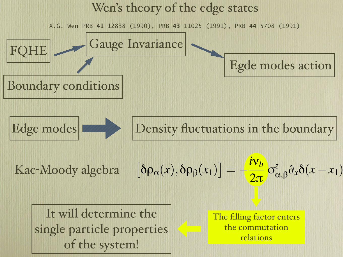
Wen’s theory of the edge statesX.G. Wen PRB 41 12838 (1990), PRB 43 11025 (1991), PRB 44 5708 (1991)

Gauge Invariance

Boundary conditionsEgde modes action

FQHE

Edge modes Density fluctuations in the boundary

Kac-Moody algebra

The filling factor enters the commutation

relations

[!"#(x),!"$(x1)

]=−i%b

2&'z#,$(x!(x− x1)

It will determine the single particle properties

of the system!

Experiments on the Luttinger Liquid exponent M. Grayson, D.C. Tsui, L.N. Pfeiffer, K.W. West, and A.M. Chang PRL 80 1062 (1998)

The experiments clearly show that the Chiral Luttinger tunneling

exponent varies continuously with the filling factor

Tunneling from a 3D electron gas to an edge of the FQHE

I !V!

!=1

"b

Edge states as hydrodynamical modesR. D’Agosta, R. Raimondi and G. Vignale PRB 90 (2003)

The density fluctuations are located in the region where the equilibrium density has the large derivative

Lowest Landau Levelprojection q!! 1

Hydrodynamic approximation

HT =Z!"(r)V (r,r1)!"(r1) d!rd!r1

[!"(!r),!"(!r1)] =−i"2#i j$i"0(!r)$ j!(!r−!r1) i, j ∈ {x,y}

!t"#(!r, t) = "2!i#0(!r)$i jZV (r,r1)"#(!r1, t) d!r1

Edge states as hydrodynamical modes II

Our edge excitations follow the same algebra of an interacting chiral Luttinger Liquid but we have not assumed the presence

of a fully developed Quantum Hall phase

y

H =1

2

Z!"#(x)V#,$(x,x1)!"$(x1) dxdx1

[!"#(x),!"$(x1)

]=−i%b

2&'z#,$(x!(x− x1)

!"#(x) =Z#!"(x,y) dy

We integrate over the shaded region to define

the edge excitation !," ∈ {R,L}

Solution of the interacting Hamiltonian

Bosonization:

Eqn of motion: !"n(x) form an orthonormal and complete

base for the Hilbert space

• Define

• Boson propagator

• Electron creation operator

!"#(x) =√$b

2% &n>0

bn'n

#(x)+b†n'n#

∗(x)

Single Particle operators:

!"#(x) = $x%#(x, t)

D!,"(x,x1,#) = −2$iZ %

0

d#〈[&!(x, t),&"(x1,0)]〉ei#t!†"(x) =U"e

−ie∗e

2#$b%"(x)

Calculation of the conductance

II

#4#1

#2 #3

#5#6

!Ii ="j

Gi j(V )!Vj

!j

Gi j =!i

Gi j = 0

Definition

Sum rules

The conductances can be related to the boson propagator

Gi j =−ie2

h̄!",#

$",i$#, j lim%→0

D(xi,x j,%)

V!,"(x,x1) = #(x− x1)V!," Gi j =!be

2

h"(xi− xi+1)

The Constriction

We model the constriction by assuming

VR,R(x,x1) =VL,L(x,x1) =V1

VR,L(x,x1) ={V2 |x| > a

V1

2|x| < a

V2

V2

V1

2

R

L

a

We solve the eqn of motion with scattering boundary conditions and calculate the transmission and reflection coefficients

The presence of the constriction does not modify the response function at zero bias: we recover the exact quantization of the

conductance

Phenomenological theory of the tunneling

HT = ! "†R(0)"L(0)+ !∗ "†

L(0)"R(0)

! - is assumed to be a phenomenological constant with no dependence on temperature or energy scale

(we will reanalyze this assumption later!)- is due to the non complete localization of the states in the

right or left edge

In linear response theory:

Rxx ! "#Im

Z $

0

ei#tImG

−(t,0)dt

G−(t,x) = 〈!†

L(t,x)!R(t,x)!†

R(0,0)!L(0,0)〉

Results for the tunneling between two edges If we remove the constriction we recover the Wen’s result

X.G. Wen PRB 43 11025 (1991), C.L. Kane and M.P.A Fisher PRB 51 13449 (1995)

The presence of the constriction introduces two different behaviors (i.e. two characteristic exponents) in the time

domain. The separation is given by the time an edge wave needs to travel trough the constriction.

R. D’Agosta et al. PRB 90 (2003)

Rxx(T,0) ! T2"b−2, Rxx(0,V ) !V 2"b−2

The presence of the interaction renormalizes the exponent

!b→ !be−2" (tanh(2") =V

1

2/V1)

Some experimental resultRecently the tunneling between two edges of the same

FQHE has been experimentally studied S. Roddaro et al. PRL 90 046805 (2003)

-3 -2 -1 0 1 2 3

V [mV]

2

3

4

5

6

7

dI T

/dV

T [µ

S]

T=30 mkT=100 mKT=200 mKT=300 mKT=400 mK

T=500 mKT=700 mKT=900 mK

B=6 T

At high temperature the peak seems agree with the theories

At low temperature the deep is not expected! (Strong coupling)

To address this experimental result we focus on the tunneling

amplitude!

!b = 1/3

G=dIT

dVT

Tunneling amplitude

The tunneling can be due to the incomplete

localization of the wave function in the edges

Being proportional to the superposition of wave functions belonging to different edges it is usually small and the

tunneling is usually treated as a perturbation

! " 〈#R|#L〉

The tunneling can be mediated by the presence of impurities that break down the translational

invariance

Tunneling amplitude

G

ϕL ϕR

D

dG

All the electrons occupy the Lowest Landau level

! "

Z#R(!x)#∗L(!x) d!x " e

− d2

4"2

A small variation of the edge distance affects significantly

the tunneling amplitude!

!

d/2}}

"

x

"="bV(x)

F [n] = E[n]−TS[n]In the incompressible region

!(x)≡ !b

Edge position: a simple model

n(x) =!(x)2"!2

S=− kB

2!!2

Z"(x) ln"(x)+ [1−"(x)] ln[1−"(x)] dx

!

!n(x)F [n] =U"(x)+V (x)+ kBT ln

["(x)

1−"(x)]

= µ

In the compressible region

E[n] =U

4!!2

Zn(x)2 dx+

ZV (x)n(x) dx

Edge position: a simple model II

The edge position is determined by

!(x0) = !b

d(T ) = d(0)+2x0(T )

In the simplest case V (x) = eEx

x0(T ) =kBT

U

ln(1−!b)!2b

"

µ(T ) = µ(0)+kbT

!b[!b ln!b+(1−!b) ln(1−!b)]

Particle number conservation N =Z !

x0

n(x) dx

Edge position: a simple approachAt zero temperature the edge position is determined by the

minimization of the electrostatic energyD.B. Chklovskii et al. PRB 46 4026 (1992), PRB 47 12605 (1993)

T != 0 minimize the free energy

F(d+!d) = F(d)+1

2"2dE(d)(!d)2−T"dS(d)!d

!d " T

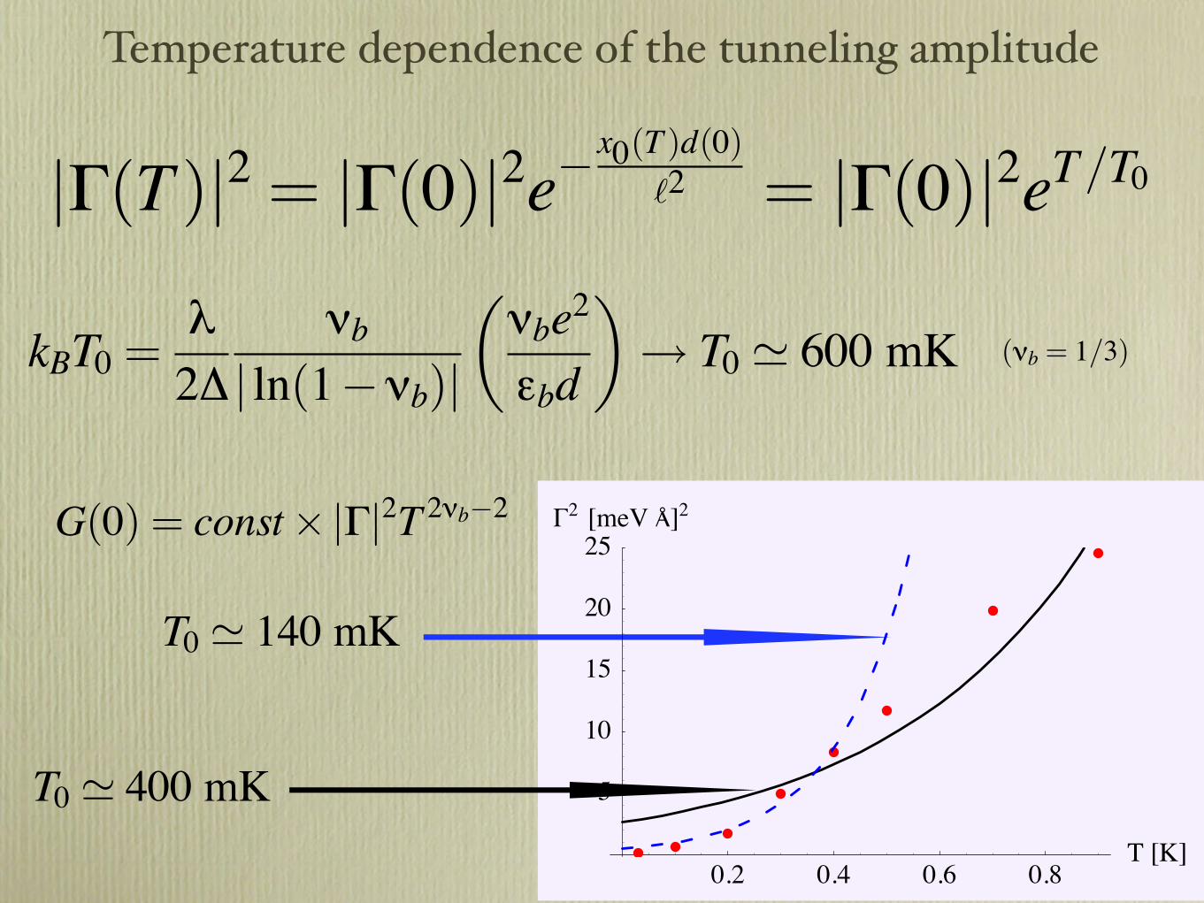
Temperature dependence of the tunneling amplitude

|!(T )|2 = |!(0)|2e−x0(T )d(0)!2 = |!(0)|2eT/T0

T0 ! 140 mK

T0 ! 400 mK0.2 0.4 0.6 0.8

T !K"

5

10

15

20

25

!2 !meV !"2G(0) = const× |!|2T 2"b−2

(!b = 1/3)kBT0 =!

2"

#b

| ln(1−#b)|(#be

2

$bd

)→ T0 # 600 mK

Recent experimentsS. Roddaro et al. cond/mat 043318 (2004)

kBT0 =!

2"

#b

| ln(1−#b)|(#be

2

$bd

)

-600 -400 -200 0 200 400 600 800

0

20

40

60

80

-80 0 80

5

10

15

20

25

!" = 2/7

!" = 1/4

!" = 1/5

! = 1

dV

/dI(

k#

)

V(µV)

! = 1/3T = 50 mK

-0.18 V-0.20 V

-0.26 V-0.32 V

-0.40 V

-0.50 V

dV

/dI(

k#

)

VT(µV)

Vg = -0.60 V

Extensions

• A better treatment of the electrostatic energy or a better approximation for the confining potential can improve the estimate for the temperature scale but we expect that it cannot modify the general scenario we have presented here

• The presence of different chemical potentials in the edges implies a rigid shift of the edge positions thus leaving their distance untouched

• For very small temperature the prediction of the RG is recovered because the tunneling amplitude goes to a constant

Conclusions

• The chiral luttinger liquid model can be used to study the phenomenology of the edge states of the FQHE

• We have extended the previous theory in order to consider the possibility of continuous variation of the filling factor

• We have then considered the dependence of the tunneling amplitude on geometrical factors and thus on temperature. Our results are in qualitative agreement with the available experimental data.

Acknowledgments

S. RoddaroV. PellegriniF. Beltram } Experiments in Pisa

NEST-INFM PRA-MesodyfNSF DMR-0313681 } Financial Support

Roberto Raimondi (Universita’ di Roma Tre)

Giovanni Vignale (University of Missouri) } Collaboration