Page 1
Copyright ⓒ The Korean Society for Aeronautical & Space SciencesReceived: May 12, 2017 Revised: September 7, 2017 Accepted: September 18, 2017
485 http://ijass.org pISSN: 2093-274x eISSN: 2093-2480
PaperInt’l J. of Aeronautical & Space Sci. 18(3), 485–497 (2017)DOI: http://dx.doi.org/10.5139/IJASS.2017.18.3.485
Structural Dynamic Analysis of a Space Launch Vehicle using an Axisymmetric Two-dimensional Shell Element
JiSoo Sim*Korea Aerospace Industries, LTD., 78, Gongdan 1-ro, Sanam-myeon, Sacheon, Gyeongsangnam-do 52529, Republic of Korea
SangGu Lee** Department of Mechanical and Aerospace Engineering, Seoul National University, Seoul 08826, Republic of Korea
JunBeom Kim***Republic of Korea Air Force, 221, Gonghang-ro, Dong-gu, Daegu 41052, Republic of Korea
SangJoon Shin****Department of Mechanical and Aerospace Engineering, Seoul National University, Seoul 08826, Republic of Korea
SeungSoo Park***** and WonSuk Ohm******Department of Mechanical Engineering, Yonsei University, 50, Yonsei-ro, Seodaemun-gu, Seoul 03772, Republic of Korea
Abstract
The pogo phenomenon refers to a type of multidiscipline-related instability found in space launch vehicles. It is caused
by coupling between the fuselage structure and other structural propulsion components. To predict the pogo phenomenon,
it is essential to undertake adequate structural modeling and to understand the characteristics of the feedlines and the
propulsion system. To do this, a modal analysis is conducted using axisymmetric two-dimensional shell elements. The analysis
is validated using examples of existing launch vehicles. Other applications and further plans for pogo analyses are suggested.
In addition, research on the pogo phenomenon of Saturn V and the space shuttle is conducted in order to constitute a pogo
stability analysis using the results of the present modal analysis.
Key words: Pogo phenomenon, Structural dynamic analysis, Two-dimensional axisymmetric shell, Rayleigh-ritz method
1. Introduction
Space launch vehicles exhibit many types of multidiscipline-
related instabilities caused by coupling between the fuselage
structure and other structural subsystem components [1].
These problems are mostly due to coupling between the
flight mechanics and flexural modes of a launch vehicle. The
buffet phenomenon involves the structural dynamics and the
aerodynamics. Longitudinal instability is related to coupling
between the structure and propulsion system. The term ‘pogo’
has been used in relation to this type of longitudinal instability
because its resulting motion resembles that of a pogo stick.
This paper primarily investigates the pogo phenomenon of
a launch vehicle, which is self-excited longitudinal dynamic
instability arising from the interaction between the launch
vehicle structure and the propulsion system. It is also one of
the most complex problems associated with liquid-propellant
launch vehicles. In order to predict the pogo phenomenon
This is an Open Access article distributed under the terms of the Creative Com-mons Attribution Non-Commercial License (http://creativecommons.org/licenses/by-nc/3.0/) which permits unrestricted non-commercial use, distribution, and reproduc-tion in any medium, provided the original work is properly cited.
* Researcher, Korea Aerospace Industries ** M.S student *** Researcher, Republic of Korea Air Force **** Professor, Corresponding author: [email protected] ***** M.S student ****** Professor
Page 2
DOI: http://dx.doi.org/10.5139/IJASS.2017.18.3.485 486
Int’l J. of Aeronautical & Space Sci. 18(3), 485–497 (2017)
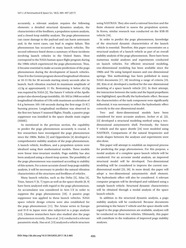
accurately, a relevant analysis requires the following
elements: a detailed structural dynamics analysis, the
characteristics of the feedlines, a propulsion system analysis,
and a closed-loop stability analysis. The pogo phenomenon
can cause damage to the payload and can harm astronauts
and, in the worst cases, can lead to engine failure. This
phenomenon has occurred in many launch vehicles. The
second reference listed shows a summary of these incidents
involving launch vehicles in the United States. Most
correspond to the NASA human space flight program during
the 1960s which experienced the pogo phenomenon. Thus,
it became essential to make accurate predictions of the pogo
phenomenon during the development of launch vehicles.
Titan II in the Gemini program showed longitudinal vibration
at 10-13 Hz for 30 seconds starting ninety seconds after its
launch. Such vibration reached its maximum amplitude of
±2.5g at approximately 11 Hz. Restraining it below ±0.25g
was required by NASA [2]. The Saturn V vehicle of the Apollo
project also showed pogo instability. AS-502 in 1968 recorded
longitudinal vibration of 5 Hz with maximum acceleration of
0.6 g between 105-140 seconds during the first-stage (S-IC)
burning process. Longitudinal oscillation was observed in
the first two Saturn V manned flights. Finally, a passive pogo
suppressor was installed in the space shuttle main engine
(SSME).
As mentioned in the previous section, the capability
to predict the pogo phenomenon accurately is crucial. A
few researchers have investigated the pogo phenomenon
since the 1960s. Rubin [3] and Oppenheim [4] developed a
comprehensive stability analysis of the pogo phenomenon.
A launch vehicle, feedlines, and a propulsion system were
idealized using their mathematical models. These models
were linear time-invariant models. Pogo stability has also
been analyzed using a closed-loop system. The possibility of
the pogo phenomenon was examined according to stability
of this system. For a more accurate closed-loop pogo stability
analysis, it will be necessary to predict the natural vibration
characteristics of the structures and feedlines of vehicles.
Many launch vehicles, such as the Delta [5], Atlas [4],
Titan, Saturn V [6, 7] types as well as the space shuttle [8, 9]
have been analyzed with regard to the pogo phenomenon.
An accumulator was considered in Ares I-X in order to
suppress the pogo phenomenon [10]. A passive pogo
suppressor was applied to these launch vehicles. NASA
space vehicle design criteria were also established for
the pogo phenomenon [11]. The Ariane series in Europe
and H-II in Japan were also subjected to a pogo analysis
[13]. Chinese researchers have also studied also the pogo
phenomenon recently. Zhao et al. [14] conducted a relevant
parametric study. Hao at el. [15] analyzed a vehicle structure
using NASTRAN. They also used a rational function and the
finite element method to assess the propulsion system.
In Korea, similar research was conducted on the KSR-III
vehicle [16].
In order to predict the pogo phenomenon, knowledge
of the structural dynamic characteristics of the launch
vehicle is essential. Therefore, this paper concentrates on a
structural analysis of a launch vehicle as part of an overall
stability analysis of the pogo phenomenon. There have been
numerous modal analyses and experiments conducted
on launch vehicles. For efficient structural modeling,
one-dimensional modeling has been available since the
1960s and 70s using lumped masses and one-dimensional
springs. This methodology has been published in many
NASA documents [17, 18] involving a range of criteria [19,
20]. Kim et al. developed a method for the one-dimensional
modeling of a space launch vehicle [21]. In their attempt,
the interaction between the tanks and the liquid propellants
was highlighted, specifically the hydroelastic effect. Because
the characteristics of the tank component were significantly
influential, it was necessary to reflect the hydroelastic effect
correctly in the one-dimensional model.
Two- and three-dimensional models have been
considered for more accurate analyses. Archer et al. [22,
23] developed a structural modeling method using a two-
dimensional axisymmetric shell. Previously, the Saturn
V vehicle and the space shuttle [24] were modeled using
NASTRAN. Comparisons of the natural frequencies and
mode shapes between the analyses and experiments were
also done.
This paper will attempt to establish an improved process
for predicting the pogo phenomenon. For this purpose, a
modal analysis of a complete space launch vehicle will be
conducted. For an accurate modal analysis, an improved
structural model will be developed. Two-dimensional
modeling will be considered to improve the current one-
dimensional model [25, 26]. In more detail, the paper will
adopt a two-dimensional axisymmetric shell element.
The hydroelastic effect will also be considered. A relevant
computer program will be developed and validated using a
sample launch vehicle. Structural dynamic characteristics
will be obtained through a modal analysis of the space
launch vehicle.
In addition to the structural dynamic analysis, a pogo
stability analysis will be conducted. Because documents
pertaining to the Saturn V vehicle and the space shuttle with
regard to the pogo phenomenon are available, analyses will
be conducted on those two vehicles. Ultimately, this paper
will contribute to the realization of improved pogo stability
analyses.
Page 3
487
JiSoo Sim Structural Dynamic Analysis of a Space Launch Vehicle using an Axisymmetric Two-dimensional Shell Element
http://ijass.org
2. Pogo Stability Analysis
2.1 Simplified Pogo Analysis of Saturn V
Pogo phenomenon analyses were developed and
conducted on the Saturn V vehicle and the space shuttle.
Fundamentally, the pogo phenomenon is analyzed using
two transfer functions in a closed-loop system. The first of
these is related to the structural system, G(s), and the second
is linked to the propulsion system, H(s), as shown in Fig. 1.
Therefore, G(s) and H(s) should reflect the characteristics of
a realistic system accurately. Such a closed system will be
analyzed under a certain flight condition in which the pogo
phenomenon could arise. Finally, the pogo phenomenon
will be predicted according to the stability of the closed-loop
system.
A pogo stability investigation of the Saturn V vehicle was
conducted by Sterett et al. [6]. They provided a complete
summary of the evolution of the pogo analysis methodology.
They analyzed the second stage, S-II, and the third stage,
S-IVB, as well as the first stage, S-IC. In addition, von
Pragenau [7] suggested a simplified pogo closed-loop
analysis, as shown in Fig. 2. This diagram illustrates a system
consisting of both a LOX tank and a thrust chamber among
several supply/propulsion components in a launch vehicle.
In his result, the relationships among the propellant force Ps,
the constant gain E, the thrust T, the force Fs, the cavitation
stiffness Ks, the orifice effect of the pump Ds, and the
disturbance force f were obtained. The thrust T was caused
by the propellant force Ps, and the force Fs was defined as
the sum of the thrust and the disturbance force f. These are
expressed in Eqs. (1) and (2).
sP E T⋅ = (1)
s sF P E f= ⋅ + (2)
In the structural model including the orifice effect, cavitation, and propellant, the propellant force
Ps was related to the force Fs. The relevant expression among the system, the propellant force, is
given in Eq. (3). All of these equations utilize the Laplace transform.
21
ss
s s s
FP
m m ms sm D K
=+ + +
(3)
The closed-loop system equation will become complete by combining Eqs. (2) and (3). The
resulting equation can then be written as follows:
21
s
s s s
fPm m mE s sm D K
=+ − + +
(4)
Finally, the stability will be determined by the sign of the eigenvalues s. Such a determination
criterion is expressed in Eq. (5).
1s
mEm
< + (5)
This complete relationship of the closed-loop system is illustrated by the block diagram shown in
Fig. 3. This result represents a simplified but complete process of analyzing the pogo phenomenon.
2.2 Pogo Suppression in the Space Shuttle
For the space shuttle, a relevant pogo integration panel was organized by various NASA research
centers and contractors [8]. As a result, a passive pogo suppressor was developed and installed,
although both passive and active devices were investigated simultaneously. The relevant analytical
model and the methodology used were quite systematic. Owing to the specific configuration of the
space shuttle, with an external tank, a feedline of a significant length (31 m) was designed and
adopted. Liquid oxygen is significantly heavier than liquid hydrogen, which is the main fuel of the
space shuttle. Therefore, the analytical model of the space shuttle was composed of a LOX tank, a
6
, (1)sP E T⋅ = (1)
s sF P E f= ⋅ + (2)
In the structural model including the orifice effect, cavitation, and propellant, the propellant force
Ps was related to the force Fs. The relevant expression among the system, the propellant force, is
given in Eq. (3). All of these equations utilize the Laplace transform.
21
ss
s s s
FP
m m ms sm D K
=+ + +
(3)
The closed-loop system equation will become complete by combining Eqs. (2) and (3). The
resulting equation can then be written as follows:
21
s
s s s
fPm m mE s sm D K
=+ − + +
(4)
Finally, the stability will be determined by the sign of the eigenvalues s. Such a determination
criterion is expressed in Eq. (5).
1s
mEm
< + (5)
This complete relationship of the closed-loop system is illustrated by the block diagram shown in
Fig. 3. This result represents a simplified but complete process of analyzing the pogo phenomenon.
2.2 Pogo Suppression in the Space Shuttle
For the space shuttle, a relevant pogo integration panel was organized by various NASA research
centers and contractors [8]. As a result, a passive pogo suppressor was developed and installed,
although both passive and active devices were investigated simultaneously. The relevant analytical
model and the methodology used were quite systematic. Owing to the specific configuration of the
space shuttle, with an external tank, a feedline of a significant length (31 m) was designed and
adopted. Liquid oxygen is significantly heavier than liquid hydrogen, which is the main fuel of the
space shuttle. Therefore, the analytical model of the space shuttle was composed of a LOX tank, a
6
. (2)
In the structural model including the orifice effect,
cavitation, and propellant, the propellant force Ps was
related to the force Fs. The relevant expression among the
system, the propellant force, is given in Eq. (3). All of these
equations utilize the Laplace transform.
sP E T⋅ = (1)
s sF P E f= ⋅ + (2)
In the structural model including the orifice effect, cavitation, and propellant, the propellant force
Ps was related to the force Fs. The relevant expression among the system, the propellant force, is
given in Eq. (3). All of these equations utilize the Laplace transform.
21
ss
s s s
FP
m m ms sm D K
=+ + +
(3)
The closed-loop system equation will become complete by combining Eqs. (2) and (3). The
resulting equation can then be written as follows:
21
s
s s s
fPm m mE s sm D K
=+ − + +
(4)
Finally, the stability will be determined by the sign of the eigenvalues s. Such a determination
criterion is expressed in Eq. (5).
1s
mEm
< + (5)
This complete relationship of the closed-loop system is illustrated by the block diagram shown in
Fig. 3. This result represents a simplified but complete process of analyzing the pogo phenomenon.
2.2 Pogo Suppression in the Space Shuttle
For the space shuttle, a relevant pogo integration panel was organized by various NASA research
centers and contractors [8]. As a result, a passive pogo suppressor was developed and installed,
although both passive and active devices were investigated simultaneously. The relevant analytical
model and the methodology used were quite systematic. Owing to the specific configuration of the
space shuttle, with an external tank, a feedline of a significant length (31 m) was designed and
adopted. Liquid oxygen is significantly heavier than liquid hydrogen, which is the main fuel of the
space shuttle. Therefore, the analytical model of the space shuttle was composed of a LOX tank, a
6
.
(3)
The closed-loop system equation will become complete
by combining Eqs. (2) and (3). The resulting equation can
then be written as follows:
sP E T⋅ = (1)
s sF P E f= ⋅ + (2)
In the structural model including the orifice effect, cavitation, and propellant, the propellant force
Ps was related to the force Fs. The relevant expression among the system, the propellant force, is
given in Eq. (3). All of these equations utilize the Laplace transform.
21
ss
s s s
FP
m m ms sm D K
=+ + +
(3)
The closed-loop system equation will become complete by combining Eqs. (2) and (3). The
resulting equation can then be written as follows:
21
s
s s s
fPm m mE s sm D K
=+ − + +
(4)
Finally, the stability will be determined by the sign of the eigenvalues s. Such a determination
criterion is expressed in Eq. (5).
1s
mEm
< + (5)
This complete relationship of the closed-loop system is illustrated by the block diagram shown in
Fig. 3. This result represents a simplified but complete process of analyzing the pogo phenomenon.
2.2 Pogo Suppression in the Space Shuttle
For the space shuttle, a relevant pogo integration panel was organized by various NASA research
centers and contractors [8]. As a result, a passive pogo suppressor was developed and installed,
although both passive and active devices were investigated simultaneously. The relevant analytical
model and the methodology used were quite systematic. Owing to the specific configuration of the
space shuttle, with an external tank, a feedline of a significant length (31 m) was designed and
adopted. Liquid oxygen is significantly heavier than liquid hydrogen, which is the main fuel of the
space shuttle. Therefore, the analytical model of the space shuttle was composed of a LOX tank, a
6
.
(4)
Finally, the stability will be determined by the sign of the
eigenvalues s. Such a determination criterion is expressed in
Eq. (5).
sP E T⋅ = (1)
s sF P E f= ⋅ + (2)
In the structural model including the orifice effect, cavitation, and propellant, the propellant force
Ps was related to the force Fs. The relevant expression among the system, the propellant force, is
given in Eq. (3). All of these equations utilize the Laplace transform.
21
ss
s s s
FP
m m ms sm D K
=+ + +
(3)
The closed-loop system equation will become complete by combining Eqs. (2) and (3). The
resulting equation can then be written as follows:
21
s
s s s
fPm m mE s sm D K
=+ − + +
(4)
Finally, the stability will be determined by the sign of the eigenvalues s. Such a determination
criterion is expressed in Eq. (5).
1s
mEm
< + (5)
This complete relationship of the closed-loop system is illustrated by the block diagram shown in
Fig. 3. This result represents a simplified but complete process of analyzing the pogo phenomenon.
2.2 Pogo Suppression in the Space Shuttle
For the space shuttle, a relevant pogo integration panel was organized by various NASA research
centers and contractors [8]. As a result, a passive pogo suppressor was developed and installed,
although both passive and active devices were investigated simultaneously. The relevant analytical
model and the methodology used were quite systematic. Owing to the specific configuration of the
space shuttle, with an external tank, a feedline of a significant length (31 m) was designed and
adopted. Liquid oxygen is significantly heavier than liquid hydrogen, which is the main fuel of the
space shuttle. Therefore, the analytical model of the space shuttle was composed of a LOX tank, a
6
.(5)
This complete relationship of the closed-loop system is
illustrated by the block diagram shown in Fig. 3. This result
represents a simplified but complete process of analyzing
the pogo phenomenon.
2.2 Pogo Suppression in the Space Shuttle
For the space shuttle, a relevant pogo integration panel was
organized by various NASA research centers and contractors
[8]. As a result, a passive pogo suppressor was developed
and installed, although both passive and active devices
were investigated simultaneously. The relevant analytical
model and the methodology used were quite systematic.
Owing to the specific configuration of the space shuttle,
with an external tank, a feedline of a significant length (31
m) was designed and adopted. Liquid oxygen is significantly
heavier than liquid hydrogen, which is the main fuel of the
Fig. 1. Closed loop system of the pogo phenomenon
23
Fig. 1. Closed loop system of the pogo phenomenon
Fig. 2. Simplified pogo closed loop analysis
24
Fig. 2. Simplified pogo closed loop analysis
Page 4
DOI: http://dx.doi.org/10.5139/IJASS.2017.18.3.485 488
Int’l J. of Aeronautical & Space Sci. 18(3), 485–497 (2017)
space shuttle. Therefore, the analytical model of the space
shuttle was composed of a LOX tank, a longitudinal lateral
feedline, a low and high LOX pump, and a chamber [9], as
shown in Fig. 4. A few specific flight conditions, i.e., the lift
off, maximum dynamic pressure (max. Q), the condition
before solid rocket booster (SRB) jettison, and that after
SRB jettison, all prone to pogo instability, were selected
and analyzed. The analytical model used was composed
of 14 variables for the propulsion system. The variables
consisted of the generalized coordinates of the fuselage, qn,
the pressures of two thrust chamber points, P, and the flow
rates of the tank outlet to eight points, Q, as listed in Eq. (6).
In the generalized coordinates of the fuselage, qn, subscript n
denotes the n-th mode of the fuselage.
longitudinal lateral feedline, a low and high LOX pump, and a chamber [9], as shown in Fig. 4. A few
specific flight conditions, i.e., the lift off, maximum dynamic pressure (max. Q), the condition before
solid rocket booster (SRB) jettison, and that after SRB jettison, all prone to pogo instability, were
selected and analyzed. The analytical model used was composed of 14 variables for the propulsion
system. The variables consisted of the generalized coordinates of the fuselage, nq , the pressures of
two thrust chamber points, P, and the flow rates of the tank outlet to eight points, Q, as listed in Eq.
(6). In the generalized coordinates of the fuselage, nq , subscript n denotes the n-th mode of the
fuselage.
2 4 5 7 8 2 3 4 5 7 8ˆ { , , , , , , , , , , , , , }c t nH P P P P P P Q Q Q Q Q Q Q q= (6)
ˆ{[ ( )] [ ][ ( )]} 0V s E F s H+ ⋅ = (7)
The complete system became a 14-order variable system, as expressed by Eq. (7). [V(s)] is the
complete system, composed of both structural and propulsion state variables. [E] is the position of the
pogo suppressor. [F(s)] denotes the characteristics of the pogo suppressor. Pogo instability was
examined through an eigenvalue analysis of the system. This was done by employing several
structural modes of each flight condition and varying the natural frequencies by ±15%. Pogo
instability occurred when the damping ratio decreased significantly and became negative. This
analysis procedure suggested what would be required for formulating the pogo analysis. The first
variables needed would be the characteristics of the structural system in terms of the generalized
coordinates, here represented by q. The second would be an analytical model of the feedlines and
propulsion system in terms of the pressures and flow rates. The relationship between the structural
system q and the propulsion system P and Q would also be needed.
3. Structural Modeling and Modal Analysis
3.1 Modal Analysis of the Launch Vehicles
This section focuses on the structural dynamic response of a launch vehicle. The transfer function
G(s) will be required to predict the response. G(s) is referred to as “the plant” in Fig. 3. The transfer
function G(s) refers to the natural frequencies and mode shapes of the launch vehicle. A modal
7
, (6)
longitudinal lateral feedline, a low and high LOX pump, and a chamber [9], as shown in Fig. 4. A few
specific flight conditions, i.e., the lift off, maximum dynamic pressure (max. Q), the condition before
solid rocket booster (SRB) jettison, and that after SRB jettison, all prone to pogo instability, were
selected and analyzed. The analytical model used was composed of 14 variables for the propulsion
system. The variables consisted of the generalized coordinates of the fuselage, nq , the pressures of
two thrust chamber points, P, and the flow rates of the tank outlet to eight points, Q, as listed in Eq.
(6). In the generalized coordinates of the fuselage, nq , subscript n denotes the n-th mode of the
fuselage.
2 4 5 7 8 2 3 4 5 7 8ˆ { , , , , , , , , , , , , , }c t nH P P P P P P Q Q Q Q Q Q Q q= (6)
ˆ{[ ( )] [ ][ ( )]} 0V s E F s H+ ⋅ = (7)
The complete system became a 14-order variable system, as expressed by Eq. (7). [V(s)] is the
complete system, composed of both structural and propulsion state variables. [E] is the position of the
pogo suppressor. [F(s)] denotes the characteristics of the pogo suppressor. Pogo instability was
examined through an eigenvalue analysis of the system. This was done by employing several
structural modes of each flight condition and varying the natural frequencies by ±15%. Pogo
instability occurred when the damping ratio decreased significantly and became negative. This
analysis procedure suggested what would be required for formulating the pogo analysis. The first
variables needed would be the characteristics of the structural system in terms of the generalized
coordinates, here represented by q. The second would be an analytical model of the feedlines and
propulsion system in terms of the pressures and flow rates. The relationship between the structural
system q and the propulsion system P and Q would also be needed.
3. Structural Modeling and Modal Analysis
3.1 Modal Analysis of the Launch Vehicles
This section focuses on the structural dynamic response of a launch vehicle. The transfer function
G(s) will be required to predict the response. G(s) is referred to as “the plant” in Fig. 3. The transfer
function G(s) refers to the natural frequencies and mode shapes of the launch vehicle. A modal
7
. (7)
The complete system became a 14-order variable system,
as expressed by Eq. (7). [V(s)] is the complete system,
composed of both structural and propulsion state variables.
[E] is the position of the pogo suppressor. [F(s)] denotes the
characteristics of the pogo suppressor. Pogo instability was
examined through an eigenvalue analysis of the system.
This was done by employing several structural modes of
each flight condition and varying the natural frequencies
by ±15%. Pogo instability occurred when the damping
ratio decreased significantly and became negative. This
analysis procedure suggested what would be required for
formulating the pogo analysis. The first variables needed
would be the characteristics of the structural system in terms
of the generalized coordinates, here represented by q. The
second would be an analytical model of the feedlines and
propulsion system in terms of the pressures and flow rates.
The relationship between the structural system q and the
propulsion system P and Q would also be needed.
3. Structural Modeling and Modal Analysis
3.1 Modal Analysis of the Launch Vehicles
This section focuses on the structural dynamic response of
a launch vehicle. The transfer function G(s) will be required
to predict the response. G(s) is referred to as “the plant”
in Fig. 3. The transfer function G(s) refers to the natural
frequencies and mode shapes of the launch vehicle. A modal
analysis will be conducted to determine the transfer function
G(s) via an appropriate structural model. The modal analysis
proceeds as follows. Assuming that the launch vehicle is an
undamped system, mass and stiffness matrices are used in
the modal analysis. These are expressed by Eq. (8).
, (8)
, (9)
. (10)
Equation (8) can be rearranged to become Eq. (10).
Equation (10) is an eigenvalue problem. When the eigenvalue
problem is solved, the eigenvalues will become the natural
frequencies and the eigenvectors will become the mode
shapes. Equation (11) is a generalized form using the natural
frequencies and mode shapes ϕ. Then, by dividing the left-
Fig. 3. Block diagram of a simplified pogo analysis
25
Fig. 3. Block diagram of a simplified pogo analysis
Fig. 4. Pogo analysis of the example space shuttle
26
Fig. 4. Pogo analysis of the example space shuttle
Page 5
489
JiSoo Sim Structural Dynamic Analysis of a Space Launch Vehicle using an Axisymmetric Two-dimensional Shell Element
http://ijass.org
hand side of Equation (11) by [M][ϕ], the second-order
differential equation for ξ can be simplified. This is expressed
as Equation (12). Equation (13) shows the situation when
the resultant force (excitation) exists. It is expressed in terms
of the generalized coordinates, and {ξ } denotes the modal
displacement.
, (11)
, (12)
. (13)
When Eqs. (12) and (13) are obtained, the transfer function
G(s) will be constructed.
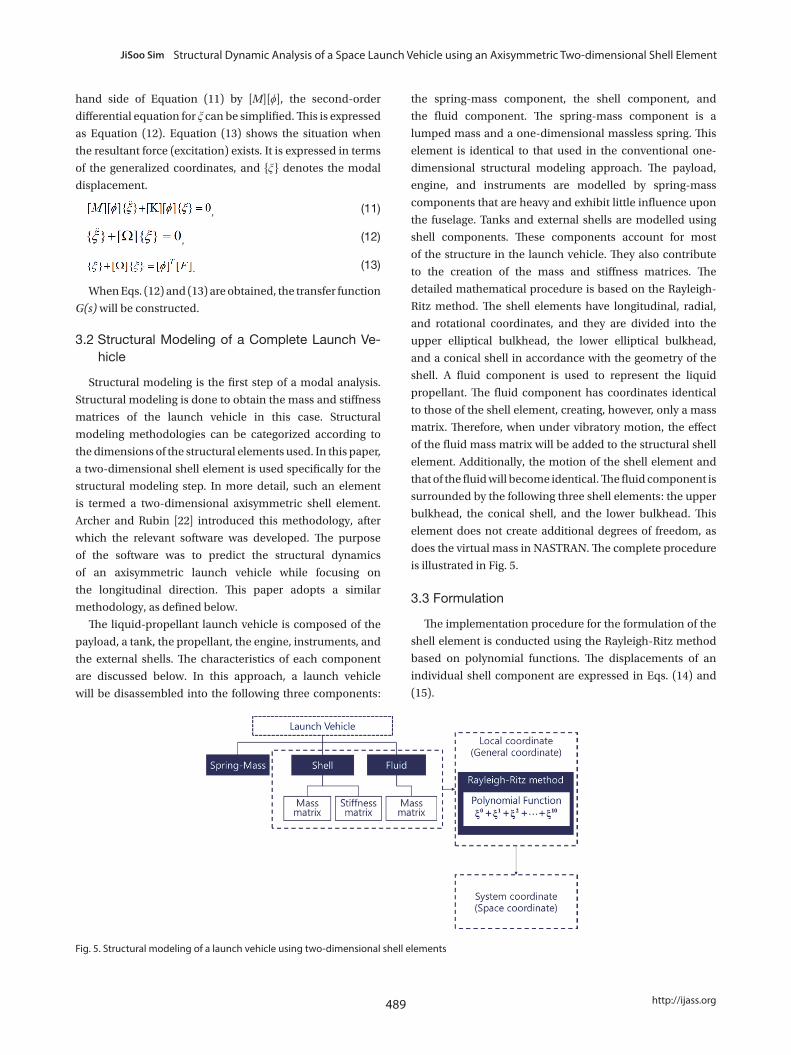
3.2 Structural Modeling of a Complete Launch Ve-hicle
Structural modeling is the first step of a modal analysis.
Structural modeling is done to obtain the mass and stiffness
matrices of the launch vehicle in this case. Structural
modeling methodologies can be categorized according to
the dimensions of the structural elements used. In this paper,
a two-dimensional shell element is used specifically for the
structural modeling step. In more detail, such an element
is termed a two-dimensional axisymmetric shell element.
Archer and Rubin [22] introduced this methodology, after
which the relevant software was developed. The purpose
of the software was to predict the structural dynamics
of an axisymmetric launch vehicle while focusing on
the longitudinal direction. This paper adopts a similar
methodology, as defined below.
The liquid-propellant launch vehicle is composed of the
payload, a tank, the propellant, the engine, instruments, and
the external shells. The characteristics of each component
are discussed below. In this approach, a launch vehicle
will be disassembled into the following three components:
the spring-mass component, the shell component, and
the fluid component. The spring-mass component is a
lumped mass and a one-dimensional massless spring. This
element is identical to that used in the conventional one-
dimensional structural modeling approach. The payload,
engine, and instruments are modelled by spring-mass
components that are heavy and exhibit little influence upon
the fuselage. Tanks and external shells are modelled using
shell components. These components account for most
of the structure in the launch vehicle. They also contribute
to the creation of the mass and stiffness matrices. The
detailed mathematical procedure is based on the Rayleigh-
Ritz method. The shell elements have longitudinal, radial,
and rotational coordinates, and they are divided into the
upper elliptical bulkhead, the lower elliptical bulkhead,
and a conical shell in accordance with the geometry of the
shell. A fluid component is used to represent the liquid
propellant. The fluid component has coordinates identical
to those of the shell element, creating, however, only a mass
matrix. Therefore, when under vibratory motion, the effect
of the fluid mass matrix will be added to the structural shell
element. Additionally, the motion of the shell element and
that of the fluid will become identical. The fluid component is
surrounded by the following three shell elements: the upper
bulkhead, the conical shell, and the lower bulkhead. This
element does not create additional degrees of freedom, as
does the virtual mass in NASTRAN. The complete procedure
is illustrated in Fig. 5.
3.3 Formulation
The implementation procedure for the formulation of the
shell element is conducted using the Rayleigh-Ritz method
based on polynomial functions. The displacements of an
individual shell component are expressed in Eqs. (14) and
(15).
..
..
Fig. 5. Structural modeling of a launch vehicle using two-dimensional shell elements
27
Fig. 5. Structural modeling of a launch vehicle using two-dimensional shell elements
Page 6
DOI: http://dx.doi.org/10.5139/IJASS.2017.18.3.485 490
Int’l J. of Aeronautical & Space Sci. 18(3), 485–497 (2017)
(14)
(15)
( )10
0
nk kn
n
u aξ ξ=
=∑ , ( )10
0
nl ln
n
v bξ ξ=
=∑ (16)
The displacements of the shell and the direction of the u(ξ) and v(ξ) coordinates are shown in Fig. 6.
Equation (16) is the formulation of a mode shape using the polynomial functions. kna and lnb are
arbitrarily specified coefficients, and ξ is a dimensionless variable corresponding to the geometry of
the shell. This variable can be described under the following three categories: the conical shell, the
upper bulkhead, and the lower bulkhead, as shown in Fig. 7. The upper and lower bulkheads are
ellipsoidal shell elements.
0s sinL
ξ φ= (17)
(18)
(19)
Equations (17), (18), and (19) are the dimensionless variables of the conical shell, upper bulkhead,
and lower bulkhead. The shell stiffness and mass matrices are shown in Eqs. (20) and (21),
respectively.
(20)
1
( ) ( )U
k kk
u uξ α ξ=
=∑
1
( ) ( )V
l ll
v vξ β ξ=
=∑
o
φξφ
=
o
π φξπ φ−
=−
2 2 2 2
1 1 1 1 1 1
2 2 2 2
1 12 2 2 2
1 1 1 1 1 1
2 2 2 2
1 1
[ ]
U V
U U U U U V
U V
V V U V V V
V V V V
V V V V
KV V V V
V V V V
α α α α α β α β
α α α α α β α β
β α β α β β β β
β α β α β β β β
∂ ∂ ∂ ∂⋅⋅ ⋅ ⋅ ⋅ ⋅
∂ ∂ ∂ ∂ ∂ ∂ ∂ ∂ ∂ ∂ ∂ ∂
⋅⋅ ⋅ ⋅ ⋅ ⋅∂ ∂ ∂ ∂ ∂ ∂ ∂ ∂= ∂ ∂ ∂ ∂ ⋅⋅ ⋅ ⋅ ⋅ ⋅∂ ∂ ∂ ∂ ∂ ∂ ∂ ∂ ∂ ∂ ∂ ∂ ⋅⋅ ⋅ ⋅ ⋅ ⋅∂ ∂ ∂ ∂ ∂ ∂ ∂ ∂
10
,(14) (14)
(15)
( )10
0
nk kn
n
u aξ ξ=
=∑ , ( )10
0
nl ln
n
v bξ ξ=
=∑ (16)
The displacements of the shell and the direction of the u(ξ) and v(ξ) coordinates are shown in Fig. 6.
Equation (16) is the formulation of a mode shape using the polynomial functions. kna and lnb are
arbitrarily specified coefficients, and ξ is a dimensionless variable corresponding to the geometry of
the shell. This variable can be described under the following three categories: the conical shell, the
upper bulkhead, and the lower bulkhead, as shown in Fig. 7. The upper and lower bulkheads are
ellipsoidal shell elements.
0s sinL
ξ φ= (17)
(18)
(19)
Equations (17), (18), and (19) are the dimensionless variables of the conical shell, upper bulkhead,
and lower bulkhead. The shell stiffness and mass matrices are shown in Eqs. (20) and (21),
respectively.
(20)
1
( ) ( )U
k kk
u uξ α ξ=
=∑
1
( ) ( )V
l ll
v vξ β ξ=
=∑
o
φξφ
=
o
π φξπ φ−
=−
2 2 2 2
1 1 1 1 1 1
2 2 2 2
1 12 2 2 2
1 1 1 1 1 1
2 2 2 2
1 1
[ ]
U V
U U U U U V
U V
V V U V V V
V V V V
V V V V
KV V V V
V V V V
α α α α α β α β
α α α α α β α β
β α β α β β β β
β α β α β β β β
∂ ∂ ∂ ∂⋅⋅ ⋅ ⋅ ⋅ ⋅
∂ ∂ ∂ ∂ ∂ ∂ ∂ ∂ ∂ ∂ ∂ ∂
⋅⋅ ⋅ ⋅ ⋅ ⋅∂ ∂ ∂ ∂ ∂ ∂ ∂ ∂= ∂ ∂ ∂ ∂ ⋅⋅ ⋅ ⋅ ⋅ ⋅∂ ∂ ∂ ∂ ∂ ∂ ∂ ∂ ∂ ∂ ∂ ∂ ⋅⋅ ⋅ ⋅ ⋅ ⋅∂ ∂ ∂ ∂ ∂ ∂ ∂ ∂
10
,(15)
(14)
(15)
( )10
0
nk kn
n
u aξ ξ=
=∑ , ( )10
0
nl ln
n
v bξ ξ=
=∑ (16)
The displacements of the shell and the direction of the u(ξ) and v(ξ) coordinates are shown in Fig. 6.
Equation (16) is the formulation of a mode shape using the polynomial functions. kna and lnb are
arbitrarily specified coefficients, and ξ is a dimensionless variable corresponding to the geometry of
the shell. This variable can be described under the following three categories: the conical shell, the
upper bulkhead, and the lower bulkhead, as shown in Fig. 7. The upper and lower bulkheads are
ellipsoidal shell elements.
0s sinL
ξ φ= (17)
(18)
(19)
Equations (17), (18), and (19) are the dimensionless variables of the conical shell, upper bulkhead,
and lower bulkhead. The shell stiffness and mass matrices are shown in Eqs. (20) and (21),
respectively.
(20)
1
( ) ( )U
k kk
u uξ α ξ=
=∑
1
( ) ( )V
l ll
v vξ β ξ=
=∑
o
φξφ
=
o
π φξπ φ−
=−
2 2 2 2
1 1 1 1 1 1
2 2 2 2
1 12 2 2 2
1 1 1 1 1 1
2 2 2 2
1 1
[ ]
U V
U U U U U V
U V
V V U V V V
V V V V
V V V V
KV V V V
V V V V
α α α α α β α β
α α α α α β α β
β α β α β β β β
β α β α β β β β
∂ ∂ ∂ ∂⋅⋅ ⋅ ⋅ ⋅ ⋅
∂ ∂ ∂ ∂ ∂ ∂ ∂ ∂ ∂ ∂ ∂ ∂
⋅⋅ ⋅ ⋅ ⋅ ⋅∂ ∂ ∂ ∂ ∂ ∂ ∂ ∂= ∂ ∂ ∂ ∂ ⋅⋅ ⋅ ⋅ ⋅ ⋅∂ ∂ ∂ ∂ ∂ ∂ ∂ ∂ ∂ ∂ ∂ ∂ ⋅⋅ ⋅ ⋅ ⋅ ⋅∂ ∂ ∂ ∂ ∂ ∂ ∂ ∂
10
.(16)
The displacements of the shell and the direction of the
u(ξ) and v(ξ) coordinates are shown in Fig. 6. Equation (16)
is the formulation of a mode shape using the polynomial
functions. akn and bln are arbitrarily specified coefficients,
and ξ is a dimensionless variable corresponding to the
geometry of the shell. This variable can be described under
the following three categories: the conical shell, the upper
bulkhead, and the lower bulkhead, as shown in Fig. 7. The
upper and lower bulkheads are ellipsoidal shell elements.
(14)
(15)
( )10
0
nk kn
n
u aξ ξ=
=∑ , ( )10
0
nl ln
n
v bξ ξ=
=∑ (16)
The displacements of the shell and the direction of the u(ξ) and v(ξ) coordinates are shown in Fig. 6.
Equation (16) is the formulation of a mode shape using the polynomial functions. kna and lnb are
arbitrarily specified coefficients, and ξ is a dimensionless variable corresponding to the geometry of
the shell. This variable can be described under the following three categories: the conical shell, the
upper bulkhead, and the lower bulkhead, as shown in Fig. 7. The upper and lower bulkheads are
ellipsoidal shell elements.
0s sinL
ξ φ= (17)
(18)
(19)
Equations (17), (18), and (19) are the dimensionless variables of the conical shell, upper bulkhead,
and lower bulkhead. The shell stiffness and mass matrices are shown in Eqs. (20) and (21),
respectively.
(20)
1
( ) ( )U
k kk
u uξ α ξ=
=∑
1
( ) ( )V
l ll
v vξ β ξ=
=∑
o
φξφ
=
o
π φξπ φ−
=−
2 2 2 2
1 1 1 1 1 1
2 2 2 2
1 12 2 2 2
1 1 1 1 1 1
2 2 2 2
1 1
[ ]
U V
U U U U U V
U V
V V U V V V
V V V V
V V V V
KV V V V
V V V V
α α α α α β α β
α α α α α β α β
β α β α β β β β
β α β α β β β β
∂ ∂ ∂ ∂⋅⋅ ⋅ ⋅ ⋅ ⋅
∂ ∂ ∂ ∂ ∂ ∂ ∂ ∂ ∂ ∂ ∂ ∂
⋅⋅ ⋅ ⋅ ⋅ ⋅∂ ∂ ∂ ∂ ∂ ∂ ∂ ∂= ∂ ∂ ∂ ∂ ⋅⋅ ⋅ ⋅ ⋅ ⋅∂ ∂ ∂ ∂ ∂ ∂ ∂ ∂ ∂ ∂ ∂ ∂ ⋅⋅ ⋅ ⋅ ⋅ ⋅∂ ∂ ∂ ∂ ∂ ∂ ∂ ∂
10
,(17)
(14)
(15)
( )10
0
nk kn
n
u aξ ξ=
=∑ , ( )10
0
nl ln
n
v bξ ξ=
=∑ (16)
The displacements of the shell and the direction of the u(ξ) and v(ξ) coordinates are shown in Fig. 6.
Equation (16) is the formulation of a mode shape using the polynomial functions. kna and lnb are
arbitrarily specified coefficients, and ξ is a dimensionless variable corresponding to the geometry of
the shell. This variable can be described under the following three categories: the conical shell, the
upper bulkhead, and the lower bulkhead, as shown in Fig. 7. The upper and lower bulkheads are
ellipsoidal shell elements.
0s sinL
ξ φ= (17)
(18)
(19)
Equations (17), (18), and (19) are the dimensionless variables of the conical shell, upper bulkhead,
and lower bulkhead. The shell stiffness and mass matrices are shown in Eqs. (20) and (21),
respectively.
(20)
1
( ) ( )U
k kk
u uξ α ξ=
=∑
1
( ) ( )V
l ll
v vξ β ξ=
=∑
o
φξφ
=
o
π φξπ φ−
=−
2 2 2 2
1 1 1 1 1 1
2 2 2 2
1 12 2 2 2
1 1 1 1 1 1
2 2 2 2
1 1
[ ]
U V
U U U U U V
U V
V V U V V V
V V V V
V V V V
KV V V V
V V V V
α α α α α β α β
α α α α α β α β
β α β α β β β β
β α β α β β β β
∂ ∂ ∂ ∂⋅⋅ ⋅ ⋅ ⋅ ⋅
∂ ∂ ∂ ∂ ∂ ∂ ∂ ∂ ∂ ∂ ∂ ∂
⋅⋅ ⋅ ⋅ ⋅ ⋅∂ ∂ ∂ ∂ ∂ ∂ ∂ ∂= ∂ ∂ ∂ ∂ ⋅⋅ ⋅ ⋅ ⋅ ⋅∂ ∂ ∂ ∂ ∂ ∂ ∂ ∂ ∂ ∂ ∂ ∂ ⋅⋅ ⋅ ⋅ ⋅ ⋅∂ ∂ ∂ ∂ ∂ ∂ ∂ ∂
10
,(18)
(14)
(15)
( )10
0
nk kn
n
u aξ ξ=
=∑ , ( )10
0
nl ln
n
v bξ ξ=
=∑ (16)
The displacements of the shell and the direction of the u(ξ) and v(ξ) coordinates are shown in Fig. 6.
Equation (16) is the formulation of a mode shape using the polynomial functions. kna and lnb are
arbitrarily specified coefficients, and ξ is a dimensionless variable corresponding to the geometry of
the shell. This variable can be described under the following three categories: the conical shell, the
upper bulkhead, and the lower bulkhead, as shown in Fig. 7. The upper and lower bulkheads are
ellipsoidal shell elements.
0s sinL
ξ φ= (17)
(18)
(19)
Equations (17), (18), and (19) are the dimensionless variables of the conical shell, upper bulkhead,
and lower bulkhead. The shell stiffness and mass matrices are shown in Eqs. (20) and (21),
respectively.
(20)
1
( ) ( )U
k kk
u uξ α ξ=
=∑
1
( ) ( )V
l ll
v vξ β ξ=
=∑
o
φξφ
=
o
π φξπ φ−
=−
2 2 2 2
1 1 1 1 1 1
2 2 2 2
1 12 2 2 2
1 1 1 1 1 1
2 2 2 2
1 1
[ ]
U V
U U U U U V
U V
V V U V V V
V V V V
V V V V
KV V V V
V V V V
α α α α α β α β
α α α α α β α β
β α β α β β β β
β α β α β β β β
∂ ∂ ∂ ∂⋅⋅ ⋅ ⋅ ⋅ ⋅
∂ ∂ ∂ ∂ ∂ ∂ ∂ ∂ ∂ ∂ ∂ ∂
⋅⋅ ⋅ ⋅ ⋅ ⋅∂ ∂ ∂ ∂ ∂ ∂ ∂ ∂= ∂ ∂ ∂ ∂ ⋅⋅ ⋅ ⋅ ⋅ ⋅∂ ∂ ∂ ∂ ∂ ∂ ∂ ∂ ∂ ∂ ∂ ∂ ⋅⋅ ⋅ ⋅ ⋅ ⋅∂ ∂ ∂ ∂ ∂ ∂ ∂ ∂
10
.(19)
Equations (17), (18), and (19) are the dimensionless
variables of the conical shell, upper bulkhead, and lower
bulkhead. The shell stiffness and mass matrices are shown in
Eqs. (20) and (21), respectively.
(14)
(15)
( )10
0
nk kn
n
u aξ ξ=
=∑ , ( )10
0
nl ln
n
v bξ ξ=
=∑ (16)
The displacements of the shell and the direction of the u(ξ) and v(ξ) coordinates are shown in Fig. 6.
Equation (16) is the formulation of a mode shape using the polynomial functions. kna and lnb are
arbitrarily specified coefficients, and ξ is a dimensionless variable corresponding to the geometry of
the shell. This variable can be described under the following three categories: the conical shell, the
upper bulkhead, and the lower bulkhead, as shown in Fig. 7. The upper and lower bulkheads are
ellipsoidal shell elements.
0s sinL
ξ φ= (17)
(18)
(19)
Equations (17), (18), and (19) are the dimensionless variables of the conical shell, upper bulkhead,
and lower bulkhead. The shell stiffness and mass matrices are shown in Eqs. (20) and (21),
respectively.
(20)
1
( ) ( )U
k kk
u uξ α ξ=
=∑
1
( ) ( )V
l ll
v vξ β ξ=
=∑
o
φξφ
=
o
π φξπ φ−
=−
2 2 2 2
1 1 1 1 1 1
2 2 2 2
1 12 2 2 2
1 1 1 1 1 1
2 2 2 2
1 1
[ ]
U V
U U U U U V
U V
V V U V V V
V V V V
V V V V
KV V V V
V V V V
α α α α α β α β
α α α α α β α β
β α β α β β β β
β α β α β β β β
∂ ∂ ∂ ∂⋅⋅ ⋅ ⋅ ⋅ ⋅
∂ ∂ ∂ ∂ ∂ ∂ ∂ ∂ ∂ ∂ ∂ ∂
⋅⋅ ⋅ ⋅ ⋅ ⋅∂ ∂ ∂ ∂ ∂ ∂ ∂ ∂= ∂ ∂ ∂ ∂ ⋅⋅ ⋅ ⋅ ⋅ ⋅∂ ∂ ∂ ∂ ∂ ∂ ∂ ∂ ∂ ∂ ∂ ∂ ⋅⋅ ⋅ ⋅ ⋅ ⋅∂ ∂ ∂ ∂ ∂ ∂ ∂ ∂
10
,
(20)
(21)
V and T are the potential and kinetic energy, respectively. The coordinate used in the modeling of
the shell component is shown in Fig. 6.
( )21 22
o
s
V r N N M K M K N dsφ φ θ θ φ φ φ φ φπ ε ε r= + + + +∫ (22)
(23)
Each elemental stiffness matrix is formulated in Eq. (23); the potential energy is given by Eq. (22).
On the right-hand side of Eq. (22), ,φ θε ε denotes the strain, K ,Kφ θ represents the curvature, and
r is the meridional rotation. Finally, oNφ is the initial meridional stress. In an orthotropic shell,
N ,N ,M ,Mφ θ φ θ all refer to the stress in the meridional directions and principal directions in the hoop
[22]. C11, C12, C22, C33, C34, and C44 are the orthotropic stress-strain and orthotropic moment-curvature
coefficients. Finally, the elemental stiffness and mass matrices are obtained by Eqs. (24) and (25),
respectively. K1, K2, …, and K13 are the approximate analytical coefficients.
2 2 2 2
1 1 1 1 1 1
2 2 2 2
1 12 2 2 2
1 1 1 1 1 1
2 2 2 2
1 1
[M]
U V
U U U U U V
U V
V V U V V V
T T V V
T T V V
V V T T
V V T T
α α α α α β α β
α α α α α β α β
β α β α β β β β
β α β α β β β β
∂ ∂ ∂ ∂⋅⋅ ⋅ ⋅ ⋅ ⋅
∂ ∂ ∂ ∂ ∂ ∂ ∂ ∂ ∂ ∂ ∂ ∂
⋅⋅ ⋅ ⋅ ⋅ ⋅∂ ∂ ∂ ∂ ∂ ∂ ∂ ∂= ∂ ∂ ∂ ∂ ⋅⋅ ⋅ ⋅ ⋅ ⋅∂ ∂ ∂ ∂ ∂ ∂ ∂ ∂ ∂ ∂ ∂ ∂ ⋅⋅ ⋅ ⋅ ⋅ ⋅∂ ∂ ∂ ∂ ∂ ∂ ∂ ∂
11
.
(21)
V and T are the potential and kinetic energy, respectively.
The coordinate used in the modeling of the shell component
is shown in Fig. 6.
(21)
V and T are the potential and kinetic energy, respectively. The coordinate used in the modeling of
the shell component is shown in Fig. 6.
( )21 22
o
s
V r N N M K M K N dsφ φ θ θ φ φ φ φ φπ ε ε r= + + + +∫ (22)
(23)
Each elemental stiffness matrix is formulated in Eq. (23); the potential energy is given by Eq. (22).
On the right-hand side of Eq. (22), ,φ θε ε denotes the strain, K ,Kφ θ represents the curvature, and
r is the meridional rotation. Finally, oNφ is the initial meridional stress. In an orthotropic shell,
N ,N ,M ,Mφ θ φ θ all refer to the stress in the meridional directions and principal directions in the hoop
[22]. C11, C12, C22, C33, C34, and C44 are the orthotropic stress-strain and orthotropic moment-curvature
coefficients. Finally, the elemental stiffness and mass matrices are obtained by Eqs. (24) and (25),
respectively. K1, K2, …, and K13 are the approximate analytical coefficients.
2 2 2 2
1 1 1 1 1 1
2 2 2 2
1 12 2 2 2
1 1 1 1 1 1
2 2 2 2
1 1
[M]
U V
U U U U U V
U V
V V U V V V
T T V V
T T V V
V V T T
V V T T
α α α α α β α β
α α α α α β α β
β α β α β β β β
β α β α β β β β
∂ ∂ ∂ ∂⋅⋅ ⋅ ⋅ ⋅ ⋅
∂ ∂ ∂ ∂ ∂ ∂ ∂ ∂ ∂ ∂ ∂ ∂
⋅⋅ ⋅ ⋅ ⋅ ⋅∂ ∂ ∂ ∂ ∂ ∂ ∂ ∂= ∂ ∂ ∂ ∂ ⋅⋅ ⋅ ⋅ ⋅ ⋅∂ ∂ ∂ ∂ ∂ ∂ ∂ ∂ ∂ ∂ ∂ ∂ ⋅⋅ ⋅ ⋅ ⋅ ⋅∂ ∂ ∂ ∂ ∂ ∂ ∂ ∂
11
,(22)
.
(23)
Fig. 6. Coordinates of the shell elements
28
Fig. 6. Coordinates of the shell elements
(a) Conical shell
(b) Ellipsoidal shell
Fig. 7. Geometry of the shell element
29
Fig. 7. Geometry of the shell element
Page 7
491
JiSoo Sim Structural Dynamic Analysis of a Space Launch Vehicle using an Axisymmetric Two-dimensional Shell Element
http://ijass.org
Each elemental stiffness matrix is formulated in Eq. (23);
the potential energy is given by Eq. (22). On the right-hand
side of Eq. (22), εϕ, εθ denotes the strain, Kϕ, Kθ represents
the curvature, and ρ is the meridional rotation. Finally, Nϕ0
is the initial meridional stress. In an orthotropic shell, Nϕ,
Nθ, Mϕ, Nθ all refer to the stress in the meridional directions
and principal directions in the hoop [22]. C11, C12, C22, C33,
C34, and C44 are the orthotropic stress-strain and orthotropic
moment-curvature coefficients. Finally, the elemental
stiffness and mass matrices are obtained by Eqs. (24) and
(25), respectively. K1, K2, …, and K13 are the approximate
analytical coefficients.
(24)
(25)
The fluid component provides only the mass matrix. The fluid motion is expressed as a function of
the generalized displacements of the shell components. The fluid motion and coordinates are shown in
Fig. 8. The mass matrix of the fluid component is determined by Eq. (26). The fluid is assumed to be
incompressible and inviscid. ˆ ( )mu x is equal to the change in volume below a given location x
divided by the corresponding tank cross-sectional area. The radial fluid motion varies linearly with the
spatial coordinate.
( )3 0
ˆ ˆ ˆ ˆ ˆ ˆ ˆ ˆ[ ] 2 { ( )} { ( )} { ( , )} { ( , )}H r T T
bH
M r u x u x v x r v x r dr dxπ γ−
= ⋅ + ⋅∫ ∫ (26)
Each component of the shell and fluid is estimated to provide the mass and stiffness matrices.
These matrices are described in the local coordinates (generalized coordinates) shown in Fig. 5. These
matrices can be transformed into the system coordinates (spatial coordinates). As a result, all of the
components are combined to provide one mass and one stiffness matrix.
4. Numerical Results and Discussion
4.1 Construction of the Present Analysis
The present analysis is developed using the methodology explained in the previous sections.
MATLAB is used for the baseline program. The variable ‘sym’ is used to represent the symbolic
variables for the normalized variable when it changes from 0 to 1. The function ‘int’ is used to express
the definite integral for the matrix element. The eigenvalue problem is solved by the function ‘eig’.
The present numerical integration is conducted using a variable size in steps for enhanced accuracy
instead of the 16-point Gaussian weighting methodology described in the literature (Ref. 22).
1 2
31
4
13
( {u} {u} {u} {u}
[{u} {u} {u} {u} ][ ] 2[{v} {v} {v} {v} ]
[{v} {u} {u} {v} ]
T T
T T
T T
T T
r K K
KK r r dK
K
π φ
⋅ ⋅ + ⋅ ⋅ + ⋅ ⋅ + ⋅ = + ⋅ ⋅ + ⋅ + ⋅⋅ ⋅ + ⋅ ⋅ + ⋅
∫∫
12
,
(24)
.(25)
The fluid component provides only the mass matrix. The
fluid motion is expressed as a function of the generalized
displacements of the shell components. The fluid motion
and coordinates are shown in Fig. 8. The mass matrix of
the fluid component is determined by Eq. (26). The fluid is
assumed to be incompressible and inviscid.
(24)
(25)
The fluid component provides only the mass matrix. The fluid motion is expressed as a function of
the generalized displacements of the shell components. The fluid motion and coordinates are shown in
Fig. 8. The mass matrix of the fluid component is determined by Eq. (26). The fluid is assumed to be
incompressible and inviscid. ˆ ( )mu x is equal to the change in volume below a given location x
divided by the corresponding tank cross-sectional area. The radial fluid motion varies linearly with the
spatial coordinate.
( )3 0
ˆ ˆ ˆ ˆ ˆ ˆ ˆ ˆ[ ] 2 { ( )} { ( )} { ( , )} { ( , )}H r T T
bH
M r u x u x v x r v x r dr dxπ γ−
= ⋅ + ⋅∫ ∫ (26)
Each component of the shell and fluid is estimated to provide the mass and stiffness matrices.
These matrices are described in the local coordinates (generalized coordinates) shown in Fig. 5. These
matrices can be transformed into the system coordinates (spatial coordinates). As a result, all of the
components are combined to provide one mass and one stiffness matrix.
4. Numerical Results and Discussion
4.1 Construction of the Present Analysis
The present analysis is developed using the methodology explained in the previous sections.
MATLAB is used for the baseline program. The variable ‘sym’ is used to represent the symbolic
variables for the normalized variable when it changes from 0 to 1. The function ‘int’ is used to express
the definite integral for the matrix element. The eigenvalue problem is solved by the function ‘eig’.
The present numerical integration is conducted using a variable size in steps for enhanced accuracy
instead of the 16-point Gaussian weighting methodology described in the literature (Ref. 22).
1 2
31
4
13
( {u} {u} {u} {u}
[{u} {u} {u} {u} ][ ] 2[{v} {v} {v} {v} ]
[{v} {u} {u} {v} ]
T T
T T
T T
T T
r K K
KK r r dK
K
π φ
⋅ ⋅ + ⋅ ⋅ + ⋅ ⋅ + ⋅ = + ⋅ ⋅ + ⋅ + ⋅⋅ ⋅ + ⋅ ⋅ + ⋅
∫∫
12
is equal
to the change in volume below a given location x divided by
the corresponding tank cross-sectional area. The radial fluid
motion varies linearly with the spatial coordinate.
(24)
(25)
The fluid component provides only the mass matrix. The fluid motion is expressed as a function of
the generalized displacements of the shell components. The fluid motion and coordinates are shown in
Fig. 8. The mass matrix of the fluid component is determined by Eq. (26). The fluid is assumed to be
incompressible and inviscid. ˆ ( )mu x is equal to the change in volume below a given location x
divided by the corresponding tank cross-sectional area. The radial fluid motion varies linearly with the
spatial coordinate.
( )3 0
ˆ ˆ ˆ ˆ ˆ ˆ ˆ ˆ[ ] 2 { ( )} { ( )} { ( , )} { ( , )}H r T T
bH
M r u x u x v x r v x r dr dxπ γ−
= ⋅ + ⋅∫ ∫ (26)
Each component of the shell and fluid is estimated to provide the mass and stiffness matrices.
These matrices are described in the local coordinates (generalized coordinates) shown in Fig. 5. These
matrices can be transformed into the system coordinates (spatial coordinates). As a result, all of the
components are combined to provide one mass and one stiffness matrix.
4. Numerical Results and Discussion
4.1 Construction of the Present Analysis
The present analysis is developed using the methodology explained in the previous sections.
MATLAB is used for the baseline program. The variable ‘sym’ is used to represent the symbolic
variables for the normalized variable when it changes from 0 to 1. The function ‘int’ is used to express
the definite integral for the matrix element. The eigenvalue problem is solved by the function ‘eig’.
The present numerical integration is conducted using a variable size in steps for enhanced accuracy
instead of the 16-point Gaussian weighting methodology described in the literature (Ref. 22).
1 2
31
4
13
( {u} {u} {u} {u}
[{u} {u} {u} {u} ][ ] 2[{v} {v} {v} {v} ]
[{v} {u} {u} {v} ]
T T
T T
T T
T T
r K K
KK r r dK
K
π φ
⋅ ⋅ + ⋅ ⋅ + ⋅ ⋅ + ⋅ = + ⋅ ⋅ + ⋅ + ⋅⋅ ⋅ + ⋅ ⋅ + ⋅
∫∫
12
,(26)
Each component of the shell and fluid is estimated to
provide the mass and stiffness matrices. These matrices are
described in the local coordinates (generalized coordinates)
shown in Fig. 5. These matrices can be transformed into the
system coordinates (spatial coordinates). As a result, all of
the components are combined to provide one mass and one
stiffness matrix.
4. Numerical Results and Discussion
4.1 Construction of the Present Analysis
The present analysis is developed using the methodology
explained in the previous sections. MATLAB is used for the
baseline program. The variable ‘sym’ is used to represent
the symbolic variables for the normalized variable when
it changes from 0 to 1. The function ‘int’ is used to express
the definite integral for the matrix element. The eigenvalue
problem is solved by the function ‘eig’. The present numerical
integration is conducted using a variable size in steps
for enhanced accuracy instead of the 16-point Gaussian
weighting methodology described in the literature (Ref. 22).
4.2 Validation using a Sample Launch Vehicle
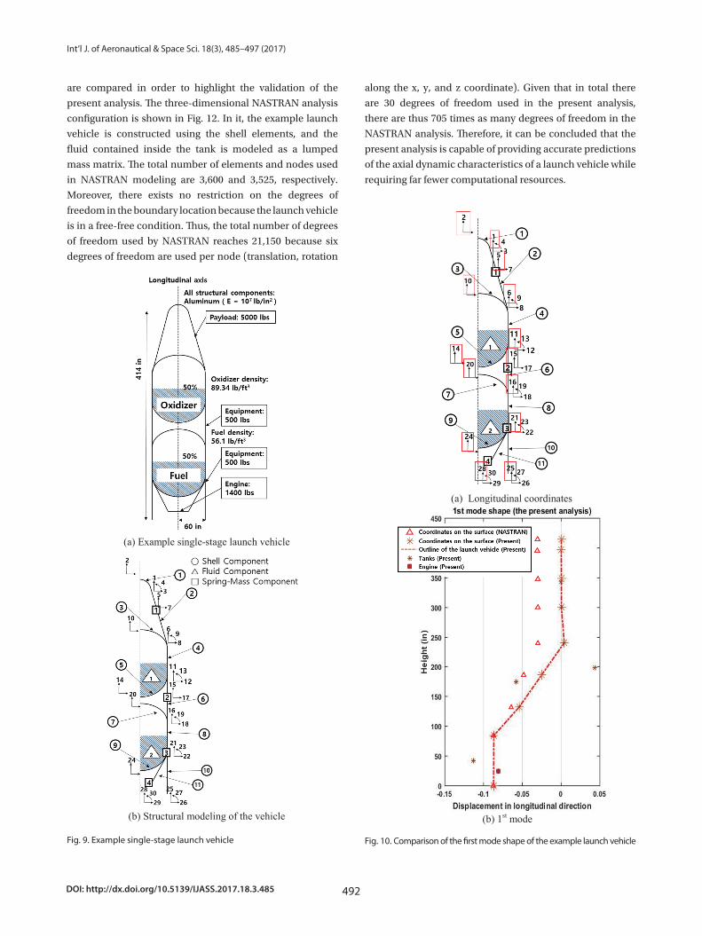
The example input and output were sourced from the
literature (Refs. 22 and 23). The present example is a single-
stage liquid launch vehicle that is axisymmetric, as shown in
Fig. 9 (a). A further structural model of the example is shown
in Fig. 9 (b). This model is composed of 11 shell components,
four spring-mass components, and two fluid components
and thus has a total of 30 degrees of freedom. The four
spring-mass elements are used to represent the payload,
equipment, and engine. The two fluid components serve to
represent the oxidizer and the fuel. The mass and stiffness
matrices are compared for each element against the existing
analytical prediction included in Ref. 22. The difference for
each element is less than 2%. Finally, mass and stiffness
matrices of 30 30 are obtained for the present example
launch vehicle. The eigenvalue problem is solved using these
matrices. The natural frequencies are then obtained by the
present program.
The results for the mode shape by the present analysis are
shown in Figs. 10(a) and 11. The relevant two-dimensional
model uses 30 coordinates. These coordinates are composed
of those in the longitudinal, radial, and rotational directions.
Among these, only the longitudinal direction coordinates
are used to show the relevant mode shapes. In Fig. 10(b), the
red line designates the mode shape of the complete launch
vehicle. The red star represents the coordinates of the tanks.
There are a few points outside of the line because bulkheads
exist inside a launch vehicle.
The three-dimensional NASTRAN eigenanalysis results Fig. 8. Definition of the fluid motion
30
Fig. 8. Definition of the fluid motion
Page 8
DOI: http://dx.doi.org/10.5139/IJASS.2017.18.3.485 492
Int’l J. of Aeronautical & Space Sci. 18(3), 485–497 (2017)
are compared in order to highlight the validation of the
present analysis. The three-dimensional NASTRAN analysis
configuration is shown in Fig. 12. In it, the example launch
vehicle is constructed using the shell elements, and the
fluid contained inside the tank is modeled as a lumped
mass matrix. The total number of elements and nodes used
in NASTRAN modeling are 3,600 and 3,525, respectively.
Moreover, there exists no restriction on the degrees of
freedom in the boundary location because the launch vehicle
is in a free-free condition. Thus, the total number of degrees
of freedom used by NASTRAN reaches 21,150 because six
degrees of freedom are used per node (translation, rotation
along the x, y, and z coordinate). Given that in total there
are 30 degrees of freedom used in the present analysis,
there are thus 705 times as many degrees of freedom in the
NASTRAN analysis. Therefore, it can be concluded that the
present analysis is capable of providing accurate predictions
of the axial dynamic characteristics of a launch vehicle while
requiring far fewer computational resources.
(a) Example single-stage launch vehicle
(b) Structural modeling of the vehicle
Fig. 9. Example single-stage launch vehicle
31
Fig. 9. Example single-stage launch vehicle
(a) Longitudinal coordinates
(b) 1st mode
Fig. 10. Comparison of the first mode shape of the example launch vehicle
32
Fig. 10. Comparison of the first mode shape of the example launch vehicle
Page 9
493
JiSoo Sim Structural Dynamic Analysis of a Space Launch Vehicle using an Axisymmetric Two-dimensional Shell Element
http://ijass.org
Table 1 shows the comparison results up to the ninth
axial mode. The discrepancy between the present and the
NASTRAN analysis result was found to as low as 0.7%. And,
relatively large differences are found for the first and third
modes. This is because both results have different number of
degrees of freedom per node. Three-dimensional NASTRAN
results describe the radial motions by using six degrees
of freedom in the longitudinal direction. On the contrary,
the present analysis expresses only an axial motion in the
longitudinal direction. Fig. 10 also shows the mode shapes
derived from the present analysis and NASTRAN. In Fig. 10
(b), the three-dimensional analysis results are illustrated
which correspond to the coordinates included in the surface
of the present analysis. A comparison of the two sets of results
shows that the results of the overall prediction are similar.
Fig. 11 shows additional mode shapes corresponding to the
second to the ninth mode as predicted by NASTRAN. And,
the first and third mode shapes are also in good agreement.
(a) 2nd mode (b) 3rd mode
(c) 4th mode (d) 5th mode
33 Fig. 11. Comparison of the 2nd~9th mode shapes of the example launch vehicle
Page 10
DOI: http://dx.doi.org/10.5139/IJASS.2017.18.3.485 494
Int’l J. of Aeronautical & Space Sci. 18(3), 485–497 (2017)
Therefore, both predictions give similar results regarding the
axial natural frequencies of the example launch vehicle.
It was also found that the pressure change caused by
the structural response at the bottom of the tanks will be
important for accurate predictions of the pogo phenomenon.
Such a change brings about variation of the pressures and
the flow rates of the feedlines. As a result, the thrust will
also change due to the pressure variation at the bottom of
the tank. For the example of the single-stage launch vehicle,
the fourteenth degree of freedom is assigned to the bottom
of the LOX tank. Therefore, changing the pressure can be
done after analyzing the response of the fourteenth degree
of freedom relative to the response of the complete launch
vehicle. This pressure change will finally be estimated using
the relationship between the structural acceleration and the
pressure disturbance.
(e) 6th mode (f) 7th mode
(g) 8th mode (h) 9th mode
Fig. 11. Comparison of the 2nd~9th mode shapes of the example launch vehicle
34
Fig. 11. Comparison of the 2nd~9th mode shapes of the example launch vehicle
Page 11
495
JiSoo Sim Structural Dynamic Analysis of a Space Launch Vehicle using an Axisymmetric Two-dimensional Shell Element
http://ijass.org
5. Conclusion
This paper suggests and develops an improved
methodology for the pogo phenomenon. Previous
researchers dealt with various launch vehicles in Europe
and Asia as well as some in the U.S. Accurate predictions are
required for the pogo phenomenon in a liquid-propellant
launch vehicle. This paper focused on the structural
modeling and on a modal analysis of a liquid-propellant
launch vehicle. Specifically, the transfer function G(s) was
estimated to develop the pogo analysis. The formulation and
analysis were developed using an approach which relied
on a two-dimensional axisymmetric shell element. The
present analysis was validated in comparison with three-
dimensional NASTRAN prediction results. The present
methodology using the axisymmetric shell element adopted
the Rayleigh-Ritz method. In this methodology, a liquid-
propellant launch vehicle was divided into the following
three components: the spring-mass, the shell, and the fluid
components. The present shell element differed from that
used in the general finite element method. Furthermore,
the fluid component did not generate additional degrees of
freedom. In more detail, the present numerical integration
was conducted using a variable step size instead of the
16-point Gaussian weighting methodology in order to
improve the accuracy.
Furthermore, the axial frequency predictions by the
present analysis were compared with the three–dimensional
NASTRAN analysis results. Both results yielded consistent
natural frequencies and mode shapes for the example
launch vehicle. The present analysis has an advantage in
terms of computational resource usage because it uses far
fewer degrees of freedom when compared with the three-
dimensional analysis.
In the future, several ideas will be added to the proposed
methodology in order to extract more accurate dynamic
characteristics of a launch vehicle. First, when the degrees
of freedom of the present shell element are expanded
to those for three dimensions, detailed launch vehicle
characteristics such as bending and breathing modes
will be available as well as the longitudinal modes. These
can be used to predict instability of the launch vehicle,
including the pogo phenomenon, more accurately. Second,
when the complex internal components of the launch
vehicle are modeled as simple shell elements based on
experimental results, a modal analysis can be conducted
without requiring a large number of degrees of freedom, as
required in as a three-dimensional full-scale finite element
computation. This will greatly improve the computational
efficiency of the analysis.
On the other hand, other launch vehicles can also be
analyzed using the methodology proposed here. Finally,
these results can be used to create a pogo analysis. The
chances of the natural frequencies overlapping with those
of the feedlines and the propulsion system can also be
estimated.
Fig. 12. NASTRAN three-dimensional analysis configuration
35
Fig. 12. NASTRAN three-dimensional analysis configuration
Table 1. Comparison of the natural frequencies between the present and three-dimensional NASTRAN analysisTable 1. Comparison of the natural frequencies between the present and three-dimensional NASTRAN analysis
Mode Natural frequencies by the present analysis (Hz)
Natural frequencies by 3-DNASTRAN analysis (Hz)
Difference between the present and NASTRAN (%)
1st mode 37.60 32.637 15.22nd 59.94 59.301 0.013rd 82.79 93.904 -11.84th 114.80 120.87 -5.025th 177.22 193.38 -8.356th 224.79 229.72 -2.147th 289.89 271.16 6.918th 376.16 382.24 -1.019th 450.34 459.26 -1.94
22
Page 12
DOI: http://dx.doi.org/10.5139/IJASS.2017.18.3.485 496
Int’l J. of Aeronautical & Space Sci. 18(3), 485–497 (2017)
Acknowledgement
This work was supported by the Advanced Research Center
Program (NRF-2013R1A5A1073861) through a grant from
the National Research Foundation of Korea (NRF) funded
by the Korean government (MSIP) through a contract with
the Advanced Space Propulsion Research Center at Seoul
National University.
Nomenclature
Ps = Propellant force
E = Thrust gain
f = Disturbance force
Ks = Cavitation stiffness of a pump inlet
Ds = Orifice effect of a pump
ms = Lox mass
m = Structure mass
[M] = Mass matrix
[K] = Stiffness matrix
ωn = Natural frequency
[ϕ] = Mode shape vector
u[ξ] = Displacement of the shell component in the
longitudinal direction
v[ξ] = Displacement of the shell component in the
radial direction
ξ = Dimensionless variable for the shell element
C11, C12, C22 = Orthotropic stress-strain coefficients
C33, C34, C44 = Orthotropic moment-curvature coefficients
t = Thickness of the shell
γa = Density of the shell
γb = Density of the fluid
x = Coordinate in the longitudinal direction
r = Coordinate in the radial direction
References
[1] Ryan, S. G., “Vibration Challenges in the Design of
NASA's Ares Launch Vehicles”, 2009 International Design
Engineering Technical Conference: 22nd Biennial Conference
on Mechanical Vibration and Noise, San Diego, CA, Aug. 30
- Sep. 2, 2009.
[2] Larsen, C. E., “NASA Experience with Pogo in Human
Spaceflight Vehicles”, NATO RTO Symposium ATV-152 on
Limit-Cycle Oscillations and Other Amplitude-Limited, Self-
Excited Vibrations, Norway, May 5-8, 2008.
[3] Rubin, S., “Longitudinal Instability of Liquid Rockets
Due to Propulsion Feedback (POGO)”, Journal of Spacecraft,
Vol. 3, No. 8, 1966, pp. 1188-1195.
[4] Oppenheim, B. W. and Rubin, S., “Advanced Pogo
Stability Analysis for Liquid Rockets”, Journal of Spacecraft
and Rockets, Vol. 30, No.3, 1993, pp. 360-373.
[5] Payne, J. G. and Rubin, S., “Pogo Suppression on the
Delta Vehicle”, AD-784833, 1974.
[6] Sterett, J. B. and Riley, G. F., “Saturn V/Apollo Vehicle Pogo
Stability Problems and Solutions”, AIAA 7th Annual Meeting
and Technological Display, Houston, TX, Oct. 19-22, 1970.
[7] von Pragenau, G. L., “Stability Analysis of Apollo-
Saturn V Propulsion and Structure Feedback Loop”, AIAA
Guidance, Control, and Flight Mechanics Conference, New
Jersey, NJ, Aug. 18-20, 1969.
[8] Doiron, H. H., “Space Shuttle Pogo Prevention”, Society
of Automotive Engineers Aerospace Meeting, Los Angeles, CA,
Nov. 14-17, 1977.
[9] Lock, M. H. and Rubin, S., “Passive Suppression of
Pogo on the Space Shuttle”, NASA CR-132452, 1974.
[10] Swanson, L. and Giel, T., “Design Analysis of the Ares
I Pogo Accumulator”, 45th AIAA/ASME/SAE/ASEE Joint
Propulsion Conference & Exhibit, Denver, CO, Aug. 2-5, 2009.
[11] Anonymous, “NASA Space Vehicle Design Criteria-
Prevention of Coupled Structure-Propulsion Instability
(POGO)”, NASA SP-8055, 1970.
[12] About, G., Bouveret, P. and Bonnal, C., “A New
Approach of Pogo Phenomenon Three-Dimensional Studies
on the Ariane 4 Launcher”, Acta Astronautica, Vol. 15, Issues
6–7, 1987, pp. 321-330.
[13] Ujino, T., Morino, Y., Kohsetsu, Y., Mori, T. and
Shirai, Y., “POGO Analysis on the H-II Launch Vehicle”, 30th
Structures, Structural Dynamics and Materials Conference,
Mobile, AL, April 3-5, 1989.
[14] Zhao, Z. and Ren, G., “Parameter Sturdy on Pogo
Stability of Liquid Rockets”, Journal of Spacecraft and Rockets,
Vol. 48, No. 3, 2011, pp. 537-541.
[15] Hao, Y., Tang, G. and Xu, D., “Finite-Element Modeling
and Frequency-Domain Analysis of Liquid-Propulsion
Launch Vehicle”, AIAA Journal, Vol. 53, No. 11, 2015.
[16] Chang, H. S., “A Study on the Analysis of Pogo and
its Suppression”, Master’s Thesis, Korea Advanced Institute
of Science and Technology, Department of Mechanical
Engineering, 2002.
[17] Pinson, L. D., “Longitudinal Spring Constants for
liquid-Propellant Tanks with Ellipsoidal Ends”, NASA TN
D-2220, 1964.
[18] Pengelley, C. D., “Natural Frequency of Longitudinal
Modes of Liquid Propellant Space Launch Vehicles”, Journal
of Spacecraft, Vol. 5, No. 12, 1968, pp. 1425-1431.
[19] Anonymous, “NASA Space Vehicle Design Criteria-
Natural Vibration Modal Analysis”, NASA SP-8012, 1970.
Page 13
497
JiSoo Sim Structural Dynamic Analysis of a Space Launch Vehicle using an Axisymmetric Two-dimensional Shell Element
http://ijass.org
[20] Anonymous, “NASA Space Vehicle Design Criteria-
Structural Vibration Prediction”, NASA SP-8050, 1970.
[21] Kim, J., Sim, J., Shin, S., Park, J. and Kim, Y., “Advanced
One-dimensional Dynamic Analysis Methodology for
Space Launch Vehicles Reflecting Liquid Components”,
Aeronautical Journal, in revision.
[22] Archer, J. S. and Rubin, C. P., “Improved Analytic
Longitudinal Response Analysis for Axisymmetric Launch
Vehicle”, Vol. 1, NASA CR-345, 1965.
[23] Rubin, C. P. and Wang, T. T., “Improved Analytic
Longitudinal Response Analysis for Axisymmetric Launch
Vehicle”, Vol. 2, NASA CR-346, 1965.
[24] Pinson, L. D. and Leadbetter, S. A., “Some Results
from 1/8-Scale Shuttle Model Vibration Studies”, Journal of
Spacecraft, Vol. 61, No. 1, 1979.
[25] Sim, J., Kim, J., Lee, S., Shin, S., Choi, H. and Yoon, W.,
“Further Extended Structural Modeling and Modal Analysis
of Liquid-Propellant Launch Vehicles for Pogo Analysis”,
AIAA SPACE Conference and Exposition, Long Beach, NJ,
Sep. 13-16, 2016.
[26] Sim, J., “Structural Dynamic Analysis of Space Launch
Vehicle Using Axisymmetric Shell Element Including
Hydroelastic Effect for Pogo Stability Analysis”, Master’s
Thesis, Seoul National University, 2017.