STRUCTURAL DYNAMIC MODIFICATION OF VIBRATING...

STRUCTURAL DYNAMIC MODIFICATION OF

VIBRATING STRUCTURES USING

TOPOLOGY OPTIMIZATION

SAJJAD ZARGHAM

FACULTY OF ENGINEERING

UNIVERSITY OF MALAYA

KUALA LUMPUR

2012

STRUCTURAL DYNAMIC MODIFICATION OF

VIBRATING STRUCTURES USING

TOPOLOGY OPTIMIZATION

SAJJAD ZARGHAM

DISSERTATION SUBMITTED IN FULFILMENT OF THE

REQUIREMENTS FOR THE DEGREE OF

MASTER OF ENGINEERING

FACULTY OF ENGINEERING

UNIVERSITY OF MALAYA

KUALA LUMPUR

2012

i

Original Literary Work Declaration

Name of the candidate: Sajjad Zargham (I.C/Passport No.)

Registration/Matric No: KGH080030

Name of the Degree: Master of Engineering (M. Eng.)

Title of Dissertation: Structural Dynamic Modification of Vibrating Structures

Using Topology Optimization

Field of Study: Mechanical Engineering

I do solemnly and sincerely declare that:

(1) I am the sole author /writer of this work;

(2) This work is original;

(3) Any use of any work in which copyright exists was done by way of fair dealings

and any expert or extract from, or reference to or reproduction of any copyright work

has been disclosed expressly and sufficiently and the title of the Work and its

authorship has been acknowledged in this Work;

(4) I do not have any actual knowledge nor do I ought reasonably to know that the

making of this work constitutes an infringement of any copyright work;

(5) I, hereby assign all and every rights in the copyrights to this Work to the University

of Malaya (UM), who henceforth shall be owner of the copyright in this Work and that

any reproduction or use in any form or by any means whatsoever is prohibited without

the written consent of UM having been first had and obtained actual knowledge;

(6) I am fully aware that if in the course of making this Work I have infringed any

copyright whether internationally or otherwise, I may be subject to legal action or any

other action as may be determined by UM.

Candidate’s Signature Date:

Subscribed and solemnly declared before,

Witness Signature: Date:

Name:

Designation:

ii

Abstract

This thesis presents a structural dynamic modification of vibrating structures by

using topology optimization method in order to find the most effective design of a

structure supporting rotating machinery. Modal testing and operating deflection shape

(ODS) measurement were applied to identify the dynamic characteristics of a pedestal

structure. The dynamic characteristics of the structure were ascertained to validate the

finite element model. Then, topology optimization method was used to determine the

optimum design of the structure. Results from modal testing showed that the structure

has two natural frequencies at 12.1 Hz (left to right bending), and 16.7 Hz (rear to front

bending). The ODS measurement indicated the exact deflection shapes of the structure

related to these two natural frequencies. Afterwards, a topological optimization was

applied to ascertain optimized design of the structure. It was observed that, by applying

the finite element modal analysis to the new design, both of the natural frequencies

were shifted from 12.1 Hz and 16.7 Hz to 27.5 Hz and 25.7 Hz, respectively.

Accordingly, there would not be any natural frequency within the motor operating

frequency range. In addition, by applying some conditions on designable area and

optimization constraint, proposed design has advantage of uncomplicated

manufacturability. As a result, topology optimization method is capable of getting

optimum design in less time and a more effective way in comparison with trial and

error methods.

iii

Abstrak

Tesis ini membentangkan tentang pengubahsuaian struktur dinamik yang

bergetar dengan menggunakan kaedah pengoptimuman topologi untuk mencari rekaan

yang paling berkesan bagi struktur kekaki yang dipasang dengan sebuah motor elektrik.

Ujian modus dan pengukuran bentuk pesongan operasi (ODS) telah digunakan untuk

mengetahui ciri-ciri dinamik struktur kekaki. Ciri-ciri dinamik struktur telah ditentukan

untuk mengesahkan model unsur terhingga struktur. Kemudian, kaedah

pengoptimuman topologi telah digunakan untuk menentukan rekabentuk optimum

struktur. Ujian modus berjaya menunjukkan struktur mempunyai dua frekuensi tabii

pada 12.1 Hz (lentur kiri ke kanan), dan 16.7 Hz (lentur belakang ke depan) di bawah

julat frekuensi operasi motor yang diambil. Ukuran ODS menunjukkan bentuk

pesongan sebenar struktur yang berkaitan dengan frekuensi tabii ini. Seterusnya,

pengoptimuman topologi telah digunakan untuk mendapatkan keadaan struktur dan

bentuk baru. Adalah diperhatikan bahawa, dengan menjalankan mod analisis unsur

terhingga ke atas rekabentuk baru, kedua-dua frekuensi tabii beralih dari 12.1 Hz dan

16.7 Hz ke 27.5 Hz dan 25.7 Hz. Jadi, tiada mana-mana frekuensi tabii berada di bawah

julat frekuensi operasi motor. Di samping itu, dengan mengenakan beberapa syarat-

syarat ke atas kawasan bolehubah dan kekangan pengoptimuman, reka bentuk yang

dicadangkan mempunyai kelebihan kebolehbuatan yang tidak kompleks. Hasilnya,

kaedah pengoptimuman topologi mampu mendapatkan reka bentuk optimum dalam

masa yang singkat dan merupakan cara yang lebih berkesan berbanding dengan kaedah

cubajaya.

iv

Acknowledgement

First and foremost I offer my sincerest gratitude to my supervisor, Dr Rahizar Bin

Ramli, who has supported me throughout my thesis with his patience and knowledge. I

attribute the level of my Master’s degree to his encouragement and effort and without

him this thesis, too, would not have been completed or written. One simply could not

wish for a better or friendlier supervisor.

Besides my supervisor, I would like to thank Mr Mohammad Sajad Naghavi,

Mrs Sim Hio Yin, and Mr Behzad Rismanchi for their congenial help and guidance

throughout my work.

Last but not least, I would like to thank my kindhearted parents; they have been

always supporting and encouraging me with their best wishes.

v

Table of Contents

Original Literary Work Declaration .................................................................................... i

Abstract .............................................................................................................................. ii

Abstrak ..............................................................................................................................iii

Acknowledgement............................................................................................................. iv

List of Figures ................................................................................................................... ix

List of Tables...................................................................................................................xiii

List of Symbols and Abbreviations ................................................................................. xiv

Chapter One ....................................................................................................................... 1

1 Introduction ............................................................................................................ 1

1.1 Experimental Modal Analysis (EMA)..................................................... 2

1.2 Operating Deflection Shape (ODS) Measurement .................................. 2

1.3 Structural Optimization ........................................................................... 3

1.4 Problem Statement................................................................................... 3

1.5 Objectives of the Study ........................................................................... 4

1.6 Scope of the Study ................................................................................... 4

1.7 Organization of the Study ........................................................................ 4

Chapter Two ....................................................................................................................... 6

2 Literature Review ................................................................................................... 6

2.1 Structural Optimization, Types and Scopes ............................................ 6

2.1.1 Method and the Mathematical Approach of an Optimization

Problem ........................................................................................................... 7

vi

2.1.2 Classifications of Structural Optimization ......................................... 8

2.1.2.1 Size Optimization ............................................................................... 8

2.1.2.2 Shape Optimization ............................................................................ 9

2.1.2.3 Topology Optimization ...................................................................... 9

2.1.3 Solution Methods for Structural Optimization ................................. 10

2.2 Structural Topological Optimization ..................................................... 16

2.2.1 Topology optimization for Discrete Structures ................................ 17

2.2.2 Topology Optimization for Continuous Structures .......................... 18

2.3 Topology Optimization Related to Vibration Problem ......................... 21

Chapter Three ................................................................................................................... 27

3 Methodology ........................................................................................................ 27

3.1 Experimental Modal Analysis (EMA)................................................... 27

3.1.1 FRF Measurements ........................................................................... 29

3.1.2 Curve Fitting ..................................................................................... 31

3.1.3 EMA Instrumentation ....................................................................... 34

3.2 ODS Measurement ................................................................................ 48

3.2.1 Mode Shapes Versus ODS’s ............................................................ 48

3.2.2 ODS Measurement ........................................................................... 49

3.3 Finite Element Modal Analysis ............................................................. 50

3.4 Structural Optimization ......................................................................... 52

Chapter four ..................................................................................................................... 55

4 Results .................................................................................................................. 55

vii

4.1 Experimental Modal Analysis ............................................................... 55

4.2 ODS Measurement ................................................................................ 62


4.3.1 Geometry Design and Performing Modal Analysis ......................... 68

4.3.2 Model Validation .............................................................................. 71

4.4 Optimization .......................................................................................... 74

4.4.1 Maximizing the First Natural Frequency ......................................... 76

4.4.2 Maximizing the Second Natural Frequency- First Approach........... 79

4.4.3 Maximizing the Second Natural Frequency- Second Approach ...... 82

Chapter Five ..................................................................................................................... 86

5 Discussion ............................................................................................................ 86

5.1 Experimental Modal Analysis ............................................................... 86

5.1.1 Modal Testing ................................................................................... 87

5.2 ODS Measurement ................................................................................ 88


5.4 Structural Optimization ......................................................................... 91

5.4.1 Maximizing the First Natural Frequency ......................................... 92

5.4.2 Maximizing the Second Natural Frequency- First Approach........... 93

5.4.3 Maximizing the Second Natural Frequency- Second Approach ...... 94

5.4.4 Benefits of Each Approach for Optimization of Second Mode ....... 94

Chapter Six ....................................................................................................................... 95

6 Conclusion and Recommendations ...................................................................... 95

viii

6.1 Conclusions ........................................................................................... 95

6.2 Recommendations for Future Works..................................................... 96

Bibliography ..................................................................................................................... 97

ix

List of Figures

Figure ‎2.1 : Three different kinds of structural optimization of a truss structure a)

Sizing optimization, b) shape optimization c) topology optimiz ation (Bendsøe &

Sigmund, 2003) .............................................................................................................. 10

Figure ‎3.1: Modal Testing major phases (Agilent, 2008) .............................................. 28

Figure ‎3.2: Measurement FRFs on a structure(Schwarz & Richardson, 1999) ............. 29

Figure ‎3.3 : Block diagram of an FRF (Schwarz & Richardson, 1999) ........................ 30

Figure ‎3.4 : Alternate formats of the FRF (Schwarz & Richardson, 1999) ................... 30

Figure ‎3.5 : FRF response as a summation of Modal responses (Schwarz &

Richardson, 1999) .......................................................................................................... 31

Figure ‎3.6 : A curve fitting example (Schwarz & Richardson, 1999) ........................... 32

Figure ‎3.7 : Impact testing (Schwarz & Richardson, 1999) ........................................... 33

Figure ‎3.8 : EMA flowchart ........................................................................................... 34

Figure ‎3.9 : Frequency response of transducer (Agilent, 2008) ..................................... 36

Figure ‎3.10 : Tri-axial accelerometer of model 3023A1T from Dytran ........................ 37

Figure ‎3.11 : Accelerometer calibrator of model VE-10 from RION ............................ 38

Figure ‎3.12 : Force pulse (Agilent, 2008) ...................................................................... 39

Figure ‎3.13 : Impact hammer of model 5800B2 from Dytran ....................................... 40

Figure ‎3.14 : Four channel data acquisition module ...................................................... 41

Figure ‎3.15 : DAQ configuration in block diagram of FRF-analyzer VI (Chiat,

2008) .............................................................................................................................. 43

Figure ‎3.16 : Trigger configuration in block diagram of FRF-analyzer VI (Chiat,

2008) .............................................................................................................................. 43

Figure ‎3.17 : FRF configuration in block diagram of FRF-analyzer VI (Chiat,

2008) .............................................................................................................................. 44

Figure ‎3.18 : Front panel configurations of FRF-analyzer VI (Chiat, 2008) ................. 45

x

Figure ‎3.19 : Configurations and operations flow chart of FRF-analyzer VI (Chiat,

2008) .............................................................................................................................. 46

Figure ‎3.20 : A general view of MEscope software...................................................... 47

Figure ‎3.21 : Graphical comparison of EMA and FEA frequencies (Agilent, 2008) ... 52

Figure ‎3.22 : Model validation strategy ......................................................................... 52

Figure ‎4.1 : MEscope VES model of the structure ........................................................ 56

Figure ‎4.2 : Overlay FRFs between 0 and 70 Hz to indicate the rigid body modes ...... 58

Figure ‎4.3 : Overlay FRFs between 10Hz and 70Hz .................................................... 58

Figure ‎4.4 : Curve fitting the FRFs between 10Hz and 70Hz ....................................... 59

Figure ‎4.5 : mode 1 at the frequency of 12.1Hz............................................................. 60

Figure ‎4.6 : Mode 2 at the frequency of 16.7Hz ............................................................ 60

Figure ‎4.7 : mode 3 at the frequency of 31.4Hz............................................................ 61

Figure ‎4.8 : mode 4 at the frequency of 53Hz................................................................ 61

Figure ‎4.9 : Configurations and operations flow chart of ODS measurement VI

(Chiat, 2008) .................................................................................................................. 63

Figure ‎4.10 : Imaginary part of the ODS measurement FRFs of the pedestal

structure at 12.1Hz ......................................................................................................... 64

Figure ‎4.11 : Linear amplitude of the ODS measurement FRFs of the pedestal

structure at 12.1Hz ......................................................................................................... 64

Figure ‎4.12 : Operating Deflection shape of the pedestal structure at 12.1Hz .............. 65

Figure ‎4.13 : Imaginary part of the ODS measurement FRFs of the pedestal

structure at 16Hz ............................................................................................................ 66

Figure ‎4.14 : Linear amplitude of the ODS measurement FRFs of the pedestal

structure at 16Hz ............................................................................................................ 66

Figure ‎4.15 : Operating Deflection shape of the pedestal structure at 16 Hz ................ 67

Figure ‎4.16 : Designed model by SolidWorks – isometric view ................................... 68

xi

Figure ‎4.17 : Designed model by SolidWorks ............................................................... 69

Figure ‎4.18 : Exported model to Hypermesh ................................................................. 70

Figure ‎4.19 : Meshed model by Hypermesh .................................................................. 71

Figure ‎4.20 : Anlytical mode shape- mode1- 13.2 Hz .................................................. 72

Figure ‎4.21 : Analytical mode shape- mode2- 17.9 Hz ................................................. 73

Figure ‎4.22 : Analytical mode shape- mode3- 28.1 Hz ................................................. 73

Figure ‎4.23 : Analytical mode shape- mode4- 58 Hz .................................................... 74

Figure ‎4.24 : designable area of pedestal and platform ................................................. 75

Figure ‎4.25 : Visual estimation results for optimizing the first mode after 30

iterations ......................................................................................................................... 77

Figure ‎4.26 : Visual estimation results for optimizing the first mode after 30

iterations ......................................................................................................................... 77

Figure ‎4.27 : Optimized design structure according to visual estimations for the

first mode ....................................................................................................................... 78


first mode ....................................................................................................................... 79

Figure ‎4.29 : Visual estimation results for optimizing the second mode after 26

iterations, first approach ................................................................................................. 80


iterations, first approach ................................................................................................. 80


first and second mode, first approach ............................................................................ 81


first and second mode, first approach ............................................................................ 82


iterations, second approach ............................................................................................ 83

xii


iterations, second approach ............................................................................................ 83


first and second mode, second approach ........................................................................ 84


first and second mode, second approach ........................................................................ 85

Figure ‎5.1 : graphical validation of FEA results ............................................................ 90

xiii

List of Tables

Table ‎3.1 : Initial configurations in block diagram of FRF-analyzer VI (Chiat,

2008) .............................................................................................................................. 42

Table ‎3.2 : Front panel configurations of FRF-analyzer VI (Chiat, 2008) .................... 44

Table ‎3.3 : Mode shapes versus ODS's .......................................................................... 48

Table ‎4.1 : Modes obtained from Modal Testing .......................................................... 59

Table ‎4.2 : Modal parameter resulted from finite element modal analysis .................... 72

Table ‎4.3 : Finite Element modal analysis results after optimization of the

pedestal only................................................................................................................... 75

Table ‎4.4 : Modal properties of the optimized structure for the first mode ................... 79

Table ‎4.5 : Modal properties of the optimized structure for the first and second

mode, first approach ....................................................................................................... 82

Table ‎4.6 : Modal properties of the optimized structure for the first and second

mode, second approach .................................................................................................. 85

Table ‎5.1 : Comparison of obtained modal parameters with results from (Chiat,

2008) .............................................................................................................................. 87

Table ‎5.2 : comparison of FEA and EMA results by error method ............................... 91

Table ‎5.3 : Estimated changes of natural frequencies before and after the

reinforcement for maximizing the first mode ................................................................ 92


reinforcement for maximizing the second mode, first approach.................................... 93


reinforcement for maximizing the second mode, second approach ............................... 94

xiv

List of Symbols and Abbreviations

DOF degree of freedom

MDOF master degree of freedom

SDOF single degree of freedom

EMA experimental modal analysis

FEA finite element analysis

FEM finite element method

ODS operating deflection shape

MP mathematical programing

OC optimality criteria

NLP non-linear programing

GA genetic algorithm

H/e homogenization and evolutionary

CATO constrained adaptive topology optimization

SDM Structural Dynamics Modifications

SIMP Solid Isotropic Material with Penalization

ESO evolutionary structural optimization

BESO Bi-directional Evolutionary Structural Optimization

OMD Optimal Material Distribution

xv

I-ECP internal element connectivity parameterization

FRF Frequency Response Function

FFT Fast Fourier Transform

SIMO single input multiple outputs

MIMO multiple inputs multiple outputs

Density

RMS root mean square

ADC analog-digital converter

VI virtual instrument

DAQ data acquisition

1

Chapter One

1 Introduction

Topology optimization is a novel method to minimize the vibration effects of

the structure or machine, but yet there are not many works have been done in this area.

In general, all vibration is a combination of both forced and resonant vibration. The

sources of forced vibration are usually internally generated forces, ambient excitations,

unbalances, and external loads. The role of resonant vibration is to amplify the vibration

response of a machine or structure far beyond the design levels for static loading.

Modes (or resonances) are among the innate features of a structure and are

defined by dynamic properties of the structure consisting of natural frequency, modal

damping and mode shapes. Modes depend on material properties (mass, stiffness, and

damping), geometrical properties, and boundary conditions; meaning, via changing the

material properties, geometrical properties or the boundary conditions the modes will

change.

Mode shape is the overall vibration shape of the structure at a natural frequency

or resonance and it is divided into rigid and flexible modes. Rigid modes consist of

three translational and three rotational modes. Fundamental flexible modes have names

such as first bending, second bending, first torsion, etc. However, in the higher

frequency, modes do not have names because of their complexity. Flexible modes are

the cause of many vibration problems in case of acting excitation forces on the structure

or system.

Modal Analysis is defined as a technique to extract the dynamic characteristics

of a structure or a system (natural frequency, damping, and mode shapes). It should be

noted that linear behaviour and time-invariant are the assumptions for modal analysis.

2

Real systems are Multiple Degree of Freedom (MDOF) and nonlinear. But for vibration

analysis, the system is assumed as a superposition of single degree of freedom (SDOF)

linear models.

Generally, there are two ways to obtain modal parameters, experimentally

(EMA) and numerically (FEA). In this research, the numerical solutions were used in

the form of finite element methods (FEM), and the experimental solution was done by

modal testing method. Furthermore, an operating deflection shape (ODS) measurement

was done to determine the vibration pattern of the structure under machine operating

condition.

1.1 Experimental Modal Analysis (EMA)

For the modal parameters of a structure or a machine to be recognized,

Experimental Modal Analysis (EMA) can be seen as a very effective means. EMA has

grown rapidly especially after the advent of digital FFT analysers in the early 1970’s.

Today, EMA is widely employed in identifying modal parameters due to its application

speed and economical methods. Different methods of EMA are used nowadays; among

them, the modal testing is one of the most popular ones. The modal testing is based on

the excitation of the system, usually by an impact hammer, and it collects the structure

or the machine responses.

1.2 Operating Deflection Shape (ODS) Measurement

ODS measurement is a method used in structural vibration analysis to visualize

the structure vibration pattern as influenced by its own operating forces. In the

Operating Deflection Shape (ODS) measurement, data are collected from different

points and directions of the structure or machine during its operation, and analysing

3

such collected data to identify the deflection shape which is mainly influenced by the

structural dynamic properties. The vibration pattern can be shown as an animated

geometry model of the structure or listed in a shape table.

1.3 Structural Optimization

Structural optimization is about finding the best potential solution which can

satisfy all the requirements imposed by functionality and manufacturing conditions. In

other words, it is a rational establishment of a structure which is the best of all possible

solutions within a prescribed objective and a set of constraints.

Structural optimization has a wide range of applications from automotive to

aeronautics and naval. It is used in several fields of engineering such as civil,

mechanical, nuclear, off-shore, etc. This wide range of applications makes it more and

more interesting for so many scientists and engineers.

1.4 Problem Statement

Previous works for dynamic modification are mainly done based on trial and

error methods. Technically, these methods could not be proper ones as they are very

time consuming, and also, in the most of cases they cannot lead to the optimized results.

The topology optimization method is applied to reduce the time of achieving to the

optimum design of a dynamically loaded structure.

Manufacturability is an industrial key for the optimized design. Usually,

topology optimization results are complicated to be fabricated. Therefore,

manufacturability of the new designed structure becomes very important within the

optimization process. Later, by applying some conditions on designable area and

optimization constraint, a simple design solution is obtained.

4

1.5 Objectives of the Study

This thesis presents a structural dynamic modification of vibrating structures by

using topology optimization method in order to find the optimum design of a structure

supporting rotating machine. In the process to achieve this main objective, the following

goals will be addressed:

To ascertain the dynamic characteristics of a vibrating structure

To determine the optimum design of the vibrating structure using

topology optimization

1.6 Scope of the Study

The scope of this research is based on the modal testing and operating deflection

shape (ODS) measurement of a pedestal structure to determine its dynamic

characteristics, namely natural frequencies, mode shapes and damping factor. Then,

these data are employed to validate the Finite Element Model of the structure. Finally,

the topology optimization is applied on account of this validated finite element model to

predict the newly optimized structure based on the vibration and dynamic loading of the

structure.

1.7 Organization of the Study

In the context of this study, chapter 2 presents a comprehensive review on the

structural optimization and topology optimization related to vibration. The proposed

methodology in this research for the three main areas of this work, namely,

experimental modal analysis (EMA), finite element modal analysis, and structural

optimization which will be explained and discussed in chapter 3 in details. After that,

5

the results which were obtained in these three main areas are presented in chapter 4.

Chapter 5 discusses the results from previous chapter. The concluding remarks of the

study are summarized in the conclusion and recommendation chapter.

6

Chapter Two

2 Literature Review

2.1 Structural Optimization, Types and Scopes

Nowadays, due to the limitation in material resources, technological

competition, environmental impact, etc. the need of efficient methodologies to design

gaining more importance; which can consequently lead to high-performance, low cost

and light weight structures. In the field of engineering, optimization plays a very

significant role, because it seeks to find the best possible solution for engineering

problems. In this perspective, structural optimization is defined as a tool to achieve

maximum efficiency in a structure at the same time as removing different constraints,

like the availability and the amount of the material(Huang & Xie, 2010).

The concept of an optimum design in an engineering problem is intriguing

which has been under intensive investigation for decades. In the past, engineering

design was based on the creativity and experience of the designer and the use of a trial

and error process. The designer had to start with an early design rooted in his

knowledge and experience. Then, according to the performance of the design, a new

design was developed.

But today, engineering field aim at reducing the design time and cost while

making products with high functionality and quality. Due to this reason and with the

advent of high speed computers, the concept of engineering design has been changed. In

recent decades, an evolution has been occurred due to the development of computer

technology and it has changed the engineering design from using of a trial and error

7

process to scientific methods of rational design and optimization. This has already been

accomplished through structural optimization.

2.1.1 Method and the Mathematical Approach of an Optimization Problem

The major influencing factors in a structural optimization design problem are to

clearly define the objectives of the problem, the design variables and the constraints. A

general structural optimization problem can be put forward as: “Minimize (or

maximize) an objective function subject to behavioural and geometrical constraints.”

Among these constraints, behavioural constraints can be mentioned as the cost

of material or manufacturing process; stress, strain or displacement structural responses

at a local area or in the whole of the structure; the weight or the volume of a structure

and the performance of the structure for stiffness, dynamic response, natural vibration

frequency, etc.

Also, geometrical constraints can be mentioned as manufacturing limitations,

availability of member sizes, fabrication and physical limitations.

Mathematically, searching for the minimum (or maximum) value of a function

f(x) and the related variable vector, , Rn is n dimensional space,

which yields the optimal solution subject to some constraints is known as an

optimization problem. Generally, the optimization problem could be expressed as

(Haftka & Gürdal, 1992):

Minimize f(x)

Such that hj(x)=0 j=1, 2 … nn

gk(x)≤0 k=1, 2 … nk

In this case hj and gk are constraints; the number of equality and inequality of

constraints will be j and k, respectively.

8

The sets of design variables which overcome all constraints constitute the

feasible domain. The infeasible domain is the assortment of all design points that

violates as a minimum one of the constraints. The optimization problem can be assumed

to be linear when both equality constraints and inequality constraints and the objective

function are linear functions of the design variables. The optimization problem is linear

providing that both equality and inequality constraints and the objective function are

linear functions of the design variables, and it is non-linear on the condition that either

at least one of the constraints or the objective function is a non-linear function. From the

engineering point of view, the objective function f(x) is usually chosen as the structural

volume, weight, cost, performance, serviceability or their combination. Structural

optimization problems are usually non-linear optimization problems (Chu, 1997).

2.1.2 Classifications of Structural Optimization

For the design variables to be optimized, the structural optimization in

engineering field is classified into three types: size, shape and topology.

2.1.2.1 Size Optimization

In this type of optimization, the domain of the structure is fixed. Additionally,

design variables can be continuous or discrete. Size optimization can usually be

considered as the implementation of optimization at detailed design stage. Discovering

the optimal design by adjusting the size parameters can be considered as the objective of

size optimization. For example, finding the optimal thickness distribution of a plate or

the cross-sectional dimensions in truss structures or frames can be the objective of size

optimization problem. The optimal thickness distribution minimizes (or maximizes) a

physical quantity such as the mean compliance (external work), peak stress, deflection,

etc. by maintaining equilibrium and other constraints on the state and design variables

9

are satisfied. The thickness of the plate is the design variable and the deflection of the

plate will be the state variable. It also should be mentioned that size optimization is the

earliest and easiest type of approach to optimization (Bendsøe & Sigmund, 2003; Huang

& Xie, 2010).

2.1.2.2 Shape Optimization

This type of optimization problems requires the topology to be fixed while the

domain is not. In most cases, shape optimization is employed to select the optimum

shape of external boundary surfaces or curves. Finding the optimal values for

parameters which define the middle surface of a shell structure and finding the

boundaries of a structure or locations of joints of a skeletal structure are some examples

of shape optimization. Generally, the implementation of this optimization technique is

performed at the preliminary design stage. Additionally, it is also used in the aerospace

and the automotive industry and in the design of electromechanical, electromagnetic and

acoustic devices (Huang & Xie, 2010).

2.1.2.3 Topology Optimization

In some cases, size and shape optimization methods may be resulted to sub-

optimal shapes. Hence, topology optimization can be performed to get over this

shortage. In fact, topology optimization can be regarded as discovering of the layout of

a structure which is optimum within a defined design domain. It seeks to determine

characteristics of the model like the location, number and the connectivity of the domain

and the shape of holes. Unlike the shape or size optimization method, the initial design

domain in topology optimization is a grand or universal structure, such as a rectangular

plate, in some two dimensional design problems. In a typical topology optimization

10

problem, the recognized parameters are the support conditions, applied loads, structure

volume and numerous other additional design restrictions defined by the designer.

Besides, the unknowns of the problem would be the physical shape, size and

connectivity of the structure. Standard parametric functions do not represent the

topology, size, and the shape of the structure. They, however, are represented by a set of

distributed functions which are defined over the fixed design domain. These functions

in turn represent a parameterization of the stiffness tensor of the continuum and a

suitable choice of this parameterization, which would lead to the proper design

formulation for topology optimization (Bendsøe & Sigmund, 2003). It also should be

mentioned that among different versions of structural optimization, the most

challenging one is topology optimization.

Figure ‎2.1 shows three different classifications of structural optimization.

Figure ‎2.1 : Three different kinds of structural optimization of a truss structure a) Sizing optimization, b) shape

optimization c) topology optimiz ation (Bendsøe & Sigmund, 2003)

2.1.3 Solution Methods for Structural Optimization

Various approaches for resolving the issue of the structural optimization can be

categorized into classical calculus methods and numerical methods.

11

2.1.3.1 Calculus Methods

In the 17th century, the differential calculus was initially introduced into

optimization problem. Maxwell (Maxwell, 1895) was the first to use the calculus

methods to structural design when he designed the least weight layout of frameworks.

The later research on the optimal topology of trusses by Michell (Michell, 1904)led to

the renowned Michell type structures. The typical calculus methods are differential

calculus and calculus of variations.

Differential Calculus

The method of differential calculus holds that the conditions for the existence of

extreme values are the first order partial derivatives of the objective function regarding

the design variable to be zero.

The formula of differential calculus is as follows:

∇F (xi) =0 , i=1, 2… n 2.1

where the vector is the extreme points.

The differential calculus generally can only be applied to very straightforward

cases such as unconstrained optimization problems.

Calculus of Variations

Calculus of variations is a generalization of the differentiation theory. It deals

with optimization problems having an objective function F expressed as a definite

integral of a functional Q, Q which is defined by an unknown function y and some of its

derivatives (Haftka & Gürdal, 1992) :

F=∫

2.2

where y=y(x) is directly related to the design variable x. Optimization is to find

the form of function y=y(x) instead of individual extreme values of design variables.

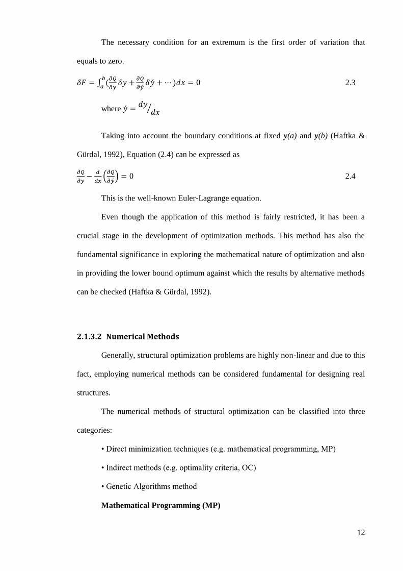
12

The necessary condition for an extremum is the first order of variation that

equals to zero.

∫

‎2.3

where

⁄

Taking into account the boundary conditions at fixed y(a) and y(b) (Haftka &

Gürdal, 1992), Equation (2.4) can be expressed as

(

) ‎2.4

This is the well-known Euler-Lagrange equation.

Even though the application of this method is fairly restricted, it has been a

crucial stage in the development of optimization methods. This method has also the

fundamental significance in exploring the mathematical nature of optimization and also

in providing the lower bound optimum against which the results by alternative methods

can be checked (Haftka & Gürdal, 1992).

2.1.3.2 Numerical Methods

Generally, structural optimization problems are highly non-linear and due to this

fact, employing numerical methods can be considered fundamental for designing real

structures.

The numerical methods of structural optimization can be classified into three

categories:

• Direct minimization techniques (e.g. mathematical programming, MP)

• Indirect methods (e.g. optimality criteria, OC)

• Genetic Algorithms method

Mathematical Programming (MP)

13

One of the most well-liked optimum search techniques formulated in 1950s was

Mathematical programming (MP) (Heyman, 1951). MP is a stage-by-stage search

approach concerning iterative processes and every iteration has two main steps:

a) Differentiating the value the objective function is assigned to and its gradients

considering all design variables,

b) Calculation of a change of the design variable that would result in a reduction

of the objective function.

Steps a) and b) needs to be recurred until a local minimum of the objective

function is reached.

In the early days, the mathematical programming method was solely restricted to

linear problems where the constraints and objective functions happen to be linear

functions of design variables. Since 1960, many algorithms of nonlinear programming

techniques have been developed such as nonlinear programming (NLP) (Schmit, 1960),

feasible direction (Zoutendijk, 1960), gradient projection (Rosen, 1961) and penalty

function method (Fiacco & McCormick, 1968). Simultaneously, approximation

techniques which employ the standard linear programming to address nonlinear

problems (Arora, 1993) have been studied, such as sequential linear programming.

One of the main advantages of MP methods is that MP methods are able to be

employed in most problems of structural optimization field. On the other hand, the main

disadvantage of MP methods is that as the number of design variables and constraints

increases, the cost of computing derivatives becomes expensive.

Optimality Criteria

Optimality criteria are the necessary conditions for minimality of the objective

function and these can be derived by either using variational methods or extremum

principles of mechanics. Optimality criteria (OC) method was analytically formulated

by Prager and his co-workers in 1960s (Prager & Taylor, 1968; Prager & Shield, 1968).

14

It was later developed numerically and became a widely accepted structural

optimization method (Venkayya, Khot, & Reddy, 1968).

OC methods can be divided into two types. One type is rigorous mathematical

statements such as the Kuhn-Tucker conditions. The other is algorithms used to resize

the structure for satisfying the optimality criterion. Different optimization problems

require different forms of the optimality criterion.

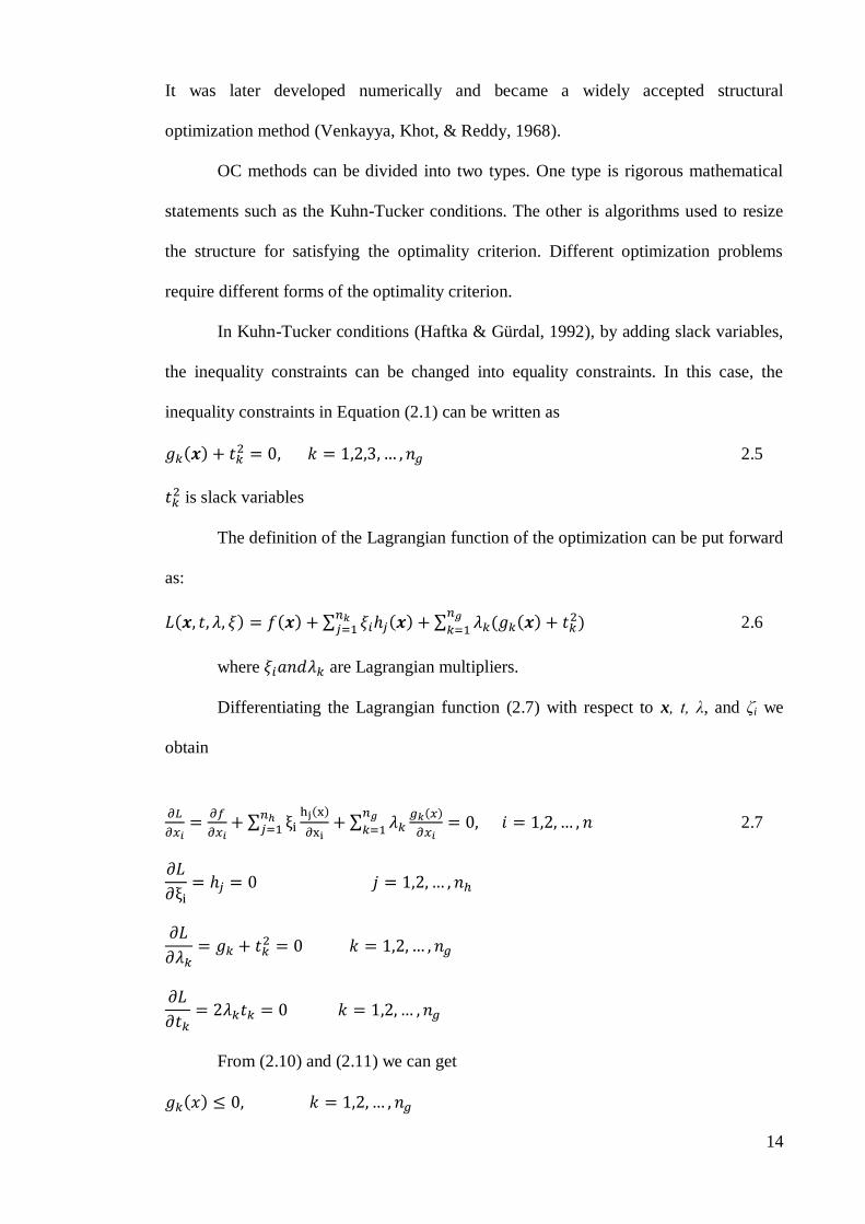
In Kuhn-Tucker conditions (Haftka & Gürdal, 1992), by adding slack variables,

the inequality constraints can be changed into equality constraints. In this case, the

inequality constraints in Equation (2.1) can be written as

‎2.5

is slack variables

The definition of the Lagrangian function of the optimization can be put forward

as:

∑ ∑

‎2.6

where are Lagrangian multipliers.

Differentiating the Lagrangian function (2.7) with respect to x, t, λ, and ζi we

obtain

∑

∑

‎2.7

From (2.10) and (2.11) we can get

15

This implies that when an inequality constraint is not active, the Lagrangian

multiplier associated with the constraint is zero.

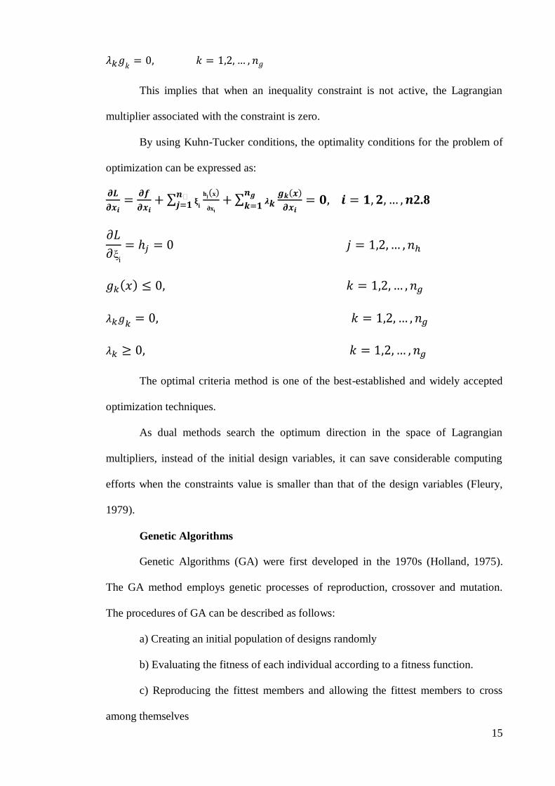
By using Kuhn-Tucker conditions, the optimality conditions for the problem of

optimization can be expressed as:

∑

∑

‎2.8

The optimal criteria method is one of the best-established and widely accepted

optimization techniques.

As dual methods search the optimum direction in the space of Lagrangian

multipliers, instead of the initial design variables, it can save considerable computing

efforts when the constraints value is smaller than that of the design variables (Fleury,

1979).

Genetic Algorithms

Genetic Algorithms (GA) were first developed in the 1970s (Holland, 1975).

The GA method employs genetic processes of reproduction, crossover and mutation.

The procedures of GA can be described as follows:

a) Creating an initial population of designs randomly

b) Evaluating the fitness of each individual according to a fitness function.

c) Reproducing the fittest members and allowing the fittest members to cross

among themselves

16

d) Developing a new generation with member having higher degree of desirable

characteristics than the parent generation

e) Repeating the procedure until reaching a near optimum solution

Although the GA method may not yet be as popular as MP or OC method, this

method has merits of being reliable and robust (Haftka & Gürdal, 1992; Nagendra,

Haftka, & Giirdal, 1993).

2.2 Structural Topological Optimization

Considering the numerical methods in structural optimization design, the

research begins with element stiffness design through shape and geometric, and then

moves to topology optimization design. Similarly, at the conceptual stage, a main

impact on the structural efficiency is carried out by the topology and the structure shape.

This normally is the case in the sense of stress/volume or stiffness/volume ratio. If there

exists an error in the topology or the structural shape, any amount of cross-sections and

fine-tuning will not compensate for this (Olhoff, Bendsoe, & Rasmussen, 1991).

With the development of high-speed computers, the topology optimization

method using numerical approach has been growing quickly (Haftka & Grandhi, 1986;

Kirsch, 1989; Rozvany, 1995). In the first attempt in performing numerical approaches,

a domain of material was used and boundary conditions and external loads were applied

to this domain. Afterwards, the optimization algorithm proceeds with removing the

ineffectual material to get the best structural optimization. In most cases, the objective

function for topology optimization problems is often the compliance (Taylor, 1977).

Generally, structural topology optimization could be considered as a material

distribution problem. Topology optimization can be divided into two classes; for

discrete and continuous structures. Early solutions for topology optimization of discrete

structures were put forward by Don et al. (Dorn, Gomory, & Greenberg, 1964); Dobbs

17

and Felton (Dobbs & Felton, 1969). Afterwards, instances of applying the concept to

large-scale structures have been given by Zhou and Rozvany (Zhou & Rozvany, 1991).

The continuum is normally separated into suitable finite elements. Each element carries

intrinsic structural features. They are reviewed in the following sections.

2.2.1 Topology optimization for Discrete Structures

Topology optimization for discrete structures has mainly been employed for

structures like trusses and frames. Its core concept is figuring out the optimal number,

mutual connectivity and position of the structural members. In other word, it can be

seen as exploring the optimal connectivity and spatial order of the bars.

Based on the survey by Topping (Bendsøe & Mota Soares, 1993), topology

optimization method for discrete structures can be categorized into three classes:

a) Geometric approach

b) Hybrid approach

c) Ground structure approach

2.2.1.1 Geometric Approach

In the geometric approach, the design variables are the properties of cross-

section and the coordinates of joints. While the optimization process is in progress, the

number of connecting members and joints are fixed as some joints are allowed to

coalesce.

2.2.1.2 Hybrid Approach

In the hybrid approach, the design variables are divided into size design

variables and geometrical design variables and are separated in the design space. While

the optimization process is in progress, firstly, the element size is changed while the

18

topology is kept unchanged; after that, the searching begins for the optimum position of

the element nodes.

2.2.1.3 Ground Structure Approach

In this method, a ground structure is considered as a dense group of nodes and a

number of potential connections between the nodes. While the optimization process is

in progress, the size and the number of connecting elements are altered, however, the

position and the number of nods are kept intact. If the section area of elements is

decreased to zero during the optimization process, the elements are deemed as non-

existent and the topology is changed accordingly.

A notable advantage of the ground structure approach method is that the design

domain is fixed thus the problem of mesh regeneration can be evaded.

2.2.2 Topology Optimization for Continuous Structures

Continuum topology optimization seeks to determine the inner holes and also

the internal and external boundaries (Bendsøe & Sigmund, 2003; Huang & Xie, 2010;

Krog & Olhoff, 1999), or as it came in reference (Huang & Xie, 2010), topology

optimization of continuum structures will determine the optimal designs through

indicating the best geometries and cavity locations in the design domain.

It also should be mentioned that whilst the shape and size structural optimization

still have applications in various industries, but technically and economically aspects

have made the topology optimization of continuum structures the most common

approach. It is due to the freedom of crating entirely efficient and new conceptual

designs that topology optimization of continuous structures makes in comparison to the

shape and size structural optimization. It also should be added that this technique has a

19

wide range of applications, from large-scale structures such as buildings and bridges to

micro and nano-levels (Huang & Xie, 2010).

As it was mentioned earlier, numerical methods have a vast usage in topology

optimization especially for topology optimization of continuum structures. The first

work published in this area was by Bendsoe and Kikuchi in 1989 (Bendsøe & Kikuchi,

1989). Numerical methods mostly have its grounds in Finite Element Analysis (FEA)

that discrete the design domain into a fine mesh element. In such situation, finding the

topology of the structure by identifying each single point in the design domain and

whether there should be material (solid element) or not (void element) could be seen as

the optimization procedure.

According to the survey by Topping (Bendsøe & Mota Soares, 1993), topology

optimization method for continuum structures could be categorized into four classes as

mentioned as follow.

2.2.2.1 Heuristic Methods

Heuristic methods are those addressing structural optimization problems in a

less mathematical but more intuitive way. Instead of complex mathematical

formulation, the heuristic methods are based on simple concepts or natural laws.

2.2.2.2 Evolutionary Structural Optimization Method (ESO)

The evolutionary structural method was initially put forward by Xie and Steven

(Xie & Steven, 1993; Xie & Steven, 1994). This method has its grounds in the notion of

removing the inefficient material from the structure slowly and/or moving the material

from the strongest to the weakest part of the structure gradually until the desired

optimum is achieved. The ESO approach offers a simple way to obtain optimum

20

designs using standard finite element analysis codes. Compared to other structural

optimization methods, the ESO approach is overwhelmingly interesting because of its

effectiveness and ease of use. During the last ten years, the capability of ESO to solve

numerous problems of shape, size and topology optimum designs for static and dynamic

problems has been proven in many instances (Rong, Xie, Yang, & Liang, 2001).

2.2.2.3 Homogenization Method

Compared to the Heuristic and ESO methods, the homogenization method is

more complex. This method is based on the mathematical theory of homogenization.

This theory was developed in the 1970’s (Babuska, 1976; Cioranescu & Paulin, 1979).

The homogenization method can be employed to discover the helpful features of the

equivalent homogenized material and are applicable to numerous areas of engineering

and physics. Since being firstly proposed for topology optimization in 1988 by

Bendsøeand Kikuchi (Bendsøe & Kikuchi, 1988), homogenization method has attracted

many researchers and design engineers. It has been used by industrial companies around

the world for product development, particularly in the automobile industry.

The homogenization approach has successfully been followed both in static and

dynamic problems with weighted constraints (Ma, Kikuchi, & Cheng, 1995; Tenek &

Hagiwara, 1993). With regard to the algorithm aspect, the homogenization method uses

traditional mathematical programming or optimality criteria as search techniques. The

advantages of homogenization method are precise theoretical basis and good

convergence behaviour. On the other hand, the disadvantage of homogenization method

is that difficulties associated with those traditional methods are magnified in the

homogenization method.

21

2.2.2.4 H/e-method

The h/e-method is a hybrid method. It is an abbreviation of the combination of

homogenization and evolutionary methods in various degrees. Bulman, Sienz and

Hinton (Bulman, Sienz, & Hinton, 2001) developed the constrained adaptive topology

optimization (CATO) algorithm, combined of two methods: the homogenization

method which is mathematically more rigorous and also the evolutionary method which

is more intuitive. Through a set of benchmarks, they systematically investigated the

performance of the algorithm for topology optimization. The results of the study show

that in general cases, the h/e CATO algorithms was very well comparable with the

homogenization method.

2.3 Topology Optimization Related to Vibration Problem

This section will explain the topology optimization related to vibration problems

as an application and category of structural optimization.

Improving the dynamic behaviour of a structure is very essential. For example,

minimizing the noise and vibration when the loading condition is known is a very

important consideration in a car body design. In this case and similar cases like this, it is

to treat the dynamic behaviour of the system as an object of the optimization process,

not as a constraint (Ma, Cheng, & Kikuchi, 1994).

On the other hand, one of the most challenging and difficult parts of applying

the topology optimization method is to develop sensible combinations of objective

functions and constraints. In the design of dynamic systems, For example, structural

vibration control is particularly a central consideration. On the other hand, the main idea

of the structural optimization is to obtain an optimal material layout of a load bearing

structure. But traditionally, these two have been considered independently, the structural

designers develops their designs according to stiffness and strength necessities and the

22

control designers constructs the control algorithm in order to decrease the dynamic

response of a structure (Kang, Wang, & Wang, 2009; Ou & Kikuchi, 1996). Here, the

means of “topology optimization related to vibration problem” is a simultaneously

consideration of structural vibration control and structural optimization.

Generally, topology optimization related vibration problems follows some aims

in concept. The first aim is that, it intends the specified structural eigenvalues to reach a

maximum. The second one is that, it aims at maximizing the distances of the specified

structural eigenfrequencies from a given frequency. The third aim is to optimize a

structure for the purpose of obtaining prescribed desired eigenfrequencies (Ma et al.,

1994). On the other hand, topology optimization for vibration problems can be

categorized in two main categories; with respect to free vibration and with respect to

forced vibration.

Eigenvalue optimization for free vibrations can be considered as one of the

initial applications of topology optimization method. This problem is important for the

design of structures and machines which are dependent on dynamic load. For example,

one may wish to maintain the eigenfrequencies of a structure away from the driving

frequency of an attached engine or one may wish to keep the fundamental

eigenfrequencies well above possible disturbance frequencies. Also, structures with

high fundamental eigenfrequency are inclined to be reasonably stiff for all conceivable

loads and therefore maximization of the fundamental frequency results in designs that

are also good for static loads (Bendsøe & Sigmund, 2003).

There are some important considerations involving Structural Dynamics

Modifications (SDM) and topology optimization related to vibration problem. Structural

dynamics modification (SDM) is extensively employed to alter mode shapes and/or

natural frequencies through the addition or the elimination of auxiliary members in

order to improve the dynamic response of a target structure. The differences of SDM

23

and topology for vibration problems can be summarized in two general factors. The first

one is that the application of SDM is modifying the existing structures for the next

generation design cycle. The second one is that SDM is used as a tool to remove the

non-smoothness of eigenvalues (Jung, Park, & Park, 2005).

As it has been mentioned in the previous parts, the main objective of the

topology optimization problem is to discover a material distribution which minimizes a

given objective functional, subjected to a set of constraints, achieved by a consistent

parameterization of the material properties in each part of the design domain. A natural

question is whether there exists or not material in a given point, which leads to a

discrete problem. It is well-known that this integer parameterization leads to numerical

difficulties, associated with the integer problem convergence (Bendsøe & Kikuchi,

1988; Bendsøe & Sigmund, 1999; Cardoso & Fonseca, 2003). Minimizing the vibration

effects of the dynamic response is an important goal for the structural vibration control,

and the effectively of the control depends on the weighting matrices (Molter, Fonseca,

Bottega, & Silveira, 2010).

There are two main numerical methods of topology optimization that are being

used in practical applications nowadays, including the Solid Isotropic Material with

Penalization (SIMP) method and Evolutionary Structural Optimization (ESO) method.

Bendsøe (1989) put forward the original idea of SIMP. ESO is the abbreviation for

“Evolutionary Structural Optimization”. ESO is a design method which has its roots in

the notion of eliminating inefficient material gradually from a structure. Bi-directional

Evolutionary Structural Optimization (BESO) is a new algorithm which has its grounds

in the improvement of ESO method (Huang & Xie, 2010).

Taking another perspective, structural optimization could be considered in two

main categories: one that is considering materials in level of macroscopic design and the

other in micromechanics subject. In macroscopic design, a macroscopic definition of

24

geometry is given by, for example, thicknesses or boundaries considered. On the other

hand, micromechanics are about studying the relation between microstructure and the

macroscopic behaviour of a composite material.

Since the focus of this project is related to the macroscopic structures, in the

following part, some of the works and researches in the area of structural optimization

with respect to vibration for macroscopic structures will be reviewed from the earliest

papers published in.

The first work in this scope has been done by Dias and Kikuchi in 1992 (Diaz &

Kikuchi, 1992). They considered topology optimization with reference to

eigenfrequencies of structural vibration. The concept of their work was maximizing a

natural frequency of a structure and presenting a strategy to discover its topology and

shape. The method they used is homogenization method that was applied for a two

dimensional, plane elasticity problem for a disk in which through a prescribed of

material, an offered structure is reinforced.

Ma et al. (Ma et al., 1994) defined a mean eigenvalue equivalent to the multiple

eigenvalues of a structure, and then according to the notion of Optimal Material

Distribution (OMD),three types of optimization problems was considered for arriving at

the desired eigenvalues. They obtained desired eigenvalues for maximization of the

particular structural eigenvalues, the amplification of the distances of the specified

structural eigenvalues from a given frequency, and the optimization of the structure to

achieve prescribed eigenvalues.

Zhao et al. (Zhao, Steven, & Xie, 1998) propose a method to resolve the natural

frequency optimization of membrane vibration by using of evolutionary method

according to the finite element method and evolutionary standard. Founded on the

general finite element formulation along with the energy conservation principle of

structural eigenvalue problem, they defined a contribution factor of an element for a

25

discretized system. From a physical point of view, the contribution factor of an element

entails that an element has contributed directly to the natural frequency of the structure.

As an instance, they applied their method on a square membrane with four sides fixed.

Generally vibration optimization amounts to the optimization of eigenvalues in

free vibration problems. But there are some works that are done for optimization of

structures which are subject to periodic loading. Jog (Jog, 2002) has done a work for the

minimization of vibrations of structures which were subjected to periodic loading with

respect to two kinds of measures, one global and the other local. Means of Global

measures was to reduce the vibration in an overall sense. It can be termed as “dynamic

compliance”, and thus, it has important implications for the noise reduction of a

structure. Means of Local measures is the reduction of the vibration at a local point.

The aim here is to minimize the frequency response amplitude at a given point in the

structure, although it might increase the amplitudes at other points in the structure. Both

measures are based on reducing the vibration level by moving the natural frequencies

and the driving frequencies away from one another. By presenting some numerical

examples, it turned out that the structure of dynamic compliance optimization problem

is very similar to the structure of the static compliance optimization problem.

Jensen et al. (Jensen & Pedersen, 2006) worked on structures with two material

components . They used finite element analysis and material distribution method of

topology optimization to maximize dividing of two nearby eigenvalues in structures.

They used two different formulations to maximize the separation of the eigenvalues. In

the formulation that was out forward firstly, the objective of the optimization was

considered as the maximum difference in the frequencies. The second formulation is

maximizing the ratios of two adjacent eigenvalues. The methods are considered for

optimal design of 1D and 2D structures.

26

An integrated design procedure was introduced by Molter et al. (Molter,

Fonseca, Bottega, Otávio, & Silveira, 2010) for topology optimization and structural

control system. In his work, a structural topology optimization methodology derived

from the notion of optimizing the material density distribution is presented for a

cantilever beam, which includes an optimal control design for vibrations reduction. The

concept of this work is to design the structure and controls simultaneously, meanings

that the cost function includes not only the strain energy, but also the control energy. A

continuum finite element modelling is applied to simulate the dynamic characteristics of

the structure and the modal basis is used to derive an optimal control.

Whilst the nature of dynamic problems is non-linear, for simplicity, dynamic

problems are usually solved using of linear methods. Yoon (Yoon, 2010) used topology

optimization rooted in the internal element connectivity parameterization (I-ECP) for

non-linear dynamic problems. The I-ECP method has more advantages to solve non-

linear problems because it uses topology optimization method to solve non-linear

dynamic problems. Such methods are based on standard density and they are influenced

by element instability, numerical difficulties, and localized vibration modes. However,

the I-ECP method avoids element instability and a new patch mass model in the I-ECP

formulation is offered for controlling the problem of localized vibration modes.

All the works have been reviewed here were based on using topology

optimization for solving the vibration problems. However, since all these works were

done for the design stage, the manufacturability was not a condition of their work. In the

present work, one of the most important conditions of the work was the

manufacturability of the new structure to be appropriate for the industry.

27

Chapter Three

3 Methodology

The following chapter describes the methods used in this research. Here, three

separate studies are conducted and the results of each part are used for the rest of the

research. At first, an experimental modal analysis and an ODS measurement are

conducted on the structure, and the results are used to validate the finite-element model.

Optimization is then done based on this finite-element model to optimize the assumed

structure.

The methods employed in these parts are described in the next section.

3.1 Experimental Modal Analysis (EMA)

The Experimental Modal Analysis (EMA) aims at identifying the dynamic

properties of a structure. These properties are derived usually from acquired time

domain signals. They can also be derived by using the frequency functions that are

computed based on time domain signals. A multi-channel FFT (Fast Fourier Transform)

analyser is often utilized to collect these signals and to measure the vibration response

of a structure in multiple points and directions (DOFs). The vibration signals are

amplified, digitized and stored in the analyser’s for further post-processing. After that,

the modal parameters can be calculated from these signals. Experimental modal data are

also called modal testing.

Modal data of a structure consists of natural frequencies, damping factor and

mode shapes. These data can be measured experimentally from Frequency Response

Function (FRF) data between one or more reference positions, called Degree of

Freedom (DOF). Each DOF has a direction and a point. To perform an accurate EMA,

sufficient numbers of DOFs are needed.

28

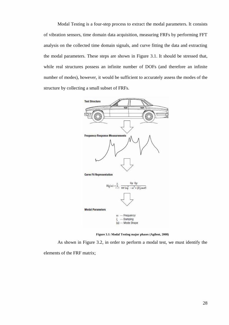
Modal Testing is a four-step process to extract the modal parameters. It consists

of vibration sensors, time domain data acquisition, measuring FRFs by performing FFT

analysis on the collected time domain signals, and curve fitting the data and extracting

the modal parameters. These steps are shown in Figure ‎3.1. It should be stressed that,

while real structures possess an infinite number of DOFs (and therefore an infinite

number of modes), however, it would be sufficient to accurately assess the modes of the

structure by collecting a small subset of FRFs.

Figure ‎3.1: Modal Testing major phases (Agilent, 2008)

As shown in Figure ‎3.2, in order to perform a modal test, we must identify the

elements of the FRF matrix;

29

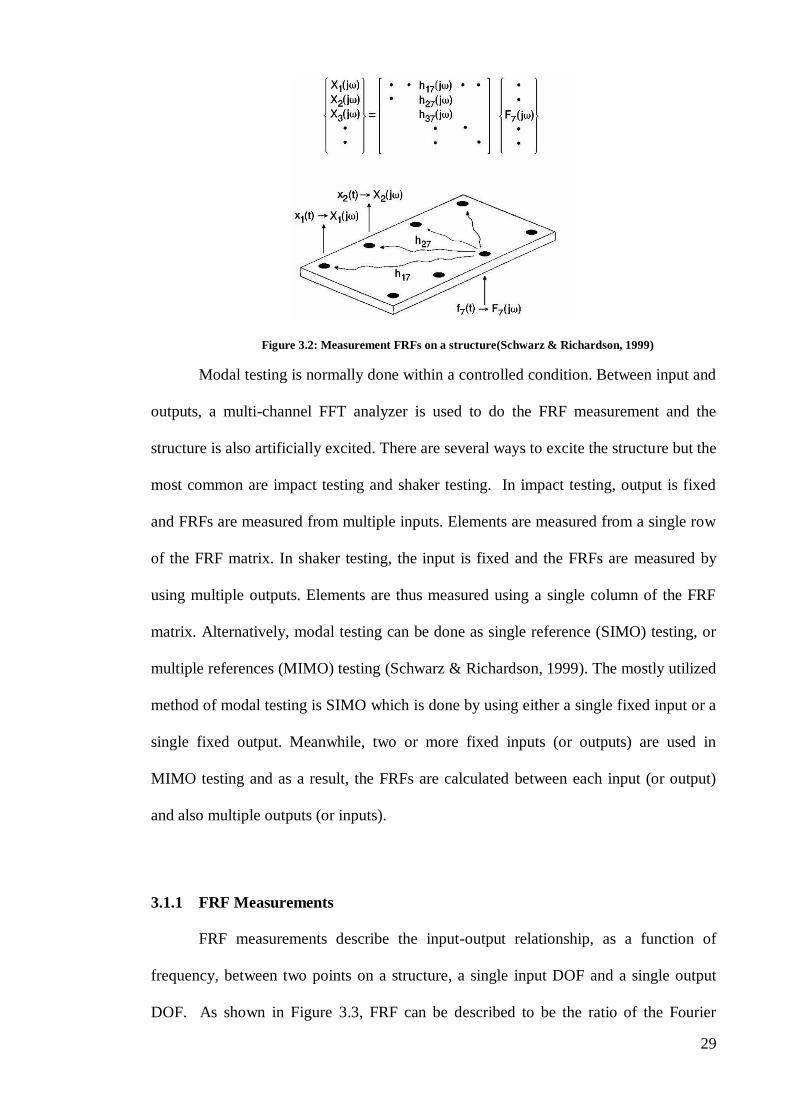
Figure ‎3.2: Measurement FRFs on a structure(Schwarz & Richardson, 1999)

Modal testing is normally done within a controlled condition. Between input and

outputs, a multi-channel FFT analyzer is used to do the FRF measurement and the

structure is also artificially excited. There are several ways to excite the structure but the

most common are impact testing and shaker testing. In impact testing, output is fixed

and FRFs are measured from multiple inputs. Elements are measured from a single row

of the FRF matrix. In shaker testing, the input is fixed and the FRFs are measured by

using multiple outputs. Elements are thus measured using a single column of the FRF

matrix. Alternatively, modal testing can be done as single reference (SIMO) testing, or

multiple references (MIMO) testing (Schwarz & Richardson, 1999). The mostly utilized

method of modal testing is SIMO which is done by using either a single fixed input or a

single fixed output. Meanwhile, two or more fixed inputs (or outputs) are used in

MIMO testing and as a result, the FRFs are calculated between each input (or output)

and also multiple outputs (or inputs).

3.1.1 FRF Measurements

FRF measurements describe the input-output relationship, as a function of

frequency, between two points on a structure, a single input DOF and a single output

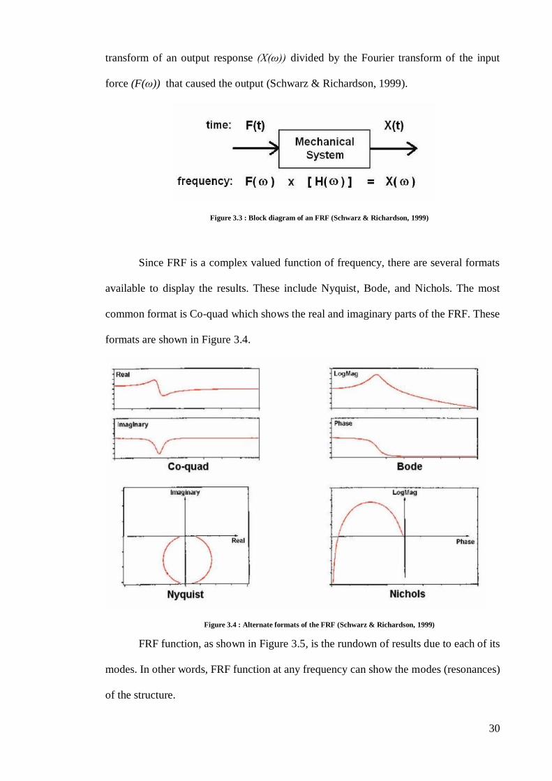
DOF. As shown in Figure ‎3.3, FRF can be described to be the ratio of the Fourier

30

transform of an output response (X(ω)) divided by the Fourier transform of the input

force (F(ω)) that caused the output (Schwarz & Richardson, 1999).

Figure ‎3.3 : Block diagram of an FRF (Schwarz & Richardson, 1999)

Since FRF is a complex valued function of frequency, there are several formats

available to display the results. These include Nyquist, Bode, and Nichols. The most

common format is Co-quad which shows the real and imaginary parts of the FRF. These

formats are shown in Figure ‎3.4.

Figure ‎3.4 : Alternate formats of the FRF (Schwarz & Richardson, 1999)

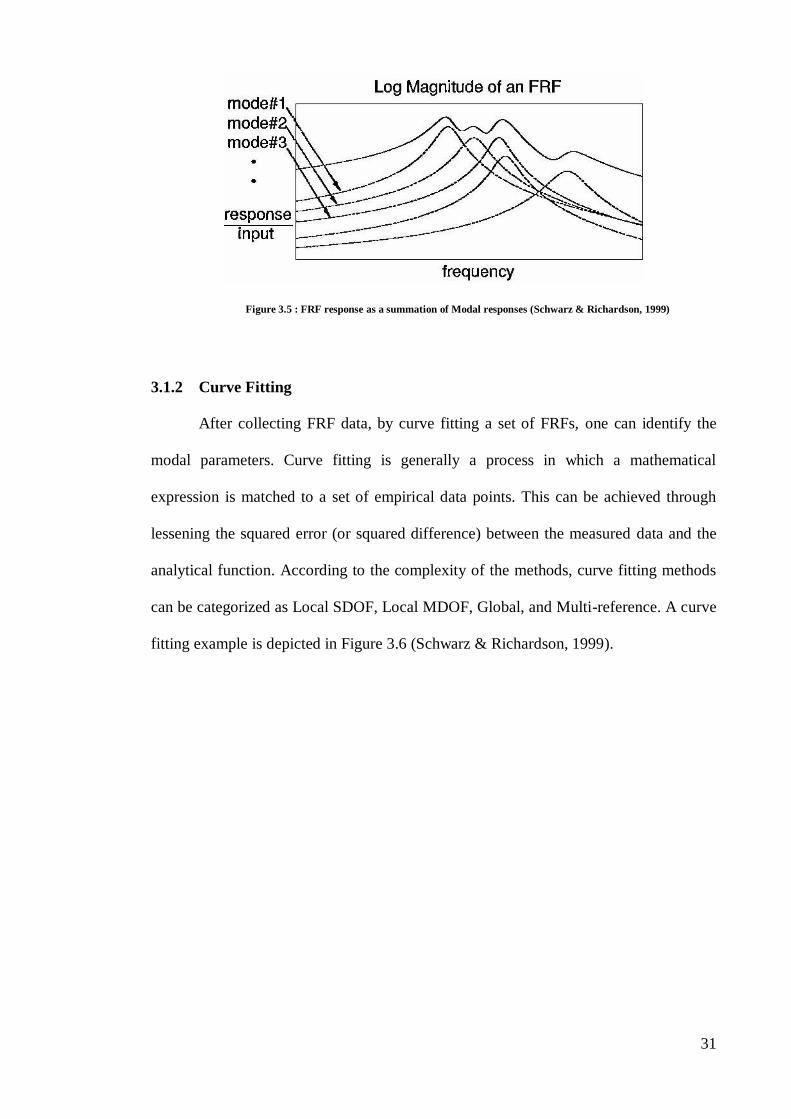
FRF function, as shown in Figure ‎3.5, is the rundown of results due to each of its

modes. In other words, FRF function at any frequency can show the modes (resonances)

of the structure.

31

Figure ‎3.5 : FRF response as a summation of Modal responses (Schwarz & Richardson, 1999)

3.1.2 Curve Fitting

After collecting FRF data, by curve fitting a set of FRFs, one can identify the

modal parameters. Curve fitting is generally a process in which a mathematical

expression is matched to a set of empirical data points. This can be achieved through

lessening the squared error (or squared difference) between the measured data and the

analytical function. According to the complexity of the methods, curve fitting methods

can be categorized as Local SDOF, Local MDOF, Global, and Multi-reference. A curve

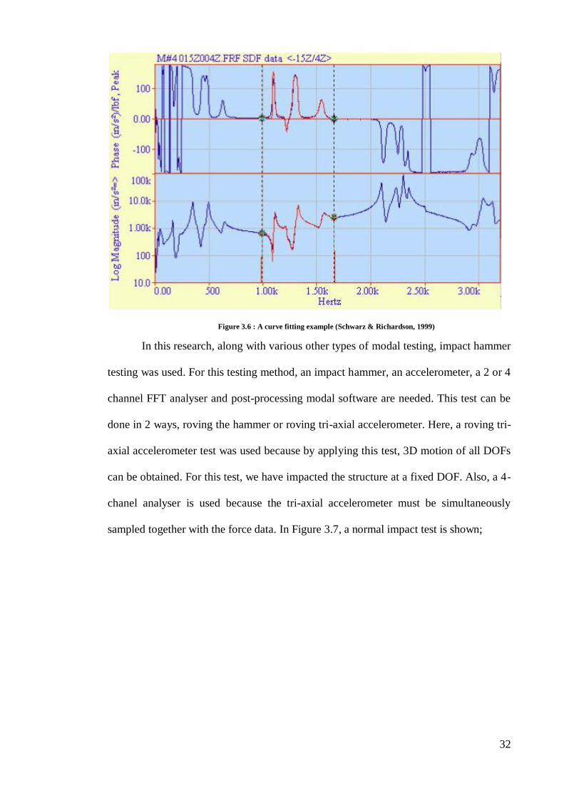
fitting example is depicted in Figure ‎3.6 (Schwarz & Richardson, 1999).

32

Figure ‎3.6 : A curve fitting example (Schwarz & Richardson, 1999)

In this research, along with various other types of modal testing, impact hammer

testing was used. For this testing method, an impact hammer, an accelerometer, a 2 or 4

channel FFT analyser and post-processing modal software are needed. This test can be

done in 2 ways, roving the hammer or roving tri-axial accelerometer. Here, a roving tri-

axial accelerometer test was used because by applying this test, 3D motion of all DOFs

can be obtained. For this test, we have impacted the structure at a fixed DOF. Also, a 4-

chanel analyser is used because the tri-axial accelerometer must be simultaneously

sampled together with the force data. In Figure ‎3.7, a normal impact test is shown;

33

Figure ‎3.7 : Impact testing (Schwarz & Richardson, 1999)

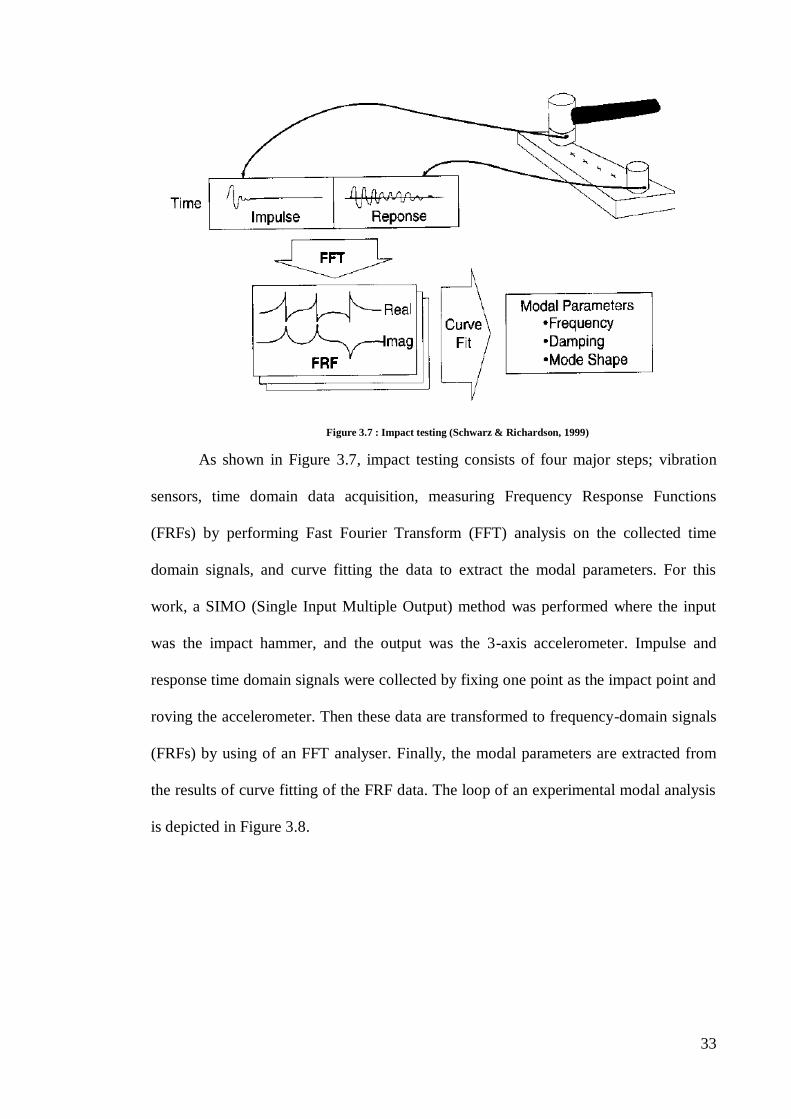
As shown in Figure ‎3.7, impact testing consists of four major steps; vibration

sensors, time domain data acquisition, measuring Frequency Response Functions

(FRFs) by performing Fast Fourier Transform (FFT) analysis on the collected time

domain signals, and curve fitting the data to extract the modal parameters. For this

work, a SIMO (Single Input Multiple Output) method was performed where the input

was the impact hammer, and the output was the 3-axis accelerometer. Impulse and

response time domain signals were collected by fixing one point as the impact point and

roving the accelerometer. Then these data are transformed to frequency-domain signals

(FRFs) by using of an FFT analyser. Finally, the modal parameters are extracted from

the results of curve fitting of the FRF data. The loop of an experimental modal analysis

is depicted in Figure 3.8.

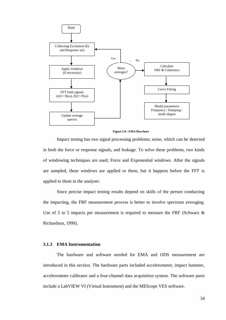
34

Figure ‎3.8 : EMA flowchart

Impact testing has two signal processing problems; noise, which can be detected

in both the force or response signals, and leakage. To solve these problems, two kinds

of windowing techniques are used; Force and Exponential windows. After the signals

are sampled, these windows are applied to them, but it happens before the FFT is

applied to them in the analyser.

Since precise impact testing results depend on skills of the person conducting

the impacting, the FRF measurement process is better to involve spectrum averaging.

Use of 3 to 5 impacts per measurement is required to measure the FRF (Schwarz &

Richardson, 1999).

3.1.3 EMA Instrumentation

The hardware and software needed for EMA and ODS measurement are

introduced in this section. The hardware parts included accelerometer, impact hammer,

accelerometer calibrator and a four-channel data acquisition system. The software parts

include a LabVIEW VI (Virtual Instrument) and the MEScope VES software.

Start

Collecting Excitation f(t)

and Response x(t)

And

Apply windows (if necessary)

FFT both signals

x(t)=>X(ω), f(t)=>F(ω)

Update average spectra

More averages?

Calculate

FRF & Coherence

Curve Fitting

Modal parameters Frequency / Damping /

mode shapes

Yes No

35

3.1.3.1 Accelerometer

An accelerometer is a piezoelectric transducer. Transducers are instruments that

are used for sensing force and motion. The piezoelectric transducers are the most widely

used for modal testing among different existing types because of their wide frequency

and dynamic range, good linearity and durability. When subjected to vibration, a

piezoelectric transducer generates an electrical output. A crystal element that creates an

electrical charge when mechanically strained is in fact the main cause of this. When the

accelerometer vibrates, the internal mass in the assembly applies a force to the crystal

element which is proportional to the acceleration. This relationship is simply Newton’s

law: force equals mass times acceleration (Agilent, 2008).

There are also some operating specifications that should be considered when

using an accelerometer. These are sensitivity, resonant frequency, temperature range

and shock rating. A quality accelerometer enjoys high sensitivity, a wide frequency

range and small mass. The unit for sensitivity is mV/G. The resonant frequency of the

transducer is a function of the mass and stiffness of the transducer, and the stiffness of

the mounting method used. Therefore, the frequency range of the test should be within

the linear range below the resonance of the transducer. Generally, the usable frequency

range is around one-third of the resonance frequency which is required to achieve a

linear frequency response. It is shown in Figure 3.9 (Agilent, 2008; Ramli, 1998).

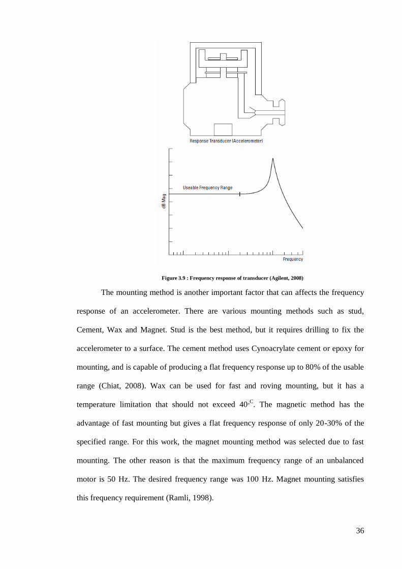
36

Figure ‎3.9 : Frequency response of transducer (Agilent, 2008)

The mounting method is another important factor that can affects the frequency

response of an accelerometer. There are various mounting methods such as stud,

Cement, Wax and Magnet. Stud is the best method, but it requires drilling to fix the

accelerometer to a surface. The cement method uses Cynoacrylate cement or epoxy for

mounting, and is capable of producing a flat frequency response up to 80% of the usable

range (Chiat, 2008). Wax can be used for fast and roving mounting, but it has a

temperature limitation that should not exceed 40oC. The magnetic method has the

advantage of fast mounting but gives a flat frequency response of only 20-30% of the

specified range. For this work, the magnet mounting method was selected due to fast

mounting. The other reason is that the maximum frequency range of an unbalanced

motor is 50 Hz. The desired frequency range was 100 Hz. Magnet mounting satisfies

this frequency requirement (Ramli, 1998).

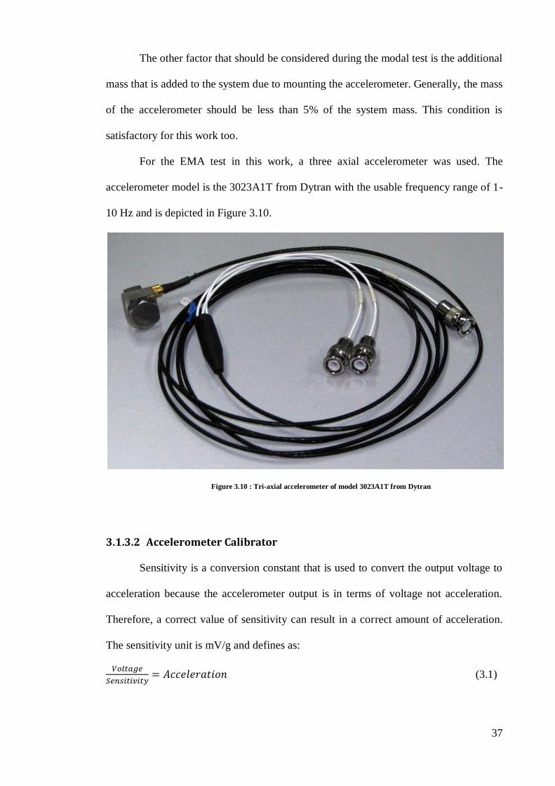
37

The other factor that should be considered during the modal test is the additional

mass that is added to the system due to mounting the accelerometer. Generally, the mass

of the accelerometer should be less than 5% of the system mass. This condition is

satisfactory for this work too.

For the EMA test in this work, a three axial accelerometer was used. The

accelerometer model is the 3023A1T from Dytran with the usable frequency range of 1-

10 Hz and is depicted in Figure 3.10.

Figure ‎3.10 : Tri-axial accelerometer of model 3023A1T from Dytran

3.1.3.2 Accelerometer Calibrator

Sensitivity is a conversion constant that is used to convert the output voltage to

acceleration because the accelerometer output is in terms of voltage not acceleration.

Therefore, a correct value of sensitivity can result in a correct amount of acceleration.

The sensitivity unit is mV/g and defines as:

(3.1)

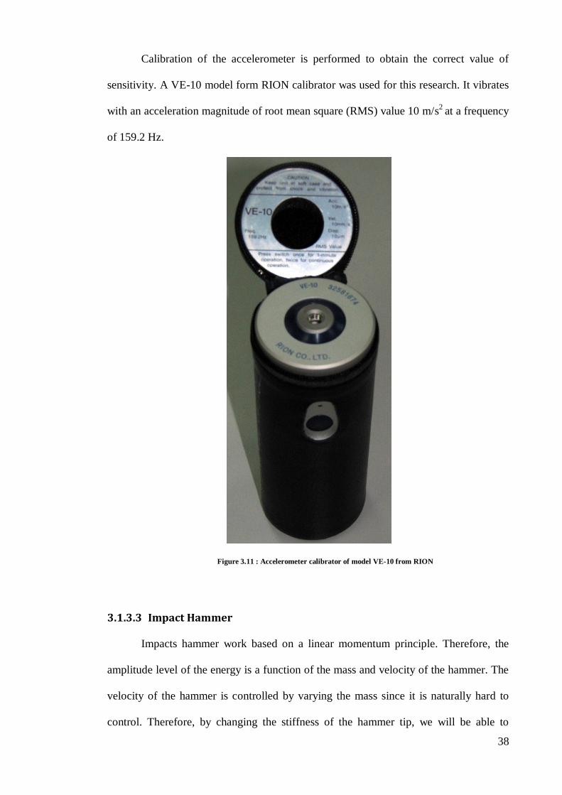
38

Calibration of the accelerometer is performed to obtain the correct value of

sensitivity. A VE-10 model form RION calibrator was used for this research. It vibrates

with an acceleration magnitude of root mean square (RMS) value 10 m/s2

at a frequency

of 159.2 Hz.

Figure ‎3.11 : Accelerometer calibrator of model VE-10 from RION

3.1.3.3 Impact Hammer

Impacts hammer work based on a linear momentum principle. Therefore, the

amplitude level of the energy is a function of the mass and velocity of the hammer. The

velocity of the hammer is controlled by varying the mass since it is naturally hard to

control. Therefore, by changing the stiffness of the hammer tip, we will be able to

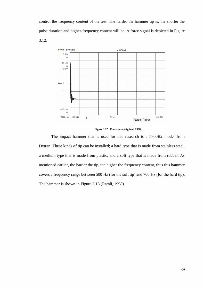
39

control the frequency content of the test. The harder the hammer tip is, the shorter the

pulse duration and higher-frequency content will be. A force signal is depicted in Figure

3.12.

Figure ‎3.12 : Force pulse (Agilent, 2008)

The impact hammer that is used for this research is a 5800B2 model from

Dytran. Three kinds of tip can be installed; a hard type that is made from stainless steel,

a medium type that is made from plastic, and a soft type that is made from rubber. As

mentioned earlier, the harder the tip, the higher the frequency content, thus this hammer

covers a frequency range between 500 Hz (for the soft tip) and 700 Hz (for the hard tip).

The hammer is shown in Figure 3.13 (Ramli, 1998).

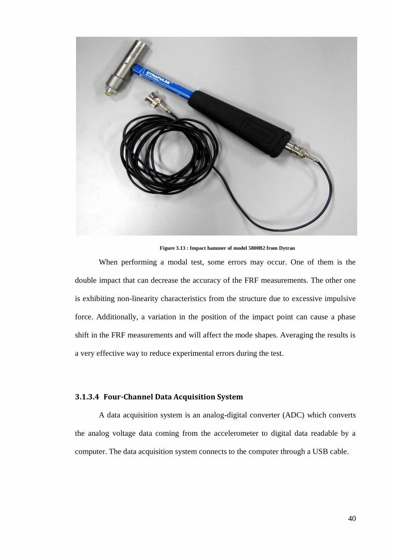
40

Figure ‎3.13 : Impact hammer of model 5800B2 from Dytran

When performing a modal test, some errors may occur. One of them is the

double impact that can decrease the accuracy of the FRF measurements. The other one

is exhibiting non-linearity characteristics from the structure due to excessive impulsive

force. Additionally, a variation in the position of the impact point can cause a phase

shift in the FRF measurements and will affect the mode shapes. Averaging the results is

a very effective way to reduce experimental errors during the test.

3.1.3.4 Four-Channel Data Acquisition System

A data acquisition system is an analog-digital converter (ADC) which converts

the analog voltage data coming from the accelerometer to digital data readable by a

computer. The data acquisition system connects to the computer through a USB cable.

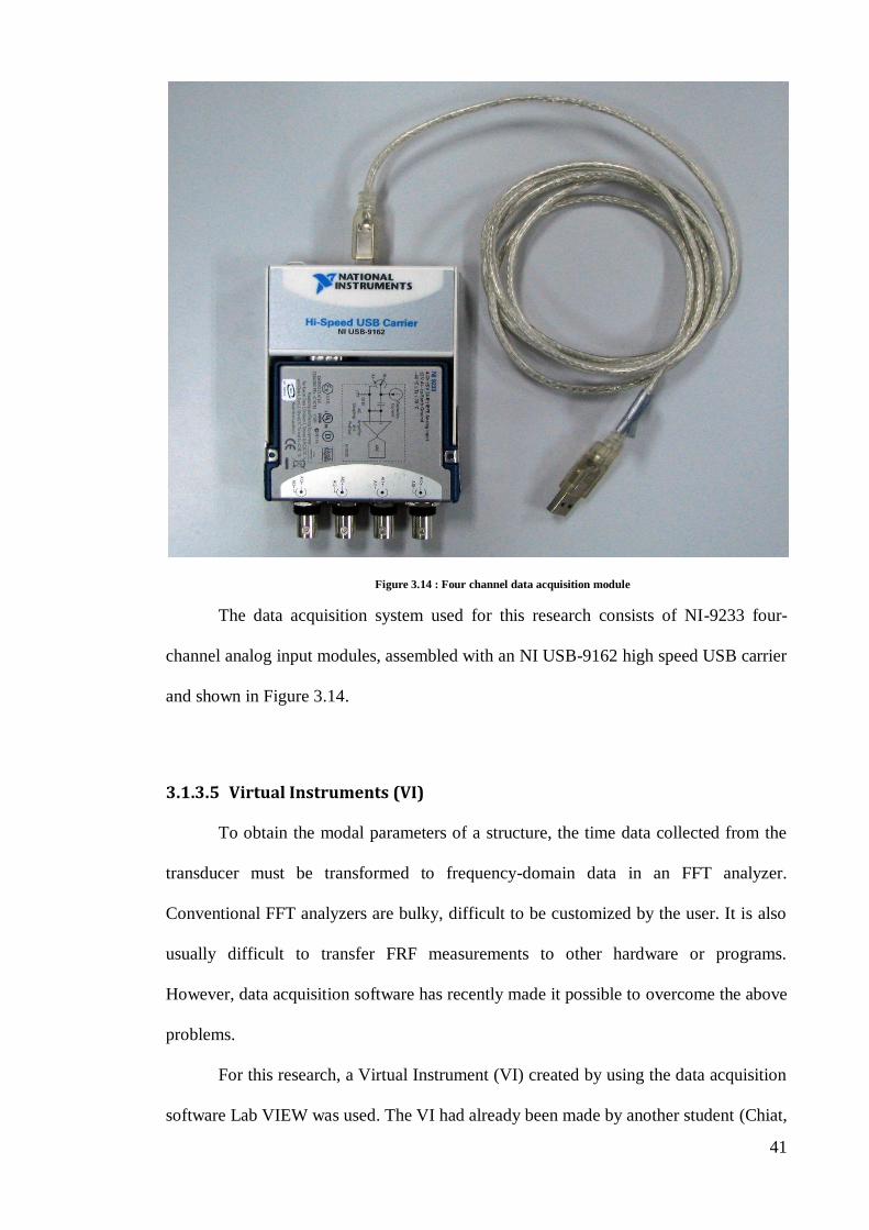
41

Figure ‎3.14 : Four channel data acquisition module

The data acquisition system used for this research consists of NI-9233 four-

channel analog input modules, assembled with an NI USB-9162 high speed USB carrier

and shown in Figure 3.14.

3.1.3.5 Virtual Instruments (VI)

To obtain the modal parameters of a structure, the time data collected from the

transducer must be transformed to frequency-domain data in an FFT analyzer.

Conventional FFT analyzers are bulky, difficult to be customized by the user. It is also

usually difficult to transfer FRF measurements to other hardware or programs.

However, data acquisition software has recently made it possible to overcome the above

problems.

For this research, a Virtual Instrument (VI) created by using the data acquisition

software Lab VIEW was used. The VI had already been made by another student (Chiat,

42

2008) and was used for this research. This FRF-analyzer VI includes a front panel and a

block diagram. The front panel contains controls and indicators and is the user interface.

The block diagram contains graphical programming codes that control the front panel.

The block diagram can be found in the reference (Chiat, 2008).

To be able to use the FRF analyzer VI, some initial configuration in the block

diagram needs to be set as seen in Table 3.1 and Figure 3.15 to Figure 3.17.

Table ‎3.1 : Initial configurations in block diagram of FRF-analyzer VI (Chiat, 2008)

LabVIEW module Parameter Features

DAQ

Sampling rate No. of digitized readings sampled in one second from

analog data.

No. of samples No. of samples to be read.

Sensitivity Calibrated sensitivity of accelerometer and impact

hammer.

Trigger

Threshold value Data will be taken for FRF calculation starting from

when impact force exceeded this value.

No. of samples No. of output samples for FRF calculation, counted

from the moment the impact force exceeded threshold

value.

FRF No. of averages No. of averages needed for FRF calculation.

43

Figure ‎3.15 : DAQ configuration in block diagram of FRF-analyzer VI (Chiat, 2008)

Figure ‎3.16 : Trigger configuration in block diagram of FRF-analyzer VI (Chiat, 2008)

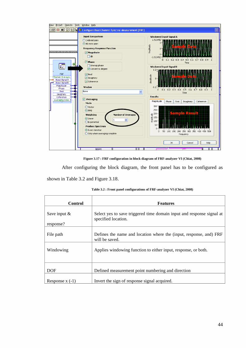
44

Figure ‎3.17 : FRF configuration in block diagram of FRF-analyzer VI (Chiat, 2008)

After configuring the block diagram, the front panel has to be configured as

shown in Table 3.2 and Figure 3.18.

Table ‎3.2 : Front panel configurations of FRF-analyzer VI (Chiat, 2008)

Control Features

Save input &

response?

Select yes to save triggered time domain input and response signal at

specified location.

File path Defines the name and location where the (input, response, and) FRF

will be saved.

Windowing

Applies windowing function to either input, response, or both.

DOF Defined measurement point numbering and direction

Response x (-1) Invert the sign of response signal acquired.

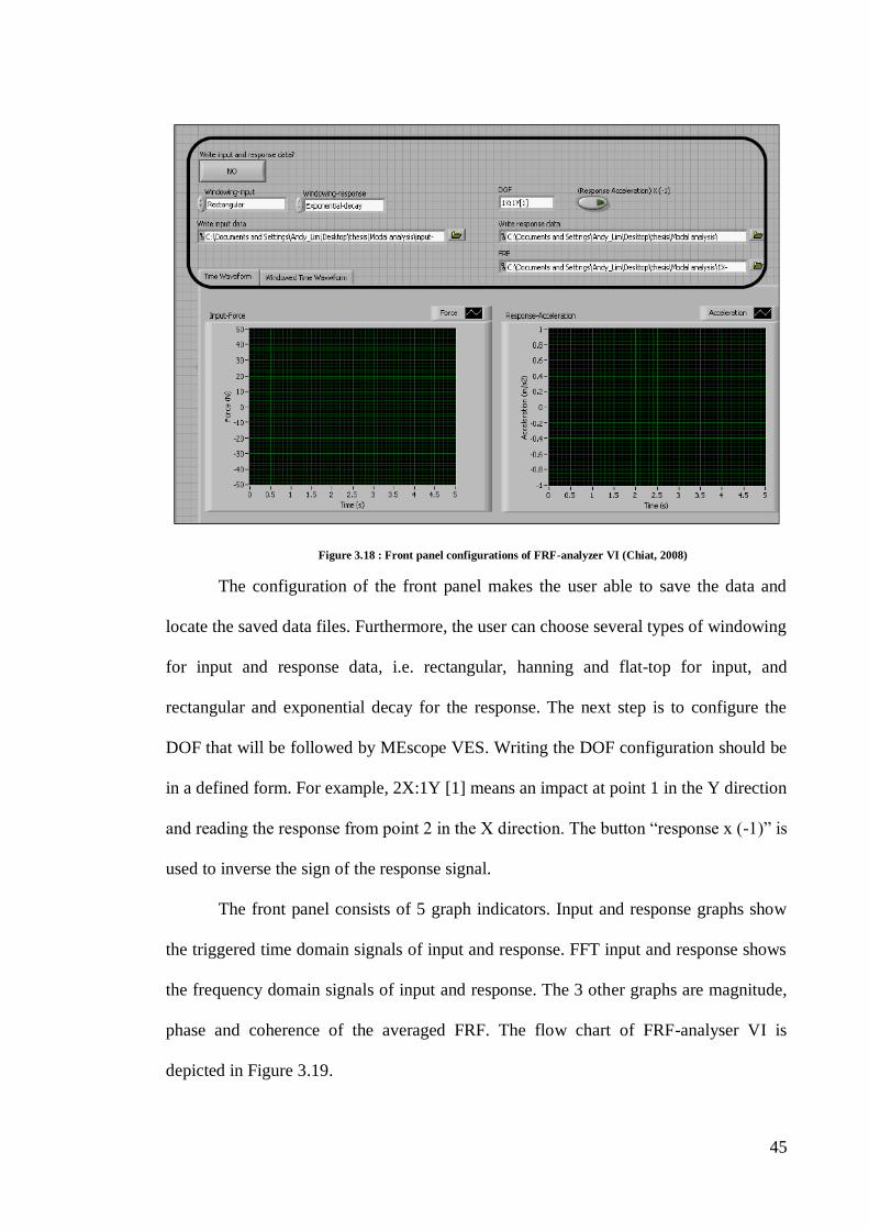
45

Figure ‎3.18 : Front panel configurations of FRF-analyzer VI (Chiat, 2008)

The configuration of the front panel makes the user able to save the data and

locate the saved data files. Furthermore, the user can choose several types of windowing

for input and response data, i.e. rectangular, hanning and flat-top for input, and

rectangular and exponential decay for the response. The next step is to configure the

DOF that will be followed by MEscope VES. Writing the DOF configuration should be

in a defined form. For example, 2X:1Y [1] means an impact at point 1 in the Y direction

and reading the response from point 2 in the X direction. The button “response x (-1)” is

used to inverse the sign of the response signal.

The front panel consists of 5 graph indicators. Input and response graphs show

the triggered time domain signals of input and response. FFT input and response shows

the frequency domain signals of input and response. The 3 other graphs are magnitude,

phase and coherence of the averaged FRF. The flow chart of FRF-analyser VI is

depicted in Figure 3.19.

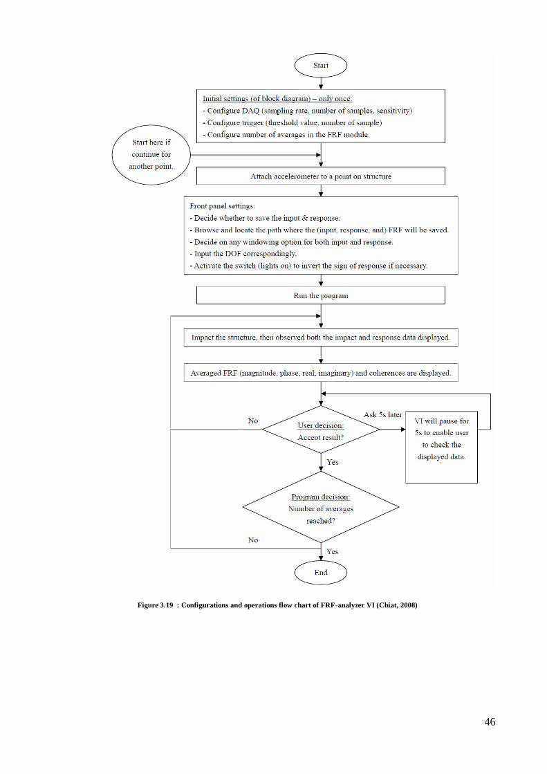
46

Figure ‎3.19 : Configurations and operations flow chart of FRF-analyzer VI (Chiat, 2008)

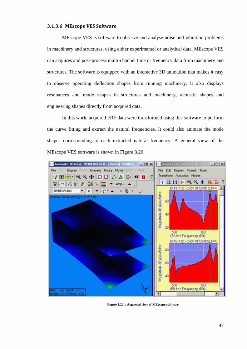
47

3.1.3.6 MEscope VES Software

MEscope VES is software to observe and analyse noise and vibration problems

in machinery and structures, using either experimental or analytical data. MEscope VES

can acquires and post-process multi-channel time or frequency data from machinery and

structures. The software is equipped with an interactive 3D animation that makes it easy

to observe operating deflection shapes from running machinery. It also displays

resonances and mode shapes in structures and machinery, acoustic shapes and

engineering shapes directly from acquired data.

In this work, acquired FRF data were transformed using this software to perform

the curve fitting and extract the natural frequencies. It could also animate the mode

shapes corresponding to each extracted natural frequency. A general view of the

MEscope VES software is shown in Figure 3.20.

Figure ‎3.20 : A general view of MEscope software

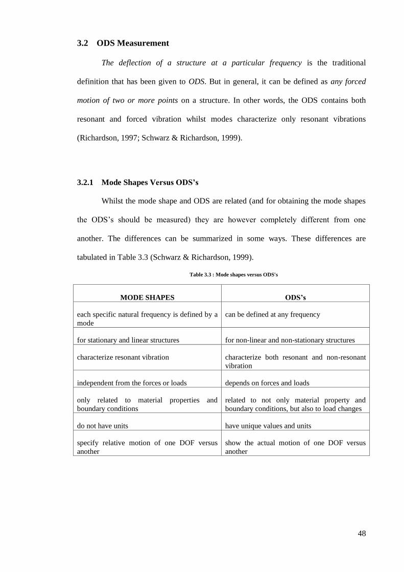
48

3.2 ODS Measurement

The deflection of a structure at a particular frequency is the traditional

definition that has been given to ODS. But in general, it can be defined as any forced

motion of two or more points on a structure. In other words, the ODS contains both

resonant and forced vibration whilst modes characterize only resonant vibrations

(Richardson, 1997; Schwarz & Richardson, 1999).

3.2.1 Mode Shapes Versus‎ODS’s

Whilst the mode shape and ODS are related (and for obtaining the mode shapes

the ODS’s should be measured) they are however completely different from one

another. The differences can be summarized in some ways. These differences are

tabulated in Table 3.3 (Schwarz & Richardson, 1999).

Table ‎3.3 : Mode shapes versus ODS's

MODE SHAPES ODS’s

each specific natural frequency is defined by a

mode

can be defined at any frequency

for stationary and linear structures for non-linear and non-stationary structures

characterize resonant vibration characterize both resonant and non-resonant

vibration

independent from the forces or loads depends on forces and loads

only related to material properties and

boundary conditions

related to not only material property and

boundary conditions, but also to load changes

do not have units have unique values and units

specify relative motion of one DOF versus

another

show the actual motion of one DOF versus

another

49

3.2.2 ODS Measurement

In both domains of time and frequency, the ODS can be obtained from any

forced motion. As was described for modal data collection, ODS data collection can be

made from a finite number of DOFs. Generally, it can be stated that “all experimental

modal parameters are obtained from measured ODS’s”. To put it in other words, post-

processing (curve fitting) a set of ODS data can result in obtaining the modal

parameters. In other words, within a frequency range, a set of FRFs and a set of ODS’s

could be similar. At or near a resonance peak, the ODS is dominated by a mode. As a

result, the ODS can be thought of as being just about equivalent to the mode shape

(Schwarz & Richardson, 1999).

Any ODS at each point is defined by magnitude and phase. To define a proper

ODS vector, at all response points, at least the relative magnitude and phase are

required. It denotes the fact that all the responses must be measured concurrently. This

situation will make the measurement difficult and expensive. A way to solve this

difficulty is via repeatable operation. This means that if the time waveform exactly

repeats in the sampling window, one set of data can be acquired every time. This

situation is also valid for steady state (stationary) operation situations that make using

ODS possible for many situations in industry (Schwarz & Richardson, 1999).

FRF data is derived from dividing the response by the excitation, and both the

magnitude and phase can be seen at each frequency. So, ODSs can be obtained from

FRF measurements. However, it becomes difficult when we learn that while measuring

the response, the excitation forces causing the response must be measured with it at the

same time. If not impossible, this would be tremendously tough. For this reason, ODS

data are obtained from Transmissibility measurements. When it is hard to measure the

excitation forces, transmissibility measurements are made. The measurement method is

similar to the way the FRF is measured, but instead of an excitation force, the response

50

is divided by a reference response signal. The units of the ODSs are response units per

unit of response at the reference DOF (Schwarz & Richardson, 1999).

Another way to obtain ODS measurements is ODS FRF, which is used when

excitation forces are immeasurable. In comparison to Transmissibility, the advantage of

ODS FRF is that the ODS FRF has peaks at resonances that make it easy to locate these

resonances. Like the Transmissibility, ODS FRF needs a reference response too

(Schwarz & Richardson, 1999).

3.3 Finite Element Modal Analysis

Finite Element Analysis (FEA) is a computational approach to solving

engineering problems by applying numerical methods. FEA has a vast number of

applications in the field of engineering such as stress analysis, heat transfer, fluid

mechanics, etc. The most important benefit of FEA is its ability to predict the real-world

behaviour of a structure or design concept. This leads to a considerable saving in both

time and investment. FEA in vibration analysis is known to be an analytical method to

determine the modal parameters of structures.

The main parameter in FEA is validation of the finite-element model because

finite-element models are rarely correct or accurate due to the many parameters that

create uncertainty in that model. Therefore, the results obtained from the FEA are

needed to be validated with measured test data, for example experimental modal

analysis data. So the test data themselves should have a high level of accuracy.

To validate a finite element modal analysis, corresponding natural frequency and

mode shapes are both needed. It should be mentioned that to compare parameters,

having corresponding amounts of natural frequencies is not enough. The mode shapes

should be compared too. This ensures a one-to-one correspondence between the

51

frequency and the mode shape. It should be noticed that a distinct mode shape is

associated with a distinct frequency (Schedlinski et al., 2004).

The finite-element model validation is accomplished through minimizing the

deviation between the identified and analytical eigenvalues and mode shapes. For this

purpose, it is assumed that the identified values are perfect and the whole error is from

the finite-element model. In the finite-element model, there are some parameters that

can be changed to decrease the deviation. These include geometry, element properties

(i.e. density, modules of elasticity, Poisson’s ratio, and the mesh size), and boundary

conditions.

Two methods were used in this research to compare the natural frequencies. The

first one is minimizing the error between the values obtained from FEA and EMA,

which should be less than 10%. The second one, as is shown in Figure 3.21 is to

compare the frequencies graphically through comparing the predicted and measured

results against each other. This method shows both the relative differences between the

frequencies as well as the global trends and advises possible reasons for these variances.

With a direct correlation between the values, the points will lie on a straight line with a

slope of 1.0 and if there is a random scatter, then an accurate representation of the

structure cannot be obtained using the finite-element model. This could be a

consequence of an inappropriate element type or a poor element mesh in the finite-

element model. It is also possible that there have been incorrect boundary conditions in

either the test or the analysis. If the points lie on a straight line, but with a slope other

than 1, then the problem may be a mass loading problem in the modal test or an

incorrect material property, such as elastic modulus or material density, in the finite-

element model (Agilent, 2008).

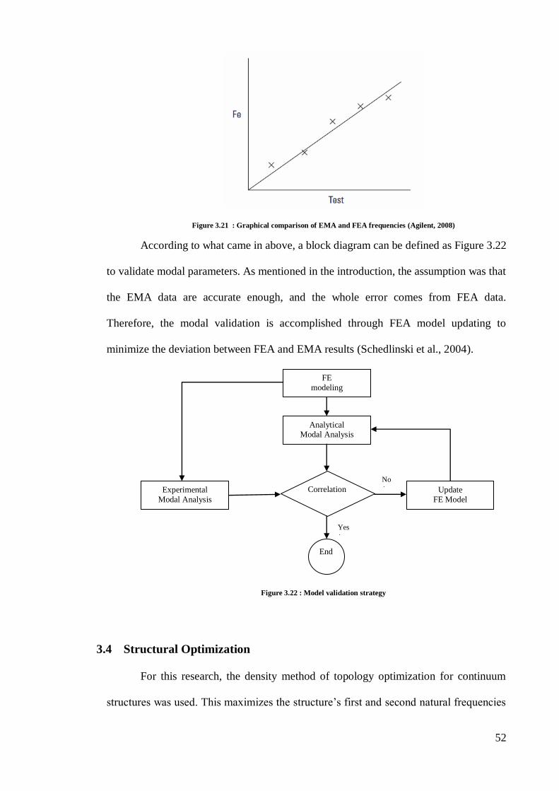
52

Figure ‎3.21 : Graphical comparison of EMA and FEA frequencies (Agilent, 2008)

According to what came in above, a block diagram can be defined as Figure 3.22

to validate modal parameters. As mentioned in the introduction, the assumption was that

the EMA data are accurate enough, and the whole error comes from FEA data.

Therefore, the modal validation is accomplished through FEA model updating to

minimize the deviation between FEA and EMA results (Schedlinski et al., 2004).

Figure ‎3.22 : Model validation strategy


For this research, the density method of topology optimization for continuum

structures was used. This maximizes the structure’s first and second natural frequencies

FE

modeling

Analytical Modal Analysis

Experimental

Modal Analysis

Correlation Update

FE Model

End

No

Yes

53

out of excitation frequency range with respect to the manufacturability of the new

structure.

Continuum topology optimization seeks to determine the inner holes and also

the internal and external boundaries. One of the methodologies used in continuum

topology optimization is the density method. Each element should be solid or void

meaning its density should take an amount of 1 or 0 or a value in between. The density

of an element can be presented as:

(3.2)

Where the (1-a) (1-b) represents the total volume of void in an element. As can

be seen here, a=b=0 presents total void and a=b=1 presents solid element and the void

size variables varying between 0 and 1 (Rosen, 1961).

The optimization in this research has been done using Altair-Hyper Works

software. It is a finite-element based structural analysis and optimization software. This

software is a response-based optimization tool. Responses are defined as quantities in

the analysis which can be constrained or optimized. The aim of this research is to

maximize the natural frequencies of the structure according to manufacturability of the

new structure. Therefore, the objective function is assumed as frequency that should be

optimized (maximized) and the constraint assumed as volume-fraction.

Altair-Hyper Works solves the optimization problems by either Homogenization

or density method. The density method is the default method however. The main

parameters in optimization problems that need to be solved are Objective, Constraints,

and Design Variables. Objective function and constraint function are structural

responses obtained from a finite-element analysis. Design variables depend on the type

of optimization (Rosen, 1961).

The software uses an iterative solution. In the first step, the physical problem

will be analysed, and then a convergence test is carried out. After that the design

54

sensitivity analysis is performed, and an approximate optimization solution is presented

based on the sensitivity information. Finally, based on the postulation that only minor

variations occur in the design with each optimization step, the steps will be repeated

again. Furthermore, in this software, three types of elements are available; solid

elements, shell elements, and 1-D elements. In the density method, each element has a

variable that presents the material density. For this research, a solid element has been

used to perform the optimization and modal analysis (Rosen, 1961).

As it turned out, the constraint in this research is manufacturability of the new

structure. In this work, the assumption is that the structure should be reinforced by

adding simple new parts to the structure rather than remanufacturing the structure.

However, the problem is that software can only give a visual estimation of density

variety for designable area and not an exact solution. Thus, the model should be defined

in such a way that the best post processing can be realized. It is also assumed that the

simplest form of optimization is needed because usually, the results from the software

have complicated forms.

55

Chapter four

4 Results

In this chapter, the results obtained or calculated from different sections of this

research are presented in the form of the text, tables and figures. In the first section, the

results obtained from the Modal Testing and ODS analysis are presented. In the next

section, the validated finite-element model and the validation methods are shown.

Finally, the two different optimized models obtained from the Altair-Hyper Works

software are presented.

4.1 Experimental Modal Analysis

In this section the results extracted from MEScope VES software for the Modal

Testing is presented. Modal Testing consists of three main steps, i.e. modelling the

geometry of the structure, setting up the system, acquire FRF data using FRF-analyser

VI, and post processing the results (Chiat, 2008). Each step is described below, and the

setting for each step and sub-step is detailed.

Step 1: Modelling the Geometry of the Structure

In this step, the measurement response points and the impact point were chosen.

Numbered stickers were used to locate the point numbers. In total 72 measurement

points were located on the structure. The structure was then modelled in MEscope VES

according to its real dimensions and the measurement points and global coordinates

defined in the MEscope VES software. The model is shown in Figure 4.1.

56

Figure ‎4.1 : MEscope VES model of the structure

Step 2: Setting up the system and acquiring FRF data with FRF-analyser

VI (LabVIEW software Virtual Instrument)

In this step, the FRF data should be obtained and be saved using measured

impact force and responses via the FRF analyser VI.

Before starting to obtain the data, the accelerometer needs to be calibrated. For

this purpose, the accelerometer is connected to a calibrator which vibrates with an

acceleration magnitude of RMS value 10m/S2

at a frequency of 159.2 Hz. Furthermore,

the accelerometer 3rd axis cable is connected to one of the channels of the 4-channel

data acquisition hardware. This is connected to the laptop containing the LabVIEW

software. The sensitivity calculated for this axis was 9.8 mV/g which is close the value

printed on the case of the accelerometer; 9.9mV/g. Therefore, the other sensitivities for

other axis are assumed to be correct. The accelerometer calibration needs to be done

only once during the EMA.

57

Furthermore, the initial settings of the block diagram were configured as:

sampling frequency=2000 Hz, number of samples of DAQ=14000, threshold value=1.0,

number of samples of trigger=10000, number of averages=5. The windowing options

were set to “Rectangular” for input and “Exponential” for the output response. These

options also only need be configured once during the EMA.

The next step follows what introduced in the operation’s flow chart for the FRF-

analyzer VI as depicted in Figure 3.8. The accelerometer is attached to a mesurement

point. The front pannel of the FRF-analyzer VI is set and the program is executed. The

structure is excited at a fixed impact point by the impact hammer andthe time domain

impulsive force is checkedto prevent double knocking.The results are then saved and

the process is iterated acording to the flowchart. The measurment were done for 72

points in three x, y and z directions. This resulted in 216 FRF measurements.

Step 3: Post processing the results

This step consists of importing the FRFs to MEscope VES software to determine

the natural frequencies of the structure and animate the mode shapes corresponding to

specific natural frequencies. The FRFs are imported to the software and assigned to the

measurement points of the structure. The natural frequencies and mode shapes

according to these natural frequencies are then obtained by performing curve fitting on

the imaginary part of the FRFs. The frequency range for this analysis was set between

10 Hz and 70 Hz. It was set from 10 Hz to prevent the effects of rigid body modes on

the flexible modes in the curve fitting results. The overlay FRFs for the frequency range

between 0 Hz and 70 Hz is shown in Figure 4.2 to indicate the influence of the rigid

body mode FRFs. After neglecting the rigid body modes, the resulted FRF between 10

Hz and 70 Hz is shown in Figure 4.3. Also, the curve fitting results are depicted in

Figure 4.4.

58

Figure ‎4.2 : Overlay FRFs between 0 and 70 Hz to indicate the rigid body modes

Figure ‎4.3 : Overlay FRFs between 10Hz and 70Hz

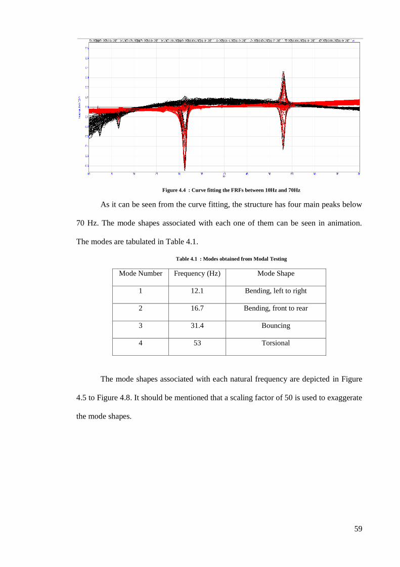
59

Figure ‎4.4 : Curve fitting the FRFs between 10Hz and 70Hz

As it can be seen from the curve fitting, the structure has four main peaks below

70 Hz. The mode shapes associated with each one of them can be seen in animation.

The modes are tabulated in Table 4.1.

Table ‎4.1 : Modes obtained from Modal Testing

Mode Number Frequency (Hz) Mode Shape

1 12.1 Bending, left to right

2 16.7 Bending, front to rear

3 31.4 Bouncing

4 53 Torsional

The mode shapes associated with each natural frequency are depicted in Figure

4.5 to Figure 4.8. It should be mentioned that a scaling factor of 50 is used to exaggerate

the mode shapes.

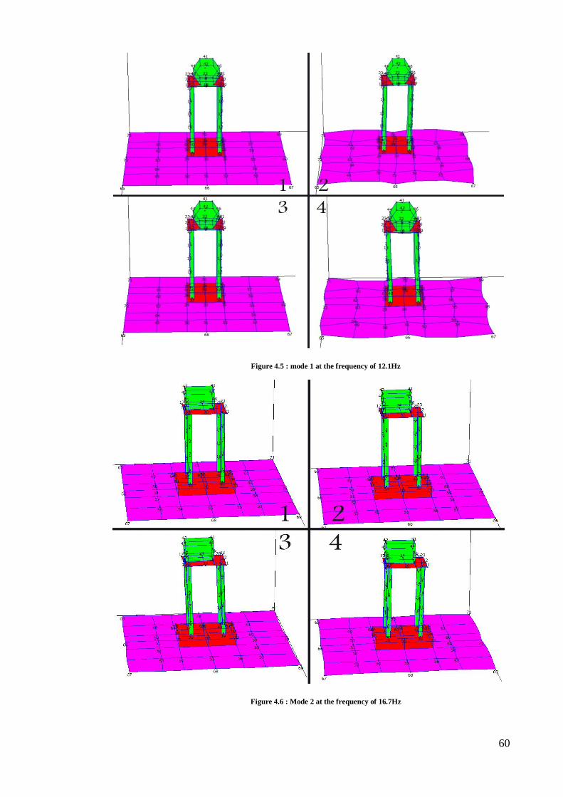
60

Figure ‎4.5 : mode 1 at the frequency of 12.1Hz

Figure ‎4.6 : Mode 2 at the frequency of 16.7Hz

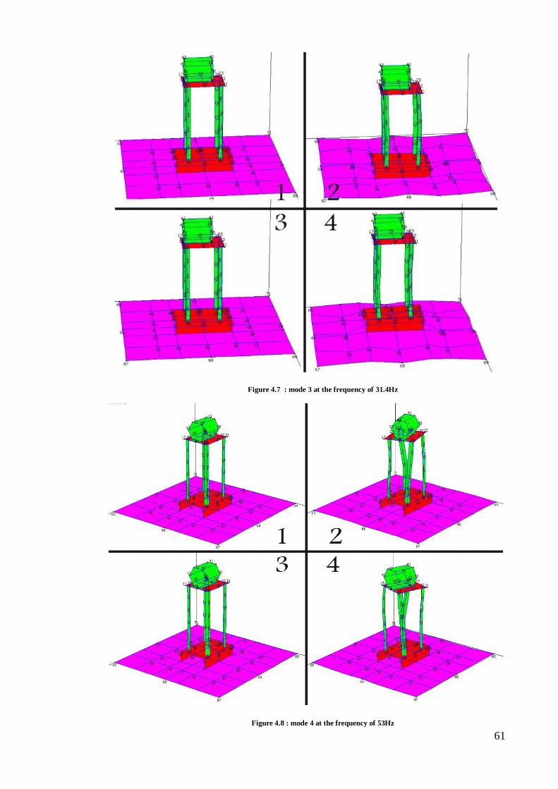
61

Figure ‎4.7 : mode 3 at the frequency of 31.4Hz

Figure ‎4.8 : mode 4 at the frequency of 53Hz

62

4.2 ODS Measurement

The set up for the ODS measurement is almost the same as the Modal Testing.

However, instead of using an impact hammer to excite the structure, the time domain

data are collected during the operation of the motor in specific frequencies. For this

research, the ODS measurement has been done for two frequencies, namely, 12.1 Hz

and 16 Hz. The main reason that these two frequencies were chosen was the fact that

based on the Modal Testing results, there are two modes below 20 Hz at 12.1 Hz and 16

Hz. The three main steps of EMA are described below and the results are presented for

the two frequencies separately.

Step 1: Modelling the geometry of the structure

This step is completely the same as what was described in section 4.1.1.

Step 2: Setting up the system and acquire FRF data via FRF-analyser VI

In this step, the FRF data should be obtained and be saved using measured

impact force and responses via the FRF analyser VI.

The VI used for ODS measurement is similar to the one used for Modal Testing

(Chiat, 2008). The initial settings of the block diagram were configured as follows:

sampling frequency=2000 Hz, number of samples of DAQ=14000, threshold value=0,

number of samples of trigger=10000, number of averages=5. The windowing options

were set to “Hanning” for both input and output signals.

Performing ODS measurement is similar to Modal Testing but instead of the

impact hammer, a uniaxial accelerometer is used as the reference point. The tri-axial

accelerometer is roving and by following the flowchart as depicted in Figure 4.9, the

FRF data was collected and saved for 72 points in three x, y and z directions.This

resulted in 216 FRF measurements.

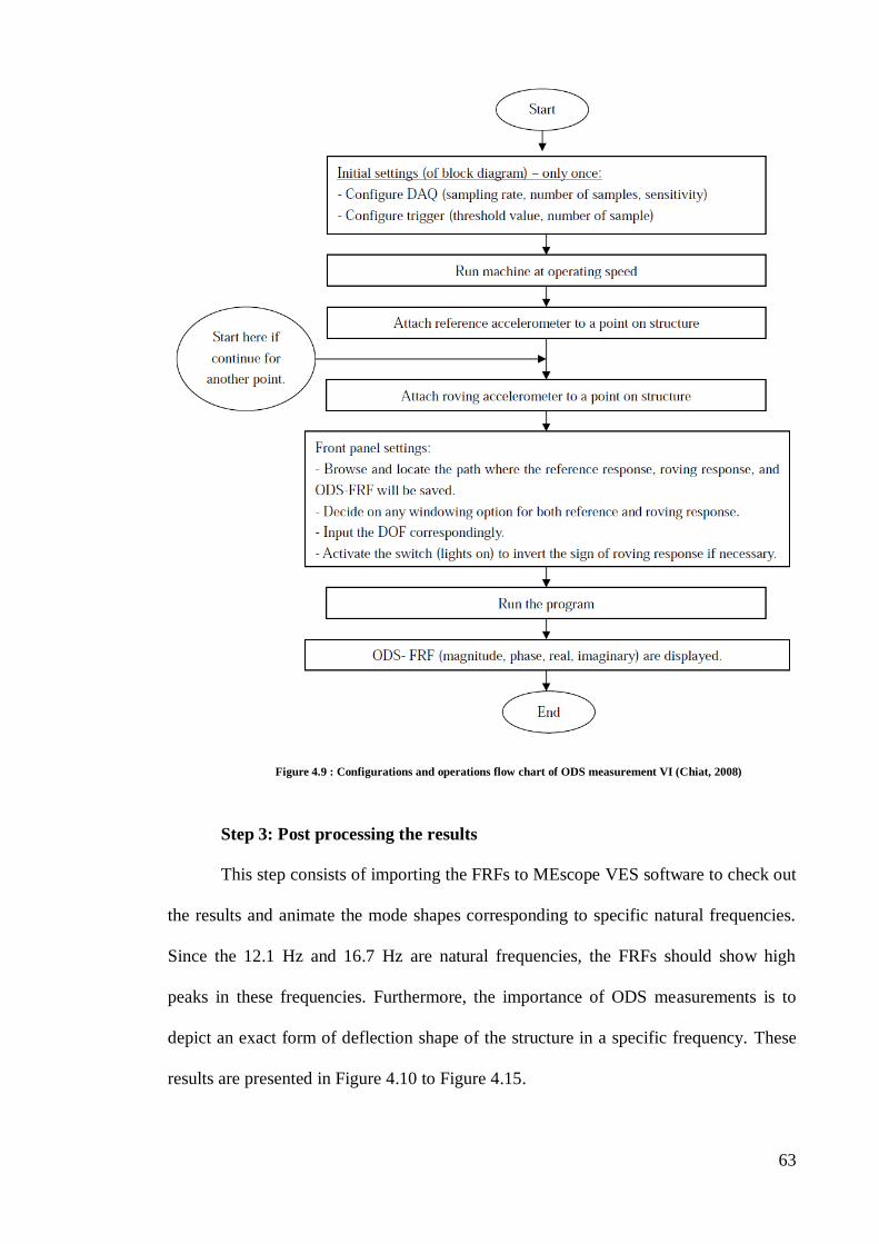
63

Figure ‎4.9 : Configurations and operations flow chart of ODS measurement VI (Chiat, 2008)

Step 3: Post processing the results

This step consists of importing the FRFs to MEscope VES software to check out

the results and animate the mode shapes corresponding to specific natural frequencies.

Since the 12.1 Hz and 16.7 Hz are natural frequencies, the FRFs should show high

peaks in these frequencies. Furthermore, the importance of ODS measurements is to

depict an exact form of deflection shape of the structure in a specific frequency. These

results are presented in Figure 4.10 to Figure 4.15.

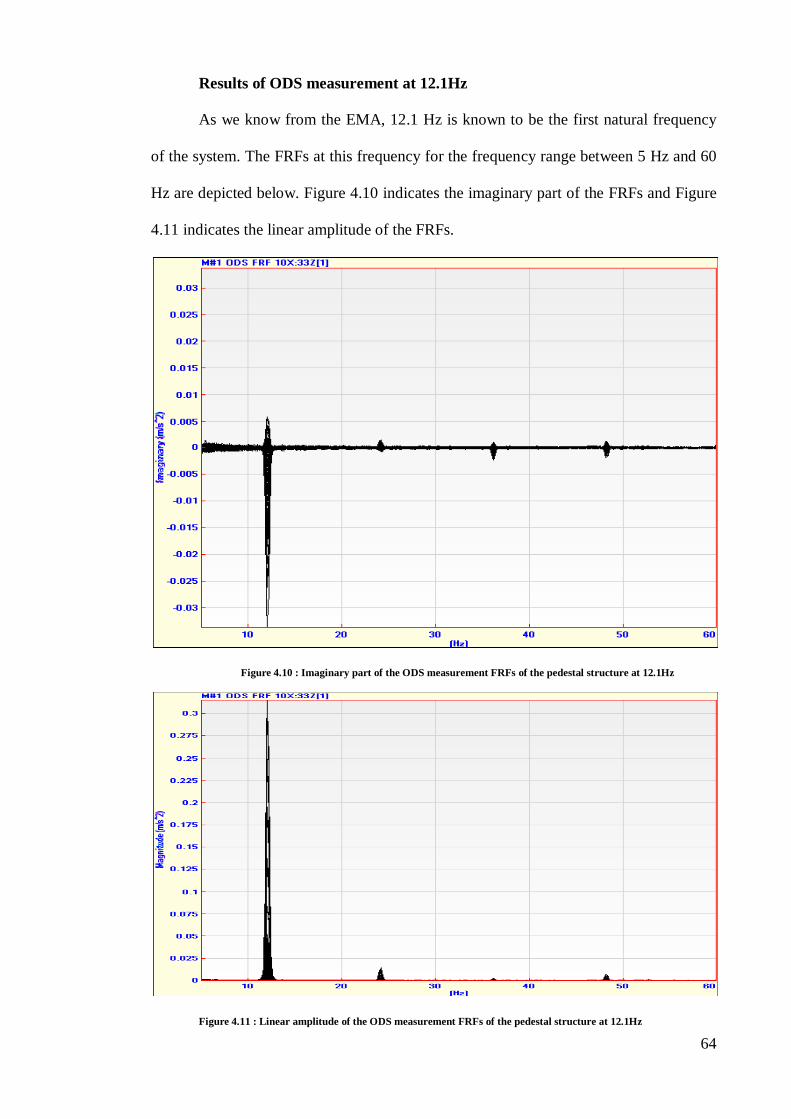
64

Results of ODS measurement at 12.1Hz

As we know from the EMA, 12.1 Hz is known to be the first natural frequency

of the system. The FRFs at this frequency for the frequency range between 5 Hz and 60

Hz are depicted below. Figure 4.10 indicates the imaginary part of the FRFs and Figure

4.11 indicates the linear amplitude of the FRFs.

Figure ‎4.10 : Imaginary part of the ODS measurement FRFs of the pedestal structure at 12.1Hz

Figure ‎4.11 : Linear amplitude of the ODS measurement FRFs of the pedestal structure at 12.1Hz

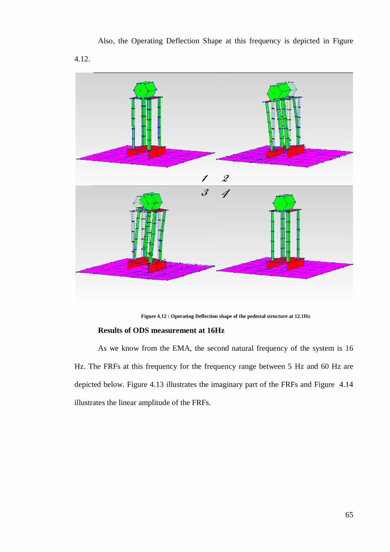
65

Also, the Operating Deflection Shape at this frequency is depicted in Figure

4.12.

Figure ‎4.12 : Operating Deflection shape of the pedestal structure at 12.1Hz

Results of ODS measurement at 16Hz

As we know from the EMA, the second natural frequency of the system is 16

Hz. The FRFs at this frequency for the frequency range between 5 Hz and 60 Hz are

depicted below. Figure 4.13 illustrates the imaginary part of the FRFs and Figure 4.14

illustrates the linear amplitude of the FRFs.

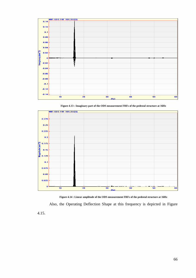
66

Figure ‎4.13 : Imaginary part of the ODS measurement FRFs of the pedestal structure at 16Hz

Figure ‎4.14 : Linear amplitude of the ODS measurement FRFs of the pedestal structure at 16Hz

Also, the Operating Deflection Shape at this frequency is depicted in Figure

4.15.

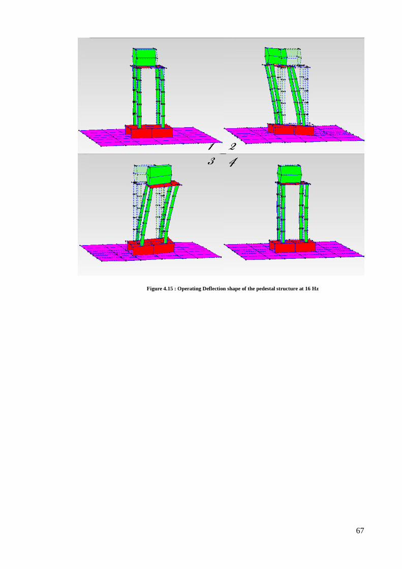
67

Figure ‎4.15 : Operating Deflection shape of the pedestal structure at 16 Hz

68


As mentioned in the methodology, the main parameter in FEA is the validation

of the model. For this research, the geometry of the structure was first modelled using

SolidWorks software. This model was exported to Altair Hyper Works and the Modal

analysis was performed on it. Then, according to methods introduced in the

methodology, the FEA model was validated in comparison to EMA results. These two

phases are described below.

4.3.1 Geometry Design and Performing Modal Analysis

For this section of work, the geometry was modelled in SolidWorks according to

the exact dimensions of the real structure. To simplify the model, some details such as

washers, nuts, bolts and welding are neglected without significant loss in accuracy.

Furthermore, for simplicity, the motor was designed in a way that its density is equal to

the other parts of the structure. The designed geometry is shown in Figure 4.16 and

Figure 4.17.

Figure ‎4.16 : Designed model by SolidWorks – isometric view

69

Figure ‎4.17 : Designed model by SolidWorks

In the next step, this geometry was exported to the Altair Hyper Works software

as an *.igs file. The model was then meshed with a fixed element size of 15 mm and a

minimum of 3 mm for “Proximity”. The element type is the 3D tetra-mesh for solid

volumes. This model is depicted in Figure 4.18.

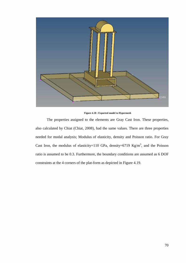
70

Figure ‎4.18 : Exported model to Hypermesh

The properties assigned to the elements are Gray Cast Iron. These properties,

also calculated by Chiat (Chiat, 2008), had the same values. There are three properties

needed for modal analysis; Modulus of elasticity, density and Poisson ratio. For Gray

Cast Iron, the modulus of elasticity=110 GPa, density=6719 Kg/m3, and the Poisson

ratio is assumed to be 0.3. Furthermore, the boundary conditions are assumed as 6 DOF

constraints at the 4 corners of the plat-form as depicted in Figure 4.19.

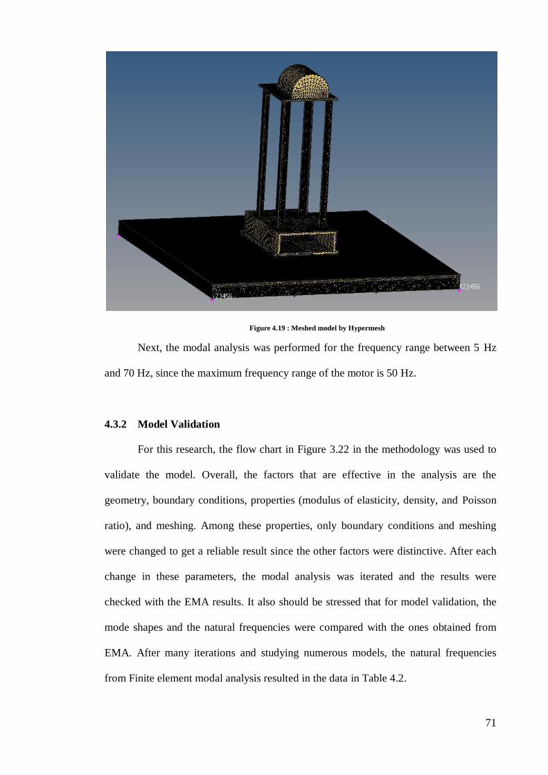
71

Figure ‎4.19 : Meshed model by Hypermesh

Next, the modal analysis was performed for the frequency range between 5 Hz

and 70 Hz, since the maximum frequency range of the motor is 50 Hz.

4.3.2 Model Validation

For this research, the flow chart in Figure 3.22 in the methodology was used to

validate the model. Overall, the factors that are effective in the analysis are the

geometry, boundary conditions, properties (modulus of elasticity, density, and Poisson

ratio), and meshing. Among these properties, only boundary conditions and meshing

were changed to get a reliable result since the other factors were distinctive. After each

change in these parameters, the modal analysis was iterated and the results were

checked with the EMA results. It also should be stressed that for model validation, the

mode shapes and the natural frequencies were compared with the ones obtained from

EMA. After many iterations and studying numerous models, the natural frequencies

from Finite element modal analysis resulted in the data in Table 4.2.

72

Table ‎4.2 : Modal parameter resulted from finite element modal analysis

Mode number Natural frequency (Hz) Mode shape

1 13.2 Bending- left to right

2 17.9 Bending- front to rear

3 28.1 Bouncing

4 58 Torsional

The analytical mode shapes are depicted in Figure 4.20 to Figure 4.23.

Figure ‎4.20 : Anlytical mode shape- mode1- 13.2 Hz

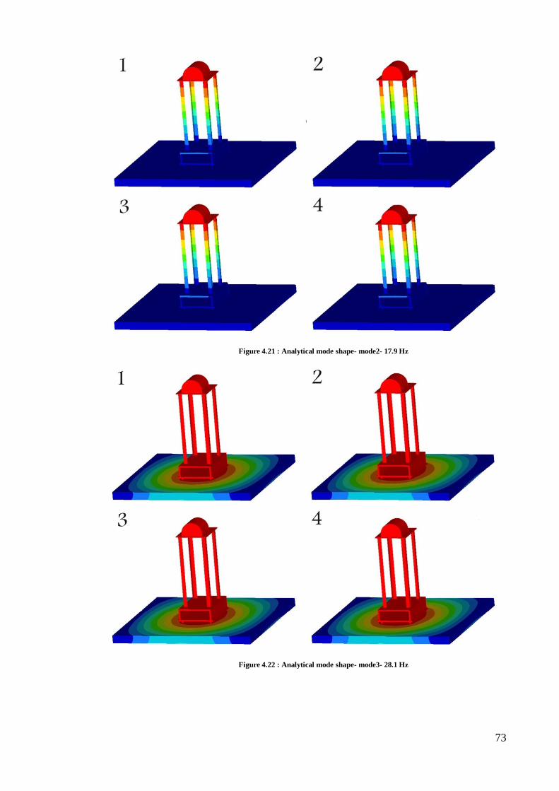
73

Figure ‎4.21 : Analytical mode shape- mode2- 17.9 Hz

Figure ‎4.22 : Analytical mode shape- mode3- 28.1 Hz

74

Figure ‎4.23 : Analytical mode shape- mode4- 58 Hz

4.4 Optimization

As was the case earlier, the optimization of the structure was done to maximize

the first and second natural frequencies to allow manufacturability of the new structure.

In this way, the operator will be able to optimize the structure by adding simple new

parts to the structure and reinforcing it rather than rebuilding the structure.

For this purpose, several responses (objective functions and constraints of

optimization) were defined to the Hypermesh. Based on the visual estimation

subsequently obtained from the software, a new model of the structure was developed.

Modal analysis was then performed on this new model and the results of different

assumed models were compared to choose the best one.

Furthermore, the designable area for this work assumed two parts consisting of

the pedestal and the platform. The reason is that the movement of the structure in

resonances comes not only from the pedestal but the platform also shows deformation.

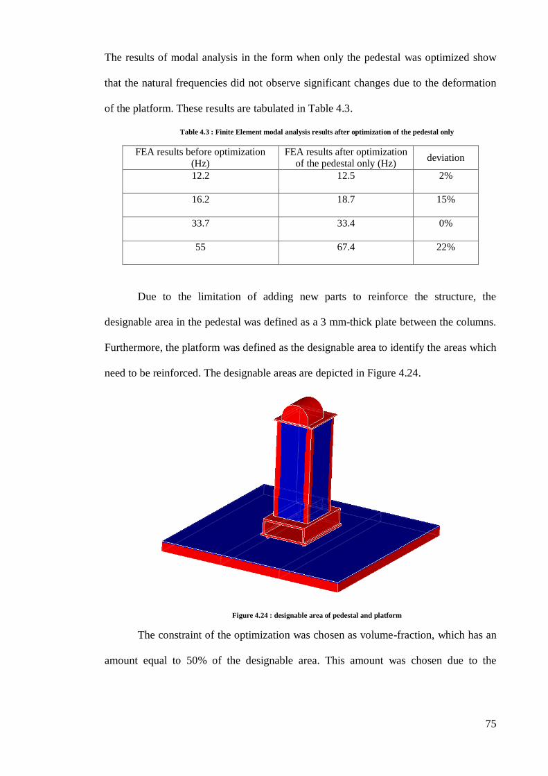
75

The results of modal analysis in the form when only the pedestal was optimized show

that the natural frequencies did not observe significant changes due to the deformation

of the platform. These results are tabulated in Table 4.3.

Table ‎4.3 : Finite Element modal analysis results after optimization of the pedestal only

FEA results before optimization

(Hz)

FEA results after optimization

of the pedestal only (Hz) deviation

12.2 12.5 2%

16.2 18.7 15%

33.7 33.4 0%

55 67.4 22%

Due to the limitation of adding new parts to reinforce the structure, the

designable area in the pedestal was defined as a 3 mm-thick plate between the columns.

Furthermore, the platform was defined as the designable area to identify the areas which

need to be reinforced. The designable areas are depicted in Figure 4.24.

Figure ‎4.24 : designable area of pedestal and platform

The constraint of the optimization was chosen as volume-fraction, which has an

amount equal to 50% of the designable area. This amount was chosen due to the

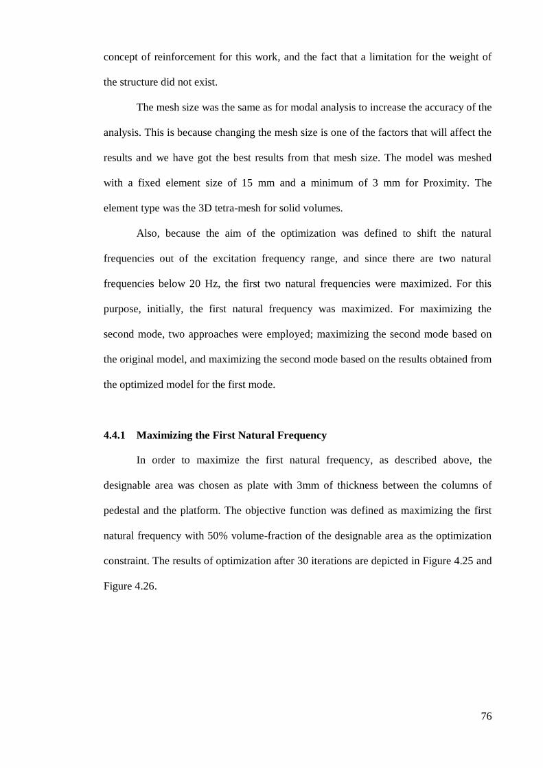
76

concept of reinforcement for this work, and the fact that a limitation for the weight of

the structure did not exist.

The mesh size was the same as for modal analysis to increase the accuracy of the

analysis. This is because changing the mesh size is one of the factors that will affect the

results and we have got the best results from that mesh size. The model was meshed

with a fixed element size of 15 mm and a minimum of 3 mm for Proximity. The

element type was the 3D tetra-mesh for solid volumes.

Also, because the aim of the optimization was defined to shift the natural

frequencies out of the excitation frequency range, and since there are two natural

frequencies below 20 Hz, the first two natural frequencies were maximized. For this

purpose, initially, the first natural frequency was maximized. For maximizing the

second mode, two approaches were employed; maximizing the second mode based on

the original model, and maximizing the second mode based on the results obtained from

the optimized model for the first mode.

4.4.1 Maximizing the First Natural Frequency

In order to maximize the first natural frequency, as described above, the

designable area was chosen as plate with 3mm of thickness between the columns of

pedestal and the platform. The objective function was defined as maximizing the first

natural frequency with 50% volume-fraction of the designable area as the optimization

constraint. The results of optimization after 30 iterations are depicted in Figure 4.25 and

Figure 4.26.

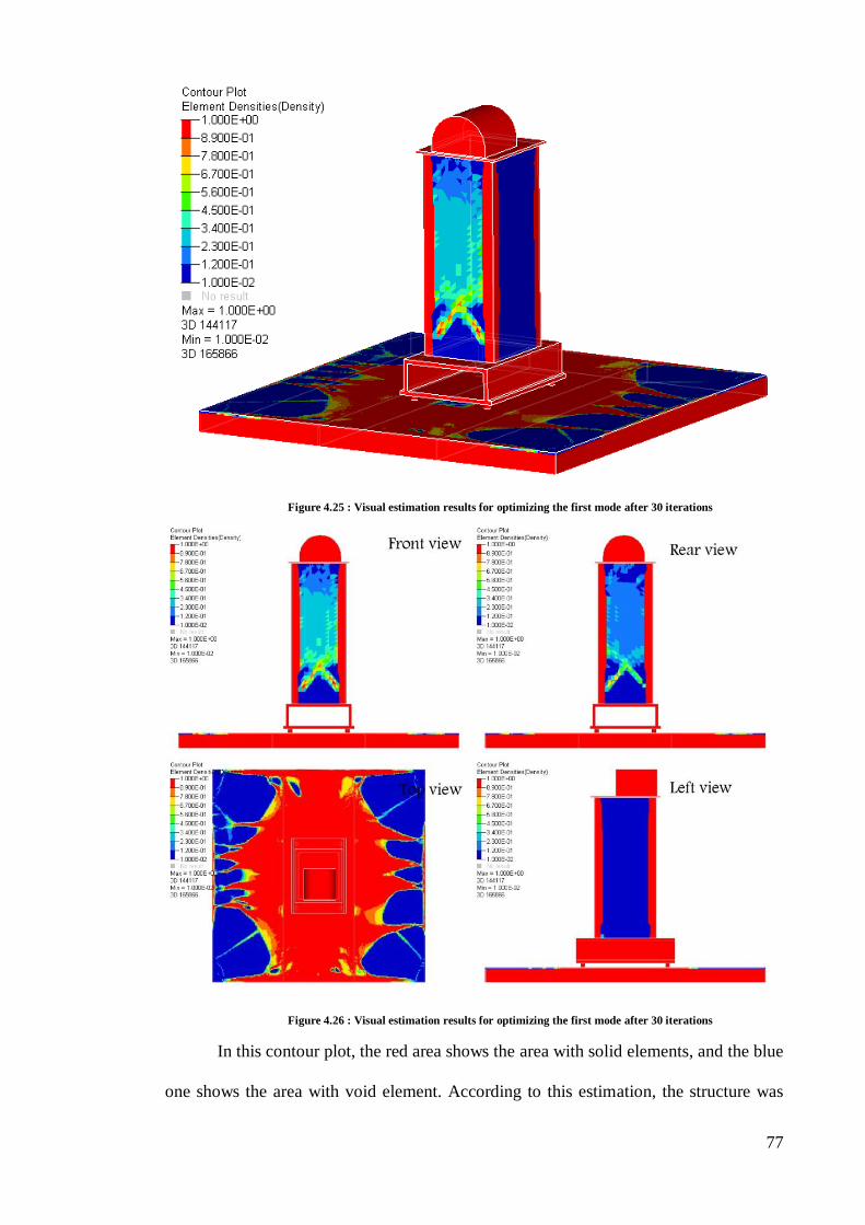
77

Figure ‎4.25 : Visual estimation results for optimizing the first mode after 30 iterations

Figure ‎4.26 : Visual estimation results for optimizing the first mode after 30 iterations

In this contour plot, the red area shows the area with solid elements, and the blue

one shows the area with void element. According to this estimation, the structure was

78

reinforced in both the platform and the pedestal. The pedestal was reinforced by adding

two cross-plates, and the platform was reinforced by adding two vertical plates.

Optimized structure is depicted in Figure 4.27 and Figure 4.28. The mode shapes and

the natural frequencies for the optimized structure are tabulated in Table 4.4.

Figure ‎4.27 : Optimized design structure according to visual estimations for the first mode

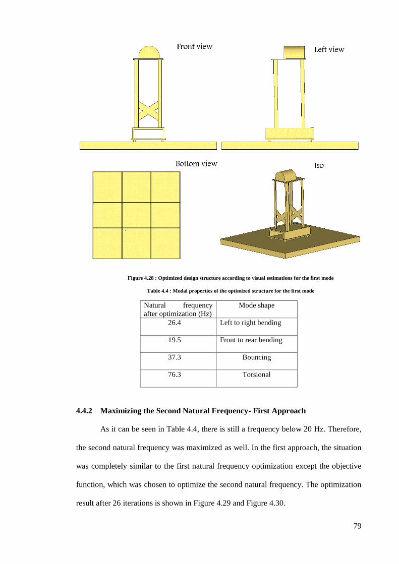
79

Figure ‎4.28 : Optimized design structure according to visual estimations for the first mode

Table ‎4.4 : Modal properties of the optimized structure for the first mode

Natural frequency

after optimization (Hz)

Mode shape

26.4 Left to right bending

19.5 Front to rear bending

37.3 Bouncing

76.3 Torsional

4.4.2 Maximizing the Second Natural Frequency- First Approach

As it can be seen in Table 4.4, there is still a frequency below 20 Hz. Therefore,

the second natural frequency was maximized as well. In the first approach, the situation

was completely similar to the first natural frequency optimization except the objective

function, which was chosen to optimize the second natural frequency. The optimization

result after 26 iterations is shown in Figure 4.29 and Figure 4.30.

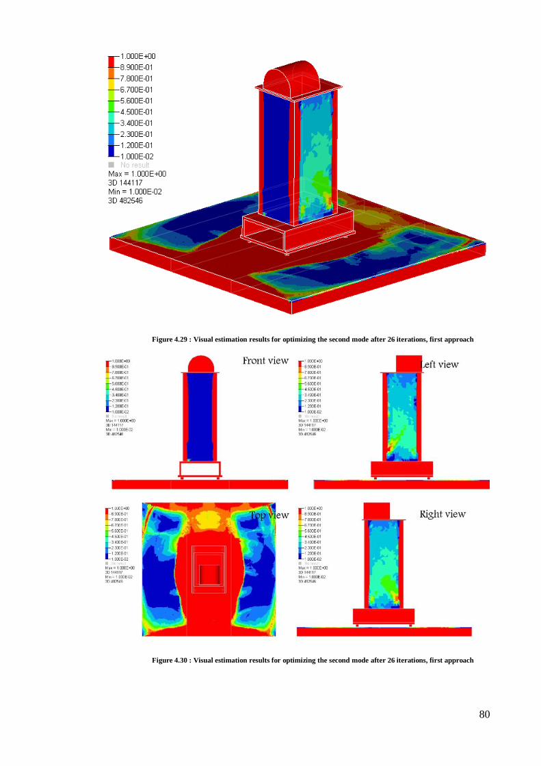
80

Figure ‎4.29 : Visual estimation results for optimizing the second mode after 26 iterations, first approach

Figure ‎4.30 : Visual estimation results for optimizing the second mode after 26 iterations, first approach

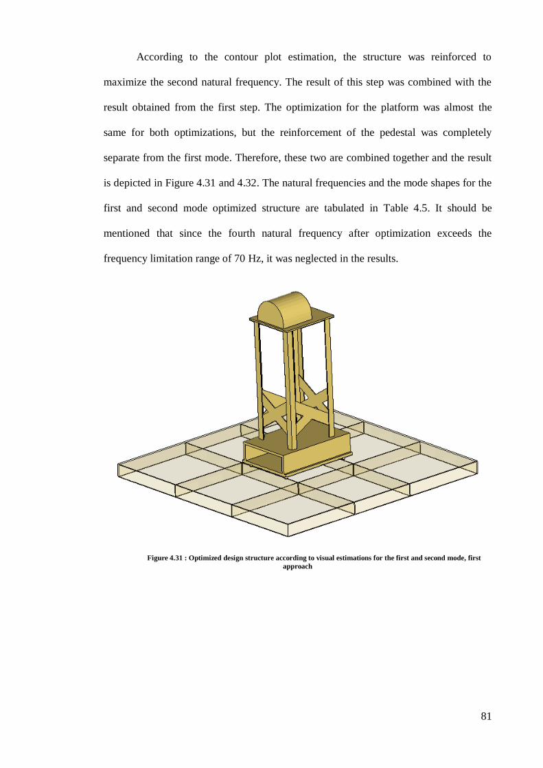
81

According to the contour plot estimation, the structure was reinforced to

maximize the second natural frequency. The result of this step was combined with the

result obtained from the first step. The optimization for the platform was almost the

same for both optimizations, but the reinforcement of the pedestal was completely

separate from the first mode. Therefore, these two are combined together and the result

is depicted in Figure 4.31 and 4.32. The natural frequencies and the mode shapes for the

first and second mode optimized structure are tabulated in Table 4.5. It should be

mentioned that since the fourth natural frequency after optimization exceeds the

frequency limitation range of 70 Hz, it was neglected in the results.

Figure ‎4.31 : Optimized design structure according to visual estimations for the first and second mode, first

approach

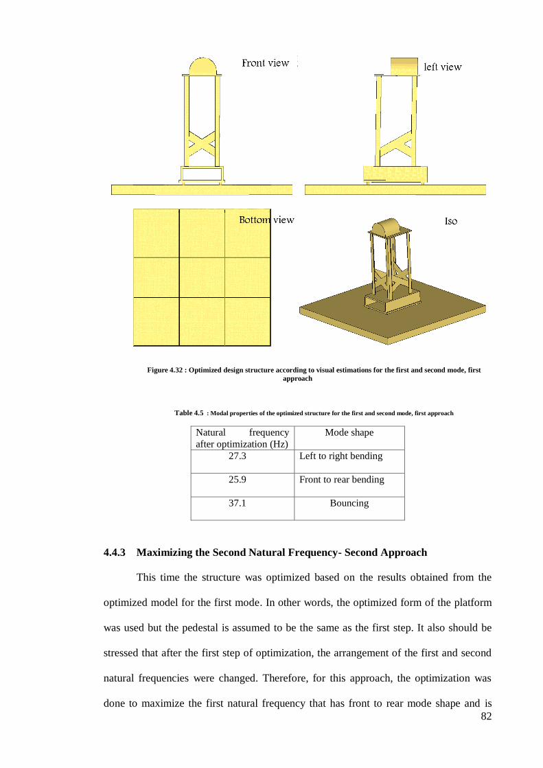
82

Figure ‎4.32 : Optimized design structure according to visual estimations for the first and second mode, first

approach

Table ‎4.5 : Modal properties of the optimized structure for the first and second mode, first approach

Natural frequency


Mode shape



37.1 Bouncing

4.4.3 Maximizing the Second Natural Frequency- Second Approach

This time the structure was optimized based on the results obtained from the

optimized model for the first mode. In other words, the optimized form of the platform

was used but the pedestal is assumed to be the same as the first step. It also should be

stressed that after the first step of optimization, the arrangement of the first and second

natural frequencies were changed. Therefore, for this approach, the optimization was

done to maximize the first natural frequency that has front to rear mode shape and is

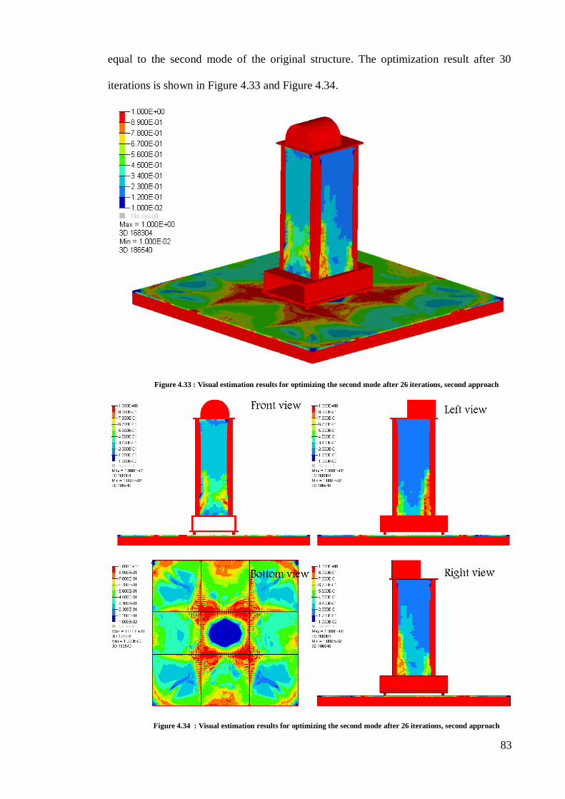
83

equal to the second mode of the original structure. The optimization result after 30

iterations is shown in Figure 4.33 and Figure 4.34.

Figure ‎4.33 : Visual estimation results for optimizing the second mode after 26 iterations, second approach

Figure ‎4.34 : Visual estimation results for optimizing the second mode after 26 iterations, second approach

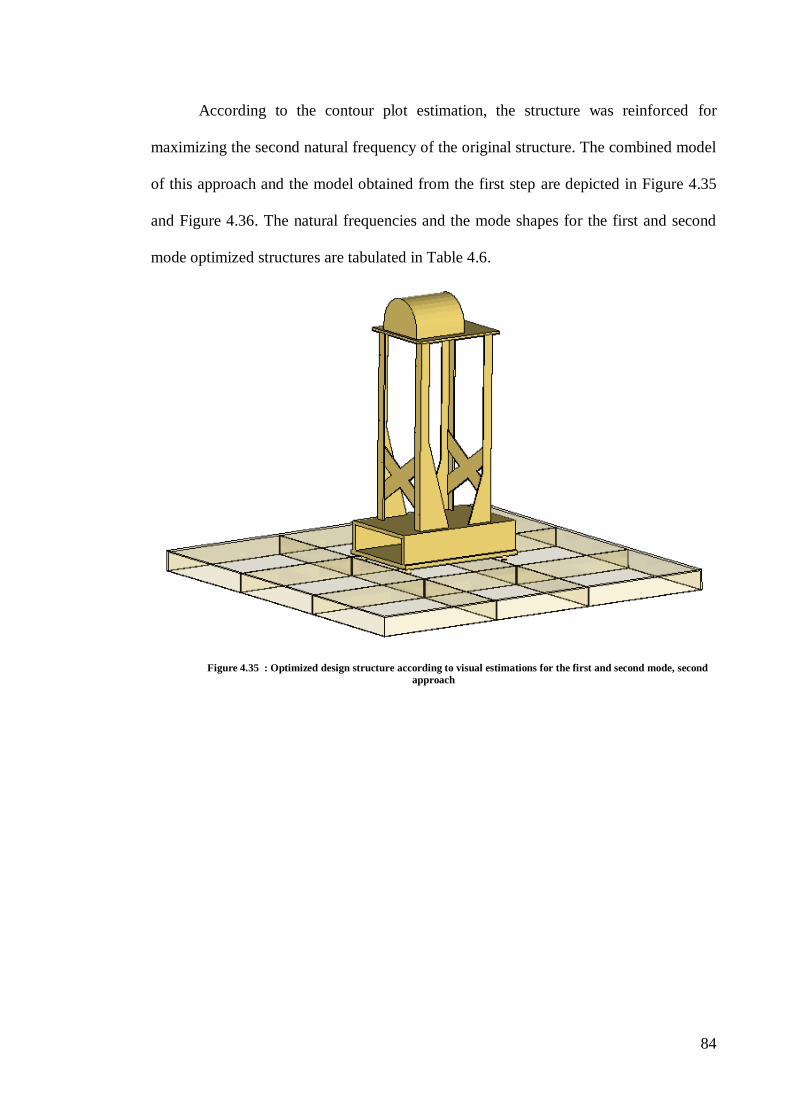
84

According to the contour plot estimation, the structure was reinforced for

maximizing the second natural frequency of the original structure. The combined model

of this approach and the model obtained from the first step are depicted in Figure 4.35

and Figure 4.36. The natural frequencies and the mode shapes for the first and second

mode optimized structures are tabulated in Table 4.6.

Figure ‎4.35 : Optimized design structure according to visual estimations for the first and second mode, second

approach

85

Figure ‎4.36 : Optimized design structure according to visual estimations for the first and second mode, second

approach

Table ‎4.6 : Modal properties of the optimized structure for the first and second mode, second approach

Natural frequency


Mode shape



37.2 Bouncing

86

Chapter Five

5 Discussion

This chapter discusses the results obtained from the different parts of this

research presented in pervious chapter. It contains four subchapters; Experimental

modal analysis, ODS measurement, Finite element modal analysis, and structural

optimization.

5.1 Experimental Modal Analysis

Every vibration analysis needs experimental data to describe dynamic properties

of the system. As it has been mentioned earlier, these experimental data can be obtained

by collecting modal data (modal testing) or by collecting operating data (ODS). But it is

always difficult to distinguish the preferred one. To optimize the system, we needed the

modal data since it is only the modal data that gives true principle characteristics of the

system. On the other hand, the optimization was supposed to be performed in order to

decrease vibration failures of the system due to the motor operating effects. Hence, we

needed the force response of the system that only the ODS measurement can provide

such information, because the modal data are independent of the forces on the system.

Furthermore, only ODS can depict how the structure behaves in service. It is very

important for optimization of the system because it can present an initial estimation

which shows the parts of the structure that is needed to be reinforced. As it came in the

results, both the Modal testing and the ODS measurement have been carried out for this

research as discussed below.

87

5.1.1 Modal Testing

The aim of this research is to optimize the structure for the occasions that the

motor operates below 50 Hz. Therefore, it is important to identify the modes below 50

Hz. For this purpose, the Modal testing has been performed on the structure and as the

results show, this structure has 4 modes below this frequency. Such data are the most

basic data that are used to validate the FEA model and after the optimization, the results

compared with the pervious data have been already done on this structure by (Chiat,

2008). The results are compared in Table 5.1.

Table ‎5.1 : Comparison of obtained modal parameters with results from (Chiat, 2008)

EMA results

from (Chiat,

2008) (Hz)

EMA results from my

experience (Hz) Mode Shape Error

12 12.1 Left-right bending 0.8%

16 16.7 Front-rear bending 4.4%

31.4 31.4 Bouncing 0%

47.1 53 Torsional 12.5%

The maximum operating frequency of the motor is 50Hz but the using frequency

range of the motor will be at most 20 Hz. obviously, the structure has two modes in the

low frequency, below 20 Hz, that can cause resonant vibration and make the structure

unstable. The first mode occurs at 12.1 Hz and is a left-right bending mode. The second

mode occurs at 16.7 Hz and is a rear-front bending mode. Furthermore, from the results

obtained from MEscope, it can be observed that these two modes lead to deformation

not only in the pedestal, but also a deformation in the platform. It is important because

to optimize the structure we needed to know what parts of the structure should be

selected as the designable area. Otherwise, the optimization will not be reliable.

On the other hand, optimization of the structure was going to perform by FEA

based software. Therefore, an exact Finite-Element model was vital for this research.

88

The finite element model is not reliable on its own and needs to be validated by

experimental data. Hence, the experimental modal parameters were used to validate the

Finite Element model.

5.2 ODS Measurement

As it has already been mentioned, recognizing the natural frequencies is crucial

to optimize the structure. However, along with reorganization of the natural frequencies

and the mode shapes, the real deflection of the structure is also quite important that has

been done by performing the ODS measurement. Similarly, the results of the ODS can

validate the Modal Testing data. Therefore, the ODS measurement has been done for

two natural frequencies at 12.1 Hz and 16 Hz.

As it has been mentioned in the methodology, the deflection shape resulted from

ODS measurement at the natural frequencies should be similar to the mode shapes of

the structure. The animation results of the ODS measurements show that the deflection

shape of the structure at 12.1 Hz is a combination of both left-right bending and rear-

front bending whose major part is left-right bending. This is very close to the mode

shape of the structure at 12.1 Hz. Furthermore, FRFs show a high peak at 12.1 Hz that

validate the existence of a natural frequency at this frequency. The results at the 16 Hz

are as well as 12.1 Hz. The major part of the deflection shape at 16 Hz is rear-front

bending that is similar to the second mode shape of the structure. Furthermore, the FRFs

show a high peak at 16 Hz that validate existence of a mode at this frequency.

The EMA data show that there are two modes that need to be maximized out of

the using frequency range of the motor. Furthermore, these results illustrate that the two

parts of the structure have the most deformation due to resonant vibration, pedestal and

the platform. Therefore, these two parts are selected as the designable areas for the

optimization. These data also used to validate the Finite Element model by comparing

the results obtained from Finite element modal analysis and EMA data.

89


The aim of this part of research was to make a finite-element model of the

structure for optimization section. To this end, the finite-element model needed to be

validated by experimental data. Since the optimization was going to be performed

according to vibration parameters of the system, the EMA data was used to validate the

model.

Since the HyperMesh is not a user friendly software for modelling, the geometry

model was built by SolidWorks software and exported to HyperMesh as an *.igs file to

perform modal analysis and topology optimization on the structure.

Since one of the most important factors in doing FEA is memory usage and the

duration of the analysis, some simplicities were used during the modelling and analysis

but in a way that it does not decrease the accuracy significantly. These simplicities

specially were important for optimization process because it is an iterative process with

huge memory usage. Totally, two simplicities were used to simplify the motor shape,

namely, model the structure as one component, and using a same element type. The

shape of the motor does not have a considerable role in natural frequency or mode

shape; however, its weight was significantly important. So, according to the weight of

the motor, the shape was made in a way that its density is equal to the density of the rest

of the structure parts. It should be stressed that the position of the motor on the plate is

the same as the real structure. In this way, no more than one property was assigned to all

elements. The other simplicity was that the whole structure was modelled as if only one

component and connectors were modelled as welded connectors. The third simplicity

was that the whole structure was meshed by solid elements. Shell element type could

have been used, but since the solid element was reliable for modal analysis, it was used

to simplify the analysis preparation.

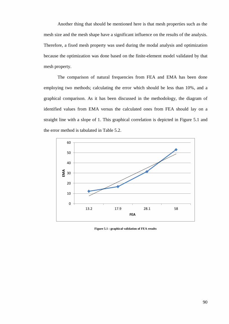
90

Another thing that should be mentioned here is that mesh properties such as the

mesh size and the mesh shape have a significant influence on the results of the analysis.

Therefore, a fixed mesh property was used during the modal analysis and optimization

because the optimization was done based on the finite-element model validated by that

mesh property.

The comparison of natural frequencies from FEA and EMA has been done

employing two methods; calculating the error which should be less than 10%, and a

graphical comparison. As it has been discussed in the methodology, the diagram of

identified values from EMA versus the calculated ones from FEA should lay on a

straight line with a slope of 1. This graphical correlation is depicted in Figure 5.1 and

the error method is tabulated in Table 5.2.

Figure ‎5.1 : graphical validation of FEA results

0

10

20

30

40

50

60

13.2 17.9 28.1 58

EMA

FEA

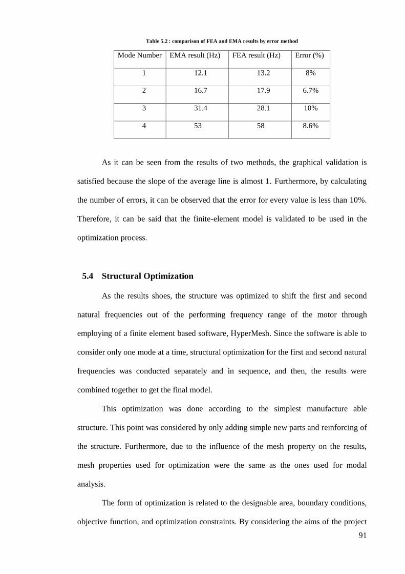
91

Table ‎5.2 : comparison of FEA and EMA results by error method

Mode Number EMA result (Hz) FEA result (Hz) Error (%)

1 12.1 13.2 8%

2 16.7 17.9 6.7%

3 31.4 28.1 10%

4 53 58 8.6%

As it can be seen from the results of two methods, the graphical validation is

satisfied because the slope of the average line is almost 1. Furthermore, by calculating

the number of errors, it can be observed that the error for every value is less than 10%.

Therefore, it can be said that the finite-element model is validated to be used in the

optimization process.


As the results shoes, the structure was optimized to shift the first and second

natural frequencies out of the performing frequency range of the motor through

employing of a finite element based software, HyperMesh. Since the software is able to

consider only one mode at a time, structural optimization for the first and second natural

frequencies was conducted separately and in sequence, and then, the results were

combined together to get the final model.

This optimization was done according to the simplest manufacture able

structure. This point was considered by only adding simple new parts and reinforcing of

the structure. Furthermore, due to the influence of the mesh property on the results,

mesh properties used for optimization were the same as the ones used for modal

analysis.

The form of optimization is related to the designable area, boundary conditions,

objective function, and optimization constraints. By considering the aims of the project

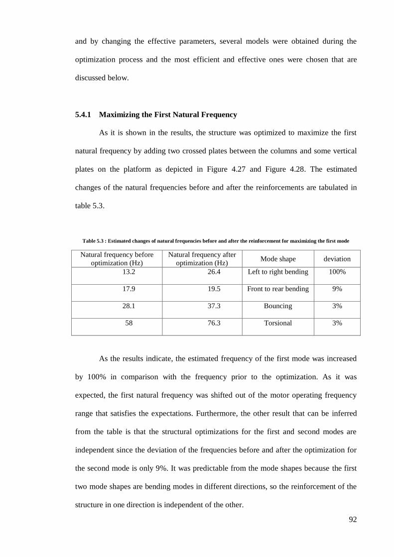
92

and by changing the effective parameters, several models were obtained during the

optimization process and the most efficient and effective ones were chosen that are

discussed below.

5.4.1 Maximizing the First Natural Frequency

As it is shown in the results, the structure was optimized to maximize the first

natural frequency by adding two crossed plates between the columns and some vertical

plates on the platform as depicted in Figure 4.27 and Figure 4.28. The estimated

changes of the natural frequencies before and after the reinforcements are tabulated in

table 5.3.

Table ‎5.3 : Estimated changes of natural frequencies before and after the reinforcement for maximizing the first mode

Natural frequency before

optimization (Hz)

Natural frequency after

optimization (Hz) Mode shape deviation

13.2 26.4 Left to right bending 100%

17.9 19.5 Front to rear bending 9%

28.1 37.3 Bouncing 3%

58 76.3 Torsional 3%

As the results indicate, the estimated frequency of the first mode was increased

by 100% in comparison with the frequency prior to the optimization. As it was

expected, the first natural frequency was shifted out of the motor operating frequency

range that satisfies the expectations. Furthermore, the other result that can be inferred

from the table is that the structural optimizations for the first and second modes are

independent since the deviation of the frequencies before and after the optimization for

the second mode is only 9%. It was predictable from the mode shapes because the first

two mode shapes are bending modes in different directions, so the reinforcement of the

structure in one direction is independent of the other.

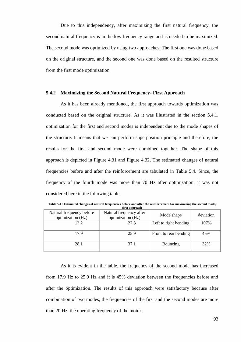
93

Due to this independency, after maximizing the first natural frequency, the

second natural frequency is in the low frequency range and is needed to be maximized.

The second mode was optimized by using two approaches. The first one was done based

on the original structure, and the second one was done based on the resulted structure

from the first mode optimization.

5.4.2 Maximizing the Second Natural Frequency- First Approach

As it has been already mentioned, the first approach towards optimization was

conducted based on the original structure. As it was illustrated in the section 5.4.1,

optimization for the first and second modes is independent due to the mode shapes of

the structure. It means that we can perform superposition principle and therefore, the

results for the first and second mode were combined together. The shape of this

approach is depicted in Figure 4.31 and Figure 4.32. The estimated changes of natural

frequencies before and after the reinforcement are tabulated in Table ‎5.4. Since, the

frequency of the fourth mode was more than 70 Hz after optimization; it was not

considered here in the following table.

Table ‎5.4 : Estimated changes of natural frequencies before and after the reinforcement for maximizing the second mode,

first approach


optimization (Hz)


optimization (Hz) Mode shape deviation



28.1 37.1 Bouncing 32%

As it is evident in the table, the frequency of the second mode has increased

from 17.9 Hz to 25.9 Hz and it is 45% deviation between the frequencies before and

after the optimization. The results of this approach were satisfactory because after

combination of two modes, the frequencies of the first and the second modes are more

than 20 Hz, the operating frequency of the motor.

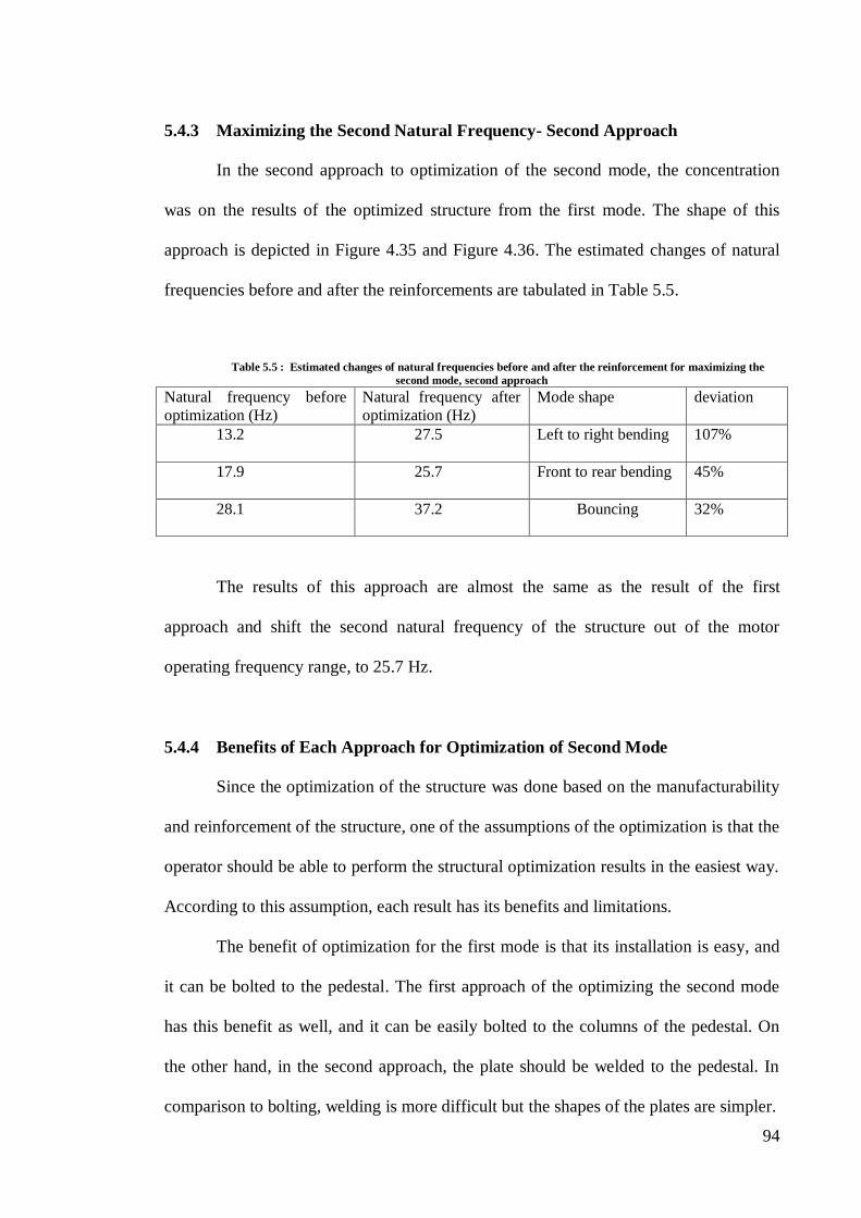
94

5.4.3 Maximizing the Second Natural Frequency- Second Approach

In the second approach to optimization of the second mode, the concentration

was on the results of the optimized structure from the first mode. The shape of this

approach is depicted in Figure 4.35 and Figure 4.36. The estimated changes of natural

frequencies before and after the reinforcements are tabulated in Table 5.5.

Table ‎5.5 : Estimated changes of natural frequencies before and after the reinforcement for maximizing the

second mode, second approach


optimization (Hz)


optimization (Hz)

Mode shape deviation



28.1 37.2 Bouncing 32%

The results of this approach are almost the same as the result of the first

approach and shift the second natural frequency of the structure out of the motor

operating frequency range, to 25.7 Hz.

5.4.4 Benefits of Each Approach for Optimization of Second Mode

Since the optimization of the structure was done based on the manufacturability

and reinforcement of the structure, one of the assumptions of the optimization is that the

operator should be able to perform the structural optimization results in the easiest way.

According to this assumption, each result has its benefits and limitations.

The benefit of optimization for the first mode is that its installation is easy, and

it can be bolted to the pedestal. The first approach of the optimizing the second mode

has this benefit as well, and it can be easily bolted to the columns of the pedestal. On

the other hand, in the second approach, the plate should be welded to the pedestal. In

comparison to bolting, welding is more difficult but the shapes of the plates are simpler.

95

Chapter Six

6 Conclusion and Recommendations

General conclusions of this research are summarized in this chapter.

Furthermore, suggested areas for additional works are introduced.

6.1 Conclusions

The aim of this research was structural dynamic modification of a vibrating

structure by using of the topology optimization method in order to find the most

effective design of a pedestal structure on which an electrical motor is installed. So, by

applying modal testing and ODS measurement, the dynamic characteristics of a

vibrating structure was ascertained. Furthermore, based on topology optimization

method, the optimum design of the structure was determined.

In this work, according to the defined objectives, a structural vibration analysis was

successfully done to get the vibration properties of the structure. At first, a modal

testing and an ODS measurement have been applied on the structure to recognize the

natural frequencies, mode shapes, and exact deflection shape of the structure. The

modal testing showed that the structure has two modes at 12.1 Hz and 16.7 Hz which

are below the assumed motor operating frequency range. The first two mode shapes of

this structure were also determined which are “left to right bending” and “rear to front

bending,” respectively. The ODS measurement showed the exact deflection shapes

related to these natural frequencies. Afterwards, the finite element model of the

structure was verified by comparing with the experimental data. Two parameters were

evaluated for verification of the FEM results: The first one was about the error between

the values obtained from finite element modal analysis and EMA, which were less than

96

10%, and the second one was a direct correlation between the values, which the points

were laid on a straight line with a slope of 1.0. Next, a topological optimization was

applied to get the new structure condition and shape. According to the visual estimation

resulted from topology optimization, the modified structure of the pedestal was

proposed. Then, by applying the FEA modal testing to the new design, it was observed

that both of the natural frequencies shifted from 12.1 Hz and 16.7 Hz to 27.5 Hz and

25.7 Hz, respectively. Accordingly, there would not be any natural frequency under

motor operating frequency range. In addition, the fabrication of this new proposed

design will have an uncomplicated fabrication procedure.

As a conclusion, topology optimization method could be used to find the most

effective design for structural dynamic modification of vibrating structures. Moreover,

less time is needed to achieve to the results compared with trial and error methods.

6.2 Recommendations for Future Works

In this work, the objective function of the optimization was maximizing natural

frequency, and the constraint was the volume fraction. Other works that can be done in

this area can focus on the change in these conditions, i.e. objective function, constraint,

designable area, etc. and a comparison of the results could be presented. Furthermore,

the results of more complicated optimized structure, without considering the

manufacturability of the structure can be compared to the results of this work, and the

efficiency of each model can be further discussed.

97

Bibliography

Agilent. (2008). The fundamentals of modal testing, application note In A.

Technologies (Ed.). U.S.A.

Arora, J. S. (1993). Sequential linearization and quadratic programming techniques. in:

Kamat M. (Ed.). Structural Optimization: Status and Promise, AIAA, 71-102.

Babuska, I. (1976). Solution of interface problems by homogenization I. Journal of

Mathematical Analysis, 7, 603-634.

Bendsøe, M. P., & Kikuchi, N. (1988). Generating optimal topologies in structural

design using a homogenization method. Comp. Meth. Appl. Mech. Eng., 71.

Bendsøe, M. P., & Kikuchi, N. (1988). Generating optimal topologies in structural

design using a homogenization method. Computer Methods in Applied

Mechanics and Engineering, 71, 197-224.

Bendsøe, M. P., & Kikuchi, N. (1989). Optimal shape design as a material distribution

problem. Structural Optimization, 1, 193-202.

Bendsøe, M. P., & Mota Soares, C. A. (1993). Topology design of discrete structures. In

Topology Design of Structures. Netherlands: Kluwer Academic Publishers.

Bendsøe, M. P., & Sigmund, O. (1999). Material interpolation schemes in topology

optimization. Archive of Applied Mechanics, 69.

Bendsøe, M. P., & Sigmund, O. (2003). Topology optimization : theory, methods, and

applications. Berlin ; New York: Springer.

Bulman, S., Sienz, J., & Hinton, E. (2001). Comparisons between algorithms for

structural topology optimization using a series of benchmark studies. Computers

& Structures, 79, 1209-1218.

Cardoso, E. L., & Fonseca, J. O. F. (2003). Complexity control in the topology

optimization of continuum structures. Journal of the Braz. Soc. of Mech. Sci. &

Eng., 3.

Chiat, L. W. (2008). Design and Optimization of a Dynamically-Tuned Vibration

Absorber Using Experimental and Computational Methods. Bachelor’s degree,

University of Malaya.

Chu, D. N. (1997). Evolutionary Structural Optimization Method for Systems with

Stiffness and Displacement Constraints. PhD, Victoria University of

Technology, Melbourne, Australia.

Cioranescu, D., & Paulin, J. S. J. (1979). Homogenization in open sets with holes.

Journal of Math. Analysis and Appl, 71, 590-607.

Diaz , A. R., & Kikuchi, N. (1992). Solutions to shape and topology eigenvalue

optimization problems using a homogenization method. Int. J. Num. Meth.

Engng, 35.

Dobbs, M. W., & Felton, L. P. (1969). Optimization of truss geometry. J. Struct. Div.,

ASCE l00 (STl), 2105-1118.

Dorn, W. C., Gomory, R. E., & Greenberg, H. J. (1964). Automatic design of optimal

structures. J. de Mecanique, 3, 25-52.

Fiacco, A. V., & McCormick, G. P. (1968). Nonlinear programming: sequential

unconstrained minimization techniques. New York: Wiley.

Fleury, C. (1979). Structural weight Optimization by dual methods for convex

programming. International Journal for Numerical Methods in Engineering, 14,

1761-1783.

Haftka, R. T., & Grandhi, R. V. (1986). Structural optimization-a survey. Computer

Methods in Applied Mechanics and Engineering, 57, 91-106.

Haftka, R. T., & Gürdal, Z. (1992). Elements of structural optimization (3rd rev. and

expanded ed.). Dordrecht ; Boston: Kluwer Academic Publishers.

98

Heyman, J. (1951). Plastic design of beams and frames for minimum material

consumption. Quarterly of Applied Mathematics, 8.

Holland, J. H. (1975). Adaptation in national and artificial systems. Ann Arbor, USA:

University of Michigan Press.

Huang, X., & Xie, Y. M. (2010). Evolutionary topology optimization of continuum

structures : methods and applications. Chichester, West Sussex, U.K. ;

Hoboken, NJ: Wiley.

Jensen, J. S., & Pedersen, N. L. (2006). On maximal eigenfrequency separation in two-

material structures: the 1D and 2D scalar cases. [doi:

10.1016/j.jsv.2005.03.028]. Journal of Sound and Vibration, 289(4-5), 967-986.

Jog, C. S. (2002). TOPOLOGY DESIGN OF STRUCTURES SUBJECTED TO

PERIODIC LOADING. [doi: 10.1006/jsvi.2001.4075]. Journal of Sound and

Vibration, 253(3), 687-709.

Jung, E.-I., Park, Y.-S., & Park, K. C. (2005). Structural dynamics modification via

reorientation of modification elements. [doi: 10.1016/j.finel.2005.05.004]. Finite

Elements in Analysis and Design, 42(1), 50-70.

Kang, Z., Wang, X., & Wang, R. (2009). Topology optimization of space vehicle

structures considering attitude control effort. [doi: 10.1016/j.finel.2008.12.002].

Finite Elements in Analysis and Design, 45(6-7), 431-438.

Kirsch, U. (1989). Optimal topologies of Structures. Appl. Mech. Rev, 42, 223-239.

Krog, L. A., & Olhoff, N. (1999). Optimum topology and reinforcement design of disk

and plate structures with multiple stiffness and eigenfrequency objectives. [doi:

10.1016/S0045-7949(98)00326-5]. Computers & Structures, 72(4-5), 535-563.

Ma, Z. D., Cheng, H.-C., & Kikuchi, N. (1994). Structural design for obtaining desired

eigenfrequencies by using the topology and shape optimization method. [doi:

10.1016/0956-0521(94)90039-6]. Computing Systems in Engineering, 5(1), 77-

89.

Ma, Z. D., Kikuchi, N., & Cheng, H. C. (1995). Topology design for vibrating

structures. Computer Methods in Applied Mechanics and Engineering, 121, 259-

280.

Maxwell, C. (1895). Scientific Papers II: Cambridge University Press.

Michell, A. G. M. (1904). The limit of economy of material in frame-structures.

Molter, A., Fonseca, J. S. O., Bottega, V., & Alves da Silveira, O. A. (2010).

Simultaneous topology optimization and optimal control for vibration suppression in structural design. Paper presented at the 2nd International

Conference on Engineering Optimization, Lisbon, Portugal.

Molter, A., Fonseca, J. S. O., Bottega, V., Otávio, A., & Silveira, d. (2010).

Simultaneous topology optimization and optimal control for vibration suppression in structural sesign. Paper presented at the 2nd International

Conference on Engineering Optimization, Lisbon, Portugal.

Nagendra, S., Haftka, R. T., & Giirdal, Z. (1993). Design of blade stiffened composite

panels by a genetic algorithm approach. Paper presented at the Proceedings of

the 34th AlAA/ASME/AHS SDM Conference, La Jolla, USA.

Olhoff, N., Bendsoe, M. P., & Rasmussen, J. (1991). On CAD-integrated structural

topology and design optimization. Comp. Meth. Appl. Mech. Engrg., 89.

Ou, J. S., & Kikuchi, N. (1996). Integrated optimal structural and vibration control

design. Structural Optimization, 12.

Prager, W., & J.E., T. (1968). Problems of optimal structural design. Journal of Applied

Mechanics, 35, 102-106.

Prager, W., & Shield, R. T. (1968). Optimal design of multi-purpose structures. Int. J.

Solids and Structures, 4, 469-475.

99

Ramli, R. (1998). Structure-borne Noise Problems in a Passenger Car. Master,

University of Malaya.

Richardson, M. H. (1997). Is It a Mode Shape, or an Operating Deflection Shape? (Vol.

30th Anniversary). Jamestown, California: Vibrant Technology, Inc.

Rong, J. H., Xie, Y. M., Yang, X. Y., & Liang, Q. Q. (2001). Topology optimization of

structures under dynamic response constraints. Sound & Vibration, 23(4), 177-

189.

Rosen, J. B. (1961). The gradient projection method for nonlinear programming.

Journal of the Society for Industrial and Applied Mathematics, 8.

Rozvany, G. I. N. (1995). What is meaningful in topology design? An engineer’s

viewpoint, Advances in Structural Optimization. Netherlands: Kluwer Academic

Publishers.

Schedlinski, c., Wagner, F., Bohnert, K., Frappier, J., Irrgang, A., Lehmann, R., &

Muller, A. (2004). experimental modal analysis and computational model

updating of a car body in white. Paper presented at the ISMA 2004, Leuven,

Belgium.

Schmit, L. A. (1960). Structural design by systematic synthesis. Paper presented at the

Proceedings of the 2nd conference on Electronic Computation, New York.

Schwarz, B. J., & Richardson, M. H. (1999). Experimental Modal Analysis. Vibrant

Technology, Inc. Schwarz, B. J., & Richardson, M. H. (1999). Introduction to operating deflection

shapes. Vibrant Technology, Inc.

Taylor. (1977). Optimal truss design based on an algorithm using optimality criteria.

Int. J. Solids Struct, 13, 913-923.

Tenek, L. H., & Hagiwara, I. (1993). Static and vibrational shape and topology

optimization using homogenization and mathematical programming. Computer

Methods in Applied Mechanics and Engineering, 109, 143-154.

Venkayya, V. B., Khot, N. S., & Reddy, V. S. (1968). Optimization of structures based

on the study of strain energy distribution. Paper presented at the DTIC.

Xie, Y. M., & Steven, G. P. (1993). A simple evolutionary procedure for structural

Optimization. Computers and Structures, 49, 885-896.

Xie, Y. M., & Steven, G. P. (1994). Optimal design of multiple load case structures

using an evolutionary procedure. Engineering Computations, 11, 295-302.

Yoon, G. H. (2010). Maximizing the fundamental eigenfrequency of geometrically

nonlinear structures by topology optimization based on element connectivity

parameterization. [doi: 10.1016/j.compstruc.2009.07.006]. Computers &

Structures, 88(1-2), 120-133.

Zhao, C., Steven, G. P., & Xie, Y. M. (1998). A generalized evolutionary method for

natural frequency optimization of membrane vibration problems in finite

element analysis. [doi: 10.1016/S0045-7949(97)00054-0]. Computers &

Structures, 66(2-3), 353-364.

Zhou, M., & Rozvany, G. I. N. (1991). The COG algorithm, Part II: Topological,

geometrical and general shape optimization. Comp. Meth. Appl. Mech. Eng., 89,

309-336.

Zoutendijk, G. (1960). Methods for Feasible Direction. Amsterdam: Elsevier.

Date post:	30-Aug-2019
Category:	Documents
Upload:	others
View:	6 times
Download:	0 times

STRUCTURAL DYNAMIC MODIFICATION OF VIBRATING...

Documents