Department of Data Analysis Ghent University Structural Equation Modeling with lavaan Yves Rosseel Department of Data Analysis Ghent University CISA – Gen` eve 31 Januari 2020 Yves Rosseel Structural Equation Modeling with lavaan 1/ 151
Transcript
Department of Data Analysis Ghent University
Structural Equation Modeling with lavaan
Yves RosseelDepartment of Data Analysis
Ghent University
CISA – Geneve31 Januari 2020
Yves Rosseel Structural Equation Modeling with lavaan 1 / 151
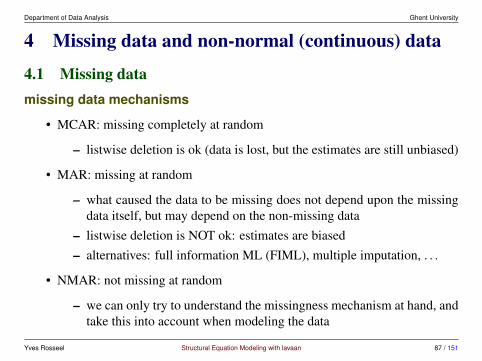
4 Missing data and non-normal (continuous) data 874.1 Missing data . . . . . . . . . . . . . . . . . . . . . . . . . . . . . 874.2 Nonnormal data and alternative estimators . . . . . . . . . . . . . 92
5 Categorical data 1025.1 Handling categorical endogenous variables . . . . . . . . . . . . 1025.2 Two approaches for handling categorical data in a SEM framework 1035.3 A limited information approach: the WLSMV estimator . . . . . . 104
Yves Rosseel Structural Equation Modeling with lavaan 6 / 151
Department of Data Analysis Ghent University
multivariate regression
x1
x2
x3
x4
y1
y2
• strict distinction between ‘dependent’ variables and ‘independent’ variables
Yves Rosseel Structural Equation Modeling with lavaan 7 / 151
Department of Data Analysis Ghent University
path analysis
• all variables are observed (manifest)
• we allow for indirect effects (eg., of y5, via y6 on y7)
• we allow for cycles (eg. y7 could influence y5)
y1
y2
y3
y4
y5
y6 y7
y5 = reading motivation
y6 = reading frequency
y7 = reading ability
Yves Rosseel Structural Equation Modeling with lavaan 8 / 151
Department of Data Analysis Ghent University
confirmatory factor analysis (CFA)
• measurement model: representing the relationship between one or more la-tent variables and their (observed) indicators
y1
y2
y3
y4
y5
y6
η1
η2
η1 = depression
η2 = neuroticism
Yves Rosseel Structural Equation Modeling with lavaan 9 / 151
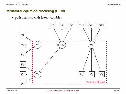
Department of Data Analysis Ghent University
structural equation modeling (SEM)
• path analysis with latent variables
y1
y2
y3
y4
y5
y6
η1
η2
y7 y8 y9 y10 y11 y12
x1 x2 x3
η3 η4
structural part
Yves Rosseel Structural Equation Modeling with lavaan 10 / 151
Department of Data Analysis Ghent University
1.2 How does SEM work?a dataset: the Holzinger & Swineford dataset
• this is a ‘classic’ dataset, based on data collected by Holzinger & Swineford(1939)
• scores on 26 ‘Mental Ability tests’ of seventh- and eighth-grade childrenfrom two different schools (Pasteur and Grant-White)
• the dataset was used in a seminal paper about CFA (Joreskog, 1969)
• just like Joreskog (1969), we will use a subset of 9 scores: x1 = Visualperception, x2 = Cubes, x3 = Lozenges, x4 = Paragraph comprehension, x5= Sentence completion, x6 = Word meaning, x7 = Speeded addition, x8 =Speeded counting of dots, x9 = Speeded discrimination
• these 9 scores are often regarded as indicators of 3 latent variables: ‘visualintelligence’ (x1, x2, x3), ‘textual intelligence’ (x4, x5, x6), en ‘speed’ (x7,x8, x9)
• we will investigate this later using CFA
Yves Rosseel Structural Equation Modeling with lavaan 11 / 151
Department of Data Analysis Ghent University
reading in data + descriptives> library(lavaan)> dim(HolzingerSwineford1939)
computing the variance-covariance matrix for P = 9 variables> N <- nrow(HolzingerSwineford1939)> S <- cov( HolzingerSwineford1939[, var.names] )> S <- S * (N-1)/N # ML version> round(S, 3)
Yves Rosseel Structural Equation Modeling with lavaan 13 / 151
Department of Data Analysis Ghent University
the model-implied variance-covariance matrix
• the goal of SEM is to test an a priori specified theory/model, based on em-pirical data; we would like to know if our model ‘fits’ the data (or not)
• each model can be depicted by a path diagram (we may have several alter-native models, each one with its own path diagram)
• each path diagram can be converted to a SEM
• SEM will tell us what the implications are for the data if (assumption!) ourmodel is correct: how ‘should’ the data look like, which patterns should weobserve?
• in practice, SEM will tell us how the variance-covariance matrix of the datashould look like; we call this the ‘model-implied’ variance-covariance ma-trix (Σ)
• different models→ different path diagrams→ different Σ matrices
• if Σ is close to S, the model fits well
Yves Rosseel Structural Equation Modeling with lavaan 14 / 151
Department of Data Analysis Ghent University
example model-implied covariance matrix (1)
• suppose we have three observed (random) variables, y1, y2 and y3; to explainwhy they are correlated, we may postulate the following model:
y1 y2
y3
a
b
y2 = a y1 + ε2
y3 = b y1 + ε3
• suppose, we set a = 3 en b = 5, Var(y1) = 10, Var(ε2) = 20, Var(ε3) = 30;then, it can be shown that the model-implied variance-covariance matrixequals
Σ =
10
30 110
50 150 280
Yves Rosseel Structural Equation Modeling with lavaan 15 / 151
Department of Data Analysis Ghent University
example model-implied covariance matrix (2)
• but if we change the path diagram (and keep the parameter values fixed), themodel-implied covariance matrix will also change:
y1 y2
y3
a
b
we find
Σ =
10
30 110
150 550 2780
• two models are said to be equivalent, if they imply the same covariance
matrix (but note that we did not estimate the parameters here)
Yves Rosseel Structural Equation Modeling with lavaan 16 / 151
Department of Data Analysis Ghent University
example model-implied covariance matrix (3)
• we can also postulate that the correlations among the three observed vari-ables are explained by a common ‘factor’:
y1
y2
y3
η
1
a
b
• we find using σ2(ε1) = 10, σ2(ε2) = 20, σ2(ε3) = 30, σ2(η) = 1:
Σ =
11
4 36
5 20 55
• we can compare all three Σ matrices to S to find out which model fits best
Yves Rosseel Structural Equation Modeling with lavaan 17 / 151
Department of Data Analysis Ghent University
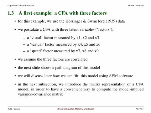
1.3 A first example: a CFA with three factors• for this example, we use the Holzinger & Swineford (1939) data
• we postulate a CFA with three latent variables (‘factors’):
– a ‘visual’ factor measured by x1, x2 and x3
– a ‘textual’ factor measured by x4, x5 and x6
– a ‘speed’ factor measured by x7, x8 and x9
• we assume the three factors are correlated
• the next slide shows a path diagram of this model
• we will discuss later how we can ‘fit’ this model using SEM software
• in the next subsection, we introduce the matrix representation of a CFAmodel, in order to have a convenient way to compute the model-impliedvariance-covariance matrix
Yves Rosseel Structural Equation Modeling with lavaan 18 / 151
Department of Data Analysis Ghent University
diagram of the model
x1
x2
x3
x4
x5
x6
x7
x8
x9
visual
textual
speed
• ‘free’ parameters: factor loadings, variances for the factors, covariances be-tween the factors, and residual variances for the indicators
Yves Rosseel Structural Equation Modeling with lavaan 19 / 151
Department of Data Analysis Ghent University
1.4 The matrix representation of a CFA model• the classic LISREL representation uses three model matrices for a CFA
• the LAMBDA matrix contains the ‘factor structure’:
Λ =
x 0 0
x 0 0
x 0 0
0 x 0
0 x 0
0 x 0
0 0 x
0 0 x
0 0 x
• the variances/covariances of the latent variables are summarized in the PSI
matrix:
Yves Rosseel Structural Equation Modeling with lavaan 20 / 151
Department of Data Analysis Ghent University
Ψ =
x
x x
x x x
• what we can not explain by the set of common factors (the ‘residual part’ of
the model) is written in the (typically diagonal) matrix THETA:
Θ =
x
x
x
x
x
x
x
x
x
• note that we have only 24 parameters (of which 21 are estimable)
Yves Rosseel Structural Equation Modeling with lavaan 21 / 151
Department of Data Analysis Ghent University
the standard CFA model: the model implied covariance matrix
• in the standard CFA model, the ‘implied’ covariance matrix is:
Σ = ΛΨΛ′ + Θ
• all parameters are included in three model matrices
• simple matrix multiplication (and addition) gives us the model implied co-variance matrix
• for identification purposes, some parameters need to be fixed to a constant(see next slide)
• estimation problem: choose the ‘free’ parameters, so that the estimated im-plied covariance matrix (Σ) is ‘as close as possible’ to the observed covari-ance matrix S
Yves Rosseel Structural Equation Modeling with lavaan 22 / 151
Department of Data Analysis Ghent University
setting the metric of the latent variables: UVI of ULI
1. Unit Loading Identification (ULI):the factor loading of one (often the first) of the indicators is fixed to 1.0; thisindicator is called the reference indicator
2. Unit Variance Identification (UVI):the variance of the factor is fixed to 1.0
y1
y2
y3
η1
1
?
?
y1
y2
y3
η1
1.0?
?
?
• in many models, it does not matter
• in multigroup SEM analysis: we usually use ULI
Yves Rosseel Structural Equation Modeling with lavaan 23 / 151
Department of Data Analysis Ghent University
number of free parameters and degrees of freedom
• in our example, we have used ULI: the first factor loading (of each latentvariable) was fixed to 1.0
• therefore, we only have 21 free parameters in our model:
– 6 factor loadings– 3 variances for the factors– 3 covariances between the factors– 9 residual variances for the indicators
• our sample variance-covariance matrix (S) contains P (P +1)/2 = 45 (non-redundant) elements (‘sample statistics’)
• the difference between the number of sample statistics and the number offree parameters is called the ‘degrees of freedom’ of the model; for thismodel, we have 45− 21 = 24 degrees of freedom (df = 24)
• the number of free parameters cannot exceed the number of sample statistics;if df = 0, we say the model is ‘saturated’ because in this case Σ = S
Yves Rosseel Structural Equation Modeling with lavaan 24 / 151
Department of Data Analysis Ghent University
1.5 A second example: the Political Democracy dataset• data from N = 75 developing countries regarding the amount of ‘industrial-
ization’ (in 1960) and the level of ‘political democracy’ (in 1960, and againin 1965)
• this dataset is used throughout Bollen’s 1989 book
• overview of the observed variables (indicators):
y1: Expert ratings of the freedom of the press in 1960y2: The freedom of political opposition in 1960y3: The fairness of elections in 1960y4: The effectiveness of the elected legislature in 1960y5: Expert ratings of the freedom of the press in 1965y6: The freedom of political opposition in 1965y7: The fairness of elections in 1965y8: The effectiveness of the elected legislature in 1965x1: The gross national product (GNP) per capita in 1960x2: The inanimate energy consumption per capita in 1960x3: The percentage of the labor force in industry in 1960
• three latent variables: ind60, measured by x1, x2 and x3; dem60, mea-sured by y1, y2, y3 and y4; dem65 measured by y5, y6, y7 en y8
Yves Rosseel Structural Equation Modeling with lavaan 25 / 151
Department of Data Analysis Ghent University
model diagram
y1
y2
y3
y4
y5
y6
y7
y8
x1 x2 x3
dem60
dem65
ind60
Yves Rosseel Structural Equation Modeling with lavaan 26 / 151
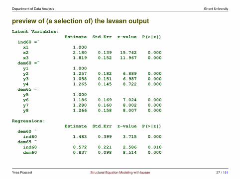
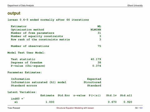
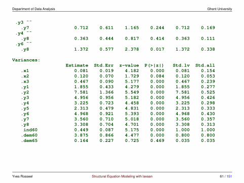
Department of Data Analysis Ghent University
preview of (a selection of) the lavaan outputLatent Variables:
• there is a lot of controversy about the use (and misuse) of these fit indices
• a good reference is still Hu & Bentler (1999)
• current practice is to report: chi-square value + df + pvalue, RMSEA, CFIand SRMR (do not cherry pick your fit indices)
Yves Rosseel Structural Equation Modeling with lavaan 30 / 151
Department of Data Analysis Ghent University
evaluation of fit – new developments
• renewed attention for SRMR; see for example
Maydeu-Olivares, A. (2017). Assessing the size of model misfitin structural equation models. Psychometrika, 82, 533–558
• the SRMR is (more or less) the ‘average’ of the (standardized) squared resid-uals (e.g., between the elements of S and Σ); the CRMR converts first tocorrelation matrices
• unlike other fit measures, SRMR/CRMR has a straightforward interpretation
• an unbiased estimate is available, as well as a standard error, and a confi-dence interval
• another approach is to focus on ‘local’ fit measures: looking at just one partof the model; see for example
Thoemmes, F., Rosseel, Y., & Textor, J. (2018). Local fit evalu-ation of structural equation models using graphical criteria. Psy-chological methods, 23, 27–41.
Yves Rosseel Structural Equation Modeling with lavaan 31 / 151
Department of Data Analysis Ghent University
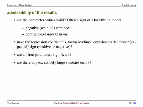
admissibility of the results
• are the parameter values valid? Often a sign of a bad-fitting model
– negative (residual) variances
– correlations larger than one
• have the regression coefficients, factor loadings, covariances the proper (ex-pected) sign (positive or negative)?
• are all free parameters significant?
• are there any excessively large standard errors?
Yves Rosseel Structural Equation Modeling with lavaan 32 / 151
Department of Data Analysis Ghent University
1.8 Model respecification• if the fit of a model is not good, we can adapt (respecify) the model
– change the number of factors
– allow for indicators to be related to more than one factor (cross-loadings)
– allow for correlated residual errors among the observed indicators
– allow for correlated disturbances among the endogenous latent vari-ables
– remove problematic indicators . . .
• ideally, all changes should have a sound theoretical justification
• of course, we may let the data speak for itself, and have a look at the modi-fication indices (a more explorative approach)
Yves Rosseel Structural Equation Modeling with lavaan 33 / 151
Department of Data Analysis Ghent University
1.9 Reporting your results• see Boomsma (2000)
• report enough information so that the analysis can be replicated
– always report the observed covariance matrix (or the correlation matrix+ standard deviations)
– or make sure the full dataset is available (either as an electronic ap-pendix or via a website)
Yves Rosseel Structural Equation Modeling with lavaan 34 / 151
Department of Data Analysis Ghent University
1.10 Further readingKline, R. B. (2015). Principles and practice of structural equation modeling (FourthEdition). New York: Guilford Press.
. . . The companion website supplies data, syntax, and output for the book’sexamples–now including files for Amos, EQS, LISREL, Mplus, Stata, and R(lavaan).
Brown, T. A. (2015). Confirmatory Factor Analysis for Applied Research (SecondEdition) New York: Guilford Press.
Bollen, K.A. (1989). Structural equations with latent variables. New York: Wiley.
Hancock, G. R., & Mueller, R. O. (Eds.). (2013). Structural equation modeling: Asecond course (Second Edition). Greenwich, CT: Information Age Publishing, Inc.
Boomsma, A. (2000). Reporting Analyses of Covariance Structures. StructuralEquation Modeling: A Multidisciplinary Journal, 7, 461–483.
Yves Rosseel Structural Equation Modeling with lavaan 35 / 151
Department of Data Analysis Ghent University
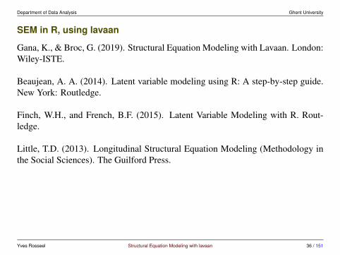
SEM in R, using lavaan
Gana, K., & Broc, G. (2019). Structural Equation Modeling with Lavaan. London:Wiley-ISTE.
Beaujean, A. A. (2014). Latent variable modeling using R: A step-by-step guide.New York: Routledge.
Finch, W.H., and French, B.F. (2015). Latent Variable Modeling with R. Rout-ledge.
Little, T.D. (2013). Longitudinal Structural Equation Modeling (Methodology inthe Social Sciences). The Guilford Press.
Yves Rosseel Structural Equation Modeling with lavaan 36 / 151
Department of Data Analysis Ghent University
2 Introduction to lavaan
2.1 Software for SEMsoftware for SEM: commercial – closed-source
• outside the R ecosystem: gllamm (Stata), Onyx, . . .
• R packages: sem, OpenMx, lavaan, lava
Yves Rosseel Structural Equation Modeling with lavaan 37 / 151
Department of Data Analysis Ghent University
2.2 The R package ‘lavaan’what is lavaan?
• lavaan is an R package for latent variable analysis:
– general mean/covariance structure modeling: function lavaan()– user-friendly interface: function sem() or cfa()– support for continuous, binary and ordinal data– support for missing data, multiple groups, clustered data, . . .
• under development, future plans:
– EFA, ESEM, mixture/latent-class SEM, IRT, new engine, . . .
• the long-term goal of lavaan is
1. to implement all the state-of-the-art capabilities that are currently avail-able in commercial packages
2. to provide a modular and extensible platform that allows for easy im-plementation and testing of new statistical and modeling ideas
Yves Rosseel Structural Equation Modeling with lavaan 38 / 151
Department of Data Analysis Ghent University
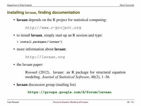
installing lavaan, finding documentation
• lavaan depends on the R project for statistical computing:
http://www.r-project.org
• to install lavaan, simply start up an R session and type:
> install.packages("lavaan")
• more information about lavaan:
http://lavaan.org
• the lavaan paper:
Rosseel (2012). lavaan: an R package for structural equationmodeling. Journal of Statistical Software, 48(2), 1–36.
• lavaan discussion group (mailing list)
https://groups.google.com/d/forum/lavaan
Yves Rosseel Structural Equation Modeling with lavaan 39 / 151
Department of Data Analysis Ghent University
the lavaan ecosystem
• blavaan (Ed Merkle, Yves Rosseel)
Bayesian SEM (using jags or stan) with a lavaan interface
• lavaan.survey (Daniel Oberski)
survey weights, clustering, strata, and finite sampling correctionsin SEM
• Onyx (Timo von Oertzen, Andreas M. Brandmaier, Siny Tsang)
interactive graphical interface for SEM (written in Java)
• semTools (Terrence Jorgensen and many others)
collection of useful functions for SEM
• simsem (Terrence Jorgensen and many others)
simulation of SEM models
Yves Rosseel Structural Equation Modeling with lavaan 40 / 151
Department of Data Analysis Ghent University
the lavaan ecosystem (2)
• semPlot (Sacha Epskamp)
visualizations of SEM models
• EffectLiteR (Axel Mayer, Lisa Dietzfelbinger)
using SEM to estimate average and conditional effects
• MIIVsem (Zachary Fisher, Kenneth Bollen, and others)
Functions for estimating structural equation models using instru-mental variables.
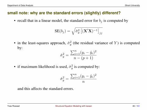
Residual standard error: 46.74 on 95 degrees of freedomMultiple R-squared: 0.5911, Adjusted R-squared: 0.5738F-statistic: 34.33 on 4 and 95 DF, p-value: < 2.2e-16
Yves Rosseel Structural Equation Modeling with lavaan 43 / 151
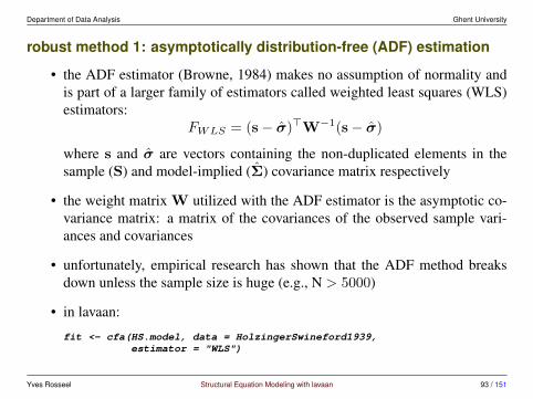
• the ADF estimator (Browne, 1984) makes no assumption of normality andis part of a larger family of estimators called weighted least squares (WLS)estimators:
FWLS = (s− σ)>W−1(s− σ)
where s and σ are vectors containing the non-duplicated elements in thesample (S) and model-implied (Σ) covariance matrix respectively
• the weight matrix W utilized with the ADF estimator is the asymptotic co-variance matrix: a matrix of the covariances of the observed sample vari-ances and covariances
• unfortunately, empirical research has shown that the ADF method breaksdown unless the sample size is huge (e.g., N > 5000)
• in lavaan:
fit <- cfa(HS.model, data = HolzingerSwineford1939,estimator = "WLS")
Yves Rosseel Structural Equation Modeling with lavaan 93 / 151
Department of Data Analysis Ghent University
robust method 2: robust ML
1. parameter estimates: vanilla ML
• if ML is used, the parameter estimates are still consistent (if the modelis identified and correctly specified)
2. ‘robust’ standard errors
• if data is non-normal, the standard errors tend to be too small (as muchas 25-50%)
• ‘robust’ standard errors correct for non-normality
3. ‘robust’ scaled (chi-square) test statistic
• if data is non-normal, the usual model (chi-square) test statistic tendsto be too large
• the Satorra-Bentler scaled test statistic rescales the value of the ML-based chi-square test statistic by an amount that reflects the degree ofkurtosis
Yves Rosseel Structural Equation Modeling with lavaan 94 / 151
Department of Data Analysis Ghent University
robust ML in lavaan
• robust standard errorsfit <- cfa(HS.model, data = HolzingerSwineford1939,
se = "robust")
• Satorra-Bentler scaled test statisticfit <- cfa(HS.model, data = HolzingerSwineford1939,
test = "Satorra-Bentler")
• robust standard errors + scaled test statisticfit <- cfa(HS.model, data = HolzingerSwineford1939,
se = "robust", test = "Satorra-Bentler")
• estimator MLM = robust standard errors + scaled test statisticfit <- cfa(HS.model, data = HolzingerSwineford1939,
estimator = "MLM")
• alternative: estimator MLR (also for missing data)fit <- cfa(HS.model, data = HolzingerSwineford1939,
estimator = "MLR", missing = "ml")
Yves Rosseel Structural Equation Modeling with lavaan 95 / 151
Yves Rosseel Structural Equation Modeling with lavaan 97 / 151
Department of Data Analysis Ghent University
robust method 3: bootstrapping
1. parameter estimates: vanilla ML
2. bootstrapping standard errors
• for the standard errors, we can use the usual nonparametric bootstrap:
(a) take a bootstrap sample (random selection of cases with replace-ment)
(b) fit the model using this bootstrap sample(c) extract the t estimated values of the free parameters(d) repeat steps 1–3 R times (typically, R > 1000)
• collect all these values in a matrix of size R× t• the bootstrap standard errors are the square root of the diagonal ele-
ments of the covariance matrix of this R× t matrix
Yves Rosseel Structural Equation Modeling with lavaan 98 / 151
Department of Data Analysis Ghent University
3. bootstrapping the test statistic
• for the test statistic, we can not use the usual nonparametric bootstrap,because it reflects not only non-normality and sampling variability, butalso model misfit
• the original sample must first be transformed so that the sample covari-ance matrix corresponds with the model-implied covariance matrix
• in the SEM literature, this model-based bootstrap procedure is knownas the Bollen-Stine bootstrap
• the standard p value of the chi-square test can be replaced by a boot-strap p value: the proportion of test statistics from the bootstrap sam-ples that exceed the value of the test statistic from the original (parent)sample
Yves Rosseel Structural Equation Modeling with lavaan 99 / 151
Department of Data Analysis Ghent University
bootstrapping in lavaan
• bootstrapping standard errors:
fit <- cfa(HS.model, data = HolzingerSwineford1939,se = "bootstrap", verbose = TRUE, bootstrap = 1000)
• bootstrapping the test statistic
fit <- cfa(HS.model, data = HolzingerSwineford1939,test = "bootstrap", verbose = TRUE, bootstrap = 1000)
• when we use se = ”bootstrap”, the parameterEstimates() output will containbootstrap based confidence intervals
Yves Rosseel Structural Equation Modeling with lavaan 100 / 151
Department of Data Analysis Ghent University
using bootstrapLavaan() to compute the Bollen-Stine p-value (optional)fit <- cfa(HS.model, data = HolzingerSwineford1939, se = "none")
# get the test statistic for the original sample
T.orig <- fitMeasures(fit, "chisq")
# bootstrap to get bootstrap test statistics# we only generate 10 bootstrap sample in this example; in practice# you may wish to use a much higher number
• categorical exogenous covariates; eg. gender, country
• we simply need to construct ‘dummy variables’ and proceed as usual
• just like in ordinary regression
categorical endogenous variables
• need special treatment
• binary data, ordinal (ordered) data
• censored data, limited dependent data
• count data, nominal (unordered) data, . . .
Yves Rosseel Structural Equation Modeling with lavaan 102 / 151
Department of Data Analysis Ghent University
5.2 Two approaches for handling categorical data in a SEMframework
• limited information approach
– only univariate and bivariate information is used– estimation often proceeds in two or three stages; the first stages use
maximum likelihood, the last stage uses (weighted) least squares– mainly developed in the SEM literature– perhaps the best known implementation is in Mplus (WLSMV)
• full information approach
– all information is used– most practical: marginal maximum likelihood estimation– requires numerical integration (number of dimensions = number of la-
tent variables)– mainly developed in the IRT literature (and GLMM literature)– only recently incorporated in modern SEM software
Yves Rosseel Structural Equation Modeling with lavaan 103 / 151
Department of Data Analysis Ghent University
5.3 A limited information approach: the WLSMV estimator• developed by Bengt Muthen, in a series of papers; the seminal paper is
Muthen, B. (1984). A general structural equation model withdichotomous, ordered categorical, and continuous latent variableindicators. Psychometrika, 49, 115–132
• this approach has been the ‘golden standard’ in the SEM literature
• first available in LISCOMP (Linear Structural Equations using a Compre-hensive Measurement Model), distributed by SSI, 1987 – 1997
• follow up program: Mplus (Version 1: 1998), currently version 8
• other authors (Joreskog 1994; Lee, Poon, Bentler 1992) have proposed sim-ilar approaches (implemented in LISREL and EQS respectively)
• another great program: MECOSA (Arminger, G., Wittenberg, J., Schepers,A.) written in the GAUSS language (mid 90’s)
Yves Rosseel Structural Equation Modeling with lavaan 104 / 151
Department of Data Analysis Ghent University
stage 1 – estimating the thresholds
• an observed variable y can often be viewed as a partial observation of a latentcontinuous response y?; eg ordinal variable withK = 4 response categories:
latent continuous response y*
−1.4 0.8 1.8
0.0
0.1
0.2
0.3
0.4
y=1 y=2 y=3 y=4
t1
t2
t3
Yves Rosseel Structural Equation Modeling with lavaan 105 / 151
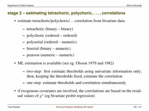
• estimate tetrachoric/polychoric/. . . correlation from bivariate data:
– tetrachoric (binary – binary)
– polychoric (ordered – ordered)
– polyserial (ordered – numeric)
– biserial (binary – numeric)
– pearson (numeric – numeric)
• ML estimation is available (see eg. Olsson 1979 and 1982)
– two-step: first estimate thresholds using univariate information only;then, keeping the thresholds fixed, estimate the correlation
– one-step: estimate thresholds and correlation simultaneously
• if exogenous covariates are involved, the correlations are based on the resid-ual values of y? (eg bivariate probit regression)
Yves Rosseel Structural Equation Modeling with lavaan 106 / 151
Department of Data Analysis Ghent University
stage 3 – estimating the SEM model
• third stage uses weighted least squares:
FWLS = (s− σ)>W−1(s− σ)
where s and σ are vectors containing all relevant sample-based and model-based statistics respectively
• s contains: thresholds, correlations, optionally regression slopes of exoge-nous covariates, optionally variances and means of continuous variables
• the weight matrix W is (a consistent estimator of) the asymptotic covariancematrix of the sample statistics (s)
• robust version: WLSMV
– use the diagonal of W only for estimation (DWLS)– use the full matrix for inference (standard errors and test statistic)– ‘MV’ stands for the Satterthwaite’s mean and variance corrected test
statistic
Yves Rosseel Structural Equation Modeling with lavaan 107 / 151
– combines ‘mixed models’ with path analysis and latent variables– allows for unbalanced data– relatively new, active research; major software package: Mplus
Yves Rosseel Structural Equation Modeling with lavaan 114 / 151
Department of Data Analysis Ghent University
6.1 Repeated measures ANOVA, using SEM• we can mimic the classical repeated measures ANOVA in a SEM framework
• using two time-points only, this is the SEM equivalent of the paired t-test
• but we can relax the compound symmetry restriction
– we can allow for an unstructured covariance structure
– or we could impose an autoregressive AR(1) structure
– . . .
• but above all, we can replace the observed variables by latent variables
Yves Rosseel Structural Equation Modeling with lavaan 115 / 151
Department of Data Analysis Ghent University
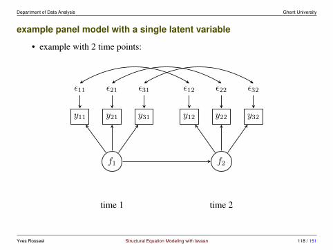
repeated measures using latent variables
• example with 2 time points:
y11 y21 y31 y12 y22 y32
ε11 ε21 ε31 ε12 ε22 ε32
f1 f2
time 1 time 2
Yves Rosseel Structural Equation Modeling with lavaan 116 / 151
Department of Data Analysis Ghent University
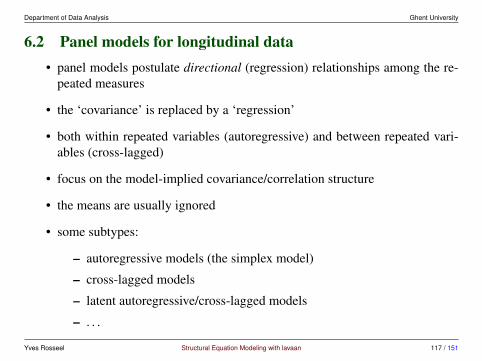
6.2 Panel models for longitudinal data• panel models postulate directional (regression) relationships among the re-
peated measures
• the ‘covariance’ is replaced by a ‘regression’
• both within repeated variables (autoregressive) and between repeated vari-ables (cross-lagged)
• focus on the model-implied covariance/correlation structure
• the means are usually ignored
• some subtypes:
– autoregressive models (the simplex model)
– cross-lagged models
– latent autoregressive/cross-lagged models
– . . .
Yves Rosseel Structural Equation Modeling with lavaan 117 / 151
Department of Data Analysis Ghent University
example panel model with a single latent variable
• example with 2 time points:
y11 y21 y31 y12 y22 y32
ε11 ε21 ε31 ε12 ε22 ε32
f1 f2
time 1 time 2
Yves Rosseel Structural Equation Modeling with lavaan 118 / 151
Department of Data Analysis Ghent University
autoregressive models
• each time point is regressed on a previous time point (first order) , or an evenfurther time point (second order, third order, . . . )
• earliest development dates back to the seminal work of Guttman (1954)
• example first-order univariate autoregressive model:
y1 y2 y3 y4
ε2 ε3 ε4
? ? ?
Yves Rosseel Structural Equation Modeling with lavaan 119 / 151
Department of Data Analysis Ghent University
multivariate panel models
• in a multivariate panel model, we have more than one outcome, measured at(the same) t time points
• example: a bivariate panel/simplex model where Y is a measure of mathe-matical achievement, and Z is a measure of reading ability (4 time points:grade 3, grade 4, grade 5 and grade 6)
y1 y2 y3 y4
z1 z2 z3 z4
ε21 ε31 ε41
ε22 ε32 ε43
Yves Rosseel Structural Equation Modeling with lavaan 120 / 151
Department of Data Analysis Ghent University
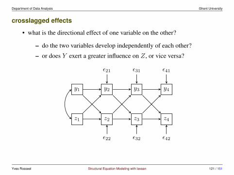
crosslagged effects
• what is the directional effect of one variable on the other?
– do the two variables develop independently of each other?
– or does Y exert a greater influence on Z, or vice versa?
y1 y2 y3 y4
z1 z2 z3 z4
ε21 ε31 ε41
ε22 ε32 ε42
Yves Rosseel Structural Equation Modeling with lavaan 121 / 151
Department of Data Analysis Ghent University
contemporaneous effects
• sometimes, the crossed effects between two variables are not lagged, butcontemporaneous (exerting an effect at the same time point)
• this can be unidirectional, or reciprocal
• not everyone believes this approach is useful (in addition: often convergenceissues)
y1 y2 y3 y4
z1 z2 z3 z4
ε21 ε31 ε41
ε22 ε32 ε42
Yves Rosseel Structural Equation Modeling with lavaan 122 / 151
Department of Data Analysis Ghent University
panel model with latent variables
• if the ‘repeated’ outcomes are not directly observable, we may replace themwith a latent variable with a proper measurement model
• but first, we need to establish ‘measurement invariance’ for the latent vari-ables across time
y1 y2 y3 y4
z1 z2 z3 z4
• in this diagram, the observed indicators have been omitted
Yves Rosseel Structural Equation Modeling with lavaan 123 / 151
Department of Data Analysis Ghent University
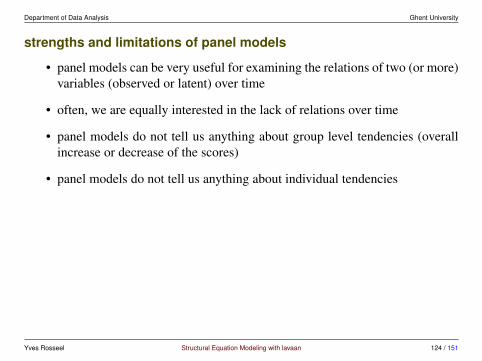
strengths and limitations of panel models
• panel models can be very useful for examining the relations of two (or more)variables (observed or latent) over time
• often, we are equally interested in the lack of relations over time
• panel models do not tell us anything about group level tendencies (overallincrease or decrease of the scores)
• panel models do not tell us anything about individual tendencies
Yves Rosseel Structural Equation Modeling with lavaan 124 / 151
Department of Data Analysis Ghent University
6.3 Growth curve models• ‘time’ is typically considered as a continuous variable
• two components:
– fixed effects: what is the nature of the average trend (linear, quadratic)– random effects: individual differences
• in addition, we may try to explain these individual differences by taking intoaccount:
– time-invariant covariates (age, gender, . . . )– time-varying covariates (measured at each time point)
• closely related to ‘mixed models’ (linear mixed models, generalized mixedmodels)
– limited to balanced data– but we can add indirect paths and latent variables
• focus on the mean structure (not the covariance structure)
Yves Rosseel Structural Equation Modeling with lavaan 125 / 151
Department of Data Analysis Ghent University
some references
• Bollen, K.A., & Curran, P.J. (2006). Latent curve models: A structuralequation perspective. John Wiley & Sons.
Yves Rosseel Structural Equation Modeling with lavaan 128 / 151
Department of Data Analysis Ghent University
7.2 The two-level SEM model with random intercepts• we assume two-level data with individuals (students) nested within clusters
(schools)
• in this framework, we decompose the total score of each variable into twoparts: a within part, and a between part (Cronbach & Webb, 1979):
yji = (yji − yj) + yj
yT = yW + yB
where j = 1, . . . , J is an index for the clusters, and i = 1, . . . , nj is anindex for the units within a cluster; yj is the cluster mean of cluster j
– both components are treated as unknown (latent) variables
– the two parts are orthogonal and additive; one of the parts can be zero
• the total covariance (at the population level) can be decomposed as
Cov(y) = ΣT = ΣW + ΣB
Yves Rosseel Structural Equation Modeling with lavaan 129 / 151
Department of Data Analysis Ghent University
7.3 Two-level SEM in lavaan• multilevel SEM development started around jan 2017
• implemented in lavaan (0.6-3):
– standard two-level ‘within-and-between’ approach
– continuous responses only, no missing data (for now)
– no random slopes (for now)
– using quasi-newton optimization by default
– em algorithm available using the option optim.method = "em"
• future plans: many, but don’t ask when it will be ready
– missing data, random slopes
– gllamm framework (but more user-friendly)
– case-wise likelihood approach
– more levels
Yves Rosseel Structural Equation Modeling with lavaan 130 / 151
Department of Data Analysis Ghent University
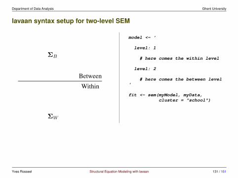
lavaan syntax setup for two-level SEM
ΣB
Between
Within
ΣW
model <- '
level: 1
# here comes the within level
level: 2
# here comes the between level'
fit <- sem(myModel, myData,cluster = "school")
Yves Rosseel Structural Equation Modeling with lavaan 131 / 151
Yves Rosseel Structural Equation Modeling with lavaan 147 / 151
Department of Data Analysis Ghent University
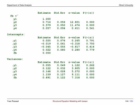
model 5: adding covariates (no output)
fb
y1 y2 y3 y4
w1
Between
Within
y1 y2 y3 y4
fw x1x2
model <- '
level: 1
fw =˜ y1 + y2 + y3 + y4fw ˜ x1 + x2
level: 2
fb =˜ y1 + y2 + y3 + y4fb ˜ w1
'
fit <- sem(model,data = Demo.twolevel,cluster = "cluster")
Yves Rosseel Structural Equation Modeling with lavaan 148 / 151
Department of Data Analysis Ghent University
7.4 Evaluating model fit• if no random slopes are involved, we can fit an unrestricted (saturated) model:
we estimate all the elements of ΣW , ΣB and µB
• then, we can compute the standard ‘χ2’ goodness-of-fit test statistic as:
T = −2(L0 − L1)
where L0 and L1 are the loglikelihood of the restricted (user-specified)model (h0) and the unrestricted model (h1) respectively
– under various optimal conditions, this statistic follows a chi-square dis-tribution
– the degrees of freedom are computed as in a two-group SEM model:the difference between the number of (non-redundant) sample statisticsfor each level, and the number of free model parameters
• in principle, fit measures like CFI/TLI, RMSEA, SRMR, . . . can be com-puted in a similar way as in a single-level SEM
Yves Rosseel Structural Equation Modeling with lavaan 149 / 151
Department of Data Analysis Ghent University
evaluating fit (2)
• unfortunately, a recent simulation study showed that CFI, TLI, and RMSEAwere not sensitive to Level-2 model misspecification:
Hsu, H.Y., Kwok, O.M., Lin, J.H., & Acosta, S. (2015). Detect-ing misspecified multilevel structural equation models with com-mon fit indices: a Monte Carlo study. Multivariate behavioralresearch, 50, 197–215.
• there seems to be a growing sentiment that ‘global’ fit indices may not bevery useful in a multilevel setting
• an alternative approach is to assess the fit per level:
– we could compute the SRMR for each level
– we could fit a model separately for each level, and leave the other levelsaturated
Yves Rosseel Structural Equation Modeling with lavaan 150 / 151
Department of Data Analysis Ghent University
Thank you for attending this workshop!
Yves Rosseel Structural Equation Modeling with lavaan 151 / 151