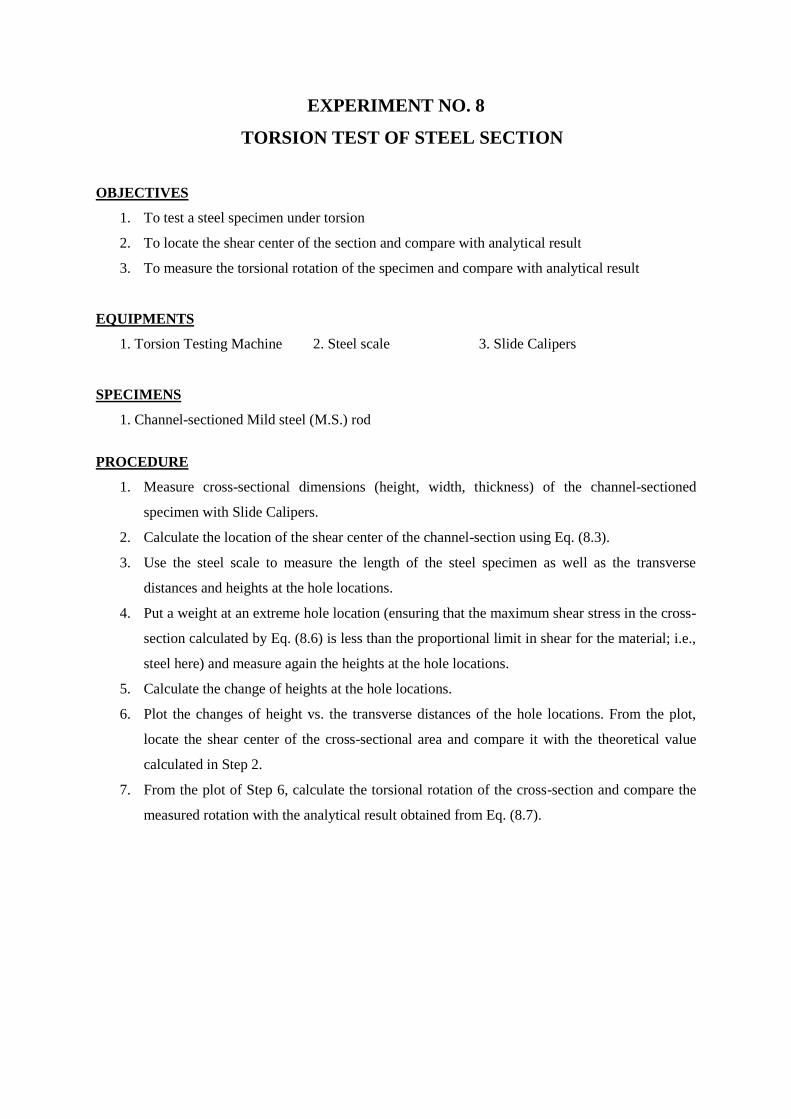
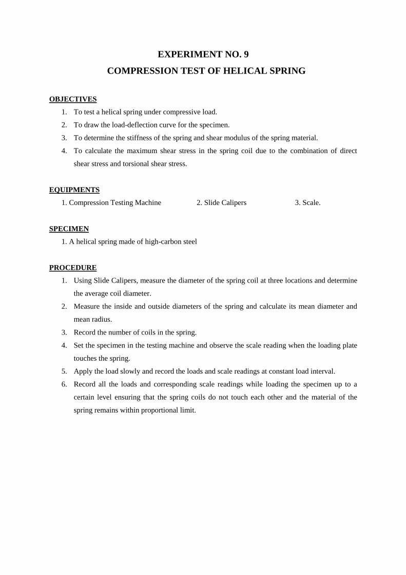
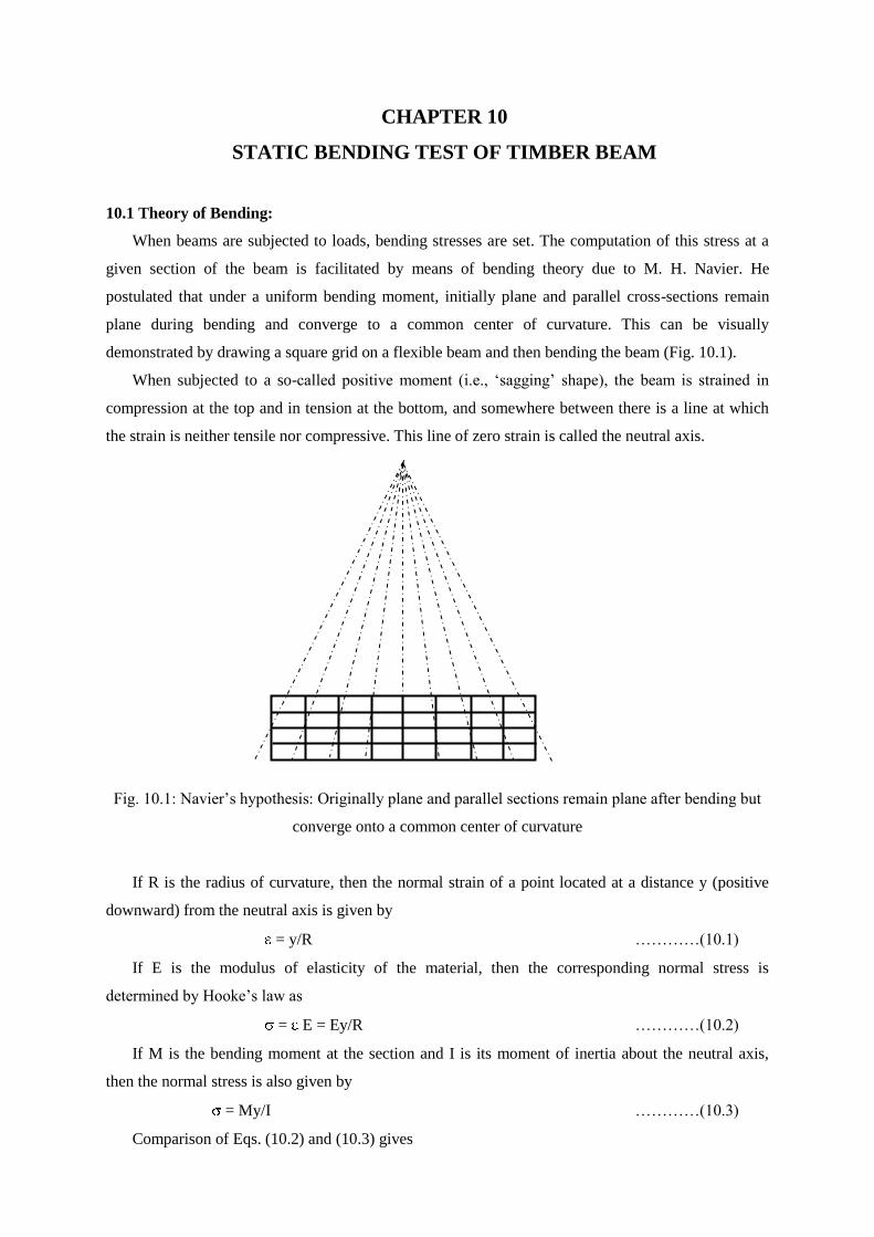
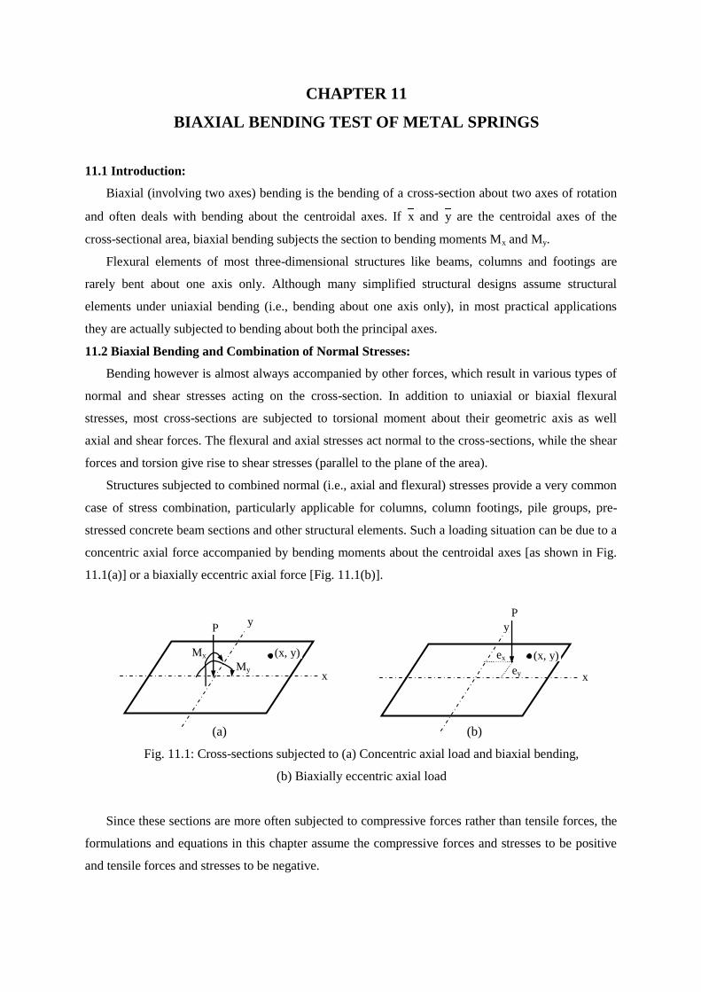
Page 1
CHAPTER 1
ENGINEERING MECHANICS I
1.1 Verification of Lame’s Theorem:
If three concurrent forces are in equilibrium, Lame’s theorem states that their magnitudes are
proportional to the sine of the angle between the other forces. For example, Fig. 1.1(a) shows three
concurrent forces P, Q and R in equilibrium, with the included angles between Q-R, R-P and P-Q
being , and respectively.
Therefore, Lame’s theorem states that
P/sin = Q/sin = R/sin ….………………..(1.1)
Since = 360 , sin = sin ( + ), and Eq. (1.1) becomes
P/sin = Q/sin = R/sin ( + ) ….………………..(1.2)
R D1 D2
P
F1 F2
W
Q
(a) (b)
Fig. 1.1: (a) Three concurrent forces in equilibrium, (b) Lab arrangement for Exp. 1.1
In the laboratory experiment, equilibrium is achieved among the forces F1, F2 and W. Lame’s
theorem F1/sin (180 2) = F2/sin (180 1) = W/sin ( 1+ 2)
F1 = W sin ( 2)/sin ( 1+ 2) …………..(1.3)
F2 = W sin ( 1)/sin ( 1+ 2) …………..(1.4)
The angles 1 and 2 are obtained from
1 = tan-1
(D1/L) …………..(1.5)
2 = tan-1
(D2/L) …………..(1.6)
1 2 L
Page 2
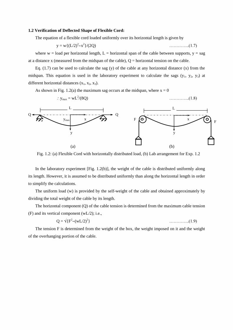
1.2 Verification of Deflected Shape of Flexible Cord:
The equation of a flexible cord loaded uniformly over its horizontal length is given by
y = w{(L/2)2
x2}/(2Q) …………..(1.7)
where w = load per horizontal length, L = horizontal span of the cable between supports, y = sag
at a distance x (measured from the midspan of the cable), Q = horizontal tension on the cable.
Eq. (1.7) can be used to calculate the sag (y) of the cable at any horizontal distance (x) from the
midspan. This equation is used in the laboratory experiment to calculate the sags (y1, y2, y3) at
different horizontal distances (x1, x2, x3).
As shown in Fig. 1.2(a) the maximum sag occurs at the midspan, where x = 0
ymax = wL2/(8Q) …………..(1.8)
Q Q
ymax x x
y y
(a) (b)
Fig. 1.2: (a) Flexible Cord with horizontally distributed load, (b) Lab arrangement for Exp. 1.2
In the laboratory experiment [Fig. 1.2(b)], the weight of the cable is distributed uniformly along
its length. However, it is assumed to be distributed uniformly than along the horizontal length in order
to simplify the calculations.
The uniform load (w) is provided by the self-weight of the cable and obtained approximately by
dividing the total weight of the cable by its length.
The horizontal component (Q) of the cable tension is determined from the maximum cable tension
(F) and its vertical component (wL/2); i.e.,
Q = {F2
(wL/2)2} …………..(1.9)
The tension F is determined from the weight of the box, the weight imposed on it and the weight
of the overhanging portion of the cable.
L L
F F
Page 3
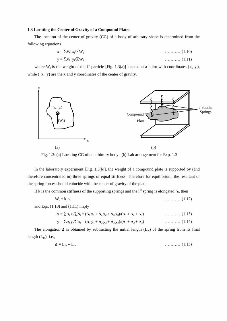
1.3 Locating the Center of Gravity of a Compound Plate:
The location of the center of gravity (CG) of a body of arbitrary shape is determined from the
following equations
x = Wi xi/ Wi …………(1.10)
y = Wi yi/ Wi …………(1.11)
where Wi is the weight of the ith particle [Fig. 1.3(a)] located at a point with coordinates (xi, yi),
while ( x, y) are the x and y coordinates of the center of gravity.
y
Compound
Plate
x
(a) (b)
Fig. 1.3: (a) Locating CG of an arbitrary body , (b) Lab arrangement for Exp. 1.3
In the laboratory experiment [Fig. 1.3(b)], the weight of a compound plate is supported by (and
therefore concentrated in) three springs of equal stiffness. Therefore for equilibrium, the resultant of
the spring forces should coincide with the center of gravity of the plate.
If k is the common stiffness of the supporting springs and the ith spring is elongated i, then
Wi = k i …………(1.12)
and Eqs. (1.10) and (1.11) imply
x = i xi/ i = ( 1 x1 + 2 x2 + 3 x3)/( 1 + 2 + 3) …………(1.13)
y = i yi/ I = ( 1 y1 + 2 y2 + 3 y3)/( 1 + 2 + 3) …………(1.14)
The elongation is obtained by subtracting the initial length (Lin) of the spring from its final
length (Lfn); i.e.,
= Lfn Lin …………(1.15)
(xi, yi)
(Wi)
3 Similar
Springs
Page 4
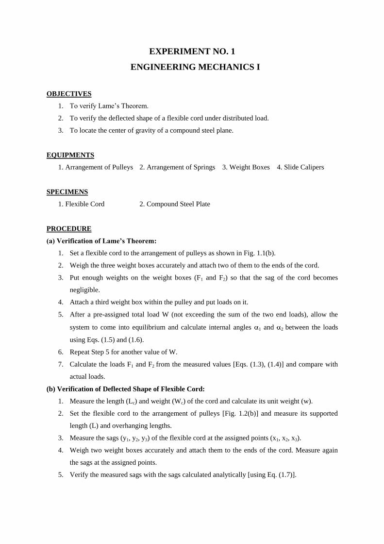
EXPERIMENT NO. 1
ENGINEERING MECHANICS I
OBJECTIVES
1. To verify Lame’s Theorem.
2. To verify the deflected shape of a flexible cord under distributed load.
3. To locate the center of gravity of a compound steel plane.
EQUIPMENTS
1. Arrangement of Pulleys 2. Arrangement of Springs 3. Weight Boxes 4. Slide Calipers
SPECIMENS
1. Flexible Cord 2. Compound Steel Plate
PROCEDURE
(a) Verification of Lame’s Theorem:
1. Set a flexible cord to the arrangement of pulleys as shown in Fig. 1.1(b).
2. Weigh the three weight boxes accurately and attach two of them to the ends of the cord.
3. Put enough weights on the weight boxes (F1 and F2) so that the sag of the cord becomes
negligible.
4. Attach a third weight box within the pulley and put loads on it.
5. After a pre-assigned total load W (not exceeding the sum of the two end loads), allow the
system to come into equilibrium and calculate internal angles 1 and 2 between the loads
using Eqs. (1.5) and (1.6).
6. Repeat Step 5 for another value of W.
7. Calculate the loads F1 and F2 from the measured values [Eqs. (1.3), (1.4)] and compare with
actual loads.
(b) Verification of Deflected Shape of Flexible Cord:
1. Measure the length (Lc) and weight (Wc) of the cord and calculate its unit weight (w).
2. Set the flexible cord to the arrangement of pulleys [Fig. 1.2(b)] and measure its supported
length (L) and overhanging lengths.
3. Measure the sags (y1, y2, y3) of the flexible cord at the assigned points (x1, x2, x3).
4. Weigh two weight boxes accurately and attach them to the ends of the cord. Measure again
the sags at the assigned points.
5. Verify the measured sags with the sags calculated analytically [using Eq. (1.7)].
Page 5
(c) Locating the Center of Gravity of a Compound Plate:
1. Measure accurately the dimensions and weight of the compound plate and determine the
location of its center of gravity analytically.
2. Measure the initial lengths (Lin) of the springs in the Spring Arrangement.
3. Attach the plate to the Spring Arrangement and determine the coordinates (x, y) of the springs
on the plate.
4. Measure the final lengths (Lfn) of the springs again and calculate the elongations ( ), using
Eq. (1.15).
5. Assume the forces in the springs are proportional to the elongations and thereby locate the
resultant of the forces [using Eqs. (1.13), (1.14)].
6. Compare the analytical center of gravity with its measured location.
Page 6
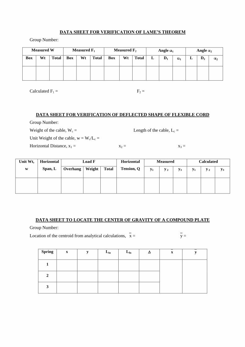
DATA SHEET FOR VERIFICATION OF LAME’S THEOREM
Group Number:
Measured W Measured F1 Measured F2 Angle 1 Angle 2
Box Wt Total Box Wt Total Box Wt Total L D1 1 L D2 2
Calculated F1 = F2 =
DATA SHEET FOR VERIFICATION OF DEFLECTED SHAPE OF FLEXIBLE CORD
Group Number:
Weight of the cable, Wc = Length of the cable, Lc =
Unit Weight of the cable, w = Wc/Lc =
Horizontal Distance, x1 = x2 = x3 =
Unit Wt,
w
Horizontal
Span, L
Load F Horizontal
Tension, Q
Measured Calculated
Overhang Weight Total y1 y 2 y3 y1 y 2 y3
DATA SHEET TO LOCATE THE CENTER OF GRAVITY OF A COMPOUND PLATE
Group Number:
Location of the centroid from analytical calculations, x = y =
Spring x y Lin Lfn x y
1
2
3
Page 7
CHAPTER 2
ENGINEERING MECHANICS II
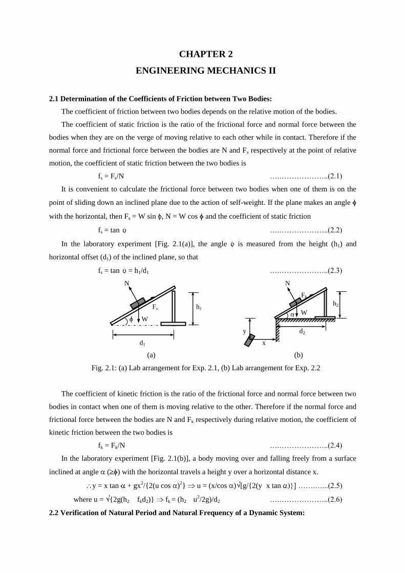
2.1 Determination of the Coefficients of Friction between Two Bodies:
The coefficient of friction between two bodies depends on the relative motion of the bodies.
The coefficient of static friction is the ratio of the frictional force and normal force between the
bodies when they are on the verge of moving relative to each other while in contact. Therefore if the
normal force and frictional force between the bodies are N and Fs respectively at the point of relative
motion, the coefficient of static friction between the two bodies is
fs = Fs/N ….………………..(2.1)
It is convenient to calculate the frictional force between two bodies when one of them is on the
point of sliding down an inclined plane due to the action of self-weight. If the plane makes an angle
with the horizontal, then Fs = W sin , N = W cos and the coefficient of static friction
fs = tan ….………………..(2.2)
In the laboratory experiment [Fig. 2.1(a)], the angle is measured from the height (h1) and
horizontal offset (d1) of the inclined plane, so that
fs = tan = h1/d1 ….………………..(2.3)
N N
Fk
Fs h1
W
y d2
d1 x
(a) (b)
Fig. 2.1: (a) Lab arrangement for Exp. 2.1, (b) Lab arrangement for Exp. 2.2
The coefficient of kinetic friction is the ratio of the frictional force and normal force between two
bodies in contact when one of them is moving relative to the other. Therefore if the normal force and
frictional force between the bodies are N and Fk respectively during relative motion, the coefficient of
kinetic friction between the two bodies is
fk = Fk/N ….………………..(2.4)
In the laboratory experiment [Fig. 2.1(b)], a body moving over and falling freely from a surface
inclined at angle ( ) with the horizontal travels a height y over a horizontal distance x.
y = x tan + gx2/{2(u cos )
2} u = (x/cos ) [g/{2(y x tan )}] …….…...(2.5)
where u = {2g(h2 fkd2)} fk = (h2 u2/2g)/d2 ….………………..(2.6)
2.2 Verification of Natural Period and Natural Frequency of a Dynamic System:
W h2
Page 8
A dynamic system may consist of a spring that provides stiffness, mass to provide inertia and
damping to reduce/stop its vibration. Stiffness (k) is the force required to produce unit displacement,
mass (m) represents the amount of matter and damping (c) is due to various mechanisms (like friction,
drag etc.) to resist motion.
When an undamped dynamic system undergoes free vibration (i.e., vibration without external
excitation), it follows the simple harmonic motion representing repetitive cycles of vibration of
similar amplitude and duration.
The natural period is the time taken by the system to complete one cycle of vibration.
Natural frequency is the opposite of natural period; i.e., it is the number of cycles completed by
the dynamic system in unit time (e.g., second). Although this definition is more convenient, natural
frequency in scientific terms is often multiplied by 2 , and its unit expressed in radian per second.
This definition of the natural frequency is given by the expression
n = (k/m) …………..(2.7)
In cycles per second (Hz), natural frequency is
fn = n/2 …………..(2.8)
The natural period is the inverse of the natural frequency in Hz; i.e.,
T = 1/fn …………..(2.9)
k
k
m
(a) (b)
Fig. 2.2: (a) Unstretched spring, (b) Mass m and stretched spring of stiffness k
In the laboratory experiment [Figs. 2.2(a) and 2.2(b)], a spring-mass system is attached to a mass
m [= weight W/g]. If the weight causes the spring to stretch by , the spring stiffness
k = W/ …………(2.10)
Therefore, Eq. (2.7) n = (k/m) = (W/ )/(W/g) = (g/ ) …………(2.11)
From the natural frequency calculated in Eq. (2.11), the natural period can be determined from
Eqs. (2.8) and (2.9).
Page 9
2.3 Determination of the Coefficient of Restitution and Use in the Equation of Projectile:
Coefficient of restitution is a measure of the amount of energy that can be recovered elastically
after the impact between two bodies. It is used often in impact problems and is the ratio of the relative
velocity of rebound between two bodies and their relative velocity of impact. If one of the bodies is at
rest (e.g., a ball hitting the floor slab or the wall), the coefficient is simply the ratio of the velocity of
rebound and velocity of impact of the moving body.
In the laboratory experiment [Fig. 2.3(a)], the coefficient of restitution is determined by dropping
a ball from a height h1 and calculating the height h2 it reaches after rebound from a fixed surface (i.e.,
the floor). Therefore, the impact velocity v1 = (2gh1), rebound velocity v2 = (2gh2) and the
coefficient of restitution,
e = v2/v1 = (h2/h1) …………(2.12)
Along the same line
h1
h2 y1
v2 v3
x1 x2
(a) (b)
Fig. 2.3: (a) Determining e, (b) Lab arrangement for Exp. 2.3
In the laboratory experiment [Fig. 2.3(b)], a ball is delivered from a height y1 with a velocity v1 at
an angle with the horizontal, hits the ground at a distance x1 with a velocity v2 (angled with
horizontal), rebounds with a velocity v3 (at an angle with horizontal) and reaches a height y2 at a
horizontal distance x2 from the point of impact. The ball will follow the path of a projectile
throughout, while the relationship between v2 and v3 will depend on the coefficient of restitution. The
equations of motion are given by y1 = x1 tan + g (x1/v1 cos )2/2; v2 sin = {(v1 sin )
2 + 2gy1}; v3
sin = e v2 sin ; v3 cos = v2 cos = v1 cos and y2 = x2 tan g (x2/v3 cos )2/2.
If the velocity v1, height y1, distance x1 and coefficient e are known, the angle and height y2 can
be calculated by the equations shown above. However if the distances are small and velocity of
release is quite large, the effect of gravity can be ignored so the equations are approximated to
tan y1/x 1 …………(2.13)
y2 e x2 tan e y1 (x2 /x1) …………(2.14)
y2
v1
Page 10
EXPERIMENT NO. 2
ENGINEERING MECHANICS II
OBJECTIVES
1. To determine the coefficient of static and kinetic friction between two bodies.
2. To verify the natural period and natural frequency of a dynamic system.
3. To determine the coefficient of restitution and use in the equation of a projectile.
EQUIPMENTS
1. Inclined Plane System 2. Dynamic system 3. Steel Scale 4. Tape 5. Watch
SPECIMENS
1. Timber Block 2. Tennis Ball 3. Rubber Ball
PROCEDURE
(a) Determination of the Coefficients of Friction between Two Bodies:
Static Friction
1. Set the plane system horizontally and put the timber block on the plane.
2. Gradually increase the angle of inclination of the plane with the horizontal until the timber
block slides down the plane.
3. Measure the height h1 and horizontal offset d1 of the inclined plane when the timber block is
on the point of sliding down and calculate the angle of the plane with the horizontal using Eq.
(2.3). This gives the angle of static friction ( ) between the plane and the timber block while
the tangent of this angle is the corresponding coefficient of static friction (fs).
Kinetic Friction
1. Set the plane system at an angle , which is greater than its angle of static friction . Put the
system at an elevated position and measure the height h2 and horizontal offset d2 of the
inclined plane to calculate the angle .
2. Put the timber block on the plane and allow it to slide down the plane.
3. Allow the block to leave the plane and drop to the ground. Measure the height (y) it falls from
and the horizontal distance (x) it travels. Use Eq. (2.5) to calculate the velocity (u) while
leaving the inclined plane and Eq. (2.6) to calculate the corresponding coefficient of kinetic
friction (fk).
Page 11
(b) Verification of Natural Period and Natural Frequency of a Dynamic System:
1. Measure the weight (W) of the dynamic system and the free length of its spring.
2. Suspend the weight from the end of the spring, measure the elongation ( ) and calculate its
stiffness (k) using Eq. (2.10) and natural frequency using Eq. (2.11)
3. Calculate the corresponding natural period of the system using Eqs. (2.8) and (2.9).
4. Suspend the weight from the spring and let it vibrate freely. Allow about 15-20 vibrations and
measure the natural period of the system. Also calculate the natural frequency of the system.
5. Verify the measured natural period and frequency with the ones calculated analytically.
6. Repeat the process (Steps 1 to 5) by increasing the weight of the system.
(c) Determination of the Coefficient of Restitution and Use in the Equation of Projectile:
1. Drop a tennis/rubber ball (projectile) from a height h1 measured initially and measure the
height h2 it rebounds to. Use Eq. (2.12) to calculate the coefficient of restitution, e.
2. Mark the projectile so that its impact points can be located easily.
3. Measure the height y1 from which the projectile is released.
4. Release the projectile at a reasonably high speed and mark the points it reaches on the floor
(distance x1) and wall (height y2). Also measure the horizontal distance x2.
5. Calculate y2 approximately from Eq. (2.14) using the measured values of e, x1, x2 and y1 and
compare with the measured value of y2.
Page 12
DATA SHEET FOR DETERMINATION OF COEFFICIENTS OF FRICTION
Group Number:
Static Friction Kinetic Friction
Height,
h1
Offset,
d1
Friction
Factor,
fs
Angle of
Friction,
Height,
h2
Offset,
d2
Angle,
x y Velocity, u Friction
Factor,
fk
…. ....
DATA SHEET FOR VERIFICATION OF NATURAL PERIOD AND FREQUENCY
Group Number:
Spring
Elongation,
Calculated Values Measurements
Natural
Frequency
Natural
Period
No. of
Cycles
Time Natural
Frequency
Natural
Period
DATA SHEET FOR DETERMINATION OF COEFFICIENT OF RESTITUTION AND
USE FOR PROJECTILE
Group Number:
Coefficient of Restitution Measured Values Calculated
y2 Ht, h1 Ht, h2 Coeff, e Dist, x1 Dist, x2 Ht, y1 Ht, y2
Page 13
CHAPTER 3
TENSION TEST OF MILD STEEL
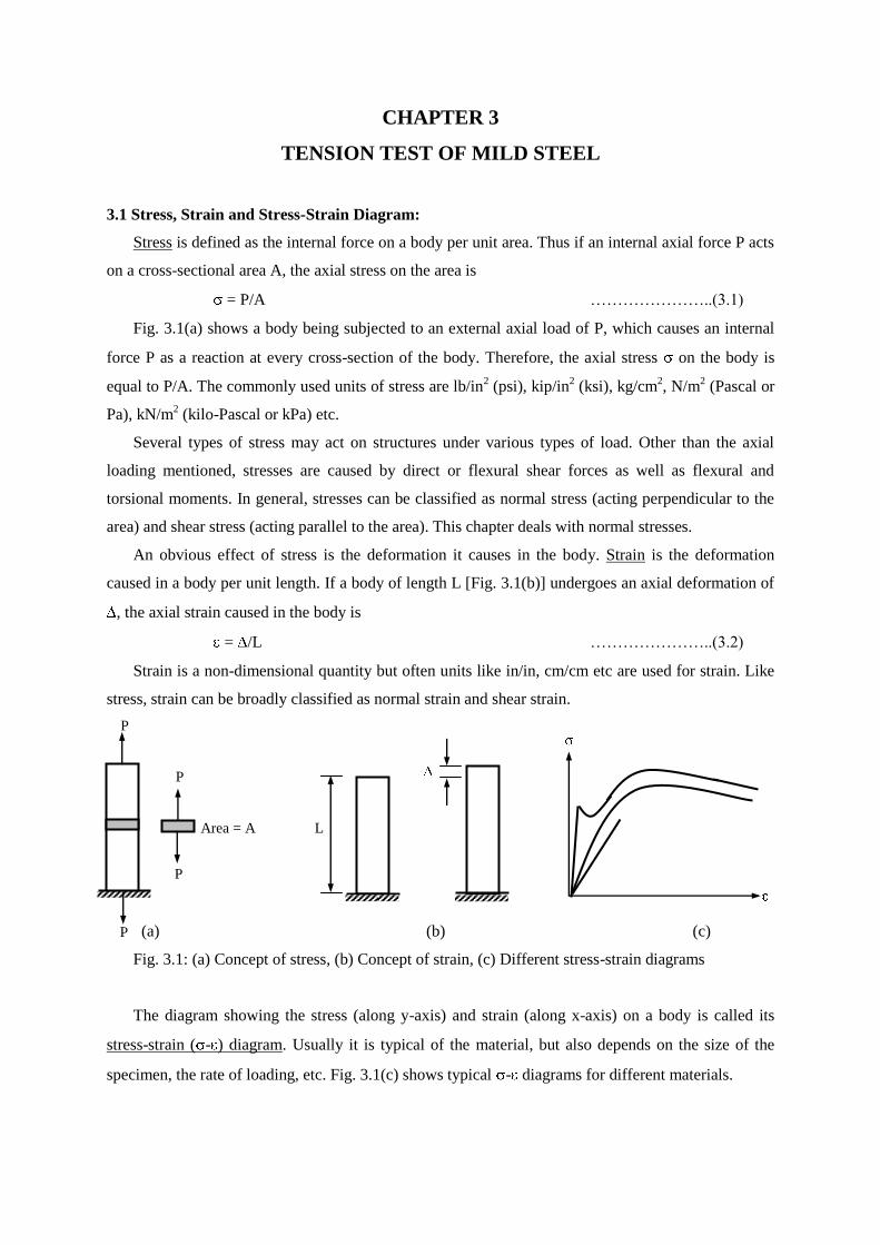
3.1 Stress, Strain and Stress-Strain Diagram:
Stress is defined as the internal force on a body per unit area. Thus if an internal axial force P acts
on a cross-sectional area A, the axial stress on the area is
= P/A …………………..(3.1)
Fig. 3.1(a) shows a body being subjected to an external axial load of P, which causes an internal
force P as a reaction at every cross-section of the body. Therefore, the axial stress on the body is
equal to P/A. The commonly used units of stress are lb/in2 (psi), kip/in
2 (ksi), kg/cm
2, N/m
2 (Pascal or
Pa), kN/m2 (kilo-Pascal or kPa) etc.
Several types of stress may act on structures under various types of load. Other than the axial
loading mentioned, stresses are caused by direct or flexural shear forces as well as flexural and
torsional moments. In general, stresses can be classified as normal stress (acting perpendicular to the
area) and shear stress (acting parallel to the area). This chapter deals with normal stresses.
An obvious effect of stress is the deformation it causes in the body. Strain is the deformation
caused in a body per unit length. If a body of length L [Fig. 3.1(b)] undergoes an axial deformation of
, the axial strain caused in the body is
= /L …………………..(3.2)
Strain is a non-dimensional quantity but often units like in/in, cm/cm etc are used for strain. Like
stress, strain can be broadly classified as normal strain and shear strain.
Area = A L
(a) (b) (c)
Fig. 3.1: (a) Concept of stress, (b) Concept of strain, (c) Different stress-strain diagrams
The diagram showing the stress (along y-axis) and strain (along x-axis) on a body is called its
stress-strain ( - ) diagram. Usually it is typical of the material, but also depends on the size of the
specimen, the rate of loading, etc. Fig. 3.1(c) shows typical - diagrams for different materials.
P
P
P
P
Page 14
3.2 Definition of Essential Terms in the Stress-Strain Diagram:
The stress vs. strain ( - ) diagrams discussed in the previous section are often used in studying
various mechanical properties of materials under the action of loads. Depending on the type of
materials, the - diagrams are drawn for specimens subjected to tension (typically for mild steel,
aluminum and several other metals, less often for granular materials) or compression (more often for
concrete, timber, soil and other granular materials).
Several elements of the - diagrams are used in Strength of Materials as well as structural
analysis and design. Figs. 3.2 (a) and 3.2 (b) show two typical stress-strain diagrams often
encountered in material testing. The first of them represents a material with an initial linear -
relationship followed by a pronounced yield region, which is often followed by a strain hardening and
failure region. This is typical of relatively lower-strength steel. The second curve represents a material
with nonlinear - relationship almost from the beginning and no distinct yield region. The -
diagram of high-strength steel or timber, which is studied subsequently, represents such a material.
(a) (b)
Fig. 3.2: Typical stress-strain diagrams for (a) Yielding materials, (b) Non-yielding materials
Up to a certain limit of stress and strain, the - diagram for most materials remain linear (or
nearly so); i.e., the stress remains proportional to the strain initially. Up to this limit, the material
follows the Hooke’s Law, which states that deformation is proportional to applied load. The
corresponding stress is called the proportional limit (or elastic limit), which is denoted by p in Fig.
3.2(a), and the strain is denoted by p. The ratio of p and p (or any stress and strain below these) is
called the Modulus of Elasticity or Young’s Modulus and is denoted by E.
E = p/ p …………………..(3.3)
The area under the - diagram indicates the energy dissipated per unit volume in straining the
material under study. The corresponding area up to the proportional limit is called Modulus of
Resilience and is given by the following equation
Modulus of Resilience = p p/2 = p2/2E …………………..(3.4)
p
p
yu
yl
ult
brk
y(offset) y(proof)
y(offset) y(proof)
Apparent - Curve
Actual - Curve
Page 15
Longitudinal strain is accompanied by lateral strain as well, of different magnitude and opposite
sign. If the longitudinal strain is long and the corresponding lateral strain is lat, the ratio between the
two is called the Poisson’s Ratio, often denoted by .
= lat/ lomg …………………..(3.5)
The Modulus of Elasticity and the Poisson’s Ratio are two basic material constants used
universally for the linear elastic analysis and design.
Within proportional limit, the - diagram passes through the origin. Therefore, the strain
sustained within the proportional limit can be fully recovered upon withdrawal of the load; i.e.,
without any permanent deformation of the material. However, this is not applicable if the material is
stressed beyond p. If load is withdrawn after stressing the material beyond yield point, the -
diagram follows the initial straight path during the process of unloading and therefore does not pass
through the origin; i.e., the strain does not return to zero even when stress becomes zero.
In many materials, the proportional limit is followed by a stress (or small range of stresses) where
the material is elongated (i.e., strained) without any significant change in stress. This is called the
yield strength for the material and is often denoted by y. As shown in Fig. 3.2 (a), yielding occurs
within a range of stress rather than any particular stress. The upper limit of the region is called upper
yield strength while the lower limit is called lower yield strength of the material. In Fig. 3.2 (a), they
are denoted by yu and yl respectively.
However materials with - diagrams similar to Fig. 3.2 (b) do not have any particular yield point
or region. In order to indicate the stress where the material is strained within the range of typical yield
strains or undergoes permanent deformation typical of yield points, two methods have been suggested
to locate the ‘yield point’ of non-yielding materials. One of the is the Proof Strength, which takes the
stress y(proof) as the yield point of the material corresponding to a pre-assigned strain indicated by
y(proof). The other is the Offset Method, which takes as yield point a point corresponding to a
permanent strain of y(offset). Therefore the yield strength by Offset Method is obtained by drawing a
straight line from y(offset) parallel to the initial tangent of the - diagram and taking as yield strength
the point where this line intersects the - diagram.
Beyond yield point, the strains increase at a much faster rate with nominal increase in stress and
the material moves towards failure. However, the material can usually take stresses higher than its
yield strength. The maximum stress a material can sustain without failure is called the ultimate
strength, which is denoted by ult in Fig. 3.2 (a). For most materials, the stress decreases as the
material is strained beyond ult until failure occurs at a stress called breaking strength of the material,
denoted by brk in Fig. 3.2 (a).
Here it may be mentioned that the stress does not actually decrease beyond ultimate strength in
the true sense. If the actual - diagram [indicated by dotted lines in Fig. 3.2 (a)] of the material is
drawn using the instantaneous area (which is smaller than the actual area due to Poisson’s effect) and
length of the specimen instead of the original area and length, the stress will keep increasing until
Page 16
failure. All the other - diagrams shown in Figs. 3.1 and 3.2 (and used for most Civil Engineering
applications) are therefore called apparent - diagrams.
The total area under the - diagram is called the Modulus of Toughness. Physically, this is
energy required to break a specimen of unit volume.
Ductility is another property of vital importance to structural design. This is the ability of the
material to sustain strain beyond elastic limit. Quantitatively it is taken as the final strain in the
material (the strain at failure) expressed in percentage.
Table 3.1 shows some useful mechanical properties of typical engineering materials. Here it may
be mentioned that these properties may vary significantly depending on the ingredients used and the
manufacturing process. For example, although the yield strength of Mild Steel is shown to be 40 ksi,
other varieties with yield strengths of 60 ksi and 75 ksi are readily available. The properties of
concrete are even more unpredictable. Here, the ultimate strength is mentioned to be 3 ksi, but
concretes with much lower and higher ultimate strengths (1~7 ksi) are used in different construction
works. The values mentioned in the table are quoted from available literature.
Table 3.1: Useful Mechanical Properties of Typical Engineering Materials
Material p
(ksi)
y
(ksi)
ult
(ksi)
E
(ksi)
Modulus of
Resilience
(ksi)
Modulus of
Toughness
(ksi)
Ductility
(%)
Reduction
of Area
(%)
Mild Steel 35 40 60 29000 0.25 0.02 15 35 60
Aluminum
Alloy 60 70 80 10000 0.33 0.18 7 10 30
Alloy Steel 210 215 230 29000 0.30 0.73 20 10 20
Concrete 1.4 2.0 3.0 3000 0.30 0.0004 0.006 0.30 0.60
[Note: Properties may vary significantly depending on ingredients and manufacturing process]
3.3 The Standard Tension Test of Mild Steel:
The tension test of mild steel has been standardized by ASTM. The specimens to be used are
almost always cylindrical or prismatic, with substantially constant cross-sectional area for uniformity
of stress. The ends are usually enlarged for added strength so that rupture does not take place near the
grips. Since abrupt changes in cross-sections cause stress concentrations, the transition from central
portion to the larger ends is made by fillet of large radius.
The experimental measurements are made on the central reduced portion, commonly 0.5 inch in
diameter and 2.25 inches long, which allows the use of a 2-inch gage length. It is often tapered very
slightly (0.003-0.005 inch) toward the center to ensure rupture near the middle. The ends are 0.75 inch
diameter and threaded to screw the specimen holders on the testing machine.
Page 17
2
1.375 2.25 1.375
Fig. 3.3: ASTM mild steel specimen for tension test
During the test, loads are applied by hydraulic machine while elongations are measured at
different stages by a combination of extensometer and divider. The gage length of the specimen is
fixed by punching gage marks on the surface of the specimen so that large changes in the length can
be measured by dividers.
After aligning the specimen properly in the testing machine and attaching an appropriate
extensometer within the gage length, load is applied slowly in order to avoid dynamic effects and
ensure that the specimen is in equilibrium at all stages.
Particular loads like yield point, ultimate load and breaking load are recorded during the progress
of the experiment. If it is carried up to rupture, the final elongation and cross-sectional area can also
be measured.
The character of the failure surface is often a revealing piece of information and should be
described. For mild steel, the typical cup-cone failure surface indicates a shear slippage (at yield)
followed by tensile failure (at rupture).
3.4 Mechanical Properties of Mild Steel:
Mild steel is one of the most important and widely used structural materials all over the world. Its
use as a construction material is of great importance to Civil Engineers, particularly for steel and
reinforced concrete structures (where steel is used to provide the tension carrying capacity of
concrete). Therefore the tension test of mild steel is very important from a structural designer’s point
of view and it is one of the commonly used material tests in Strength of Materials. The tensile strength
and elastic properties of mild steel obtained from this test are used in buildings, bridges, towers,
trusses, poles, water tanks and various other structural applications.
Some typical mechanical properties of mild steel, already mentioned in Table 3.1, are repeated
here in view of their importance in structural design and in the context of the current experiment.
These properties are as follows
Proportional Limit, p = 30~65 ksi (larger for stronger specimens)
Yield Strength, y = 35~75 ksi (larger for stronger specimens)
Ultimate Strength, ult = 60~100 ksi (larger for stronger specimens)
Modulus of Elasticity, E = 29000~30000 ksi (almost uniform for all types of specimens)
0.75 0.50
Page 18
Poisson’s Ratio, E = 0.20~0.30 ksi (larger for stronger specimens)
Modulus of Resilience = 0.02~0.07 ksi (larger for stronger specimens)
Modulus of Toughness = 7~15 ksi (smaller for stronger specimens)
Ductility = 10~35% (smaller for stronger specimens)
Reduction of Area = 20~60% (smaller for stronger specimens)
As shown above, these properties may vary significantly depending on the ingredients and
manufacturing process.
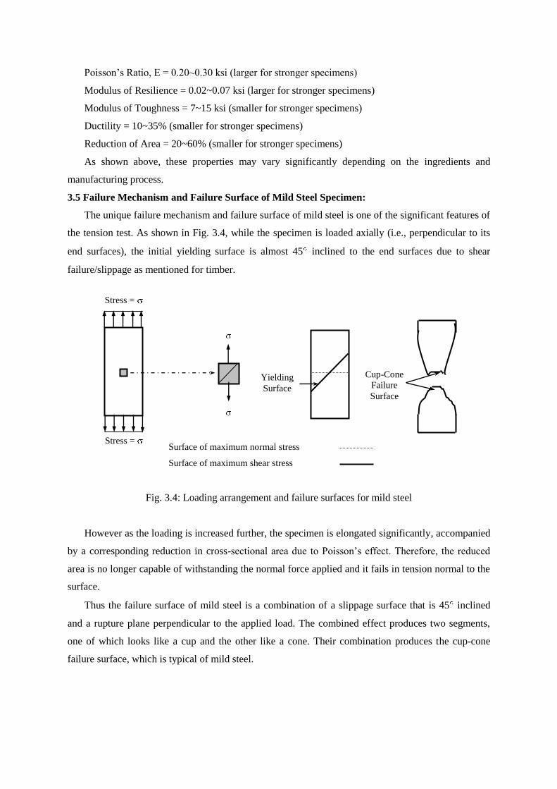
3.5 Failure Mechanism and Failure Surface of Mild Steel Specimen:
The unique failure mechanism and failure surface of mild steel is one of the significant features of
the tension test. As shown in Fig. 3.4, while the specimen is loaded axially (i.e., perpendicular to its
end surfaces), the initial yielding surface is almost 45 inclined to the end surfaces due to shear
failure/slippage as mentioned for timber.
Surface of maximum normal stress
Surface of maximum shear stress
Fig. 3.4: Loading arrangement and failure surfaces for mild steel
However as the loading is increased further, the specimen is elongated significantly, accompanied
by a corresponding reduction in cross-sectional area due to Poisson’s effect. Therefore, the reduced
area is no longer capable of withstanding the normal force applied and it fails in tension normal to the
surface.
Thus the failure surface of mild steel is a combination of a slippage surface that is 45 inclined
and a rupture plane perpendicular to the applied load. The combined effect produces two segments,
one of which looks like a cup and the other like a cone. Their combination produces the cup-cone
failure surface, which is typical of mild steel.
Stress =
Yielding
Surface
Cup-Cone
Failure
Surface
Stress =
Page 19
EXPERIMENT NO. 3
TENSION TEST OF MILD STEEL
OBJECTIVES
1. To test a mild steel specimen to failure under tensile load.
2. To draw the stress-strain curve.
3. To determine the proportional limit, modulus of elasticity, modulus of resilience, yield
strength, ultimate strength and elongation percentage from the stress-strain curve.
4. To observe the failure surface.
EQUIPMENTS
1. Universal Testing Machine 2. Extensometer 3. Slide Calipers
SPECIMEN
1. Mild Steel rod.
PROCEDURE
1. Measure the diameter of the specimen at several points and calculate its mean diameter.
2. Record the gage length of the specimen and the extensometer constant.
3. Set the machine to grip the specimen between its gage marks and attach the extensometer
suitably with the machine or the specimen to read the elongations. Adjust the extensometer
dial to read zero at this stage.
4. Apply the load slowly and record the loads and extensometer readings at constant load
interval.
5. Stop loading when the yield point is reached. Elongations beyond the yield point should be
recorded by an elongation scale attached to the machine.
6. Resume loading and take readings from the elongation scale at regular intervals until the
failure of the specimen.
7. Record the final (ultimate) load at failure and measure the final length between the gage
marks.
8. Note the characteristics of the failure surface.
Page 20
DATA SHEET FOR TENSION TEST OF MILD STEEL
Group Number:
Gage Length = Cross-sectional Area of the Specimen =
Obs.
No.
Readings from Load
Elongation
Stress
Strain
Remarks
Load Dial Extensometer
1
2
3
4
5
6
7
8
9
10
11
12
13
14
15
16
17
18
19
20
21
22
23
24
Calculate the following from the stress-strain diagram
1. Proportional Limit
2. Modulus of Elasticity
3. Modulus of Resilience
4. (a) Upper Yield Strength (b) Lower Yield Strength
5. Ultimate Strength
6. Elongation Percentage
Page 21
CHAPTER 4
COMPRESSION TEST OF TIMBER
4.1 Introduction:
Some basic concepts necessary for this experiment have already been discussed in Chapter 3.
These include stress ( ), strain ( ), stress-strain ( - ) diagram and the essential terms of the -
diagram; e.g., proportional limit (or elastic limit), modulus of elasticity or Young’s modulus,
modulus of resilience, yield strength by offset method, proof strength, ultimate strength, breaking
strength, modulus of toughness, ductility.
4.2 Mechanical Properties of Timber:
Since timber is a natural product, it is liable to a wide variation in strength and stiffness from one
variety to another. For structural purposes, timber is used as beams, columns, bracing elements and
piles. Teak, Gurjan, Jarul, Gamari, Sal etc. are among the more commonly used timbers available in
Bangladesh.
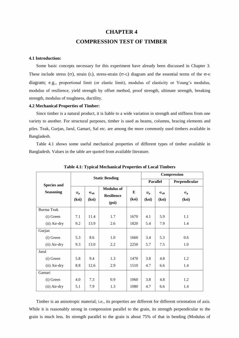
Table 4.1 shows some useful mechanical properties of different types of timber available in
Bangladesh. Values in the table are quoted from available literature.
Table 4.1: Typical Mechanical Properties of Local Timbers
Species and
Seasoning
Static Bending Compression
Parallel Perpendicular
p
(ksi)
ult
(ksi)
Modulus of
Resilience
(psi)
E
(ksi)
p
(ksi)
ult
(ksi)
p
(ksi)
Burma Teak
(i) Green
(ii) Air-dry
7.1
9.2
11.4
13.9
1.7
2.6
1670
1820
4.1
5.4
5.9
7.9
1.1
1.4
Gurjan
(i) Green
(ii) Air-dry
5.3
9.3
8.6
13.0
1.0
2.2
1660
2250
3.4
5.7
5.3
7.5
0.6
1.0
Jarul
(i) Green
(ii) Air-dry
5.8
8.8
9.4
12.6
1.3
2.9
1470
1510
3.8
4.7
4.8
6.6
1.2
1.4
Gamari
(i) Green
(ii) Air-dry
4.0
5.1
7.3
7.9
0.9
1.3
1060
1080
3.8
4.7
4.8
6.6
1.2
1.4
Timber is an anisotropic material; i.e., its properties are different for different orientation of axis.
While it is reasonably strong in compression parallel to the grain, its strength perpendicular to the
grain is much less. Its strength parallel to the grain is about 75% of that in bending (Modulus of
Page 22
Rupture), while for loading perpendicular to the grain and in shear its strength is only about 20% and
5% of its strength in bending. Timber has its greatest usable strength in tension and bending and is
slightly stronger in tension than in compression. The biggest advantage of timber as a structural
member is its light weight compared to the load it can sustain.
As the stress-strain diagram of timber has no specific yield point, its yield strength is determined
from the Offset Method and/or the Proof Strength Method. In the lab experiment, corresponding
strains being y (offset) = 0.0005 and y (proof) = 0.005 respectively.
4.3 Failure Mechanism and Failure Surface of Timber Specimen:
In addition to the - diagram and determination of the mechanical properties, another significant
feature of the compression test of timber is its failure surface. As shown in Fig. 4.1, while the
specimen is loaded axially (i.e., perpendicular to its end surfaces), the failure surface is observed to be
almost 45 inclined to the end surfaces.
Stress =
Stress = Surface of maximum normal stress
Surface of maximum shear stress
Fig. 4.1: Loading arrangement and surfaces of maximum stress
Fig. 4.1 shows the loading arrangement and surfaces of maximum normal stress and shearing
stress. Using the principles of stress transformation, it can be shown that the maximum normal stress
for such loadings is equal to the applied load ( ), at a surface perpendicular to the loading direction
while the maximum shearing stress is half that value ( /2), at an angle 45 inclined. Even then, the
timber specimen fails along the latter surface because of its relative weakness in shear compared to
axial stress, as discussed in the previous section.
Failure
Surface
Page 23
EXPERIMENT NO. 4
COMPRESSION TEST OF TIMBER
OBJECTIVES
1. To test a timber specimen under compressive load parallel to grain.
2. To draw the stress-strain curve of the specimen.
3. To determine the proportional limit, modulus of elasticity, modulus of resilience, yield
strength and ultimate strength of the specimen.
4. To compare the yield strength obtained by offset method with the proof strength.
5. To observe the failure surface.
EQUIPMENTS
1. Compression Testing Machine 2. Compressometer 3. Slide Calipers
SPECIMENS
1. Timber block of approximately (2 2 ) cross-section and 8 height.
PROCEDURE
1. Measure the dimensions of the specimen.
2. Record the gage length of the specimen and the compressometer constant.
3. Set the specimen in the testing machine and attach the compressometer suitably with the
machine or the specimen to read the deformations.
4. Set the machine so that the loading plates just touch the specimen and adjust the
compressometer dial to read zero at this stage.
5. Apply the load slowly and record the loads and compressometer readings at constant load
intervals until the failure of the specimen.
6. Record the final (ultimate) load at failure and measure the final length between the gage
marks.
7. Note the characteristics of the failure surface.
Page 24
DATA SHEET FOR COMPRESSION TEST OF TIMBER
Group Number:
Gage Length = Cross-sectional Area of the Specimen =
Obs.
No.
Readings from Load
Deformation
Stress
Strain
Remarks
Load Dial Compressometer
1
2
3
4
5
6
7
8
9
10
11
12
13
14
15
16
17
18
19
20
21
22
23
24
Calculate the following from the stress-strain diagram
1. Proportional Limit
2. Modulus of Elasticity
3. Modulus of Resilience
4. Yield strength from Offset Method
5. Proof strength
6. Ultimate strength
Page 25
CHAPTER 5
DIRECT SHEAR TEST OF METALS
5.1 Shearing Stress in Structural Members:
Shearing stress is one that acts parallel to a plane, unlike the tensile and compressive forces that
act normal to it. Shear stresses can be produced in structural bodies by various types of loading, such
as
1. Direct shear: If the resultants of parallel but opposite forces act through the centroid of the
sections that are spaced infinitesimal distances apart, the shearing stresses over the sections
are uniform. These stress conditions are called direct shear stress. Therefore, a shear force V
acting on a surface area A causes an average direct shear stress given by
= V/A …………………...(5.1)
Since the concept of infinitesimal distance is only theoretical, such conditions are never
completely realized in practical situations. However direct shear situations exist
approximately in rivets or welds connecting plates that are subjected to normal forces [Fig.
4.1(a), (b)]. For example, connections among truss members, beams and columns are often
subjected approximately to direct shear stresses. Direct shear situations are also approached in
laboratory tests by shearing forces distributed over very small lengths.
(a) (b)
Fig. 5.1: Direct shear in (a) rivet, (b) weld
Fig. 5.2: Flexural shear in rectangular beam
2. Flexural shear: Shear forces acting on sections as a result of differences in bending moments
are called flexural shear forces and the resulting stresses are called flexural shear stress.
Unlike direct shear stresses, these stresses are accompanied by substantial flexural stresses.
Also the flexural shear stresses are not uniformly distributed over the cross-sections, but are
instead zero at the top and bottom and reach the maximum value in between. For example, the
variation of flexural shear stress over a rectangular section is parabolic and the maximum
value reached at the middle of the section is 1.5 times the average shear stress [Fig. 5.2].
Parabolic variation of shear stress
Page 26
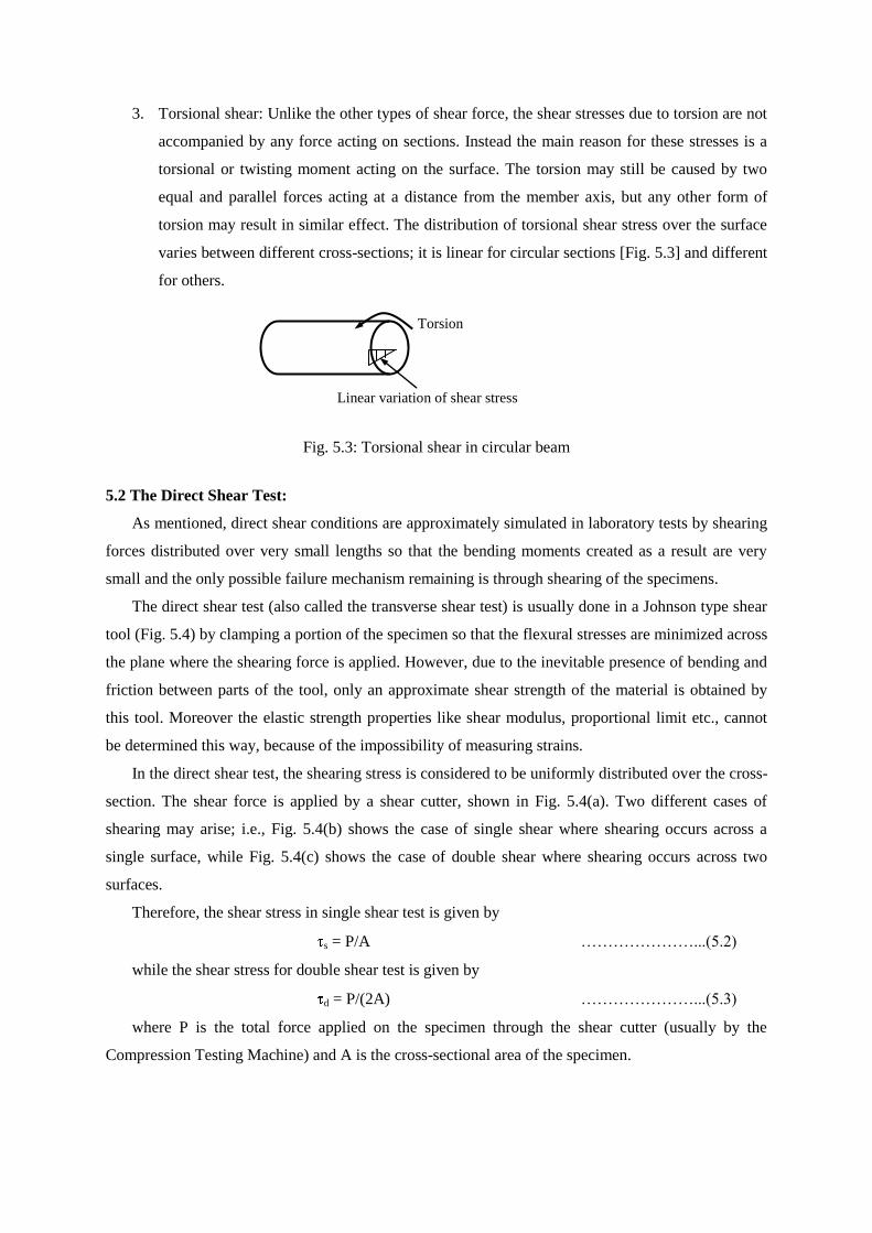
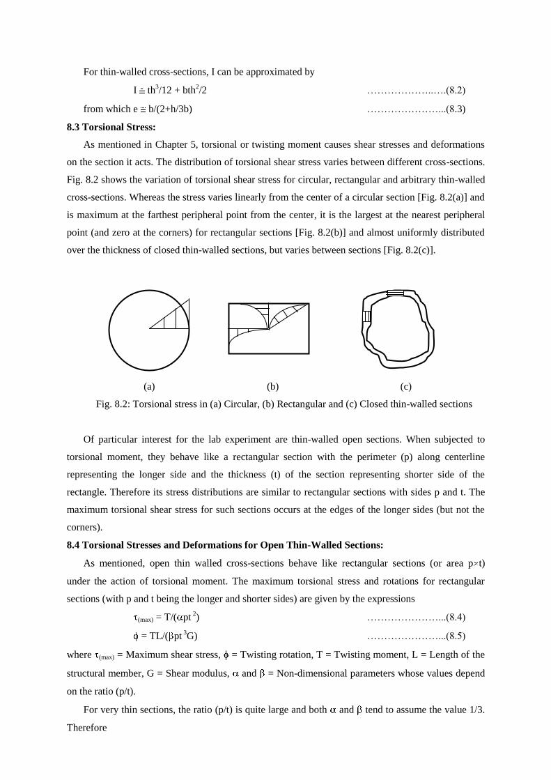
3. Torsional shear: Unlike the other types of shear force, the shear stresses due to torsion are not
accompanied by any force acting on sections. Instead the main reason for these stresses is a
torsional or twisting moment acting on the surface. The torsion may still be caused by two
equal and parallel forces acting at a distance from the member axis, but any other form of
torsion may result in similar effect. The distribution of torsional shear stress over the surface
varies between different cross-sections; it is linear for circular sections [Fig. 5.3] and different
for others.
Fig. 5.3: Torsional shear in circular beam
5.2 The Direct Shear Test:
As mentioned, direct shear conditions are approximately simulated in laboratory tests by shearing
forces distributed over very small lengths so that the bending moments created as a result are very
small and the only possible failure mechanism remaining is through shearing of the specimens.
The direct shear test (also called the transverse shear test) is usually done in a Johnson type shear
tool (Fig. 5.4) by clamping a portion of the specimen so that the flexural stresses are minimized across
the plane where the shearing force is applied. However, due to the inevitable presence of bending and
friction between parts of the tool, only an approximate shear strength of the material is obtained by
this tool. Moreover the elastic strength properties like shear modulus, proportional limit etc., cannot
be determined this way, because of the impossibility of measuring strains.
In the direct shear test, the shearing stress is considered to be uniformly distributed over the cross-
section. The shear force is applied by a shear cutter, shown in Fig. 5.4(a). Two different cases of
shearing may arise; i.e., Fig. 5.4(b) shows the case of single shear where shearing occurs across a
single surface, while Fig. 5.4(c) shows the case of double shear where shearing occurs across two
surfaces.
Therefore, the shear stress in single shear test is given by
s = P/A …………………...(5.2)
while the shear stress for double shear test is given by
d = P/(2A) …………………...(5.3)
where P is the total force applied on the specimen through the shear cutter (usually by the
Compression Testing Machine) and A is the cross-sectional area of the specimen.
Linear variation of shear stress
Torsion
Page 27
(a) (b) (c)
Fig. 5.4: (a) Shear cutter, (b) Single shear, (c) Double shear in Johnson’s shear tool
The failure surfaces for the two tests are also somewhat different. Since the single shear is
accompanied by bending moment across the shearing surface (as the specimen is a cantilever beam),
the failure surface is also bent, i.e., it is inclined to the original surface. But since the bending moment
across the shearing surface for double shear is negligible (the specimen is a simply supported/partially
clamped beam), the failure surface is almost plane, i.e., similar to the original surface. However for
both cases, failure through shearing is ensured by minimizing the unsupported length of the
specimens.
5.3 Materials used in the Tests:
Shear strengths of typical metals are of the order of about 60-80% of their ultimate strengths in
tension. For example, the shearing strength of a 60 ksi steel (yield strength = 60 ksi, ultimate strength
about 70~75 ksi) is around 50~60 ksi.
The specimens used in the direct shear tests in the laboratory are made of Mild Steel and Brass.
Among them, Mild Steel is the structural steel widely used in various construction works. Depending
on their ultimate strengths (50~100 ksi), the shear strength of Mild Steel specimens typically vary
between 30~80 ksi.
On the other hand Brass is a Copper alloy, usually alloyed with Zinc, which makes it stronger
than Copper. However, the ultimate strength and elasticity modulus of Brass are typically less than
those of Mild Steel.
Shear cutter
Specimen
Page 28
EXPERIMENT NO. 5
DIRECT SHEAR TEST OF METALS
OBJECTIVES
1. To test metal specimens under shear
2. To determine the average strength in single and double shear
EQUIPMENTS
1. Compression Testing Machine 2. Johnson’s Shear Tool 3. Slide Calipers
SPECIMENS
1. Mild steel (M.S.) rod 2. Brass rod
PROCEDURE
1. Measure the diameter of the specimens with Slide Calipers.
2. Fix a specimen in the shear tool such that it is in single shear (i.e., one end is supported and
the other end is free) and apply load until rapture takes place.
3. Repeat the experiment on the other specimens.
4. Similarly test the specimens for double shear (when both ends are supported).
Page 29
DATA SHEET FOR DIRECT SHEAR TEST OF METALS
Group Number:
Specimen
Material Diameter
Area
(A)
Single Shear Double Shear
Force
(F1)
Strength
(F1/A)
Average
Strength
Force
(F2)
Strength
(F2/2A)
Average
Strength
Mild Steel
(M.S.)
Brass
Page 30
CHAPTER 6
IMPACT TEST OF METALS
6.1 Introduction:
The behavior of materials under dynamic loads may often differ markedly from their behavior
under static or slowly applied loads. Impact load is an important type of dynamic load that is applied
suddenly; e.g., the impact from a moving mass. The velocity of a striking body is changed, there must
be a transfer of energy and work is done on the parts receiving the blow. The mechanics of impact not
only involves the question of stress induced but also a consideration of energy transfer, energy
absorption and dissipation. The effect of an impact load in producing stress depends on the extent to
which the energy is expended in causing deformation. In the design of many structures and machines
that must take impact loading, the aim is to provide for absorption as much as possible through elastic
action and then to rely on some kind of damping to dissipate it. In such structures the resilience (i.e.,
the elastic energy capacity) of the material is the significant property. In most cases the resilience data
derived from static loading may be adequate. Examples of impact loading include rapidly moving
loads such as those caused by a train passing over a bridge or direct impact caused by the drop of a
hammer. In machine service, impact loads are due to gradually increasing clearances that develop
between parts with progressive wear.
6.2 Impact Testing Apparatus:
The standard notched bar impact testing machine is of the pendulum type (Fig. 6.1). The
specimen is held in an anvil and is broken by a single blow of the pendulum of hammer, which falls
from a fixed starting point. In this condition it has a potential energy equal to the WH where W is the
weight of the pendulum and H is the height of the center of gravity above its lowest point. Upon
release, and during its downward swing the energy of the pendulum (equal to WH) is transformed
from potential to kinetic energy. A certain portion of this kinetic energy goes into breaking the
specimen. The remainder carries the pendulum through the lowest point and is then transformed back
into potential energy WH by the time the pendulum comes to rest where H is the height in position
B. The energy delivered to the specimen is (WH WH ), the impact value. The values of H and H are
indicated by a pointer moving on a scale. The scale is usually calibrated to read directly in feet-pound.
The impact testing machine generally has arrangement for two different initial positions of the
hammer block. The one in the higher position is for specimens that are likely to withstand higher
energy. The energy-scale for this case is graduated over a range of 0-240 ft-1b, whereas the specimens
likely to absorb less energy are tested with the hammer block positioned at a lower initial height. This
second position of the hammer block is to be used with a corresponding energy scale over a range of
0-100 ft-1b.
Page 31
O
A
H
B
H Impact Point
Fig. 6.1: Schematic diagram of pendulum machine
6.3 Specimens for Impact Testing:
The following three types of specimen are used for impact testing of metals:
(a) Charpy simple beam
(b) Izod cantilever beam
(c) Charpy tension rod
The standard flexure test specimen is a piece 10 by 10 by 55 mm notched as shown in Fig.6.2
(ASTM A370). The specimen which is loaded as a simple beam, is placed horizontally between two
anvils as shown in Fig. 6.2, so that the knife strikes opposite the notch at the mid-span. For impact-
tension tests a specimen is secured to the back edge of the pendulum. As the pendulum falls, a
hammer block secured to the outstanding end of the specimen strikes against two extended anvils, the
specimen being ruptured as the pendulum passes between the two anvils. Tension specimens may be
plain or with circumferential notch.
One type of plain specimen has a diameter of 6 mm; a corresponding notched specimen has a
diameter of 6 mm as for the first type. The tension test has not been standardized and is not used to
any great extent in commercial practice.
The cantilever specimen is a 10 by 10 mm is section and 75 mm long having a standard 45 notch
2 mm deep. The specimen is clamped to act as a vertical cantilever. The mounting of the specimen
and the relative position of the striking edge are shown in Fig. 6.3.
Page 32
5.5 cm
4 cm
2.8 cm 2.2 cm
Hammer
4.7 cm
Fig. 6.2: Charpy simple beam Fig. 6.3: Izod cantilever beam
The tension rod has threads at the ends and is attached to a block in order to facilitate the impact
tensile force through anvil as shown in Fig. 6.4. The tension rod absorbs much more energy compared
to the flexural specimens because of the uniformity of stresses in it over the entire specimen and the
cross-section compared to the variable stresses in the flexural specimens over the lengths and cross-
sections.
5 cm
0.5 cm
1 cm
Fig. 6.4: Charpy tension rod
6.4 Impact Testing:
Impact tests are performed by applying sudden load or impulse to a standardized test piece held in
a vise in specially designed testing machines (section 6.2).
Notched bar test specimens of different designs are commonly used for impact test. Two types of
specimens are standardized for notched impact testing and the impact tests for metals and alloys are
generally classified as the Charpy test (popular in U.S.A.) and the Izod test (commonly used in U. K.).
Usually the same impact machine is designed to conduct both the Charpy and the Izod tests, with
provisions for inter-changing the specimen supports.
1 cm
0.8 cm
1 cm
Page 33
In the Charpy test, the pendulum consists of an I-section with heavy disc at its end. The pendulum
is suspended from a shaft that rotates in ball bearings and swings midway between two upright stands,
at the base of which is located the specimen support. The specimen which is loaded as a simple beam,
is placed horizontally, between two anvils, so that the knife strikes opposite the notch at the mid-span.
The essential difference between the Izod and the Charpy test is in the positioning of the specimen (as
shown in Figs. 6.2, 6.3, 6.4).
6.5 Usefulness of Impact Tests:
The impact test measures the energy absorbed in fracturing the specimen and provides a general
idea about the relative fracture toughness of different materials (e.g., cast iron, mild steel) and
specimens (e.g., simple beam and tension rod).
However, the results obtained from notched bar tests are not readily expressed in terms of design
requirements. Furthermore, there is no general agreement on the interpretation or significance of
results obtained with this type of test.
The sharpness of the notch significantly affects this value, but geometrically similar notches do
not produce the same results on large parts as they do on small test pieces. Consequently true behavior
of a metal in service can only be obtained by testing full-size components, in a manner as they will be
used in service. The figures from small-scale lab tests, therefore, have no design value.
Page 34
EXPERIMENT NO. 6
IMPACT TEST OF METALS
OBJECTIVES
1. To find the energy absorbed in fracturing Mild Steel and Cast Iron specimens.
2. To compare the energy absorbed in fracturing cantilever beam, simply supported beam and
tension rod.
3. To compare the corresponding Modulus of Rupture in bending and tension.
EQUIPMENTS
1. Impact Testing Machine 2. Slide Calipers.
SPECIMENS
Mild steel and cast iron specimens of the following types:
1. Charpy simple beam 2. Izod cantilever beam 3. Charpy tension rod
PROCEDURE
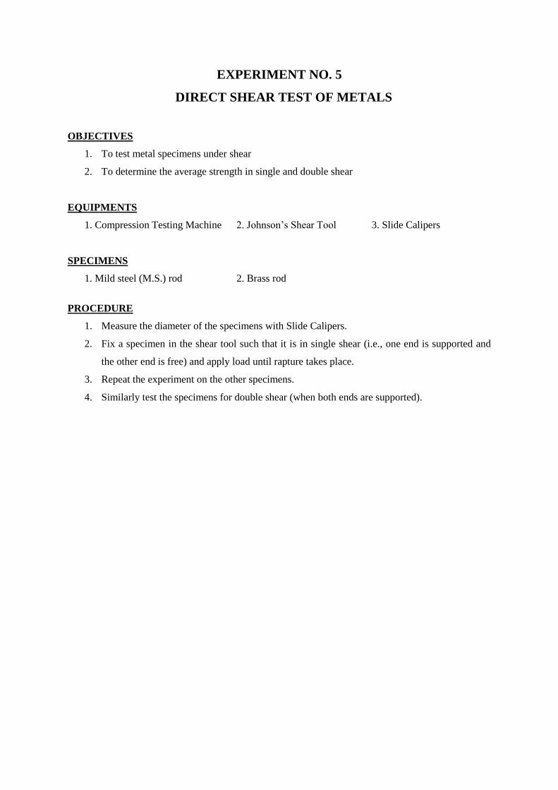
1. Measure the lateral dimensions of the specimen at a full section and at the notch.
2. Set the pointer to read minimum on the graduated disc and note down the initial error as
explained in (3).
A
(0)
b
240
(100) a b 0
Impact Testing Machine
3. Set the hammer block in the position ‘A’ and the pointer along with the carrier, in the position
‘a’ and then release it. When the hammer block stops swinging, the pointer should be in
position ‘b’, if not read the initial error bb = i (this is to be used for high scale).
4. In the same way as described in (3) determine the initial error for the low scale.
Page 35
5. Place and position the sample appropriately in the vise.
6. Raise the pendulum and fix it in proper position. Release the pendulum and record the energy
absorbed.
7. The corrected energy absorbed by the specimen is then found taking into consideration of the
initial error determined earlier. Note the condition of the failed specimen (whether broken or
not).
8. Repeat steps (5) to (7) for each of the specimen supplied.
Page 36
DATA SHEET FOR IMPACT TEST OF METALS
Group Number:
Type of
Specimen
Specimen
Material
Cross-
sectional
Area
Length Volume Scale
used
Initial
Error
(i)
Energy
Absorbed
(E)
Corrected
Energy
(E i)
Modulus of
Toughness
Charpy
Simple
Beam
M.S.
C.I.
Izod
Cantilever
M.S.
C.I.
Charpy
Tension
Rod
M.S.
C.I.
Page 37
CHAPTER 7(A)
HARDNESS TEST OF METALS
7.1 Introduction:
Experiments to determine the ultimate strength of materials or specimens usually involve
subjecting them to tests that eventually destroy the sample. The tests of tensile, compressive, bending
and shear strength using various heavy and expensive equipment or machines are destructive strength
tests, which are most direct ways of knowing the material strength. While they provide the actual
strength of the materials, situations often require the estimation of strengths while preserving the
specimen itself even if it means the estimated strength is empirical or approximate.
For example in cases of expensive materials like diamond, gold etc., finished products like
existing building structures or cases when the exact specimen being tested is also to be used for
structural or other purposes, it is not prudent to destroy the original sample by strength tests. Non-
destructive tests (NDT) become necessary in such cases. They are desirable in several cases because
of their relative simplicity, economy, versatility and preservation of the original samples. In fact the
development of NDT has taken place to such an extent that it is now considered a powerful method of
evaluating existing engineering structures like buildings, bridges, pavements or materials like metals,
concrete, or aggregates.
Since the specimens are not loaded to failure in these tests, their strengths are estimated by
measuring some other properties of the material. Therefore the results are estimations only and do not
provide absolute values of strength. Further development of NDT is encouraged by extensive ongoing
research work in this area.
7.2 Hardness Test of Metals:
Over the last several decades, numerous non-destructive testing methods of metals have been
developed based upon indirect measurements like hardness, rebound number, resonant frequency,
ultrasonic wave propagation, as well as electrical, molecular and acoustic properties. Hardness has
correlation with other mechanical properties of the material; thus hardness tests have wide application
as a non-destructive test of metals.
The term ‘hardness’ refers to the resistance of a metal to permanent deformation to its surface.
This deformation may be in the form of scratching, mechanical wears, indentation or cutting.
Depending on the particular deformation type (or for that matter particular type of stressing) hardness
may be, (i) Indentation hardness test (by indenting), (ii) Scratch hardness test (by scratching), (iii)
Dynamic hardness test (by impact), (iv) Rebound hardness test (by the rebound of a falling ball).
Page 38
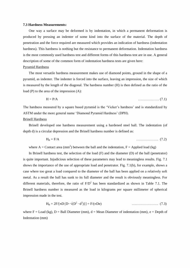
7.3 Hardness Measurements:
One way a surface may be deformed is by indentation, in which a permanent deformation is
produced by pressing an indenter of some kind into the surface of the material. The depth of
penetration and the force required are measured which provides an indication of hardness (indentation
hardness). This hardness is nothing but the resistance to permanent deformation. Indentation hardness
is the most commonly used hardness test and different forms of this hardness test are in use. A general
description of some of the common form of indentation hardness tests are given here:
Pyramid Hardness
The most versatile hardness measurement makes use of diamond points, ground in the shape of a
pyramid, as indenter. The indenter is forced into the surface, leaving an impression, the size of which
is measured by the length of the diagonal. The hardness number (H) is then defined as the ratio of the
load (P) to the area of the impression (A):
H = P/A ……………… (7.1)
The hardness measured by a square based pyramid is the ‘Vicker’s hardness’ and is standardized by
ASTM under the more general name ‘Diamond Pyramid Hardness’ (DPH).
Brinell Hardness
Brinell developed one hardness measurement using a hardened steel ball. The indentation (of
depth d) is a circular depression and the Brinell hardness number is defined as:
HB = F/A ………………. (7.2)
where A = Contact area (mm2) between the ball and the indentation, F = Applied load (kg)
In Brinell hardness test, the selection of the load (F) and the diameter (D) of the ball (penetrator)
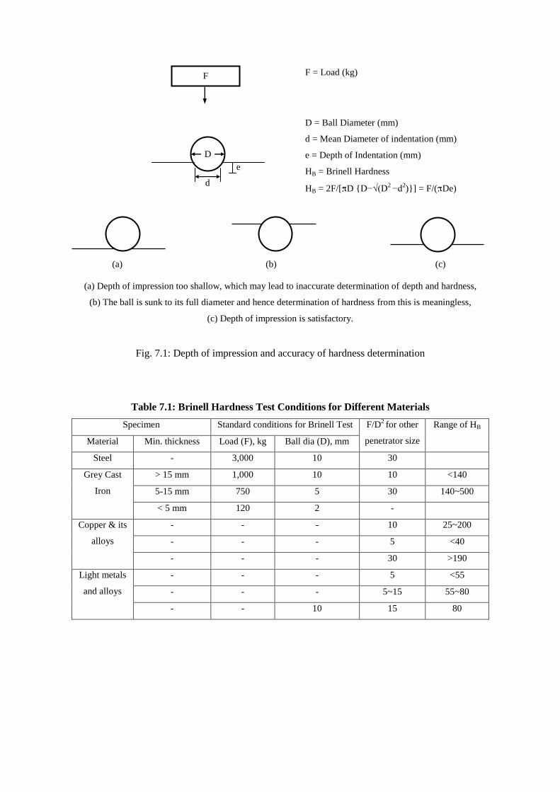
is quite important. Injudicious selection of these parameters may lead to meaningless results. Fig. 7.1
shows the importance of the use of appropriate load and penetrator. Fig. 7.1(b), for example, shows a
case where too great a load compared to the diameter of the ball has been applied on a relatively soft
metal. As a result the ball has sunk to its full diameter and the result is obviously meaningless. For
different materials, therefore, the ratio of F/D2 has been standardized as shown in Table 7.1. The
Brinell hardness number is measured as the load in kilograms per square millimeter of spherical
impression made in the test.
HB = 2F/[ D{D−√(D2 −d
2)}] = F/( De) ….………………. (7.3)
where F = Load (kg), D = Ball Diameter (mm), d = Mean Diameter of indentation (mm), e = Depth of
Indentation (mm)
Page 39
F = Load (kg)
D = Ball Diameter (mm)
d = Mean Diameter of indentation (mm)
e = Depth of Indentation (mm)
HB = Brinell Hardness
HB = 2F/[ D {D−√(D2 −d
2)}] = F/( De)
(a) (b) (c)
(a) Depth of impression too shallow, which may lead to inaccurate determination of depth and hardness,
(b) The ball is sunk to its full diameter and hence determination of hardness from this is meaningless,
(c) Depth of impression is satisfactory.
Fig. 7.1: Depth of impression and accuracy of hardness determination
Table 7.1: Brinell Hardness Test Conditions for Different Materials
Specimen Standard conditions for Brinell Test F/D2 for other
penetrator size
Range of HB
Material Min. thickness Load (F), kg Ball dia (D), mm
Steel - 3,000 10 30
Grey Cast
Iron
> 15 mm 1,000 10 10 <140
5-15 mm 750 5 30 140~500
< 5 mm 120 2 -
Copper & its
alloys
- - - 10 25~200
- - - 5 <40
- - - 30 >190
Light metals
and alloys
- - - 5 <55
- - - 5~15 55~80
- - 10 15 80
F
d
D
e
Page 40
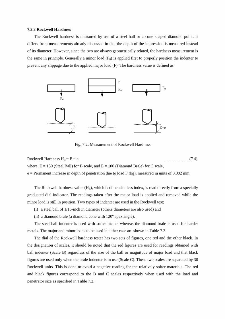
7.3.3 Rockwell Hardness
The Rockwell hardness is measured by use of a steel ball or a cone shaped diamond point. It
differs from measurements already discussed in that the depth of the impression is measured instead
of its diameter. However, since the two are always geometrically related, the hardness measurement is
the same in principle. Generally a minor load (F0) is applied first to properly position the indenter to
prevent any slippage due to the applied major load (F). The hardness value is defined as
Fig. 7.2: Measurement of Rockwell Hardness
Rockwell Hardness HR = E − e ……………….(7.4)
where, E = 130 (Steel Ball) for B scale, and E = 100 (Diamond Brale) for C scale,
e = Permanent increase in depth of penetration due to load F (kg), measured in units of 0.002 mm
The Rockwell hardness value (HR), which is dimensionless index, is read directly from a specially
graduated dial indicator. The readings taken after the major load is applied and removed while the
minor load is still in position. Two types of indenter are used in the Rockwell test;
(i) a steel ball of 1/16-inch in diameter (others diameters are also used) and
(ii) a diamond brale (a diamond cone with 120º apex angle).
The steel ball indenter is used with softer metals whereas the diamond brale is used for harder
metals. The major and minor loads to be used in either case are shown in Table 7.2.
The dial of the Rockwell hardness tester has two sets of figures, one red and the other black. In
the designation of scales, it should be noted that the red figures are used for readings obtained with
ball indenter (Scale B) regardless of the size of the ball or magnitude of major load and that black
figures are used only when the brale indenter is in use (Scale C). These two scales are separated by 30
Rockwell units. This is done to avoid a negative reading for the relatively softer materials. The red
and black figures correspond to the B and C scales respectively when used with the load and
penetrator size as specified in Table 7.2.
F
F0 F0
E E−e
F0
Page 41
Table 7.2: Relevant details for using with a Steel Ball (1/16 ) or Brale Indenter
in a Rockwell Tester
Type of Indenter Scale to be used Minor Load (F0)
kg
Major Load (F)
kg
Steel ball 1/16 dia B 10 90
Diamond Brale C 10 140
Other scales are also used with the Rockwell machine. Each of these scales is indicated by a
symbol (A,D,E,F,G,H,K,L,M,P,R,S and V), which denotes the sizes of the penetrator and the load.
However, Rockwell B and C are the most commonly used scales.
In reporting the Rockwell Hardness values, it is important to mention the scale used. For example,
a hardness measurement reported merely as a number as read form the instrument dial, say 50, has no
meaning whatsoever. In other words the hardness scale is not defined. Thus the hardness numbers
must be prefixed by the letter B or C as appropriate.
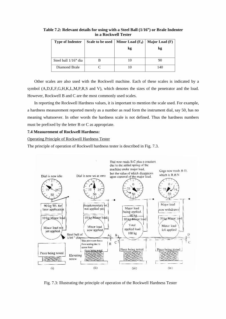
7.4 Measurement of Rockwell Hardness:
Operating Principle of Rockwell Hardness Tester
The principle of operation of Rockwell hardness tester is described in Fig. 7.3.
Fig. 7.3: Illustrating the principle of operation of the Rockwell Hardness Tester
Page 42
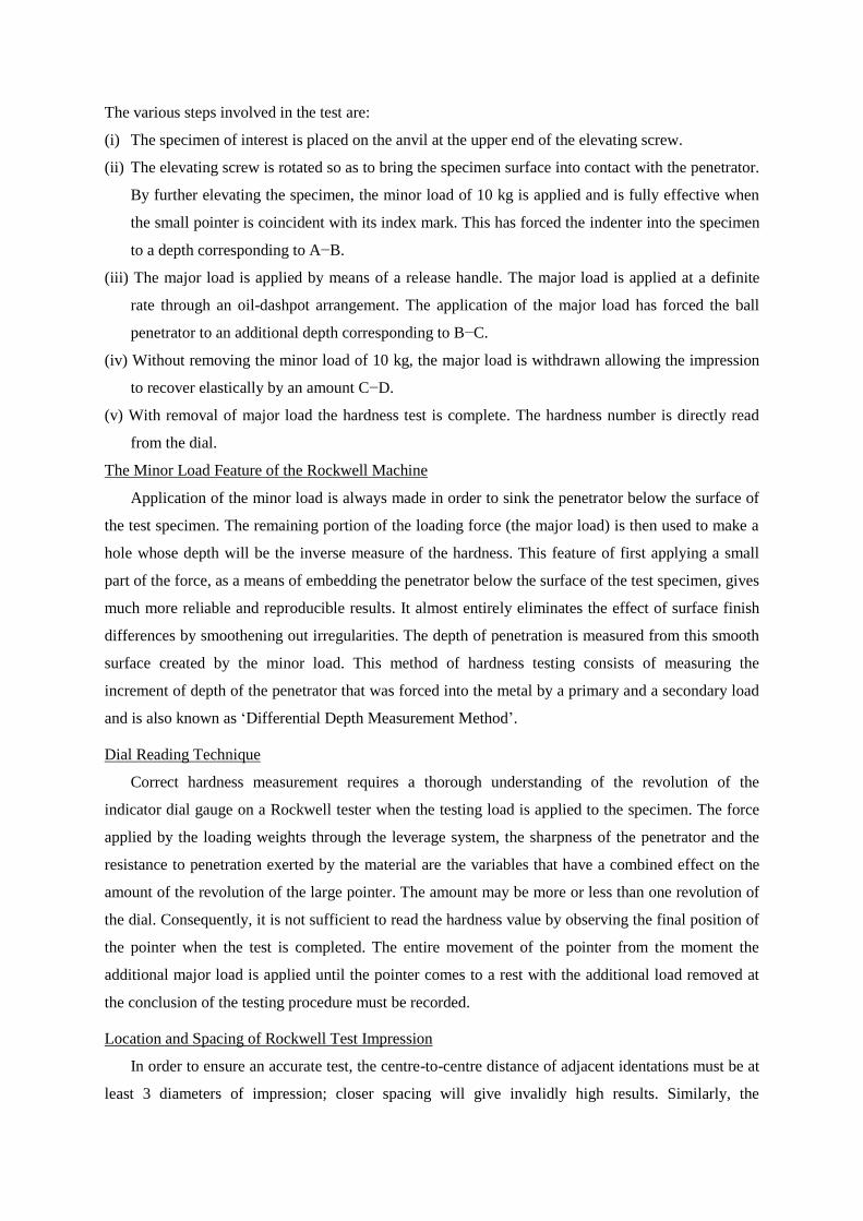
The various steps involved in the test are:
(i) The specimen of interest is placed on the anvil at the upper end of the elevating screw.
(ii) The elevating screw is rotated so as to bring the specimen surface into contact with the penetrator.
By further elevating the specimen, the minor load of 10 kg is applied and is fully effective when
the small pointer is coincident with its index mark. This has forced the indenter into the specimen
to a depth corresponding to A−B.
(iii) The major load is applied by means of a release handle. The major load is applied at a definite
rate through an oil-dashpot arrangement. The application of the major load has forced the ball
penetrator to an additional depth corresponding to B−C.
(iv) Without removing the minor load of 10 kg, the major load is withdrawn allowing the impression
to recover elastically by an amount C−D.
(v) With removal of major load the hardness test is complete. The hardness number is directly read
from the dial.
The Minor Load Feature of the Rockwell Machine
Application of the minor load is always made in order to sink the penetrator below the surface of
the test specimen. The remaining portion of the loading force (the major load) is then used to make a
hole whose depth will be the inverse measure of the hardness. This feature of first applying a small
part of the force, as a means of embedding the penetrator below the surface of the test specimen, gives
much more reliable and reproducible results. It almost entirely eliminates the effect of surface finish
differences by smoothening out irregularities. The depth of penetration is measured from this smooth
surface created by the minor load. This method of hardness testing consists of measuring the
increment of depth of the penetrator that was forced into the metal by a primary and a secondary load
and is also known as ‘Differential Depth Measurement Method’.
Dial Reading Technique
Correct hardness measurement requires a thorough understanding of the revolution of the
indicator dial gauge on a Rockwell tester when the testing load is applied to the specimen. The force
applied by the loading weights through the leverage system, the sharpness of the penetrator and the
resistance to penetration exerted by the material are the variables that have a combined effect on the
amount of the revolution of the large pointer. The amount may be more or less than one revolution of
the dial. Consequently, it is not sufficient to read the hardness value by observing the final position of
the pointer when the test is completed. The entire movement of the pointer from the moment the
additional major load is applied until the pointer comes to a rest with the additional load removed at
the conclusion of the testing procedure must be recorded.
Location and Spacing of Rockwell Test Impression
In order to ensure an accurate test, the centre-to-centre distance of adjacent identations must be at
least 3 diameters of impression; closer spacing will give invalidly high results. Similarly, the
Page 43
minimum permissible distance from the edge of a test specimen to the centre of an impression must be
at least 2.5 times the diameter of the impression.
7.5 Relationship between Hardness Numbers
No precise relationship exists between the several types of hardness numbers. Approximate
relationships have been developed by carrying out tests on the same material using various devices. It
should be borne in mind that these relationships are affected by many factors (materials, heat
treatments etc.) and for this reason too much reliance on them must be avoided.
Brinell (3,000 kg load) and Rockwell hardness numbers may be converted interchangeably with
an accuracy of about 10 percent according to the following relationships:
For RB = 35 ~ 100, BHN = 7300/(130−RB) ……………………….(7.5)
For RC = 20 ~ 40, BHN = 20,000/(100−RC) …………...………….(7.6)
For RC 41, BHN = 25,000/(100−RC) ……………………….(7.7)
where RB and RC denote the Rockwell B and C
Relation between the Hardness Number and other Properties
In general, no precise correlation exists between any indentation hardness and the yield strength
determined in a tension test since the amount of inelastic strain involved in the hardness test is much
greater than in the test for yield strength. However, because of greater similarity in inelastic strain
involved in the test for ultimate tensile strength (UTS) and indentation hardness, empirical relations
have been developed between these two properties. The empirical relationships of Table 7.3 give
approximate tensile strength from Brinell Hardness Number, all of which show that the UTS in ksi is
nearly 40~50% of the BHN.
Table 7.3: Ultimate Tensile Strength from Brinell Hardness Number
Material Tensile Strength (ksi)
For heat treated alloy steels with Brinell No. 250 to 400 0.42 × Brinell No.
For Heat-Treated Carbon Steels as rolled normalized or annealed 0.43 × Brinell No.
For Medium Carbon Steels as rolled normalized or annealed 0.44 × Brinell No.
For Mild Steels normalized or annealed 0.46 × Brinell No.
For non-ferrous rough alloy such as Duralumin Brinell No/2 − 2.0
Page 44
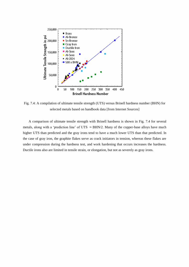
Fig. 7.4: A compilation of ultimate tensile strength (UTS) versus Brinell hardness number (BHN) for
selected metals based on handbook data [from Internet Sources]
A comparison of ultimate tensile strength with Brinell hardness is shown in Fig. 7.4 for several
metals, along with a ‘prediction line’ of UTS BHN/2. Many of the copper-base alloys have much
higher UTS than predicted and the gray irons tend to have a much lower UTS than that predicted. In
the case of gray iron, the graphite flakes serve as crack initiators in tension, whereas these flakes are
under compression during the hardness test, and work hardening that occurs increases the hardness.
Ductile irons also are limited in tensile strain, or elongation, but not as severely as gray irons.
Page 45
EXPERIMENT NO. 7(A)
HARDNESS TEST OF METALS
OBJECTIVES
1. To determine the Rockwell Hardness Number of metal specimens.
2. To find the Brinell Hardness Number from the Rockwell Numbers.
3. To find the ultimate tensile strength of the metal specimens from the Brinell Hardness
Number by using empirical relationships.
4. To compare the empirically obtained tensile strength of the metals with their actual ultimate
tensile strength obtained from tensile test.
EQUIPMENTS
1. Rockwell Hardness Tester 2. Universal Testing Machine and accessories like slide
calipers
SPECIMENS
Plates and tensile strength specimens of
1. Brass 2. Mild Steel (M.S.) 3. High Carbon Steel (H.C.S.) 4. Cast Iron (C.I.)
PROCEDURE
Determination of Rockwell Hardness Number
1. Get the Rockwell Hardness Tester ready for testing.
2. Place the specimen upon the anvil of the tester.
3. Raise the anvil and the test piece by elevating screw until the specimen comes in contact with
the indenter (1/16 -dia Steel ball for Rockwell B and120 Diamond Brale for Rockwell C).
4. Apply the 10 kg minor load on the specimen by moving the pointer of the dial three times.
5. Apply the major load (90 kg for softer materials and 140 kg for harder materials) on the
specimen by pressing the appropriate handle.
6. Return the handle to its original position a few seconds after the application of the major load
(i.e., the major load is withdrawn now).
7. Read the position of the pointer on the scale of the dial as the Rockwell Number (B-scale is
used for softer materials and C-scale for harder materials).
8. Take three readings for each specimen by changing the location of the indentation.
9. Repeat the above steps for each specimen.
Page 46
Determination of Brinell Hardness Number
1. Use the Eqs. (7.5)~(7.7) to calculate the Brinell Hardness Numbers from the Rockwell
Hardness Numbers determined from the above. Note the scale used in each case when the
Rockwell Hardness Number was determined.
Determination of the Ultimate Tensile Strength
1. Use the empirical relationships (Table 7.3) to obtain the tensile strengths from the Brinell
Hardness Numbers.
2. Determine the actual (destructive) tensile strengths of the metal specimens using the
Universal Testing Machine following the procedure outlined in Experiment 3.
Page 47
DATA SHEET FOR HARDNESS TEST OF METALS
Group Number:
Specimen
Material
Applied
Load
(kg)
Scale
Used Indenter R.N.
Mean
R.N. B.N.
Tensile Strength (ksi)
Empirical
Formula
Destructive
Test
Brass
M.S.
H.C.S.
C.I.
Page 48
CHAPTER 7(B)
NON-DESTRUCTIVE TEST OF CONCRETE
7.1 Introduction:
Tests to determine ultimate strength of materials or specimens usually involve subjecting them to
tests that eventually destroy the sample. The tests of tensile, compressive, bending and shear strength
using various heavy and expensive equipment or machines are destructive strength tests, which are
most direct ways of knowing the material strength. While they provide the actual strength of the
materials, situations often require the estimation of strengths while preserving the specimen itself
even if it means the estimated strength is empirical or approximate.
For example in cases of expensive materials like diamond, gold etc., finished products like
existing building structures or cases when the exact specimen being tested is also to be used for
structural or other purposes, it is not prudent to destroy the original sample by strength tests. Non-
destructive tests (NDT) become necessary in such cases. They are desirable in several cases because
of their relative simplicity, economy, versatility and preservation of the original samples. In fact the
development of NDT has taken place to such an extent that it is now considered a powerful method of
evaluating existing engineering structures like buildings, bridges, pavements or materials like metals,
concrete, or aggregates.
Since the specimens are not loaded to failure in these tests, their strengths are estimated by
measuring some other properties of the material. Therefore the results are estimations only and do not
provide absolute values of strength. Further development of NDT is encouraged by extensive ongoing
research work in this area.
7.2 Non-destructive Tests of Concrete:
Over the last sixty years, numerous non-destructive testing methods of concrete have been
developed based upon indirect measurements like hardness, rebound number, resonant frequency,
ultrasonic wave propagation, as well as electrical, nuclear and acoustic properties. Among the testing
methods developed are the hardness tests, elastic rebound tests, penetration/pull out tests, dynamic
vibration tests, radioactive/nuclear methods, magnetic/electrical methods, acoustic emission tests and
others.
7.3 The Schmidt Hammer Test:
The elastic rebound test developed in 1948 by Ernst Schmidt (also known as Schmidt Hammer
Test) is one of the oldest, simplest and most popular non-destructive tests of concrete. This test is also
used in this experiment.
In the Schmidt Hammer Test, a spring loaded mass has a fixed amount of energy imparted to it by
extending the spring to a fixed position; achieved by pressing the plunger against the surface of the
concrete under test. Upon release, the mass rebounds from the plunger, still in contact with the
concrete surface, and the distance traveled by the mass, expressed as a percentage of the initial
Page 49
extension, is called the rebound number. This number is recorded by a rider moving along a graduated
scale.
Fig. 7.1: Schmidt Hammer with (1) plunger, (2) concrete, (3) tubular casing, (4) rider,
(5) scale, (6) mass, (7) release button, (8) spring, (9) spring, (10) catch
The plunger must always be perpendicular to the concrete surface under test, but the rebound
number is affected by position of the hammer relative to the vertical. This is due to the action of
gravity on the travel of the mass in the hammer. Therefore the rebound number of a horizontal surface
below the experimenter (i.e., tested vertically downwards) is smaller than that of a horizontal surface
above, although made of the same concrete. One significant advantage of the Schmidt Hammer Test is
its applicability to surfaces of various inclinations, with scales being calibrated accordingly for
various angles.
The rebound number is largely comparative in nature and as such, is useful in the assessment of
uniformity of concrete within a structure or to check its strength development. It may be used in
deciding when to remove falsework or put the structure into service. Another application of the test is
in assessing abrasion resistance of concrete floors, which depends on its surface hardness.
Despite the advantages of non-destructive tests, particularly the economy, ready applicability and
versatility of the Schmidt Hammer Test, the user should be aware of its limitations and only consider
it as a possible supplement (and not a replacement) of the destructive tests. Some of the significant
aspects and limitations of the test are
1. The rebound number is an arbitrary measure because it depends on the energy stored in the
given spring and the size of the mass.
2. The hammer needs to be used for a smooth surface. Trowelled surfaces should be rubbed
smooth using a carborundum stone.
9. The concrete specimen should be held in an unyielding manner, as jerking during the test
would result in lowering the rebound number.
10. The test is sensitive to local variations in the concrete; e.g., the presence of a large piece of
aggregate immediately underneath the plunger would result in a very high rebound number,
while the presence of a void in a similar position would lead to a low result.
2
1 9 3 6
4 5 10
8
7
Page 50
11. The rebound number is not uniquely related to the strength of concrete, i.e., it depends on its
stiffness as well. Since the stiffness depends on the type of aggregate used, so does the
rebound number.
12. The rebound number measures the properties of only the surface zone of concrete, the depth
within this zone being about 30 mm. Therefore it depends on the surface properties of
concrete like the degree of saturation or carbonation, although they may not affect the
concrete properties at depth.
13. The rebound number should be measured at a number of locations in close proximity, as the
hardness of concrete varies over the surface. However, the testing locations should not be
closer than about 25 mm because of the permanent deformations incurred in tested points.
Page 51
EXPERIMENT NO. 7(B)
NON-DESTRUCTIVE TEST OF CONCRETE
OBJECTIVES
1. To determine the Rebound Number of concrete specimen by the non-destructive Schmidt
Hammer Test.
2. To approximately calculate the compressive strength of the concrete specimen and compare
the result with its compressive strength in a concrete cube/cylinder test.
EQUIPMENTS
1. Schmidt Hammer 2. Compression Testing Machine
SPECIMENS
1. Concrete cube of size 6 6 6 and/or concrete cylinder of 6 diameter and 12 height.
PROCEDURE
1. Unlock the Schmidt Hammer and press the plunger against the specimen.
2. Read the Rebound Number from the scale calibrated on the hammer.
3. Keeping the same alignment of the hammer against the specimen, repeat Step 1 and Step 2 to
obtain several values of the Rebound Number (5~10 in total is often considered adequate).
4. Calculate the mean Rebound Number from the readings taken.
5. Determine the value of from the alignment of the hammer against the specimen.
6. Using the values of mean Rebound Number and in the calibration graphs shown on the
hammer, determine the mean compressive strength and dispersion of strength for the
specimen.
7. Determine the compressive strength of the specimen in a concrete cube/cylinder test.
14. Compare the compressive strengths found in Step 6 and Step 7.
15. Repeat the steps 1 to 8 to evaluate and compare the compressive strengths of all the
specimens.
Page 52
DATA SHEET FOR NON-DESTRUCTIVE TEST OF CONCRETE
Group Number:
Structural
Member
Angle of
Inclination
Spot
No.
Rebound
Number
Mean
Rebound
Number
Non-destructive
Strength
fc'
Dispersion Destructive
Test
fc'
1
2
3
4
5
1
2
3
4
5
1
2
3
4
5
Page 53
CHAPTER 8
TORSION TEST OF STEEL SECTION
8.1 Introduction:
Torsional moment is caused by the action of forces whose resultant does not pass through the
member axis. It may be due to two equal and parallel forces acting at a distance from the member
axis, but any other form of torsion may result in similar effect. For example torsions are caused on
shafts of rotary motors, structural members subjected to eccentric loading (e.g., edge beams),
vertically loaded structural members curved in the horizontal plane (e.g., curved bridges, helical stairs,
grids, balcony girders).
8.2 Shear Center:
As mentioned, torsional moments are caused by forces acting off the axis of a section. Actually
for torsional moments, the axis of the section refers to a point through which a force must be applied
in order for it not to cause any torsional moment in the section. The point is called the shear center of
the section. Therefore, any transverse force applied through the shear center causes no torsion.
Moreover, if a member of any cross-sectional area is twisted, the twist takes place around the shear
center, which remains fixed. For this reason, the shear center is also called the center of twist.
For cross-sectional areas having one axis of symmetry (e.g., T-section, channel section), the shear
center is always located on the axis of symmetry. For those having two axes of symmetry (e.g.,
rectangular, circular, I-section), the shear center coincides with the centroid of the cross-sectional
area.
For thin-walled channel sections, of particular interest in the lab experiment performed, the
location of the shear center can be obtained explicitly by the following expression.
e = b2h
2t/(4I) ………………..….(8.1)
where e = Distance of the shear center from the web, b = Width of the flange, h = Height of the
web, t = Thickness of the section, I = Moment of inertia of the section (shown in Fig. 8.1).
b
t
h
e
Fig. 8.1: Shear Center of Thin-walled Channel section
Page 54
For thin-walled cross-sections, I can be approximated by
I th3/12 + bth
2/2 ………………..….(8.2)
from which e b/(2+h/3b) …………………...(8.3)
8.3 Torsional Stress:
As mentioned in Chapter 5, torsional or twisting moment causes shear stresses and deformations
on the section it acts. The distribution of torsional shear stress varies between different cross-sections.
Fig. 8.2 shows the variation of torsional shear stress for circular, rectangular and arbitrary thin-walled
cross-sections. Whereas the stress varies linearly from the center of a circular section [Fig. 8.2(a)] and
is maximum at the farthest peripheral point from the center, it is the largest at the nearest peripheral
point (and zero at the corners) for rectangular sections [Fig. 8.2(b)] and almost uniformly distributed
over the thickness of closed thin-walled sections, but varies between sections [Fig. 8.2(c)].
(a) (b) (c)
Fig. 8.2: Torsional stress in (a) Circular, (b) Rectangular and (c) Closed thin-walled sections
Of particular interest for the lab experiment are thin-walled open sections. When subjected to
torsional moment, they behave like a rectangular section with the perimeter (p) along centerline
representing the longer side and the thickness (t) of the section representing shorter side of the
rectangle. Therefore its stress distributions are similar to rectangular sections with sides p and t. The
maximum torsional shear stress for such sections occurs at the edges of the longer sides (but not the
corners).
8.4 Torsional Stresses and Deformations for Open Thin-Walled Sections:
As mentioned, open thin walled cross-sections behave like rectangular sections (or area p t)
under the action of torsional moment. The maximum torsional stress and rotations for rectangular
sections (with p and t being the longer and shorter sides) are given by the expressions
(max) = T/( pt 2) …………………...(8.4)
= TL/( pt 3G) …………………...(8.5)
where (max) = Maximum shear stress, = Twisting rotation, T = Twisting moment, L = Length of the
structural member, G = Shear modulus, and = Non-dimensional parameters whose values depend
on the ratio (p/t).
For very thin sections, the ratio (p/t) is quite large and both and tend to assume the value 1/3.
Therefore
Page 55
(max) = 3T/(pt2) ………………..….(8.6)
= 3TL/(pt3G) …………………...(8.7)
For a channel-section of uniform thickness = t, flange width = b and web height = h, the perimeter
along the centerline is p = 2b+h
In the lab experiment, the torsional rotation is calculated for verification with measured rotation
while the maximum shear stress is calculated to check whether the cross-section is within the
proportional limit.
Page 56
EXPERIMENT NO. 8
TORSION TEST OF STEEL SECTION
OBJECTIVES
1. To test a steel specimen under torsion
2. To locate the shear center of the section and compare with analytical result
3. To measure the torsional rotation of the specimen and compare with analytical result
EQUIPMENTS
1. Torsion Testing Machine 2. Steel scale 3. Slide Calipers
SPECIMENS
1. Channel-sectioned Mild steel (M.S.) rod
PROCEDURE
1. Measure cross-sectional dimensions (height, width, thickness) of the channel-sectioned
specimen with Slide Calipers.
2. Calculate the location of the shear center of the channel-section using Eq. (8.3).
3. Use the steel scale to measure the length of the steel specimen as well as the transverse
distances and heights at the hole locations.
4. Put a weight at an extreme hole location (ensuring that the maximum shear stress in the cross-
section calculated by Eq. (8.6) is less than the proportional limit in shear for the material; i.e.,
steel here) and measure again the heights at the hole locations.
5. Calculate the change of heights at the hole locations.
6. Plot the changes of height vs. the transverse distances of the hole locations. From the plot,
locate the shear center of the cross-sectional area and compare it with the theoretical value
calculated in Step 2.
7. From the plot of Step 6, calculate the torsional rotation of the cross-section and compare the
measured rotation with the analytical result obtained from Eq. (8.7).
Page 57
DATA SHEET FOR TORSION TEST OF STEEL SECTION
Group Number:
Width of the section, b = Height of the section, h = Thickness of the section, t =
Distance of the shear center, e =
Perimeter along centerline, p = Shear Modulus, G = Length of Rod, L =
Applied Load, F = Torsional Moment, T =
Torsional Rotation, =
Maximum Torsional Shear Stress, (max) =
Applied
Load
Hole
No.
Transverse
Distance
Height of Hole
Before Loading After Loading Deflection
1
2
3
4
Plot the hole deflection vs. transverse distance and calculate the following from the plot
1. Location of the Shear Center
2. Torsional rotation of the rod
Page 58
CHAPTER 9
COMPRESSION TEST OF HELICAL SPRING
9.1 Introduction:
Helical springs are used in several engineering structures and equipments as load transferring
elements or shock absorbers. Their use as shock absorbers in beds, cushions, pens, watches as well as
in cars, dockyards are well known. In a widening range of applications, they are also being used now
as ground motion transferring and shock absorbing elements (‘base isolators’) underneath several
important building structures or expensive machines to protect the structure itself or the sophisticated
equipment within from impact loads or ground vibrations.
Although the use of helical springs has limited engineering applications mentioned above, the
basic concept of spring (i.e., a structural element undergoing deformation proportional to the load
applied on it) is widely used for numerous structural applications. In fact, most structural elements or
structures under static load follow the spring behavior under static loads.
9.2 Behavior of Closely Coiled Helical Springs:
Helical springs made of rods or wires of circular cross-section (as shown in Fig. 9.1) may be
analyzed in the elastic range by the superposition of shearing stresses. One important assumption need
to be made here is that any one coil of such a spring will be assumed to be in a plane which is nearly
perpendicular to the axis of the spring. This assumption can be made if the adjoining coils are close
enough. As such, a section taken perpendicular to the spring’s rod may be taken to be vertical.
Fig. 9.1: Forces acting on a Closely Coiled Helical Spring
P
P P
V = P
T = PR
R
d = 2r
Page 59
Therefore the forces acting on any section of the spring are
(i) Shearing force, V = P
(ii) Torque, T = PR
where P = axial force applied on the spring, R = distance of the axis of the spring to the centroid
of the rod’s cross-section.
9.3 Combined Shear Stresses in Helical Springs:
The maximum shearing stress at an arbitrary section of the spring is found by superposing the
direct and torsional shear stresses. Direct shearing stress in spring is customarily taken as the average
shearing stress uniformly distributed over the cross-section. Torsional shearing stress having a linear
stress distribution will produce the maximum shear stress at the inner edge of the coil. Therefore, by
superposing one obtains
max = direct + torsion = P/A + Tr/J = P/A (1 + 2R/r) ……….….(9.1)
9.4 Deflection and Stiffness of Helical Springs:
The deflection of a helical spring can be obtained (neglecting the deflection due to direct shear
stress, which is normally small) by using the following relationship
= PR2L/GJ …………..(9.2)
where L = length of the spring’s rod and G = shearing modulus of elasticity (also called the
modulus of rigidity). For a closely coiled spring the length L of the wire may be obtained with
sufficient accuracy as 2 RN, where N is the number of live or active coils of the spring.
= 64 PR3N/Gd
4 ………..…(9.3)
This equation can be used to obtain the deflection of a closely coiled helical spring along its axis
when subjected to either tensile or compressive force P.
The stiffness of a spring, commonly referred to as spring constant, is frequently used to define
the spring’s behavior. The spring constant (commonly denoted by k) is defined as the force required
to produce unit deflection. Thus the spring constant
k = P/ = Gd4/(64R
3N) …………..(9.4)
is a useful quantity. However, the expression of k in Eq. (9.4) is subject to the limitation due to
neglect of the deformation caused by direct shear stresses.
In the laboratory experiment, the axial deflections ( ) of the spring caused by the applied loads
(P) are measured and the best-fit plot of P vs. (a straight line through the origin) drawn in a plain
graph paper. Since, k = P/ from Eq. (9.4), the slope of the plot gives the spring constant, from which
the modulus of rigidity G is obtained as
G = k (64R3N)/d
4 ………..…(9.5)
In order to obtain accurate results, the value of R and more importantly d needs to be measured
very precisely in the lab.
Page 60
EXPERIMENT NO. 9
COMPRESSION TEST OF HELICAL SPRING
OBJECTIVES
1. To test a helical spring under compressive load.
2. To draw the load-deflection curve for the specimen.
3. To determine the stiffness of the spring and shear modulus of the spring material.
4. To calculate the maximum shear stress in the spring coil due to the combination of direct
shear stress and torsional shear stress.
EQUIPMENTS
1. Compression Testing Machine 2. Slide Calipers 3. Scale.
SPECIMEN
1. A helical spring made of high-carbon steel
PROCEDURE
1. Using Slide Calipers, measure the diameter of the spring coil at three locations and determine
the average coil diameter.
2. Measure the inside and outside diameters of the spring and calculate its mean diameter and
mean radius.
3. Record the number of coils in the spring.
4. Set the specimen in the testing machine and observe the scale reading when the loading plate
touches the spring.
5. Apply the load slowly and record the loads and scale readings at constant load interval.
6. Record all the loads and corresponding scale readings while loading the specimen up to a
certain level ensuring that the spring coils do not touch each other and the material of the
spring remains within proportional limit.
Page 61
DATA SHEET FOR COMPRESSION TEST OF HELICAL SPRING
Group Number:
Mean Radius of the Spring = Coil Diameter =
Number of Turns =
Obs.
No.
Readings from Load Average
Deflection Load
Dial
Compressometer
in Loading
Compressometer
in Unloading
1
2
3
4
5
6
7
8
9
10
Calculate the following
1. Maximum direct shear stress in the spring coil
2. Maximum torsional shear stress in the spring coil
3. Maximum combined shear stress in the spring coil
Also draw the load-deflection graph of the helical spring and calculate the following
4. Stiffness of the spring
7. Shear Modulus of the material
Page 62
CHAPTER 10
STATIC BENDING TEST OF TIMBER BEAM
10.1 Theory of Bending:
When beams are subjected to loads, bending stresses are set. The computation of this stress at a
given section of the beam is facilitated by means of bending theory due to M. H. Navier. He
postulated that under a uniform bending moment, initially plane and parallel cross-sections remain
plane during bending and converge to a common center of curvature. This can be visually
demonstrated by drawing a square grid on a flexible beam and then bending the beam (Fig. 10.1).
When subjected to a so-called positive moment (i.e., ‘sagging’ shape), the beam is strained in
compression at the top and in tension at the bottom, and somewhere between there is a line at which
the strain is neither tensile nor compressive. This line of zero strain is called the neutral axis.
Fig. 10.1: Navier’s hypothesis: Originally plane and parallel sections remain plane after bending but
converge onto a common center of curvature
If R is the radius of curvature, then the normal strain of a point located at a distance y (positive
downward) from the neutral axis is given by
= y/R …………(10.1)
If E is the modulus of elasticity of the material, then the corresponding normal stress is
determined by Hooke’s law as
= E = Ey/R …………(10.2)
If M is the bending moment at the section and I is its moment of inertia about the neutral axis,
then the normal stress is also given by
= My/I …………(10.3)
Comparison of Eqs. (10.2) and (10.3) gives
Page 63
= E = My/I
E = My/I …………(10.4)
10.2 Experimental Verification of Navier’s Hypothesis:
Navier’s assumption has been proved correct for all structural materials by strain measurements
on test beams under load (Fig. 10.2); strain gages are fixed along the depth of the beam, and the
variation of strain throughout the section is plotted as the beam is loaded. So long as the beam is
elastic, the neutral axis remains in the same position, and the strains vary proportionately with the
distance from the neutral axis.
Fig. 10.2: Experimental verification of Navier’s hypothesis with strain gages
In general, only the maximum stress (which must be kept within a permissible range) is of
interest. This occurs at the greatest distance y form the neutral axis; in an unsymmetrical section there
are two different values, one for the bottom and another from the top.
10.3 Two Point Loading:
In two-point loading a simply supported beam is loaded at distances ‘a’ from either support,
where L is the span of the beam as shown in Fig. 10.3, the portion of the beam between the loads (P/2
each) is free from any shear and is subjected to purely flexural stress.
The maximum deflection (in the elastic range) at the center of the beam for such a loading is
given by
max = Pa (3L2 4a
2)/48 EI …………(10.5)
If a = L/3, the loading case is known as ‘third point loading’ and the maximum midspan
deflection is
max = 23 PL3/1296 EI …………(10.6)
where P is the total applied load on the beam and EI is the flexural rigidity of the section.
Page 64
P/2 P/2
a (L 2a) a
Fig. 10.3: Shear Force and Bending Moment diagrams for two-point loading
P/2
P/2
Pa/2 Pa/2
P/2 P/2
Under a known value of load P, the deflection at the center span can be measured
experimentally and the above relationships [Eqs. (10.5) or (10.6)] can be used to compute the
value of ‘E’, the modulus of elasticity of the material of the beam. For the purpose of examining
Navier’s hypothesis a two point loading scheme is adopted in the laboratory ensuring a region of
pure bending between the point loads. Strain measurements are made at various distances from
the neutral axis in the central portion of the beam. The value of ‘E’ is determined from the
equation of the best fit straight line for P vs. max.
Page 65
EXPERIMENT NO. 10
STATIC BENDING TEST OF TIMBER BEAM
OBJECTIVES
1. To test a timber beam for static bending under 2-point loading.
2. To draw the corresponding load vs. deflection curve of the beam.
3. To calculate the modulus of elasticity of timber, the flexural rigidity, the maximum tensile
and compressive stresses in the beam.
EQUIPMENTS
1. Beam Testing Machine 2. Deflectometer 3. Steel Scale
4. 2-Point Loading Device 5. Strain Gage
SPECIMEN
1. A 48 long timber beam with a (2 3 ) cross-section.
PROCEDURE
1. Measure the cross-sectional dimensions of the specimen.
2. Place the beam over the platform of the Beam Testing Machine between simple supports and
attach the deflectometer suitably at the bottom of the midspan to read the deflections.
3. Measure the supported span and the loaded span (for 2-point loading) of the specimen and
record the deflectometer constant.
4. Set the machine for the 2-point loading test. Adjust the deflectometer dial to read zero when
the loading starts, i.e., when the loading devices just touch the specimen.
5. Determine the gage length and height of the gage points over the height of the beam. Record
strain gage readings between the gage points at each level.
6. Apply the load slowly and record the loads and deflectometer readings at constant load
intervals up to a certain limit ensuring that the maximum stresses in the beam do not exceed
the proportional limit.
7. Record again the strain gage readings between the gage points and obtain the strains at each
level over the beam height.
8. Draw the load-deflection curve for the beam.
9. Draw the strain diagram over the height of the beam.
Page 66
DATA SHEET FOR STATIC BENDING TEST OF TIMBER BEAM
Group Number:
Effective Span of the Beam = Width of the beam = Depth of the beam =
Obs. No.
Load
Midspan
Deflection
Strain Gage Readings
Point 1 Point 2 Point 3 Point 4 Point 5
1
2
3
4
5
6
7
8
9
10
Draw the (a) load-deflection curve for 2-point loading and
(b) strain diagram over the height of the beam
to calculate the following
1. Modulus of Elasticity
2. Flexural rigidity
3. Maximum compressive stress
4. Maximum tensile stress
Page 67
CHAPTER 11
BIAXIAL BENDING TEST OF METAL SPRINGS
11.1 Introduction:
Biaxial (involving two axes) bending is the bending of a cross-section about two axes of rotation
and often deals with bending about the centroidal axes. If x and y are the centroidal axes of the
cross-sectional area, biaxial bending subjects the section to bending moments Mx and My.
Flexural elements of most three-dimensional structures like beams, columns and footings are
rarely bent about one axis only. Although many simplified structural designs assume structural
elements under uniaxial bending (i.e., bending about one axis only), in most practical applications
they are actually subjected to bending about both the principal axes.
11.2 Biaxial Bending and Combination of Normal Stresses:
Bending however is almost always accompanied by other forces, which result in various types of
normal and shear stresses acting on the cross-section. In addition to uniaxial or biaxial flexural
stresses, most cross-sections are subjected to torsional moment about their geometric axis as well
axial and shear forces. The flexural and axial stresses act normal to the cross-sections, while the shear
forces and torsion give rise to shear stresses (parallel to the plane of the area).
Structures subjected to combined normal (i.e., axial and flexural) stresses provide a very common
case of stress combination, particularly applicable for columns, column footings, pile groups, pre-
stressed concrete beam sections and other structural elements. Such a loading situation can be due to a
concentric axial force accompanied by bending moments about the centroidal axes [as shown in Fig.
11.1(a)] or a biaxially eccentric axial force [Fig. 11.1(b)].
(a) (b)
Fig. 11.1: Cross-sections subjected to (a) Concentric axial load and biaxial bending,
(b) Biaxially eccentric axial load
Since these sections are more often subjected to compressive forces rather than tensile forces, the
formulations and equations in this chapter assume the compressive forces and stresses to be positive
and tensile forces and stresses to be negative.
x
y
x
y P
P
ey
ex Mx
My (x, y) (x, y)
Page 68
For a cross-sectional area subjected to a concentric compressive force P and biaxial moments Mx
and My about the centroidal x and y axes [as shown in Fig. 11.1(a)], the compressive stress at a point
with coordinates (x, y) is given by
(x,y) = P/A + Mx y/Ix + My x/Iy ……………...…(11.1)
where A, Ix and Iy are the area and moments of inertia of the cross-section. For a biaxially
eccentric compressive load P located at a point (ex, ey) in the coordinate axes; i.e., with eccentricities
ey and ex about the x and y axes respectively as shown in Fig. 11.1(b), the biaxial bending moments
are Mx = Pey and My = Pex and the compressive stress at (x, y) is given by
(x,y) = P/A + Pey y/Ix + Pex x/Iy ………………...(11.2)
11.3 Combined Normal Stresses on a Spring Arrangement:
Instead of an integrated solid, structural cross-sections can be made up of discrete parts. For
example, the load carrying area of an arrangement of piles for a pile group or a plate supported by
springs consists of a number of small areas distributed discretely over the entire cross-section, as
shown in Fig. 11.2.
Fig. 11.2: Cross-section consisting of a number of discrete load carrying areas
If the total area consists of N individual discrete spring areas equal to ‘a’ each, the total load
carrying area A = ai = Na. The moment of inertia about the centroidal axis x is Ix = ai yi2 = a yi
2,
while the moment of inertia about the centroidal axis y is Iy = ai xi2
= a xi 2
, where (xi, yi) are the
coordinates of the ith spring. Therefore, Eq. (9.2) (x,y) = P/Na + Pey y/(a yi
2) + Pex x/(a xi
2), and
the normal force on a spring at (x,y) is given by
F(x,y) = (x,y) a = P/N + Pey y/( yi2) + Pex x/( xi
2) ………………….(11.3)
The individual forces on the springs can be determined using Eq. (11.3). In the laboratory
experiment, these forces are compared with forces determined experimentally from the relative
deformation of the springs. Since the spring forces are assumed to be proportional to their
deformations, the force on the ith spring Fi is = P Li/ Li where Li is the shortening of the i
th
spring. In the lab experiment, the uniformity of area and stiffness of all the springs, their consistent
behavior under compression and tension (i.e., so that springs are not separated from the plate under
tension) and the proportionality of force-deflection relationship need to be ensured.
x
y
(xi, yi)
Page 69
EXPERIMENT NO. 11
BIAXIAL BENDING TEST OF METAL SPRINGS
OBJECTIVES
1. To test spring-board arrangements under various types of biaxially eccentric loading.
2. To compare the experimental and the theoretical results.
EQUIPMENTS
1. Rigid Spring-Board arrangements 2. Weights 3. Steel scale 4. Steel Tape
SPECIMENS
1. Short metal springs of similar size
PROCEDURE
1. Choose a wooden board with provisions for inserting spring supports. The board should be
rigid enough to resist excessive deflection and should not collapse under the maximum
anticipated load. However it should be light enough not to excessively load the springs
underneath.
2. Also choose a set of similar springs that are rigid enough not to buckle under the applied
loads but flexible enough to undergo measurable axial deflections.
3. Measure the dimensions of the board as well as the number (N) and possible locations (xi, yi)
of the spring supports.
4. Support the board by a suitable arrangement of springs. Measure the length (L1i) of each
spring support at this stage before applying the loads but supporting the board only.
5. Apply load (P, Case I) by placing it slowly at any suitable position on the board.
6. Measure the coordinates (ex, ey) of the location of the weight with respect to the centroid of
the board. Also measure the length (L2i) of each spring support.
7. Calculate the deflection of each spring support ( Li) by subtracting their initial lengths and
calculate the load (Fi(expt)) carried by each support.
8. Calculate theoretically the load carried by each spring (Fi(theory)) and compare with the
experimental results.
9. Repeat the process for any other set of springs/loading arrangements (Case II and others).
Page 70
DATA SHEET FOR BIAXIAL BENDING TEST OF METAL SPRINGS
Group Number:
Applied Load, P = Eccentricity, ex = Eccentricity, ey =
Number of Springs, N = x i2 = y i
2 =
Spring
No.
xi yi Fi (theory)
= P [1/N + xi ex/ xi2 + yi ey/ yi
2]
L1i L2i Li Fi (expt)
= P Li/ Li
1
2
3
4
5
6
7
8
9
Page 71
CHAPTER 12
BUCKLING TEST OF SLENDER COLUMNS
12.1 Introduction:
It has been discussed in Chapters 3 and 4 that the ultimate (axial) load carried by a structural
member is given by
Pu = uA ………………………....(3.1)
where u is the appropriate ultimate strength (tensile or compressive as the case may be) of the
material, and A is the cross-sectional area of the member. While the above equation for determining
the ultimate capacity of an axially loaded member is always true in the case of tension member, for
the compression member (i.e. column), however, this is true only in the certain range of slenderness
of the member concerned. For example, in the case of stocky column (short column) the above
equation will hold good and the ultimate load will be obtained through complete classification of the
cross-section of the member. On the other hand for relatively slender column (long column), the
column will fail at a load lower than that given by equation 12.1. The cross-section of the column may
be entirely or at least partly elastic, when this type of failure takes place. This is known as the bucking
effect, often an important consideration in the design of compression members. Therefore,
compression members may have two different modes of failure. One is by exhaustion of the capacity
(strength) of the section (Eq. 12.1) and the other is due to lack of stiffness (instability effect).
12.2 Euler’s Theory for Slender Columns:
Consider an initially straight elastic structural member under compressive end-loads being in
equilibrium at a deformed position (Fig. 12.1).
Fig. 12.1: Axially loaded structural member in deformed equilibrium position
If E, I, L are the material’s modulus of elasticity, sectional moment of inertia and length of the
member, the generalized equation for the deflected shape of the member is
v(x) = C1 cos x + C2 sin x [where 2= P/EI] ..………….(12.1)
Considering the boundary conditions, v(0) = 0 C1 = 0, and v(L) = 0 C2 sin ( L) = 0
Either C2 = 0 v(x) = C1 cos x + C2 sin x = 0, which is a trivial solution …..…..…….(12.2)
Or L = n = n /L P = 2 EI = n
2 2EI/L
2 ..……..…….(12.3)
v P
x
L
P A B
v v
x
v P
A
P
M
Page 72
Eq. (10.3) provides a set of solutions for the load P in order to cause deflection of the column. The
smallest of force is obtained by putting n = 1, resulting in the critical load of the column as
Pcr = 2EI/L
2 ……...………….(12.4)
The critical load shown in Eq. (12.4) is also called the buckling load or Euler load of the column,
named after Leonhard Euler who was the first to derive it in 1757. It is an important part of the theory
of structures and is one of the oldest structural formulae still in use. In Eq. (12.4), it is noted that I is
the minimum moment of inertia (Imin) of the column section.
Euler’s solution presents the buckling of column as a bifurcation problem; i.e., according to it the
column would not deflect at all until it reaches the first critical load (= 2EI/L
2), where its deflection is
arbitrary. After exceeding this load, the column returns to its un-deflected position until it reaches the
second critical load (= 42EI/L
2), and so on.
Fig. 12.2: Euler’s bifurcation solution for structural member under compressive load
12.3 Modifications of Euler’s Buckling Theory:
The conclusion drawn from Euler’s formulation that the column would deflect only at certain
critical loads and remain un-deflected otherwise is very much in conflict with the behavior of real
columns, which would deflect from the onset of loading. Moreover Euler’s theory cannot predict the
failure of compression members, which is expected in buckling.
The discrepancy and limitations can be attributed to the assumptions in deriving the formula; i.e.,
that the column is perfectly straight, the applied load is concentric, the support condition is pin-
pinned, the material follows Hooke’s law and that there is no residual stress in the column (which is
inappropriate for steel).
Effect of Initial Imperfection
The assumption that the columns are initially straight can be overcome by a formulation that
considers an initially deformed (imperfect) column, which should however satisfy the column’s
boundary conditions. The solution of the resulting differential equation for a simply supported column
provides the results shown in Fig. 10.3(a), where v0i and v(L/2) are the initial and final midspan
v0
P
P=2EI/L
2
P=42EI/L
2
Page 73
deflection of the column before and after loading, while the axial loads P and Pcr are as explained
before.
Instead of the earlier conclusion (based on Euler’s formulation) that the column remains in the
initial un-deflected shape except at critical loads (Fig. 10.2), it shows that the deflection starts from
the onset of loading. It is a more realistic conclusion, supporting observations from tests on real
slender columns.
Effect of Load Eccentricity (End Moments)
Real columns are seldom, if ever, subjected to concentric loads. Therefore the axial loads are
almost always accompanied by end moments. The effect of load eccentricity or end moments on the
structural response of a simply supported slender column is shown in Fig. 12.3(b). This provides
results similar to the effect of initial imperfection, in that it also shows that the deflection starts from
the onset of loading. In this curve, e is the eccentricity of the axial load.
However, both the results from initial imperfection and end moments also show that the column
will eventually reach the critical buckling load Pcr at infinite deflection. The limitations of this
conclusion is demonstrated if material nonlinearity if taken into account.
Fig. 1: Effect of (1) Column Imperfection and (2) Load Eccentricity
0
0.2
0.4
0.6
0.8
1
0 5 10 15 20
(1) v(L/2)/v0i, or (2) v(L/2)/e
P/P
cr
Graph (1) Graph (2)(a) (b)
(a) (b)
Fig. 12.3: Effect of (a) Column Imperfection, (b) Load Eccentricity
Page 74
Effect of Material Nonlinearity
As mentioned, Fig. 12.3 can successfully model the deflection of a slender column from the onset
of loading but cannot predict its eventual failure, which is a natural conclusion of the buckling
behavior. Clearly, the notion of reaching the critical buckling load Pcr at infinite deflection is not
realistic because the material nonlinearity and failure criteria would cause a failure of the column at a
smaller load and a much smaller deflection.
Fig. 10.4 shows the results for a simply supported slender column of elasto-plastic material,
which is subjected to axial load and end moments. The results show that for decreasing values of the
plastic moment Mp, the maximum load reached by a column gets smaller. In fact, it is slightly above
60% of the critical load for Mp = 200 k-ft and above 30% of the critical load for Mp = 50 k-ft. Since
beyond these points, the loads carried by the column in equilibrium decreases with deflection, they
can be identified as the failure loads of the columns.
Although these are results from a particular study, they demonstrate the potential effect of
material nonlinearity if the column is deformed large enough. They also show that in general, real
columns would fail at loads much smaller than the critical load predicted by Euler.
Effect of Residual Stresses
Residual stresses are particularly significant for steel structures in that they cause internal stresses
even before the loading begins. These initial stresses may lead to earlier yielding of the structure. For
slender columns, this implies more pronounced effect of nonlinearity and, as shown before, a more
significant loss of column strength.
Effect of End Conditions
The discussion so far has concentrated on the derivation of the critical load for a simply supported
(pin-ended) column. But in real situation columns may have a wide range of support condition giving
Effect of Material Nonlinearity
0.0
0.2
0.4
0.6
0.8
1.0
0 1 2 3 4 5
v(L/2)/e
P/P
cr
Mp=200 k-ft Mp=100 k-ft Mp= 50 k-ft
Fig. 12.4: (a) Elasto-plastic M- relationship, (b) Effect of Material Nonlinearity
EI
M
Mp
Page 75
rise to the concept of end-restrained column. The presence of end restraint affect the column strength
and it is desirable to make proper allowance for this in both the analysis and the design of column.
Use of the Euler type of approach to study the elastic buckling of end-restrained columns enables the
elastic critical load to be related directly to the stiffness of the restraint at either end, through the
concept of effective length. This requires that the critical load formula (Eq. 12.4) be modified as:
Pcr = 2EImin/(kL)
2 =
2EImin/Le
2 ……...………….(12.5)
where k is the effective length factor and kL (= Le) is the effective length, which is defined as the
length of the equivalent pin-ended column that would have the same elastic critical load as the actual
end-restrained column. The effective length factor (k) for several standard cases of rigid end restraint
is shown in Table 12.1. For more generalized support conditions, structural designers often refer to an
alignment chart for determining k for braced and unbraced frames based on the relative stiffness of the
beams and columns at both ends.
In laboratory tests on slender columns the experimental buckling loads are often found to be
lower than the corresponding theoretical values due to the reasons mentioned before. However, they
may sometimes exceed the theoretically calculated critical loads if the fixity of end supports is not
properly accounted for.
Table 12.1 Effective Length Factors for Various End Conditions
End Conditions of the Column Length Factor, k
Hinged-Hinged 1.0
Hinged-Fixed 0.7
Fixed-Fixed 0.5
Fixed-Free (i.e., cantilever) 2.0
12.4 Critical Stress and Column Design Curve:
From the critical buckling loads derived in the earlier discussion, one can derive expressions for
corresponding stresses, which may be a more convenient expression from the design point of view.
Dividing the Eq. (12.5) through by area A
cr = Pcr/A = 2E(Imin/A)/(kL)
2 =
2E/(Le/rmin)
2
cr = 2E/( )
2 ……...………….(12.6)
where cr is the critical stress, rmin [= (Imin/A)] is the minimum radius of gyration of the column
section and (= Le/rmin) is defined as the slenderness ratio. Eq. 12.6 is plotted as the graph of cr
against and this is known as the Euler column curve of a given material.
If the material is elasto-plastic with a yield stress ( y) it is obvious that if the elastic cr is greater
than y, plastic squashing rather than elastic buckling takes place. This gives the sharp cutout to
column strength curve at the lower slenderness ratios. In practice the cut-off is not sharp as indicated
but curves gradually, due to inelastic buckling. The result is a column design curve with the initial
portion (below a critical slenderness ratio c) corresponding to material yielding and the latter portion
Page 76
to elastic column buckling. For structural members under compression, the AISC-ASD (AISC
American Society of Steel Construction, ASD Allowable Stress Design) column design curve is
shown in Fig. 10.5. The design curve accounts for the uncertainties in loading and design conditions
with factors of safety.
AISC-ASD Column Design Curve
0.0
0.1
0.2
0.3
0.4
0.5
0.6
0 1 2 3 4 5
= / c
all/ y
Fig. 12.5: AISC-ASD Column Design Curve
Page 77
EXPERIMENT NO. 12
BUCKLING TEST OF SLENDER COLUMNS
OBJECTIVES
1. To determine the buckling loads of slender columns of different lengths and end conditions.
2. To compare the experimental and the theoretical critical loads.
3. To draw the column strength curve.
EQUIPMENTS
1. Column Testing Apparatus 2. Weights 3. Slide Calipers 4. Steel scale
SPECIMENS
1. High tensile steel column of different lengths.
PROCEDURE
1. Measure the length and the mean diameter of the column to be tested
2. Place the column in the column testing apparatus with the both end hinged..
3. Apply load by placing equal weights on both pans. Give a small lateral force to deflect the
column laterally. Increase the load if the column straightens back upon removal of the lateral
force.
4. Continue the process until the applied load is just sufficient to hold the column in a bend
condition; i.e., when the column does not straighten back after removal of lateral load. Record
this load as the critical load.
5. Perform the experiment for columns with different lengths.
6. Repeat the above steps (1) to (5) for the following two end conditions:
(a) One end hinged and one end fixed (b) Both end fixed.
7. Calculate the theoretical buckling load for each loading case.
8. Draw the column strength curve including the theoretical buckling curves.
Page 78
DATA SHEET FOR BUCKLING TEST OF SLENDER COLUMNS
Group Number:
Modulus of Elasticity (E) of Column Material =
Support
Conditions
Colm
Diameter
(d)
Area
(A)
Minm
Radius
of Gyr.
(rmin)
Colm
Length
(L)
Effective
Length
(Le)
Slenderness
Ratio
(= Le/rmin)
Critical
Force
(Pcr)
cr (exp)
(= Pcr/A)
cr (theory)
(= 2E/
2)
Both Ends
Hinged
Fixed
and Hinged
Both Ends
Fixed
Draw the critical stress vs. slenderness ratio diagram for both experimental and theoretical results.