Structural Properties of Utility FunctionsWalrasian Demand

Econ 2100 Fall 2017

Lecture 4, September 7

Outline

1 Structural Properties of Utility Functions

1 Local Non Satiation2 Convexity3 Quasi-linearity

2 Walrasian Demand

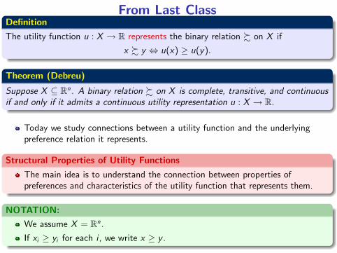
From Last ClassDefinitionThe utility function u : X → R represents the binary relation % on X if

x % y ⇔ u(x) ≥ u(y).

Theorem (Debreu)

Suppose X ⊆ Rn . A binary relation % on X is complete, transitive, and continuousif and only if it admits a continuous utility representation u : X → R.

Today we study connections between a utility function and the underlyingpreference relation it represents.

Structural Properties of Utility FunctionsThe main idea is to understand the connection between properties ofpreferences and characteristics of the utility function that represents them.

NOTATION:We assume X = Rn .If xi ≥ yi for each i , we write x ≥ y .

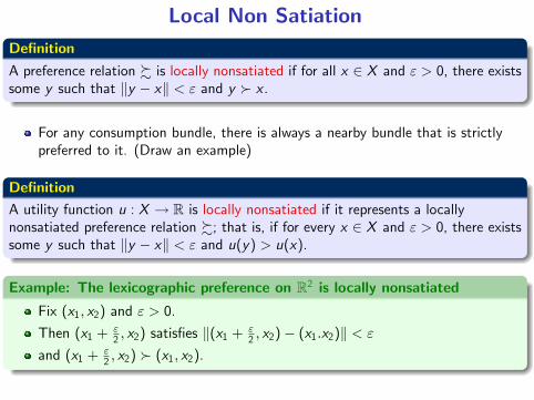
Local Non SatiationDefinitionA preference relation % is locally nonsatiated if for all x ∈ X and ε > 0, there existssome y such that ‖y − x‖ < ε and y � x .

For any consumption bundle, there is always a nearby bundle that is strictlypreferred to it. (Draw an example)

DefinitionA utility function u : X → R is locally nonsatiated if it represents a locallynonsatiated preference relation %; that is, if for every x ∈ X and ε > 0, there existssome y such that ‖y − x‖ < ε and u(y) > u(x).

Example: The lexicographic preference on R2 is locally nonsatiatedFix (x1, x2) and ε > 0.

Then (x1 + ε2 , x2) satisfies ‖(x1 +

ε2 , x2)− (x1.x2)‖ < ε

and (x1 + ε2 , x2) � (x1, x2).

Local Non Satiation and Strict Monotonicity

Proposition

If % is strictly monotone, then it is locally nonsatiated.

Proof.

Let x be given, and let y = x + εn e, where e = (1, ..., 1).

Then we have yi > xi for each i .

Strict monotonicity implies that y � x .Note that

||y − x || =

√√√√ n∑i=1

( εn

)2=

ε√n< ε.

Thus % is locally nonsatiated.

Shapes of Functions

DefinitionsSuppose C is a convex subset of X . A function f : C → R is:

concave iff (αx + (1− α)y) ≥ αf (x) + (1− α)f (y)

for all α ∈ [0, 1] and x , y ∈ C ;strictly concave if

f (αx + (1− α)y) > αf (x) + (1− α)f (y)for all α ∈ (0, 1) and x , y ∈ X such that x 6= y ;quasiconcave if

f (x) ≥ f (y)⇒ f (αx + (1− α)y) ≥ f (y)for all α ∈ [0, 1];strictly quasiconcave if

f (x) ≥ f (y) and x 6= y ⇒ f (αx + (1− α)y) > f (y)for all α ∈ (0, 1).

Convex Preferences

DefinitionsA preference relation % is

convex ifx % y ⇒ αx + (1− α)y % y for all α ∈ (0, 1)

strictly convex if

x % y and x 6= y ⇒ αx + (1− α)y � y for all α ∈ (0, 1)

Convexity says that taking convex combinations cannot make the decisionmaker worse off.

Strict convexity says that taking convex combinations makes the decisionmaker better off.

QuestionWhat does convexity imply for the utility function representing %?

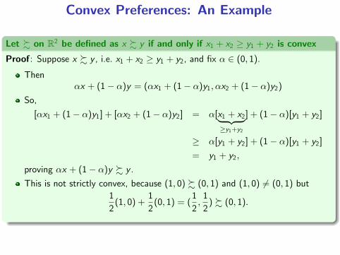
Convex Preferences: An Example

Let % on R2 be defined as x % y if and only if x1 + x2 ≥ y1 + y2 is convexProof: Suppose x % y , i.e. x1 + x2 ≥ y1 + y2, and fix α ∈ (0, 1).

Thenαx + (1− α)y = (αx1 + (1− α)y1, αx2 + (1− α)y2)

So,

[αx1 + (1− α)y1] + [αx2 + (1− α)y2] = α[x1 + x2︸ ︷︷ ︸≥y1+y2

] + (1− α)[y1 + y2]

≥ α[y1 + y2] + (1− α)[y1 + y2]= y1 + y2,

proving αx + (1− α)y % y .This is not strictly convex, because (1, 0) % (0, 1) and (1, 0) 6= (0, 1) but

12(1, 0) +

12(0, 1) = (

12,12) % (0, 1).

Convexity and Quasiconcave Utility Functions

Convexity is equivalent to quasi concavity of the corresponding utility function.

Proposition

If u represents %, then:1 % is convex if and only if u is quasiconcave;2 % is strictly convex if and only if u is strictly quasiconcave.

Convexity of % implies that any utility representation is quasiconcave, but notnecessarily concave.

Proof.Question 5b. Problem Set 2, due next Tuesday.

Quasiconcave Utility and Convex Upper ContoursProposition

Let % be a preference relation on X represened by u : X → R. Then, the uppercontour set is a convex subset of X if and only if u is quasiconcave.

Proof.Suppose that u is quasiconcave.

Fix z ∈ X , and take any x , y ∈% (z).Wlog, assume u(x) ≥ u(y ), so that u(x) ≥ u(y ) ≥ u(z), and let α ∈ [0, 1].

By quasiconcavity of u,u(z) ≤ u(y ) ≤ u(αx + (1 − α)y ),

so αx + (1 − α)y % z .Hence αx + (1 − α)y belongs to % (z), proving it is convex.

Now suppose the better-than set is convex.

Let x , y ∈ X and α ∈ [0, 1], and suppose u(x) ≥ u(y ).Then x % y and y % y , and so x and y are both in % (y ).Since % (y ) is convex (by assumption), then αx + (1 − α)y % y .Since u represents %,

u(αx + (1 − α)y ) ≥ u(y )Thus u is quasiconcave.

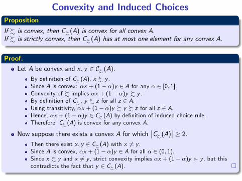
Convexity and Induced ChoicesProposition

If % is convex, then C%(A) is convex for all convex A.If % is strictly convex, then C%(A) has at most one element for any convex A.

Proof.

Let A be convex and x , y ∈ C%(A).By definition of C%(A), x % y .Since A is convex: αx + (1 − α)y ∈ A for any α ∈ [0, 1].Convexity of % implies αx + (1 − α)y % y .By definition of C%, y % z for all z ∈ A.Using transitivity, αx + (1 − α)y % y % z for all z ∈ A.Hence, αx + (1 − α)y ∈ C%(A) by definition of induced choice rule.Therefore, C%(A) is convex for any convex A.

Now suppose there exists a convex A for which∣∣C%(A)∣∣ ≥ 2.

Then there exist x , y ∈ C%(A) with x 6= y .Since A is convex, αx + (1 − α)y ∈ A for all α ∈ (0, 1).Since x % y and x 6= y , strict convexity implies αx + (1 − α)y � y , but thiscontradicts the fact that y ∈ C%(A).

Quasi-linear UtilityDefinition

The function u : Rn → R is quasi-linear if there exists a function v : Rn−1 → Rsuch that u(x ,m) = v(x) +m.

We usually think of the n-th good as money (the numeraire).

Proposition

The preference relation % on Rn admits a quasi-linear representation if and only1 (x ,m) % (x ,m′) if and only if m ≥ m′, for all x ∈ Rn−1 and all m,m′ ∈ R;2 (x ,m) % (x ′,m′) if and only if (x ,m +m′′) % (x ′,m′ +m′′), for all x ∈ Rn−1and m,m′,m′′ ∈ R;

3 for all x , x ′ ∈ Rn−1, there exist m,m′ ∈ R such that (x ,m) ∼ (x ′,m′).

1 Given two bundles with identical goods, the consumer always prefers the onewith more money.

2 Adding (or subtracting) the same monetary amount does not change rankings.3 Monetary transfers can always be used to achieve indifference.

Proof.Question 5c. Problem Set 2, due next Tuesday.

Quasi-linear Preferences and Utility

Proposition

Suppose that the preference relation % on Rn admits two quasi-linearrepresentations: v(x) +m, and v ′(x) +m, where v , v ′ : Rn−1 → R. Then thereexists c ∈ R such that v ′(x) = v(x)− c for all x ∈ Rn−1.

Proof.Exercise

Homothetic Preferences and Utility

Homothetic preferences are also useful in many applications, in particular foraggregation problems and macroeconomics.

DefinitionThe preference relation % on X is homothetic if for all x , y ∈ X ,

x ∼ y ⇒ αx ∼ αy for each α > 0

Proposition

The continuous preference relation % on Rn is homothetic if and only if it isrepresented by a utility function that is homogeneous of degree 1.

A function is homogeneous of degree r if f (αx) = αr f (x) for any x and α > 0.

Proof.Question 5d. Problem Set 2, due next Tuesday.

Demand Theory

Main Questions

Suppose the consumer uses her income to purchase goods (commodities) atthe exogenously given prices:

What are the optimal consumption choices?How do they depend on prices and income?

Typically, we answer this questions solving a constrained optimization problemusing calculus.

That means the utility function must be not only continuous, but alsodifferentiable.

Differentiability is not a property we can derive from preferences.

That is, however, not necessary and we can talk about optimal choices evenwhen preferences are not necessarily represented by a utility function.

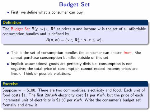
Budget SetFirst, we define what a consumer can buy.

Definition

The Budget Set B(p,w) ⊂ Rn at prices p and income w is the set of all affordableconsumption bundles and is defined by

B(p,w) = {x ∈ Rn+ : p · x ≤ w}.

This is the set of consumption bundles the consumer can choose from. Shecannot purchase consumption bundles outside of this set.

Implicit assumptions: goods are perfectly divisible; consumption is nonnegative; the total price of consumption cannot exceed income; prices arelinear. Think of possible violations.

Exercise

Suppose w = $100. There are two commodities, electricity and food. Each unit offood costs $1. The first 20Kwh electricity cost $1 per Kwh, but the price of eachincremetal unit of electricity is $1.50 per Kwh. Write the consumer’s budget setformally and draw it.

Walrasian Demand

Main IdeaThe optimal consumption bundles are those that are preferred to all otheraffordable bundles.

DefinitionGiven a preference relation %, the Walrasian demand correspondencex∗ : Rn++ × R+ → Rn+ is defined by

x∗(p,w) = {x ∈ B(p,w) : x % y for any y ∈ B(p,w)}.

By definition, for any x∗ ∈ x∗(p,w)x∗ % x for any x ∈ B(p,w).

Walrasian demand equals the induced choice rule given the preference relation% and the available set B(p,w):

x∗(p,w) = C%(B(p,w)).

More implicit assumptions: income is non negative; prices are strictly positive.

Walrasian Demand With Utility

Although we do not need the utility function to exist to define Walrasiandemand, if a utility function exists there is an equivalent definition.

DefinitionGiven a utility function u : Rn+ → R, the Walrasian demand correspondencex∗ : Rn++ × R+ → Rn+ is defined byx∗(p,w) = arg max

x∈B(p,w )u(x) where B(p,w) = {x ∈ Rn+ : p · x ≤ w}.

As before,x∗(p,w) = C%(B(p,w)).

and for any x∗ ∈ x∗(p,w)u(x∗) ≥ u(x) for any x ∈ B(p,w).

We can derive some properties of Walrasian demand directly from assumptionson preferences and/or utility.

Walrasian Demand Is Homogeneous of Degree Zero

PropositionWalrasian demand is homogeneous of degree zero: for any α > 0

x∗(αp, αw) = x∗(p,w)

Proof.For any α > 0,

B(αp, αw) = {x ∈ Rn+ : αp · x ≤ αw} = {x ∈ Rn+ : p · x ≤ w} = B(p,w)because α is a scalar

Since the constraints are the same, the optimal choices must also be thesame.

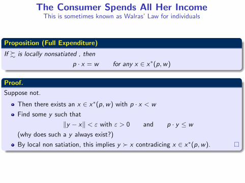
The Consumer Spends All Her IncomeThis is sometimes known as Walras’Law for individuals

Proposition (Full Expenditure)

If % is locally nonsatiated , thenp · x = w for any x ∈ x∗(p,w)

Proof.Suppose not.

Then there exists an x ∈ x∗(p,w) with p · x < wFind some y such that

‖y − x‖ < ε with ε > 0 and p · y ≤ w(why does such a y always exist?)

By local non satiation, this implies y � x contradicing x ∈ x∗(p,w).

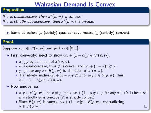
Walrasian Demand Is ConvexProposition

If u is quasiconcave, then x∗(p,w) is convex.If u is strictly quasiconcave, then x∗(p,w) is unique.

Same as before (u (stricly) quasiconcave means % (strictly) convex).

Proof.

Suppose x , y ∈ x∗(p,w) and pick α ∈ [0, 1].First convexity: need to show αx + (1− α)y ∈ x∗(p,w).

x % y by definition of x∗(p,w ).u is quasiconcave, thus % is convex and αx + (1 − α)y % y .y % z for any z ∈ B(p,w ) by definition of x∗(p,w ).Transitivity implies αx + (1 − α)y % z for any z ∈ B(p,w ); thusαx + (1 − α)y ∈ x∗(p,w ).

Now uniqueness.

x , y ∈ x∗(p,w ) and x 6= y imply αx + (1 − α)y � y for any α ∈ (0, 1) becauseu is strictly quasiconcave (% is strictly convex).Since B(p,w ) is convex, αx + (1 − α)y ∈ B(p,w ), contradictingy ∈ x∗(p,w ).

Walrasian Demand Is Non-Empty and Compact

Proposition

If u is continuous, then x∗(p,w) is nonempty and compact.

We already proved this as well.

Proof.Define A by

A = B(p,w) = {x ∈ Rn+ : p · x ≤ w}

This is a closed and bounded (i.e. compact, set) and

x∗(p,w) = C%(A) = C%(B(p,w))

where % are the preferences represented by u.Then x∗(p,w) is the set of maximizers of a continuous function over acompact set.

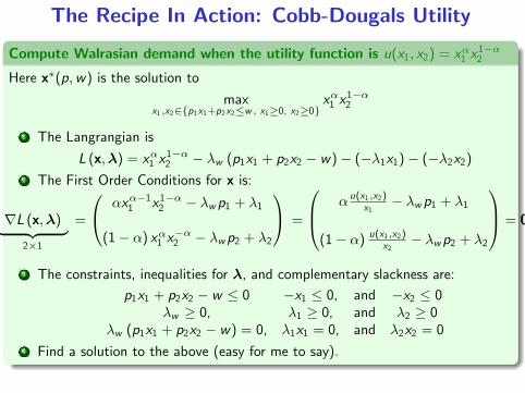
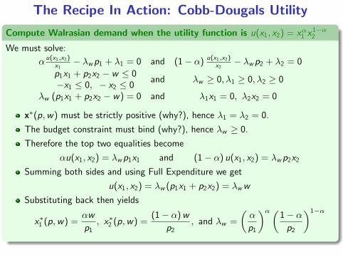
Walrasian Demand: ExamplesHow do we find the Walrasian Demand?

Need to solve a constrained maximization problem, usually using calculus.

Question 6, Problem Set 2; due next Tuesday.For each of the following utility functions, find the Walrasian demandcorrespondence. (Hint: pictures may help)

1 u(x) =n∏i=1xαii with αi > 0 (Cobb-Douglas).

2 u(x) = min{α1x1, α2x2, ..., αnxn} with αi > 0 (generalized Leontief).3 u(x) =

∑ni=1 αixi for αi > 0 (generalized linear).

4 u(x) =[∑n

i=1 αixρi

] 1ρ (generalized CES).

Can we do the second one using calculus?

How about the third? Do we need calculus?

Constant elasticity of substitution (CES) preferences are the most commonlyused homothetic preferences. Many preferences are a special case of CES.

An Optimization Recipe

How to solve max f (x) subject to gi (x) ≤ 0 with i = 1, ..,m

1 Write the Langrange function L : Rn × Rm → R as

L (x,λ) = f (x)−m∑i=1

λigi (x)

2 Write the First Order Conditions:n×1︷ ︸︸ ︷

∇L (x,λ) = ∇f (x)−m∑i=1

λi∇gi (x) = 0︸ ︷︷ ︸∂f (x)∂xj−

m∑i=1λi∂gi (x)∂xj

=0 for all j=1,..,n

3 Write constraints, inequalities for λ, and complementary slackness conditions:gi (x) ≤ 0 with i = 1, ..,m

λi ≥ 0 with i = 1, ..,mλigi (x) = 0 with i = 1, ..,m

4 Find the x and λ that satisfy all these and you are done...hopefully.

The Recipe In Action: Cobb-Dougals Utility

Compute Walrasian demand when the utility function is u(x1, x2) = xα1 x1−α2

Here x∗(p,w) is the solution tomax

x1,x2∈{p1x1+p2x2≤w , x1≥0, x2≥0}xα1 x

1−α2

1 The Langrangian is

L (x,λ) = xα1 x1−α2 − λw (p1x1 + p2x2 − w)− (−λ1x1)− (−λ2x2)

2 The First Order Conditions for x is:

∇L (x,λ)︸ ︷︷ ︸2×1

=

αxα−11 x1−α2 − λw p1 + λ1

(1− α) xα1 x−α2 − λw p2 + λ2

=

α u(x1,x2)x1− λw p1 + λ1

(1− α) u(x1,x2)x2− λw p2 + λ2

= 0

3 The constraints, inequalities for λ, and complementary slackness are:p1x1 + p2x2 − w ≤ 0 −x1 ≤ 0, and −x2 ≤ 0

λw ≥ 0, λ1 ≥ 0, and λ2 ≥ 0λw (p1x1 + p2x2 − w) = 0, λ1x1 = 0, and λ2x2 = 0

4 Find a solution to the above (easy for me to say).

The Recipe In Action: Cobb-Dougals Utility

Compute Walrasian demand when the utility function is u(x1, x2) = xα1 x1−α2

We must solve:α u(x1,x2)x1

− λw p1 + λ1 = 0 and (1− α) u(x1,x2)x2− λw p2 + λ2 = 0

p1x1 + p2x2 − w ≤ 0−x1 ≤ 0, − x2 ≤ 0

and λw ≥ 0, λ1 ≥ 0, λ2 ≥ 0

λw (p1x1 + p2x2 − w) = 0 and λ1x1 = 0, λ2x2 = 0

x∗(p,w) must be strictly positive (why?), hence λ1 = λ2 = 0.

The budget constraint must bind (why?), hence λw ≥ 0.Therefore the top two equalities become

αu(x1, x2) = λw p1x1 and (1− α) u(x1, x2) = λw p2x2Summing both sides and using Full Expenditure we get

u(x1, x2) = λw (p1x1 + p2x2) = λww

Substituting back then yields

x∗1 (p,w) =αwp1

, x∗2 (p,w) =(1− α)w

p2, and λw =

(α

p1

)α(1− αp2

)1−α

Next Week

More Properties of Walrasian Demand.

Indirect Utility.

Comparative Statics.

Expenditure Minimization.