Structural Sparse Tracking

Tianzhu Zhang1,2 Si Liu3 Changsheng Xu2,4 Shuicheng Yan5 Bernard Ghanem1,6

Narendra Ahuja1,7 Ming-Hsuan Yang8

1 Advanced Digital Sciences Center 2 Institute of Automation, CAS 3 Institute of Information Engineering, CAS4 China-Singapore Institute of Digital Media 5 National University of Singapore 6 King Abdullah University of Science and Technology

7 University of Illinois at Urbana-Champaign 8 University of California at Merced

Abstract

Sparse representation has been applied to visual tracking

by finding the best target candidate with minimal reconstruc-

tion error by use of target templates. However, most sparse

representation based trackers only consider holistic or lo-

cal representations and do not make full use of the intrinsic

structure among and inside target candidates, thereby mak-

ing the representation less effective when similar objects ap-

pear or under occlusion. In this paper, we propose a novel

Structural Sparse Tracking (SST) algorithm, which not on-

ly exploits the intrinsic relationship among target candidates

and their local patches to learn their sparse representations

jointly, but also preserves the spatial layout structure among

the local patches inside each target candidate. We show that

our SST algorithm accommodates most existing sparse track-

ers with the respective merits. Both qualitative and quantita-

tive evaluations on challenging benchmark image sequences

demonstrate that the proposed SST algorithm performs fa-

vorably against several state-of-the-art methods.

1. Introduction

Visual tracking aims to estimate the states of a moving

target in a video. It has long been one of the most im-

portant and fundamental topics in computer vision with a

plethora of applications such as surveillance, vehicle naviga-

tion, human computer interface, and human motion analysis,

to name a few. Despite numerous object tracking method-

s [33, 26, 35, 30, 17, 24] having been proposed in recent

years, it remains a challenging task to develop a robust al-

gorithm for complex and dynamic scenes due to the factors

such as partial occlusions, illumination, pose, scale, camera

motion, background clutter, and viewpoint.

Most tracking algorithms are developed from the discrim-

inative or generative perspectives. Discriminative approach-

es formulate the tracking problem as a binary classification

task in order to find the decision boundary for separating

the target object from the background [2, 6, 9, 10, 3, 16].

Avidan [2] combines a set of weak classifiers into a strong

one and develops an ensemble tracking method. Collins et

al. [6] demonstrate that the most discriminative features can

be learned online to separate the target object from the back-

ground. In [9], Grabner et al. propose an online boosting

method to update discriminative features and a semi-online

boosting algorithm [10] to handle the drifting problem in ob-

ject tracking. Babenko et al. [3] introduce multiple instance

learning into online object tracking where samples are con-

sidered within positive and negative bags or sets. Kalal et

al. [16] propose the P-N learning algorithm to exploit the un-

derlying structure of positive and negative samples to learn

classifiers for object tracking.

In contrast, generative tracking methods typically learn

a model to represent the target object and then use it to

search for the image region with minimal reconstruction er-

ror [5, 7, 14, 1, 25, 31, 18]. Black et al. [5] learn an off-line

subspace model to represent the object of interest for track-

ing. The mean shift tracking algorithm [7] models a target

with nonparametric distributions of features (e.g., color pix-

els) and locates the object with mode shifts. The Frag tracker

[1] addresses the partial occlusion problem by modeling ob-

ject appearance with histograms of local patches. The IVT

method [25] utilizes an incremental subspace model to adapt

appearance changes. Kwon et al. [18] use multiple obser-

vation models to cover a wide range of appearance changes,

caused by pose and illumination variation, for tracking. Most

of these methods use holistic representations to describe ob-

jects and hence do not handle occlusions or distracters well.

Recently, sparse representation based generative tracking

methods have been developed for object tracking [21, 20, 19,

23, 22, 34, 37, 36, 4, 15, 13, 39, 42, 41, 29]. These track-

ers can be categorized based on the representation schemes

into global, local, and joint sparse appearance models as

shown in Figure 1. In [21, 19, 23, 22, 34, 4], the sparse

trackers represent each target candidate xi as a sparse linear

combination of target templates T that can be dynamically

updated to account for appearance changes. These models

have been shown to be robust against partial occlusions with

demonstrated performance for tracking. However, all these

methods model a target object as a single entity as shown in

150978-1-4673-6964-0/15/$31.00 ©2015 IEEE

(a) global sparse appearance model (b) local sparse appearance model

(c) joint sparse appearance model (d) structural sparse appearance model

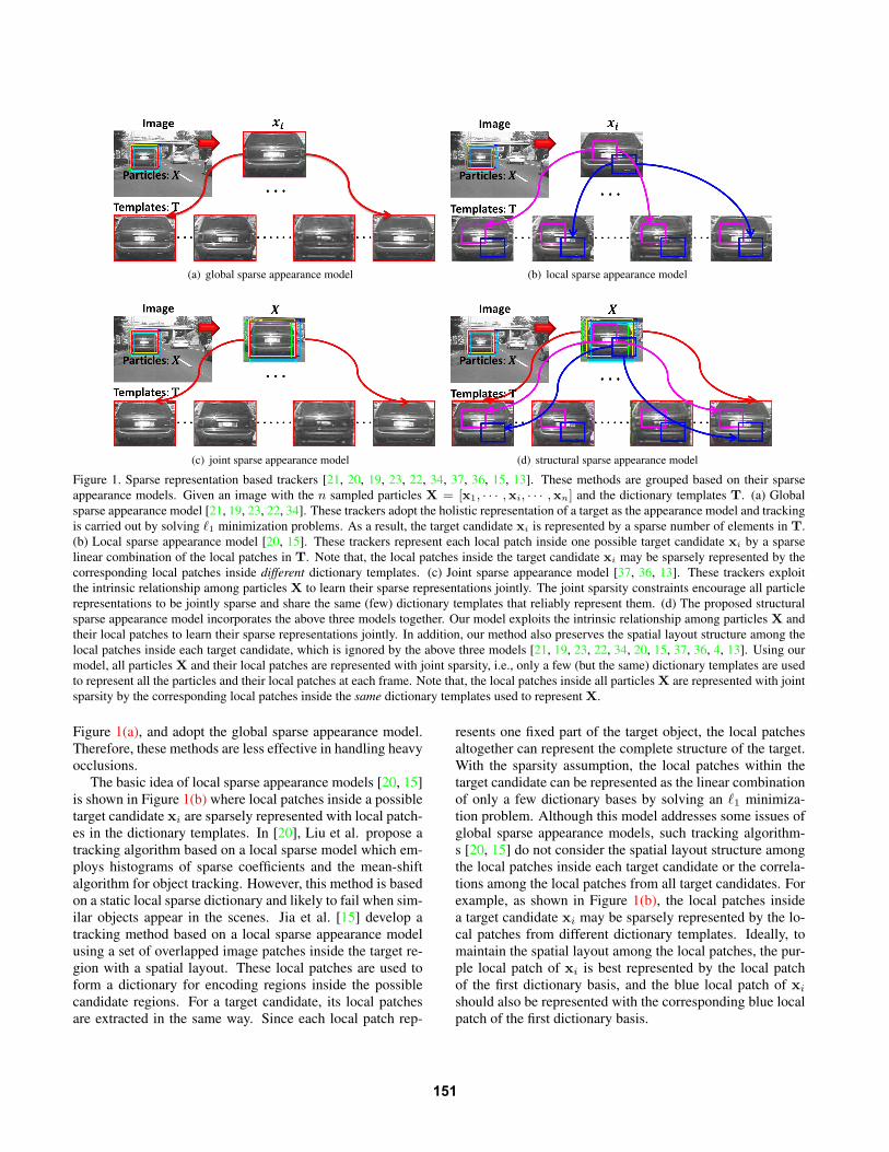
Figure 1. Sparse representation based trackers [21, 20, 19, 23, 22, 34, 37, 36, 15, 13]. These methods are grouped based on their sparse

appearance models. Given an image with the n sampled particles X = [x1, · · · ,xi, · · · ,xn] and the dictionary templates T. (a) Global

sparse appearance model [21, 19, 23, 22, 34]. These trackers adopt the holistic representation of a target as the appearance model and tracking

is carried out by solving ℓ1 minimization problems. As a result, the target candidate xi is represented by a sparse number of elements in T.

(b) Local sparse appearance model [20, 15]. These trackers represent each local patch inside one possible target candidate xi by a sparse

linear combination of the local patches in T. Note that, the local patches inside the target candidate xi may be sparsely represented by the

corresponding local patches inside different dictionary templates. (c) Joint sparse appearance model [37, 36, 13]. These trackers exploit

the intrinsic relationship among particles X to learn their sparse representations jointly. The joint sparsity constraints encourage all particle

representations to be jointly sparse and share the same (few) dictionary templates that reliably represent them. (d) The proposed structural

sparse appearance model incorporates the above three models together. Our model exploits the intrinsic relationship among particles X and

their local patches to learn their sparse representations jointly. In addition, our method also preserves the spatial layout structure among the

local patches inside each target candidate, which is ignored by the above three models [21, 19, 23, 22, 34, 20, 15, 37, 36, 4, 13]. Using our

model, all particles X and their local patches are represented with joint sparsity, i.e., only a few (but the same) dictionary templates are used

to represent all the particles and their local patches at each frame. Note that, the local patches inside all particles X are represented with joint

sparsity by the corresponding local patches inside the same dictionary templates used to represent X.

Figure 1(a), and adopt the global sparse appearance model.

Therefore, these methods are less effective in handling heavy

occlusions.

The basic idea of local sparse appearance models [20, 15]

is shown in Figure 1(b) where local patches inside a possible

target candidate xi are sparsely represented with local patch-

es in the dictionary templates. In [20], Liu et al. propose a

tracking algorithm based on a local sparse model which em-

ploys histograms of sparse coefficients and the mean-shift

algorithm for object tracking. However, this method is based

on a static local sparse dictionary and likely to fail when sim-

ilar objects appear in the scenes. Jia et al. [15] develop a

tracking method based on a local sparse appearance model

using a set of overlapped image patches inside the target re-

gion with a spatial layout. These local patches are used to

form a dictionary for encoding regions inside the possible

candidate regions. For a target candidate, its local patches

are extracted in the same way. Since each local patch rep-

resents one fixed part of the target object, the local patches

altogether can represent the complete structure of the target.

With the sparsity assumption, the local patches within the

target candidate can be represented as the linear combination

of only a few dictionary bases by solving an ℓ1 minimiza-

tion problem. Although this model addresses some issues of

global sparse appearance models, such tracking algorithm-

s [20, 15] do not consider the spatial layout structure among

the local patches inside each target candidate or the correla-

tions among the local patches from all target candidates. For

example, as shown in Figure 1(b), the local patches inside

a target candidate xi may be sparsely represented by the lo-

cal patches from different dictionary templates. Ideally, to

maintain the spatial layout among the local patches, the pur-

ple local patch of xi is best represented by the local patch

of the first dictionary basis, and the blue local patch of xi

should also be represented with the corresponding blue local

patch of the first dictionary basis.

151

The joint sparse appearance model [37, 36, 13] is shown

in Figure 1(c), which is motivated by the following obser-

vations. In particle filter-based tracking methods, particles

at and around the target are randomly sampled according

to a zero-mean Gaussian distribution based on the previous

states. Each particle shares dependencies with other parti-

cles and their corresponding images are likely to be similar.

In [37], learning the representation of each particle is viewed

as an individual task and a multi-task learning with joint s-

parsity for all particles is employed. In [36], the low-rank

sparse learning is applied to learn the sparse representations

of all particles jointly. In [13], the multi-task multi-view join-

t sparse representation is adopted for tracking. The methods

based on joint sparse appearance models [37, 36, 13, 38, 40]

aim to improve the tracking performance by exploiting the

intrinsic relationship among particles. Moreover, due to the

joint optimization among all particles X, this model is com-

putationally efficient. However, such models still use the

holistic representations to describe object appearance.

Motivated by the above three models, we propose a novel

structural sparse appearance model as shown in Figure 1(d),

which has the following differences. First, the proposed

structural sparse appearance model incorporates the above

three models together and is shown to be less sensitive

to partial occlusion [20, 15], and computationally efficien-

t [37, 36, 13] by considering the correlations among the tar-

get candidates. Second, the proposed model exploits the in-

trinsic relationship among not only the particles X, but also

the corresponding local image patches to learn their sparse

representations jointly. Third, the proposed model preserves

the spatial layout structure among the local patches insid-

e each target candidate, which is ignored in the previous s-

parse trackers [21, 19, 23, 22, 34, 20, 15, 37, 36, 4, 13]. As

shown in Figure 1(d), since all particles X and their local

patches are represented with joint sparsity, only a few (but

the same) dictionary templates are used to represent all the

particles and their local patches at each frame. Note that, the

local patches inside all particles X are represented with joint

sparsity by the corresponding local patches inside the same

dictionary templates used to represent X.

Based on the structural sparse appearance model, we pro-

pose a computationally efficient structural sparse tracking

(SST) algorithm within the particle filter framework. Here,

all particles and their local patches are represented via the

proposed structural sparse appearance model, and the next

target state is the particle that it and its local patches have the

highest similarity with target dictionary templates and their

corresponding patches. Unlike previous methods, our pro-

posed SST algorithm not only exploits the intrinsic relation-

ship among particles and their local patches to learn their

sparse representations jointly, but also preserves the spatial

layout structure among the local patches inside each target

candidate. This helps locate the target more accurately and

is less sensitive to partial occlusion. In our SST formulation,

we use the ℓp,q mixed-norm regularizer, which is optimized

Figure 2. The spatial layout for local patches sampling. Note that,

any other local patch sampling methods can also be adopted.

using an Accelerated Proximal Gradient (APG) method for

fast convergence. In addition, we show that existing ℓ1 track-

er [22], LST [15], and MTT [37] methods are the special

cases of our SST formulation.

2. Structural Sparse Tracking

In this section, we give a detailed description of our parti-

cle filter based tracking method that use the structural sparse

appearance model to represent particles and their local patch-

es jointly. Particles are sampled at and around the previous

object location to predict the state st of the target at time

t, from which we crop the region of interest yt in the cur-

rent image and normalize it to the template size. The state

transition function p(st|st−1) is modeled by an affine mo-

tion model with a diagonal Gaussian distribution. The obser-

vation model p(yt|st) reflects the similarity between an ob-

served image region yt corresponding to a particle st and the

templates of the current dictionary. In this work, p(yt|st) is

computed by a function of the reconstruction error obtained

by linearly representing yt and its local patches using the

template dictionary. The particle that maximizes this func-

tion is selected to be the tracked target at each time instance.

Next, we show how to use the structural sparse appearance

model to represent particles and their local patches in details.

2.1. Structural Sparse Appearance Model

Given the image set of the target templates T =[T1,T2, · · · ,Tm], we sample K local image patches insid-

e each target region with a spatial layout. For simplicity,

the spatial layout as shown in Figure 2 is used. Note that,

any other local patch sampling methods can also be adopt-

ed. After sampling local patches, they are used to form a

dictionary for encoding local patches inside any candidate

region. For the k-th local image patch among these m target

templates, we obtain the corresponding dictionary templates

Dk =[dk1 ,d

k2 , · · · ,d

km

]∈ R

dk×m, where k = 1, · · · ,K;

K is the number of local patches sampled within the target

region; dk is the dimension of the k-th image patch vector;

and m is the number of target templates. Each column in

Dk is obtained by ℓ2 normalization on the vectorized gray-

scale image observations extracted from T. Each local patch

represents one fixed part of the target, and hence the local

patches altogether can represent the complete structure of the

target. Since the image patches are collected from many tem-

plates, this dictionary captures the commonality of different

templates and is able to represent various forms of these part-

152

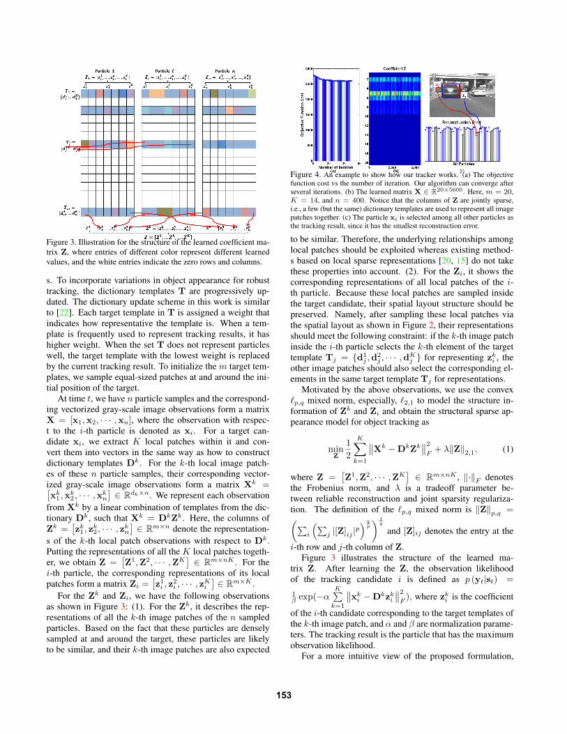
Figure 3. Illustration for the structure of the learned coefficient ma-

trix Z, where entries of different color represent different learned

values, and the white entries indicate the zero rows and columns.

s. To incorporate variations in object appearance for robust

tracking, the dictionary templates T are progressively up-

dated. The dictionary update scheme in this work is similar

to [22]. Each target template in T is assigned a weight that

indicates how representative the template is. When a tem-

plate is frequently used to represent tracking results, it has

higher weight. When the set T does not represent particles

well, the target template with the lowest weight is replaced

by the current tracking result. To initialize the m target tem-

plates, we sample equal-sized patches at and around the ini-

tial position of the target.

At time t, we have n particle samples and the correspond-

ing vectorized gray-scale image observations form a matrix

X = [x1,x2, · · · ,xn], where the observation with respec-

t to the i-th particle is denoted as xi. For a target can-

didate xi, we extract K local patches within it and con-

vert them into vectors in the same way as how to construct

dictionary templates Dk. For the k-th local image patch-

es of these n particle samples, their corresponding vector-

ized gray-scale image observations form a matrix Xk =[xk1 ,x

k2 , · · · ,x

kn

]∈ R

dk×n. We represent each observation

from Xk by a linear combination of templates from the dic-

tionary Dk, such that Xk = DkZk. Here, the columns of

Zk =[zk1 , z

k2 , · · · , z

kn

]∈ R

m×n denote the representation-

s of the k-th local patch observations with respect to Dk.

Putting the representations of all the K local patches togeth-

er, we obtain Z =[Z1,Z2, · · · ,ZK

]∈ R

m×nK . For the

i-th particle, the corresponding representations of its local

patches form a matrix Zi =[z1i , z

2i , · · · , z

Ki

]∈ R

m×K .

For the Zk and Zi, we have the following observations

as shown in Figure 3: (1). For the Zk, it describes the rep-

resentations of all the k-th image patches of the n sampled

particles. Based on the fact that these particles are densely

sampled at and around the target, these particles are likely

to be similar, and their k-th image patches are also expected

Figure 4. An example to show how our tracker works. (a) The objective

function cost vs the number of iteration. Our algorithm can converge after

several iterations. (b) The learned matrix X ∈ R20×5600. Here, m = 20,

K = 14, and n = 400. Notice that the columns of Z are jointly sparse,

i.e., a few (but the same) dictionary templates are used to represent all image

patches together. (c) The particle xi is selected among all other particles as

the tracking result, since it has the smallest reconstruction error.

to be similar. Therefore, the underlying relationships among

local patches should be exploited whereas existing method-

s based on local sparse representations [20, 15] do not take

these properties into account. (2). For the Zi, it shows the

corresponding representations of all local patches of the i-

th particle. Because these local patches are sampled inside

the target candidate, their spatial layout structure should be

preserved. Namely, after sampling these local patches via

the spatial layout as shown in Figure 2, their representations

should meet the following constraint: if the k-th image patch

inside the i-th particle selects the k-th element of the target

template Tj = {d1j ,d

2j , · · · ,d

Kj } for representing zki , the

other image patches should also select the corresponding el-

ements in the same target template Tj for representations.

Motivated by the above observations, we use the convex

ℓp,q mixed norm, especially, ℓ2,1 to model the structure in-

formation of Zk and Zi and obtain the structural sparse ap-

pearance model for object tracking as

minZ

1

2

K∑

k=1

∥∥Xk −DkZk∥∥2F+ λ‖Z‖2,1, (1)

where Z =[Z1,Z2, · · · ,ZK

]∈ R

m×nK , ‖·‖F denotes

the Frobenius norm, and λ is a tradeoff parameter be-

tween reliable reconstruction and joint sparsity regulariza-

tion. The definition of the ℓp,q mixed norm is ‖Z‖p,q =(∑

i

(∑j |[Z]ij |

p) q

p

) 1

q

and [Z]ij denotes the entry at the

i-th row and j-th column of Z.

Figure 3 illustrates the structure of the learned ma-

trix Z. After learning the Z, the observation likelihood

of the tracking candidate i is defined as p (yt|st) =

1βexp(−α

K∑k=1

∥∥xki −Dkzki

∥∥2F), where zki is the coefficient

of the i-th candidate corresponding to the target templates of

the k-th image patch, and α and β are normalization parame-

ters. The tracking result is the particle that has the maximum

observation likelihood.

For a more intuitive view of the proposed formulation,

153

we visualize an empirical example of the learned sparse rep-

resentation in Figure 4 and show an example of how the

proposed SST tracker works. Given all particles X (sam-

pled around the tracked car), their local patches (Xk, k =1, · · · ,K) can be sampled based on the spatial layout as

shown in Figure 2. Then, based on the corresponding dic-

tionary templates (Dk, k = 1, · · · ,K), we can learn the rep-

resentation matrix Z =[Z1,Z2, · · · ,ZK

]by solving (1).

Note that a brighter color squares in Z represents a larg-

er value in the corresponding entry. Clearly, columns of Z

are jointly sparse, i.e., a few (but the same) dictionary tem-

plates are used to represent all the image patches together.

The particle xi is determined as the current tracking result

yt because the reconstruction error of its image patches with

respect to the target templates is the smallest among all par-

ticles. Since particle xj corresponds to a misaligned image

of the target, it has a bigger reconstruction error and cannot

be represented well by T.

2.2. Discussion

As discussed in the introduction and in Figure 1, exist-

ing sparse tracking methods [21, 20, 19, 23, 22, 34, 37, 36,

15, 13] can be categorized as global, local, and joint sparse

appearance models based on the representation schemes.

Motivated by the above three models, we propose a nov-

el structural sparse appearance model as shown in (1) for

object tracking. Our formulation (1) is generic and incor-

porates the above three models together to have their prop-

erties. It is worth emphasizing the difference between the

proposed SST algorithm and several related tracking meth-

ods [21, 20, 19, 23, 22, 34, 37, 36, 15, 13].

• Global sparse appearance models for tracking [21, 19,

23, 22, 34]. In (1), when K = 1 (only 1×1 as shown in

Figure 2), with ℓ1,1 mixed norm is adopted, the formu-

lation (1) reduces to a global sparse appearance model,

which modes a target by one single entity, and learns

the sparse representations of target candidates indepen-

dently without considering their intrinsic relationships.

• Local sparse appearance models for tracking [20, 15].

In (1), with the image patch sampling methods as [20,

15] and the ℓ1,1 mixed norm, our formulation (1) re-

duces to a local sparse representation model, which

does not consider the correlations of image patches a-

mong multiple target candidates or the spatial layout

structure of image patches inside each target candidate.

• Joint sparse appearance model for tracking [37, 36, 13].

In (1), when K = 1 (only 1 × 1 as shown in Figure 2),

with ℓ2,1 mixed norm, the formulation (1) reduces to a

joint sparse representation model, which considers the

intrinsic relationships among target candidates. Howev-

er, this model uses a holistic object representation.

• The structural sparse appearance model for tracking.

Our tracker SST has the following properties: (1). It

considers both the global and local sparsity constraints.

(2). It considers the intrinsic relationships among not

only the target candidates, but also their local image

patches. (3). It considers the spatial layout structure

of image patches inside each target candidate.

Based on the above discussion, it is clear that our formu-

lation in (1) is generic and most tracking methods based on

sparse representation are its special cases. Our formulation

(1) does not only maintain the sparse properties of the exist-

ing three models, but also exploit the spatial layout structure

of image patches inside each target candidate.

3. Experimental Results

To evaluate the performance of our tracker, we conduct

extensively experiments on 20 publicly available challenging

image sequences. These sequences contain complex scenes

with challenging factors for visual tracking, e.g., cluttered

background, moving camera, fast movement, large variation

in pose and scale, partial occlusion, shape deformation and

distortion (See Figure 5). For comparison, we run 14 state-

of-the-art algorithms with the same initial position of the tar-

get. These algorithms are the online multiple instance learn-

ing (MIL) [3], online Adabost boosting (OAB) [9], track-

ing by detection (TLD) [16], Struck [11], circulant structure

tracking (CST) [12], part-based visual tracking (PT) [32], re-

al time compressive tracking (RTCT) [34], ℓ1 tracking (ℓ1T)

[22], local sparse tracking (LST) [15], multi-task tracking

(MTT) [37], incremental visual tracking (IVT) [25], distri-

bution field tracking (DFT) [27], fragments-based (Frag) [1],

and local-global tracking (LGT) [28] methods. Here, MIL,

OAB, TLD, Struck, CST, and PT are discriminative track-

ers, and others (IVT, DFT, Frag, LGT, RTCT, ℓ1T, MTT,

and LST) are generative trackers. In addition, RTCT and

ℓ1T, LST, and MTT are based on global, local, and joint s-

parse models, respectively. By comparing with these differ-

ent kinds of methods, we demonstrate the effectiveness of

our proposed SST. For fair comparisons, we use the pub-

licly available source or binary codes provided by the au-

thors. The default parameters are set for initialization.

For all reported experiments, we set η = 0.1, λ = 0.5,

the number of image patches K = 14 as shown in Fig-

ure 2, the number of templates m = 20, the number of

particles n = 400 (the same for ℓ1T and MTT). The vari-

ances of affine parameters for particle sampling is set to

(0.01, 0.0005, 0.0005, 0.01, 4, 4). The template size d is set

to half the size of the target object manually initialized in the

first frame. The proposed algorithm is implemented in MAT-

LAB and runs at 0.45 seconds per frame on a 2.80 GHz Intel

Core2 Duo machine with 8GB memory. We will make the

source code available to the public.

3.1. Quantitative Evaluation

To quantitatively evaluate the performance of each track-

er, we use two metrics including the center location error

154

Table 1. The average overlap score of 15 different trackers on 20 different videos. On average, the proposed tracker SST outperforms the

other 14 state-of-the-art trackers. For each video, the smallest and second smallest distances are denoted in red and blue, respectively.Video SST RTCT IVT MIL OAB Frag Struck MTT ℓ1T TLD CST DFT LST PT LGT

tunnel 0.64 0.29 0.21 0.08 0.09 0.04 0.32 0.23 0.15 0.34 0.32 0.23 0.63 0.31 0.15tud 0.87 0.32 0.56 0.38 0.56 0.68 0.61 0.67 0.84 0.71 0.36 0.67 0.44 0.57 0.24

trellis70 0.61 0.22 0.39 0.35 0.46 0.29 0.50 0.60 0.38 0.21 0.72 0.32 0.62 0.39 0.63surfing 0.88 0.78 0.84 0.79 0.82 0.50 0.87 0.84 0.85 0.60 0.79 0.40 0.73 0.82 0.48surfer 0.34 0.15 0.16 0.57 0.59 0.03 0.56 0.27 0.16 0.41 0.21 0.03 0.04 0.41 0.07sphere 0.70 0.42 0.54 0.36 0.60 0.08 0.68 0.56 0.18 0.49 0.68 0.06 0.11 0.64 0.66singer 0.78 0.45 0.48 0.41 0.18 0.26 0.46 0.86 0.70 0.40 0.47 0.47 0.73 0.46 0.29

girl 0.73 0.32 0.68 0.45 0.53 0.60 0.41 0.71 0.68 0.59 0.35 0.38 0.73 0.71 0.25football 0.65 0.02 0.64 0.52 0.23 0.59 0.60 0.66 0.45 0.60 0.57 0.68 0.58 0.56 0.35faceocc 0.76 0.73 0.84 0.58 0.77 0.87 0.85 0.84 0.86 0.57 0.92 0.91 0.30 0.87 0.57

faceocc2 0.73 0.54 0.79 0.72 0.59 0.38 0.77 0.74 0.67 0.57 0.77 0.78 0.77 0.77 0.46david 0.60 0.41 0.36 0.42 0.43 0.23 0.38 0.53 0.50 0.60 0.50 0.57 0.45 0.64 0.58

carchase 0.87 0.29 0.44 0.53 0.82 0.60 0.85 0.58 0.59 0.80 0.84 0.40 0.79 0.72 0.31car4 0.89 0.24 0.74 0.27 0.22 0.23 0.49 0.80 0.62 0.57 0.47 0.23 0.87 0.49 0.15car11 0.77 0.00 0.51 0.22 0.55 0.10 0.83 0.80 0.52 0.28 0.80 0.52 0.79 0.82 0.43biker 0.68 0.45 0.31 0.43 0.44 0.27 0.38 0.44 0.39 0.30 0.45 0.27 0.39 0.37 0.42

bicycle 0.59 0.33 0.32 0.54 0.31 0.11 0.40 0.64 0.29 0.39 0.25 0.25 0.54 0.28 0.35human 0.78 0.33 0.66 0.48 0.54 0.47 0.53 0.65 0.73 0.08 0.53 0.31 0.74 0.49 0.23osow 0.92 0.56 0.83 0.56 0.71 0.77 0.81 0.89 0.91 0.65 0.81 0.82 0.90 0.80 0.54olsr 0.81 0.29 0.44 0.35 0.47 0.27 0.50 0.76 0.78 0.28 0.46 0.40 0.34 0.50 0.29

and the overlapping rate. The center location error is the

Euclidean distance between the center of the tracking result

and the ground truth for each frame. The overlapping rate is

based on the PASCAL challenge object detection score [8].

Given the tracked bounding box ROIT and the ground truth

bounding box ROIGT , the overlap score is computed by

score = area(ROIT∩ROIGT )area(ROIT∪ROIGT ) . To rank the tracking perfor-

mance, we compute the average center location error and the

average overlap score across all frames of each image se-

quence as done in [23, 22, 34, 37, 15, 13]. These results on

the 20 image sequences are summarized in Table 1. Over-

all, the proposed SST algorithm performs favorably against

the other state-of-the-art algorithms on all tested sequences.

Due to space limitation, the average center location errors

and more experimental results as well as videos are available

in the supplementary material.

The comparison results on benchmark [30] are shown in

Figure 6. The results show that our SST tracker achieves

favorable performance than other related sparse tracker-

s [23, 22, 34, 37, 4, 15]. Compared with other state-of-the-art

methods, our SST achieves the second best overall perfor-

mance. We note that the SST algorithm performs well for

the videos with background clutter, illumination variations,

low resolution, and occlusions attributes based on the preci-

sion metric as shown in Figure 7. Similarly, the SST algo-

rithm achieves favorable results for the videos with the above

attributes using the success rate metric as shown in Figure 8.

3.2. Qualitative Evaluation

Figure 5 shows some tracking results of 15 trackers on 20image sequences. The tracking results are discussed below

based on the main challenging factors in each video.

Occlusion. In the olsr sequence, all the other trackers lose

track of the target person at frame 200 as she is partially oc-

cluded by a man. As the other trackers lock onto the man,

the errors increase for the rest of the sequence, as shown in

Figure 5. In the tud sequence, where the target vehicle is oc-

cluded by crossing pedestrians. The MIL, OAB, CST, LST,

(a) global sparse appearance model (b) global sparse appearance model

Figure 6. Precision and success plots of overall performance com-

parison for the 51 videos in the benchmark [30] (best-viewed on

high-resolution display). The mean precision scores for each track-

er are reported in the legends. Note that, our SST tracker im-

proves the baseline sparse trackers and achieves the best perfor-

mance. Moreover, our approach achieves the second best and per-

forms favorably to other state-of-the-art tracking methods.

Struck, and RTCT methods drift away from the target objec-

t when occlusion occurs. On the other hand, the ℓ1, DFT,

Frag, and the proposed SST methods perform well in this se-

quence. In the other sequences with occlusion, e.g., osow,

the proposed SST performs at least the second best.Scale change. The human and sphere videos contain signif-

icant scale change. In the human sequence, a person walks

away from the camera and is occluded by the pole for a short

duration. The TLD method loses track of the target from the

start, the RTCT drifts at frame 1674, and the DFT and LGT

trackers start to drift off the target at frame 1600 and finally

loses track of the target. All the other methods successful-

ly track the target but the SST, ℓ1T, LST, and IVT methods

achieve higher overlap scores. In the sphere sequence, the s-

cale of the sphere changes significantly. While most trackers

fail to track the ball, the SST, CST, and Struck methods can

track the target throughout this sequence.Abrupt motion. In the football and tunnel sequences,

the target objects undergo abrupt motion in cluttered back-

grounds. In the football sequence, several objects similar to

155

Figure 5. Tracking results of 15 trackers (denoted in different colors and lines) on 20 image sequences. Frame indexes are shown in the top

left of each figure in yellow color. See text for details. Results are best viewed on high-resolution displays.

(a) background clutter (b) illumination variations (c) low resolution (d) occlusions

Figure 7. The plots of OPE with attributes based on the precision metric.

156

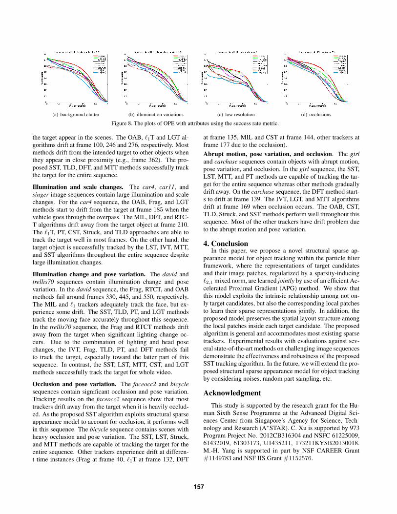
(a) background clutter (b) illumination variations (c) low resolution (d) occlusions

Figure 8. The plots of OPE with attributes using the success rate metric.

the target appear in the scenes. The OAB, ℓ1T and LGT al-

gorithms drift at frame 100, 246 and 276, respectively. Most

methods drift from the intended target to other objects when

they appear in close proximity (e.g., frame 362). The pro-

posed SST, TLD, DFT, and MTT methods successfully track

the target for the entire sequence.

Illumination and scale changes. The car4, car11, and

singer image sequences contain large illumination and scale

changes. For the car4 sequence, the OAB, Frag, and LGT

methods start to drift from the target at frame 185 when the

vehicle goes through the overpass. The MIL, DFT, and RTC-

T algorithms drift away from the target object at frame 210.

The ℓ1T, PT, CST, Struck, and TLD approaches are able to

track the target well in most frames. On the other hand, the

target object is successfully tracked by the LST, IVT, MTT,

and SST algorithms throughout the entire sequence despite

large illumination changes.

Illumination change and pose variation. The david and

trellis70 sequences contain illumination change and pose

variation. In the david sequence, the Frag, RTCT, and OAB

methods fail around frames 330, 445, and 550, respectively.

The MIL and ℓ1 trackers adequately track the face, but ex-

perience some drift. The SST, TLD, PT, and LGT methods

track the moving face accurately throughout this sequence.

In the trellis70 sequence, the Frag and RTCT methods drift

away from the target when significant lighting change oc-

curs. Due to the combination of lighting and head pose

changes, the IVT, Frag, TLD, PT, and DFT methods fail

to track the target, especially toward the latter part of this

sequence. In contrast, the SST, LST, MTT, CST, and LGT

methods successfully track the target for whole video.

Occlusion and pose variation. The faceocc2 and bicycle

sequences contain significant occlusion and pose variation.

Tracking results on the faceocc2 sequence show that most

trackers drift away from the target when it is heavily occlud-

ed. As the proposed SST algorithm exploits structural sparse

appearance model to account for occlusion, it performs well

in this sequence. The bicycle sequence contains scenes with

heavy occlusion and pose variation. The SST, LST, Struck,

and MTT methods are capable of tracking the target for the

entire sequence. Other trackers experience drift at differen-

t time instances (Frag at frame 40, ℓ1T at frame 132, DFT

at frame 135, MIL and CST at frame 144, other trackers at

frame 177 due to the occlusion).

Abrupt motion, pose variation, and occlusion. The girl

and carchase sequences contain objects with abrupt motion,

pose variation, and occlusion. In the girl sequence, the SST,

LST, MTT, and PT methods are capable of tracking the tar-

get for the entire sequence whereas other methods gradually

drift away. On the carchase sequence, the DFT method start-

s to drift at frame 139. The IVT, LGT, and MTT algorithms

drift at frame 169 when occlusion occurs. The OAB, CST,

TLD, Struck, and SST methods perform well throughout this

sequence. Most of the other trackers have drift problem due

to the abrupt motion and pose variation.

4. ConclusionIn this paper, we propose a novel structural sparse ap-

pearance model for object tracking within the particle filter

framework, where the representations of target candidates

and their image patches, regularized by a sparsity-inducing

ℓ2,1 mixed norm, are learned jointly by use of an efficient Ac-

celerated Proximal Gradient (APG) method. We show that

this model exploits the intrinsic relationship among not on-

ly target candidates, but also the corresponding local patches

to learn their sparse representations jointly. In addition, the

proposed model preserves the spatial layout structure among

the local patches inside each target candidate. The proposed

algorithm is general and accommodates most existing sparse

trackers. Experimental results with evaluations against sev-

eral state-of-the-art methods on challenging image sequences

demonstrate the effectiveness and robustness of the proposed

SST tracking algorithm. In the future, we will extend the pro-

posed structural sparse appearance model for object tracking

by considering noises, random part sampling, etc.

Acknowledgment

This study is supported by the research grant for the Hu-

man Sixth Sense Programme at the Advanced Digital Sci-

ences Center from Singapore’s Agency for Science, Tech-

nology and Research (A∗STAR). C. Xu is supported by 973

Program Project No. 2012CB316304 and NSFC 61225009,

61432019, 61303173, U1435211, 173211KYSB20130018.

M.-H. Yang is supported in part by NSF CAREER Grant

#1149783 and NSF IIS Grant #1152576.

157

References

[1] A. Adam, E. Rivlin, and I. Shimshoni. Robust fragments-

based tracking using the integral histogram. In CVPR, pages

798–805, 2006. 1, 5

[2] S. Avidan. Ensemble tracking. In CVPR, pages 494–501,

2005. 1

[3] B. Babenko, M.-H. Yang, and S. Belongie. Visual tracking

with online multiple instance learning. In CVPR, 2009. 1, 5

[4] C. Bao, Y. Wu, H. Ling, and H. Ji. Real time robust l1 track-

er using accelerated proximal gradient approach. In CVPR,

2012. 1, 2, 3, 6

[5] M. J. Black and A. D. Jepson. Eigentracking: Robust match-

ing and tracking of articulated objects using a view-based rep-

resentation. IJCV, pages 63–84, 1998. 1

[6] R. T. Collins and Y. Liu. On-line selection of discriminative

tracking features. In ICCV, pages 346–352, 2003. 1

[7] D. Comaniciu, V. Ramesh, and P. Meer. Kernel-Based Object

Tracking. TPAMI, 25(5):564–575, Apr. 2003. 1

[8] M. Everingham, L. Gool, C. Williams, J. Winn, and A. Zis-

serman. The pascal visual object class (voc) challenge. IJCV,

88(2):303–338, 2010. 6

[9] H. Grabner, M. Grabner, and H. Bischof. Real-Time Tracking

via On-line Boosting. In BMVC, 2006. 1, 5

[10] H. Grabner, C. Leistner, and H. Bischof. Semi-supervised on-

line boosting for robust tracking. In ECCV, 2008. 1

[11] S. Hare, A. Saffari, and P. Torr. Struck: Structured output

tracking with kernels. In ICCV, 2011. 5

[12] J. Henriques, R. Caseiro, P. Martins, and J. Batista. Exploiting

the circulant structure of tracking-by-detection with kernels.

In ECCV, 2012. 5

[13] Z. Hong, X. Mei, D. Prokhorov, and D. Tao. Tracking via

robust multi-task multi-view joint sparse representation. In

ICCV, 2013. 1, 2, 3, 5, 6

[14] A. Jepson, D. Fleet, and T. El-Maraghi. Robust on-line ap-

pearance models for visual tracking. TPAMI, 25(10):1296–

1311, 2003. 1

[15] X. Jia, H. Lu, and M.-H. Yang. Visual tracking via adaptive

structural local sparse appearance model. In CVPR, 2012. 1,

2, 3, 4, 5, 6

[16] Z. Kalal, J. Matas, and K. Mikolajczyk. P-N Learning: Boot-

strapping Binary Classifiers by Structural Constraints. In

CVPR, 2010. 1, 5

[17] M. Kristan, L. Cehovin, and et al. The visual object tracking

vot 2013 challenge results. In ICCV2013 Workshops, Work-

shop on Visual Object Tracking Challenge, 2013. 1

[18] J. Kwon and K. M. Lee. Visual tracking decomposition. In

CVPR, 2010. 1

[19] H. Li, C. Shen, and Q. Shi. Real-time visual tracking with

compressed sensing. In CVPR, 2011. 1, 2, 3, 5

[20] B. Liu, J. Huang, L. Yang, and C. Kulikowski. Robust visual

tracking with local sparse appearance model and k-selection.

In CVPR, 2011. 1, 2, 3, 4, 5

[21] B. Liu, L. Yang, J. Huang, P. Meer, L. Gong, and C. Kulikows-

ki. Robust and fast collaborative tracking with two stage s-

parse optimization. In ECCV, 2010. 1, 2, 3, 5

[22] X. Mei and H. Ling. Robust Visual Tracking and Vehicle Clas-

sification via Sparse Representation. TPAMI, 33(11):2259–

2272, 2011. 1, 2, 3, 4, 5, 6

[23] X. Mei, H. Ling, Y. Wu, E. Blasch, and L. Bai. Minimum

error bounded efficient l1 tracker with occlusion detection. In

CVPR, 2011. 1, 2, 3, 5, 6

[24] Y. Pang and H. Ling. Finding the best from the second best-

s - inhibiting subjective bias in evaluation of visual tracking

algorithms. In ICCV, 2013. 1

[25] D. Ross, J. Lim, R.-S. Lin, and M.-H. Yang. Incremental

Learning for Robust Visual Tracking. IJCV, 77(1):125–141,

2008. 1, 5

[26] S. Salti, A. Cavallaro, and L. D. Stefano. Adaptive appear-

ance modeling for video tracking: Survey and evaluation. TIP,

21(10):4334–4348, 2012. 1

[27] L. Sevilla-Lara and E. Learned-Miller. Distribution fields for

tracking. In CVPR, pages 1910–1917, 2012. 5

[28] L. Cehovin, M. Kristan, and A. Leonardis. Robust visual

tracking using an adaptive coupled-layer visual model. TPA-

MI, 35(4):941–953, 2013. 5

[29] D. Wang, H. Lu, and M. Yang. Online Object Tracking with

Sparse Prototypes. IEEE Transaction on Image Processing,

22(1):314–325, 2013. 1

[30] Y. Wu, J. Lim, and M.-H. Yang. Online object tracking: A

benchmark. In CVPR, 2013. 1, 6

[31] M. Yang, Y. Wu, and G. Hua. Context-aware visual tracking.

TPAMI, 31(7):1195–1209, 2009. 1

[32] R. Yao, Q. Shi, C. Shen, Y. Zhang, and A. van den Hengel.

Part-based visual tracking with online latent structural learn-

ing. In CVPR, 2013. 5

[33] A. Yilmaz, O. Javed, and M. Shah. Object tracking: A survey.

ACM Comput. Surv., 38(4):13, Dec. 2006. 1

[34] K. Zhang, L. Zhang, and M.-H. Yang. Real-time compressive

tracking. In ECCV, 2012. 1, 2, 3, 5, 6

[35] T. Zhang, B. Ghanem, and N. Ahuja. Robust multi-object

tracking via cross-domain contextual information for sport-

s video analysis. In International Conference on Acoustics,

Speech and Signal Processing, 2012. 1

[36] T. Zhang, B. Ghanem, S. Liu, and N. Ahuja. Low-rank sparse

learning for robust visual tracking. In ECCV, 2012. 1, 2, 3, 5

[37] T. Zhang, B. Ghanem, S. Liu, and N. Ahuja. Robust visual

tracking via multi-task sparse learning. In CVPR, 2012. 1, 2,

3, 5, 6

[38] T. Zhang, B. Ghanem, S. Liu, and N. Ahuja. Robust visual

tracking via structured multi-task sparse learning. Interna-

tional Journal of Computer Vision, 101(2):367–383, 2013. 3

[39] T. Zhang, C. Jia, C. Xu, Y. Ma, and N. Ahuja. Partial occlu-

sion handling for visual tracking via robust part matching. In

CVPR, 2014. 1

[40] T. Zhang, S. Liu, N. Ahuja, M.-H. Yang, and B. Ghanem. Ro-

bust Visual Tracking via Consistent Low-Rank Sparse Learn-

ing. International Journal of Computer Vision, 111(2):171–

190, 2015. 3

[41] W. Zhong, H. Lu, and M. Yang. Robust Object Tracking via

Sparse Collaborative Appearance Model. IEEE Transaction

on Image Processing, 23(5):2356–2368, 2014. 1

[42] B. Zhuang, H. Lu, Z. Xiao, and D. Wang. Visual Tracking via

Discriminative Sparse Similarity Map. IEEE Transaction on

Image Processing, 23(4):1872–1881, 2014. 1

158