Structural Stochastic Volatility in Asset Pricing Dynamics: Estimation and Model Contest Reiner Franke Frank Westerhoff Working Paper No. 78 April 2011 k* b 0 k B A M AMBERG CONOMIC ESEARCH ROUP B E R G Working Paper Series BERG on Government and Growth Bamberg Economic Research Group on Government and Growth Bamberg University Feldkirchenstraße 21 D-96045 Bamberg Telefax: (0951) 863 5547 Telephone: (0951) 863 2547 E-mail: [email protected]http://www.uni-bamberg.de/vwl-fiwi/forschung/berg/ ISBN 978-3-931052-88-1
Transcript
Structural Stochastic Volatility in Asset Pricing Dynamics:
Estimation and Model Contest
Reiner Franke
Frank Westerhoff
Working Paper No. 78
April 2011
k*
b
0 k
BA
MAMBERG
CONOMIC
ESEARCH
ROUP
BE
RG
Working Paper SeriesBERG
on Government and Growth
Bamberg Economic Research Group
on Government and Growth Bamberg University Feldkirchenstraße 21 D-96045 Bamberg
Structural Stochastic Volatility in Asset Pricing Dynamics:
Estimation and Model Contest
Reiner Franke aFrank Westerhoff b,∗
February 2011
aUniversity of Kiel, GermanybUniversity of Bamberg, Germany
Abstract
In the framework of small-scale agent-based financial market models, the paper startsout from the concept of structural stochastic volatility, which derives from different noiselevels in the demand of fundamentalists and chartists and the time-varying market sharesof the two groups. It advances several different specifications of the endogenous switchingbetween the trading strategies and then estimates these models by the method of simu-lated moments (MSM), where the choice of the moments reflects the basic stylized factsof the daily returns of a stock market index. In addition to the standard version of MSMwith a quadratic loss function, we also take into account how often a great number ofMonte Carlo simulation runs happen to yield moments that are all contained within theirempirical confidence intervals. The model contest along these lines reveals a strong rolefor a (tamed) herding component. The quantitative performance of the winner model isso good that it may provide a standard for future research.
JEL classification: D84; G12; G14; G15.
Keywords: Method of simulated moments; moment coverage ratio; herding; discretechoice approach; transition probability approach.
1. Introduction
Over the past ten or twenty years, a rich literature on small-scale asset pricing models hascome into bloom that abandon the rational expectations framework and rather considerthe financial markets as being populated by a few groups of agents who rely on simpleheuristic trading strategies. 1 Currently numerical simulations tend to become the rule.
1 Recent surveys on this research are Hommes (2006), LeBaron (2006), Chiarella et al. (2009),Lux (2009) and Westerhoff (2009), among others.
They do not only illustrate the basic mechanisms but also attempt to match certainstylized facts in quantitative ways. Contributing to this research, the present paper hasthree main goals: (1) the specification of different versions of a promising modellingapproach featuring what we call structural stochastic volatility; (2) the estimation ofthese models on daily returns from a major stock market index; and (3) a competitivecomparison of the estimation results.
Let us begin with a brief characterization of the concept of structural stochastic volatil-ity. The most elementary form in which we model it here is based on the usual archetypesof financial markets participants, i.e. chartists who extrapolate past price trends and fun-damentalists who bet on mean reversion. However, the asset demand of the two types ofagents is noisy and the corresponding noise levels may also be different. If then the marketshares of fundamentalists and chartists are varying over time, the overall noise level in thedemand-induced price changes will be varying, too. In addition, a dominance of chart-ists favours the emergence of bubbles and a dominance of fundamentalists is conduciveto more tranquil market periods. In this way there is scope for the returns to exhibitstochastic volatility. In contrast to the technical GARCH models and their refinements,this phenomenon has now a structural, although parsimonious, underpinning.
To make this general idea workable, we next have to ask what governs the endoge-nous switches between the two trading strategies. Four socio-economic principles will beconsidered in this respect: (a) predisposition as a behavioural bias towards one of thetrading strategies; (b) differential wealth that hypothetically would have been earned bythe two strategies over the past (making a strategy more attractive the more successfulit has been); (c) herding, which means that the attractiveness of a group rises with theshare it already has in the total population; (d) a misalignment correction mechanism,according to which high deviations of the price from its fundamental value increase thefears that the bubble will eventually burst and, as a result, fundamentalism is expectedto become more profitable again.
Choosing in various ways from this set, the single mechanisms are additively combinedin a switching index which summarizes the relative attractiveness of fundamentalismversus chartism. The models are then completed by incorporating the index into one oftwo different devices. The first one is the well-known discrete choice approach along thelines of Brock and Hommes (1997), where the switching index determines the fractionsof the two groups of traders directly by a nonlinear functional relationship. In the otherapproach, which goes back to Weidlich and Haag (1983) and Lux (1995), the switchingindex influences the probabilities with which the agents switch to the opposite group.In the aggregate it is here the change of the market fractions that is determined by theindex. On the whole, seven model variants will be studied in greater detail.
While until a few years ago researchers have contended themselves with calibratingtheir models in informal ways, there are now a number of attempts to estimate them in
2
a more systematic manner. 2 A most suitable approach for the present kind of modelsis the method of simulated moments (MSM), where ‘moments’ refers to the time seriesof one or several variables and means certain summary statistics of them. In the presentcontext they should reflect what is considered to be the most important stylized facts ofthe daily stock market returns, in particular, volatility clustering and fat tails.
In pursuing the second goal of the paper, we first follow the standard specificationof MSM. It searches for the parameter values of a model that minimize the distancebetween the empirical and simulated, i.e. model-generated moments, where the distanceis defined by a quadratic loss function. In addition, we will introduce the joint momentcoverage ratio (MCR) as an alternative evaluation criterion. This is the percentage ratioof a great number of simulation runs of the model the moments of which are all containedwithin their empirical confidence intervals. Since the models are thus required to matchnine (rather diverse) moments, a ratio of more than five per cent, say, would already bequite an achievement.
After the ground has thus been prepared, we can turn to the third goal of the paperand ask the most obvious question: which of our models is the best? In particular, we findout here that the two estimation criteria, although being similar in spirit, convey differentinformation, so that even the ranking of the models may be affected. As a consequence,we estimate the models for each criterion separately. To anticipate the answer to ourquestion, in both cases the winner is the discrete choice model that includes herding,predisposition, and the misalignment effect. Defining a (moment-specific) bootstrappedp-value to quantify a model’s goodness-of-fit, it turns out that roughly one-third of allsimulation runs cannot be directly rejected by the data. On the other hand, the jointMCR amounts to more than 25 per cent, which we think is a fairly respectable order ofmagnitude as well.
It is furthermore remarkable that both estimation procedures also yield the samemodel in second place. This is the model that incorporates the same three effects intothe transition probability approach. We learn from this result that what makes the notionof structural stochastic volatility most successful is an appropriate choice of the socio-economic principles governing the switching between the two trading strategies, whereasthe differences between the discrete choice and transition probability approach seem tobe of second order importance.
The remainder of the paper is organized as follows. Section 2 reiterates the constituentparts of the method of simulated moments and specifies the set of moments that will beunderlying the estimations. Section 3 presents the model variants that we select for esti-mation. It is here also illustrated that they can give rise to rather different patterns of theswitching between chartism and fundamentalism. The estimation results and their com-
2 See Gilli and Winker (2003), Alfarano et al. (2005), Manzan and Westerhoff (2007), Winkeret al. (2007), Amilon (2008), Franke (2009), Li et al. (2010), Chiarella et al. (2011), Franke andWesterhoff (2011).
3
prehensive discussion are contained in Section 4. Section 5 concludes, and an appendixdetails the computation of the confidence intervals of the empirical moments.
2. The method of simulated moments
2.1. The standard objective function
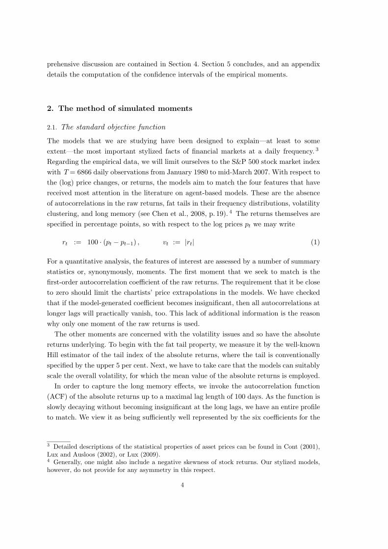
The models that we are studying have been designed to explain—at least to someextent—the most important stylized facts of financial markets at a daily frequency. 3
Regarding the empirical data, we will limit ourselves to the S&P 500 stock market indexwith T = 6866 daily observations from January 1980 to mid-March 2007. With respect tothe (log) price changes, or returns, the models aim to match the four features that havereceived most attention in the literature on agent-based models. These are the absenceof autocorrelations in the raw returns, fat tails in their frequency distributions, volatilityclustering, and long memory (see Chen et al., 2008, p. 19). 4 The returns themselves arespecified in percentage points, so with respect to the log prices pt we may write
rt := 100 · (pt − pt−1) , vt := |rt| (1)
For a quantitative analysis, the features of interest are assessed by a number of summarystatistics or, synonymously, moments. The first moment that we seek to match is thefirst-order autocorrelation coefficient of the raw returns. The requirement that it be closeto zero should limit the chartists’ price extrapolations in the models. We have checkedthat if the model-generated coefficient becomes insignificant, then all autocorrelations atlonger lags will practically vanish, too. This lack of additional information is the reasonwhy only one moment of the raw returns is used.
The other moments are concerned with the volatility issues and so have the absolutereturns underlying. To begin with the fat tail property, we measure it by the well-knownHill estimator of the tail index of the absolute returns, where the tail is conventionallyspecified by the upper 5 per cent. Next, we have to take care that the models can suitablyscale the overall volatility, for which the mean value of the absolute returns is employed.
In order to capture the long memory effects, we invoke the autocorrelation function(ACF) of the absolute returns up to a maximal lag length of 100 days. As the function isslowly decaying without becoming insignificant at the long lags, we have an entire profileto match. We view it as being sufficiently well represented by the six coefficients for the
3 Detailed descriptions of the statistical properties of asset prices can be found in Cont (2001),Lux and Ausloos (2002), or Lux (2009).4 Generally, one might also include a negative skewness of stock returns. Our stylized models,however, do not provide for any asymmetry in this respect.
4
lags 1, 5, 10, 25, 50, 100. To reduce the influence of accidental outlier effects that mightjust show up at one of the selected lags, the centred three-lag averages are computed. 5
The performance of our models is evaluated on the basis of these nine moments, whichwe summarize in a (column) vector m = (m1, . . . , m9)′ (the prime denotes transposition).They are to come close to their empirical counterparts, which may be designated memp
(the values of the latter can be found in Table A1 in the Appendix). The distancebetween m and memp is defined by a quadratic function with a suitable weighting matrixW ∈ IR9×9 (to be specified shortly). We thus have the following loss function for themodel-generated (and other) moments,
J = J(m) := (m−memp)′ W (m−memp) (2)
In the first instance, this function serves to estimate a model by the method of simu-lated moments (MSM). To this end, it is simulated over S periods, or days (after aninitial period of several hundred days is discarded to rule out any transitory effects).The simulations are repeated for alternative sets of the structural parameters of themodel, and estimation means to minimize the associated loss. It goes here without say-ing that for each parameter set the same random number sequence is used. 6 Collectingthe parameters to be estimated in a vector θ and denoting the moments from the corre-sponding simulations by m = m(θ;S), MSM therefore amounts to solving the followingminimization problem,
J [m(θ;S)] = minθ
! (3)
To reduce the sample variability in the stochastic simulations, the time horizon is chosenlonger than the empirical sample period T . As it is common practice, we will work withS = 10 · T . It would furthermore be possible to determine the asymptotic standarderrors of the parameter estimates. Since the main focus of this paper is on the fittingproperties of alternative models, we will, however, leave the issue of the precision of ourestimates aside. Suffice it to note that all of the parameter values that we will report aresignificantly different from zero.
2.2. The weighting matrix
The weighting matrix W in the objective function J takes the sampling variability ofthe moments into account. The basic idea is that the higher the sampling variability
5 That is, at lag τ the mean of the three autocorrelation coefficients for τ−1, τ , τ+1 is computed,except for τ = 1, where it is the average of the first and second coefficient. It may also be notedthat volatility clustering, which describes the tendency of large changes in the asset price to befollowed by large changes, and small changes to be followed by small changes, is closely relatedto these long-range dependencies between the returns.6 Entering the models will be normally distributed random terms εt with variance σ2
t . Identicalrandom number sequences then mean that for each simulation run at time t the same randomnumber εt is drawn from the standard normal distribution N(0, 1), and εt is subsequently obtainedas σt εt.
5
of a given moment i, the larger the differences between mi and mempi that can still be
deemed insignificant. This can primarily be achieved by a correspondingly small diagonalelement wii. In addition, the matrix W should provide for possible correlations betweenthe single moments. An obvious candidate for a suitable weighting matrix is the inverseof an estimated variance-covariance matrix Σ of the moments,
W = Σ−1
(4)
One such estimate Σ to set up W may be obtained from a Newey-West estimator of thelong-run covariance matrix of the empirical moments (see, e.g., Lee and Ingram, 1991,p. 202, or the application of MSM in Franke, 2009, Section 2.2). In this paper, we followWinker et al. (2007) and Franke and Westerhoff (2010) and choose a bootstrap approachto construct from the empirical data a large number of samples of the moments, fromwhich subsequently the covariances can be derived.
More exactly, a block bootstrap is appropriate due to the long-range dependence inthe return series. An immediate idea for choosing the block length is one year, i.e. 250days. Thus we reduce our empirical return series of S&P 500 (which comprises 6866 datapoints) to T ′ = 6750 observations, subdivide it into 27 fixed and non-overlapping blocksof 250 days, and construct a new series, block by block, from 27 random draws (withreplacement). All of the desired moments can then be computed from this string of theblocks of returns.
Repeating this procedure 5000 times, a frequency distribution for each of the momentsis obtained. Ideally, the empirical moment should be more or less in the centre of thedistribution. For the ACF of the absolute returns at longer lags τ ≥ 10, however, thebootstrapped coefficients show a non-negligible tendency towards lower values. It wasfound that the bias is appreciably mitigated by using longer blocks of 500 and 750 days. 7
Following the conclusions that have already been drawn in Franke and Westerhoff (2010,Section 3), we choose a block length of 250 days for the first five “short memory” moments(first-order autocorrelation of the raw returns and with respect to the absolute returns,the Hill estimator, mean volatility and the autocorrelations at lags τ = 1 and τ = 5),and a block length of 750 days for the last four “long memory” moments (the ACF ofvt = |rt| at lags τ = 10, 25, 50, 100).
The frequency distributions of these bootstrapped moments are taken to obtain an es-timate Σ of the moments’ variance-covariance matrix. Formally, let b = 1, . . . , B identifythe bootstrap samples (B = 5000 presently), let mb = (mb
1, . . . , mb9)′ be the resulting
moment vectors, and compute the vector of their mean values m: := (1/B)∑
b mb. Fromthis, Σ results like
Σ :=1B
B∑b=1
(mb − m:)(mb − m:)′ (5)
7 Unfortunately, blocks of 1000 days seem too long compared to the empirical sample period.
6
To sum up, the models that will be introduced in the next section are estimated byminimizing the objective function J in (3), where J is defined by eqs (2), (4), (5) and ofcourse the set of the nine moments described in the text.
The minimization is carried out by means of the Nelder-Mead simplex algorithm (seePress et al., 1986, pp. 289–293). To avoid getting prematurely trapped in a local mini-mum, the procedure is several times restarted with a relatively large new initial simplexwhich hopefully reaches beyond the “hills” surrounding a local “valley”, until no furthernoteworthy improvement in the minimization occurs. If in the course of the search someparameter violates a non-negativity constraint and becomes negative, we reset it to zeroto run the simulation. However, after computing J from its moments, a penalty is addedthat proportionately increases with the extent of the violation. Taking all this into ac-count, we are fairly confident for each of the estimations that, given the random numberseed, the search algorithm has led us sufficiently close to a global minimum.
3. Alternative switching mechanisms to get structural stochasticvolatility
3.1. The common model building blocks of demand and its price impact
The two groups of fundamentalist and chartist traders, their specification of demandfor the asset, and the impact of aggregate demand on the price are common to all ofthe model versions that we consider. 8 To begin with the latter, the market is generallyallowed to be in disequilibrium. A market maker is assumed to hold inventory, fromwhich he serves any excess of demand and to which he puts any excess of supply. Hereacts to this imbalance by proportionately adjusting the price for the next period witha (constant) factor µ > 0 in the direction of excess demand. Thus, letting pt be the(log) price that he quotes at the beginning of period t, df
t−1 and dct−1 the demand in the
previous period of an average fundamentalist and chartist trader, respectively, and nft−1,
nct−1 the market fractions of the two groups in that period, the price impact equation
reads,
pt = pt−1 + µ (nft−1 df
t−1 + nct−1 dc
t−1) (6)
Regarding the formulation of demand, we join numerous examples in the literature and,in the first step, postulate two extremely simple deterministic rules. They govern what wemay call the core demand of an average trader in each group. For the fundamentalists,this demand is inversely related to the deviations of the price from its fundamentalvalue. That is, in period t it is proportional to the gap (p? − pt), p? being the (log ofthe) fundamental value, which we treat as an exogenously given constant (for simplicity
8 To be exact, by demand we mean the orders (positive or negative) per trading period, not thedesired positions of the agents.
7
and to show that no random walk behaviour of the fundamental value is required toobtain the stylized facts). The core demand of the group of chartists is hypothesized tobe proportional to the returns they have just observed, i.e. (pt − pt−1).
A crucial feature of our models is that we add a noise term to each of these demandcomponents (and not just their sum). The two terms are supposed to reflect a certainwithin-group heterogeneity, which we do not wish to describe in full detail. Since the manyindividual digressions from the simple rules as well as their composition in each groupwill more or less accidentally fluctuate from period to period, it is a natural short-cut tohave this heterogeneity represented by two independent and normally distributed randomvariables εf
t and εct for the fundamentalists and chartists, respectively. 9 Combining the
deterministic and stochastic elements, the net demands of the average fundamentalistand chartist trader for the asset in period t are given by
dft = φ (p? − pt) + εf
t , εft ∼ N(0, σ2
f ) (7)
dct = χ (pt − pt−1) + εc
t , εct ∼ N(0, σ2
c ) (8)
where here and in the following, the Greek symbols denote constant and nonnegativeparameters.
Plugging (7) and (8) into the price impact function (6), we do get one single noiseterm acting on the price changes, or returns (as the sum of two normal distributions).Its variance σ2
t is, however, dependent on the variations of the market fractions of thefundamentalists and chartists, σ2
t = (nft−1)
2 σ2f +(nc
t−1)2 σ2
c , even if the two group-specificvariances σ2
f and σ2c were equal. This feature of a time-varying variance in the returns is
what was coined structural stochastic volatility (SSV) in Franke and Westerhoff (2009).Nevertheless, whether in this way also the most important stylized fact of the returns canbe matched by the model will, in the first instance, be a matter of the specific switchingmechanisms between the two groups of traders. A number of different proposals for themwill be introduced next.
3.2. The transition probability and discrete choice approaches
There are two by now fairly standard formulations in the literature that specify howthe agents in a simple model may switch between two or more attitudes, or groups: thetransition probability approach and the discrete choice approach. For easier reference wemay also use the acronyms TPA and DCA, respectively.
9 For example, individual and presently active traders with a fundamentalist strategy may adoptdifferent values for their fundamental price, they react with different intensities to their tradingsignal, or they experiment with more complex trading rules which may also be continuouslysubjected to further modifications. Similarly so for the chartists, which explains the independenceof εf
t and εct . In short, the two noise variables can be conceived of as a most convenient short-cut
of certain aspects that are more specifically dealt with in models with hundreds or thousandsof different agents that one would have to keep track of over time (see Farmer and Joshi, 2002;LeBaron, 2006).
8
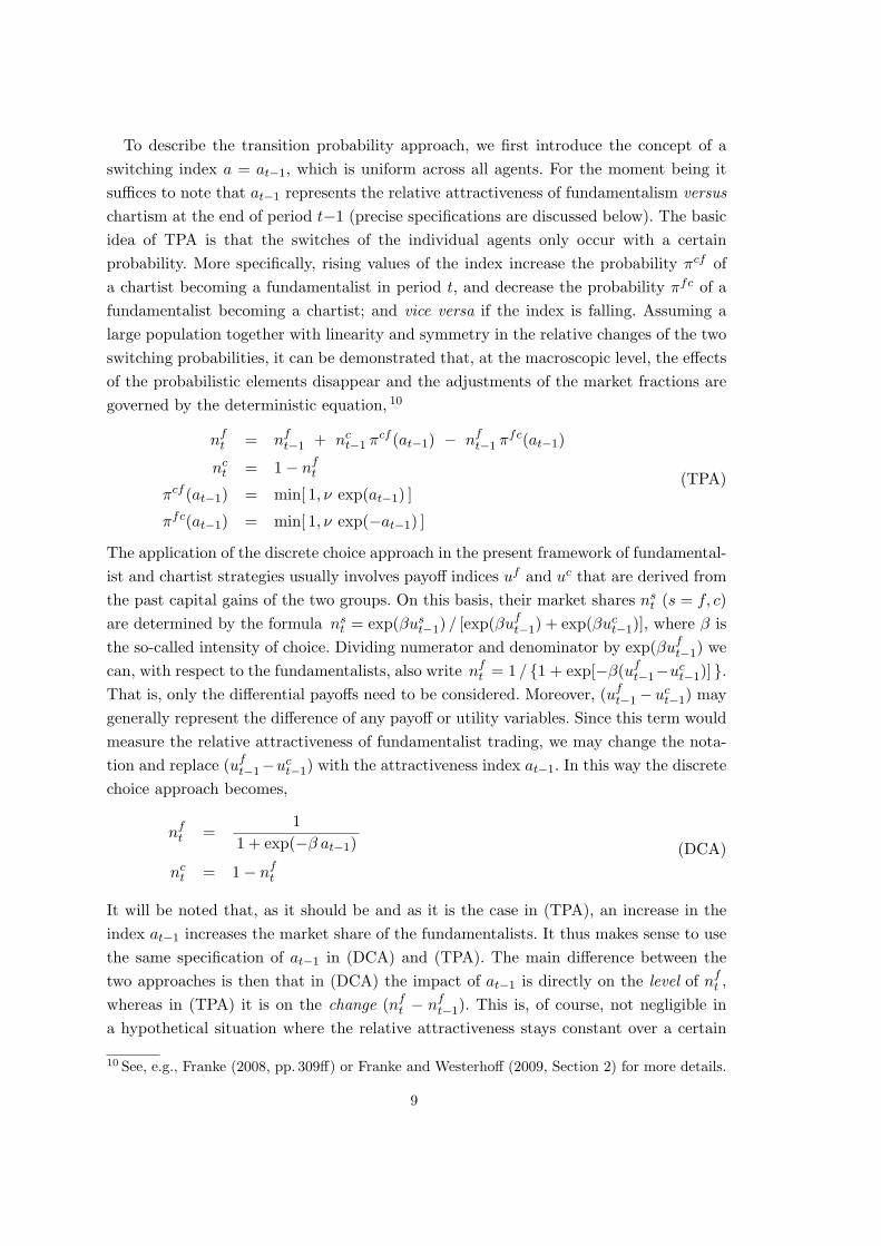
To describe the transition probability approach, we first introduce the concept of aswitching index a = at−1, which is uniform across all agents. For the moment being itsuffices to note that at−1 represents the relative attractiveness of fundamentalism versuschartism at the end of period t−1 (precise specifications are discussed below). The basicidea of TPA is that the switches of the individual agents only occur with a certainprobability. More specifically, rising values of the index increase the probability πcf ofa chartist becoming a fundamentalist in period t, and decrease the probability πfc of afundamentalist becoming a chartist; and vice versa if the index is falling. Assuming alarge population together with linearity and symmetry in the relative changes of the twoswitching probabilities, it can be demonstrated that, at the macroscopic level, the effectsof the probabilistic elements disappear and the adjustments of the market fractions aregoverned by the deterministic equation, 10
nft = nf
t−1 + nct−1 πcf (at−1) − nf
t−1 πfc(at−1)
nct = 1− nf
t
πcf (at−1) = min[ 1, ν exp(at−1) ]
πfc(at−1) = min[ 1, ν exp(−at−1) ]
(TPA)
The application of the discrete choice approach in the present framework of fundamental-ist and chartist strategies usually involves payoff indices uf and uc that are derived fromthe past capital gains of the two groups. On this basis, their market shares ns
t (s = f, c)are determined by the formula ns
t = exp(βust−1) / [exp(βuf
t−1) + exp(βuct−1)], where β is
the so-called intensity of choice. Dividing numerator and denominator by exp(βuft−1) we
can, with respect to the fundamentalists, also write nft = 1 / {1 + exp[−β(uf
t−1−uct−1)] }.
That is, only the differential payoffs need to be considered. Moreover, (uft−1− uc
t−1) maygenerally represent the difference of any payoff or utility variables. Since this term wouldmeasure the relative attractiveness of fundamentalist trading, we may change the nota-tion and replace (uf
t−1−uct−1) with the attractiveness index at−1. In this way the discrete
choice approach becomes,
nft =
11 + exp(−β at−1)
nct = 1− nf
t
(DCA)
It will be noted that, as it should be and as it is the case in (TPA), an increase in theindex at−1 increases the market share of the fundamentalists. It thus makes sense to usethe same specification of at−1 in (DCA) and (TPA). The main difference between thetwo approaches is then that in (DCA) the impact of at−1 is directly on the level of nf
t ,whereas in (TPA) it is on the change (nf
t − nft−1). This is, of course, not negligible in
a hypothetical situation where the relative attractiveness stays constant over a certain
10 See, e.g., Franke (2008, pp. 309ff) or Franke and Westerhoff (2009, Section 2) for more details.
9
period of time. On the other hand, in the fully dynamic models with the endogenousdeterministic and stochastic interactions of the variables, the differences might possiblybe less substantial, provided that some of the parameters are suitably adjusted. This isindeed an important topic that we will have an eye on in the estimations below.
3.3. Specification of the relative attractiveness
We consider four principles that may play a role in the agents’ choice of one of the twostrategies, which as we have seen is tantamount to the determination of the relativeattractiveness. Correspondingly, we put forward four components some of which, in var-ious combinations, are added to yield the level of attractiveness at at the end of period t.The first principle is herding (H), which means that joining a group becomes the moreattractive the more adherents it already has. This idea is straightforwardly representedby a term that is proportional to the most recent difference (nf
t − nct) between the two
market fractions.The second principle is based on the abovementioned differential profits, where the
modelling literature usually incorporates some inertia. 11 With respect to strategy s =f, c, let to this end gs
t be the short-term capital gains that an average agent in thisgroup could realize at day t. They derive from the (average) demand formulated at t−2and executed at the price pt−1 of the following day. Furthermore, let us
t be the ‘utility’obtained from these capital gains and η a memory coefficient between zero and one. Thespecification then typically reads us
t = gst + η us
t−1. We follow the same idea but considerit more meaningful to have a weighted average of gs
t and ust−1 on the right-hand side of
this equation. So we work with
gst = [exp(pt)− exp(pt−1)] ds
t−2 ,
wst = η ws
t−1 + (1−η) gst ,
s = c, f (9)
The reason for our slight modification and for replacing the symbol u with w is theinterpretation to which (9) gives rise. In fact, the second equation in (9) is equivalent tothe infinite sum
wst = (1− η)
∞∑k=0
ηk gst−k
Apart from the rescaling by (1−η), wst therefore represents the accumulated profits,
discounted by the coefficient η<1, that would have been earned by a hypothetical agentwho consistently had followed strategy s over the infinite past on a day-to-day basis. Inother words, ws is the hypothetical wealth attributable to strategy s. Equipped with the
11 Occasionally, reference is also made to the squared forecast errors of the agents (in Brock andDe Fontnouvelle, 2000, for example). We view this as a more indirect specification of differentialprofits (which would derive from them) and neglect it to limit our investigations.
10
concept of eq. (9), the second component determining at is proportional to the difference(wf
t − wct ). This feature may be identified by the letter (W).
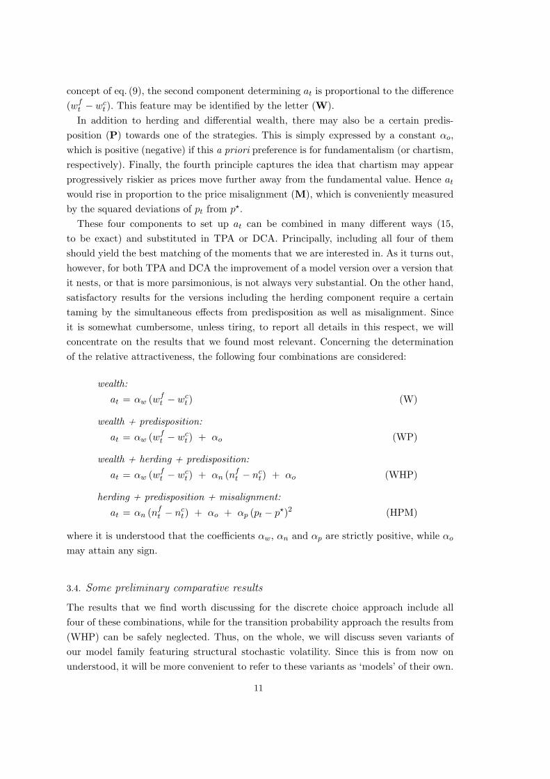
In addition to herding and differential wealth, there may also be a certain predis-position (P) towards one of the strategies. This is simply expressed by a constant αo,which is positive (negative) if this a priori preference is for fundamentalism (or chartism,respectively). Finally, the fourth principle captures the idea that chartism may appearprogressively riskier as prices move further away from the fundamental value. Hence at
would rise in proportion to the price misalignment (M), which is conveniently measuredby the squared deviations of pt from p?.
These four components to set up at can be combined in many different ways (15,to be exact) and substituted in TPA or DCA. Principally, including all four of themshould yield the best matching of the moments that we are interested in. As it turns out,however, for both TPA and DCA the improvement of a model version over a version thatit nests, or that is more parsimonious, is not always very substantial. On the other hand,satisfactory results for the versions including the herding component require a certaintaming by the simultaneous effects from predisposition as well as misalignment. Sinceit is somewhat cumbersome, unless tiring, to report all details in this respect, we willconcentrate on the results that we found most relevant. Concerning the determinationof the relative attractiveness, the following four combinations are considered:
wealth:
at = αw (wft − wc
t ) (W)
wealth + predisposition:
at = αw (wft − wc
t ) + αo (WP)
wealth + herding + predisposition:
at = αw (wft − wc
t ) + αn (nft − nc
t) + αo (WHP)
herding + predisposition + misalignment:
at = αn (nft − nc
t) + αo + αp (pt − p?)2 (HPM)
where it is understood that the coefficients αw, αn and αp are strictly positive, while αo
may attain any sign.
3.4. Some preliminary comparative results
The results that we find worth discussing for the discrete choice approach include allfour of these combinations, while for the transition probability approach the results from(WHP) can be safely neglected. Thus, on the whole, we will discuss seven variants ofour model family featuring structural stochastic volatility. Since this is from now onunderstood, it will be more convenient to refer to these variants as ‘models’ of their own.
11
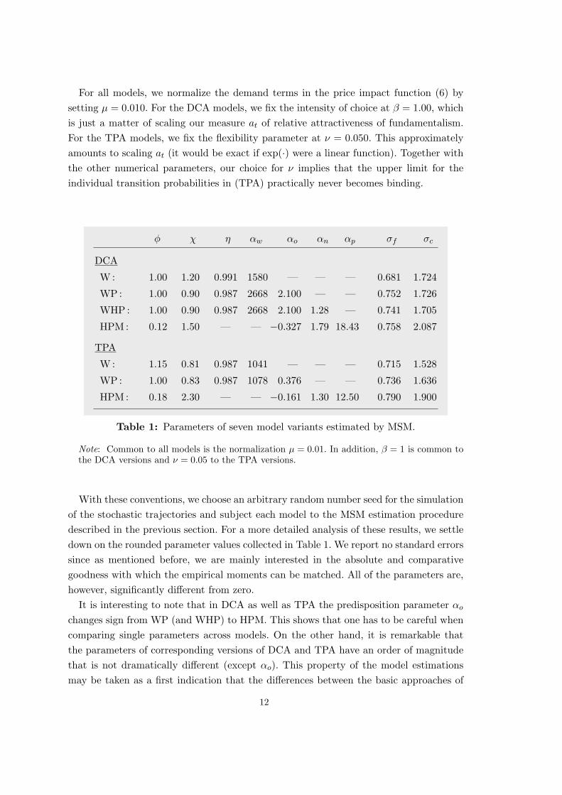
For all models, we normalize the demand terms in the price impact function (6) bysetting µ = 0.010. For the DCA models, we fix the intensity of choice at β = 1.00, whichis just a matter of scaling our measure at of relative attractiveness of fundamentalism.For the TPA models, we fix the flexibility parameter at ν = 0.050. This approximatelyamounts to scaling at (it would be exact if exp(·) were a linear function). Together withthe other numerical parameters, our choice for ν implies that the upper limit for theindividual transition probabilities in (TPA) practically never becomes binding.
Table 1: Parameters of seven model variants estimated by MSM.
Note: Common to all models is the normalization µ = 0.01. In addition, β = 1 is common tothe DCA versions and ν = 0.05 to the TPA versions.
With these conventions, we choose an arbitrary random number seed for the simulationof the stochastic trajectories and subject each model to the MSM estimation proceduredescribed in the previous section. For a more detailed analysis of these results, we settledown on the rounded parameter values collected in Table 1. We report no standard errorssince as mentioned before, we are mainly interested in the absolute and comparativegoodness with which the empirical moments can be matched. All of the parameters are,however, significantly different from zero.
It is interesting to note that in DCA as well as TPA the predisposition parameter αo
changes sign from WP (and WHP) to HPM. This shows that one has to be careful whencomparing single parameters across models. On the other hand, it is remarkable thatthe parameters of corresponding versions of DCA and TPA have an order of magnitudethat is not dramatically different (except αo). This property of the model estimationsmay be taken as a first indication that the differences between the basic approaches of
12
DCA and TPA are less important than different specifications of the index of relativeattractiveness itself.
Figure 1 presents sample runs of four models over 7000 periods, i.e. 7000 days. Thecomparison of the evolution of the market fraction of chartists illustrates that the modelscan give rise to fairly different patterns of the switching between chartism and funda-mentalism, although the random number sequences in the demand terms are identical.The smallest differences are observed between the most elementary versions of DCA andTPA, when only the wealth effect enters the determination of the relative attractiveness.On the whole, they produce rather similar movements of nc
t , but DCA exhibits morevariability over shorter periods of time.
Figure 1: Market fraction of chartists in four model variants.
The distinguishing feature of the two DCA models in the upper two panels in Figure1 is a positive predisposition of the agents towards fundamentalism in DCA–WP. Sincethe other parameter values are not very different, the latter model has on average alower weight of the chartists in the market. For example, we have a similarly pronouncedchartist regime around t = 5000 in the two models, but it sooner and more dramatically
13
breaks down in DCA–WP. Nevertheless, the overall noise level of nct seems to be about
the same.The bottom panel in the figure is another indication that the main differences between
the model versions are not so much to be sought in the two approaches of discrete choiceand the transition probabilities, but whether in the determination of the index of relativeattractiveness herding is present or not. In fact, the TPA–HPM model shows very fewepisodes of a chartist regime, and also otherwise chartists have a very low weight in themarket.
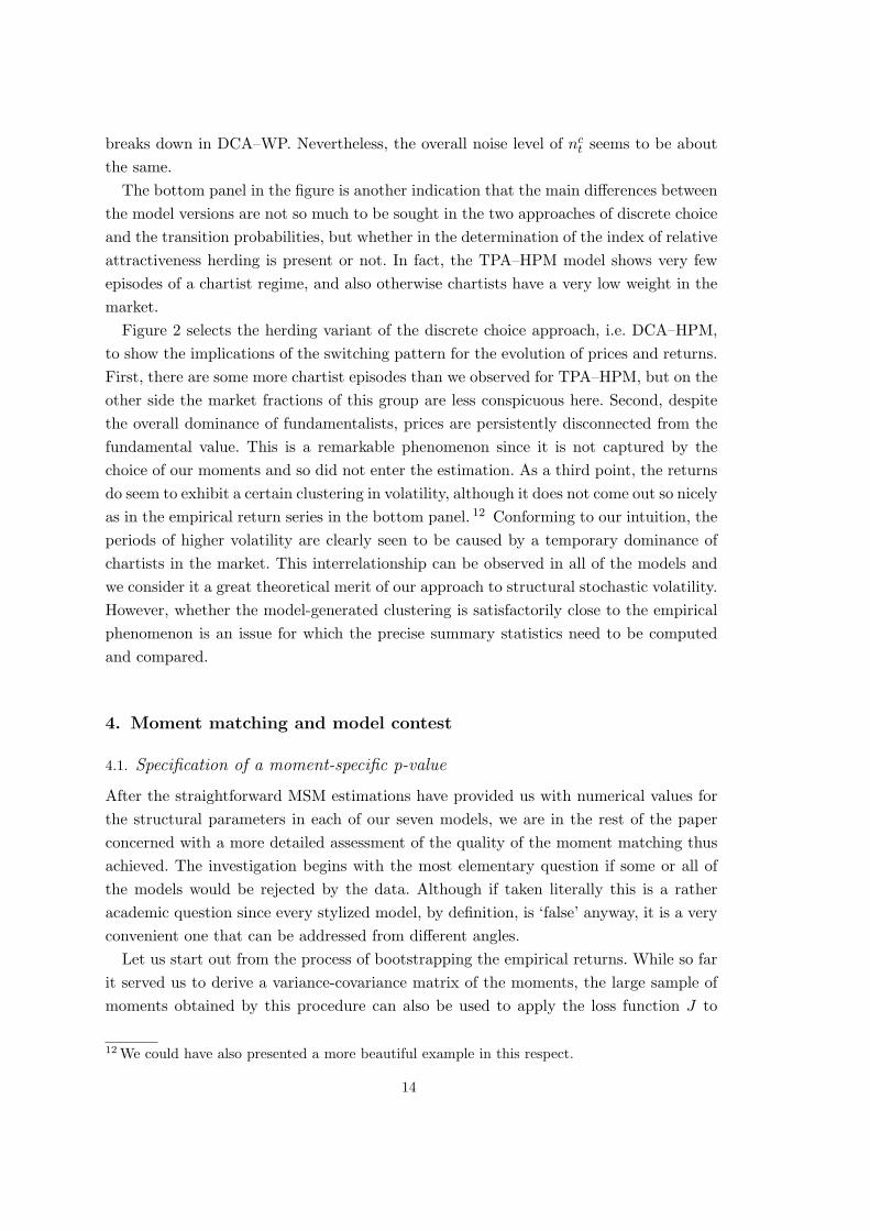
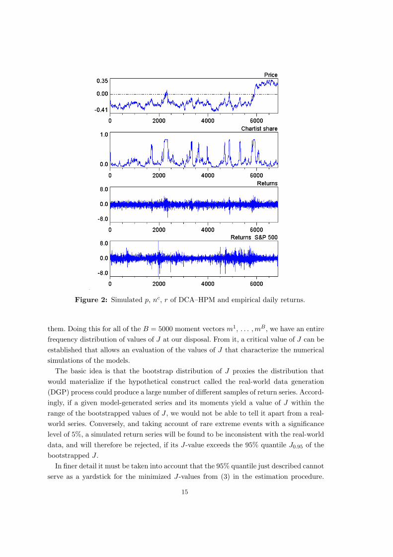
Figure 2 selects the herding variant of the discrete choice approach, i.e. DCA–HPM,to show the implications of the switching pattern for the evolution of prices and returns.First, there are some more chartist episodes than we observed for TPA–HPM, but on theother side the market fractions of this group are less conspicuous here. Second, despitethe overall dominance of fundamentalists, prices are persistently disconnected from thefundamental value. This is a remarkable phenomenon since it is not captured by thechoice of our moments and so did not enter the estimation. As a third point, the returnsdo seem to exhibit a certain clustering in volatility, although it does not come out so nicelyas in the empirical return series in the bottom panel. 12 Conforming to our intuition, theperiods of higher volatility are clearly seen to be caused by a temporary dominance ofchartists in the market. This interrelationship can be observed in all of the models andwe consider it a great theoretical merit of our approach to structural stochastic volatility.However, whether the model-generated clustering is satisfactorily close to the empiricalphenomenon is an issue for which the precise summary statistics need to be computedand compared.
4. Moment matching and model contest
4.1. Specification of a moment-specific p-value
After the straightforward MSM estimations have provided us with numerical values forthe structural parameters in each of our seven models, we are in the rest of the paperconcerned with a more detailed assessment of the quality of the moment matching thusachieved. The investigation begins with the most elementary question if some or all ofthe models would be rejected by the data. Although if taken literally this is a ratheracademic question since every stylized model, by definition, is ‘false’ anyway, it is a veryconvenient one that can be addressed from different angles.
Let us start out from the process of bootstrapping the empirical returns. While so farit served us to derive a variance-covariance matrix of the moments, the large sample ofmoments obtained by this procedure can also be used to apply the loss function J to
12 We could have also presented a more beautiful example in this respect.
14
Figure 2: Simulated p, nc, r of DCA–HPM and empirical daily returns.
them. Doing this for all of the B = 5000 moment vectors m1, . . . , mB, we have an entirefrequency distribution of values of J at our disposal. From it, a critical value of J can beestablished that allows an evaluation of the values of J that characterize the numericalsimulations of the models.
The basic idea is that the bootstrap distribution of J proxies the distribution thatwould materialize if the hypothetical construct called the real-world data generation(DGP) process could produce a large number of different samples of return series. Accord-ingly, if a given model-generated series and its moments yield a value of J within therange of the bootstrapped values of J , we would not be able to tell it apart from a real-world series. Conversely, and taking account of rare extreme events with a significancelevel of 5%, a simulated return series will be found to be inconsistent with the real-worlddata, and will therefore be rejected, if its J-value exceeds the 95% quantile J0.95 of thebootstrapped J .
In finer detail it must be taken into account that the 95% quantile just described cannotserve as a yardstick for the minimized J-values from (3) in the estimation procedure.
15
The reason is that, just in order to reduce the sample variability, these returns weresimulated over a time horizon S that was more than ten times as long as the samples ofthe returns from the bootstrap, where T ′ = 6750. Rather, for a meaningful comparisonto the bootstrapped J0.95, the J-values of model simulations of equal length T ′ must beutilized.
It goes without saying that the information from a single simulation run over therelatively short bootstrap period is not reliable enough for a final evaluation of a modelfit. Nevertheless, it is easy to undertake a Monte Carlo (MC) experiment and repeatthese simulations many times. In this way a distribution of model-generated J-values isobtained, which can subsequently be contrasted with the bootstrap distribution.
For a precise description of this method we emphasize that the bootstrapped momentsare extracted from the empirical returns by writing mb = mb({remp
t }T ′
t=1).13 Furthermore,
let θ be the estimated vector of a model’s structural parameters and indicate the differentrandom number sequences underlying the MC simulations by the letter c, giving rise tomoments m = mc(θ;T ′) (as in the bootstrap, we work with c = 1, . . . , 5000). Thefrequency distributions from the following two sets of J-values are then considered:
Bootstrap : { J [mb({rempt }T ′
t=1)] }5000
b=1
Monte Carlo : { J [mc(θ;T ′)] }5000
c=1
T ′ = 6750 (10)
Take model DCA–W as a first example. Here we obtain J0.95 = 22.45 as the critical valueof the bootstrapped loss function. As expected, the model-generated MC distribution ofJ is considerably wider to the right, such that J0.95 corresponds to its 22.7% quantile.For a succinct summary of the general moment matching it may therefore be said thatthe model has a p-value of 22.7%, with respect to the parameter vector θ from Table1, the data of the S&P 500 index, and the specific nine moments that we have chosen.This means that more than three-fourths of the simulations of the model over T ′ = 6750days would be rejected, while this is not possible for a bit more than one-fifth of them.Hence, according to the conventional significance criteria, the DCA–W model would notbe discarded as being obviously incompatible wit the empirical data. In fact, a p-valueof 22.7% does not seem to be a bad performance. 14
The moment-specific p-values of this and the other models are documented in Table 2,and the clear winner by far with a respectable value of more than 30 per cent is: DCA–HPM. Moreover, within both switching approaches DCA and TPA, the herding variant
13 It will be clear that these moments are those that have already been underlying the estimateof the variance-covariance matrix Σ in (5), which in turn yielded W as its inverse by eq. (4).14 In addition, there are good reasons to expect that the, so to speak, MC simulations of thereal-world DGP would yield a wider distribution of J than the bootstrap from the one realizationactually observed. In this respect, the p-value of 22.7% would be an underestimation ratherthan an overestimation. See Franke and Westerhoff (2010, Section 4) for an elaboration of thisargument.
16
DCA TPA
W WP WHP HPM W WP HPM
22.7 23.5 24.1 32.6 12.7 21.3 24.0
Table 2: Moment-specific p-values with respect to thebootstrap distribution of J of the empirical returns.
augmented by the predisposition and misalignment effects outperforms the variants withthe differential wealth effects. On the other hand, for each of the common specificationsof the attractiveness index, DCA outperforms TPA.
Nevertheless, if the present limitation to our nine moments as being sufficiently rep-resentative of the most relevant stylized facts of a major stock market index is accepted,and likewise the concept of the corresponding p-value as a criterion for not rejecting amodel, then all seven models have passed a first important test. We view this as someprogress over the merely qualitative assessments of a structural asset pricing model thatdeemed satisfactory only a couple of years ago.
4.2. Small-sample variability in pairwise model comparisons
The concept of the moment-specific and simulation-based p-value of a model averagesacross MC simulation runs with more realistic and less realistic outcomes, thus min-imizing the influence of sample variability. In this subsection we slightly change ourperspective and actually start out from the phenomenon of sample variability in a directcomparison of two models. Here we are aware that although one model may be superiorin terms of the p-value, it is nonetheless possible that its value of J from an arbitrar-ily selected simulation run is worse than that from an arbitrary simulation of the rivalmodel. We ask how often this can happen if the experiment is repeated many times. Inthis way we get another quantitative measure of how much better one model is thananother.
Specifically, we take the same 5000 MC simulations for each model over T ′ = 6750days that have been underlying Table 2. We now consider all of the possible pairings oftwo models M1 and M2, and for each pair the values J1(c), J2(c′) of the loss functionfrom the MC runs c, c′ = 1, . . . , 5000. Varying the influence of their sample variability,we make use of them in two different ways. First, we compare J1(c) to J2(c′) for all pairsc, c′ and count the number of cases where J1(c) < J2(c′). The first entry in each cell ofTable 3 reports them in per cent of all of these comparisons, which amount to a total of50002 = 25 millions.
Since the MSM estimations were based on simulations over a horizon that is ten times
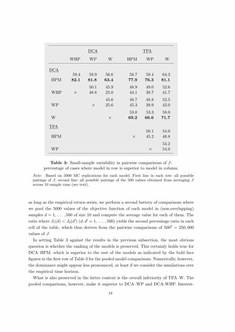
Table 3: Small-sample variability in pairwise comparisons of J :percentage of cases where model in row is superior to model in column.
Note: Based on 5000 MC replications for each model. First line in each row: all possiblepairings of J ; second line: all possible pairings of the 500 values obtained from averaging Jacross 10 sample runs (see text).
as long as the empirical return series, we perform a second battery of comparisons wherewe pool the 5000 values of the objective function of each model in (non-overlapping)samples d = 1, . . . , 500 of size 10 and compute the average value for each of them. Theratio where J1(d) < J2(d′) (d, d′ = 1, . . . , 500) yields the second percentage ratio in eachcell of the table, which thus derives from the pairwise comparisons of 5002 = 250, 000values of J .
In setting Table 3 against the results in the previous subsection, the most obviousquestion is whether the ranking of the models is preserved. This certainly holds true forDCA–HPM, which is superior to the rest of the models as indicated by the bold facefigures in the first row of Table 3 for the pooled model comparisons. Numerically, however,the dominance might appear less pronounced, at least if we consider the simulations overthe empirical time horizon.
What is also preserved in the latter context is the overall inferiority of TPA–W. Thepooled comparisons, however, make it superior to DCA–WP and DCA-WHP. Interest-
18
ingly, the significance of the pure wealth effects increases in greater generality. Integratingthem into DCA, which formerly yielded the third-worst position in Table 2, leads now toa better result; DCA–W gains second rank since it outperforms all models except DCA–HPM. In particular, it beats the more general versions DCA–WP and DCA–WHP, andthis superiority is remarkably strong for the pooled comparisons where DCA–W has alower value of J in roughly 75% of all cases (the complement of 25.0 and 25.6 in the thirdcolumn of Table 3.
It is similarly worth pointing out that TPA–WP improves from second-worst in Table2 to third-best in Table 3, while TPA–HPM deteriorates in relation to TPA–WP andTPA–W. These examples show that although being based on the same MC simulations,Table 2 and 3 process different information: Table 3 with the direct comparisons of twomodels and the values of the loss function, and Table 2 with the comparison of onesummarizing statistic of the frequency distributions of J . 15
The overall lesson that we take from these observations is that, even though Table2 can appear more meaningful because it limits the role of sample variability as faras possible, its more detailed quantitative results might not be overrated. This note ofcaution rather prompts us to consider an alternative criterion to evaluate the goodnessof the models’ moment matching.
4.3. Moment coverage ratios
The evaluation of the models in the previous subsections was based on the values of theobjective function J . While this allowed us to compare the models relative to each other,we could not tell how “well” they are able to match the moments. An immediate methodto address this question is to test the minimized value J of a model for the overidentifyingrestrictions, as there are more moments than parameters. If it is less than a certain criticalvalue derived from the χ2-distribution, the model would be considered to be valid withrespect to the selected moments. On the other hand, it is well-known that the conversecase is not necessarily an indication that the model fails to mimic the empirical data inseveral dimensions. 16
In this paper we use a more direct way to assess the degree of moment matchingof a model, which can also take each single moment into account. All we need is theconcept of a confidence interval of the empirical moments. Although it would be easiestto adopt the diagonal entries of the bootstrapped covariance matrix (5) for this purpose,we choose an alternative approach in case one feels uneasy about the bootstrapping
15 Nevertheless, the deterioration in the ranking of DCA–WP and DCA–WHP might lead oneto repeat their estimation with different random number seeds. We abstain from this extensionof the analysis for reasons of space and since DCA–HPM is so dominant over the other DCAversions.16 See Davidson and MacKinnon (2004, p. 368) for a short summarizing statement in this respect.Two elaborate studies on the subject are Kocherlakota (1990) and Mao (1990).
19
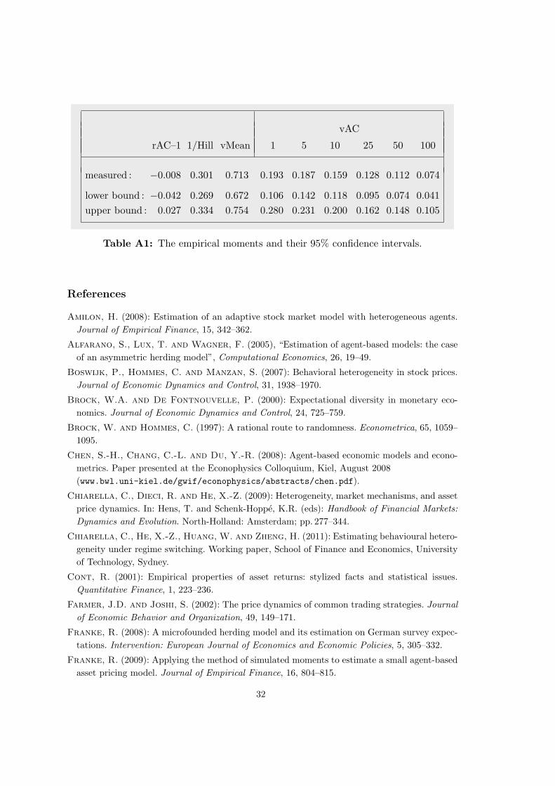
of the ACF at the longer lags. Except for the Hill moment, for which a theoreticalformula is available, the standard errors of the moments are obtained by conceiving theautocorrelation coefficients as (nonlinear) functions of the means, or time averages, ofsimpler expressions of the returns and applying the delta method to them (the details ofthese computations are given in the Appendix). On this basis, the 95% confidence intervalof a moment is defined as the interval with boundaries ±1.96 times the standard erroraround the empirical estimate. In addition, the slight smoothing of the single coefficientsin Section 2 with the centred three-lag averages is taken over (the lower and upper boundsof the confidence intervals are reported in Table A1 in the Appendix).
In this way we have a simple and intuitive criterion for a qualitative assessment ofa given return series that was simulated over the empirical time horizon: it cannot berejected as being incompatible with the data if all of its moments are contained in theconfidence intervals. Nevertheless, because of the sample variability a single series isclearly not sufficient to evaluate a model as a whole.
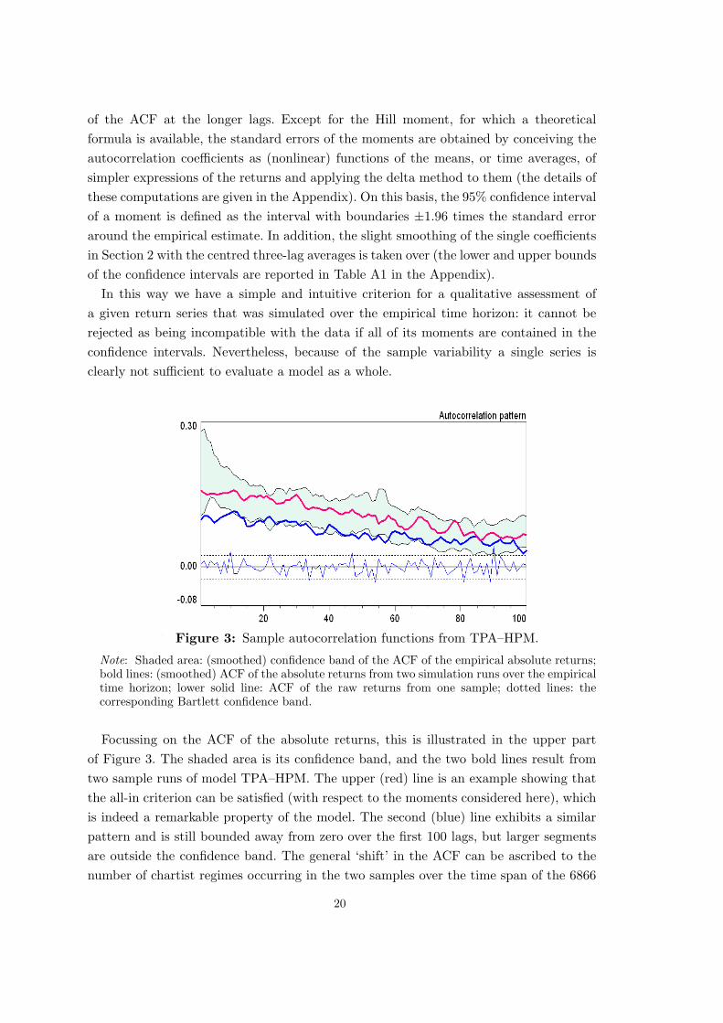
Figure 3: Sample autocorrelation functions from TPA–HPM.
Note: Shaded area: (smoothed) confidence band of the ACF of the empirical absolute returns;bold lines: (smoothed) ACF of the absolute returns from two simulation runs over the empiricaltime horizon; lower solid line: ACF of the raw returns from one sample; dotted lines: thecorresponding Bartlett confidence band.
Focussing on the ACF of the absolute returns, this is illustrated in the upper partof Figure 3. The shaded area is its confidence band, and the two bold lines result fromtwo sample runs of model TPA–HPM. The upper (red) line is an example showing thatthe all-in criterion can be satisfied (with respect to the moments considered here), whichis indeed a remarkable property of the model. The second (blue) line exhibits a similarpattern and is still bounded away from zero over the first 100 lags, but larger segmentsare outside the confidence band. The general ‘shift’ in the ACF can be ascribed to thenumber of chartist regimes occurring in the two samples over the time span of the 6866
20
days. The simulation producing the upper line gives rise to seven episodes where thechartists form a fair majority, while the lower bold line originates from a simulation runwith only four chartist regimes. Besides, the lower thin line in Figure 3, which displaysthe ACF of the raw returns of one of the simulation runs, is perfectly representativeand exemplifies once more that this—and the other models as well—have no difficulty inkeeping it insignificant.
It is now obvious to think of many simulation runs of a model for each of whichthe confidence interval check is repeated. This leads us to the concept of a coverageratio. That is, we count the number of Monte Carlo simulation runs for which the singlemoments, or all nine moments jointly, are contained in their confidence intervals anddefine the corresponding percentage numbers as the model’s moment coverage ratios.More briefly, they may also be denoted by the acronym MCR.
As the concept has been introduced, the central coverage ratio is certainly the jointMCR. Its values for the seven models are presented in the first row of Table 4. It willperhaps be expected that comparatively low values of the objective function J go along,more or less, with comparatively high coverage ratios. The table, however, reveals that theminimized values of J and the corresponding joint MCRs convey different information,which even leads to a different ranking of the models. In particular, the formerly dominantmodel DCA–HPM now only ranks fourth, whereas TPA–HPM as the model that in Tables2 and 3 was second or worse, now shows the best performance—and this with a distancefrom the other models.
There is one model (TPA–W) that misses the obvious benchmark value of 5%, andDCA–W (which formerly was among the best) is just at the margin. This is quite incontrast to their p-values with respect to the empirical bootstrap distribution of J inTable 2, which were distinctly higher than 5%. The other five models are not in opencontradiction to the data, neither on the basis of J nor on the basis of the joint MCRcriterion.
Beyond this qualitative statement, we would like to put the figures of the joint coverageratios in Table 4 into a quantitative perspective. To this end, consider the events thatthe sample moments from the true DGP process happen to fall into their confidenceintervals. If it were assumed that these events are all independent of each other, thetrue DGP would have a joint MCR of 0.959 = 63.0%. If more conservatively the factof a certain dependence among the events is approximated by the assumption that onlyfive of them are independent—say: r AC–1, Hill, v Mean, v AC–1 and v AC–100—then ajoint MCR of 77.4% would be obtained. Using the latter as a conservative benchmark towhich the fitting ratios from the Monte Carlo experiments may be related, the 10.1% ofthe DCA model with herding, predisposition and misalignment (HPM) corresponds toan effective MCR of 10.1/77.4 = 13.0%, and the 22.1% of the analogous TPA model toan effective MCR of 28.6%.
Another problem is that all of these statements are based on asymptotic theory. The
confidence intervals of the moments that we thereby obtained may or may not be a goodapproximation to the ones appropriate for small samples of the real-world DGP. Above,to get more information about the small sample properties, we applied the bootstrap tothe empirical returns. We can once more make use of the 5000 bootstrap samples forour present purpose, that is, we compute the joint MCR for them and employ it as ayardstick against which we can measure the MCRs of our models. The result, as shown inthe first column of the numbers in Table 4, is a ratio of 32.6%, which is considerably lowerthan the hypothetical reference figures of 77.4% or 63.0% that have just been mentioned.On the other hand, as it should be, the ratio of 32.6% is still distinctly higher than theMCRs of the models, though it does not degrade the latter completely.
The most obvious way to relate the models’ joint MCRs to that of the bootstrap isto express them as a fraction of it (in %). This is done in the second row of Table 4.Referring to these statistics, we only would reject TPA–W; already the figure of 15.5% forDCA–W as the second-worst model appears fairly acceptable, even though the remainingfive models perform much better. The best model, TPA–HPM, now reaches a level ofeven 67.9%. Nonetheless, this figure is probably an overestimation of a more appropriaterelative coverage statistic and should not be taken too literally. In any case, whatevermeasure we refer to, the degree of the model’s ability to match the moments we have
22
chosen is highly remarkable.Returning to the model ranking, TPA–HPM clearly outperforms DCA–HPM, which
was formerly so dominating. To see what mainly causes the reversal in the ranking, weshould have a look at the coverage ratios of the single moments in the lower part of Table4 and compare them across the models. It is thus found that there are only two momentsin which DCA–HPM is inferior to TPA–HPM, namely the Hill moment and the meanof the absolute returns. In all other moments, DCA–HPM has an edge over TPA–HPM,especially at the longer lags in ACF(v). Its lower joint MCR results from the fact thatthe superiority in the latter is less pronounced than the inferiority in v Mean and, mostdramatically, in the Hill moment.
The overall impression from the detailed model comparisons is the omnipresence oftrade-off effects. No model is, so to speak, Pareto inferior or superior to another model(except perhaps the WP and WHP versions of DCA, if we neglect the first momentwhich is almost perfectly matched by all models). In particular, the second-worst modelDCA–W has the highest MCRs of all models at the longer lags of ACF(v). Unfortunately,this positive result is wrecked by the bad match of v Mean and Hill. The more generalDCA–WHP is clearly better in this respect (even the best of all models), but at the priceof a serious deterioration of the last three moments. There are similar, though moremoderate examples for other pairwise model comparisons. On the whole, it turns outthat TPA–HPM has found the best compromise in the trade-offs.
4.4. The joint coverage ratio as an alternative estimation criterion
Table 4 has disproved the expectation that minimal values of the objective functionJ also imply a near-optimal ratio of a model’s joint moment matching. In particular,the formerly best model DCA–HPM only ranks fourth when evaluated in terms of thejoint MCR. Hence the question arises if a different choice of its structural parameterscould enhance its position; or, with respect to the presently best model TPA–HPM, ifwe could still improve its joint MCR of 22.1%. Most obviously, we are thus asking for themaximization of the joint MCR as an alternative estimation criterion. Unfortunately, adirect maximization would incur an extremely high computational cost. In addition, themany trade-offs that we have seen are likely to cause a larger (or even infinite) numberof local maxima of the joint coverage ratio.
To reduce the computational burden we resort to a heuristic procedure. Our idea isto modify the original loss function J and set up a version of which we hope that it isbetter suited for achieving high coverage ratios. To begin with, we disregard the cross-dependencies between the single moments in the weighting matrix. Since our goal is tohave the moments contained in their confidence intervals, the width of which are givenby roughly two times the standard error (SEi) of the moments i, we think of a diagonalweighting matrix with weights wii = 1/(SEi)2.
23
With such an objective function, a deviation of the simulated from the empiricalmoment i by one or two SEi, respectively, would yield a contribution of this moment tothe total value of the function of 1 or 4, respectively. However, in our explorations of thisidea we found out that penalizing the deviations in a quadratic way is not sufficientlystrong.
As a more flexible approach, the following specification proved useful then. Startingfrom the observation that the expressions di := | mi(θ;T, s) − memp
i | / SEi should fallshort of 1.96 if possible (s being an index to represent the random seed in the simulationof the model), we expect better chances if values of di close to or above this thresholdare disproportionately penalized. The simplest way to do so is to apply a piecewiselinear transformation function to di, where the change in the slope is described by twoparameters di and κi. The slope for values of di between zero and some critical valuedi somewhat below 1.96 is thus relatively flat compared to the slope when di > di.Without loss of generality, the slope over the first segment can be unity, and it is κi � 1when di > di. After some trial and error, we uniformly put di = d = 1.90, so that ourtransformation function reads,
F (di;κi) =
di if 0 ≤ di ≤ d
d + κi(di−d) if di ≥ d
d = 1.90 (11)
Given the moment-specific slopes κi, and given the index s of the random seed of asimulation run over the empirical time horizon T (s = 1, 2, . . . ), the total loss to whicha parameter set θ gives rise is the sum of the losses of the single moments in (11),
`(θ;T, s) :=9∑
i=1
F [ |mi(θ;T, s)−mempi |/ SEi ; κi ] (12)
To reduce the sample variability, these losses are finally averaged over a larger numberS of simulations. Dropping the explicit reference to T , this yields the loss function L =L(θ;S) with which we will work in the following:
L(θ;S) :=1S
S∑s=1
`(θ;T, s) (13)
We first applied the function to model TPA–HPM and explored whether it would thusbe possible to raise its joint MCR noticeably above the maximal 22.1% from Table 4.We began with S = 10 and later sharpened it to S = 100. Playing around with differentcombinations of the slope parameters κi, the trade-off effects were also (not surprisingly)found for the individual model. That is, an increase in the coverage ratios of one ortwo moments goes at the expense of some other moments. Generally, of course, theimplications for the joint coverage ratio are ambiguous. It nevertheless proved promisingto try to improve on the coverage ratio of the Hill estimator. Although this tends to
24
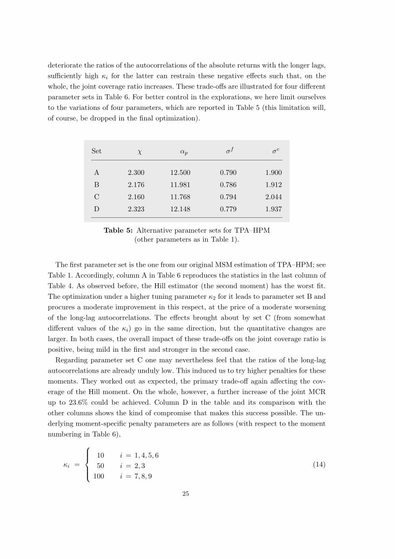
deteriorate the ratios of the autocorrelations of the absolute returns with the longer lags,sufficiently high κi for the latter can restrain these negative effects such that, on thewhole, the joint coverage ratio increases. These trade-offs are illustrated for four differentparameter sets in Table 6. For better control in the explorations, we here limit ourselvesto the variations of four parameters, which are reported in Table 5 (this limitation will,of course, be dropped in the final optimization).
Set χ αp σf σc
A 2.300 12.500 0.790 1.900
B 2.176 11.981 0.786 1.912
C 2.160 11.768 0.794 2.044
D 2.323 12.148 0.779 1.937
Table 5: Alternative parameter sets for TPA–HPM(other parameters as in Table 1).
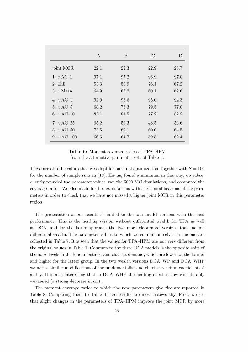
The first parameter set is the one from our original MSM estimation of TPA–HPM; seeTable 1. Accordingly, column A in Table 6 reproduces the statistics in the last column ofTable 4. As observed before, the Hill estimator (the second moment) has the worst fit.The optimization under a higher tuning parameter κ2 for it leads to parameter set B andprocures a moderate improvement in this respect, at the price of a moderate worseningof the long-lag autocorrelations. The effects brought about by set C (from somewhatdifferent values of the κi) go in the same direction, but the quantitative changes arelarger. In both cases, the overall impact of these trade-offs on the joint coverage ratio ispositive, being mild in the first and stronger in the second case.
Regarding parameter set C one may nevertheless feel that the ratios of the long-lagautocorrelations are already unduly low. This induced us to try higher penalties for thesemoments. They worked out as expected, the primary trade-off again affecting the cov-erage of the Hill moment. On the whole, however, a further increase of the joint MCRup to 23.6% could be achieved. Column D in the table and its comparison with theother columns shows the kind of compromise that makes this success possible. The un-derlying moment-specific penalty parameters are as follows (with respect to the momentnumbering in Table 6),
κi =
10 i = 1, 4, 5, 650 i = 2, 3
100 i = 7, 8, 9
(14)
25
A B C D
joint MCR 22.1 22.3 22.9 23.7
1: r AC–1 97.1 97.2 96.9 97.0
2: Hill 53.3 58.9 76.1 67.2
3: v Mean 64.9 63.2 60.1 62.6
4: v AC–1 92.0 93.6 95.0 94.3
5: v AC–5 68.2 73.3 79.5 77.0
6: v AC–10 83.1 84.5 77.2 82.2
7: v AC–25 65.2 59.3 48.5 53.6
8: v AC–50 73.5 69.1 60.0 64.5
9: v AC–100 66.5 64.7 59.5 62.4
Table 6: Moment coverage ratios of TPA–HPMfrom the alternative parameter sets of Table 5.
These are also the values that we adopt for our final optimization, together with S = 100for the number of sample runs in (13). Having found a minimum in this way, we subse-quently rounded the parameter values, ran the 5000 MC simulations, and computed thecoverage ratios. We also made further explorations with slight modifications of the para-meters in order to check that we have not missed a higher joint MCR in this parameterregion.
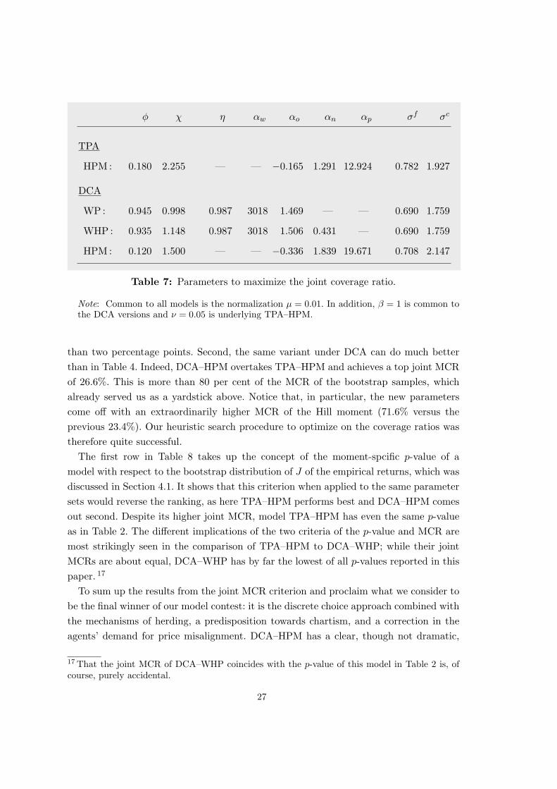
The presentation of our results is limited to the four model versions with the bestperformance. This is the herding version without differential wealth for TPA as wellas DCA, and for the latter approach the two more elaborated versions that includedifferential wealth. The parameter values to which we commit ourselves in the end arecollected in Table 7. It is seen that the values for TPA–HPM are not very different fromthe original values in Table 1. Common to the three DCA models is the opposite shift ofthe noise levels in the fundamentalist and chartist demand, which are lower for the formerand higher for the latter group. In the two wealth versions DCA–WP and DCA–WHPwe notice similar modifications of the fundamentalist and chartist reaction coefficients φ
and χ. It is also interesting that in DCA–WHP the herding effect is now considerablyweakened (a strong decrease in αn).
The moment coverage ratios to which the new parameters give rise are reported inTable 8. Comparing them to Table 4, two results are most noteworthy. First, we seethat slight changes in the parameters of TPA–HPM improve the joint MCR by more
Table 7: Parameters to maximize the joint coverage ratio.
Note: Common to all models is the normalization µ = 0.01. In addition, β = 1 is common tothe DCA versions and ν = 0.05 is underlying TPA–HPM.
than two percentage points. Second, the same variant under DCA can do much betterthan in Table 4. Indeed, DCA–HPM overtakes TPA–HPM and achieves a top joint MCRof 26.6%. This is more than 80 per cent of the MCR of the bootstrap samples, whichalready served us as a yardstick above. Notice that, in particular, the new parameterscome off with an extraordinarily higher MCR of the Hill moment (71.6% versus theprevious 23.4%). Our heuristic search procedure to optimize on the coverage ratios wastherefore quite successful.
The first row in Table 8 takes up the concept of the moment-spcific p-value of amodel with respect to the bootstrap distribution of J of the empirical returns, which wasdiscussed in Section 4.1. It shows that this criterion when applied to the same parametersets would reverse the ranking, as here TPA–HPM performs best and DCA–HPM comesout second. Despite its higher joint MCR, model TPA–HPM has even the same p-valueas in Table 2. The different implications of the two criteria of the p-value and MCR aremost strikingly seen in the comparison of TPA–HPM to DCA–WHP; while their jointMCRs are about equal, DCA–WHP has by far the lowest of all p-values reported in thispaper. 17
To sum up the results from the joint MCR criterion and proclaim what we consider tobe the final winner of our model contest: it is the discrete choice approach combined withthe mechanisms of herding, a predisposition towards chartism, and a correction in theagents’ demand for price misalignment. DCA–HPM has a clear, though not dramatic,
17 That the joint MCR of DCA–WHP coincides with the p-value of this model in Table 2 is, ofcourse, purely accidental.
27
TPA–HPM DCA–WP DCA–WHP DCA–HPM
‘p-value’ 24.0 10.2 8.7 19.5
joint MCR 24.4 23.8 24.1 26.6
in % of 32.6 74.8 73.0 73.9 81.6
1: r AC–1 97.0 97.4 96.9 97.5
2: Hill 62.9 86,4 86,7 71.6
3: v Mean 64.7 66.8 65.9 55.8
4: v AC–1 94.7 100.0 100.0 99.5
5: v AC–5 75.9 95.8 96.4 93.5
6: v AC–10 84.6 89.8 88.5 90.0
7: v AC–25 59.0 79.8 79.7 79.4
8: v AC–50 70.2 67.8 69.7 84.4
9: v AC–100 65.2 49.5 51.1 70.5
Table 8: Moment coverage ratios (in %)obtained from minimizing the loss function (11) – (13).
Note: The figures in the first row are the moment-specific p-values with respect to the bootstrapdistribution of J of the empirical returns, described in Section 4.1. The figure of 32.6% in thethird row is the joint MCR of the bootstrap samples (see Table 4).
edge over the same mechanisms within the framework of the transition probability ap-proach, and over the DCA versions that incorporate the effects of differential wealth.The performance of the last three models is about equal. More generally, the momentcoverage ratios in Table 8 provide a remarkable benchmark against which we would liketo measure other models of speculative asset price dynamics.
5. Conclusion
In recent years, agent-based asset pricing models have made remarkable progress in repli-cating a diverse set of central statistical features of financial market time series. In thisendeavour, the present paper has focussed on a new class of models which is based onthe concept of structural stochastic volatility. This framework lets the market partici-pants choose between a noisy technical and a noisy fundamental trading strategy, wheregenerally the choice is governed by four socio-economic principles. In short, they includedifferential wealth, herding, a behavioral predisposition towards one of the strategies,
28
and a misalignment correction mechanism, i.e. a propensity to withdraw from chartismas the gap between prices and the fundamental value widens. A switching index intowhich a combination of these components is aggregated is then the driving variable in,alternatively, the discrete choice approach or the transition probability approach, whichare two convenient devices from the literature to determine the market shares of the twogroups of traders. Simulations show that the resulting variations in the overall noise leveland in the stabilizing and destabilizing tendencies of the strategies can lead to irregularswitches between rather volatile and rather calm market regimes. More specifically, phe-nomena such as volatility clustering, long memory effects and fat tails may thus comeabout.
Having thus a promising collection of different models at hand, we put them to moreformal tests. To this end we estimated them with two variants of the method of simulatedmoments, both of which seek to bring certain model-implied summary statistics (the‘moments’), which correspond to the stylized facts of interest, as close as possible totheir empirical counterparts. In the first case, ‘closeness’ is represented by the distancebetween these moments as it is measured by a quadratic loss function. For the second casewe introduced the concept of a (joint) moment coverage ratio (MCR). Here the modelsare repeatedly simulated over the empirical time horizon and we count the number oftimes where all of the simulated moments are contained in the empirical confidenceintervals. MCR is therefore another, apparently new way of summarizing how often thedata from a model and the real market could not be told apart.
Accepting our (or a similar) choice of moments, both approaches provide us with atransparent and not too technical criterion to assess the overall fit of a model. This isindeed something that the burgeoning field of agent-based financial market models iscurrently in need of. So many models have been put forward that we are now facing the“wilderness of bounded rationality problem” (Hommes, 2011, p. 2), meaning that thereare too many degrees of freedom to set up good models. At this stage some guidance isrequired to judge which models can mimic the stylized facts, say, “fairly well” and whichare even “very good” in this way. A basic methodological message of our paper is thatthe method of simulated moments, with the specifications here proposed, is a superb toolto serve this purpose.
Actually, the present study suggests a general call for model contest—and its resultsare a good point of departure for that. On the one hand, we have identified mechanismsthat are already quite efficient in matching the desired moments, the clear winner ofthe model contest in this paper being DCA–HPM: the discrete choice approach thatincorporates herding with a certain predisposition towards chartism, which is howevertamed by the misalignment correction mechanism.
On the other hand, concerning the quantitative performance of this model, it maybe recalled that we bootstrapped a (moment-specific) p-value of 32.6% for it, and thataccording to the MCR criterion no less than 26.6 per cent of the simulations are indis-
29
tinguishable from the empirical data. Our view is that these statistics set a standard formodel validation and model selection, and raising these benchmarks may be acceptedas a challenge to existing models and to future model building. This is not to say thatgoodness-of-fit along these or similar lines is the only criterion to evaluate competingmodels. In future research it should, however, be worked out clearly what other featuresmight compensate for a possible inferiority in this respect.
Appendix: Standard errors of the empirical moments
Let us begin with the Hill moment, which we base on a conventional tail size of five percent. Arranging the absolute returns in descending order, v(1) ≥ v(2) ≥ . . . ≥ v(T ), andputting k = 0.05 · T (rounded to an integer number), the Hill estimator is equal to thereciprocal of
γ := (1/k)k∑
i=1
ln v(i) − ln v(k)
The fact that this estimator is necessarily biased need not concern us here since it appliesto the empirical and model-generated data alike. Its asymptotic normality has been shownby, e.g., Goldie and Smith (1987) or Hall (1990), for which they obtain the variance
Var(γ) = γ2 / k
Certainly, in applications the ‘true’ value γ is replaced with the estimate γ. The momentcoverage ratios relate to γ rather than the Hill estimator 1/γ itself.
The computation of the standard errors of the other moments makes use of the deltamethod. We first give the general argument and then apply it for our special purpose. Tothis end, we refer to {zt}T
t=1 as a time series of a state vector zt of arbitrary dimension,zt ∈ IRn. In particular, to deal with the autocovariances the components of zt maybe vt, vt−1, etc. Let there be k ‘raw’ moments, a suitable combination of which yieldour (composed) moments of the autocovariances or autocorrelations. Furthermore, letf : IRn → IRk be a continuous function, and µ ∈ IRk the corresponding vector of theestimated (unconditional) raw moments,
µ =1T
T∑t=1
f(zt) (A15)
Since (A15) is a consistent and asymptotically normal estimator of µ = E[f(xt)], wehave with respect to its covariance matrix Σ ∈ IRk×k and the true raw moments µo,
√T (µ− µo) a∼ N(0,Σ)
An HAC estimator of Σ is the following Newey-West matrix for some suitable lag lengthp,
30
Σ = Γ(0) +p∑
h=1
(1− h
p + 1) [ Γ(h) + Γ(h)′ ]
Γ(h) =1T
T∑t=h+1
[f(zt)− µ] [f(zt−h)− µ]′ , h = 0, 1, . . . , p
We follow a usual practice and set p equal to the smallest integer greater than or equalto T 1/4 (Greene, 2002, p. 267, fn10).
Next, let θ ∈ IR be a summary statistic of zt which is determined by the raw momentsµ via a continuously differentiable and monotonic real function g : IRk → IR. That is, θ
is estimated as
θ = g(µ)
Putting θo = g(µo) and employing the delta method (cf. Davidson and MacKinnon, 2004,pp. 207f), we know that
√T (θ − θo) a∼ N(0, σ2)
and that the asymptotic variance σ2 can be estimated as
σ2 =∂g(µ)∂µ′
Σ∂g(µ)∂µ
(A16)
To obtain the standard error of the estimates of θ, it remains to divide σ by√
T .We can then turn to the application of (A16) to the correlation coefficient ρ between
The specification of the corresponding functions fi = fi(xt, yt), i = 1, . . . , 5, is obvious(f1(xt, yt) = xt, etc.) and with σx =
√µxx − µ2
x2y, σy =
√µyy − µ2
y , the vector of thepartial derivatives of g is computed as
∂g
∂µ′=
(ρ µx
σ2x
− µy
σxσy,
ρ µy
σ2y
− µx
σxσy,−ρ
2σ2x
,−ρ
2σ2y
,1
σxσy
)The lower and upper boundaries of the confidence intervals around the empirical sum-mary statistics that we thus obtain are documented in Table A1 (the autocorrelations ofthe absolute returns being smoothed as described in footnote 5).
Table A1: The empirical moments and their 95% confidence intervals.
References
Amilon, H. (2008): Estimation of an adaptive stock market model with heterogeneous agents.Journal of Empirical Finance, 15, 342–362.
Alfarano, S., Lux, T. and Wagner, F. (2005), “Estimation of agent-based models: the caseof an asymmetric herding model”, Computational Economics, 26, 19–49.
Boswijk, P., Hommes, C. and Manzan, S. (2007): Behavioral heterogeneity in stock prices.Journal of Economic Dynamics and Control, 31, 1938–1970.
Brock, W.A. and De Fontnouvelle, P. (2000): Expectational diversity in monetary eco-nomics. Journal of Economic Dynamics and Control, 24, 725–759.
Brock, W. and Hommes, C. (1997): A rational route to randomness. Econometrica, 65, 1059–1095.
Chen, S.-H., Chang, C.-L. and Du, Y.-R. (2008): Agent-based economic models and econo-metrics. Paper presented at the Econophysics Colloquium, Kiel, August 2008(www.bwl.uni-kiel.de/gwif/econophysics/abstracts/chen.pdf).
Chiarella, C., Dieci, R. and He, X.-Z. (2009): Heterogeneity, market mechanisms, and assetprice dynamics. In: Hens, T. and Schenk-Hoppe, K.R. (eds): Handbook of Financial Markets:Dynamics and Evolution. North-Holland: Amsterdam; pp. 277–344.
Chiarella, C., He, X.-Z., Huang, W. and Zheng, H. (2011): Estimating behavioural hetero-geneity under regime switching. Working paper, School of Finance and Economics, Universityof Technology, Sydney.
Cont, R. (2001): Empirical properties of asset returns: stylized facts and statistical issues.Quantitative Finance, 1, 223–236.
Farmer, J.D. and Joshi, S. (2002): The price dynamics of common trading strategies. Journalof Economic Behavior and Organization, 49, 149–171.
Franke, R. (2008): A microfounded herding model and its estimation on German survey expec-tations. Intervention: European Journal of Economics and Economic Policies, 5, 305–332.
Franke, R. (2009): Applying the method of simulated moments to estimate a small agent-basedasset pricing model. Journal of Empirical Finance, 16, 804–815.
32
Franke, R. and Westerhoff, F. (2009): Validation of a structural stochastic volatility modelof asset pricing. Working Paper, Universities of Kiel and Bamberg.(www.bwl.uni-kiel.de/gwif/downloads_papers.php?lang=en).
Franke, R. and Westerhoff, F. (2011): Estimation of a structural stochastic volatility modelof asset pricing. Computational Economics (in press).
Gilli, M. and Winker, P. (2003): A global optimization heuristic for estimating agent basedmodels. Computational Statistics and Data Analysis, 42, 299–312.
Goldie, C.M. and Smith, R.L. (1987): Slow variation with remainder: Theory and applica-tions. Quarterly Journal of Mathematics, Oxford 2nd Series, 38, 45–71.
Hall, P. (1990): Using the bootstrap to estimate mean square error and select smoothing para-meters in non-parametric problems. Journal of Multivariate Analysis, 32, 177–203.
Hevia, C. (2008): Standard errors using the delta method and GMM. mimeo.
Hommes, C. (2006): Heterogeneous agent models in economics and finance. In: Tesfatsion, L.and Judd, K. (eds): Handbook of Computational Economics, Vol. 2: Agent-Based ComputationalEconomics. North-Holland: Amsterdam; pp. 1107–1186.
Hommes, C. (2011): The heterogeneous expectations hypothesis: Some evidence from the lab.Journal of Economic Dynamics and Control, 35, 1–24.
Kocherlakota, N.R. (1990): On tests of representative consumer asset pricing models. Journalof Monetary Economics, 26, 285–304.
LeBaron, B. (2006): Agent-based computational finance. In: Tesfatsion, L. and Judd, K. (eds):Handbook of Computational Economics, Vol. 2: Agent-Based Computational Economics. North-Holland: Amsterdam; pp. 1187–1233.
Lee, B.-S. and Ingram, B.F. (1991): Simulation estimation of time series models. Journal ofEconometrics, 47, 197–205.
Li,Y., Donkers, B. and Melenberg, B. (2010): Econometric analysis of microscopic simula-tion models. Quantitative Finance, 10, 1187–1201.
Lux, T. (1995): Herd behaviour, bubbles and crashes. Economic Journal, 105, 881–889.
Lux, T. (2009): Stochastic behavioural asset-pricing models and the stylized facts. In: Hens,T. and Schenk-Hoppe, K.R. (eds.): Handbook of Financial Markets: Dynamics and Evolution.North-Holland: Amsterdam; pp. 161–216.
Lux, T. and Ausloos, M. (2002): Market fluctuations I: Scaling, multiscaling, and their possibleorigins. In: Bunde, A., Kropp, J. and Schellnhuber, H. (eds): Science of Disaster: ClimateDisruptions, Heart Attacks, and Market Crashes. Springer: Berlin; pp. 373–410.
Manzan, S. and Westerhoff, F. (2007), “Heterogeneous expectations, exchange rate dynam-ics and predictability”, Journal of Economic Behavior and Organization, 64, 111–128.
Mao, C.S. (1990): Hypothesis testing and finite sample properties of generalized method ofmoments estimators: A Monte Carlo study. Federal Reserve Bank of Richmond, Working Paper90–12.
Press, W.H. et al. (1986), Numerical Recipes: The Art of Scientific Computing. CambridgeUniversity Press: Cambridge, UK.
Weidlich, W. and Haag, G. (1983): Concepts and Models of a Quantitative Sociology: The
33
Dynamics of Interacting Populations. Berlin: Springer.
Westerhoff, F. (2009): Exchange rate dynamics: A nonlinear survey. In: Rosser, J.B., Jr. (ed.):Handbook of Research on Complexity. Edward Elgar: Cheltenham; pp. 287–325.
Winker, P., Gilli, M. and Jeleskovic, V. (2007): An objective function for simulationbased inference on exchange rate data. Journal of Economic Interaction and Coordination, 2,125–145.
34
BERG Working Paper Series on Government and Growth
1 Mikko Puhakka and Jennifer P. Wissink, Multiple Equilibria and Coordination Failure in Cournot Competition, December 1993
2 Matthias Wrede, Steuerhinterziehung und endogenes Wachstum, December 1993
3 Mikko Puhakka, Borrowing Constraints and the Limits of Fiscal Policies, May 1994
4 Gerhard Illing, Indexierung der Staatsschuld und die Glaubwürdigkeit der Zentralbank in einer Währungsunion, June 1994
5 Bernd Hayo, Testing Wagner`s Law for Germany from 1960 to 1993, July 1994
6 Peter Meister and Heinz-Dieter Wenzel, Budgetfinanzierung in einem föderalen System, October 1994
7 Bernd Hayo and Matthias Wrede, Fiscal Policy in a Keynesian Model of a Closed Mon-etary Union, October 1994
8 Michael Betten, Heinz-Dieter Wenzel, and Matthias Wrede, Why Income Taxation Need Not Harm Growth, October 1994
9 Heinz-Dieter Wenzel (Editor), Problems and Perspectives of the Transformation Process in Eastern Europe, August 1995
10 Gerhard Illing, Arbeitslosigkeit aus Sicht der neuen Keynesianischen Makroökonomie, September 1995
11 Matthias Wrede, Vertical and horizontal tax competition: Will uncoordinated Leviathans end up on the wrong side of the Laffer curve? December 1995
12 Heinz-Dieter Wenzel and Bernd Hayo, Are the fiscal Flows of the European Union Budget explainable by Distributional Criteria? June 1996
13 Natascha Kuhn, Finanzausgleich in Estland: Analyse der bestehenden Struktur und Überlegungen für eine Reform, June 1996
14 Heinz-Dieter Wenzel, Wirtschaftliche Entwicklungsperspektiven Turkmenistans, July 1996
15 Matthias Wrede, Öffentliche Verschuldung in einem föderalen Staat; Stabilität, vertikale Zuweisungen und Verschuldungsgrenzen, August 1996
16 Matthias Wrede, Shared Tax Sources and Public Expenditures, December 1996
17 Heinz-Dieter Wenzel and Bernd Hayo, Budget and Financial Planning in Germany, Feb-ruary 1997
18 Heinz-Dieter Wenzel, Turkmenistan: Die ökonomische Situation und Perspektiven wirt-schaftlicher Entwicklung, February 1997
19 Michael Nusser, Lohnstückkosten und internationale Wettbewerbsfähigkeit: Eine kriti-sche Würdigung, April 1997
20 Matthias Wrede, The Competition and Federalism - The Underprovision of Local Public Goods, September 1997
21 Matthias Wrede, Spillovers, Tax Competition, and Tax Earmarking, September 1997
22 Manfred Dauses, Arsène Verny, Jiri Zemánek, Allgemeine Methodik der Rechtsanglei-chung an das EU-Recht am Beispiel der Tschechischen Republik, September 1997
23 Niklas Oldiges, Lohnt sich der Blick über den Atlantik? Neue Perspektiven für die aktu-elle Reformdiskussion an deutschen Hochschulen, February 1998
24 Matthias Wrede, Global Environmental Problems and Actions Taken by Coalitions, May 1998
25 Alfred Maußner, Außengeld in berechenbaren Konjunkturmodellen – Modellstrukturen und numerische Eigenschaften, June 1998
26 Michael Nusser, The Implications of Innovations and Wage Structure Rigidity on Eco-nomic Growth and Unemployment: A Schumpetrian Approach to Endogenous Growth Theory, October 1998
27 Matthias Wrede, Pareto Efficiency of the Pay-as-you-go Pension System in a Three-Period-OLG Modell, December 1998
28 Michael Nusser, The Implications of Wage Structure Rigidity on Human Capital Accu-mulation, Economic Growth and Unemployment: A Schumpeterian Approach to Endog-enous Growth Theory, March 1999
29 Volker Treier, Unemployment in Reforming Countries: Causes, Fiscal Impacts and the Success of Transformation, July 1999
30 Matthias Wrede, A Note on Reliefs for Traveling Expenses to Work, July 1999
31 Andreas Billmeier, The Early Years of Inflation Targeting – Review and Outlook –, Au-gust 1999
32 Jana Kremer, Arbeitslosigkeit und Steuerpolitik, August 1999
33 Matthias Wrede, Mobility and Reliefs for Traveling Expenses to Work, September 1999
34 Heinz-Dieter Wenzel (Herausgeber), Aktuelle Fragen der Finanzwissenschaft, February 2000
35 Michael Betten, Household Size and Household Utility in Intertemporal Choice, April 2000
36 Volker Treier, Steuerwettbewerb in Mittel- und Osteuropa: Eine Einschätzung anhand der Messung effektiver Grenzsteuersätze, April 2001
37 Jörg Lackenbauer und Heinz-Dieter Wenzel, Zum Stand von Transformations- und EU-Beitrittsprozess in Mittel- und Osteuropa – eine komparative Analyse, May 2001
38 Bernd Hayo und Matthias Wrede, Fiscal Equalisation: Principles and an Application to the European Union, December 2001
39 Irena Dh. Bogdani, Public Expenditure Planning in Albania, August 2002
40 Tineke Haensgen, Das Kyoto Protokoll: Eine ökonomische Analyse unter besonderer Berücksichtigung der flexiblen Mechanismen, August 2002
41 Arben Malaj and Fatmir Mema, Strategic Privatisation, its Achievements and Challeng-es, Januar 2003
42 Borbála Szüle 2003, Inside financial conglomerates, Effects in the Hungarian pension fund market, January 2003
43 Heinz-Dieter Wenzel und Stefan Hopp (Herausgeber), Seminar Volume of the Second European Doctoral Seminar (EDS), February 2003
44 Nicolas Henrik Schwarze, Ein Modell für Finanzkrisen bei Moral Hazard und Überin-vestition, April 2003
45 Holger Kächelein, Fiscal Competition on the Local Level – May commuting be a source of fiscal crises?, April 2003
46 Sibylle Wagener, Fiskalischer Föderalismus – Theoretische Grundlagen und Studie Un-garns, August 2003
47 Stefan Hopp, J.-B. Say’s 1803 Treatise and the Coordination of Economic Activity, July 2004
48 Julia Bersch, AK-Modell mit Staatsverschuldung und fixer Defizitquote, July 2004
49 Elke Thiel, European Integration of Albania: Economic Aspects, November 2004
50 Heinz-Dieter Wenzel, Jörg Lackenbauer, and Klaus J. Brösamle, Public Debt and the Future of the EU's Stability and Growth Pact, December 2004
51 Holger Kächelein, Capital Tax Competition and Partial Cooperation: Welfare Enhancing or not? December 2004
52 Kurt A. Hafner, Agglomeration, Migration and Tax Competition, January 2005
53 Felix Stübben, Jörg Lackenbauer und Heinz-Dieter Wenzel, Eine Dekade wirtschaftli-cher Transformation in den Westbalkanstaaten: Ein Überblick, November 2005
54 Arben Malaj, Fatmir Mema and Sybi Hida, Albania, Financial Management in the Edu-cation System: Higher Education, December 2005
55 Osmat Azzam, Sotiraq Dhamo and Tonin Kola, Introducing National Health Accounts in Albania, December 2005
56 Michael Teig, Fiskalische Transparenz und ökonomische Entwicklung: Der Fall Bosni-en-Hercegovina, März 2006
57 Heinz-Dieter Wenzel (Herausgeber), Der Kaspische Raum: Ausgewählte Themen zu Politik und Wirtschaft, Juli 2007
58 Tonin Kola and Elida Liko, An Empirical Assessment of Alternative Exchange Rate Regimes in Medium Term in Albania, Januar 2008
59 Felix Stübben, Europäische Energieversorgung: Status quo und Perspektiven, Juni 2008 60 Holger Kächelein, Drini Imami and Endrit Lami, A new view into Political Business
Cycles: Household Expenditures in Albania, July 2008
61 Frank Westerhoff, A simple agent-based financial market model: direct interactions and comparisons of trading profits, January 2009
62 Roberto Dieci and Frank Westerhoff, A simple model of a speculative housing market, February 2009
63 Carsten Eckel, International Trade and Retailing, April 2009
64 Björn-Christopher Witte, Temporal information gaps and market efficiency: a dynamic behavioral analysis, April 2009
65 Patrícia Miklós-Somogyi and László Balogh, The relationship between public balance and inflation in Europe (1999-2007), June 2009
66 H.-Dieter Wenzel und Jürgen Jilke, Der Europäische Gerichtshof EuGH als Bremsklotz einer effizienten und koordinierten Unternehmensbesteuerung in Europa?, November 2009
67 György Jenei, A Post-accession Crisis? Political Developments and Public Sector Mod-ernization in Hungary, December 2009
68 Marji Lines and Frank Westerhoff, Effects of inflation expectations on macroeconomic dynamics: extrapolative versus regressive expectations, December 2009
69 Stevan Gaber, Economic Implications from Deficit Finance, January 2010
70 Abdulmenaf Bexheti, Anti-Crisis Measures in the Republic of Macedonia and their Ef-fects – Are they Sufficient?, March 2010
71 Holger Kächelein, Endrit Lami and Drini Imami, Elections Related Cycles in Publicly Supplied Goods in Albania, April 2010
72 Annamaria Pfeffer, Staatliche Zinssubvention und Auslandsverschuldung: Eine Mittel-wert-Varianz-Analyse am Beispiel Ungarn, April 2010
73 Arjan Tushaj, Market concentration in the banking sector: Evidence from Albania, April 2010
74 Pál Gervai, László Trautmann and Attila Wieszt, The mission and culture of the corpo-ration, October 2010
75 Simone Alfarano and Mishael Milaković, Identification of Interaction Effects in Survey Expectations: A Cautionary Note, October 2010
76 Johannes Kalusche, Die Auswirkungen der Steuer- und Sozialreformen der Jahre 1999-2005 auf die automatischen Stabilisatoren Deutschlands, October 2010
77 Drini Imami, Endrit Lami and Holger Kächelein, Political cycles in income from pri-vatization – The case of Albania, January 2011
78 Reiner Franke and Frank Westerhoff, Structural Stochastic Volatility in Asset Pricing Dynamics: Estimation and Model Contest, April 2011