STRUCTURAL STUDIES OF BLOCK COPOLYMER AND BLOCK COPOLYMER/ALUMINOSILICATE MATERIALS A Dissertation Presented to the Faculty of the Graduate School of Cornell University in Partial Fulfillment of the Requirements for the Degree of Doctor of Philosophy by Gilman Ewan Stephen Toombes August 2007
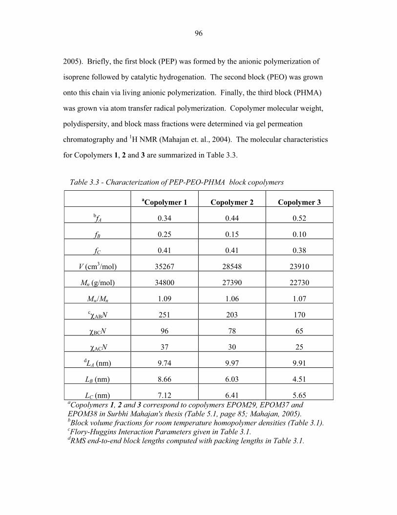
Transcript
STRUCTURAL STUDIES OF BLOCK COPOLYMER AND BLOCK
COPOLYMER/ALUMINOSILICATE MATERIALS
A Dissertation
Presented to the Faculty of the Graduate School
of Cornell University
in Partial Fulfillment of the Requirements for the Degree of
Jochen Gutmann, Dag Arneson, Dan Schuette, Nozomi Ando, Buz Barstow, Gideon
Alon, Joe Zinter, Jamie Chung, Peter Busch, Chae Un Kim, Lucas Koerner, Darol
Chamberlain, Hugh Philipp, Darren Southworth, Yi-fan Chen, Tom Caswell,
Elizabeth Landrum and Marianne Pouchet for their friendship and help. Special
thanks are due to Paul, Adam, Dan and Lucas for administering the lab's computer
system, Marty and Ann Marie Novak for inviting the entire lab to their house every
summer for the annual "Marty Party" extravaganza and Matt, Lisa Kwok and Thalia
Mills for the hikes, tightly-contested rounds of miniature golf and countless other
weekend adventures.
I wish to thank the many people in the physics department who have helped
me, including Greg Werner, Harald Pfeiffer, Karen Daniels, Jonathan Wrubel, Eileen
Tan, Andrew Perrella, Michael Berninger, Tom Glickman, Harsh Vishwasrao, Kat
Cicak, Richard Yeh, Bjoern Lange, Lauren Hsu, Anjali Gopalakrishnan, K Narayan,
vi
Nilay Pradhan, Abhay Pasupathy, Mandar Deshkmuth, Chris Deufel, Shaffique Adam,
Jeandrew Brink, Eric Ryan and Allie King, Luke Donev, Robin Smith, Curry Taylor,
Greg Stiesberg, Carl Franck, Monica Plisch, Don Holcomb, Persis Drell, Mike Teter,
Dan Ralph, Viet Elser, Rob Thorne, Eric Smith, Phil Krasicky, Vince Kotmel, Judy
Wilson, Rosemary French, Lisa Margosian and Deb Hatfield. Thank you also to thank
Nev Singhota, Kevin Dilley, Jane Earle, Juliane Bauer-Hutchinson and the other
members of the Cornell Center for Materials Research Outreach program.
While in Ithaca I have greatly appreciated the fellowship at Cornell Protestant
Cooperative Ministries lead by the Reverend Taryn Mattice and I am deeply indebted
to Taryn and many members of the PCM congregation including Ed Chan, Dan
Plafcan, Pauline Kusiak, Nathan Edwards, Amy Heusinkveld, David Baer, Robert
Mann-Thompson, Andrew North, Scott Bellen, Jill Wason, John Glauber, Clark
Smith, Julie Gosse, Sam Hess, Danny Fredrickson, Carolyn Stedinger, Nikki Kalbing,
Meg Richards and Chris Magnano.
I also must thank Dorothy, Dan and Henri Schuette and Taryn, Terry and Noah
Mattice for sharing the joy of seeing the world through young eyes.
Thank you to Leanne Duffy, Howard Wiseman, Sara Schneider, Kate Eltham,
Andrew and Angela Rae and my brother Spencer, and his wife, Kay, for visiting
Ithaca, my brother, Luke, for traveling around Utah, Rod Jory for hosting visits to
Canada and England and Thalia for visiting my family in Australia.
Finally, I thank my parents, Ewan and Judith, and my siblings Spencer, Luke
and Ngaio for their continual love and support.
vii
TABLE OF CONTENTS
BIOGRAPHICAL SKETCH ........................................................................ iii ACKNOWLEDGMENTS ............................................................................ iv TABLE OF CONTENTS ............................................................................. vii LIST OF FIGURES ...................................................................................... ix LIST OF TABLES ....................................................................................... xii LIST OF ABBREVIATIONS ...................................................................... xiii LIST OF SYMBOLS ................................................................................... xiv
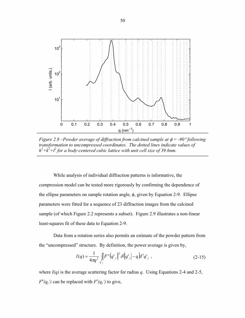
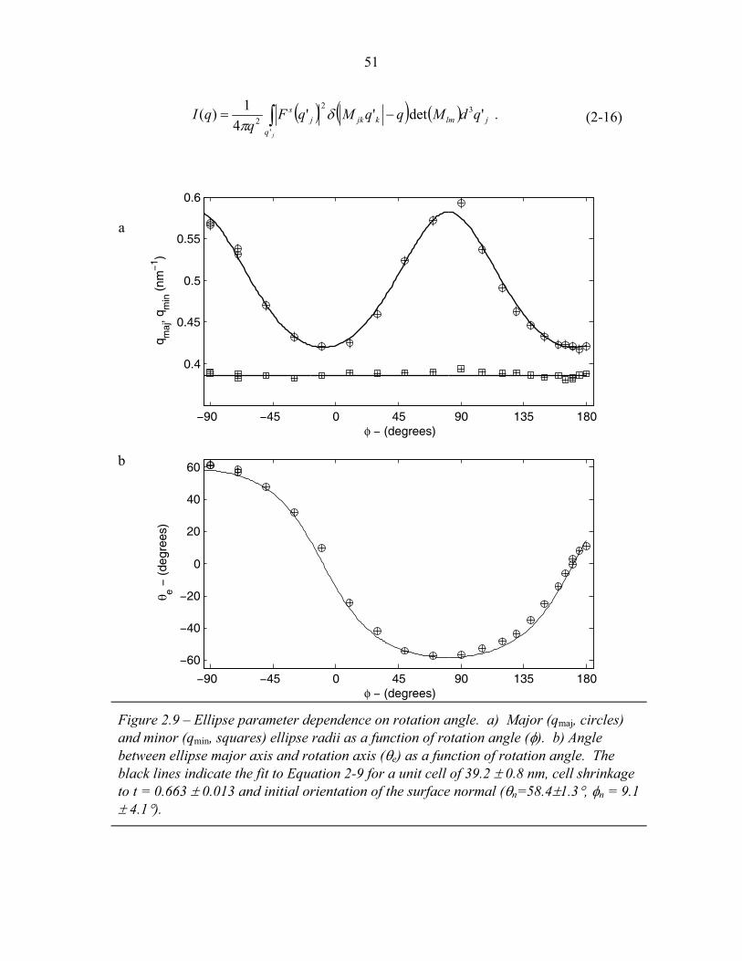
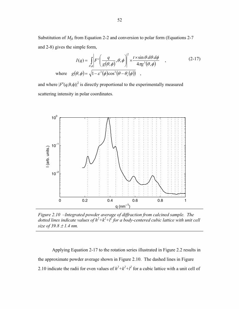
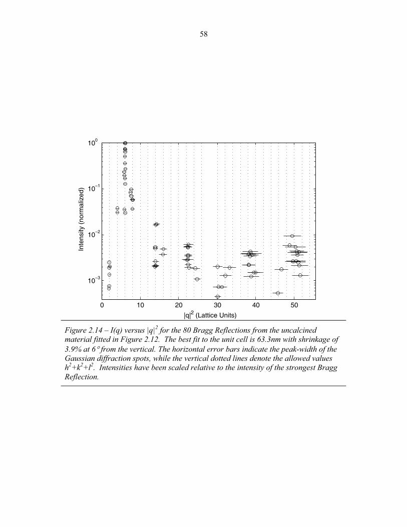
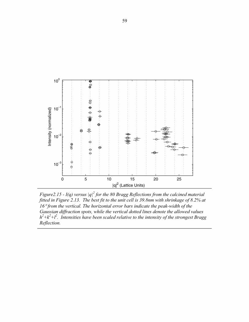
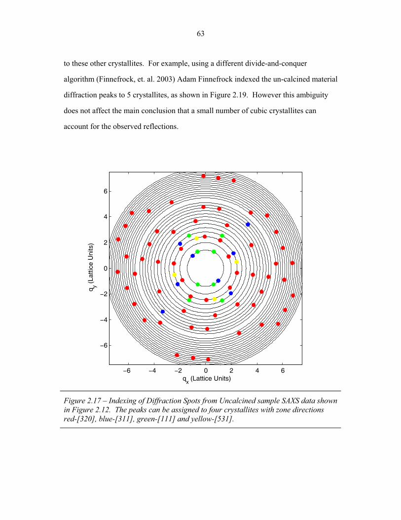
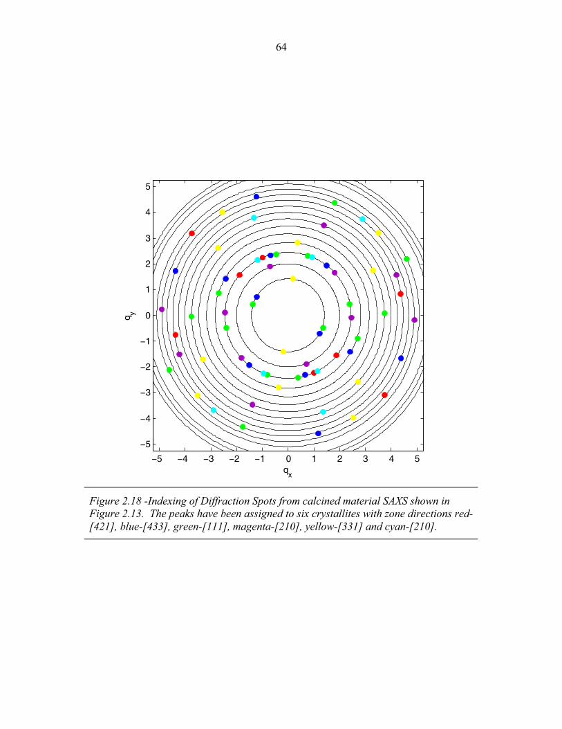
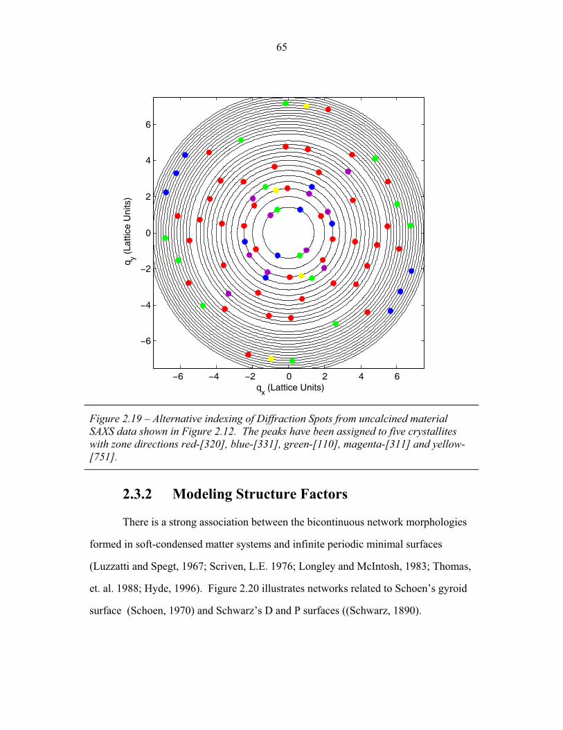
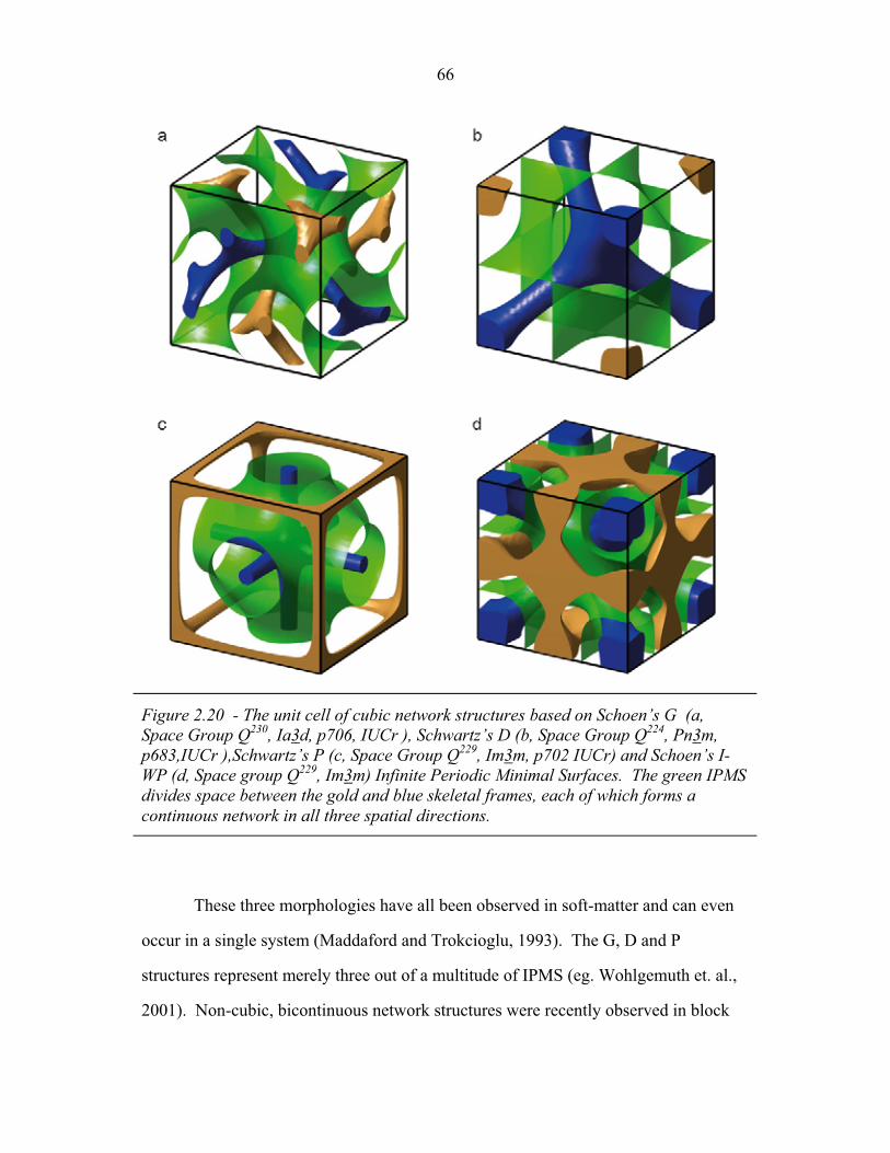
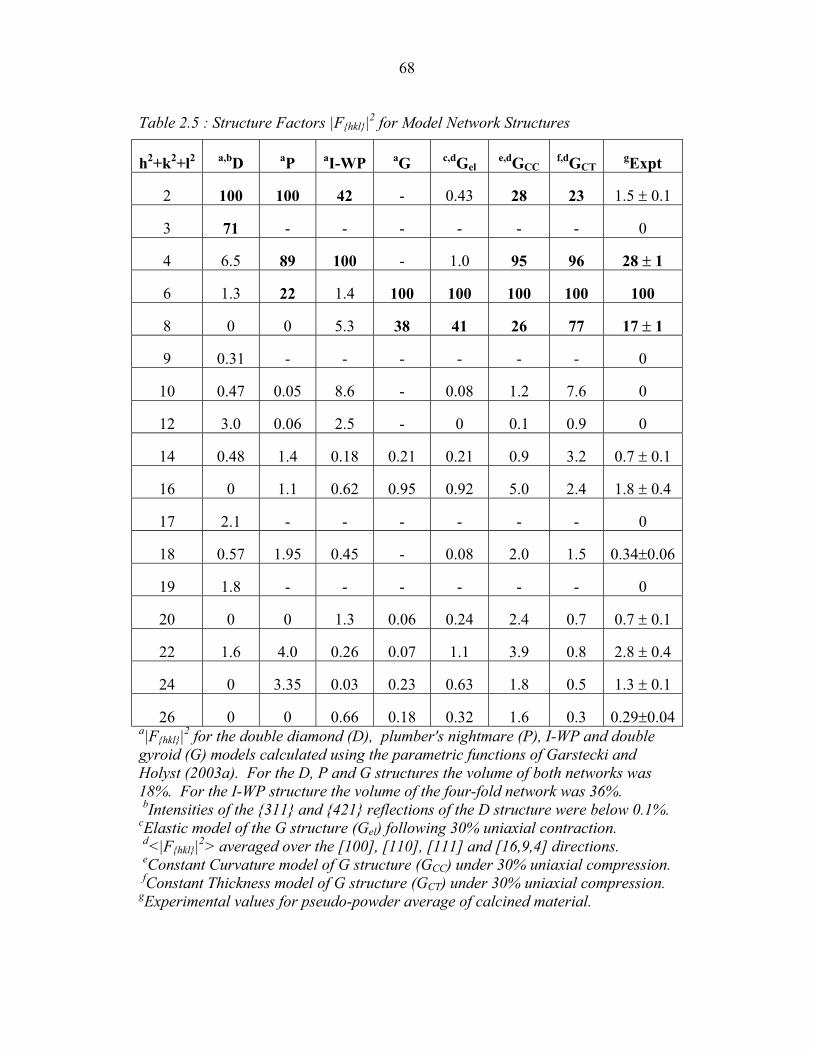
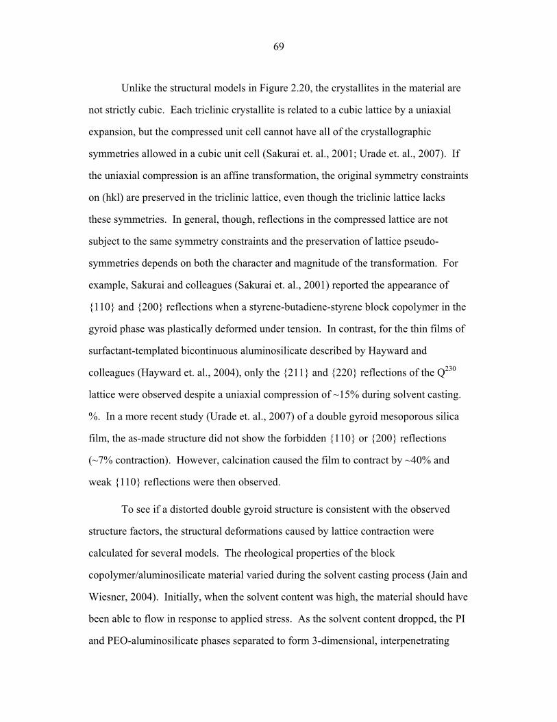
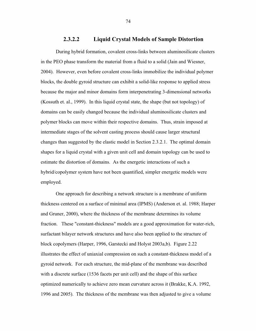
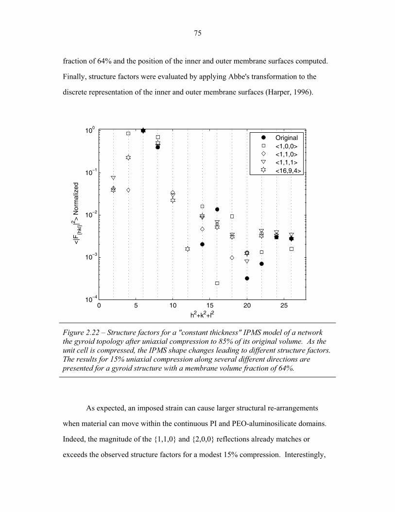
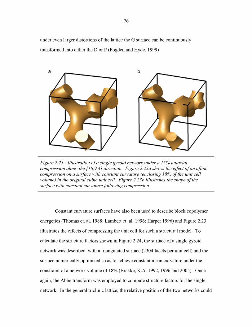
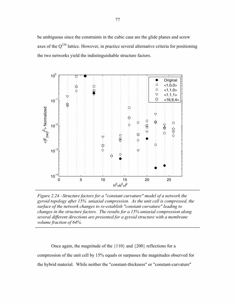
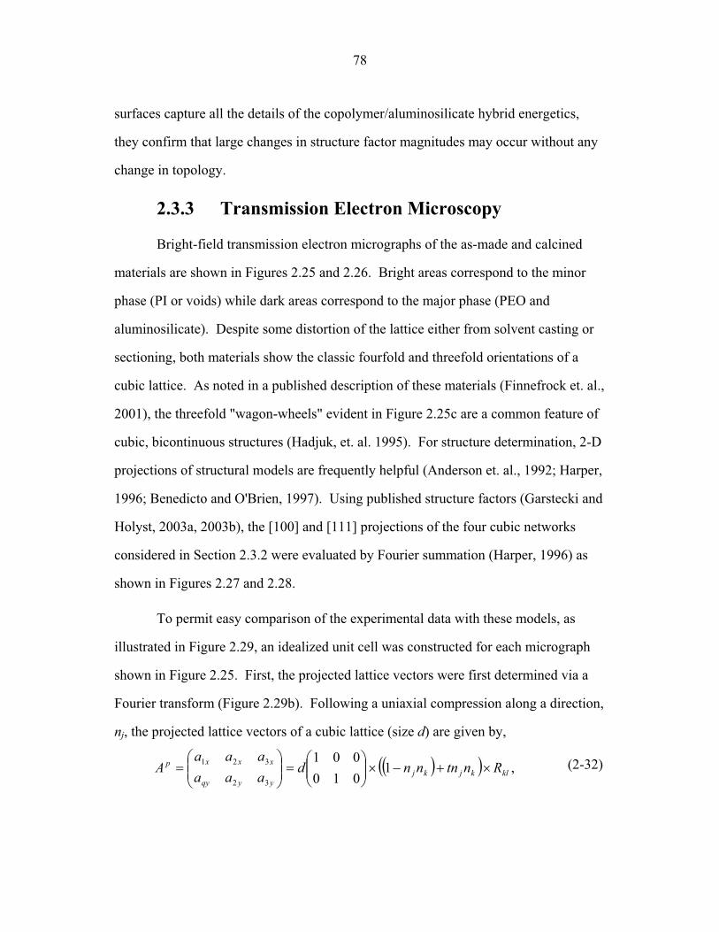
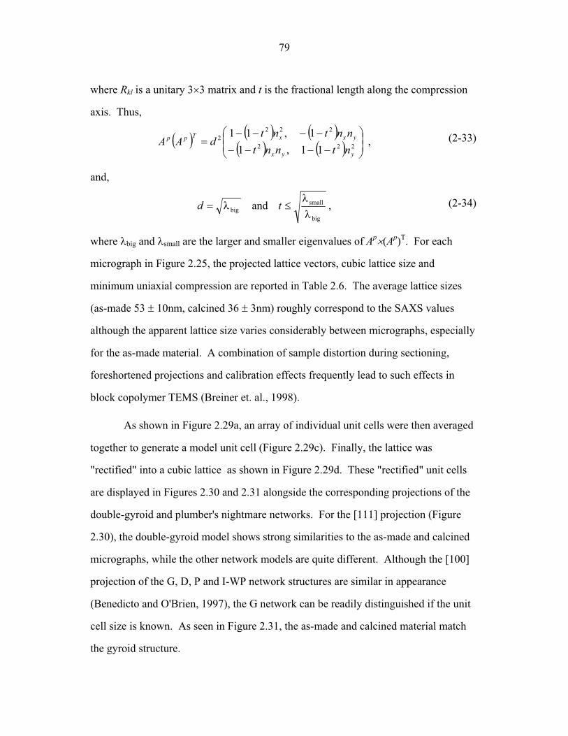
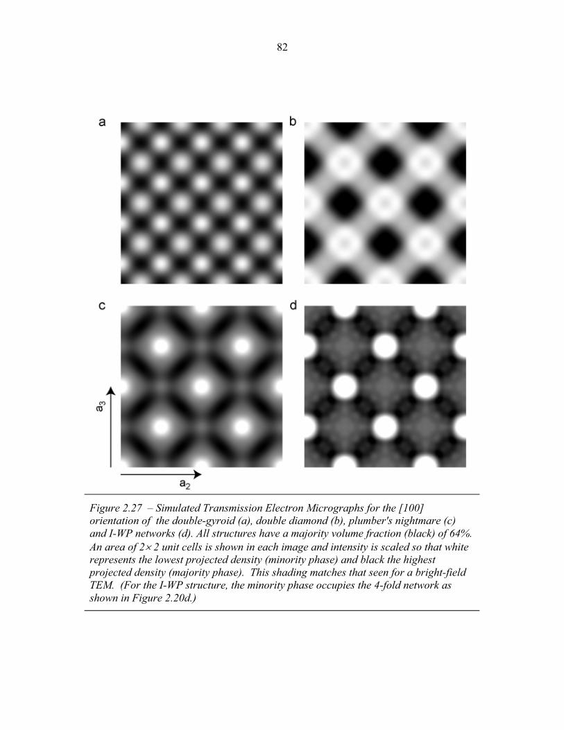
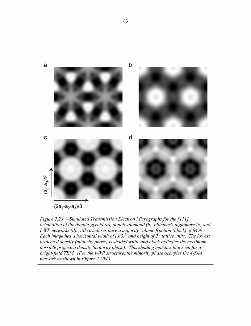
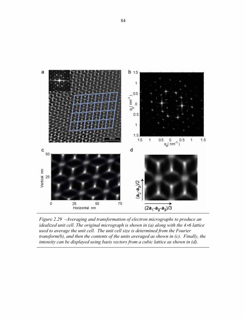
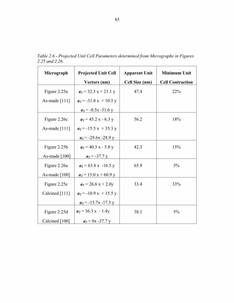
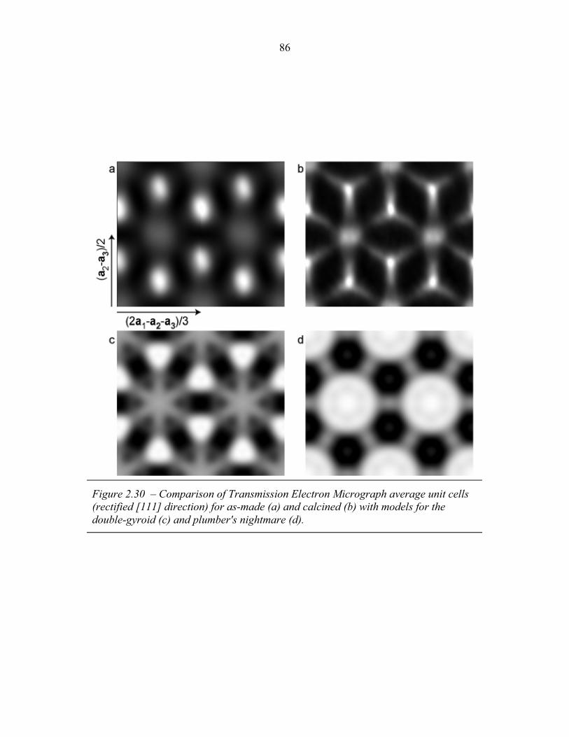
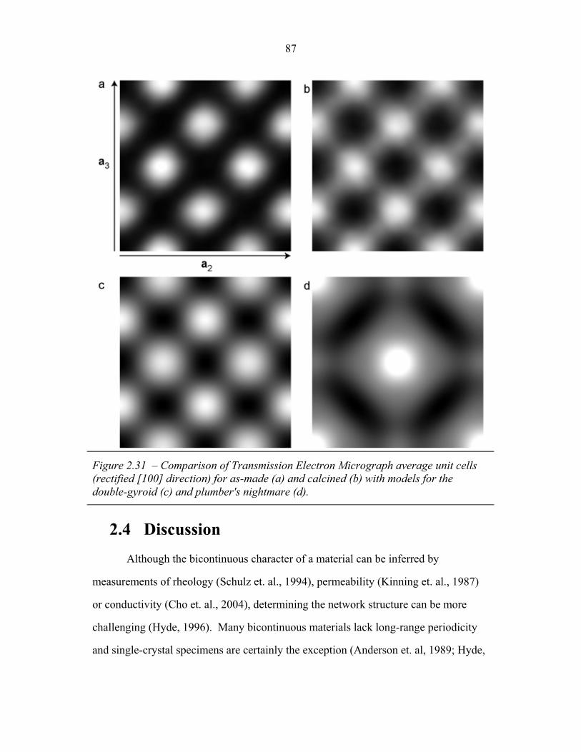
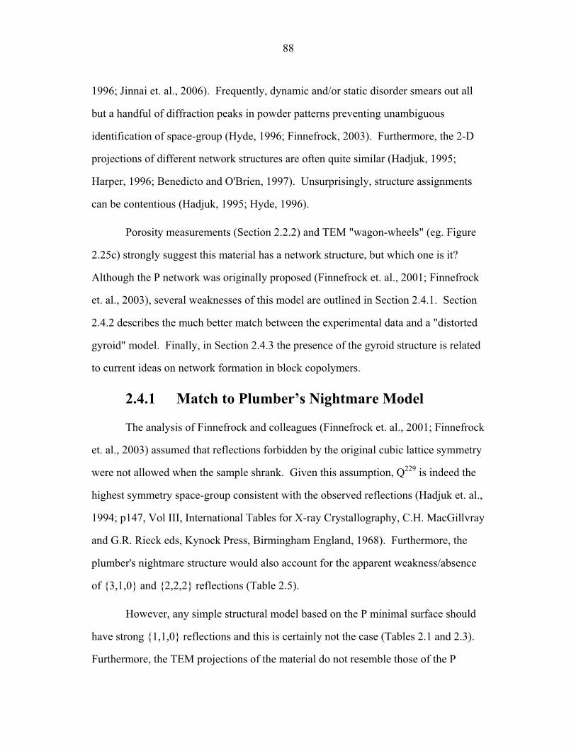
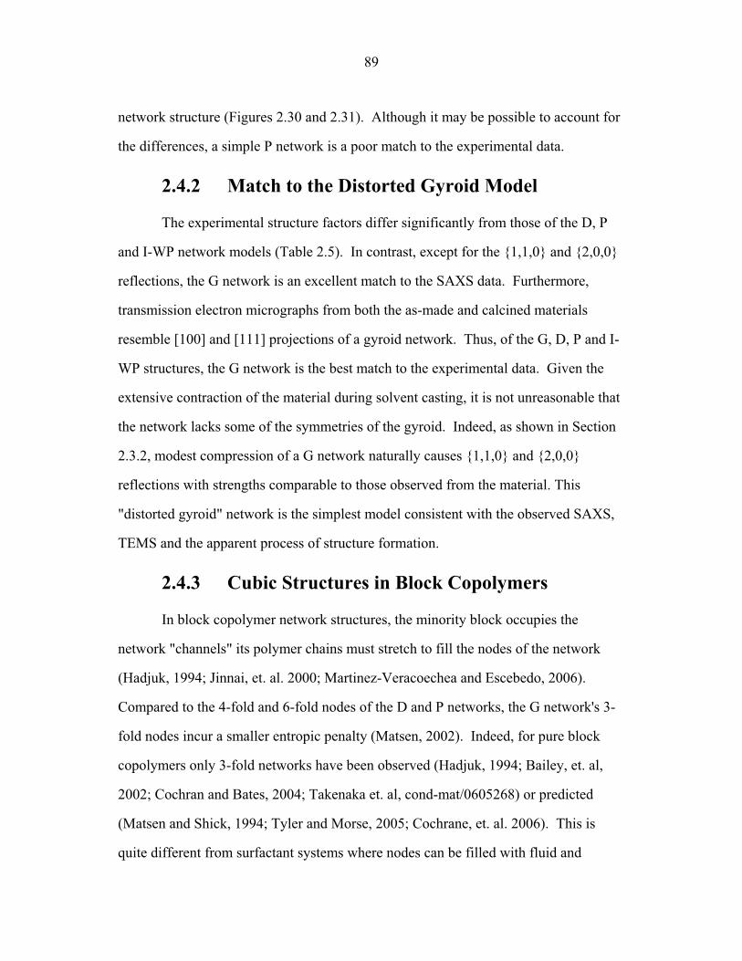
1.1 Block Copolymer Architectures ........................................................... 4 1.2 Disordered, Weakly Segregated and Strongly Segregated States ........ 13 1.3 Diblock Copolymer Morphologies ....................................................... 16 1.4 Domain Interfacial Curvature ............................................................... 17 1.5 ABC Triblock Copolymer Morphologies ............................................. 19 1.6 Structural Templating of Silica with Block Copolymers ..................... 22 1.7 Schematic of Small Angle X-ray Scattering beam line ........................ 25 1.8 Examples of SAXS data ........................................................................ 27 2.1 2-D SAXS images from as-made material ............................................39 2.2 2-D SAXS images for calcined material ............................................... 40 2.3 Deformation in Real and Reciprocal Space .......................................... 42 2.4 Origin of Elliptical Scattering Rings .................................................... 44 2.5 Hand-Fitting of Elliptical Ring Shape .................................................. 46 2.6 Least-Squares Fitting of Elliptical Ring Shape .................................... 48 2.7 Rectification of 2-D SAXS Patterns ..................................................... 49 2.8 Powder Average from Rectified SAXS (calcined) ............................... 50 2.9 Elliptical Parameters as a Function of Rotation Angle ......................... 51 2.10 Rotational Powder Average SAXS of Calcined Material ..................... 52 2.11 Rotational Powder Average SAXS of As-Made Material .................... 55 2.12 2-D SAXS Image from As-Made Material ........................................... 56 2.13 2-D SAXS from Calcined Material ....................................................... 57 2.14 Plot of I versus |q|2 for Bragg Spots of As-Made Diffraction ............... 58 2.15 Plot of I versus |q|2 for Bragg Spots of Calcined Diffraction ................59 2.16 Hand Indexing of Diffraction Spots ...................................................... 61 2.17 Indexed Spots from As-Made Material ................................................ 63 2.18 Indexed Spots from Calcined Material ................................................. 64 2.19 Alternate Indexing of As-Made Material ............................................. 65 2.20 Skeletal Models of the bicontinuous network structures ...................... 66 2.21 Structure Factors for Elastic Model of Distorted Double Gyroid ........ 73 2.22 Structure Factors for Constant Thickness Model of Distorted Double Gyroid ...................................................................................... 75 2.23 Affine and Constant Curvature Models of Compressed Double Gyroid ................................................................................................... 76 2.24 Structure Factors for Constant Curvature Model of Distorted Double Gyroid ...................................................................................... 77 2.25 Bright-Field TEM Images of As-Made and Calcined Material ............ 80 2.26 Bright-Field TEM Images of the As-Made Material ............................ 81 2.27 Simulated [100] Projections for Network Structures ........................... 82 2.28 Simulated [111] Projections for Network Structures ........................... 83 2.29 Averaging and Rectification of Micrographs ....................................... 84 2.30 Comparison of [111] Projections .......................................................... 86 2.31 Comparison of [100] Projections .......................................................... 87
x
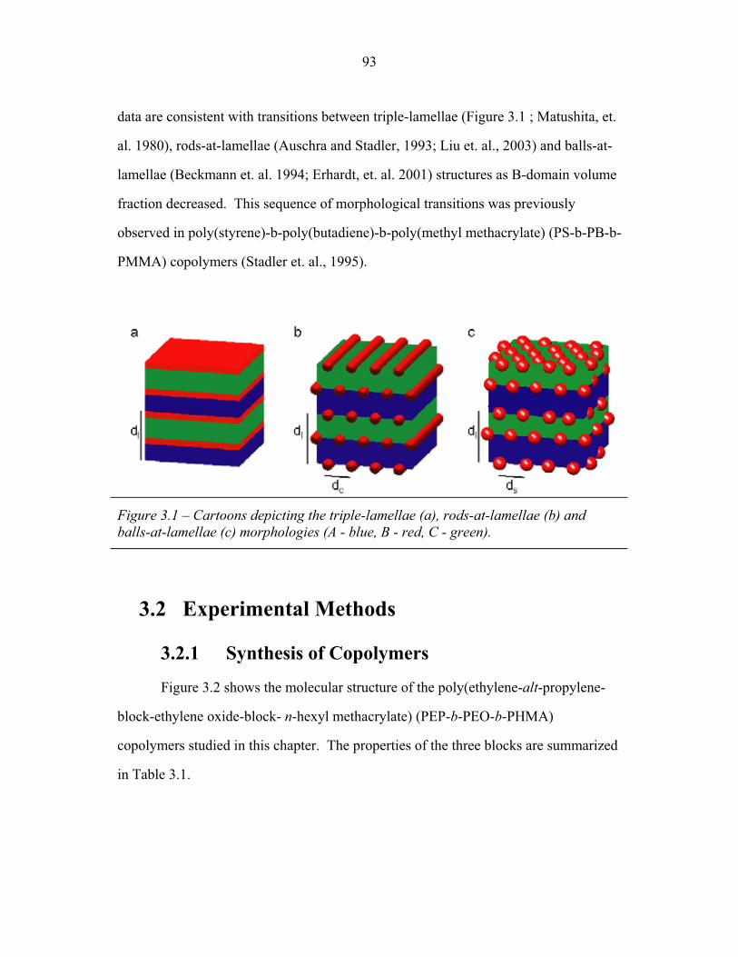
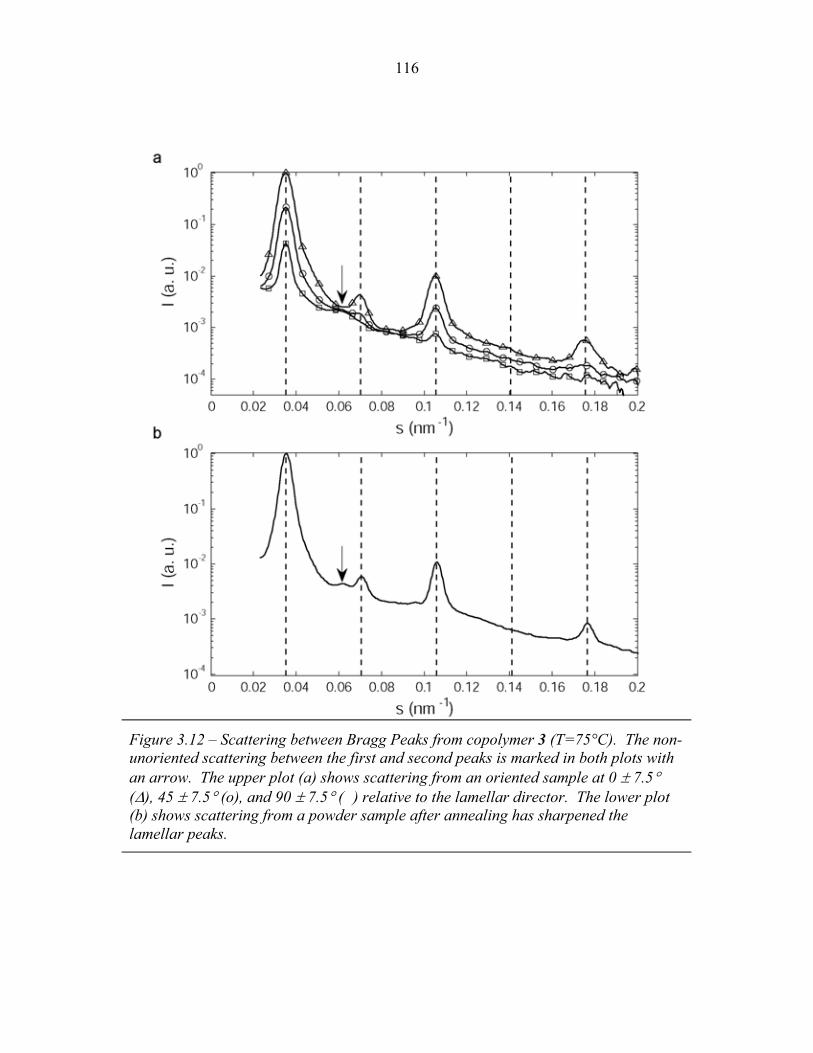
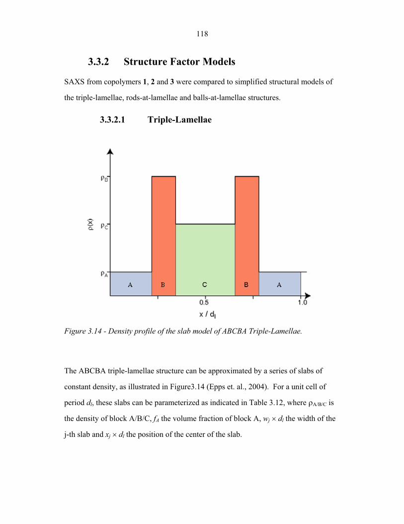
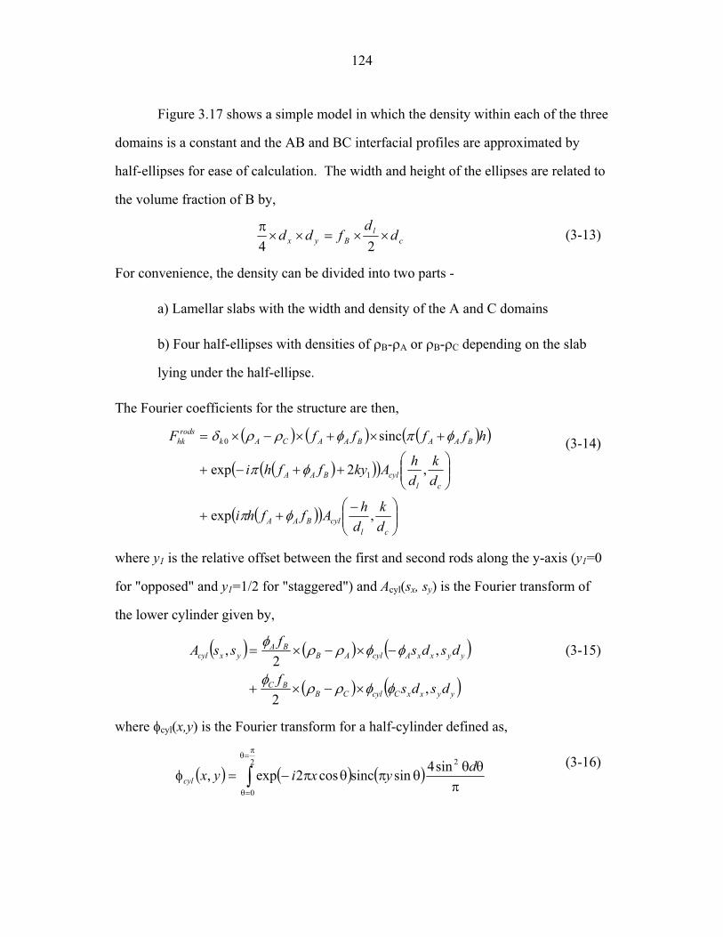
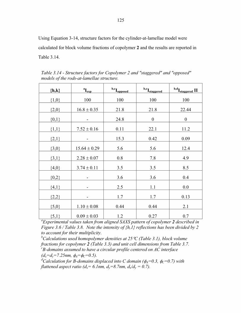
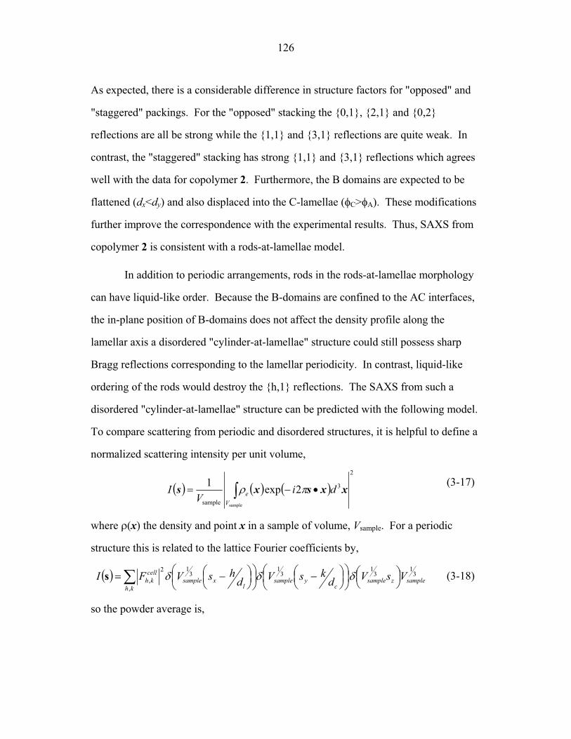
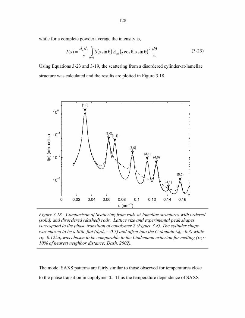
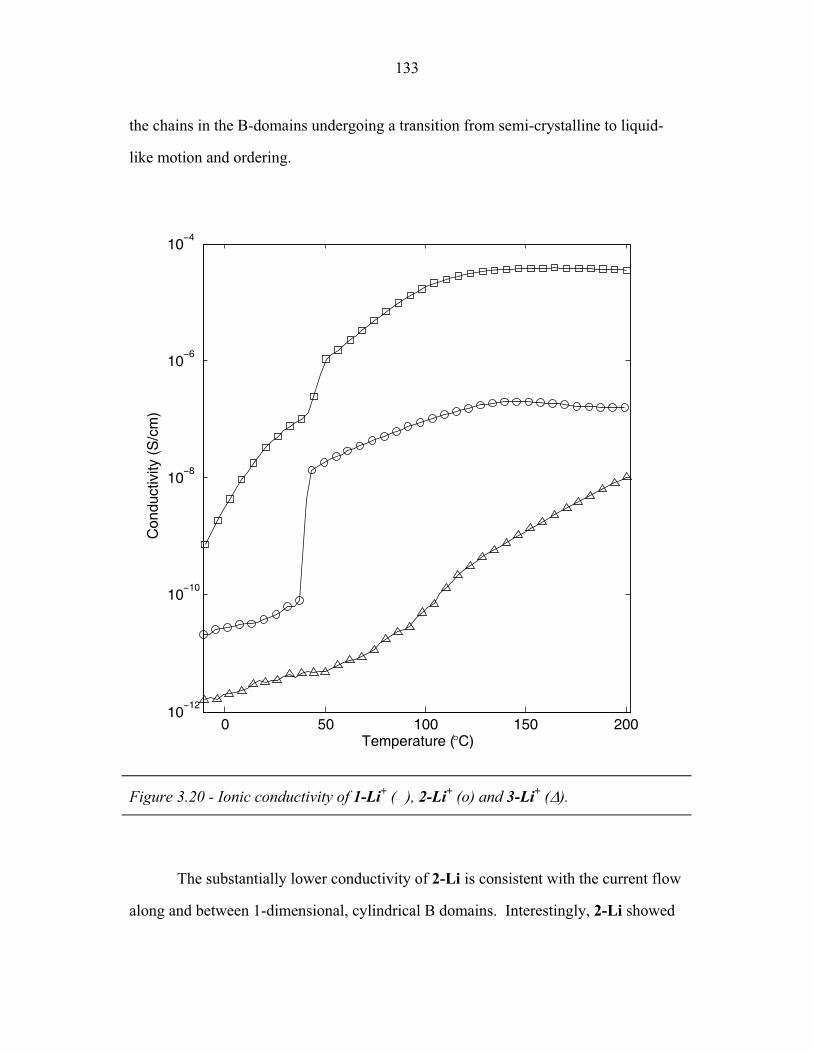
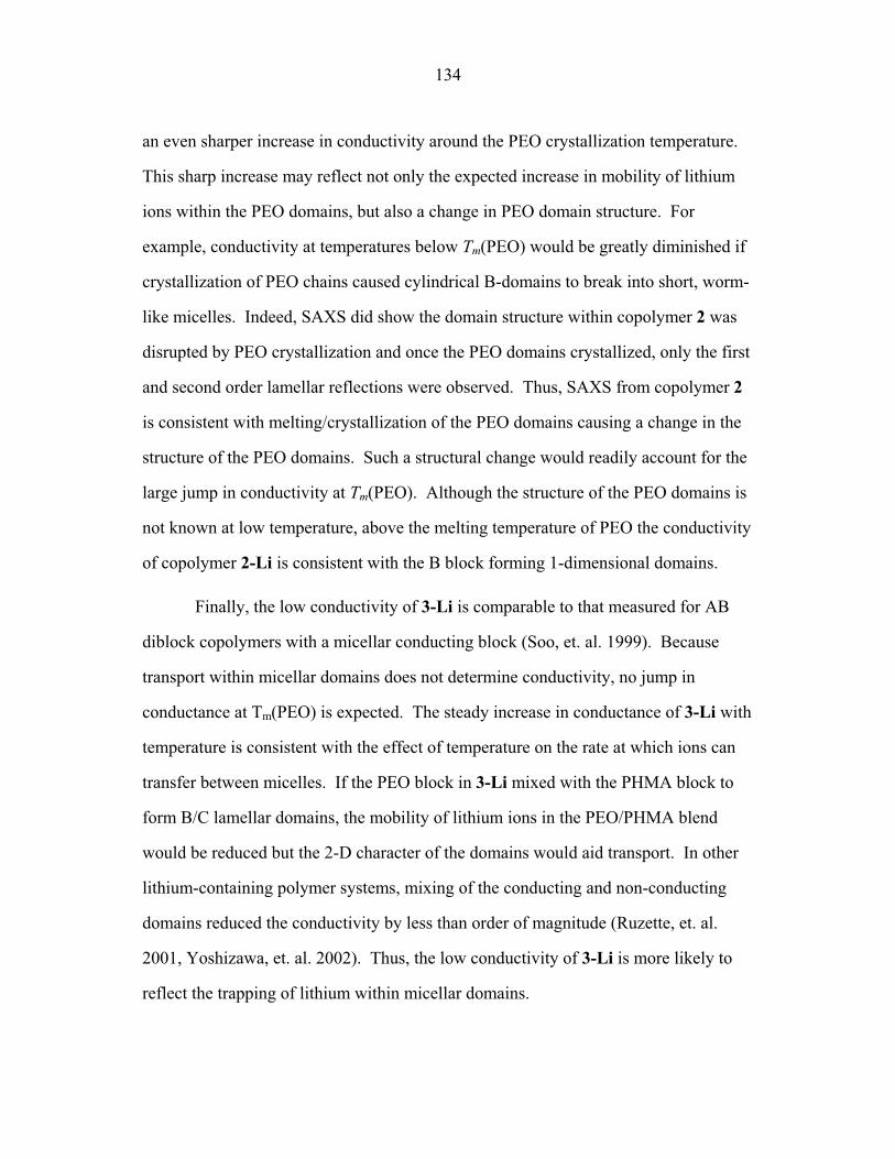
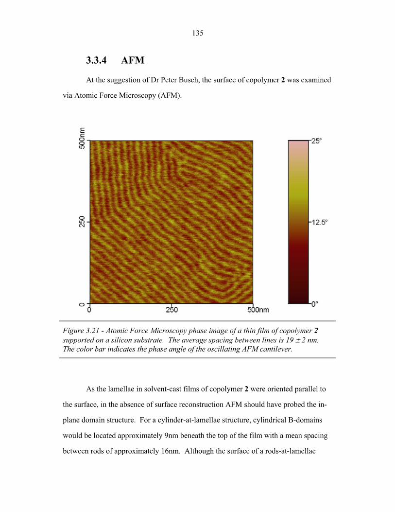
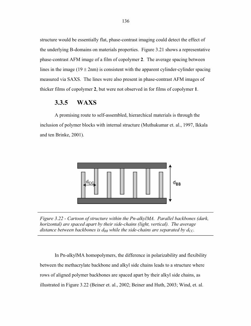
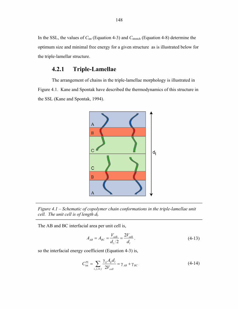
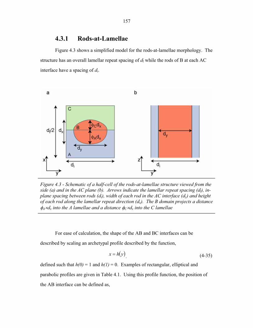
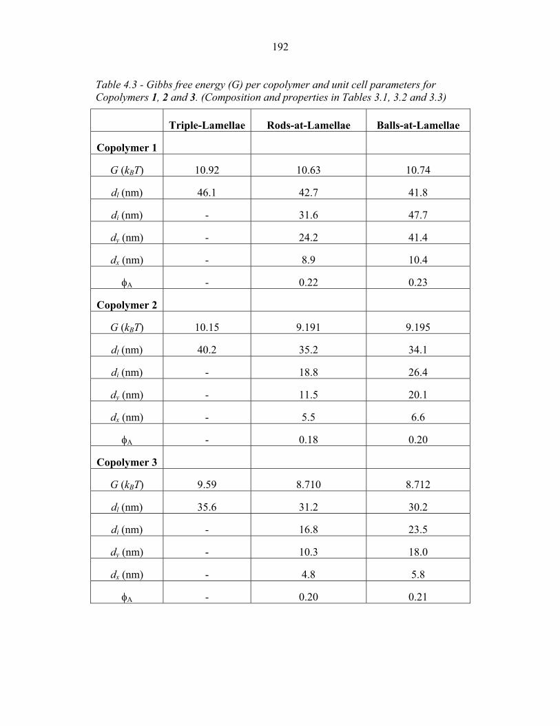
3.1 Cartoons of Triple-Lamellae, Rods-at-Lamellae and Balls-at-Lamellae Structures ................................................................ 93
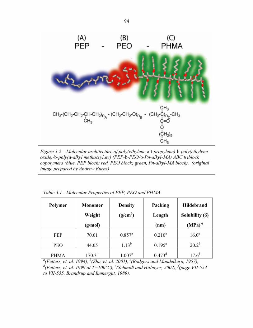
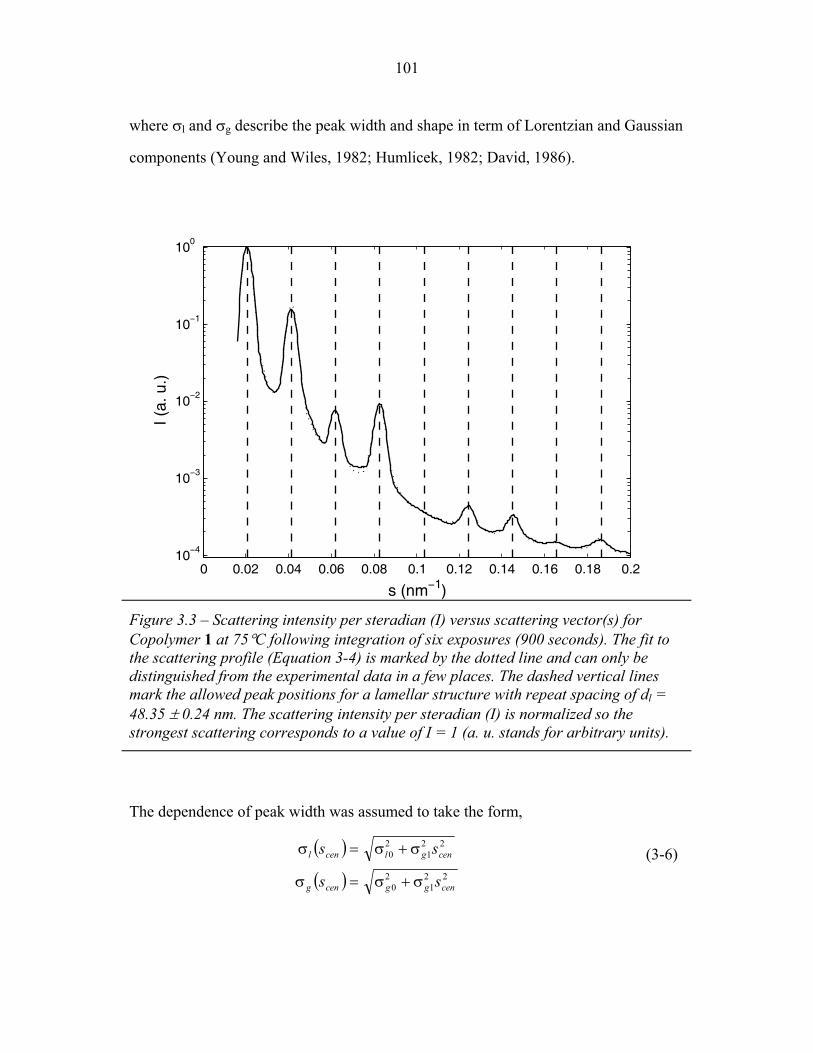
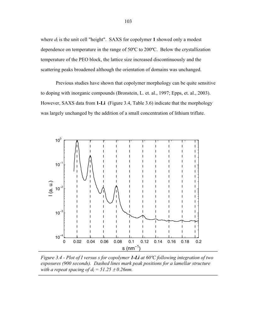
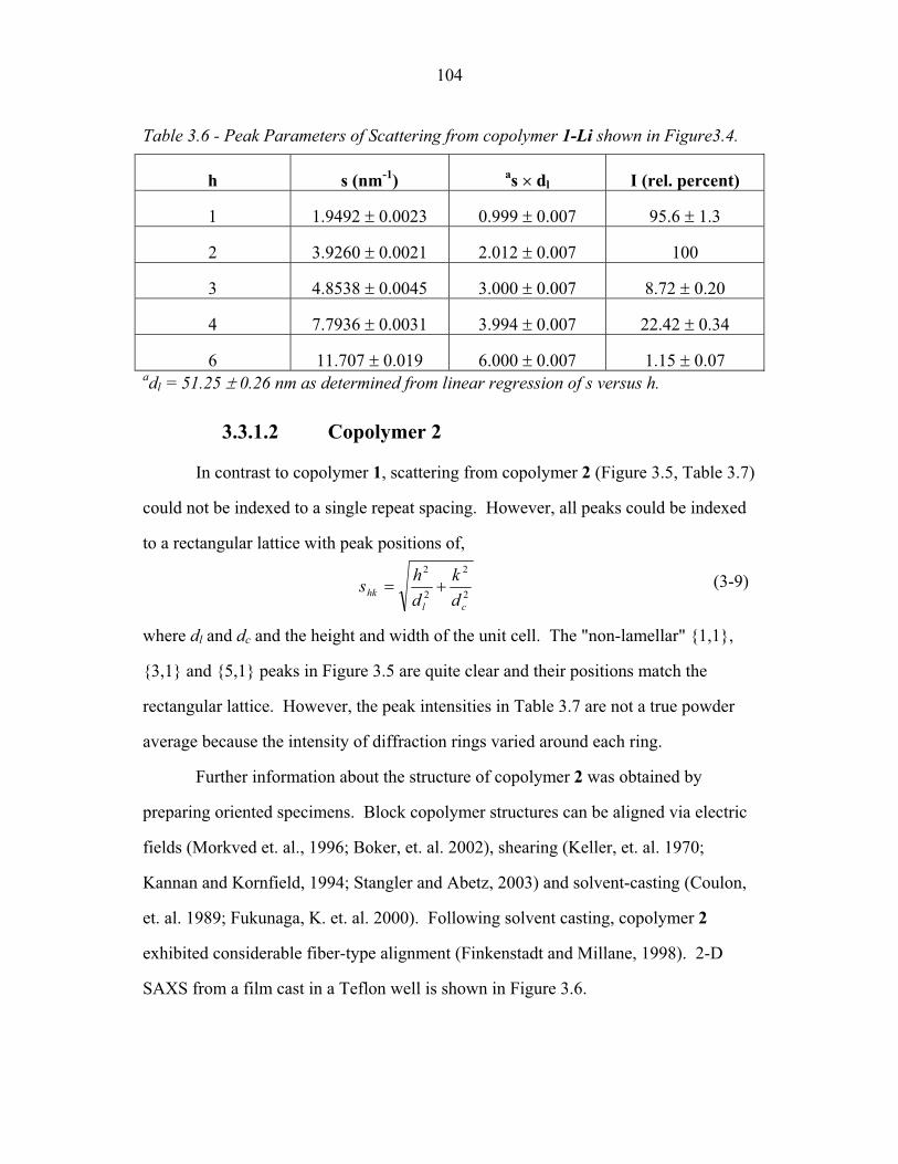
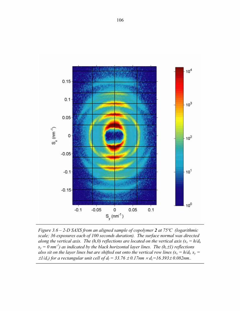
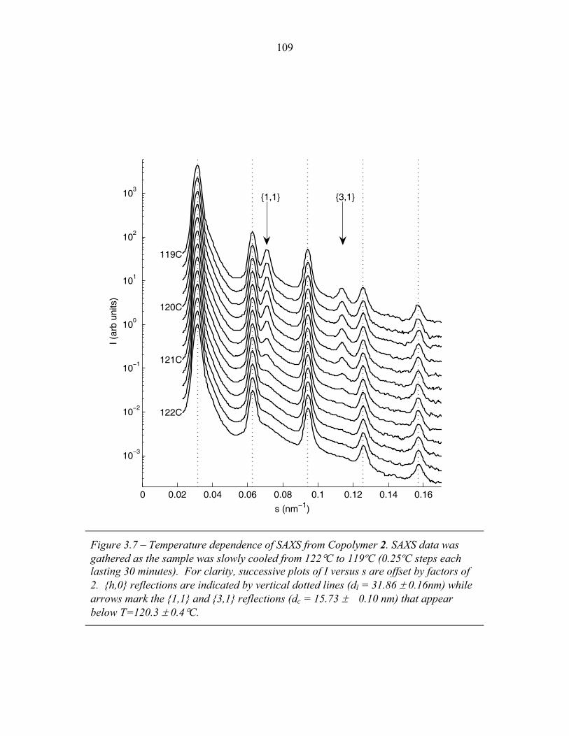
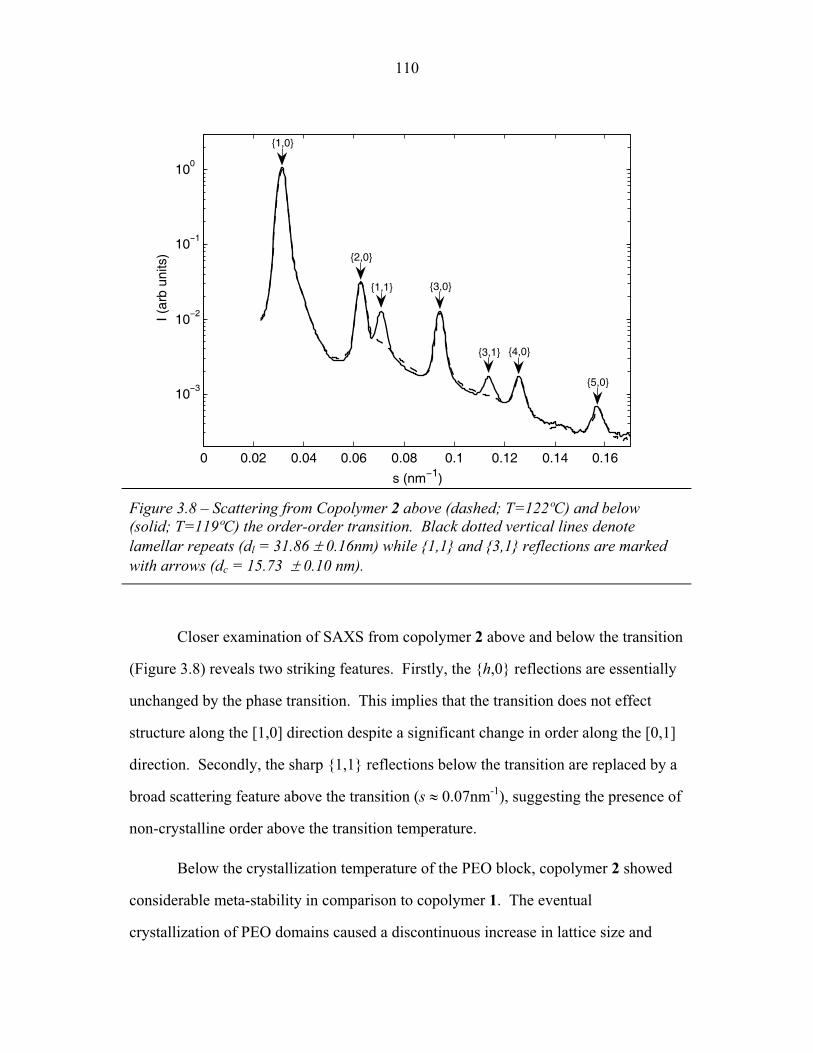
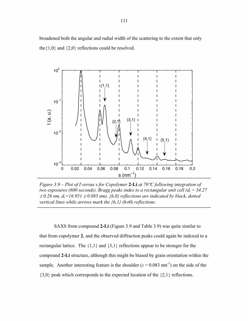
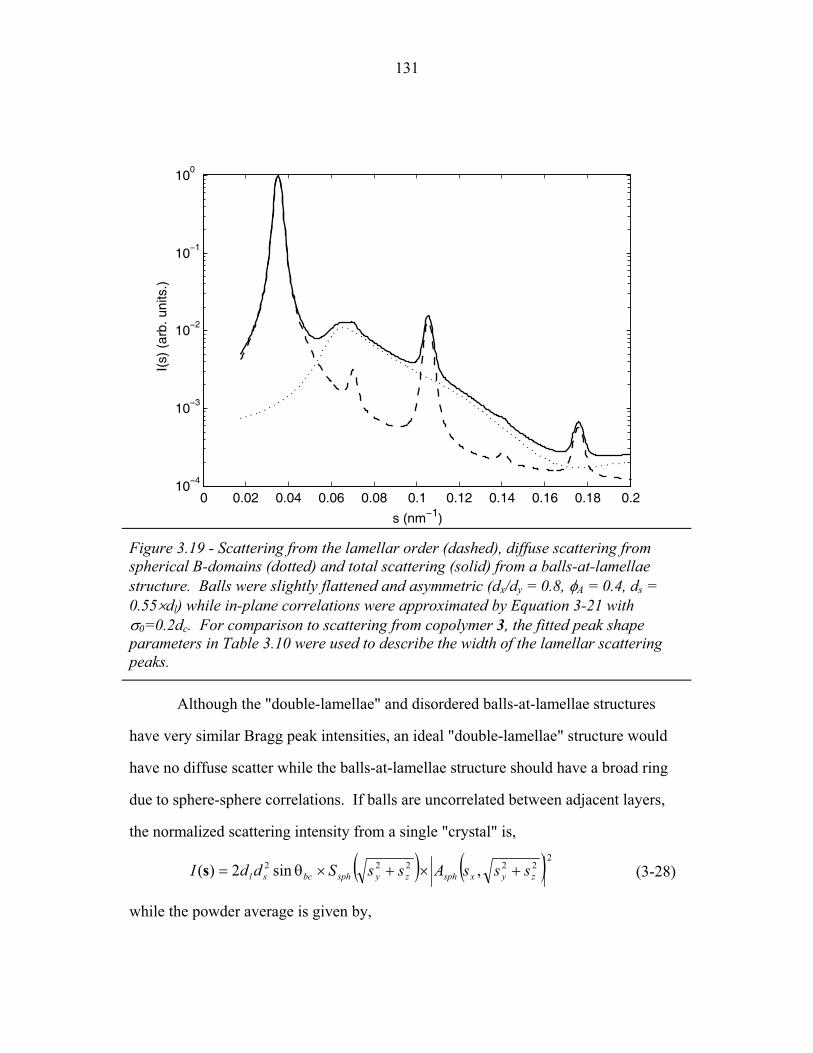
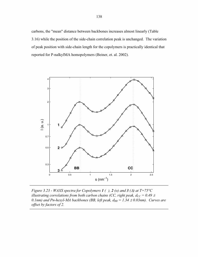
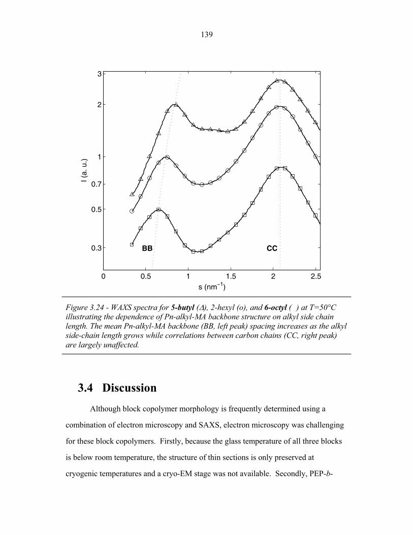
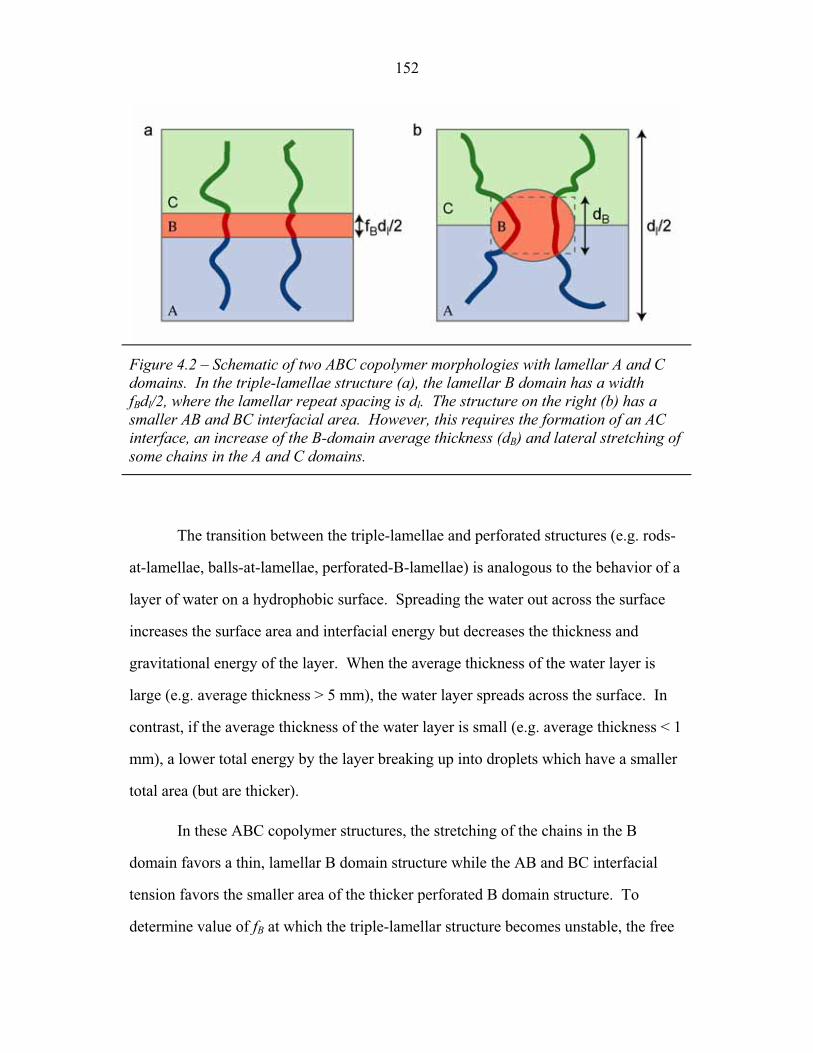
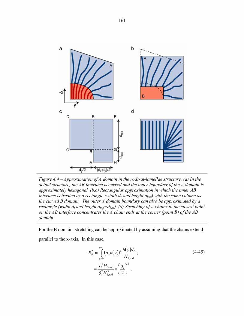
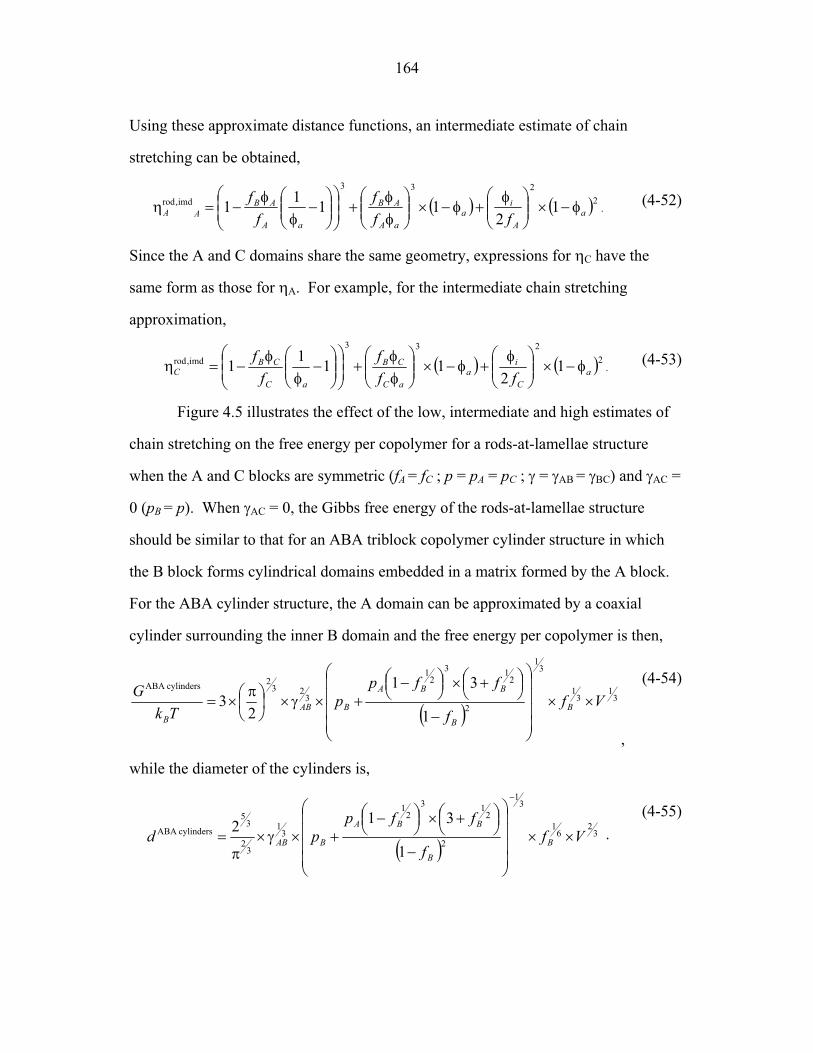
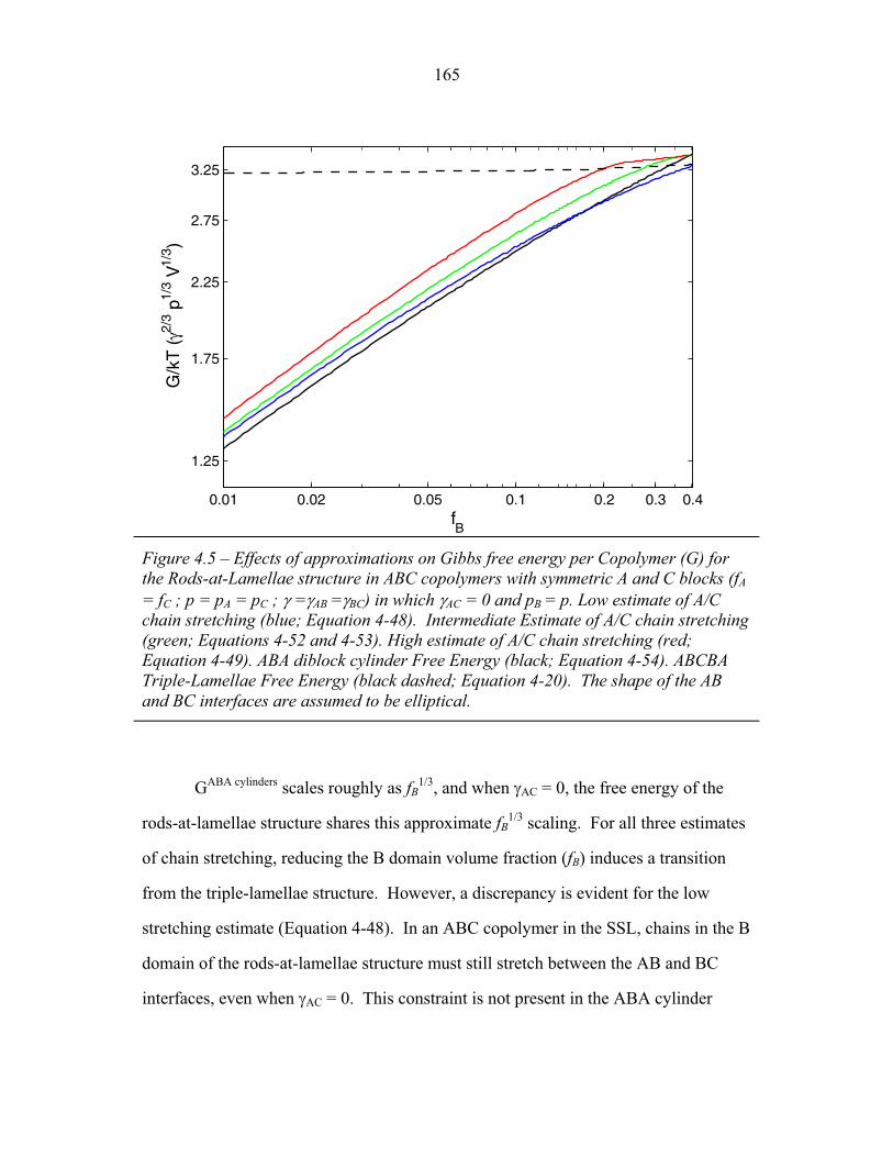
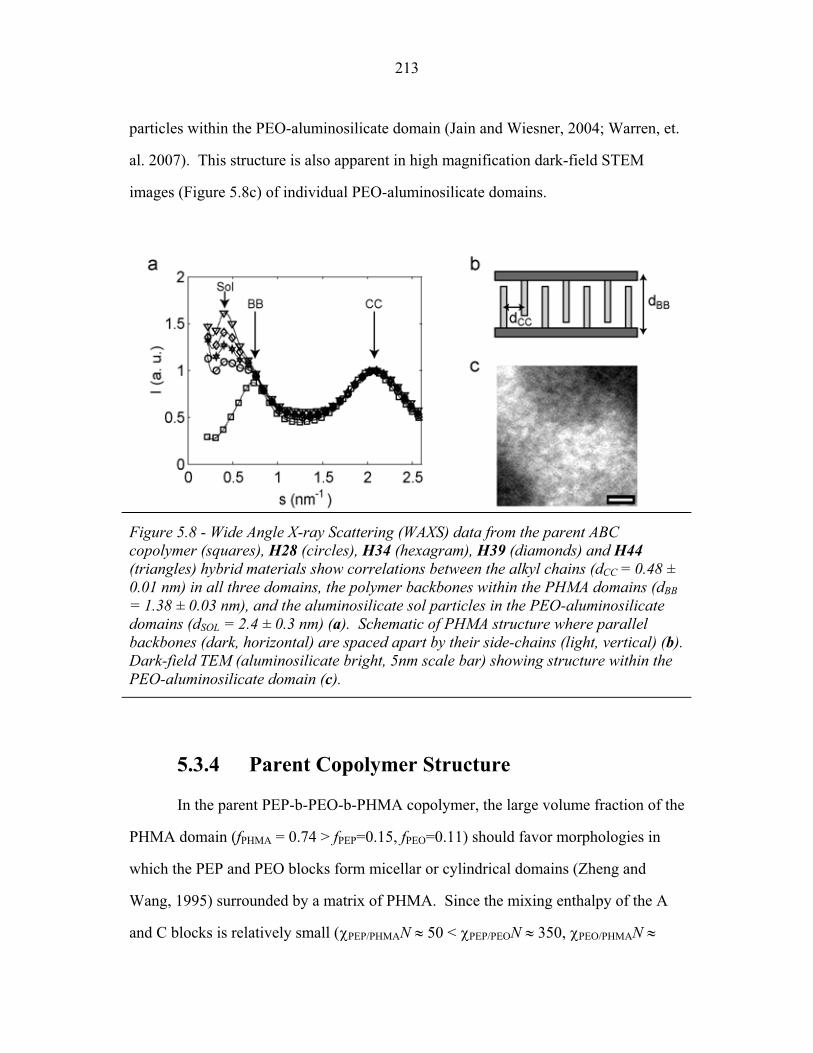
3.2 Molecular Structure of PEP-b-PEO-b-PHMA ..................................... 94 3.3 I versus s for Copolymer 1 ................................................................... 101 3.4 I versus s for Copolymer 1-Li .............................................................. 103 3.5 I versus s for Copolymer 2 ................................................................... 105 3.6 2-D SAXS from Copolymer 2 .............................................................. 106 3.7 Temperature Dependence of SAXS from Copolymer 2 ....................... 109 3.8 More Temperature Dependent SAXS from Copolymer 2 .................... 110 3.9 I versus s from Copolymer 2-Li ........................................................... 111 3.10 Temperature Dependent SAXS from Copolymer 2-Li ......................... 113 3.11 I versus s from Copolymer 3 ................................................................ 114 3.12 Oriented SAXS from Copolymer 3 ...................................................... 116 3.13 I versus s from Copolymer 3-Li ........................................................... 117 3.14 Slab model of Triple-Lamellae Structure ............................................. 118 3.15 Reconstructed Density Profile for Copolymer 1 .................................. 121 3.16 Staggered and Opposed Chain Packing in the Rods-at-Lamellae Structure ................................................................................................ 122 3.17 Rods-at-Lamellae Electron Density Model .......................................... 123 3.18 Calculated Powder Scattering for Rods-at-Lamellae Structure ............ 128 3.19 Calculated Powder Scattering for Balls-at-Lamellae Structure ............ 131 3.20 Ionic Conductivity of Copolymers 1-Li+, 2-Li+ and 3-Li+ ...................133 3.21 AFM Image of Copolymer 2 ................................................................. 135 3.22 Backbone and Side-chain structure in the PHMA ................................ 136 3.23 WAXS from Copolymers 1, 2 and 3 .................................................... 138 3.24 WAXS from Copolymer 5-butyl and 6-octyl. ..................................... 139 4.1 Chain Conformations in the Triple-Lamellae Structure ....................... 148 4.2 Interfacial Instability ............................................................................ 152 4.3 Rods-at-Lamellae Schematic ............................................................... 157 4.4 Box Approximation for Chain Stretching ............................................ 161 4.5 Effect of Chain Stretching Approximation on Gibbs Free Energy of Rods-at-Lamellae Structure ............................................................. 165 4.6 Effect of Other Approximations on Gibbs Free Energy of
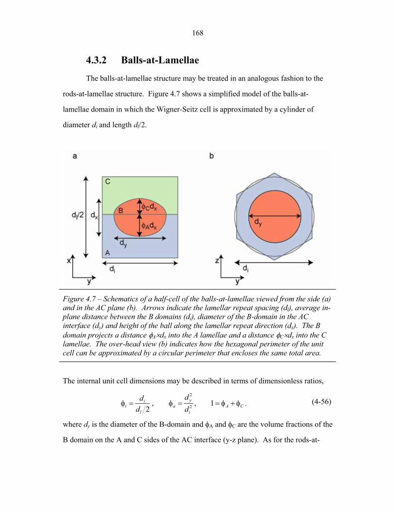
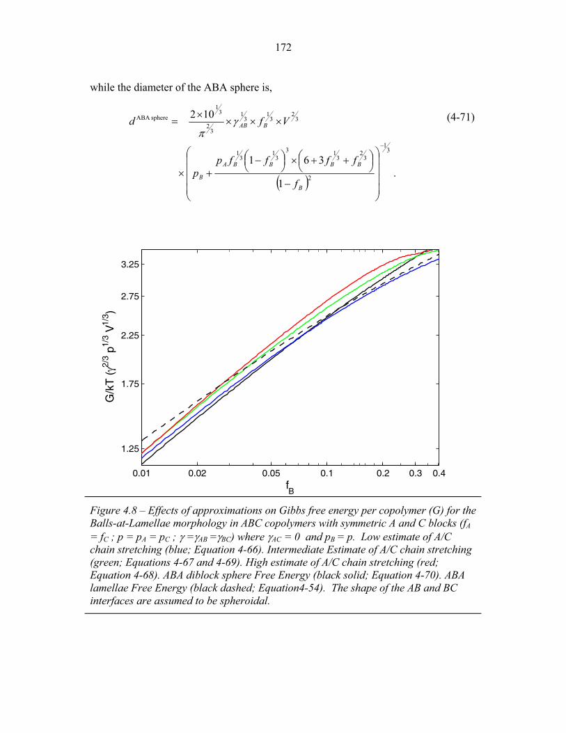
of Rods-at-Lamellae Structure ............................................................. 167 4.7 Balls-at-Lamellae Schematic ............................................................... 168 4.8 Effect of Chain Stretching Approximation on Gibbs Free Energy
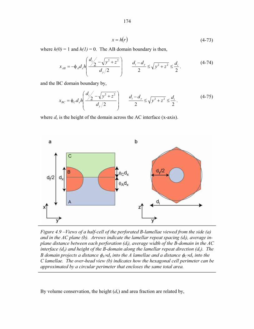
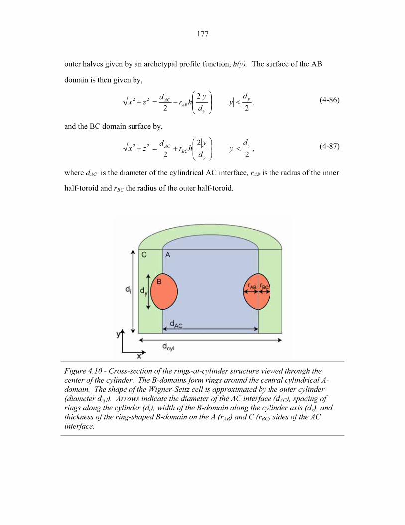
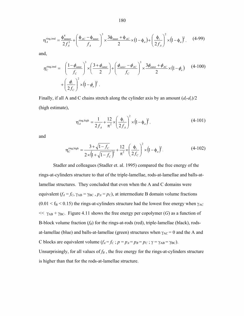
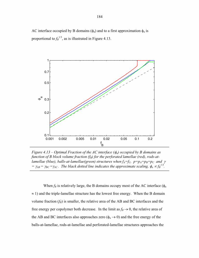
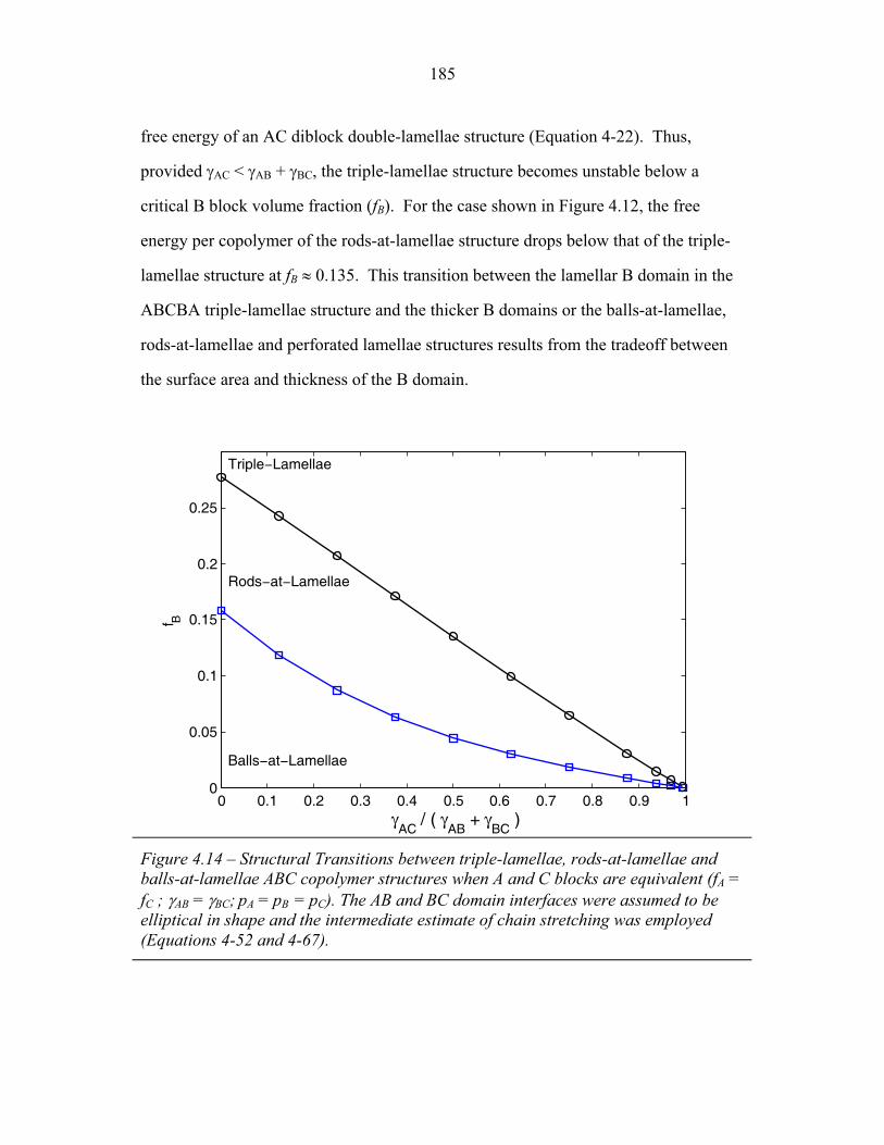
of Balls-at-Lamellae Structure ............................................................. 172 4.9 Perforated-Lamellae Schematic ........................................................... 174 4.10 Rings-at-Lamellae Schematic .............................................................. 177 4.11 Gibbs Free Energy versus Composition for Rings-at-Lamellae .......... 181 4.12 Gibbs Free Energy versus Composition for Triple-Lamellae, Perforated-Lamellae, Rods-at-Lamellae and Balls-at-Lamellae .......... 183 4.13 AC Interfacial Area Fraction versus Composition ............................... 184 4.14 Phase Diagram for Triple-Lamella, Rods-at-Lamellae and Spheres-at-Lamellae ............................................................................. 185
xi
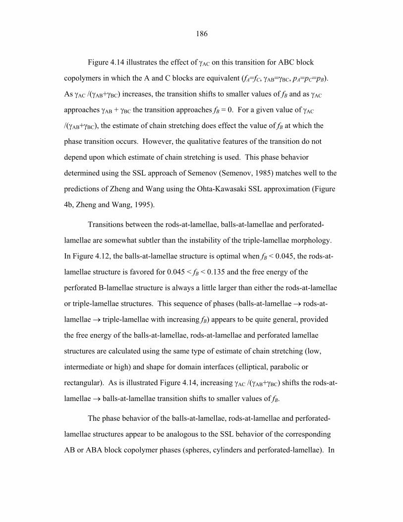
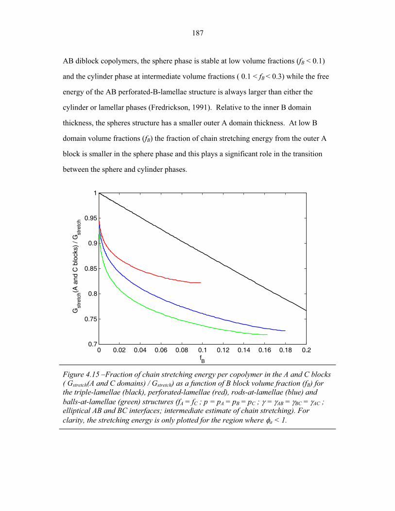
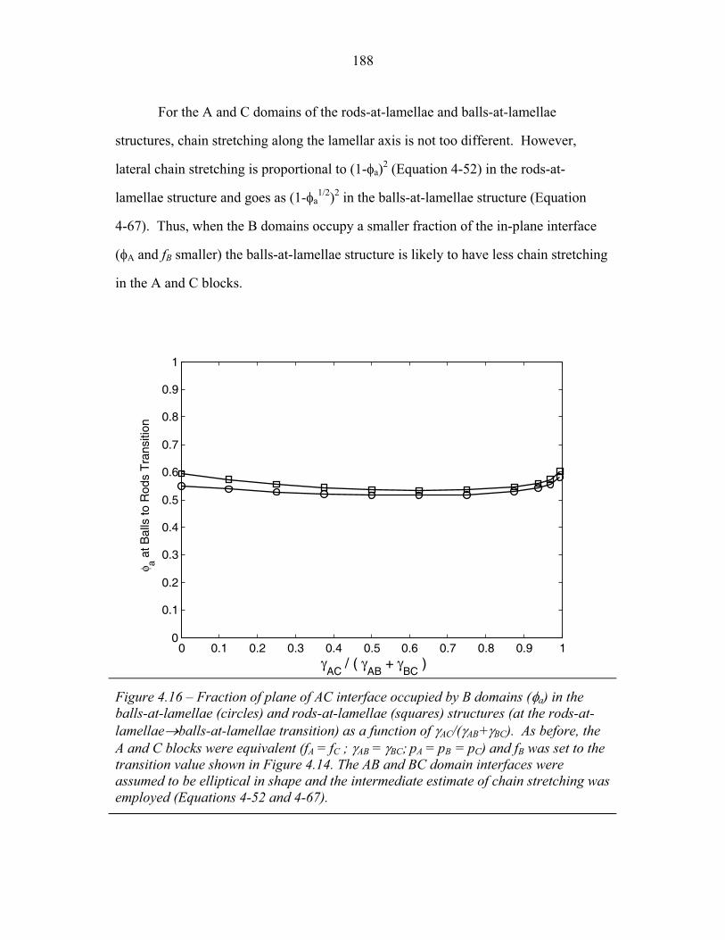
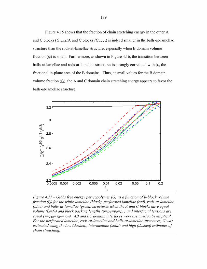
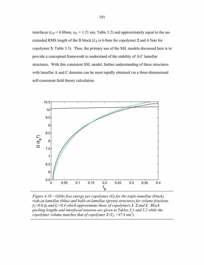
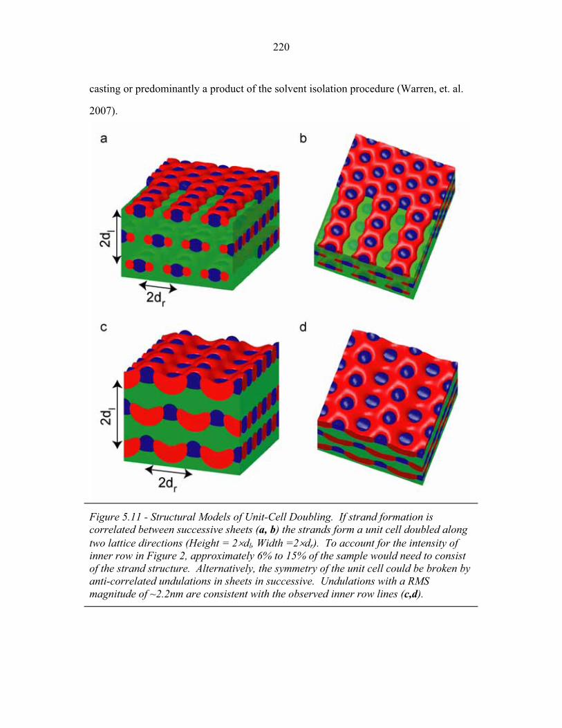
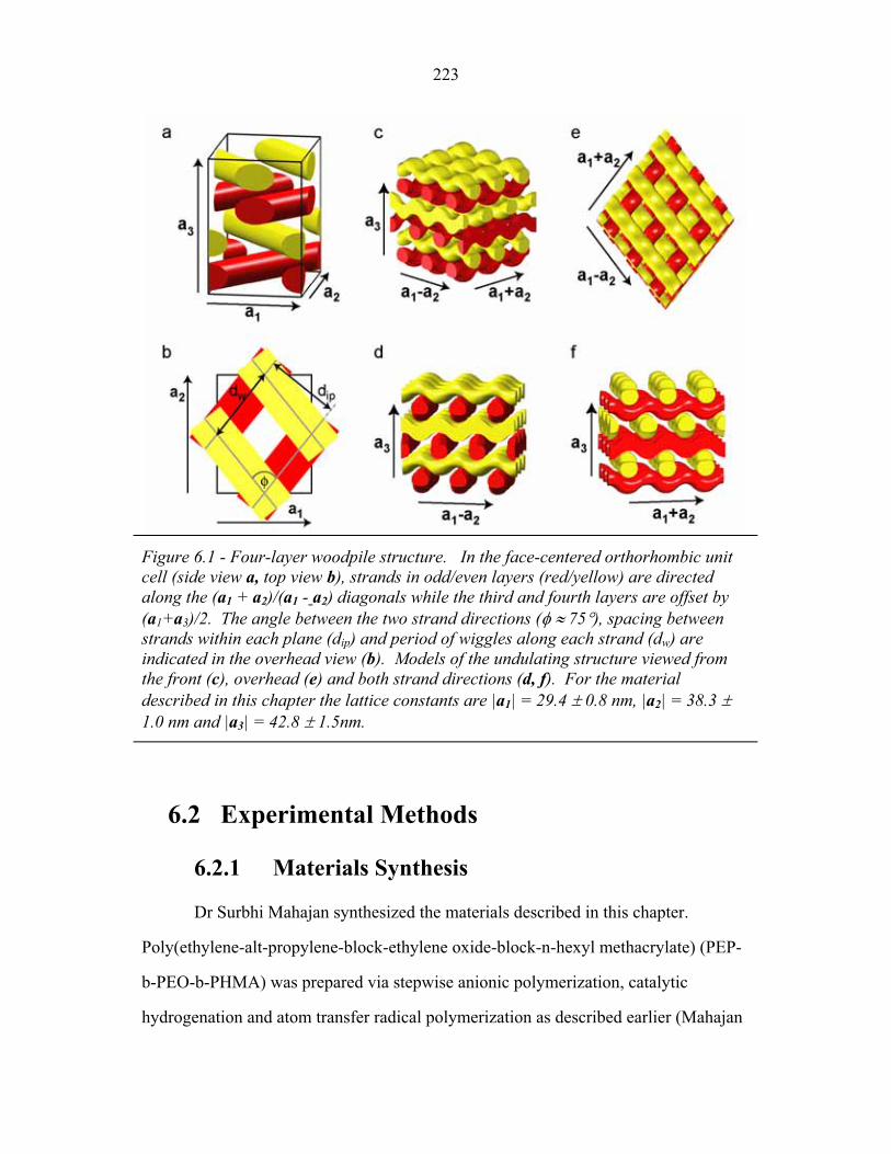
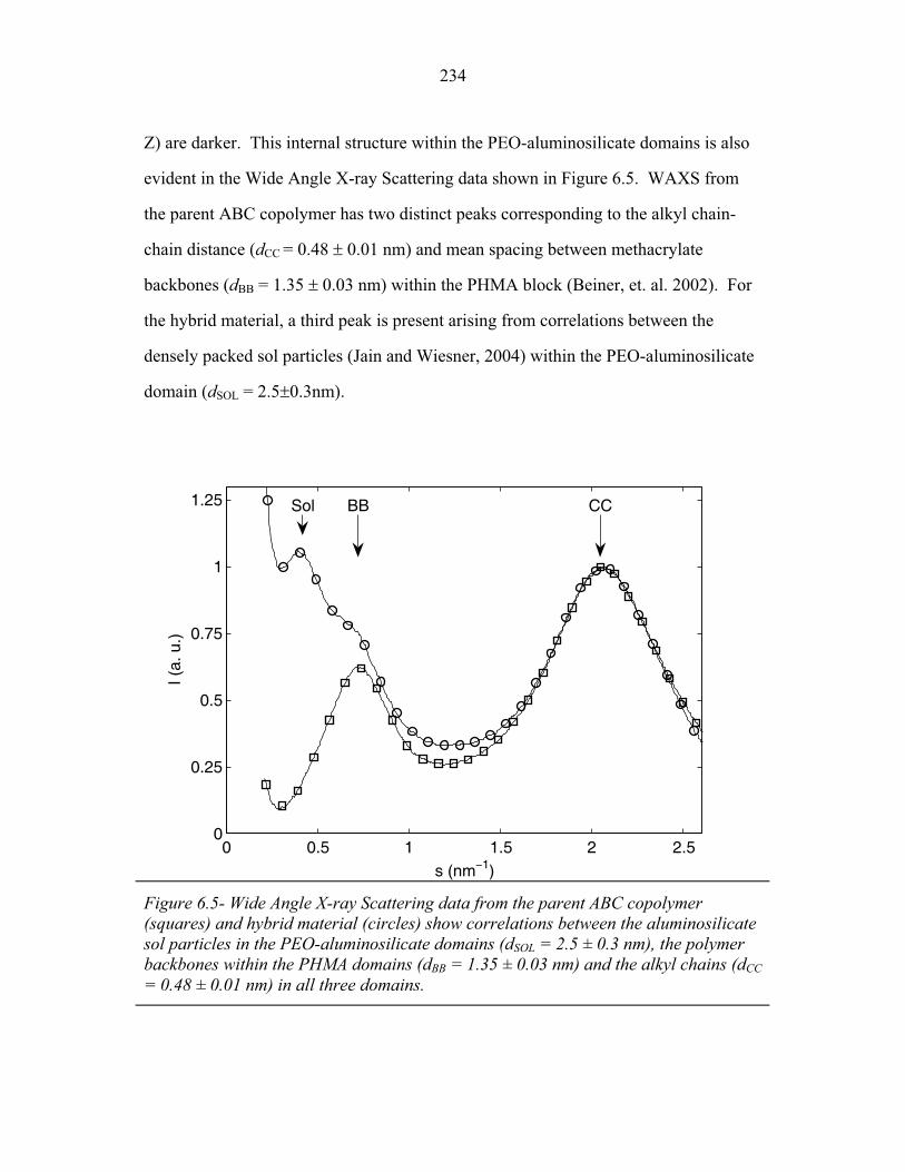
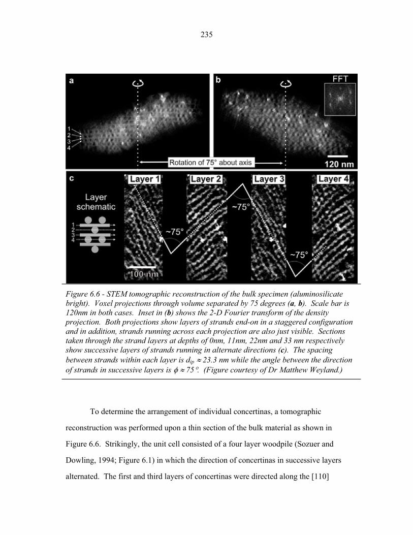
4.15 Fraction of Chain Stretching Energy in AC domains versus Composition ......................................................................................... 187 4.16 Fraction of AC Interface Occupied by B-domains at the Rods � Balls Transition ...................................................................... 188 4.17 Effect of Modeling Approximations on Phase Transitions .................. 189 4.15 Free Energy versus Composition for Copolymers 1, 2 and 3 ............... 191 5.1 Models of ABC Lamellar Structures with small A block ..................... 195 5.2 2-D SAXS from Compound H34 ......................................................... 202 5.3 Hybrid Material Anisotropy ................................................................. 205 5.4 Electron Micrographs of Compound H34 ............................................ 207 5.5 AFM of Compound H34 ...................................................................... 208 5.6 SEM and STEM images of Compounds H34 and H44 ........................ 210 5.7 EM Images of Fragmentation of Compounds H34 and H44 ................ 211 5.8 WAXS and EM of Internal Domain Structure ......................................213 5.9 SAXS from Shear-Aligned Sample of Parent Copolymer ....................215 5.10 SAXS from Solvent-Annealed Sample of Parent Copolymer .............. 216 5.11 Structural Models of Unit Cell Doubling ..............................................220 6.1 Four-Layer Woodpile Structure ............................................................223 6.2 SAXS from parent ABC copolymer ..................................................... 229 6.3 SAXS from hybrid material .................................................................. 231 6.4 TEM and Tomographic Reconstruction of Isolated Strand .................. 232 6.5 WAXS ................................................................................................... 234 6.6 Tomographic Reconstruction of Bulk Material .................................... 235 6.7 Generalized Voronoi Cell of the Four-Layer Woodpile Lattice .......... 238 6.8 Model Distribution of A and C Domains around strands ..................... 240
xii
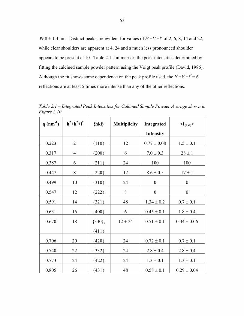
LIST OF TABLES
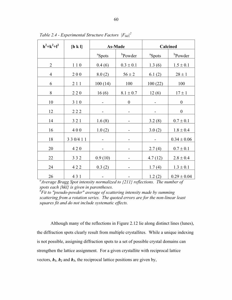
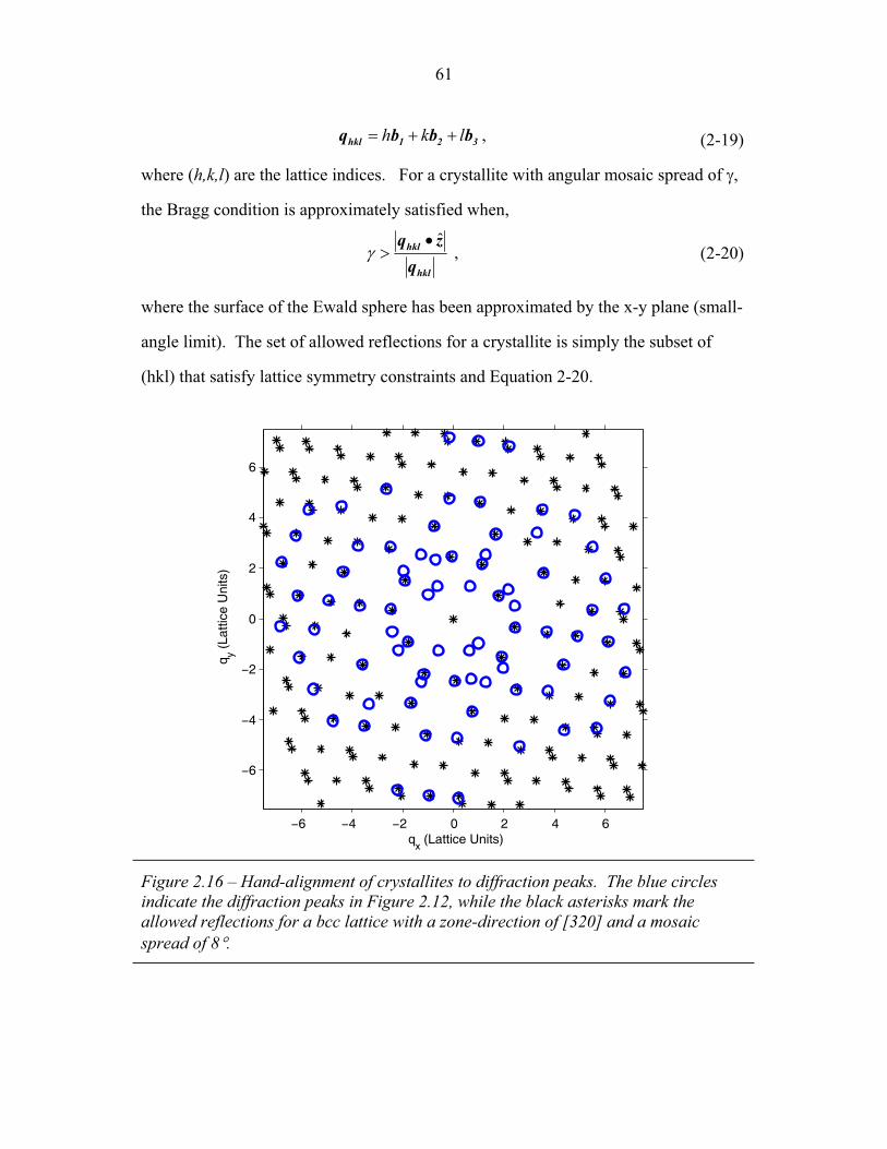
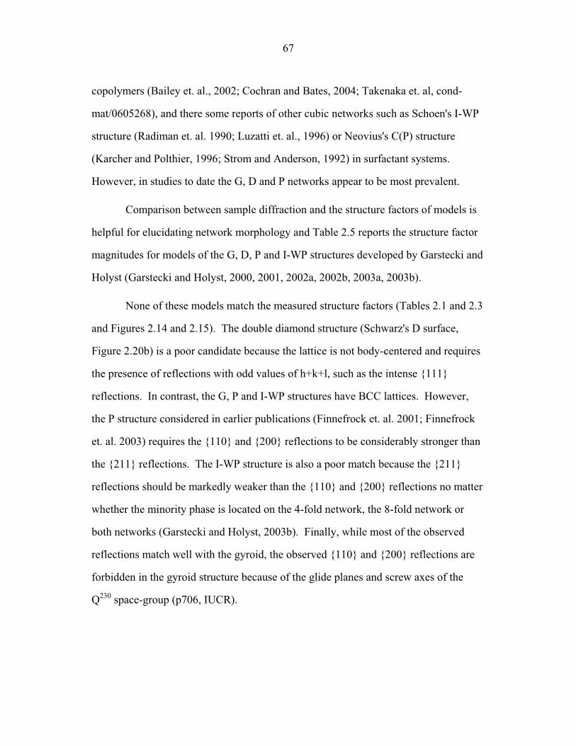
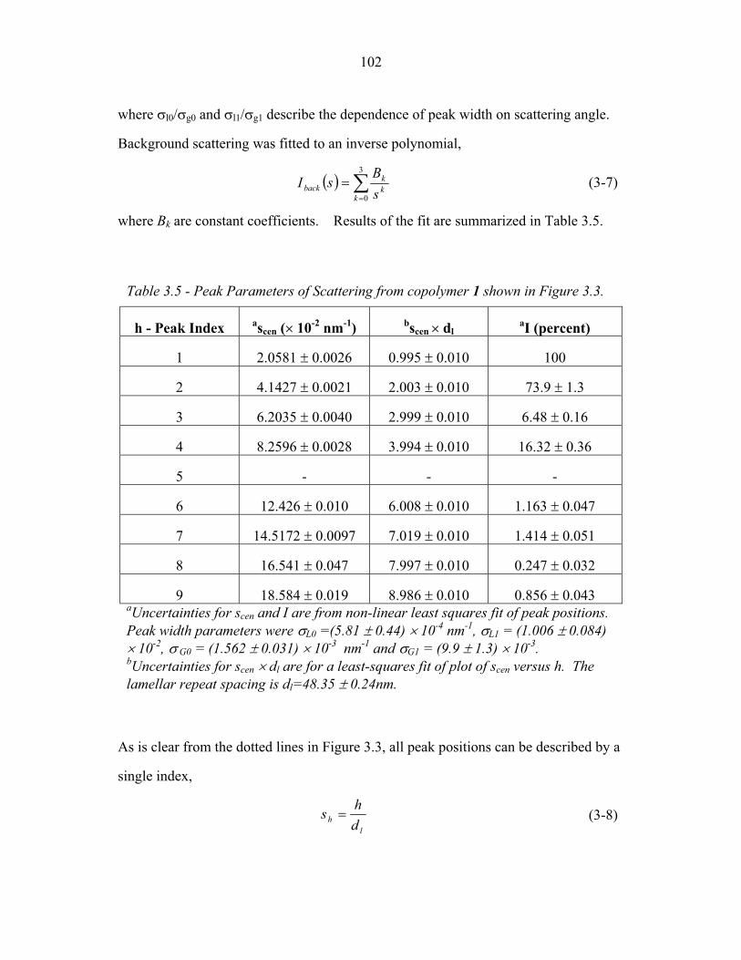
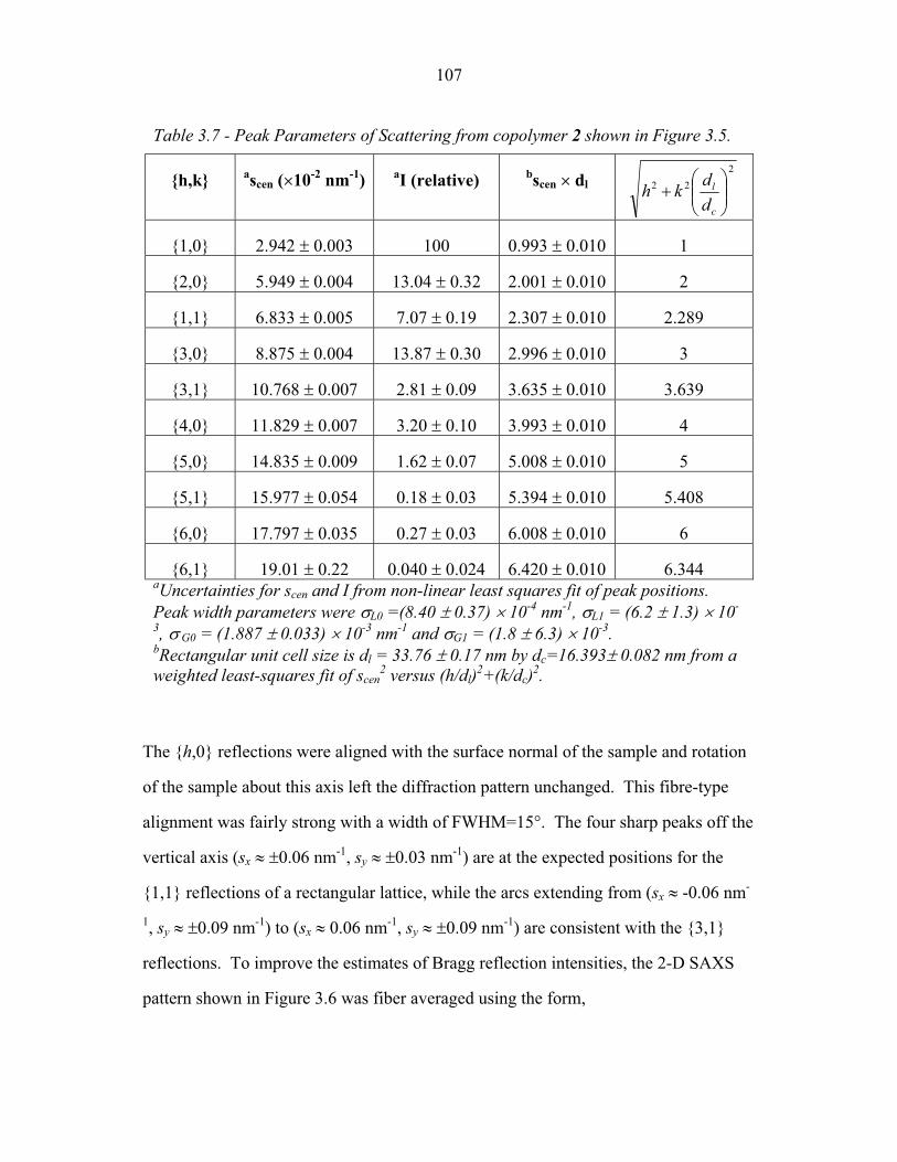
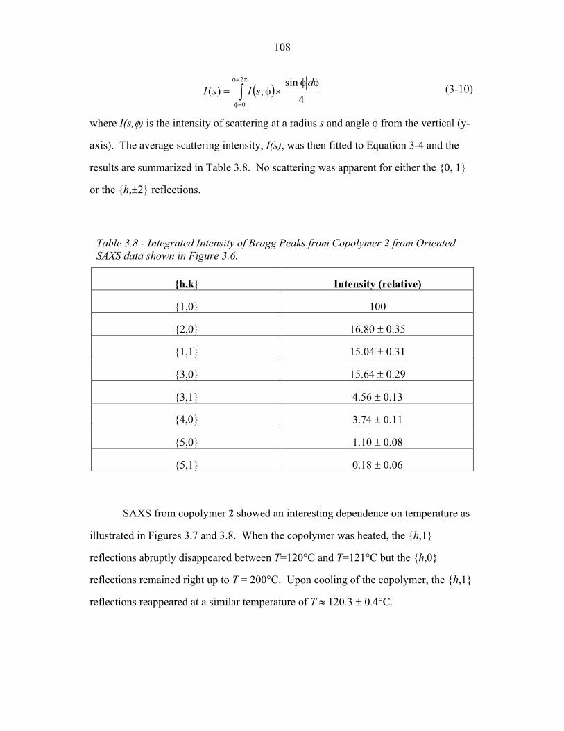
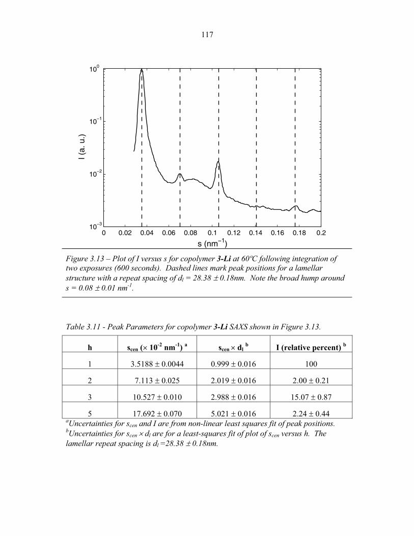
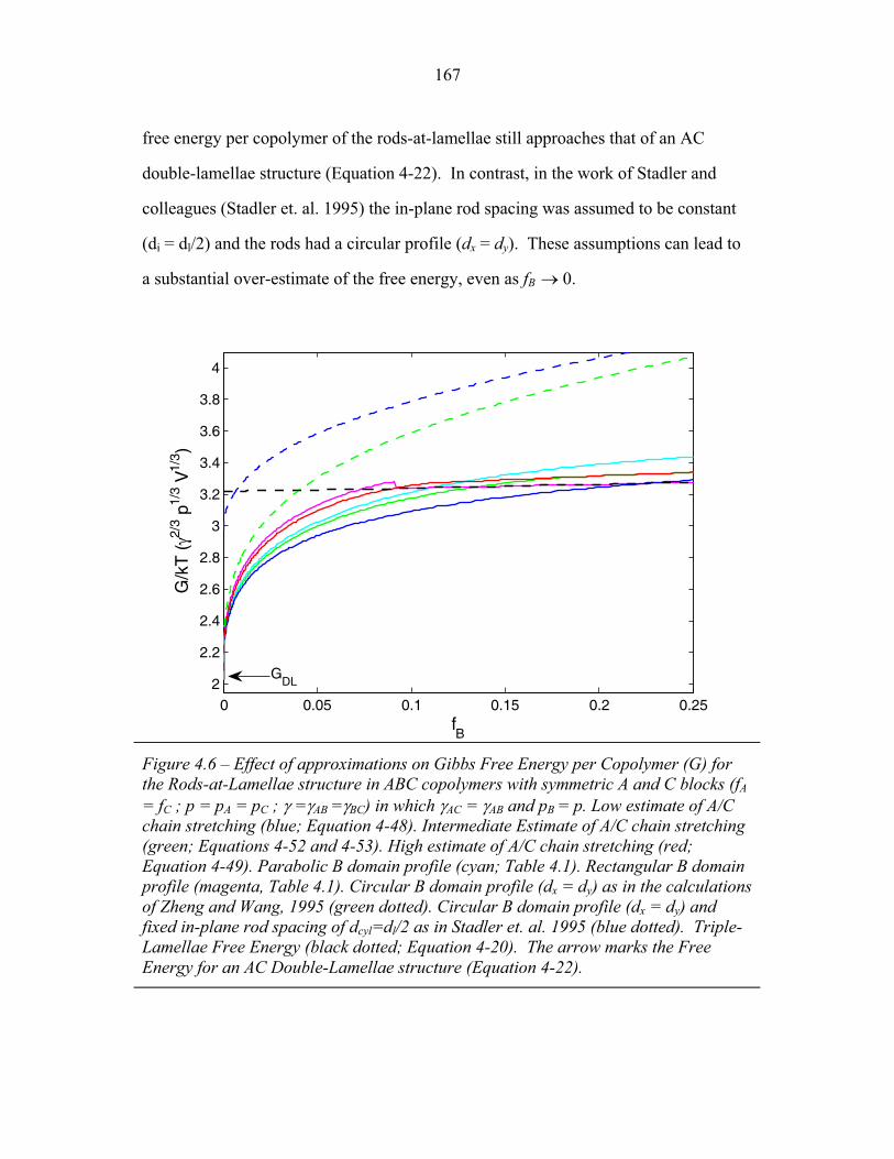
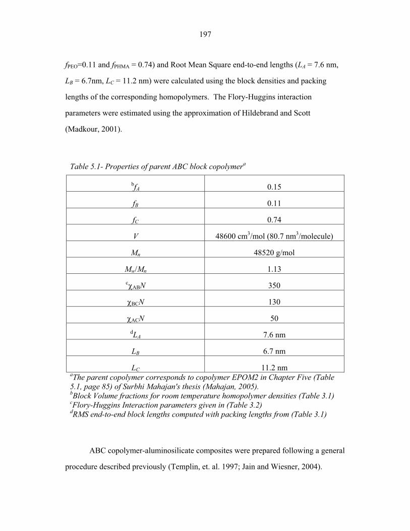
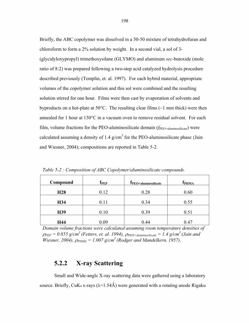
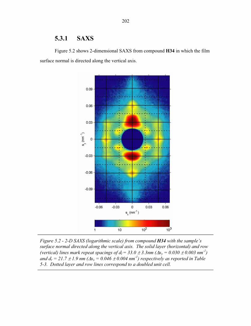
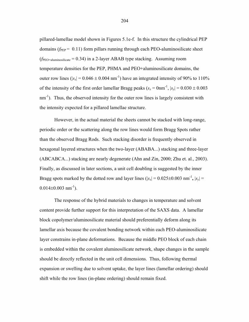
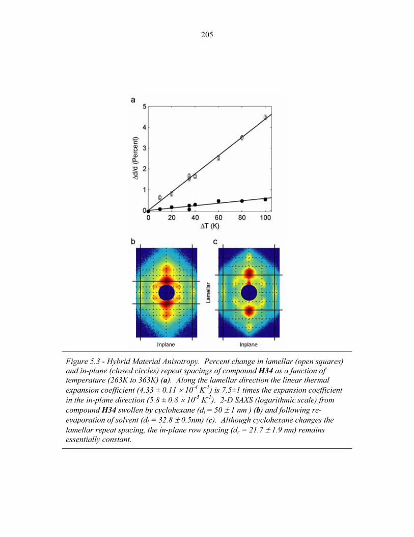
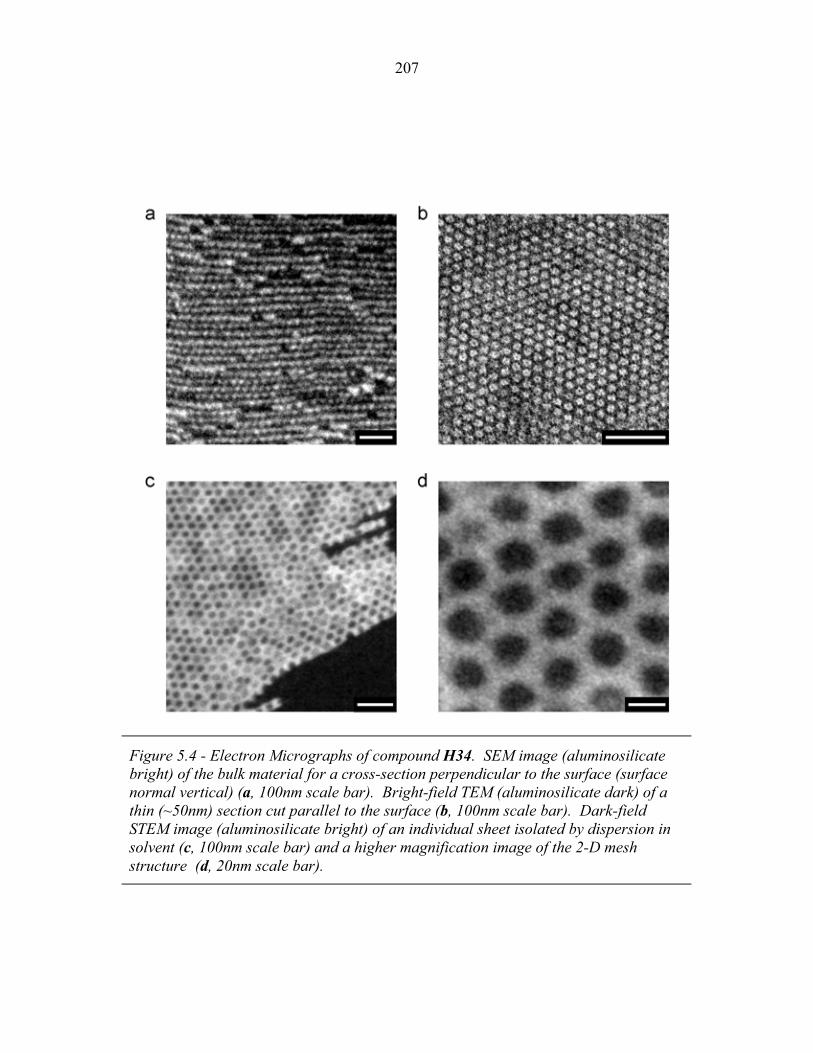
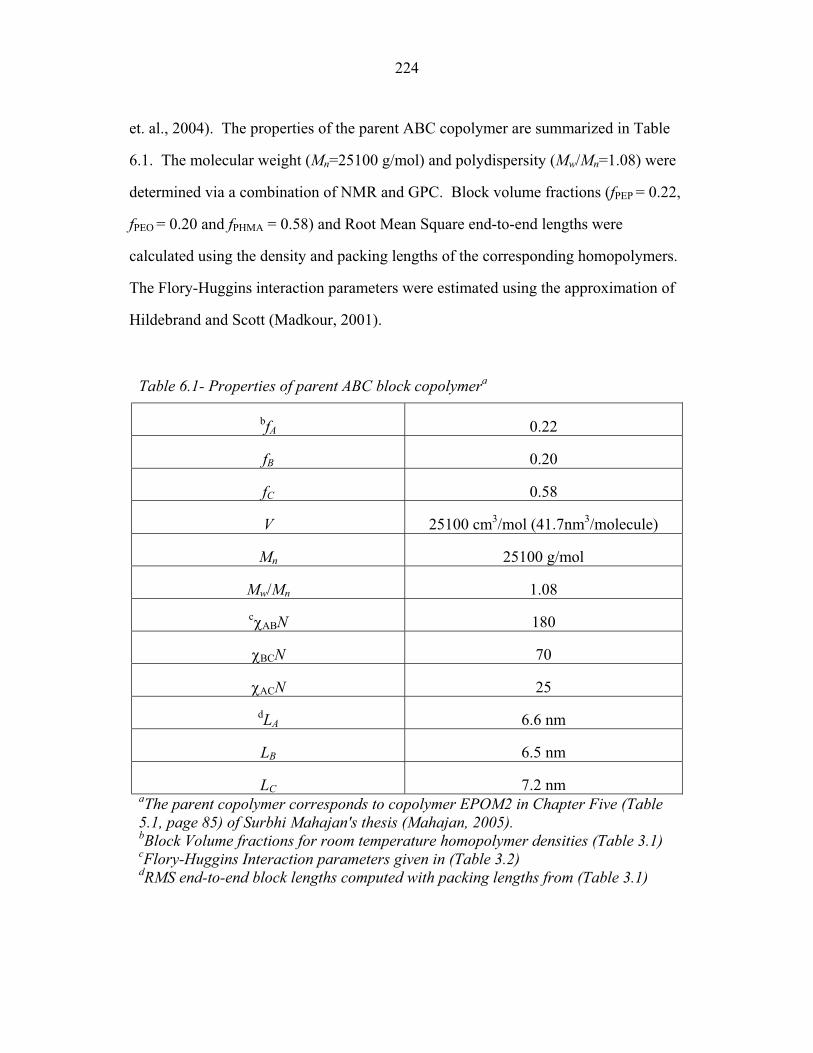
2.1 Integrated Peak Intensities from Calcined Material ............................. 53 2.2 Ellipse Parameters for Uncalcined Material ......................................... 54 2.3 Integrated Peak Intensities from As-Made Material ............................ 54 2.4 Experimental Structure Factors ............................................................ 60 2.5 Structure Factors for Bicontinuous Network Models .......................... 68 2.6 Projected Unit Cell Parameters from TEM Images ............................. 85 3.1 Molecular Properties of PEP, PEO and PHMA ................................... 94 3.2 Interaction Parameters of PEP, PEO and PHMA ................................. 95 3.3 Composition of Copolymers 1, 2 and 3 ................................................ 96 3.4 Composition of Copolymers 4 and 5 .................................................... 97 3.5 Structure Factors for Copolymer 1 ....................................................... 102 3.6 Structure Factors for Copolymer 1-Li .................................................. 104 3.7 Structure Factors for Copolymer 2 ....................................................... 107 3.8 Structure Factors for Copolymer 2 from 2-D SAXS ............................ 108 3.9 Structure Factors for Copolymer 2-Li .................................................. 112 3.10 Structure Factors for Copolymer 3 ....................................................... 115 3.11 Structure Factors for Copolymer 3-Li .................................................. 117 3.12 Triple-Lamellae Slab Model Parameters .............................................. 119 3.13 Experimental and Model Structure Factors for Copolymer 1 ............... 120 3.14 Experimental and Model Structure Factors for Copolymer 2 ............... 125 3.15 Experimental and Model Structure Factors for Copolymer 3 ...............130 3.16 WAXS Scattering ..................................................................................137 4.1 Rods-at-Lamellae parameterization ...................................................... 159 4.2 Balls-at-Lamellae parameterization ...................................................... 170 4.3 Free Energy of Copolymers 1, 2 and 3 in the SSL ............................... 192 5.1 Molecular Properties of Parent ABC Copolymer ................................. 197 5.2 Composition of ABC Copolymer/aluminosilicate hybrids ................... 198 5.3 Parameters from 2-D SAXS from Compound H34 .............................. 203 6.1 Molecular Properties of Parent ABC Copolymer ................................. 224
xiii
LIST OF ABBREVIATIONS 2-D two dimensional 3-D three dimensional AFM Atomic Force Microscopy �C degrees Celcius CCD Charge Coupled Detector cm centimeter CuK� K� X-rays from Copper (wavelength 0.154nm) EM Electron Microscopy FWHM Full Width Half Maximum GLYMO 3-(glycidyloxypropyl) trimethoxysilane HAADF High Angle Annular Dark Field (detector) IDL Interactive Data Language (software) K Kelvin (Temperature) kV kiloVolt Li-triflate Lithium trifluoromethanesulfonate log Natural Logarithm mA milliAmpere mg milligram �L microliter mm millimeter nm nanometer Pa Pascals PB poly(butadiene) PEELS Parallel Electron Energy Loss Spectroscopy PEO poly(ethylene oxide) PEP poly(ethylene-alt-propylene) PEP-b-PEO-b-PHMA poly(ethylene-alt-propylene-block-ethylene oxide-block-n-
hexyl methacrylate) PHMA poly(n-hexyl methacrylate) PMMA poly(methyl methacrylate) PI poly(isoprene) PI-b-PEO poly(isoprene-block-ethylene oxide) PS poly(styrene) SAXS Small Angle X-ray Scattering SCMFT Self Consistent Mean Field Theory S/cm Siemens per centimeter SEM Scanning Electron Microscopy SIRT Simultaneous Iterative Reconstruction Technique SSL Strong Segregation Limit STEM Scanning Transmission Electron Microscopy TEM Transmission Electron Microscopy �m micro-meter WAXS Wide Angle X-ray Scattering WSL Weak Segregation Limit
xiv
LIST OF SYMBOLS
a1, a2, a3 Real Space Lattice Vectors (Ch. 1, 2, 3, 6) Aball(�) Ratio of Surface Area to In-Plane Area for a Ball-Shaped Domain with
aspect ratio � (height/width). (Ch. 4) Acyl(sx, sy) Fourier transform of a rod in rods-at-lamellae structure (Ch. 3) Aij Area per unit cell of domain interfaces between blocks i and j. (Ch. 4) Aj
m Fourier amplitude describing elastic distortion of material (Ch. 2) Ap 2�3 matrix of a1, a2 and a3 projected into the x-y plane (Ch. 2) Aperf(�,�a) Ratio of Surface Area to In-Plane Area for a perforation in a lamellae
with aspect ratio � and in-plane area fraction �a (Ch. 4) Aring(�1,�2) Ratio of Surface Area to In-Plane Area for a toroidal domain with
aspect ratio �1 and ratio of toroidal to axial radii of �2. (Ch. 4) Arod(�) Ratio of Surface Area to In-Plane Area for a Rod-Shaped Domain with
aspect ratio � (height/width). (Ch. 4) Asph(sx,syz) Fourier transform of a ball in the balls-at-lamellae structure (Ch. 3) u(qj) Fourier Amplitude for Wave-Vector qj �j Rotation axis for crystallite (Ch. 2) b1, b2, b3 Reciprocal Space Lattice Vectors (Ch. 1, 2) B Intensity of background scattering around a Bragg Peak (Ch. 2) Bk Coefficients describing background scattering in powder pattern (Ch. 3) Bjk 3�3 matrix of reciprocal lattice vectors b1, b2 and b3 (Ch. 2) C Constant coefficient (Ch. 1). Cint Coefficient describing the Interfacial Energy per copolymer. (Ch. 4) Cstretch Coefficient describing the Stretching Energy per copolymer. (Ch. 4) ij Flory-Huggins Segment-Segment Interaction Parameter for Species X
and Y (dimensionless; Ch. 1) d Characteristic size of block copolymer structure generally taken to be
one of the lattice constants. (Ch. 4) d Cubic unit cell size (Ch. 2) dA Thickness of A domain (Ch. 1) dAC Diameter of the cylindrical AC interface in the rings-at-lamellae
structure (Ch. 4) dbox B-domain height when approximated by a box-shaped profile (Ch. 4) dB Average thickness of B-domain (Ch. 1, 4) dBB PHMA Backbone-Backbone Repeat Spacing (Ch. 3, 5 and 6) dc Distance between rods in the rods-at-lamellae structure (Ch. 3) dCC Side chain-side chain repeat spacing (Ch. 3, 5 and 6) dcyl Diameter of cylinders in the AB or ABA cylinder phase and rings-at-
cylinder structure. (Ch. 4) di In-plane spacing between domains (Ch. 4) dip Spacing Between Concertinas in plane (Ch. 6) dl Lamellar repeat spacing (Ch. 2, 3 and 4)
xv
dr In-Plane Row Spacing (Ch. 5) ds Distance between adjacent balls at the AC interface in the balls-at-
lamellae structures (Ch. 3) dSOL Sol-Sol particle repeat spacing (Ch. 6) dw Concertina Wiggle Period (Ch. 6) dx Height of B-domains (Ch. 3, 4) dy In-plane width of B domains (Ch. 3, 4) �i Hildebrand Solubility Parameter (Ch. 1, 3, 4, 5 and 6 ) �ij Kronecker Delta Matrix (Ch. 2) ejk(xl) Strain field at point Xj(xk) (Ch. 2) em
jk Fourier amplitudes of strain field (Ch. 2) � Ellipse eccentricity (Ch. 2) � Aspect ratio of rod, ball or perforation (Ch. 4) � Fractional Contraction (Ch. 6) �jkl Anti-symmetric tensor (Ch. 2) E(x) Complete Elliptic Integral of Second Kind (Ch. 4) fX Volume Fraction of Block/Phase X (Ch. 1-6) Fhkl Fourier Coefficient for reciprocal lattice vector (hkl) (Ch. 1) Fu(qj)/Fc(qj) Fourier amplitude for wave vector qj in the uncompressed/compressed
structure (Ch. 2) Fh
TL Fourier coefficient of the slab model of the triple-lamellae structure for the h-th harmonic (Ch. 3)
FhDL Fourier coefficient of the slab model of the double-lamellae structure
for the h-th harmonic (Ch. 3) Fhk
rods Fourier coefficient for (h,k) reciprocal lattice vector in the rods-at-lamellae structure (Ch. 3)
Fhklballs Fourier coefficient for (h,k,l) reciprocal lattice vector in the balls-at-
lamellae structure (Ch. 3) �� Sample Rotation angle (Ch. 2) �� � Angle at which concertina strands cross (Ch. 6) �a Fraction of plane of AC interface occupied by B-domains (Ch. 4) �A Fraction of B-domain on A side of AC interface (Ch. 3, 4) �C Fraction of B-domain on C side of AC interface (Ch. 3, 4) �cyl(x,y) Fourier transform for a half-cylinder (Ch. 3) �i Ratio of B-domain in-plane spacing to lamellar repeat spacing. (Ch. 4) �n Azimuth of film normal in the un-rotated sample (Ch. 2) �sph(x, y) Fourier transform of a half-ellipsoid (Ch. 3) G Gibbs free energy per copolymer (Ch. 4) Gint Component of Gibbs free energy per copolymer from enthalpy of
mixing at domain interfaces (Ch. 4). Gstretch Component of Gibbs free energy per copolymer from stretching of
chains into domain interiors. (Ch. 4) G[�i] Change in Free Energy per copolymer relative to disordered state.
�ij �ij �kBT is the Enthalpy of mixing per unit area (surface tension) between blocks i and j (Ch. 3, 4)
(h,k,l) Reciprocal lattice vector (Ch. 1) {h,k,l} Set of symmetry-related reciprocal lattice vectors (Ch. 1) h(y) Function describing B-domain interface shape (Ch. 4) Hn,cyl Integrated moments of domain profile (Ch. 4) Hsegment(x) Enthalpy of Mixing per segment at point x (Ch. 1) H[�i] Average mixing enthalpy per copolymer (Ch. 1) ��C Mean squared path length of block A/C relative to mean squared
end-to-end length of block A/C in triple-lamellar structure with same lattice size. (Ch. 4)
�B Mean squared path length of chains in the block B relative to a lamellar B domain of the same average thickness. (Ch. 4)
I, I(s), I(sx,sy) Scattering intensity per steradian (Ch. 1, 2, 3, 5 and 6) <I{hkl}> Average intensity of Bragg Reflections {hkl} (Ch. 2) IAVG(s) Average Scattering intensity per steradian (Ch. 2) Iback(s) Intensity of background scattering in powder pattern (Ch. 3) I0 Integrated intensity of Bragg spot (Ch. 2) Ij Integrated intensity of scattering peak in powder pattern (Ch. 3) � Rotation angle (Ch. 2) �AC Coefficient relating area of AC interface to area of AB/BC interfaces in
triple-lamellar structure. (Ch. 4) �AB Ratio of AB interfacial area to area of AB interface projected into the
plane of the AC interface. (Ch. 4) �BC Ratio of BC interfacial area to area of BC interface projected into the
plane of the AC interface. (Ch. 4) kB Boltzmann's Constant (Ch. 1, 4) kincident Wave-vector of the incident X-ray (Ch. 1) kscattered Wave-vector of the scattered X-ray (Ch. 1) L Distance between sample and detector in SAXS beam line (Ch. 1) LX Root mean squared end-to-end length of a polymer chain of type X in a
homopolymer melt (Ch.1, 3, 4, 5 and 6) � X-ray Wavelength (Ch. 1) �(xl) Second Lame elastic coefficient at point xl (Ch. 2) �m Fourier coefficients of second Lame elastic coefficient (Ch. 2) Mjk 3*3 Transformation Matrix describing sample compression (Ch. 2) Mi Molecular Weight of a copolymer (Ch. 1) Mn Number Average Molecular Weight (Ch.1-6) Mw Weight Average Molecular Weight (Ch. 1-6) MX Molecular Weight of X (Ch. 1) �(xl) First Lame elastic coefficient at point xl. (Ch. 2) �m Fourier coefficients of first Lame elastic coefficient (Ch. 2) N Average Number of segments in a copolymer. (Ch. 1-6) NX Average Number of segments of type X in copolymer (Ch. 1) ni Number of molecules (Ch. 1)
xvii
nj Sample surface normal (Ch. 2) pj Packing Length of Polymer j (Fetters, et. al. 1999; Ch 1, 3, 4, 5 and 6) q Scattering wave vector (q=|q| = 4��sin(�)/�; q = 2��� s ; Ch. 1, 2) q Magnitude of scattering wave vector q (Ch. 1, 2) qx, qy Components of scattering wave vector (Ch. 2) qj
u Position in reciprocal space prior to film compression (Ch. 2) qk
c Position of same point following film compression (Ch. 2) q0 Magnitude of scattering wave vector before film compression (Ch. 2) qr Radius of scattering ellipse at angle � on detector (Ch. 2) qru Scattering ellipse radius at angle �u in uncompressed structure (Ch. 2) qmin, qmax Minor and Minor Radii of scattering ellipse (Ch. 2) �q Average radial width of Bragg scattering peak (Ch. 2) � Bragg Scattering Angle (2� is angle between incident and scattered X-
ray; Ch. 1, 2, 3, 5 and 6) �� Angle on detector from rotation axis (Ch. 2) �0 Angular position of Bragg Spot on detector (Ch. 2) �bc Angle between the two in-plane lattice vectors in the balls-at-lamellae
structure (Ch. 3) �e Angle between the scattering ellipse major axis and the y-axis (Ch. 2) �n Altitude of film normal in the un-rotated sample (Ch. 2) �u Angle on detector from rotation axis in uncompressed structure (Ch. 2) �w Angular width of Bragg scattering peak (Ch. 2) �� Average angular width of Bragg scattering peak (Ch. 2) �c(xk) Electron density at point xk in the compressed structure (Ch. 2) �e(x) Electron density at point x. (Ch. 1) �i(x) Fraction of segments of type X at point x (dimensionless; Ch. 1) �u(xk) Electron density at point xk in the uncompressed structure (Ch. 2) �X Density of homopolymer X (g/cm3 ; Ch. 1, 2, 3, 5 and 6) r0 Radius of Bragg Spot on detector (Ch. 2) rAB Radius of the inner half-toroid in the rings-at-cylinders structure (Ch. 4) rBC Radius of the outer half-toroid in the rings-at-cylinders structure (Ch. 4) rj(u) Function describing the path followed by the backbone of a continuous
Gaussian chain (u is the fractional distance along the backbone; 0 � u � 1; ends of polymer chain at rj(0) and rj(1)). (Ch. 1, 4)
rw Radial width of Bragg scattering peak (Ch. 2) Rj Average root mean square path length of block j. (Ch. 4) Rkl Unitary 3�3 rotation matrix (Ch. 2) s Scattering vector (s=|s| = 2sin(�)/� = q / (2�)) (Ch. 1, 3, 5 and 6). s Magnitude of scattering vector s (Ch.1, 3, 5 and 6) scen,j Center of j-th scattering peak in a powder pattern (Ch. 3) smin Magnitude of minimum accessible scattering vector (Ch. 1) sx, sy, sz Component of scattering vector (e.g. sx = qx/(2�)) (Ch. 3, 5 and 6) Sjk(xl) Stress field at point xl (Ch. 2) Sm
jk Fourier coefficients of stress field (Ch. 2) S(sy) In-plane rod-rod correlation function (Ch. 3)
xviii
Ssph(syz) In-plane ball-ball correlation function (Ch. 3) S[�i] Change in Entropy per copolymer relative to disordered state. (Ch. 1) �0 Root Mean Square displacement amplitude of the distance between
nearest neighbors (Ch. 3) �g Gaussian component of Voigt peak shape (Ch. 3) �l Lorentzian component of Voigt peak shape (Ch. 3) t Thickness of contracted film relative to uncontracted film (Ch. 2) tij Thickness of interface between polymers i and j (Ch. 3) T Temperature (Ch. 1, 4) Tg Polymer Glass Transition Temperature (Ch. 1) Tm Polymer Crystallization Temperature (Ch. 1) u Fractional distance along a polymer backbone (Ch. 1, 4) Ue Average elastic energy per unit volume (Ch. 2) V Molecular volume of the copolymer. (Ch. 1) Vcell Volume of the unit cell. (Ch. 2, 4) Vchain Volume of a polymer chain. (Ch. 1, 4) Vref Reference volume taken to be the effective "segment" volume (Ch. 1) Vsample Volume of the sample (Ch. 1) VX Molecular Volume of block X (Ch. 1) V(x,�l,�g) Voigt Function (Ch. 3) wi(x) Mean-field Potential for segments of type i at position x (Ch. 1) wj Relative width of the j-th slab in the slab model of the triple-lamellae
structure. (Ch. 3) [x,y,z] Direction in real space lattice (Ch. 1) <x,y,z> Set of symmetry-related directions in real space lattice (Ch. 1) xk
u Position of a point in sample before compression (Ch. 2) xj
c Position of a point in sample after compression (Ch. 2) xe,ye Coordinates of direct beam on detector (Ch. 2) Xj(xk) Position a point xk is mapped to following elastic distortion (Ch. 2) xj Relative position of center of j-th slab in the slab model of the triple-
lamellae structure (Ch. 3) y1 Relative offset between the first and second rods along the y-axis for
the rods-at-lamellae structure (Ch. 3) y1, z1 Relative offset between the balls at the two AC interfaces along the two
in-plane crystal axes in balls-at-lamellae structure (Ch. 3) z Chain stretching distance. For each point in a domain, z is the distance
chains with ends at that point must stretch to reach the domain interface (Milner et. al. 1988; Ball et. al. 1991). (Ch. 4)
1
Chapter One – Introduction
In a block copolymer, two or more chemically distinct polymer chains (blocks)
are joined by covalent bonds to form a single macromolecule (Hamley, 1998, Ch1, p1;
Figure 1.1). The covalent linkages between these individual blocks prevent
macroscopic phase separation even when the polymer blocks are thermodynamically
incompatible. Instead, the individual blocks can microphase separate to form domains
with sizes comparable to the dimensions of the individual polymer chains (1-100nm)
as is illustrated in Figure 1.2. Because individual blocks can be selected to confer
distinct chemical or physical properties, block copolymers have found extensive
industrial applications including use as structural plastics, blend stabilizers, emulsifiers
and contact sensitive adhesives (Ruzette and Leibler, 2005).
Many applications rely primarily upon the ability of block copolymers to
suppress macroscopic phase separation (Lodge, 2003). Increasingly there is interest in
also harnessing the ability of block copolymers to form numerous nanometer-scale
structures. For example, block copolymers can act as templates directing the assembly
of inorganic precursors into periodic structures (Templin, et. al. 1997; Bockstaller, et.
al. 2005). These block copolymer/inorganic composite materials may be of use for
selective membranes, catalysts, porous electrodes, low dielectric insulators and optical
materials (Bockstaller et. al., 2005). However, the structure directing capacity of
block copolymers is only now being explored.
This thesis reports the structural characterization of block copolymer and
copolymer/inorganic materials prepared in the laboratory of Professor Uli Wiesner in
the Department of Material Science at Cornell University. The results contribute to
the understanding of structure formation in multi-domain and multi-component
2
polymeric systems. In particular, the structural effects of a third, chemically distinct
block was studied for a set of ABC block copolymers and a new, four-layer woodpile
structure was identified in an ABC triblock copolymer/aluminosilicate material.
The remaining sections of this chapter provide an overview of block
copolymer physics and the use of block copolymers as structure-directing agents.
There are several good introductions to the physics of block copolymers (Hamley,
1998; Matsen, 2002; Grason, 2006) and the discussion in this chapter closely follows
Bates and Fredrickson's article in "Physics Today" (Bates and Fredrickson, 1999).
Section 1.1 describes the molecular structure of block copolymers and
introduces the notation used to describe their physical properties. The thermodynamic
properties of polymer melts and solutions are summarized in Section 1.2. The entropy
of each copolymer chain is described in terms of the continuous Gaussian chain model
while the enthalpy of mixing between the thermodynamically incompatible blocks is
described using the Flory-Huggins segment-segment interaction parameter (ij).
Microphase separation of individual blocks into nanometer-sized domains reduces the
mixing enthalpy per copolymer but also lowers the entropy per copolymer. Section
1.3 describes the general order-disorder transition resulting from this trade-off
between enthalpy and entropy. The relative strength of interactions between the
blocks (ij) then determines whether the copolymer blocks are mixed, weakly
segregated (WSL) or strongly segregated (SSL). Section 1.3 also summarizes existing
analytic and computational descriptions of block copolymer structures in the limits of
weak, intermediate and strong segregation.
After many years of theoretical and experimental work, the phase behavior of
AB diblock copolymers is relatively well understood (Matsen and Bates, 1997).
Section 1.4 summarize this phase behavior and uses the preferred interfacial curvature
3
between domains to provide a qualitative explanation for the known AB diblock
structures (Matsen, 2002; Grason, 2006). Compared to AB diblock copolymers, the
phase behavior of ABC triblock copolymers is far more complicated and not nearly as
well understood (Bates and Fredrickson, 1999). Progress in this area is summarized in
Section 1.5 along with a discussion of current experimental challenges in this area.
The use of organic molecules to the direct the assembly of inorganic precursors
has been the subject of considerable research and is reviewed in a number of
In the work described in this thesis, block copolymer and copolymer/inorganic
materials were characterized using a variety of experimental techniques such as
Transmission Electron Microscopy (TEM) and Small Angle X-ray Scattering (SAXS).
Although the SAXS technique is very similar to conventional X-ray scattering, an
overview of SAXS is provided in Section 1.7 to complement introductory texts upon
this subject (Als-Nielsen and McMorrow, 2001; Glatter and Kratky, 1982).
Finally, Section 1.8 provides an overview of the topics discussed in the
remaining chapters.
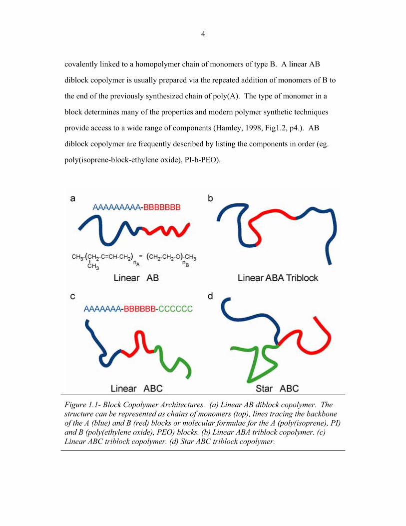
1.1 Molecular Structure As illustrated in Figure 1.1, the molecular structure of a block copolymer
depends upon the number and type of blocks and the manner in which the blocks are
connected together. The simplest architecture is the linear AB diblock copolymer
shown in Figure 1.1a, in which a homopolymer chain of monomers of type A is
4
covalently linked to a homopolymer chain of monomers of type B. A linear AB
diblock copolymer is usually prepared via the repeated addition of monomers of B to
the end of the previously synthesized chain of poly(A). The type of monomer in a
block determines many of the properties and modern polymer synthetic techniques
provide access to a wide range of components (Hamley, 1998, Fig1.2, p4.). AB
diblock copolymer are frequently described by listing the components in order (eg.
poly(isoprene-block-ethylene oxide), PI-b-PEO).
Figure 1.1- Block Copolymer Architectures. (a) Linear AB diblock copolymer. The structure can be represented as chains of monomers (top), lines tracing the backbone of the A (blue) and B (red) blocks or molecular formulae for the A (poly(isoprene), PI) and B (poly(ethylene oxide), PEO) blocks. (b) Linear ABA triblock copolymer. (c) Linear ABC triblock copolymer. (d) Star ABC triblock copolymer.
5
More complicated molecular structures can be achieved by the addition of
extra blocks. For example, the poly(styrene-block-butadiene-block-styrene) (PS-b-
PB-b-PS) copolymers widely used in the footwear industry correspond to the linear
ABA triblock copolymer architecture shown in Figure 1.1b. Alternatively, the linear
ABC triblock copolymer structure shown in Figure 1.1c can be formed by the addition
of a third type of monomer (C). Finally, alternative synthetic techniques can be used
to form branched architectures such as the star ABC triblock copolymer morphology
shown in Figure 1.1d. In the work described here, only block copolymers with AB
diblock or linear ABC triblock architectures are considered.
Within the field of polymer science, the average size of a block copolymer is
frequently described in terms of the number average molecular weight (Mn), and
weight average molecular weight (Mw) defined as,
� �
��
�� �
��
iii
iiii
w
ii
iii
n Mn
MMnM
n
MnM , , (1.1)
where ni is the number of molecules with molecular weight Mi. The polydispersity
index is defined as the ratio of Mw/Mn and is equal to 1 for a monodisperse system.
Actual block copolymers can have quite low polydispersity indices (Mw/Mn < 1.1)
thanks to synthetic approaches such as living anionic polymerization (Bates and
Fredrickson, 2003). Both theory (Sides and Fredrickson, 2004; Cooke and Shi; 2006)
and (Lynd and Hillmyer, 2005; Noro et. al., 2005) experiment suggest this level of
polydispersity has only a small effect on the phase behavior of AB diblock
copolymers.
An effective volume for the block copolymer, V, can be defined as,
...��
��
�B
B
A
A MMV , (1.2)
6
where MX is the number average molecular weight of block X and �X is the density of
the corresponding homopolymer. The size of individual blocks can be expressed in
terms of their number average molecular weight (MX) or molecular weight fractions.
However, it is again convenient to describe their size in terms of effective block
volume fractions,
VM
VV
fX
XXX �
�� , (1.3)
where VX is the volume a homopolymer corresponding to polymer block X.
Because the monomers in each block can differ substantially in size, it is more
convenient to think of the chains in terms of segments, each of volume Vref (commonly
taken to be the average monomer volume). The average number of segments per
copolymer, N, can then be defined as,
refVVN � , (1.4)
while the average number of segments in block X is given by,
NfVVN X
ref
XX �� . (1.5)
1.2 Polymer Thermodynamics The physics of polymeric and block copolymer systems is described in a
number of introductory texts and review articles (Lifshitz et. al., 1979; Young, 1983;
Bates and Fredrickson, 1990; Hamley, 1998; Matsen 2002). The interactions between
monomers, temperature and presence of solvent all have significant effects upon the
physical state of a polymeric system. For example, at room temperature the chains in
polyethylene (widely used in plastic bags) are organized into a semi-crystalline
structure while the chains in polystyrene (used in drinking cups and as a packing
foam) are trapped in a glassy, amorphous state. In both the crystalline and glassy
7
states, the monomers are frozen in place and the system behaves as a solid (Hamley,
1998).
When polyethylene is heated above its melting temperature (Tm) or polystyrene
is heated above its glass transition temperature (Tg), the monomers can move past each
other and develop local, liquid-type ordering. In this state, commonly referred to as a
melt, each polymer backbone can explore a vast range of conformations and also
move throughout the system. Because monomers cannot freely move in the glassy or
crystalline states, microphase separation in block copolymers must be studied above
the glass (Tg) or crystallization (Tm) temperatures of the individual polymer blocks.
Solvents can also dramatically transform the state of polymeric system. For example,
at room temperature a solid polystyrene cup can be rapidly dissolved in acetone
(commonly used in nail polish remover) to form a goopy, fluid mess and the
polystyrene does not return to the solid, glassy state until most of the solvent has
evaporated. Solvents are very useful for increasing the mobility of polymer chains
and can be used to mix polymers that would otherwise be solid at a particular
temperature.
The thermodynamic behavior of polymer melts and polymer solutions was first
described by Huggins (Huggins, 1941) and Flory (Flory, 1942). In the Flory-Huggins
model, the monomers of the polymer and individual solvent molecules are described
in terms of units or segments (volume Vref) that are assumed to occupy space with a
constant number of segments per unit volume. The local concentration of monomers
(or solvent molecules) of type X, can then be described in terms of the average
fraction of segments, �X(x), of type X residing at a point, x. Interactions between
segments are assumed to be short-ranged and to depend only upon the local
concentration of the different types of segment. In contrast, the entropy of each
8
polymer is a non-local quantity because it depends upon the number of allowable
conformations for the entire polymer backbone. Despite its simplicity, this mean-field
approach of Huggins and Flory works remarkably well for a wide range of polymeric
systems (Young, 1983; Hamley, 1998). The success of the Flory-Huggins model
depends in part upon each polymer chain having an enormous number of degrees of
freedom (>> 100). Because the enthalpy/entropy of each chain depends upon the sum
of interactions/conformations along the chain, the significance of fluctuations at
individual segments of the chain are considerably reduced.
The configurational entropy of a polymer chain depends upon the allowed
paths of the polymer backbone. In a homogeneous melt, attractive and repulsive
interactions between monomers average out over short distances so the path of the
polymer backbone approximates a random walk (Flory, 1949). Thus, for a sufficiently
long chain the unperturbed root mean squared end-to-end length, LX, is given by,
X
XX p
VL � , (1.6)
where VX is chain volume and px is defined as the monomer packing length (Fetters,
et. al. 1999). Fetters and colleagues (Fetters, et. al. 1994 and 1999) have assembled
extensive tables of packing lengths for easy calculation of molecular scale, LX, for
different polymers.
In a spatially inhomogeneous melt, the variations in monomer density restrict
the allowed conformations of the polymer chains, decreasing their entropy. For block
copolymers, this loss in entropy is often approximated using the continuous flexible
Gaussian chain model (Matsen, 2002). In this model, the position of each point along
the polymer backbone is described by the continuous function, rX(u), where the
variable u is the fractional distance along the backbone (0 � u � 1) and the ends of the
chain are located at rX(0) and rX(1). Stretching a section of the chain reduces the
9
number of allowed conformations, decreasing entropy and increasing the Gibbs free
energy of the chain. For a given path of the backbone, rX(u), the stretching energy of
the chain is given by (Matsen, 2002),
� �� � � ���
�
!"
#$%���
1
0
2
Xstretch, 23 u
u
X
X
XBX du
duudr
VpTkurG , (1.7)
where kB is Boltzmann's constant and T is the temperature.
The mixing enthalpy per copolymer in the Flory-Huggins model is given by
the sum of mixing enthalpies for the each segment along the chain. In this model, the
segments surrounding each polymer segment act as a solvent for it and the interactions
between these segments are described in terms of the dimensionless Flory-Huggins
segment-segment interaction parameter, ij. Theoretically, ij is defined such that kBT
�ij is the increase in enthalpy when a segment of type i is inserted into a solution of
segments of type j (Lodge, 2003). This idealized definition is rarely achieved in
experimental measurements of ij, but the “experimentalist’s ij” is still a useful
descriptor of the interactions between different chemical species. The Flory-Huggins
interaction parameter can be roughly estimated using a semi-empirical relationship
first proposed by Hildebrand and Scott (Madkour, 2001),
� �Tk
V
B
jirefij
2��
&�� , (1.8)
where �i and �j are the Hildebrand solubility parameters for the two polymers. As is
evident from Equation 1.8, �i has units of (Energy/Volume)1/2 (e.g. J1/2m-3/2) and
values of these solubility parameters are tabulated for a wide range of monomer
species (Brandrup and Immergut, 1989). For most pairs of polymers the interaction
parameter, ij, is small and positive (ij = 0.001 to 0.1 typically; Semenov, 1985).
When the interactions between segments are weak and local, the presence of a
segment of type i at a point x does not have a large effect upon the local fraction of
10
segments of type j, �j(x), in the neighborhood of point, x. Assuming the interactions
are essentially pair-wise, the average mixing enthalpy per segment at point x is then
given by,
� � � � � ��'
�� ijj
jiijBTkH,
segment 21 xxx �� . (1.9)
Each block copolymer molecule has an average of N segments so the average mixing
enthalpy per copolymer is simply the sum over these segments given by,
� � � � � ��'
�� jiji
jiij
Bi
NTkH
;, 2 xxx ��
� (1.10)
where the average is taken over the volume of the system. Because the mixing
enthalpy per copolymer is proportional to the average number of segments per
copolymer (N), the product, ijN, is widely used to describe the thermodynamic
incompatibility of pairs of polymer blocks. Note that ijN does not dependent upon
the polymer segment volume, Vref, because ij depends linearly upon Vref while N is
inversely proportional to Vref. Even when the mixing enthalpy per segment is small
(ij < 1), the mixing enthalpy per copolymer can still be very significant (ijN >> 1)
because of the large number of segments in each copolymer (N ~ 102 to 106 typical).
Experimentally, the thermodynamic incompatibility between blocks i and j
(ijN) can be controlled in several different ways. During synthesis, chemical
modification of individual blocks (ij) and changes to average number of segments per
copolymer (N) have direct and obvious effects upon ijN. Following synthesis, the
value of ijN can still be manipulated through its dependence on temperature (T) and
solvent content. In general, the mixing enthalpy per monomer ( Hi) has a weak
dependence on temperature (T) and so ijN increases as temperature is lowered and
ijN decreases as temperature is increased (ij ( A/T+B; Bates and Fredrickson, 1990).
The effective value of ijN can also be reduced through the addition of good solvent
11
(one compatible with each type of monomer in the copolymer). Because a good
solvent mixes well with all blocks, the copolymer segment density is lowered along
with the total number of unfavorable interactions between different segments. Thus,
the relative incompatibility of blocks i and j (ijN) can be reduced by heating or the
addition of solvent while ijN is increased by cooling or the removal of solvent.
Finally, it should be noted that in addition to the chain entropy and mixing
enthalpy, other interactions are present in block copolymers. For example, long-range
electrostatics can be important in ionic polymers (ionomers) and long-range
interactions can also arise when the individual monomers have permanent dipole
moments (Sayar et. al., 2003). The effect of permanent dipole moments on phase
behavior has been modeled (Petschek and Wiefling, 1987; Halperin, 1990) but has not
yet been shown to play a significant role in most block copolymer systems (Sayar et.
al., 2003; Goldacker et. al., 1999).
1.3 Microphase Separation Within a block copolymer melt, micro-domains can reduce the unfavorable
enthalpy of mixing but they also reduce the entropy of the polymer chains. The
resulting structure depends upon the interplay between the enthalpy and entropy.
Different copolymer structures (including the disordered state) can be characterized by
the spatial dependence of the local volume fraction of each monomer species, �i(x).
Taking the isotropic state (�i(x) = fi) as a reference, the change in enthalpy per
copolymer is simply,
� � � � � �
� �� � � �� � .2
22
;,
;, ;,
�
� �
'
' '
&�&�
&�
jijixjjii
ij
jiji jijiji
ij
xjiij
B
i
ffN
ffNN
TkH
xx
xx
��
��
�
(1.11)
12
Clearly, the mixing enthalpy per copolymer can by lowered by density fluctuations
and for a diblock copolymer all density modulations lower the enthalpy relative to a
homogeneous state. The change in entropy per copolymer, S[�i], is also a unique
functional of the density distribution and is guaranteed to positive since the maximum
entropy corresponds to the homogenous state (�i(x) = fi). Thus, the free energy of a
structure relative to the homogenous state is given by,
� � � � � �
� �� � � �� � � � .2;, B
i
jijijjii
ij
B
ii
B
i
kSff
NTk
STHTk
G
���
���
�&�&�
& �
�' x
xx
(1.12)
Entropy favors more homogenous density distributions while the magnitude of the
interaction parameters (ijN) determines the relative benefits of density modulations.
As the equilibrium state corresponds to the global minimum of G[�i], order-disorder
or order-order transitions can be driven by changes in the interaction parameters
(ijN).
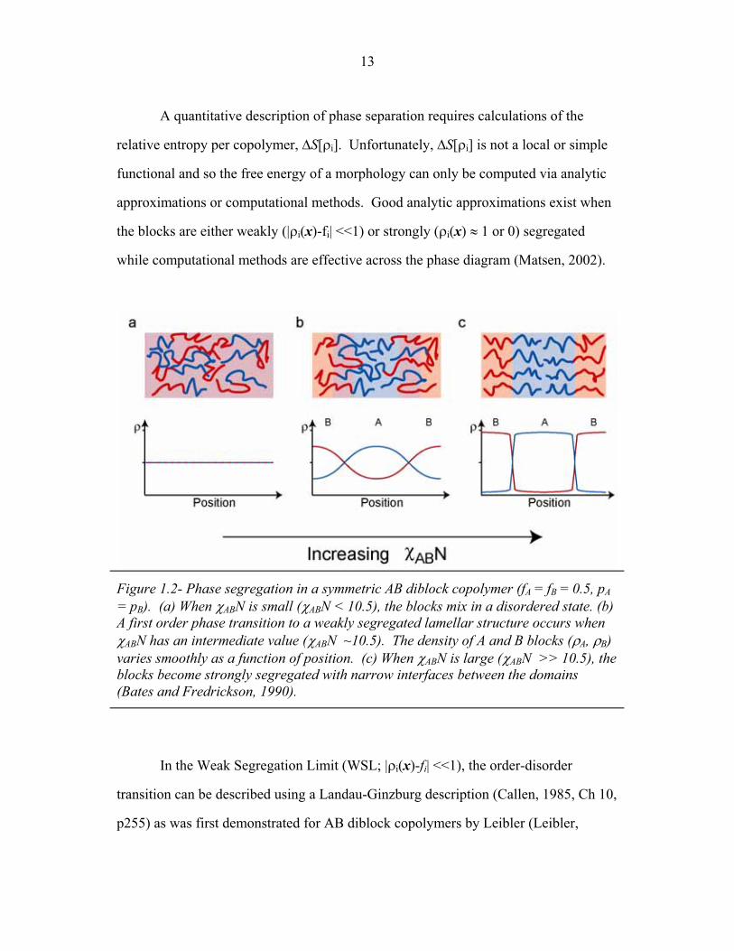
Figure 1.2 illustrates this process for a symmetric (fA = fB, pA = pB) AB diblock
copolymer. When ABN is small, enthalpy is less significant and the disordered state
has the lowest free energy. As the value of ABN increases, the enthalpy of the
disordered state becomes prohibitive and the system undergoes a first-order phase
transition into a weakly segregated lamellar structure (Figure 1.2b). For large values
of ABN, the blocks become strongly segregated and the blocks only mix in a narrow
region at the domain interfaces (Figure 1.2c). As noted in the previous section,
lowering the temperature increases ABN while heating or the addition of solvent
reduces ABN. Thus, temperature and solvent content can be used to switch between
the ordered and disordered states.
13
A quantitative description of phase separation requires calculations of the
relative entropy per copolymer, S[�i]. Unfortunately, S[�i] is not a local or simple
functional and so the free energy of a morphology can only be computed via analytic
approximations or computational methods. Good analytic approximations exist when
the blocks are either weakly (|�i(x)-fi| <<1) or strongly (�i(x) ( 1 or 0) segregated
while computational methods are effective across the phase diagram (Matsen, 2002).
Figure 1.2- Phase segregation in a symmetric AB diblock copolymer (fA = fB = 0.5, pA = pB). (a) When ABN is small (ABN < 10.5), the blocks mix in a disordered state. (b) A first order phase transition to a weakly segregated lamellar structure occurs when ABN has an intermediate value (ABN ~10.5). The density of A and B blocks (�A, �B) varies smoothly as a function of position. (c) When ABN is large (ABN >> 10.5), the blocks become strongly segregated with narrow interfaces between the domains (Bates and Fredrickson, 1990).
In the Weak Segregation Limit (WSL; |�i(x)-fi| <<1), the order-disorder
transition can be described using a Landau-Ginzburg description (Callen, 1985, Ch 10,
p255) as was first demonstrated for AB diblock copolymers by Leibler (Leibler,
14
1980). The theory uses the response of a non-interacting copolymer to an external
potential to link the density-density correlations in the disordered state to the free
energy of weakly segregated structures (Leibler, 1980). This approach has since been
applied to other copolymer systems and also extended to include effects neglected in
the original treatment (Hamley, 1998, Ch2, p80). However, despite the conceptual
simplicity of the theory, the calculations are messy and laborious (Hamley, 1998, Ch2,
p77) and the power series expansion of S[�i] is only valid for small density
fluctuations (|�i(x)-fi| <<1).
In the Strong Segregation Limit (SSL; �i(x) ( 1 or 0), the blocks reside within
distinct domains while the connections between blocks are localized at the narrow
domain interfaces (Figure 1.2c). Mixing occurs only at the domain interfaces and so
the mixing enthalpy is proportional to interfacial area. Within each domain, the loss in
chain entropy can be estimated using polymer brush models because the must chains
stretch from the interfaces to fill space (Hamley, 1998, Ch2, p70). In the SSL, the
interplay between entropy and enthalpy is effectively recast into a competition
between surface area and chain extension. Semenov first applied this approach to AB
diblock copolymers (Semenov, 1985) and several forms of the SSL approximation
have since been applied to a wide range of block copolymer systems (Zheng and
Wang, 1995; Likhtman and Semenov, 1994). Although actual block copolymer melts
rarely satisfy the formal requirements for the SSL, Semenov’s formulation provides a
convenient way to relate the geometry of a structure to an approximate free energy.
Even though actual block copolymer melts rarely satisfy the assumptions of
Leibler's and Semenov's models, these analytic approximations provide important
qualitative insight into the order-disorder transition and relative stability of different
morphologies. However, block copolymer behavior can be described remarkably well
15
by numeric Self Consistent Mean-Field Theory (SCMFT). Matsen gives an excellent
review of the formulation and efficient solution of self-consistent mean field theory
for block copolymers (Matsen, 2002). Briefly, in SCMFT, the interactions between a
segment, i, and neighboring segments are approximated by the enthalpy averaged over
all local conformations, wi(x). Copolymers are well suited to mean field approaches
because <�i(x)> and wi(x) change slowly compared to the length-scale of the
interactions ( of the same order as segment size). Because the average energy for each
species, wi(x), depends on the local density of all species, �i(x), which in turn is
determined by the local enthalpy for each species, wi(x), the values of these two sets
of fields must be solved so as to achieved self-consistency while simultaneously
minimizing the free energy (Matsen, 2002).
SCMFT was first applied to lamellar, hexagonal and bcc micelle phases in
AB and ABA block copolymers by Helfand (Helfand, 1975), but it was a further
twenty years before Matsen and Schick determined the stability of all relevant periodic
AB diblock morphologies (Matsen and Schick, 1994). This work unified the phase
behavior of AB diblock copolymers was from weak to strong segregation (10 � ABN
� 40) and also predicted a new 3-Dimensional bicontinuous network structure (double
gyroid) at almost the same time as this structure was discovered (Hadjuk, et. al. 1994;
Forster et. al., 1994). A number of refinements and alternative formulations of
SCMFT have since been made including corrections for the mean-field approximation
(Fredrickson, 2002) and commercial packages are available to simulate the dynamics
of block copolymer materials (Mesodyne - Fraaije et. al., 1997). With current
computer power and algorithms, numerical field theory permits effective simulation of
many copolymer systems.
16
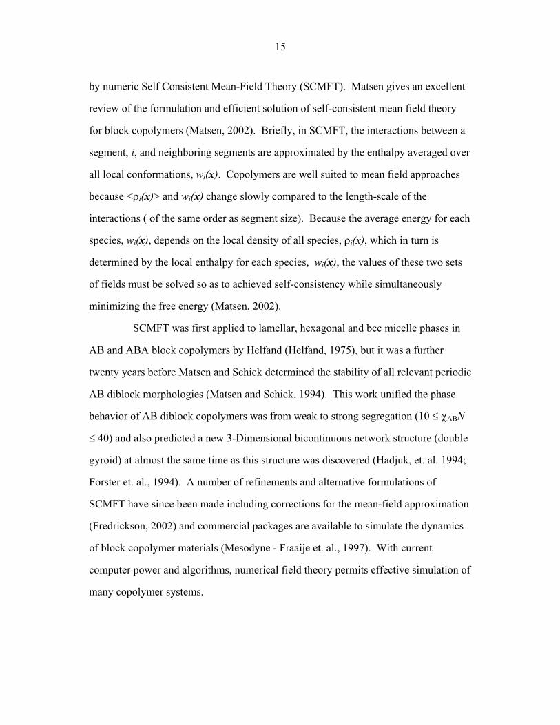
1.4 Diblock Copolymer Morphologies As shown in Figure 1.3, AB diblock copolymers can form several different
morphologies and many years of theoretical and experimental work were required to
understand their phase behavior (Matsen and Bates, 1997). To a good approximation,
AB diblock copolymers have a "universal" phase diagram in which the equilibrium
structure is determined by the block volume fraction fA and block-block interaction
parameter ABN while segment asymmetry (pA ' pB), molecular weight and
polydispersity shift the boundaries between phases.
Figure 1.3- Diblock Copolymer Morphologies. Depending on the volume fraction of A (fA) and interaction parameter (ABN), the A (blue) and B (red) blocks can form spherical (S), cylindrical (C) or lamellar (L) domains. For volume fractions between those cylinder and lamellar structures, the double gyroid (G) network structure can form for some values of the block-block interaction parameter (ABN).
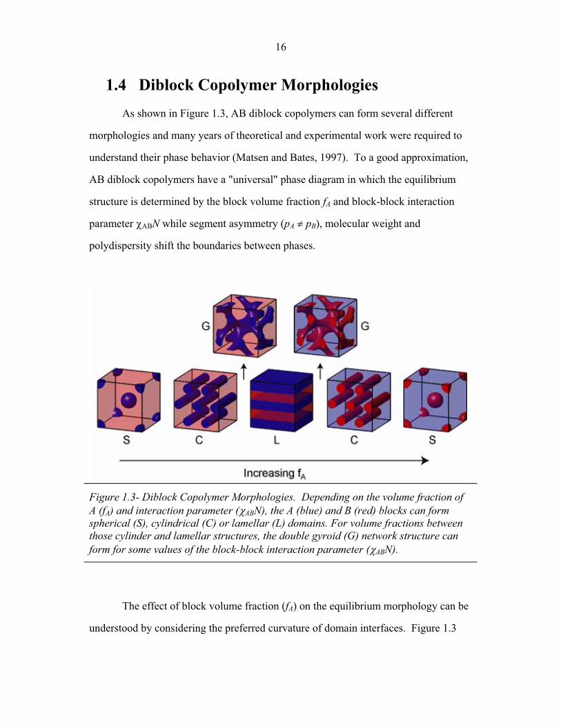
The effect of block volume fraction (fA) on the equilibrium morphology can be
understood by considering the preferred curvature of domain interfaces. Figure 1.3
17
shows an asymmetric block copolymer (fA = 0.25, fB = 0.75) with flat and curved
domain interfaces. If the interface flat (Figure 1.4a), the thickness of the two domains
are proportional to their volume fractions and the thickness of the B domain (dB) is
three times that of the A domain (dA). Curving the domain interface towards the
smaller A domain (Figure 1.4b) reduces chain stretching in the B-domain but increases
chain stretching in the A domain. Thus, the tradeoff between stretching in the A and
B domains leads to an optimal interfacial curvature that depends on the block volume
fractions and packing lengths (pA, pB). In the absence of segment asymmetry (pA =
pB), the optimal interface curves toward the smaller block and the curvature increases
as the block volume fraction decreases (Matsen, 2002; Grason, 2006).
Figure 1.4- Domain Interfacial Curvature. Both panels show an AB diblock copolymer with the same interfacial area and fA = 0.25. (a) At the flat interface the width of the A domain (dA) is one third of that of the B domain (dB). (b) At a cylindrical interface, both domains have the same width.
This trend in preferred domain curvature is reflected in the succession of
"classical" diblock morphologies shown in Figure 1.3. For equal volume fractions (pA
= pB), the A and B blocks form lamellar domains with flat interfaces. At lower
volume fractions of the A or B block, the minor block forms curved cylindrical
18
domains and for the lowest volume fractions the minority block forms even more
micelles (Li, et. al. 2004) and two-dimensional "knitting" (Breiner, et. al. 1998) and
ladder (Kaneko, et. al. 2006) structures.
The larger morphological complexity of ABC triblock copolymers reflects the
increased number of molecular parameters with two independent block volume
19
fractions (fA, fB , fC = 1 - fA - fB) and three block-block interaction parameters (ABN,
BCN and ABN). Changes in interaction parameters can induce morphological
transitions, even when the block volume fractions remain constant. This process is
illustrated in Figure 1.5 for three ABC triblock copolymer morphologies in which the
block volume fractions are all equal (fA = fB = fC = 1/3).
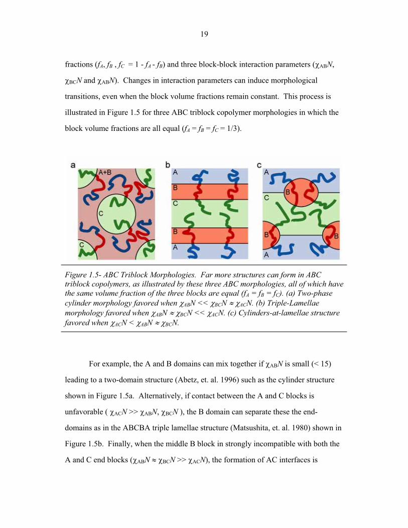
Figure 1.5- ABC Triblock Morphologies. Far more structures can form in ABC triblock copolymers, as illustrated by these three ABC morphologies, all of which have the same volume fraction of the three blocks are equal (fA = fB = fC). (a) Two-phase cylinder morphology favored when ABN << BCN ( ACN. (b) Triple-Lamellae morphology favored when ABN ( BCN << ACN. (c) Cylinders-at-lamellae structure favored when ACN < ABN ( BCN.
For example, the A and B domains can mix together if ABN is small (< 15)
leading to a two-domain structure (Abetz, et. al. 1996) such as the cylinder structure
shown in Figure 1.5a. Alternatively, if contact between the A and C blocks is
unfavorable ( ACN >> ABN, BCN ), the B domain can separate these the end-
domains as in the ABCBA triple lamellae structure (Matsushita, et. al. 1980) shown in
Figure 1.5b. Finally, when the middle B block in strongly incompatible with both the
A and C end blocks (ABN ( BCN >> ACN), the formation of AC interfaces is
20
favored as in cylinders-at-lamellae morphology (Auschra and Stadler, 1993; Figure
1.5c).
Understanding the rich phase behavior of ABC copolymers presents several
theoretical and experimental challenges. Just like AB diblock copolymers, ABC
triblock structures can be well described using SCMFT. However, initial conditions
determine which local minimum is found by SCMFT so it can be difficult to find the
global minimum of free energy (Bohbot-Raviv and Wang, 2000; Fredrickson, et. al.
2002). Experimentally, the synthesis of ABC triblock copolymers is challenging and
presently there are no simple ways to produce a combinatorial library of block
compositions (Bates and Fredrickson, 1999). Furthermore, a three-domain structure
can form via a two-domain intermediate (Yamauchi, et. al. 2003; Maniadis, et. al.
2004) making it especially difficult to determine if an ABC copolymer structure is an
equilibrium morphology (Bates and Fredrickson, 1999).
Given these difficulties, a useful approach has been to study the morphologies
formed in a particular regime. Examples of this include studies on series of ABC
block copolymers with a small middle block (Stadler, et. al. 1995), large middle block
(Mogi, et. al. 1992; Mogi, et. al. 1994; Nakazawa and Ohta, 1993), a single large end
block (Breiner, et. al. 1997) and series in which the size of the C block was varied
(Bailey, et. al. 2001; Bailey, et. al. 2002; Ludwigs, et. al. 2003b). Although the
progression of morphologies in each regime has provided many useful insights, much
of parameter space remains to be explored.
1.6 Structural Templating In several biological materials such as bones and shells, the properties of
biological polymers are augmented through the inclusion of mineral components such
as calcium carbonate or silica (Aizenberg, et. al. 2005). These inorganic materials are
21
integrated at the molecular level with proteins and peptides directing the assembly of
nanometer sized inorganic particles into complex, hierarchical structures (Volcani,
1981; Shimizu, et. al. 1998). As the resulting organic/inorganic composites have
outstanding material properties (Aizenberg, et. al. 2005), there has been considerable
interest in mimicking biological self-assembly processes.
A significant step in this direction was taken at the Mobile Oil Corporation,
where researchers used micro-phase separation in a surfactant solution to synthesize
Figure 1.6 illustrates the general synthetic approach developed in the laboratory of
Professor Uli Wiesner (Templin, et. al. 1997; Simon, et. al. 2001; Jain and Wiesner,
2004). In this approach, solutions of the organic (block copolymer) and inorganic
22
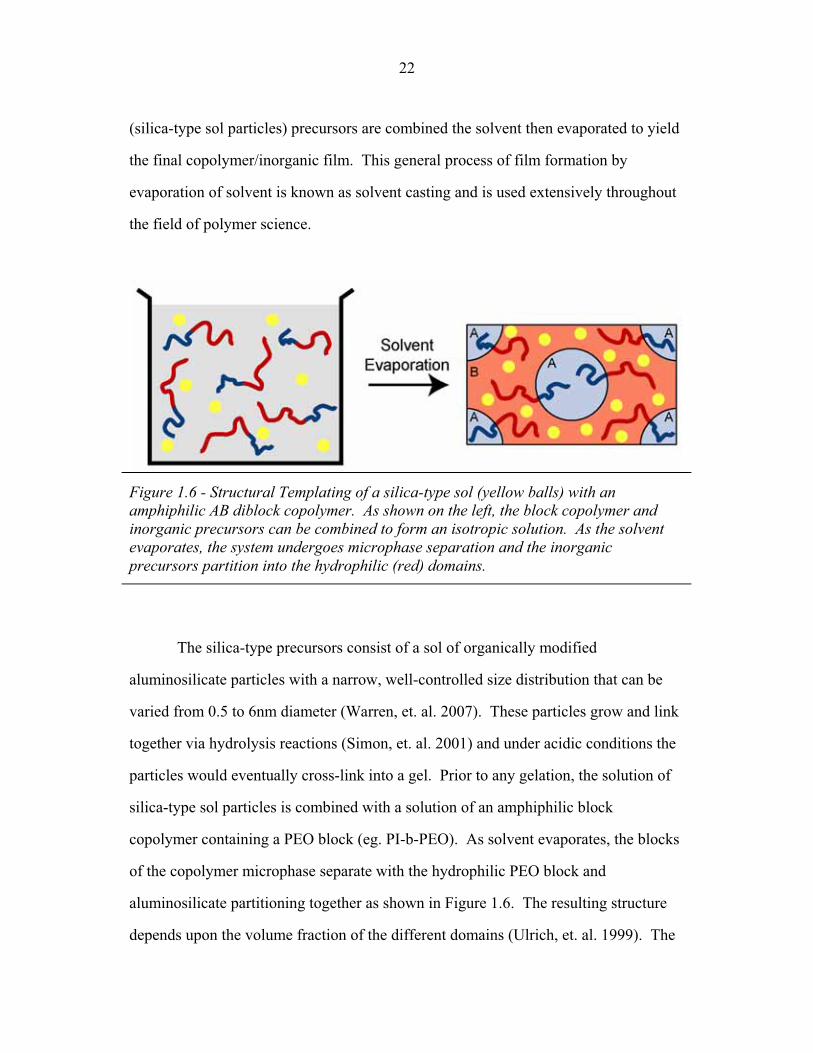
(silica-type sol particles) precursors are combined the solvent then evaporated to yield
the final copolymer/inorganic film. This general process of film formation by
evaporation of solvent is known as solvent casting and is used extensively throughout
the field of polymer science.
Figure 1.6 - Structural Templating of a silica-type sol (yellow balls) with an amphiphilic AB diblock copolymer. As shown on the left, the block copolymer and inorganic precursors can be combined to form an isotropic solution. As the solvent evaporates, the system undergoes microphase separation and the inorganic precursors partition into the hydrophilic (red) domains.
The silica-type precursors consist of a sol of organically modified
aluminosilicate particles with a narrow, well-controlled size distribution that can be
varied from 0.5 to 6nm diameter (Warren, et. al. 2007). These particles grow and link
together via hydrolysis reactions (Simon, et. al. 2001) and under acidic conditions the
particles would eventually cross-link into a gel. Prior to any gelation, the solution of
silica-type sol particles is combined with a solution of an amphiphilic block
copolymer containing a PEO block (eg. PI-b-PEO). As solvent evaporates, the blocks
of the copolymer microphase separate with the hydrophilic PEO block and
aluminosilicate partitioning together as shown in Figure 1.6. The resulting structure
depends upon the volume fraction of the different domains (Ulrich, et. al. 1999). The
23
lamellar, cylindrical and spherical diblock copolymer morphologies have all been
achieved in diblock copolymer/aluminosilicate materials (Simon et. al., 2001).
Throughout the solvent evaporation process, the sol particles continue to cross-
link, especially at the later stages as they become densely packed (Jain and Wiesner,
2004). At the end of the solvent casting process, the aluminosilicate particles are
linked together by a three-dimensional network of covalent bonds. If the composite
material is re-exposed to solvent, the PEO-aluminosilicate domains can retain their
structure. Because the network of covalent bonds within the PEO-aluminosilicate
domain trap the PEO block, the other blocks of the copolymer remain attached even in
the presence of solvent (Ulrich, et. al. 1999). The covalent bonding network within
the PEO-aluminosilicate domains can also preserve its structure when the polymer
component is removed by heating above the polymer above its thermal decomposition
temperature (termed calcination or pyrolysis; Simon, et. al. 2001). Thus, this synthetic
approach provides both block copolymer/aluminosilicate composites and mesoporous
aluminosilicate structures.
Despite considerable progress in this area, many interesting research
opportunities remain, such as adapting the process to other inorganic materials (e.g.
titanium dioxide, silicon carbonitride) and developing methods to position catalytic
particles at the domain interfaces. In addition to these synthetic advances,
improvements in structural control are also important. For example, morphologies
with a three-dimensional network of channels (such as the double gyroid) have
outstanding transport properties but have been hard to synthesize (Hayward, et. al.
2004). Chapter 2 describes the characterization of a network structure formed in a PI-
b-PEO/aluminosilicate composite.
24
Another interesting direction is to use structure-directing agents with more
complex phase behavior than AB diblock copolymers. Linear ABC triblock
copolymers form an enormous number of morphologies but have yet to be widely used
to structure silica-type materials (Mahajan, 2005). Because ABC triblock copolymers
can form three, chemically distinct domains they may be able to simultaneous position
multiple types of inorganic material (Bockstaller, et. al. 2005; Chiu, et. al. 2005).
Chapters 5 and 6 describe two new ABC block copolymer/aluminosilicate structures.
1.7 Small Angle X-ray Scattering Block copolymers have been studied with a wide range of experimental
techniques such as Atomic Force Microscopy (AFM; e.g. Ludwigs et. al., 2005),
rheology (Kossuth et. al., 1999; Cho et. al., 2004), gas permeability (Kinning et. al.,
1987) and dielectric spectroscopy (Ruzette et. al., 2001; Cho et. al., 2004). For
structural studies, two of the most widely used techniques are Transmission Electron
Microscopy (TEM; Thomas and Midgley, 2004) and Small Angle X-ray Scattering
(SAXS; Chu and Hsiao, 2001). The technique of x-ray scattering (Als-Nielsen and
McMorrow, 2001; Warren, 1969) and SAXS (Guinier and Fournet, 1955; Glatter and
Kratky, 1982) are well described in a number of introductory texts and the reader is
strongly encouraged to consult these references in preference to the following
overview of SAXS from block copolymers.
X-rays are electromagnetic waves and X-ray scattering from a material
provides information about the local densities of electrons and atomic nuclei within
that material. In conventional X-ray scattering, the X-ray wavelength (�), sample
thickness and other relevant parameters are chosen such that the majority of scattered
X-rays have the same energy as the incident beam (elastic scattering) and have not
undergone multiple scattering events within the sample. When these conditions are
25
achieved, X-ray scattering from a material can be understood in terms of kinematic
diffraction (Chapter 4, Als-Nielsen and McMorrow, 2001). In kinematic diffraction,
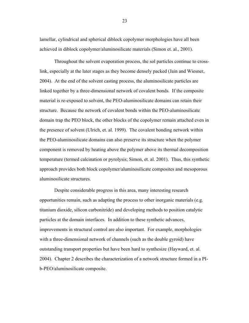
the angle between the incident and scattered radiation (2�; Figure 1.7) is inversely
related to the length-scale being probed. SAXS is a variant of conventional X-ray
scattering in which X-ray scattering close to the incident X-ray beam (typically 2� <
0.1 radians) is used to study ordering at longer length-scales (typically 5 to 100nm).
Figure 1.7 – Schematic of Small Angle X-ray Scattering (SAXS) setup. The sample is inserted into the incident beam of monochromatic X-rays and the intensity of the scattered X-rays is measured with a two-dimensional area detector. X-rays scattered by an angle 2� are detected at a position (x, y) that depends upon the distance between the sample and detector (L). A beam stop prevents the intense, transmitted beam from reaching the detector.
26
Figure 1.7 shows a schematic of typical SAXS setup. The sample is inserted
into a tightly collimated (typical angular divergence < 10-3 radians) beam of
approximately monochromatic x-rays (typical wavelength ��~ 0.15nm). A two-
dimensional x-ray area detector a distance, L, from the sample measures the intensity
of the scattered x-rays as a function of scattering direction while a small beam stop
prevents the intense, transmitted beam from reaching the sensitive X-ray detector. An
example of a SAXS diffraction pattern from an ABC triblock copolymer is shown in
Figure 1.8a.
The direction of scattered x-rays can conveniently be described in terms of the
scattering wave-vector, q, defined as,
incidentscattered kkq &� , (1.13)
where kincident is the wave-vector of the incident X-ray and kscattered is the wave-vector
for the scattered X-ray. Frequently, scattering is described in terms of the closely
related scattering vector, s, defined as,
�2qs � , (1.14)
and the use of q or s is largely a matter of taste. For elastic scattering, the incident X-
ray beam and scattered X-rays have the same wavelength, �) and the magnitude of s is
then given by,
��sin2
�� ss , (1.15)
where 2� is the angle between the incident and scattered X-rays. Thus, for elastically
scattered X-rays the scattering direction determines the scattering vector (s). As noted
above, scattering at small angles probes ordering at longer length-scales (1/s). When
the scattering angle is small (sin(���**�+), the scattering vector can be approximated
by,
27
!"
#$% �( yxs ˆˆ1
Ly
Lx
�, (1.16)
where (x, y) is the position of a point on the detector relative to the transmitted beam.
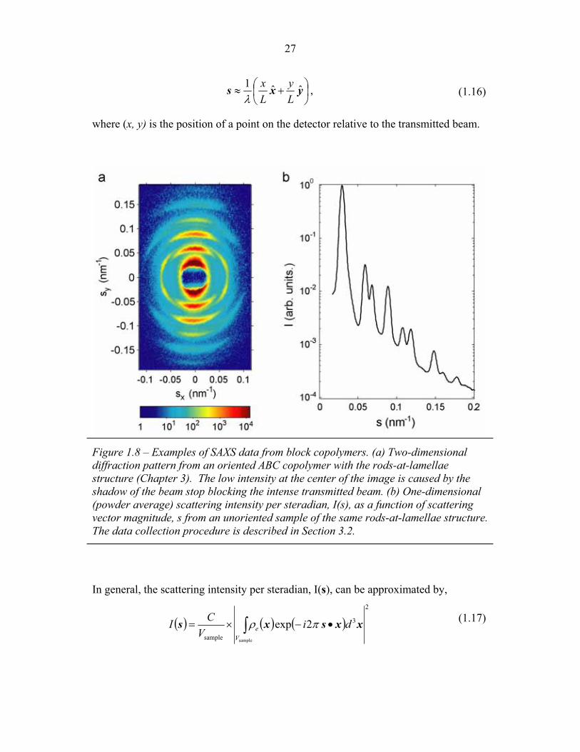
Figure 1.8 – Examples of SAXS data from block copolymers. (a) Two-dimensional diffraction pattern from an oriented ABC copolymer with the rods-at-lamellae structure (Chapter 3). The low intensity at the center of the image is caused by the shadow of the beam stop blocking the intense transmitted beam. (b) One-dimensional (powder average) scattering intensity per steradian, I(s), as a function of scattering vector magnitude, s from an unoriented sample of the same rods-at-lamellae structure. The data collection procedure is described in Section 3.2.
In general, the scattering intensity per steradian, I(s), can be approximated by,
� � � � � �2
3
sample sample
2exp� ,&��V
e diV
CI xxsxs �� (1.17)
28
where C is a constant, Vsample is the volume of the sample and �e(x) is the electron
density at point, x, within the sample. The intensity of scattering, I(s), is determined
by the order within the material with a spatial period of 1/s along the direction of s.
Mathematically, I(s) is proportional to the squared amplitude of the Fourier transform
of the electron density of the material, �e(x). In a crystal, the electron density is
periodic and the scattering intensity is then,
� � � �� � !"#
$% �&�����
lkhhkl VVlkhFCI
,,sample
31
sample32 sbbbs 321� , (1.18)
where a1, a2 and a3 and b1, b2, and b3 are the real and reciprocal lattice vectors defined
as,
jibaba jiii '�,�, for0and1 , (1.19)
while Fhkl is the structure factor defined as,
� � � �� �� ,��&�cell cell
3
2expV
ehkl VdlkhiF xxbbbx 321�� , (1.20)
where Vcell is the volume of the unit cell. Consequently, SAXS from a block
copolymer “single crystal” should only show bright Bragg spots where,
0and 2 '��� hklFlkh 321 bbbs . (1.21)
Such Bragg spots are evident in the SAXS pattern shown in Figure 1.8a. Frequently,
however, the microstructure within a block copolymer consists of many small,
randomly oriented crystallites. For such powder samples, the scattering intensity per
steradian, I(s), depends only upon the magnitude of the scattering vector (s) and the
two-dimensional scattering pattern consists of a series of concentric rings with the
scattering intensity per steradian, I(s), given by,
� � � �� � !"#
$% �&����
��
lkhhkl VVslkhF
sCsI
,,
31
sample3
1
sample2
24 321 bbb��
. (1.22)
29
In such a powder scattering pattern (e.g. Figure 1.8b), the position of the scattering
peaks are given by,
0and 2 '��� hklFlkhs 321 bbb . (1.23)
Although SAXS from an un-oriented sample contains less information than SAXS
from an oriented sample, the position and intensity of the scattering peaks can still be
very helpful when determining the lattice and symmetries of a block copolymer
structure.
Before concluding this section, it is helpful to note several features of
experimental SAXS data from block copolymers. Firstly, as is clear in Figure 1.8,
scattering cannot be measured at the smallest angles because of the beam stop used to
block the intense transmitted beam. The size and angular divergence of the incident
X-ray beam determine the minimum size of the beam stop which in turn sets the
minimum scattering vector (smin) and maximum length-scale (1/smin) that can be
and 1/smin < 100nm owing to a trade-off between the size and brightness of the source.
Secondly, experimental scattering peaks (e.g. Figure 1.8) have a finite width
rather than the delta functions in Equations 1.18 and 1.22. A substantial part of this
width results from instrumental effects including the distribution of wavelengths in the
incident X-ray beam, the finite size and angular divergence of the beam and the point
spread function of the x-ray detector. However, disorder within the block copolymer
structure also contributes to the measured peak width. The dynamics of crystal
formation and growth in block copolymers is much slower than in most small
molecule systems and block copolymer structures can get trapped in poorly ordered,
meta-stable structures. Consequently, reducing variations in crystallite orientation and
30
lattice size can require extended annealing (hours to weeks) at elevated temperature or
in solvent vapor.
Finally, the diffraction pattern from a given block copolymer structure (e.g.
Figure 1.8b) is frequently dominated by one or two very strong scattering peaks. This
effect is largely caused by the relatively broad interfaces between the polymer
domains. Unlike the electron density in a ionic or metallic crystal with small unit cell,
the electron density, �e(x), in a block copolymer structure is a fairly smooth function
of position, x, and so the Fourier transform is often dominated by a small number of
terms.
These three general features are evident in much of the SAXS data presented in
the following chapters. SAXS is a powerful tool for studying the structure of block
copolymers, especially when used in combination with Electron Microscopy and
Electron Tomography (Midgley and Weyland, 2003).
1.8 Summary and Overview of Thesis This chapter has provided an overview of block copolymer physics and the use
of block copolymers to form nanometer-scale structures in inorganic materials. The
remainder of the thesis describes the characterization of structures formed in several
block copolymer and block copolymer/aluminosilicate composite materials.
As described in Section 1.4, the bicontinuous double gyroid morphology can
form in AB diblock copolymers when the volume fraction of the minority phase lies
between that of the cylinder and lamellar phases. In the double gyroid structure, both
the minority and majority phases form continuous, three-dimensional networks and
achieving such a bicontinuous structure in block copolymer/inorganic composite
materials is of interest for applications such as membranes, catalysts and electrodes
(Kresge et. al., 1992; Urade et. al., 2007). Chapter 2 describes the characterization of
31
a bicontinuous AB diblock copolymer/ aluminosilicate morphology prepared by Dr.
Ralph Ulrich (Ulrich, 2000; Finnefrock et. al., 2001). Because the morphology within
the material was deformed during its synthesis, the SAXS data were not consistent
with the symmetry of the double gyroid (Ia3d; Space Group Q230; Hahn, 2002).
However, a distorted double gyroid structure was shown to be consistent with the
observed SAXS and TEM data by estimating the effect of deformation during the
solvent casting process. Models of several other network structures were compared to
the SAXS and TEM data and the double gyroid structure was found to be most
consistent. This result improves upon an earlier analysis of the structure of this
material (Finnefrock et. al., 2001; Finnefrock et. al., 2003) and suggests that diblock
copolymer/aluminosilicate materials and pure block copolymers have similar phase
behavior.
Chapters 3 and 4 describe studies of the phase behavior of ABC triblock
copolymers with a small (fB < 0.5), strongly incompatible (�AC << �AB, �BC) B block
and roughly equivalent A and C blocks (fA ( fB; �AB ( �BC ; pA ( pC). As noted in
Section 1.5, such ABC copolymers can have particular rich phase behavior owing to
competition between the obligatory AB and BC interfaces and the optional AC
interface. Dr. Surbhi Mahajan synthesized a series of ABC triblock copolymers (Ch
4, Mahajan, 2005) with different B domain volume fractions (fB = 0.10, 0.15 and 0.25)
and characterization of these copolymers is described in Chapter 3. In all three
copolymers, the A and C blocks formed lamellar domains while the structure of the B
block depended strongly upon fB. The experimental data were consistent with the B
domains forming lamellae (Figure 1.5b) at the large B block volume fraction (fB =
0.25), rod-like domains (Figure 1.5b) at intermediate B block volume fraction (fB =
0.15) and ball-like domains at the lowest B block volume fraction (fB = 0.10). This
32
sequence of phases agrees with an earlier experimental study of PS-b-PB-b-PMMA
triblock copolymers (Stadler et. al., 1995).
Chapter 4 describes a study of the thermodynamic stability of these
morphologies using the strong segregation limit (SSL) approach of Semenov
(Semenov, 1985). Estimates of the Gibbs free energy of each structure suggest that
when �AC < �AB + �BC, the B domains should form lamellae at the larger B domain
volume fractions (fB), rods at intermediate values of fB, and balls at the smallest values
of fB. This result is consistent with the experimental results described in Chapter 3 and
corrects an earlier SSL analysis performed by Stadler and colleagues (Stadeler et. al.,
1995).
As noted in Section 1.6, there is considerable interest in using the rich phase
behavior of ABC triblock copolymers to direct inorganic precursors into complex
morphologies. Chapters 5 and 6 describe the characterization of two new structures
found in ABC triblock copolymer/aluminosilicate materials synthesized by Dr. Surbhi
Mahajan (Ch 5, Mahajan, 2005). Materials in which the B and C domains had roughly
equivalent volume fractions (fB ( fC) and the volume fraction of the A domain was
small (fA ( 0.1) formed a hexagonally patterned lamellar morphology described in
Chapter 5. This structure appears to be a variation upon a diblock double-lamellae
structure. The B and C domains form lamellae, while the small A domains appear to
reduce their unfavorable (but obligatory) contact with the B domain (�AB��--��AC) by
forming micelles. These micellar A domains appear to form pillars through the
lamellar B domain consistent with the “pillared-lamellae” structure proposed by
Bailey and colleagues (Bailey, et. al. 2001).
Chapter 6 describes an unusual structure found in an ABC triblock
copolymer/aluminosilicate material with block volume fractions (fA = 0.19, fB = 0.32
33
and fC = 0.49) close to those of the “pillared-lamellae” materials. Using electron
tomography, Dr Matthew Weyland determined the complex structure and arrangement
of the electron-dense B domains. The individual B domains formed zig-zag shaped
strands (concertinas). In the bulk material, these wiggly strands were arranged in a
four-layer woodpile structure (Sozuer and Dowling, 1994) in which strands in
successive layers ran in alternate directions and the third and fourth layers of strands
were offset. Such a non-parallel rod stacking structure has not previously been
reported in block copolymers. Unlike the cylindrical domains found in the AB
diblock copolymer cylinder phase, in this material the outside of the strands is formed
from two types of domain (A and C). These A and C domains may prevent efficient
stacking of the strands in a parallel fashion, thereby stabilizing the observed four-layer
woodpile structure. However, the interactions favoring the woodpile structure have
not been unambiguously identified. The new ABC triblock copolymer/aluminosilicate
structures described in Chapters 5 and 6 confirm the complicated phase behavior of
ABC copolymers does indeed permit the synthesis of new copolymer/inorganic
morphologies.
Finally, the results of these studies and potential for further experiments are
discussed in Chapter 7.
33b
34
Chapter Two : Diblock Copolymer/
Aluminosilicate Network Structure
2.1 Introduction Porous, inorganic materials formed using organic molecules have many
applications (Kresge, et. al., 1992). For membranes and catalysts, structures with
continuous networks of pores are particularly useful and these have been formed using
both surfactants (Monnier et. al., 1993; Gao, et. al., 2006; Bagshaw et. al., 1995) and
block copolymers (Zhao et. al., 1998 ; Chan et. al., 1998). This chapter describes a
network structure formed by casting a film (solvent casting) from of a solution with a
diblock copolymer and organically modified ceramic precursors (Templin, et. al.,
1996; Simon et. al, 2001; Finnefrock, et. al. 2001).
Small angle x-ray scattering (SAXS) and transmission electron microscopy
(TEM) showed that the material consists of a powder of relatively large crystallites (~
100 microns). After accounting for shrinkage during solvent casting (Klotz et. al.,
2000; Finnefrock et. al. 2003), individual Bragg reflections could be indexed to
crystallites with a body-centered cubic lattice. In the pure diblock copolymer system,
network structures showed the Ia3d crystallographic symmetry (Space Group Q230)
and double-gyroid morphology (Floudas, et. al., 2001). However, diffraction patterns
from the hybrid material possessed {1,1,0} and {2,0,0} reflections which are
forbidden for the Q230 space-group. An earlier analysis concluded that the material
had the Im3m crystallographic symmetry (Space Group Q229) and suggested the
plumber's nightmare morphology (Huse and Leibler, 1988; Figure 2.20c) was
35
consistent with the structure of the network of pores (Finnefrock, et. al. 2001;
Finnefrock et. al., 2003).
However, as discussed in this chapter, uniaxial compression during the solvent
casting process breaks the symmetries of the original cubic lattice so reflections
forbidden in the original cubic lattice are permitted in the compressed lattice. Indeed,
for models with the double-gyroid morphology, compression leads to significant
{110} and {200} reflections. The experimental structure factors are consistent with
such a distorted double-gyroid model and inconsistent with corresponding models of
the plumber's nightmare morphology. Furthermore, TEM of the material closely
resemble projections of the double-gyroid model while differing markedly from
projections of the plumber's nightmare.
Thus, the simplest model consistent with the experimental data is a double
gyroid morphology with mild distortions caused by solvent casting. This structural re-
assignment suggests that the phase diagram of these copolymer/ inorganic hybrids is
indeed quite similar to that of copolymer/homopolymer blends (Floudas et. al., 2001).
2.2 Experimental Methods
2.2.1 Synthesis
The synthesis of the diblock copolymer/aluminosilicate material performed by
Ralph Ulrich has been described previously (Finnefrock, et. al. 2001, 2003). Briefly, a
poly(isoprene-b-ethylene) oxide (PI-b-PEO) diblock copolymer was prepared by
living anionic polymerization (Molecular Weight of 16.4 kg/mole, Volume/Weight
fraction of PEO of 35%/38%, and polydispersity of 1.07) and is referred to as polymer
V36 in Ralph Ulrich’s PhD thesis (p51, Ulrich 2000). Small Angle X-ray Scattering
36
(SAXS) from the pure copolymer was consistent with a hexagonal morphology with a
unit cell of ~23nm (page 58, Ulrich 2000).
Following the sol-gel protocol developed in the laboratory of Uli Wiesner
(Templin et. al., 1997, Simon et. al., 2001, Jain and Wiesner, 2004), a solution of the
polymer (5% by weight in a (1:1 by volume) chloroform/ tetrahydrofuran mixture)
was combined with a pre-hydrolyzed solution of 3-glycidyloxypropyl
trimethoxysilane (GLYMO) and aluminium sec-butoxide (80:20 by mole). This
solution was transferred to a Petri dish and kept at an elevated temperature (~343
Kelvin) while the organic solvent evaporated over the course of 1-2 hours. After
further annealing of the sample under rough vacuum at ~403K for ~45 minutes, the
final film thickness was approximately 1mm. Assuming the mean density of PI and
PEO-aluminosilicate to be 0.91 g/cm3 and 1.4 g/cm3, the final volume fraction of PI in
the copolymer/aluminosilicate hybrid was 36% (Templin et. al., 1997).
To prepare mesoporous aluminosilicate from the films, the organic material
was burnt out via "calcination". As described in Ralph Ulrich’s thesis (p114, Ulrich
2000), the films were slowly heated (~1K/minute) in air to a maximum temperature of
823K and kept at this temperature for a period of 6 hours before slowly cooling
(~1K/minute) back to room temperature. Following calcination, elemental analysis
indicated the presence of 0.1% by weight carbon and 1.5% by weight hydrogen.
Weight loss following calcinations was 75%, close to the theoretical prediction of
78%. The calcined material was brittle, hard and white.
2.2.2 Gas Adsorption/Desorption
To measure the porosity of the calcined material, nitrogen adsorption and
desorption isotherms were measured at 77K using a Quantachrome Autosorb 6B
(Quantachrome Corportation, Boynton Beach, FL). Samples were out-gassed at 423K
37
and 1mPa for 13h before measurements were made (Finnefrock, et. al. 2001). The
nitrogen sorption isotherm was of type IV according to the BDDT classification with a
specific surface area of 300 m2/gram according to the Brunauer-Emmett-Teller
method (BET; Brunauer, et. al. 1940). Using the Barret-Joyner-Halenda method, the
average pore diameter was calculated to be 8.9nm and the specific pore volume was
0.47 mL/g (Finnefrock, et. al. 2001).
2.2.3 Transmission Electron Microscopy
At the Max Planck Institute for Polymer Physics (Mainz, Germany), Ralph
Ulrich examined thin sections of the material via Transmission Electron Microscopy
(TEM; Finnefrock et. al., 2001). The uncalcined material was used as is, while the
calcined material was manually powdered before embedding the powder in UHU glue
(Henkel). Thin sections of both materials (thickness ~ 100nm) were cut using a
diamond knife Leica-ultramicrotome (UCT) at 218K and sections were floated off the
knife blade onto an aqueous DMSO solution, transferred to EM grids, and examined
without staining. TEM was performed on a Leo 912 . (tungsten filament) operated at
120kV with an objective aperture angle of 16.5mrad. All images were taken in the
elastically filtered imaging mode. To enhance contrast, images were acquired with a
defocus of about 2.5�m. Images were acquired using a slow-scan CCD camera
(1000�1000 pixels, 14-bit ADC). Because of its higher electron density, the PEO-
aluminosilicate phase appears darker than the PI phase in these bright-field images.
2.2.4 Small Angle X-ray Scattering
Small Angle X-ray Scattering (SAXS) data were gathered from both
uncalcined and calcined materials using a laboratory source (Finnefrock et. al., 2001).
Briefly, CuK� x-rays (�=1.54�) were generated with a rotating anode Rigaku RU-
3HR generator (Tube Voltage = 48kV, Tube Current = 58mA, 2mm�0.2mm point
38
focus on a Copper Anode), filtered by a nickel foil (thickness = 10 �m; Goodfellow,
PA) and focused and further monochromatized with a pair of Franks mirrors (Hadjuk,
1994). The flux at the sample was ~4�107 X-rays per second in a beam roughly
1mm�1mm. The x-rays scattered by the sample were imaged with a home-built 2-D
X-ray area detector consisting of a phosphor screen, fiber-optic coupler and
1024�1024 pixel CCD (Tate, et. al. 1995) positioned at the end of an 80cm flight tube.
The much brighter transmitted x-ray beam was blocked with a small circle of lead tape
(typical diameter of 3mm) just inside the end of the flight. The distance from the
sample to the detector and position of the beam center were determined using a silver
behenate calibrant (dl = 5.8376nm; Blanton, et. al. 1995). The scattering measured on
the detector could then be described in terms of the scattering wave vector, q, where q
= |q| = 4��sin�/� and 2� is the total scattering angle. Scattering vectors smaller than q
< 0.1nm-1 could not be measured because of the beam-stop blocking the main beam.
Small flakes of the both the calcined and uncalcined material (~3mm �
~1mm� ~0.5mm) readily “stuck” to the walls of standard x-ray capillaries (diameter =
1.5mm, Charles Supper Co, MA.). To achieve sample rotation about a vertical axis,
x-ray capillaries were suspended with modeling clay from a small AirPax Stepper
Motor that was mounted with double-sided epoxy tape to the top of a motorized X-Y
translation stage. Samples were centered by eye on the stepper motor rotation axis
before acquiring data. For calcined samples, a 90 second exposure was generally
sufficient because of the large density contrast between the aluminosilicate and pores.
Longer exposures of up to 800 seconds duration were required for the uncalcined
material owing to the lower density contrast between the PI and aluminosilicate-PEO
domains.
39
2.3 Results
2.3.1 SAXS
As shown in Figure 2.2 and Figure 2.1, the material produces quite unusual
diffraction patterns where the Bragg reflections lie on ellipses rather than circles.
Furthermore, the eccentricity and tilt of these ellipses varied systematically as the
sample was rotated.
Figure 2.1 - A sequence of SAXS images (90 second exposures) taken from the uncalcined sample at different values of the rotation angle, �, about the qy (vertical) direction. The oligo-crystalline character of the sample is evident from the multitude of distinct Bragg spots seen in each image. The black ellipse marks the position of the {211} reflections as determined by least squares fitting. The eccentricity and tilt of the ellipse varies considerably as the rotation angle is altered.
In Section 2.3.1.1, this ellipticity is accounted for by the anisotropic
contraction of the sample during solvent casting (Klotz et. al., 2000). The magnitude
of anisotropic contraction is quantified, and individual diffraction images are
“rectified” so as to evaluate the powder average of an idealized, uncompressed
sample. After making this correction, the Bragg reflections can be indexed to a body-
centered cubic lattice as described in Section 2.3.1.2.
40
Figure 2.2- A sequence of SAXS images (90 second exposures) taken from the calcined sample at different values of the rotation angle, �, about the qy (vertical) direction. The oligo-crystalline character of the sample is evident from the multitude of distinct Bragg spots seen in each image. The black ellipse marks the position of the {211} reflections as determined by least squares fitting. The eccentricity and tilt of the ellipse varies considerably as the rotation angle is altered.
41
2.3.1.1 Elliptical Diffraction
The elliptical shape of the 2-D diffraction rings can be accounted for within the
following model (Klotz et. al., 2000; Finnefrock et. al. 2003). Samples were prepared
by the slow evaporation of solvent and although the solution is initially quite fluid, as
solvent evaporates and cross-links form within the aluminosilicate, the viscosity rises
so that at the later stages of casting the material is effectively a solid. Because the film
is firmly pinned to the substrate, as the remaining solvent evaporates the film contracts
along the direction perpendicular to the surface. In other words, the film becomes
thinner without a substantial change in its area. The effect of this strain field on
individual crystal domains is depicted in Figure 2.3.
Irrespective of crystallographic orientation, the lattice of each domain is
compressed along the direction of the surface normal. This transformation can be
described by the equation,
ukjk
cj xMx � , (2-1)
where xku is the position of a point before compression, xj
c the position after
compression and Mjk is a 3�3 matrix. For a uniaxial compression the transformation
matrix, Mjk, can be written as,
� � kjkjjkjk nntnnM �&�� , (2-2)
where nj is the surface normal and t is the ratio of compressed film thickness to
uncompressed film thickness. Uniaxial compression in real space leads to uniaxial
expansion in reciprocal space. Before compression, the Fourier transform of the
structure can be defined as,
� � � � � �� &� kllku
ju xdxiqxqF 3exp� , (2-3)
where Fu(qj) is the Fourier amplitude for the uncompressed structure, qj is the wave-
vector and �u(xk) is the electron density at point xk.
42
Figure 2.3 – Cartoon illustrating the effect of sample contraction on crystallites with a cubic lattice. (a) Ideal isotropic case. The orientation of three crystallites is illustrated on the left, while on the right the positions of the {211} reflections are marked in the same color. For a given value of h2+k2+l2, all reflections lie on the surface of a sphere. (b) Following contraction of the sample perpendicular to the substrate, the unit cell of individual crystallites also contracts in this direction. As shown on the right for the {211} reflections, the reciprocal lattice becomes elongated and reflections with a given value of h2+k2+l2 now lie on the surface of a prolate spheroid.
The Fourier transform following film compression, Fc(qj), is then,
43
� � � � � �� � ,
,exp 3
llmu
kmlmlku
jc
qMF
xdxMiqxqF
�
&� � � (2-4)
Thus, film compression transforms points in reciprocal space according to the
equation,
ckkj
uj qMq � , (2-5)
where qju is a point in reciprocal space prior to film compression and qk
c the same
point following film compression. Before film compression, the Fourier transform for
an ideal powder sample would consist of concentric spherical shells. Following film
compression, each of these spheres would be transformed into a prolate spheroid
described by the equation,
20
2222
20
2
20
2
1q
nqtnqq
q
qM
q
q jcjj
cj
cj
ckkj
uj
� !"#
$% &
��� , (2-6)
where q0 is the original radius of the sphere. As illustrated in Figure 2.3b, the spheroid
is stretched along the film normal, nj, by a factor of 1/t.
The 2-D diffraction pattern measured by x-ray scattering is proportional to the
square of the magnitude of the Fourier transform on the surface of the Ewald Sphere.
As shown in Figure 2.4, the shape of a diffraction ring is given by the intersection of a
prolate spheroid and the Ewald Sphere. For these diffraction rings, the angle through
which x-rays scatter is small (< 1�) so the Ewald Sphere may be approximated by a
plane. Equation 2-6 permits direct determination of the diffraction ring shape.
Defining the x-ray beam to directed along the z-axis and the sample rotation axis
about the y-axis (vertical), a point, qj, on the Ewald Sphere can be conveniently
parameterized as,
� �0,cos,sin ��� rj qq , (2-7)
44
where qr is the radius and � the angle from the rotation axis. In the same polar
coordinate system, the surface normal of the sample is,
where �n and �n are the altitude and azimuth of the un-rotated sample.
Figure 2.4 – Cartoon illustrating the intersection of the Ewald Sphere and the prolate spheroid of Bragg Reflections from Figure 2.3. The observed 2-D diffraction ring shape is simply the intersection of the spheroid with the Ewald Sphere shown in (a). For the small scattering angles considered here, the Ewald sphere is approximately a plane. (b) The shape of the scattering ring can be described by an ellipse with semi-minor axis, qmin, and semi-major axis, qmaj, at an angle �e with respect to the y-axis.
Substituting Equations 2-7 and 2-8 into Equation 2-6 gives,
� � � �� �
� � � �
� �� � .costanarctanand,
,sinsin111
,cossin1
0min
2220
maj
22min
22maj2
min2maj
2
nne
nn
eer
qqt
qq
qqqq
q
����
��
����
&��
&�&&�
&�&�
(2-9)
45
The shape of the diffraction ring is an ellipse with a minor radius of length
qmin, major radius of length qmaj, and an angle �e between the major axis and the y-
axis. The same parameterization is also convenient for computing the diffraction
image that would have been observed for the sample in the absence of compression.
Substituting Equations 2-7 and 2-8 into Equation 2-5, a point (qr, �) at radius qr and
angle � on the actual Ewald Sphere correspond to a point (qru, �u) at radius qru and
angle �u on the Ewald Sphere of an uncompressed sample given by,
� �
� � � � � �� � � �� �
.1where
,cos1cos1
coscoscoscos
,cos1
2maj
2min
2222
2
22
qq
qq
ee
eeu
erru
&�
&&�&
&&�
&&�
�
�����������
���
(2-10)
The inverse transformation is given by,
� �
� � � �� �
.sin
11
coscoswhere
,sin1
coscos
,cos1
1
22
2
22
22
2
e
eue
ueu
ueue
ueurur qq
��
���
�������
���
�
&�
�
&&
&�&
&&
��
(2-11)
To apply these equations, the shape of the diffraction ellipses must be
estimated. To illustrate the ellipse-fitting procedure, Figure 2.5 shows the diffraction
pattern from the calcined sample at � = -90 degrees (lower right panel in Figure 2.2).
A convenient parameterization for the ellipse displayed in Figure 2.5 is given by the
equations,
� �� � � �
� �� � � �
,cossin
cos
,cossin
sin
22min
22maj
majmin
22min
22maj
majmin
ee
e
ee
e
qq
qqyy
qq
qqxx
����
��
����
��
&�&��
&�&��
(2-12)
46
where (xe,ye) is the ellipse center, qmaj is the ellipse major radius, qmin is the ellipse
minor radius, �e is the angle between the y-axis and the major ellipse radius and � is
the angle between y-axis and the point (x(�),y(�)).
Figure 2.5 – Diffraction from the calcined material for � = -90 degrees. The bright {211} Bragg reflections all lie on an ellipse marked in black. The major and minor radii of the ellipse are qmaj=0.572 nm-1 and qmin=0.39 nm-1 respectively, while the angle between the rotation axis (vertical) and the ellipse major axis is �e = 61.25 degrees.
The parameters of Equation 2-12 can be obtained to within a few percent
simply by fitting the ellipse by eye. A more precise estimate can be obtained by
measuring the ellipse radii, q(�), as function of angle and then performing a non-
linear fit of this to the elliptical radii given by,
� � � �� �� �
� �� ���
��
��
2
1
2
2
1
2
0
cc
cc
ccq �
!
"##$
%�� (2-13)
47
where,
� � � �
� � � � � �� �
,sincos,cossin
,2
2cos
,sincos
,1
2min
2
2min
22min
2
2
2min
21
2min
2
2
2
0
eeeee
eeeee
maj
emajmaj
ee
emaj
e
e
maj
e
yxbyxa
qqqqqq
c
qb
qac
qb
qac
����
��
����
�&���
&&&��
&�&�
!
"##$
%�&�
(2-14)
and xe and ye describe the offset of the ellipse origin relative to the radial integration
origin. The result for such a fit is shown in Figure 2.6. The black circles show the
radius of the most intense scattering for bins with a width � = 10 degrees. Because
of the large difference between major and minor ellipse radii, it was essential to
precondition the peak finder with an initial estimate of q(�) and this was conveniently
done using the hand-fitted ellipse parameters. q(�) cannot be accurately determined
for the directions in which there are no Bragg Reflections. In all the images, less than
4 bins out of 36 had ill-defined values of q(�) and these bins were identified and
excluded on the basis of their lower peak intensity. The combination of these two
strategies gave a robust fitting procedure.
The ellipse radii and tilt determination illustrated in Figures 2.5 and 2.6 can be
combined with Equations 2-10 and 2-11 to compute the corresponding diffraction
image from the hypothetical state prior to sample compression. As shown in Figure
2.7, following the transformation all diffraction rings assume a circular form. This
transformation also permits a sensible rotational (powder) average to be constructed,
as shown in Figure 2.8.
48
Figure 2.6 – Least Squares Fitting of Diffraction Rings. This image shows the same diffraction data as in Figure 2.5, only in polar (q,�) coordinates. The black circles mark the peak position of the brightest diffraction ring fitted at10 degree intervals. The black line marks the non-linear least-squares best fit of Equation 2-13 to these radii. The major and minor radii of the ellipse are qmaj = 0.569 nm-1 and qmin = 0.389 nm-1 respectively, while the angle between the rotation axis (vertical) and the ellipse major axis is �e = 61.35 degrees. While the results are similar to those obtained by hand fitting (Figure 2.5), least squares fitting is both more precise and less subjective.
49
a
b
Figure 2.7 –Rectification of Diffraction Images. Using Equation 2-10, the diffraction data shown in Figures 2.5 and 2.6 was transformed into the coordinate system of the uncompressed sample. As expected, the transformed diffraction rings form circles in Cartesian coordinates (a) and straight lines in polar coordinates (b). The black lines indicate peaks for even values of h2+k2+l2 of a cubic lattice with unit cell size of 396 Angstroms. Distinct Bragg reflections are visible for h2+k2+l2 = 2, 4, 6, 8, 10, 14, 16, 22 and 24.
50
0 0.1 0.2 0.3 0.4 0.5 0.6 0.7 0.8 0.9 1
101
102
103
q (nm�1)
I (ar
b. u
nits
.)
Figure 2.8 –Powder average of diffraction from calcined sample at � = -90� following transformation to uncompressed coordinates. The dotted lines indicate values of h2+k2+l2 for a body-centered cubic lattice with unit cell size of 39.6nm.
While analysis of individual diffraction patterns is informative, the
compression model can be tested more rigorously by confirming the dependence of
the ellipse parameters on sample rotation angle, �, given by Equation 2-9. Ellipse
parameters were fitted for a sequence of 23 diffraction images from the calcined
sample (of which Figure 2.2 represents a subset). Figure 2.9 illustrates a non-linear
least-squares fit of these data to Equation 2-9.
Data from a rotation series also permits an estimate of the powder pattern from
the “uncompressed” structure. By definition, the power average is given by,
� � � � jq
jju qdqqqF
qqI
j
'''4
1)( 3
'
2
2 � &� ��
, (2-15)
where I(q) is the average scattering factor for radius q. Using Equations 2-4 and 2-5,
Fu(qj’) can be replaced with Fs(qj’) to give,
51
� � � � � � jq
lmkjkjs qdMqqMqF
qqI
j
'det''4
1)( 3
'
2
2 � &� ��
. (2-16)
a
�90 �45 0 45 90 135 180
0.4
0.45
0.5
0.55
0.6
� � (degrees)
q maj
, qm
in (
nm�
1 )
b
�90 �45 0 45 90 135 180
�60
�40
�20
0
20
40
60
� � (degrees)
� e � (
degr
ees)
Figure 2.9 – Ellipse parameter dependence on rotation angle. a) Major (qmaj, circles) and minor (qmin, squares) ellipse radii as a function of rotation angle (�). b) Angle between ellipse major axis and rotation axis (�e) as a function of rotation angle. The black lines indicate the fit to Equation 2-9 for a unit cell of 39.2 / 0.8 nm, cell shrinkage to t = 0.663 / 0.013 and initial orientation of the surface normal (�n=58.4/1.3�, �n = 9.1 / 4.1�).
52
Substitution of Mjk from Equation 2-2 and conversion to polar form (Equations 2-7
and 2-8) gives the simple form,
� � � �� � � � � �� � ,cos1,where
,,4
sin,,,
)(
22
3,
2
�������
��������
����
e
s
g
gddt
gqFqI
&&�
��
!
"##$
%� �
(2-17)
and where |Fs(q,�,�)|2 is directly proportional to the experimentally measured
scattering intensity in polar coordinates.
0 0.2 0.4 0.6 0.8 1
10�2
10�1
100
q (nm�1)
I (ar
b. u
nits
.)
Figure 2.10 –Integrated powder average of diffraction from calcined sample. The dotted lines indicate values of h2+k2+l2 for a body-centered cubic lattice with unit cell size of 39.8 / 1.4 nm.
Applying Equation 2-17 to the rotation series illustrated in Figure 2.2 results in
the approximate powder average shown in Figure 2.10. The dashed lines in Figure
2.10 indicate the radii for even values of h2+k2+l2 for a cubic lattice with a unit cell of
53
39.8 / 1.4 nm. Distinct peaks are evident for values of h2+k2+l2 of 2, 6, 8, 14 and 22,
while clear shoulders are apparent at 4, 24 and a much less pronounced shoulder
appears to be present at 10. Table 2.1 summarizes the peak intensities determined by
fitting the calcined sample powder pattern using the Voigt peak profile (David, 1986).
Although the fit shows some dependence on the peak profile used, the h2+k2+l2 = 6
reflections are at least 5 times more intense than any of the other reflections.
Table 2.1 – Integrated Peak Intensities for Calcined Sample Powder Average shown in Figure 2.10
q (nm-1) h2+k2+l2 {hkl} Multiplicity Integrated
Intensity
<I{hkl}>
0.223 2 {110} 12 0.77 / 0.08 1.5 / 0.1
0.317 4 {200} 6 7.0 / 0.3 28 / 1
0.387 6 {211} 24 100 100
0.447 8 {220} 12 8.6 / 0.5 17 / 1
0.499 10 {310} 24 0 0
0.547 12 {222} 8 0 0
0.591 14 {321} 48 1.34 / 0.2 0.7 / 0.1
0.631 16 {400} 6 0.45 / 0.1 1.8 / 0.4
0.670 18 {330},
{411}
12 + 24 0.51 / 0.1 0.34 / 0.06
0.706 20 {420} 24 0.72 / 0.1 0.7 / 0.1
0.740 22 {332} 24 2.8 / 0.4 2.8 / 0.4
0.773 24 {422} 24 1.3 / 0.1 1.3 / 0.1
0.805 26 {431} 48 0.58 / 0.1 0.29 / 0.04
54
Diffraction from the uncalcined sample was measured for a much smaller set of
rotation angles. Furthermore, because of the reduced electron density contrast, the 90
second exposures used to gather the scattering images in Figure 2.1 do not show the
same wealth of Bragg Reflections. However, the same ellipse fitting procedure can be
applied and the results are summarized in Table 2.2. The sample shrinkage (t � 0.71)
for the as-made material is comparable to the calcined material, while the unit cell
length is ~57% larger than in the calcined material.
Table 2.2 – Ellipse Parameters for the Diffraction Images of the as-made material shown in Figure 2.1
� Unit Cell (nm) qmaj/qmin �e
0� 63.2 0.98 -7.6�
45� 62.5 0.85 -83.2�
90� 61.9 0.71 -83.6�
Table 2.3 – Integrated Peak Intensities for Uncalcined Sample Powder Average shown in Figure 2.11
q (nm-1) h2+k2+l2 (hkl) Multiplicity Integrated
Intensity
<I{hkl}>
0.143 2 {110} 12 0.6 / 0.5 1.4 / 0.9
0.202 4 {200} 6 24 / 1 95 / 5
0.247 6 {211} 24 100 100
0.285 8 {220} 12 5.2 / 0.3 10.5 / 0.6
0.319 10 {310} 24 0 0
55
0 0.1 0.2 0.3 0.4 0.5
10�2
10�1
100
q (nm�1)
I (ar
b. u
nits
.)
Figure 2.11 – Integrated powder average of diffraction from the un-calcined sample. The dotted lines indicate values of h2+k2+l2 for a body-centered cubic lattice with unit cell size of 62.3 / 2.6 nm.
As shown in Figure 2.11, the short exposure times and small number of images
leads to a rather poor powder average. Furthermore, the h2+k2+l2 = 4 peak appears to
be offset towards larger q. Under these circumstances, estimates of scattering
intensities are quite unreliable. However, for the purposes of completeness Table 2.3
summarizes a non-linear least squares fit of the powder scattering curve to Voigt peak
profiles.
2.3.1.2 Indexing Individual Images
As shown in Figures 2.12 and 2.13, distinct Bragg reflections are evident in
individual diffraction images. The angular position of these spots provided additional
information to that obtained via the radial average of traditional powder analysis.
56
Figure 2.12- Small Angle X-ray Scattering from the uncalcined material. Forty-two individual exposures each of 800 seconds duration were summed to obtain the large dynamic range. The white circles indicate the position of 80 individual Bragg reflections determined by least squares fitting.
The position (radius, r = r0, and angle, � = �0) of individual diffraction spots
was estimated manually. Then, in the vicinity of the diffraction spot (|r-r0|< r, |�-
�0|< �), the intensity, I(r,�) was fitted via non-linear least squares to a polar Gaussian
peak sitting on a constant background given by,
� �� � � �
� � � � Br
rrrrr
IrIwwwmww
� !
"##$
%
��&�&
�&&
������
�� 2
20
2
20
22223
0
22exp
2, , (2-18)
where I0 is the integrated spot intensity, r0 and �0 are the radial and angular position of
the peak center, rw and �w are the radial and angular width of the peak and B is a
constant background level.
57
Values of h2+k2+l2 could be assigned unambiguously for h2+k2+l2 � 16 using
the lattice sizes estimated in Section 2.3.1.1. These peaks were then used to refine the
position of beam-center, lattice constant and ellipticity via a least-squares fit, and then
diffraction spot positions were scaled into lattice units. Figures 2.14 and 2.15 show I0
as a function |q|2 following this scaling of qx and qy. The average intensity of spots is
reported in Table 2.4.
Figure 2.13 - Small Angle X-ray Scattering from the calcined material. Twelve individual exposures each of 90 seconds duration were summed to obtain the large dynamic range. The white circles indicate the position of 68 individual Bragg reflections determined by least squares fitting.
58
0 10 20 30 40 50
10�3
10�2
10�1
100
|q|2 (Lattice Units)
Inte
nsity
(no
rmal
ized
)
Figure 2.14 – I(q) versus |q|2 for the 80 Bragg Reflections from the uncalcined material fitted in Figure 2.12. The best fit to the unit cell is 63.3nm with shrinkage of 3.9% at 6� from the vertical. The horizontal error bars indicate the peak-width of the Gaussian diffraction spots, while the vertical dotted lines denote the allowed values h2+k2+l2. Intensities have been scaled relative to the intensity of the strongest Bragg Reflection.
59
0 5 10 15 20 25
10�3
10�2
10�1
100
|q|2 (Lattice Units)
Inte
nsity
(no
rmal
ized
)
Figure2.15 - I(q) versus |q|2 for the 80 Bragg Reflections from the calcined material fitted in Figure 2.13. The best fit to the unit cell is 39.8nm with shrinkage of 8.2% at 16� from the vertical. The horizontal error bars indicate the peak-width of the Gaussian diffraction spots, while the vertical dotted lines denote the allowed values h2+k2+l2. Intensities have been scaled relative to the intensity of the strongest Bragg Reflection.
As-Made Calcined h2+k2+l2 {h k l} aSpots bPowder aSpots bPowder
2 1 1 0 0.4 (6) 0.3 / 0.1 1.3 (6) 1.5 / 0.1
4 2 0 0 8.0 (2) 56 / 2 6.1 (2) 28 / 1
6 2 1 1 100 (14) 100 100 (22) 100
8 2 2 0 16 (6) 8.1 / 0.7 12 (6) 17 / 1
10 3 1 0 - 0 - 0
12 2 2 2 - - - 0
14 3 2 1 1.6 (8) - 3.2 (8) 0.7 / 0.1
16 4 0 0 1.0 (2) - 3.0 (2) 1.8 / 0.4
18 3 3 0/4 1 1 - - - 0.34 / 0.06
20 4 2 0 - - 2.7 (4) 0.7 / 0.1
22 3 3 2 0.9 (10) - 4.7 (12) 2.8 / 0.4
24 4 2 2 0.3 (2) - 1.7 (4) 1.3 / 0.1
26 4 3 1 - - 1.2 (2) 0.29 / 0.04 aAverage Bragg Spot intensity normalized to {211} reflections. The number of spots each {hkl} is given in parentheses. bFit to "pseudo-powder" average of scattering intensity made by summing scattering from a rotation series. The quoted errors are for the non-linear least squares fit and do not include systematic effects.
Although many of the reflections in Figure 2.12 lie along distinct lines (lunes),
the diffraction spots clearly result from multiple crystallites. While a unique indexing
is not possible, assigning diffraction spots to a set of possible crystal domains can
strengthen the lattice assignment. For a given crystallite with reciprocal lattice
vectors, b1, b2 and b3, the reciprocal lattice positions are given by,
61
321hkl bbbq lkh ��� , (2-19)
where (h,k,l) are the lattice indices. For a crystallite with angular mosaic spread of �,
the Bragg condition is approximately satisfied when,
hkl
hkl
qzq ˆ,
-� , (2-20)
where the surface of the Ewald sphere has been approximated by the x-y plane (small-
angle limit). The set of allowed reflections for a crystallite is simply the subset of
(hkl) that satisfy lattice symmetry constraints and Equation 2-20.
�6 �4 �2 0 2 4 6
�6
�4
�2
0
2
4
6
qx (Lattice Units)
q y (La
ttice
Uni
ts)
Figure 2.16 – Hand-alignment of crystallites to diffraction peaks. The blue circles indicate the diffraction peaks in Figure 2.12, while the black asterisks mark the allowed reflections for a bcc lattice with a zone-direction of [320] and a mosaic spread of 8�.
62
Figure 2.16 illustrates the allowed reflections for a crystallite with zone
direction of approximately [320] and a large mosaic spread of 8� corresponding to
roughly 3 standard deviations (average angular peak width of �w ( 2.7�). The allowed
reflections of a crystallite may be aligned with observed diffraction spots by rotation.
A convenient matrix form for the crystallite orientation and subsequent rotation is,
� � ,exp mkljmlnewjk B���B � (2-21)
where �j is the rotation axis, � the rotation angle, �jml the anti-symmetric tensor and
Bjk = [b1, b2, b3] is a matrix of all three reciprocal lattice vectors. To quantify the fit,
the distance of a diffraction spot (qobs) from a reciprocal lattice site was defined in a
weighted, least-squares sense as,
� �
2
2
2
arccos,
!
"
#####
$
% !
"##$
%
�,
� !
"##$
% &�
���hkl0
hkl0
hkl0hklobs
qqqq
qqqq
qd ,
(2-22)
where �q is the radial width (�q~0.05 inverse lattice units) and �� is the angular width
(���~3�) of the average diffraction spot. Initial crystallite orientations were selected
using a divide and conquer algorithm. A first crystallite was oriented so as to match
the maximum number of diffraction spots and spots were assigned to it on the basis of
a distance cut-off. Using the remaining diffraction spots, the process was repeated to
orient the next crystallite. When all diffraction spots had been assigned, the
orientations of individual crystallites were iteratively adjusted to achieve the best
possible fit. The results of this procedure are shown in Figures 2.17 and 2.18.
These assignments are far from unique. In Figure 2.17, the reflections lying
on crystallographic "lunes" were indexed to a single, main crystallite (red - [320]).
Three other crystallites were then sufficient to account for the remaining reflections.
However, some reflections assigned to the main (red) crystallite could also be indexed
63
to these other crystallites. For example, using a different divide-and-conquer
algorithm (Finnefrock, et. al. 2003) Adam Finnefrock indexed the un-calcined material
diffraction peaks to 5 crystallites, as shown in Figure 2.19. However this ambiguity
does not affect the main conclusion that a small number of cubic crystallites can
account for the observed reflections.
�6 �4 �2 0 2 4 6
�6
�4
�2
0
2
4
6
qx (Lattice Units)
q y (La
ttice
Uni
ts)
Figure 2.17 – Indexing of Diffraction Spots from Uncalcined sample SAXS data shown in Figure 2.12. The peaks can be assigned to four crystallites with zone directions red-[320], blue-[311], green-[111] and yellow-[531].
64
�5 �4 �3 �2 �1 0 1 2 3 4 5
�5
�4
�3
�2
�1
0
1
2
3
4
5
qx
q y
Figure 2.18 -Indexing of Diffraction Spots from calcined material SAXS shown in Figure 2.13. The peaks have been assigned to six crystallites with zone directions red-[421], blue-[433], green-[111], magenta-[210], yellow-[331] and cyan-[210].
65
�6 �4 �2 0 2 4 6
�6
�4
�2
0
2
4
6
qx (Lattice Units)
q y (La
ttice
Uni
ts)
Figure 2.19 – Alternative indexing of Diffraction Spots from uncalcined material SAXS data shown in Figure 2.12. The peaks have been assigned to five crystallites with zone directions red-[320], blue-[331], green-[110], magenta-[311] and yellow-[751].
2.3.2 Modeling Structure Factors
There is a strong association between the bicontinuous network morphologies
formed in soft-condensed matter systems and infinite periodic minimal surfaces
(Luzzatti and Spegt, 1967; Scriven, L.E. 1976; Longley and McIntosh, 1983; Thomas,
et. al. 1988; Hyde, 1996). Figure 2.20 illustrates networks related to Schoen’s gyroid
surface (Schoen, 1970) and Schwarz’s D and P surfaces ((Schwarz, 1890).
66
Figure 2.20 - The unit cell of cubic network structures based on Schoen’s G (a, Space Group Q230, Ia3d, p706, IUCr ), Schwartz’s D (b, Space Group Q224, Pn3m, p683,IUCr ),Schwartz’s P (c, Space Group Q229, Im3m, p702 IUCr) and Schoen’s I-WP (d, Space group Q229, Im3m) Infinite Periodic Minimal Surfaces. The green IPMS divides space between the gold and blue skeletal frames, each of which forms a continuous network in all three spatial directions.
These three morphologies have all been observed in soft-matter and can even
occur in a single system (Maddaford and Trokcioglu, 1993). The G, D and P
structures represent merely three out of a multitude of IPMS (eg. Wohlgemuth et. al.,
2001). Non-cubic, bicontinuous network structures were recently observed in block
(Karcher and Polthier, 1996; Strom and Anderson, 1992) in surfactant systems.
However, in studies to date the G, D and P networks appear to be most prevalent.
Comparison between sample diffraction and the structure factors of models is
helpful for elucidating network morphology and Table 2.5 reports the structure factor
magnitudes for models of the G, D, P and I-WP structures developed by Garstecki and
Holyst (Garstecki and Holyst, 2000, 2001, 2002a, 2002b, 2003a, 2003b).
None of these models match the measured structure factors (Tables 2.1 and 2.3
and Figures 2.14 and 2.15). The double diamond structure (Schwarz's D surface,
Figure 2.20b) is a poor candidate because the lattice is not body-centered and requires
the presence of reflections with odd values of h+k+l, such as the intense {111}
reflections. In contrast, the G, P and I-WP structures have BCC lattices. However,
the P structure considered in earlier publications (Finnefrock et. al. 2001; Finnefrock
et. al. 2003) requires the {110} and {200} reflections to be considerably stronger than
the {211} reflections. The I-WP structure is also a poor match because the {211}
reflections should be markedly weaker than the {110} and {200} reflections no matter
whether the minority phase is located on the 4-fold network, the 8-fold network or
both networks (Garstecki and Holyst, 2003b). Finally, while most of the observed
reflections match well with the gyroid, the observed {110} and {200} reflections are
forbidden in the gyroid structure because of the glide planes and screw axes of the
Q230 space-group (p706, IUCR).
68
Table 2.5 : Structure Factors |F{hkl}|2 for Model Network Structures
h2+k2+l2 a,bD aP aI-WP aG c,dGel e,dGCC f,dGCT gExpt
2 100 100 42 - 0.43 28 23 1.5 / 0.1
3 71 - - - - - - 0
4 6.5 89 100 - 1.0 95 96 28 / 1
6 1.3 22 1.4 100 100 100 100 100
8 0 0 5.3 38 41 26 77 17 / 1
9 0.31 - - - - - - 0
10 0.47 0.05 8.6 - 0.08 1.2 7.6 0
12 3.0 0.06 2.5 - 0 0.1 0.9 0
14 0.48 1.4 0.18 0.21 0.21 0.9 3.2 0.7 / 0.1
16 0 1.1 0.62 0.95 0.92 5.0 2.4 1.8 / 0.4
17 2.1 - - - - - - 0
18 0.57 1.95 0.45 - 0.08 2.0 1.5 0.34/0.06
19 1.8 - - - - - - 0
20 0 0 1.3 0.06 0.24 2.4 0.7 0.7 / 0.1
22 1.6 4.0 0.26 0.07 1.1 3.9 0.8 2.8 / 0.4
24 0 3.35 0.03 0.23 0.63 1.8 0.5 1.3 / 0.1
26 0 0 0.66 0.18 0.32 1.6 0.3 0.29/0.04a|F{hkl}|2 for the double diamond (D), plumber's nightmare (P), I-WP and double gyroid (G) models calculated using the parametric functions of Garstecki and Holyst (2003a). For the D, P and G structures the volume of both networks was 18%. For the I-WP structure the volume of the four-fold network was 36%. bIntensities of the {311} and {421} reflections of the D structure were below 0.1%. cElastic model of the G structure (Gel) following 30% uniaxial contraction. d<|F{hkl}|2> averaged over the [100], [110], [111] and [16,9,4] directions. eConstant Curvature model of G structure (GCC) under 30% uniaxial compression. fConstant Thickness model of G structure (GCT) under 30% uniaxial compression. gExperimental values for pseudo-powder average of calcined material.
69
Unlike the structural models in Figure 2.20, the crystallites in the material are
not strictly cubic. Each triclinic crystallite is related to a cubic lattice by a uniaxial
expansion, but the compressed unit cell cannot have all of the crystallographic
symmetries allowed in a cubic unit cell (Sakurai et. al., 2001; Urade et. al., 2007). If
the uniaxial compression is an affine transformation, the original symmetry constraints
on (hkl) are preserved in the triclinic lattice, even though the triclinic lattice lacks
these symmetries. In general, though, reflections in the compressed lattice are not
subject to the same symmetry constraints and the preservation of lattice pseudo-
symmetries depends on both the character and magnitude of the transformation. For
example, Sakurai and colleagues (Sakurai et. al., 2001) reported the appearance of
{110} and {200} reflections when a styrene-butadiene-styrene block copolymer in the
gyroid phase was plastically deformed under tension. In contrast, for the thin films of
surfactant-templated bicontinuous aluminosilicate described by Hayward and
colleagues (Hayward et. al., 2004), only the {211} and {220} reflections of the Q230
lattice were observed despite a uniaxial compression of ~15% during solvent casting.
%. In a more recent study (Urade et. al., 2007) of a double gyroid mesoporous silica
film, the as-made structure did not show the forbidden {110} or {200} reflections
(~7% contraction). However, calcination caused the film to contract by ~40% and
weak {110} reflections were then observed.
To see if a distorted double gyroid structure is consistent with the observed
structure factors, the structural deformations caused by lattice contraction were
calculated for several models. The rheological properties of the block
copolymer/aluminosilicate material varied during the solvent casting process (Jain and
Wiesner, 2004). Initially, when the solvent content was high, the material should have
been able to flow in response to applied stress. As the solvent content dropped, the PI
and PEO-aluminosilicate phases separated to form 3-dimensional, interpenetrating
70
networks. Even though the individual polymer blocks and aluminosilicate particles
could still move within their respective domains, in this liquid crystalline state the
domain topology could not readily change and the bulk material should have exhibited
a solid-like response to applied stress (Kossuth et. al., 1999). In the final stages of
solvent evaporation, the growing, 3-dimensional network of covalent bonds within the
PEO-aluminosilicate domains should have immobilized both the PEO and PI polymer
blocks. If the uniaxial compression occurred after extensive cross-linking of the
aluminosilicate-sol, the deformation should correspond to the response of an
inhomogeneous, elastic solid, as described in Section 2.3.2.1. In contrast, if the
distortion occurred while the individual polymer blocks could move within their
respective domains, the response of the material can be better described using liquid
crystal models (Section 2.3.2.2).
2.3.2.1 Elastic Model of Sample Distortion
This section describes the response of a material with spatially varying elastic
properties to a macroscopic strain field. The material is assumed to have a periodic
structure so following deformation, a point xj, is mapped to a new position Xj(xk),
given by,
� � � ����m
kmk
mjkjkj xiqAxMxX exp , (2-23)
where Mjk is the transformation matrix and Ajm is the Fourier amplitude corresponding
to reciprocal lattice vector qjm. The strain field, ejk(xl), at point Xj(xk) is defined as
(Volume2, p39-3, Feynman, et. al., 1977),
� � � �
� � � � .22
where
,exp21
!
"##$
%&
�����
�& !
"##$
%
00
�00
� �
jkkjjkm
lmj
mk
mk
mj
mjk
ml
ml
mjkjk
j
k
k
jljk
MMqqAqAie
xiqexX
xX
xe
��
�
(2-24)
71
If the elastic response at a given point is isotropic, the stress field, Sjk(xl), is
where �(xl) and �(xl) are the first and second Lame elastic coefficients at point xl
(Volume2, p39-6, Feynman, et. al., 1977). Again, the elastic coefficients are most
simply described by a Fourier expansion,
� � � �
� � � � ,exp
,exp
�
�
�
�
ml
ml
ml
ml
ml
ml
xiqx
xiqx
��
��
(2-26)
because the coefficients �m and �m are easily related to material structure factors.
Substituting Equations 2-25 and 2-26 into Equation 2-27, the stress tensor is then,
� � � �
� � � �.2where
,exp
,�
�
����
&�
pn
pr
nr
mrjk
pll
npjk
nmjk
ml
ml
mjkljk
qqqeeS
xiqSxS
����
(2-27)
The average elastic energy density per unit volume, Ue, is then just,
� � � �
,21
,21 3
�
�
�
�
m
mjk
mjk
V cellmjkljke
eS
VxdxexSU
cell
(2-28)
where Vcell is the unit cell volume. For a given macroscopic transformation, Mjk, and
elastic properties defined by a finite set of reciprocal lattice vectors qjm and Lame
coefficients �m and �m, the distortion amplitudes, Ajm, can be rapidly determined
numerically via conjugate-gradients minimization of Equation 2-28 (Press et. al.,
1986) using the derivative form,
mk
mjkm
j
e qiSAU
�00 . (2-29)
72
Finally, the structure factors following the non-affine transformation can be
determined using the new electron density, �c(Xj(xk)) given by,
� �� � � � xdxXdxX ku
kjc 33 �� � , (2-30)
Equation 2-5 describes the transformation of the reciprocal lattice, while the new
Fourier amplitude Fc(qjmM-1
jk) corresponding to the lattice vector qjmM-1
jk is given by,
� � � � � �� � � �
� � � � � � � �
� � � � � �� � ,
det
,det
expexp
,det
exp
,
1
31
311
M
qqqqFAMiqqF
VMxdxiqAMiqxqqiqF
VMxdxXMiqxMqF
pn
ml
pl
nl
nj
upkjk
mj
mj
u
cellV n pl
pl
pkjk
mjj
mj
nj
nj
u
V cellnkjk
mjl
ujk
mj
c
cell
cell
�
� � �
�
&�&(
!
"##$
%&&�
&�
&
&
&&
�
�
(2-31)
where Fu(qjm) are the Fourier amplitudes of the original structure.
Figure 2.21 illustrates the change in structure factors predicted by Equation
2-31 for a network with the gyroid symmetry following elastic compression. The
uncompressed gyroid structure was assumed to be a constant-thickness membrane
(volume = 64%) separating two networks (Harper, 1996). The reciprocal space
representation of the structure was restricted to wave-vectors with h2+k2+l2 � 64. The
elastic properties of the PEO-aluminosilicate sol and poly(isoprene) phases are
unknown so to estimate an upper bound for elastic effects, the stiffness of the
membrane was taken to be 10 times that of the networks. The value of Poisson’s ratio
does not dramatically alter the results so only calculations for � = 0 are presented in
Figure 2.21. The uniaxial compression was taken to be 70% of the original volume,
and the effects of compression were examined for several directions.
73
Although the structure factors of a gyroid under elastic compression are
qualitatively similar to the experimental results, the magnitude of the {110} and {200}
reflections are about an order of magnitude lower.
0 5 10 15 20 25
10�4
10�3
10�2
10�1
100
h2+k2+l2
<|F
{hkl
}|2 > N
orm
aliz
ed
Original<1,0,0><1,1,0><1,1,1><16,9,4>
Figure 2.21 – Structure factors for a double-gyroid network compressed uniaxially to 70% of its original volume. The gyroid structure was modeled as a constant-thickness membrane separating two networks each of 18% volume. The membrane was taken to be 10 times stiffer than the networks and Poisson’s ratio for both phases was 0. The structure factors following an elastic, uniaxial compression to 70% of the original volume are shown for compression along several different directions. Structure Factors have been normalized relative to the <|F{211}|2>.
74
2.3.2.2 Liquid Crystal Models of Sample Distortion
During hybrid formation, covalent cross-links between aluminosilicate clusters
in the PEO phase transform the material from a fluid to a solid (Jain and Wiesner,
2004). However, even before covalent cross-links immobilize the individual polymer
blocks, the double gyroid structure can exhibit a solid-like response to applied stress
because the major and minor domains form interpenetrating 3-dimensional networks
(Kossuth et. al., 1999). In this liquid crystal state, the shape (but not topology) of
domains can be easily changed because the individual aluminosilicate clusters and
polymer blocks can move within their respective domains. Thus, strain imposed at
intermediate stages of the solvent casting process should cause larger structural
changes than suggested by the elastic model in Section 2.3.2.1. The optimal domain
shapes for a liquid crystal with a given unit cell and domain topology can be used to
estimate the distortion of domains. As the energetic interactions of such a
hybrid/copolymer system have not been quantified, simpler energetic models were
employed.
One approach for describing a network structure is a membrane of uniform
thickness centered on a surface of minimal area (IPMS) (Anderson et. al. 1988; Harper
and Gruner, 2000), where the thickness of the membrane determines its volume
fraction. These "constant-thickness" models are a good approximation for water-rich,
surfactant bilayer network structures and have also been applied to the structure of
block copolymers (Harper, 1996, Garstecki and Holyst 2003a,b). Figure 2.22
illustrates the effect of uniaxial compression on such a constant-thickness model of a
gyroid network. For each structure, the mid-plane of the membrane was described
with a discrete surface (1536 facets per unit cell) and the shape of this surface
optimized numerically to achieve zero mean curvature across it (Brakke, K.A. 1992,
1996 and 2005). The thickness of the membrane was then adjusted to give a volume
75
fraction of 64% and the position of the inner and outer membrane surfaces computed.
Finally, structure factors were evaluated by applying Abbe's transformation to the
discrete representation of the inner and outer membrane surfaces (Harper, 1996).
0 5 10 15 20 2510�4
10�3
10�2
10�1
100
h2+k2+l2
<|F
{hkl
}|2 > N
orm
aliz
ed
Original<1,0,0><1,1,0><1,1,1><16,9,4>
Figure 2.22 – Structure factors for a "constant thickness" IPMS model of a network the gyroid topology after uniaxial compression to 85% of its original volume. As the unit cell is compressed, the IPMS shape changes leading to different structure factors. The results for 15% uniaxial compression along several different directions are presented for a gyroid structure with a membrane volume fraction of 64%.
As expected, an imposed strain can cause larger structural re-arrangements
when material can move within the continuous PI and PEO-aluminosilicate domains.
Indeed, the magnitude of the {1,1,0} and {2,0,0} reflections already matches or
exceeds the observed structure factors for a modest 15% compression. Interestingly,
76
under even larger distortions of the lattice the G surface can be continuously
transformed into either the D or P (Fogden and Hyde, 1999)
Figure 2.23 - Illustration of a single gyroid network under a 15% uniaxial compression along the [16,9,4] direction. Figure 2.23a shows the effect of an affine compression on a surface with constant curvature (enclosing 18% of the unit cell volume) in the original cubic unit cell. Figure 2.23b illustrates the shape of the surface with constant curvature following compression..
Constant curvature surfaces have also been used to describe block copolymer
illustrates the effects of compressing the unit cell for such a structural model. To
calculate the structure factors shown in Figure 2.24, the surface of a single gyroid
network was described with a triangulated surface (2304 facets per unit cell) and the
surface numerically optimized so as to achieve constant mean curvature under the
constraint of a network volume of 18% (Brakke, K.A. 1992, 1996 and 2005). Once
again, the Abbe transform was employed to compute structure factors for the single
network. In the general triclinic lattice, the relative position of the two networks could
77
be ambiguous since the constraints in the cubic case are the glide planes and screw
axes of the Q230 lattice. However, in practice several alternative criteria for positioning
the two networks yield the indistinguishable structure factors.
0 5 10 15 20 2510�4
10�3
10�2
10�1
100
h2+k2+l2
<|F
{hkl
}|2 > N
orm
aliz
ed
Original<1,0,0><1,1,0><1,1,1><16,9,4>
Figure 2.24 –Structure factors for a "constant curvature" model of a network the gyroid topology after 15% uniaxial compression. As the unit cell is compressed, the surface of the network changes to re-establish "constant curvature" leading to changes in the structure factors. The results for a 15% uniaxial compression along several different directions are presented for a gyroid structure with a membrane volume fraction of 64%.
Once again, the magnitude of the {110} and {200} reflections for a
compression of the unit cell by 15% equals or surpasses the magnitudes observed for
the hybrid material. While neither the "constant-thickness" or "constant-curvature"
78
surfaces capture all the details of the copolymer/aluminosilicate hybrid energetics,
they confirm that large changes in structure factor magnitudes may occur without any
change in topology.
2.3.3 Transmission Electron Microscopy
Bright-field transmission electron micrographs of the as-made and calcined
materials are shown in Figures 2.25 and 2.26. Bright areas correspond to the minor
phase (PI or voids) while dark areas correspond to the major phase (PEO and
aluminosilicate). Despite some distortion of the lattice either from solvent casting or
sectioning, both materials show the classic fourfold and threefold orientations of a
cubic lattice. As noted in a published description of these materials (Finnefrock et. al.,
2001), the threefold "wagon-wheels" evident in Figure 2.25c are a common feature of
projections of structural models are frequently helpful (Anderson et. al., 1992; Harper,
1996; Benedicto and O'Brien, 1997). Using published structure factors (Garstecki and
Holyst, 2003a, 2003b), the [100] and [111] projections of the four cubic networks
considered in Section 2.3.2 were evaluated by Fourier summation (Harper, 1996) as
shown in Figures 2.27 and 2.28.
To permit easy comparison of the experimental data with these models, as
illustrated in Figure 2.29, an idealized unit cell was constructed for each micrograph
shown in Figure 2.25. First, the projected lattice vectors were first determined via a
Fourier transform (Figure 2.29b). Following a uniaxial compression along a direction,
nj, the projected lattice vectors of a cubic lattice (size d) are given by,
� �� � klkjkjyyqy
xxxp Rntnnndaaaaaa
A ��&� !
"##$
%�
!
"##$
%� 1
010001
32
321 , (2-32)
79
where Rkl is a unitary 3�3 matrix and t is the fractional length along the compression
axis. Thus,
� � � � � �� � � �
!
"##$
%
&&&&&&&&
� 222
2222
11,11,11
yyx
yxxTpp
ntnntnntnt
dAA , (2-33)
and,
big
smallbig and
��
��� td , (2-34)
where �big and �small are the larger and smaller eigenvalues of Ap�(Ap)T. For each
micrograph in Figure 2.25, the projected lattice vectors, cubic lattice size and
minimum uniaxial compression are reported in Table 2.6. The average lattice sizes
(as-made 53 / 10nm, calcined 36 / 3nm) roughly correspond to the SAXS values
although the apparent lattice size varies considerably between micrographs, especially
for the as-made material. A combination of sample distortion during sectioning,
foreshortened projections and calibration effects frequently lead to such effects in
block copolymer TEMS (Breiner et. al., 1998).
As shown in Figure 2.29a, an array of individual unit cells were then averaged
together to generate a model unit cell (Figure 2.29c). Finally, the lattice was
"rectified" into a cubic lattice as shown in Figure 2.29d. These "rectified" unit cells
are displayed in Figures 2.30 and 2.31 alongside the corresponding projections of the
double-gyroid and plumber's nightmare networks. For the [111] projection (Figure
2.30), the double-gyroid model shows strong similarities to the as-made and calcined
micrographs, while the other network models are quite different. Although the [100]
projection of the G, D, P and I-WP network structures are similar in appearance
(Benedicto and O'Brien, 1997), the G network can be readily distinguished if the unit
cell size is known. As seen in Figure 2.31, the as-made and calcined material match
the gyroid structure.
80
Figure 2.25 – Bright-Field Transmission Electron Micrographs of thin sections (thickness ~ 100nm) of the as-made (top) and hybrid material (bottom) highlighting the threefold (a,c) and four-fold (b,d) projections of the cubic phase. Insets in each panel show the computed Fourier Transform (logarithmic scale) and lattice parameters are given in Table 2.6.
81
Figure 2.26 – Additional Bright-Field Transmission Electron Micrographs of as-made material showing four-fold (a) and three-fold (c) symmetry along with the corresponding Fourier transforms (b and d).
82
Figure 2.27 – Simulated Transmission Electron Micrographs for the [100] orientation of the double-gyroid (a), double diamond (b), plumber's nightmare (c) and I-WP networks (d). All structures have a majority volume fraction (black) of 64%. An area of 2� 2 unit cells is shown in each image and intensity is scaled so that white represents the lowest projected density (minority phase) and black the highest projected density (majority phase). This shading matches that seen for a bright-field TEM. (For the I-WP structure, the minority phase occupies the 4-fold network as shown in Figure 2.20d.)
83
Figure 2.28 – Simulated Transmission Electron Micrographs for the [111] orientation of the double-gyroid (a), double diamond (b), plumber's nightmare (c) and I-WP networks (d). All structures have a majority volume fraction (black) of 64%. Each image has a horizontal width of (8/3)½ and height of 2½ lattice units. The lowest projected density (minority phase) is shaded white and black indicates the maximum possible projected density (majority phase). This shading matches that seen for a bright-field TEM. (For the I-WP structure, the minority phase occupies the 4-fold network as shown in Figure 2.20d.)
84
Figure 2.29 –Averaging and transformation of electron micrographs to produce an idealized unit cell. The original micrograph is shown in (a) along with the 4�6 lattice used to average the unit cell. The unit cell size is determined from the Fourier transform(b), and then the contents of the units averaged as shown in (c). Finally, the intensity can be displayed using basis vectors from a cubic lattice as shown in (d).
85
Table 2.6 - Projected Unit Cell Parameters determined from Micrographs in Figures 2.25 and 2.26.
Micrograph Projected Unit Cell
Vectors (nm)
Apparent Unit
Cell Size (nm)
Minimum Unit
Cell Contraction
Figure 2.25a
As-made [111]
a1 = 32.3 x + 21.1 y
a2 = -31.8 x + 10.5 y
a3 = -0.5x -31.6 y
47.4 22%
Figure 2.26c
As-made [111]
a1 = 45.2 x - 6.3 y
a2 = -15.5 x + 35.3 y
a3 = -29.6x -28.9 y
56.2 18%
Figure 2.25b
As-made [100]
a2 = 40.3 x - 5.8 y
a3 = -37.7 y
42.3 15%
Figure 2.26a
As-made [100]
a2 = 63.8 x -16.5 y
a3 = 15.0 x + 60.9 y
65.9 5%
Figure 2.25c
Calcined [111]
a1 = 26.6 x + 2.0y
a2 = -10.9 x + 15.5 y
a3 = -15.7x -17.5 y
33.4 33%
Figure 2.25d
Calcined [100]
a2 = 36.3 x - 1.4y
a3 = 0x -37.7 y
38.1 5%
86
Figure 2.30 – Comparison of Transmission Electron Micrograph average unit cells (rectified [111] direction) for as-made (a) and calcined (b) with models for the double-gyroid (c) and plumber's nightmare (d).
87
Figure 2.31 – Comparison of Transmission Electron Micrograph average unit cells (rectified [100] direction) for as-made (a) and calcined (b) with models for the double-gyroid (c) and plumber's nightmare (d).
2.4 Discussion Although the bicontinuous character of a material can be inferred by
aCalculated with Equation 3-1 and a segment volume Vref=85cm3/mol=0.141nm3. bInterfacial Tension calculated with Equation 3-2. cInterfacial Thickness calculated with Equation 3-3.
The PEP-b-PEO-b-PHMA copolymers were synthesized by Dr Surbhi Mahajan using
s (nm�1) Figure 3.3 – Scattering intensity per steradian (I) versus scattering vector(s) for Copolymer 1 at 75�C following integration of six exposures (900 seconds). The fit to the scattering profile (Equation 3-4) is marked by the dotted line and can only be distinguished from the experimental data in a few places. The dashed vertical lines mark the allowed peak positions for a lamellar structure with repeat spacing of dl = 48.35 / 0.24 nm. The scattering intensity per steradian (I) is normalized so the strongest scattering corresponds to a value of I = 1 (a. u. stands for arbitrary units).
The dependence of peak width was assumed to take the form,
� �
� � 221
20
221
20
cenggceng
cenglcenl
ss
ss
�����
�����
(3-6)
102
where �l0/�g0 and �l1/�g1 describe the dependence of peak width on scattering angle.
Background scattering was fitted to an inverse polynomial,
� � ��
�3
0kkk
back sB
sI
(3-7)
where Bk are constant coefficients. Results of the fit are summarized in Table 3.5.
Table 3.5 - Peak Parameters of Scattering from copolymer 1 shown in Figure 3.3.
h - Peak Index ascen (� 10-2 nm-1) bscen � dl aI (percent)
1 2.0581 / 0.0026 0.995 / 0.010 100
2 4.1427 / 0.0021 2.003 / 0.010 73.9 / 1.3
3 6.2035 / 0.0040 2.999 / 0.010 6.48 / 0.16
4 8.2596 / 0.0028 3.994 / 0.010 16.32 / 0.36
5 - - -
6 12.426 / 0.010 6.008 / 0.010 1.163 / 0.047
7 14.5172 / 0.0097 7.019 / 0.010 1.414 / 0.051
8 16.541 / 0.047 7.997 / 0.010 0.247 / 0.032
9 18.584 / 0.019 8.986 / 0.010 0.856 / 0.043 aUncertainties for scen and I are from non-linear least squares fit of peak positions. Peak width parameters were �L0 =(5.81 / 0.44) � 10-4 nm-1, �L1 = (1.006 / 0.084) � 10-2, � G0 = (1.562 / 0.031) � 10-3 nm-1 and �G1 = (9.9 / 1.3) � 10-3. bUncertainties for scen � dl are for a least-squares fit of plot of scen versus h. The lamellar repeat spacing is dl=48.35 / 0.24nm.
As is clear from the dotted lines in Figure 3.3, all peak positions can be described by a
single index,
lh d
hs �
(3-8)
103
where dl is the unit cell "height". SAXS for copolymer 1 showed only a modest
dependence on temperature in the range of 50ºC to 200ºC. Below the crystallization
temperature of the PEO block, the lattice size increased discontinuously and the
scattering peaks broadened although the orientation of domains was unchanged.
Previous studies have shown that copolymer morphology can be quite sensitive
to doping with inorganic compounds (Bronstein, L. et. al., 1997; Epps, et. al., 2003).
However, SAXS data from 1-Li (Figure 3.4, Table 3.6) indicate that the morphology
was largely unchanged by the addition of a small concentration of lithium triflate.
s (nm�1) Figure 3.4 - Plot of I versus s for copolymer 1-Li at 60ºC following integration of two exposures (900 seconds). Dashed lines mark peak positions for a lamellar structure with a repeat spacing of dl = 51.25 / 0.26nm.
104
Table 3.6 - Peak Parameters of Scattering from copolymer 1-Li shown in Figure3.4.
h s (nm-1) as � dl I (rel. percent)
1 1.9492 / 0.0023 0.999 / 0.007 95.6 / 1.3
2 3.9260 / 0.0021 2.012 / 0.007 100
3 4.8538 / 0.0045 3.000 / 0.007 8.72 / 0.20
4 7.7936 / 0.0031 3.994 / 0.007 22.42 / 0.34
6 11.707 / 0.019 6.000 / 0.007 1.15 / 0.07 adl = 51.25 / 0.26 nm as determined from linear regression of s versus h.
3.3.1.2 Copolymer 2
In contrast to copolymer 1, scattering from copolymer 2 (Figure 3.5, Table 3.7)
could not be indexed to a single repeat spacing. However, all peaks could be indexed
to a rectangular lattice with peak positions of,
2
2
2
2
clhk d
kdhs ��
(3-9)
where dl and dc and the height and width of the unit cell. The "non-lamellar" {1,1},
{3,1} and {5,1} peaks in Figure 3.5 are quite clear and their positions match the
rectangular lattice. However, the peak intensities in Table 3.7 are not a true powder
average because the intensity of diffraction rings varied around each ring.
Further information about the structure of copolymer 2 was obtained by
preparing oriented specimens. Block copolymer structures can be aligned via electric
Figure 3.5 – Plot of I versus s for Copolymer 2 at 75�C following integration of forty exposures (900 seconds). The observed Bragg peaks can be indexed to a rectangular unit cell (dl = 33.76 / 0.17 nm, dc=16.393 / 0.082 nm). The predicted positions for {h,0} reflections are indicated by black, dashed vertical lines while the {h,1} (h'0) reflections are marked with vertical arrows.
106
Figure 3.6 – 2-D SAXS from an aligned sample of copolymer 2 at 75ºC (logarithmic scale; 36 exposures each of 100 seconds duration). The surface normal was directed along the vertical axis. The (h,0) reflections are located on the vertical axis (sx = h/dl, sy = 0 nm-1) as indicated by the black horizontal layer lines. The (h,/1) reflections also sit on the layer lines but are shifted out onto the vertical row lines (sx = h/dl, sy = /1/dc) for a rectangular unit cell of dl = 33.76 / 0.17nm � dc=16.393/ 0.082nm..
107
Table 3.7 - Peak Parameters of Scattering from copolymer 2 shown in Figure 3.5.
{h,k} ascen (�10-2 nm-1) aI (relative) bscen � dl 2
{6,1} 19.01 / 0.22 0.040 / 0.024 6.420 / 0.010 6.344 aUncertainties for scen and I from non-linear least squares fit of peak positions. Peak width parameters were �L0 =(8.40 / 0.37) � 10-4 nm-1, �L1 = (6.2 / 1.3) � 10-
3, � G0 = (1.887 / 0.033) � 10-3 nm-1 and �G1 = (1.8 / 6.3) � 10-3. bRectangular unit cell size is dl = 33.76 / 0.17 nm by dc=16.393/ 0.082 nm from a weighted least-squares fit of scen
2 versus (h/dl)2+(k/dc)2.
The {h,0} reflections were aligned with the surface normal of the sample and rotation
of the sample about this axis left the diffraction pattern unchanged. This fibre-type
alignment was fairly strong with a width of FWHM=15°. The four sharp peaks off the
vertical axis (sx ( /0.06 nm-1, sy ( /0.03 nm-1) are at the expected positions for the
{1,1} reflections of a rectangular lattice, while the arcs extending from (sx ( -0.06 nm-
1, sy ( /0.09 nm-1) to (sx ( 0.06 nm-1, sy ( /0.09 nm-1) are consistent with the {3,1}
reflections. To improve the estimates of Bragg reflection intensities, the 2-D SAXS
pattern shown in Figure 3.6 was fiber averaged using the form,
108
� �����
��
�����
2
0 4sin
,)(d
sIsI (3-10)
where I(s,�) is the intensity of scattering at a radius s and angle � from the vertical (y-
axis). The average scattering intensity, I(s), was then fitted to Equation 3-4 and the
results are summarized in Table 3.8. No scattering was apparent for either the {0, 1}
or the {h,/2} reflections.
Table 3.8 - Integrated Intensity of Bragg Peaks from Copolymer 2 from Oriented SAXS data shown in Figure 3.6.
{h,k} Intensity (relative)
{1,0} 100
{2,0} 16.80 / 0.35
{1,1} 15.04 / 0.31
{3,0} 15.64 / 0.29
{3,1} 4.56 / 0.13
{4,0} 3.74 / 0.11
{5,0} 1.10 / 0.08
{5,1} 0.18 / 0.06
SAXS from copolymer 2 showed an interesting dependence on temperature as
illustrated in Figures 3.7 and 3.8. When the copolymer was heated, the {h,1}
reflections abruptly disappeared between T=120�C and T=121�C but the {h,0}
reflections remained right up to T = 200�C. Upon cooling of the copolymer, the {h,1}
reflections reappeared at a similar temperature of T ( 120.3 / 0.4�C.
109
0 0.02 0.04 0.06 0.08 0.1 0.12 0.14 0.16
10�3
10�2
10�1
100
101
102
103
119C
120C
121C
122C
{1,1} {3,1}
s (nm�1)
I (ar
b un
its)
Figure 3.7 – Temperature dependence of SAXS from Copolymer 2. SAXS data was gathered as the sample was slowly cooled from 122�C to 119ºC (0.25ºC steps each lasting 30 minutes). For clarity, successive plots of I versus s are offset by factors of 2. {h,0} reflections are indicated by vertical dotted lines (dl = 31.86 / 0.16nm) while arrows mark the {1,1} and {3,1} reflections (dc = 15.73 / 0.10 nm) that appear below T=120.3 / 0.4�C.
110
0 0.02 0.04 0.06 0.08 0.1 0.12 0.14 0.16
10�3
10�2
10�1
100
s (nm�1)
I (ar
b un
its)
{1,0}
{2,0}
{3,0}
{4,0}
{5,0}
{1,1}
{3,1}
Figure 3.8 – Scattering from Copolymer 2 above (dashed; T=122ºC) and below (solid; T=119ºC) the order-order transition. Black dotted vertical lines denote lamellar repeats (dl = 31.86 / 0.16nm) while {1,1} and {3,1} reflections are marked with arrows (dc = 15.73 / 0.10 nm).
Closer examination of SAXS from copolymer 2 above and below the transition
(Figure 3.8) reveals two striking features. Firstly, the {h,0} reflections are essentially
unchanged by the phase transition. This implies that the transition does not effect
structure along the [1,0] direction despite a significant change in order along the [0,1]
direction. Secondly, the sharp {1,1} reflections below the transition are replaced by a
broad scattering feature above the transition (s ( 0.07nm-1), suggesting the presence of
non-crystalline order above the transition temperature.
Below the crystallization temperature of the PEO block, copolymer 2 showed
considerable meta-stability in comparison to copolymer 1. The eventual
crystallization of PEO domains caused a discontinuous increase in lattice size and
111
broadened both the angular and radial width of the scattering to the extent that only
Figure 3.9 – Plot of I versus s for Copolymer 2-Li at 70�C following integration of two exposures (600 seconds). Bragg peaks index to a rectangular unit cell (dl = 34.27 / 0.26 nm, dc=16.951 / 0.085 nm). {h,0} reflections are indicated by black, dotted vertical lines while arrows mark the {h,1} (h'0) reflections.
SAXS from compound 2-Li (Figure 3.9 and Table 3.9) was quite similar to
that from copolymer 2, and the observed diffraction peaks could again be indexed to a
rectangular lattice. The {1,1} and {3,1} reflections appear to be stronger for the
compound 2-Li structure, although this might be biased by grain orientation within the
sample. Another interesting feature is the shoulder (s = 0.083 nm-1) on the side of the
{3,0} peak which corresponds to the expected location of the {2,1} reflections.
{5,0} 14.627 / 0.039 1.40 / 0.19 5.012 / 0.008 5 aUncertainties for scen and I from non-linear least squares fit of peak positions. bRectangular unit cell size of dl = 34.27 / 0.26nm by dc=16.951 / 0.085nm.
The temperature dependence of SAXS from compound 2-Li is shown in Figure
3.10. Previous studies have shown that the addition of lithium triflate to PEO domains
can increase block-block mixing enthalpies (Ruzette, et. al. 2001), and unlike
copolymer 2, in SAXS from compound 2-Li the {1,1} and {3,1} reflections remained
quite strong up to a temperature of 150�C. However, a change in scattering was
observed between 150�C and 170�C that showed similarities to the transition in
copolymer 2. Although the {h,0} peaks did not change significantly, at 170�C the
{3,1} and {1,1} reflections both disappeared, additional scattering was present on both
sides of the {2,0} reflection and the hint of a shoulder appeared on right of the {1,0}
reflection. These changes reversed when the sample was cooled, suggesting they were
not caused by thermal decomposition of the copolymer.
113
0 0.02 0.04 0.06 0.08 0.1 0.12 0.14
10�2
10�1
100
101
102
130�C
150�C
170�C
I (a.
u.)
s (nm�1)
{1,0}
{2,0}
{3,0}
{4,0}
{2,0}
{3,0}
{4,0}
{1,1}
{2,1} {3,1}{2,0}
{3,0}
{4,0}
{1,1}
{2,1} {3,1}
Figure 3.10 – Temperature Dependence of SAXS from compound 2-Li. Plots of I versus s are shown for 130ºC, 150ºC and 170ºC (offset by factors of 10). The {h, 0} reflections are largely unchanged on heating, but at 170ºC the {3,1} and {1,1} reflections cannot be resolved.
114
3.3.1.3 Copolymer 3
SAXS from copolymer 3 at 75ºC is summarized in Figure 3.11 and Table 3.10.
Figure 3.11 – Plot of I versus s for Copolymer 3 at 75�C following integration of four exposures (300 seconds). Dashed vertical lines mark peak positions for a lamellar structure with repeat spacing of dl = 28.44 / 0.14 nm.
The observed Bragg peaks could be described using a single index, although
the fit to the scattering profile was poor in the vicinity of the h=2 peak (s = 0.07nm-1).
Scattering from an oriented sample of copolymer 3 shown in Figure 3.12 revealed the
un-oriented scattering around s = 0.06nm-1 that gave rise to the strange shape of the
h=2 peak shown in Figure 3.11. As shown in Figure 3.12 annealing the copolymer
sharpened the Bragg peaks sufficiently so as to separate them from this scattering
feature. A similar broad scattering feature was present in SAXS from compound 3-Li
115
(Figure 3.13, Table 3.11), although the center of the scattering bump was closer to
s=0.08nm-1. The position and shape of this scattering varied both as a function of
temperature and lithium triflate concentration. Although this scattering definitely
originates from within the copolymer, it is difficult to attribute it to a single source
owing to its broad and rather non-descript character. For instance, an impurity such as
an un-polymerized AB diblock intermediate might form give rise to such scattering,
although no impurities were evident in Gel Permeation Chromatography. As will be
shown in the following section, though, this broad scattering feature could also result
from correlations between disordered domains within the copolymer structure.
Table 3.10 - Peak Parameters of Scattering from copolymer 3 shown in Figure 3.11.
h scen (� 10-2 nm-1) a scen � dl b I (percent)b
1 3.5089 / 0.0020 0.9979 / 0.0029 100
2 6.9170 / 0.010 1.967 / 0.003 1.21 / 0.05
3 10.5393 / 0.0036 2.997 / 0.003 10.22 / 0.18
5 17.589 / 0.015 5.002 / 0.003 1.10 / 0.04 aUncertainties for scen and I are from non-linear least squares fit of peak positions. Peak width parameters were �L0 =(8.19 / 0.98)�10-4 nm-1, �L1 = (1.14 / 0.35)�10-
2, � G0 =(1.22 / 0.10)�10-3 nm-1 and �G1 = (6.9 / 5.9)�10-3. bUncertainties for scen � dl are for a least-squares fit of plot of scen versus h. The lamellar repeat spacing is dl =28.44 / 0.14 nm.
116
Figure 3.12 – Scattering between Bragg Peaks from copolymer 3 (T=75°C). The non-unoriented scattering between the first and second peaks is marked in both plots with an arrow. The upper plot (a) shows scattering from an oriented sample at 0 / 7.5� ( ), 45 / 7.5� (o), and 90 / 7.5� ( ) relative to the lamellar director. The lower plot (b) shows scattering from a powder sample after annealing has sharpened the lamellar peaks.
s (nm�1) Figure 3.13 – Plot of I versus s for copolymer 3-Li at 60ºC following integration of two exposures (600 seconds). Dashed lines mark peak positions for a lamellar structure with a repeat spacing of dl = 28.38 / 0.18nm. Note the broad hump around s = 0.08 / 0.01 nm-1.
Table 3.11 - Peak Parameters for copolymer 3-Li SAXS shown in Figure 3.13.
h scen (� 10-2 nm-1) a scen � dl b I (relative percent) b
1 3.5188 / 0.0044 0.999 / 0.016 100
2 7.113 / 0.025 2.019 / 0.016 2.00 / 0.21
3 10.527 / 0.010 2.988 / 0.016 15.07 / 0.87
5 17.692 / 0.070 5.021 / 0.016 2.24 / 0.44 aUncertainties for scen and I are from non-linear least squares fit of peak positions. bUncertainties for scen � dl are for a least-squares fit of plot of scen versus h. The lamellar repeat spacing is dl =28.38 / 0.18nm.
118
3.3.2 Structure Factor Models
SAXS from copolymers 1, 2 and 3 were compared to simplified structural models of
the triple-lamellae, rods-at-lamellae and balls-at-lamellae structures.
3.3.2.1 Triple-Lamellae
Figure 3.14 - Density profile of the slab model of ABCBA Triple-Lamellae.
The ABCBA triple-lamellae structure can be approximated by a series of slabs of
constant density, as illustrated in Figure3.14 (Epps et. al., 2004). For a unit cell of
period dl, these slabs can be parameterized as indicated in Table 3.12, where �A/B/C is
the density of block A/B/C, fA the volume fraction of block A, wj � dl the width of the
j-th slab and xj � dl the position of the center of the slab.
119
Table 3.12 – Parameters for slab model of the ABCBA Triple-Lamellae Structure
Slab Number - j Density - �j Relative Width - wj Mid-Point - xj
1 �A fA/2 fA / 4
2 �B fB/2 fA/2 + fB/4
3 �C fC 1/ 2
4 �B fB/2 1 - fA/2 - fB/4
5 �A fA/2 1-fA/4
For Copolymer 1 the block volume fractions were fA = 0.34, fB = 0.25 and fC = 0.41 while block densities were approximated with the homopolymer densities �A = 0.86 g/cm3, �B = 1.13 g/cm3 and �C = 1.01 g/cm3 (Table 3.1).
The Fourier coefficients of the structure are then,
� �
� � � �
� � � � � � � � � �CCBCh
AABA
N
jjjjj
dx
x ll
TLh
hffhff
hxihww
ddx
dhxixF
l
������
���
��
sinc1sinc
2expsinc
2exp
1
0
��&�&���&�
&�
!
"##$
% &�
�
�
�
�
�
(3-11)
Alternatively, the middle and an end block may mix to form a single lamellar domain
in a "double-lamellae" structure. The Fourier coefficients for this "double-lamellae"
structure are simply,
� � � �1121 sinc hffF DLh ��� ��&� (3-12)
Using equations 3-11 and 3-12, structure factors were calculated for triple-lamellae
and double-lamellae structures for the block volume fractions of copolymer 1. Results
for room temperature densities and volume fractions are presented in Table 3.13 as
these were similar to those at 75ºC. Broadly speaking, the peak intensities from
120
copolymers 1 and 1-Li are a better match to the triple-lamellae structure than the
double-lamellae structure.
Table 3.13 - Experimental Structure Factors for compounds 1 and 1-Li and corresponding Triple-Lamellae and Double-Lamellae structures.
h aICopolymer 1 bICompound 1-Li cITL dI DL
1 100 95.6 / 1.3 68.0 (-) 100 (-)
2 73.9 / 1.3 100 100 (-) 23.2 (-)
3 6.48 / 0.16 8.72 / 0.20 2.1 (-) 0.06 (+)
4 16.32 / 0.36 22.42 / 0.34 36.5 (+) 6.7 (+)
5 - - 10.5 (+) 3.4 (+)
6 1.163 / 0.047 1.15 / 0.07 3.1 (-) 0.06 (-)
7 1.414 / 0.051 - 3.9 (-) 2.30 (-)
8 0.247 / 0.032 - 0.96 (-) 1.21 (-)
9 0.856 / 0.043 - 0.14 (-) 0.06 (+)
10 - - 2.25 (-) 1.2 (+) aExperimental Intensities for Copolymer 1 from Table 3.5. bExperimental Intensities for Copolymer 1-Li from Table 3.6. cTriple-Lamellae Intensities for block densities at 25�C (Table 3.1) and block volume fractions of copolymer 1 (Table 3.3). Fourier coefficient sign given in parentheses. dDouble-Lamellae Intensities assuming B+C blocks of copolymer 1 mix ideally to form a single domain with uniform density.
Further support for this conclusion can be obtained by computing density
profiles that combine the experimental scattering amplitudes with phases from the
structural models. In general, the calculated electron density profile depends strongly
on the phases that are used. However, the phases of the triple-lamellae and double-
lamellae models only differ for the h = 3 and h = 9 Fourier coefficients. Furthermore,
121
for both models the h = 3 and h = 9 Fourier coefficients are small. Consequently, the
choice of phases has a much smaller effect for this case. Figure 3.15 illustrates the
density profiles for copolymers 1 and 1-Li calculated with the phases from the double-
lamellae model. The use of these phases should bias the reconstructed density profiles
towards the double-lamellae model, yet both profiles show the three distinct density
levels of the triple-lamellae model. Similar results are obtained using the phases for
the triple-lamellae model. Thus, SAXS from copolymers 1 and 1-Li is consistent with
a triple-lamellae structure.
0 0.1 0.2 0.3 0.4 0.5 0.6 0.7 0.8 0.9 1
0.85
0.9
0.95
1
1.05
1.1
1.15
x/dl
� (g
/cm
3 )
Figure 3.15 - Density Profiles for copolymer 1 (solid), compound 1-Li (dashed) and the slab-model of ABCBA triple-lamellae (dotted). Densities constructed using phases from double-lamellae structure and experimental structure factors scaled to the density profile of the triple-lamellae slab model (Table 3.13).
122
3.3.2.2 Rods-at-Lamellae
The cylinder-at-lamellae structure has two AC interfaces per unit cell with a
row of rods at each of these interfaces. As shown in Figure 3.16, the rods in these two
rows can be "aligned" or "staggered". In both structures polymer chains stretch out
from each cylinder of B to fill the surrounding A and C lamellae. The Voronoi cell of
each cylinder bounds the region of space closest to it and the shape of the cell depends
upon the position of rods in the adjacent layers. Consequently, the position of rods in
adjacent layers has a small but significant effect on the energy of the copolymer
structure, and the more rounded hexagonal Voronoi cell of the "staggered" packing
should be favored over the rectangular Voronoi cell of the "opposed" packing.
Figure 3.16 - End-on view of rods-at-lamellae structures with “staggered” (a) and “opposed” (b) rod stacking. Polymer chains stretch out from each rod to fill the bounding Voronoi polyhedron (gray and black lines). The "opposed" stacking (P2mm, Space Group No. 6 IUCr) has a rectangular Voronoi cell while the "staggered" packing (P2mg, Space Group No. 7 IUCr) has a more rounded Voronoi hexagon.
Experimentally, the position of rods within the unit cell is directly linked to the
intensity of the {0,1} reflections. In the "opposed" stacking, the two rods have the
same horizontal position, scattering from the two is in phase and the {0,1} reflections
123
are permitted and likely to be strong. For the "staggered" stacking the two rods are
displaced horizontally by half a unit cell (dc/2) and so scattering from them
destructively interferes and the {0,1} reflections are forbidden. Assuming copolymer
2 has a rods-at-lamellae structure, the absence of {0,1} reflections strongly suggests
the rods have adopted the "staggered" stacking. Quantitative predictions of the
relative intensity of other structure factors require a model for the electron density.
Figure 3.17 - Model of the unit cell of the rods-at-lamellae structure with "staggered" packing. The B domains are treated as two half-ellipses with semi-minor axes of �Adx and �Cdx respectively.
124
Figure 3.17 shows a simple model in which the density within each of the three
domains is a constant and the AB and BC interfacial profiles are approximated by
half-ellipses for ease of calculation. The width and height of the ellipses are related to
the volume fraction of B by,
cl
Byx dd
fdd ������
24 (3-13)
For convenience, the density can be divided into two parts -
a) Lamellar slabs with the width and density of the A and C domains
b) Four half-ellipses with densities of �B-�A or �B-�C depending on the slab
lying under the half-ellipse.
The Fourier coefficients for the structure are then,
� � � � � �� �
� �� �� �
� �� � !
"##$
% &��
!
"##$
%��&�
����&��
clcylBAA
clcylBAA
BAABAACAkrods
hk
dk
dhAffhi
dk
dhAkyffhi
hffffF
,exp
,2exp
sinc
1
0
��
��
������
(3-14)
where y1 is the relative offset between the first and second rods along the y-axis (y1=0
for "opposed" and y1=1/2 for "staggered") and Acyl(sx, sy) is the Fourier transform of
the lower cylinder given by,
� � � � � �
� � � �yyxxCcylCBBC
yyxxAcylABBA
yxcyl
dsdsf
dsdsfssA
,2
,2
,
�����
�����
�&��
&�&��
(3-15)
where �cyl(x,y) is the Fourier transform for a half-cylinder defined as,
� � � � � ���
��
�� ���
����&��2
0
2sin4sinsinccos2exp, dyxiyxcyl
(3-16)
125
Using Equation 3-14, structure factors for the cylinder-at-lamellae model were
calculated for block volume fractions of copolymer 2 and the results are reported in
Table 3.14.
Table 3.14 - Structure factors for Copolymer 2 and "staggered" and "opposed" models of the rods-at-lamellae structure.
{h,k} aIexp b,cIopposed b,cIstaggered b,dIstaggered II
{1,0} 100 100 100 100
{2,0} 16.8 / 0.35 21.8 21.8 22.44
{0,1} - 24.8 0 0
{1,1} 7.52 / 0.16 0.11 22.1 11.2
{2,1} - 15.3 0.42 0.09
{3,0} 15.64 / 0.29 5.6 5.6 12.4
{3,1} 2.28 / 0.07 0.8 7.8 4.9
{4,0} 3.74 / 0.11 3.5 3.5 8.5
{0,2} - 3.6 3.6 0.4
{4,1} - 2.5 1.1 0.0
{2,2} - 1.7 1.7 0.13
{5,0} 1.10 / 0.08 0.44 0.44 2.1
{5,1} 0.09 / 0.03 1.2 0.27 0.7 aExperimental values taken from aligned SAXS pattern of copolymer 2 described in Figure 3.6 / Table 3.8. Note the intensity of {h,1} reflections has been divided by 2 to account for their multiplicity. bCalculations used homopolymer densities at 25�C (Table 3.1), block volume fractions for copolymer 2 (Table 3.3) and unit cell dimensions from Table 3.7. cB-domains assumed to have a circular profile centered on AC interface (dx=dy=7.25nm, �A=�C=0.5). dCalculation for B-domains displaced into C domain (�A=0.3, �C=0.7) with flattened aspect ratio (dx= 6.1nm, dy=8.7nm, dx/dy = 0.7).
126
As expected, there is a considerable difference in structure factors for "opposed" and
"staggered" packings. For the "opposed" stacking the {0,1}, {2,1} and {0,2}
reflections are all be strong while the {1,1} and {3,1} reflections are quite weak. In
contrast, the "staggered" stacking has strong {1,1} and {3,1} reflections which agrees
well with the data for copolymer 2. Furthermore, the B domains are expected to be
flattened (dx<dy) and also displaced into the C-lamellae (�C>�A). These modifications
further improve the correspondence with the experimental results. Thus, SAXS from
copolymer 2 is consistent with a rods-at-lamellae model.
In addition to periodic arrangements, rods in the rods-at-lamellae morphology
can have liquid-like order. Because the B-domains are confined to the AC interfaces,
the in-plane position of B-domains does not affect the density profile along the
lamellar axis a disordered "cylinder-at-lamellae" structure could still possess sharp
Bragg reflections corresponding to the lamellar periodicity. In contrast, liquid-like
ordering of the rods would destroy the {h,1} reflections. The SAXS from such a
disordered "cylinder-at-lamellae" structure can be predicted with the following model.
To compare scattering from periodic and disordered structures, it is helpful to define a
normalized scattering intensity per unit volume,
� � � � � �2
3
sample sample
2exp1� ,&�
Ve di
VI xxsxs �� (3-17)
where �(x) the density and point x in a sample of volume, Vsample. For a periodic
structure this is related to the lattice Fourier coefficients by,
� � 31
31
31
,
312
, samplezsamplec
ysamplekh l
xsamplecell
kh VsVdksVd
hsVFI !"#
$%
!"
#$%
!"#
$% &
!"
#$%
!"#
$% &�� ���s (3-18)
so the powder average is,
127
� � � �
22
2
31
312
,,
where
4
!
"##$
%�
!
"##$
%�
� !"#
$% &���
clhk
hk
samplehksample
kh
cellkh
dk
dhs
sV
ssVFsI�
�
(3-19)
The observed scattering pattern is then the convolution of Equation 3-19 with the
instrumental resolution as shown in Figure 3.18.
For structures in which the rods lack periodic order, the scattering can again be
divided into contributions from density variations along the lamellar axis, and
scattering from the B-domains at the AC interfaces. Since the structure along the
lamellar axis is periodic its contribution can be determined via Equation 3-19.
Scattering from the rods depends upon both the cylinder form factor (Equation 3-15)
and the cylinder-cylinder structure factor. Rods at a given interface will be more
strongly correlated with neighbors within the layer than with rods in adjacent layers.
If the rods are entirely uncorrelated between layers, the scattering from the rods is
given by,
� � � � � � 31
312
,2 samplesamplezlcyxcyly VVsddssAsSI !"#
$%�� �s (3-20)
where S(sy) is the in-plane cylinder-cylinder correlation function and the rods are
assumed to be straight and long. If neighboring rods at an AC interface interact via a
parabolic potential, the correlation function is given by,
� � � �� � � �� �� �� � � �cyoy
yyy dss
sssS
����
����(
222
20
20
sinsinh
sinhcosh
(3-21)
where �0 is the Root Mean Square displacement amplitude of the distance between
nearest neighbors. For a sample with fiber-type alignment along the lamellar axis (x-
axis), the scattering from the rods is given by,
� � � �y
lcyxcylyyx s
ddssAsSssI�
2,),(2
� (3-22)
128
while for a complete powder average the intensity is,
� � � ���
�� ��
����0
2sin,cossin)( dssAsS
sddsI cyl
lc
(3-23)
Using Equations 3-23 and 3-19, the scattering from a disordered cylinder-at-lamellae
structure was calculated and the results are plotted in Figure 3.18.
0 0.02 0.04 0.06 0.08 0.1 0.12 0.14 0.16
10�3
10�2
10�1
100
s (nm�1)
I(s)
(ar
b. u
nits
.)
{1,0}
{2,0}
{3,0}
{4,0}
{5,0}
{1,1}
{3,1}
{4,1}
Figure 3.18 - Comparison of Scattering from rods-at-lamellae structures with ordered (solid) and disordered (dashed) rods. Lattice size and experimental peak shapes correspond to the phase transition of copolymer 2 (Figure 3.8). The cylinder shape was chosen to be a little flat (dx/dy = 0.7) and offset into the C-domain (�A=0.3) while �0=0.125dc was chosen to be comparable to the Lindemann criterion for melting (�0 ~ 10% of nearest neighbor distance; Dash, 2002).
The model SAXS patterns are fairly similar to those observed for temperatures close
to the phase transition in copolymer 2. Thus the temperature dependence of SAXS
129
from copolymer 2 is consistent with an order-disorder transition in which the rods of a
rods-at-lamellae structure switch between a "staggered' and liquid-like ordering.
3.3.2.3 Balls-at-Lamellae
The balls-at-lamellae structure can be treated in a similar manner to the rods-
at-lamellae structure. The B-domains at each AC interface can be approximated by
two half-ellipsoids both of diameter, dy. and heights of �Adx and �Cdx respectively.
These dimensions are related to the lattice size and B-block volume fraction by the
relationship,
bcsl
Bxy dd
fdd ������ sin
2622
(3-24)
where ds is the distance between adjacent balls at the AC interface and �bc is the angle
between the two in-plane lattice vectors. Hexagonal ordering (�bc = 60º) should be
favored when balls interact most strongly with in-plane neighbors, while square
packing (�bc = 90º) is plausible if interactions with balls in adjacent layers are
significant. While there are many stackings of these 2-D arrays of balls, in the
simplest case the unit cell has the same period as the AC lamellar structure. For this
case the Fourier coefficients are,
� � � � � �� �
� �� �� �
� �� �
!
"
##
$
% &�&��
!
"
##
$
% &����&�
����&���
bcs
bc
lsphBAA
bcs
bc
lsphBAA
BAABAACAlkballs
hkl
dkllk
dhAffhi
dkllk
dhAlzkyffhi
hffffF
��
��
��
��
�������
sincos2
,exp
sincos2
,22exp
sinc
22
22
11
00
(3-25)
where y1 and z1 are the relative offset between the balls at the two AC interfaces along
the two in-plane crystal axes, and Asph(sx,syz) is the B-domain domain form factor
given by,
130
� � � � � �
� � � �yzsxxCsphCBBC
yzsxxAsphABBA
yzxsph
sddsf
sdsdfssA
,2
,2
,
�����
�����
�&��
&�&��
(3-26)
where �sph(x, y) is the Fourier transform of a half-ellipsoid defined as,
� � � � � ���
��
��
������
��&��2
0
31
2sin3
sinsin2J
cos2exp, dy
yxiyxsph
(3-27)
The morphology of copolymer 3 could result from a balls-at-lamellae structure
in which the disordered packing of balls suppressed the non-lamellar reflections.
Alternatively, because of the low B-block volume fraction, the B and C domains might
have mixed to form a "double-lamellae" structure.
Table 3.15 - Structure Factors for Copolymer 3 and corresponding Balls-at-Lamellae and Double-Lamellae models.
h aIexp b,cIballs I b,dIballs II b,eIDL
1 100 100 100 100
2 1.21 / 0.05 0.53 0.83 0.39
3 10.22 / 0.18 7.2 12.6 10.8
4 - 0.88 0.13 0.39
5 1.11 / 0.04 0.16 1.33 3.63 aExperimental values for Copolymer 3 given in Table 3.10. bBlock densities and volume fractions at 25°C (Table 3.1 , Table 3.3). cB-domains spherical (dx/dy=1, �A=�C=0.5, ds = (3/8)1/2dl). dB domains flattened (dx/dy=0.8), asymmetric (�A=0.4) and closer (ds = 0.55 * dl). eFor double-lamellae model B and C blocks mix ideally to form a single domain.
Using Equations 3-12 and 3-25, scattering intensities for the double-lamellae
structure and {h,0,0} reflections of the balls-at-lamellae model were calculated for the
block volume fractions of copolymer 3. The results in Table 3.15 indicate that both
models are equally consistent with the observed Bragg Peak intensities.
Figure 3.19 - Scattering from the lamellar order (dashed), diffuse scattering from spherical B-domains (dotted) and total scattering (solid) from a balls-at-lamellae structure. Balls were slightly flattened and asymmetric (dx/dy = 0.8, �A = 0.4, ds = 0.55�dl) while in-plane correlations were approximated by Equation 3-21 with �0=0.2dc. For comparison to scattering from copolymer 3, the fitted peak shape parameters in Table 3.10 were used to describe the width of the lamellar scattering peaks.
Although the "double-lamellae" and disordered balls-at-lamellae structures
have very similar Bragg peak intensities, an ideal "double-lamellae" structure would
have no diffuse scatter while the balls-at-lamellae structure should have a broad ring
due to sphere-sphere correlations. If balls are uncorrelated between adjacent layers,
the normalized scattering intensity from a single "crystal" is,
For example, micellar PEO domains trap lithium ions and have low conductivities,
while lamellar PEO domains have good conductivities because ions can travel easily
in two dimensions.
Figure 3.20 shows the conductivity of 1-Li, 2-Li and 3-Li. At all temperatures
the conductivity of 1-Li was an order of magnitude greater than that of 2-Li which in
turn was an order of magnitude greater than the conductivity of 3-Li. If the B-
domains are micellar in 3-Li, cylindrical in 2-Li and lamellar in 1-Li, this relative
sequence is reasonable.
The conductivity of 1-Li is comparable measurements of bulk PEO doped to
the same concentration of lithium triflate (Caruso, et. al. 2002). The rapid increase in
conductivity around the PEO crystallization temperature (Tm(PEO) ( 50�C) reflects
133
the chains in the B-domains undergoing a transition from semi-crystalline to liquid-
like motion and ordering.
0 50 100 150 20010
�12
10�10
10�8
10�6
10�4
Temperature (�C)
Con
duct
ivity
(S
/cm
)
Figure 3.20 - Ionic conductivity of 1-Li+ ( ), 2-Li+ (o) and 3-Li+ ( ).
The substantially lower conductivity of 2-Li is consistent with the current flow
along and between 1-dimensional, cylindrical B domains. Interestingly, 2-Li showed
134
an even sharper increase in conductivity around the PEO crystallization temperature.
This sharp increase may reflect not only the expected increase in mobility of lithium
ions within the PEO domains, but also a change in PEO domain structure. For
example, conductivity at temperatures below Tm(PEO) would be greatly diminished if
crystallization of PEO chains caused cylindrical B-domains to break into short, worm-
like micelles. Indeed, SAXS did show the domain structure within copolymer 2 was
disrupted by PEO crystallization and once the PEO domains crystallized, only the first
and second order lamellar reflections were observed. Thus, SAXS from copolymer 2
is consistent with melting/crystallization of the PEO domains causing a change in the
structure of the PEO domains. Such a structural change would readily account for the
large jump in conductivity at Tm(PEO). Although the structure of the PEO domains is
not known at low temperature, above the melting temperature of PEO the conductivity
of copolymer 2-Li is consistent with the B block forming 1-dimensional domains.
Finally, the low conductivity of 3-Li is comparable to that measured for AB
diblock copolymers with a micellar conducting block (Soo, et. al. 1999). Because
transport within micellar domains does not determine conductivity, no jump in
conductance at Tm(PEO) is expected. The steady increase in conductance of 3-Li with
temperature is consistent with the effect of temperature on the rate at which ions can
transfer between micelles. If the PEO block in 3-Li mixed with the PHMA block to
form B/C lamellar domains, the mobility of lithium ions in the PEO/PHMA blend
would be reduced but the 2-D character of the domains would aid transport. In other
lithium-containing polymer systems, mixing of the conducting and non-conducting
domains reduced the conductivity by less than order of magnitude (Ruzette, et. al.
2001, Yoshizawa, et. al. 2002). Thus, the low conductivity of 3-Li is more likely to
reflect the trapping of lithium within micellar domains.
135
3.3.4 AFM
At the suggestion of Dr Peter Busch, the surface of copolymer 2 was examined
via Atomic Force Microscopy (AFM).
Figure 3.21 - Atomic Force Microscopy phase image of a thin film of copolymer 2 supported on a silicon substrate. The average spacing between lines is 19 / 2 nm. The color bar indicates the phase angle of the oscillating AFM cantilever.
As the lamellae in solvent-cast films of copolymer 2 were oriented parallel to
the surface, in the absence of surface reconstruction AFM should have probed the in-
plane domain structure. For a cylinder-at-lamellae structure, cylindrical B-domains
would be located approximately 9nm beneath the top of the film with a mean spacing
between rods of approximately 16nm. Although the surface of a rods-at-lamellae
136
structure would be essentially flat, phase-contrast imaging could detect the effect of
the underlying B-domains on materials properties. Figure 3.21 shows a representative
phase-contrast AFM image of a film of copolymer 2. The average spacing between
lines in the image (19 / 2nm) is consistent with the apparent cylinder-cylinder spacing
measured via SAXS. The lines were also present in phase-contrast AFM images of
thicker films of copolymer 2, but were not observed in for films of copolymer 1.
3.3.5 WAXS
A promising route to self-assembled, hierarchical materials is through the
inclusion of polymer blocks with internal structure (Muthukumar et. al., 1997, Ikkala
and ten Brinke, 2001).
Figure 3.22 - Cartoon of structure within the Pn-alkylMA. Parallel backbones (dark, horizontal) are spaced apart by their side-chains (light, vertical). The average distance between backbones is dBB while the side-chains are separated by dCC.
In Pn-alkylMA homopolymers, the difference in polarizability and flexibility
between the methacrylate backbone and alkyl side chains leads to a structure where
rows of aligned polymer backbones are spaced apart by their alkyl side chains, as
illustrated in Figure 3.22 (Beiner et. al., 2002; Beiner and Huth, 2003; Wind, et. al.
137
2005). This ordering has a considerable impact upon polymer dynamics as shown by
dynamic mechanical, dielectric, and NMR spectroscopy (Wind, et. al., 2003). The
molecular-scale ordering in copolymers 1, 2, 3, 5-butyl and 6-octyl was studied via
Wide Angle X-ray Scattering.
Figure 3.23 shows that WAXS from copolymers 1, 2 and 3 is quite similar to
WAXS from a PHMA homopolymer (Beiner, et. al. 2002). The broad peak on the
right corresponds to the side-chain correlations (dCC = 0.49 / 0.01 nm) while the peak
on the left results from backbone-backbone correlations (dBB = 1.34 / 0.03nm).
Scattering from chain-chain correlations in the A and B blocks overlaps with the side-
chain scattering from the PHMA block so the right peak is more intense and the top of
the backbone-backbone peak is shifted slightly with respect to the PHMA
homopolymer (dBB = 14.0nm, Beiner, et. al. 2002).
Table 3.16 - WAXS Scattering Peaks for Copolymers 1, 2, 3, 6-butyl and 7-octyl.
Copolymer dbb (nm) dcc (nm)
1 (T = 75�C) 1.35 / 0.03 0.48 / 0.01
2 (T = 75�C) 1.34 / 0.03 0.49 / 0.01
3 (T = 75�C) 1.33 / 0.03 0.49 / 0.01
5-butyl (T = 50�C) 1.19/0.04 0.48/0.01
2-hexyl (T = 50�C) 1.35/0.03 0.48/0.01
6-octyl (T = 50�C) 1.53/0.04 0.48/0.01
WAXS from copolymers 5-butyl and 6-octyl shown in Figure 3.24
demonstrates the dependence of the backbone-backbone spacing on the length of the
alkyl side-chains. As the length of the side-chains is increased from 4 to 6 to 8
138
carbons, the "mean" distance between backbones increases almost linearly (Table
3.16) while the position of the side-chain correlation peak is unchanged. The variation
of peak position with side-chain length for the copolymers is practically identical that
reported for P-nalkylMA homopolymers (Beiner, et. al. 2002).
0 0.5 1 1.5 2 2.5
0.3
0.5
0.7
1
2
3
4
s (nm�1)
I (a.
u.)
CCBB
1
2
3
Figure 3.23 - WAXS spectra for Copolymers 1 ( ), 2 (o) and 3 ( ) at T=75°C illustrating correlations from both carbon chains (CC, right peak, dCC = 0.49 / 0.1nm) and Pn-hexyl-MA backbones (BB, left peak, dBB = 1.34 / 0.03nm). Curves are offset by factors of 2.
139
0 0.5 1 1.5 2 2.5
0.3
0.5
0.7
1
2
3
s (nm�1)
I (a.
u.)
CCBB
Figure 3.24 - WAXS spectra for 5-butyl ( ), 2-hexyl (o), and 6-octyl ( ) at T=50°C illustrating the dependence of Pn-alkyl-MA backbone structure on alkyl side chain length. The mean Pn-alkyl-MA backbone (BB, left peak) spacing increases as the alkyl side-chain length grows while correlations between carbon chains (CC, right peak) are largely unaffected.
3.4 Discussion Although block copolymer morphology is frequently determined using a
combination of electron microscopy and SAXS, electron microscopy was challenging
for these block copolymers. Firstly, because the glass temperature of all three blocks
is below room temperature, the structure of thin sections is only preserved at
cryogenic temperatures and a cryo-EM stage was not available. Secondly, PEP-b-
140
PEO-b-PHMA copolymers cannot readily be stained with RuO4 or OsO4 and contrast
between the unstained blocks is poor. Despite this restriction, SAXS, ionic
conductivity data and AFM provided strong constraints on the morphology of
copolymers 1, 2 and 3. SAXS gave strong support for lamellar ordering in all three
materials while distinct differences in B-domain structure were indicated by the
dramatic differences in the ionic conductivity of each material.
For copolymer 1 the experimental data provides good support for a triple-
lamellae structure. SAXS showed only lamellar peaks and the intensity of the peaks
were comparable to those from the electron density profile of a triple-lamellae model.
Furthermore, the relatively high conductivity of compound 1-Li was consistent with
charge transport in two-dimensional lamellar domains.
SAXS data from copolymer 2 could be indexed to the rectangular lattice of the
rods-at-lamellae morphology (Aushra and Stadler, 1993; Liu et. al., 2003) and the
intensity of the Bragg reflections matched with model structure factors. Confinement
of charge transport to the one-dimensional cylindrical domains of the rods-at-lamellae
structure should reduce conductivity as was observed for compound 2-Li. Finally, the
one-dimensional periodic structure at the surface of copolymer 2 matches that
expected for cylindrical B-domains at the AC interface. Thus, the rods-at-lamellae
morphology is in accord with the experimental data from copolymer 2.
The morphology of copolymer 3 is not as tightly constrained by the
experimental observations. Although SAXS clearly indicates lamellar ordering, the
intensity of the lamellar peaks is consistent with both the balls-at-lamellae (Beckmann
et. al., 1994; Erhadt, et. al. 2001) and double-lamellae structures. However, several
points favor the balls-at-lamellae structure. Firstly, scattering from disordered balls in
a balls-at-lamellae structure should produce a diffuse ring similar to the one observed
141
from both 2 and 2-Li. If copolymer 3 had the double-lamellae morphology this
scattering would imply the presence of an impurity that was not detected via Gel
Permeation Chromatography. Secondly, the very low conductivity of compound 3-Li
favors the balls-at-lamellae morphology in which lithium ions are trapped inside
micellar domains. A double-lamellae structure would have a much higher
conductivity unless lithium ion mobility in the mixed PEO/PHMA phase was
tremendously lower than has typically been observed for other mixed copolymer
phases.
Finally, the large enthalpy of mixing for the B and C blocks favors the balls-at-
lamellae structure. From Hildebrand Solubility parameters the estimated Flory-
Huggins interaction for the B and C blocks was BCN ( 65. While this number is
approximate, the observation of an ordered BCC micelle phase in a PEO-PHMA
diblock copolymer (Mahajan et. al., 2003) provides a firm lower bound of BCN 2 43.
This large enthalpy of mixing would make micelle formation likely even if the B-
domain were an end-block in a diblock copolymer (Matsen and Bates, 1996) and
micelle formation should be more favorable for the B domains in an ABC copolymer.
Firstly, in a double-lamellae structure the AB junction is already constrained at the A-
domain interface so micelle formation incurs a smaller loss of positional entropy.
Secondly, A and B domains must mix at the lamellar interfaces of the double-lamellae
structure. Micelles reduce this very unfavorable interaction between A and B (ABN (
170) as well as less costly mixing B and C domains so the reduction in enthalpy is
greater than would be estimated from BCN alone. Both of these effects favor de-
mixing of B and C domains to form a balls-at-lamellae structure. Although other
structures are possible, the most likely morphology for copolymer 3 is the balls-at-
lamellae structure.
142
Thus, the most likely morphologies for copolymers 1, 2 and 3 are respectively
the triple-lamellae, rods-at-lamellae and balls-at-lamellae structures. This same
sequence of structures was previously observed in PS-PB-PMMA copolymers (Stadler
et. al., 1995).
In addition to the morphological transitions, the ordering of rod-shaped B-
domains in copolymer 2 has not reported in previous studies of the rods-at-lamellae
structure (Auschra and Stadler, 1993; Stadler et. al. 1995; Liu et. al. 2003). A
staggered stacking of rods should minimize chain stretching in the A and C domains
and SAXS confirms this is the arrangement within copolymer 2 at 75�C. The
disappearance of order at higher temperatures is also quite interesting. Transitions
between two and three domain morphologies have been the subject of both theoretical
(Abetz, et. al. 1996; Manniadis, et. al. 2004) and experimental study (Neumann, et. al.
1996; Yamauchi, et. al. 2003). However, mixing of cylindrical B domains with
lamellar C domains to form B/C lamellae may not be the best explanation for the
transition in copolymer 2. In general, a transition from a rods-at-lamellae structure to
a double-lamellae structure would alter the unit cell size and the density profile along
the lamellar axis. Such changes are not observed and the diffuse scatter seen above
the transition temperature (eg. Figure 3.8) is also not expected for a double-lamellae
structure.
For micellar structures in AB diblock copolymers, melting the BCC crystalline
stacking of micelles leads to a disordered liquid of micelles rather than an isotropic
mixture (Domindontova and Lodge, 2001; Wang et. al. 2002). By analogy, above the
transition temperature of copolymer 2, cylindrical B-domains could remain at the AC
interfaces with the position of rods at successive interfaces uncorrelated. In good
agreement with the experimental data, such a transition would leave the density profile
143
along the lamellar axis largely unchanged while diffuse scattering would result from
the liquid-like ordering of cylindrical B-domains. Finally, this transition in the rods-
at-lamellae structure may be particularly interesting because the one-dimensional
cylindrical domains are confined at the AC interfaces along the lamellar axis, but free
to move in the other direction. Dimensionality has important effects on melting
(Dash, 2002; Angelescu, et. al. 2005), and this transition would be an intermediate
between two and one-dimensional melting.
3.5 Conclusion This chapter has examined the effect of reducing the volume fraction of the
middle PEO block (fB) in a series of three PEP-b-PEO-b-PHMA copolymers with
roughly equivalent A and C blocks (fA ( fC). For all three copolymers, SAXS
supported a lamellar arrangement of the A and C domains while ionic conductivity
measurements indicated pronounced differences in the state of the B-blocks. The
experimental data were consistent with the B-block forming lamellar domains at the
largest middle block volume fraction (fB=0.25), rod-like domains at intermediate B
block volume fractions (fB=0.15) and ball-like domains at the lowest B block volume
fraction (fB=0.1). This sequence of phase transitions was previously observed in PS-b-
PB-b-PMMA copolymers (Stadler, et. al. 1995).
144
Chapter Four - Thermodynamics of
Lamellar ABC Structures
4.1 Introduction This chapter examines the thermodynamic properties of ABC block copolymer
structures in which the A and C blocks form lamellar domains. The stability of the
triple-lamellae, rods-at-lamellae and balls-at-lamellae structures (Figure 3.1) has
previously been studied using the Strong Segregation Limit (SSL) approach of
Semenov (Stadler et. al., 1995) and the SSL density functional approximation of Ohta
and Kawasaki (Zheng and Wang, 1995). However, several results of the analysis by
Stadler and colleagues (Stadler et. al., 1995) conflict both with physical intuition and
the conclusions of Zheng and Wang (Zheng and Wang, 1995). Subsequent
computational studies using density functional theory (Bohbot-Raviv and Wang,
2000) and self-consistent mean-field theory (Tang et. al., 2004) did not resolve these
differences as only two-dimensional morphologies were studied. Reexamining the
SSL behavior of the triple-lamellae, rods-at-lamellae and balls-at-lamellae structures
can resolve these differences and also provide a better understanding of the transitions
between the three morphologies.
In this chapter, the Gibbs free energies per copolymer of these morphologies
are estimated using Semenov's SSL formulation of block copolymer free energy
(Semenov, 1985). The SSL formalism is developed in Section 4.2 and is applied to
the triple-lamellae morphology in Section 4.2.1. When the interfacial tension between
the end blocks is smaller than the combined interfacial tension of the AB and BC
interfaces (�AC<�AB+�BC), decreasing the B block volume fraction (fB) destabilizes the
145
lamellar B domain of the triple-lamellae structure. This instability of the lamellar B
domain is described in Section 4.3. More detailed descriptions of the rods-at-lamellae
(Section 4.3.1), balls-at-lamellae (Section 4.3.2) and perforated-lamellae (Section
4.3.3) structures are developed to determine the onset of this transition. In addition to
these lamellar morphologies, Stadler and colleagues also considered a rings-at-
cylinders morphology and this is modeled in Section 4.3.4. In Section 4.4, the
approximate Gibbs free energy per copolymer of each morphology is studied and used
to construct a SSL phase diagram. When �AC < �AB+�BC, the triple-lamellae structure is
optimal for the larger values of B volume fraction (fB), the rods-at-lamellae structure at
intermediate values and the balls-at-lamellae structure is stable for the lowest values of
fB. The predictions of these SSL models are also compared to the three PEP-b-PEO-b-
PHMA copolymers examined in Chapter 3.
4.2 Strong Segregation Limit Formulation In the SSL (ijN � 1), each block of the copolymer chain resides within a
distinct domain while junctions between blocks are localized at domain interfaces, as
shown for the triple-lamellae structure in Figure 4.1. In this limit, the Gibbs free
energy per copolymer may be approximated by (Semenov, 1985),
stretchint GGG �� , (4-1)
where Gint describes the enthalpy of mixing at domain interfaces and Gstretch the loss of
entropy from chain stretching within each domain. When the domain size is much
greater than the interfacial thickness, the interfacial energy is given by,
cell,,int V
VATkGjiji
ijijB ���� �'
, (4-2)
where kB is Boltzmann's constant, T is the temperature, kBT��ij is the interfacial free
energy per unit area between blocks i and j, Aij is the area of domain interfaces
146
between blocks i and j per unit cell, Vcell is the volume of the unit cell, and V the
molecular volume of the copolymer. In addition to the unit cell volume (Vcell), it is
convenient to describe the size of the block copolymer structure in terms of a linear
dimension, d, commonly taken to be one of the lattice dimensions (eg. d = dl for a
lamellar structure and d = dcyl for a cylindrical structure). Defining the coefficient,
�'
��
jiji
ijij
VdA
C,, cell
int 2, (4-3)
the interfacial free energy may then be written as,
dVCTkG B
2intint ��� . (4-4)
Increasing the size of the structure (d) reduces the interfacial energy per copolymer.
Turning to the second term in Equation 4-1, the value of Gstretch depends upon
the average stretching of the individual blocks. For a strongly stretched, continuous
Gaussian chain, the stretching energy is given by (Matsen, 2002),
���j j
jjB
VfRpTkG
2
stretch 23
, (4-5)
where pj is the packing length (Fetters, et. al. 1994), fj the volume fraction and Rj is
the average root mean square path length of the j-th block. The packing length, pX,
characterizes the persistence length of a given type of polymer and is defined by the
relationship (Fetters, et. al. 1994),
2X
X
LVp � , (4-6)
where VX is the chain volume and LX is the root mean squared end-to-end length of the
chain in a homopolymer melt. For a continuous Gaussian chain, the path of a given
polymer backbone can be described by the function, rj(u), in which u is the fractional
distance along the backbone (0 � u � 1; ends of polymer chain at rj(0) and rj(1)). The
average root mean square path length, Rj, is then defined as,
147
� �
� �ur
u
u
jj
j
dudu
udrR �
�
� !
"##$
%�
1
0
22
, (4-7)
where the average is taken over all polymer paths within the domain. The set of the
polymer paths within a domain depends upon how each end of the chain is constrained
(free / tethered at a domain interface) and the spatial distribution of chain ends at the
domain interfaces (Matsen, 2002). Defining the coefficient,
��j j
jj
dfRp
C 2
2
stretch 23
, (4-8)
the energy for the chain stretching may be written as,
Vd
CTkG B
2
stretchstretch ��� . (4-9)
The chain stretching energy increases with the square of the unit cell size (d).
Substituting Equations 4-4 and 4-9 into Equation 4-1, the Gibbs free energy
per copolymer can be expressed as,
Vd
CdVC
TkG
B
2
stretchint2
���� . (4-10)
When the unit cell size (d) is small, the interfacial energy is large and the stretching
energy is small. Conversely, when the unit cell size is large, the interfacial energy per
copolymer is small and the stretching energy is large. The optimum unit cell size may
be determined by setting the derivative (with respect to d) of Equation 4-10 to zero
yielding,
32
3
stretch
int VCCd �� , (4-11)
while the corresponding minimum in the Gibbs free energy per copolymer is,
31
31
stretch3
2
int3 VCCTkG B ���� . (4-12)
148
In the SSL, the values of Cint (Equation 4-3) and Cstretch (Equation 4-8) determine the
optimum size and minimal free energy for a given structure as is illustrated below for
the triple-lamellar structure.
4.2.1 Triple-Lamellae
The arrangement of chains in the triple-lamellae morphology is illustrated in
Figure 4.1. Kane and Spontak have described the thermodynamics of this structure in
the SSL (Kane and Spontak, 1994).
Figure 4.1 – Schematic of copolymer chain conformations in the triple-lamellae unit cell. The unit cell is of length dl.
The AB and BC interfacial area per unit cell is,
llBCAB d
VdVAA cellcell 2
2��� , (4-13)
so the interfacial energy coefficient (Equation 4-3) is,
BCABjiji cell
lijijTL
VdA
C �����
� �',,
int 2. (4-14)
149
For the triple-lamellae structure, the area of the AB and BC interfaces depends only
upon the unit cell size (dl) and so the interfacial energy is independent of the block
volume fractions.
In the triple-lamellae structure, each chain starts in an A-domain, stretching
across the B-domain and finishes in the C-domain (Figure 4.1). For the A and C
blocks, one end of the block is free while the other is tethered at the AB or BC
interface. In contrast, both ends of the B block are tethered at interfaces. This
difference in chain boundary conditions leads to a different expressions for root mean
square path length. Because the B block stretches between the AB and BC interfaces,
the ends of the B block are separated by a distance fB�dl/2 and
22
2 !"
#$%� lB
BdfR . (4-15)
In contrast, one end of the A/C block is located at the AB/BC interface while the free
end of the A/C block can be positioned anywhere within the A/C domain. The
arrangement of chains in the A/C domain is equivalent to chains grafted to an interface
that stretch out to fill a region of space with constant density. For a concave or flat
interface, the average chain extension is then given by,
22
2
4zRj
��
, (4-16)
where at each point in the domain, z is the distance chains with ends at that point
stretch to reach the domain interface (Milner et. al. 1988; Ball et. al. 1991; Matsen,
2002). In the triple-lamellae structure, the spatial distribution of AB/BC junctions at
the AB/BC interface is uniform so the A/C chains can stretch directly to the nearest
point on the AB/BC interface. Thus, for the A-domain,
48244
2222
0
22
22
2 lA
dfz
z lAA
dfdfdzzzR
lA
��
��
�� �
�
�
. (4-17)
150
Similarly, for the C-domain,
.48
2222 lCC
dfR �� (4-18)
Substituting Equations 4-15, 4-17 and 4-18 into the elastic energy coefficient defined
by Equation 4-8 yields,
!"
#$% �
��
���� CCBBAA
j lj
jjTL pfpfpfdfRp
C 2
2
2
2
stretch12
3223
, (4-19)
CTLstretch is roughly proportional to the average packing length of the three blocks.
Substituting Equations 4-14 and 4-19 into Equations 4-12 and 4-11, the free
energy per copolymer of the triple-lamellae structure is,
� � 313
1
23
2
35
32
12
2
3 VpfpfpfTk
GCCBBAABCAB
B
TL
� !"
#$% �
�������
�� , (4-20)
while the lamellae repeat spacing is given by,
32
3
23
2
35
122 V
pfpfpfd
CCBB
AA
BCABTLl �
��
�
����
�� . (4-21)
Provided the packing lengths of the three blocks are similar, the free energy and repeat
spacing of the triple lamellae structure are essentially independent of block
composition. It is interesting to compare the ABC triblock copolymer to the
corresponding AC diblock copolymer in which the B block has been omitted (volume
of A block = fA�V; no B block; volume of C block = fC�V). For an AC double-
lamellae structure, the Gibbs free energy is given by,
� � 31
313
2
35
32
2
3 VpfpfTk
GCCAAAC
B
DL
������
� , (4-22)
while the lamellae repeat spacing is,
� � 32
33
2
35
2 Vpfpf
ffdCCAA
ACCADLl �
��
��
��� . (4-23)
151
Clearly, when the interfacial tension between the A and C blocks is large (�AC >
�AB+�BC) the middle B block can reduce the free energy with the lamellae B domain
acting as a buffer between the highly incompatible A and C end blocks. However, if
�AC < (�AB + �BC), the AC interface in the AC double-lamellae structure has a lower
interfacial energy than the corresponding AB and BC interfaces in the ABCBA triple-
lamellae structure. Under these circumstances, it may be possible to reduce the free
energy per copolymer by changing the shape of the lamellar B domain. This
instability of the triple lamellae structure is described in the following section.
4.3 Interfacial Instability In the ABC triple-lamellae structure, the AB and BC interfacial area is
independent of the width of the B-lamellae, fB�dl/2. Figure 4.2b illustrates how parts
of these AB and BC interfaces can be converted into an AC interface by forming
perforations (contact between A and C domains) in the lamellar B domain. This
conversion can reduce the interfacial energy when the interfacial tensions satisfy the
inequality, �BC + �BC > �AC. However, the chain stretching energy of the B domain in
the perforated structure is greater because the increased average thickness of the B
domain (dB). Furthermore, some chains in the A and C domains must stretch laterally
to reach the AB and BC interfaces. The perforated B domain is only stable when the
reduction in AB and BC interfacial energy outweighs the new AC interfacial energy,
increased chain stretching energy of the B domains and change in chain stretching
energy of the A and C domains. As the relative cost of chain stretching of the B is
proportional to its volume fraction, fB, the triple-lamellae structure (Figure 4.2a) is
stable when the volume fraction of the B domains is large and perforated structures
(Figure 4.2b) become stable when fB is small.
152
Figure 4.2 – Schematic of two ABC copolymer morphologies with lamellar A and C domains. In the triple-lamellae structure (a), the lamellar B domain has a width fBdl/2, where the lamellar repeat spacing is dl. The structure on the right (b) has a smaller AB and BC interfacial area. However, this requires the formation of an AC interface, an increase of the B-domain average thickness (dB) and lateral stretching of some chains in the A and C domains.
The transition between the triple-lamellae and perforated structures (e.g. rods-
at-lamellae, balls-at-lamellae, perforated-B-lamellae) is analogous to the behavior of a
layer of water on a hydrophobic surface. Spreading the water out across the surface
increases the surface area and interfacial energy but decreases the thickness and
gravitational energy of the layer. When the average thickness of the water layer is
large (e.g. average thickness > 5 mm), the water layer spreads across the surface. In
contrast, if the average thickness of the water layer is small (e.g. average thickness < 1
mm), a lower total energy by the layer breaking up into droplets which have a smaller
total area (but are thicker).
In these ABC copolymer structures, the stretching of the chains in the B
domain favors a thin, lamellar B domain structure while the AB and BC interfacial
tension favors the smaller area of the thicker perforated B domain structure. To
determine value of fB at which the triple-lamellar structure becomes unstable, the free
153
energy per copolymer of each perforated structure must be estimated. For a given
structure, the free energy depends upon the change in interfacial areas and chain
stretching relative to the triple-lamellae structure. The area of the AB, BC and AC
interfaces may be expressed as,
� � ,12
,2
,2
ACal
cellAC
BCal
cellBC
BCak
cellAB
dVA
dVA
dVA
��
��
��
�&���
����
����
(4.24)
where �a is the fraction of the y-z plane (plane of the AC interface) occupied by B-
domains and �AB, �BC and �AC are coefficients to account for the curvature of each
interface. The values of �AB, �BC and �AC depend only upon the shape of the AB, BC
and AC interfaces. When the A and C domains are lamellar, �AB, �BC and �AC must
be greater than or equal to one. For example, in the structure shown in Figure 4.2b,
�AC = 1 because the AC interface is flat while the value of �AB and �BC would be �/2
for a cylindrical AB/BC interface and 2 for spherical interface. The interfacial energy
coefficient defined in Equation 4-3 is then,
� �aACACaBCBCaABABjiji cell
lijij
VdA
C �&�������������
� �'
12,,
int . (4-25)
Provided �AB+�BC > �AC�AC, reducing the in-plane area of B-domains (�a) can decrease
the interfacial area coefficient.
However, reducing the in-plane area of the B-domains increases the average
thickness of the B block (dB). By volume conservation, the in-plane area and average
thickness of the B-domains, dB, are related by the expression,
BalB ddf
����2
1 . (4-26)
154
When the in-plane area of the B-domains is reduced by a factor of �a, the average
thickness of the B domains increases by a factor of 1/�a. The effect of this increase in
thickness on chain stretching may be described by the relationship,
2
222
2 a
BlBBBB
dfdR��
� !
"##$
%��� , (4.27)
where �B is the mean squared path length of chains in the block B relative to a
lamellar B domain of the same average thickness (�B 2 1). The effect of a perforation
on stretching in the A and C domains is more complicated as chains directly above or
below the B domain may stretch less while chains at the side must stretch sideways
(Figure 4.2b). Changes to the chain extension in the A and C domains can be
parameterized as,
ClC
CAlA
AdfRdfR ��
!"
#$%���
!
"##$
%�
22
22
2,
2 , (4.28)
where �A and �C are the mean squared path length of A and C blocks relative to mean
squared end-to-end length of the corresponding block in a triple-lamellae structure
with same lattice size. �A and �C depend upon both (�a) and the geometry of the B-
domains (e.g. rods, balls or perforated lamellae). However, in the limit of small (fB �
0), the B-domains become closely spaced and �A and �C approach a value of 1. Using
Equations 4.27 and 4.28, the elastic energy coefficient defined by Equation 4-8 can be
expressed as,
� � 2
2
2
2
stretch 83
3223
a
BBBCCCAAA
j lj
jj pfpfpfdfRp
C��
�������
��� . (4-29)
In general, decreasing the relative in-plane area of the B domains (�a) increases the
chain stretching energy. For a given structure, evaluating �AB, �BC and �AC and �A,
�B and �C permits calculation of the free energy per copolymer using Equations 4-25,
4-29 and 4-12. In the following sections, these coefficients are estimated for the rods-
(Section 4.3.3) and rings-at-cylinders (Section 4.3.4) morphologies.
Before performing this more detailed analysis, it is useful to consider the
general features of free energy per copolymer for a perforated structure. Substituting
Equations 4-25, 4-29 into 4-10, the free energy per copolymer is given by,
� �
� � .18
32
322
2
2
22
acell
lBBBa
l
cellACACBCBCABAB
cell
lCCCAAA
l
cellACAC
B
Vdpf
dV
Vdfpfp
dV
TkG
���������
�����
�����&��
������
(4-30)
The two terms in the first row are very similar to those for an AC diblock lamellar
morphology (Equation 4-22) while the terms in the second row describe the trade-off
between interfacial energy and chain stretching. When the value of �a is larger the
interfacial energy becomes significant while at small values of �a the chain stretching
energy is large. Since the chain stretching energy of the B domain is roughly
proportional to fB, smaller values of fB favor smaller values of �a.
If the dependence of �AB, �BC and �AC and �A, �B and �C on �a is relatively
weak, the optimal values of �a and dl can be estimated by setting the derivatives of
Equation 4-30 with respect to �a and dl to zero. The free energy of the perforated
structure is then given by,
� � � �
� � ,12
2
3
2
3
313
1
23
2
35
31
32
31
32
35
31
32
BBB
ACACBCBCABAB
CCCAAAACACB
fpV
pfpfV
TkG
� !"
#$%�&���
���(
��������
�
�����
(4-31)
the optimal lamellar repeat spacing (dl) is,
� �3
23
32
35
2 Vpfpf
dCCCAAA
ACACl �
�����
�( , (4-32)
156
and the optimal value of �a is,
� �3
131
2
12B
CCCAAA
BB
ACACBCBCABAB
ACACa f
pfpfp
� !
"##$
%����
��
��&�������
(� . (4-33)
As the B domain volume fraction decreases towards zero (fB � 0), the in-plane area
fraction of B domains (�a) also decreases towards zero (�a 3 fB1/3) and the free energy
per copolymer (G) and lamellar repeat spacing (dl) approach the corresponding values
for an AC diblock copolymer (Equations 4-22 and 4-23). Thus, provided �AB+�BC >
�AC, the triple-lamellae structure will always become unstable as fB is reduced.
Equation 4-33 also permits a rough estimate of when the perforated structure has a
higher energy than the triple-lamellar structure. The optimal value of �a increases as
the value of fB increases but the area fraction of B domains in the AC interface cannot
physically exceed 1. This is only true when,
� �BB
CCCAAA
ACAC
ACACBCBCABABB p
pfpff�
�����
����&�����
�12
2
. (4-34)
If Equation 4-34 is not satisfied, forming perforations in the B domain require more
chain stretching energy than can be saved by reducing the AB and BC interfacial
energy and the lamellar B domains in the triple-lamellae structure are stable.
To a first approximation, the transition between the triple-lamellae structure
and structures with perforations in the B domain (e.g. rods-at-lamellae, balls-at-
lamellae) is determined by a trade-off between reducing the AB/BC interfacial area
and increasing stretching of the chains in the B domain. In contrast, the relative
stability of different perforated structures (e.g. rods-at-lamellae and balls-at-lamellae)
depends upon the chain stretching energy of the A and C domains.
157
4.3.1 Rods-at-Lamellae
Figure 4.3 shows a simplified model for the rods-at-lamellae morphology. The
structure has an overall lamellar repeat spacing of dl while the rods of B at each AC
interface have a spacing of di.
Figure 4.3 - Schematic of a half-cell of the rods-at-lamellae structure viewed from the side (a) and in the AC plane (b). Arrows indicate the lamellar repeat spacing (dl), in-plane spacing between rods (di), width of each rod in the AC interface (dy) and height of each rod along the lamellar repeat direction (dx). The B domain projects a distance �A�dx into the A lamellae and a distance �C�dx into the C lamellae
For ease of calculation, the shape of the AB and BC interfaces can be
described by scaling an archetypal profile described by the function,
� �yhx � , (4-35)
defined such that h(0) = 1 and h(1) = 0. Examples of rectangular, elliptical and
parabolic profiles are given in Table 4.1. Using this profile function, the position of
the AB interface can be defined as,
158
22y
yxAAB
dy
dy
hdx � !
"##$
%�&�
, (4-36)
and the position of the BC interface is given by,
22y
yxCBC
dy
dy
hdx � !
"##$
%��
, (4-37)
where dy is the width of the domain along the AC interface (y-axis), dx is the size of
the domain across the AC interface (x-axis) and �A and �C the fraction of the B-
domain on the A and C sides of the AC interface. The B domain offset (�A), aspect
ratio (dx/dy) and in-plane spacing (di) can all be optimized so as to minimize the free
energy per copolymer. Although this parameterization requires that the B domain is
widest at the AC interface, it does allow for the B domain to bulge away from the
domain with the larger surface tension. Furthermore, even though the profile of the
AB and BC interfaces are not independently optimized, different profiles can be
examined to determine the importance of this approximation. Thus, this simple
approach provides a fair amount of flexibility in describing the structure of the B
domain.
Unit cell dimensions can be conveniently described in terms of the relative to
the lamellar repeat spacing using the ratios,
,1,,2 CA
i
ya
l
ii d
ddd
�&������ (4-38)
where �i is the relative width of the unit cell, �a the in-plane area occupied by the B
domain and �A the fraction of B-domain volume on the A-side of the AC interface.
All quantities within the structure can be described in terms of dl, �i, �a and �A. For
example, volume conservation relates the height (dx) and area fraction (�a) of the B-
domain by the expression,
159
rod,1
2/
2/ 2/2
Hd
ddy
dy
hddf
ax
i
dy
dy yx
lB
y
y
��
!
"##$
%�� �
�
&�
(4-39)
where the integrated moments of the profile function are defined as,
� ���
�
�1
0,
y
y
nrodn dyyhH . (4-40)
Table 4.1 summarizes these moments for rectangular, elliptical and parabolic domain
profiles.
Table 4.1 - Parameterizations of the AB and BC interface profiles in the rods-at-lamellae structure.
Domain
Shape
h(y) Arod(�) H1,rod H2,rod H3,rod
Rectangular 1 +��� 1 1 1
Elliptical (1-y2)½ a � �21 �&E �/4 2/3 3�/16
Parabolic 1-y2 � ��
�����
��4
241log241 22
2/3 8/15 16/35
aComplete elliptic integral of the second kind.
The aspect ratio of the B-domain can be defined as,
rodia
B
y
x
Hf
dd
,12��
��� , (4-41)
and the area of the AB and BC interfaces are then given by the expressions,
,22
,22
rod1,2rod
cell
rod1,2rod
cell
!
"##$
%���
!
"##$
%���
HfA
dVA
HfA
dVA
ia
BCa
lBC
ia
BAa
lAB
����
����
(4-42)
where the relative area function, Arod(�) is defined as,
160
� � � !
"##$
%����
1
0
2
1 dydydhArod . (4-43)
The relative area functions for rectangular, elliptical and parabolic domain profiles are
given in Table 4.1. Using these expressions, the interfacial area coefficients for the
AB, BC and AC interfaces are,
1,2,2 rod
rod,12rod
rod
rod,12rod
rod �� !
"##$
%
���
�� !
"##$
%
���
�� ACia
BCAB
ia
BAAB H
fAH
fA . (4-44)
Determining the average root mean square chain lengths in the rods-at-
lamellae structure is challenging because spatial distribution of chain ends at the AB
and BC interfaces is non-uniform (Matsen, 2002). As shown in Figure 4.4, chains in
A domain stretch both down (x-axis) and across (y-axis) to enter the B domain.
Stretching of the A chains would be minimized if each chain extended to the closest
point on the AB interface. This arrangement (e.g. Figure 4.4d) leads to a low density
of chain junctions at the middle of the AB interface (y = 0) and a higher density of
chain-junctions at the edges (|y| ( dy). In contrast, the stretching energy of the B-
domains is low when the B chains stretch along the lamellae normal (x-axis). This
arrangement results in a higher chain junction density where the B-domain is thickest
(y = 0) and a lower chain junction density where the B domain thinnest (|y| ( dy).
Because the spatial distribution of A and B block ends must match at each point on the
AB interface, the actual arrangement is a compromise between these two extremes
(Matsen, 2002). Failure to consider this constraint can lead to non-physical
predictions (Matsen, 2003).
In this work, a simple description of each structure is obtained by estimating
the lateral (y-axis) stretching. However, it should be noted that schemes do exist to
match the distribution of A and B block ends (Likhtman and Semenov, 1997; Olmsted
and Milner, 1998) at the AB interface.
161
Figure 4.4 – Approximation of A domain in the rods-at-lamellae structure. (a) In the actual structure, the AB interface is curved and the outer boundary of the A domain is approximately hexagonal. (b,c) Rectangular approximation in which the inner AB interface is treated as a rectangle (width dy and height dbox) with the same volume as the curved B domain. The outer A domain boundary can also be approximated by a rectangle (width di and height dtop+dbox). (d) Stretching of A chains to the closest point on the AB interface concentrates the A chain ends at the corner (point B) of the AB domain.
For the B domain, stretching can be approximated by assuming that the chains extend
parallel to the x-axis. In this case,
� �� � � �
,2
,
2
3rod1,
2rod3,
2
1
0 rod1,
22
!"
#$%��
� ��
�
l
a
B
y
yxB
dHHf
HdyyhyhdR
�
(4-45)
162
and so,
3rod1,
rod3,rod
HH
B �� . (4-46)
This arrangement of chains is physically achievable but the resulting concentration of
chain junctions at the middle (y = 0) of the B domain requires increased lateral (y-
axis) stretching of the A and C chains.
For the outer A and C domains, the shape of both the inner and outer surfaces
of the A domain can be approximated by rectangles, as shown in Figure 4.4a. This
approximation makes it much easier to calculate distance from any point to the AB
interface. Because the AB and BC interfaces are convex, using Equation 4-16 may
cause a slight under-estimate of stretching in the A and C domains (Matsen, 2002).
The size of this error has previously been studied for cylindrical domains (Ball et. al.
1991) and was shown to be small in comparison to the errors induced by
approximating the shape of domain boundaries (Likhtman and Semenov, 1994).
Finally, the average stretching of the A chains depends upon where they are connected
to the AB interface.
As shown in Figure 4.4d, the least stretching occurs when each chain extends
to the nearest point on the AB interface. For this arrangement of chains, the average
squared distance to the interface is given by,
� �
!
"
##
$
%�&�
!
"##$
% ���
!
"##$
% ��
!
"##$
% !
"##$
%&
��
&� 32322
2 112
11112 a
A
AB
A
i
aA
ABlAA f
fff
fdfz , (4-47)
resulting in a value for �A of,
� �323
low,rod 112
111 aA
AB
A
i
aA
ABA f
fff
f�&�
!
"##$
% ���
!
"##$
% ��
!
"##$
% !
"##$
%&
��
&�� . (4-48)
However, this organization of the chains concentrates the AB chain junctions at the
"corners" of each domain (point B in Figure 4.4c). Since the chains in the A domain
163
must stretch across to achieve a more even distribution at the AB interface, Equation
4-48 provides a lower estimate for stretching in the A domain.
To reach the B domain, chains starting from the edge of the unit cell (line FGH
in Figure 4.4c) must stretch sideways by a distance of at least (di-dy)/2. Assuming that
every chain stretches sideways by this distance (and that stretching along the x-axis is
unchanged from the triple-lamellae structure),
� �22
2high,rod 1
2121 a
A
iA f
�&� !
"##$
% ��
���� . (4-49)
Equation 4-49 should represent a high estimate of the chain stretching in the A domain
since the many chains can stretch sideways by less than di/2-dy/2,.
The actual stretching in the A domain should lie between these two extremes.
Chains in the outer (Rectangle CDFG in Figure 4.4c) portion of the A domain must at
least stretch down to the top of the B domain (line CB). Assuming the amount of
lateral (y-axis) stretching is proportional to the lateral distance from the B-domain
center, the distance from a point (x, y) to the AB interface is then given by,
� � � �22
2
22,
!
"##$
% &�
!
"##$
%��� yi
iboxA
dddydxyxz . (4-50)
For the inner portion of the A domain (Rectangle ABGH in Figure 4.4c), chains must
stretch across to the side of the B domain (line AB). As indicated in Figure 4.4a, these
chains also stretch along the x-axis. This extension can be roughly estimated by
attaching all chains to point A, where the AB and AC interfaces meet. With this
assumption the stretching in the inner region is given by,
� �2
2
2,
!
"##$
%&�� y
A
dyxyxz . (4-51)
164
Using these approximate distance functions, an intermediate estimate of chain
stretching can be obtained,
� � � �2233
imd,rod 12
1111 aA
ia
aA
AB
aA
ABAA ff
ff
f�&�
!
"##$
% ���&�
!
"##$
%��
� !
"##$
% !
"##$
%&
��
&�� . (4-52)
Since the A and C domains share the same geometry, expressions for �C have the
same form as those for �A. For example, for the intermediate chain stretching
approximation,
� � � �2233
imd,rod 12
1111 aC
ia
aC
CB
aC
CBC ff
ff
f�&�
!
"##$
% ���&�
!
"##$
%��
� !
"##$
% !
"##$
%&
��
&�� . (4-53)
Figure 4.5 illustrates the effect of the low, intermediate and high estimates of
chain stretching on the free energy per copolymer for a rods-at-lamellae structure
when the A and C blocks are symmetric (fA = fC ; p = pA = pC ; � = �AB = �BC) and �AC =
0 (pB = p). When �AC = 0, the Gibbs free energy of the rods-at-lamellae structure
should be similar to that for an ABA triblock copolymer cylinder structure in which
the B block forms cylindrical domains embedded in a matrix formed by the A block.
For the ABA cylinder structure, the A domain can be approximated by a coaxial
cylinder surrounding the inner B domain and the free energy per copolymer is then,
� �3
13
1
31
2
213
21
323
2cylindersABA
1
31
23 Vf
f
ffpp
TkG
B
B
BBA
BABB
��
!
"
####
$
%
&
!"#
$% ��
!"#
$% &
���� !"
#$% �
��
,
(4-54)
while the diameter of the cylinders is,
� �3
26
1
31
2
213
21
31
32
35
cylindersABA
1
312 Vff
ffppd B
B
BBA
BAB ��
!
"
####
$
%
&
!"#
$% ��
!"#
$% &
�����
�
&
. (4-55)
165
0.01 0.02 0.05 0.1 0.2 0.3 0.4
1.25
1.75
2.25
2.75
3.25G
/kT
(�2/
3 p1/
3 V1/
3 )
fB
Figure 4.5 – Effects of approximations on Gibbs free energy per Copolymer (G) for the Rods-at-Lamellae structure in ABC copolymers with symmetric A and C blocks (fA
= fC ; p = pA = pC ; � =�AB =�BC) in which �AC = 0 and pB = p. Low estimate of A/C chain stretching (blue; Equation 4-48). Intermediate Estimate of A/C chain stretching (green; Equations 4-52 and 4-53). High estimate of A/C chain stretching (red; Equation 4-49). ABA diblock cylinder Free Energy (black; Equation 4-54). ABCBA Triple-Lamellae Free Energy (black dashed; Equation 4-20). The shape of the AB and BC interfaces are assumed to be elliptical.
GABA cylinders scales roughly as fB1/3, and when �AC = 0, the free energy of the
rods-at-lamellae structure shares this approximate fB1/3 scaling. For all three estimates
of chain stretching, reducing the B domain volume fraction (fB) induces a transition
from the triple-lamellae structure. However, a discrepancy is evident for the low
stretching estimate (Equation 4-48). In an ABC copolymer in the SSL, chains in the B
domain of the rods-at-lamellae structure must still stretch between the AB and BC
interfaces, even when �AC = 0. This constraint is not present in the ABA cylinder
166
structure and so for volume fractions where the ABA cylinder structure is the
equilibrium diblock morphology (0.1 < fB < 0.3), the ABA cylinder structure should
have a lower free energy per copolymer than the rods-at-lamellae structure. Both the
intermediate (Equations 4-52 and 4-53) and high (Equation 4-49) estimates of chain
stretching satisfy this requirement but the free energy calculated using the low
estimate (Equation 4-48) does not. Thus, the lower estimate of chain stretching is
demonstrably too low and should not be used to calculate phase boundaries. In the
remainder of this chapter, the free energy of the rods-at-lamellae structure is calculated
using the intermediate estimate of chain stretching.
The effect of the profile of the AB and BC interfaces can be gauged from the
difference in free energy for rods-at-lamellae structures with elliptical, rectangular and
parabolic domain boundaries (Figure 4.6). Unsurprisingly, the elliptical profile yields
the lowest free energy and is used throughout the remainder of this chapter. At
intermediate values of fB (~ 0.1), the choice of chain stretching estimate or interfacial
profile changes the free energy per copolymer by roughly 2% to 4% of the free energy
of the triple-lamellae structure (GTL). Such shifts have a significant effect on the B
domain volume fraction (fB) at which the triple-lamellae � rods-at-lamellae transition
occurs. However, in the limit as fB� 0, the free energy per copolymer of the rods-at-
lamellae approaches that of an AC double-lamellae structure (Equation 4-22) no
matter which chain stretching estimate or interfacial profile is used.
Finally, it is interesting to explore the effect of internal unit cell dimensions on
the calculated free energy. In the work of Zheng and Wang (Zheng and Wang, 1995),
the in-plane rod-spacing (di) was optimized but the rods were assumed to have a
circular profile (dx = dy). As shown in Figure 4.6, the free energy per copolymer is
higher when the domain profile is held constant. However, in the limit as fB� 0, the
167
free energy per copolymer of the rods-at-lamellae still approaches that of an AC
double-lamellae structure (Equation 4-22). In contrast, in the work of Stadler and
colleagues (Stadler et. al. 1995) the in-plane rod spacing was assumed to be constant
(di = dl/2) and the rods had a circular profile (dx = dy). These assumptions can lead to
a substantial over-estimate of the free energy, even as fB � 0.
0 0.05 0.1 0.15 0.2 0.252
2.2
2.4
2.6
2.8
3
3.2
3.4
3.6
3.8
4
G/k
T (�2/
3 p1/
3 V1/
3 )
fB
GDL
Figure 4.6 – Effect of approximations on Gibbs Free Energy per Copolymer (G) for the Rods-at-Lamellae structure in ABC copolymers with symmetric A and C blocks (fA
= fC ; p = pA = pC ; � =�AB =�BC) in which �AC = �AB and pB = p. Low estimate of A/C chain stretching (blue; Equation 4-48). Intermediate Estimate of A/C chain stretching (green; Equations 4-52 and 4-53). High estimate of A/C chain stretching (red; Equation 4-49). Parabolic B domain profile (cyan; Table 4.1). Rectangular B domain profile (magenta, Table 4.1). Circular B domain profile (dx = dy) as in the calculations of Zheng and Wang, 1995 (green dotted). Circular B domain profile (dx = dy) and fixed in-plane rod spacing of dcyl=dl/2 as in Stadler et. al. 1995 (blue dotted). Triple-Lamellae Free Energy (black dotted; Equation 4-20). The arrow marks the Free Energy for an AC Double-Lamellae structure (Equation 4-22).
168
4.3.2 Balls-at-Lamellae
The balls-at-lamellae structure may be treated in an analogous fashion to the
rods-at-lamellae structure. Figure 4.7 shows a simplified model of the balls-at-
lamellae domain in which the Wigner-Seitz cell is approximated by a cylinder of
diameter di and length dl/2.
Figure 4.7 – Schematics of a half-cell of the balls-at-lamellae viewed from the side (a) and in the AC plane (b). Arrows indicate the lamellar repeat spacing (dl), average in-plane distance between the B domains (di), diameter of the B-domain in the AC interface (dy) and height of the ball along the lamellar repeat direction (dx). The B domain projects a distance �A�dx into the A lamellae and a distance �C�dx into the C lamellae. The over-head view (b) indicates how the hexagonal perimeter of the unit cell can be approximated by a circular perimeter that encloses the same total area.
The internal unit cell dimensions may be described in terms of dimensionless ratios,
CAi
ya
l
ii d
ddd
�������� 1,,2 2
2
, (4-56)
where dy is the diameter of the B-domain and �A and �C are the volume fractions of the
B domain on the A and C sides of the AC interface (y-z plane). As for the rods-at-
169
lamellae structure, the AB and BC domain interfaces can be defined by an archetypal
profile function of the form,
� �rhx � (4-57)
where h(0) = 1 and h(1) = 0. The AB domain boundary is then given by,
,22
2222
y
yxAAB
dzy
dzy
hdx ��
!
"
##
$
% �&� � (4-58)
and the BC domain boundary by,
,22
2222
y
yxCBC
dzy
dzy
hdx ��
!
"
##
$
% ��� (4-59)
where dx is the height of the domain across the AC interface (x-axis). By volume
conservation, the height (dx) and area fraction are related by,
21
ball1,
lB
ax
dfH
d ��
� , (4-60)
where the integral moments of the ball are defined as,
� ���
�
��1
0balln, 2
r
r
n rdrrhH . (4-61)
Table 4.2 summarizes these moments for spheroidal, parabolic and disk profiles. The
interfacial area coefficients depend upon the aspect ratio of the B-domain,
ball1,2
3H
fdd
ia
B
y
x
����� , (4-62)
and the relative area function,
� � ��
�
� !"
#$%����
1
0
2
ball 21r
r
rdrdrdhA . (4-63)
Relative area functions for spheroidal, parabolic and disk profiles are given in Table
4.2. The interfacial area coefficients for the AB, BC and AC interfaces are,
170
1,2,2 ball
ball,12
3ballball
ball1,2
3ballball ��
!
"
##
$
%
��
���
!
"
##
$
%
��
��� AC
ia
BCBC
ia
BAAB
H
fAH
fA . (4-64)
Table 4.2 - Parameters for the B-domain shape in the balls-at-lamellae structure.
Domain
Shape
h(y) Aball(�) H1,ball H2,ball H3,ball
Disk 1 +�4�� 1 1 1
Spheroidal (1-y2)½ !
"##$
%
��&�
�&
��
2
2
2 11log1
1 2/3 1/2 2/5
Parabolic 1-y2 !
"##$
%
�������
141141
32
2
21/2 1/3 1/4
Turning to chain stretching, the RMS length of the B block can again be
estimated by assuming the chains run parallel to the lamellar axis. Thus,
3rod1,
rod3,ball
HH
B �� (4-65)
For the A domains, the outer and inner surfaces can be approximated by rectangular
shapes analogous to those shown in Figure 4.4. Again, estimates of �A depend on the
distribution of chain ends at the AB interface. If the chains stretch to the nearest point
on the AB interface (low estimate) then,
!
"##$
% ���
���
!"#
$% �&�
!
"##$
% ��
!
"##$
% !
"##$
%&
��
&��A
ABaa
A
i
aA
ABA f
fff
f 12
312
1112
132
123
low,ball . (4-66)
If the lateral chain stretching is proportional to the distance from the center of the B-
domain (intermediate estimate), then,
171
� �
.1
11231
2
1111
21
212
21
2
33
imd,ball
!
"
##
$
%
��
!
"##$
%&�&�
!"#
$% &�
!
"##$
%�
&� !
"##$
%�
!
"##$
% !
"##$
%&&�
a
a
aA
ABa
A
i
aaA
AB
aA
ABA
ff
f
ff
ff
�
��
���
���
���
(4-67)
Finally, if all A chains stretch laterally by an amount (di/2-dy/2) (high estimate), then,
2
21
2
2high,ball 1
2121
!"#
$% �&�
!
"##$
% ��
���� a
A
iA f
. (4-68)
The expressions for �C have the same form as those for �A. For example, using the
intermediate chain stretching approximation,
� �
.1
11231
2
1111
21
212
21
2
33
imd,ball
!
"
##
$
%
��
!
"##$
%&�&�
!"#
$% &�
!
"##$
%�
&� !
"##$
%�
!
"##$
% !
"##$
%&&�
a
a
aC
CBa
C
i
aaC
CB
aC
CBC
ff
f
ff
ff
�
��
���
���
���
(4-69)
Figure 4.8 illustrates the effect of low, intermediate and high estimates of chain
stretching on the free energy of the balls-at-lamellae structure for ABC copolymers in
which the A and C domains are symmetric (fA = fC ; p = pA = pC ; � =�AB =�BC) and �AC
= 0 (pB = p). In this case the free energy per copolymer for the balls-at-lamellae
structure should be similar to that for an ABA triblock sphere phase in which spherical
B domains are embedded in a matrix formed by the A block. For the ABA sphere
structure, the shape of the A domain can be approximated by a spherical shell
surrounding the inner B sphere. With this simplification, the free energy per
copolymer of the ABA sphere phase is,
� � ,1
361
102
9
31
2
32
313
31
31
31
31
32
32sphereABA
31
!
"
####
$
%
&
!"#
$% ���
!"#
$% &
��
���
��
B
BBBBA
B
BAB
B
f
ffffpp
VfTk
G ��
(4-70)
172
while the diameter of the ABA sphere is,
� � .1
361
102
31
2
32
313
31
31
32
31
31
32
31
sphereABA
&
!
"
####
$
%
&
!"#
$% ���
!"#
$% &
��
����
�
B
BBBBA
B
BAB
f
ffffpp
Vfd ��
(4-71)
0.01 0.02 0.05 0.1 0.2 0.3 0.4
1.25
1.75
2.25
2.75
3.25
G/k
T (�2/
3 p1/
3 V1/
3 )
fB
Figure 4.8 – Effects of approximations on Gibbs free energy per copolymer (G) for the Balls-at-Lamellae morphology in ABC copolymers with symmetric A and C blocks (fA
= fC ; p = pA = pC ; � =�AB =�BC) where �AC = 0 and pB = p. Low estimate of A/C chain stretching (blue; Equation 4-66). Intermediate Estimate of A/C chain stretching (green; Equations 4-67 and 4-69). High estimate of A/C chain stretching (red; Equation 4-68). ABA diblock sphere Free Energy (black solid; Equation 4-70). ABA lamellae Free Energy (black dashed; Equation4-54). The shape of the AB and BC interfaces are assumed to be spheroidal.
173
GABA, sphere scales roughly as fB1/3 and for the B domain volume fractions where the
ABA sphere structure is the equilibrium morphology (fB<0.1), GABA,sphere should be
smaller than the free energy per copolymer of the balls-at-lamellae structure. As is
evident in Figure 4.8, when �AC = 0, the free energy of the balls-at-lamellae structure
also scales roughly as fB1/3. However, the free energy calculated using the low
estimate (Equation 4-66) is clearly too small as it both intersects with GABA, sphere and
never exceeds the free energy of the ABA cylinder phase. Thus, the lower estimate of
chain stretching should not be used to calculate phase boundaries. In contrast, the free
energy calculated using the intermediate estimate of chain stretching is greater than
GABA, sphere and also greater than GABA,cylinder for fB > 0.04. Consequently, the
intermediate estimate of chain stretching (Equations 4-67 and 4-69) is employed in the
remainder of the chapter.
4.3.3 Perforated-Lamellae
The perforated B-lamellae structure shown in Figure 4.9 represents a third way
in which a structure with A and C lamellae can reduce the area of the mandatory AB
and BC interfaces. As for the perforated lamellar structure in AB diblock copolymers
(Fredrickson, 1991), analysis of this structure is greatly simplified by approximating
the Wigner-Seitz cell with a cylinder of diameter di and length dl/2. The internal cell
dimensions can again be expressed as dimensionless ratios,
CAi
yiya
l
ii d
ddddd
����&
���� 1,2
,2 2
2
, (4-72)
where di-dy is the diameter of the perforation and �A and �C are the volume fractions of
the B domain on the A and C sides of the AC interface (y-z plane). The AB and BC
domain interfaces can again be described by an archetypal profile function of the
form,
174
� �rhx � (4-73)
where h(0) = 1 and h(1) = 0. The AB domain boundary is then,
2222 22
22iyi
y
i
xAABdzy
ddd
zydhdx ���
&
!
"
###
$
% �&�&� ,
(4-74)
and the BC domain boundary by,
2222 22
22
iyi
y
i
xCBCdzy
ddd
zydhdx ���
&
!
"
###
$
% �&�� ,
(4-75)
where dx is the height of the domain across the AC interface (x-axis).
Figure 4.9 –Views of a half-cell of the perforated B-lamellae viewed from the side (a) and in the AC plane (b). Arrows indicate the lamellar repeat spacing (dl), average in-plane distance between each perforation (di), average width of the B-domain in the AC interface (dy) and height of the B-domain along the lamellar repeat direction (dx). The B domain projects a distance �A�dx into the A lamellae and a distance �C�dx into the C lamellae. The over-head view (b) indicates how the hexagonal cell perimeter can be approximated by a circular perimeter that encloses the same total area.
By volume conservation, the height (dx) and area fraction are related by,
175
� � 21
perf1,
lB
aax
dfH
d ���
� , (4-76)
where the integral moments of can be defined as,
� � � � � �
� �.
11112
2''2
'
,,
1'
0'perfn,
a
ballnarodn
r
r yi
yina
HH
dddrrdd
rhH
��
�
&�
&&&�
&
&�� �
�
�
(4-77)
The interfacial area coefficients depend upon the aspect ratio of the B-domain,
� �� �aah
aB
y
x
Hf
dd
����&�
���perf1,
2
11, (4-78)
and the relative area function,
� �
� � � � � �.
11112
'2
'221,
ballrod
1'
0'
2
perf
a
a
r
r yi
ria
AA
drdd
rdddrdhA
����
���
&�
&&&�
�&
&�
!"
#$%�� �
�
�
(4-79)
The interfacial area coefficients for the AB, BC and AC interfaces are then,
� �� �
� �� � 1,112
,112 perf
perf1,2ball
perf
perf1,2perf
perf �� !
"##$
%
����&��
�� !
"##$
%
����&��
�� ACaia
aBCBC
aia
aBAAB H
fA
Hf
A . (4-80)
Turning to chain stretching, the RMS length of the B block can again be
approximated by assuming the chains run parallel to the lamellar axis to give,
� �� �a
aB H
H�
��� 3
perf,1
perf,3perf (4-81)
For the A/C domains, the AB/BC interface can be approximated by a rectangular
profile. If the chains stretch to the nearest point on the AB interface (lower estimate)
then,
� �223
low,perf 1122
1111 aA
AB
A
i
aA
ABA f
fff
f�&�
!
"##$
% ���
!
"##$
% ���
!
"##$
% !
"##$
%&
��
&�� . (4-82)
176
If the lateral chain stretching is proportional to the distance from the edge of the
Wigner-Seitz cell (intermediate estimate),
� � � �aA
ia
aA
AB
aA
ABA ff
ff
f�&�
!
"##$
% ����&�
!
"##$
%��
� !
"##$
% !
"##$
%&
��
&�� 122
11111233
imd,perf . (4-83)
Finally, if all A chains stretch laterally by an amount (di-dy)/2 (overestimate),
� �aA
iA f
�&� !
"##$
% ��
���� 1
2121
2
2high,perf . (4-84)
Expressions for �C have the same form as those for �A. For example, for the
intermediate chain stretching approximation,
� � � �aC
ia
aC
CB
aC
CBC ff
ff
f�&�
!
"##$
% ����&�
!
"##$
%��
� !
"##$
% !
"##$
%&
��
&�� 122
11111233
imd,perf . (4-85)
4.3.4 Rings-at-Cylinders
In the rings-at-cylinders structure, the A and C domains form concentric
cylinders as shown in Figure 4.10. Because the shape of the A and C domains are not
equivalent, the rings-at-cylinders structure would not be expected when the A and C
blocks are symmetric (fA = fC, pA = pC, �AB = �BC). However, Stadler and colleagues
calculated the free energy for a model of the rings-at-cylinder structure and reported
that for some parameters, the rings-at-cylinder structure had a lower free energy than
any of the lamellar structures (Stadler, et. al. 1995). In contrast, Zheng and Wang
(Zheng and Wang, 1995) reported the rings-at-cylinders structure only formed when
the molecular properties of the A and C blocks were not equivalent (eg. fA ' fC , pA '
pC or �AB ' �BC). In this section a SSL treatment of the rings-at-cylinder structure is
developed to resolve these differences.
For simplicity, the Wigner-Seitz cell was approximated by as a cylinder of
diameter, dcyl, and length di. The B-domain was approximated as toroid with inner and
177
outer halves given by an archetypal profile function, h(y). The surface of the AB
domain is then given by,
22
222 y
yAB
AC dy
dy
hrdzx * !
"##$
%&�� , (4-86)
and the BC domain surface by,
22
222 y
yBC
AC dy
dy
hrdzx * !
"##$
%��� , (4-87)
where dAC is the diameter of the cylindrical AC interface, rAB is the radius of the inner
half-toroid and rBC the radius of the outer half-toroid.
Figure 4.10 - Cross-section of the rings-at-cylinder structure viewed through the center of the cylinder. The B-domains form rings around the central cylindrical A-domain. The shape of the Wigner-Seitz cell is approximated by the outer cylinder (diameter dcyl). Arrows indicate the diameter of the AC interface (dAC), spacing of rings along the cylinder (di), width of the B-domain along the cylinder axis (dy), and thickness of the ring-shaped B-domain on the A (rAB) and C (rBC) sides of the AC interface.
178
As for the lamellar structures, independent dimensionless ratios are a convenient way
to define internal unit cell dimensions,
CAi
ya
cyl
ii d
dd
d�������� 1,,
2, (4-88)
where �A and �C are the volume fractions of the B domain residing on A/C side of the
AC interface. The following dependent internal ratios are also of considerable use,
.
,
,112/
,112/
,2/
outer
inner
2rod1,
2rod2,
rod2,
rod1,
2rod1,
2rod2,
rod2,
rod1,
a
BCBAA
a
BABAA
ACa
BCAC
cyl
BCBC
ACa
BAAC
cyl
ABAB
BAAcyl
ACAC
fff
fff
HHf
HH
dr
HHf
HH
dr
ffd
r
����
����
����
�
����
�
��
���
&��
!
"##$
%&����
!
"##$
%&&���
���
.
(4-89)
The area of the three interfaces is then,
� �
,,222
,,222
,122
ring
ring
!
"##$
%����
!
"##$
% &����
&���
AC
BC
rr
BCaAC
cyl
cellBC
AC
AB
zr
ABaAC
cyl
cellAB
aACcyl
cellAC
AdVA
AdVA
dVA
��
�����
��
�����
��
(4-90)
where,
� � � �� � ''
1'1,1'
0'
2
1221ring dydydhyhA
y
y
� !
"##$
%�������� �
�
�
. (4-91)
For a rectangular toroid,
� �2
1, 212121ring
����������A , (4-92)
179
and for a half-elliptical toroid,
� � � � � �
!
"
##
$
%��
�&
�&���&��� 12
1
2122
121ring1
1arcsin2
1, EA . (4-93)
Thus, the interfacial area coefficients for the AB, BC and AC interfaces are,
ACACAC
BC
zr
BCACBC
AC
AB
zr
ABACAB AA ���
!
"##$
%��
���
��� !
"##$
%��&
���
��� 2,,22,,22 ringring
ringring
ring. (4-94)
Turning to chain stretching, stretching of the B chains in the toroidal B domain
is similar to the stretching of B chains in the rods in the rods-at-lamellae structure. To
a first approximation,
� � � �� � � �
� � ,4
22
rod,1
rod,3
1
0 rod1,
22
BCABcyl
z
zBCABB
dHH
HdzzhzhrrR
�� ���(
�( ��
�
(4-95)
where the errors caused by the toroidal shape go as (rAB/rAC)2. Thus �B is,
� � 2
rod,1
rod,3ring !
"##$
% �������
B
BCABaB fH
H. (4-96)
Chain stretching in the A and C domains can be approximated by assuming the B-
domain is a rectangular toroid. Again, the result depends upon the distribution of
AB/BC junctions at the AB/BC interface. If the chains stretch to the nearest point on
the AB interface (low estimate) then,
� � !
"##$
% ����&�
!
"##$
% ��
���
A
ABa
A
i
AA f
fff
1122
32
3
4innnerlow,ring , (4-97)
and,
� � !
"##$
% ����&�
!
"##$
% ��
!"
#$% ��
� !
"##$
% �&��
C
CBa
C
i
CC f
fff
1122
31 32
outer
3
outerlowring, . (4-98)
If the chain stretching along the cylinder axis is proportional to the axial distance from
the center of the B-domain (intermediate estimate), then,
180
� � � �22
inner
3
inner3
4innnerimdring, 1
21
23
2 aA
ia
AC
A
AC
AA fff
�&� !
"##$
% ���&�
����
!
"##$
% �&��
��� , (4-99)
and,
� �
� � .12
12
32
31
22
outer
3
outer
3
outerimdring,
aC
i
aAC
C
ACouter
CC
f
ff
��
��������
&� !
"##$
%�
&��
� !
"##$
% &�
!"
#$% �
� !
"##$
% &�
(4-100)
Finally, if all A and C chains stretch along the cylinder axis by an amount (di-dy)/2
(high estimate),
� �22
2highring, 1
212
21
aA
i
AA ff
�&� !
"##$
% ��
���� , (4-101)
and
� � � �2
2
23highring, 1
212
112
13a
C
i
C
CC ff
f�&�
!
"##$
% ��
��
&��
&��� . (4-102)
Stadler and colleagues (Stadler et. al. 1995) compared the free energy of the
rings-at-cylinders structure to that of the triple-lamellae, rods-at-lamellae and balls-at-
lamellae structures. They concluded that even when the A and C domains were
equivalent (fA = fC, �AB = �BC , pA = pC), at intermediate B domain volume fractions
(0.01 < fB < 0.15) the rings-at-cylinders structure had the lowest free energy when �AC
<< �AB + �BC. Figure 4.11 shows the free energy per copolymer (G) as a function of
B-block volume fraction (fB) for the rings-at-rods (red), triple-lamellae (black), rods-
at-lamellae (blue) and balls-at-lamellae (green) structures when �AC = 0 and the A and
C blocks are equivalent volume (fA = fC ; p = pA = pB = pC ; � = �AB = �BC).
Unsurprisingly, for all values of fB , the free energy for the rings-at-cylinders structure
is higher than that for the rods-at-lamellae structure.
181
0.01 0.02 0.05 0.1 0.2 0.3 0.4
1.25
1.75
2.25
2.75
3.25
3.75
G/k
T (�2/
3 p1/
3 V1/
3 )
fB
Figure 4.11 - Gibbs free energy per copolymer (G) as a function of B-block volume fraction (fB) for the triple-lamellae (black), rods-at-lamellae (blue), balls-at-lamellae (green) and rings-at-rods (red) structures when �AC=0 and the A and C blocks are equivalent volume (fA=fC ; p=pA=pB=pC ; �=�AB=�BC). AB and BC domain interfaces assumed to be elliptical/spheroidal and chain stretching in A and C domains approximated using the intermediate estimates. At all values of fB the free energy per copolymer of the rods-at-lamellae structure is lower than that for the rings-at-lamellae structure.
This difference between the present analysis and that of Stadler and colleagues
(Stadler et. al. 1995) results from different approximations of the A and C domain
chain stretching energy. Relative to a rods-at-lamellae structure with approximately
the same AC/AB and BC interfacial area per copolymer), the rings-at-lamellae
structure has a thinner outer C domain and thicker inner A domain. Unless the volume
(or packing length) of the A domain is substantially smaller than that of the C domain,
the increase in stretching energy in the inner, thicker A domain is substantially larger
182
than the decrease in stretching energy in the outer, thinner C domain. Consequently,
when the A and C blocks are equivalent, the rods-at-lamellae structure has a lower free
energy than the rings-at-lamellae structure. In their analysis, Stadler and colleagues
approximated the chain stretching energy of the inner, thicker A domain with an
expression for an exterior, cylindrical domain. This approximation underestimates the
chain stretching in the A domain and accounts for their surprising prediction that an
asymmetric cylindrical structure would be favored in ABC copolymers with
equivalent A and C domains (fA = fC, �AB = �BC , pA = pC). The observation of the
cylinders-at-ring structures (Auschra and Stadler, 1993; Balsamo et. al. 2003) may
instead reflect asymmetry between the two end blocks (e.g. pA ' pC or fA ' fC) or a
Figure 4.12 – Gibbs free energy per copolymer (G) as a function of B-block volume fraction (fB) for the triple-lamellae (black), perforated lamellae (red), rods-at-lamellae (blue) and balls-at-lamellae (green) structures when the A and C blocks have equal volume (fA=fC) and block packing lengths (p=pA=pB=pC) and interfacial tensions are equal (�=�AB=�BC=�AC). The triple-lamellae and rods-at-lamellae structure energies are equal at fB=0.135 while the free energy of rods-at-lamellae and balls-at-lamellae structures are equal at fB = 0.045. AB and BC domain interfaces were assumed to be elliptical and the intermediate estimate of chain stretching was employed.
In the balls-at-lamellae, rods-at-lamellae and perforated-lamellae structures,
the area of the AB and BC interfaces can be reduced at the expense of increasing the
thickness of the B domain. This trade-off between reducing the interfacial energy and
increasing the stretching energy of the B domain determines the optimal fraction of
184
AC interface occupied by B domains (�a) and to a first approximation �a is
proportional to fB1/3, as is illustrated in Figure 4.13.
0.001 0.002 0.005 0.01 0.02 0.05 0.1 0.20.1
0.2
0.3
0.5
0.7
1
� a
fB
Figure 4.13 – Optimal Fraction of the AC interface (�a) occupied by B domains as function of B block volume fraction (fB) for the perforated lamellae (red), rods-at-lamellae (blue), balls-at-lamellae(green) structures when fA=fC, p=pA=pB=pC and � = �AB = �BC =�AC . The black dotted line indicates the approximate scaling, �a 3 fB
1/3.
When fB is relatively large, the B domains occupy most of the AC interface (�a
( 1) and the triple-lamellae structure has the lowest free energy. When the B domain
volume fraction (fB) is smaller, the relative area of the AB and BC interfaces and the
free energy per copolymer both decrease. In the limit as fB � 0, the relative area of
the AB and BC interfaces also approaches zero (�a � 0) and the free energy of the
balls-at-lamellae, rods-at-lamellae and perforated-lamellae structures approaches the
185
free energy of an AC diblock double-lamellae structure (Equation 4-22). Thus,
provided �AC < �AB + �BC, the triple-lamellae structure becomes unstable below a
critical B block volume fraction (fB). For the case shown in Figure 4.12, the free
energy per copolymer of the rods-at-lamellae structure drops below that of the triple-
lamellae structure at fB ( 0.135. This transition between the lamellar B domain in the
ABCBA triple-lamellae structure and the thicker B domains or the balls-at-lamellae,
rods-at-lamellae and perforated lamellae structures results from the tradeoff between
the surface area and thickness of the B domain.
0 0.1 0.2 0.3 0.4 0.5 0.6 0.7 0.8 0.9 10
0.05
0.1
0.15
0.2
0.25
�AC
/ ( �AB
+ �BC
)
f B
Triple�Lamellae
Rods�at�Lamellae
Balls�at�Lamellae
Figure 4.14 – Structural Transitions between triple-lamellae, rods-at-lamellae and balls-at-lamellae ABC copolymer structures when A and C blocks are equivalent (fA = fC ; �AB = �BC; pA = pB = pC). The AB and BC domain interfaces were assumed to be elliptical in shape and the intermediate estimate of chain stretching was employed (Equations 4-52 and 4-67).
186
Figure 4.14 illustrates the effect of �AC on this transition for ABC block
copolymers in which the A and C blocks are equivalent (fA=fC, �AB=�BC, pA=pC=pB).
As �AC /(�AB+�BC) increases, the transition shifts to smaller values of fB and as �AC
approaches �AB + �BC the transition approaches fB = 0. For a given value of �AC
/(�AB+�BC), the estimate of chain stretching does effect the value of fB at which the
phase transition occurs. However, the qualitative features of the transition do not
depend upon which estimate of chain stretching is used. This phase behavior
determined using the SSL approach of Semenov (Semenov, 1985) matches well to the
predictions of Zheng and Wang using the Ohta-Kawasaki SSL approximation (Figure
4b, Zheng and Wang, 1995).
Transitions between the rods-at-lamellae, balls-at-lamellae and perforated-
lamellae are somewhat subtler than the instability of the triple-lamellae morphology.
In Figure 4.12, the balls-at-lamellae structure is optimal when fB < 0.045, the rods-at-
lamellae structure is favored for 0.045 < fB < 0.135 and the free energy of the
perforated B-lamellae structure is always a little larger than either the rods-at-lamellae
or triple-lamellae structures. This sequence of phases (balls-at-lamellae � rods-at-
lamellae � triple-lamellae with increasing fB) appears to be quite general, provided
the free energy of the balls-at-lamellae, rods-at-lamellae and perforated lamellae
structures are calculated using the same type of estimate of chain stretching (low,
intermediate or high) and shape for domain interfaces (elliptical, parabolic or
rectangular). As is illustrated Figure 4.14, increasing �AC /(�AB+�BC) shifts the rods-at-
lamellae � balls-at-lamellae transition shifts to smaller values of fB.
The phase behavior of the balls-at-lamellae, rods-at-lamellae and perforated-
lamellae structures appear to be analogous to the SSL behavior of the corresponding
AB or ABA block copolymer phases (spheres, cylinders and perforated-lamellae). In
187
AB diblock copolymers, the sphere phase is stable at low volume fractions (fB < 0.1)
and the cylinder phase at intermediate volume fractions ( 0.1 < fB < 0.3) while the free
energy of the AB perforated-B-lamellae structure is always larger than either the
cylinder or lamellar phases (Fredrickson, 1991). Relative to the inner B domain
thickness, the spheres structure has a smaller outer A domain thickness. At low B
domain volume fractions (fB) the fraction of chain stretching energy from the outer A
block is smaller in the sphere phase and this plays a significant role in the transition
Figure 4.15 –Fraction of chain stretching energy per copolymer in the A and C blocks ( Gstretch(A and C domains) / Gstretch) as a function of B block volume fraction (fB) for the triple-lamellae (black), perforated-lamellae (red), rods-at-lamellae (blue) and balls-at-lamellae (green) structures (fA = fC ; p = pA = pB = pC ; � = �AB = �BC = �AC ; elliptical AB and BC interfaces; intermediate estimate of chain stretching). For clarity, the stretching energy is only plotted for the region where �a < 1.
188
For the A and C domains of the rods-at-lamellae and balls-at-lamellae
structures, chain stretching along the lamellar axis is not too different. However,
lateral chain stretching is proportional to (1-�a)2 (Equation 4-52) in the rods-at-
lamellae structure and goes as (1-�a1/2)2 in the balls-at-lamellae structure (Equation
4-67). Thus, when the B domains occupy a smaller fraction of the in-plane interface
(�A and fB smaller) the balls-at-lamellae structure is likely to have less chain stretching
in the A and C blocks.
0 0.1 0.2 0.3 0.4 0.5 0.6 0.7 0.8 0.9 10
0.1
0.2
0.3
0.4
0.5
0.6
0.7
0.8
0.9
1
�AC
/ ( �AB
+ �BC
)
� a at B
alls
to R
ods
Tra
nsiti
on
Figure 4.16 – Fraction of plane of AC interface occupied by B domains (�a) in the balls-at-lamellae (circles) and rods-at-lamellae (squares) structures (at the rods-at-lamellae�balls-at-lamellae transition) as a function of �AC/(�AB+�BC). As before, the A and C blocks were equivalent (fA = fC ; �AB = �BC; pA = pB = pC) and fB was set to the transition value shown in Figure 4.14. The AB and BC domain interfaces were assumed to be elliptical in shape and the intermediate estimate of chain stretching was employed (Equations 4-52 and 4-67).
189
Figure 4.15 shows that the fraction of chain stretching energy in the outer A
and C blocks (Gstretch(A and C blocks)/Gstretch) is indeed smaller in the balls-at-lamellae
structure than the rods-at-lamellae structure, especially when B domain volume
fraction (fB) is small. Furthermore, as shown in Figure 4.16, the transition between
balls-at-lamellae and rods-at-lamellae structures is strongly correlated with �a, the
fractional in-plane area of the B domains. Thus, at small values for the B domain
volume fraction (fB), the A and C domain chain stretching energy appears to favor the
Figure 4.17 – Gibbs free energy per copolymer (G) as a function of B-block volume fraction (fB) for the triple-lamellae (black), perforated lamellae (red), rods-at-lamellae (blue) and balls-at-lamellae (green) structures when the A and C blocks have equal volume (fA=fC) and block packing lengths (p=pA=pB=pC) and interfacial tensions are equal (�=�AB=�BC=�AC). AB and BC domain interfaces were assumed to be elliptical. For the perforated lamellae, rods-at-lamellae and balls-at-lamellae structures, G was estimated using the low (dashed), intermediate (solid) and high (dashed) estimates of chain stretching.
190
However, this interpretation requires a significant caveat. As is illustrated in
Figure 4.17, the manner in which the chain stretching energy of the A and C domains
is estimated can have significant effects on the apparent stability of the balls-at-
lamellae, rods-at-lamellae and spheres-at-lamellae structures. For example, if the
actual free energy per copolymer of the perforated-lamellae structure were close to the
"low" estimate while that for the balls-at-lamellae structure and rods-at-lamellae
structure were close to the "high" estimate, the perforated-lamellae structure would be
stable over a wide range of compositions (0.01 < fB < 0.18). Thus, a rigorous SSL
phase diagram will require more exact upper and lower bounds on free energy per
copolymer for each of the morphologies. However, the approximate approach used in
this chapter still provides insight into the thermodynamics of these structures.
Finally, the prediction of these SSL models can be compared to PEP-b-PEO-
PHMA copolymers described in Chapter 3. The composition and properties of the
PEP-b-PEO-b-PHMA copolymers are summarized in Tables 3.1, 3.2 and 3.3. Using
these values and SSL models for each morphology (Sections 4.2.1, 4.3.1 and 4.3.2),
free energy per copolymer and unit cell parameters were computed for copolymers 1,
2 and 3 and are the results are presented in Table 4.3. For these calculations, the
AB/BC domain boundaries were assumed to have an elliptical profile while the
intermediate estimate of chain stretching was employed. Figure 4.18 shows the
predicted free energy for the triple-lamellae, rods-at-lamellae and balls-at-lamellae
structures for a series of volume fractions similar to those of copolymers 1, 2 and 3.
Unfortunately, the predicted unit cell dimensions satisfy neither the "narrow
interface" nor the "strong-stretching" approximations of the SSL. These failings are
particularly severe for the B-domains in copolymers 2 and 3 where the domain
thickness, dx ( 6nm, is less than 3 times the thickness of the combined AB and BC
191
interfaces (tAB = 0.88nm, tBC = 1.21 nm, Table 3.2) and approximately equal to the un-
extended RMS length of the B block (LB is 6.0nm for copolymer 2 and 4.5nm for
copolymer 3, Table 3.3). Thus, the primary use of the SSL models discussed here is to
provide a conceptual framework to understand of the stability of A/C lamellar
structures. With this consistent SSL model, further understanding of these structures
with lamellar A and C domains can be most rapidly obtained via a three-dimensional
self-consistent field theory calculation.
0 0.05 0.1 0.15 0.2 0.25 0.3 0.35 0.45.5
6
6.5
7
7.5
8
8.5
9
9.5
10
10.5
G (
k BT
)
fB
Figure 4.18 – Gibbs free energy per copolymer (G) for the triple-lamellae (black), rods-at-lamellae (blue) and balls-at-lamellae (green) structures for volume fractions fA=0.6-fB and fC=0.4 which approximate those of copolymers 1, 2 and 3. Block packing lengths and interfacial tensions are given in Tables 3.1 and 3.2 while the copolymer volume matches that of copolymer 2 (Vp =47.4 nm3).
192
Table 4.3 - Gibbs free energy (G) per copolymer and unit cell parameters for Copolymers 1, 2 and 3. (Composition and properties in Tables 3.1, 3.2 and 3.3)
Figure 5.1 - Structural models for PEP-b-PEO-b-PHMA block copolymer/aluminosilicate lamellar morphologies with a small PEP block. In the absence of the PEP block, the PEO (red) and PHMA (green) chains stretch into their respective domains while the aluminosilicate particles (yellow) partition into the hydrophilic PEO domain (a). Possible domain structures discussed in the text are illustrated as follows: In the "balls-in-lamellae" structure the small PEP block (blue) forms round micellar domains (b). Dimple structure with PEP micelles at the PHMA/PEO-aluminosilicate interface (c). In the "pillared-lamellae" structure the PEP domain form pillars spanning across the PEO-aluminosilicate domain (d). Top (e) and side (f) views of the "pillared-lamellae" structure. (n.b. In an ABC copolymer, the curvature of AC domain interfaces depends on a number of considerations and the shape of PEP domains shown are only approximate.)
These compositions (fA << fB, fC) correspond to the small end-block regime of
interest for studying the transition from two-domain diblock to three-domain triblock
morphologies (Bailey, et. al. 2001). In a diblock PEO-b-PHMA copolymer
/aluminosilicate material (Renker, et. al. 2004), the PHMA and PEO-aluminosilicate
196
phases can form a simple lamellar morphology as illustrated in Figure 5.1a. However,
in the triblock copolymer, the enthalpic cost for the PEP block mixing in the PEO-
aluminosilicate domain is very large (PEP/PEON ( 346 > PEP/PHMAN ( 50). This
unfavorable interaction can be reduced by the formation of micellar PEP domains as in
the "balls-in-lamellae" (Figure 5.1b; Zheng and Wang, 1995), "cylinders-in-lamellae"
were pressed into the shear cell. Under rough vacuum, the sample was heated to 75�C
and then sheared (~150% shear at ~0.5 Hertz) for 5 minutes. The shear cell was then
200
cooled back to room temperature (~1�C/minute) and the polymer removed and studied
via SAXS.
Solvent annealed samples of the parent ABC copolymer were prepared by
heating the copolymer to T=100�C before exposing it to a cyclohexane vapor (~
0.5MPa pressure). After 30 minutes annealing in the cyclohexane vapor, the sample
was dried out using a rough vacuum (2 hours) before cooling the sample back to room
temperature (~1�C/minute).
The structure of the hybrid materials was modeled in MATLAB using level set
functions (Wohlgemueth, et. al. 2001) consistent with block volume fractions and unit
cell dimensions determined from SAXS, AFM and STEM data. Fourier coefficients
of the structural models were evaluated numerically and compared to the measured
SAXS structure factors.
5.2.3 Microscopy
Cross-sections of the hybrid materials were prepared by freeze-fracture. Small
(6mm � 2mm � 1mm) samples of the hybrid material were held with tweezers and
frozen by dipping into liquid nitrogen. While under the liquid nitrogen, the end of the
sample was snapped off to expose a fresh cross-section perpendicular to the surface of
the film. After thawing, samples were imaged at room temperature with a LEO 1550
Field Emission Scanning Electron Microscope (FE-SEM) using the secondary electron
signal and an accelerating voltage of 2 kV. For Transmission Electron Microscopy
(TEM), thin sections (50-100nm thick) of the hybrid material were cut using a Leica
Ultracut UCT microtome at 210K and transferred to copper mesh TEM grid with a
thin carbon layer. Bright-field TEM was performed using a JEOL 1200EX
microscope operating at 120kV.
201
Individual layers of the hybrid material were isolated by dispersing the hybrid
material in an organic solvent (1mg hybrid/1g of toluene) for 12 hours followed by
mild sonication of the resulting solution (Ulrich, et. al. 1999). Single drops of this
solution were then placed onto a copper mesh TEM grid with a thin carbon layer and
the solvent was allowed to evaporate. High resolution annular dark-field imaging and
parallel electron energy loss spectroscopy (PEELS) of these samples were performed
using the Cornell VG-HB501UX 100-keV UHV-STEM (Muller, et. al. 1998).
Additional STEM was performed using a LEO 1550 FE-SEM microscope fitted with a
4-quadrant solid-state STEM detector (accelerating voltage 30 kV). Malcolm Thomas
in the Cornell Center for Materials Science performed most of the electron microscopy
reported in this chapter.
The individual sheets were also examined via Atomic Force Microscopy
(AFM) by drop-coating the dispersed solution onto a silicon substrate (1cm � 1cm)
and allowing the solvent to evaporate. The samples were imaged using a Veeco
Nanoscope III Multimode scanning probe microscope employing tapping mode etched
silicon tips. These measurements were performed by Dr Phong Du.
5.3 Results All four compounds (Table 5-2) shared a common morphology of hexagonally
patterned aluminosilicate sheets aligned parallel to the film surface (Figures 5.1e,
5.1f). For clarity, structural data for compound H34 is used to summarize the
common features of the morphology before then considering small variations in
structure between the four compounds.
202
5.3.1 SAXS
Figure 5.2 shows 2-dimensional SAXS from compound H34 in which the film
surface normal is directed along the vertical axis.
Figure 5.2 - 2-D SAXS (logarithmic scale) from compound H34 with the sample’s surface normal directed along the vertical axis. The solid layer (horizontal) and row (vertical) lines mark repeat spacings of dl = 33.0 / 3.3nm ( sy = 0.030 / 0.003 nm-1) and dr = 21.7 / 1.9 nm ( sx = 0.046 / 0.004 nm-1) respectively as reported in Table 5-3. Dotted layer and row lines correspond to a doubled unit cell.
203
The scattering pattern did not change when the sample was rotated about the
film normal, indicating simple fiber-type alignment of the structure with respect to the
film surface (Finkenstadt and Millane, 1998). The position and intensity of scattering
along the horizontal layer and vertical row lines is summarized in Table 5-3.
Table 5-3 : Parameters from 2-D SAXS from H34 (Figure 5.2).
Line sy (nm-1) Dy (nm) sx (nm-1) Dx (nm) aIntegrated
Intensity
1st Layer 0.030/0.003 33.0/3.3 0/0.005 - 100
2nd Layer 0.059/0.003 16.8/0.9 0/0.006 - 1.9/0.2
Outer Row -0.03 to 0.03 - 0.046/0.004 21.7/1.9 76.7/0.9
Inner Row 0.014/0.003 71/14 0.025/0.003 39.2/4.5 11.0/0.4 aScaled relative to intensity of first order lamellar peaks. Errors include only the standard deviation of the least squares fitting.
Several features of the structure can be clearly resolved in the SAXS pattern.
Firstly, the three orders of Bragg spots along the vertical axis ( sy = 0.030 / 0.003 nm-
1) correspond to the lamellar stacking (dl = 33.0 / 3.3nm) of the aluminosilicate sheets.
The narrow angular width of these spots (FWHM = 11�) confirms the lamellae are
strongly aligned during the solvent-casting process (Coulon, et. al. 1989; Fukunaga, et.
al. 2000). Secondly, the intense, in-plane scattering along the vertical row lines at |sx|
= 0.046 / 0.004 nm-1 indicates periodic structure within the sheets with a repeat
spacing of dr = 21.7 / 1.9 nm. The integrated scattering intensity along these row
lines is quite strong (~ 75 % of the intensity of the first lamellar peak).
This strong scattering reflects the presence of large in-plane modulations of the
PEO-aluminosilicate density, as is evident from structure factors calculated for the
204
pillared-lamellae model shown in Figures 5.1e-f. In this structure the cylindrical PEP
domains (fPEP = 0.11) form pillars running through each PEO-aluminosilicate sheet
(fPEO+aluminosilicate = 0.34) in a 2-layer ABAB type stacking. Assuming room
temperature densities for the PEP, PHMA and PEO+aluminosilicate domains, the
outer row lines (|sx| = 0.046 / 0.004 nm-1) have an integrated intensity of 90% to 110%
of the intensity of the first order lamellar Bragg peaks (sx = 0nm-1, |sy| = 0.030 / 0.003
nm-1). Thus, the observed intensity for the outer row lines is largely consistent with
the intensity expected for a pillared lamellae structure.
However, in the actual material the sheets cannot be stacked with long-range,
periodic order or the scattering along the row lines would form Bragg Spots rather
than the observed Bragg Rods. Such stacking disorder is frequently observed in
hexagonal layered structures when the two-layer (ABABA...) stacking and three-layer
(ABCABCA...) stacking are nearly degenerate (Ahn and Zin, 2000; Zhu et. al., 2003).
Finally, as discussed in later sections, a unit cell doubling is suggested by the inner
Bragg spots marked by the dotted row and layer lines (|sx| = 0.025/0.003 nm-1, |sy| =
0.014/0.003 nm-1).
The response of the hybrid materials to changes in temperature and solvent
content provide further support for this interpretation of the SAXS data. A lamellar
block copolymer/aluminosilicate material should preferentially deform along its
lamellar axis because the covalent bonding network within each PEO-aluminosilicate
layer constrains in-plane deformations. Because the middle PEO block of each chain
is embedded within the covalent aluminosilicate network, shape changes in the sample
should be directly reflected in the unit cell dimensions. Thus, following thermal
expansion or swelling due to solvent uptake, the layer lines (lamellar ordering) should
shift while the row lines (in-plane ordering) should remain fixed.
205
Figure 5.3 - Hybrid Material Anisotropy. Percent change in lamellar (open squares) and in-plane (closed circles) repeat spacings of compound H34 as a function of temperature (263K to 363K) (a). Along the lamellar direction the linear thermal expansion coefficient (4.33 ± 0.11 � 10-4 K-1) is 7.5±1 times the expansion coefficient in the in-plane direction (5.8 ± 0.8 � 10-5 K-1). 2-D SAXS (logarithmic scale) from compound H34 swollen by cyclohexane (dl = 50 / 1 nm ) (b) and following re-evaporation of solvent (dl = 32.8 / 0.5nm) (c). Although cyclohexane changes the lamellar repeat spacing, the in-plane row spacing (dr = 21.7 / 1.9 nm) remains essentially constant.
206
Figure 5.3a shows the change in lamellar and in-plane cell dimensions as a
function of temperature. The linear thermal expansion coefficient (4.33 ± 0.11 � 10-4
K-1) along the lamellar direction was 7.5 ± 1 times the expansion coefficient in the in-
plane direction (5.8 ± 0.8 � 10-5 K-1), confirming the anisotropic thermal expansion of
the structure along the lamellar axis. Similarly, when H34 was exposed to a non-polar
solvent (cyclohexane) the structure within the sheets remained essentially unchanged
(dr = 21.7 / 1.9 nm) while the adjoining PHMA domains swelled, as illustrated by the
50 ± 3 % increase in lamellar spacing shown in Figure 5.3b. Remarkably, following
evaporation of the solvent, the structure relaxed to the initial state as shown in Figure
5.3c (compare to Figure 5.2). The extreme anisotropy of the hybrid materials provides
strong support for a hexagonally patterned lamellar structure.
5.3.2 Microscopy
Real-space images of the hybrid material were obtained from the bulk material,
thin sections, and individual sheets isolated by solvent dispersal. An SEM image of a
cross-section perpendicular to the film surface (surface normal vertical) is shown in
Figure 5.4a. The bright regions in the image correspond to the aluminosilicate phase,
although the Secondary Electron (SE) signal is also sensitive to surface topography.
The aluminosilicate layers run parallel to the surface of the film and the interlayer
spacing has a range of 31 / 5 nm, in agreement with the SAXS data (dl = 33.0 /
3.3nm). The SEM images also show structure along each aluminosilicate layer with a
mean repeat spacing of 23.6 / 3 nm as determined by the Fourier transforms (FT) of
several images. Although some of the sheets appear to have polymer (dark) channels
running through them, these features along the edge of each sheet must be interpreted
with caution, as the SE signal is sensitive to both composition and topography of the
freeze-fractured surface.
207
Figure 5.4 - Electron Micrographs of compound H34. SEM image (aluminosilicate bright) of the bulk material for a cross-section perpendicular to the surface (surface normal vertical) (a, 100nm scale bar). Bright-field TEM (aluminosilicate dark) of a thin (~50nm) section cut parallel to the surface (b, 100nm scale bar). Dark-field STEM image (aluminosilicate bright) of an individual sheet isolated by dispersion in solvent (c, 100nm scale bar) and a higher magnification image of the 2-D mesh structure (d, 20nm scale bar).
208
The in-plane structure of the sheets was imaged via Bright-Field TEM of thin
sections (50 to 100 nm) cut parallel to the film surface. As shown in Figure 5.4b, the
aluminosilicate phase (dark) formed a well-ordered 2-D hexagonal mesh with a "hole"
spacing of 21.2 ± 1.8 nm (row spacing 18.3 / 1.6 nm). These 2-D modulations of
aluminosilicate density within each layer agree well with the strong in-plane ordering
seen in the SAXS pattern (dr = 21.7 / 1.9 nm). These structural features were also
evident in individual layers isolated by solvent-dispersal of the hybrid material.
Figure 5.5 - AFM image of solvent-dispersed sheets of compound H34 supported a silicon substrate (a, scale bar 500nm). Sections across three sheets (A,B,C) have a mean height of 26.3 / 3.0nm (b). Higher magnification image of single sheet showing the hexagonal pattern (row spacing 23.5 / 1.0nm) observed for large amplitude tapping (c, scale bar 100nm).
As shown in the Figure 5.5, AFM images of individual sheets were quite flat
and the average height (26.3 / 3.0nm) was consistent with the SAXS layer spacing
209
(dl=33.0 / 3.3nm). Using a higher magnification and large tapping-mode amplitude, a
hexagonal pattern with a row spacing of 23.5 / 1.0nm could just be resolved (Figure
5.5c).
The structure of the PEO-aluminosilicate domain within individual sheets was
examined using the atomic number sensitivity of annular dark-field STEM imaging.
In Figures 5.4c and 5.4d (aluminosilicate bright), the 2-D hexagonal pattern is readily
apparent and the enrichment of silicon within the mesh framework was confirmed
using Parallel Electron Energy Loss Spectroscopy (PEELS; Spence, 2006; Thomas
and Midgley, 2004). The dark regions in the hexagonal mesh could correspond to
dimples in the PEO-aluminosilicate domain (Figure 5.1c), or holes where the PEO-
aluminosilicate phase was completely excluded (Figure 5.1d). In Figure 5.4c, some of
the spots are considerably darker than others. This variation is readily accounted for if
the darker spots correspond to holes through the PEO-aluminosilicate and the brighter
spots correspond to dimples in the PEO-aluminosilicate layer.
To test this idea, isolated sheets of compounds H34 and H44 were imaged in a
field emission SEM using both dark-field (STEM) and Secondary Electron (SE)
signals as shown in Figure 5.6. If each sheet has a mixture of dimples and holes,
compound H34 should have more holes because it has a smaller PEO-aluminosilicate
volume fraction. The SE imaging mode may also distinguish between holes and
dimples as the appearance of individual dimples could differ depending on whether
they are on the top or the bottom of the PEO-aluminosilicate domain. In contrast,
dimples on the top or bottom of the sheet should appear the same in STEM mode
because the electrons pass through the sheet and are sensitive to the integrated
scattering intensity along their path.
210
Figure 5.6 - Solvent-dispersed sheets of compounds H34 (a, b) and H44 (c, d) imaged via dark-field STEM (a, c) and the secondary electron SEM signal (b, d). In all images the scale bar is 100nm and the aluminosilicate phase is bright.
For compound H34, most spots are dark in the STEM image (Figure 5.6a) and
clear in the SE image (Figure 5.6b), consistent with holes in the PEO-aluminosilicate
sheet. In contrast, in the STEM image of compound H44 (Figure 5.6c) only a small
number of the spots are dark. Furthermore, a sizeable fraction of the spots evident in
the STEM image (Figure 5.6c) cannot be resolved in the SE image (Figure 5.6d),
consistent with having dimples on the top and bottom of the sheet. These results
211
suggest the hexagonal pattern in the PEO-aluminosilicate domains consists of mixture
of dimples and holes.
Figure 5.7 - Dark-field STEM image of the edge of a single sheet of compound H34 isolated by solvent dispersal shows how alternating rows terminate while the remaining rows continue as individual strands (a, aluminosilicate bright, 100nm scale bar). Dark-field STEM image of individual strands of compound H34 (b, aluminosilicate bright, 100nm scale bar). Bright-field TEM of the edge of a thin (~ 50nm) section of the bulk material (compound H34) cut parallel to the sample surface (c, aluminosilicate dark, 100nm scale bar). Dark-field STEM image of a single sheet of compound H44 isolated by solvent dispersal showing strand formation within the middle of a sheet (d, aluminosilicate bright, 200nm scale bar).
212
Finally, despite the apparent hexagonal symmetry of the sheet structure, a
curious feature was frequently seen at the edges of sheets. Frequently, as shown in
Figure 5.7a, alternating rows of the meshwork terminated while the remaining rows
continued as individual strands. Isolated strands were also present (Figure 5.7b) and
were more prevalent for the thinner aluminosilicate sheets of compounds H28 and
H33 and for solutions that had been sonicated longer, suggesting the strands formed
by breaking from sheets (Warren et. al., 2007). As shown in Figure 5.7c, the sheet
structure also broke up into strands at the edges of microtomed sections. In a few of
instances, alternating strands were observed within isolated sheets as shown in Figure
5.7d. Thus, the sheets appear to possess a direction along which they preferentially
form strands.
5.3.3 Internal Domain Structure
Wide-Angle X-ray Scattering from these hybrid materials showed the presence
of several types of structural correlation. In Figure 5.8a, the outer-most peak (dCC =
0.48 ± 0.01 nm, s = 2.08 / 0.04 nm-1) corresponds to chain-chain correlations within
the PEP and PEO blocks as well as correlations between the alkyl side-chains within
the PHMA block. Within the PHMA block, the difference in polarizability and
flexibility between the methacrylate backbone and alkyl side chains leads to a
structure where rows of aligned polymer backbones are spaced apart by their alkyl
side chains (Beiner, et. al. 2002) as illustrated in Figure 5.8b. These correlations
between polymer backbones within the PHMA block gives rise to the intermediate
peak (dBB = 1.38 / 0.03 nm, s = 0.72 / 0.02 nm-1) that agrees with the reported WAXS
from PHMA homopolymers (dBB = 1.40 nm; Beiner, et. al. 2002). The innermost
peak (dSOL = 2.4 ± 0.3 nm, s = 0.416 / 0.05 nm-1) is present only in the hybrid
materials and reflects correlations between the densely packed aluminosilicate sol
213
particles within the PEO-aluminosilicate domain (Jain and Wiesner, 2004; Warren, et.
al. 2007). This structure is also apparent in high magnification dark-field STEM
images (Figure 5.8c) of individual PEO-aluminosilicate domains.
Figure 5.8 - Wide Angle X-ray Scattering (WAXS) data from the parent ABC copolymer (squares), H28 (circles), H34 (hexagram), H39 (diamonds) and H44 (triangles) hybrid materials show correlations between the alkyl chains (dCC = 0.48 ± 0.01 nm) in all three domains, the polymer backbones within the PHMA domains (dBB = 1.38 ± 0.03 nm), and the aluminosilicate sol particles in the PEO-aluminosilicate domains (dSOL = 2.4 ± 0.3 nm) (a). Schematic of PHMA structure where parallel backbones (dark, horizontal) are spaced apart by their side-chains (light, vertical) (b). Dark-field TEM (aluminosilicate bright, 5nm scale bar) showing structure within the PEO-aluminosilicate domain (c).
5.3.4 Parent Copolymer Structure
In the parent PEP-b-PEO-b-PHMA copolymer, the large volume fraction of the
PHMA domain (fPHMA = 0.74 > fPEP=0.15, fPEO=0.11) should favor morphologies in
which the PEP and PEO blocks form micellar or cylindrical domains (Zheng and
Wang, 1995) surrounded by a matrix of PHMA. Since the mixing enthalpy of the A
and C blocks is relatively small (PEP/PHMAN ( 50 < PEP/PEON ( 350, PEO/PHMAN (
214
130), morphologies with optional PEP/PHMA domain interfaces should be favored.
Earlier experimental studies of ABC copolymers in this regime have reported a
number of morphologies including the "spheres-on-spheres" (Breiner et. al., 1998),
"core-shell" cylinders, "rings-at-cylinders" and "helices-around-cylinders" structures
(Breiner, et. al. 1997; Krappe, et. al. 1995).
Casting from solvent did not align the parent ABC copolymer morphology so
samples were aligned using reciprocating shear (Keller, et. al. 1970; Kannan and
Kornfield, 1994; Stangler and Abetz, 2003). 2-D SAXS from these samples were
consistent with a hexagonal structure aligned with the shear axis. This alignment is
evident in SAXS data taken with the X-ray beam directed perpendicular to the shear
axis (horizontal) as shown in Figure 5.9a. The integrated angular intensity of the inner
peak (Figure 5.9c) had a FWHM of ~33� concentrated perpendicular to the shear axis.
In contrast, SAXS data taken with the X-ray beam parallel to the shear axis (Figure
5.9d, 9f) exhibited 6-fold symmetry, consistent with a hexagonal lattice. The
individual scattering peaks were quite broad as is evident in the plots of radial
averaged scattering intensity in Figures 5.9b and 5.9e. The bright inner ring (s0 =
(2.63 / 0.05) � 10-2 nm-1) corresponded to a repeat spacing of 38.0 / 0.7 nm while the
broad second peak at 3½ � s0 and shoulder at 7½ � s0 are consistent with the allowed
reflections for a hexagonal unit cell. Thus, morphologies in which the PEP and PEO
domains form a cylindrical core are consistent with SAXS from shear-aligned
samples.
However, a different morphology formed in samples prepared by annealing in
a cyclohexane atmosphere. Figure 5.10 shows a powder average of scattering from a
solvent-annealed sample.
215
Figure 5.9 - . 2-D SAXS (logarithmic scale) from a shear-aligned specimen of the parent ABC block copolymer (a, d). The shear direction is horizontal in (a) and along the x-ray beam direction in (d), while the surface normal of the sample is vertical in both images. Radial averages (b,e) in both cases show a main peak at s = (2.63 / 0.05) � 10-2 nm-1 (repeat spacing of 38.0 / 0.7 nm) and the dotted vertical lines indicate the allowed reflections for a hexagonal lattice. The angular dependence of the main peak intensity shows alignment perpendicular to the shear direction (c) with some 6-fold (f) symmetry within this plane.
216
Surprisingly, the observed scattering peaks could be indexed to a simple cubic
lattice (s0 = 0.0322 / 0.0003 nm-1, repeat spacing of 31.1 / 0.3 nm) with peaks
position at relative positions of s/s0= 1, 2½, 3½, 4½, 5½, 6½, 8½ and 9½. Heating or
cooling the sample changed the lattice size, but not the relative position of the peaks.
0.025 0.05 0.075 0.1
10�2
10�1
100
I (a.
u.)
s (nm�1) Figure 5.10 - Powder-averaged SAXS from the parent ABC block copolymer following annealing at 100C in a saturated vapor of cyclohexane. The dashed lines correspond to a simple cubic unit cell with a lattice size of 31.1 / 0.3 nm.
After annealing at elevated temperature (200�C), neither the cubic or
hexagonal morphologies changed significantly and higher temperatures caused
thermal breakdown of the polymer. However, the hexagonal morphology could be
transformed into the cubic morphology by annealing at 100�C in a cyclohexane vapor
while shearing the cubic morphology at ~75�C converted it to the hexagonal
217
morphology. Thus, it appears the copolymer can be kinetically trapped in distinct,
metastable structures as has been previously reported for other block copolymer
systems (Ott et. al., 2001; Huang et. al., 2003). Unfortunately, the low glass
temperature of all three blocks made EM imaging of the parent polymer challenging,
since the structure of thin sections is only preserved at cryogenic temperatures and a
cryo-EM stage was not available. Although SAXS from the parent ABC block
copolymer is consistent with micellar or cylindrical PEP and PEO domains, further
work will be required to determine the equilibrium morphology of the copolymer.
5.4 Discussion SAXS and microscopy data from these hybrid materials show a lamellar
morphology (dl ~ 33 nm) in which each PEO-aluminosilicate domain is hexagonally
patterned (dr ~ 23 nm) with holes and/or dimples. The structure of the PEO-
aluminosilicate domains has some similarities to the minority phase in the
Hexagonally Perforated Lamellae (HPL) morphology observed in diblock copolymers
(Hamley, et. al. 1993). However, the HPL morphology is believed to be metastable in
diblock copolymers and is only found in a small region of the phase diagram (Hadjuk,
et. al. 1997). Indeed, the HPL morphology was not observed in earlier studies of
the presence of periodic ordering at longer length-scales (larger unit cell). The inner
Bragg reflections share the fiber-type alignment of the lamellar structure and their
position relative to the lamellar and outer row lines is consistent with a "doubled" unit
219
cell (Height = 2�dl , In-plane Period = 2�dr) even after changes to the lamellar lattice
following heating or solvent uptake. Consequently, these reflections are likely to
result from the hexagonally patterned sheet morphology itself or a structure
commensurate with it.
Given the individual strands observed by electron microscopy (Figure 5.7), one
possibility is that in some parts of the sample, layers of sheets transform into
alternating layers of strands (Figures 5.11a,b). Such a change of the PEO-
aluminosilicate domains from 2-D sheets to 1-D strands could be favored in regions
with a lower PEO-aluminosilicate volume fraction and then be kinetically trapped
during the solvent-casting process. As shown in Figures 5.11a and 5.11b, this
structure naturally forms a unit cell in which both the unit cell height (2�dl) and row
spacing (2�dr) are doubled relative to the lamellar structure. Depending on exact
structure of strands, roughly 6% to 15% of the volume of compound H34 would need
to have this morphology to account for the intensity of the inner Bragg Reflections
(Table 5-3).
However, the strands need not be present in the bulk material and the inner
Bragg reflections could reflect broken hexagonal symmetry within the sheet structure.
For example, even though every row appears identical in the EM projections, out-of-
plane modulations such as those shown in Figures 5.11c and 5.11d cannot be
excluded. Lamellar structures are unstable to undulatory modes (Rosedale, et. al.
1995; Cohen et. al. 2001) and the gentle undulations (2.2nm RMS amplitude)
illustrated in Figures 5.11c and 5.11d are sufficient to account for the intensity of the
inner Bragg Reflections (Table 5-3). Although it seems more probably there are
alternating layers of strands within the bulk material, further study will be required to
understand whether the strands are a structural intermediate formed during solvent
220
casting or predominantly a product of the solvent isolation procedure (Warren, et. al.
2007).
Figure 5.11 - Structural Models of Unit-Cell Doubling. If strand formation is correlated between successive sheets (a, b) the strands form a unit cell doubled along two lattice directions (Height = 2�dl, Width =2�dr). To account for the intensity of inner row in Figure 2, approximately 6% to 15% of the sample would need to consist of the strand structure. Alternatively, the symmetry of the unit cell could be broken by anti-correlated undulations in sheets in successive. Undulations with a RMS magnitude of ~2.2nm are consistent with the observed inner row lines (c,d).
221
5.5 Conclusion PEP-b-PEO-b-PHMA triblock copolymer/aluminosilicate compounds were
prepared in which the PEP volume fraction (0.09 � fPEP � 0.12) was much smaller than
that of the PEO-aluminosilicate (0.28 � fPEO+Aluminosilicate � 0.44) and PHMA (0.47 �
fPHMA � 0.60) domains. X-ray scattering and electron microscopy data indicate that
the PEO-aluminosilicate phase forms hexagonally patterned layers oriented parallel to
the surface of the film. The structural data from the hybrid materials is largely
consistent with the proposed "pillared-lamellae" structure (Bailey, et. al. 2001) in
which micellar PEP domains form a hexagonal array of pillars within each PEO-
aluminosilicate sheet.
222
Chapter Six – Woodpile Structure
6.1 Introduction This chapter describes a woodpile structure (Figure 6.1; Sozuer and Dowling,
1994) found in a PEP-b-PEO-b-PHMA triblock copolymer/aluminosilicate material
with domain volume fractions of fPEP = 0.19, fPEO+Aluminosilicate = 0.32 and fPHMA = 0.49.
Elucidation of this complex morphology required the use of scanning transmission
electron tomography (Midgley and Weyland, 2003) to obtain three-dimensional
images of the material structure. The individual PEO/aluminosilicate domains formed
wiggly, zigzag shaped strands (concertinas). In the bulk material, these
PEO/aluminosilicate strands were arranged in a four-layer woodpile (Sozuer and
Dowling, 1994) structure in which strands in successive layers ran in alternate
directions (� ~75�) and the third and fourth layers of strands were offset.
Although examples of the woodpile structure are known in molecular scale
systems (O'Keefe and Andersen, 1977; Meille et. al. 1990; Rosi et. al. 2005),
structures with a non-parallel rod stacking have not previously been reported in block
copolymers. Thus, unlike the hexagonally patterned lamellae structure described in
Chapter 5, this woodpile structure cannot be thought of as a simple modification or
variation of existing two-domain block copolymer morphologies. Structural modeling
suggests this unusual structure may be stabilized by the presence of both PEP and
PHMA domains on the outside of each PEO/aluminosilicate strand.
These results confirm that ABC block copolymers can be used to direct the
assembly of inorganic precursors into complex structures not previously achieved
using two-domain AB or ABA block copolymers.
223
Figure 6.1 - Four-layer woodpile structure. In the face-centered orthorhombic unit cell (side view a, top view b), strands in odd/even layers (red/yellow) are directed along the (a1 + a2)/(a1 - a2) diagonals while the third and fourth layers are offset by (a1+a3)/2. The angle between the two strand directions (� ( 75�), spacing between strands within each plane (dip) and period of wiggles along each strand (dw) are indicated in the overhead view (b). Models of the undulating structure viewed from the front (c), overhead (e) and both strand directions (d, f). For the material described in this chapter the lattice constants are |a1| = 29.4 / 0.8 nm, |a2| = 38.3 / 1.0 nm and |a3| = 42.8 / 1.5nm.
6.2 Experimental Methods
6.2.1 Materials Synthesis
Dr Surbhi Mahajan synthesized the materials described in this chapter.
Long-range ordering within the parent ABC copolymer is evident from the
SAXS data shown in Figure 6.2. All but one of the peaks could be indexed to the first
seven reflections of a hexagonal lattice (repeat spacing of 29.08 / 0.15nm), while the
additional peak at s = 8.06 / 0.05 * 10-2 nm-1 (12.4 / 0.1nm d-spacing) requires the
structure to have a third crystallographic axis.
0 0.02 0.04 0.06 0.08 0.1 0.12 0.14 0.16
10�3
10�2
10�1
100
I (a.
u.)
s (nm�1)
Figure 6.2- SAXS from the parent ABC block copolymer at 100�C. The vertical dashed lines indicate the allowed reflections for a hexagonal unit cell (repeat spacing 29.08 / 0.15 nm). The peak at s = (8.06 / 0.05)�10-2 nm-1 (arrow) does not index to this hexagonal lattice.
Unfortunately, transmission electron microscopy of the ABC copolymer was
challenging. Firstly, because the glass temperature of all three blocks is below room
230
temperature, samples must be both microtomed and imaged at cryogenic temperatures
and a cryo-EM stage was not available. Furthermore, PEP-b-PEO-b-PHMA cannot
readily be stained with RuO4 or OsO4 and contrast between the unstained blocks is
low.
Although the SAXS data is consistent with the anticipated structure of
cylindrical A/B domains arranged in a hexagonal array, additional information is
required to determine the actual structure of the ABC copolymer.
6.3.2 Hybrid Structure
SAXS from the hybrid material is shown in Figure 6.3. The elongation of the
main diffraction ring along the film normal (vertical) reflects a modest, unidirectional
shrinkage (� = 9.0 / 1.5%) common for solvent-cast materials (Klotz, et. al. 2002).
Rotating the sample about the film normal left the distinct diffraction spots in Figure
6.3a unaltered, indicating a partial fiber-type orientation (Finkenstadt and Millane,
1998) of the structure.
The four Bragg spots on the main ring (|sx| = 0.047 / 0.001 nm-1, |sy| = 0.020 /
0.002 nm-1, 23.0 / 2.5� from horizontal) have the largest integrated scattering intensity
when the fiber alignment is accounted for. Figure 6.3b shows the pseudo fiber-
average for the sample computed using the expression,
4sin
1cos,sin)(
2
0
���
!"
#$%
�&�
�� ����
��
dssIsI AVG (6.1)
where I(sx,sy) is the 2-D scattering intensity and � is the unidirectional shrinkage of the
sample along the film normal. The center of the diffraction ring had a repeat spacing
of 19.4 / 0.5nm with shoulders at 22.8 / 0.5nm and 17.4 / 0.5nm. The lack of a
unique lattice orientation and/or higher order reflections prevented a direct
231
determination of the crystal lattice from SAXS data. However, the SAXS data clearly
indicated that the hybrid material and parent ABC copolymer had different structures.
Figure 6.3 - 2-D SAXS pattern (logarithmic scale) from the hybrid material (surface normal vertical) (a). The majority of scattering is unoriented although the Bragg spots indicate some fiber-type alignment along the surface normal. The main ring has a repeat spacing of 19.4 / 0.5 nm and is slightly elliptical (9.0 /1.5%) because of anisotropic shrinkage along the surface normal. Fiber-averaged integrated scattering intensity SAXS pattern from the hybrid material (b). In addition to the main peak at 19.4 / 0.5nm (s = 5.15/0.13 � 10-2 nm-1), arrows mark the shoulders evident at repeat spacings of 22.8 / 0.5nm (s= 4.39 / 0.09 � 10-2 nm-1) and 17.4 / 0.5nm (s= 5.75 / 0.16 � 10-2 nm-1).
232
Figure 6.4 - Dark-field TEM of a thin section of bulk material (aluminosilicate bright) (a, scale bar 100nm) and individual aluminosilicate strands (b, scale bar 200nm). These images were obtained by Dr Surbhi Mahajan. Two iso-surface renders showing the surface of the aluminosilicate strand from top and edge on obtained from the tomographic reconstruction of an individual hybrid strand (see also Supplementary Movie1). The strand shows a clear “concertina” structure (c). The thickness of strands is approximately 10nm, while the wiggles along each strand have a period of dw 5 24 nm and a peak-to-peak amplitude of ~ 5nm (c). Corresponding slices through the center of the reconstruction shows individual sol particles (diameter ~ 2nm) within the body of the concertina (d). These images were obtained by Dr Matthew Weyland.
Thin sections (~60nm) of the bulk material were examined via Dark-Field
Transmission Electron Microscopy. Figure 6.4a confirms the periodic character of the
aluminosilicate (bright) structure but differs from projections of hexagonally packed
cylinders. However, individual aluminosilicate domains isolated by solvent dispersal
and sonication are clearly one-dimensional strands (Figure 6.4b) with a curious zigzag
character. The projection in Figure 6.4a gives the appearance of layers of strands
233
running in two almost perpendicular directions, but the detailed structure of the strands
and their arrangement within the bulk material remain unclear from these TEM
micrographs.
To resolve the ambiguity of SAXS and TEM micrographs, Dr Matthew
Weyland performed electron tomography (Frank, 1992) in which a real space three-
dimensional reconstruction is determined using a tilt series of electron micrographs.
While conventional bright field electron tomography is classically used for the
examination of biological macromolecules it has also been successfully applied to
analyze the 3D morphology of block-copolymer systems (Spontak et. al. 1996;
adaptation of the technique to work with STEM imaging (Midgley and Weyland,
2003) has made it ideal for studying materials with differing atomic numbers and
densities.
The tomographic reconstruction of an isolated strand (Figure 6.4c and 6.4d)
revealed a complex structure. In one direction, the individual aluminosilicate strands
showed a zigzag shape with a wiggle period of dw (24nm and peak-to-peak wiggle
amplitude of ~5nm. In the perpendicular direction, the strands were almost flat
leading to an overall structure of a stretched “concertina”. The cross-section of the
concertina was approximately 5nm wide by 10nm thick although variations were
evident along its length.
The resolution of the reconstruction was also sufficient to resolve the internal
structure of the concertina. Sections through the reconstruction shown in Figure 6.4d
reveal a distinctly bi-modal distribution of intensity with bright and dark regions
approximately 1-3nm in size. The bright regions correspond to aluminosilicate rich
sol particles (high atomic number, e.g., high-Z) while the polymer rich regions (low-
234
Z) are darker. This internal structure within the PEO-aluminosilicate domains is also
evident in the Wide Angle X-ray Scattering data shown in Figure 6.5. WAXS from
the parent ABC copolymer has two distinct peaks corresponding to the alkyl chain-
chain distance (dCC = 0.48 / 0.01 nm) and mean spacing between methacrylate
backbones (dBB = 1.35 / 0.03 nm) within the PHMA block (Beiner, et. al. 2002). For
the hybrid material, a third peak is present arising from correlations between the
densely packed sol particles (Jain and Wiesner, 2004) within the PEO-aluminosilicate
domain (dSOL = 2.5/0.3nm).
0 0.5 1 1.5 2 2.50
0.25
0.5
0.75
1
1.25
s (nm�1)
I (a.
u.)
Sol BB CC
Figure 6.5- Wide Angle X-ray Scattering data from the parent ABC copolymer (squares) and hybrid material (circles) show correlations between the aluminosilicate sol particles in the PEO-aluminosilicate domains (dSOL = 2.5 ± 0.3 nm), the polymer backbones within the PHMA domains (dBB = 1.35 ± 0.03 nm) and the alkyl chains (dCC = 0.48 ± 0.01 nm) in all three domains.
235
Figure 6.6 - STEM tomographic reconstruction of the bulk specimen (aluminosilicate bright). Voxel projections through volume separated by 75 degrees (a, b). Scale bar is 120nm in both cases. Inset in (b) shows the 2-D Fourier transform of the density projection. Both projections show layers of strands end-on in a staggered configuration and in addition, strands running across each projection are also just visible. Sections taken through the strand layers at depths of 0nm, 11nm, 22nm and 33 nm respectively show successive layers of strands running in alternate directions (c). The spacing between strands within each layer is dip ( 23.3 nm while the angle between the direction of strands in successive layers is � ( 75�. (Figure courtesy of Dr Matthew Weyland.)
To determine the arrangement of individual concertinas, a tomographic
reconstruction was performed upon a thin section of the bulk material as shown in
Figure 6.6. Strikingly, the unit cell consisted of a four layer woodpile (Sozuer and
Dowling, 1994; Figure 6.1) in which the direction of concertinas in successive layers
alternated. The first and third layers of concertinas were directed along the [110]
236
diagonal while the second and fourth layers ran along the [110] diagonal.
Furthermore, layers were staggered with the third and fourth layers offset by (a1+a3)/2.
For a projection along the [110] direction (Figure 6.6a and 6.1d), concertinas in
the even layers were end on and had the appearance of staggered rows of dots, while
concertinas in the odd layers ran horizontally across the projection. Rotating by ~75°
to the [110] direction (Figure 6.6b and 6.1f), the odd layers of the lattice were then end
on and formed a staggered dot pattern. The lack of homogeneity in the reconstruction
resolution may account for why the side-on layers are clearer in Figure 6.6a than
Figure 6.6b. The alternating direction of concertinas was most evident in slices taken
through consecutive layers in the sequence. In Figure 6.6c the strands ran in alternate
directions (a1+a2, a1-a2, a1+a2, ...) in successive layers. Within each layer the average
distance between strands was dip ( 23.3nm while the distance between layers was
approximately 11nm. Because strands in successive layers crossed at � ( 75�, the
maximum possible symmetry of the unit cell was the orthorhombic Fddd space group
(No. 70, IUCr Tables; Hahn, T. 2002) with lattice constants |a1| = 29.4 / 0.8 nm, |a2| =
38.3 / 1.0 nm and |a3| = 42.8 / 1.5nm.
Comparison of this structure to the SAXS data shows a number of similarities.
For the level-set model shown in Figure 6.1c-f, the {111} reflections have the largest
structure factor and the repeat spacing of these reflections (20.5 / 0.4 nm) is similar to
that of the main ring in the SAXS data (19.4 / 0.5nm). Given the bending and
twisting of concertinas evident even within the small field of view of the tomographic
reconstruction, the absence of higher order reflections in the SAXS pattern is not
surprising. It is difficult to predict the preferred alignment of the structure, but
orienting the layers of strands parallel to the film surface (a3-axis along film normal) is
likely to be favorable. For this orientation, the intense {111} reflections should appear
237
at (|sx| = 0.043 / 0.002 nm-1, |sy|= 0.023 / 0.001 nm-1, 28.6� / 1.4� from horizontal)
which is close to the position of the four bright Bragg spots on the main SAXs ring
(Figure 6.3a). Finally, it should be noted that the scattering features at 22.8 / 0.5nm
and 17.4 / 0.5nm are not consistent with Fddd symmetry. The present data is
insufficient to determine if this is because the structure has a lower symmetry, the
lattice is skewed or a small fraction of strands in the sample are packed with a
different symmetry.
6.4 Discussion Two striking features of this material are the zigzag, concertina shape of the
aluminosilicate strands and the alternating direction of strands within the woodpile
lattice. At the molecular scale, the woodpile structure has been observed in several
systems including zeolites (O'Keefe and Andersen, 1997), metal-organic frameworks
(Rosi, et. al. 2005) and �-isotactic polypropylene (Meille, et. al. 1990). In liquid
crystal systems, a non-parallel rod packing has been proposed to describe the structure
of a counter-ion condensed F-actin phase (Wong, et. al. 2003). However, structures
involving the non-parallel packing of rods are quite unusual.
Rods formed in AB/ABA block copolymers (Bates and Fredrickson, 1999) and
copolymer/silica materials (Renker, et. al. 2004) have a uniform cross-section and
pack into a parallel, hexagonal array. Thus, the more complicated self-assembly
behavior of ABC triblock copolymers is probably responsible for the structure of this
material. Previous studies of ABC copolymer systems have reported both strands with
1998). However, structures with non-parallel stackings of rods, such as the woodpile
lattice, have not previously been reported for ABC block copolymers.
238
To better understand this structure, it is important to consider the PEP and
PHMA domains surrounding the PEO/aluminosilicate core of each concertina.
Because chain stretching is energetically costly (Thomas, et. al. 1987; Grason, 2006),
PEP and PHMA chains tend to stretch to the nearest PEO/aluminosilicate domain.
Thus, the shape of the polymer sheath is approximately the region of space closest to
the core of the concertina (a generalized Voronoi cell). Figure 6.7 shows the
generalized Voronoi cell for straight rods arranged in a four-layer woodpile lattice.
The region of space closest to the central rod wiggles under the rods in the layer above
and over the rods in the layer below leading to an overall concertina-shape. The shape
of the Voronoi cell accounts for several aspects of the material's structure.
Figure 6.7 - Generalized Voronoi Cell for the four-layer woodpile structure. The region of space closest to the central rod is marked in gray in both the two-dimensional section (a) and 3-D view (b). The Voronoi Cell wiggles under the rods in the layer above and over the rods in the layer below leading to a zigzag, concertina shape. The distance from the rod to the cell surface is smallest where strands cross and largest between crossings.
239
Firstly, the zigzag shape of the PEO/aluminosilicate core probably reflects the
concertina shape of Voronoi cell. The effect of Voronoi cell shape on inner domain
shape has previously been observed in an ABC block copolymer core-shell hexagonal
morphology (Gido et. al., 1993). For straight rods arranged in a woodpile lattice, the
surrounding sheath (Figure 6.7 a) is thinnest where rods cross and thickest between
rods. These variations in thickness increase the chain stretching energy of the outer
PEP and PHMA domains. The thickness of the outer sheath becomes more uniform if
the core wiggles under the strands in the layer above and over the strands in the layer
beneath it as shown in Figure 6.8a. Thus, wiggling of the inner domain can lower the
chain-stretching energy of the outer domains at the cost of a larger interfacial area. If
this mechanism caused the wiggling of the strands, the zigzag period of isolated
concertinas (dw (24nm) should match the distance between strand crossings within the
woodpile lattice (dip/sin(�) ( 24nm) as is indeed the case. Unfortunately, though, the
orientation of wiggles along each concertina is not resolved in the tomographic
reconstruction.
A second feature of the woodpile lattice is the relative offset of the layers
above and below any given layer (Figures 6.6a-b and 6.1d,f). Even though these
layers are not in direct contact, their relative position affects the shape of the Voronoi
cell of the layer of strands sandwiched between them. When the strands in the layers
above and below a layer are offset, as in the four-layer woodpile lattice, the variations
in Voronoi cell cross-section (and chain-stretching energy) are smallest.
Despite the zigzag shape of the PEO/aluminosilicate core, the thickness of the
outer polymer layer still varies along its length. If the outer layer consisted of a single
component, these variations in chain stretching would be prohibitive when compared
to those in the traditional (parallel) hexagonal lattice. However, the optimal thickness
240
of the PEP and PHMA domains on the outside of the concertinas may be different, and
the best arrangement of strands should accommodate these differences while also
ensuring the PEP and PHMA domains align with those of neighboring strands.
Figure 6.8 - Model distribution of PHMA (green) and PEP domains (blue) surrounding the central PEO/aluminosilicate (red) core of the concertina. The smaller PEP domains are positioned where concertinas cross as shown in both the cut-away view of a single strand (a) and for the full structure (b).
Figure 6.8 shows a plausible arrangement of the PEP (blue) and PHMA
(green) domains consistent with the block volume fractions and Voronoi cell shape.
The smaller PEP block forms micellar domains bridging the short gaps where
241
concertinas cross. For this model, the optimum distance between concertinas in each
layer (dip) and distance between PEP domains along the top or bottom of the
concertina (dw) determine the angle at which the layers of concertinas cross (�, Figure
6.1b). This may account for the observed crossing angle of ��~ 75� although
shrinkage during solvent casting and distortion during microtoming should also be
considered.
In structures with a non-parallel packing of rods, the individual rods frequently
have a commensurate periodic structure. For example, the helical backbone of �-
isotactic polypropylene (Meille, et. al. 1990) is accommodated by an orthorhombic
woodpile structure (� ( 81�). Similarly, the double-twist tubes in cholesteric blue
phases (Wright and Mermin, 1989; Cao et. al., 2002) cannot pack closely when they
are parallel. This general mechanism could also stabilize non-parallel rod
morphologies in ABC triblock copolymers as indicated by the model in Figure 6.8.
The present work confirms that the complex phase behavior of ABC
copolymers provides access to new organic/inorganic material structures. New
structures may be important for applications such as self-assembled photonic band-gap
materials (Vukusic and Sambles, 2003; Yoon, et. al. 2005). Although the lattice of
the present material is too small for optical wavelengths, the incorporation of
inorganic material allows high dielectric contrast within the material (Yoon, et. al.
2005) and the four-layer woodpile structure has a full three-dimensional photonic
band-gap (Sozuer and Dowling, 1994; Ho et. al., 1994; Kopperschmidt, 2003), unlike
would be very helpful for understanding the transition between the patterned sheet and
woodpile structures. Because the structures form via a non-equilibrium process and
parameters other than the block volume fractions (e.g. ratio of PEO to aluminosilicate)
may be significant, these experiments are likely to be quite difficult. However, this
systematic exploration will be an essential to understanding and controlling the
morphology of ABC copolymer/aluminosilicate materials.
7.3.3 Woodpile Lattice
The woodpile structure described in Chapter 6 is quite unusual and its
identification suggests several new experiments. Firstly, it will be very important to
repeat the synthesis of this material to establish the conditions under which it can
form. The formation of the ABC copolymer "knitting-pattern" morphology depends
upon the solution from which the film is cast (Ott et. al. 2001) and the woodpile
structure may also be quite sensitive to synthetic conditions. In addition to repeating
the synthesis, it will be informative to see what structure forms at the corresponding
composition (fA ( 0.2, fB ( 0.3 fC ( 0.5) in pure ABC block copolymers. This region
of phase space has not been extensively studied as the A block volume fraction is
smaller than the "knitting pattern" (Ott et. al. 2001) while the B block volume fraction
is larger than reported parallel cylinder morphologies (Breiner et. al. 1997). Finally, it
will be important to identify which interactions favor the non-parallel rod stacking of
the woodpile lattice. In Chapter 6, a mechanism was proposed in which the periodic
arrangement of A and C domains along each strand prevented efficient parallel
packing of the strands. This idea can be tested by calculating the preferred position of
the A and C domains with SCMFT.
The experiments and calculations outlined in this section should further
contribute to the understanding of structure formation in ABC copolymer/inorganic
252
materials. Measuring the position of all three blocks via electron tomography should
be given a high priority as this information is essential for a deeper understanding of
these structures.
7.4 Conclusion The preceding three sections suggested experimental and theoretical work to
build upon the results described in this thesis. This final section relates the work
reported in this thesis to current challenges in block copolymer physics.
After many years of experimental and theoretical work, the equilibrium phase
behavior of two domain AB and ABA block copolymers is fairly well understood. In
contrast, the systems with three or more types of domain, such as the linear ABC
block copolymers studied in this thesis, show much more complex behavior and are
not nearly as well understood. While this complexity offers many new opportunities,
progress in modeling, predicting and controlling the behavior of these multi-domain
systems also presents a number of challenges. The increased number of relevant
parameters complicates experimental studies of phase behavior while theoretical
studies are challenging because of the tremendous number of candidate structures. For
example, the four-layer woodpile structure described in Chapter 6 has not been
mentioned in any published theoretical study of ABC copolymer phases. Finally, the
dynamics of structure formation are not well understood for AB diblock copolymers,
and non-equilibrium kinetics are likely to be even more important for structure
formation in ABC triblock copolymers.
Understanding the process of structure formation in multi-domain and multi-
component polymeric systems is likely to require many years of research. This thesis
has contributed to this ultimate goal by confirming new, complex and well-ordered
structures can be formed within such multi-domain, multi-component systems.
253
REFERENCES
Abetz, V.; Stadler, R.; Leibler, L. 1996. "Order-disorder and order-order transitions in AB and ABC block copolymers: Description by a simple model." Polymer Bulletin, Volume 37(1), p135-142.
Abetz, V; Simon, P.F.W. 2005. "Phase Behavior and Morphologies of Block Copolymers." Advances in Polymer Science, Volume 189, p125-212.
Ahn, J.H.; Zin, W.C. 2000. "Structure of Shear-Induced Perforated Layer Phase in Styrene-Isoprene Diblock Copolymer Melts." Macromolecules, Volume 33, p641-644.
Aizenberg, J.; Weaver, J.C.; Thanawala, Monica S.; Sundar, V.C.; Morse, D.E.; Fratzl, P. 2005. “Skeleton of Euplectella sp.: Structural Hierarchy from the Nanoscale to the Macroscale.” Science, Volume 309, p275-278.
Als-Nielsen, J.; McMorrow, D. 2001. “Elements of Modern X-ray Physics.” John Wiley and Sons Ltd., New York.
Anderson, D.M.; Gruner, S.M.; Leibler, S. 1988. "Geometrical Aspects of the Frustration in the Cubic Phases of Lyotropic Liquid Crystals." Proceedings of the National Academy of Sciences, Volume 85, p5364-5368.
Anderson, D.H.; Bellare, J.; Hoffman, J.T. ; Hoffman, D.; Gunther, J.; Thomas, E.L. 1992. "Algorithms for the Computer Simulation of Two-Dimensional Projections from Structures Determined by Dividing Surfaces." Journal of Colloid and Interface Science, Volume 148(2), p398-414.
Anderson, D.M.; Davis, H.T.; Scriven, L.E.; Nitsche, J.C.C. 1990. "Periodic Surfaces of Prescribed Mean Curvature." p337-396 in "Advances in Chemical Physics", Edited by I. Prigogine and S.A.Rice, Volume LXXVII, John Wiley and Sons, New York.
Anderson, D.; Wennerstrom, H.; Olsson, U. 1989. “Isotropic bicontinuous solutions in surfactant-solvent systems: the L3 phase.” Journal of Chemical Physics, Volume 93, p4243-4253.
Argyros, A.; Manos, S.; Large, M. C. J.; McKenzie, D. R.; Cox, G. C.; Dwarte, D. M. 2002. "Electron tomography and computer visualization of a three-dimensional 'photonic' crystal in a butterfly wing-scale." Micron, Volume 33, p483-487.
Auschra, C.; Stadler, R. 1993. "New Ordered Morphologies in ABC Triblock Copolymers." Macromolecules, Volume 26, p2171-2174.
Bagshaw, S.A.; Prouzet, E.; Pinnavaia, T.J. 1995. "Templating of Mesoporous Molecular Sieves by Nonionic Polyethylene Oxide Surfactants." Science, Volume 269, p1242-1244.
Bailey, F. E. 1990. "Alkylene Oxides and their Polymers." Dekker, New York.
Bailey, T.S.; Pham, H.D.; Bates, F.S. 2001. "Morphological Behavior Bridging the Symmetric AB and ABC States in the Poly(styrene-b-isoprene-b-ethylene oxide) Triblock Copolymer System." Macromolecules, Volume 34, p6994-7008.
Ball, R.C.; Marko, J.F.; Milner, S.T.; Witten, T.A. 1991. “Polymers Grafted to a Convex Surface.” Macromolecules, Volume 24, p693-703.
Balsamo, V.; Gil, G.; Urbina de Navarro, C.; Hamley, I.W.; von Gyldenfeldt, F.; Abetz, V.; Canizales, E. 2003. "Morphological Behavior of Thermally Treated Polystyrene-b-polybutadiene-b-poly(�-capralactone) ABC Triblock Copolymers." Macromolecules, Volume 36, p4515-4525.
Bang, J.; Kim, S. H.; Drockenmuller, E.; Misner, M.J.; Russell, T.P.; Hawkes, C.J. 2006. "Defect-Free Nanoporous Thin Films from ABC Triblock Copolymers." Journal of American Chemical Society, Volume 128, p7622-7629.
Bates, F.; Fredrickson, G.H. 1990. “Block Copolymer Thermodynamics: Theory and Experiment.” Annual Reviews of Physical Chemistry, Volume 41, p525-557.
Beiner, M.; Kabisch, O.; Reichl, S.; Huth, H. 2002. "Structural and dynamic nanoheterogeneities in higher poly(alkyl methacrylate)s." Journal of Non-Crystalline Solids, Volume 307-310, p658-666.
Beiner, M.; Huth, H. 2003. "Nanophase separation and hindered glass transition in side-chain polymers." Nature Materials, Volume 2, p595-599.
Benedicto, A. D.; O’Brien, D. F. 1997. "Bicontinuous Cubic Morphologies in Block Copolymers and Amphiphile/Water Systems: Mathematical Description through the Minimal Surfaces." Macromolecules, Volume 30, p3395-3402.
Blanton, T.N.; Huang, T.C.; Toraya, H.; Hubbard, C.R.; Robie, S.B.; Louër, D.; Göbel, H.E.; Will, G.; Gilles, R.; Raftery, T. 1995. “JCPDS-International Center for Diffraction Data round robin study of silver behenate. A possible low-angle X-ray diffraction calibration standard.” Powder Diffraction, Volume 10(2), p91-95.
Bockstaller, M. R.; Mickiewicz, R. A.; Thomas, E. L. 2005. " Block Copolymer Nanocomposites: Perspectives for Tailored Functional Materials." Advanced Materials, Volume 17, p1331-1349.
Bohbot-Raviv, Y.; Wang, Z.G. 2000. "Discovering new ordered phases of block copolymers." Physical Review Letters, Volume 85(16), p3428-3431.
Boker, A.; Knoll, A.; Elbs, H.; Abetz, R.; Muller, A.H.E.; Krausch, G. 2002. "Large Scale Domain Alignment of a Block Copolymer from Solution using Electric Fields." Macromolecules, Volume 35, p1319-1325.
Brakke, K. 1992. “The Surface Evolver.” Experimental Mathematics, Volume 1(2), p141-165.
Brakke, K. A. 1996. “The Surface Evolver and the Stability of Liquid Surfaces.” Philosophical Transactions : Mathematical, Physical and Engineering Sciences, Volume 354, p2143-2157.
Brakke, K. A. 2005. “The Surface Evolver Manual – Version 2.26.” http://www.susqu.edu/brakke.
Brandrup, J.; Immergut, E. H. 1989. “Polymer Handbook.” 3rd edition, J. Wiley and Sons, New York, Chapter VII, p554-555
256
Breiner, U.; Krappe, U.; Abetz, V.; Stadler, R. 1997. "Cylindrical morphologies in asymmetric ABC triblock copolymers." Macromolecular Chemistry and Physics, Volume 198(4), p1051-1083.
Breiner, U.; Krappe, U.; Jakob, T.; Abetz, V.; Stadler, R. 1998a. "Spheres on spheres - a novel spherical multiphase morphology in polystyrene-block-polybutadiene-block-poly(methyl methacrylate) triblock copolymers." Polymer Bulletin, Volume 40(2-3), p219-226.
Breiner, U.; Krappe, U.; Thomas, E.L.; Stadler, R. 1998b. "Structural Characterization of the 'Knitting Pattern' in Polystyrene-block-poly(ethylene-co-butylene)-block-poly(methyl methacrylate) Triblock Copolymers." Macromolecules, Volume 31, p135-141.
Bronstein, L.; Seregina, M.; Valetsky, P.; Breiner, U.; Abetz, V.; Stadler, R. 1997. "Transition metal complex induced morphology change in an ABC-triblock copolymer." Polymer Bulletin, Volume 39(3), p361-368.
Brunauer, S.; Demming, L.; Demings, W.E.; Teller, E. 1940. “On a Theory of the van der Waals Adsorption of Gases.” Journal of the American Chemical Society, Volume 62, p1723-1732.
Callen, H.B. 1985. “Thermodynamics and an Introduction to Thermostatistics.” 2nd Edition, John Wiley and Sons, Brisbane.
Caruso, T.; Capoleoni, S.; Cazzanelli, E.; Agostino, R.G.; Villano, P.; Passerini, S. 2002. "Characterization of PEO-Lithium Triflate Polymer Electrolytes : Conductivity, DSC and Raman Investigations." Ionics, Volume 8, p36-43.
Cao, W.; Munoz, A.; Palffy-Muhoray, P.; Taher, B. 2002. "Lasing in a three-dimensional photonic crystal of the liquid crystal blue phase II." Nature Materials, Volume 1, p111-113.
Coulon, G.; Russell, T.P.; Deline, V.R.; Green, P.F. 1989. "Surface-Induced Orientation of Symmetric, Diblock Copolymers: A Secondary Ion Mass Spectrometry Study." Macromolecules, Volume 22, p2581-2589.
257
Chan, V.Z.H.; Hoffman, J.; Lee, V. Y.; Iatrou, H.; Avgeropoulos, A.; Hadjichristidis, N.; Miller, R. D.; Thomas, E.L. 1998. "Ordered Bicontinuous Nanoporous and Nanorelief Ceramic Films from Self Assembling Polymer Precursors." Science, Volume 286, p1716-1719.
Chiu, J. J.; Kim, B. J.; Kramer, E. J.; Pine, D. J. 2005. "Control of Nanoparticle Location in Block Copolymers", Journal of American Chemical Society, Volume 127, p5036-5037.
Cho, B. K.; Jain, A.; Gruner, S.; Wiesner, U. 2004. "Mesophase Structure-Mechanical and Ionic Transport Correlations in Extended Amphiphilic Dendrons." Science, Volume 305, p1598-1601.
Chopp, D. L. 1993. "Computing Minimal Surfaces via Level Set Curvature Flow." Journal of Computational Physics, Volume 106, p77-91.
Chu, B.; Hsiao, B.S. 2001. “Small-Angle X-ray Scattering of Polymers.” Chemical Reviews, Volume 101, p1727-1761.
Cochran, E.; Bates, F.S. 2004. “Shear-Induced Network-to-Network Transition in a Block Copolymer Melt.” Physical Review Letters, Volume 93(8), 087802-1.
Cochran, E.; Garcia-Cervera, C.; Fredrickson, G.H. 2006. "Stability of the Gyroid Phase in Diblock Copolymers at Strong Segregation." Macromolecules, Volume 39, page 2449-2451.
Cohen, Y.; Brinkmann, M.; Thomas, E.L. 2000. "Undulation, dilation and folding of a layered block copolymer. " Volume 114, p984-992.
Cooke, D.M.; Shi, A.C. 2006. “Effects of polydispersity on phase behavior of diblock copolymers.” Macromolecules, Volume 39(19), p6661-6671.
Coulon, G.; Russell, T.P.; Deline, V.R.; Green, P.F. 1989. "Surface-Induced Orientation of Symmetric, Diblock Copolymers: A Secondary Ion Mass Spectrometry Study." Macromolecules, Volume 22, p2581-2589.
Dair, B.J.; Avgeropoulos, A.; Hadjichristidis, N.; Thomas, E.L. 2000. “Mechanical properties of the double gyroid phase in oriented thermoplastic elastomers.” Journal of Materials Science, Volume 35(20), p5207-5213.
Dash, J.G. 2002. "Melting from one to two to three dimensions." Contemporary Physics, Volume 43(6), p427-436.
258
David, W.I.F. 1986. "Powder diffraction peak shapes. Parameterization of pseudo-Voigt as a Voigt function." Journal of Applied Crystallography, Volume 19, p63-64.
Dormindontova, E.E.; Lodge, T.P. 2001. "The Order-Disorder Transition and the Disordered Micelle Regime in Sphere-Forming Block Copolymer Melts." Macromolecules, Volume 34, p9143-9155.
Dotera, T. 2002. "Tricontinuous Cubic Structures in ABC/A/C copolymer and Homopolymer Blends." Physical Review Letters, Volume 89, 205502.
Enlow, J.D.; Enlow, R.L.; McGrath, K.M.; Tate, M.W. 2004. “Modeling liquid crystal bilayer structures with minimal surfaces.” Journal of Chemical Physics, Volume 120, p1981-1989.
Epps, T.H.; Bailey, T.S.; Waletzko, R.; Bates, F.S. 2003. "Phase Behavior and Block Sequence Effects in Lithium Perchlorate-Doped Poly(isoprene-b-styrene-b-ethylene oxide) and Poly(styrene-b-isoprene-b-ethylene oxide) Triblock Copolymers." Macromolecules, Volume 36, p2873-2881.
Epps, T. H.; Cochran, E. W.; Bailey, T. S.; Waletzko, R. S.; Hardy, C. M.; Bates, F. S. 2004. "Ordered Network Phases in Linear Poly (isoprene-b-styrene-b-ethylene oxide) Triblock Copolymers." Macromolecules, Volume 37, p7085-7088.
Epps, T. H.; Chatterjee, J.; Bates, F. S. 2005. "Phase Transformations Involving Network Phases in ISO Triblock Copolymer-Homopolymer Blends." Macromolecules, Volume 38, p8775-8784.
Fetters, L.J.; Lohse, D.J.; Richter, D.; Witten, T.A.; Zirkel, A. 1994. “Connection between Polymer Molecular Weight, Density, Chain Dimensions and Melt Viscoelastic Properties.” Macromolecules, Volume 27, p4639-4647.
Fetters, L.J.; Lohse, D.J.; Graessley, W.W. 1999. “Chain Dimensions and Entanglement Spacing in Dense Macromolecular Systems.” Journal of Polymer Science Part B : Polymer Physics, Volume 37, p1023-1033.
Feynman, R.P.; Leighton, R.B.; Sands, M. 1977. "The Feyman Lectures on Physics." Addison-Wesley Publishing Company, Sydney.
259
Finkenstadt, V.L.; Millane, R.P. 1998. "Fiber Diffraction Patterns from General Unit Cells : the Cylindrically Projected Reciprocal Lattice." Acta Crystallographica A, Volume 54, p240-248.
Finnefrock, A.C.; Ulrich, R.; Du Chesne, A.; Honeker, C.C.; Schumacher, K.; Unger, K.K.; Gruner, S.M.; Wiesner, U. 2001. "Metal Oxide Containing Mesoporous Silica with Bicontinuous 'Plumber's Nightmare' Morphology from a Block Copolymer - Hybrid Mesophase". Angewante Chemie International Edition, Volume 40(7), p1207-1211.
Finnefrock, A.C.; Ulrich, R.; Toombes, G.E.S.; Gruner, S.M.; Wiesner, U. 2003. "The Plumber's Nightmare: A New Morphology in Block Copolymer-Ceramic Nanocomposites and Mesoporous Aluminosilicates." Journal of the American Chemical Society, Volume 125(43), p13084-13093.
Flory, P.J. 1942. "Thermodynamics of high polymer solutions." Journal of Chemical Physics, Volume 10, p51-61
Flory, P. 1949. "The Configuration of Real Polymer Chains." Journal of Chemical Physics, Volume 17(3), p303.
Fogden, A.; Hyde, S. 1999. "Continuous Transformations of Cubic Minimal Surfaces." European Physical Journal B, Volume 7, p91-104.
Forster, S.; Khanpur, A.K.; Zhao, J.; Bates, F.S.; Hamley, I.W.; Ryan, A.J.; Bras, W. 1994. "Complex Phase Behavior of Polyisoprene-Polystyrene Diblock Copolymers Near the Order-Disorder Transition." Macromolecules, Volume 27, p6922-6935.
Fraaije, J.G.E.M.; van Vlimmeren, B.A.C.; Maurits, N.M.; Postma, M.; Evers, O.A.; Hoffman, C.; Altevogt, P.; Goldbeck-Wood, G. 1997. "The dynamic mean-field density functional method and its application to the mesoscopic dynamics of quenched block copolymer melts." Journal of Chemical Physics, Volume 106, p4260.
Frank, J. 1992. "Electron Tomography: Three-dimensional imaging with the Transmission Electron Microscope." Plenum Press, New York.
Fredrickson, G.H. 1991. "Stability of a Catenoid-Lamellar Phase for Strongly Stretched Block Copolymers." Macromolecules, Volume 24, p3456-3458.
260
Fredrickson, G.H.; Ganesan, V.; Drolet. F. 2002. "Field-Theoretic Computer Simulation Methods for Polymers and Complex Fluids." Macromolecules, Volume 35, p16-39.
Fukunaga, K.; Elbs, H.; Magerle, R.; Krausch, G. 2000. "Large-scale alignment of ABC block copolymer microdomains via solvent vapor treatment." Macromolecules, Volume 33, p947-953.
Gao, C.; Sakamoto, Y.; Sakamoto, K.; Terasaki, O.; Che, S. 2006. "Synthesis and Characterization of Mesoporous Silica AMS-10 with Bicontinuous Cubic Pnm Symmetry." Angewandte Chemie, International Edition, Volume 45(26), p4295-4298.
Garcia, C.B.W.; Zhang, Y.; Mahajan, S.; DiSalvo, F.; Wiesner, U. 2003. "Self-Assembly Approach toward Magnetic Silica-Type Nanoparticles of Different Shapes from Reverse Block Copolymer Mesophases." Journal of the American Chemical Society, Volume 125(4), p13310-13311.
Garstecki, P.; Holyst, R. 2000. "Scattering on triply periodic minimal surfaces - the effect of the topology, Debye-Waller, and molecular form factors." Journal of Chemical Physics, Volume 113(9), p3772-3779.
Garstecki, P.; Holyst, R. 2001. "Scattering patterns of self-assembled gyroid cubic phases in amphiphilic systems." Journal of Chemical Physics, Volume 115(2), p1095-1099.
Garstecki, P.; Holyst, R. 2002. "Scattering Patterns of Self-Assembled Cubic Phases. 1. The Model." Langmuir, Volume 18, p2519-2528.
Garstecki, P.; Holyst, R. 2002b. "Scattering Patterns of Self-Assembled Cubic Phases. 2. Analysis of Experimental Spectra." Langmuir, Volume 18, p2529-2537.
Garstecki, P.; Holyst, R. 2003. "Scattering Patterns of Multiply Continuous Cubic Phases in Block Copolymers. I. The Model." Macromolecules, Volume 36, p9181-9190.
Garstecki, P.; Holyst, R. 2003b. “Scattering Patterns of Multiply Continuous Cubic Phases in Block Copolymers. II. Applications to Various Triply Periodic Architectures.” Macromolecules, Volume 36, p9191-9198.
Gido, S.P.; Schwark, D.W.; Thomas, E.L.; do Carmo Goncalves, M. 1993. "Observation of a non-constant mean curvature interface in an ABC triblock copolymer." Macromolecules, Volume 26, p2636-2640.
261
Gilbert, P. 1972. "Iterative Methods for the Three-dimensional Reconstruction of an Object from Projections." Journal of Theoretical Biology, Volume 36, p105.
Glatter, O.; Kratky, O. 1982. "Small angle x-ray scattering." Academic Press, New York.
Hajduk, D.A.; Harper, P. E.; Gruner, S. M.; Honeker, C.C.; Kim, G.; Thomas, E.L.; Fetters, L.J. 1994. "The Gyroid : A New Equilibrium Morphology in Weakly Segregated Diblock Copolymers." Macromolecules, Volume 27, p4063-4075.
Hajduk, D. A.; Harper, P. E.; Gruner, S. M.; Honeker, C.C., Kim, G.; Thomas, E.L.; Fetters, L.J. 1995. "A reevaluation of Bicontinuous Cubic Phases in Starblock Copolymers." Macromolecules, Volume 28, p2507-2573.
Hajduk, D. A.; Takenouchi, H.; Hillmyer, M. A.; Bates, F. S.; Vigild, M. E.; Almdal, K. 1997. "Stability of the Perforated Layer (PL) Phase in Diblock Copolymer Melts." Macromolecules, Volume 30, p3788-3795.
Halperin, A. 1990. "Rod-coil copolymers: their aggregation behavior." Macromolecules, Volume 23, p2724.
262
Hamley, I.W.; Koppi, K.A.; Rosedale, J.H.; Bates, F.S.; Almdal, K.; Mortensen, K. 1993. "Hexagonal mesophases between lamellar and cylinders in a diblock copolymer melt." Macromolecules, Volume 26, p5959-5970.
Hamley, I. W. 1998. "The Physics of Block Copolymers." Oxford University Press, New York.
Harper, Paul Ellsworth. 1996. “Structural Studies of Surfactant and Polymer Systems.” Ph.D. Thesis, Princeton University.
Harper, P.E.; Gruner, S.M. 2000. "Electron Density modeling and reconstruction of infinite periodic minimal surfaces (IPMS) based phases in lipid water systems. I. Modeling IPMS-based Phases." European Physical Journal E, Volume 2, p217-228.
Harper, P.E., Gruner, S.M. 2000. "Electron Density modeling and reconstruction of infinite periodic minimal surfaces (IPMS) based phases in lipid-water systems. II. Reconstruction of D surface based phases." European Physical Journal E, Volume 2, p229-245.
Hayward, R.C.; Alberius, P.C.A.; Kramer, E.J.; Chmelka, B.F. 2004. "Thin Films of Bicontinuous Cubic Mesostructured Silica Templated by a Nonionic Surfactant." Langmuir, Volume 20, p5998-6004.
Hayward, R.C.; Chmelka, B. F.; Kramer, E.J. 2005. "Template Cross-Linking Effects on Morphologies of Swellable Block Copolymer and Mesostructured Silica Thin Films." Volume 38, p7768-7783.
Helfand, E. 1975. "Theory of inhomogeneous polymers: Fundamentals of the Gaussian random-walk model." Journal of Chemical Physics, Volume 62(3), p999-1005.
Helfand, E.; Sapse, A.M. 1975. "Theory of unsymmetric polymer-polymer interfaces." Journal of Chemical Physics, Volume 62(4), p1327-1331.
Ho, K.M.; Chan, C.T.; Soukoulis, C.M.; Biswas, R.; Sigalas, M. 1994. Solid State Communications. Volume 89, p413-416.
Honeker, C.C.; Thomas, E.L.; Albalak, R.J.; Hajduk, D.A.; Gruner, S.M.; Capel, M.C. 2000. "Perpendicular Deformation of a Near-Single-Crystal Triblock Copolymer with a Cylindrical Morphology. 1. Synchrotron SAXS." Macromolecules, Volume 33(25), p9395-9406.
Huang, T.C.; Toraya, H.; Blanton, T.N.; Wu, Y. 1993. "X-ray Powder Diffraction Analysis of Silver Behenate, a Possible Low-Angle Diffraction Standard." Journal of Applied Crystallography, Volume 26, p180-184.
Huang, H.; Zhang, F.; Hu, Z.; Du, B.; He, T.; Lee, F.K.; Wang, Y.; Tsui, O.K.C. 2003. "Study on the Origin of Inverted Phase in Drying Solution-Cast Block Copolymer Films." Macromolecules, Volume 36, p4084-4092.
Huckstadt, H.; Gopfert, A.; Abetz, V. 2000. "Influence of the block sequence on the morphological behavior of ABC triblock copolymers." Polymer, Volume 41(26), p9089-9094.
Huggins, M. 1941. "Solutions of Long Chain Compounds." Journal of Chemical Physics, 1941, Volume 9(5), p440.
Humlicek, J. 1982. "Optimized Computation of Voigt and Complex Probability Functions." Journal of Quantitative Spectroscopy and Radiative Transfer, Volume 27(4), p437-444.
Huse, D.A.; Leibler, S. 1988. Journal de Physique (France),Volume 49, p605-620.
Hyde, S.T. 1996. "Bicontinuous Structures in lyotropic liquid crystals and crystalline hyperbolic surfaces." Current Opinion in Solid State and Materials Science, Volume 1, p653-662.
Ikkala, O.; ten Brinke, G. 2002. "Functional Materials Based on Self-Assembly of Polymeric Supramolecules." Science, Volume 295, p2407-2409.
Jain, A.; Wiesner, U. 2004. "Silica-Type Mesostructures from Block Copolymer Phases: Formation Mechanism and Generalization to the Dense Nanoparticle Regime." Macromolecules, Volume 37, p5665-5670.
Jain, A.; Toombes, G. E. S.; Hall, L. M.; Mahajan, S.; Garcia, C. B. W.; Probst, W.; Gruner, S. M.; Wiesner, U. 2005. "Direct Access to Bicontinuous Skeletal Inorganic
264
Plumber's Nightmare Networks from Block Copolymers." Angewandte Chemie International Edition. Volume 44, p1226-1229.
Janssen, A. H.; Yang, C. M.; Wang, Y.; Schuth, F.; Koster, A. J.; de Jong, K. P. 2003. "Localization of Small Metal (Oxide) Particles in SBA-15 Using Bright-Field Electron Tomography." Journal of Physical Chemistry B, Volume 107, p10552-10556.
Jinnai, H.; Hasegawa, H.; Nishikawa, Y.; Sevink, G.; Braunfeld, M.; Agard, D.; Spontak, R. 2006. "3D Nanometre-Scale Study of Coexisting Bicontinuous Morphologies in a Block Copolymer/Homopolymer Blend." Macromolecular Rapid Communications, Volume 27, p1424-1429.
Jinnai, H.; Nishikawa, Y.; Spontak, R.; Smith, S.; Agard, D.; Hashimoto, T. 2000. "Direct Measurement of Interfacial Curvature Distributions in a Bicontinuous Block Copolymer Morphology." Physical Review Letters, Volume 84, p518-521.
Kamperman, M.; Garcia, C.; Du, P.; Ow, H.; Wiesner, U. 2004. "Ordered Mesoporous Ceramics Stable up to 1500�C from Diblock Copolymer Mesophases." Journal of the American Chemical Society, Volume 126(45), p14708-14709.
Kane, L.; Spontak, R. 1994. "Microstructural Characteristics of Strongly-Segregated AXB Triblock Terpolymers Possessing the Lamellar Morphology." Macromolecules, Volume 27, p1267-1273.
Kaneko, T.; Suda, K.; Satoh, K.; Kamigaito, M.; Kato, T.; Ono, T.; Nakamura, E.; Nishi, T.; Jinnai, H. 2006. "A Ladder Morphology in an ABC Triblock Copolymer." Macromolecular Symposia, Volume 242, p80-86.
Kannan, R.M.; Kornfield, J.A. 1994. "Evolution of Microstructure and Viscoelasticity during Flow Alignment of a Lamellar Diblock Copolymer." Macromolecules, Volume 27, p1177-1186.
Karcher, H.; Polthier, K. 1996. “Construction of Triply Periodic Minimal Surfaces.” Philosophical Transactions : Mathematical, Physical and Engineering Sciences, Volume 354, p2077-2104.
Keller, A.; Pedemonte, E.; Willmouth, F.N. 1970. "Macro-lattice from Segregated Amorphous Phases of a Three Block Copolymer." Nature, Volume 225, p538-539.
Kinning, D.J.; Thomas, E.L.; Ottino, J.M. 1987. "Effect of morphology on the transport of gases in block copolymers." Macromolecules, Volume 20, p1129.
265
Klotz, M.; Albouy, P.; Ayral, A.; Menager, C.; Grosso, D.; Van der Lee, A.; Cabuil, V.; Babonneau, F.; Guizard, C. 2000. "The True Structure of Hexagonal Mesophase-Templated Silica Films As Revealed by X-ray Scattering: Effects of Thermal Treatments and of Nanoparticle Seeding." Chemistry of Materials, Volume 12, p1721-1728.
Kosonen, H. et al. 2002. "Mesomorphic Structure of Poly(styrene)-block-poly(4-vinylpyridine) with Oligo (ethylene oxide) sulfonic Acid Side Chains as a Model for Molecularly Reinforced Polymer Electrolyte." Macromolecules Volume 35, p10149-10154.
Kossuth, M.B.; Morse, D.C.; Bates, F.S. 1999. "Visco-eleastic behavior of cubic phases in block copolymer melts." Journal of Rheology, Volume 43, p167-196.
Krappe, U.; Stadler, R.; Voigt-Martin, I.; 1995. "Chiral Assembly in Amorphous ABC Triblock Copolymers. Formation of a Helical Morphology in Polystyrene-block-polybutadiene-block-poly (methyl methacrylate) Block Copolymers." Macromolecules, Volume 28, p4558-4561.
Kresge, C.; Leonwicz, M.; Roth, W.; Vartuli, J.; Beck, J. 1992. "Ordered mesoporous molecular sieves synthesized by a liquid-crystal template mechanism." Nature, Volume 359, p710.
Kroger, N.; Deutzmann, R.; Sumper, M. 1999. "Polycationic Peptides from Diatom Biosilica that Direct Silica Nanosphere Formation." Science, Volume 286, p1129-1132.
Lai, C.; Loo, Y.L., Register, R.A.; Adamson, D.H. 2005. "Dynamics of a Thermoreversible Transition between Cylindrical and Hexagonally Perforated Lamellar Mesophases." Macromolecules, Volume 38, p7098-7104.
Lambert, C. A.; Radzilowski, L. H.; Thomas, E. L. 1996. "Triply Periodic Level Surfaces as Models for Cubic Tricontinuous Block Copolymer Morphologies." Philosophical Transactions: Mathematical, Physical and Engineering Sciences, Volume 354(1715), p2009-2023.
Lee, M.; Cho, B.K.; Ihn, K.J.; Lee, W.K.; Oh, N.K.; Zin, W.C. 2001. "Supramolecular Honeycomb by Self-Assembly of Molecular Rods in Rod-Coil Molecule." Journal of the American Chemical Society, Volume 123, p4647-4648.
266
Lee, B.; Park, I.; Yoon, J.; Park, S.; Kim, J.; Kim, K.W.; Chang, T.; Ree, M. 2005. "Structural Analysis of Block Copolymer Thin Films with Grazing Incidence Small-Angle X-ray Scattering." Macromolecules, Volume 38, p4311-4323.
Leibler, L. 1980. "Theory of Microphase Separation in Block Copolymers." Macromolecules, Volume 13, p1602-1617.
Lescanec, R.L.; Fetters, L.J.; Thomas, E.L. 1998. "Assessing homopolymer distribution in ABC triblock copolymer/homopolymer blends through a transition in interfacial geometry." Macromolecules, Volume 31(5), p1680-1685.
Li, Z. B.; Kesselman, E.; Talmon, Y.; Hillmyer, M. A.; Lodge, T. P. 2004. "Multicompartment Micelles from ABC Miktoarm Stars in Water." Science, Volume 306, p98-101.
Lidin, S.; Hyde, S.T.; Ninham, B.W. 1990. "Exact Construction of Periodic Minimal Surfaces : the I-WP surface and its isometries." Journal de Physique (France), Volume 51, p801-813.
Lifshitz, I.M.; Grosbert, A.; Khokhlov, A.R. 1978. "Some problems of the statistical physics of polymer chains with volume interaction." Reviews of Modern Physics, Volume 50, p683-713.
Likhtman, A.E.; Semenov, A.N. 1994. "Stability of the OBDD Structure for Diblock Copolymer Melts in the Strong Segregation Limit." Macromolecules, Volume 27, p3103-3106.
Likhtman, A.E.; Semenov, A.N. 1997. "Theory of Microphase Separation in Block Copolymer/Homopolymer Mixtures." Macromolecules, Volume 30, p7273-7278.
Lodge, T.P. 2003. "Block Copolymers: Past Success and Future Challenges." Macromolecular Chemistry and Physics, Volume 204(2), p265-273.
Longley, W.; McIntosh, T.J. 1983. "A bicontinuous tetrahedral structure in a liquid-crystalline lipid." Nature, Volume 303(5918), p612-614.
Loo, Y.L.; Register, R.A.; Adamson, D.H.; Ryan, A.J. 2005. "A Highly Regular Hexagonally Perforated Lamellar Structure in a Quiescent Diblock Copolymer." Macromolecules, Volume 38, p4947-4949.
267
Ludwigs, S.; Boker, A.; Voronov, A.J.; Rehse, N.; Magerle, R.; Krausch, G. 2003. "Self-assembly of functional nanostructures from ABC triblock copolymers." Nature Materials, Volume 2, p744-747.
Ludwigs, S.; Boker, A.; Abetz, V.; Muller, A.H.E.; Krausch, G. 2003b. "Phase behavior of linear polystyrene-block-poly(2-vinylpyridine)-block-poly(tert-butyl methacrylate) triblock terpolymers." Polymer, Volume 44, p6815-6823.
Ludwigs, S.; Schmidt, K.; Krausch, G. 2005. "One-Dimensional Swelling of a pH-Dependent Nanostructure Based on ABC Triblock Terpolymers." Macromolecules, Volume 38, p2376-2382.
Luzzati, V. and P.A. Spegt. 1967. "Polymorphism of Lipids." Nature, Vol 21, p701-704.
Lyaskaya, Y.V.; Birshtein, T.M. 1995. "Triblock copolymers : the role of interfacial tension coefficients at two interfaces." Polymer, Volume 36, Issue 5, p975-980.
Lynd, N.A.; Hillmyer, M.A. 2005. "Influence of polydispersity on the self-assembly of diblock copolymers." Macromolecules, Volume 38, Issue 21, p8803-8810.
Maddaford, P.J.; Trokcioglu, C. 1993. "Structure of Cubic Phases in the Ternary System Didodecyldimethylammonium Bromide/Water/Hydrocarbon." Langmuir, Volume 9, p2868-2878.
Madkour, T.M. 2001. "A combined statistical mechanics and molecular dynamics approach for the evaluation of the miscibility of polymers in good, poor and non-solvents." Chemical Physics, Volume 274, p187-198.
Mahajan, S.; Renker, S.; Simon, P.F.W.; Gutmann, J.S.; Jain, A.; Gruner, S.M.; Coates, G.W.; Wiesner, U. 2003. "Synthesis and Characterization of Amphiphilic Poly (ethylene oxide)-block-poly(hexyl methacrylate) Copolymers." Macromolecular Chemistry and Physics, Volume 204, p1047-1055.
Mahajan, S.; Cho, B. K.; Allgaier, J.; Fetters, L. J.; Coates, G. W.; Wiesner, U. 2004. "Synthesis of Amphiphilic ABC Triblock Copolymers with PEO as the Middle Block." Macromolecular Rapid Communications, Volume 25, p1889-1894.
Mahajan, Surbhi. 2005. "Novel Amphiphilic AB Diblock and ABC Triblock Copolymers as Structure Directing Agents for Nanostructured Silica-Type Materials." Ph.D. Thesis, Cornell University.
Martinez-Veracoechea, F.; Escebedo, F. 2006. "Simulation of the gyroid phase in off-lattice models of pure diblock copolymer melts." Journal of Chemical Physics, Volume 125, 104907.
Matsen, M.W.; Schick, M. 1994. "Stable and Unstable Phases of a Diblock Copolymer Melt." Physical Review Letters, Volume 72(16), p2660-2663.
Matsen, M.W.; Bates, F.S. 1996b. "Origins of Complex Self-Assembly in Block Copolymers." Macromolecules, Volume 29, p7641-7644.
Matsen, M.W. 1998. "Gyroid versus double-diamond in ABC triblock copolymer melts." Journal of Chemical Physics, Volume 108(2), p785-796.
Matsen, M.W. 2002. "The Standard Gaussian Model for Block Copolymer Melts." Journal of Physics : Condensed Matter, Volume 14, p21-47.
Matsen, M.W. 2003. "Comment on 'Cylindrical phase of block copolymers : Stability of circular configuration to elliptical distortions and thin film morphologies.'" Physical Review E. Volume 67, 023801.
Matsushita, Y.; Choshi, H.; Fujimoto, T.; Nagasawa, M. 1980. "Preparation and Morphological Properties of a Triblock Copolymer of the ABC Type." Macromolecules, Volume 13, p1053-1058.
269
Matsushita, Y.; Suzuki, J.; Seki, M. 1998. "Surfaces of tricontinuous structure formed by an ABC triblock copolymer in bulk." Physica B, Volume 248, p238-242.
Meille, S.V.; Bruckner, S.; Porzio, W. 1990. "Gamma-Isotactic Polypropylene. A Structure with Non-Parallel Chain Axes." Macromolecules, Volume 23, p4114-4121.
Midgley, P.A.; Weyland, M. 2003. "3D electron microscopy in the physical sciences: the development of Z-contrast and EFTEM tomography." Ultramicroscopy, 96(3-4), p413.
Milner, S.T.; Witten, T.A.; Cates, M.E. 1988. "Theory of the Grafted Polymer Brush." Macromolecules, Volume 21, p2610-2619.
Mogi, Y.; Kotsuji, H.; Kaneko, Y.; Mori, K.; Matsushita, Y.; Noda, I. 1992. "Preparation and morphology of triblock copolymers of the ABC type." Macromolecules, Volume 25, p5408-5411.
Mogi, Y.; Kotsuji, H.; Kaneko, Y.; Mori, K.; Matsushita, Y.; Noda, I. 1992b. "Tricontinuous Morphology of Triblock Copolymers of the ABC Type." Macromolecules, Volume 25, p5412-5415.
Mogi, Y.; Nomura, M.; Kotsuji, H.; Ohnishi, K.; Matsushita, Y.; Noda, I. 1994. "Superlattice Structures in Morphologies of the ABC Triblock Copolymers." Macromolecules, Volume 27(23), p6755 - 6760.
Monnier, A.; Schuth, F.; Huo, Q.; Kumar, D.; Marolese, D.; Maxwell, R.S.; Stucky, G.D.; Krishnamurty, M.; Petroff, P.; Firouzi, A.; Janicke, M.; Chmelka, B.F. 1993. "Cooperative Formation of Inorganic-Organic Interfaces in Synthesis of Silicate Mesostructures." Science, Volume 261, p1299-1303
Morkved, T.L.; Lu, M.; Urbas, A.M.; Ehrichs, E.E.; Jaeger, H.M.; Mansky, P.; Russell, T.P. 1996. "Local control of microdomain orientation in diblock copolymer thin films with electric fields." Science, Volume 273, p931-933.
Muller, D. A; Singh, D.J.; Silcox, J. 1998. Physical Review B, Volume 57, p8181–8202.
Muthukumar, M.; C.K. Ober; E.L. Thomas. 1997. "Competing Interactions and Levels of Ordering in Self-Organizing Polymeric Materials." Science, Volume 277, p1225-1232.
270
Nakazawa, H., Ohta, T. 1993. "Microphase Separation of ABC-Type Triblock Copolymers." Macromolecules, Volume 26, p5503-5511.
Neumann, C.; Abetz, V.; Stadler, R. 1996. "Indication of an order-order-transition by a partial disordering in ABC triblock copolymers." Polymer Bulletin, Volume 36, Issue 1, p43-50.
Neumann, C.; Loveday, D.R.; Abetz, V.; Stadler, R. 1998. "Morphology, Dynamic Mechanical Properties, and Phase Behavior of ABC-Triblock Copolymers with Two Semicompatible Elastomer Blocks." Macromolecules, Volume 31, p2493-2500.
Noro, A.; Cho, D.; Takano, A.; Matsushita, Y. 2005. "Effect of molecular weight distribution on microphase-separated structures from block copolymers." Macromolecules, Volume 38(10), p371-4376.
Ogawa, S.; Imada, M.; Yoshimoto, S.; Okano, M.; Noda, S. 2004. "Control of Light Emission by 3D Photonic Crystals." Science, Volume 305, p227-229.
O'Keefe, M.; Andersson, S. 1977. "Rod Packings and Crystal Chemistry." Acta Crystallographica A, Volume 33, p914-923.
Olmsted, P.D.; Milner, S.T. 1998. "Strong Segregation Theory of Bicontinuous Phases in Block Copolymers." Macromolecules, Volume 31, p4011-4022.
Ott, H.; Abetz, V.; Aldstadt, V. 2001. "Morphological studies of poly(styrene)-block-poly(ethylene-co-butylene)-block-poly(methyl methacrylate) in the composition region of the "knitting pattern" morphology." Macromolecules, Volume 34(7), p2121-2128.
Phan, S.; Fredrickson, G.H. 1998. "Morphology of Symmetric ABC Triblock Copolymers in the Strong Segregation Limit." Macromolecules, Volume 31, p59-63.
Press, W.; Teukolsky, S.A.; Vetterling, W.T.; Flannery, B.P. 1986. "Numerical recipes: the art of scientific computing." Cambridge University Press, New York.
271
Radermacher, M. 1992. "Electron tomography: three-dimensional imaging with the transmission electron microscope." Frank, J. Editor, Plenum Press, London, p91.
Radiman, S.; Toprakcioglu, C.; Faruqi, A.R. 1990. "Symmetry transition in the cubic phase of a ternary surfactant system." Journal de Physique, Volume 51, p1501–1508.
Renker, S.; Mahajan, S.; Babski, D. T.; Schnell, I.; Jain, A.; Gutmann, J.; Zhang, Y.; Gruner, S. M.; Spiess, H. W.; Wiesner, U. 2004. "Nanostructure and Shape Control in Polymer-Ceramic Hybrids from Poly (ethylene oxide)-block-Poly (hexyl methacrylate) and Aluminosilicates Derived from Them." Macromolecular Chemistry and Physics, Volume 205, p1021-1030.
Rodgers, S.S.; Mandelkern, L. 1957. "Glass Formation in Polymers. I. The Glass Transitions of the Poly-(n-alkyl Methacrylates)." Journal of Physical Chemistry, Volume 61(7), p985-991.
Rosi, N. L.; Kim, J.; Eddaoudi, M.; Chen, B.; O'Keeffe, M.; Yaghi, O. M. 2005. "Rod Packings and Metal-Organic Frameworks Constructed from Rod-Shaped Secondary Building Units." Journal of the American Chemical Society, Volume 127, p1504-1518.
Ruokolainen, J.; Makinen, R.; Torkkeli, M.; Makela, T.; Serimaa, R.; ten Brinke, G.; Ikkala, O. 1998. "Switching Supramolecular Polymeric Materials with Multiple Length Scales." Science, Volume 280, p557-560.
Ruzette, A.; Soo, P.P.; Sadoway, D.R. ; Mayes, A.M. 2001. "Melt-Formable Block Copolymer Electrolytes for Lithium Rechargeable Batteries." Journal of the Electrochemical Society, Volume 148(6), A537-A543.
Ruzette, A.; Leibler, L. 2005. "Block Copolymers in tomorrow’s plastics." Nature Materials, Volume 4, p19-31.
Sakamoto, Y.; Kaneda, M.; Terasaki, O.; Zhao, D.Y.; Kim, J. M.; Stucky, G.; Shin H.; Ryoo, R. 2000. "Direct imaging of the pores and cages of three-dimensional mesoporous materials." Nature, Volume 408, p449-453.
Sakurai, S.; Umeda, H.; Furukawa, C.; Irie, H.; Nomura, S.; Lee, H.H.; Kim, J.K. 1998. "Thermally induced morphological transition from lamella to gyroid in a binary
272
blend of diblock copolymers." Journal of Chemical Physics, Volume 108, p4333-4339.
Sakurai, S.; Isobe, D.; Okamoto, S.; Yao, T.; Nomura, S. 2001. "Collapse of the Ia3d cubic symmetry by uniaxial stretching of a double-gyroid block copolymer." Physical Review E., Volume 63, 061803
Sayar, M.; Olvera de la Cruz, M.; Stupp, S.I. 2003. "Polar order in nanostructured organic materials." Europhysical Letters, Volume 61(3), p334.
Schmidt, S.C.; Hillmyer, M. A. 2002. "Morphological Behavior of Model Poly(ethylene-alt-propylene)-b-polylactide Diblock Copolymers." Journal of Polymer Science Part B: Polymer Physics, Volume 40, p2364-2376.
Schoen, A.H. 1970. "Infinite Periodic Minimal Surfaces without Self-Intersections." NASA Technical Note, TN D-5541.
Schroeder, G.E.; Hyde, S.T.; Iatrou, H.; Hadjichristidis, N.; Akasaka, S.; Hasegawa, H. 2006. " Electron tomography of a novel non-cubic network phase in ABC copolymers." American Physical Society, APS March Meeting, March 13-17, Abstract N30.0003.
Schulz, M.F., Bates, F.S.; Almdal, K.; Mortensen, K. 1994. "Epitaxial Relationship for Hexagonal-to-Cubic Phase Transition in a Block Copolymer Mixture." Physical Review Letters, Volume 73, p86–89.
Schuth, F.; Schmidt, W. 2002. "Microporous and Mesoporous Materials." Advanced Materials, Volume 14, p629-638.
Shimizu, K.; Cha, J.; Stucky, G.; Morse, D. E. 1998. " Silicatein alpha : Cathepsin L-like protein in sponge biosilica." Proceedings of the National Academy of Sciences USA, Volume 95, p6234-6238.
Sides, S.W.; Fredrickson, G.H. 2004. "Continuous polydispersity in a self-consistent field theory for diblock copolymers." Journal of Chemical Physics, Volume 121(10), p4974-4986.
Simon, P.F.W.; Ulrich, R.; Spiess, H.W.;Wiesner, U. 2001. "Block Copolymer-Ceramic Hybrid Materials from Organically Modified Ceramic Precursors." Chemistry of Materials, Volume 13, p3464-3486.
Soler-Illia, G. J. D.; Sanchez, C.; Lebeau, B.; Patarin, J. 2002. "Chemical Strategies to Design Textured Materials." Chemical Reviews, Volume 102, p4093-4138.
Soo, P.P. et al. 1999. "Rubbery Block Copolymer Electrolytes for Solid-State Rechargeable Lithium Batteries." Journal of the Electrochemical Society, Volume 146, p32-37.
Sozuer, H.S.; Dowling, J.P. 1994. "Photonic band calculations for woodpile structures", Journal of Modern Optics, Volume 41, p231-239.
Spence, J. C. H. 2006. "Absorption Spectroscopy with sub-angstrom beams: ELS in STEM." Reports on Progress in Physics, Volume 69(3), p725-758.
Stadler, R.; Auschra, C.; Beckmann, J.; Krappe, U.; Voigt-Martin, I.; Leibler, L. 1995. "Morphology and Thermodynamics of Symmetric Poly(A-block-B-block-C) Triblock Copolymers." Macromolecules, Volume 28, p3080-3097.
Stangler, S.; Abetz, V. 2003. "Orientation behavior of AB and ABC block copolymers under large amplitude oscillatory shear flow." Rheological Acta, Volume 42, p569-577.
Steele, B.C.H.; Heinzel, A. 2001. "Materials for fuel-cell technologies." Nature Volume 414, p345-352.
274
Stewart, S.; Liu, G. 2000. "Block Copolymer Nanotubes." Angewandte Chemie International Edition, Volume 39, p340-344.
Strom, P.; Anderson, D.M. 1992. "The Cubic Phase Region in the System Didodecyldimethylammonium Bromide Water Styrene." Langmuir, Volume 8(2), p691-709.
Sugiyama, M.; Shefelbine, T.; Vigild, M.; Bates, F. 2001. "Phase Behavior of an ABC Triblock Copolymer Blended with A and C Homopolymers." Journal of Physical Chemistry B, Volume 105, p12448-12460.
Suzuki, J.; Furuya, M.; Inuma, M.; Takano, A.; Matsushita, Y. 2002. "Morphology of ABC Triblock Copolymer/Homopolymer Blend Systems." Volume 49, p1135-1141.
Takano, A.; Soga, K.; Suzuki, J.; Matsushita, Y. 2003. "Noncentrosymmetric Structure from a Tetrablock Quarterpolymer of the ABCA Type." Macromolecules, Volume 26, p9288-9291.
Takenaka, M., Wakada, T.; Akasaka, S.; Nishitusi, S.; Saijo, K.; Shimizu, H.; Hasegawa, H. 2007. "Orthorhombic Fddd Network in Diblock Copolymer Melts." Macromolecules, Volume 40, p4399-4402.
Tang, Ping; Qiu, F.; Zhang, H.; Yang, Y.. 2004. “Morphology and Phase Diagram of Complex Block Copolymers : ABC linear triblock copolymers.” Physical Review E, Volume 69, 031803.
Tate, M.W.; Eikenberry, E.F.; Barna, S.L.; Wall, M.E.; Lowrance, J.L.; Gruner, S.M. 1995. "A large-format, high-resolution area x-ray detector based on a fiber-optically bonded charge-coupled device (CCD)." Journal of Applied Crystallography, Volume 28, p196-205.
Tate, M.W., Gruner, S.M.; Eikenberry, E. 1997. "Coupling format variations in x-ray detectors based on charge coupled devices." Reviews of Scientific Instruments, Volume 68, p47-54.
Templin, M.; Franck, A.; Du Chesene, A.; Leist, H.; Zhang, Y.; Ulrich, R.; Schadler, V.; Wiesner, U. 1997. "Organically Modified Aluminosilicate Mesostructures from Block Copolymer Phases." Science, Volume 278, p1795-1798.
Thomas, E.L.; Kinning, D.J.; Alward, D.B.; Henkee, C.S. 1987. "Ordered Packing Arrangments of Spherical Micelles of Biblock Copolymers in Two and Three Dimensions." Macromolecules, Volume 20, p2934-2939.
275
Thomas, E.L.; Anderson, D.M.; Henkee, C.S.; Hoffman, D. 1988. "Periodic area-minimizing surfaces in block copolymers." Nature, Volume 334, p598-601.
Thomas, J.M.; Midgley, P.A. 2004. "High-resolution transmission electron microscopy: the ultimate nanoanalytical technique." Chemical Communications, Volume 11, p1253-1267.
Thompson, R. B.; Ginzburg, V. V.; Matsen, M. W.; Balazs, A. C. 2001. " Predicting the Mesophases of Copolymer-Nanoparticle Composites." Science, Volume 292, p2469-2472.
Tyler, C.; Morse, D. 2005. "The orthorhombic Fddd network in triblock and diblock copolymer melts." Physical Review Letters Volume 94, 208302.
Ulrich, R.; Du Chesne, A.; Templin, M.; Wiesner, U. 1999. "Nano-Objects with Controlled Shape, Size, and Composition from Block Copolymer Mesophases." Advanced Materials, Volume 11, p141-146.
Vand, V.; Aitken, A.; Campbell, R.K. 1949. "Crystal Structure of Silver Salts of Fatty Acids." Acta Crystallographica, Volume 2, p398-403.
Volcani, B. E. 1981. "Silicon and Siliceous Structures in Biological Systems." Simpson, T. L.; Volcani B. E. Editors; Springer, New York, p157-200.
von Schnering, H.G.; Nesper, R. 1991. "Nodal surface of Fourier series : fundamental invariants of structured matter." Zeitschrift fur Physik B - Condensed Matter, p408-412.
Vukusic, P.; Sambles, J. 2003. "Photonic structures in biology." Nature, Volume 424, p852-855.
276
Wang, X.; Dormidontova, E.E.; Lodge, T.P. 2002. "The Order-Disorder Transition and the Disordered Micelle Regime for Poly(ethylenepropylene-b-dimethylsiloxane) Spheres." Macromolecules, Volume 35, p9687-9697.
Warren, B.E. "X-ray Diffraction." Dover Publications Inc., New York City, 1969.
Warren, S.C.; Disalvo, F.J.; Wiesner, U. 2007. "Nanoparticle-tuned assembly and disassembly of mesostructured silica hybrids." Nature Materials, Volume 6, p156-161.
Wind, M.; Graf, R.; Heuer, A.; Spiess, H. W. 2003. "Structural Relaxation of Polymers at the Glass Transition: Conformational Memory in Poly (n-alkylmethacrylates)." Physical Review Letters, Volume 91, 155702-1.
Wind, M.; Graf, R.; Renker, S.; Spiess, H. W.; Steffen, W. 2005. "Structure of amorphous poly-(ethylmethacrylate): A wide-angle x-ray scattering study." Journal of Chemical Physics, Volume 122, 014906.
Winey, K.I.; Thomas, E.L.; Fetters, L.J. 1992. "The Ordered Bicontinuous Double-Diamond Morphology in Diblock Copolymer/Homopolymer Blends." Macromolecules, Volume 25, p422-428.
Wohlgemuth, M.; Yufa, N.; Hoffman, J.; Thomas, E.L. 2001. "Triply Periodic Bicontinuous Microdomain Morphologies by Symmetries." Macromolecules, Volume 34, p6083-6089.
Wright, D.C.; Mermin, N.D. 1989. "Crystalline Liquids: the blue phases." Reviews of Modern Physics, Volume 61(2), p385-432.
Wright, P.V.; Zheng, Y.; Bhatt, D.; Richardson, T.; Ungar, G. 1998. "Supramolecular Order in New Polymer Electrolytes." Polymer International, Volume 47, p34-42.
Xi, Haowen; Milner, S.T. 1996. “Bicontinuous Phase in Diblock Copolymer Melts with Added Homopolymer.” Macromolecules, Volume 29, p2404-2411.
Yamauchi, K.; Hasegawa, H.; Hashimoto, T.; Nagao, M. 2003. "Complex microphase separation and microdomain structures in poly(isoprene)-block-poly(D-styrene)-block-poly(vinyl methyl ether) triblock copolymer." Journal of Applied Crystallography, Volume 36, p708-712.
277
Yoon, J.; Lee, W.; Thomas, E.L. 2005. "Self-assembly of block copolymers for photonic-bandgap materials." MRS Bulletin, Volume 30, p721-726.
Yoshizawa, M.; Mukai, T.;Ohtake, T.; Kanie, K.; Kato, T.; Ohno, H. 2002. "Ion-conductive mechanism in liquid crystalline molecules having polyether segment." Solid State Ionics, Volume 154-155, p779-787.
Young, R.A.; Wiles, D.B. 1982. "Profile Shape Functions in Rietveld Refinements." Journal of Applied Crystallography, Volume 15, p430-438.
Young, R.J. 1983. "Introduction to Polymers." Chapman and Hall Limited, New York.
Zhao, D.; Huo, Q.; Feng, J.; Chmelka. B.F.; Stucky, G.D. 1998. "Nonionic Triblock and Star Diblock Copolymer and Oligomeric Surfactant Syntheses of Highly Ordered, Hydrothermally Stable, Mesoporous Silica Structures." Journal of the American Chemical Association, Volume 120, p6024-6036.
Zhu, L.; Cheng, S.Z.D.; Calhoun, B.H.; Ge, Q.; Quirk, R.P.; Thomas, E.L.; Hsiao, B.S.; Yeh, F.; Lotz, B. 2001. "Phase structures and morphologies determined by self-organization, vitrification, and crystallization : confined crystallization in an ordered lamellar phase of PEO-b-PS diblock copolymer." Polymer, Volume 42, p5829-5839.
Zhu, L.; Huang, P.; Chen, W.Y.; Weng X; Cheng, S.Z.D.; Ge, Q.; Quirk, R.P.; Senador, T.; Shaw, M.T.; Thomas, E.L.; Lotz, B.; Hsiao, B.S.; Yeh, F.; Liu, L. 2003. "Plastic Deformation" Mechanism and Phase Transformations in a Shear-Induced Metastable Hexagonally Perforated Layer Phase of a Polystyrene-b-poly(ethylene oxide) Diblock Copolymer." Macromolecules, Volume 36, p3180-3188.
Zhu, L.; Sun, L.; Miao, J.; Cui, L.; Ge, Q.; Quirk, R. P.; Xue, C.; Cheng, S. Z. D.; Hsiao, B. S.; Avila-Orta, C. A.; Sics, I.; Cantino, M. E. 2005. "Epitaxial Phase Transformation between Cylindrical and Double Gyroid Mesophases." Materials Research Society Symposium Proceedings, Volume 856E, BB2.3.1-2.3.6.
Ziese, U.; de Jong, K.P.; Koster, A.J. 2003. "Electron Tomography: a tool for 3D structural probing of heterogenous catalysts at the nanometer scale." Applied Catalysis A : General, Volume 260, p71-74.