Structure-function relationship in hierarchical model of ... · Aus dem Institut fur Physik der...

Aus dem Institut fur Physik der Universitat Potsdam

STRUCTURE-FUNCTION RELATIONSHIP

IN HIERARCHICAL MODEL

OF BRAIN NETWORKS

Dissertation

zur Erlangung des akademischen Grades“doctor rerum naturalium”

(Dr. rer. nat.)in der Wissenschaftsdisziplin Nichtlineare Dynamik

eingereicht an derMathematisch–Naturwissenschaftlichen Fakultat

der Universitat Potsdam

vonLucia Zemanova

Potsdam, den 1. November 2007

This work is licensed under a Creative Commons License: Attribution - Noncommercial - Share Alike 3.0 Unported To view a copy of this license visit http://creativecommons.org/licenses/by-nc-sa/3.0/ Online published at the Publikationsserver der Universität Potsdam: http://opus.kobv.de/ubp/volltexte/2008/1840/ urn:nbn:de:kobv:517-opus-18400 [http://nbn-resolving.de/urn:nbn:de:kobv:517-opus-18400]

Abstract

The mammalian brain is, with its numerous neural elements and structured complex connectiv-ity, one of the most complex systems in nature. Recently, large-scale corticocortical connectiv-ities, both structural and functional, have received a great deal of research attention, especiallyusing the approach of complex networks. Understanding the relationship between structuraland functional connectivities is of crucial importance in neuroscience. Here, we try to shedsome light on this relationship by studying synchronization dynamics in a realistic anatomicalnetwork of cat cortical connectivity. We model the nodes (cortical areas) by a subnetwork of in-teracting excitable neurons (multilevel model) and by a neural mass model (population model).With weak couplings, the multilevel model displays biologically plausible dynamics and thesynchronization patterns reveal a hierarchical cluster organization in the network structure. Wecan identify a group of brain areas involved in multifunctional tasks by comparing the dynami-cal clusters to the topological communities of the network. The relationship between structuralconnectivity and functional connectivity at different levels of synchronization is explored. Withstrong couplings of multilevel model and by using neural mass model, the dynamics are charac-terized by well-defined oscillations. The synchronization patterns are mainly determined by thenode intensity (total input strengths of a node); the detailed network topology is of secondaryimportance. The structure of the dynamical clusters significantly differs from the anatomicalclusters. The improved multilevel model, e.g., with biologically more relevant chemical cou-pling and detailed intra-areal communication, exhibits similar dynamical patterns in the tworegimes. Thus, the study of synchronization in a multilevel complex network model of cortexcan provide insights into the relationship between network topology and functional organizationof complex brain networks.

iii

Zusammenfassung

Das Gehirn von Saugetieren stellt mit seinen zahlreichen, hochgradig vernetzten Neuronenein naturliches Netzwerk von immenser Komplexitat dar. In der jungsten Vergangenheit sinddie großflachige kortikale Konnektivitaten, sowohl unter strukturellen wie auch funktionalenGesichtspunkten, in den Fokus der Forschung getreten. Die Verwendung von komplexe Netz-werke spielt hierbei eine entscheidende Rolle. Es ist fur die Neurowissenschaften von tragen-der Bedeutung das Verhaltnis von struktureller und funktionaler Konnektivitat zu verstehen. Inder vorliegenden Dissertation versuchen wir, dieses Verhaltnis durch Untersuchung der Syn-chronisationsdynamik anhand eines realistischen Modells der Konnektivitat im Kortex einerKatze naher zu beleuchten. Wir modellieren die Knoten (Kortexareale) durch ein Subnetz-werk interagierender, erregbarer Neuronen (multilevel model) und durch ein Modell von Neu-ronenensembles (population model). Bei schwacher Kopplung zeigt das multilevel model einebiologisch plausible Dynamik und die Synchronisationsmuster lassen eine hierarchische Or-ganisation der Netzwerkstruktur erkennen. Indem wir die dynamischen Cluster mit den topo-logischen Einheiten des Netzwerks vergleichen, sind wir in der Lage die Hirnareale, die ander Bewaltigung komplexer Aufgaben beteiligt sind, zu identifizieren. Desweiteren wird dasVerhaltnis von struktureller und funktionaler Konnektivitat auf verschiedenen Stufen der Syn-chronisation naher untersucht. Bei starker Kopplung im multilevel model und unter Verwendungdes Ensemblemodells weist die Dynamik klare Oszillationen auf. Die Synchronisationsmusterwerden hauptsachlich durch die Eingangsstarke an den einzelnen Knoten bestimmt, wahrenddie genaue Netzwerktopologie zweitrangig ist. Die Struktur der dynamischen Cluster unter-scheidet sich signifikant von der der anatomischen Cluster. Eine Erweiterung des Modells aufandere biologisch relevante Faktoren, wie der exakten Modellierung chemischer Synapsen undder interarealen Kommunikation, bestatigt die vorherigen Ergebnisse. Die Untersuchung derSynchronisation in einem multilevel model des Kortex ermoglicht daher tiefere Einblicke indie Zusammenhange zwischen Netzwerktopologie und funktionaler Organisation in komplexenHirn-Netzwerken.

iv

List of Abbreviations and Annotations

AC anatomical connectivityFC functional connectivityEC effective connectivity

V visual systemA auditory systemSM somato-motor systemFL fronto-limbic system

RN random networkSWN small-world networkSFN scale-free network

EEG electroencephalography/electroencephalogramMEG magnetoencephalographyfMRI functional magnetic resonance imagingDTI diffusor tensor imagingTI tracer injectionsLFP local field potential

FHN FitzHugh-Nagumo modelML Morris-Lecar modelNMM Neural mass model

AP action potential

v

vi

x, V potentialx mean field signal of a single areaX mean field signal of the whole networkA(i, j) adjacency matrixW (i, j) weighted matrix

ki degree of node iSi intensity of node iwIJ reciprocal strengthMI matching indexH Hamming distance

MC anatomical matrix of cat cortexML local matrix of connections within a single areaMA anatomical networkMF functional networkC dynamical clusterCS effective cluster

r(i, j) Pearson correlation matrixR average correlation coefficient of r(i, j)rX correlation between local mean field x and global mean field XrC correlation between dynamical and effective clusters

QA modularity of MC

QC modularity of r(i, j)Q4 modularity of MC for partition V, A, SM, FL systemsQF modularity of r(i, j) for partition V, A, SM, FL systems

P0 non-connections in MC

P1 uni-directional connections in MC

P2 reciprocal connections in MC

Contents

1 Introduction 1

2 Connectivity of brain networks 52.1 Types of neural connectivity . . . . . . . . . . . . . . . . . . . . . . . . . . . 52.2 Basics of graph theory analysis . . . . . . . . . . . . . . . . . . . . . . . . . 62.3 Anatomical connectivity . . . . . . . . . . . . . . . . . . . . . . . . . . . . . 9

2.3.1 Connectome . . . . . . . . . . . . . . . . . . . . . . . . . . . . . . . 92.3.2 Data extraction and databases . . . . . . . . . . . . . . . . . . . . . . 10

2.4 Functional connectivity . . . . . . . . . . . . . . . . . . . . . . . . . . . . . . 112.5 Summary of the chapter . . . . . . . . . . . . . . . . . . . . . . . . . . . . . . 12

3 Network topology of a large-scale model 133.1 Cat cortical network . . . . . . . . . . . . . . . . . . . . . . . . . . . . . . . . 133.2 Hierarchical model — network of networks . . . . . . . . . . . . . . . . . . . 15

3.2.1 Global cortical network . . . . . . . . . . . . . . . . . . . . . . . . . . 163.2.2 Local neuronal network . . . . . . . . . . . . . . . . . . . . . . . . . 16

3.3 Summary of the chapter . . . . . . . . . . . . . . . . . . . . . . . . . . . . . . 17

4 Modeling the global dynamics of the neuronal population 194.1 Single neuron model . . . . . . . . . . . . . . . . . . . . . . . . . . . . . . . 19

4.1.1 Model of a single neuron . . . . . . . . . . . . . . . . . . . . . . . . . 214.1.1.1 FitzHugh-Nagumo model . . . . . . . . . . . . . . . . . . . 214.1.1.2 Morris-Lecar model . . . . . . . . . . . . . . . . . . . . . . 21

4.1.2 Factors influencing dynamics of a neuron . . . . . . . . . . . . . . . . 234.1.2.1 Role of noise in neural system . . . . . . . . . . . . . . . . . 234.1.2.2 Synaptic coupling between cortical neurons . . . . . . . . . 244.1.2.3 Other neuronal properties . . . . . . . . . . . . . . . . . . . 26

4.2 Neural mass model . . . . . . . . . . . . . . . . . . . . . . . . . . . . . . . . 264.3 Summary of the chapter . . . . . . . . . . . . . . . . . . . . . . . . . . . . . . 27

5 Hierarchical model of cat cortex 295.1 Network of electrically coupled FHN neurons . . . . . . . . . . . . . . . . . . 29

5.1.1 General dynamics of the model . . . . . . . . . . . . . . . . . . . . . 295.1.2 Revealing the network hierarchy . . . . . . . . . . . . . . . . . . . . . 34

5.1.2.1 Functional connectivity . . . . . . . . . . . . . . . . . . . . 355.1.2.2 Detecting the network communities . . . . . . . . . . . . . . 41

vii

viii CONTENTS

5.1.3 Clustered structure of functional networks . . . . . . . . . . . . . . . . 435.1.3.1 Weak synchronization regime . . . . . . . . . . . . . . . . . 455.1.3.2 Intermediate synchronization regime . . . . . . . . . . . . . 465.1.3.3 Strong synchronization regime . . . . . . . . . . . . . . . . 485.1.3.4 Presence of bridging nodes . . . . . . . . . . . . . . . . . . 505.1.3.5 Role of intensity in the network dynamics . . . . . . . . . . 53

5.2 Network of ML neurons with chemical coupling . . . . . . . . . . . . . . . . . 605.2.1 General dynamics of network of coupled ML neurons . . . . . . . . . 60

5.2.1.1 Firing frequency of areas vs. coupling strength and intensityof areas . . . . . . . . . . . . . . . . . . . . . . . . . . . . . 67

5.2.2 Functional clusters and networks . . . . . . . . . . . . . . . . . . . . . 695.2.2.1 Weak synchronization regime . . . . . . . . . . . . . . . . . 695.2.2.2 Intermediate synchronization regime . . . . . . . . . . . . . 705.2.2.3 Strong synchronization regime . . . . . . . . . . . . . . . . 705.2.2.4 Presence of bridging nodes . . . . . . . . . . . . . . . . . . 73

5.3 Summary of the chapter . . . . . . . . . . . . . . . . . . . . . . . . . . . . . . 74

6 Neural mass model of cortical dynamics 766.1 Dynamics of neural mass model . . . . . . . . . . . . . . . . . . . . . . . . . 766.2 Impact of node intensity on areal dynamics . . . . . . . . . . . . . . . . . . . 786.3 Summary of the chapter . . . . . . . . . . . . . . . . . . . . . . . . . . . . . . 79

7 Conclusion 817.1 Main results . . . . . . . . . . . . . . . . . . . . . . . . . . . . . . . . . . . . 81

7.1.1 Hierarchical model of the cortex . . . . . . . . . . . . . . . . . . . . . 817.1.2 Population model of the cortex . . . . . . . . . . . . . . . . . . . . . . 82

7.2 Further work . . . . . . . . . . . . . . . . . . . . . . . . . . . . . . . . . . . 82

Acknowledgments 85

A Appendix: Source code 86

Bibliography 91

Chapter 1

Introduction

The mammalian brain is a complex system par excellence. This body organ is a unique mix-ture of various kinds of cells, linked by numerous synapses to form columns, circuits and ar-eas. Brain anatomy, function, ongoing neurochemical processes, cognition and informationtransmission, all of them tightly interrelated, have already been the subject of investigation forcenturies. An innumerable amount of information about brain anatomy and function has beencollected [21, 64], different methods to analyze its structure and function have been applied,and various plausible interpretations of neuronal properties have been proposed.

One part of the research has concentrated on the topological properties of the cortex. Cor-tical anatomical connectivity has been described as a hierarchy of interacting elements of dif-ferent functions and different interconnections. There are at least three basic levels in this hier-archy: i) the microscopic level of interacting neurons, ii) the mesoscopic level of minicolumnsand local neural circuits, and iii) the macroscopic level of large-scale organization of the brainareas linked with nerve fiber projections [21, 95, 100, 111]. While details at the first two levelsare still largely missing, extensive information has been collected about the last level in thebrain of animals such as cats [99, 100] and macaque monkeys [41].

In parallel, investigation of brain activity has also placed significant emphasis on the func-tion of individual brain areas and the functional interactions between them. Modern brainimaging techniques, e.g., functional magnetic resonance imaging (fMRI), allow researchersto explore this functional connectivity during special tasks. The recorded neural dynamics arestudied by numerous linear and nonlinear time series analysis methods [11]. Functional cor-relations are manifested by interdependence and synchronization of the dynamical activities ofdifferent areas over a wide range of spatial and temporal scales [11, 73, 108].

The brain activity reflects a hierarchical organization of the dynamics which most likelyarises from a hierarchy within the complex cortical networks [111]. For example, in an anes-thetized state, the activity patterns reflect the functional architecture of the underlying anatomy[39]. Similarly, the coordination of the internal brain states in the form of inter-areal correlationgives origin to highly specific patterns corresponding to the functional networks. Detailed anal-ysis of the properties of both the anatomical and the functional brain networks is then furtherrequired.

1

2 CHAPTER 1. Introduction

The graph theory approach is widely employed to explore the organization and features ofcomplex networks such as the brain networks. This universal approach relies in representingthe topological structures as graphs [5, 19, 20]. Special attention is paid to global propertiesof complex networks, such as scale-free and small-world features [119, 126, 127]. The net-work analysis of the anatomical connectivity of the mammalian cortex [108] and the functionalconnectivity of the human brain [11] have shown that both share typical features of many realcomplex networks. Neural anatomical network structures on various levels, especially the large-scale cortical networks, display characteristics of small-world networks, e.g., high clusteringand short pathlength. This might allow the system to perform both specialized and integratedprocesses. Additionally, the robustness of cortical networks against node lesion manifests prop-erties similar to those of scale-free networks [63]. The organization of the functional connectiv-ity based on large-scale measurement of brain activities like fMRI [38, 98] also exhibits basicproperties of small-world and scale-free networks [11].

Considering all these observations and parallelism, it is of fundamental importance to under-stand the interrelationship between topological structures and the dynamics of the brain. Hence,questions treated in this dissertation are: What is a meaningful approach to study such a com-plex system as the brain? What kind of model should be used? What is the relationship betweenthe anatomical and functional connectivities? How will the underlying anatomical connectivityaffect the dynamics of the brain?

To comprehend better the principles underlying brain dynamics, various models of neuronalactivity have been studied for a long time. In physics, most of the studies have concentrated onthe dynamics of the network, using generic oscillators (periodic or chaotic) as the nodes of typ-ical network models like small-world and scale-free networks, globally or sparsely connectedwith random architectures [15, 23, 70]. The ability of the network to achieve rather idealizedcomplete synchronization or coherent collective oscillations and the dynamical regimes, suchas asynchronous on-going activity with balancing between excitation and inhibition [23, 125]were examined. However, neural networks display several levels of topological organizationthat are not well-accounted for by such typical network models [105]. In addition, the oscilla-tory dynamics of neurons cannot be sufficiently described by low-dimensional oscillators, andsynchronization behavior is often far from the ideal situation [45, 97, 103].

On the other hand, in neuroscience, a wide spectrum of neuronal models realistically capturingprocesses ranging from the behavior of a single cell to large-scale neuronal population activityhas been presented. However, concentration on an individual neural element and investigationof its activity cannot shed much light on the dynamics of the whole system. The interactionsbetween the neurons cannot be considered to be only the perturbation of the process going onwithin the cells. The effects of neural communication are large and in the approach to studythe neural dynamics we should examine the system globally [65]. Thus, ‘bottom-up’ modelingof the large cortical networks and investigating their synchronization behavior should providemeaningful insight into the problem. In this approach, the system consists of basic dynamicaland topological units, e.g., single neurons, linked in the specific complex topology [22, 59, 77,96, 130]. The topological model can represent a local neuronal ensemble of a cortical area

3

or the hierarchically organized architecture of the brain, reflecting for example the anatomicalcortical connectivity of cat or monkey [41, 100].

The idea to use well-known cortical networks in the modelling of the neural dynamics andinvestigating its relation to the underlying topology has already been considered in the liter-ature. One of the first models was proposed by Kotter and Sommer [69]. The dynamics ofareas in a cat cortical network were modeled by a simple threshold activation function and theactivity propagation was compared with experimental results, see also [118]. The same modelwas used later for modeling of the activity in the thalamo-cortical network of the cat [102].Sporns et al. [110] chose a different approach, where the main goal was to compare functionalpatterns of network activity to anatomical structure. Areas linked by excitatory connections andself-inhibitory links were driven by a constant input in the form of uncorrelated noise. Later,Kiss [66] used a model of the cat cortex as a basis for the simulation of population activity onthe mesoscopic level. He concentrated on the dynamics of the network after area lesions andinformation processing in the large-scale model. There have been also several works simulat-ing cortical activity and adopting a two-level hierarchy (level of neurons and level of areas),but either simplifying the network architecture [67] or the dynamics of single units [120]. Re-cently, the very ambitious Blue Brain Project [77] has aimed to build a detailed and large-scalecomputer model of mammalian brain using realistic morphological properties of neurons andneuronal connectivity. Currently, a single cortical column has been reconstructed.

The above-mentioned studies were the main motivation for our modeling. We wanted tobuild a more complex and more realistic model of a neural network with improved dynamicalproperties. We have constructed a complex large-scale brain network using the ‘bottom-up’approach. The cortical network is simulated by a multilevel model, a network of networks,where each cortical area is modeled by a subnetwork of interacting excitable neurons. We focuson the systems level of the connectivity formed by long-range projections among cortical areas.The dynamics of the nodes (cortical areas) in the networks is simulated with various models.These subnetworks have typical small-world topology which accounts for the basic features ofrealistic neuronal connectivity at the cellular level [26]. Such a general model should be ableto capture and mimic various dynamical processes, as well as the wide spectrum of possibleneuronal topologies. Our central task is to use this hierarchical neural model to study the impactof the known anatomical topology on dynamical processes.

The presented dissertation is organized into seven chapters. In Chapter 2, we introducedifferent types of neural connectivity together with their examples and methods how to extractthem. The general concept of the connectome is sketched. In parallel, the basics of graphtheory and its application in neural networks are discussed. Chapter 3 details the network of catcortex and we design a two-level hierarchical model of the neural network topology. Structuraldetails are presented and all network parameters are summarized. In Chapter 4, we deal with thedynamical characteristics of neurons representing an elementary unit in our model. The basicneuronal properties are listed and their specific roles in the neuronal dynamics are explained.Results of the simulations of the multilevel model are presented in Chapter 5, where we showdifferent regimes of synchronization in the hierarchical networks. The analysis concentrateson the clustering behavior of the simulated neural activity and the study of their relationship

4 CHAPTER 1. Introduction

with the underlying anatomical structures of the network. The dynamics of the cat corticalnetwork are compared to the dynamics of randomized networks and we demonstrate differentmechanisms of synchronization organization. Chapter 6 is devoted to the dynamics of the set ofthe neural mass model modeled on the cat cortical network (for comparison with dynamics ofthe multilevel model). In the last chapter, Chapter 7, we conclude the work and discuss possibleimprovements and extensions of the model.

Chapter 2

Connectivity of brain networks

To discover the relationship between neural topology and neural dynamics requires, one re-quires a detailed knowledge about the structure of both of them. In this chapter, we describedifferent types of neural connectivity and show examples. The graph theory approach, widelyapplied to complex networks such as neural networks, is introduced to allow us to define theproperties of brain anatomical and functional network topologies. We present the concept of aconnectome, which is the parcellation of the brain into small components and basic units, linkedand organized at various levels and hierarchies. The next section concerns the establishment ofthe connections and interactions between them. We discuss possible ways to extract functionalnetworks.

2.1 Types of neural connectivity

The connections (links) between individual elements (neurons, areas) of brain can be identifiedin many ways. We can distinguish realistic anatomical links between cortical areas or estimatethe correlation of their activity or the influence of one area over another one. Here, we introducebrief definitions of three types of neural connectivities [73, 108], which can be applied to everylevel of brain anatomical or functional hierarchy.

Anatomical connectivity (AC) can be defined as the set of all physical (structural) connectionsbetween neural units, cell assemblies or brain areas at a given time [108]. Anatomicallinks between neurons or cortical areas can be identified from the similar morphology(anatomy) or function of the neuron or area. These links, e.g. connections between thecortical areas of cat visual system [41], play an important role in communication and thusare a major determinant of functional properties [110]. The connections are relativelystatic at short time scales (seconds to minutes), but exhibit plasticity at longer time scales(due to development or learning).

Functional connectivity (FC) describes temporal correlations between neurophysiologicalevents (spatially neighboring or distant) based on their correlation/covariance, spectral

5

6 CHAPTER 2. Connectivity of brain networks

coherence or phase-locking [46, 108]. Generally, this type of connectivity depends on themethod of evaluation of the relationship (different methods lead to different estimates)and on the time (changes occurring in tens to hundreds of milliseconds). It can contributeto changes in the anatomical connections (spike-timing-dependent synaptic plasticity).FC mainly describes the pattern of the neural activity — what the brain does [73]. An ex-ample of FC is a correlation between voxels of fMRI measurements of brain activity [38].

Effective connectivity (EC) represents the set of causal effects of one neural system on anotherone, mediated directly or indirectly [73, 108]. For instance, at the synaptic level ECcorresponds to a connectivity matrix of effective synaptic weights [46]. In comparison toFC (patterns of the activity), the EC offers the explanation of the origin of these patterns— how the brain does what it does [73]. The proper combination of the FC and of aselected causality model, specifying the links between units, is the key in the estimationof EC.

In our work, we have mainly concentrated on the first two types of connectivity — theanatomical connectivity drawn from known corticocortical fiber connections and the functionalconnectivity estimated from simulations of a large-scale model of cortex. As a model of anatom-ical connectivity and basis for our simulations, we chose cat cortex; its size, connectivity andtopological properties have already been described in detail [99, 100, 108]. The main task isto find the intriguing relationship between these connectivities by comparing the correspondinganatomical and functional networks. Before we start to describe the properties of the individ-ual connectivities in detail, we introduce the basics of graph theory analysis, the data analysismethod to study the network topology.

2.2 Basics of graph theory analysis

Neural networks, along with other complex systems like metabolic pathways or the World WideWeb, are composed of sets of interacting elements with non-trivial topology. Such systems canbe represented as a graph – basic elements as nodes (e.g, neurons or areas) and interactionsbetween these individual elements as links (e.g., synapses and fibers) connecting particularnodes. The strength of the connection between two nodes corresponds to the strength of theinteraction between them.

Each graph (network) can be characterized by the adjacency matrix describing the connec-tions between the elements. For n neurons, we obtain an n×n matrix A(i, j) with all-zero maindiagonal and connections between neurons i and j being specified as:

A(i, j) ={

1 if ∃ connection between i, j and i 6= j;0 if @ connection between i, j.

We talk about a undirected graph, if the direction of interactions is not specified, i.e., A(i, j) =A( j, i). In a directed graph, the connections A(i, j) and A( j, i) are strictly distinguished. Ad-ditionally, a weight w(i, j) (strength) of the connections can be specified, where W (i, j) is theweight matrix combining topology and weights, W (i, j) = w(i, j)A(i, j).

2.2. Basics of graph theory analysis 7

The graph theory approach allows us to represent cortical areas of the cat brain and connec-tions between them in the form of the network shown in Fig. 2.1. The cat cortical network is adirected network with numerous reciprocal links; additionally, a weight from the range 0 to 3 isassigned to each link. The entire matrix will be described in detail in Chapter 3.

0 10 20 30 40 500

10

20

30

40

50

area J

are

a I

V A SM FL(a)

0 10 20 30 40 500

10

20

30

40

50

area J

V A SM FL(b)

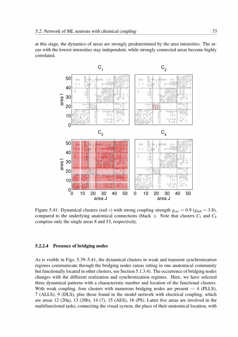
Figure 2.1: The representation of cat cortex in the form of the network: (a) binary matrixwith unspecified weights, (b) weighted matrix, where the different symbols represent differentconnection weights: 1 (black ◦ sparse), 2 (blue • intermediate) and 3 (red ∗ dense). The organi-zation of the system into four topological communities (functional subsystems, V, A, SM, FL)is indicated by the solid lines. See Chapter 3 for detailed description of the systems.

To characterize the structure and type of this network, we interprete and evaluate the maintopological properties relevant for our later analysis, taking a cortical area as a basic unit of anetwork.

• The most basic node characteristic is its degree k. For an area i, ki is the number ofconnections of the area i to the other areas in the network, i.e.,

ki = ∑j

A(i, j).

Incoming degree kin (afferent connections) and outgoing degree kout (efferent connec-tions) of an area can be differentiated.

• The intensity of a node Si, expresses the total strength of connections of the node (incom-ing Sin and outgoing Sout). It is the complete sum of the strength of all cortical fibers ofthe area:

Si = ∑j

W (i, j).

• Additionally, we also define reciprocity strength as the average weight of the links be-tween two nodes:

wi j ≡ (W (i, j)+W ( j, i))/(2wmax).


2wmax is the maximal bidirectional weight, e.g., in the case of the cat cortical network [99],the maximal weight is wmax = 3.

• The Matching Index MI between two nodes quantifies the number of their common neigh-bors. For comparative reasons it is convenient to normalize it by the the number of non-overlapping connections of these two nodes:

MI(i, j) =∑n

l=1 A(i, l)A( j, l)ki + k j−∑n

l=1 A(i, l)A( j, l).

Then MI(i, j) = 1 only if areas i and j receive input entirely from the same areas, andMI(i, j) = 0 if all inputs to i and j come from completely different areas. MI can beregarded as an estimation of the “functional similarity” of the nodes [51].

Based on the topology of the network and the structural properties, we distinguish four commontypes of networks — regular networks, small-world networks (SW), scale-free networks (SF)and random networks, see Fig. 2.2.

Figure 2.2: Different kinds of networks: (a) regular, (b) small-world, (c) scale-free and (d)random.

Roughly speaking, in regular networks, nodes usually have connections to a constant numberof nearest neighbors (Fig. 2.2(a)), whereas in random networks, the number and topology ofconnections between nodes are entirely random (Fig. 2.2(d)). Small-world (SW) topology rep-resents an intermediate structure between the random and regular one (Fig. 2.2(b)). Scale-free(SF) networks are characterized by the presence of a few hubs, i.e., nodes with a very highnumber of connections (Fig. 2.2(c)). Several authors have presented a general overview ofthese different kinds of networks, their network properties and the influence of such propertieson the network dynamics [19, 20, 84, 137].

SF and SW networks have especially been at the center of interest because of their commonoccurrence in nature, e.g., SF networks in functional brain networks [38] and SW networksin cortical networks [108, 110], in the neuronal network of Caenorhabiditis elegans [127] andalso in the functional networks [11]. We will pay special attention to the SW type of networks,originally proposed by Watts and Strogatz [127]. At the beginning, each unit of the networkconnects to a number ka of the nearest neighbors, alternatively specified by a connection densityparameter pring = ka/n. Later, links are rewired with a probability prew to a randomly selectednode, which introduces some long-range connections (‘shortcuts’). The parameters pring andprew are crucial for the selection of specific network character (regular, small-world or random),see [127].

2.3. Anatomical connectivity 9

Taking a neural network as an example of SW topology, the high average clustering coeffi-cient, expressing the large number of densely interconnected nodes, points out the existence ofclusters of neurons. The presence of a few shortcuts decreases the path length, i.e., the distancebetween two nodes i and j. The efficiency of neural communication within and between cell as-semblies is increased in networks with such properties. The spreading of the signal often leadsto synchronization of the dynamics of neurons [71, 72, 79, 47]. Such enhanced synchronizationhas also been confirmed by analytical studies [9, 88]. It has been argued that the evolution ofsystems into networks with small-world topology probably attempts to maximize the dynamicalcomplexity while minimizing wiring costs, i.e., cost-effective information processing [11].

The use of graph theory methods has revealed many basic characteristics of brain networks.Now, we introduce the general anatomical connectivity of the brain at different levels and itstopological properties.

2.3 Anatomical connectivity

Mammalian brain consists of a vast number of neurons that are interconnected in complexways [111]. In recent years, the network of anatomical links connecting various neural ele-ments, the connectome, has been the subject of intensive investigation. From numerous neu-rohistological studies, information about the morphology, location and connections of differenttypes of neuronal cells, microcircuits and anatomical areas has been collected and sorted. Thisdata plays an important role in creating a global image of the brain. The implementation ofsuch topological information in a large-scale neuronal model might help us to understand themechanisms of temporal and spatial spreading of brain activity.

2.3.1 Connectome

We describe the general structure of the mammalian connectome. Although the details of theneuronal network architecture are not fully known, several levels of cortical connectivity can bedefined [111].

Microscopic connectivity

In the human brain, approximately 1011 neurons are linked together by 1014−15 connec-tions, which corresponds to about 104 synapses per neuron on average. The network israther sparsely connected, with mainly local connectivity. Usually, each neuron makescontact to its closest neighbor only by one synapse or not at all [21, 95]. The interneu-ron connectivity patterns are very plastic, where changes are partially predetermined bygenetic constraints and later modified by factors like learning and nutrition. Since for along time it has not been possible to extract the microscale connectivity [18, 78, 104], theneural connections are commonly modelled as a graph. The architecture often takes the


form of a small-world network [71, 72, 79]. Other topologies are also considered, rang-ing from random [23, 59, 70] or globally coupled networks [15, 48, 53] to more realistictopologies reflecting spatial growth of the cortex [62].

Mesoscopic connectivity

The next level in the brain anatomical network is made up of cortical minicolumns. Acortical minicolumn, a narrow chain of neurons organized in the vertical direction acrosscortical layers II–VI, is considered to be a basic functional unit for processing informationin the brains of mammals [18, 94, 95]. Such local circuits consist of only 80–100 neuronswith an architecture more complex than just random or distance dependent connectionspatterns. Further, the minicolumn is deemed to be a basic building block of the com-plete connectome [25, 111]. A set of these functionally specialized and precisely rewiredsmall neuronal populations (usually 60–80 units) later gives rise to the cortical column(macrocolumn).

Macroscopic connectivity

In the cerebral cortex, neurons are also organized into numerous regions (areas) that dif-fer in cytoarchitecture and function. These areas, originally defined and listed by Brod-mann at the beginning of the 20th century, may be assumed to be basic elements at themacroscale [21]. The architecture and function of the areas, as well as the topology ofthe neuronal fiber connections linking different areas have been the subject of intensiveinvestigation. The anatomical network of visual cortex of monkey was described for thefirst time in 1991 by Felleman and van Essen [41]. More recently, cortical maps of otherspecies like rat [24] and cat [99, 100] have been published. Analysis of the obtained catanatomical cortical network revealed that the network possesses the small-world proper-ties [11, 108].

This detailed knowledge of the anatomical connectivity at the systems level of functional brainareas offers a good starting point to explore the undergoing dynamical processes.

2.3.2 Data extraction and databases

Anatomical information collected about the different levels of connectome has comes exclu-sively by invasive techniques (e.g., cutting axons and observing degeneration of cells, studyof postmortem brains, microinjection of dyes followed by autoradiographic imaging), meaningthat such information was mainly collected from animal studies. Several other factors like thehigh number of neurons, complex network topology or plasticity, make it impractical to extractthe precise connectivity at the anatomical microlevel. Newly developed imaging methods likeDiffusive Tensor Imaging may later help to obtain the details of human anatomical connectiv-ity [37].

All the extracted information about the anatomical connectivity of a number of animalspecies has been summarized and presented in various databases on several web sites. At the

2.4. Functional connectivity 11

mesoscopic scale the databases ‘Microcircuit’ [3] or ‘Wormatlas’ [6] offer insights into localcircuit connectivity. The database ‘Cocomac’ [2] contains connectivity maps of macroscopiccortical networks of macaque monkey, and ‘BrainMaps’ [1] maps the anatomical details ofdifferent animal species like domestic mouse, rat, cat, and several types of monkeys.

Our first task is to construct a topological model based on the known anatomical structure,which will provide the basis for modeling the dynamics of the system. We extract and inves-tigate functional networks to understand how the anatomical connectivity corresponds to thedynamics. In the next section, we describe what functional connectivity and functional net-works are and how we obtain them.

2.4 Functional connectivity

In the nervous system, processing and transmission of information are encoded in the form ofelectrical activity of individual neurons. The specific dynamical interactions between neuralelements and their statistical dependencies give rise to functional connectivity (FC) [33, 46].Being closely related to the underlying anatomical network [110], FC can be also estimatedat different levels of brain hierarchy, as described in Section 2.3. At the microscopic level,single neuron activity can be recorded with an intracellular microelectrode. The change ofmembrane voltage is expressed in the form of an action potential (AP). The dendritic synapticactivity of all neurons within a certain volume, a local field potential (LFP), can be measuredby a single extracellular electrode. Synchronized firing of neighboring neurons and summatedpostsynaptic potentials plus the AP of the active neuron give rise to the LFP. On this mesoscopiclevel, a large number of summed postsynaptic potentials from the surface of several squarecentimeters of cortex creates the EEG signal. This signal can be divided into several frequencybands, each related to a certain mental state. The EEG signal is complex, reflecting the stronglynonlinear neural dynamics and the intricate structure of the neuronal connections. The differenttypes of neurophysiological data can be obtained under different conditions, either in the basicresting state or while the brain is being stimulated, directly by strychnine injections [118] andby transcranial magnetic stimulation or indirectly in the form of mental tasks. In addition tothe records of the physiological signals, various neural models allow us to simulate neuronalactivity at different levels: action potentials, local field potentials or mean field activities ofwhole areas (see review [11]).

To obtain functional networks from data (physiological records or neural simulations), weproceed in two steps:

1. Evaluation of functional connectivityTo evaluate the FC between a pair of nodes or in a specific frequency band, we can use eitherlinear measures like cross-correlation, coherence and partial correlation [33, 98] or nonlin-ear measures like mutual information [110], generalized synchronization [13], synchronizationlikelihood [114, 116, 117], phase synchronization measures [90] or wavelet analysis [4].


It is difficult to decide which method allows us to extract functional connectivity most effec-tively [33]. Linear methods are more sensitive in the detection of the presence of neuronalcoupling and allow a fast characterization of data, but they are not able to capture nonlinear fea-tures. Nonlinear techniques better handle nonlinearity in the data, but they are computationallydemanding.

2. Extraction of functional networksThe pairwise FC between different regions forms a matrix from which the functional networkcan be extracted. A specific threshold is applied to this matrix and as a result an undirected graphis derived. If the value of the functional connectivity is larger than the threshold, a functionallink between two corresponding elements is established. Connections with the FC smaller thanthe threshold are removed. The final structure of the functional network, represented by a binarymatrix, depends on the number of regions included, the method chosen for the estimation of thefunctional connectivity and the thresholding rule [11].

Similar to anatomical networks, the topological properties of functional networks are thesubject of intensive investigation. There is evidence of SW properties in functional networks,based mainly on the presence of network characteristics such as short average path length andhigh clustering coefficient [4, 11, 12, 98]. Degree distribution offers additional informationabout the network: It might vary from the power law distribution of SF networks [38] to theexponential truncated power law somewhere between the exponential law of SW and powerlaw of SF networks. The resulting degree distribution guarantees the presence of a few hubs,but not as many as in SF networks. This property protects functional networks from attack andmakes the network more resilient [4, 115]. Recently, functional networks were also describedas fractal SW networks [12]. The small-world topology may play an important role in cognitiveprocesses, e.g., the change in cognitive ability associated with Alzheimer’s disease has beenlinked to the increased path length in the functional network [115].

2.5 Summary of the chapter

We have defined the three basic types of brain connectivity (anatomical, functional and effec-tive) and introduced the basics of graph theory, allowing us to represent the connectivity as anetwork and estimate the network properties. Details and properties of anatomical and func-tional connectivity were mentioned together with how to obtain and analyze the anatomical andphysiological data. At the end, we discussed the extraction of functional networks from thedata.

Chapter 3

Network topology of a large-scale model

After introducing the idea of the connectome in the previous chapter, we use the anatomicalinformation to build a hierarchical model of the brain. First, we describe the anatomical con-nectivity of the brain at the macroscale found in the cat cortical network. Each cortical area ismodeled by a subnetwork resembling basic features of the microscale connectivity. The result-ing system is then a network of networks.

3.1 Cat cortical network

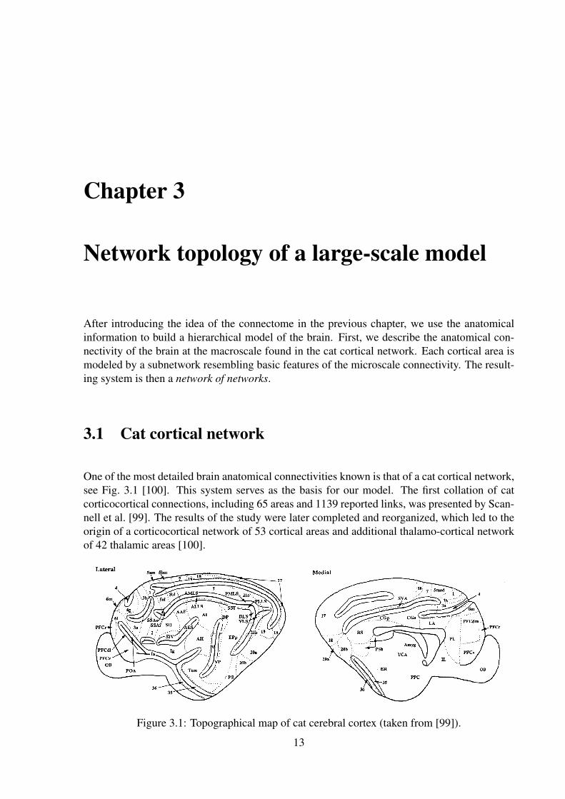
One of the most detailed brain anatomical connectivities known is that of a cat cortical network,see Fig. 3.1 [100]. This system serves as the basis for our model. The first collation of catcorticocortical connections, including 65 areas and 1139 reported links, was presented by Scan-nell et al. [99]. The results of the study were later completed and reorganized, which led to theorigin of a corticocortical network of 53 cortical areas and additional thalamo-cortical networkof 42 thalamic areas [100].

Figure 3.1: Topographical map of cat cerebral cortex (taken from [99]).

13

14 CHAPTER 3. Network topology of a large-scale model

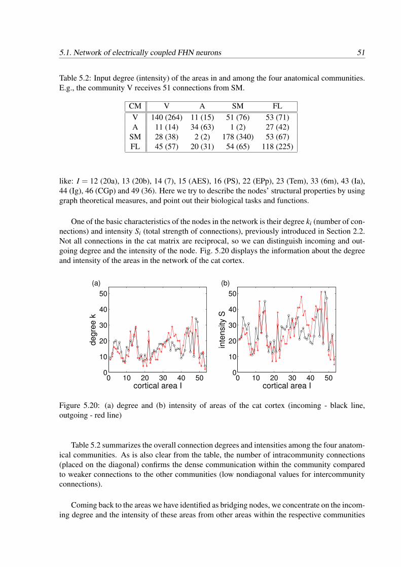
The corticocortical network of cat used in our model is composed of 53 highly reciprocallyinterconnected brain areas, see Fig. 3.2. The density of afferent and efferent axonal fibres isexpressed in three levels — ‘3’ for the densest bundles of fibres, ‘2’ for intermediate or unknowndensity and ‘1’ for the weakest connections. The value 0 characterizes absent or unknownconnections. These values convey more the ranks of the links than the absolute density of thefibres, in the sense that a ‘2’ is stronger than a ‘1’ but weaker than a ‘3’ [99, 100]. All together,there are around 830 connections in the corticocortical network with an average of 15 incominglinks and with average incoming strength of 26 per area.

Figure 3.2: Connectivity matrix representing connections between 53 cortical areas of cat brain.

In the network of cat cortical connections, four distinct subsystems can be identified. Threeof the subsystems — visual (V, 16 areas), auditory (A, 7 areas) and somato-motor (SM, 16areas) — involve regions participating in the processing of sensory information and executionof motoric function. The fourth subsystem — fronto-limbic (FL, 14 areas) — consists of variouscortical areas related to higher brain functions, like cognition and consciousness.

3.2. Hierarchical model — network of networks 15

The optimal placement of the cortical areas in the connectivity matrix was found by usinga nonmetric multidimensional scaling optimization method and already presented in the paperof Scannell et al. [99]. Such rearrangement of the areas led to the origin of these 4 subsystemsdescribed above. Later, several other methods based on network connectivity were applied toconfirm this optimal arrangement [49, 50, 100]. As a very relevant method we only mentionthe evolutionary optimization algorithm [49], where the number of connections between unitsof the cluster is maximized while inter-cluster connections are minimized. The resulting fourclusters agreed with the functional subsystems defined previously.

The corticocortical network has been subject to much detailed analysis based on graph the-ory (e.g., clustering coefficient, average path length, matching index and many other statisticalproperties) [108, 112] and theoretical neuroanatomy (e.g., segregation and integration) [107].Most of the studies focused on revealing the small-world nature of the structure of the cortex.The presence of clusters is one of the cortical characteristics. Parcellation of the cortex into ar-eas performing specialized functions corresponds to functional segregation. Cortical networksare also characterized by short path length between areas due to the few long-range connec-tions; this short path length allows efficient inter-areal communication. This corresponds to theidea of functional integration of information. The robustness of such networks [61] and theirhierarchical organization in the anatomical structure [31] have also been examined.

Because the properties of the structure of the cat cortex are well known, we chose the modelof cat cortical connectivity as the basis for our model of macroscopic anatomical connectivity.We distinguish two types of model, differing in their representation of the areas: (i) In one case,we extend the network structure and build a two-level network, i.e., a network of networks.Cortical areas appear in the model as subnetworks. The global dynamics of each area arisefrom the interaction and superposition of the dynamics of individual neurons. (ii) In the secondcase, the dynamics of the area are modeled directly by a population model and the structureof the network corresponds to the basic cat cortical matrix. Now we concentrate only on thetopology of the multilevel model.

3.2 Hierarchical model — network of networks

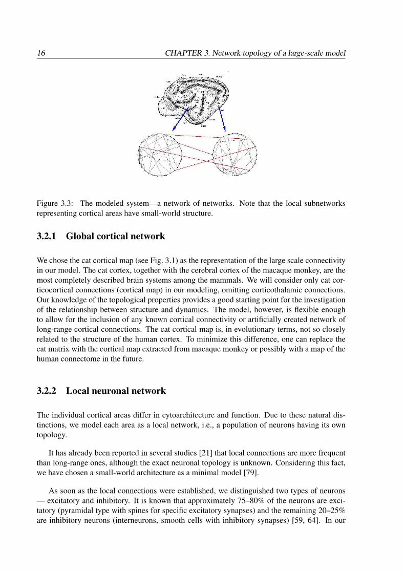
Due to the modular and hierarchical organization of the human connectome, simple modelsof individual cortical levels do not offer an appropriate insight into the complex dynamics oc-curring in such a complex topology. Thus, our model combines two cortical levels into oneframework. The higher level copies the known connectivity of real neuroanatomical data, par-ticularly the interconnectivity between 53 cat cortical areas [99, 100]. At the lower level, singlecortical areas are modeled by large neuronal ensembles. Implementation of these two layersgives rise to a specific topology—a network of networks, see Fig. 3.3. Some of the previousstudies have already dealt with such two level models (neuronal and areal) [109, 120]; however,none of them has introduced a detailed network topology in such an extension. As we will showin Chapter 5, this type of hierarchical network structure plays a crucial role in the uncoveringof dynamical properties of the system, see also [132, 138, 139]. In the following section, wedescribe the details of the topology of the model and discuss possible modifications.


Figure 3.3: The modeled system—a network of networks. Note that the local subnetworksrepresenting cortical areas have small-world structure.

3.2.1 Global cortical network

We chose the cat cortical map (see Fig. 3.1) as the representation of the large scale connectivityin our model. The cat cortex, together with the cerebral cortex of the macaque monkey, are themost completely described brain systems among the mammals. We will consider only cat cor-ticocortical connections (cortical map) in our modeling, omitting corticothalamic connections.Our knowledge of the topological properties provides a good starting point for the investigationof the relationship between structure and dynamics. The model, however, is flexible enoughto allow for the inclusion of any known cortical connectivity or artificially created network oflong-range cortical connections. The cat cortical map is, in evolutionary terms, not so closelyrelated to the structure of the human cortex. To minimize this difference, one can replace thecat matrix with the cortical map extracted from macaque monkey or possibly with a map of thehuman connectome in the future.

3.2.2 Local neuronal network

The individual cortical areas differ in cytoarchitecture and function. Due to these natural dis-tinctions, we model each area as a local network, i.e., a population of neurons having its owntopology.

It has already been reported in several studies [21] that local connections are more frequentthan long-range ones, although the exact neuronal topology is unknown. Considering this fact,we have chosen a small-world architecture as a minimal model [79].

As soon as the local connections were established, we distinguished two types of neurons— excitatory and inhibitory. It is known that approximately 75–80% of the neurons are exci-tatory (pyramidal type with spines for specific excitatory synapses) and the remaining 20–25%are inhibitory neurons (interneurons, smooth cells with inhibitory synapses) [59, 64]. In our

3.3. Summary of the chapter 17

simulations, we randomly selected the inhibitory neurons with a probability pinh = 0.25. Weconsidered all inter-areal links to be excitatory, since only pyramidal neurons are involved inthe long-range inter-areal connections. Inhibitory connections are involved in long-range con-nectivity only at the local level (within cortical columns [26]); due to the absence of a myelinlayer, they are not able to reach the speed necessary for signal transmission without significantdelay and loss of data [21]. Additionally, we also have to take into account signals coming fromother cortical areas (inter-areal links). If two areas are connected, only 5% of neurons withineach area receive or send signals to the other area. On average, up to 30–40% of neurons of onearea can be involved in communication with other areas [131].

We performed two studies which differed in the topology of long-range connections and theneuronal model together with the art of the neuronal coupling (discussed later in Chapter 4).We summarize the properties of the model topology for each case:

1. In the first part of our research, neurons communicate through the mean field signal,i.e., the selected 5% of neurons of one area get the mean field signal x = (1/n)∑n

i xi ofaveraged activity of n neurons from another linked area I. The coupling strengths forintra-areal coupling gint , i.e., the local excitatory and inhibitory synapses, have the samevalues. The inter-areal coupling strength gext differs from the local ones and both gint andgext play a key role in identifying different dynamical regimes.

2. In the second study, we randomly selected pext = 5% of the neurons of a ‘receiving’area to receive signals from pext = 5% of the neurons of a ‘sending’ area. Basically,we fix a total number of long-range connections between areas I and J as (n ∗ ka ∗ pext).The selected receiving neurons of area I receive numerous inputs from selected sendingexcitatory neurons of area J. We avoid multiple links, i.e., two neurons from differentareas can be connected only once. All established connections are directional. As wevary the coupling strength of the connections, here, for excitatory gexc and inhibitory ginhneurons, we obtain different dynamical regimes.

Table 3.1 offers an overview of all network parameters presented in the model of the networktopology.


Let us briefly summarize the structures of the model networks:

(i) In the first case, the system represents a network of networks, see Fig. 3.3. The upperlevel corresponds to the known anatomical connectivity map of 53 cat cortical areas. At thelower level, a single cortical area is modeled by a large neuronal population of excitatory andinhibitory neurons. The topology and the size of the local network can be adjusted by chang-ing the network parameters. We randomly choose 5% of the neurons to receive an input from


Parameter DescriptionN Number of areasn Number of neurons per areaka Number of connections per neuron within an area

prew Probability of rewiringpinh Ratio of inhibitory neuronspext Ratio of neurons of one area involved in long-range connectionsgint Non-normalized intra-areal (internal) strength of synapsesgext Non-normalized inter-areal (external) strength of synapsesgexc Non-normalized strength of excitatory synapsesginh Non-normalized strength of inhibitory synapses

Table 3.1: Parameters of the network—structure and connections

another connected cortical area, thus forgetting the layered structure of the cortical area and cor-responding topological details. Here, we consider two different topologies. In the first topology,the neurons receive an input in the form of average mean field signal of a sending area. We ex-amine dynamical regimes obtained by variation of inter-areal and intra-areal coupling strengths.In the second topology, 5% of the neurons of area J receive an input from 5% of the neurons(only excitatory) in connected area I.

(ii) The second investigated model of connected neural populations mimics the neural dy-namics on the macroscopic level. The number of neural populations and the connections be-tween them reflect the topology of the cat cortical network.

The following chapter deals with the dynamics occurring in all types of model topology.

Chapter 4

Modeling the global dynamics of theneuronal population

Up to now we have presented the brain as a complex network of interacting elements and mainlydiscussed the details of brain anatomy and connectivity at different levels (Chapter 2). Based onthis knowledge we have built a hierarchical model of brain, a network of networks (Chapter 3).In this chapter, we will concentrate on the neuronal dynamics and discuss the most relevantneuronal properties needed to model brain activity. The resulting dynamical patterns will beused to determine the functional networks. The linkage between the anatomical and functionalnetworks will be examined later (see Chapter 5, 6).

In attempt to model the global dynamics of the neuronal populations, usually measuredas EEG or LFP (Section 2.4), two main approaches are widely applied. The first approachsimulates a network of neurons, where the combination of the nontrivial connectivity of neuronsand the nonlinear behavior of the single neuron gives rise to complex dynamics. Following thisidea, we have constructed a model with a network of neurons representing a cortical area. Aset of neurons is connected according to a specific pattern of small-world network connectivityobserved commonly in nature. The second approach models the mean activity of the entireensemble of neurons. Such a population can represent a cortical column, or part of or theentire cortical area. The output signal is generated from sets of different types of neurons likepyramidal cells and excitatory and inhibitory neurons. Our model of neural mass mimics theactivity of a brain area. In this chapter, we present the details of both approaches.

4.1 Single neuron model

Neurons possess a complex morphology to handle the specific tasks of information transmis-sion and communication. The representation of neurons as a spatially extended unit with anintricate geometry would lead to a composite structural model of the neuron, computationallyvery expensive (see, e.g., [77]). Therefore, to simplify the neuronal model, neurons can bemodeled as dynamical systems with an emphasis on the various ionic currents that determine

19

20 CHAPTER 4. Modeling the global dynamics of the neuronal population

the neuronal excitability and response to stimuli. The neuronal response can be captured by asimple threshold or excitable model and the dynamics of the neurons can be described by twovariables V and W :

Vi = f (Vi, Ibias)+ Isyni (t)+ Iext

i (t) (4.1)Wi = h(Wi) (4.2)

The dynamics of the fast variable V , imitating the membrane potential, are predetermined bya function f of two parameters: the membrane potential V and the basic current Ibias, whichflows into the neuron and sets up the neuronal excitability. Moreover, the membrane potentialV is modified by the total synaptic current Isyn coming from other connected neurons and theexternal current Iext , representing perturbations from lower brain parts. The dynamics of slowrecovery variable W , modeled by a function h, account for the activity of various ion channels.

Excitable neurons can be categorized into two classes based on their excitability and theirresponse to an input [55, 57, 71]. Class 1 excitability contains those neurons able to encodethe strength of the input into their firing activity, even with a weak input (Fig. 4.1(a)). Suchneurons undergo a saddle-node bifurcation, with firing frequencies ranging from 2 to 200 Hz.Typical cells with such activity are pyramidal neurons, representing the majority of the corticalunits. Class 2 excitability neurons do not respond to the input so flexibly and cannot fire atlow frequencies (Fig. 4.1(b)). Their dynamics are characterized by a Hopf bifurcation, withan on/off behavior: Either the neuron does not fire, or it fires at a high frequency (like 40Hz) [55, 71, 113].

30 40 50 60 70 80 90 1000

10

20

30

40

input (mV)

fre

qu

en

cy (

Hz)

(a)

70 80 90 100 110 120 130 140 150 1600

10

20

30

input (mV)

fre

qu

en

cy (

Hz)

(b)

Figure 4.1: Dependence of the firing rate on the intensity of the applied current (Morris-Lecarmodel adopted from [123]): (a) Class 1 excitability, (b) Class 2 excitability.

From a variety of point spike models, e.g., Integrate-and-fire model, Hindmarsh–Rose model,Izhikevich model (see [55, 92]), we chose two different types of model. In addition to the detailsof the neuronal models, the properties of the neuronal coupling and stimulation are describedand discussed in the following section.

4.1. Single neuron model 21

4.1.1 Model of a single neuron

We introduce two neuronal models that capture the main features of neuronal dynamics likespiking, resting state, etc. The first model, the FitzHugh-Nagumo model, is an excellent exam-ple of an excitable system of class 2. This simple model of a relaxation oscillator is commonlyused in neuroscience but has also various other applications, like in the kinetics of chemical re-actions, or in solid state physics [89]. The second model is the Morris-Lecar model (ML), whichis a canonical prototype for different classes of neuronal membranes. With a slight variation ofthe parameters, the ML model is able to exhibit both class 1 and class 2 neuronal dynamics.

4.1.1.1 FitzHugh-Nagumo model

FitzHugh proposed a model in 1961 [42], which was originally called the Bonhoeffer-van derPol model. His main aim was to investigate basic dynamic interrelations between state variablesof a cell membrane. At the same time, Nagumo constructed an electronic circuit exhibiting thesame properties as the FitzHugh model [58] and now the model is known as the FitzHugh-Nagumo model (FHN). We adopted the version of the FHN introduced by Pikovsky et al. [89]and later used in numerous studies [52, 101, 135, 140]:

εxi = xi− x3i

3− yi, (4.3)

yi = xi + ai. (4.4)

The fast excitable variable x represents the membrane potential; its cubic nonlinearity allowsregenerative self-excitation via positive feedback (Eq. 4.3). The slow recovery variable y isresponsible for accommodation and refractory behavior; its linear dynamics produce slowernegative feedback (Eq. 4.4).

The small value of the time scale parameter (ε = 0.01) allows the separation of the motion ofthe two variables x and y. The parameter a is a bifurcation parameter responsible for excitatoryproperties of the system, where |a| > 1 corresponds to a stable fixed point and |a| < 1 to alimit cycle. We set ai ∈ (1.05,1.15), and thus the neurons are in the excitable state, closeto the bifurcation threshold. A small perturbation of such a state switches the activity to theoscillatory regime (see Fig. 4.2). We use the FHN model to describe the dynamics of individualneurons mainly because of its simplicity and biological plausibility [55]. This model is not aquantitative representation of a neuron, but it rather concentrates on the qualitative propertiesof neuron, modeling the dynamics of class 2 excitability. Even though it does not capture allfeatures of the neuronal dynamics, the model still provides a signal similar to simple neuronalactivity with properties like resting state and neuronal firing.

4.1.1.2 Morris-Lecar model

The second neuronal model we used in our simulations was the Morris-Lecar model, consideredto be a canonical prototype for two classes of neuronal membranes. The Morris-Lecar model


10 15 20 25

−2

−1

0

1

2

time

x

(a)

−2 −1 0 1 2−1

−0.5

0

0.5

1

x

y

(b)

Figure 4.2: (a) FHN neuron in oscillatory state. (b) Phase portrait for FHN neuron.

was introduced by Morris and Lecar in 1981 during a series of studies of the excitability ofthe barnacle giant muscle fiber [93]. The dynamics of the cell membrane was determined bytransmembranar currents — the voltage-gated Ca2+ current, the voltage-gated delayed-rectifierK+ current and the leak current. The original third-order system of nonlinear equations denotesthe voltage V and the activity of the depolarizing Ca2+ and hyperpolarizing K+ channels. Dueto the fact that calcium channels respond to V very rapidly, instantaneous activation is assumedand the model can be reduced to the two-dimensional form (Eqs. 4.5– 4.6) [93]:

CV = I−gL(V −VL)−gKW (V −VK)−gCaMinf(V )(V −VCa), (4.5)W = λ(V )(Winf(V )−W ), (4.6)

where

Minf(V ) = 0.5[

1 + tanh(

V −V1

V2

)], (4.7)

Winf(V ) = 0.5[

1 + tanh(

V −V3

V4

)], (4.8)

λ(V ) = φcosh(

V −V3

2V4

). (4.9)

The activity of Ca2+ channels is included in the membrane voltage V , whereas the variable Wrepresents the fraction of the open K+ channels. C stands for the membrane capacitance perunit area and φ is a temperature-like scale factor, a decay rate of W , here considered to be aconstant. ga are the conductances and Va resting potentials for calcium, potassium and leakchannels (a = Ca,K,L). Each neuron receives a constant input I, which determines the state ofthe neuron — either the resting (excitable) state, when the input is smaller than a critical biascurrent (I < Ic), or the oscillatory state, when the input is above the threshold (I > Ic). Fig. 4.3shows the phase portrait of the oscillatory regime with corresponding voltage dynamics. Weset Ii ∈ (37.0,38.0), when neurons are in the excitable state, close to the bifurcation threshold.Oscillations are achieved after perturbation of dynamics either through noise or signals fromother neurons. All other parameter values were taken from Tsumoto [123] (Tab. 4.1) to modelthe dynamics of a single class 1 excitability neuron. The ML model is special since it can, with


100 150 200 250 300−80

−40

0

40

80

time (ms)

V (

mV

)

(a)

−50 0 50

0

0.1

0.2

0.3

0.4

V

W

(b)

Figure 4.3: (a) Oscillatory dynamics of a ML neuron, class 1 excitability. (b) Phase portrait forML neuron.

small change of parameters, also exhibit dynamical features of class 2 excitability (Fig 4.1(b)).Tsumoto has also shown that the parameters gCa, φ, V3 and V4 are crucial in the switching of thedynamics. When Iext is relatively small, the simple change of the value of V3 from 12 to 2 mVcauses the dynamics to switch from class 1 to class 2 excitability, see [8, 123]. Thus, this modelis suitable for modeling of heterogeneous groups of neurons. The same model with slightlydifferent parameters was also used in our large-scale simulations of a neural network [10].

gL[µS/cm2] 2 VL[mV] -60 V1[mV] -1.2gK[µS/cm2] 8 VK[mV] -80 V2[mV] 18gCa[µS/cm2] 4 VCa[mV] 120 V3[mV] 12

φ[s−1] 1.015.0 I[mA] 38.5 V4[mV] 17.4

Table 4.1: Parameters of ML model of neuron (adopted from Tsumoto et al. [123]).

4.1.2 Factors influencing dynamics of a neuron

Previously described neuronal models can truly mimic the dynamics of a single neuron undercertain conditions (in steady or oscillatory state, under stimulus). In the modeling of simpleneuronal systems, two additional features are of great importance — (i) the presence of noisein the system, which determines the dynamical state of the neuron (oscillation) and (ii) the artof coupling of the basic elements, i.e., neurons or areas, expressing the influence of one systemupon another one.

4.1.2.1 Role of noise in neural system

In the living brain, neurons in the normal state usually do not exhibit strong activity. Accordingto some estimates, they are silent 99% of the time, just sitting below the critical threshold and


being ready to fire [44]. In our models, the neurons are also initially set to the excitable state(parameters a in the FHN model and I in the ML model are below the critical threshold).

We add Gaussian white noise 〈ξi(t)ξ j(t − τ)〉 = δi jδ(τ) to mimic the intrinsic stochasticcharacter of neuronal dynamics, caused by stochastic processes like synaptic transmission orspontaneous release of neurotransmitter into the synaptic cleft [28, 113]. The tunable parameterD (see later Eqs. 5.2, 5.13) scales the intensity of this random input. To obtain the natural firingrate of individual neurons (1–3 Hz), we can vary the intensity D until the expected firing rate isreached.

In some work, neurons are stimulated by multiple inputs of Poissonian noise to simulate externalinfluences, e.g., from subcortical areas [23, 44, 56, 70]. In the study of a large-scale neuronalsystem [10, 133], we implemented both Gaussian and Poissonian noise.

4.1.2.2 Synaptic coupling between cortical neurons

1011 neurons in the human brain form a sparse network, where an average neuron forms about103− 104 synaptic connections. There are two distinct types of synaptic coupling: electricaland chemical [64].

Electrical coupling (linear) appears only locally through the close contact of the cell membraneof the neurons (3.5 nm) without the presence of synaptic neurotransmitter. The informa-tion about the change of membrane potential of one neuron is transmitted directly as acurrent flowing through ion channels called gap junctions. The simplest linear couplingbetween two neurons i and j would take the form

xi = f (xi)+ g(x j− xi),

where g is a strength of the connection [54]. Such diffusive coupling is not the mosttypical case in the mammalian cortex (occurs mainly in interneurons), but we use it in onepart of our study to simplify that stage of our simulation (see later Section 5.1, Eq. 5.1).

Chemical connections (nonlinear) represent the majority of connections between neurons inthe neocortex. The principle of signal transmission is based on the release of chemicalmessengers from the depolarized presynaptic neuron, which consequently bind to the re-ceptors of the postsynaptic neuron. This causes the flow of ions in the postsynaptic neuronleading to the polarization of the membrane. Depending on the type of the receptor, wecan distinguish excitatory or inhibitory neurons, which occur in the ratio of about 3:1 (im-plemented in the model as pinh = 0.25). Excitatory neurons enhance the spreading of theaction potential and excite the postsynaptic neuron. Inhibitory neurons inhibit neuronalactivity and act to hyperpolarize the postsynaptic membrane.

Several models of chemical coupling are widely used, varying from a simple one expressed bya ‘threshold’ function [54] to more complex ones described by sets of equations [48, 64, 71,


Parameter Excitatory InhibitoryEs (mV) 0 -80αs (ms−1 mM−1) 2 0.5βs (ms−1) 1 0.1

Table 4.2: Parameters of the synaptic coupling for excitatory and inhibitory neurons.

72]. In the second part of our study (Section 5.2), we adopted the model of chemical couplingdescribed by Lago-Fernandez [71], which will be now discussed in detail. The input from thesynapses to the neuron Isyn

i (see Eq. (5.13)) is added to the fast voltage variable V . This synapticterm represents the total synaptic current to the ith cell, i.e., the sum of signals (spikes) fromall pre-synaptic neurons, k = 1, . . . ,ntotal . ntotal is the number of afferent synaptic connectionsfrom all local and extra-areal neurons to neuron i:

Isyni (t) =

ntotal

∑k

gi jr j[Vi(t)−Es]. (4.10)

The response from an individual synapse is modeled by the difference between the membranepotential of the postsynaptic neuron Vi and the reversal potential Es (see a similar approachin [70, 71, 72]). Es stands for Eexc or Einh depending on whether the presynaptic neuron isexcitatory or inhibitory. The parameter gi j is the maximum conductance per unit area, whichdetermines the connectivity and coupling strength between the postsynaptic i and presynaptic jneurons. In the case of disconnected neurons, we have gi j = 0; gi j > 0 indicates the presenceof excitatory links and gi j < 0 the presence of inhibitory ones.

The amount of released neurotransmitter into the synaptic cleft determines the fraction of theopen channels r in the postsynaptic neuron:

r j = αsx j(1− r j)−βsr j, (4.11)

where αs and βs are time-dependent rise and decay constants, with s symbolizing whether theneurons are excitatory or inhibitory. The corresponding values of the parameters for synapticcoupling are summarized in Table 4.2. Neurotransmitter concentration x j is typically modelledas a square pulse, see Destexhe et al. [36]. To make the change in the concentration smoother,the limits in the transmitter concentration at a constant presynaptic potential Vpre are expressedby the function f (Vpre):

x j = α( f (Vpre)− x j), (4.12)

f (Vpre) =σ

1 + exp(−(Vpre−θ)/T ), (4.13)

where α = 5 ms−1, σ = 2.84 mM, θ = 2 mV, T = 5 mV [72].

With this model of the chemical synapses, the coupling gains nonlinear terms and the dynamicsof the network become even more complex.


4.1.2.3 Other neuronal properties

There are several other neuronal properties modulating neuronal reaction and activity propaga-tion within the network that we did not consider in our research. One of them is the spreading ofthe signal in the network, influenced by transduction delays tdel . Delays typically vary between0.1–20 ms [68] and depend on the neuronal morphology [40]. Further, the strength of the synap-tic connection is plastic; the mechanism of spike-timing-dependent plasticity (STDP) [17, 106]modifies the weight of connection between the neurons in dependence on the exact time differ-ence between postsynaptic ti and presynaptic t j spike arrival, see [56, 106].

These properties also play a significant role in the dynamics of the brain, but becauseof the added model complexity, high computational costs would incurred when adding suchproperties. Example of their implementation in a large-scale model of brain can be foundin [10, 14, 133].

As one can see, the modeling of a network of coupled neurons with many biological detailsof neuronal dynamics and coupling can be quite complex. A neural mass model offers analternative way to model the dynamics of the neuronal population; we discuss its properties inthe next section.

4.2 Neural mass model

EEG measurements record the mean activity of a population of neurons in the brain, oftenexhibiting rhythmic oscillations within well-defined frequency bands. A neural mass model de-scribes the activity of such populations of cortical neurons and can reproduce the main featuresof EEG dynamics.

The first models of neuronal dynamics on the macroscopic scale appeared in the early1970s [32, 43]. Lopes da Silva constructed a simple lumped parameter model of two popu-lations of neurons (excitatory and inhibitory) coupled with negative feedback, generating analpha rhythm [32]. Later, Jansen et al. [16] extended this model by modeling three subgroups:excitatory pyramidal cells and excitatory and inhibitory interneurons, adding also nonlinearterms to the equations. Wendling et al. [128, 129] concentrated in their works on modelingdifferent patterns of EEG signals observed in epileptic patients. An improved version of theprevious two models [16, 32] was able to generate EEG signals from multiple coupled neuronalpopulations in various frequency bands. The next variant of the model contained four neuronalsubsets; the inhibitory neurons were further distinguished with fast or slow kinetics [128]. Re-cently, David mimicked EEG/MEG dynamics using hierarchically coupled models of neuronalpopulations [34, 35] and Ursino et al. [124] presented a model with parallel implementation ofthree different populations reproducing different rhythms of brain activity.

In our work, we use the neural mass model and parameters presented in [129], see Fig. 4.4for a graphical representation of the model.


Figure 4.4: Neural mass model, adopted from [16]. Here, y0 stands for vp, y1 for ve and y2 forvi, p(t) is the noise input, as shown later in Chapter 6.

Here, a population of neurons contains two subpopulations: subset 1 consists of pyramidalcells receiving excitatory or inhibitory feedback from subset 2. Subset 2 is composed of localinterneurons receiving excitatory inputs. This model describes the evolution of the macroscopicvariables, i.e., average postsynaptic membrane potentials vp for pyramidal cells, and ve, vi forthe excitatory and inhibitory interneurons, respectively. A static nonlinear sigmoid functionf (v) = 2e0/(1+er(v0−v)) converts the average membrane potential into an average pulse densityof action potentials. v0 is the postsynaptic potential corresponding to a firing rate of e0, and r isthe steepness of the activation. The dynamical equations for a single population are:

vpI = Aa f (ve

I − viI)−2avp

I −a2vpI , (4.14)

viI = BbC4 f (C3vp

I )−2bviI−b2vi

I, (4.15)

veI = AaC2 f (C1vp

I )−2aveI −a2ve

I , (4.16)

where vpI , vi

I and veI are the postsynaptic membrane potentials of the area I. A detailed interpre-

tation and the standard parameter values of this model are presented in Table 4.3. The details ofthe dynamics of multiple coupled populations and their relationship to the underlying anatomywill be discussed in the next chapter (Chapter 6).


We have presented two different approaches to model the dynamics of neural ensemble. (i) Thefirst approach considers the single neuron to be the basic element of the population. Connect-ing numerous neurons gives rise to the population dynamics representing a cortical area in our


Parameter Value InterpretationA 3.25 mV average E synaptic gainB 22 mV average I synaptic gain1/a 100 s−1 dendritic average time constant in the feedback E loop1/b 50 s−1 aver. time constant in the feedback I loopC1 C=135 aver. number of synaptic contacts in the E feedback loop,C2 0.8 CC3 0.25 C aver. number of synaptic contacts in the I feedback loopC4 0.25 Cv0, e0, r (mV) parameters of the nonlinear asymmetric sigmoid function

Table 4.3: Model parameters, their values and interpretation (E = excitatory, I = inhibitory),adopted from [128, 129].

study. We have shown two point models with different excitability classes — the FitzHugh-Nagumo (FHN) and Morris-Lecar (ML) models. The FHN model captures the basic features ofthe neuronal dynamics and has class 1 excitability. It is a rather simple model, computationallyinexpensive and thus suitable for the modeling of large networks. We coupled the set of FHNneurons by simple electrical coupling. However, in reality, around 70% of neurons are pyrami-dal cells with class 2 excitability and the neuronal coupling is mediated by chemical transmitterwith complex dynamics. The ML model is suitable for simulations of such properties and more-over by the change of only a few variables, it can switch its behavior to class 1 excitability. Theneuronal model composed of ML neurons is coupled by chemical synapses. These featuresincrease the biological relevance of the model but also the computational difficulties. (ii) Thesecond approach uses a neural mass model to imitate the dynamics of neuronal ensembles. Thismodel substitutes the modeling of the dynamics of the network of neurons representing onecortical area.

The general dynamics generated by these diverse models will be presented and discussed inthe next chapters (Chapter 5 and 6).

Chapter 5

Hierarchical model of cat cortex

We investigated the behavior of the multilevel model with two different types of neuronal dy-namics. In the first case, the neurons represented by FitzHugh-Nagumo model are electricallycoupled and the areas communicate through the mean field signal. The second case employsthe neuronal model of Morris-Lecar coupled through chemical synapses with neuron-to-neuroncommunication between areas. This synaptic coupling has a nonlinear character, which makesthe neuronal dynamics more complex. Here, we will describe the main features of the dynam-ics induced by both models, reveal the hierarchy of functional networks, that is similar to thestructure of the underlying anatomical network, and show the presence of functional clusters.We will also discuss the reasons for such behavior and its biological relevance.

5.1 Network of electrically coupled FHN neurons

5.1.1 General dynamics of the model

As we have already introduced in Chapter 3, in our model of the cat cortex the neurons standfor the basic elements of the two-level hierarchical network. The general set of equations of thewhole system in the case of FHN neurons takes the form:

εxI,i = fFHN(xI,i,yI,i)+gint

ka

n

∑j

MLI (i, j)(xI, j− xI,i)

+gext

〈w〉N

∑J

MC(I,J)LI,J(i)(xJ− xI,i), (5.1)

yI,i = hFHN(xI,i,yI,i)+ DξI,i(t), (5.2)

where x is the membrane potential modelled by a particular function f , see Eq. 4.3. It is alsomodulated by the input from neighboring neurons from the local network (coupling represented

29

30 CHAPTER 5. Hierarchical model of cat cortex

by local connectivity matrix ML) and input from remote neurons from other areas (couplingrepresented by cat cortex connectivity matrix MC). Here, we set up that the connected areascommunicate through their mean field activity x = (1/n)∑n

j x j. The label LI,J(i) is 1 if neuroni is among the 5% within area I receiving the mean field signal from area J, otherwise, LI,J(i)is 0 [131]. In spite of the fact that diffusive electrical coupling occurs only in a minority ofthe neuronal synapses, we use it in our model in order to simplify the connections between theneurons. Once the dynamical principles of the simpler model are understood, we will use morerealistic chemical coupling (see Section 5.2). To each neuron, we add the weak Gaussian whitenoise ξ with intensity D = 0.03 to the slower variable to simulate the natural perturbation of thedynamics (Eqs. 4.4, 5.2). We tune the parameter D until we do not obtain signal for one area,similar to the background irregular neuronal activity of a silent neuron. Such signal correspondsto the average neuronal activity of the set of coupled neurons in the resting state with occasionalbursts of activity, similar to EEG signal at resting state [87]. The coupling properties and therole of the noise in the system have been described in details in Section 4.1.2. We would liketo emphasize that the Euler method, used for numerical integration, is appropriate due to thestochastic term ξ in the system. The model is coded in the Fortran 90 programming language.

Parameter study

We simulate the above system of Eqs. 5.1–5.2, the network of networks of FHN neurons, upto time t = 2000. A time step ∆t = 0.001 is applied which is sufficiently small for the stochasticdynamics. To keep the simulation time reasonable, we fix the small-world subnetworks to haven = 200 neurons, ka = 12 neighboring links, and a probability of rewiring of prew = 0.3. Despitethe relatively large value of the rewiring probability we still obtain the small-world properties ofthe network. We select n = 200 as large enough to exclude the system size effects by checkingthe amplitudes (standard deviation) of the mean field x of the individual SWNs without externalcoupling (gext = 0). We also ran the whole system with other values of prew and n, and twodifferent settings of the parameters gint and gext that select the two main dynamical regimes (seelater in this section); the obtained results confirm the robustness of the dynamics to changes inthe local network topology.

Except for the noise intensity parameter D, here fixed to a constant level, the dynamics of thesystem are controlled only by the internal gint and external gext coupling strengths. We explorethe parameter space for gint and gext and investigate how the dynamics of the individual areasare synchronized. To evaluate the degree of synchronization among these stochastic signals, asimple but effective linear measure, the Pearson correlation coefficient r, is used. We computethis correlation coefficient between the the mean field activities xI of the areas using long timeseries after the transient, namely,

r(I,J) =〈xI xJ〉−〈xI〉〈xJ〉

σ(xI)σ(xJ), (5.3)

where 〈·〉 denotes averaging over time. Further, the average correlation coefficient over all theN(N−1) pairs of areas,

R = [1/N(N−1)]N

∑I 6=J

r(I,J), (5.4)

5.1. Network of electrically coupled FHN neurons 31

quantifies the overall level of synchronization in the whole network system.

In the local SWNs, the spiking dynamics and the synchronization of the neurons are mainlycontrolled by the internal coupling gint [135] that determines the mutual excitation between anypair of neurons. For small gint , a neuron is primarily activated by the noise, and not usually bythe spiking activity of its neighbors. Thus, we observe irregular spiking patterns for individualneurons. The mean field x is characterized by some clear deviations from the baseline, demon-strating the weak synchronization within and also between the subnetworks (Fig. 5.1(a)). Suchmean field activity of individual areas can be regarded as an analogue of the EEG signal [87].The weak synchronization between such signals of the different areas is also shown by a smallaverage correlation coefficient R (Fig. 5.4(a)). Increase of the coupling strength gint leads to theincrease of the synchronization between the neurons within the local subnetworks, manifestedby the presence of some apparent peaks in x (Fig. 5.1(b)). With large enough gint , the neu-rons are mutually excited, achieving both strongly synchronized and regular spiking behavior(Fig. 5.1(c)), indicating an almost global synchronization of the network.

15.0 15.1 15.2 15.3

−1.2

−1

−0.8

−0.6

time

mean fie

ld

(a)

15.0 15.1 15.2 15.3

time

(b)

15.0 15.1 15.2 15.3−2

−1

0

1

2

time

(c)

Figure 5.1: Typical time series of the mean field dynamics x of one area with different couplingstrengths (gint = gext): (a) gint = 0.06, (b) gint = 0.082 and (c) gint = 0.12. Notice the differentscales on the vertical axes.

Additionally to the main driving parameter of the network, gint , the external coupling gexthas also an effect on the synchronization of the neurons in the local network (amplitudes of x),as well as on the control of the synchronization between the areas. For small gint , the infrequentand irregular spiking activity of one area does not very much affect the behavior of the otherconnected areas. The correlations between the areas are not strong even for significantly largegext (r ≤ 0.1). This is mainly due to the fact that only 5% of the neurons receive signals fromanother connected area [131]. For intermediate gint (e.g., 0.080± 0.003), the effect of gext onthe total synchronization of the network is clearly visible (Fig. 5.3(a)). With large values of gint ,the frequent and regular spiking activity of one area has significant effects on the spike timingof the other connected areas. The whole network exhibits strong synchronization even forrelatively small gext . Fig. 5.2 illustrates the typical behavior in three regimes. We can observesome weakly synchronized activities among certain areas in Fig. 5.2(a), the slight increase inthe amplitude of the spikes in the transient regime in Fig. 5.2(b) and the high spiking amplitudewith some temporal interruption of the strong synchronization in some areas in Fig. 5.2(c).


The behavior of the system in the weak synchronization regime, i.e., the infrequent spik-ing of neurons and the irregular activity of the weakly synchronized brain areas, is biologicalplausible and comparable to normal brain activity. On the other hand, the regular spiking char-acteristically found in the strong synchronization regime, both in the dynamics of single neuronsand brain areas, could correspond to pathological states such as epileptic seizure [70, 74].

area I

tim

e

(a)

10 20 30 40 50

15.1

15.2

15.3

15.4

15.5

−1.2

−1

−0.8

−0.6

area I

(b)

10 20 30 40 50

−1.5

−1

−0.5

0

area I

(c)

10 20 30 40 50

−1.5

−1

−0.5

0

0.5

1

1.5

Figure 5.2: Spatio-temporal patterns of the mean activity xI at different coupling strengths(gint = gext): (a) gint = 0.06 (b) gint = 0.082 and (c) gint = 0.12. Note the different scales in thecolorbars.

Further, we focus on the correlation of the areas, R, at various coupling strengths. A plot ofR as a function of the coupling strengths gint and gext is shown in Fig. 5.3(a). We have averagedthe results over 10 realizations of the initial conditions and the topology of the SW subnetworksfor each set of the parameters. As already discussed, an increase of the coupling strengths gintleads to stronger interaction of the neurons and to a rapid growth of their synchronous activitywithin and across areas for non-vanishing gext (Fig. 5.3(b)).

The correlation matrices r(I,J) for the three regimes are shown in Fig. 5.4. Although theaverage levels of synchronization R are very different, the correlation patterns display somedynamical clusters, where a dynamical (functional) cluster is defined as a group of brain ar-eas communicating much more strongly within this set than with the areas in the rest of thebrain [122] (see also the definition of functional connectivity in Section 2.1). In the weak syn-chronization regime with the correlation r ∈ [0,0.1], four dynamical clusters are visible thatresemble the underlying anatomical structure (Fig. 5.4(a)). The transient regime, correlationsin the range [0,0.4], captures the reorganization of areas into three dynamical clusters. Fig-ure 5.4(b) does not clearly show these three clusters, but such separation is later revealed byclustering analysis. Finally, in the strong synchronization regime with r ∈ [0.6,1.0], we canobserve two dominant clusters (Fig. 5.4(c)). These clusters are also evidently present in thespatio-temporal patterns in Fig. 5.2(c).

The characterization of these dynamical clusters and their precise relation to the underlyinganatomical communities was our main concern and will be presented in the next section.


gint

gext

(a)

0.03 0.09 0.15 0.21

0.03

0.06

0.09

0.12

0.15

0.18

0.21 0.1

0.2

0.3

0.4

0.5

0.6

0.7

0.8

0.9

0.05 0.1 0.15

10−2

10−1

100

gint

R

(b)

Figure 5.3: (a) Dependence of the average correlation coefficient R on the internal and externalcoupling strength gint and gext . (b) The effect of the internal coupling strength gint on the globalcorrelation R (with fixed gext = 0.06).

area J

are

a I

(a)

0 10 20 30 40 50

50

40

30

20

10

00

0.02

0.04

0.06

area J

(b)

0 10 20 30 40 500

0.1

0.2

0.3

0.4

area J

(c)

0 10 20 30 40 500.6

0.7

0.8

0.9

Figure 5.4: Correlation matrices r(I,J) corresponding to the spatio-temporal patterns inFig. 5.2. (a) gint = 0.06, (b) gint = 0.082 and (c) gint = 0.12. In all cases r(I, I) = 1.0. Note alsothe different scales in the colorbars.


5.1.2 Revealing the network hierarchy

Visual inspection of the correlation matrix r(I,J) shows a good match between the dynami-cal clusters in the weak synchronization regime and the underlying anatomical communities.Fig. 5.4(a) suggests that the dynamics of the present multilevel model has a nontrivial orga-nization and an intriguing relationship with the network topology. To better characterize thisrelationship, let us now concentrate on the distribution of the correlation under four conditions.First, we are interested in the distribution of r(I,J) among all pairs of areas: this exhibits aGaussian peak around zero, but with a long tail toward large positive values. The significanceof these large values is confirmed by comparison to correlation r(I,J) of surrogate data obtainedby random shuffling of the original time series xI . Further, based on the argument of the signalpropagation, we distinguish three types of connections between any pair of areas in the network:

• reciprocal connections (P2)

• uni-directional connections (P1)

• non-connections (P0)

0 0.1 0.20

0.1

0.2

0.3

r(I,J)

pro

ba

bili

ty

(a)

0 0.2 0.40

0.1

0.2

0.3

0.4

r(I,J)

(b)

0.6 0.8 10

0.1

0.2

0.3

0.4

r(I,J)

(c)

Figure 5.5: Distribution of the correlation r(I,J) (a) g = 0.07, (b) g = 0.082 and (c) g = 0.12for all nodes (black line), P2 (blue line), P1 (red line) and P0 (green line). The dashed-dottedline denotes the results for the surrogate data.

The distributions of r(I,J) for these three cases display well-separated peaks in the weakcoupling regime (Fig. 5.5(a)). The dynamics of the cortical areas connected by reciprocalanatomical links, P2, tends to be more strongly correlated than the dynamics of areas con-nected by one link, P1. Compared to the surrogate data, almost all the P2 pairs have significantcorrelations. With strong coupling (e.g., g≥ 0.09), the excitation propagates through the wholenetwork and the separation of distributions of correlations is no longer so clearly pronounced(Fig. 5.5(c)). Generally, with increase of the reciprocity and the strength of the connection, weobserve a shift of the peak of the distribution towards larger correlation values.


The weak coupling regime is biologically more realistic with a low frequency and irregularspiking behavior. Here, the propagation of the signal between connected areas is mediated bysynchronized activities (peaks in x). A temporal correlation is most likely established when thereceivers produce similar synchronized activities by this input, or when two areas are excitedby correlated signals from common neighbors. Due to the weak coupling and the existence ofsubnetworks, such a synchronized response does not always occur, thus a local signal (excita-tion) does not propagate through the whole network. As a result, the correlation patterns areclosely related to the network topology, although the values are relatively small due to infre-quent signal propagation. With strong coupling, the signal can propagate through the wholenetwork strongly influencing also distant areas and leading to high correlation among areas, ascorresponds to pathological situations, such as epileptic seizures [70].

5.1.2.1 Functional connectivity

To characterize the obtained dynamical networks, their topology and relation to the underlyinganatomy, we use several graph theoretical measures described previously in Section 2.2. First,link reciprocity and its impact on the correlation of the activity between areas is considered.Figure 5.5 displays larger values of correlation between areas that are anatomically connectedby reciprocal links. Furthermore, correlation is also expected to depend on the connectionweights. We define the reciprocal weight, wIJ , as the normalized sum of the link strengthsbetween I and J. In Fig. 5.6(a), the pairwise wIJ is shown for the anatomical connectivitymatrix MA.

area J

are

a I

(a)

0 10 20 30 40 50

50

40

30

20

10

0

0.1

0.2

0.3

0.4

0.5

0.6

0.7

0.8

0.9

area J

(b)

0 10 20 30 40 50

50

40

30

20

10

0 0

0.1

0.2

0.3

0.4

0.5

0.6

0.7

0.8

Figure 5.6: Properties of the anatomical network MA: (a) reciprocal weight wIJ of the anatomi-cal links and (b) matching index MI of input neighbors.

However, pairwise connection weight alone does not completely explain the strength ofcorrelation between two areas; the common environment of areas might also play an importantrole. The matching index MI quantifies the number of common neighbors between the nodes.For illustration, the MI matrix from the anatomical connectivity of cat cortex is presented inFig. 5.6(b). As can be seen, the MI values of the areas within the anatomical communities V,


A, SM and FL are high (internal MI). On the contrary, the MI of areas in different communities(external MI) is heterogeneous, i.e., only some areas share many common neighbors with areasin other communities.

Our goal is to study how much the correlation between cortical areas depends on these mea-sures. We extract functional networks MF to analyze more closely the relationship between theanatomical topology and functional connectivity. The approach, commonly used in experimen-tal studies working with a set of recorded brain data, consists of applying a threshold Rth to thecorrelation matrix r(I,J) (see detailed description in Section 2.4 and [4, 38, 98, 117]). A pair ofareas is considered to be functionally connected if the correlation between them is larger thanthe threshold :

MF(I,J) ={

1 if r(I,J)≥ Rth;0 otherwise.

We compare these functional networks MF at different Rth to the topological features of theanatomical network MA and examine how the various levels of synchronization reveal differentscales in the topology. We focus on the biologically meaningful weak coupling regime and takeg = 0.07 as the typical case. (See Fig. 5.7 for several selected functional networks.)

In each MF we consider only expressed areas and links. An area is expressed when it has atleast one functional link to another area, i.e., their correlation is higher than the threshold Rth.We calculate the average 〈wIJ〉 (Fig. 5.8(a)) and average MI of functional connections, distin-guishing whether areas belong to the same community (Fig. 5.8(b), black line) or to differentcommunities (red line).

Additionally, due to the sparseness of functional links at high Rth thresholds, functional net-works are separated into several connected components, i.e., areas form groups that are inter-nally connected, but disconnected between them. In Fig. 5.9, the number of connected compo-nents within each MF is presented.

Now we proceed to discuss the organization properties of functional networks at different levelsof synchronization.

1. When Rth is very close to the maximal value of the correlation matrix r(I,J), only afew areas with P2 links within the auditory system A are functionally expressed, becauseof their strong anatomical links and sharing of many common neighbors. In Fig. 5.8(a),〈wIJ〉= 1 for the highest thresholds, meaning that these nodes are anatomically connectedby strong bidirectional links. With lower values, e.g., Rth = 0.07 (Fig. 5.7(a)), about two-thirds of the areas are active but only 10% of the P2 links and none of the P1 links arepresent. This is manifested in high values of 〈wIJ〉. Interestingly, all functional linkscorrespond to anatomical connections within the communities V, A, SM, and FL, form-ing “core” functional subnetworks. However, MF is distributed into several components(Fig. 5.9).


0

10

20

30

40

50

are

a I

(a) (b)

0 10 20 30 40 500

10

20

30

40

50

area J

are

a I

(c)

0 10 20 30 40 50area J

(d)

Figure 5.7: The functional networks at various thresholds for g = 0.07: (a) Rth = 0.070, (b)Rth = 0.065, (c) Rth = 0.055 and (d) Rth = 0.019. The red ◦ stand for P2 connections, blue onesfor P1 and green ones for P0 links. The small black dots indicate the anatomical connections.


−0.02 0 0.02 0.04 0.06 0.08 0.1 0.120

0.2

0.4

0.6

0.8

1

Rth

<w

ij>

1234(a)

−0.02 0 0.02 0.04 0.06 0.08 0.1 0.120

0.1

0.2

0.3

0.4

0.5

0.6

Rth

MI

1234(b)

Figure 5.8: Properties of functional networks with various correlation thresholds. (a) Averagereciprocal weight of links expressed in MF . (b) Anatomical matching index of MF . Blackline: average MI of intracommunity links; red line: average MI of intercommunity links; andhorizontal blue line: global average of MI matrix (in Fig. 5.6(b)). Vertical lines correspondto the four snapshots in Fig. 5.7: (1) Rth = 0.070, (2) Rth = 0.065, (3) Rth = 0.055 and (4)Rth = 0.019.

−0.02 0 0.02 0.04 0.06 0.08 0.1 0.120

1

2

3

4

5

6

7

8

Rth

Com

pone

nts

1234

Figure 5.9: Number of connected components of MF at various thresholds: (1) Rth = 0.070, (2)Rth = 0.065, (3) Rth = 0.055 and (4) Rth = 0.019.


2. At lower values, e.g., Rth = 0.065 (Fig. 5.7(b)), as more areas from the respective commu-nities are expressed, the small components grow and merge. There are only five compo-nents closely following the anatomical communities. The small decrease of 〈wIJ〉 showsthat the new functional links still correspond to strong and bidirectional anatomical con-nections. The internal 〈MI〉 remains high (Fig. 5.8(b), black line), denoting that anatom-ical communities are densely connected. Here, the first intercommunity functional linksare also expressed. Precisely, these links functionally connect the cortical areas that havemany common neighbors belonging to different communities, as manifested by the peakin the external 〈MI〉 (Fig. 5.8(b), red line). In the core subnetwork the areas communi-cate more frequently within respective community. Such activity suggests a specializedfunction of this community.

3. Moving to a slightly lower threshold, e.g., Rth = 0.055 (Fig. 5.7(c)), a transition occurs inthe organization of MF . Even though, the majority of links occur within the anatomicalcommunities V, A, SM and FL, a few intercommunity connections lead to the mergingof all components into a single connected functional network (Fig. 5.9). In this way,communication between all the cortical areas is possible and determines the clusteredstructure of the functional network. At this stage, still only about one third of the anatom-ical P2 links and very few P1 links are expressed. With such a low connection density,MF already reflects the main properties of MA: high clustering and community structure,although the anatomical connectivity is much denser. This suggests high robustness andthe existence of many parallel paths of information processing.

4. With additional reduction of the threshold, e.g., at Rth = 0.019 (Fig. 5.7(d)), all P2 linksare just fully expressed and about 70% of P1 links too. Meanwhile, about 4% of noncon-nected pairs (P0) establish significant functional connections (significance level≈ 0.004),since they have many common neighbors. The functional network reflects rather faith-fully the anatomical network (Fig. 5.7(d)). A further reduction of Rth is not very mean-ingful because too many insignificant correlations could be mistaken as functional con-nections.

Several cortical areas with the highest correlations have been observed to form the cores ofthe subsystems. When identifying these nodes, we realize that these areas are those known toperform the primary and highly specialized functional tasks. For example, areas 17 (I = 1) and18 (I = 2) are the primary visual areas, processing visual stimuli to the higher visual centers(Fig. 5.7(a)). Later expressed areas, which are involved in the dynamics of two subsystems,e.g., area AES (I = 15) visible in Fig. 5.7(c), correspond to the areas where information fromdifferent sensory modalities converges [100]. We call them bridging nodes and they will bediscussed in detail in Section 5.1.3.4.

Moreover, to compare the matrices MF and MA in a more quantitative manner, we takethe binary matrix of MA, symmetrize all P1 links and compute the Hamming distance H. TheHamming distance is a measure used to compare two networks, and equals to the number ofdifferent values in two adjacency matrices [30]; we use it to tell us the percentage of elementsbetween MF and the binary MA that are different (see Eq. 5.5).


H(MF ,MA) =1

2N2{N2−N

∑i=1

N

∑i= j

δ(MF(i, j),MA(i, j))}, (5.5)

where δ is the Kronecker delta.

The distance between MF and MA is minimal when Rth≈ 0.019, with a very small Hammingdistance H = 0.074 (Fig. 5.10). Interestingly, this threshold is exactly where the full distributionof R starts to deviate from the Gaussian and the distribution of P2 links separates from that of thesurrogate data, at a significance level ≈ 0.4% (Fig. 5.5(a), vertical solid line). We find that sucha natural choice of Rth always reproduces the network topology well, and maintains a minimalH (≈ 0.06) for all coupling strengths 0.04≤ g≤ 0.08.

−0.02 0 0.02 0.04 0.06 0.08 0.1 0.120

0.2

0.4

0.6

0.8

1

Rth

H

1234

Figure 5.10: Hamming distance H between MA and MF vs. Rth. Vertical lines correspond tothe four snapshots in Figure 5.7

In summary, we have observed that nodes connected by strong bidirectional links and havingmany common neighbors are highly correlated, and thus, they are the first to be expressedas functionally interacting. The strongest correlation occurs between nodes within the sameanatomical community. Besides, the internal 〈MI〉 (Fig. 5.8(b), black line) remains stable overall Rth, and much higher than the global 〈MI〉 between all areas (Fig. 5.8(b), horizontal blueline). This confirms a high functional similarity between areas within the same communityeven when they are not anatomically connected. It also illustrates the capability of differentcommunities (V, A, SM and FL) to perform specialized information processing. Generally,cortical areas belonging to different communities have a few common neighbors, as seen inFig. 5.6(b). The fast decrease of external 〈MI〉 confirms this fact, as the number of functionallinks increases with decreasing Rth (Fig. 5.8(b), red line). However, the peak at Rth ∼ 0.06−0.07 points out a transition in the dynamics. The change in the systems activity is triggered bya few intercommunity functional links between certain cortical areas in different communities,


but which have high functional similarity. All areas of the network merge into a single connectedcomponent. This potentially permits the integration of specialized information.

5.1.2.2 Detecting the network communities

As we have shown the complex network has a tendency to form clusters and we have revealeda hierarchy in its dynamical organization similar to the structural one. At different thresholds,various number of components, consisting of the areas having the dynamics in certain range,can be detected. Our next point is to find out the optimal number of communities into whichareas should be separated, based on the similarity of their dynamics.

First, let us introduce the modularity measure which quantifies the diverse formations ofcommunities and allows to choose optimal partitions. This measure was defined by Newmanand Girvan [7, 85, 86] for the evaluation of community structure in complex networks. Themodularity measure Q is defined as follows:

Q = ∑k

ekk−a2k , (5.6)

where ekk is the fraction of all links in the network that connect the nodes within communityk, and ak = ∑l ekl is the fraction of links from the whole network that connect to nodes in thecommunity k. The value of Q > 0 indicates the presence of community structure, with thelimiting case Q = 1 occurring when the division of elements into the communities is perfect.

To characterize the formation of functional clusters according to the anatomical communi-ties, we consider the four communities (k = V, A, SM, FL). The functional modularity QF basedon the functional connectivity of MF at various Rth is measured (Fig. 5.11, black line). Further,the modularity Q4 based on the anatomical connectivity MA (here we use the binary matrix) isalso calculated as Q4 = 0.284 (horizontal red line in Fig. 5.11). In a broad range of Rth, QF ismuch larger than Q4, and they coincide at the natural threshold Rth = 0.019 (Fig. 5.11). Thisprovides meaningful insights into how the densely connected cortical subsystems (e.g., commu-nities V, A, SM, FL) can perform highly specialized functions (the strongest synchronization)by a subset of areas and connections.

The above analysis based on functional networks reveals that the most prominent clustersof the hierarchically organized network are consistent with the four known anatomical commu-nities.

Next, we use the agglomerative method of hierarchical clustering [76] (the algorithm comesfrom the Statistics Toolbox in Matlab, version 7.0.1) and construct a typical hierarchical tree ofthe dynamical network (for the weak coupling regime, see Fig. 5.12(a)). The method is basedon the grouping of objects into subsets (clusters) in a series of steps. In this case, the fusion of


−0.02 0 0.02 0.04 0.06 0.08 0.1 0.120

0.2

0.4

0.6

0.8

1

Rth

Q

1234

Figure 5.11: Modularity of anatomical network Q4 (red line) and modularity QF (black line) ofMF considering the four subdivisions (V, A, SM, FL) vs. Rth. Vertical lines correspond to thefour snapshots in Fig. 5.7

objects into clusters is determined by the similarity or distance between them. The procedure‘linkage’ specifies how the distance should be evaluated.

Here, we calculate the dissimilarity matrix d = [d(I,J) = 1− r(I,J)] and apply ‘averagelinkage’, which defines the distance between the clusters as an average of distances betweenall pairs of objects coming from two groups. The segmentation of areas into the clusters wasoptimal, confirmed also by the control algorithm.

(a)

area0 0.1 0.2 0.3

0

5

10

15

20

modularity

Nc

(b)

Figure 5.12: (a) The hierarchical tree of the dynamical clusters at g = 0.07. (b) ModularitiesQC (red ◦) and QA (black •) vs. the number of clusters Nc. The dashed line denotes Q4.

At each level of the hierarchical tree, a set of Nc functional clusters is detected. The nextintriguing question coming out is what are the underlying topological links within and across


Table 5.1: Overview of different types of modularity.

modularity using network number of communitiesQA MA variousQC r(I,J) variousQF MF 4 anatomicalQ4 binary MA 4 anatomical

these dynamical clusters? We calculate both the anatomical modularity QA (using the anatom-ical matrix MA) and the functional modularity QC (using the correlation matrix r(I,J)). Inorder to avoid thresholding the correlation matrix and to use all its values, we define QC as anextension of Q in Eq. 5.6:

ekl = ∑I 6=J

r(I,J), where I ∈ k,J ∈ l. k, l = 1, · · · ,Nc. (5.7)

Here ekl is the fraction of the total strength of correlation between communities k and l. Strik-ingly, at different levels of the hierarchy (varying Nc), QC and QA follow each other closely(Fig. 5.12(b)). This proves that the dynamical organization reveals hierarchical scales in thenetwork topology. At Nc = 4, both QC and QA are maximal, approaching Q4 of the four com-munities in the anatomical network.

Table 5.1 summarizes the difference of QC and QA from QF and Q4. QF and Q4 are obtainedfor the 4 cortical subsystems V, A, SM, FL using the particular extracted functional network MF

and the binarized anatomical matrix MA, respectively. QC and QA are calculated for variousnumbers of communities in the dynamics of correlation matrix r(I,J) and the original anatomi-cal matrix MA.

The behavior described above is common for coupling strength g≤ 0.08, although the aver-age and maximal values of the correlation R increase with g. However, for g≥ 0.084 the systemachieves strong local synchronization, and each area becomes significantly correlated with therest of the network.

5.1.3 Clustered structure of functional networks

As we have already confirmed in the previous Section 5.1.2, the optimal number of clusters,coming out from the most natural division of the areas in the weak coupling regime, is four. Inthe original matrix of the cat cortical network, the anatomical connections create also four spe-cific communities consistent with the functional subsystems V, A, SM and FL, see Section 3.1.Here, we will explore the distribution of areas into the dynamical clusters using cluster analysisand discuss how the resulting clusters correspond to the underlying anatomical communities.


To analyze the dynamical clusters we apply a hierarchical clustering algorithm, described inSection 5.1.2, to create a cluster tree. A typical hierarchy of the clusters (dendrogram) is shownin Fig. 5.13(a), (b) and (c) for three different types of synchronization regimes.

area

(a)

area

(b)

area

(c)

Figure 5.13: A typical hierarchical tree of the dynamical clusters in the weak coupling regime(a) g = 0.07, transient regime (b) g = 0.082 and strong coupling regime (c) g = 0.12.

In dendrograms, the distance between two objects (areas or clusters) is represented by theheight of each line connecting two objects together. The higher the lines, the more distant theobjects are, and so they are less likely to belong to the same group. With weak coupling, thenodes preserve their own dynamics without being influenced very much by other nodes, and thecorrelation is low and thus the distance between individual areas is relatively high (Fig. 5.13(a)).The highest levels of the hierarchical tree point out how the brain areas agglomerate to formthe four main dynamical clusters. The different colors correspond to different clusters. Byincreasing the coupling strength, the activity of the areas is interrelated and becomes morecorrelated. Such behavior leads to the formation of one dominant and three small additionalclusters (Fig. 5.13(b)). When the coupling is large, the mean activities of the majority of areasare strongly synchronized; this is also expressed by the short distance between the individualobjects on the lower levels of the dendrogram. The areas merge into two clusters, but there arestill several nodes preserving their own dynamics (Fig. 5.13(c)). The distance between the twomain clusters is large because of different dynamics.

The hierarchical clustering algorithm does not directly indicate the optimal number of clus-ters into which the areas should be divided. To compare the anatomical and the correlationclusters, we concentrate on the level in the hierarchy of the cluster where the correlation matrixdecomposes into the four clusters. Such a number of clusters corresponds to the natural divi-sion coming out from the modularity measure and the number of anatomical communities. Atthis level, the cluster formation in the weak, transient and the strong synchronization regimes isdemonstrated and described. The details of the distribution of areas into the clusters in all thesethree cases of coupling strength are presented in Figs. 5.14, 5.16 and 5.18.


5.1.3.1 Weak synchronization regime

In the weak synchronization regime, neurons fire with low frequencies characterized by irregu-lar spiking sequences and irregular mean activity as we have seen in Fig. 5.1(a). The integrationof areas into the dynamical clusters due to the synchronization of areas closely resembles thepattern of communities obtained using the graph theoretical tools based on the anatomical struc-tures, see Fig. 2.1 and [49, 50]. Typical dynamical clusters for the weak synchronization regimesare shown in Fig. 5.14. The four dynamical clusters C coincide with the functional subdivision

0

10

20

30

40

50

C1

are

a I

C2

0 10 20 30 40 500

10

20

30

40

50

C3

area J

are

a I

0 10 20 30 40 50

C4

area J

Figure 5.14: Dynamical clusters (red ◦) with weak coupling strength g = 0.07, compared to theunderlying anatomical connections (black ·).

(anatomical communities) of the cortex — C1 (V), C2 (A), C3 (SM), C4 (FL). However, it is alsoimportant to note that there are a few bridging nodes which belong to one anatomical commu-nity but join another dynamical cluster. For example, the area I = 49 (anatomically named as’36’ in the cat cortex) coming from the fronto-limbic system appears in the dynamical clusterC2, which is mainly composed of areas from the auditory system (Fig. 5.14 (C2)). A closerinspection shows that these nodes bridging different anatomical communities and dynamical


clusters are exactly the areas sitting in one anatomical community but in close connectionalassociation with the areas in other communities [100]. Detailed analysis of these bridging areaswill follow later.

To measure in a more quantitative way the coincidence of the dynamical clusters and theanatomical communities, we examine each dynamical cluster and check which anatomical com-munities the areas come from. Additionally, we also investigate how the areas of a topologicalcommunity are involved into different dynamical clusters. The distribution of the dynamicalclusters into the anatomical communities and vice versa is summarized in Fig. 5.15. A dom-inant bar with a ratio ≈ 1 in the respective histograms points out the agreement between thedynamical clusters and topological communities. The presence of the small bars indicates theintercluster connections, the bridging nodes.

V A SM FL0

0.5

1

C1

ratio

V A SM FL

C2

V A SM FL

C3

V A SM FL

C4

1 2 3 40

0.5

1V

C

ratio

1 2 3 4

A

C1 2 3 4

SM

C1 2 3 4

FL

C

Figure 5.15: Upper panel: composition of dynamical clusters from different anatomical commu-nities. Lower panel: participation of the areas of a community in different dynamical clusters.The results correspond to the clusters in Fig. 5.14 at g = 0.07.

.

5.1.3.2 Intermediate synchronization regime

The transient regime between the weak and strong couplings typical for g ∈ (0.080±0.003) ischaracterized by the formation of one major cluster and three small clusters (Fig. 5.16). Themajor cluster C3 consists of the somato-motor system and absorbs almost half of the areas fromFL system and several areas from the V and A systems (Fig. 5.16 (C3)). Remarkably, areasfrom V (I = 13,14) are the same as the bridging nodes which connect at weak coupling thevisual part to the other systems. The number of areas in the cluster C4 is markedly reduced in


comparison to the size of the FL. Only the cluster C2 corresponding to the auditory system Aremains relatively independent, linked only through area I = 22 (Epp) to the central cluster C3(Fig. 5.16 (C2)).

0

10

20

30

40

50

C1

are

a I

C2

0 10 20 30 40 500

10

20

30

40

50

C3

area J

are

a I

0 10 20 30 40 50

C4

area J

Figure 5.16: Dynamical clusters (red ◦) with intermediated coupling strength g = 0.82, com-pared to the underlying anatomical connections (black ·).

We evaluate again the correspondence of the dynamical clusters and the anatomical commu-nities. These distributions (of the dynamical clusters in the anatomical communities and viceversa) are presented in Fig. 5.17.

The agreement between the dynamical clusters and topological communities is clearly seenby a dominant bar with a ratio ≈ 1 in the respective histograms. Clusters C1, C2 and C4 arecreated each only by areas from one specific community. Only cluster C3 contains areas fromall communities and links them all together. Investigating the structure of C3, community SMcan be found exclusively here and thus somato-motor areas are dynamically joining the otherthree communities.


V A SM FL0

0.5

1

C1

ratio

V A SM FL

C2

V A SM FL

C3

V A SM FL

C4

1 2 3 40

0.5

1V

C

ratio

1 2 3 4

A

C1 2 3 4

SM

C1 2 3 4

FL

C

Figure 5.17: Upper panel: composition of dynamical clusters from different anatomical commu-nities. Lower panel: participation of the areas of a community in different dynamical clusters.The results correspond to the clusters in Fig. 5.16 at g = 0.082.

5.1.3.3 Strong synchronization regime

In the third synchronization regime, typical for stronger internal coupling (g& 0.09), the meanfield signals of the areas exhibit regular spikes with high amplitude and frequency, which have ahigher correlation between the areas. This type of clustering dynamics is mainly characterizedby two dominant clusters that contain the majority of nodes and with a few single areas asseparate clusters (Fig. 5.18). When the coupling strength gint is increased (e.g., from 0.08to 0.09), the three dynamical clusters corresponding to the major parts of the V, SM and FLcommunities as in Fig. 5.16 (C1,C3,C4) merge to a single large cluster containing most of thenodes of the network (Fig. 5.18 (C3)). The community SM plays a crucial role in the formationof this large dynamical cluster: by increasing the coupling strength, the C3 cluster expandsand absorbs large parts from the V and FL communities due to the strong intercommunityconnections of the SM community with them (see also Fig. 5.19).

The auditory system A remains independent (Fig. 5.18 (C2) and Fig. 5.19). The cluster for-mation behavior in the strong coupling regime is also in good agreement with the intercommu-nity connectivity summarized in Table 5.2. There are also two single areas showing themselvesas independent clusters — area I = 8 from V system representing C1 and area I = 53 from FLas the C4 cluster. It turns out that these are the nodes with the minimal intensities in the network(S53 = 8 and S8 = 11). For other parameter combinations, different areas may remain indepen-dent, e.g., I = 1 (17), 8 (VLS), 21 (VPc), 23 (Tem), 47 (RS) and 53 (Hipp). The dynamicalindependency of these several areas may arise from their specific biological origin. For exam-ple, the exclusion of the hippocampus, I = 53 (Hipp), from the dominant network dynamics can


0

10

20

30

40

50

C1

are

a I

C2

0 10 20 30 40 500

10

20

30

40

50

C3

area J

are

a I

0 10 20 30 40 50

C4

area J

Figure 5.18: Dynamical clusters (red ◦) with strong coupling strength g = 0.12, compared tothe underlying anatomical connections (black ·). C1 and C4 contain only a single node, I = 8from V and I = 53 from FL.


be caused by its distance from the sensory periphery [100].

V A SM FL0

0.5

1

C1

ratio

V A SM FL

C2

V A SM FL

C3

V A SM FL

C4

1 2 3 40

0.5

1V

C

ratio

1 2 3 4

A

C1 2 3 4

SM

C1 2 3 4

FL

C

Figure 5.19: Upper panel: composition of dynamical clusters from different anatomical commu-nities. Lower panel: participation of the areas in a community into different dynamical clusters.The results correspond to the clusters in Fig. 5.18 (g = 0.12).

We have found that variation of the internal and the external coupling strengths gint andgext does not much affect the formation of the cluster C2. The formation of this independentcluster, mainly composed of areas from the auditory system in the weak (Fig. 5.14), intermediate(Fig. 5.16), and the strong (Fig. 5.18) synchronization regimes, is due to strong (weight=2–3)and almost global internal connections within A and few intercommunity connections to othercommunities. Such connectivity provides a reason for the strong stability of this dynamicalcluster in all synchronization regimes, irrespective of the coupling strength.

Later we will show that the clustering patterns from the strong synchronization regime re-main almost the same in randomized networks. These randomized networks preserve the samesize of the network and the incoming and outgoing intensities SI of individual areas as in thecat cortical network. In these networks, the auditory system A no longer forms a distinct clusterwhen the pronounced intracommunity connections are destroyed in the randomized networks.

5.1.3.4 Presence of bridging nodes

As we have already mentioned (see Section 5.1.3.1), the dynamical clusters in the weak andtransient synchronization regimes are characteristized by the presence of the bridging nodes.These nodes vary between different realizations and for different coupling strengths. For exam-ple, in the weak regime we can observe slightly different combinations of such bridging areas


Table 5.2: Input degree (intensity) of the areas in and among the four anatomical communities.E.g., the community V receives 51 connections from SM.

CM V A SM FLV 140 (264) 11 (15) 51 (76) 53 (71)A 11 (14) 34 (63) 1 (2) 27 (42)

SM 28 (38) 2 (2) 178 (340) 53 (67)FL 45 (57) 20 (31) 54 (65) 118 (225)

like: I = 12 (20a), 13 (20b), 14 (7), 15 (AES), 16 (PS), 22 (EPp), 23 (Tem), 33 (6m), 43 (Ia),44 (Ig), 46 (CGp) and 49 (36). Here we try to describe the nodes’ structural properties by usinggraph theoretical measures, and point out their biological tasks and functions.

One of the basic characteristics of the nodes in the network is their degree ki (number of con-nections) and intensity Si (total strength of connections), previously introduced in Section 2.2.Not all connections in the cat matrix are reciprocal, so we can distinguish incoming and out-going degree and the intensity of the node. Fig. 5.20 displays the information about the degreeand intensity of the areas in the network of the cat cortex.

0 10 20 30 40 500

10

20

30

40

50

cortical area I

de

gre

e k

(a)

0 10 20 30 40 500

10

20

30

40

50

cortical area I

inte

nsity S

(b)

Figure 5.20: (a) degree and (b) intensity of areas of the cat cortex (incoming - black line,outgoing - red line)

Table 5.2 summarizes the overall connection degrees and intensities among the four anatom-ical communities. As is also clear from the table, the number of intracommunity connections(placed on the diagonal) confirms the dense communication within the community comparedto weaker connections to the other communities (low nondiagonal values for intercommunityconnections).

Coming back to the areas we have identified as bridging nodes, we concentrate on the incom-ing degree and the intensity of these areas from other areas within the respective communities


Table 5.3: Input degree (intensity) from the four communities (V, A, SM, FL) to the bridgingnodes (identified across various parameters), which are in one topological community (CM) butin another dynamical cluster (CL).

area (name) CM(CL) V A SM FL12 20a V(C4) 10(23) 1(2) 2(2) 7(9)13 20b V(C4) 6(10) 1(2) 2(2) 8(11)14 7 V(C3,4) 6(8) 1(2) 9(18) 7(10)15 AES V(C2,3) 9(16) 1(1) 12(20) 6(8)16 PS V(C4) 10(15) 0(0) 0(0) 6(8)22 EPp A(C1,4) 7(10) 4(6) 1(2) 8(12)23 Tem A(C1,4) 0(0) 2(4) 0(0) 6(10)43 Ia FL(C3) 5(5) 3(4) 9(10) 8(16)44 Ig FL(C1) 6(9) 3(4) 12(14) 7(13)46 CGp FL(C2,3) 4(7) 2(4) 7(9) 11(19)49 36 FL(C1,2) 8(10) 4(8) 9(9) 11(20)

Figure 5.21: Cat cortex with colour marked bridging areas, corresponding to Table 5.4.

and from other communities (Table 5.3). Comparing to the global connection degrees (inten-sities) of the communities presented in Table 5.2, we can see that these few bridging nodesidentified in our dynamical clustering analysis can form a significant part of the intercommu-nity connections. In particular, the the area I = 14 from the V community accounts for almostone fifth of the afferent connections from SM to V, and dynamically it joins the cluster C3 inFig 5.14.

Table 5.4 summarizes once again the most commonly appearing bridging areas, their lo-cation in the cortex, and the function with which they are associated. This list is in strikinglygood agreement with all those special areas pointed out previously [100] that may play specialmultifunctional roles in information processing in the brain. Additionally, for a better overviewof the crucial areas we have marked their position in the map of the cat cortex, see Fig. 5.21.

Our results suggest that, due to the role of the intercommunity association played by thesenodes, they are acting as the bridge of communication among the functional communities. We


Table 5.4: List of the bridging nodes together with their location and functions with which theyare involved.

name area location function/involved in task20a 12 temporal cx. high level visual processing, recognition memory20b 13 temporal cx. static object vision, similar to 20a7 14 parietal cx. cells responsive to sensory stimuli

visuomotor coordinationAES 15 ectosylvian g. a region of multimodal cortex, sensitive to motion

and visuospatial and other sensory stimuliPS 16 suprasylvian area visual system, related to limbic structuresEPp 22 ectosylvian g. visual and auditory association areaTem 23 tempor. aud. f. higher auditory areaIa 43 insular cx. related to limbic cortex and to homeostatic functionIg 44 insular cx. response to visual stimuli and multimodal stimulationCGa 45 cingulate cx. central station for top-down and bottom-up processesCGp 46 cingulate cx. input from thalamus, hippocampus35 47 perirhinal cx. sensory information from all sensory regions36 49 perirhinal cx. important for memory, links to hippoc. and vis. areas

assume that the dynamics of these nodes integrates the dynamics of different anatomical com-munities.

5.1.3.5 Role of intensity in the network dynamics

We have seen that the connectivity of nodes within and between clusters plays an important rolein the dynamics of the network. To better understand the different mechanisms of cluster forma-tion in different synchronization regimes, we compare the cat cortical network with equivalentrandom networks. We generate random networks (MR) using a rewiring algorithm proposed byMilo et al. [80]. The main idea is that the degrees and weights of the incoming connections ofthe cat cortical network MC are preserved, but any other topological organization is destroyed.Specifically, two pairs of connected nodes are randomly selected, (x1, y1) and (x2, y2), and theconnections are changed to (x2, y1) and (x1, y2) if such connections do not exist. This procedureis repeated until the network becomes random. We perform simulations of the dynamics usingthe randomized matrix MR and analyze the clusters for the weak (gint = 0.06,gext = 0.12) andstrong (gint = 0.12,gext = 0.12) synchronization regimes. The behavior of the mean activitiesof the subnetworks and the overall degree of synchronization are very similar to the original catcortical network (compare Fig. 5.22 with Figs. 5.1 and 5.3), but the dynamical organizationchanges substantially, see Figs. 5.23 and 5.24.

As seen in Figs. 5.23 and 5.24, which show one typical realization of the random networksfor both the weak and the strong synchronization regimes, we have one major cluster and sev-eral other clusters each containing only a few (1–3) nodes. In the strong synchronization regime


area I

tim

e

(a)

10 20 30 40 50

10.7

10.8

10.9

11.0

11.1

−1.2

−1.1

−1

−0.9

−0.8

area I

(b)

10 20 30 40 50

10.7

10.8

10.9

11.0

11.1

−1.5

−1

−0.5

0

0.5

1

1.5

area J

are

a I

(c)

0 10 20 30 40 50

50

40

30

20

10

0 −0.05

0

0.05

area J

(d)

0 10 20 30 40 50

50

40

30

20

10

0 0.8

0.85

0.9

0.95

Figure 5.22: Spatio-temporal patterns of the mean activity xI in random networks at differentcoupling strengths gint keeping gext fixed at gext = 0.12: (a) gint = 0.06 and (b) gint = 0.12. Thecorresponding correlation patterns for the same parameters are shown in (c) and (d). Note thedifferent scales in the colorbars.


the auditory cluster is destroyed (compare C2 in Fig. 5.16 and Fig. 5.24); most of its areas jointhe major cluster, since these areas are no longer strongly connected among themselves. Nev-ertheless, the major cluster C3 and the independent single nodes C1 and C4 in Fig. 5.16 remainlargely unchanged in the random network (see Fig. 5.24). This suggests that the dynamical or-ganization in the strong synchronization regime is mainly determined by the input degrees andintensities of the nodes, which are the same in the original and in the randomized networks.

0

10

20

30

40

50

C1

are

a I

C2

0 10 20 30 40 500

10

20

30

40

50

C3

area J

are

a I

0 10 20 30 40 50

C4

area J

Figure 5.23: Dynamical clusters (red ◦) with weak internal coupling strength gint = 0.06 (gext =0.12), compared to the underlying random connections (black ·).

The next analysis concentrates on the strong synchronization regime, where the dependenceof synchronization on the intensities is confirmed. First, we can assume the following dynamicsfor the mean activity of the subnetworks:

˙xI = F(xI)+ geffN

∑J

MR(I,J)(xJ− xI), (5.8)

where F(xI) represents the complicated collective dynamics of the subnetworks and geff de-notes the effective coupling between the mean activities, both depending on gint and gext . Ac-cording to some recent analysis on general weighted networks of oscillators [134, 136], whenthe network is sufficiently random, the input to a node I from its kI neighbors is already closeto the global mean field X = (1/N)∑N

J xJ if the degree kI is large enough, namely, we can take


0

10

20

30

40

50

C1

are

a I

C2

0 10 20 30 40 500

10

20

30

40

50

C3

area J

are

a I

0 10 20 30 40 50

C4

area J

Figure 5.24: Dynamical clusters in the random network with strong internal coupling strengthgint = 0.12 (gext = 0.12).


N

∑J

MR(I,J)xJ ≈[ N

∑J

MR(I,J)]X (5.9)

with intensity SI as the sum of the total input weights to the node I

SI =N

∑J

MR(I,J) (5.10)

and get the following approximation

˙xI = F(xI)+ geffSI(X − xI), kI À 1. (5.11)

This first-order approximation in Eq. 5.11 means that nodes with large intensities S are morestrongly coupled to the global mean field X and synchronize closer to it. The nodes usuallysynchronizing with X form an effective cluster, while the nodes with small intensities S are notsignificantly influenced by the activity of other nodes and preserve their own rather independentdynamics. A comparison of the intensities of the nodes in Fig. 5.20(b) with the clusters inFig. 5.23 already provides some evidence for the above argument.

To prove the results of the theoretical analysis that with increasing intensity the activity ofareas corresponds closer to mean field activity, we compute the correlation between the localmean field xI and the global mean field X , denoted by rX(I), for each area I. A plot of rX as afunction of the intensity S is shown in Fig. 5.25. Hence several nodes have identical intensity,

0 10 20 30 40 500.75

0.8

0.85

0.9

0.95

1

intensity S

r X

Figure 5.25: The correlation rX between the local and global mean field, as a function of theintensity S of the nodes, for the randomized network (red line) and for the original cat network(black line).

we take the average value among nodes with the same intensity S. We can see that for therandom network, rX is an almost monotonously increasing function as we would expect fromEq. 5.11. An exception is node 19 (degree k = 7) with intensity S = 11 which connects toseveral neighbors with large intensities in this realization of the random network so that it has alarger rX . From this, we conclude that the major cluster is composed of nodes with intensities Slarger than some threshold Sth, because these nodes are dynamically close enough to the global


mean field X . Thus, we create a set of effective clusters CS based on the incoming intensities Sin the following way:

CS(I,J) ={

1 if SI ≥ Sth and SJ ≥ Sth;0 otherwise. (5.12)

A suitable value of the threshold Sth can be obtained by examining the correlation rC be-tween the matrix of the dynamical cluster C3 in Fig. 5.24 and the matrix of the effective clusterCS defined in Eq. 5.12. The relationship of this correlation coefficient rC to the threshold valueSth is shown in Fig. 5.26(c). The matrix CS corresponding to the maximal correlation rC atSth = 12 is shown in Fig. 5.26(b). We can see that it differs from the dynamical cluster (plottedagain in Fig. 5.26(a)) only by a single area I = 21 in this realization of the random network.The area 21 has an intensity S = 13 just beyond the threshold Sth and the dynamics are marginalto the major cluster. The other two areas I = 8 and I = 53 having intensities smaller thanthe threshold Sth are considered to be independent clusters, which is also consistent with theobservation directly from the dynamical pattern.

0 10 20 30 40 500

10

20

30

40

50

area

are

a

(a)

0 10 20 30 40 50area

(b)

10 20 30 40

0

0.2

0.4

0.6

0.8

1

Sth

co

rre

latio

n

(c)

Figure 5.26: The relationship between dynamical clustering and node intensity in random net-works. (a) Major dynamical cluster as in Fig. 5.24 (C3). (b) Effective cluster CS defined byEq. (5.12) with the threshold Sth = 12. (c) The correlation rC between the dynamical cluster in(a) and the effective cluster CS, as a function of the threshold Sth.


Now we perform the same analysis for the original cat cortical network. The correlation rXbetween the local mean field xI and global mean field X displays a similar trend as the randomnetworks (Fig. 5.25). The lowest correlation corresponds to the area I = 53 (Hippocampus)from the FL system with the minimal intensity S = 8. However, there are several areas withintermediate intensities S∼ 12−13 and S∼ 20, but with significantly lower correlation. Theseare the areas I = 19,17,21,20 (AAF, AI, VPc, P) belonging to the auditory system which formanother dynamical cluster (Fig. 5.16 (C2)). The effective cluster CS obtained by thresholdingthe intensities with the optimal value Sth = 14 is shown in Fig. 5.27(b). Apart from a few nodes(I = 18,20) from the auditory system, the argument based on intensities also explains the majordynamical organization in the system.

0 10 20 30 40 500

10

20

30

40

50

area

are

a

(a)

0 10 20 30 40 50area

(b)

10 20 30 40

0

0.2

0.4

0.6

0.8

1

Sth

co

rre

latio

n

(c)

Figure 5.27: The relationship between dynamical clustering and node intensity in the originalcat cortical network. (a) Major dynamical cluster as in Fig. 5.18 (C3). (b) Effective cluster CS

defined by Eq. 5.12 with the threshold Sth = 14. (c) The correlation rC between the dynamicalcluster in (a) and the effective cluster CS, as a function of the threshold Sth.

The above comparison shows that when the coupling is large and synchronization is strong,the organization of the systems into topological communities may not reveal dynamical spe-cialization. The communities having significant intercommunity interactions (V, SF and ML)merge to form a single cluster, see also Table 5.2. The nodes having low connectivity to the restof the network stay relatively independent, and the dynamical organization is mainly controlledby the intensities, regardless of the network topology.


5.2 Network of ML neurons with chemical coupling

5.2.1 General dynamics of network of coupled ML neurons

The previous model of the network of coupled FHN neurons has unveiled a hierarchical topol-ogy of the functional networks. For various dynamical regimes, different mechanisms of dy-namical clustering were detected and described. However, the FHN neuronal model has class 1excitability and such models do not show high sensitivity to external inputs. A sensitive codingof the synaptical input to the neuronal firing activity is one of the main tasks of neurons. Thus,in the second study, we have selected a model neuron of class 2 excitability: the Morris-Lecarmodel. Similar to the case of the FHN model in the global network 4.1.1.1, the membranepotential V is predeterminantly modeled by a particular function fML, see Eq. 4.5. This basicpotential of a single neuron is modulated by the input from the local network — the neighboringneurons (coupling represented by ML) and the input from remote neurons from the other cor-tical areas (coupling represented by MC). Here, areas do not communicate through their meanfield activity but through the individual activity of neurons involved in inter-areal communica-tion (marked in the matrix L). The entire network contains only chemical synapses. The noise ξstimulating the spontaneous activity of the neuron is added to the voltage variable V . A functionhML, see Eq. 4.6, depicts the dynamics of the slow variable W . The dynamics of the model isdescribed by:

CVI,i = fML(VI,i,WI,i)+ DξI,i(t)− gI,i,I, j

ka

n

∑j

MLI (i, j)rI, j(VI,i−Es)

− gI,i,J, j

ka〈Sin〉pext

N

∑J

MC(I,J)LI,J(i, j)rJ, j(VI,i−Es), (5.13)

WI,i = hML(VI,i,WI,i). (5.14)

We fix the small-world subnetworks to have the following properties: the number of neuronsn = 200, the number of neighboring links ka = n∗0.1 and the probability of rewiring prew = 0.3.Such network properties allow us to keep the simulation time reasonable and also to comparethe network of ML neurons with the previously simulated system of FHN neurons. Each neuronis in the excitable state, with Ii < Ic and Ii ∈ (37.0,38.0). Additionally, neurons receive Gaussiannoise ξ. The coupling between local neurons, connected according ML matrix, is scaled by theaverage number of intra-areal connections ka. In the case of long-range connections (L matrix),the synaptic coupling is averaged over the total number of neurons from the distant area sendingsignals to the specific neuron, i.e., ka〈Sin〉pext . 〈Sin〉 = 26 is the average input intensity to allcortical areas and pext expresses the proportion of neurons from a single area involved in long-range communication, here pext = 0.05 [131]. The parameter ES stands for the resting potentialof the neuron and its value determines the type of synapses (0 mV for excitatory and -80 mVfor inhibitory synapse, see Table 4.2).

We have simulated this system of Eqs. 5.13 and 5.14, the network of networks of ML neu-rons, up to time t = 30 s, and the first three seconds were ignored to remove the effects of

5.2. Network of ML neurons with chemical coupling 61

transients. The first order Euler algorithm was used during numerical integration, with a timestep ∆t = 0.1 ms. The model is coded in the Fortran 90 programming language. A simulation of1 second of the neural activity of the whole model takes approximately 30 minutes on averageon a Pentium 4 desktop PC.

Parameter study

We are interested in the specification of the strength of the different types of synapses whosevariations allows us to investigate dynamics in various regimes. Generally, due to the smallernumber of inhibitory neurons (and thus inhibitory synapses), these connections are usuallystronger than the excitatory ones. Thus, we assume different coupling strengths for the ex-citatory (g1,exc) and inhibitory (g1,inh) synapses within a cortical area. The modification of g1,excand g1,inh balances the excitatory and inhibitory inputs to the neurons within a single corticalarea and achieves the ‘natural’ firing frequency of neurons in the range of 1–3 Hz (see Sec-tion 4.1.2 and [44, 56, 70]). To exclude the dependence of the neuron firing rate on the networksize, we additionally normalize the coupling strength by the number of connections per area(ka). In the work of Barbosa et al. [10], a description of an efficient search for the optimalcoupling parameters was presented. We have followed this procedure, implementing it in threesteps; the basic settings are done for a single SW network of 200 neurons and averaged over 10different realizations of the network topology and initial conditions.

• Noise level

As we have mentioned previously (Section 4.1.2), neurons in their natural state with-out the presence of an external input do not fire very frequently. Taking into accounttheir ‘resting’ frequency, we stimulate them with Gaussian noise of different intensities Dadded to the fast variable V (Eq. 4.5) of each neuron. This is done for all 200 uncoupledneurons and we calculate their average frequency at specific a D (Fig. 5.28 (a)). Finally,the intensity D = 4.9 was selected, where the average frequency of firing is faver = 2.5Hz; see also the individual frequencies of the neurons in Fig. 5.28(b).

• Strength of the excitatory connections

After the neuronal background activity has been set to 2.5 Hz, we change the strengthof the excitatory connections between neurons, g1,exc. The inhibitory connections areneglected since g1,inh = 0. As one would expect, the stronger the excitation g1,exc, thehigher the frequency of firing is. Neurons are mutually excited through their connectionsand due to the presence of the shortcuts in the SW structure the signal quickly spreadsthrough the whole network. Fig. 5.29(a) shows the increase of the average frequencyof neuronal firing with an increase of the coupling strength. For further simulations weselect g1,exc = 0.9, where slow saturation of the frequency starts, i.e., the speed of thesignal transmission is almost maximal.

• Strength of the inhibitory connections

As the last step, we activate inhibitory connections in the network. The ‘natural firingfrequency’ of a neuron is the result of the balanced excitatory and inhibitory strengthsaffecting it. The inhibitory synapses compensate the excitation of the network and de-crease the average frequency of neurons (Fig. 5.29(b)). We fix the inhibitory strength tobe g1,inh = 1.8, where the frequency of firing reaches approximately 3 Hz.


4.6 4.8 5 5.2 5.41.5

2

2.5

3

3.5

4

D

frequency (

Hz)

(a)

0 50 100 150 2000

2

4

6

8

neuronfr

equency (

Hz)

(b)

Figure 5.28: Dependence of the frequency of firing of neurons on the background noise (for aset of 200 neurons, averaged for 10 realizations with different initial conditions). (a) D is varied,g1,exc = g1,inh = 0, (b) frequency of the individual neurons at D = 4.9 for one realization; thedifference is due to heterogeneity in the excitability.

0 0.2 0.4 0.6 0.8 10

5

10

15

gexc

fre

qu

en

cy (

Hz)

(a)

0 1 2 3 4 50

5

10

15

ginh

fre

qu

en

cy (

Hz)

(b)

Figure 5.29: Dependence of the frequency of firing of neurons on the external input (for a set of200 neurons). (a) D = 4.9, g1,exc is varied, g1,inh = 0, (b) D = 4.9, g1,exc = 0.9, g1,inh is varied.


Finally, we obtain parameters so that the local network of 200 neurons exhibits a natural fre-quency of firing. These parameters are: D = 4.9, g1,exc = 0.9, g1,inh = 1.8. Then, we simulatethe whole network of 53 connected areas. The inter-areal connections are excitatory in charac-ter. We keep their value the same as for the local excitation within an area, i.e., g1,exc = g2,exc.The only difference is in the normalization of the coupling strength g2,exc of the inter-arealconnections, as described previously. In the next parts we will distinguish only excitatory andinhibitory strengths and refer to them as gexc and ginh.

In comparison to the large-scale network of FHN neurons, here the situation is different.The internal dynamics of the areas are driven by both parameters gexc and ginh, whereas theinterconnections are only excitatory. Thus, inhibitory coupling affects the dynamics of thesystem only at the local level. Starting with the coupling strengths gexc = 0.9 and ginh = 1.8typical for the frequency of approximately 3 Hz for a single area, we coupled also areas withthe gexc = 0.9. The presence of inputs from other areas increases the average firing frequency ofthe areas and of the whole system to approximately 9 Hz. In the following section, the regimesof various frequencies, both higher and lower, obtained for couplings gexc ∈ (0.4− 0.9) andginh ∈ (1.8−4.8), are explored.

Here, we present three different regimes of the system dynamics. In the first regime ofweak synchronization at gexc = 0.5, the presence of the noise and the relatively strong value ofinhibitory coupling (ginh = 3.8) determine the neuronal dynamics. The excitatory couplings,internal and external, are not sufficient to stimulate a frequent firing activity of neurons; theneurons fire irregularly with some occasional spikes. The mean field signal of a single area V isrelatively flat with small deviations from the baseline (Fig. 5.30(a)). Again, the mean field sig-nal can be considered as an analogy of the EEG signal during resting state [87]. With gexc = 0.6and ginh = 1.8, the mutual excitation of the neurons is stronger than the local inhibition. In thistransient regime the global dynamics are not much suppressed and the mean field signal differsmoderately from the signal occuring with weak excitatory coupling (Fig. 5.30(b)). Approachinga high value of gexc = 0.9, with ginh = 3.8, the incoming excitation from other areas enhancesthe activity of the whole neuronal ensemble. Several neurons, excited already by strong internalcoupling, receive external signal and the SW topology allows a fast spreading of the positive ac-tivity across the subnetwork. All neurons fire more frequently with regular spiking behavior andthe average mean field signal of a single area exhibits numerous prominent spikes (Fig. 5.30(c)).

The various dynamical regimes are also clearly present in the spatio-temporal patterns inFig. 5.31. In the weak synchronization regime, the dynamics of the individual areas do notexhibit prominent peaks, the signals oscillate around V =−34 mV and most of the areas displaysimilar behavior. In the transient regime (Fig. 5.31(b)), a few areas are more active, with aslightly higher average mean field signal. Strong excitation at gexc = 0.9 leads to clearly visibleoscillations of the mean field dynamics of all areas. The presence of the dynamical clusters ishere not so visible (Fig. 5.31(c)).

We conclude that the global dynamics are under significant influence of excitation and inhi-bition. It seems that the dynamics of the subnetworks are more sensitive to the fragile balancebetween excitation and inhibition than to the strength of the global and local synaptic inputs.Changes to excitation can be compensated by changes in inhibition, but small deviations from


15.0 15.1 15.2−50

−40

−30

−20

−10

time

mean fie

ld

(a)

15.0 15.1 15.2

time

(b)

15.0 15.1 15.2

time

(c)

Figure 5.30: Typical time series of the mean field dynamics x of one area with different couplingstrengths: (a) gexc = 0.5 and ginh = 3.8, (b) gexc = 0.6 and ginh = 1.8 (c) gexc = 0.9 and ginh = 3.8.

area I

tim

e

(a)

10 20 30 40 50

15.1

15.2

15.3−38

−36

−34

−32

−30

−28

area I

(b)

10 20 30 40 50

−35

−30

−25

−20

area I

(c)

10 20 30 40 50

−40

−35

−30

−25

−20

−15

Figure 5.31: Spatio-temporal patterns of the mean activity xI at different coupling strengths: (a)gexc = 0.5 and ginh = 3.8, (b) gexc = 0.6 and ginh = 1.8 (c) gexc = 0.9 and ginh = 3.8. Note thedifferent scales in the colorbars.


the balanced state can lead to abnormal activity similar to the strongly synchronized neuronalactivity during epileptic seizure [70, 74].

We apply the Pearson correlation coefficient r (Eq. 5.3) to quantify how the individual areasinteract. The correlations between the mean field signals are computed and averaged over 10realizations of different local network structures (SW network) and neurons involved in thelong-range connections. Figure 5.32(a) shows the average correlation coefficient of all pairs ofareas (Eq. 5.4) at specific gexc and ginh values. The plot reveals how the neural activity dependson the excitatory and inhibitory coupling strength. The size of increment for excitatory couplingis only 0.1, whereas the inhibition is incremented with a stepsize of 1.0. The system is moresensitive to change of the excitatory coupling: even with a small increase, the correlation canbe substantially stronger. The effect of changing the inhibitory coupling is more pronouncedin the more synchronized networks: with strong excitation (e.g., gexc = 1.0), the decrease ofsynchronization caused by an increase of inhibition is clearly visible, see also [70].

gexc

gin

h

(a)

0.4 0.6 0.8 1.0

1.8

2.8

3.8

4.8 0.1

0.2

0.3

0.4

0.5

0.6

0.7

0.8

0.4 0.5 0.6 0.7 0.8 0.9 1.00

0.2

0.4

0.6

0.8

1

gexc

R(b)

Figure 5.32: (a) Dependence of the average correlation coefficient R on the excitatory andinhibitory coupling strength gexc and ginh. (b) The effect of the internal coupling strength gexcon the correlation (at fixed ginh = 3.8).

The correlation matrices averaged over 10 realizations for three combinations of parametersgexc and ginh are shown in Fig. 5.33. The different realizations can result in slightly differentcorrelation patterns and the averaged version of correlation matrix can have different correlationstructure.

A weak synchronization regime (see Fig. 5.33(a)) is observed for values gexc ≤ 0.5 whenginh = 3.8. Most of the cortical areas are weakly correlated since inhibitory couplings showa larger influence over the neuronal dynamics than excitatory ones. The maximal correlationbetween the area activity reaches 0.11 but the average correlation is very small (R = 0.02). Inthe correlation pattern four clusters are visible. A transient regime can be observed at, e.g.,gexc = 0.6 and ginh = 1.8. Synchronization between the areas is larger, with the maximum at


area J

are

a I

(a)

0 10 20 30 40 50

50

40

30

20

10

00

0.05

0.1

area J

(b)

0 10 20 30 40 50

0.1

0.2

0.3

area J

(c)

0 10 20 30 40 50

0.4

0.6

0.8

Figure 5.33: Correlation matrices r(I,J) corresponding to the spatio-temporal patterns inFig. 5.31. (a) gexc = 0.5 and ginh = 3.8, (b) gexc = 0.6 and ginh = 1.8 (c) gexc = 0.9 and ginh = 3.8.Note the different scales in the colorbars.

r = 0.3 leading to small changes in the dynamical patterns, see Fig. 5.33(b). The region ofauditory areas becomes more independent, while new intercommunity connections appear be-tween the SM and FL systems. The strong synchronization regime gexc ≥ 0.9 is characterizedby strong interactions of the dynamics of cortical areas and the presence of two functional clus-ters (Fig. 5.33(c)). The correlations within those clusters are high (up to maximal r = 0.82for gexc = 0.9 and ginh = 3.8). Intercluster correlation values are substantially smaller with aminimum of 0.21.

Similar to Section 5.1.2, we have calculated the distribution of correlation coefficients ofall pairs of areas with respect to the underlying links, in order to evaluate the relation betweentopology and dynamics. Three different variants of node connectivity are considered — recip-rocal links (P2), uni-directional links (P1) and an absence of connections (P0). Fig. 5.34 showsthe distributions for three different coupling regimes.

0 0.05 0.10

0.05

0.1

0.15

0.2

0.25

r(I,J)

pro

bab

ility

(a)

0 0.1 0.2 0.30

0.05

0.1

0.15

0.2

0.25

r(I,J)

(b)

0.2 0.4 0.6 0.80

0.05

0.1

0.15

0.2

0.25

r(I,J)

(c)

Figure 5.34: Distribution of the correlation r(I,J) for (a) gexc = 0.5 and ginh = 3.8, (b) gexc = 0.6and ginh = 1.8 (c) gexc = 0.9 and ginh = 3.8 for all nodes Pall (black line), P2 (blue line), P1 (redline) and P0 (green line).


The first dynamical regime is characterized by weak coupling, e.g., gexc = 0.5 and ginh = 3.8with low correlation values between the areas, r ∈ [−0.05,0.1]. The three distributions forPall (general distribution of correlation), P2 and P1 are grouped around zero with a prominentGaussian peak and long tail towards positive values (Fig. 5.34(a)). Most of the correlationswith positive nonzero values are between reciprocally connected nodes (P2 distribution). Thedistributions of correlations in the transient regime are already shifted towards higher correlationagain with the presence of long tails towards higher correlation values (Fig. 5.34(b)). Suchforms of the distributions indicate the presence of several nodes with stronger activity and highercorrelation between their mean field activities. For ginh = 0.6 and ginh = 1.8 the correlationvalues lie around r ∈ [0,0.3], comparable to the transient regime of FHN model dynamics r ∈[0,0.35]. At strong coupling values, e.g., gexc = 0.9 and ginh = 3.8, the distributions significantlyoverlap, with their peaks at around 0.65.

Stronger excitation leads to stronger synchronization of areas. The synaptic inputs fromdistant areas modifies the activity of the neuronal ensemble. The external coupling of areasenhances their common synchronization, here expressed as a higher correlation between theirmean activities, see Fig. 5.32. Modulation of the inhibitory coupling strength has more impacton local activity than on global activity.

5.2.1.1 Firing frequency of areas vs. coupling strength and intensity of areas

We also recorded the spiking time of all neurons during simulations. Spikes were registeredwhenever V reached 10 mV. The firing frequency was calculated by averaging the number ofspikes over the time of simulation and the number of neurons. Additionally, the firing frequencyof individual areas was estimated. Figure 5.35 presents the average firing frequency of the wholesystem for various values of gexc and ginh.

gexc

gin

h

0.4 0.5 0.6 0.7 0.8 0.9 1.0

1.8

2.8

3.8

4.8

2

3

4

5

6

7

8

9

Figure 5.35: Dependence of the average frequency of neuronal firing on the internal and externalcoupling strength gexc and ginh.


We can clearly see the trend of increasing frequency with increased excitation at fixed valuesof ginh, e.g., from faver = 2.89 Hz when gexc = 0.4 to faver = 9.95 Hz when gexc = 1.0 (here,ginh = 1.8). Also, a decrease in the inhibitory coupling ginh leads to a higher frequency of firing,e.g., from faver = 4.9 Hz when ginh = 4.8 to faver = 9.13 Hz when ginh = 1.8 (here, gexc = 0.9).Again, the change of inhibition has a stronger effect in the strongly synchronized networks withlarge gexc.

0 10 20 30 40 500

2

4

6

cortical area I

frequency

(a)

0 10 20 30 40 500

2

4

6

intensity S

frequency

(b)

Figure 5.36: ML model with gexc = 0.5 and various values of ginh: 1.8 (black line), 2.8 (red),3.8 (green) and 4.8 (blue line). (a) Firing frequency of cortical areas. (b) Dependence of theaverage firing frequency on the intensity of the area.

Changing the coupling strength between areas influences the neuronal response in the way ofincrease or decrease of firing frequency. However, such change is also due to strong influence ofintensity, and varying of the coupling strengths causes mainly the shift of frequency in verticaldirection (see Fig. 5.36). The higher the intensity of an area, the higher the firing frequency.The neural mass model exhibits a similar behavior in response to the external input to the neuralmass (see later Chapter 6).

The network of FHN neurons has different frequency characteristics. In this case, for aweak synchronization regime, the higher the intensity of area, the lower the firing frequency(Fig. 5.37). The reason for this reversed dependence can be the presence of the electrical cou-pling in the system which occurs only occasionally in the nervous system. Here, we present thedynamics of the weak synchronization regime, where the intensity of the areas does not playa significant role. Neuron are mainly driven by local connections in the subnetworks and thelong-range connections are very weak. Most of the neurons are silent and due to the diffusivehomogeneous coupling, they influence the global dynamics of the whole network and decreasethe activity of the firing neurons. The effect of coupling is continuous in contrast to the pulsecharacter of chemical synapses.


0 10 20 30 40 500

30

60

90

120

150

cortical area I

fre

qu

en

cy

(a)

0 10 20 30 40 500

30

60

90

120

150

intensity S

fre

qu

en

cy

(b)

Figure 5.37: FHN model with coupling values gint = 0.7 and gext = 0.7. (a) Firing frequency ofcortical areas. (b) Dependence of the average firing frequency on the intensity of the area.

5.2.2 Functional clusters and networks

The correlation patterns visible in Fig. 5.33 point out the existence of several groups of areaswith correlated dynamics. To further analyze the structure of such dynamical patterns at variouscoupling strengths, we apply the method of hierarchical clustering described previously (Sec-tion 5.1.2). The hierarchical trees for three different regimes are presented in Fig. 5.38. Thedendrograms show the separation of areas into diverse groups and subgroups, where the lengthof the bar characterizes the similarity of the areal dynamics. Specific colors denote the clusterstypical for those regimes. For the weak synchronization regime (Fig. 5.38(a)), the dynamics ofthe areas do not differ too much, and the intracluster distances at the lowest level of separationare significantly larger than the distances between the four major clusters. The transient regime(Fig. 5.38(b)) is characterized by the more closely related dynamics of areas. The intraclusterstructure is more complex, with distances of various lengths, displaying also stronger interac-tions between areas. Finally, in the strong synchronization regime (Fig. 5.38(c)), the mean fieldsignals of areas from the major cluster are strongly correlated and thus, the intracluster distancesare short. On the other hand, the distance between this cluster and the remaining areas is largeand these few separate nodes preserve their rather independent dynamics.

In our analysis, we concentrate on the level of four clusters in various regimes, which we expectto agree with the four anatomical clusters.

5.2.2.1 Weak synchronization regime

As a typical representative of a weak synchronization regime we take gexc = 0.5 and ginh = 3.8.The neurons are only weakly mutually excited. The average frequency of firing of neurons islow, as is also the case for the correlation between areas. The activity does not spread throughthe entire network and is preserved mainly in the local structures. The areas group functionally


area

(a)

area

(b)

area

(c)

Figure 5.38: Typical hierarchical tree of the dynamical clusters in the weak coupling regime (a)gexc = 0.5 and ginh = 3.8, transient regime (b) gexc = 0.6 and ginh = 1.8 and strong couplingregime (c) gexc = 0.9 and ginh = 3.8..

into four clusters C1—C4, which are in good agreement with the anatomical communities (C1corresponds to V, C2 to A, C3 to SM and C4 to FL systems). The functional clusters communi-cate through the several bridging nodes, here areas 13 (20b), 14 (7) and 39 (SSAo). These areasare known to be involved in multifunctional tasks. Typical dynamical clusters for this regimeare shown in Fig. 5.39.

5.2.2.2 Intermediate synchronization regime

The system with parameters gexc = 0.6 and ginh = 1.8 represents an intermediate synchroniza-tion regime (see Fig. 5.40). From three visible functional clusters, two of them reflect thecommunities V and A. The rest of the areas from V and A and from both communities SM andFL are joined and form one dominant cluster. The exchange of the information between thosethree clusters is mediated by areas 13 and 14 from the visual system and area 22 situated inthe auditory community. The fourth cluster, C4, has only a single area — area 53. The smallintensity of this area, causing weaker external input, preserves its dynamical independence.

5.2.2.3 Strong synchronization regime

Figure 5.41 shows clusters in a strong synchronization regime with gexc = 0.9 and ginh = 3.8.The main cluster C3 is a set of areas belonging anatomically to the V, SM and FL systems.Cluster C2 contains only several auditory areas, where the remaining auditory areas are respon-sible for the communication between the clusters C2 and C3. The cluster C2 is stable across alldynamical regimes. Even at strong coupling, the core of the auditory system remains indepen-dent. Such behavior can be explained by strong interactions of the areas within the anatomicalauditory system. Here, the intracommunity links are denser and stronger than intercommunityones, see Table 5.2. The last two clusters consist of the single areas 8 and 53. As we can see,


0

10

20

30

40

50

C1

are

a I

C2

0 10 20 30 40 500

10

20

30

40

50

C3

area J

are

a I

0 10 20 30 40 50

C4

area J

Figure 5.39: Dynamical clusters (red ◦) with weak coupling strength gexc = 0.5 (ginh = 3.8),compared to the underlying anatomical connections (black ·).


0

10

20

30

40

50

C1

are

a I

C2

0 10 20 30 40 500

10

20

30

40

50

C3

area J

are

a I

0 10 20 30 40 50

C4

area J

Figure 5.40: Dynamical clusters (red ◦) with intermediated coupling strength gexc = 0.6 (ginh =1.8), compared to the underlying anatomical connections (black ·).


at this stage, the dynamics of areas are strongly predetermined by the area intensities. The ar-eas with the lowest intensities stay independent, while strongly connected areas become highlycorrelated.

0

10

20

30

40

50

C1

are

a I

C2

0 10 20 30 40 500

10

20

30

40

50

C3

area J

are

a I

0 10 20 30 40 50

C4

area J

Figure 5.41: Dynamical clusters (red ◦) with strong coupling strength gexc = 0.9 (ginh = 3.8),compared to the underlying anatomical connections (black ·). Note that clusters C1 and C4comprise only the single areas 8 and 53, respectively.

5.2.2.4 Presence of bridging nodes

As is visible in Figs. 5.39–5.41, the dynamical clusters in weak and transient synchronizationregimes communicate through the bridging nodes (areas sitting in one anatomical communitybut functionally located in other clusters, see Section 5.1.3.4). The occurrence of bridging nodeschanges with the different realization and synchronization regimes. Here, we have selectedthree dynamical patterns with a characteristic number and location of the functional clusters.With weak coupling, four clusters with numerous bridging nodes are present — 4 (PLLS),7 (ALLS), 9 (DLS), plus those found in the model network with electrical coupling, whichare areas 12 (20a), 13 (20b), 14 (7), 15 (AES), 16 (PS). Latter five areas are involved in themultifunctional tasks, connecting the visual system, the place of their anatomical location, with


other basic systems like the somato-motor and fronto-limbic communities. Two other areasfrom the auditory system, 22 (EPp) and 23 (Tem), also participate in the communication withSM and FL systems. Table 5.4 shows the function and location of these bridging nodes in thecortex, which probably integrate the dynamics of different anatomical communities.

Other areas from Table 5.4 only occur occasionally. Area 53 (Hipp) is the most commonbridging node and at the same time in strong synchronization regime it represents an indepen-dent node with preserving its own dynamics. This feature is caused by the small intensity of thearea, which determines the amount of communication and information transmission with therest of the network.

We would like to stress again, that each realization has a different cluster structure and thepresented averaged correlation matrices already display average dynamical patterns. Here, themost important thing is that the ML model with chemical coupling reproduces the dynamicalorganization of the FHN model with electrical coupling. The results obtained for the biologi-cally more plausible ML model with chemical coupling confirmed the presence of the complexhierarchical topology of the functional networks. Thus, it implies that the functional networksare independent of details of neurons representing dynamics, and are strongly related to theunderlying anatomy, especially its hierarchical nature. Simple models like neural mass modeldo not show such behavior; the regime with hierarchical functional organization is not present.


The results from the study of dynamics of large-scale hierarchical model can be summarized asfollows:

• The only parameters that we varied in the models were the coupling strengths. The dy-namics of the first model of FHN neurons with heterogeneous internal and external elec-trical coupling are mainly driven by local coupling strength and not so much by globalcoupling strength. The second model of ML neurons with distinguished excitatory andinhibitory chemical coupling shows a nontrivial dependence on the coupling strengths.

• We have identified three main dynamical regimes obtained for certain coupling strengths(weak, intermediate and strong synchronization regimes) in both models.

• The relationship between structure and function varies in these dynamical regimes. How-ever, the dynamics of specific regimes exhibits similar correlation patterns for both typesof multilevel models.

• In the biologically plausible regime of weak synchronization, the dynamical clustersclosely correspond to the topological communities. In the light that structure determinesdynamics and dynamics controls function, these results provide an explanation from theviewpoint of network dynamics for the coincidence between the topological communi-ties and the functional subdivisions of the brain cortex [49, 50]. The dynamics are mainlycontrolled by the global structures in the network.


• The areas important for intercommunity communication and information integration actas bridges between different anatomical communities and dynamical clusters. These ar-eas are the same as those previously found to be crucial for the global functioning ofthe system [100]. They have higher number of connections to the other areas, whichpredetermines that they will be ‘integrators’ in the cortical network.

• Different structures of the functional networks obtained by variation of the threshold ofcorrelation unveil the hierarchical structure of dynamics. The lowest level comprisesnodes that are strongly coupled and synchronized within their anatomical community,but with a low number of intercommunity links. The next areas to be expressed are the‘bridging’ areas, which have numerous corticocortical links.

• The regime with intermediate coupling strengths shows a transition of the dynamics; thedynamics of cortical areas is more strongly correlated and creates three dynamical clus-ters.

• The abnormal synchronous activity of large neuronal ensembles, e.g., during epilepticseizures [70, 74], is a typical behavior for the regime of large couplings and strong syn-chronization. Here, the organization of the network into communities does not alwaysseparate the dynamics into the corresponding functional clusters. Only two functionalclusters are observed. The failure to form different dynamical (functional) clusters indi-cates the failure to perform distinct functional tasks in different functional subsystems ofthe cortex during pathological events.

• The synchronization patterns in the strong synchronization regimes are mainly controlledby the local structural statistics of the nodes, i.e., input intensities. This is confirmedby the mean field analysis of the dynamics and by comparison to structures present inrandomized networks. Note that other mechanisms of cluster formation in sparsely con-nected networks have been also reported [60].

• Even though the synchronization patterns in the two hierarchical models correspond, thefiring activity of the areas differs in these models, pointing out the nontriviality of theneural dynamics.

• In the case of chemical coupling, which occurs frequently in biological systems, the av-erage firing frequency of ML neurons of one area reflects the strength of the areal con-nectivity to the other areas. The higher the areal intensity, the higher the firing frequency.The hierarchical model of FHN neurons shows the reverse relationship of areal intensityand firing activity. This probably happens because of the diffusive electrical coupling,which modifies the neuronal dynamics to the averaged global activity of the whole area.

Thus, one can conclude that a biologically realistic large-scale hierarchical model of thecortex succesfully reveals part of the complex relationship between functional connectivity andits underlying neural substrate.

Chapter 6

Neural mass model of cortical dynamics

The analysis of the multilevel model of cat cortex has revealed a close relationship between theunderlying structure and system dynamics. The correlations of the mean field activity of setsof neurons representing cortical areas are in correspondence with the coupling between theseareas. As an alternative for a small-world network of neurons representing a cortical area, wecan use a population model. Such models are commonly used in the modeling of the EEGactivity of a neuronal ensemble. Would such a model, implemented in the cat cortical network,generate a similar pattern of dynamics as the multilevel model? The main aim of this chapteris to study dynamics of a network of neural mass models (previously described in Section 4.2)and the structure-function relationship.

6.1 Dynamics of neural mass model

The neural mass model that we use is a set of pyramidal cells and excitatory and inhibitoryinterneurons [129]. The activity of such a model is expressed as a difference between the post-synaptic membrane potential of excitatory ve and inhibitory vi interneurons as V = ve− vi, seeFig. 6.1(a). In the model of the cat cortical network, each macroscopic neural mass oscillatorrepresents a single area. The areas are linked according to the anatomical connectivity repre-sented by the coupling matrix MA

IJ , shown in Figure 3.2. The external input from other groupsof neurons and noise are fed into the population of excitatory interneurons. The equations ofthe whole system take the form:

vpI = Aa f (ve

I − viI)−2avp

I −a2vpI , (6.1)

viI = BbC4 f (C3vp

I )−2bviI−b2vi

I, (6.2)

veI = Aa

[C2 f (C1vp

I )+ pI(t)+g〈S〉

N

∑J

MAIJ f (ve

J− viJ)]

−2aveI −a2ve

I , (6.3)

76

6.1. Dynamics of neural mass model 77

We normalize the coupling strength g by the mean incoming intensity 〈S〉 of areas repre-sented in the matrix MA

IJ . As in [129], in our simulations, we take pI(t) = p0 +ξI(t), where ξI(t)is Gaussian white noise with standard deviation D = 2. The main results do not show a sensitivedependence on D. We fix p0 = 180 so that the system is in the periodic regime correspondingto alpha waves.

1 1.5 23

6

9

12

time (s)

ve−

vi

(a)

10 20 30 400

0.2

0.4

0.6

0.8

1

g

R

(b)

Figure 6.1: (a) Typical activity V of the uncoupled neural mass model. (b) The average corre-lation coefficient R vs. the coupling strength g in Eq. 6.3.

More sophisticated population models contain up to four subsets of neurons linked withvarious nonlinear functions, e.g., see Ursino et al. [124]. These models are able to exhibit awide frequency spectrum of activity corresponding closely to the biological signals measuredin human EEG.

We have observed the dependence of the oscillations of coupled populations on the strengthof the coupling, see Fig. 6.1(b). Synchronization between the areas is measured by the linearcorrelation coefficient r(I,J) between the population outputs VI and VJ , already defined in Sec-tion 5.1.1 in Eq. 5.3. Other measures, like phase synchronization, would provide very similarinformation about the intercorrelation between the areas. The average correlation of all pairsof areas R (see Eqs. 5.3, 5.4), is shown in Fig. 6.1(b) as a function of the coupling strength g.The results indicate that no clear correlation occurs for weak coupling g< 5. For large couplingvalues, some nontrivial correlation seems to be expressed. This observation is in correspon-dence with the behavior of large-scale hierarchical model of the brain activity (see Fig. 5.3(b)for comparison).

In Fig. 6.2, the correlations for two different regimes are displayed. The dynamical pattern isnot structured at very weak coupling, but at stronger couplings (g≥ 5), the system forms a largecluster including most of the areas from V, SM and FL. The auditory system A remains relativelyindependent. This is consistent with the intercommunity connectivity shown in Table 5.2.

78 CHAPTER 6. Neural mass model of cortical dynamics

area J

are

a I

(a)

0 10 20 30 40 50

50

40

30

20

10

0 −0.05

0

0.05

area J

(b)

0 10 20 30 40 50

0

0.2

0.4

0.6

0.8

area J

(c)

0 10 20 30 40 50

0

0.2

0.4

0.6

0.8

Figure 6.2: Correlation matrices r(I,J) of the cat cortical network with (a) weak coupling g = 2and (b) strong coupling g = 15. In (c), we see r(I,J) for a randomized network with g = 15.Note the different scales in the colorbars.

6.2 Impact of node intensity on areal dynamics

As we have already discussed in Section 5.1.3.5, random networks of coupled oscillators (xI)with a sufficiently strong coupling can achieve a high level of global synchronization [134,136]. Such synchronization is expressed as a collective oscillation in the mean activity X =(1/N)∑N

I xI . The cat cortical network exhibits an organization of communities, but it alsopossesses many random-like connections between the communities. Similar to the multilevelmodel, a mean field approximation might provide a relevant explanation of the dynamical or-ganization in the strong coupling regime. The average input that a node I receives from its kIdirect neighbors can be replaced by the mean activity f (X), i.e. ∑N

J MAIJ f (VJ)≈ SI f (X) where

X = (1/N)∑NJ VJ . The coupling term in Equation 4.16 can be written as

g〈S〉

N

∑J

MAIJ f (ve

J− viJ)≈ gSI

〈S〉 f (X). (6.4)

In this first-order approximation, the nonlinearity of the original sigmoid function f (v) is alsoneglected. It means that nodes with large intensities S are more strongly coupled to the globalmean field X . These nodes usually synchronize with X and form an effective cluster. However,nodes with small intensities S are not significantly influenced by the activity of other nodes andpreserve their own, rather independent, dynamics.

The above analysis has been again largely confirmed by our simulations (see also Sec-tion 5.1.3.5). We calculate the correlation coefficient RX between the activity VI of an area andthe global mean field X = (1/N)∑N

I VI . In Fig. 6.3, RX is averaged for nodes with the samevalues of intensity S and plotted for various coupling strengths. It is roughly an increasing func-tion of S. We have performed simulations on randomized cat cortical networks, maintainingboth the input degree kI and intensity SI of all the nodes [80]. In this case, the results of RXagain shows a monotonous increase with the intensity S (Fig. 6.3). The fluctuation of RX of the


0 10 20 30 40 500

0.2

0.4

0.6

0.8

1

intensity S

RX

Figure 6.3: Correlation RX between the activity of an area VI and the global mean field X , as afunction of the intensity S. Solid lines: g = 10, dashed lines: g = 20. Black points correspondto the original cat cortical network, while red points correspond to the randomized matrix.

original cortical network is mainly due to the clustered organization at various levels (Fig. 6.3).We also show a typical correlation pattern of these randomized networks; for a more detailedcomparison see Fig. 6.2(c). The major dynamical organization is very similar for both the catnetwork and the randomized network. This correspondence points out that dynamics using aneural mass oscillator depend little on the detailed network topology, but largely on the inputintensity of the nodes.

There is little direct relationship between the pairwise coupling MAIJ and the strength of

synchronization rI,J . To demonstrate this, we distinguish three cases for any pair of nodes inthe network: reciprocal projections (P2), uni-directional couplings (P1) and non-connection(P0) (see also Section 5.1.2). We compute the distribution of the correlation rI,J for these casesseparately. Figure 6.4(a) depicts the weak coupling (e.g., g = 2), where the distributions forP0, P1 and P2 pairs coincide and display a Gaussian shape centered at zero. Compared to thedistribution obtained by computing the correlation for uncoupled nodes (g = 0) (Fig. 6.4), wecan see that most of the correlations are insignificant. With increased coupling (e.g., g = 5), thecorrelation between P2 pairs is only slightly stronger than for P1 pairs. All three distributionsstill significantly overlap, what is also observed for strong couplings at g = 20 and comparableto the strong coupling regime at hierarchical model (Fig. 5.5(c)).


We have described the dynamics of the cortical network modeled by a set of neural mass oscil-lators.

• In general, two dynamical regimes at the weak and strong coupling were detected.

80 CHAPTER 6. Neural mass model of cortical dynamics

-0.05 0 0.05R

0

0.05

0.1

0.15

0.2

pro

bab

ilit

y

-0.1 0 0.1R

0 0.5 1R

(a) (b) (c)

g=2 g=5 g=20

Figure 6.4: Distribution of the correlation r(I,J) for P0 (solid blue line), P1 (dashed green line)

and P2 (dotted black line) pairs with various values of the coupling strength g, (a) g = 2, (b)

g = 5 and (c) g = 20. The dash-dotted red lines in (a) and (b) indicate the distribution between

uncoupled areas (g = 0). The different shapes of the distributions in (a) and (b) are due to

different bin sizes.

• Analysis of the correlation patterns of cortical areas for both regimes did not clearly

detect the presence of hierarchical clusters in the dynamics, as was found in the case of

the multilevel model.

• Results have also shown that the dynamics of the network of the generic oscillators (in

our case neural mass oscillators) depend on single node characteristics, but the network

topology is not very relevant. This is manifested in the well expressed, single-scale oscil-

lations generated by the model.

• At a sufficiently strong coupling strength, the sustained oscillations propagate continu-

ously from a node to its neighbors and next neighbors. As a result, the whole system

oscillates collectively. In reality, continuous and large-scale spreading of neural activ-

ity in a strongly synchronized manner occurs only in pathological states like epileptic

seizures [70].

• Other generic models of oscillators with noise (e.g., Van der Pol), models of excitable/spik-

ing neurons, such as the simple integrate-and-fire model, or linear dynamical models

based on Gaussian stochastic processes [110] would generate similar results, especially

at the systems level.

The spontaneous EEG signal of healthy humans exhibits a broad range of timescales [87],

which are not accounted for in this model. Thus, such a simplified model of EEG activity seems

to be far less suitable to investigate the relationship between structural and functional connec-

tivity when compared to the model of coupled excitable elements with structured connectivity

presented previously. On the other hand, even if this model is not able to mimic resting state

of the brain with background spontaneous activity, a set of coupled neural mass oscillators with

forward, backward and lateral processes was recently used to model event-related responses in

the brain [35]. Estimation of the coupling parameters of such models using empirical data can

be used to assess causal (effective) connectivity between brain areas.

Chapter 7

Conclusion

In this dissertation, the relationship between topological structures and synchronization dynam-ics of neural networks was investigated by using a realistic network of cat corticocortical con-nectivity. The simulated system, a network of networks, represents a multilevel model whichfocuses on the organization of the highest network level, modeling each cortical area by a one-level SW subnetwork. The results obtained from this multilevel model are compared to themodel where a population model stands for a single area.

7.1 Main results

The main finding is that the dynamics of the multilevel model show a hierarchical organizationrevealing different levels of modular organization in the anatomical connectivity of the cortico-cortical networks. The model of coupled neural populations does not reflect closely the modularstructure of the dynamics. The most important results are summarized in the following part:

7.1.1 Hierarchical model of the cortex

• Three main dynamical regimes with weak, intermediate and strong synchronization havebeen observed depending on the coupling strength between the neurons and between theareas.

• In the biologically plausible regime of weak synchronization, the dynamical clusters un-veil the topological communities of the anatomical network.

• Several areas bridge different anatomical communities and functional clusters in the weakcoupling regime.

• In the functional networks extracted from the model, a hierarchical structure of dynamicsis manifested.

81

82 CHAPTER 7. Conclusion

• Large coupling leads to a strong synchronization of areal activity with similar dynamicalbehavior as observed, for example, by epileptic seizures.

• The dynamics at strong coupling are mainly determined by local structural properties ofthe areas (input intensities).

7.1.2 Population model of the cortex

• The weak coupling regime of this model does not reveal dynamical patterns which wouldreflect the underlying topology.

• Whenever the coupling becomes significant, the oscillatory model displays a prominenttwo-cluster behavior, as in the strong coupling regime of the hierarchical model.

• At stronger coupling, dynamical patterns are largely determined by the total input strength(intensity) of nodes, but not by the detailed network topology.

We stress again that the striking relationship between the dynamical organization and thenetwork topology in the weak coupling regime results from our biologically plausible modelingof the cortical areas as subnetworks of excitable neurons. Due to the nature of localized signalpropagation, such a hierarchical network of excitable elements appears to be more efficient inthe detection of hierarchical communities in a broad range of complex systems than schemesbased on self-sustained oscillator models [7] (especially when the community structures are notvery clear).

Our findings are also interesting from the general perspective of network dynamics. Previ-ous analysis of synchronization dynamics has mainly focused on the stability of the ideal caseof the complete synchronization state as a function of the global statistics of the networks, suchas the mean degree, or the ratio of maximal and minimal eigenvalues, etc. [9, 15, 27, 82, 83,88, 121, 134, 136]. Here, we have shown that the detailed dynamical organization varies indifferent dynamical regimes, determined by different underlying topological structures of thesame network (e.g., more local features of communities, or more global measures of intensity).This study reveals both the possibilities and the limitations of the complex network approachfor the understanding of complex systems based on the interaction topology. The results alsoprovide an additional motivation to characterize complex network systems beyond global statis-tics, since more local or detailed connection structures can be the most important determinantsfor the dynamical behavior of the system.

7.2 Further work

The presented analysis of the dynamical clusters provides a meaningful bridge that mediatesthe gap between the topology (communities) and function (functional subdivision) of the brain

7.2. Further work 83

cortex, even when the model subnetworks are strongly simplified and the dynamics do not re-flect specific information processing. In the future, the model should be extended and improvedin several ways to capture more realistic information processing in the brain:

1. Biologically, a system of 105 neurons with around 104 synapses per neuron correspond-ing to a cubic millimeter of cortex is the minimal system size at which the complexityof the cortex can be represented [21, 81]. Supplementary levels of clustered networkorganization representing minicolumns, columns and cellular circuits within each corti-cal area would better model the realistic connectivity. The organization of neurons intothe horizontal cortical layers could be considered, eventually. In addition, the obtainedsignificant functional correlations are relatively low (max. 0.1− 0.2) in the biologicallyplausible regime. Such an extended hierarchical representation of the cortex could signif-icantly broaden these regimes, with a corresponding increase of correlation strength, asobserved experimentally [38, 98, 115, 117]. Besides this, the thalamo-cortical connectiv-ity [100] can be taken into account.

2. Cortical neurons exhibit rich dynamics, e.g., tonic spiking and burst firing, which wouldrequire more subtle neural models. These different firing modes have significant effectson the synchronization of coupled neurons [91], which may affect global functional con-nectivity. Moreover, in reality, both classes of excitability and also both types of coupling(electrical and chemical) are present in the global neuronal population. A biologicallymore realistic coupling could be achieved with the addition of synaptic plasticity andtime delay in the transmission of the signal. Another possibility would be to model eachnode of the subnetwork by another population of neurons (three-level hierarchy) and toemploy neural mass models [34] for the node dynamics. Biologically based populationmodels, such as the neural mass oscillator, can reproduce all frequency ranges observedin brain dynamics under different physiological states [34].

3. In the future the proposed framework could be used to investigate the relative contribu-tions of network topology and task-related network activations to functional brain con-nectivity and information processing. The model dynamics could be compared to theobserved activity spread in the cortex [69, 75, 102] and to the functional connectiv-ity [4, 12, 38, 98, 115, 117] at suitable spatio-temporal scales. However, this achieve-ment would require significant developments in neurophysics, in the theory of dynamicalcomplex networks, in algorithms of parallel computing [14, 81] as well as in the high-resolution neurological recordings.

These more realistic implementations would allow localized and strong synchronization insome low-level clusters and naturally organized dynamics at higher levels. Thus, the biologi-cally plausible regimes would be significantly broadened.

However, this ‘bottom-up’ approach faces a huge gap of information regarding the detailsof the structures of the anatomical and functional connectivities crossing various hierarchies.Due to the invasive nature of neuroanatomical techniques (mainly by tracer injection), the topo-logical properties of human connectome remain largely unclear [29, 111]. The most completedata about the anatomical connectivity are available only from animal brains. For this reason,

84 CHAPTER 7. Conclusion

a direct comparison with the large-scale functional networks from human fMRI seems to beinfeasible within foreseeable time. In spite of the progress made in revealing the general prin-ciples of structural and functional networks, the relationship between these two parts is still anopen problem requiring significant development in various fields ranging from neurobiology tocomplex system theory.

Acknowledgments

I would like to thank all the people who helped me in every way to make this work possible.First of all, my thanks goes to Prof. Dr. Kurths for offering me the opportunity to come andwork in his group and for all his encouragement and advises during my study.

As the second, I would like to thank to Changsong Zhou, for his immense help, patience andendless stimuli and discussions. Without his help I would probably get lost in the jungle of thetheoretical physics. Together with Gorka Zamora they motivated and supported me strongly inmy work. Thanks for all these hours spent at work together at different places and at differenttime!

I should not forget about the close co-worker Prof. Dr. Claus Hilgetag. I thank him forbringing more biological background and inspiration to our work. My thanks goes also tothe people from AGNLD and Helmholtz Center for Mind and Brain Dynamics, for the warmatmosphere of the meetings and fruitfull discussions.

I am very gratefull to Birgit and Tessi, both for their friendliness and help in the administra-tion, for technical support, and for the help in the daily ‘German’ life.

I specially thank to for my closest friends here: Natalia, Priya, Aneta, James and Ellen,Mamen and Marco, and Nicoleta and Cosmin. To all of you I owe a lot, for your endlesssupport in scientific and also private area, for nice moments we had together but mainly foryour great friendship. Thank you!

I wish to thank also to numerous friends from different countries across the world, butmainly for my friends at home in Slovakia. I cannot forget about the family Makuch andHalamek, for their helping hand at the beginning of my stay in Potsdam, but also for the bigsupport during the whole time I spent here.

Velka vdaka patrı mojim rodicom a bratom za ich neustalu pomoc, lasku a moralnu podporu.Taktiez dakujem aj rodine Krivanekovej, ktora ma prijala za svoju ako i Tinke Lukacovej za jejpriatelstvo.

Moja najvacsia vdaka patrı Rolandovi. Roli, dakujem, ze si pri mne stal v jednom z mojichnajnamahavejsıch obdobı v doterajsom zivote a bol mi vzdy oporou, utesovatelom i povzbud-zovatelom, a hlavne vynikajucim priatelom.

Dakujem! Vdaka, Boze!

85

Appendix A

Appendix: Source code

The subroutine Matrices3Dnetwork creates a two-level model of a network. The upperlevel is represented by the ‘mcat’ network, and the structure of the lower level, an individualarea, is of small-world character.

SUBROUTINE Mat r i ce s3Dne twork ( mcat , Ninh )

IMPLICIT NONEINTEGER(KIND=4) , PARAMETER : : m=53 , n =200 , ka= i n t ( n ∗ 0 . 1 )INTEGER(KIND=4) : : i1 , i2 , j1 , j2 , jn , ab , l2 , cREAL(KIND=8) : : ran1 , a1 , b , a2INTEGER(KIND=4) , INTENT( IN ) : : mcat (m,m)INTEGER(KIND=4) , INTENT(OUT) : : Ninh (m, n )INTEGER(KIND=4) , DIMENSION(m, n , n ) : : m1(m, n , n ) , m2(m, n , n ) ,

m lo ca l (m, n , n ) , NN(m, n , 0 : n )

! m1 , m2 − b a s i c r e g u l a r m a t r i x (1 and 0 ) , ka n e a r e s t n e i g h b o u r sDO i 1 =1 ,m, 1

DO j 1 =1 , n , 1DO j 2 = 1 , ( ka +1) ,1

c=mod ( ( n +( j1 −1)+( j2−1)−ka / 2 ) , n )+1i f ( j 1 /= c ) m1( i1 , j1 , c )=1m2( i1 , j1 , c )=m1( i1 , j1 , c )

END DOEND DO

END DO

! g e n e r a t i o n o f t h e smal l−world ne twork − r e w i r e d m2 m a t r i x! i f a>p , c o n n e c t i o n s t a y s = 1 , weaker c o n n e c t i o n , r e w i r i n g ,! f i n d i n g t h e new 2 . node and a v o i d s e l f c o n n e t i o n and! d o u b l e c o n n e c t i o n

86

87

DO i 1 =1 ,m, 1DO j 2 =1 , n−1 ,1

DO j 1 =1+ j2 , n , 1IF ( ( m1( i1 , j1 , j 2 ) . EQ . 1 ) ) THEN

a1= ran1 ( idum )IF ( a1 . GT . p ) THEN

m2( i1 , j1 , j 2 )=1m2( i1 , j2 , j 1 )=1

ELSE IF ( a1 . LE . p ) THENb = ran1 ( idum )j n =INT ( b∗n )+1IF ( ( j n . NE . j 1 ) .AND. ( m2( i1 , j1 , j n ) . NE . 1 ) ) THEN

m2( i1 , jn , j 1 )=1m2( i1 , j1 , j n )=1m2( i1 , j2 , j 1 )=0m2( i1 , j1 , j 2 )=0

ELSE IF ( ( j n . EQ . j 1 ) . OR . ( m2( i1 , j1 , j n ) . EQ . 1 ) ) THENDO WHILE ( ( j n . EQ . j 1 ) . OR . ( m2( i1 , j1 , j n ) . EQ . 1 ) )

b = ran1 ( idum )j n =INT ( b∗n )+1

END DOm2( i1 , jn , j 1 )=1m2( i1 , j1 , j n )=1m2( i1 , j2 , j 1 )=0m2( i1 , j1 , j 2 )=0

END IFEND IF

END IFEND DO

END DOEND DO

! i n c l u d e e x c i t a t o r y and i n h i b i t o r y c o n n e c t i o n s − mloc a lDO i 1 =1 ,m, 1

DO j 2 =1 , n , 1a2= ran1 ( idum )IF ( a2 . LT . p2 ) THEN

ab = −1Ninh ( i1 , j 2 )=1

ELSEab = 1

END IFDO j 1 =1 , n , 1

mlo ca l ( i1 , j1 , j 2 )= ab∗m2( i1 , j1 , j 2 )END DOa2= ran1 ( idum )

END DOEND DO

88 CHAPTER A. Appendix: Source code

! m a t r i x f o r f a s t e r c o m p u t a t i o n − i n d i c e s o f l o c a l y c o n n e c t e d! neurons NNDO i 1 =1 ,m, 1

DO j 1 =1 , n , 1NN( i1 , j1 , 0 ) = 0DO j 2 =1 , n , 1

IF ( ml oc a l ( i1 , j1 , j 2 ) . ne . 0 ) THENNN( i1 , j1 , 0 ) =NN( i1 , j1 , 0 ) + 1l 2 =NN( i1 , j1 , 0 )NN( i1 , j1 , l 2 )= j 2 ∗ml oca l ( i1 , j1 , j 2 )

END IFEND DO

END DOEND DO

RETURNEND SUBROUTINE Mat r i ce s3Dne twork

The subroutine Matrices3Dmeanfield creates a network of networks, with 5% of neuronsof an area receiving the mean field signals from connected areas.

SUBROUTINE M a t r i c e s 3 D m e a n f i e l d ( Labelnn , L a b e l g l )

IMPLICIT NONEINTEGER(KIND=4) , PARAMETER : : m=53 , n =200 , num1=20REAL(KIND=8) , PARAMETER : : p3 =0 .05REAL(KIND=8) : : ran1 , a3INTEGER(KIND=4) : : i1 , i2 , j1 , j2 , NN2,INTEGER(KIND=4) : : Labe l (m,m, n )INTEGER(KIND=4) , INTENT(OUT) : : Labe lnn (m, n , 0 : num1 )

! i n i c i a l i z a t i o n t o 0Labe l ( 1 :m, 1 : m, 1 : n )=0Labe lnn ( 1 :m, 1 : n , 1 : num1)=0

! s e l e c t i n g neurons g e t t i n g e x t r a−a r e a l i n p u tDO i 1 =1 ,m, 1

DO i 2 =1 ,m, 1DO j 1 =1 , n , 1

a3= ran1 ( idum )IF ( a3 . LE . p3 ) THEN

Labe l ( i1 , i2 , j 1 )=1ELSE

Labe l ( i1 , i2 , j 1 )=0END IF

END DOEND DO

89

END DO

! f o r each neuron j 1 from each area i 1 s a v i n g number! and i n d i c e s o f c o n n e c t e d a r e a s i 2 s e n d i n g i n p u tDO i 1 =1 ,m, 1

DO j 1 =1 , n , 1NN2=0DO i 2 =1 ,m, 1

IF ( Labe l ( i1 , i2 , j 1 ) . eq . 1 ) THENNN2=NN2 + 1Labe lnn ( i1 , j1 , NN2)= i 2

END IFEND DOLabe lnn ( i1 , j1 , 0 ) =NN2

END DOEND DO

RETURNEND SUBROUTINE M a t r i c e s 3 D m e a n f i e l d

The subroutine Matrices3Dchemsynap generates long-range connections between corticalarea, where the Mt links are established of neuron-to-neuron character. Multiple links betweentwo neurons from two areas are avoided.

SUBROUTINE Matr ices3Dchemsynap ( mcat , Ninh , L a b e l n e u r , Labelnn , L a b e l g l )

IMPLICIT NONEINTEGER(KIND=4 ) , PARAMETER : : m=53 , n =200 , ka= i n t ( n ∗ 0 . 1 ) ,

num1=20 , num2=20REAL(KIND=8 ) , PARAMETER : : p3 =0 .05INTEGER(KIND=4) : : i1 , i2 , j1 , j2 , NN2, NN3, Ml , MtREAL(KIND=8) : : ran1 , x1 , x2INTEGER(KIND=4 ) , INTENT( IN ) : : mcat (m,m) , Ninh (m, n )INTEGER(KIND=4) : : NN area (m, n ) , NN neuron (m, n , 0 :m) , numbe ( n )INTEGER(KIND=4 ) , INTENT(OUT) : : Labe lnn (m, n , 0 : num1 ) ,

L a b e l n e u r (m, n ,m, n ) ,L a b e l g l (m, n , 0 : num1 , 0 : num2 )

! Labe lnn ( i1 , j1 , NN2) − save i n d i c e s o f a r e a s i 2 s e n d i n g t o i1 , j 1! L a b e l g l ( i1 , j1 , NN2 , NN3) − save t h e i n d e x o f neuron j 2 from i 2! L a b e l n e u r ( i1 , j1 , i2 , j 2 ) − save a l l e s t a b l i s h e d c o n n e c t i o n! NN neuron ( i1 , j1 , NN2) − c o u n t # o f neurons g e t t i n g from i 2! NN area ( i1 , j 1 ) − c o u n t # o f a r e a s s e n d i n g t o i1 , j 1

! i n i t i a l i z a t i o n t o 0Labe lnn ( 1 :m, 1 : n , 0 : num1)=0

90 CHAPTER A. Appendix: Source code

L a b e l g l ( 1 :m, 1 : n , 0 : num1 , 0 : num2)=0NN area ( 1 :m, 1 : n )=0NN neuron ( 1 :m, 1 : n , 1 :m)=0

Mt= i n t ( n∗ka∗p3 )

CALL M a t r i c e s 3 D n e t w o r k

! f o r each c o n n e c t e d a r e a s ( i2−>i 1 ) a s p e c i f i c number Mt o f! c o n n e c t i o n s i s e s t a b l i s h e d , where we g e n e r a t e j 1 ( from i 1 )! g e t t i n g c o n n e c t i o n from i 2 and a l s o g e n e r a t e c o n n e c t i o n j 2! ( from i 2 ) s e n d i n g t o j 1 ( from i 1 )

DO i 1 =1 ,m, 1NN2=0DO i 2 =1 ,m, 1

IF ( mcat ( i1 , i 2 ) / = 0 ) THENMl=0numbe ( 1 : n )=0DO WHILE ( Ml<Mt )

x1= ran1 ( idum )j 1 = i n t ( x1∗N) + 1x2= ran1 ( idum )j 2 = i n t ( x2∗N) + 1

! i f j 2 i s e x c i t a t o r y neuron and i f! c o n n e c t i o n j1 , j 2 do n o t e x i s t ,! e s t a b l i s h c o n n e c t i o nIF ( ( Ninh ( i2 , j 2 ) = = 0 ) . and . ( L a b e l n e u r ( i1 , j1 , i2 , j 2 ) = = 0 ) ) THEN

L a b e l n e u r ( i1 , j1 , i2 , j 2 )=1

! save i n d e x o f i2 , ONLY ONCE! i f neuron j 1 appears f o r t h e f i r s t t i m e t h e n! c o u n t number o f a r e a s s e n d i n g t o i1 , j 1IF ( numbe ( j 1 )==0) THEN

NN area ( i1 , j 1 )= NN area ( i1 , j 1 )+1numbe ( j 1 )=1

ELSENN area ( i1 , j 1 )= NN area ( i1 , j 1 )

END IF

NN2=NN area ( i1 , j 1 )Labe lnn ( i1 , j1 , NN2) = i 2Ml=Ml+1NN neuron ( i1 , j1 , NN2)= NN neuron ( i1 , j1 , NN2) + 1NN3=NN neuron ( i1 , j1 , NN2)L a b e l g l ( i1 , j1 , NN2, NN3)= j 2

END IFEND DO

91

END IFEND DODO j 1 =1 , n

Labe lnn ( i1 , j1 , 0 ) = NN area ( i1 , j 1 )DO i 2 =1 , NN area ( i1 , j 1 )

L a b e l g l ( i1 , j1 , i2 , 0 ) = NN neuron ( i1 , j1 , i 2 )END DO

END DOEND DO

RETURNEND SUBROUTINE Matr ices3Dchemsynap

Bibliography

[1] Brain maps. http://brainmaps.org/, 2005–2006. copyright UC Regents Davis campus.

[2] Cortical connectivity in macaque. http://cocomac.org/, 2006.

[3] Neocortical microcircuit database. http://microcircuit.epfl.ch/, 2006. copyright 2003Brain & Mind Institute, EPFL, Lausanne, Switzerland.

[4] S. Achard, R. Salvador, B. Whitcher, J. Suckling, and E. Bullmore. A resilient, low-frequency, small-world human brain functional network with highly connected associa-tion cortical hubs. J. Neurosci., 26(1):63–72, 2006.

[5] R. Albert and A. L. Barabasi. Statistical mechanics of complex networks. Rev. Mod.Phys., 74:47–97, 2002.

[6] Z. F. Altun and D. H. Hall. Wormatlas. http://www.wormatlas.org/, 2002–2006.

[7] A. Arenas, A. Dıaz-Guilera, and C. J. Perez-Vicente. Synchronization reveals topologicalscales in complex networks. Phys. Rev. Lett., 96:114102, 2006.

[8] P. Balenzuela and J. Garcıa-Ojalvo. Role of chemical synapses in coupled neurons withnoise. Phys. Rev. E, 72:021901, 2005.

[9] M. Barahona and L.M. Pecora. Synchronization in small-world systems. Phys. Rev. Lett.,89:054101, 2002.

[10] M. Barbosa, K. Dockendorf, M. Escalona, B. Ibarz, A. Miliotis, I. Sendi na Nadal,G. Zamora, and L. Zemanova. Lectures in Supercomputational Neuroscience:Dynamicsin Complex Brain Networks, chapter Parallel computation of large neuronal networkswith structured connectivity. Springer, Berlin, 1st edition, 2008.

[11] D. S. Bassett and E. Bullmore. Small-world brain networks. Neuroscientist, 12(6):512–523, 2006.

[12] D. S. Bassett, A. Meyer-Lindenberg, S. Achard, T. Duke, and E. Bullmore. Adaptivereconfiguration of fractal small-world human brain functional networks. Proc. Nat. Acad.Sci. USA, 103:19518–19523, 2006.

[13] M. Bazhenov, N. Rulkov, J. Fellous, and I. Timofeev. Role of network dynamics inshaping spike timing reliability. Phys. Rev. E, 72:041903, 2005.

92

BIBLIOGRAPHY 93

[14] P. beim Graben, J. Kurths, M. Thiel, and C. S. Zhou, editors. Lectures in Supercomputa-tional Neuroscience:Dynamics in Complex Brain Networks. Springer, Berlin, 1st edition,2008.

[15] I. Belykh, E. de Lange, and M. Hasler. Synchronization of bursting neurons: Whatmatters in the network topology. Phys. Rev. Lett., 94:188101, 2005.

[16] B.H.Jansen and V.G. Rit. Electroencephalogram and visual evoked potential generationin a mathematical model of coupled cortical columns. Biol. Cybern., 73(4):357–366,1995.

[17] G.-Q. Bi and M.-M. Poo. Synaptic modification by correlated activity: Hebb’s postulaterevisited. Annu. Rev. Neurosci., 24:139–166, 2001.

[18] T. Binzegger, R. J. Douglas, and K. A. C. Martin. A quantitative map of the circuit of catprimary visual cortex. J. Neurosci., 24(39):8441–8453, 2004.

[19] S. Boccaletti, J. Kurths, G. Osipov, D. L. Valladares, and C.S. Zhou. The synchronizationof chaotic systems. Phys. Rep., 366:1–101, 2002.

[20] S. Boccaletti, V. Latora, Y. Moreno, M. Chavez, and D.-U. Hwang. Complex networks:structure and dynamics. Phys. Rep., 424:175–308, 2006.

[21] V. Braitenberg and A. Schuz. Anatomy of the cortex: statistics and geometry. Springer,Berlin, 1991.

[22] M. Breakspear and C.J. Stam. Dynamics of a neural system with a multiscale architec-ture. Phil. Trans. R. Soc. B, 360:1051–1074, 2005.

[23] N. Brunel. Dynamics of sparsely connected networks of excitatory and inhibitory spikingneurons. J. Comput. Neurosci., 8:183–208, 2000.

[24] G. A. P. C. Burns and M. P. Young. Analysis of the connectional organization of neuralsystems associated with the hippocampus in rats. Phil. Trans. R. Soc. Lond. B, 355:55–70, 2000.

[25] D. Buxhoeveden and M. F. Casanova. The minicolumn hypothesis in neuroscience.Brain, 125:935–951, 2002.

[26] G. Buzsaki, C. Geisler, D. A. Henze, and X.-J. Wang. Interneuron diversity series: Circuitcomplexity and axon wiring economy of cortical interneurons. Trends Neurosci., 27:186–193, 2004.

[27] M. Chavez, D.-U. Hwang, A. Amann, H. G. E.Hentschel, and S. Boccaletti. Synchro-nization is enhanced in weighted complex networks. Phys. Rev. Lett., 94:218701, 2005.

[28] D. Chorvat. Biofyzika. Vydavatelstvo Univerzity Komenskeho, Bratislava, 1998.

[29] F. Crick and E. Jones. Backwardness of human neuroanatomy. Nature, 361:109–110,1993.

94 BIBLIOGRAPHY

[30] L. da F. Costa, M. Kaiser, and C. C. Hilgetag. Predicting the connectivity of primatecortical networks from topological and spatial node properties. BMC Systems Biology,1(16), 2007.

[31] L. da F. Costa and O. Sporns. Hierarchical features of large-scale cortical connectivity.BMC Systems Biology, 1(16), 2007.

[32] F. H. Lopes da Silva, A. Hoeks, H. Smits, and L. H. Zetterberg. Model of brain rhythmicactivity – the alpha-rhythm of the thalamus. Kybernetik, 15:27–37, 1974.

[33] O. David, D. Cosmelli, and K. J. Friston. Evalution of different measures of functionalconnectivity using a neural mass model. NeuroImage, 21:659–673, 2004.

[34] O. David and K. J. Friston. A neural mass model for MEG/EEG: coupling and neuronaldynamics. NeuroImage, 20:1743–1755, 2003.

[35] O. David, L. Harrison, and K. J. Friston. Modelling event-related responses in the brain.NeuroImage, 25:756–770, 2005.

[36] A. Destexhe, Z. F. Mainen, and T. J. Sejnowski. An efficient method for computingsynaptic conductances based on a kinetic model of receptor binding. Neural Comput.,6:14–18, 1994.

[37] Z. Ding, J. C. Gore, and A. W. Anderson. Classification and quantification of neuronalfiber pathways using diffusion tensor MRI. Magn. Reson. Med., 49:716–721, 2003.

[38] V.M. Eguıluz, D.R. Chialvo, G. Cecchi, M. Baliki, and A. Vania Apkarian. Scale-freebrain functional networks. Phys. Rev. Lett., 94:018102, 2005.

[39] A. K. Engel, P. Fries, and W. Singer. Dynamic predictions: oscillations and synchronyin top-down processing. Nature, 2:704–716, 2001.

[40] C. W. Eurich, K. Pawelzik, U. Ernst, J. D. Cowan, and J. G. Milton. Dynamics of self-organized delay adaptation. Phys. Rev. Lett., 82(7):1594–1597, 1999.

[41] D. J. Felleman and D. C. Van Essen. Distributed hierarchical processing in the primatecerebral cortex. Cereb. Cortex, 1:1–47, 1991.

[42] R. FitzHugh. Impulses and physiological states in theoretical models of nerve membrane.Biophys. J., 1:445–466, 1961.

[43] W. J. Freeman. Models of the dynamics of neural populations. Electroencephalogr ClinNeurophysiol Suppl., 34:9–18, 1978.

[44] W. J. Freeman. Characteristics of the synchronization of brain activity imposed by finiteconduction velocities of axons. Int. J. Bifur. Chaos, 10:2307–2322, 2000.

[45] P. Fries. A mechamism for cognitive dynamics: neuronal communication through neu-ronal coherence. Trends Cogn. Sci., 9:474–480, 2005.

[46] K. J. Friston. Functional and effective connectivity in neuroimaging: a synthesis. Hum.Brain Mapp., 2:56–78, 1994.

BIBLIOGRAPHY 95

[47] X. Guardiola, A. Diaz-Guilera, M. Llas, and C.J. Perez. Synchronization, diversity, andtopology of networks of integrate and fire oscillators. Phys. Rev. E, 62:5565–5570, 2000.

[48] D. Hansel and G. Mato. Existence and stability of persistent states in large neural net-works. Phys. Rev. Lett., 86:4175–4178, 2001.

[49] C.C. Hilgetag, G.A.P.C. Burns, M.A. O’Neill, J.W. Scannell, and M.P. Young. Anatomi-cal connectivity defines the organization of clusters of cortical areas in macaque monkeyand cat. Phil. Trans. R. Soc. Lond. B, 355:91–110, 2000.

[50] C.C. Hilgetag and M. Kaiser. Clustered organization of cortical connectivity. Neuroin-formatics, 2:353–360, 2004.

[51] C.C. Hilgetag, R. Kotter, K.E. Stephan, and O. Sporns. Computational Neuroanatomy.Humana Press, Totowa, NJ, 2002.

[52] B. Hu and C. S. Zhou. Phase synchronization in coupled nonidentical excitable systemsand array-enhanced coherence resonance. Phys. Rev. E, 61(2):1001–1004, 2000.

[53] J. Ito and K. Kaneko. Spontaneous structure formation in a network of chaotic units withvariable connection strengths. Phys. Rev. Lett., 88:028701, 2001.

[54] M. V. Ivanchenko, G. V. Osipov, V. D. Shalfeev, and J. Kurths. Synchro-nized bursts following instability of synchronous spiking in chaotic neural networks.arXiv.org:nlin/0601023, 2006.

[55] E. M. Izhikevich. Which model to use for cortical spiking neurons? IEEE Trans. NeuralNetw., 15(5):1063–1070, 2004.

[56] E. M. Izhikevich. Polychronization: Computation with spikes. Neural Comput., 18:245–282, 2006.

[57] E. M. Izhikevich. Dynamical Systems in Neuroscience: The Geometry of Excitabilityand Bursting. The MIT Press, 2007.

[58] E. M. Izhikevich and R. FitzHugh. Fitzhugh-Nagumo model. Scholarpedia,1:3193/5642, 2006. http://www.scholarpedia.org/article/FitzHugh-Nagumo Model.

[59] E. M. Izhikevich, J. A. Gally, and G. M. Edelman. Spike-timing dynamics of neuronalgroups. Cereb. Cortex, 14:933–944, 2004.

[60] S. Jalan and R. E. Amritkar. Self-organised and driven phase synchronization in coupledmaps. Phys. Rev. Lett., 90:014101, 2003.

[61] M. Kaiser, M. Gorner, and C.C. Hilgetag. Criticality of spreading dynamics in hierarchi-cal cluster networks without inhibition. New J. Phys., 9(110), 2007.

[62] M. Kaiser and C.C. Hilgetag. Spatial growth of real-world networks. Phys. Rev. E,69:036103, 2004.

[63] M. Kaiser, R. Martin, P. Andras, and M.P. Young. Simulation of robustness againstlesions of cortical networks. Eur. J. Neurosci., 25:3185–3192, 2007.

96 BIBLIOGRAPHY

[64] E. R. Kandel, J. H. Schwartz, and T. M. Jessell, editors. Principles of Neural Science.McGraw Hill, 4th edition, 2000.

[65] K. Kaneko. Life: An Introduction to Complex Systems Biology, chapter How ShouldLiving Systems Be Studied?, pages 1–36. Springer, Heidelberg, 2006.

[66] T. Kiss and P. Erdi. Mesoscopic neurodynamics. Biosystems, 64(1):119–126(8), 2002.

[67] A. Knoblauch and F. T. Sommer. Synaptic plasticity, conduction delays, and inter-arealphase relations of spike activity in a model of reciprocally connected areas. Neurocomp.,52-54:301–306, 2003.

[68] N. Kopell, G. B. Ermentrout, M. A. Whittington, and R. D. Traub. Gamma rhythmsand beta rhythms have different synchronization properties. Proc. Natl. Acad. Sci. USA,2000.

[69] R. Kotter and F. T. Sommer. Global relationshhip between anatomical connectivity andactivity propagation in the cerebral cortex. Phil. Trans. R. Soc. Lond. B, 355:127–134,2000.

[70] P. Kudela, P. J. Franaszczuk, and G. K. Bergey. Changing excitation and inhibition insimulated neural networks: effects on induced bursting behavior. Biol. Cybern., 88:276–285, 2003.

[71] L. F. Lago-Fernandez, F. J. Corbacho, and R. Huerta. Connection topology dependenceof synchronization of neural assemblies on class 1 and 2 excitability. Neural Networks,14:687–696, 2001.

[72] L. F. Lago-Fernandez, R. Huerta, F. Corbacho, and J. A. Siguenza. Fast response andtemporal coherent oscillations in small-world networks. Phys. Rev. Lett., 84(12):2758–2761, 2000.

[73] L. Lee, L. M. Harrison, and A. Mechelli. A report of the functional connectivity work-shop, Dusseldorf 2002. NeuroImage, 19:457–465, 2003.

[74] K. Lehnertz and C. E. Elger. Can epileptic seizures be predicted? evidence from non-linear time series analysis of brain electrical activity. Phys. Rev. Lett., 80:5019–5022,1998.

[75] P. D. MacLean and K. H. Pribram. Neuronographic analysis of medial and basal cerebralcortex I. cat. J. Neurophysiol., 16:312–323, 1953.

[76] K.V. Mardia, J.T. Kent, and J.M. Bibby. Multivariate Analysis. Academic Press Limited,London, 1989.

[77] H. Markram. The Blue Brain Project. Nat. Rev. Neurosci., 7:153–160, 2006. Perspec-tives.

[78] H. Markram, M. Toledo-Rodriguez, Y. Wang, A. Gupta, G. Silberberg, and C. Wu. In-terneurons of the neocortical inhibitory system. Nat. Rev. Neurosci., 5:793–807, 2004.

BIBLIOGRAPHY 97

[79] N. Masuda and K. Aihara. Global and local synchrony of coupled neurons in small-worldnetworks. Biol. Cybern., 90:302–309, 2004.

[80] R. Milo, S. Shen-Orr, S. Itzkovitz, N. Kashtan, D. Chlkovskii, and U. Alon. Networkmotifs: Simple building blocks of complex networks. Science, 298:824–827, 2002.

[81] A. Morrison, C. Mehring, T. Geisel, A. Aersten, and M. Diesmann. Advacing the bound-aries of high-connectivity network simulation with distributed computing. Neural Com-putation, 17:1776–1801, 2005.

[82] A. E. Motter, C. S. Zhou, and J. Kurths. Enhancing complex-network synchronization.Europhys. Lett., 69:334–341, 2005.

[83] A. E. Motter, C. S. Zhou, and J. Kurths. Network synchronization, diffusion, and theparadox of heterogeneity. Phys. Rev. E, 71:016116, 2005.

[84] M. E. J. Newman. The structure and function of complex networks. arXiv:cond-math/0303516, 2003.

[85] M. E. J. Newman. Detecting community structure in networks. Eur. Phys. J B, 38:321–330, 2004.

[86] M. E. J. Newman and M. Girvan. Finding and evaluating community structure in net-works. Phys. Rev. E, 69:026113, 2004.

[87] E. Niedermeyer and F. Lopes da Silva, editors. Electroencephalography: Basic princi-ples, clinical applications, and related fields. Williams & Wilkins, Baltimore, 1993.

[88] T. Nishikawa, A. E. Motter, Y.-C. Lai, and F. C. Hoppensteadt. Heterogeneity in oscillatornetworks: are smaller world easier to synchronize? Phys. Rev. Lett., 91:014101, 2003.

[89] A. S. Pikovsky and J. Kurths. Coherence resonance in a noise-driven excitable system.Phys. Rev. Lett., 78(5):775–778, 1997.

[90] A. S. Pikovsky, M. Rosenblum, and J. Kurths. Synchronization — A unified approach tononlinear science. Cambridge University Press, 2001.

[91] S. Postnova, B. Wollweber, K. Voigt, and H. Braun. Impulse pattern in bi-directionallycoupled model neurons of different dynamics. Biosystems, 189(1–3):135–142, 2007.

[92] M. I. Rabinovich, P. Varona, A. I. Selverston, and H. D. I. Abarbanel. Dynamical princi-ples in neuroscience. Rev. Mod. Phys., 78:1213–1265, 2006.

[93] J. Rinzel and G. B. Ermentrout. Methods in Neuronal Modeling: from Synapses to Net-works, chapter Analysis of neural excitability and oscillations, pages 135–169. The MITPress, Cambridge, MA, 1989.

[94] K. S. Rockland and N. Ichinohe. Some thoughts on cortical minicolumns. Exp BrainRes, 158:265–277, 2004.

[95] D. Rodney and M. Kevan. The Synaptic Organization of the Brain, chapter Neocortex,pages 459–509. Springer, New York, 1991.

98 BIBLIOGRAPHY

[96] N. Rulkov, I. Timofeev, and M. Bazhenov. Oscillations in large-scale cortical networks:map-based model. J. Comput. Neurosci., 17(2):203–223, 2004.

[97] E. Salinas and T.J. Sejnowski. Correlated neuronal activity and the flow of neural infor-mation. Nat. Rev. Neurosci., 2:539–550, 2001.

[98] R. Salvador, J. Suckling, M.R. Coleman, J.D. Pickard, D. Menon, and E. Bullmore. Neu-rophysiological architecture of functional magnetic resonance images of human brain.Cereb. Cortex, 15:1332–1342, 2005.

[99] J. W. Scannell, C. Blakemore, and M. P. Young. Analysis of connectivity in the catcerebral cortex. J. Neurosci, 15(2):1463–1483, 1995.

[100] J. W. Scannell, G. A. P. C. Burns, C. C. Hilgetag, M. A. O’Neil, and M. P. Young.The connectional organization of the cortico-thalamic system of the cat. Cereb. Cortex,9:277–299, 1999.

[101] L. Schimansky-Geier, V.S. Anishchenko, and A. Neiman. Neuro-Informatics and NeuralModelling, chapter Phase Synchronization: From Periodic to Chaotic and Noisy, pages23–82. Elsevier, Amsterdam, The Netherlands, 2001.

[102] V. Schmitt, R. Kotter, and F. T. Sommer. The impact of thalamo-cortical projections onactivity spread in cortex. Neurocomputing, 52-54:919–924, 2003.

[103] A. Schnitzler and J. Gross. Normal and pathological oscillatory communication in thebrain. Nat. Rev. Neurosci., 6:285–296, 2005.

[104] D. Schubert, R. Kotter, H. J. Luhmann, and J. F. Staiger. Morphology, Electrophysiologyand Functional Input Connectivity of Pyramidal Neurons Characterizes a Genuine LayerVa in the Primary Somatosensory Cortex. Cereb. Cortex, 16:223–236, 2006.

[105] C. Song, S. Havlin, and H.E. Makse. Self-similarity of complex networks. Nature (Lon-don), 433:392–395, 2005.

[106] S. Song, K. D. Miller, and L. F. Abbot. Competitive Hebbian learning through spike-timing-dependent synaptic plasticity. Nat. Neurosc, 3(9):919–926, 2000.

[107] O. Sporns. Network analysis, complexity and brain function. Complexity, 8:56–60, 2003.

[108] O. Sporns, D. R. Chialvo, M. Kaiser, and C. C. Hilgetag. Organization, development andfunction of complex brain networks. Trends Cogn. Sci., 8:418–425, 2004.

[109] O. Sporns, J. A. Gally, G. N. Reeke Jr., and G. M. Edelman. Reentrant signaling amongsimulated neuronal groups leads to coherency in their oscillatory activity. Proc. Natl.Acad. Sci. USA, 86:7265–7269, 1989.

[110] O. Sporns, G. Tononi, and G. M. Edelman. Theoretical neuroanatomy: relating anatomi-cal and functional connectivity in graphs and cortical connection matrices. Cereb. Cortex,10:127–141, 2000.

BIBLIOGRAPHY 99

[111] O. Sporns, G. Tononi, and R. Kotter. The human connectome: a structural description ofthe human brain. PLoS Comput. Biol., 1(4):0245–0251, 2005.

[112] O. Sporns and J. D. Zwi. The small world of the cerebral cortex. Neuroinformatics,2:145–162, 2004.

[113] M. St-Hilaire and A. Longtin. Comparison of coding capabilities of type I and type IIneurons. J. Comput. Neurosci, 16:299–313, 2004.

[114] C. J. Stam and E. A. de Bruin. Scale-free dynamics of global functional connectivity inthe human brain. Hum. Brain Mapp., 22:97–109, 2004.

[115] C. J. Stam, B. F. Jones, G. Nolte, M. Breaskpear, and P. Scheltens. Small-world networksand functional connectivity in Alzheimer’s disease. Cereb. Cortex, 26(1):63–72, 2006.

[116] C.J. Stam. Synchronization likelihood: an unbiased measure of generalized synchroniza-tion in multivariate data sets. Physica D, 163:226–251, 2002.

[117] C.J. Stam. Functional connectivity patterns of human magnetoencephalographic record-ings: a ‘small-world’ network? Neurosci. Lett., 355:25–28, 2004.

[118] K. E. Stephan, C.C. Hilgetag, G. A. P. C. Burns, M. A. O’Neill, M. P. Young, andR. Kotter. Computational analysis of functional connectivity between areas of primatecerebral cortex. Phil. Trans. R. Soc. Lond. B, 355:111–126, 2000.

[119] S. H. Strogatz. Exploring complex networks. Nature, 410:268–276, 2001.

[120] M.-A. Tagamets and B. Horwitz. Integrating electrophysiological and anatomical ex-erimental data to create a large-scale model that simulates a delayed match-to-samplehuman brain imaging study. Cereb. Cortex, 8:310–320, 1998.

[121] M. Timme, F. Wolf, and T. Geisel. Coexistence of regular and irregular dynamics incomplex networks of pulse-coupled oscillators. Phys. Rev. Lett., 89:258701, 2002.

[122] G. Tononi and G. M. Edelman. Consciousness and complexity. Science, 282:1846–1851,1998.

[123] K. Tsumoto, T. Yoshinaga, K. Aihara, and H. Kawakami. Bifurcations in Morris-Lecarneuron model. In Int. Symp. on Nonlin. Theory and its Appl., 2002.

[124] M. Ursino, M. Zavaglia, L. Astolfi, and F. Babiloni. Use of a neural mass model for theanalysis of effective connectivity among cortical regions based on high resolution EEGrecordings. Biol. Cybern., 96:351–365, 2007.

[125] C. van Vreeswijk and H. Sompolinsky. Chaos in neuronal networks with balanced exci-tatory and inhibitory activity. Science, 274:1724–1726, 1996.

[126] X. F. Wang and G. Chen. Complex networks: Small-world, scale-free and beyond. ICEECircuits 6 Systems Magazine, first quarter:6–20, 2003.

[127] D. J. Watts and S. H. Strogatz. Collective dynamics of ‘small world’ networks. Nature,393:441–442, 1998.

100 BIBLIOGRAPHY

[128] F. Wendling, F. Bartolomei, J. J. Bellanger, and P. Chauvel. Epileptic fast activity can beexplained by a model of impaired GABAergic dendritic inhibition. Europ. J. Neurosci.,15:1499–1508, 2002.

[129] F. Wendling, J. J. Bellanger, F. Bartolomei, and P. Chauvel. Relevance of nonlinearlumped-parameter models in the analysis of depth-EEG epileptic signals. Biol. Cybern.,83:367–378, 2000.

[130] J. J. Wright, C. J. Rennie, G. J. Lees, P. A. Robinson, P. D. Bourke, C. L. Chapman,E. Gordon, and D. L. Rowe. Simulated electrocortical activity at microscopic, meso-scopic and global scales. Neuropsychopharmacol, 14(2):80–93, 2003.

[131] M. P. Young. The architecture of visual cortex and inferential processes in vision. SpatialVis., 13(2,3):137–146, 2000.

[132] L. Zemanova, C. S. Zhou, and J. Kurths. Structural and functional clusters of complexbrain networks. Physica D, 224:202–212, 2006.

[133] L. Zemanova, C. S. Zhou, and J. Kurths. Lectures in Supercomputational Neuro-science:Dynamics in Complex Brain Networks, chapter Building a large-scale compu-tational model of a cortical neuronal network. Springer, Berlin, 1st edition, 2008.

[134] C. S. Zhou and J. Kurths. Dynamical weights and enhanced synchronization in adaptivecomplex networks. Phys. Rev. Lett., 96:164102, 2006.

[135] C. S. Zhou, J. Kurths, and B. Hu. Array-enhanced coherence resonance: nontrivial effectsof heterogeneity and spatial independence of noise. Phys. Rev. Lett., 87(9):098101, 2001.

[136] C. S. Zhou, A. E. Motter, and J. Kurths. Universality in the synchronization of weightedrandom networks. Phys. Rev. Lett., 96:034101, 2006.

[137] C. S. Zhou, L. Zemanova, and J. Kurths. Lectures in Supercomputational Neuro-science:Dynamics in Complex Brain Networks, chapter Synchronization dynamics incomplex networks. Springer, Berlin, 1st edition, 2008.

[138] C. S. Zhou, L. Zemanova, G. Zamora, C. C. Hilgetag, and J. Kurths. Hierarchical orga-nization unveiled by functional connectivity in complex brain networks. Phys. Rev. Lett.,97:238103, 2006.

[139] C. S. Zhou, L. Zemanova, G. Zamora-Lopez, C. C. Hilgetag, and J. Kurths. Structure-function relationship in complex brain networks expressed by hierarchical synchroniza-tion. New J. Phys., 9(178), 2007.

[140] C.S. Zhou, J. Kurths, and B. Hu. Frequency and phase locking of noise-sustained oscilla-tions in coupled excitable systems: array-enhanced resonances. Phys. Rev. E, 67:030101,2003.

Date post:	30-Aug-2019
Category:	Documents
Upload:	others
View:	1 times
Download:	0 times

Structure-function relationship in hierarchical model of ... · Aus dem Institut fur Physik der...

Documents