Structure-Specified Real Coded Genetic Algorithms with ... · were first introduced by Holland in...

TMRF e-Book Advanced Knowledge Based Systems: Model, Applications & Research (Eds. Sajja & Akerkar), Vol. 1, pp 160 – 187, 2010

Chapter 8

Structure-Specified Real Coded Genetic Algorithms with Applications Chun-Liang Lin*, Ching-Huei Huang and Chih-Wei Tsai Absract This chapter intends to present a brief review of genetic search algorithms and introduce a new type of genetic algorithms (GAs) called the real coded structural genetic algorithm (RSGA) for function optimization. The new genetic model combines the advantages of traditional real genetic algorithm (RGA) with structured genetic algorithm (SGA). This specific feature makes it able to solve more complex problems efficiently than that has been made through simple GAs. The fundamental genetic operation of the RSGA is explained and major applications of the RSGA, involving optimal digital filter designs and advanced control designs, are introduced. Effectiveness of the algorithm is verified via extensive numerical studies. 1. INTRODUCTION Recently, new paradigms based on evolutionary computation have emerged to replace the traditional, mathematically based approaches to optimization (Ashlock 2006). The most powerful of these is genetic algorithm (GA), which is inspired by natural selection, and genetic programming. Since GAs were first introduced by Holland in the 1970s, this method has been widely applied to different engineering fields in solving for function optimization problems (Holland 1975). Conventional binary genetic algorithms (BGAs), which emphasize the use of binary coding of the chromosomes, is satisfactory in solving various problems. However, it requires an excessive amount of computation time when dealing with higher dimensional problems that require higher degree of precision. To compensate for the excessive computation time required by the BGA, the real genetic algorithm (RGA) emphasizing on the coding of the chromosomes with floating point representation was introduced and proven to have significant improvements on the computation speed and precision (Gen and Cheng 2000; Goldberg 1991). At the same time, much effort was imposed to improve computation performance of GAs and avoid premature convergence of solutions. Structured genetic algorithm (SGA) and hierarchical genetic algorithm (HGA) have been proposed to solve optimization problems while simultaneously avoiding the problem of premature convergence (Dasgupta and McGregor 1991- *Department of Electrical Engineering, National Chung Hsing University, Taichung, Taiwan 402, ROC E-mail: [email protected]

Structure-Specified Real Coded Genetic Algorithm

161

1992; Dasgupta and Mcgregor 1992; Tang, Man and Gu 1996; Lai and Chang 2004; Tang, Man, Kwong and Liu 1998). The GAs have also been applied in non-stationary environments (Hlavacek, Kalous and Hakl 2009; Bellas, Becerra and Duro 2009). Hierarchical structure of the chromosomes enables simultaneous optimizations of parameters in different parts of the chromosome structures. Recently, a DNA computing scheme implementing GAs has been developed (Chen, Antipov, Lemieux, Cedeno and Wood 1999). GAs and SGAs have also been attempted to solve the complicated control design problems (Tang, Man and Gu 1996; Jamshidi, Krohling, Coelho and Fleming 2002; Kaji, Chen and Shibata 2003; Chen and Cheng 1998; Lin and Jan 2005). The two approaches are promising because they waive tedious and complicated mathematical processes by directly resorting to numerical searches for the optimal solution. However, most of the approaches lack a mechanism to optimize the controller’s structure (Chen and Cheng 1998 ) and some approaches (Tang, Man and Gu 1996) require two types of GAs, i.e. BGA and RGA, to simultaneously deal with controller’s structure variations and parameter optimization, which is less computationally efficient. The major emphasis in this chapter is to introduce a variant of traditional GAs, named the real coded structural genetic algorithm (RSGA) (Tsai, Huang and Lin 2009; Liu, Tsai and Lin 2007). It is developed to simultaneously deal with the structure and parameter optimization problems based on a real coded chromosome scheme. For the evolution of generations, it adopts the same crossover and mutation; hence, better computational efficiency results in even evolution of offsprings. For demosntration, two distinguished applications will be introduced, i.e. digital filter and control designs. For the application of IIR filter design, four types of digital filters are considered, i.e. low pass filter (LPF), high pass filter (HPF), band pass filter (BPF), band stop filter (BSP). The RSGA attempts to minimize specific error within the frequency band of interest and the filter’s order to simultaneously ensure performance and structure optimality. Recently, GAs have been attempted to cope with the filter design problems (Tang, Man, Kwong and Liu 1982; Etter, Hicks and Cho 1982). Comparisons show that the results of the RSGA outperform those obtained by the HGA. As to the control application, a robust control design approache for the plant with uncertainties is demonstrated. The RSGA is applied to minimize controller order and consider mixed time/frequency domain specifications, which eases complicated control design methods with practical approaches. To verify the effectiveness of the RSGA, the effect of modeling uncertainty to payload changes is examined. The results obtained from experiments and simulation study prove that the approach is effective in obtaining minimal ordered controllers while ensuring control system performance. This chapter consists of five sections. In Section 2, introduction of the fundamental GAs such as BGAs and SGAs are given. In Section 3, the RSGA and the operational ideas are explained. Demonstrative applications based on the RSGA are presented in Sections 4 and 5, respectively. Section 6 concludes this chapter. 2. CONVENTIONAL GAs GAs are widely used to the most feasible solution for many problems in science and engineering. The GAs are artificial genetic systems based on the process of natural selection, and natural genetic. They are a particular class of evolutionary algorithms (also known as evolutionary computation) that use techniques inspired by evolutionary biology such as inheritance, mutation, selection, and crossover (also called recombination). Unlike traditional search algorithms, GAs don’t rely on a large numbers of iterative computational equations to realize the serach algorithms. In the literature, GAs have been widely applied to solve various optimization problems in staionary or non-stationaru environments.

Advanced Knowledge Based Systems: Models, Applications & Research

162

2.1 Binary Genetic Algorithm (BGA) Fundamental GAs involves three operators: reproduction, crossover, and mutation. Commonly applied GAs are of the binary type. That is, a standard representation of the solution is an array of bits. Regularly, the solutions are represented in binary as strings of 0s and 1s, but other encodings are also possible. The evolution usually starts from a population of randomly generated individuals and happens in generations. For BGAs, there are fundamental operations to be implemented as follows. 2.1.1 Coding and Encoding GAs can be applied for a wide range of problems because the problem evaluation process is completely independent from the problem itself. The only thing needed is a different decoder to interpret the chromosomes in the fitness function. Individuals of BGAs are first encoded into binary strings which consist of 0’s and 1’s. Precision of each element of k is determined by a string of length

kl and the desired resolution kr . In general, we have

max min

2 1kk l

U Ur −=

− (1)

where

maxU and minU specify the upper and lower limits of the range of parameters, respectively. The decoding process is simply the inverse procedure of the coding process. To avoid spending much time to run the model, researchers favor the use of the base-10 representation because it is needless to encoding or decoding. 2.1.2 Fitness Function As in the traditional optimization theory, a fitness function in GAs is a particular type of objective function that quantifies the optimality (i.e. extent of “fitness” to the objective function) of a chromosome (solution) so that that particular chromosome may be ranked according to its fitness value against all the other chromosomes. In general, one needs fitness values that are positive; therefore, some kind of monotonically scaling and/or translation may be necessary if the objective function is not strictly positive. Depending on their fitness values, elite chromosomes are allowed to breed and mix other chromosomes by the operation of “crossover” (explained later) to produce a new generation that will hopefully be even “better”. 2.1.3 Reproduction The reproduction operator ensures that, in probability, the better a solution is in the current population, the more replicates it has in next population. Consequently, the reproduction is processed in two stages. In the first stage, the winner-replacing step is performed to raise the possibility for the chance that a chromosome nearby the global optimum is reproduced. In the second stage, a roulette wheel with slots sized proportionally to fitness is spun certain times; each time a single chromosome is selected for a new population. Reproduction is the process in which the best-fitness chromosomes in the population receive a correspondingly large number of copies according to their fitness value in the next generation, thereby increasing the quality of the chromosomes and, hence, leads to better solutions for the optimization problem. The most common way is to determine selection probability or survival probability for each chromosome proportional to the fitness value, defined as


163

1

GAi

i n GAkk

fpf

=

=∑

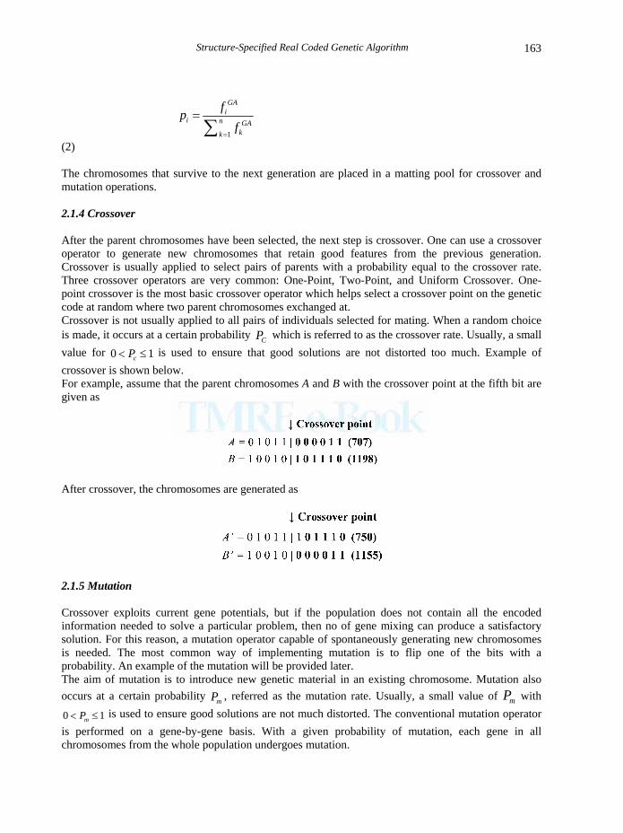
(2) The chromosomes that survive to the next generation are placed in a matting pool for crossover and mutation operations. 2.1.4 Crossover After the parent chromosomes have been selected, the next step is crossover. One can use a crossover operator to generate new chromosomes that retain good features from the previous generation. Crossover is usually applied to select pairs of parents with a probability equal to the crossover rate. Three crossover operators are very common: One-Point, Two-Point, and Uniform Crossover. One-point crossover is the most basic crossover operator which helps select a crossover point on the genetic code at random where two parent chromosomes exchanged at. Crossover is not usually applied to all pairs of individuals selected for mating. When a random choice is made, it occurs at a certain probability CP which is referred to as the crossover rate. Usually, a small value for 0 1cP< ≤ is used to ensure that good solutions are not distorted too much. Example of crossover is shown below. For example, assume that the parent chromosomes A and B with the crossover point at the fifth bit are given as

After crossover, the chromosomes are generated as

2.1.5 Mutation Crossover exploits current gene potentials, but if the population does not contain all the encoded information needed to solve a particular problem, then no of gene mixing can produce a satisfactory solution. For this reason, a mutation operator capable of spontaneously generating new chromosomes is needed. The most common way of implementing mutation is to flip one of the bits with a probability. An example of the mutation will be provided later. The aim of mutation is to introduce new genetic material in an existing chromosome. Mutation also occurs at a certain probability mP , referred as the mutation rate. Usually, a small value of mP with

0 1mP< ≤ is used to ensure good solutions are not much distorted. The conventional mutation operator is performed on a gene-by-gene basis. With a given probability of mutation, each gene in all chromosomes from the whole population undergoes mutation.


164

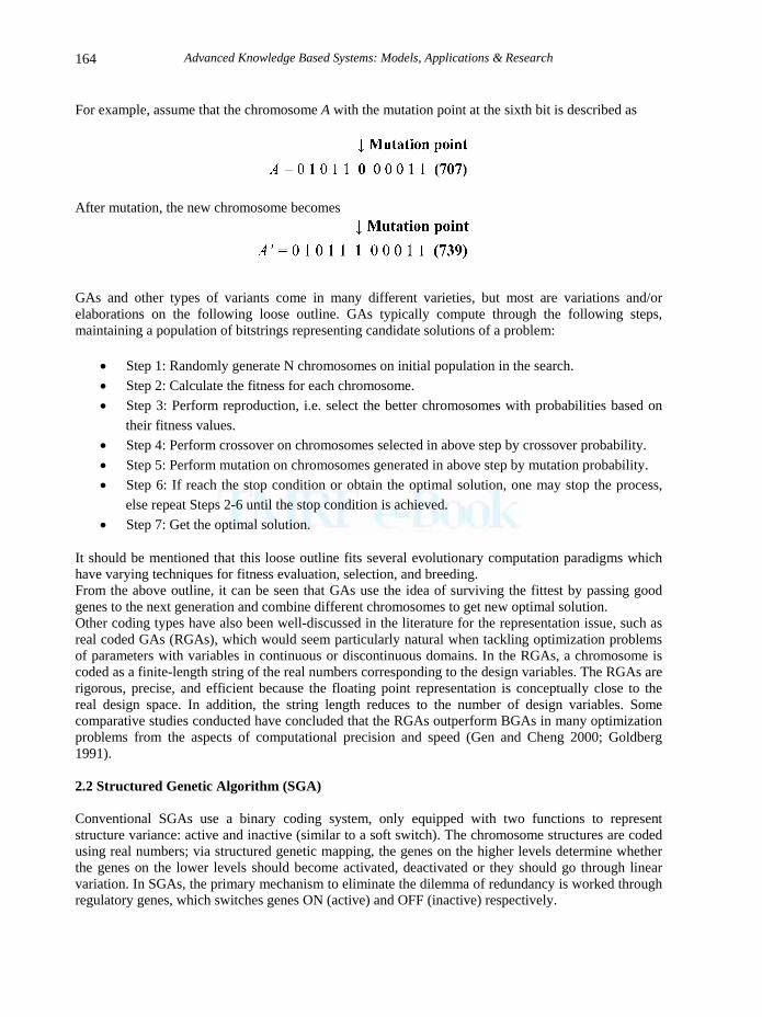
For example, assume that the chromosome A with the mutation point at the sixth bit is described as

After mutation, the new chromosome becomes

GAs and other types of variants come in many different varieties, but most are variations and/or elaborations on the following loose outline. GAs typically compute through the following steps, maintaining a population of bitstrings representing candidate solutions of a problem:

• Step 1: Randomly generate N chromosomes on initial population in the search. • Step 2: Calculate the fitness for each chromosome. • Step 3: Perform reproduction, i.e. select the better chromosomes with probabilities based on

their fitness values. • Step 4: Perform crossover on chromosomes selected in above step by crossover probability. • Step 5: Perform mutation on chromosomes generated in above step by mutation probability. • Step 6: If reach the stop condition or obtain the optimal solution, one may stop the process,

else repeat Steps 2-6 until the stop condition is achieved. • Step 7: Get the optimal solution.

It should be mentioned that this loose outline fits several evolutionary computation paradigms which have varying techniques for fitness evaluation, selection, and breeding. From the above outline, it can be seen that GAs use the idea of surviving the fittest by passing good genes to the next generation and combine different chromosomes to get new optimal solution. Other coding types have also been well-discussed in the literature for the representation issue, such as real coded GAs (RGAs), which would seem particularly natural when tackling optimization problems of parameters with variables in continuous or discontinuous domains. In the RGAs, a chromosome is coded as a finite-length string of the real numbers corresponding to the design variables. The RGAs are rigorous, precise, and efficient because the floating point representation is conceptually close to the real design space. In addition, the string length reduces to the number of design variables. Some comparative studies conducted have concluded that the RGAs outperform BGAs in many optimization problems from the aspects of computational precision and speed (Gen and Cheng 2000; Goldberg 1991). 2.2 Structured Genetic Algorithm (SGA) Conventional SGAs use a binary coding system, only equipped with two functions to represent structure variance: active and inactive (similar to a soft switch). The chromosome structures are coded using real numbers; via structured genetic mapping, the genes on the higher levels determine whether the genes on the lower levels should become activated, deactivated or they should go through linear variation. In SGAs, the primary mechanism to eliminate the dilemma of redundancy is worked through regulatory genes, which switches genes ON (active) and OFF (inactive) respectively.


165

The central feature of the SGA is its use of redundancy and hierarchy in its genotype. In the structured genetic model, the genomes are embodied in the chromosome and are represented as sets of binary strings. The model also adopts conventional genetic operators and the survival of the fittest criterion to evolve increasingly fit offspring. However, it differs considerably from the simple GAs while encoding information in the chromosome. The fundamental differences are as follows:

• The SGA interprets chromosomes as hierarchical genomic structures. The two-level structured genomes are illustrated as in Figure 1.

• Genes at any level can either be active or inactive. • “High level” genes activate or deactivate sets of lower level genes.

3a2a

21a 22a 23a 31a 32a 33a

1a

11a 12a 13a

1a 2a 3a 11a 12a 13a 21a 22a 23a 31a 32a 33a

Figure 1. A two-level structure of SGA (Dasgupta and Mcgregor 1992) Thus, a single change at higher level represents multiple changes at lower levels in terms of genes which are active; it produces an effect on the phenotype that could only be achieved in simple GAs by a sequence of many random changes. Genetic operations altering high-level genes result in changes in the active elements of the genomic structure and hence control the development of the fitness of the phenotype. Basically, SGA woks as a form of long term distributed memory that stores information, particularly genes once highly selected for fitness. The major advantage of using real-valued coding over binary coding is its high precision in computation. Moreover, the real-valued coding chromosome string is much shorter in the string length. 3. REAL CODED STRUCTURED GENETIC ALGORITHM (RSGA) To increase computation effectiveness, the RSGA combines the advantages of RGA with SGA. Its chromosome structure is coded using real numbers; via structured genetic mapping, the genes on the higher levels, named control genes, determine whether the genes on the lower levels, named parameter genes, should become activated, deactivated or should the genes go through linear ratio variation between the activated and deactivated statuses. RSGAs are equipped with three operations: activate, deactivate, and linear ratio variation. The genetic algorithm used in this section is real coded. The real number encoding has been to confirmed to have better performance than binary encoding for constrained optimization. Because of the conventional


166

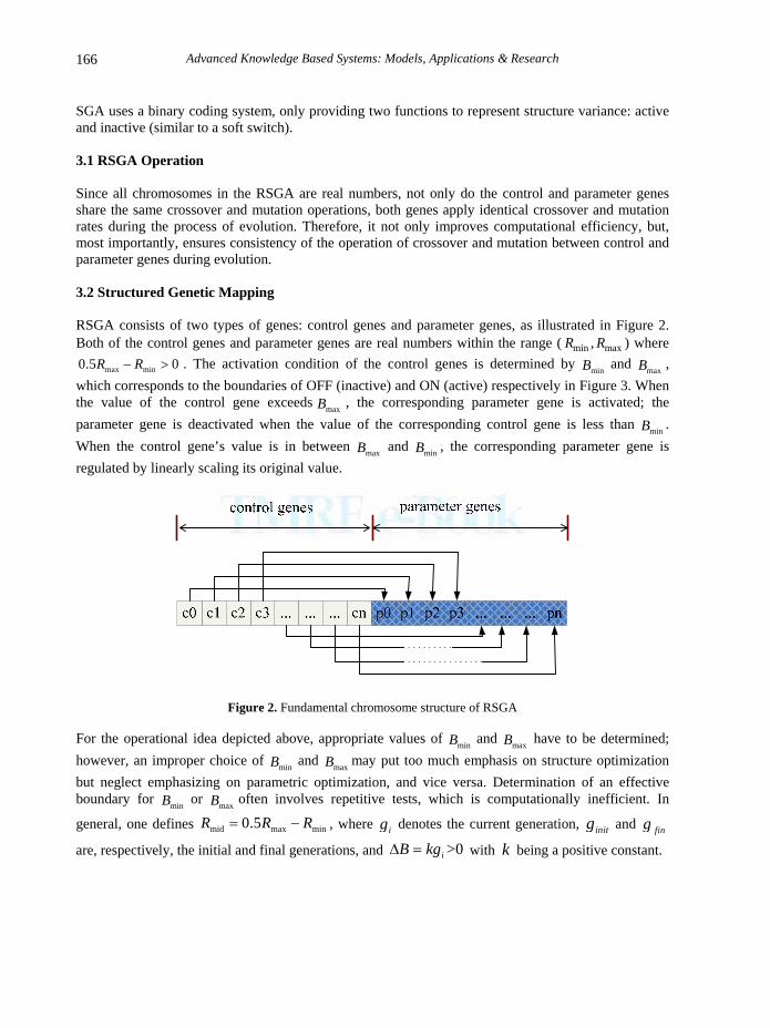
SGA uses a binary coding system, only providing two functions to represent structure variance: active and inactive (similar to a soft switch). 3.1 RSGA Operation Since all chromosomes in the RSGA are real numbers, not only do the control and parameter genes share the same crossover and mutation operations, both genes apply identical crossover and mutation rates during the process of evolution. Therefore, it not only improves computational efficiency, but, most importantly, ensures consistency of the operation of crossover and mutation between control and parameter genes during evolution. 3.2 Structured Genetic Mapping RSGA consists of two types of genes: control genes and parameter genes, as illustrated in Figure 2. Both of the control genes and parameter genes are real numbers within the range ( min max,R R ) where

max min0.5 0R R− > . The activation condition of the control genes is determined by minB and maxB , which corresponds to the boundaries of OFF (inactive) and ON (active) respectively in Figure 3. When the value of the control gene exceeds maxB , the corresponding parameter gene is activated; the parameter gene is deactivated when the value of the corresponding control gene is less than minB . When the control gene’s value is in between maxB and minB , the corresponding parameter gene is regulated by linearly scaling its original value.

Figure 2. Fundamental chromosome structure of RSGA For the operational idea depicted above, appropriate values of minB and maxB have to be determined; however, an improper choice of minB and maxB may put too much emphasis on structure optimization but neglect emphasizing on parametric optimization, and vice versa. Determination of an effective boundary for minB or maxB often involves repetitive tests, which is computationally inefficient. In

general, one defines mid max min0.5R R R= − , where ig denotes the current generation, initg and fing

are, respectively, the initial and final generations, and >0iB kgΔ = with k being a positive constant.


167

Figure 3. Activation functions of the control genes The boundary sizing technique can resolve the problem depicted above. The RSGA first acts like a soft switch during the early stage of evolution, provides only ON or OFF functions, emphasizing structural optimization. As the evolution proceeds, the boundary increases progressively with generation number such that linear scaling is put into effect to promote additional emphasis on the parameter optimization. At the end of the generation, the boundaries of minB and maxB will replace the entire range, focusing only on parameter optimization. This ensures that this structure is optimized before shifting the focus into the optimization of parameters. To explain, the mathematical model of the fundamental chromosome structure is defined as follows

1, ([ ], [ ]), , , 1, ,pini i i iX C P c p c p i n×=< > = ∈ ∈ = K (3)

where

1

1[ ] n

pii

in n

X x=

⎛ ⎞⎜ ⎟× +⎜ ⎟⎝ ⎠

=∑

represents an ordered set consisting of the control genes’ strings 1[ ]i nC c ×=

and the parameter genes’ string 1

1[ ] n

pii

in

P p=

⎛ ⎞⎜ ⎟×⎜ ⎟⎝ ⎠

=∑

. The structured genetic mapping from C to P is

defined as

, ,X C P C C P=< >=< ⊗ >% % (4) where [ ] [ ]i iP c p= ⊗% with

max

min max

min

ififif

i i

i i i

i

p , B cp p t , B <c B

, c Bφ

≤⎧⎪ <⎨⎪ ≤⎩

% (5)

⊗ is called the soft genetic switch which determines the status of each element in the parameter gene string (determined by (5)), φ is the bit denoting the corresponding parameter gene to be ignored in the

later evolution process, min

max min

ic BtB B

−=

− denotes the effective gain for ic within the boundary of minB

and maxB .


168

Example:

A randomly generated chromosome is given in the follows where max 5B = and min 5B = − . ,X C P=< >

[ 6 -5 -2 3 9 -6, -3 7 5 -1 2 -3

C P644444474444448

]

644444474444448

[-6 5 2 -3 -9 6, 3 -7 -5 1 -2 3]

[ 6 -5 -2 3 9 -6, -3 7 5 -1 2 -3

C P644444474444448

]

644444474444448

[-6 5 2 -3 -9 6, 3 -7 -5 1 -2 3]

Since

1 min 1

2 max 2 2

3 min max 3 3 3 3

4 min max 4 4 4 4

5 min

6 5 OFF 5 5 ON 7 2, 2 3.5, where 0.7 3, 3 0.2, where 0.2 9 5 OFF

c B pc B p pc B B p p t tc B B p p t tc B p

φ=− < =− ⇒ → == ≥ = ⇒ → = =−= < < → = =− ==− <− < → = = ==− < =− ⇒ →

%

%

%

%

%5

6 max 6 6 6 5 ON 3c B p pφ=

= > = ⇒ → = =%

,X C P=< > X% :

[6 -5 -2 3 9 -6, -3 1.5 -0.8 2

C P

φ φ

%

644444474444448

]

64444444744444448

[-6 5 2 -3 -9 6, -7 -3.5 0.2 3 ]φ φ

P%

[6 -5 -2 3 9 -6, -3 1.5 -0.8 2

C P

φ φ

%

644444474444448

]

64444444744444448

[-6 5 2 -3 -9 6, -7 -3.5 0.2 3 ]φ φ

P%

3.3 Genetic Mathematical Operations Similar to standard GAs, the RSGA involves three major genetic operations: selection, crossover, and mutation. Since both control genes and parameter genes are real numbers, unlike the conventional SGAs (Tang, Man and Gu 1996), the RSGA utilizes the same mathematical operations to conduct crossover and mutation, which is less time consuming and requires less computational burden. In conventional SGAs, the control and parameter genes were coded as binary and real numbers, respectively; therefore, the crossover and mutation for the two parts require different mathematical mechanism which may result in uneven evolution. 3.3.1 Initial Population As for RGSs, the initial population consisting a certain amount of randomly generated individuals (in the form of (3)), each represented by a real numbered string, is created. Each of these strings (or chromosomes) represents a possible solution to the search problem.


169

3.3.2 Fitness The algorithm works toward optimizing the objective function, which consists of two parts corresponding, respectively, to structure and parameters as follows:

( ) ( ) (1 ) ( )tot s pJ X J X J Xρ ρ= + − (6) with sJ being the normalized index of structure complexity; pJ , the normalized performance index;

[0, 1]ρ ∈ being the weighting factor representing the desired emphasis on structure complexity. To employ the searching algorithms, the targeted solutions are commonly related to the fitness function ( )f ⋅ . A linear equation can be introduced to relate the total cost index ( )totJ ⋅ to ( )f ⋅ . The linear mapping between ( )totJ ⋅ and ( )f ⋅ , called as the “windowing” technique, is given as

[ ]( ) ( )tot l uf J J fμ⋅ = ⋅ − + (7)

which u l

l u

f fJ J

μ −=

−, with uJ and lJ denoting the largest and smallest values of ( )totJ ⋅ within all

individuals evaluated in the current generation, and lf and uf being the constant minimum and maximum fitness values assigned, respectively, to the worst and best chromosomes. 3.3.3 Selection In this phase, a new population is created from the current generation. The selection operation determines which parent participates in the production of offsprings for the next generation, analogous to the survival of the fittest in the process of natural selection. Usually, members selected for mating depends on their individual fitness values. A common way to implement selection is to set the selection probability equal to

1

mi jj

f f=∑ , where if is the fitness value of the i-th member, and m is

the population size. A higher probability tends to be assigned to chromosomes associated with higher fitness value among the population. 3.3.4 Crossover Crossover plays the role of mixing two chosen chromosomes as in RGAs. As in the usual GAs, the number of individuals joining the operation is determined by the crossover probability cp , usually

0.5 0.9cp≤ ≤ . The crossover of the randomly selected pairs of individuals is a combination of an extrapolation/interpolation method with a crossover process. It starts from extrapolation and shifts to interpolation if the parameters of the offspring exceed the permissible range. Interpolation avoids parameters from going over the admissible range during the boundary value search. The operation is determined by

( )( )

,,

di di di mi

mi mi di mi

x x x xx x x x

λλ

= − −⎧⎨ = + −⎩

%

% max minif > or <di mix R x R , (8)


170

( )( )

,,

di di di mi

mi mi di mi

x x x xx x x x

λλ

= + −⎧⎨ = − −⎩

%

% min maxif mi diR x x R≤ ≤ ≤ , (9)

, { }di mix x φ∉ , 2j i n≤ ≤ , 1 2j n< < (10)

0 1 i

fin

gg

λ λ⎛ ⎞

= −⎜ ⎟⎜ ⎟⎝ ⎠

, di mix x≥ (11)

where the subscripts m and d are used to discriminate the parents: mom and dad, i denotes the i-th elements in the parent chromosomes, ( , d mx x% % ) are offsprings of ( , d mx x ), 0 [0,1]λ ∈ is a uniform random number, the parameter j is a random number in the pair of parents to designate the crossover point:

0ceil(2 )j n λ= × (12)

Note that both control and parameter genes apply the same crossover operation to generate new individuals. This unified mechanism avoids the need to utilize two types of crossover operators with different attributes as required in traditional SGAs. The unified mechanism results in better computation efficiency and consistency of chromosome crossover. 3.3.5 Mutation

The mutation operator applies individually for the randomly chosen individuals. The number of individuals to be varied is determined by the mutation probability mp , 0 1mp< . The operator adopts the technique of non-uniform mutation which changes the gene in a chromosome with each generation via

max

min

( , ), if 0( , ), if 1

ij ij ijij

ij ij ij

x g x x hx

x g x x h+ Δ − =⎧⎪= ⎨ −Δ − =⎪⎩

% (13)

0( , ) 1 ii

fin

gg yg

βλ⎛ ⎞

Δ = −⎜ ⎟⎜ ⎟⎝ ⎠

(14)

where { }ijx φ∉ , the random integer number {0,1}h∈ , maxijx ( minijx ) is the maximal (minimal) j-th element of the i-th individual in the current generation, and β is a scaling factor. The above mechanism is employed so that the control genes affect the parameter genes during the early stage of evolution and optimize the structure. As the process of evolution progresses, the control genes loose their effect; the algorithm gradually tends to optimize the parameter genes. The structured genetic mapping for all individuals, from the control genes to parameter genes, defined by (4) is performed after mutation. A new generation with m offsprings is bred. The process repeats until the fittest individual is generated.


171

3.3.6 Termination Criterion The algorithm produces new generations until the terminal condition is reached. The algorithm terminates when the generation number reaches a specific number or the fitness value of the best fitted individual converge to an acceptable level. And then the individual with maximum fitness function is chosen to be the solution. 4. FILTER DESIGN USING RSGA

This section demonstrates a useful application of RSGAs in filter designs, in which the objective is incorporated to the algorithm to tackle the digital IIR filter design.

In signal processing, the function of a filter is to remove unwanted parts of the signal, such as random noise, or extract useful parts of the signal, such as the components lying within a certain frequency range. A typical digital filter design problem involves determination of a set of filter coefficients to meet certain specifications such as the width of the passband ( pω ) and the corresponding gain, the

width of the stopband ( sω ) and the attenuation therein, the band edge frequencies and the peak ripple tolerable magnitudes (

pδ ,sδ ) in the passband and stopband. Figure 4 shows related filtering

specifications for the low pass filter (LPF), high pass filter (HPF), band pass filter (BPF), and band stop filter (BSP).

π

π

π

π

pδ

sδ ω

ω

ω

ω

pδ

sδ

pδ

sδ

pδ

sδ

sωpω

sω pω

1sω 1pω 2pω 2sω

1sω1pω 2pω2sω

Figure 4. Specifications of LP, HP, BP, and BS filters Two types of digital filters are commonly encountered, i.e. infinite impulse response (IIR) and finite impulse response (FIR) filters. An IIR filter has an impulse response function that is non-zero over an infinite length of time. This is in contrast to the FIR filter, which possesses fixed-duration impulse responses. An IIR filter may continue to respond indefinitely, whereas the impulse response of an Nth-order FIR filter only lasts for N+1 sampling periods.


172

4.1 IIR Filtering Model (Shynk 1989) In the time domain, the generic N th-order difference equation defines how the output signal is related to the input signal that represents an IIR filter described by

1 0

[ ] [ ] [ ]N M

i ii i

y n a y n i b x n i= =

− − = −∑ ∑

(15)

where M is the feedforward filter order, N is the feedback filter order, ib are the feedforward filter

coefficients, ia are the feedback filter coefficients. This equation shows how to compute the next

output sample [ ]y n , in terms of the past outputs [ ]y n i− , the present input [ ]x n , and the past inputs

[ ]x n i− . Applying the filter to an input in realization form is depending on the exact order of

evaluation.

The transfer function (TF) ( )H z of the IIR filter possesses the following form:

1 20 1 2

1 21 2

( )( )( ) 1

MM

NN

b b z b z b zB zH zA z a z a z a z

− − −

− − −

+ + + += =

+ + + +L

L, M N≤

(16)

or

1 2

1 2

21 2

1 1

21 2

1 1

( ) ( )( )

( ) ( )

M M

j l li iN N

i k ki i

z b z b z bH z K

z a z a z a

= =

= =

+ + +=

+ + +

∏ ∏

∏ ∏, M N≤

(17)

where the orders of the numerator and denominator polynomials in (17), according to the degree of z , are, respectively, 1 22M M M= + and 1 22 ,N N N= + K is a constant, and ia , ib , 1ia , 2ia , 1ib , 2ib are coefficients of the corresponding terms. 4.2 Constraints on IIR Digital Filter

• The order of the denominator polynomial is larger than or equal to that of the numerator polynomial:

deg( ( )) deg( ( ))A z B z≥ (18)


173

where deg( ( ))p z denotes the degree of the polynomial ( )p z .

• To ensure stability, the roots of the denominator polynomial (i.e. poles of ( )H z ) must lies

inside the unit circle:

[ ]mag poles( ( )) 1H z ≤ (19)

where poles( ( ))H z denotes the poles of ( )H z . 4.3 Digital IIR Filter Design A typical digital filter design problem involves the determination of a set of filter coefficients which meet performance specifications, such as passband width and corresponding gain, widths of the stopband and attenuation, band edge frequencies, and tolerable peak ripple in the passband and stopband. The RSGA is capable of coding the system parameters into a hierarchical structure. A complete gene string representing ( )H z consists of 1 1 2 2 1M N M N+ + + + control genes and

1 1 2 22( ) 1M N M N+ + + + parameter genes. The coefficients of the first- and second-order models are controlled by control genes, which determine the corresponding coefficients whether to turn ON or OFF or should they go through linear scaling.

The performance index totJ in (6) for an optimal digital IIR filter design is defined as

( ) ( ) (1 ) ( ) ( )tot s pp psJ J J Jρ ρ ⎡ ⎤⋅ = ⋅ + − ⋅ + ⋅⎣ ⎦ (20) where

max1 Log( 1)sJ N Nδ

= − +

(21) with { }max ,sgn( )N Mδ ε= − , ε , a small positive constant, maxdN , the assigned maximum order of the denominator polynomial; ppJ and psJ ensure that the frequency responses are confined within the prescribed frequencies listed in Table 1; for each filter specification, the tolerable error of passband and stopband are defined as

1

1

( ) 1, if ( ) 1

1 ( ) , if ( ) 1

ppb pb

ppb pb

rj j

pbpp r

j jp p

pb

H e H eJ

H e H e

ω ω

ω ωδ δ

=

=

⎧− >⎪

⎪= ⎨⎪ − − < −⎪⎩

∑

∑, pbω∀ ∈passband (22)

and

1

( ) , if ( )s

sb sb

rj j

ps s ssb

J H e H eω ωδ δ=

= − >∑ , sbω∀ ∈ stopband (23)


174

with pδ and sδ representing the ranges of the tolerable error for bandpass and bandstop, respectively;

pr and sr are the numbers of equally spaced grid points for bandpass and bandstop, respectively. The magnitude response is represented by discrete frequency points in the passband and stopband. 4.4 Simulation Study The first experiment is to design digital filters that maximize the fitness function within certain frequency bands as listed in Table 1.

The IIR filter models originally obtained are as follows (Tang, Man, Kwong and Liu 1982)

2

2

( 0.6884)( 0.0380 0.8732)( ) 0.0386( 0.6580)( 1.3628 0.7122)LPz z zH zz z z+ − +

=− − +

2

2

( 0.4767)( 0.9036 0.9136)( ) 0.1807( 0.3963)( 1.1948 0.6411)HPz z zH zz z z− + +

=+ + +

2 2

2 2

( 0.8846)( 0.9033)( 0.0498 0.8964)( 0.031 0.9788)( ) 0.077( 0.0497)( 0.0592)( 0.5505 0.5371)( 0.5551 0.5399)BP

z z z z z zH zz z z z z z− + − − + −

=+ − − + + +

2 2

2 2

( 0.4230 0.9915)( 0.4412 0.9953)( ) 0.4919( 0.5771 0.4872)( 0.5897 0.4838)BSz z z zH zz z z z+ + − +

=+ + − +

For comparison, the RSGA was applied to deal with the same filter design problem. The fitness function defined in (20) was adopted to determine the lowest ordered filter with the least tolerable error. The weighting factor ρ was set to 0.5 for both LPF and HPF, and 0.7 for BPF and BSF. M and N were set to be 5. The genetic operational parameters adopted the same settings as those of the HGA proposed by Tang et al. (1982). The population size was 30, the crossover and mutation probabilities were 0.8 and 0.1, respectively, and the maximum iteration were 3000, 3000, 8000, and 8000 for LPF, HPF, BPF and BSF, respectively. By running the design process 20 times, the best results using the RSGA approach were

2

2

( 0.2562)( 0.448 1.041)( ) 0.054399( -0.685)( 1.403 0.7523)LPz z zH zz z z+ − +

=− +

2

2

( 1.341)( 0.8952 0.9913)( ) 0.063462( 0.5766)( 1.332 0.7277)HP

z z zH zz z z− + +

=+ + +

2 2

( 1.362)( 1.048)( 1.132)( 0.6244)( ) 0.071458( 0.4969 0.6853)( 0.4894 0.6929)BP

z z z zH zz z z z

+ + − −=

− + + +


175

2 2

2 2

( 0.3241 0.8278)( 0.3092 0.8506)( ) 0.44428( 0.8647 0.5233)( 0.8795 0.5501)BSz z z zH zz z z z+ + − +

=− + + +

For further comparison, define pε and sε as the maximal ripple magnitudes of passband and stopband:

{ }1 min ( )pbjp H e ωε = − , pbω∀ ∈passband (24)

{ }max ( )sbjs H e ωε = , sbω∀ ∈ stopband (25)

Table 1. Prescribed frequency bands

Filter Type Bandpass Bandpstop

LP 0 0.2pbω π≤ ≤ 0.3 sbπ ω π≤ ≤

HP 0.8 pbπ ω π≤ ≤ 0 0.7sbω π≤ ≤

BP 0.4 0.6pbπ ω π≤ ≤ 0 0.250.75

sb

sb

ω ππ ω π

≤ ≤≤ ≤

BS 0 0.25

0.75pb

pb

ω π

π ω π

≤ ≤

≤ ≤ 0.4 0.6sbπ ω π≤ ≤

The filtering performances within the tolerable passband and stopband are summarized in Table 2. The ranges of the tolerable error for bandpass pδ and bandstop sδ in the RSGA approach are less than the

HGA. Figure 5 shows the frequency responses of LPF, HPF, BPF and BSF with two approaches. The

RSGA yielded filters with lower passband pε and stopband sε ripple magnitudes, see Table 3.

Table 2. Comparison of filtering performance

RSGA Approach

Passband Tolerance Stopband Tolerance

0.9 ( ) 1pbjH e ω≤ ≤

( 0.1)pδ =

( ) 0.15sbjH e ω ≤

( 0.15)sδ =


176

HGA Approach

Passband Tolerance Stopband Tolerance

0.89125 ( ) 1pbjH e ω≤ ≤

( 0.10875)pδ =

( ) 0.17783sbjH e ω ≤

( 0.17783)sδ =

(1a) (1b)

(2a) (2b)

(3a) (3b)


177

(4a) (4b)

Figure 5. Frequency responses of LPF (1a, 1b), HPF (2a, 2b), BPF (3a, 3b), BSF (4a, 4b) by using the RSGA and

HGA approaches

Table 3. Results for LPF, HPF, BPF, BSF

RSGA Approach

Filter Type Passband Ripple Magnitude pε Stopband Ripple Magnitude sε

LP 0.0960 0.1387

HP 0.0736 0.1228

BP 0.0990 0.1337

BS 0.0989 0.1402

HGA Approach

Filter Type Passband Ripple Magnitude pε Stopband Ripple Magnitude sε

LP 0.1139 0.1802

HP 0.0779 0.1819

BP 0.1044 0.1772

BS 0.1080 0.1726

Table 4 shows that the RSGA approach requires less generation to achieve the desired design specifications under the same design requirements. Table 5 shows that the resulting BP filter is structurally simpler.

Table 4. Required generation number for convergence

Generation Filter Type

RSGA Approach HGA Approach

LP 1242 1649

HP 879 1105

BP 3042 3698

BS 4194 7087


178

Table 5. Lowest Filter Order

Filter order

Filter Type RSGA Approach HGA Approach

LP 3 3

HP 3 3

BP 4 6

BS 4 4

5. CONTROL DESIGN USING RSGA This section presents one of the major applications of RSGAs in control design. 5.1 Control Design Description Consider the closed-loop control system as shown in Figure 6, where ( )nP s is the nominal plant model; ( )P sΔ , the multiplicative unmodeled dynamics; ( )C s , the controller; ( )H s , the sensor model;

( )d t , the reference input; ( )u t , the control command; ( )y t , the plant output; ( )e t , the tracking error. Modeling inaccuracy is considered due to uncertain effects or modeling errors.

Let the uncertain plant model ( )P s be described by

( ) [ ]( ) 1 ( )nP s P s P s= +Δ (26) where ( )P sΔ satisfies

( ) ( )tP j W jω ωΔ ≤ , ω∀ (27) In which is a stable rational function used to envelop all possible unmodeled uncertainties.

( ) ( )1nP s P s+ Δ⎡ ⎤⎣ ⎦cue

+−

d y

( )H s

( )C s

Figure 6. Typical uncertain closed-loop feedback control scheme

The chromosome structure of RSGA representation in Figure 2 is applied to deal with the robust control design problem where the generalized TF of a robust controller is given by


179

1 2

1 2

21 2

1 1

21 2

1 1

( ) ( )( )

( ) ( )

M M

j l lj lN N

i k ki K

s b s b s bC s K

s a s a s a

= =

= =

+ + +=

+ + +

∏ ∏

∏ ∏

% %

% % (28)

where K is a constant, ia , jb , 1ka , 2ka , 1lb , 2lb are the coefficients of the corresponding polynomials. 5.1.1 Frequency Domain Specifications H∞ control theory is a loop shaping method of the closed-loop system that -normH∞ is minimized under unknown disturbances and plant uncertainties (Green and Limebeer 1995). The principal criterion of the problem is to simultaneously consider robust stability, disturbance rejection as well as control consumption. 5.1.1.1 Sensitivity Constraint The problem can be defined as

( )1 1sG W S jω∞< (29)

where ( ) sup ( )A j A j

ωω ω

∞= with ( )A s being a stable rational function; ( ) 1

1 ( ) ( ) ( )nS s P s C s H s= +

, the

sensitivity function; ( )sW s , the weighting function that possesses a sufficiently high gain in low frequency to achieve disturbance suppression and eliminate the steady-state error. 5.1.1.2 Control Constraint To fulfill the requirement of minimizing control commands at higher frequency, an appropriate weighting function ( )rW s should be introduced. To fulfill the constraint, the following criterion is considered:

( )2 1rG W R jω∞< (30)

where ( )( ) 1 ( ) ( ) ( )n

C sR s P s C s H s= + is the control TF for the nominal closed-loop system. The inequality

guarantees internal stability if there is no right-half plane pole/zero cancellation in the controller and plant. 5.1.1.3 Robust Stability Constraint The controller ( )sC is required to maintain closed-loop stability when encountering uncertainty

( )P sΔ ; the requirement can be assured when the following inequality is satisfied:


180

( )( )1 , P j

T jω ω

ωΔ < ∀ (31)

where ( ) 1 ( )T s S s= − is the complementary sensitivity function.

Under the assumption (31), the robust stability constraint can be expressed as

( )3 1tG W T jω∞< (32)

From the viewpoint of the weighting function, ( )tW s defined in (27) works such that the resulting controller does not stimulate higher resonant frequency of the plant ( )P s . 5.1.2 Weighting Functions In a nominal closed-loop system, if the bandwidth is required to be at cω then the requirement can be assured by introducing an appropriate weighting function ( )tW s with high gain at higher frequencies and the corner frequency close to cω . In addition to consider disturbance rejection, ( )sW s is designed to eliminate the steady-state error. To make the steady-state error equal to zero with respect to the step input ( )d t , one must have

( )0 0S = , i.e. the weight should approach infinity when ω approaches zero. Under the invariant

relationship ( ) ( ) 1S j T jω ω+ = , ω∀ , the corner frequency cω can be approximately chosen to complement the asymptotic frequency property of ( )tW s . The design of the weighting function ( )rW s is similar to that of ( )tW s , where the objective is to avoid excessive control commands at higher frequencies. 5.1.3 Time Domain Specifications Evaluation of the transient response can be performed via an effective method by relating directly to the tracking performance, opposed to the conventional method of examining frequency domain specifications indirectly. The objective function can be chosen to reflect the overall performance

1 2 3 ,p OJ M Tr Essα α α= + +% 3

11i

iα

=

=∑ (33)

where 0iα ≥ are the scalars included to weigh the relative importance of three transient response indices; OM is the normalized maximum overshoot, Tr is the normalized rise time, and Ess is the normalized steady-state error. 5.1.4 Multiple-Objective Optimization Multiple-objective optimization problems are usually quite different from the single-objective ones. One attempts to obtain the best solution which is absolutely superior to all other alternatives. This section considers a performance index to reflect the control requirement and overall system


181

performance, i.e. sensitivity suppression, control consumption, good transient response, and simpler controller’s structure. The objective is to search for an appropriate controller that makes each objective function achieve the best compromise. Although a complicated H∞ controller usually possesses superior performance, a simpler structure with acceptable performance is more practical. Therefore, the objective functions considered should contain not only performance but also structural information of the controller. For the current problem, define a generalized constrained multiobjective model as follows

( )min OF ⋅%

(34)

( )s.t. 1 , 1, 2, 3iG i⋅ ≤ =

(35)

and the multiobjective function are defined as follows

( 1 )O s pF J Jβ β= + −% % % (36) where

,ds

m

nJN

=%%%

max0

gqgeβ β σ

−⎛ ⎞= +⎜ ⎟⎜ ⎟

⎝ ⎠%

pJ% is time domain response measure, sJ% is the normalized controller order, dn% is the order of the denominator polynomial,

0 [0,1]β ∈ is a weighting factor that represents the desired emphasis on structure complexity, g is the current generation, maxg is the maximum number of generations, q is a shaping factor, and σ% is a small positive constant which avoids the weight of sJ% from zero. The minimization formulation can be transformed into a fitness evaluation ( )f ⋅% which is a measure evaluating suitability of a candidate and is to be used in the solution searching process. The fitness value determines the probability that a candidate solution is selected to produce possible solutions in the next generation. To apply the RSGA, a linear equation is introduced to connect ( )OF ⋅% and ( )f ⋅% as follows

( ) ( )Of Fμ ζ⋅ = ⋅ +% % (37)

where u l

Ol Ou

f fF F

μ −=

−

% %

% % and ufζ μ= −% with OuF% and OlF% being the largest and smallest values evaluated

in the current generation, and uf% and lf% being the corresponding fitness values, respectively.


182

Then, applying the penalty function makes infeasible solutions have less fitness than the feasible ones. To achieve this aim, a constrained multi-objective fitness function can be applied:

( ) ( ) ( )F f p⋅ = ⋅ ⋅%% (38) where the penalty function ( )p ⋅ is applied for adjusting the value of penalty in the constrained

multiple-objective function at each generation and to differentiate feasible and infeasible candidates:

3

max1

( )1( ) 13 ( )

i

i i

CpC=

⎛ ⎞Δ ⋅⋅ = − ⎜ ⎟Δ ⋅⎝ ⎠

∑

(39) and

{ }( ) max 0, ( ) 1i iC GΔ ⋅ = ⋅ − , { }max ( ) max , ( )i p iC CηΔ ⋅ = Δ ⋅

in which ( )iCΔ ⋅

is the value of violation for i-th constraint, maxiCΔ is the maximum violation for i-th

constraint in the current population, and pη is a small positive number. One applies the penalty function to adjust the values of penalties in the constrained multi-objective fitness function at each generation to differentiate between feasible and infeasible parameters. The method raises efficiency in the searching for optimal solution. 5.2 Simulation Study 5.2.1 Robust Control for Non-Minimum Phase Plant Consider a typical H∞ control design problem with control constraints. The non-minimum phase plant with a right-half plane zero is given by

2( )( 0.01)( 3)

sP ss s

−=

+ −

and the weighting function corresponding to the control constraint is

0.01 0.1( )100r

sW ss

+=

+

Synthesis of the H∞ control problem subject to the constraint (30) was solved by applying Matlab-Robust Control Toolbox (Balas, Chiang, Packard and Safonov 1995) and the RSGA. The former yielded an optimal H∞ controller given as

4 2 6

3 2 5 6

2.486 10 2.486 10 2488( )1.094 1.5 10 1.659 10Matlab

s sC ss s s

⋅ + ⋅ −=

+ + ⋅ − ⋅


183

For the RSGA approach, the population size was chosen to be 30; crossover rate, 0.8CP = ; mutation rate, 0.2mP = ; the maximum number of generations, 100; 0 0.5ρ = . The resulting controller was obtained as

2

230.2555( 0.006682)( )12.057 159.139RSGA

sC ss s

−=

+ −

This gives 2G in (30) as 0.0348 . The results of transient responses displayed in Figure 7 show better performance of the RSGA approach than that obtained by Matlab-Robust Control Toolbox. Figure 7(1) shows faster response, Figure 7(2) show smaller control commands, and Figure 7(3) shows less tracking errors of the RSGA design.

(1a) (1b)

(2a) (2b)


184

(3a) (3b) Figure 7. Step response (1a, 1b), control command (2a, 2b) and tracking error (3a, 3b) for the unstable plant with

a non-minimum phase zero by using the RSGA approach and MATLAB-Robust Control Toolbox 5.2.2 Control Design for MBDCM The TF of a micro brushless DC motor (MBDCM) Pittman Express 3442S004-R3 for precision positioning, while no load, is given by

8 3 2

0.0486( )7.47 10 0.0006 0.1097

P ss s s−=

× + +

The weighting functions of the sensitivity function and the control TFs were chosen, respectively, as follows

100( )500 1sW s

s=

+, 2

0.25( )10 100rW s

s s=

+ +

Figure 8 compares the structural variation between the RSGA and SGA during their evolution processes over generations. As it was displayed, the former exhibits more structural variations in the earlier generations but switched to optimizing the parameters later on. The conventional SGA also exhibits adequate structural variations; however, the structure converges slower than that of the RSGA. The controllers obtained by using the RSGA and SGA were given, respectively, as follows

( )31.8895 0.03835( )

0.03213RSGA

sC s

s+

=+

, ( )27.8991 0.04443

( )0.02823SGA

sC s

s+

=+

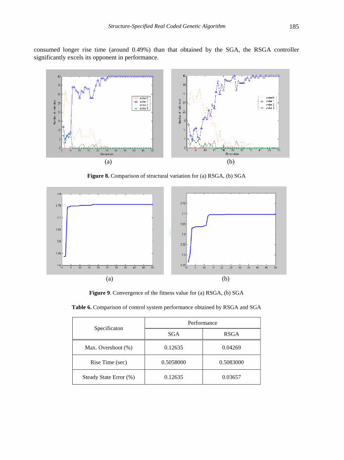
Comparison of convergence of the fitness values for both approaches is shown in Figure 9. It is seen that the RSGA converges at the generation 4 , whereas the SGA converges at the generation 14 . Also, the fitness value attained by the RSGA is 3.75 which is comparatively higher than 3.7 of the SGA. Table 6 summarizes performance of two designs. The RSGA controller yielded less overshoot and steady state error in transient responses than that of the SGA controller. Although the former system


185

consumed longer rise time (around 0.49%) than that obtained by the SGA, the RSGA controller significantly excels its opponent in performance.

(a) (b)

Figure 8. Comparison of structural variation for (a) RSGA, (b) SGA

(a) (b)

Figure 9. Convergence of the fitness value for (a) RSGA, (b) SGA

Table 6. Comparison of control system performance obtained by RSGA and SGA

Performance

Specificaton SGA RSGA

Max. Overshoot (%) 0.12635 0.04269

Rise Time (sec) 0.5058000 0.5083000

Steady State Error (%) 0.12635 0.03657


186

CONCLUSIONS This chapter introduces the mechanism of a class of GAs, giving special emphasis on the RSGA, a variant of GAs and SGAs. The RSGA is capable of simultaneously dealing with the structure and parameter optimization problems based on the real coded chromosome scheme. As it adopts the same crossover and mutation for genetic operations, it performs better in computational efficiency and results in even evolution of offsprings. Novelty of this genetic model also lies in redundant genetic material and an adaptive activation mechanism. For demonstration, the genetic search approach in the designs of digital filters and robust controllers are introduced. The results show that this GA model exhibits better performance in pursing solutions while compared with the existing GAs. References Ashlock, D. 2006. Evolutionary Computation for Modeling and Optimization. Springer. Balas, G. J., R. Chiang, A. Packard, and M. Safonov. 1995. Robust Control Toolbox. MathWorks,

Natick, MA. Bellas, F., J. A. Becerra, and R. J. Duro. 2009. Using promoters and functional introns in genetic

algorithms for neuroevolutionary learning in non-stationary problems. Neurocomputing Journal 72:2134-2145.

Chen, B. S., and Y. M. Cheng. 1998. A structure-specified H∞

optimal control design for practical applications: a genetic approach. IEEE Trans. Control System Technology 6:707-718.

Chen, J., E. Antipov, B. Lemieux, W. Cedeno, and D. H. Wood. 1999. DNA computing implementing

genetic algorithms, in Proc. DIMACS Workshop on Evolution as Computation, 39-51. Dasgupta, D., and D. R. Mcgregor. 1991. A structured genetic algorithm: the model and the first

results. Res. Rep. IKBS-2-91, Strathclyde University,U.K. Dasgupta, D., and D. R McGregor. 1992. Designing application-specific neural networks using the

structured genetic algorithm, in Proc. Int. Conf. Combinations of Genetic Algorithms and Neural Networks, 87-96.

Dasgupta, D., and D. R. McGregor. 1992. Nonstationary function optimization using the structured

genetic algorithm, in Proc. Int. Conf. Parallel Problem Solving from Nature, 145-154. Etter, D. M., M. J. Hicks, and K. H. Cho. 1982. Recursive adaptive filter design using an adaptive

genetic algorithm, in Proc. IEEE Int. Conf. ICASSP, 635-638. Gen, M., and R. Cheng, 2000. Genetic Algorithms and Engineering Optimization. New York: Wiley. Goldberg, D. E. 1991. Real-coded genetic algorithms, virtual alphabets and blocking. Complex

Systems 5:139-167. Green, M., and D. J. N. Limebeer. 1995. Linear Robust Control. NJ: Prentice-Hall, Englewood Cliffs. Hlavacek, M., R. Kalous, and F. Hakl. 2009. Neural network with cooperative switching units with

application to time series forecasting, in Proc. WRI World Congress on Computer Science and


187

Information Engineering, 676-682, Holland, J. H. 1975. Adaptation in Natural and Artificial Systems. Cambridge: MIT Press, MA. Jamshidi, M., R. A. Krohling, L. S. Coelho, and P. J. Fleming. 2002. Robust Control Systems with

Genetic Algorithms. CRC Press. Kaji, B., G. Chen, and H. Shibata. 2003. Design of reduced-order controller by using real-coded

genetic algorithm, in Proc. Southeastern Symposium System Theory, 48-52. Lai, C. C., and C. Y. Chang. 2004. A hierarchical genetic algorithm based approach for image

segmentation, in Proc. IEEE Int. Conf. on Networking, Sensing and Control, 1284-1288. Lin, C. L., and H. Y. Jan. 2005. Mixed/multiobjective PID control for a linear brushless DC motor: an

evolutionary approach. Control and Intelligent Systems 33:75-86. Liu, Y. W., C. W. Tsai, J. F. Lin, and C. L. Lin. 2007. Optimal design of digital IIR filters using real

structured genetic algorithm, in Proc. Int. Conf. Computational Intelligence and Multimedia Applications, 493-497.

Tang, K. S., K. F. Man, S. Kwong, and Z. F. Liu. 1982. Design and optimization of IIR filter structure

using hierarchical genetic algorithms. IEEE Trans. Ind. Electronics 45:481-487. Tang, K. S., K. F. Man, and D. W. Gu. 1996. Structured genetic algorithm for robust H∞

control system design. IEEE Trans. Ind. Electronics 43:575-582.

Tang, K. S., K. F. Man, S. Kwong, and Z. F. Liu. 1998. Minimal fuzzy memberships and rules using

hierarchical genetic algorithms. IEEE Trans. Ind. Electronics 45:162-169. Tsai, C. W., C. H. Huang, and C. L. Lin. 2009. Structure-specified IIR filter and control design using

real structured genetic algorithm. Applied Soft Computing 9:1285-1295. Shynk, J. J. 1989. Adaptive IIR filtering. IEEE ASSP Mag. 6:4-21.

Date post:	07-Oct-2018
Category:	Documents
Upload:	doandung
View:	217 times
Download:	0 times

Structure-Specified Real Coded Genetic Algorithms with ... · were first introduced by Holland in...

Documents