Geophysical Journal InternationalGeophys. J. Int. (2017) 210, 184–195 doi: 10.1093/gji/ggx150

GJI Marine geosciences and applied geophysics

Structure-, stratigraphy- and fault-guided regularizationin geophysical inversion

Xinming WuBureau of Economic Geology, The University of Texas at Austin, Austin, TX, USA. E-mail: xinming.wu@beg.utexas.edu

Accepted 2017 April 13. Received 2017 March 23; in original form 2016 September 12

S U M M A R YGeophysical inversion is often ill-posed because of inaccurate and insufficient data. Regulariza-tion is often applied to the inversion problem to obtain a stable solution by imposing additionalconstraints on the model. Common regularization schemes impose isotropic smoothness onsolutions and may have difficulties in obtaining geologically reasonable models that are oftensupposed to be anisotropic and conform to subsurface structural and stratigraphic features. Iintroduce a general method to incorporate constraints of seismic structural and stratigraphicorientations and fault slips into geophysical inversion problems. I first use a migrated seismicimage to estimate structural and stratigraphic orientations and fault slip vectors that correlatefault blocks on opposite sides of a fault. I then use the estimated orientations and fault slipsto construct simple and convenient anisotropic regularization operators in inversion problemsto spread information along structural and stratigraphic orientations and across faults. In thisway, we are able to compute inverted models that conform to seismic reflectors, faults andstratigraphic features such as channels. The regularization is also helpful to integrate well-logproperties into the inversion by spreading the measured rock properties away from the well-logpositions into the whole inverted model across faults and along structural and stratigraphicorientations. I use a 3-D synthetic example of impedance inversion to illustrate the structure-,stratigraphy- and fault-guided regularization method. I further applied the method to estimateseismic interval velocity and to compute structure- and stratigraphy-oriented semblance.

Key words: Image processing; Inverse theory; Joint inversion; Numerical approximationsand analysis.

1 I N T RO D U C T I O N

Geophysical inversion is an important technique to estimate sub-surface models from observed geophysical data. Most geophysicalinversion problems are ill-posed because of incorrect formulationof the problems (Tikhonov 1963) and inaccurate and insufficientdata (Jackson 1972). Regularization, first introduced by Tikhonov(1963) and others, is commonly used to make the inversion prob-lems well-posed and yield stable solutions by imposing additionalconstraints on the models to be estimated (e.g. Engl et al. 1996;Zhdanov 2002; Fomel 2007). The additional constraints often in-clude some priori knowledge or expectations of the inverted modelssuch as flatness or smoothness (VanDecar & Snieder 1994).

Popular methods of imposing smoothness on models include gra-dient or first derivative regularization (e.g. Inoue et al. 1990; Boschi& Dziewonski 1999) and Laplacian or second derivative regulariza-tion (e.g. VanDecar & Snieder 1994; Trampert & Woodhouse 1995).By minimizing the gradient or divergence of gradient (Lapacian) ofa model, both methods impose isotropic smoothness on the model.However, a subsurface model is rarely isotropic in space, instead itoften contains highly anisotropic structures which appear linear in2-D and planar in 3-D space.

With this observation, some authors (e.g. Li & Oldenburg 2000;Clapp et al. 2004; Hale 2013c) use structural dips to constructanisotropic regularization in which directional derivatives of themodel are minimized to impose anisotropic smoothness on themodel along structural dips. Ma et al. (2012) and Zhou et al. (2014)incorporate structural constraints into full waveform inversion andelectrical resistivity inversion through an image-guided interpola-tion method (Hale 2010). The structural or dip constraints are help-ful for these methods to compute geologically reasonable modelsthat are smooth and continuous along linear or planar subsurfacestructure features. Such structural constraints are also incorporatedinto hydraulic tomography (Ahmed et al. 2015) and into a stochasticapproach for generating prior geological models (Zhou et al. 2016).

However, a geophysical model is not necessarily lateral contin-uous or smooth, for example, near a fault. On the opposite sidesof a fault, the model is significantly discontinuous or displaced dueto the movement of the hanging wall and footwall blocks of thefault. Therefore, some authors (e.g. Valenciano et al. 2004; Zhang& Zhang 2012) propose to use edge-preserving regularization topreserve fault discontinuities in the estimated models by weight-ing out the smoothness regularization near the fault positions. Inthis way, the property discontinuity can be preserved at a fault in

184 C© The Author 2017. Published by Oxford University Press on behalf of The Royal Astronomical Society.

Structure-, stratigraphy- and fault-guided regularization 185

the model, however, the property information on opposite sides ofthe fault is also prevented from spreading across the fault. In or-der to spread property information across faults, Zhang & Revil(2015) propose a method to account for fault displacements or slipsinto geophysical inversion. However, the fault slips are assumedto be spatially invariant, which is not necessarily true in practice.For most faults, especially the growing faults (e.g. the growingfaults in the Gulf Coast of Mexico around salt structures (Revil &Cathles 2002, e.g.)), the fault slips often vary along a fault surfacein both strike and dip directions.

Although seismic structural constraints have been incorporatedinto geophysical inversion in numerous methods to compute a sub-surface model conforming to seismic reflections, seismic strati-graphic features such as channels are still not used to guide theinversion. In 3-D cases, subsurface rock properties should also bespatially consistent with the seismic stratigraphic features. In addi-tion, to preserve discontinuities at faults, most methods simply usepre-computed fault positions to stop smoothness regularization atfaults in the inversion problems. These methods, however, are notable to spread information across faults. In addition, most structure-guided inversion methods are dealing with 2-D inversion while 3-Dcases are not well discussed. To address these problems, I proposea general method to construct structure-, stratigraphy- and fault-guided regularization for geophysical inversion to obtain invertedmodels that conform to subsurface structures, stratigraphic features(such as channels), and faults. I also discuss how to use this regular-ization method to incorporate well-log constraints into geophysicalinversion.

In this proposed method, I first use structure tensors (Van Vliet& Verbeek 1995; Weickert 1997; Fehmers & Hocker 2003;Hale 2009b) to estimate orientations of structural and stratigraphicfeatures from a migrated seismic image. The structure tensors arecomputed as smoothed outer products of image gradients, and theeigenvectors of the tensors provide estimations of seismic structuraland stratigraphic orientations. I also estimate fault slip vectors thatcorrelate seismic reflectors on opposite sides of faults using themethods discussed by Wu & Hale (2016) and Wu et al. (2016).In these methods, the fault surfaces are first extracted from a seis-mic image and fault slips are then estimated by correlating seismicreflections on opposite sides of each fault using dynamic imagewarping (Hale 2013a). The fault slips computed in this way areallowed to be spatially variant (Wu & Hale 2016; Wu et al. 2016)in both fault strike and dip directions.

I then use the estimated orientations and fault slips to constructstructure-, stratigraphy- and fault-guided regularization for geo-physical inversions. The structure- and stratigraphy-guided regular-ization imposes smoothness on the model and spreads informationin the model along structural and stratigraphic features. The regular-ization smoothness is anisotropic in most areas where the structuraland stratigraphic features are linear or planar but is isotropic in areaswhere the features are isotropic. This means that the anisotropy orisotropy of the regularization is allowed to be spatially variant. Thefault-guided regularization can preserve property discontinuities atthe faults in the estimated model and spread property informationacross faults following the fault slips. Such structure-, stratigraphy-,and fault-guided regularization is also helpful to inversion problemswith hard constraints from well-log measurements. The well-logconstraints can often provide geological reliable references to cal-ibrate subsurface models but are measured only at limited localpositions and therefore can provide only local control in the inver-sion. The regularization is helpful to provide a more global controlfrom the constraints by spreading the measured properties away

from the well-log positions into the whole model across faults andalong structural and stratigraphic orientations.

2 S T RU C T U R A L A N D S T R AT I G R A P H I CO R I E N TAT I O N S

To incorporate structural and stratigraphic constraints into geophys-ical inversion problems, we first need to estimate orientations ofstructural and stratigraphic features from a seismic image. Severalmethods, such as the structure tensor (Van Vliet & Verbeek 1995;Weickert 1997; Fehmers & Hocker 2003), plane-wave destruction(Fomel 2002), and dynamic image warping (Arias 2016) have beenproposed to estimate seismic reflection orientations or slopes. How-ever, the latter two methods are not applicable to estimate strati-graphic orientations. In this paper, I use the structure tensor methodto estimate orientations of both structural features (reflectors) andstratigraphic features (channels).

2.1 Structure tensors

A structure tensor (e.g. Van Vliet & Verbeek 1995; Weickert 1997;Fehmers & Hocker 2003) at each seismic image sample can beconstructed as a smoothed outer product of image gradient g at thatsample:

T = 〈gg�〉, (1)

where 〈 · 〉 denotes smoothing for each element of the outer-productor structure tensor. This smoothing, often implemented as a Gaus-sian filter, helps to construct structure tensors with stable estimationsof seismic structural and stratigraphic orientations.

For a 2-D image, each structure tensor T is a 2 × 2 symmetricpositive-semi-definite matrix

T = 〈gg�〉 =[ 〈g1g1〉 〈g1g2〉

〈g1g2〉 〈g2g2〉]

, (2)

where g = [g1 g2] represent 2-D image gradients with first deriva-tives computed in vertical (g1) and horizontal (g2) directions. Asshown by Fehmers & Hocker (2003), seismic reflector orientation ateach image sample can be estimated from the eigen-decompositionof the structure tensor T at that sample

T = λuuu� + λvvv�, (3)

where λu and λv are the eigenvalues corresponding to eigenvectorsu and v of T. If we label the eigenvalues λu ≥ λv ≥ 0, then thecorresponding eigenvectors u are perpendicular to locally linearfeatures (seismic reflections) in an image, and the eigenvectors vare parallel to such features. The eigenvalues λu and λv indicate theisotropy and linearity of structures apparent in the image (Fehmers& Hocker 2003; Hale 2009b). If λu ≈ λv , the structure is almostisotropic and there is not preferred orientation. If λu � λv , thestructure is anisotropic with large linearity.

For a 3-D image, each structure tensor T is a 3 × 3 symmetricpositive-semi-definite matrix

T = 〈gg�〉 =

⎡⎢⎣

〈g1g1〉 〈g1g2〉 〈g1g3〉〈g1g2〉 〈g2g2〉 〈g2g3〉〈g1g3〉 〈g2g3〉 〈g3g3〉

⎤⎥⎦ , (4)

where g1, g2, and g3 are the three components of an image gradientvector g computed at a 3-D image sample. The eigen-decompositionof such a 3-D structure tensor is as follows:

T = λuuu� + λvvv� + λwww�. (5)

186 X. Wu

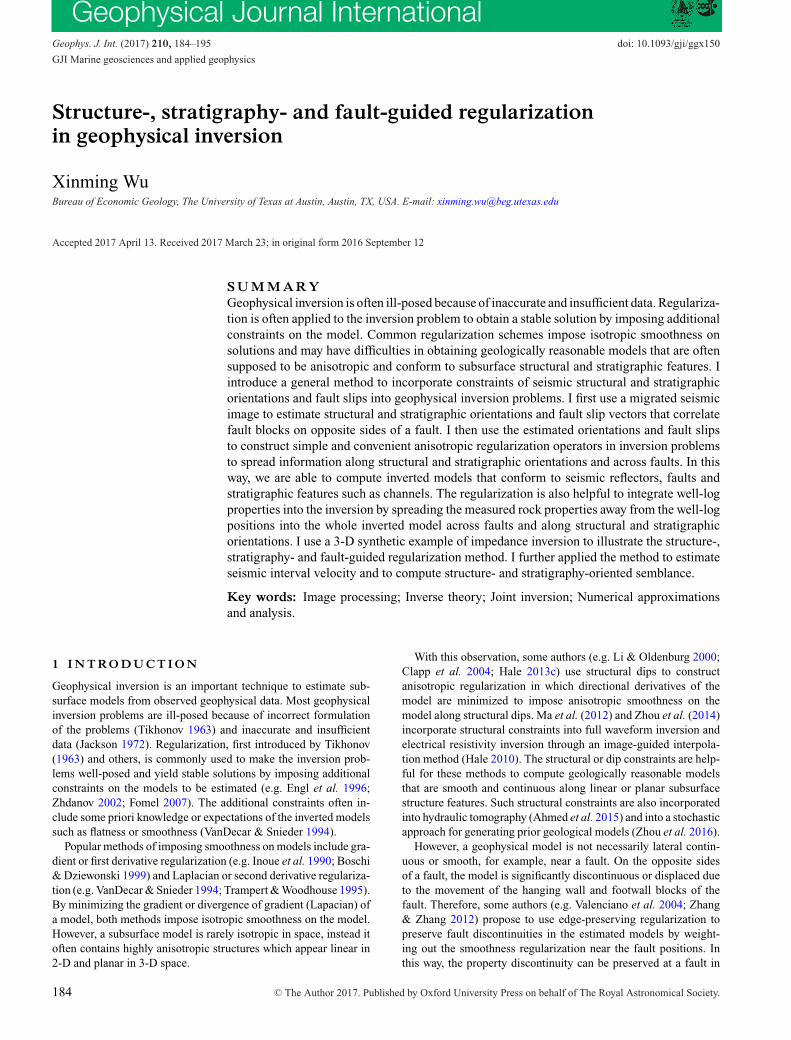
Figure 1. (a) A 3-D seismic image is displayed with a horizon surface, which is picked by following seismic reflectors. The eigenvectors (yellow segments)(b) v and (c) w of structure tensors are aligned within the horizon surface and are perpendicular and parallel to the channel, respectively. These vectors areestimated directly from the seismic image without picking the horizon.

Similarly, we label the eigenvalues and corresponding eigenvectorsso that λu ≥ λv ≥ λw .

As discussed by Hale (2009b), the eigenvectors u, correspondingto the largest eigenvalues λu, are orthogonal to linear or planarfeatures. Both eigenvectors v and w lie within the planes of anyplanar features (seismic reflections), and indicate orientations ofstratigraphic features such as channels apparent within the planes.As shown in Fig. 1(a), the horizon surface is picked following thelocally planar reflections, and a channel (denoted by cyan arrows) isapparent on the surface. The eigenvectors v and w are aligned withinthe horizon surface as denoted by the yellow segments in Figs 1(b)and (c). Near the seismic channel, we observe that eigenvectors vare orthogonal to the channel while the eigenvectors w are parallelto the channel. Away from the channel, the eigenvectors v and ware arbitrarily oriented but still aligned within the horizon surface.Although I display the eigenvectors v and w only on the extractedhorizon surface, I actually estimate the vectors for all image samplesin the 3-D seismic image. I estimate these vectors directly fromthe 3-D seismic image using structure tensors (eq. 5) without firstextracting horizon surfaces.

3 FAU LT S L I P S

Fault is another common type of geologic structure that representsdiscontinuity of subsurface rock properties. Across a fault, thereare significant displacements due to the movement of the hangingwall and footwall blocks on the opposite sides of the fault. Faultslip is defined as the displacement vector of the hanging wall blockrelative to the footwall block. Such fault slips are often spatiallyvariant along a fault surface in both fault strike and dip directions.To extend information across a fault in geophysical inversion, wehave to first estimate the fault slip vectors which tell us how tocorrelate rock properties across the fault.

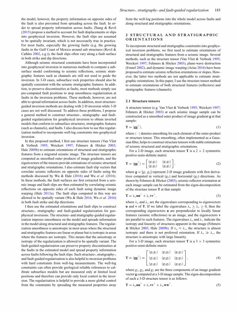
Similar to the structural and stratigraphic orientations, we canalso estimate fault slip vectors from a seismic image. In a seis-mic image, faults represent discontinuities of seismic reflectors andfault slips represent displacement vectors of the reflectors acrossthe faults. As discussed by Wu & Hale (2016), fault strike slipsare typically less apparent than dip slips in a 3-D seismic image.Therefore, we often can estimate only fault dip slips from a seismicimage. As shown in Fig. 2, fault dip slip is a displacement vector,in the dip direction, of the hanging wall side of a fault relative tothe footwall side.

To estimate fault dip slips, I first use the methods discussed byWu & Hale (2016) to extract fault surfaces (Fig. 3b) from a seismicimage (Fig. 3a). As discussed in detail by Wu & Hale (2016), I then

Figure 2. Fault dip slip is a vector representing fault displacement in thedip direction. Fault throw is the vertical component of the slip.

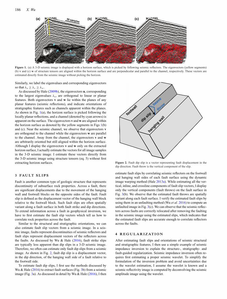
estimate fault slips by correlating seismic reflectors on the footwalland hanging wall sides of each fault surface using the dynamicimage warping method (Hale 2013a). While estimating all the ver-tical, inline, and crossline components of fault slip vectors, I displayonly the vertical components (fault throws) on the fault surface inFig. 3(b). We observe that the estimated fault throws are spatiallyvariant along each fault surface. I verify the estimated fault slips byusing them in an unfaulting method (Wu et al. 2016) to compute anunfaulted image in Fig. 3(c). We can observe that the seismic reflec-tors across faults are correctly relocated after removing the faultingin the seismic image using the estimated slips, which indicates thatthe estimated fault slips are accurate enough to correlate reflectorsacross the faults.

4 R E G U L A R I Z AT I O N

After estimating fault slips and orientations of seismic structuraland stratigraphic features, I then use a simple example of seismicimpedance inversion to explain the structure-, stratigraphy- andfault-guided regularization. Seismic impedance inversion often re-quires first estimating a proper seismic wavelet. To simplify theformulation of the inversion problem and avoid uncertainties dueto the wavelet estimation, I assume the wavelet is known and aseismic reflectivity image is computed by deconvolving the seismicamplitude image using the wavelet.

Structure-, stratigraphy- and fault-guided regularization 187

Figure 3. (a) A 3-D seismic image is displayed with (b) fault surfaces coloured by fault throws which are vertical components of estimated fault slip vectors.The fault slips are verified by using them to (c) remove the faulting in the seismic image.

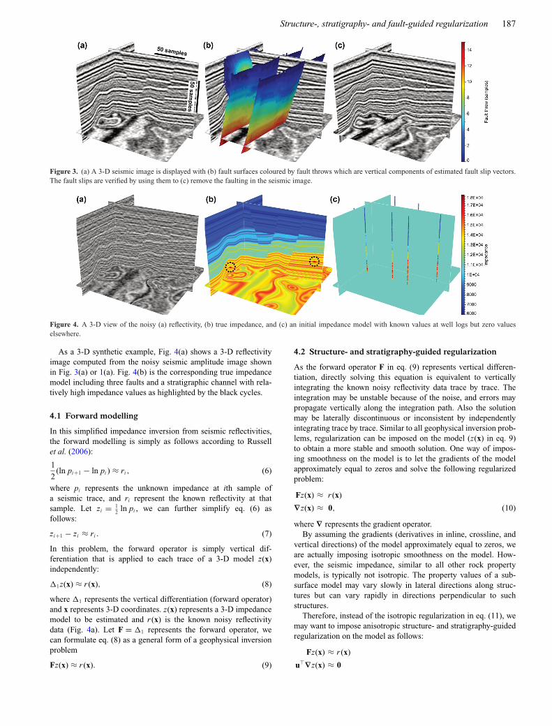
Figure 4. A 3-D view of the noisy (a) reflectivity, (b) true impedance, and (c) an initial impedance model with known values at well logs but zero valueselsewhere.

As a 3-D synthetic example, Fig. 4(a) shows a 3-D reflectivityimage computed from the noisy seismic amplitude image shownin Fig. 3(a) or 1(a). Fig. 4(b) is the corresponding true impedancemodel including three faults and a stratigraphic channel with rela-tively high impedance values as highlighted by the black cycles.

4.1 Forward modelling

In this simplified impedance inversion from seismic reflectivities,the forward modelling is simply as follows according to Russellet al. (2006):

1

2(ln pi+1 − ln pi ) ≈ ri , (6)

where pi represents the unknown impedance at ith sample ofa seismic trace, and ri represent the known reflectivity at thatsample. Let zi = 1

2 ln pi , we can further simplify eq. (6) asfollows:

zi+1 − zi ≈ ri . (7)

In this problem, the forward operator is simply vertical dif-ferentiation that is applied to each trace of a 3-D model z(x)independently:

�1z(x) ≈ r (x), (8)

where �1 represents the vertical differentiation (forward operator)and x represents 3-D coordinates. z(x) represents a 3-D impedancemodel to be estimated and r (x) is the known noisy reflectivitydata (Fig. 4a). Let F = �1 represents the forward operator, wecan formulate eq. (8) as a general form of a geophysical inversionproblem

Fz(x) ≈ r (x). (9)

4.2 Structure- and stratigraphy-guided regularization

As the forward operator F in eq. (9) represents vertical differen-tiation, directly solving this equation is equivalent to verticallyintegrating the known noisy reflectivity data trace by trace. Theintegration may be unstable because of the noise, and errors maypropagate vertically along the integration path. Also the solutionmay be laterally discontinuous or inconsistent by independentlyintegrating trace by trace. Similar to all geophysical inversion prob-lems, regularization can be imposed on the model (z(x) in eq. 9)to obtain a more stable and smooth solution. One way of impos-ing smoothness on the model is to let the gradients of the modelapproximately equal to zeros and solve the following regularizedproblem:

Fz(x) ≈ r (x)

∇z(x) ≈ 0, (10)

where ∇ represents the gradient operator.By assuming the gradients (derivatives in inline, crossline, and

vertical directions) of the model approximately equal to zeros, weare actually imposing isotropic smoothness on the model. How-ever, the seismic impedance, similar to all other rock propertymodels, is typically not isotropic. The property values of a sub-surface model may vary slowly in lateral directions along struc-tures but can vary rapidly in directions perpendicular to suchstructures.

Therefore, instead of the isotropic regularization in eq. (11), wemay want to impose anisotropic structure- and stratigraphy-guidedregularization on the model as follows:

Fz(x) ≈ r (x)

u�∇z(x) ≈ 0

188 X. Wu

v�∇z(x) ≈ 0

w�∇z(x) ≈ 0. (11)

As discussed above, u(x), v(x), and w(x) are eigenvectors com-puted from the eigen-decomposition of 3-D seismic structure ten-sors. These eigenvectors are computed for all samples x in a 3-Dseismic image. The eigenvectors u are orthogonal to linear or planarfeatures (seismic reflectors). Both eigenvectors v and w lie withinthe planes of any planar features, and indicate orientations of strati-graphic features such as channels apparent within the planes. Morespecifically, the vectors v are orthogonal to stratigraphic featuresand w are parallel to such features as shown in Figs 1(b) and (c),respectively. u�∇, v�∇, and w�∇ represent directional derivativesin directions along the vectors u, v, and w, respectively.

By setting the directional derivatives of the model to be approx-imately zeros, we are actually imposing smoothness on the modelin directions along the vectors u, v and w. We can also imposedifferent extents of smoothness on the model in different directionsby weighting the regularization terms

Fz(x) ≈ r (x)

μuu�∇z(x) ≈ 0

μvv�∇z(x) ≈ 0

μww�∇z(x) ≈ 0. (12)

These weights can be either constants or spatially variant qualitymaps. For example, a seismic impedance model, as the one shownin Fig. 4(a), varies slowly in lateral directions (v and w) alongstructures but vary rapidly in directions (u) perpendicular to thestructures. Therefore, in this case, we can set the weights μu to benearly zeros but set μv and μw with high values (close to ones).

4.3 Fault-guided regularization

With the structure- and stratigraphy-guided regularization, we areimposing smoothness on a model in directions along seismic struc-tural and stratigraphic features. However, property values of asubsurface model are not always smooth and continuous alongthe structural and stratigraphic features, they are discontinuousacross faults, like the impedance values in Fig. 4(b). One way topreserve property discontinuities at faults in a model is to first detectthe fault positions, and then set zero values at the fault positions inthe weighing maps μu, μv , and μw to stop smoothness constraintsat the faults.

In this way, we are able to preserve discontinuities at faults, butalso prevent property information on opposite sides of faults fromspreading across the faults. The property values on opposite sidesof faults are discontinuous but are correlated by fault slips vectors.Therefore, a better way of dealing with faults is to add fault slipconstrained regularization to the model as follows:

Fz(x) ≈ r (x)

μuu�∇z(x) ≈ 0

μvv�∇z(x) ≈ 0

μww�∇z(x) ≈ 0

μsβ[z(xh) − z(x f )

] ≈ 0, (13)

where μs represents a weight for the fault-guided regularizationterm and often is a constant. β is another constant scale used tobalance the fault-guided regularization with the other equations. Inmost cases, I use β = N

L , where N represents the number of sam-ples in the model while L represents the number of samples on the

faults. xh represent locations of samples adjacent to a fault from theits hanging wall side, while x f represent locations of correspondingsamples adjacent to the fault from its footwall side. Given any sam-ple xh located at the hanging wall side, we can find the correspondingcorrelated sample at the footwall side using the estimated fault slipvector s(xh) at xh : x f = xh − s(xh). This fault-guided regulariza-tion term means that we expect the model property values of thecorrelated samples on opposite sides of faults to be approximatelyequal. At the points xh and x f where the fault-guided regularizationis defined, the structure- and stratigraphy-guided regularization isturned off by setting μu = μv = μw = 0 to stop the smoothnessconstraints near the faults. Using this regularization, we are ableto spread property information across faults while preserving theproperty discontinuities at the faults. With this regularization, weassume that the rock layers across faults are geologically consistentfollowing fault slips. For some growth faults where the layers acrossfaults cannot be correlated, we might want to stop spreading prop-erty information across faults by simply setting μu = μv = μw = 0at faults.

4.4 Least-squares solution

Letting M represent the scaled differentiation operator(μsβ[z(xh) − z(x f )]) applied only to the samples adjacent to faults,we can rewrite the above eq. (13) in a simpler form as follows:

Fz(x) ≈ r (x)

μuu�∇z(x) ≈ 0

μvv�∇z(x) ≈ 0

μww�∇z(x) ≈ 0

Mz(x) ≈ 0. (14)

With the extra structure-, stratigraphy-, and fault-guided regular-ization terms, we now have more equations than unknowns as ineq. (14). Therefore, we can compute a least-squares solution ofthese equations by solving the corresponding normal equation:(

F�F + ∇�D∇ + M�M)

z(x) = F�r (x), (15)

where D = μ2uuu� + μ2

vvv� + μ2www� is an anisotropic tensor

field which has exactly the same eigenvectors as those in the 3-Dstructure tensors (eq. 5). However, the corresponding eigenvaluesare replaced with specified weights μ2

u , μ2v , and μ2

w .The above inversion with structure-, stratigraphy- and structure-

guided regularization contains three parts:

Structure-, stratigraphy- and fault-guided inversion(i): forward modelling

F�Fz(x) = F�r (x) (16)

(ii): structure- and stratigraphy-guided regularization

∇�D∇z(x) = 0 (17)

(iii): fault-guided regularization

M�Mz(x) = 0 (18)

The first part contains the forward modelling operator F. The secondpart is structure- and stratigraphy-guided regularization which sim-ply includes the gradient operator (∇) and an anisotropic tensor field(D) constructed from the eigenvector of seismic structure tensorsand some specified weights. With this tensor field, the anisotropic

Structure-, stratigraphy- and fault-guided regularization 189

smoothness constraints imposed on the model are structure- andstratigraphy-oriented. We are able to conveniently impose differentextents of the anisotropic smoothness in different orientations byvarying the corresponding weights μu, μv and μw . In most cases,we can simply set these weights to be constant values in the rangebetween 0 and 1 to specify the strength of smoothness in directionsof vectors u, v, and w. In practice, the subsurface rock propertiesoften extend more smoothly and continuously in directions parallel(vectors v and w) to structural and stratigraphic features than in di-rections perpendicular to such features. Based on this observation,we should set μu to be nearly zero while set μv and μw to be closeto one in most geophysical inversion problems to obtain subsurfacemodels conforming to structural and stratigraphic features. Theseweights μu, μv , and μw can also be set as mappings with spatiallyvariant values in the range between 0 and 1 to impose spatiallyvariant and anisotropic smoothness regularization in geophysicalinversion. In practice, such mappings can be computed as isotropyor linearity and planarity (Hale 2009b; Wu 2017) of seismic re-flections in a seismic image. In areas with lower isotropy or higherlinearity and planarity, we should set smaller μu but larger μv andμw in these areas to impose stronger smoothness in directions ofvectors v and w. In areas with higher isotropy or lower linearity andplanarity, we should set μu, μv and μw to be approximately equalto impose isotropic smoothness in these areas. More discussions ofchoosing spatially constant or variant weights will be discussed insynthetic and real examples.

The third part is the fault-guided regularization which contains asimple differentiation operator applied only to the samples adjacentto faults. By solving these three parts simultaneously as in eq. (15),we are able to obtain an inverted model conforms to faults andstructural and stratigraphic features. As the matrices in the eq. (15)are symmetric positive definite, we can solve the linear system usingthe Conjugate Gradient (CG) method.

4.5 Constraints from well logs

Geophysical inversion often also requires a starting model. A properinitial model can be helpful to reduce uncertainties in the inversionand may accelerate the convergence of the inversion process. Suchan initial model can be interpolated from well-log measurements.Hale (2009a, 2010) proposes an image-guided interpolation methodto compute a subsurface model that conforms to both seismic struc-tures and well-log measurements.

With structure-, stratigraphy-, and fault-guided regularization,we do not need to first interpolate an initial model conforms tostructures and well-log measurements. These regularization termswill spread the well-log measurements away from well positions tothe whole volume along structural and stratigraphic features andacross faults. Therefore, we can combine the initial model inter-polation and the inversion into one step by solving the followingproblem of structure-, stratigraphy- and fault-guided inversion withhard constraints from well-log measurements.

In the forth part of constraints, {fk, k = 1, 2, . . . , m} representa set of m known values which can be rock property values mea-sured in well logs. xk represent positions of the m known values. Asdiscussed previously, by solving the first three parts (i, ii and iii) si-multaneously, we compute a solution of structure-, stratigraphy- andfault-guided inversion. If we solve the second three parts (ii, iii andiv) simultaneously, we actually compute a structure-, stratigraphy-,and fault-guided interpolation of the known values. As discussedby Hale (2009a), solving the second part and the forth part simul-

Structure-, stratigraphy- and fault-guided inversion with constraints(i): forward modelling

F�Fz(x) = F�r (x) (19)

(ii): structure- and stratigraphy-guided regularization

∇�D∇z(x) = 0 (20)

(iii): fault-guided regularization

M�Mz(x) = 0 (21)

(iv): hard constraints

subject to z(xk ) = fk , k = 1, 2, . . . , m (22)

taneously yields an image-guided harmonic interpolation. With theconstraint equation (the forth part), we expect the interpolant z(x)to be equal to the known values z(xk) = fk at the know positions xk .With the equation of structural and stratigraphic regularization (sec-ond part), we expect the directional derivatives of the interpolantz(x) in structural and stratigraphic orientations to be approximatelyzeros. Solving these two equations simultaneously, we are able toextend the known values smoothly along the structural and strati-graphic orientations to compute a structure- and stratigraphy-guidedinterpolation.

The constraints of known properties often can only provide localcontrol in the inversion because those properties are often measuredonly at limited positions. The structure-, stratigraphy-, and fault-guided regularization is helpful to provide a more global control byspreading the measured properties across faults and along structuraland stratigraphic features. By combining all the above four parttogether, we solve a following constrained linear system:(

F�F + ∇�D∇ + M�M)

z(x) = F�r (x)

subject to z(xk) = fk, k = 1, 2, . . . , m. (23)

This constrained linear system combines the interpolation and theinversion, both of which are guided by fault slips and structural andstratigraphic orientations.

I solve this constrained linear system using a preconditionedCG method (Wu & Hale 2015; Wu et al. 2016). The constraintequation z(xk) = fk, k = 1, 2, . . . , m is implemented with simplepre-conditioners in the CG method; the details of constructing suchpre-conditioners are discussed by Wu & Hale (2015). In this precon-ditioned CG method, I choose a simple initial model with zero valueseverywhere but known values fk at xk , which obviously satisfies theconstraint equation. Beginning with such an initial model that satis-fies the constraint equation, the CG iterations gradually update thefunction for all samples, while the pre-conditioners guarantee thatthe updated function always satisfies the constraint equation aftereach iteration.

4.6 Results

Fig. 4 shows the 3-D synthetic example I use to illustrate the reg-ularization and the hard constraints from well logs. This examplecontains three faults (Fig. 3b) and a channel with relatively highimpedance values as denoted by black circles in the true impedancemodel (Fig. 4b). Fig. 4(a) shows a noisy reflectivity image computedby devolving the corresponding seismic image (Figs 1a and 3a)with a known wavelet. The goal of this example is to invert animpedance model from this noisy reflectivity image with constraintsof the known impedance values recorded at the 7 well logs shownin Fig. 4(c).

190 X. Wu

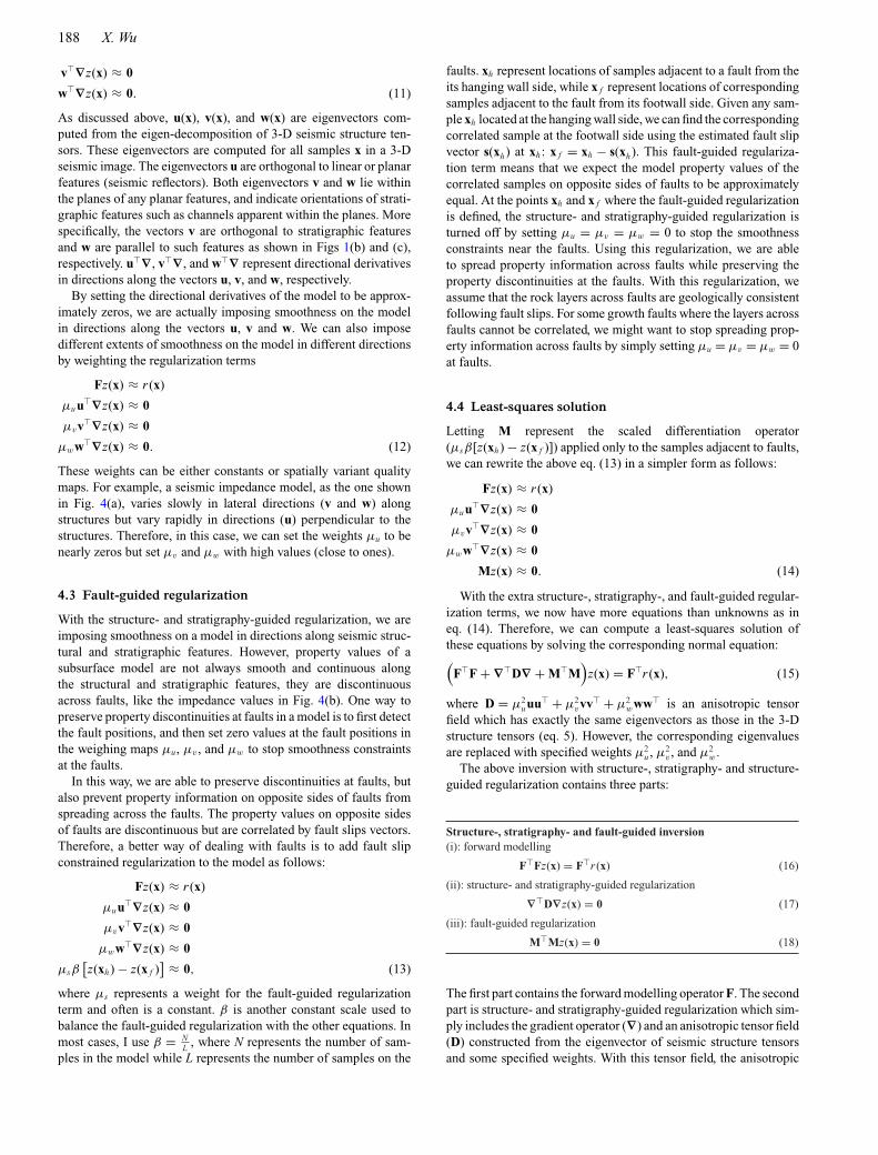
Figure 5. (a) Estimated impedance model with μu = 0.001 and μv = μw = μs = 0.1. (b) Estimated impedance model with μu = 0.001, μv = μw = 0.9, andμs = 0.0. (c) Estimated impedance model with μu = 0.001 and μv = μw = μs = 0.9.

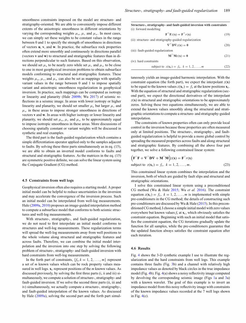
Figure 6. (a) True impedance model. (b) Estimated impedance model with μu = 0.001 and μv = μw = μs = 0.9. (c) Estimated impedance model withμu = 0.001, μv = 0.01 and μw = μs = 0.9. The channel (denoted by cyan arrows) with relatively high impedance values is smoothed out in (b) but is preservedin (c).

In this example, I first estimate structural and stratigraphic ori-entations from the seismic image (Figs 1a and 3a) using structuretensors (eq. 5). From the eigen-decomposition of the structure ten-sors, I obtain three eigenvectors u, v, and w with correspondingthree eigenvalues λu ≥ λv ≥ λw . As discussed previously in thispaper, the eigenvectors u are orthogonal to linear or planar features.Both eigenvectors v and w lie within the planes of any planar fea-tures (seismic reflections), and indicate orientations of stratigraphicfeatures such as channels apparent within the planes. As shown inFigs 1(b) and (c), the vectors v and w are aligned within the hori-zon surface which is extracted following seismic reflectors. More-over, vectors v (Fig. 1b) are orthogonal to channel and w (Fig. 1c)are parallel to the channel. In areas without stratigraphic features,the image features on the horizon surface are isotropic and theeigenvectors v and w are arbitrarily oriented as shown in Figs 1(b)and (c).

I also extract fault surfaces from the 3-D seismic image (Fig. 3b)and estimate fault slips on the surfaces. Fault slips are vectors withinline, crossline, and vertical components. I display only the verticalcomponents (fault throws) on the fault surfaces shown in Fig. 3(b).To verify the estimated faults slip vectors, I use them to removethe faulting the original seismic image (Fig. 3a) and obtain anunfaulted image (Fig. 3c). In this unfaulted image, seismic reflectorsare relocated across faults, which indicates that the estimated faultslips are accurate enough to correlate seismic reflectors across thefaults.

With the estimated structural and stratigraphic orientations (u, vand w) and the fault slip vectors (s(xh)), I construct regularizationterms as in eq. (13) for the seismic impedance inversion. In general,a impedance model varies slowly along structural and stratigraphicfeatures in directions along the vectors v, and w but likely variesrapidly in directions along the vectors u which are perpendicular

to such features. Therefore, when constructing regularization forimposing smoothness on the model, I set μu = 0.001 to imposeweak smoothness in the directions of vectors u for all tests (Figs 5and 6) in this 3-D synthetic example.

In all these tests shown in Figs 5 and 6, I begin with an initialimpedance model with known values at well-log positions and zerovalues elsewhere and solve the constrained linear system (eq. 23)using a preconditioned CG method. However, for each test, I setdifferent weights μv , μw and μs in constructing the regularizationterms ∇�D∇ and M�M in eq. (23).

In computing the impedance model shown in Fig. 5(a), I setμv = μw = μs = 0.1 which means that I impose weak smoothnesson the model in all directions along structural and stratigraphicfeatures and across faults. We observe that the estimated impedancemodel (Fig. 5a) is noisy because of the noisy input reflectivity data(Fig. 4a).

In computing the impedance model shown in Fig. 5(b), I setμv = μw = 0.9 and μs = 0.0 which means that I impose strongsmoothness on the model in directions along structures but imposeno constraints on the model across faults. With these settings for theregularization, I obtain a much cleaner impedance model (Fig. 5b)with more continuous values along structures comparing to theestimated model with weaker smoothness regularization (Fig. 5a).However, if we compare this estimated model (Fig. 5b) with thetrue impedance model (Fig. 4b), we observe that the discontinuitiesat the fault positions are not preserved because of the smoothnessregularization along structures.

In computing the impedance model shown in Fig. 5(c), I setμv = μw = μs = 0.9 which means that I impose strong smoothnesson the model in directions along structures and also impose strongfault-guided regularization on the model across faults. With allthese regularization, I obtain an estimated model (Fig. 5c) which

Structure-, stratigraphy- and fault-guided regularization 191

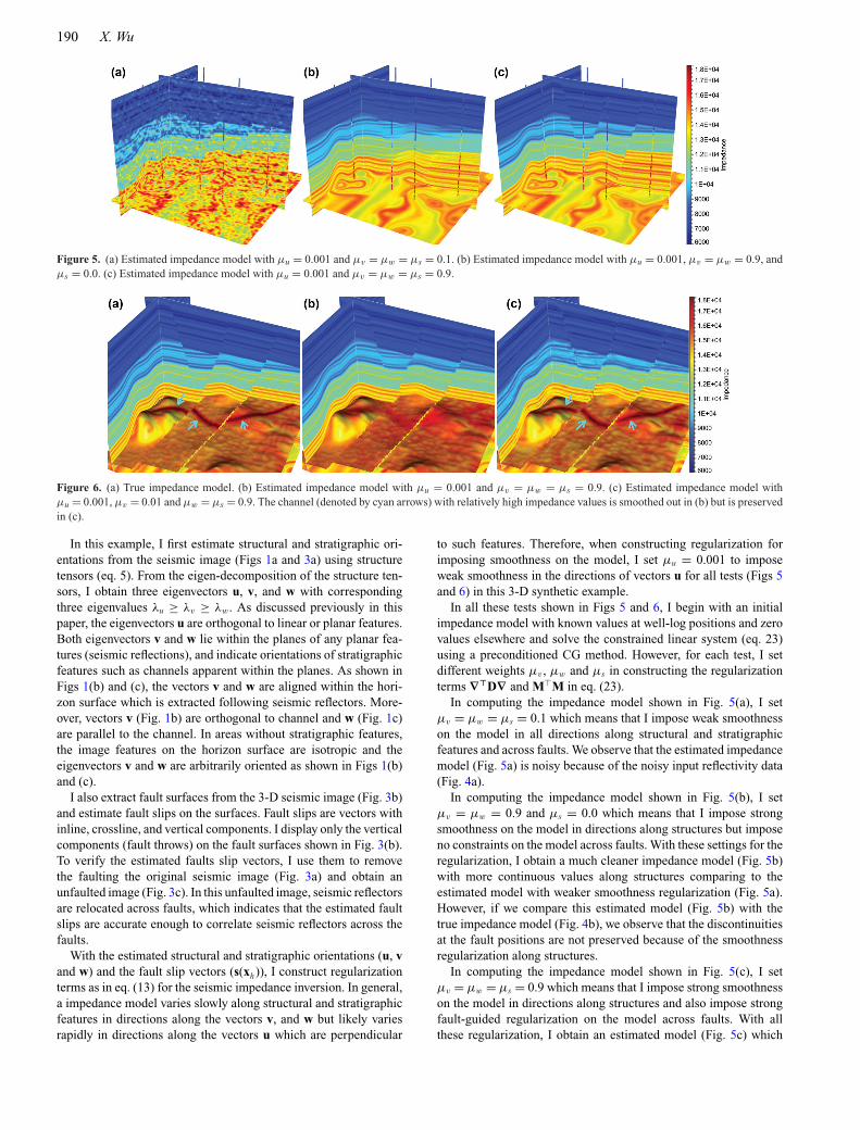
Figure 7. (a) 2-D time-migrated image. (b) The corresponding migrationvelocity from automatic picking. Both of the images are reproduced fromthe paper published by Fomel (2007).

is smooth and continuous along structures but discontinuous atfaults, as expected. This estimated model is visually close to thetrue impedance model shown in Fig. 4(b). However, one problem ofthis estimated model is that the stratigraphic features (channel) aresmoothed out as shown in Fig. 6(b) because of the strong smoothnessregularization along directions of vectors v which are orthogonal tothe stratigraphic features.

Therefore, in computing the impedance model shown in Fig. 6(c),I set μv = 0.01 and μw = μs = 0.9 to impose strong regularizationon the model only in directions along stratigraphic features andacross faults. By doing this, we decrease the smoothness constraintson the model in directions orthogonal to channel and thereforepreserve the relatively high impedance values on the channel asshown in Fig. 6(c). In this synthetic example, I directly use the well-log impedances as constraints to compute an impedance model. Inpractice, we might want to use only the low-frequency componentsof the well-log impedances as constraints in seismic impedanceinversion to compensate the missing low frequencies in seismic data.

5 R E A L E X A M P L E S

Although the structure-, stratigraphy-, and fault-guided regulariza-tion is derived with the example of seismic impedance inversion, thisregularization can be applied to other geophysical inversion prob-lems. Below I use the regularization discussed above to estimateseismic interval velocity and compute structure- and stratigraphy-oriented semblance.

5.1 Velocity estimation

The first example is an application of structure- and fault-guidedregularization in seismic velocity estimation. Fig. 7(a) shows a time-migrated seismic image of historic Gulf Mexico data set that Ireproduce from the paper published by Fomel (2007). The corre-sponding migration velocity (Fig. 7b) is automatically picked fromsemblance gathers obtained in the process of velocity continuation(Fomel 2007). Again this velocity image is also reproduced fromthe paper published by Fomel (2007). The goal of this example is toestimate interval velocity from this picked time-migration velocity.

Figure 8. (a) Estimated interval velocity using shaping regularization withtriangle local plane-wave smoothing. (b) Predicted migration velocity com-puted from the estimated interval velocity. Both the results are reproducedfrom the paper published by Fomel (2007).

The picked time-migration (or root-mean-square) velocity andthe interval velocity at each trace are related as follows accordingto Dix (1955)

C2(τ ) = 1

τ

∑i

c2i �τi , (24)

where C(τ ) is the picked time-migration velocity (Fig. 7b), ci isthe interval velocity at each time sample, and τ is the verticaltraveltime. Estimating the interval velocity from the time-migrationvelocity can be stated as computing a least-squares solution of thefollowing equation (Valenciano et al. 2004)

WSc ≈ Wd, (25)

where c is the unknown vector of squared interval velocities, d isthe known vector of squared time-migration velocities multiplied bythe vertical traveltime, S is the causal integration operator, and Wis a weighing matrix constructed from the confidence of the pickedtime-migration velocities.

To obtain an interval velocity image conforms to seismic struc-tures, Fomel (2007) solve the above inversion problem (eq. 25) usingthe shaping regularization with triangle local plane-wave smooth-ing. Fig. 8(a) shows the estimated interval velocity image wheresome of the velocities do not truly follow the seismic structures.Moreover, the estimated interval velocity is smooth across faultswhere the velocity is expected to be discontinuous. Fig. 8(b) is thepredicted migration velocity computed from the estimated intervalvelocity (Fig. 8a).

Next, I solve the same inversion problem but with structure-and fault-guided regularization discussed previously in this paper.From the seismic image (Fig. 7a), I first construct a tensor fieldD(x) = μ2

uu�u + μ2vv�v for the regularization ∇�D∇ using eigen-

values and eigenvectors of 2-D structure tensors (eq. 1). Instead ofusing constant weights μu and μv as in the previous 3-D syntheticexample, in this example I define spatially variant weights usingthe spatially variant eigenvalues λu(x) and λv(x) (λu(x) ≥ λv(x)) asfollows:

μu(x) = λmin + ε0

λv(x) + ε0, and μv(x) = λmin + ε0

λu(x) + ε0, (26)

where λmin is the minimum of the eigenvalues λv(x): λmin =min

x{λv(x)}. The parameter ε0 is a small positive number used to

192 X. Wu

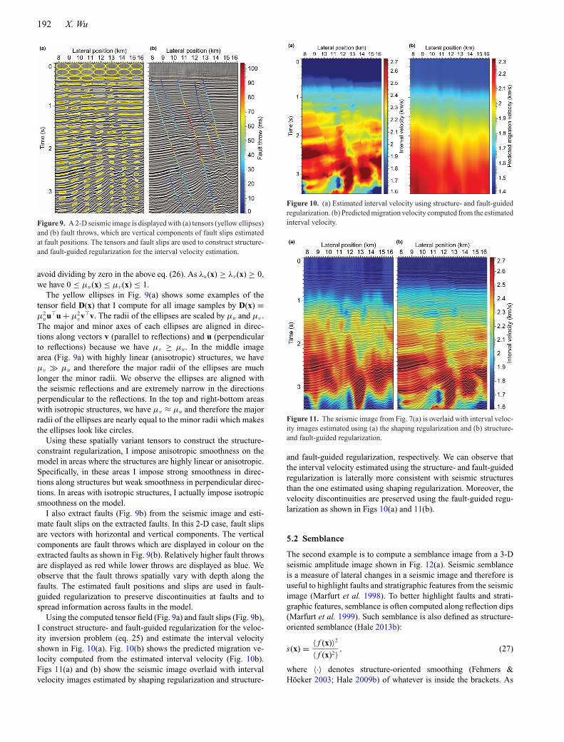
Figure 9. A 2-D seismic image is displayed with (a) tensors (yellow ellipses)and (b) fault throws, which are vertical components of fault slips estimatedat fault positions. The tensors and fault slips are used to construct structure-and fault-guided regularization for the interval velocity estimation.

avoid dividing by zero in the above eq. (26). As λu(x) ≥ λv(x) ≥ 0,we have 0 ≤ μu(x) ≤ μv(x) ≤ 1.

The yellow ellipses in Fig. 9(a) shows some examples of thetensor field D(x) that I compute for all image samples by D(x) =μ2

uu�u + μ2vv�v. The radii of the ellipses are scaled by μu and μv .

The major and minor axes of each ellipses are aligned in direc-tions along vectors v (parallel to reflections) and u (perpendicularto reflections) because we have μv ≥ μu. In the middle imagearea (Fig. 9a) with highly linear (anisotropic) structures, we haveμv � μu and therefore the major radii of the ellipses are muchlonger the minor radii. We observe the ellipses are aligned withthe seismic reflections and are extremely narrow in the directionsperpendicular to the reflections. In the top and right-bottom areaswith isotropic structures, we have μv ≈ μu and therefore the majorradii of the ellipses are nearly equal to the minor radii which makesthe ellipses look like circles.

Using these spatially variant tensors to construct the structure-constraint regularization, I impose anisotropic smoothness on themodel in areas where the structures are highly linear or anisotropic.Specifically, in these areas I impose strong smoothness in direc-tions along structures but weak smoothness in perpendicular direc-tions. In areas with isotropic structures, I actually impose isotropicsmoothness on the model.

I also extract faults (Fig. 9b) from the seismic image and esti-mate fault slips on the extracted faults. In this 2-D case, fault slipsare vectors with horizontal and vertical components. The verticalcomponents are fault throws which are displayed in colour on theextracted faults as shown in Fig. 9(b). Relatively higher fault throwsare displayed as red while lower throws are displayed as blue. Weobserve that the fault throws spatially vary with depth along thefaults. The estimated fault positions and slips are used in fault-guided regularization to preserve discontinuities at faults and tospread information across faults in the model.

Using the computed tensor field (Fig. 9a) and fault slips (Fig. 9b),I construct structure- and fault-guided regularization for the veloc-ity inversion problem (eq. 25) and estimate the interval velocityshown in Fig. 10(a). Fig. 10(b) shows the predicted migration ve-locity computed from the estimated interval velocity (Fig. 10b).Figs 11(a) and (b) show the seismic image overlaid with intervalvelocity images estimated by shaping regularization and structure-

Figure 10. (a) Estimated interval velocity using structure- and fault-guidedregularization. (b) Predicted migration velocity computed from the estimatedinterval velocity.

Figure 11. The seismic image from Fig. 7(a) is overlaid with interval veloc-ity images estimated using (a) the shaping regularization and (b) structure-and fault-guided regularization.

and fault-guided regularization, respectively. We can observe thatthe interval velocity estimated using the structure- and fault-guidedregularization is laterally more consistent with seismic structuresthan the one estimated using shaping regularization. Moreover, thevelocity discontinuities are preserved using the fault-guided regu-larization as shown in Figs 10(a) and 11(b).

5.2 Semblance

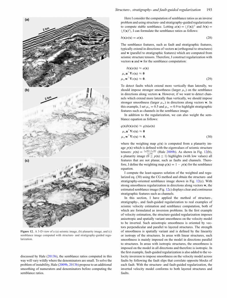
The second example is to compute a semblance image from a 3-Dseismic amplitude image shown in Fig. 12(a). Seismic semblanceis a measure of lateral changes in a seismic image and therefore isuseful to highlight faults and stratigraphic features from the seismicimage (Marfurt et al. 1998). To better highlight faults and strati-graphic features, semblance is often computed along reflection dips(Marfurt et al. 1999). Such semblance is also defined as structure-oriented semblance (Hale 2013b):

s(x) = 〈 f (x)〉2

〈 f (x)2〉 , (27)

where 〈·〉 denotes structure-oriented smoothing (Fehmers &Hocker 2003; Hale 2009b) of whatever is inside the brackets. As

Structure-, stratigraphy- and fault-guided regularization 193

Figure 12. A 3-D view of a (a) seismic image, (b) planarity image, and (c)semblance image computed with structure- and stratigraphy-guided regu-larization.

discussed by Hale (2013b), the semblance ratios computed in thisway will vary wildly where the denominators are small. To solve theproblem of instability, Hale (2009b, 2013b) propose to an additionalsmoothing of numerators and denominators before computing thesemblance ratios.

Here I consider the computation of semblance ratios as an inverseproblem and using structure- and stratigraphy-guided regularizationto compute stable semblance. Letting a(x) = 〈 f (x)〉2 and b(x) =〈 f (x)2〉, I can formulate the semblance ratios as follows:

b(x)s(x) = a(x). (28)

The semblance features, such as fault and stratigraphic features,typically extend in directions of vectors u (orthogonal to structures)and w (parallel to stratigraphic features) which are computed fromseismic structure tensors. Therefore, I construct regularization withvectors u and w for the semblance computation:

b(x)s(x) ≈ a(x)

μuu�∇s(x) ≈ 0

μww�∇s(x) ≈ 0. (29)

To detect faults which extend more vertically than laterally, weshould impose stronger smoothness (larger μu) on the semblancein directions along vectors u. However, if we want to detect chan-nels which extend more laterally than vertically, we should imposestronger smoothness (larger μw) in directions along vectors w. Inthis example, I set μu = 0.5 and μw = 0.9 to highlight stratigraphicfeatures such as channels in the semblance image.

In addition to the regularization, we can also weight the sem-blance equation as follows:

q(x)b(x)s(x) ≈ q(x)a(x)

μuu�∇s(x) ≈ 0

μww�∇s(x) ≈ 0, (30)

where the weighing map q(x) is computed from a planarity im-age p(x) which is defined with the eigenvalues of seismic structuretensors: p(x) = λu (x)−λv (x)

λu (x) (Hale 2009b). As shown in Fig. 12(b),a planarity image (0 ≤ p(x) ≤ 1) highlights (with low values) allfeatures that are not planar, such as faults and channels. There-fore, I define the weighting map q(x) = 1 − p(x) for the semblanceequation.

I compute the least-squares solution of the weighted and regu-larized eq. (30) using the CG method and obtain the structure- andstratigraphy-oriented semblance image shown in Fig. 12(c). Withstrong smoothness regularization in directions along vectors w, theestimated semblance image (Fig. 12c) displays clear and continuousstratigraphic features such as channels.

In this section, I have applied the method of structure-,stratigraphy-, and fault-guided regularization to real examples ofseismic velocity estimation and semblance computation, both ofwhich are formulated as inversion problems. In the first exampleof velocity estimation, the structure-guided regularization imposesanisotropic and spatially variant smoothness on the velocity modelto be inverted. Such anisotropic smoothness is oriented by vec-tors perpendicular and parallel to layered structures. The strengthof smoothness is spatially variant and is defined by the linearityor isotropy of the structures. In areas with linear structures, suchsmoothness is mainly imposed on the model in directions parallelto structures. In areas with isotropic structures, the smoothness isimposed on the model in all directions and therefore is isotropic. Inthe first example, fault-guided regularization is also added to the ve-locity inversion to impose smoothness on the velocity model acrossfaults by following the fault slips that correlate opposite blocks ofeach fault. With the structure- and fault-guided regularization, theinverted velocity model conforms to both layered structures andfaults.

194 X. Wu

In the second example, I formulate the computation of 3-D seis-mic semblance as a simple inversion problem, instead of directlycomputing the semblance ratios. With this formulation, we are ableto avoid obtaining wildly varying semblance due to dividing smalldenominators in computing the semblance ratios. In addition, wecan also add structure- and stratigraphy-guided regularization tothe inversion formulation of semblance. In this example of detect-ing seismic channels, I set μv = 0 in the regularization because wedo not expect to impose smoothness on the semblance in directionslaterally perpendicular to the channels, which will blur the channelfeatures in a semblance image. In addition, channels often extendlaterally longer along vectors w than vertically along vectors u.Therefore, I impose stronger smoothness laterally along w than ver-tical along u (μw = 0.9, μv = 0.5) in the regularization to enhancechannel features in the semblance image. If we want to compute asemblance image for fault detection, we should impose smoothnessin directions along both the fault strike and dip directions to enhancefault features in the semblance image.

6 C O N C LU S I O N S

I have introduced a general scheme to construct convenientstructure-, stratigraphy- and fault-guided regularization for geo-physical inversion to estimate models that conform to seismic faults,reflectors, and seismic stratigraphic features such as channels.

The regularization requires first estimating structural and strati-graphic orientations and fault slip vectors from a migrated seismicimage. The structure- and stratigraphy-guided regularization im-poses smoothness on the inverted model along the orientations ofstructural and stratigraphic features such as seismic reflections andchannels. Such regularization is often anisotropic in most areas butcan be isotropic in areas where the structural and stratigraphic fea-tures are isotropic, which means that the anisotropy or isotropy ofthe regularization can be spatially variant. The fault-guided regu-larization, constructed with fault slips, preserves discontinuities atfaults and spreads information across faults in the inverted model.

The regularization is especially helpful for inversion with con-straints from well-log properties or other geophysical measure-ments. Such constraints are often limited to only local positionsand therefore may have difficulties in providing global control inthe inversion. The regularization is helpful to extend the controlof the constraints by spreading the properties from the measuredpositions into the whole inverted model across faults and alongstructural and stratigraphic orientations.

In all examples discussed in this paper, I assume the propertiesof the estimated models are consistent with seismic structures andstratigraphic features, which is not necessarily true for some othermodels. However, we can conveniently vary the regularization fordifferent applications with proper weights (μu(x), μv(x) and μw(x)in eq. 14) to produce desired features in the inverted model. Forexample, we might want to use different kinds of seismic attributesthat highlight reservoirs or discontinuities of subsurface models asweights to construct the regularization.

A C K N OW L E D G E M E N T S

The idea of structure-oriented regularization discussed in this paperis originally from an enlightening talk ‘Structure-oriented Process-ing and Inversion’ given by Dr Dave Hale in the 2013 sponsor meet-ing of the Center for Wave Phenomena. I thank Dr Sergey Fomeland Dr Junzhe Sun for inspiring discussions. The seismic image of

buried channels is a subset of the Parihaka 3-D data set providedby New Zealand Crown Minerals through the SEG Wiki website(http://wiki.seg.org/wiki/Parihaka-3D). This research is supportedby the sponsors of the Texas Consortium for Computational Seis-mology (TCCS).

R E F E R E N C E S

Ahmed, A.S., Zhou, J., Jardani, A., Revil, A. & Dupont, J., 2015. Image-guided inversion in steady-state hydraulic tomography, Adv. Water Re-sour., 82, 83–97.

Arias, E., 2016. Estimating seismic reflection slopes, Master’s thesis, Col-orado School of Mines.

Boschi, L. & Dziewonski, A.M., 1999. High-and low-resolution images ofthe earth’s mantle: implications of different approaches to tomographicmodeling, J. geophys. Res., 104(B11), 25 567–25 594.

Clapp, R.G., Biondi, B.L. & Claerbout, J.F., 2004. Incorporating geologicinformation into reflection tomography, Geophysics, 69(2), 533–546.

Dix, C.H., 1955. Seismic velocities from surface measurements, Geophysics,20(1), 68–86.

Engl, H.W., Hanke, M. & Neubauer, A., 1996. Regularization of InverseProblems, Springer Science & Business Media.

Fehmers, G.C. & Hocker, C.F., 2003. Fast structural interpretation withstructure-oriented filtering, Geophysics, 68(4), 1286–1293.

Fomel, S., 2002. Applications of plane-wave destruction filters, Geophysics,67(6), 1946–1960.

Fomel, S., 2007. Shaping regularization in geophysical-estimation problems,Geophysics, 72(2), R29–R36.

Hale, D., 2009a. Image-guided blended neighbor interpolation of scattereddata, in 79th Annual International Meeting, SEG, Expanded Abstracts,pp. 1127–1131.

Hale, D., 2009b. Structure-oriented smoothing and semblance, CWP Report635.

Hale, D., 2010. Image-guided 3D interpolation of borehole data, in 80thAnnual International Meeting, SEG, Expanded Abstracts, pp. 1266–1270.

Hale, D., 2013a. Dynamic warping of seismic images, Geophysics, 78,S105–S115.

Hale, D., 2013b. Methods to compute fault images, extract fault surfaces,and estimate fault throws from 3D seismic images, Geophysics, 78(2),O33–O43.

Hale, D., 2013c. Structure-oriented processing and inversion, in 2013 ProjectReview meeting of the Consortium Project on Seismic Inverse Methodsfor Complex Structures, Colorado School of Mines, Golden, US.

Inoue, H., Fukao, Y., Tanabe, K. & Ogata, Y., 1990. Whole mantle P-wavetravel time tomography, Phys. Earth planet. Inter., 59(4), 294–328.

Jackson, D.D., 1972. Interpretation of inaccurate, insufficient and inconsis-tent data, Geophys. J. Int., 28(2), 97–109.

Li, Y. & Oldenburg, D.W., 2000. Incorporating geological dip informationinto geophysical inversions, Geophysics, 65(1), 148–157.

Ma, Y., Hale, D., Gong, B. & Meng, Z.J., 2012. Image-guided sparse-modelfull waveform inversion, Geophysics, 77(4), R189–R198.

Marfurt, K.J., Kirlin, R.L., Farmer, S.L. & Bahorich, M.S., 1998. 3-D seis-mic attributes using a semblance-based coherency algorithm, Geophysics,63(4), 1150–1165.

Marfurt, K.J., Sudhaker, V., Gersztenkorn, A., Crawford, K.D. & Nissen,S.E., 1999. Coherency calculations in the presence of structural dip, Geo-physics, 64(1), 104–111.

Revil, A. & Cathles, L., 2002. Fluid transport by solitary waves alonggrowing faults: a field example from the South Eugene Island Basin, Gulfof Mexico, Earth planet. Sci. Lett., 202(2), 321–335.

Russell, B., Hampson, D. & Bankhead, B., 2006. An inversion primer, CSEGRecorder, 31, 96–102.

Tikhonov, A., 1963. Solution of incorrectly formulated problems and theregularization method, Sov. Math. Dokl., 5, 1035–1038.

Trampert, J. & Woodhouse, J.H., 1995. Global phase velocity maps of Loveand Rayleigh waves between 40 and 150 seconds, Geophys. J. Int., 122(2),675–690.

Structure-, stratigraphy- and fault-guided regularization 195

Valenciano, A.A., Brown, M. & Guitton, A., 2004. Interval veloc-ity estimation using edge-preserving regularization, in 74th An-nual International Meeting, SEG, Expanded Abstracts, pp. 2431–2434.

Van Vliet, L.J. & Verbeek, P.W., 1995. Estimators for orientation andanisotropy in digitized images, in Proceedings of the first annual con-ference of the Advanced School for Computing and Imaging ASCI’95,Heijen, The Netherlands, pp. 442–450.

VanDecar, J.C. & Snieder, R., 1994. Obtaining smooth solutions to large,linear, inverse problems, Geophysics, 59(5), 818–829.

Weickert, J., 1997. A review of nonlinear diffusion filtering, in Scale-SpaceTheory in Computer Vision, vol. 1252 of Lecture Notes in ComputerScience, pp. 1–28, eds ter Haar Romeny, B., Florack, L., Koenderink, J.& Viergever, M., Springer.

Wu, X., 2017. Directional structure-tensor based coherence to detect seismicfaults and channels, Geophysics, 82(2), A13–A17.

Wu, X. & Hale, D., 2015. Horizon volumes with interpreted constraints,Geophysics, 80, IM21–IM33.

Wu, X. & Hale, D., 2016. 3D seismic image processing for faults, Geo-physics, 81(2), IM1–IM11.

Wu, X., Luo, S. & Hale, D., 2016. Moving faults while unfaulting 3D seismicimages, Geophysics, 81(2), IM25–IM33.

Zhang, J. & Revil, A., 2015. 2d joint inversion of geophysical data usingpetrophysical clustering and facies deformation, Geophysics, 80(5), M69–M88.

Zhang, X. & Zhang, J., 2012. Edge preserving regularization for seismictraveltime tomography, in 82nd Annual International Meeting, SEG, Ex-panded Abstracts, pp. 1–5.

Zhdanov, M., 2002. Geophysical Inverse Theory and Regularization Prob-lems, Elsevier Science.

Zhou, J., Revil, A., Karaoulis, M., Hale, D., Doetsch, J. & Cuttler, S., 2014.Image-guided inversion of electrical resistivity data, Geophys. J. Int., 197,292–309.

Zhou, J., Revil, A. & Jardani, A., 2016. Stochastic structure-constrainedimage-guided inversion of geophysical data, Geophysics, 81(2), E89–E101.