Structured Finance and Correlation Risk

Structured Finance and Correlation Risk∗

Marc Chesney† Felix Fattinger‡ Jonathan Krakow§

December, 2019

Abstract

We study the relation between the inherent complexity of structured products and theirendogenous issuer margins. First, using a sample of 4,460 yield enhancement products(YEP), we document a shift towards more complex payoff structures. Margins for morecomplex products are twice as high relative to their less complex counterparts, whilethe former’s realized investor returns are lower and negative on average. We identifyuncompensated correlation risk as the main mechanism behind this discrepancy. Sec-ond, we conduct a laboratory experiment to measure individuals willingness-to-pay forYEPs with varying levels of complexity. Our experimental findings provide a micro-foundation for our field results. We find that subjects systematically underestimate theembedded correlation risk of more complex products. The resulting relative overpricingis increasing in the underlying volatility and in subjects’ overconfidence. Moreover, thewillingness to invest in structured products is higher when the risk-free rate is low. Inthe face of unprecedented low interest rates and a rising popularity of YEPs, we arguethat our findings are of direct policy relevance.

Keywords : Financial innovation; structured products; product margins; correlation risk

∗We are grateful for comments from Francesco d’Acunto, Bjorn Bartling, Thorsten Hens, Steven Ongena,Per Ostberg, Alexander Wagner, Daxeng Xiu, Alexander Ziegler, and seminar participants at the Universityof Zurich, University of Melbourne, and the RBFC 2018 Conference on Behavioral Finance (Amsterdam).Jonathan Krakow acknowledges financial support from the Forschungskredit of the University of Zurich grantno. [FK-17-015].†Department of Banking and Finance, Competence Center in Sustainable Finance, University of Zurich,

Plattenstrasse 32, 8032 Zurich, Switzerland. Email: [email protected]‡Department of Finance, University of Melbourne, 198 Berkeley Street, Victoria 3053, Australia. Email:

[email protected]§Department of Banking and Finance, University of Zurich, Plattenstrasse 32, 8032 Zurich, Switzerland.

Email: [email protected]

Electronic copy available at: https://ssrn.com/abstract=3499660

[email protected]

1. Introduction

During the unprecedented period of low interest rates following the Great Recession,

the search for low-risk investments with positive yields has become increasingly difficult.

Traditionally, financial innovation is considered to arise in response to and for the benefit of

previously unmet investor needs (Allen and Gale, 1994; Duffie and Rahi, 1995). However,

there has been an ongoing debate (Zingales, 2015) and recent evidence (see, e.g., Celerier and

Vallee, 2017) about financial institutions’ strategic exploitation of information asymmetries

when catering new financial products to yield-seeking retail investors.

In response to the consistently low interest rates, a particular class of retail structured

notes has enjoyed great popularity lately among retail investors: yield enhancement products

(YEP). Combining a fixed rate bond with a short put option, YEPs promise high coupons

(headline rates), while exposing investors to the risk of potentially unlimited losses. In

Europe, where structured notes have been routinely sold to retail investors since the 1990s,

the total amount of such products held by EU households amounted to EUR 500bn in

2017–the vast majority of which (74%) excluding any capital protection.1 In the US, YEPs

represent the largest and fastest growing class of retail structured notes with more than USD

100bn sold since 2008 (Vokata, 2018).

In this paper, we investigate the demand and supply effects behind one of the most

popular types of YEPs, so-called reverse convertible notes. Reverse convertibles are com-

monly considered synonymous with structured products (Egan, 2019). Already in 2011, the

SEC referred to reverse convertibles as “perhaps the riskiest [structured securities products]

available to retail investors”, emphasizing the risk stemming from the embedded short put

option.2 Effectively, the short put option converts the product’s notional into a predefined

1See the European Securities and Markets Authority (ESMA) report on “Trends, Risks and Vulnera-bilities”, No. 2, 2018, available via https://www.esma.europa.eu/press-news/esma-news (ESMA, 2018). Asnon-EU member country, Switzerland is excluded from these statistics.

2See p. 4 of the SEC report entitled “Staff Summary Report on Issues Identified in Examina-tions of Certain Structured Securities Products Sold to Retail Investors”, July 27, 2011, available viahttps://www.sec.gov/news/studies/2011/ssp-study.pdf (SEC, 2011).

2


number of stocks, whenever the underlying asset price falls and remains below a certain

threshold. The crucial and highly non-trivial question then of course is, does the product’s

fixed coupon sufficiently compensate for its downside risk?

Our data sample spans 4,460 barrier reverse convertibles (BRC) on US equities issued in

Switzerland between 2008 and 2017. BRCs represent the vast majority of reverse convertibles

sold in Switzerland, where—in contrast to standard convertibles—the term “barrier” refers

to the barrier characteristic of the embedded put option (see Section 2.1 for details). Given

its sheer size and maturity, the Swiss market constitutes the ideal laboratory to study the

demand and supply dynamics for retail structured products. During the years of low interest

rates following the Great Recession, Switzerland has become one of the biggest markets in

the world, with outstanding volumes in YEPs reaching CHF 74bn in the first quarter of

2019.3

Our analysis proceeds in two steps. In the first part of the paper, we document that, in

recent years, the market for BRCs has been growing strongly. In particular, there has been a

clear shift towards “more complex” products with higher headline rates, where the degree of

complexity is measured by the number of stocks that enter the embedded put option’s payoff

function. We find banks to earn on average higher margins by issuing more complex BRCs,

while average realized returns from investing in the latter are in fact negative. Moreover, we

provide empirical evidence that these relatively higher margins are driven by a deliberate

increase of the underlying correlation risk, while only partially adjusting the corresponding

headline rates (i.e., the coupon p.a.).

In the second part of the paper, aiming at a micro-foundation for our field study, we

conduct a laboratory experiment to quantify individuals’ relative willingness-to-pay for BRCs

of varying complexity. Our experimental findings are fourfold. First, we find that product

margins go hand in hand with subjects misestimation of the inherent correlation risk, which

translates into higher markups for more complex products. Second, this effect is amplified

3See the European Structured Investment Products Association (EUSIPA) Q1 market report update,May 29, 2019, available via https://eusipa.org/category/press-releases/.

3


in an environment of high volatility. Third, our results indicate a negative relation between

interest rate levels and individuals’ demand for BRCs, i.e., lower interest rates lead to higher

demand. Fourth, we document that subjects’ willingness-to-pay is decreasing in their relative

risk aversion but increasing in their level of overconfidence.

In summary, our main contribution to the literature on structured retail finance is the

identification of a clear mechanism that can explain financial institutions’ strategic catering

of specific product features to yield-seeking retail investors who fail to fully account for

shrouded correlation risk.

Our paper builds on several strands of the literature. First, we add to the literature

on price and quality dispersion in financial products. Zingales (2015) emphasizes in his

presidential address that current trends in finance may not be beneficial to all.4 For instance,

Gabaix and Laibson (2005) and Ellison (2005) show theoretically how financial institutions

may issue complex products to shroud specific product attributes which increases search

costs and protect rents. Carlin (2009) and Carlin and Manso (2011) illustrate how the rents

to issuers of complex products decline with investor sophistication. Accordingly, such issuers

have an incentive to target less sophisticated investors.

Second, our paper relates to the empirical literature on the mispricing of retail structured

products. Henderson and Pearson (2011) analyze the pricing and historical performance of 64

popular retail structured equity products and find that investors receive negative abnormal

returns of at least 8% per annum relative to dynamically adjusted portfolios with comparable

risk. Margins of similar magnitude are found in two larger studies of the US market (Vokata,

2018; Egan, 2019). For the European market, margins of issuers are slightly lower but still

positive (Wallmeier and Diethelm, 2009; Celerier and Vallee, 2017; Ammann, Arnold, and

Straumann, 2018). Moreover, Celerier and Vallee (2017) show that sellers’ margins are

positively associated with product complexity. Similar to our study, they define an increase

4See also Chesney, Krakow, Maranghino-Singer, and Munstermann (2018) and Chesney (2018) who pro-vide anecdotal evidence for the divergence of financial market incentives and the overarching interests ofsociety.

4


in complexity as an increase in possible payoff scenarios. Ghent, Torous, and Valkanov (2017)

also document an increase in complexity when analyzing the mortgage-backed securities

(MBS) market. They find that securities in more complex deals default more frequently

without offering appropriate compensation to investors.

Finally, this paper contributes to the experimental literature on complex financial assets.

For instance, Rieger (2012) finds that probability misestimation increases the subjective

attractiveness of complex products. However, he does not investigate how such a subjective

perception translates into an incentivized willingness-to-pay measure of potentially risk-

averse investors and how the latter is affected by different interest rate levels. Carlin, Kogan,

and Lowery (2013) show that, in a bilateral trading environment, higher complexity results

in increased volatility, lower liquidity, and less trade efficiency.

The remainder of the paper is structured as follows. Section 2 provides a more detailed

overview of the retail market for structured products in Switzerland, documents some stylized

facts, and develops the hypotheses. Section 3 describes the data and motivates the procedure

of our empirical analysis. Section 4 contains the empirical analysis of our BRC dataset.

Section 5 introduces the design of the laboratory experiment and discusses its findings.

Finally, Section 6 concludes.

2. Stylized Facts and Hypotheses

The Swiss market for retail structured products is one of the largest in the world, with

a total turnover amounting to CHF 331bn in 2018 (SVSP, 2019). According to the Swiss

Structured Product Association, YEPs accounted for 46% of sales volume in 2018, with

BRCs being the most popular product type among them (see SVSP (2019) for an overview).5

International banks issue most structured products and the market is relatively concentrated

(see Table 13 in the Appendix for an overview of issuers in our sample).

5Similarly, in the US market, with more than 40% in terms of issuance volume, YEPs also represent thelargest category of structured products.

5


Structured products are investment instruments tailored to investor needs that cannot be

met with standardized securities. They combine traditional securities such as equities and

fixed-income assets, with derivative financial instruments. Via the derivative component,

the products’ payoff profiles are linked to the performance of one or several underlying

assets. Thus, the synthetically created payoff profiles of structured products allow investors

to fine-tune their investments according to their subjective beliefs about market performance.

During the years of low interest rates following the Great Recession, YEPs that combine

short derivative positions with relatively high yields have become particularly popular. At

the same time, these products introduce new downside risks that need to be assessed by

investors. However, several reports by regulatory authorities provide evidence that issuing

banks deliberately target relatively inexperienced retail investors to exploit their limited

understanding of these risks.6

2.1. The Case of Barrier Reverse Convertibles in Switzerland

In Switzerland, so-called Barrier Reverse Convertibles (BRC) are the dominant type

of YEPs. BRCs derive their payoff profile from the performance of either one or several

underlying assets, most commonly equities. Their attractive features consist of a relatively

high coupon rate (headline rate) and the protection of losses up to a lower barrier. In

contrast, they offer no upside participation and the embedded short put option induces,

upon activation, unlimited downside risk. Crucially, for BRCs based on several underlying

assets, the payoff at maturity depends on the development of the worst performing asset.

Figure 1 illustrates the payoff diagram of a BRC based on one underlying asset.

[Insert Figure 1 near here]

The payoff profile of a BRC can be decomposed into two elements. On the one hand, a

6See, for instance, the speech by SEC Commissioner Luis A. Aguilar in April 2015, available viahttps://www.sec.gov/news/speech/regulators-working-together-to-serve-investors.html. Similarly, the re-port on structured products by the British regulator, the Financial Conduct Authority, concludes thatinvestors do not sufficiently understand product payoff profiles depending on underlying assets (FCA, 2015).

6


long position in a fixed rate bond and, on the other hand, a short position in a European

barrier (basket) put option. In this paper, we categorize BRCs into two types depending on

the number of underlying assets of the embedded put option. We define a Single as a BRC

based on a put option with one underlying asset. Accordingly, we define a Multi as a BRC

based on a basket put option with multiple (more than one) underlying assets. Following

the definition of financial complexity by Celerier and Vallee (2017), we interpret a Multi’s

higher number of payoff scenarios (relative to a Single) as a higher level of complexity. In

other words, we classify Multis as being more complex than Singles.

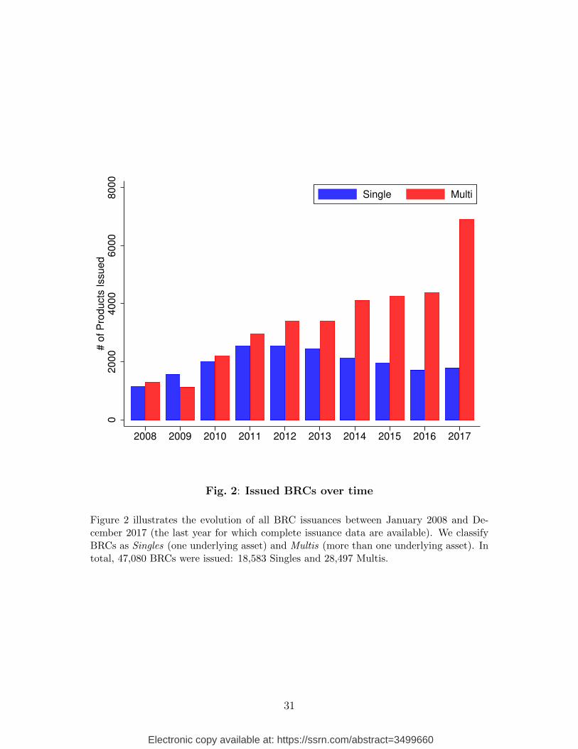
Next, based on this classification, Figure 2 shows the issuance frequencies of Singles and

Multis in Switzerland over time.


Two trends are immediately noticeable from Figure 2. First, the number of BRCs issued

between 2008 and 2017 increases sharply. For instance, while a total of 2,426 BRCs (Singles

and Multis) were issued in 2008, this number almost quadrupled to 8,684 in 2017. Second,

we document a clear shift from less to more complex products over time. More precisely,

while the ratio of issued Multis to Singles was 1.12 in 2008, this number increased to more

than 3.90 in 2017.

2.2. Hypotheses

Given the distinct empirical trends outlined above, we investigate two main questions.

First, we ask what is the difference between Singles and Multis that could explain their

deviating growth rates? To answer this question, we examine both potential supply and

demand-side effects. In line with the results in Celerier and Vallee (2017), we expect that

the issuer margin of a BRC is an increasing function of the product’s complexity. Hence, we

anticipate higher margins for Multis relative to Singles. Accordingly, we state the following

first hypothesis concerning the supply side of BRCs:

7


Hypothesis 1a: Issuers of BRCs earn higher margins from issuing Multis relative to

Singles.

Regarding the demand for BRCs, we expect that investors underestimate the correlation

risk that is contained in Multis but not in Singles. Therefore, retail investors overprice Multis

relative to Singles as they experience difficulties in adjusting for the former’s higher downside

risk. Accordingly, we state the following hypothesis concerning the demand side of BRCs:

Hypothesis 1b: Retail investors systematically underestimate the higher risk of Multis

relative to Singles.

Second, we ask what drives the overall increase in BRCs issued over our sample period?

We expect, in line with Bordalo, Gennaioli, and Shleifer (2015), that investors’ demand for

BRCs increases in times of low interest rates. Accordingly, we state the following hypothesis:

Hypothesis 2: In the search for yield, investors’ willingness to invest in BRCs increases

when risk-free interest rates decrease.

Of course, as in any competitive market, supply and demand for BRCs are determined

endogenously. Hence, to disentangle the two sides as good as possible, we compare our

empirical analysis of BRC field data with a laboratory experiment that aims at isolating

potential demand effects.

3. Data and Methodology

In our empirical analysis, we use data from a commercial platform that provides infor-

mation on all structured products either sold by Swiss issuers or issued in Switzerland.7 The

dataset contains 484,235 structured products of which 53,791 are Barrier Reverse Convert-

ibles. Due to the limited availability of input data for the pricing model, our final sample

7We thank Derivative Partners for providing us with the data.

8


includes in total 4,460 BRCs on US equities issued between January 2008 and December

2017.8 Table 13 in the Appendix lists the top 10 issuers of BRCs in our final sample and the

frequency of product issuances over time.

Several data challenges complicate the creation of our final sample. To obtain all input

data for the pricing model, we rely on various databases. In addition to our initial dataset,

which provides product information regarding the issuer, issue date, expiry date, coupon

rate, barrier level, conversion rate, and the underlying assets, we obtain valuation inputs

from the Center for Research in Security Prices (CRSP), the Option Metrics’ IvyDB US

database, and Bloomberg. To merge the data from different sources, we use the name of the

underlying asset(s) and then their CUSIP number(s) as identifiers. For all underlying assets

in the BRC dataset, we find the closest name in OptionMetrics in terms of the Levenshtein

distance. We validate these pairs and manually allocate name pairs that do not match

perfectly.

3.1. Descriptive Statistics

We present an overview of our final sample in Table 1. Panel A reports product charac-

teristics. The average BRC in our sample offers an annual coupon of 9.29%. The average

maturity is slightly less than one year and the average barrier level is around 67%. In the

following, we describe the input data for our pricing model. To estimate the dividend yield of

the underlying securities, we use data from CRSP. We assume that dividend yields remain

constant over a product’s lifetime and calculate the annual yield as the sum of dividend

payments over the last 12 months prior to issuance divided by the closing price at issuance.

The implied volatilities of the underlying securities are extracted from traded put options.9

First, we search for the closest four options for each underlying asset: the put option with the

8For the representativeness of our final sample, see Table 12 in the Appendix for summary statistics ofall BRCs in the initial dataset.

9As empirical research has shown, the put-call parity does not hold in practice (see e.g., Figlewski andWebb (1993), Amin, Coval, and Seyhun (2004), and Ofek, Richardson, and Whitelaw (2004)). Hence, werestrict ourselves from using call options to infer implied volatilities.

9


closest lower (higher) strike price and closest shorter (longer) maturity before the product’s

expiry date. Second, we bilinearly interpolate the implied volatilities from the corresponding

four options in the two-dimensional space of strike prices and maturities. If one or more of

these four options are not available, we follow the approach of Henderson and Pearson (2011)

and extract the implied volatility from the put option with the nearest expiry date and the

closest strike price. Finally, to obtain the risk-free interest rate, we use the overnight index

swap (OIS) rate with matching maturities based on linear interpolation.

[Insert Table 1 about here]

Panel B of Table 1 provides the average values of the input variables across all underlying

assets in our final sample. The average dividend yield is 2.45%, the average implied volatility

is 33.42%. The latter is relatively high compared to generally observed volatility levels in US

and European stock markets. The average risk-free rate over our sample period is 0.51%.

3.1.1. Measuring Correlations between Underlying Assets

To evaluate Multis, we additionally have to estimate the correlations of their underlying

assets. Since there are no direct market observations of expected correlations, we are partic-

ularly careful in estimating this input variable. Note that the correlation of the underlying

assets crucially affects the fair value of a Multi. The lower the correlation between two as-

sets, the higher the probability of a barrier event. Moreover, lower correlations reduce the

value of Multis as their payoff depends on the worst performing asset. Hence, to account

for possible measurement errors when estimating correlations solely based on the historical

daily log returns, we additionally follow two approaches proposed in the literature: on the

one hand, the shrinkage estimator of Ledoit and Wolf (2004) and, on the other hand, the

shrinkage method of Chen, Wiesel, Eldar, and Hero (2010). Results of all three estimations

are reported in Panel C of Table 1.

10


3.2. Singles vs. Multis

Before examining the relation between product types and issuer margins, we separately

investigate the product characteristics of Singles and Multis, respectively. As described in

Section 2, Singles are BRCs with only one underlying asset, while Multis are BRCs with

more than one underlying asset. Hence, by design, Multis carry a higher risk than Singles

due to their embedded correlation risk. Accordingly, we expect Singles and Multis to differ in

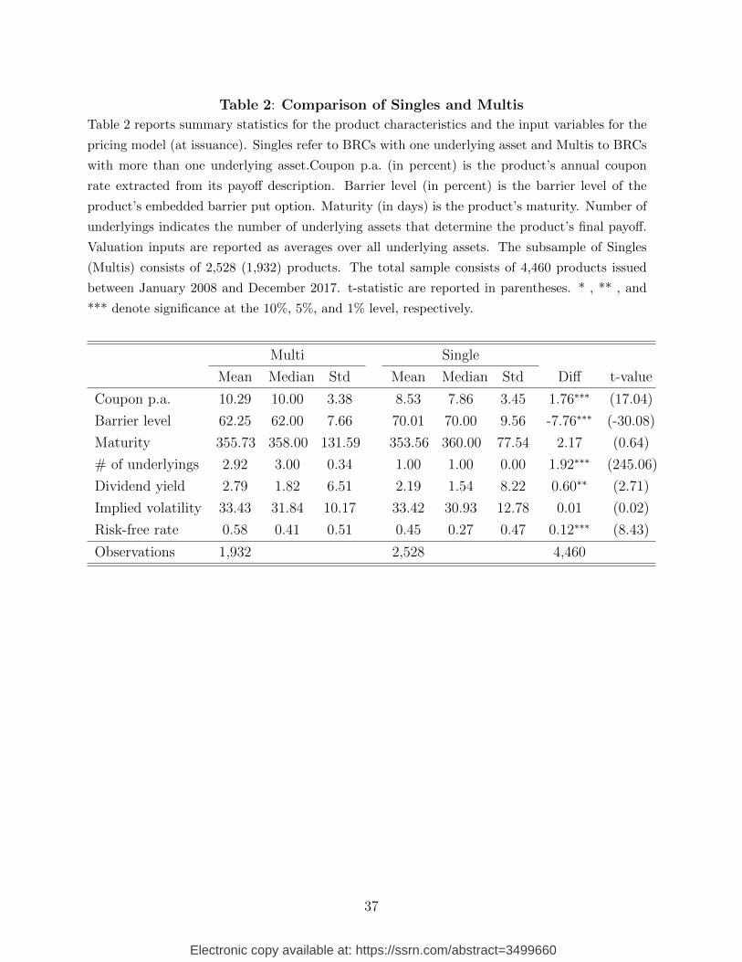
their product characteristics to account for the latter’s higher downside risk. The summary

statistics of the respective characteristics are reported in Table 2.


Our subsamples consist of 2,528 Singles and 1,932 Multis. Note, compared to the total

number of products in our dataset, we lose significantly more observations for Multis than

for Singles. This effect is due to the limited availability of input data for products with more

than one underlying asset. In our sample, Multis are on average based on 2.92 underlying

securities. The average maturity of both product types is slightly shorter than one year.

Multis offer, on average, a 1.76 percentage points higher annual coupon, while their barrier

level is 7.76 percentage points lower. Both differences are statistically significant at the 1%

level. Thus, in both dimensions, Multis’ characteristics are apparently ex-ante more attrac-

tive than those of Singles.10 Notably, however, both product types are based on underlying

assets with similarly high implied volatility levels (around 33% per annum) as well as similar

levels of dividend yields. In total, our final sample covers 546 underlying securities. Table

15 in the Appendix provides an overview of the 30 and 22 most frequently used securities

for Singles and Multis, respectively.

Figure 3 plots the trends of product characteristics and product input variables over time

for both product types. Panel A and C show that the differences between headline rates

and barrier levels remain constant over time. Panel B and Panel D show that there are no

10Multis are issued under a slightly higher risk-free rate than Singles. However, this difference can beexplained by the diverse issuance rates over time.

11


systematic differences in maturity lengths and volatility levels. Interestingly, we observe that

the average annual coupon decreases for both product types. This finding can be reconciled

with the decreasing trend in interest rates over our sample period.


3.3. Pricing Model

Next, we estimate the fair price for each structured product in our sample. The starting

point of our pricing exercise is the closed form solution for BRCs’ embedded down-and-in

put option, under the assumptions of Black and Scholes (1973) (see the pricing formula in

the Appendix). In this model, Singles can be priced in closed form, however, to the best of

our knowledge, Multis cannot. Hence, to derive an accurate pricing model, we proceed as

follows: first, we price Singles according to the closed form model. Second, we again compute

the prices of Singles but this time using a Monte Carlo procedure. We verify the accuracy of

this method by comparing the respective prices.11 Third, after ensuring that our numerical

method leads to similar valuations, we apply the numerical approach to obtain fair values

for all Multis in our sample.

It is well known that the assumptions of constant volatility and no jumps in Black and

Scholes (1973) do not hold in reality. It should be noted, however, that both features generate

leptokurtic returns of the underlying asset(s). Hence, given BRCs asymmetric payoff profile,

both stochastic volatility and jumps increase the probability of a barrier event and lower

values of the underlying asset(s) at maturity. Accordingly, under these assumptions, the fair

values of Singles and Multis would decrease and their margins at issuance would increase.

Thus, we consider our method to yield lower bounds of the actual margins.

11See Table 14 in the Appendix to compare the results of both pricing approaches. The results of theMonte Carlo procedure are based on 365 time steps within a year and 50,000 simulations per product.

12


4. Empirical Results

In this section, we present our empirical results. First, we report estimated BRC margins

at issuance and discuss their determinants for Singles and Multis, respectively. Then we cal-

culate the ex-post performance of both product types. Finally, we highlight the significance

of correlation risk for the margins of Multis.

4.1. Margins at Issuance

To find the margins at issuance, we calculate the fair value of each product according to

the pricing procedure described in Section 3.3. To obtain accurate results, we compute the

margins for Multis based on each of the introduced correlation estimation approaches above.

Using these input data, we calculate the issuer margin for each product as follows:

IMpt =IPpt − FPpt

IPpt

, (1)

where IMpt is the issuer margin at time t for product p. Similarly, IPpt denotes the corre-

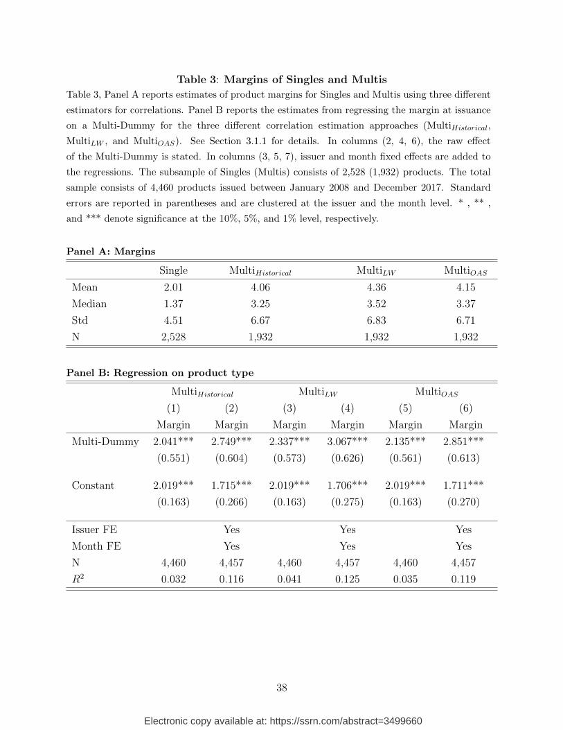
sponding issue price and FPpt its fair price obtained from our pricing model. Table 3, Panel

A, reports the results. We find that the average margin at issuance is 2% for Singles, and

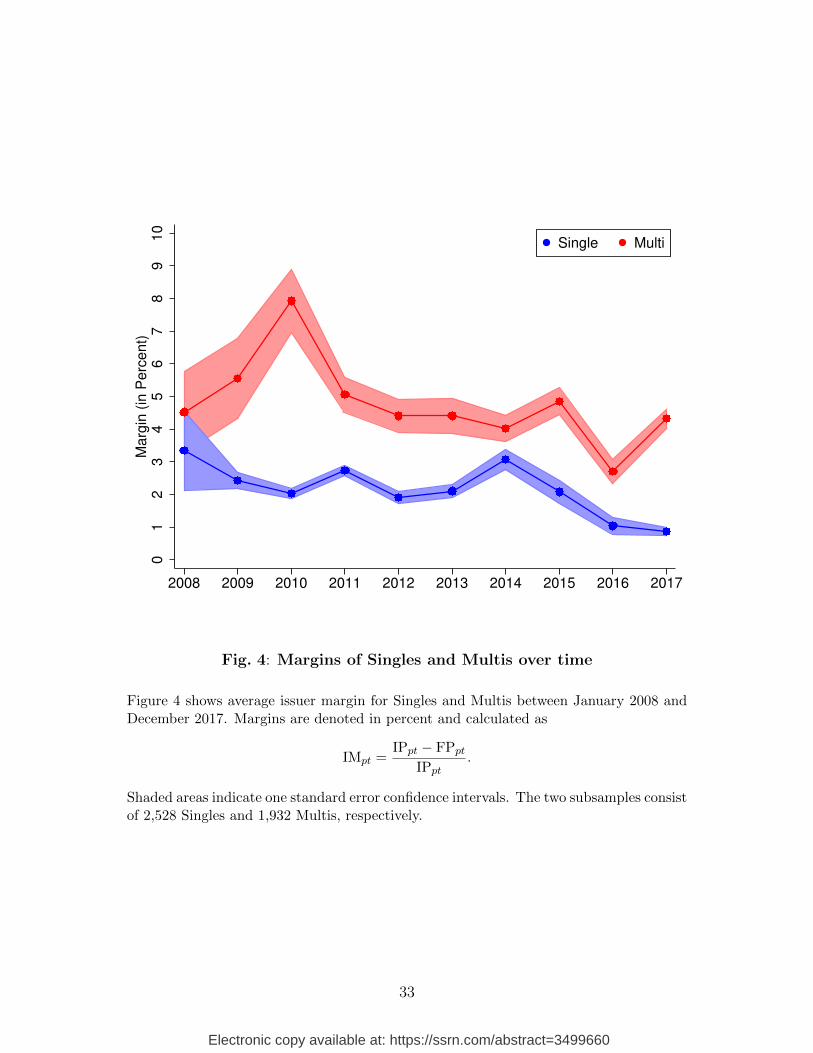
slightly above 4% for Multis. Moreover, Figure 4 shows the average margins of Singles and

Multis over our sample period. These margins are slightly lower than the YEP margins

documented for the US market (see Henderson and Pearson, 2011, Vokata, 2018, and Egan,

2019). Also note that issuers of structured products in Switzerland usually do not charge

any explicit fees.


To analyze the discrepancy in margins between Singles and Multis in more detail, we run

several regressions. In Panel B of Table 3, we regress margins on a Multi-Dummy (equal

to one for Multis). Such a regression allows us to control for fixed effects and to cluster

13


standard errors at the issuer and the month level. Hence, we estimate the following model:

IMjtp = β0 + β1Multi-Dummyp + γFEIssuer + δFEMonth + εpt, (2)

where β1 is the main coefficient of interest, FEIssuer is the issuer fixed effect and FEMonth

the month fixed effect, respectively. Results in Panel B show significantly higher margins

for Multis than for Singles across all specifications. Moreover, when controlling for issuer

and month fixed effects (columns 2, 4, and 6), the difference in margins between the two

product types increases to approximately 2.8 percentage points. Since the margins of Multis

derived from the three different correlation estimations do not vary substantially, we use

in the following, for the sake of simplicity, only the most conservative margins based on

correlations of historical log returns.12


4.2. Margin Drivers for Singles and Multis

Next, to better understand the discrepancy in margins between Singles and Multis, we

explore the relation between product type margins and product characteristics in more detail.

As shown in Section 3.2, certain product characteristics, i.e., the annual coupon and the

barrier level, favor Multis over Singles from an investor perspective. Accordingly, those

product characteristics cannot explain the discrepancy in margins. Thus, this finding must

derive from the product design itself, i.e., the correlation risk that is embedded in Multis but

not in Singles. Therefore, to investigate how the correlation of underlying assets and product

margins are related, we regress the margins of Multis with three underlying assets on product

characteristics and estimated correlations. We fix the number of underlying assets at three

since this represents the “median Multi” (see Table 2). The results of these regressions are

presented in Table 4.

12All results also hold for margins obtained from the other estimation approaches.

14



Table 4 reports a significant decreasing relation between the product margin and the

average correlation (across the underlying assets) and the minimum correlation, respectively.

Intuitively, a lower correlation among the underlying assets, ceteris paribus, results in higher

margins since the probability of a barrier event increases. Moreover, in the case of a barrier

event, the issuer’s payoff is based on the development of the worst performing asset.13 Thus,

the results in Table 4 imply that the lower the correlation between the underlying assets

of a Multi, the higher the margin for its issuer. In other words, lower correlations are not

sufficiently compensated for via high enough coupon (headline) rates.

4.3. Ex-post Performance

So far, we have analyzed BRC margins from the issuers’ perspective. In this subsection,

we report results on the ex-post performance of Singles and Multis from the investors’ point

of view. To get conservative estimates of ex-post performance, we calculate product returns

via realized payoffs and adjust for the risk-free rate at issuance. Hence, the annualized log

return Retpt for product p issued at t is given by:

Retpt =1

(T − t)

[ln

(PayoffpT

IPpt

)− rft(T − t)

], (3)

where PayoffpT is the actual payoff of product p at maturity T , rft the continuous risk-free

rate at issuance, and IPpt the invested amount at issuance. Results are presented in Table

5.


Panel A in Table 5 reports summary statistics of ex-post performances for Singles and

13Hence, a low correlation also increases investors’ risk of receiving lower payoffs. The average correlationis measured as the mean of the three correlations of a product’s underlying assets. The minimum correlationis the lowest correlation.

15


Multis, respectively. Singles on average pay a yearly risk premium of 0.78%. Moreover, in

our sample, the results display considerable variation in returns over time. We find a similar

pattern for Multis. However, Multis on average pay a negative yearly return controlling for

the risk-free rate of −1.62%. During the crisis, investors of Multis on average lost more than

25% of their initial investment relative to the risk-free rate.

Panel B in Table 5 again shows results from product type regressions, this time with

realized returns as the dependent variable:

Retpt = β0 + β1Multi-Dummyp + γFEIssuer + δFEMonth + εpt. (4)

In line with regression (2) in Section 4.1, we find different ex-post returns for Singles and

Multis, while controlling for issuer and month fixed effects. The coefficient of the Multi-

Dummy indicates that Multis on average pay 2.5 percentage points lower returns than Singles

(significant at the 5% level).

4.4. Underlying Assets and Correlation Risk

We have shown that issuers of BRCs charge higher implicit margins for Multis than for

Singles and that realized returns of the former are also lower. This discrepancy in margins,

however, cannot be explained by the primary product characteristics (see Table 2). Hence,

the higher margins for Multis must originate from the difference in the payoff structure

between the two product types, i.e., Multis’ embedded correlation risk. Finally, to investigate

the variation in correlation risk, we take a closer look at the universe of underlying assets in

our sample.

Table 15 in the Appendix reports the 30 most frequent underlying assets of Singles and

Multis. Notably, stocks of big, well-known companies are often used as underlying assets.

However, we do not detect any systematic difference in the selection of underlying assets

between Singles and Multis. Next, we analyze the correlation pattern within our sample. To

16


illustrate the prevalence of correlation risk, we compare the correlation matrix of all stocks in

the S&P 500 (end of 2017)—as a proxy for the universe of possible underlying assets—with

the correlation matrix of the underlying assets in our sample.

[Insert Figure 5 about here]

Figure 5 shows the correlation distributions based on log returns between 2008 and 2017

for S&P 500 member stocks and for the 172 underlying assets used in our final sample,

respectively. We observe a systematic difference between the average correlations among

S&P 500 stocks and among the underlying assets of BRCs (p-value < 0.01). The assets in

our sample correlate considerably less with each other than S&P 500 stocks. Hence, when

issuing Multis, banks seem to systematically combine assets with lower correlations that

increase the correlation risk borne by investors.

5. Experiment

In this second part of our analysis, we present the results from a laboratory experiment

that was designed to carve out and isolate the drivers behind the demand for more complex

BRCs. In particular, it helps us to better understand why Multis—despite their inferior

risk-return profile—are in increasingly higher demand than Singles, as suggested by Figure

2. Moreover, the experiment allows for a controlled investigation of demand sensitivities

with respect to different market environments, i.e., varying volatility and interest rate levels.

The chosen design aims to elicit individuals’ subjective valuation of Singles and Multis and

their willingness to invest in BRCs in general.

5.1. Design

Here we present the general setup of the experiment together with the actual task that

subjects had to perform. The experiment was fully computerized using z-Tree (Fischbacher,

17


2007).

For the experiment, we created two synthetic product types mimicking the payoff pro-

files of actual BRCs. In particular, subjects were presented with synthetic “Singles” whose

payoff depended on the evolution of one underlying asset and synthetic “Multis” whose pay-

off depended on the evolution of the worse performing asset out of two underlying assets,

respectively.14 To examine our different hypotheses, we use a 2× 3 ( 2 volatility treatments

and 3 risk-free rate levels) design to control for the effects of different investment environ-

ments (see Table 6).15 In each of the six treatments (rounds), subjects were given the chance

to either buy a Single or a Multi (see Table 7) or, alternatively, invest their money at the

risk-free interest rate. Importantly, our design allows for both a between and within-subject

analysis.16 The latter requires each subject to be exposed to all treatments, which in turn

enables us to control for the idiosyncratic attributes of each subject’s behavior.

At the beginning of each round, subjects were endowed with a fixed amount of ini-

tial wealth (130 Experimental Currency Units (ECU)), which they could freely invest.17

Moreover, all subjects received information about the available products and the general

investment environment, i.e., the prevailing risk-free rate and volatility level. To limit the

complexity of the task, the Multi’s underlying asset prices always evolved independently

of each other (ρ = 0). To further facilitate subjects’ evaluation of the available products,

the software calculated expected final payoffs based on subjects’ estimates of (i) the prob-

ability of a barrier event and (ii) the expected value of the payoff-relevant underlying asset

14Designing new synthetic products instead of using real BRCs has two advantages. First, it allows us tocontrol each parameter separately and therefore greatly simplifies effect identification. Second, we avoid theproblem that subjects have different levels of (self-perceived) expertise about real stock markets and starttrying to identify historical price patterns.

15In a second part of the experiment, we also introduced a treatment with risk-adjusted coupons. Morespecifically, the coupons were chosen such that both Singles and Multis had identical fair values assumingrisk neutrality. While the general underestimation of the Multis’ correlation risk (see below) prevails, thereis no significant difference between the willingness-to-pay for Singles vs. Multis. This result is in line with ahigher subjective discount applied to Multis relative to Singles.

16In a between-subjects design, the various experimental treatments are given to different participants,while in a within-subjects design, all participants perform all various treatments.

17In a subsample, subjects were endowed with 140 ECU instead. There are no significant effects associatedwith this slight increase in initial endowments.

18


conditional on (i).

At the first stage of each round, subjects had to indicate their willingness-to-pay (WTP)

for both product types—Single and Multi—separately. Importantly, to elicit individuals’

unbiased WTP, we employed the incentive-compatible mechanism proposed by Becker, De-

Groot, and Marschak (1964). Specifically, for an extensive list of possible prices,18 subjects

had to indicate whether or not they were willing to buy each product at each given price.

The actual price for each product was then randomly drawn from this predetermined price

list (with uniform probabilities). Whenever the randomly drawn price was lower or equal

to subjects’ WTP, they were allocated the product in return for the random price and any

remaining wealth was invested at the risk-free rate. In contrast, whenever the randomly

drawn price was higher than subjects’ WTP, their entire wealth was invested at the risk-free

rate by default. To ensure that subjects evaluated both product types independently, the

above procedure was only executed for one randomly chosen product in each round. Finally,

subjects always had the option to opt out of investing in BRCs altogether and, independent

of the randomly drawn price, invest all their wealth at the prevailing risk-free rate.

At the second stage of each round, after each subject’s investment decision had been

implemented, actual payoffs were determined and subjects’ final wealth was calculated. In

addition, the realized price paths of the products’ underlying assets were displayed and the

corresponding scenario (occurrence vs. absence of barrier event) indicated. All rounds were

entirely independent of each other, i.e., at the beginning of every round, subjects’ initial

wealth was reset.

5.1.1. Procedural Details

The experiment was conducted in March and October 2018 at the computer laboratory of

the Department of Banking and Finance at the University of Zurich. We ran the experiment

18The price list ranged from a minimum price of ECU 60 to the highest achievable payoff of ECU 117.

19


with seven different cohorts, resulting in a sample of 125 students.19 Table 8 provides the

summary statistics across all participating individuals. Subjects are on average 23 years

old, a slightly more than half are female, and around one third consider themselves familiar

with structured products (self-reported). Following Isaac, Walker, and Williams (1994),

Selten, Mitzkewitz, and Uhlich (1997), Biais, Hilton, Mazurier, and Pouget (2005), and

Williams (2008), subjects’ final wealth from one randomly selected round was converted into

points that counted towards their final grade. The written instructions contained various

comprehension questions that controlled for subjects’ understanding of the task. Subjects

were only allowed to proceed to the practice round after they had answered those questions

correctly. If necessary, further explanations were provided by the experimenter. To avoid

order effects, a computerized randomization function was used to determine the sequence of

rounds. On average, one session lasted about 90 minutes.

5.2. Experimental Results

We first describe the results at an aggregate level before turning to a more detailed

discussion of the different treatment effects and the influence of subjects’ personal traits on

product margins.

5.2.1. Implied Margins

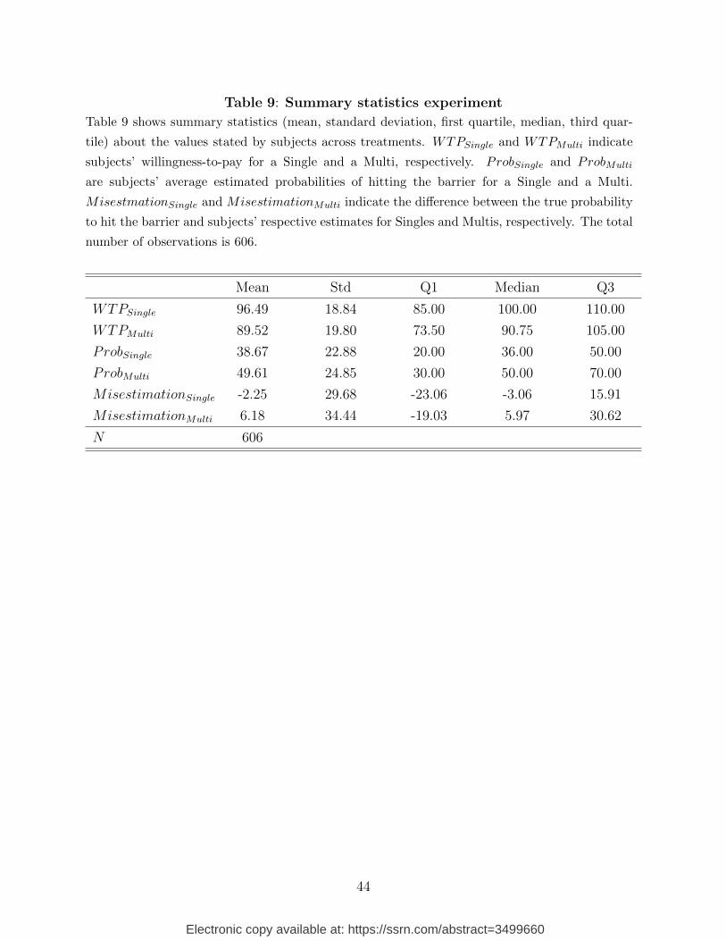
Table 9 presents the summary statistics on the main experimental variables across treat-

ments. We find that subjects value Singles and Multis differently. On average, they are

willing to pay ECU 96.49 for a Single and ECU 89.52 for a Multi. Hence, subjects seem to

partially adjust for the latter’s higher risk of a barrier event. Table 9 also shows subjects’

average probability estimates of a barrier event for both Singles and Multis, respectively.

We measure the quality of their risk assessment by looking at the difference between the

19Subjects had at least some basic knowledge of finance. Therefore, we consider it plausible that actualretail investors are relatively even more likely to misestimate Multis’ embedded correlation risk.

20


true probabilities and subjects’ respective estimates. On average, subjects slightly overes-

timate Singles’ inherent risk of a barrier event, while they substantially underestimate the

corresponding risk for Multis (see below).


Since the risk-neutral fair price for each product depends on the prevailing investment

environment, we cannot directly compare revealed WTP levels across rounds. In line with

Section 4, we therefore calculate each subject i’s implicit margin for product p as

IMip =WTPip − FPp

WTPip

, (5)

where FPp denotes product p’s fair value under risk neutrality. Hence, a product’s implicit

margin is defined as the percentage difference between subjects product-specific WTP and

its fair price assuming risk-neutral preferences. This approach allows for a conservative

comparison between Singles and Multis across the different treatments.

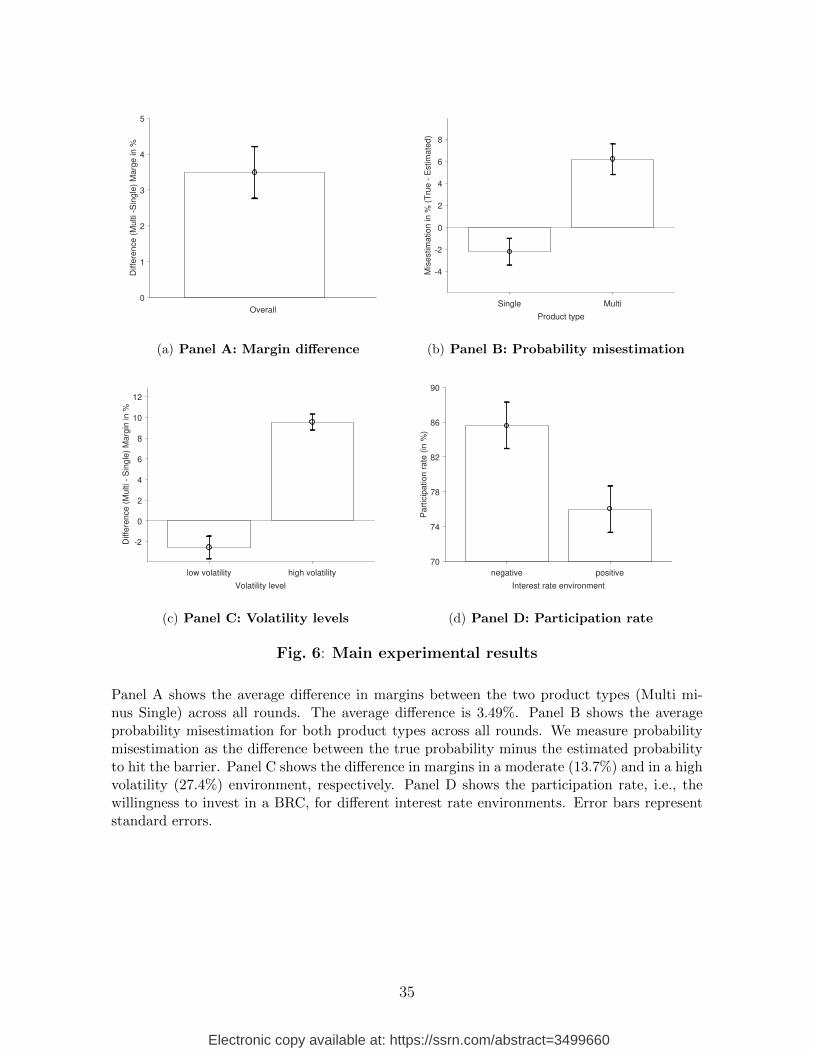
Our results demonstrate that subjects overvalue Multis relative to Singles. Panel A in

Figure 6 shows the average difference in margins between the two product types. Overall,

the implicit margin for Multis is 3.49% higher than for Singles. A two-sided t-test strongly

rejects the null hypothesis of identical margins (p-value < 0.01).

To control for confounding effects, we regress product margins on a Multi-Dummy (equal

to one for Multis) while controlling for subjects’ investment decision, the volatility level, and

the risk-free interest rate. Table 10 shows the results of different regression specifications.

In the first model, we include subject fixed effects, whereas in the second model we control

for subject characteristics such as gender, age, risk preferences, and overconfidence. For

both specifications, we find that Multis generate significantly higher margins for the issuer

(p-value < 0.01). Regarding individual subject characteristics, we document that margins

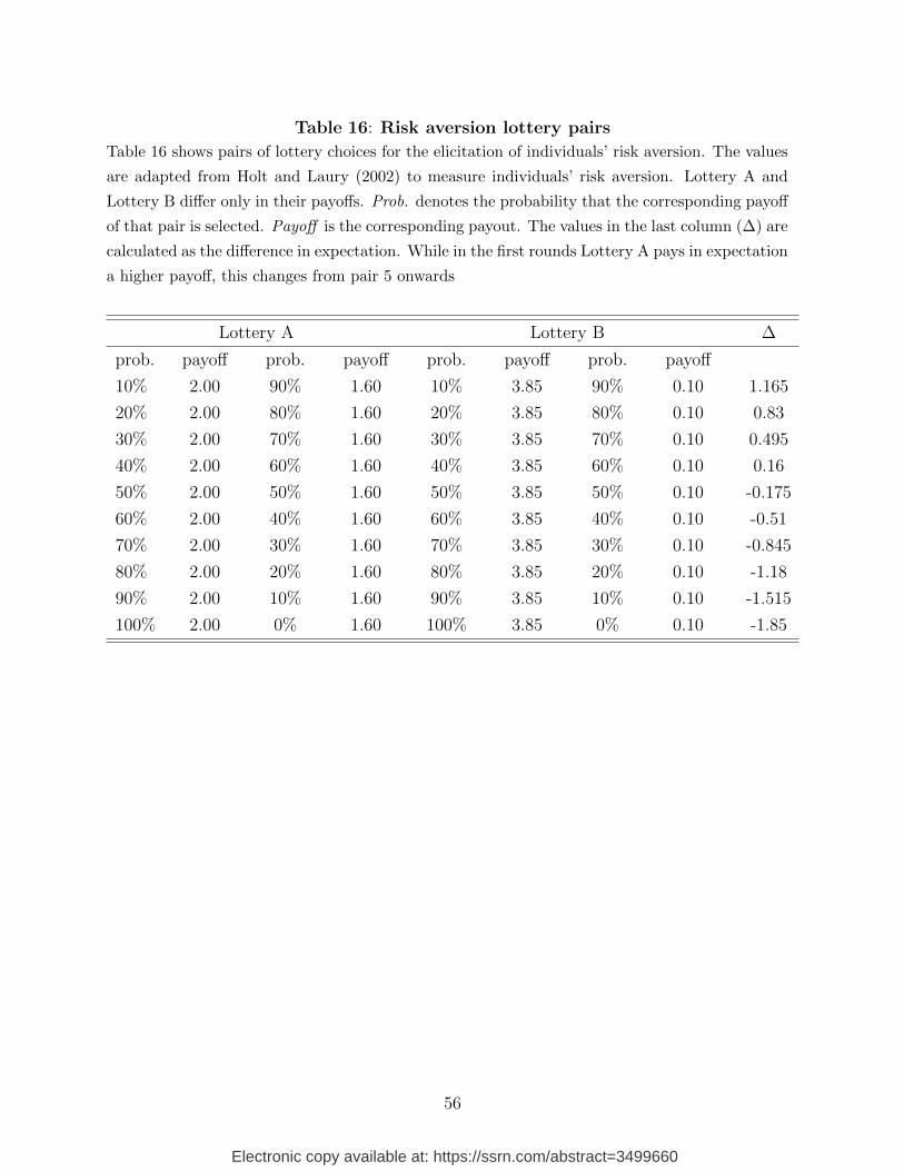
are decreasing in subjects’ risk aversion and increasing in their level of overconfidence. Risk

preferences are measured as in Holt and Laury (2002), while overconfidence is assessed

21


according to the interval production task proposed by Alpert and Raiffa (1982). Figure

9 and Figure 10 in the Appendix provide scatter plots with the corresponding best linear

fits. Interestingly, Figure 10 suggests that subjects’ degree of judgmental overconfidence

substantially drives the margins of Multis but does not significantly affect the margins of

Singles.


Drawing an interim conclusion, our experiment complements the findings in Section 4 in

showing that BRC investors are more likely to buy overpriced Multis than Singles. In the

following, we analyze the mechanism behind this demand-side effect in more detail.

5.2.2. Volatility Levels and Probability Misestimation

In each round, both product types exhibit identical characteristics except that the final

payoff of a Single is based on one underlying asset, while the corresponding payoff of a

Multi depends on the performance of one additional underlying assets. As noted above,

the respective underlying asset prices of the two assets evolve independently. Hence, by

design, Multis always have a higher probability of a barrier event than Singles. Moreover,

Multis’ worst-off payoff characteristic further amplifies the risk of low payoffs at maturity.

The unconditional difference in average margins between Singles and Multis shown in Panel

A in Figure 6 indicates that subjects generally fail to fully adjust for this different extent of

downside risk.

We find a systematic bias in subjects’ estimates of Multis’ downside risk. Panel B in Fig-

ure 6 shows that subjects are relatively accurate in assessing the probability of a barrier event

for Singles. However, they significantly underestimate the corresponding risk for Multis. On

average, subjects slightly overestimate Singles’ probability of a barrier event by 2.25%, while,

in the case of Multis, they significantly underestimate it by 6.18%. Importantly, the only

explanation for this relative difference lies in the inability to correctly account for Multis’

22


inherent correlation risk. They sufficiently adjust their subjective evaluations for the risk

induced by one single underlying asset but fail to do so in the presence of two underlying

assets.

To investigate this finding in more detail, we examine the correlation between subjects’

probability misestimation and the corresponding margins. As expected, product margins

strongly correlate with subjects’ misestimation. In other words, when subjects accurately

estimate the probability of a barrier event, margins are close to zero, while in the case

of imprecise probability estimates, margins are significantly different from zero (Pearson-

correlation coefficient equal to 0.63, p-value < 0.01).

In line with this result, we find that an increase in the volatility of the underlying asset(s)

increases the discrepancy in margins between product types. A rise in volatility also increases

the likelihood of a barrier event and low(er) payoff scenarios. Hence, ceteris paribus, the

value of BRCs decreases. Subjects estimate both the probability of a barrier event and the

conditional payoffs fairly accurately under moderate volatility levels (13.7% per unit of time),

whereas they experience more difficulties doing so in a high volatility environment (27.4%).

Panel C in Figure 6 documents this finding. A two-sided t-test rejects the hypothesis of no

difference in margins between Singles and Multis in the high volatility environment (p-value

< 0.01).

5.2.3. Interest Rate Environment

Relying on the power of laboratory control, we isolate the impact of different interest rate

levels on subjects’ demand for BRCs. Bordalo et al. (2015) show that, in a low interest rate

environment, it can prove profitable for issuers to cater to yield-seeking investors. To test

this idea in our setting, we introduce different spreads between the yield of BRCs and the

prevailing risk-free interest rate (see Table 6). Between these treatments, we are particularly

interested in differences in subjects’ participation rate, i.e., in the proportion of subjects

willing to invest in either Singles or Multis as opposed to the risk-free alternative. For each

23


subject, the participation rate equals the proportion of rounds for which she did not decide

to opt out of the implicit bidding process. Panel D in Figure 6 shows average participation

rates for the negative and non-negative interest rate environments, respectively. A Wilcoxon

signed rank test rejects the null hypothesis of identical participation rates (p-value < 0.01).

The difference between negative and zero interest rates turns out to be insignificant.


Table 11 documents the results from corresponding logistic regressions. The estimated

coefficients imply that, under positive interest rates (3% per time unit), the proportion of

subjects willing to invest in BRCs declines on average by 10% relative to zero and negative

(-2%) interest rates.

6. Conclusion

Celerier and Vallee (2017) show that the complexity of retail structured products has

increased substantially since the financial crisis. Zingales (2015) argues that such an increase

may not be for the benefit of society at large. In this paper, we provide further evidence for

this hypothesis.

Analyzing 4,460 yield enhancement products issued in Switzerland between 2008 and

2017, we deliberately focus on the main product feature influencing complexity, i.e., the

number of underlying assets. Starting from total issuance numbers, we document a substan-

tial shift from less to more complex products over time. We find that banks’ ex-ante margins

are increasing while investors’ realized returns are decreasing in product complexity. Our

empirical analysis suggests uncompensated correlation risk as the driving mechanism behind

both phenomena.

By conducting a laboratory experiment, we then confirm that subjects indeed fail to fully

account for the inherent correlation risk of products with multiple underlying assets. In line

with Bordalo et al. (2015), we also find that subjects are more likely to invest in structured

24


products whenever the less risky outside option provides lower returns. Intuitively, subjects

prone to judgmental overconfidence overvalue more complex products more severely.

Overall, our findings emphasize the importance of regulators’ vigilance in overseeing

the suppliers of retail structured products. During the current times of unprecedented low

interest rates, educating yield-seeking households about the complete risk-return profile of

available investment opportunities becomes particularly important. In the specific case of

reverse convertibles on multiple underlying assets, such educational efforts should foster the

understanding of the embedded correlation risk shrouded by the promise of high coupon

payments.

25


References

Allen, F., Gale, D., 1994. Financial innovation and risk sharing. MIT press.

Alpert, M., Raiffa, H., 1982. A progress report on the training of probability assessors. In:

Kahneman, D., Slovic, P., Tversky, A. (eds.), Judgment Under Uncertainty: Heuristics

and Biases , Cambridge University Press, pp. 294–305.

Amin, K., Coval, J. D., Seyhun, H. N., 2004. Index option prices and stock market momen-

tum. The Journal of Business 77, 835–874.

Ammann, M., Arnold, M., Straumann, S., 2018. Illuminating the dark side of financial

innovation: The role of investor information. Working Paper .

Becker, G. M., DeGroot, M. H., Marschak, J., 1964. Measuring utility by a single-response

sequential method. Systems Research and Behavioral Science 9, 226–232.

Biais, B., Hilton, D., Mazurier, K., Pouget, S., 2005. Judgemental overconfidence, self-

monitoring, and trading performance in an experimental financial market. The Review of

Economic Studies 72, 287–312.

Black, F., Scholes, M., 1973. The pricing of options and corporate liabilities. Journal of

Political Economy 81, 637–654.

Bordalo, P., Gennaioli, N., Shleifer, A., 2015. Competition for attention. The Review of

Economic Studies pp. 481–513.

Carlin, B. I., 2009. Strategic price complexity in retail financial markets. Journal of financial

Economics 91, 278–287.

Carlin, B. I., Kogan, S., Lowery, R., 2013. Trading complex assets. The Journal of Finance

68, 1937–1960.

26


Carlin, B. I., Manso, G., 2011. Obfuscation, learning, and the evolution of investor sophisti-

cation. Review of Financial Studies 24, 754–785.

Celerier, C., Vallee, B., 2017. Catering to investors through security design: Headline rate

and complexity. The Quarterly Journal of Economics 132, 1469–1508.

Chen, Y., Wiesel, A., Eldar, Y. C., Hero, A. O., 2010. Shrinkage algorithms for mmse

covariance estimation. IEEE Transactions on Signal Processing 58, 5016–5029.

Chesney, M., 2018. A Permanent Crisis: The Financial Oligarchy’s Seizing of Power and the

Failure of Democracy. Palgrave Macmillan.

Chesney, M., Krakow, J., Maranghino-Singer, B., Munstermann, L., 2018. Asset Pricing:

Finanzderivate und ihre Systemrisiken. Springer-Verlag.

Duffie, D., Rahi, R., 1995. Financial market innovation and security design: An introduction.

Journal of Economic Theory 65, 1–42.

Egan, M., 2019. Brokers versus retail investors: Conflicting interests and dominated prod-

ucts. The Journal of Finance 74, 1217–1260.

Ellison, G., 2005. A model of add-on pricing. The Quarterly Journal of Economics 120,

585–637.

ESMA, 2018. Trends, risks and vulnerabilities. ESMA Report 2.

FCA, 2015. Structured products: Thematic review of product development and governance.

Figlewski, S., Webb, G. P., 1993. Options, short sales, and market completeness. The Journal

of Finance 48, 761–777.

Fischbacher, U., 2007. z-tree: Zurich toolbox for ready-made economic experiments. Exper-

imental Economics 10, 171–178.

27


Gabaix, X., Laibson, D., 2005. Shrouded attributes, consumer myopia, and information

suppression in competitive markets. Tech. rep., National Bureau of Economic Research.

Ghent, A. C., Torous, W. N., Valkanov, R. I., 2017. Complexity in structured finance. The

Review of Economic Studies 86, 694–722.

Henderson, B. J., Pearson, N. D., 2011. The dark side of financial innovation: A case study

of the pricing of a retail financial product. Journal of Financial Economics 100, 227–247.

Holt, C. A., Laury, S. K., 2002. Risk aversion and incentive effects. American Economic

Review 92, 1644–1655.

Isaac, R. M., Walker, J. M., Williams, A. W., 1994. Group size and the voluntary provision

of public goods: Experimental evidence utilizing large groups. Journal of public Economics

54, 1–36.

Ledoit, O., Wolf, M., 2004. A well-conditioned estimator for large-dimensional covariance

matrices. Journal of Multivariate Analysis 88, 365–411.

Ofek, E., Richardson, M., Whitelaw, R. F., 2004. Limited arbitrage and short sales restric-

tions: Evidence from the options markets. Journal of Financial Economics 74, 305–342.

Rieger, M. O., 2012. Why do investors buy bad financial products? probability misestimation

and preferences in financial investment decision. Journal of Behavioral Finance 13, 108–

118.

SEC, 2011. Staff summary report on issues identified in examinations of certain structured

securities products sold to retail investors. SEC Report .

Selten, R., Mitzkewitz, M., Uhlich, G. R., 1997. Duopoly strategies programmed by experi-

enced players. Econometrica: Journal of the Econometric Society pp. 517–555.

SVSP, 2019. Market report structured products. Schweizer Verband fur Strukturierte Pro-

dukte, Quarterly Report 1.

28


Vokata, P., 2018. Engineering lemons. Working paper .

Wallmeier, M., Diethelm, M., 2009. Market pricing of exotic structured products: The case

of multi-asset barrier reverse convertibles in switzerland. The Journal of Derivatives 17,

59–72.

Williams, A. W., 2008. Price bubbles in large financial asset markets. Handbook of Experi-

mental Economics Results 1, 242–246.

Zingales, L., 2015. Presidential address: Does finance benefit society? The Journal of Finance

70, 1327–1363.

29


Figures and Tables

Fig. 1: Barrier Reverse Convertible

Figure 1 displays the payoff profile of a barrier reverse convertible (BRC) with one un-derlying asset. The horizontal axis denotes the final value of the underlying asset atmaturity. The vertical line measures the payoff based on the final value of the underlyingasset at maturity plus the coupon payment. The dashed line indicates the barrier level.If the price of the underlying asset touches the barrier during the life of the product, thebond principal is converted into holdings of the underlying asset at a predefined ratio.However, the final principal payment paid by the issuer is capped at par (100%).

30


02

00

04

00

06

00

08

00

0#

of

Pro

du

cts

Issu

ed

2008 2009 2010 2011 2012 2013 2014 2015 2016 2017

Single Multi

Fig. 2: Issued BRCs over time

Figure 2 illustrates the evolution of all BRC issuances between January 2008 and De-cember 2017 (the last year for which complete issuance data are available). We classifyBRCs as Singles (one underlying asset) and Multis (more than one underlying asset). Intotal, 47,080 BRCs were issued: 18,583 Singles and 28,497 Multis.

31


04

812

16

20

Coupon p

.a. (in P

erc

ent)

2008 2009 2010 2011 2012 2013 2014 2015 2016 2017

Single Multi

(a) Panel A: Headline rate0

100

200

300

400

500

Matu

rity

(in

Days)

2008 2009 2010 2011 2012 2013 2014 2015 2016 2017

Single Multi

(b) Panel B: Maturity

50

60

70

80

90

100

Barr

ier

Level (in P

erc

ent)

2008 2009 2010 2011 2012 2013 2014 2015 2016 2017

Single Multi

(c) Panel C: Barrier level

05

10

15

20

25

30

35

40

45

50

Vola

tilit

y (

in P

erc

ent)

2008 2009 2010 2011 2012 2013 2014 2015 2016 2017

Single Multi

(d) Panel D: Implied volatility

Fig. 3: Product characteristics of Singles and Multis over time

Figure 3 shows the annual headline rate (coupon p.a.) in percent (Panel A), the maturitymeasured in calendar days (Panel B), the barrier level measured in percent (Panel C), andthe annual volatility in percent (Panel D) for both product types, Single (blue) and Multi(red), between January 2008 and December 2017. Shaded areas indicate one standarderror confidence intervals. The two subsamples consist of 2,528 Singles and 1,932 Multis,respectively.

32


01

23

45

67

89

10

Ma

rgin

(in

Pe

rce

nt)

2008 2009 2010 2011 2012 2013 2014 2015 2016 2017

Single Multi

Fig. 4: Margins of Singles and Multis over time

Figure 4 shows average issuer margin for Singles and Multis between January 2008 andDecember 2017. Margins are denoted in percent and calculated as

IMpt =IPpt − FPpt

IPpt.

Shaded areas indicate one standard error confidence intervals. The two subsamples consistof 2,528 Singles and 1,932 Multis, respectively.

33


−0.6 −0.4 −0.2 0.0 0.2 0.4 0.6 0.8 1.0Correlation

0.0

0.5

1.0

1.5

2.0

2.5

3.0

Density

Mean correlation S&P500Mean correlation sampleS&P500Sample

Fig. 5: Correlation distributions

Figure 5 shows the correlation distributions between 2008 and 2017 for both S&P 500member stocks and the 172 underlying assets in our final sample (whereof 101 are membersof the S&P 500). S&P 500 members are selected according to the index’s constituent listas of the end of 2017. Correlations are based on daily log returns.

34


Overall

0

1

2

3

4

5

Diffe

ren

ce

(M

ulti -S

ing

le)

Ma

rge

in

%

(a) Panel A: Margin difference

Single Multi

Product type

-4

-2

0

2

4

6

8

Mis

estim

atio

n in

% (

Tru

e -

Estim

ate

d)

(b) Panel B: Probability misestimation

low volatility high volatility

Volatility level

-2

0

2

4

6

8

10

12

Diffe

ren

ce

(M

ulti -

Sin

gle

) M

arg

in in

%

(c) Panel C: Volatility levels

negative positive

Interest rate environment

70

74

78

82

86

90

Pa

rtic

ipa

tio

n r

ate

(in

%)

(d) Panel D: Participation rate

Fig. 6: Main experimental results

Panel A shows the average difference in margins between the two product types (Multi mi-nus Single) across all rounds. The average difference is 3.49%. Panel B shows the averageprobability misestimation for both product types across all rounds. We measure probabilitymisestimation as the difference between the true probability minus the estimated probabilityto hit the barrier. Panel C shows the difference in margins in a moderate (13.7%) and in a highvolatility (27.4%) environment, respectively. Panel D shows the participation rate, i.e., thewillingness to invest in a BRC, for different interest rate environments. Error bars representstandard errors.

35


Table 1: Summary statistics full sample

Table 1 reports summary statistics of product characteristics at issuance (Panel A) and inputs

for the pricing model (Panel B). Coupon p.a. (in percent) is the product’s annual coupon rate

extracted from its payoff description. Barrier level (in percent) is the barrier level of the product’s

embedded barrier put option. Maturity (in days) is the product’s maturity. Number of underlyings

indicates the number of underlying assets that determine the product’s final payoff. Valuation

inputs are reported as averages over all underlying assets. The sample consists of 4,460 products

issued between January 2008 and December 2017.

Panel A: Product characteristics

Mean Std Min Q1 Median Q3 Max

Coupon p.a. 9.29 3.53 0.00 6.94 8.65 10.88 57.34

Barrier level 66.65 9.59 39.00 59.00 69.00 75.00 90.00

Maturity 354.50 104.45 60 357 358 386 1,093

Number of underlyings 1.83 0.98 1 1 1 3 4

Observations 4,460

Panel B: Valuation inputs

Dividend yield 2.45 4.53 0.00 0.51 1.71 2.71 18.12

Implied volatility 33.42 11.72 13.53 25.15 31.34 38.97 123.37

Risk-free rate 0.51 0.49 0.06 0.14 0.32 0.60 3.09

Observations 4,460

Panel C: Correlation estimates

Correlationraw 44.89 21.39 -2.14 29.01 44.21 57.45 91.19

CorrelationLW 38.31 24.45 0.00 20.71 38.86 53.14 88.38

CorrelationOAS 43.07 21.56 -1.38 27.12 42.35 55.80 89.48

Observations 1,932

36


Table 2: Comparison of Singles and Multis

Table 2 reports summary statistics for the product characteristics and the input variables for the

pricing model (at issuance). Singles refer to BRCs with one underlying asset and Multis to BRCs

with more than one underlying asset.Coupon p.a. (in percent) is the product’s annual coupon

rate extracted from its payoff description. Barrier level (in percent) is the barrier level of the

product’s embedded barrier put option. Maturity (in days) is the product’s maturity. Number of

underlyings indicates the number of underlying assets that determine the product’s final payoff.

Valuation inputs are reported as averages over all underlying assets. The subsample of Singles

(Multis) consists of 2,528 (1,932) products. The total sample consists of 4,460 products issued

between January 2008 and December 2017. t-statistic are reported in parentheses. * , ** , and

*** denote significance at the 10%, 5%, and 1% level, respectively.

Multi Single

Mean Median Std Mean Median Std Diff t-value

Coupon p.a. 10.29 10.00 3.38 8.53 7.86 3.45 1.76∗∗∗ (17.04)

Barrier level 62.25 62.00 7.66 70.01 70.00 9.56 -7.76∗∗∗ (-30.08)

Maturity 355.73 358.00 131.59 353.56 360.00 77.54 2.17 (0.64)

# of underlyings 2.92 3.00 0.34 1.00 1.00 0.00 1.92∗∗∗ (245.06)

Dividend yield 2.79 1.82 6.51 2.19 1.54 8.22 0.60∗∗ (2.71)

Implied volatility 33.43 31.84 10.17 33.42 30.93 12.78 0.01 (0.02)

Risk-free rate 0.58 0.41 0.51 0.45 0.27 0.47 0.12∗∗∗ (8.43)

Observations 1,932 2,528 4,460

37


Table 3: Margins of Singles and Multis

Table 3, Panel A reports estimates of product margins for Singles and Multis using three different

estimators for correlations. Panel B reports the estimates from regressing the margin at issuance

on a Multi-Dummy for the three different correlation estimation approaches (MultiHistorical,

MultiLW , and MultiOAS). See Section 3.1.1 for details. In columns (2, 4, 6), the raw effect

of the Multi-Dummy is stated. In columns (3, 5, 7), issuer and month fixed effects are added to

the regressions. The subsample of Singles (Multis) consists of 2,528 (1,932) products. The total

sample consists of 4,460 products issued between January 2008 and December 2017. Standard

errors are reported in parentheses and are clustered at the issuer and the month level. * , ** ,

and *** denote significance at the 10%, 5%, and 1% level, respectively.

Panel A: Margins

Single MultiHistorical MultiLW MultiOAS

Mean 2.01 4.06 4.36 4.15

Median 1.37 3.25 3.52 3.37

Std 4.51 6.67 6.83 6.71

N 2,528 1,932 1,932 1,932

Panel B: Regression on product type

MultiHistorical MultiLW MultiOAS

(1) (2) (3) (4) (5) (6)

Margin Margin Margin Margin Margin Margin

Multi-Dummy 2.041*** 2.749*** 2.337*** 3.067*** 2.135*** 2.851***

(0.551) (0.604) (0.573) (0.626) (0.561) (0.613)

Constant 2.019*** 1.715*** 2.019*** 1.706*** 2.019*** 1.711***

(0.163) (0.266) (0.163) (0.275) (0.163) (0.270)

Issuer FE Yes Yes Yes

Month FE Yes Yes Yes

N 4,460 4,457 4,460 4,457 4,460 4,457

R2 0.032 0.116 0.041 0.125 0.035 0.119

38


Table 4: Multis with three underlying assets

Table 4 shows results from regressing the margin at issuance on the correlation of the underlying

assets for Multis with three underlying assets. In columns 2-4, we regress margins on average

correlations of historical log returns of the underlying assets. For each product, the average

correlation is measured as the average across all three correlation pairs. In columns 5-7, we regress

margins on minimum correlations. The minimum correlation is the smallest correlation across

all three correlation pairs. Controls include product characteristics, i.e., coupon p.a., maturity,

barrier level, implied volatility, dividend yield, and risk-free rate (see Table 17 in the Appendix

for details). Standard errors are reported in parentheses and are clustered at the issuer and the

month level. * , ** , and *** denote significance at the 10%, 5%, and 1% level, respectively.

(1) (2) (3) (4) (5) (6)

Margin Margin Margin Margin Margin Margin

Average correlation -0.029∗∗∗ -0.073∗∗∗ -0.077∗∗∗

(0.004) (0.005) (0.005)

Minimum correlation -0.031∗∗∗ -0.076∗∗∗ -0.078∗∗∗

(0.004) (0.005) (0.005)

Controls Yes Yes Yes Yes

Issuer FE Yes Yes

Month FE Yes Yes

N 1,691 1,691 1,679 1,691 1,691 1,679

R2 0.010 0.842 0.864 0.011 0.845 0.866

39


Table 5: Ex-post performance of Singles and Multis

Table 5 reports summary statistics of ex-post performance for Singles and Multis (Panel A) and

results from regressing ex-post performance on a Multi-Dummy (Panel B). The Table reports

average returns by year of issuance. The subsample of Singles (Multis) consists of 2,528 (1,932)

products. The total sample consists of 4,460 products issued between January 2008 and December

2017. Standard errors are reported in parentheses and are clustered at the issuer and the month

level. * , ** , and *** denote significance at the 10%, 5%, and 1% level, respectively.

Panel A: Ex-post product return

Single Multi

Mean N Mean N

2008 -7.80 68 -25.12 27

2009 11.75 114 14.71 38

2010 7.54 142 7.44 101

2011 -2.12 246 2.98 143

2012 0.91 283 -6.64 158

2013 0.64 295 -10.12 147

2014 -5.92 373 -16.22 267

2015 -0.57 335 -2.86 240

2016 6.82 317 6.86 328

2017 1.14 355 2.30 483

Total 0.78 2,528 -1.62 1,932

Panel B: Regression on product type

Product return Product return

Multi-Dummy -2.401* -2.564**

(1.245) (0.932)

Constant 0.781 0.848**

(0.530) (0.387)

Issuer FE Yes

Month FE Yes

N 4,460 4,457

R2 0.004 0.155

40


Table 6: Treatment overviewTable 6 shows an overview of the different experimental treatments. Treatments differ along the

interest rate and the volatility dimension. In each treatment, the respective parameter changes,

e.g., the volatility level (moderate vs. high) of the underlying assets, or the level of the risk-free

interest rate (negative vs. zero vs. positive).

Interest environment

(3.00%) (0.00%) (-2.00%)

Vol

atilit

yle

vel

moderate (13.7%) Treatment 1 Treatment 2 Treatment 3

high (27.4%) Treatment 4 Treatment 5 Treatment 6

41


Table 7: Product parameters overview

Table 7 provides an overview of the products and their parameters used in the different treatments

of the experiment. Overall, subjects have to evaluate 12 products in 6 round, of which 6 are Singles

and 6 are Multis. Singles and Multis differ in each round only in the number of underlying assets.

Columns Coupon S and Coupon M show the values of the coupon payment for each product

type. Column Vola indicates the volatility level in each round, and column rf-rate shows the

corresponding risk-free rate environment in this round. The columns HitProb S and HitProb

M present the actual probabilities of a barrier event for a Single and a Multi in each round,

respectively.

Round Coupon S Coupon M Vola rf-rate HitProb S HitProb M

1 17.00% 17.00% 13.7% 3.00% 16.94% 30.97%

2 17.00% 17.00% 13.7% 0.00% 16.94% 30.97%

3 17.00% 17.00% 13.7% -2.00% 16.94% 30.97%

4 17.00% 17.00% 27.4% 3.00% 55.91% 80.62%

5 17.00% 17.00% 27.4% 0.00% 55.91% 80.62%

6 17.00% 17.00% 27.4% -2.00% 55.91% 80.62%

42


Table 8: Subjects characteristics

Table 8 provides an overview of the characteristics of the subjects in the experiment. Age is

reported in years. Male denotes a dummy variable which is one if subjects reveal to be male.

Familiar with SP (structured products) is a dummy variable which is equal to one if subjects

indicate to be in general familiar with structured finance products. Risk preferences indicates

subjects’ risk preferences measured on a scale from 0 to 10. We measure risk preferences according

to the method of Holt and Laury (2002). Confidence measure indicates subjects’ overconfidence

measured on a scale from 0 to 1. We elicit the confidence measure according to the method of

Alpert and Raiffa (1982). The average subject in the experiment is 23 years old, slightly risk-

averse and overconfident. Almost half of them are male and approximately a third of them reveals

to be familiar with structured products. The total number of subjects is 125.

Mean Std Min Max

Age 23.77 4.24 20.00 62.00

Male 45.6% - - -

Familiar with SP 32.8% - - -

Risk Preferences 5.51 2.30 0.00 10.00

Confidence Measure 0.67 0.20 0.10 1.00

n 125

43


Table 9: Summary statistics experiment

Table 9 shows summary statistics (mean, standard deviation, first quartile, median, third quar-

tile) about the values stated by subjects across treatments. WTPSingle and WTPMulti indicate

subjects’ willingness-to-pay for a Single and a Multi, respectively. ProbSingle and ProbMulti

are subjects’ average estimated probabilities of hitting the barrier for a Single and a Multi.

MisestmationSingle and MisestimationMulti indicate the difference between the true probability

to hit the barrier and subjects’ respective estimates for Singles and Multis, respectively. The total

number of observations is 606.

Mean Std Q1 Median Q3

WTPSingle 96.49 18.84 85.00 100.00 110.00

WTPMulti 89.52 19.80 73.50 90.75 105.00

ProbSingle 38.67 22.88 20.00 36.00 50.00

ProbMulti 49.61 24.85 30.00 50.00 70.00

MisestimationSingle -2.25 29.68 -23.06 -3.06 15.91

MisestimationMulti 6.18 34.44 -19.03 5.97 30.62

N 606

44


Table 10: Margins of Singles and Multis in the experiment

Table 10 displays the coefficients of OLS regressions with products margin as the dependent

variable. In the first specification, we regress the margin on a Multi-Dummy (equal to one for

Multis) and control for the decision to invest in a BRC, different treatment dummies, as well as

subject and round fixed effects. In the second specification, we include subject characteristics, i.e.,

subject’s risk preferences and confidence measure. Standard errors are reported in parentheses

and are clustered at the subject level. * , ** , and *** denote significance at the 10%, 5%, and

1% level, respectively.

(1) (2)

Margin Margin

Multi-Dummy 3.490*** 3.490***

(1.055) (1.057)

InvestDecision 13.358*** 25.761***

(3.124) (3.991)

Vola-Dummy 24.374*** 24.951***

(1.689) (1.734)

Interest-Dummy -1.804 3.107**

(1.298) (1.491)

Male 4.244

(3.161)

Age 0.037

(0.252)

Risk Preference -1.996**

(0.788)

Overconfidence 13.723*

(7.633)

Controls Yes Yes

Subject FE Yes

Round FE Yes Yes

N 1,212 1,212

R2 0.742 0.400

45


Table 11: Participation rate

Table 11 displays coefficients of logit regressions where the dependent variable is subjects’ willing-

ness to invest in BRCs. Alternatively, subjects invest at the risk-free rate. The main dependent

variable is the Interest-Dummy (equal to 1 for positive interest rates). In specification (1), the

raw effect of a positive risk-free interest rate is stated. In specification (2), controls are added to

the logit regression. Standard errors are reported in parentheses and are clustered at the subject

level. * , ** , and *** denote significance at the 10%, 5%, and 1% level, respectively.

(1) (2)

InvestDecision InvestDecision

Interest-Dummy -0.706*** -0.722***

(0.192) (0.191)

Vola-Dummy -0.139

(0.188)

Male -0.171

(0.343)

Age -0.026

(0.022)

Risk Preference -0.020

(0.096)

Overconfidence -0.309

(0.891)

Constant 1.859*** 2.974***

(0.215) (0.995)

Controls Yes

N 606 606

46


Appendix A. Pricing Formula

The value of a Single can be calculated according to the following closed form solution:

BRC = N × e(c−r)T − N

S0

× pdi,

where N is the nominal value of the BRC, c the coupon p.a., r the risk-free rate, T the

maturity, S0 the value of the underlying asset at issuance, and pdi a down-and-in put option.

Using a compounded rate for the coupon payments results in a slightly lower value of the

BRC than using discrete coupon payments and is the more conservative approach.

The risk-neutral dynamics for the underlying asset with continuous yield µ are:

dSt = (r − µ)Stdt+ σStdWt,

where St denotes the underlying asset price at time t, σ the volatility of the underlying asset,

and Wt a Brownian motion.

The value of the embedded down-and-in put option equals:

pdi = −S0N(−x1)e−µT +Ke−rTN(−x1 + σ√T ) + S0e

−µT(H

S0

)2λ

[N(y)−N(y1)]

−Ke−rT(H

S0

)2λ−2 [N(y − σ

√T )−N(y1 − σ

√T )],

where H denotes the put option’s barrier and:

λ =r − µ+ σ2

2

σ2x1 =

ln(S0/H)

σ√T

+ λσ√T

y =ln(H2/(S0K))

σ√T

+ λσ√T y1 =

ln(H/S0)

σ√T

+ λσ√T .

47


Appendix B. Additional Tables and Figures

01

00

20

03

00

40

05

00

60

0#

of

Pro

du

cts

Issu

ed

2008 2009 2010 2011 2012 2013 2014 2015 2016 2017Year

Single Multi

Fig. 7: Issued BRCs over time – final sample

Figure 7 shows the evolution of BRC issuances between January 2008 and December 2017(the last year for which complete issuance data are available) in our final sample. Weclassify BRCs as Singles (one underlying asset) and Multis (BRCs with more than oneunderlying asset). In total the final sample consists of 4,460 BRCs: 2,528 Singles and1,932 Multis.

48


0.0

4.0

8.1

2.1

6.2

De

nsity

−10 −5 0 5 10 15 20 25Margin

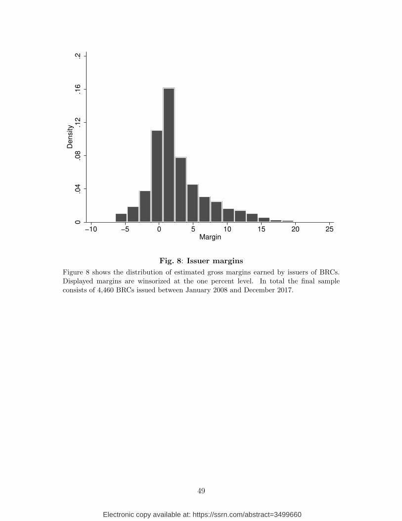
Fig. 8: Issuer margins

Figure 8 shows the distribution of estimated gross margins earned by issuers of BRCs.Displayed margins are winsorized at the one percent level. In total the final sampleconsists of 4,460 BRCs issued between January 2008 and December 2017.

49


0 2 4 6 8 10

Risk preference

-80

-60

-40

-20

0

20

40

Su

bje

cts

ma

rgin

s f

or

Sin

gle

an

d M

ulti Single

Multi

Fig. 9: Subjects’ margins and risk preferences

Figure 9 shows the relation of subjects’ risk preferences and the average margin for Singles(blue) and Multis (red). Risk preferences are measured following Holt and Laury (2002).The blue line shows the linear fit for margins of Singles (β = −1.66, p-value = 0.02). Thered line shows the linear fit for margins of Multis (β = −2.61, p-value < 0.01).

50


0 0.2 0.4 0.6 0.8 1

Overconfidence

-80

-60

-40

-20

0

20

40

Su

bje

cts

ma

rgin

s f

or

Sin

gle

an

d M

ulti Single

Multi

Fig. 10: Subjects’ margins and overconfidence

Figure 10 shows the relation of subjects’ overconfidence and the average margin for Singles(blue) and Multis (red). Overconfidence is measured according to the interval productiontask by Alpert and Raiffa (1982). Subjects are confronted with 10 knowledge questions.For each question, they are asked to provide a 90% confidence interval. A value of 1 meansthat a given subject’s intervals did not contain the true answer any of the ten questions.The blue line shows the linear fit for margins of Singles (β = 9.58, p-value = 0.24). Thered line shows the linear fit for margins of Multis (β = 18.95, p-value = 0.02).

51


Table 12: Product characteristics of all BRCs in the datasetTable 12 reports summary statistics of product characteristics at issuance for all BRCs in the

dataset. Coupon p.a. (in percent) is the product annual coupon rate extracted from its payoff

description. Barrier level (in percent) is the barrier level of the product when the put option gets

activated. Maturity (in days) is the maturity of a product. Number of underlyings indicates the

number of underlying assets that determine the final payoff of a product.

Panel A: Product characteristics

Mean Std Min Q1 Median Q3 Max

Coupon p.a. 8.70 3.67 0.20 6.15 8.00 10.26 57.34

Barrier level 67.19 9.35 30.00 60.00 69.00 75.00 93.00

Maturity 392.12 177.03 60 357 359 386 1,821

Number of underlyings 2.25 1.07 1 1 3 3 14

Observations 47,080

52


Table 13: Overview of structured products sample

Table 13 presents the number of issued structured products in our sample for both product types

grouped by issuer (Panel A) and year (Panel B). The subsample of Singles (Multis) consists of

2,528 (1,932) products. The total sample consists of 4,460 products issued between January 2008

and December 2017.

Panel A: By issuer

Single Multi

Vontobel 1,282 493

Julius Bar 659 217

EFG 158 137

Leonteq 133 312

CLEU 80 75

Credit Suisse 64 332

ZKB 31 88

HSBC 25 1

UBS 22 99

J.P. Morgan 18 20

BCV 14 12

Panel B: By year

Single Multi

2008 68 27

2009 114 38

2010 142 101

2011 246 143

2012 283 158

2013 295 147

2014 373 267

2015 335 240

2016 317 328

2017 355 483

53


Table 14: Closed form and simulated prices

Table 14 reports statistics of prices from the closed form solution and the Monte Carlo procedure,

respectively. The results of the Monte Carlo procedure are based on 365 time steps within a

year and 50,000 simulations per product. Marginclosed denotes the margins from the closed form

pricing model. Marginsimulated denotes the margins from the Monte Carlo procedure. The small

differences between closed form and simulated prices are due to the lower probability of a barrier

event, i.e., the activation of the embedded put option, implied by the latter’s discretization error.

Mean Std p2.5 Q1 Median Q3 p97.5

Marginclosed 2.10 4.51 -1.767 1.047 1.449 3.158 8.921

Marginsimulated 2.01 4.49 -1.844 0.972 1.377 3.081 8.769

Observations 2,528

54


Table 15: Underlying equities

Table 15 reports the 30 most frequent underlying assets used for Singles (Multis) in the sample,

the number of products that are linked to them and their percentage share in the total sample.

The sample consists of 4,460 BRCs corresponding to 172 underlying assets.

Single Multi

Underlying # products % share Underlying # products % share

Microsoft 113 4.47 Microsoft 429 7.61

Caterpillar 108 4.27 Alphabet 365 6.48

General Electric 103 4.07 Coca Cola 272 4.83

Tesla 101 4.00 General Eletric 248 4.40

Pfizer 88 3.48 Newmont Mining 221 3.92

Facebook 81 3.20 Goldcorp 211 3.74

Intel 75 2.97 Facebook 205 3.64

Alphabet 63 2.49 McDonalds 200 3.55

Exxon Mobil 55 2.18 Intel 176 3.12

Twitter 53 2.10 Pfizer 174 3.09

Newmont Mining 52 2.06 Starbucks 169 3.00

Cisco 50 1.98 Caterpillar 165 2.93

Alibaba 49 1.94 Netflix 143 2.54

HP 44 1.74 Cisco 88 1.56

Goldcorp 42 1.66 Nike 87 1.54

Starbucks 42 1.66 IBM 78 1.38

IBM 41 1.62 Gilead Sciences 74 1.31

Coca Cola 35 1.38 Johnson & Johnson 63 1.12

McDonalds 34 1.35 Exxon Mobil 161 1.08

Netflix 34 1.35 Mondelez 61 1.08

Gilead Sciences 29 1.15 Celgene 52 0.92

United States Steel 28 1.11 Biogen 50 0.89

Johnson & Johnson 26 1.03 Tesla 50 0.89

Halliburton 26 1.03 Disney Walt 48 0.85

Nike 24 0.95 Twitter 47 0.83

Petroleo Brasileiro 22 0.87 Procter & Gamble 46 0.82

JP Morgan 21 0.83 Visa 45 0.80

Celgene 21 0.83 Nvidia 35 0.62

GoPro 21 0.83 Alibaba 34 0.60

Penney JC 20 0.79 Walt Mart Stores 32 0.57

55


Table 16: Risk aversion lottery pairs

Table 16 shows pairs of lottery choices for the elicitation of individuals’ risk aversion. The values

are adapted from Holt and Laury (2002) to measure individuals’ risk aversion. Lottery A and

Lottery B differ only in their payoffs. Prob. denotes the probability that the corresponding payoff

of that pair is selected. Payoff is the corresponding payout. The values in the last column (∆) are

calculated as the difference in expectation. While in the first rounds Lottery A pays in expectation

a higher payoff, this changes from pair 5 onwards

Lottery A Lottery B ∆

prob. payoff prob. payoff prob. payoff prob. payoff

10% 2.00 90% 1.60 10% 3.85 90% 0.10 1.165

20% 2.00 80% 1.60 20% 3.85 80% 0.10 0.83

30% 2.00 70% 1.60 30% 3.85 70% 0.10 0.495

40% 2.00 60% 1.60 40% 3.85 60% 0.10 0.16

50% 2.00 50% 1.60 50% 3.85 50% 0.10 -0.175

60% 2.00 40% 1.60 60% 3.85 40% 0.10 -0.51

70% 2.00 30% 1.60 70% 3.85 30% 0.10 -0.845

80% 2.00 20% 1.60 80% 3.85 20% 0.10 -1.18

90% 2.00 10% 1.60 90% 3.85 10% 0.10 -1.515

100% 2.00 0% 1.60 100% 3.85 0% 0.10 -1.85

56


Table 17: Variable definitionsTable 17 provides definitions of all variables used in this paper.

Variable name Description Source

Nominal value, N Value invested in the product at issuance with-

out any fees

Dataset

Coupon p.a., c Maximum premium p.a. in percent % Dataset

Maturity, T Life time of the product (in days) Dataset

Barrier level, K Barrier price / Strike price Dataset

Strike level, S0 Strike level is equal to the value of the underly-

ing asset at issuance

Dataset

Year Calendar year of issuance date Dataset

Issuer Company that issues the BRC Dataset

Risk-free rate, r OIS rate linearly interpolated from the two near-

est maturities

Bloomberg

Dividend yield, µ Historical dividend yield of the underlying asset

over the past 12 months

CRSP

Implied volatility, σ Implied volatility bi-linearly interpolated from

the four closes options with respect to the strike

price and the maturity

OptionMetrics

Ivy DB US

Correlation, ρ Correlation of logreturns of the underlying as-

sets over the past 12 months

CRSP

Margin IMpt =IPpt−FPpt

IPptPricing model

Product return Retpt = 1(T−t)

[ln(

PayoffpT

IPpt

)− rft(T − t)

]Calculated

Age Age of the subjects Experiment

Male Gender of the subjects Experiment

Risk preferences Subject’s risk preferences measured according to

the test of Holt and Laury (2002)

Experiment

Confidence measure Subject’s overconfidence measured according to

the production task of Alpert and Raiffa (1982)

Experiment

WTP Willingness-to-pay for a Single or a Multi Experiment

Misestimation Difference in the true probability of barrier event

and subject’s estimated probability

Experiment

57


Appendix C. Experimental Instructions

The complete set of instructions (including comprehension questions) for our laboratory

experiment follow on the next four pages.

58


1

DepartmentofBankingandFinancePlattenstrasse32

www.bf.uzh.ch

Welcome to the Finance-Lab!

Please read the following instructions carefully. Fully understanding the instructions will increase your chances of

achieving a higher number of bonus points for the final exam of the lecture “Environmental and Financial

Sustainability”. At the end of these instructions, you will find 3 control questions. We will also go through a short

training session before starting the experiment. However, please take the time to understand the instructions fully.

If you have any questions, please raise your hand and an experimenter will come over to help.

Task

In this experiment, you will have the opportunity to buy different financial products. Your goal is to maximize your

total wealth. The experiment consists of 12 independent rounds. Each round is divided into two stages.

At the beginning of each round, you will be provided with an initial amount of 140 ECU (experimental currency

units). During every round, you will have the opportunity to use your cash to buy one financial product or to invest

your money at the risk-free rate. The price of the product is not yet fixed. It will be determined by chance. You will

never have to spend more for a product than you are willing to. You may even be able to buy it for less. Here is

how it works:

Stage 1

At the first stage of each round, all participants receive the same public information about all products available

for purchase. This information will help you to determine the value of each product. To do this more easily, you

will first be asked to estimate each product’s value components. Then, for a given list of different prices, you have

to decide whether you want to buy the product or not. This procedure is carried out for all products. In summary,

it should help you to make better decisions.

After all participants have made their decisions, the computer randomly selects one product. Thereafter, the

computer randomly sets the price for the selected product. If this random price is less than or equal to your

willingness to pay for the selected product, you will purchase the product at that randomly determined price. In this

case, the randomly determined price gets deducted from your initial cash amount and the remainder is automatically

invested at the risk-free rate. In contrast, if the random price is higher than your willingness to pay for the selected

product, your entire initial cash amount is invested at the risk-free rate. However, if you prefer to invest your initial

cash amount at the risk-free rate, independently of the randomly determined price, you will always have the chance

to do so. Notice, the risk-free rate can change between rounds.

For example, if you are willing to buy the selected product for up to 110 ECU and the randomly determined price

turns out to be 105 ECU, you only have to pay 105 ECU in return for the product. The remaining 35 ECU (=140-

105) will automatically be invested at the current risk-free rate. If, however, the randomly determined price turns

out to be higher than 110 ECU, you will not acquire the product and your total initial cash amount is automatically

invested at the current risk-free rate.

59


2


www.bf.uzh.ch

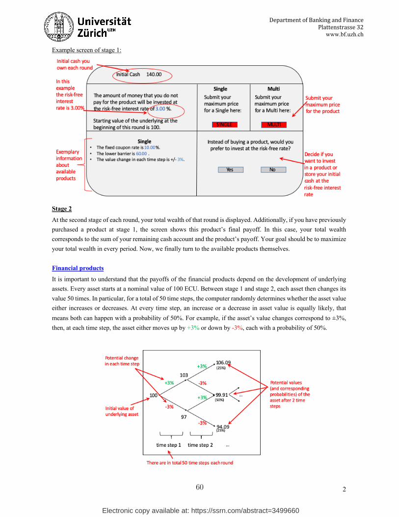
Example screen of stage 1:

Stage 2

At the second stage of each round, your total wealth of that round is displayed. Additionally, if you have previously purchased a product at stage 1, the screen shows this product’s final payoff. In this case, your total wealth corresponds to the sum of your remaining cash account and the product’s payoff. Your goal should be to maximize your total wealth in every period. Now, we finally turn to the available products themselves. Financial products

It is important to understand that the payoffs of the financial products depend on the development of underlying assets. Every asset starts at a nominal value of 100 ECU. Between stage 1 and stage 2, each asset then changes its value 50 times. In particular, for a total of 50 time steps, the computer randomly determines whether the asset value either increases or decreases. At every time step, an increase or a decrease in asset value is equally likely, that means both can happen with a probability of 50%. For example, if the asset’s value changes correspond to ±3%, then, at each time step, the asset either moves up by +3% or down by -3%, each with a probability of 50%.

60


3


www.bf.uzh.ch

There exist two different kinds of products:

Single:

A Single is a product whose final payoff depends on the development of 1 underlying asset with respect to a lower

barrier. Additionally, the product always offers a fixed coupon x (x% of 100 ECU) independently of the

development of the underlying asset. In total, the buyer’s payoff depends on the following two scenarios:

Scenario 1: If the underlying asset never hits the lower barrier, the buyer receives 100 ECU plus the guaranteed

fixed coupon x.

Scenario 2: If the underlying asset hits the lower barrier at least once, the buyer receives the lower amount of either

100 ECU or the final value of the asset, plus, in each case, the guaranteed fixed coupon x.

Multi:

A Multi is a product whose final payoff depends on the development of 2 independent underlying assets with

respect to a lower barrier. Additionally, the product always offers a fixed coupon x (x% of 100 ECU) independently

of the development of the 2 underlying assets. In total, the buyer’s payoff depends on the following two scenarios:

Scenario 1: If none of the 2 underlying assets hits the lower barrier, the buyer receives 100 ECU plus the guaranteed

fixed coupon x.

Scenario 2: If at least 1 of the 2 underlying assets hits the lower barrier at least once, the buyer receives the lower

amount of either 100 ECU or the worst performing underlying asset, plus, in each case, the guaranteed

fixed coupon x.

The expected payoff for both product types can always be decomposed into the following 4 components:

Expected payoff = Prob( Barrier hit ) * expected payoff( Barrier hit ) + Prob( Barrier not hit ) * payoff( Barrier not hit )

Example screen of stage 2:

61


4


www.bf.uzh.ch

Bonus points: You are guaranteed to earn 0.5 bonus points for participating in this experiment. Besides, you can

gain additional bonus points based on your investment decision. You can infer from the distributed table, how many

ECUs in a given round correspond to how many bonus points. At the end of the experiment, only one of the 12

independent rounds will be randomly selected. Your total wealth from this round will then be converted into bonus

points and credited to you at the final exam.

Please answer the following 3 comprehension questions:

1) Your initial cash amount is 140 ECU. The computer has randomly selected the Single and randomly set

its price equal to 100 ECU. The risk-free interest rate is 20%. Assume you are willing to pay 95 ECU for

the Single. What is your total wealth at the end of this period in ECU?________________

2) Assume the following development of the asset underlying a Single:

Which scenario has realized? Scenario 1 Scenario 2

3) Assume the following development of the assets underlying a Multi:

Which scenario has realized? Scenario 1 Scenario 2

******************************************************************************************* You will now go through a short training session to get familiar with the task. This training session will not impact

your bonus points.

50

60

70

80

90

100

110

120

0 10 20 30 40 50

valu

e

time step

barrier

asset

50

60

70

80

90

100

110

120

130

0 10 20 30 40 50

valu

e

time step

barrier

asset 1

asset 2

62


Date post:	23-Mar-2022
Category:	Documents
Upload:	others
View:	4 times
Download:	0 times

Structured Finance and Correlation Risk

Documents