Structured Peer-to-Peer Systems || Hierarchical Neighbor Maintenance

Chapter 3Hierarchical Neighbor Maintenance

Abstract In flat DHTs, various kinds of arranging items occur very frequently,leading to tree-like structures and hierarchical routing schemes. Different existingproposals can be unified in the terms of hierarchy, and routing schemes are built intoa logical structure. There are certain design principles that define general directionsfor various hierarchical techniques to improve DHT routing. This chapter shows thatthe known routing efficiency of flat DHTs is due to hierarchical schemes in the localconstruction and maintenance of routing tables.

3.1 Introduction

Nodes exploit the small-world phenomena, the lookup paths form hierarchicalstructures—lookup path hierarchies. They support the existence of short paths andprovide effective hierarchical routing schemes with local information. A commoncase is routing within O(logN) hops. These schemes are applied in Symphony [31],eCAN [51], Chord [48], Pastry [45], Tapestry [55], Kademlia [33], Koorde [21],Distance-halving [36, 38], D2B [13], ODRI [30], and Broose [15]. Sections 3.2and 3.3 coin the corresponding design principles of small-world neighborhood andgeometrically progressive routing.

Many extensions of flat DHT designs apply appropriate arrangement ofneighbors for adapting to a global hierarchy that exists in the network. Nodeslocally optimize lookup hops—a key design principle in neighbor and routeselection [3,9,17,52,54], multipath routing [18,25,54], sybil-resistance routing [10],load balancing [47], and some others. Section 3.4 elaborates this principle of locallyadaptive selection.

The lookup path hierarchy provides every node with an effective way forcollecting and using knowledge about the network beyond the neighbors. It is adesign principle in neighbor-of-neighbor routing [32,37], distributed trie of popularlookups [14], and cyclic routing [25]. Section 3.5 considers the DHT designs thatfollows the look-ahead principle.

D. Korzun and A. Gurtov, Structured Peer-to-Peer Systems: Fundamentals of HierarchicalOrganization, Routing, Scaling, and Security, DOI 10.1007/978-1-4614-5483-0 3,© Springer Science+Business Media New York 2013

47

48 3 Hierarchical Neighbor Maintenance

This principle evolves to DHTs with large routing tables or with high replication,when more expensive global routing is replaced with faster local routing by the costof node state and maintenance. The DHT family with large routing tables includesEpiChord [27], Accordion [29], SmartBoa [20], OneHop [12], 1h-Calot [49], andD1HT [34]. The DHT family with high replication is represented by DHash [8],Beehive [41], and Yarqs [53]. Sections 3.6 and 3.7 discuss these DHT families andthe problems they are faced with.

Recall from Chap. 1 that DHT routing construct multi-hop paths

u → w1 → w2 → ··· → wl−1 → d (3.1)

from a source node u = w0 to a responsible node d = wl . A widespread strategy isprogressive routing when (3.1) satisfies

ρ(wi,k)< ρ(wi−1,k), i = 1,2, . . . , l − 1. (3.2)

It leads to greedy routing in the extreme case:

wi = arg minu∈Twi−1

ρ(u,k), i = 1,2, . . . , l − 1. (3.3)

3.2 Small-World Networks and Progressive Routing

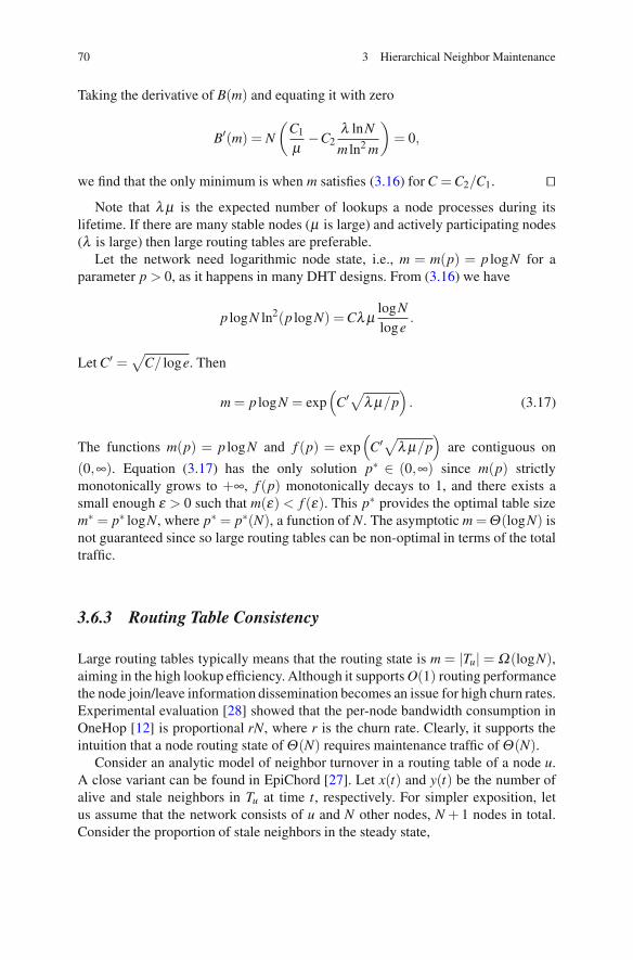
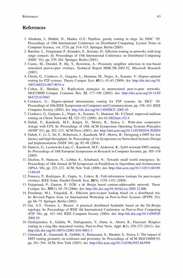
Models for the small-world phenomenon naturally exhibit a certain hierarchy inrouting tables. First, a node divides its neighbors onto local and long-range [23], inaccordance with the classifying model. Figure 3.1 shows the basic scheme. Localneighbors of a node u are equal. Long-range neighbors are arranged in u’s vicinity,in accordance with the ranking model.

3.2.1 Long-Range Neighbors

Kleinberg’s small-world construction [22] highlights the idea of selection distantnodes for neighbors. The node ID space is the n× n grid

u

local neighbors long−range neighbors ρ

Fig. 3.1 The small-world hierarchy of neighbors: (1) discrete classification onto local and long-range; (2) arrangement of long-range neighbors with vicinity clustering at all distance scales

3.2 Small-World Networks and Progressive Routing 49

S = {1,2, . . . ,n}×{1,2, . . . ,n}with ρ ((x1,y1),(x2,y2)) = |x2 − x1|+ |y2− y1|,

where N ≤ n2. Local neighbors of u are all v such that ρ(u,v) ≤ ε for a universalconstant ε ≥ 1. Additionally, u selects m ≥ 1 long-range neighbors with probabilityproportional to [ρ(u,v)]−α for α ≥ 0 (a kind of Zipf-like or power-law distribution).The parameter α controls the density of long-range neighbors at all distance scales.When α = 0 the long-range neighbors are distributed uniformly. As α increases,they become more clustered. Effective greedy routing is possible for α = 2; pathsare polylogarithmic with the expected length O(log2 N).

The small-world hierarchy of node’s neighborhood invents the following DHTdesign principle.

Principle 1 (Small-world neighborhood). Neighbors are at all distance scales.More distant neighbors are sparser in a local routing table.

An example DHT that does not follow Principle 1 is CAN [42]. Recall thatthe CAN ID space is the unit n-dimensional Cartesian coordinate space [0,1)n

mod 1 (torus) with Euclidean distance, a continuous analog of Kleinberg’s small-world grid. The coordinate space is partitioned into hyper-rectangles (zones). Eachnode is responsible for a zone (for keys from this zone). Two nodes are neighbors(symmetrically) if their zones share an n− 1 dimensional hyperplane, hence thereare only local neighbors. (Their number is m′ = 2n.) Greedy routing takes O(nN1/n)hops, and paths are longer than polylogarithmic. Only if the dimension satisfiesn = Θ(logb N) for some b > 1 or a more aggressive asymptotic dependence n =Ω(logb N) then the state and routing complexity can achieve O(logN) bound.

Consider the following definition. It provides a family of routing strategies,including greedy routing. A hop u → v for k is called b-progressive (geometricallyprogressive with the ratio 1/b) if

ρ(v,k)≤ ρ(u,k)b

for b > 1. (3.4)

As a result, the current distance is reduced at least by b, so considered as efficient.1

As we shall see, many DHT designs with logarithmic-complexity routingachieves geometrically progressive routing by appropriate selection of long-rangeneighbors.

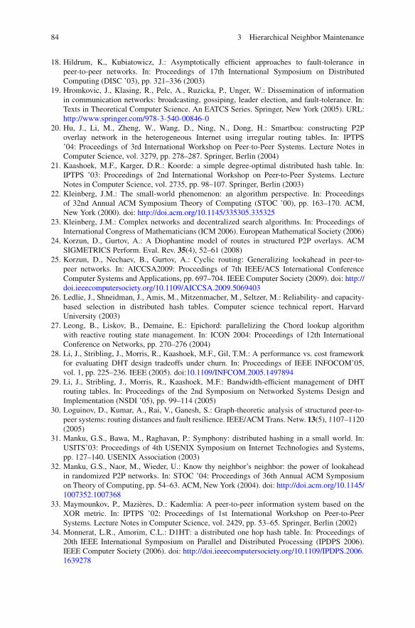
3.2.2 Case Study: Symphony

Symphony [31] is a particular inspiration of Kleinberg’s small-world construction.The ID space is a ring (the unit interval [0,1) mod 1). The distance ρ(u,k) is the

1In [52], such a routing strategy is called frugal; the corresponding paths are called geometric.


1/2

0

1/43/4

u likely zone forlocal neighbors

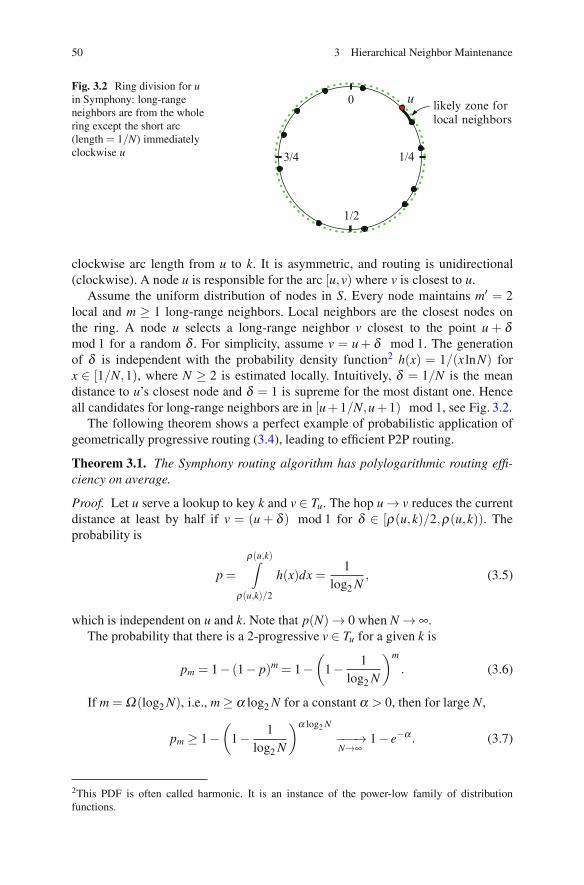
Fig. 3.2 Ring division for uin Symphony: long-rangeneighbors are from the wholering except the short arc(length = 1/N) immediatelyclockwise u

clockwise arc length from u to k. It is asymmetric, and routing is unidirectional(clockwise). A node u is responsible for the arc [u,v) where v is closest to u.

Assume the uniform distribution of nodes in S. Every node maintains m′ = 2local and m ≥ 1 long-range neighbors. Local neighbors are the closest nodes onthe ring. A node u selects a long-range neighbor v closest to the point u + δmod 1 for a random δ . For simplicity, assume v = u+ δ mod 1. The generationof δ is independent with the probability density function2 h(x) = 1/(x lnN) forx ∈ [1/N,1), where N ≥ 2 is estimated locally. Intuitively, δ = 1/N is the meandistance to u’s closest node and δ = 1 is supreme for the most distant one. Henceall candidates for long-range neighbors are in [u+ 1/N,u+ 1) mod 1, see Fig. 3.2.

The following theorem shows a perfect example of probabilistic application ofgeometrically progressive routing (3.4), leading to efficient P2P routing.

Theorem 3.1. The Symphony routing algorithm has polylogarithmic routing effi-ciency on average.

Proof. Let u serve a lookup to key k and v ∈ Tu. The hop u → v reduces the currentdistance at least by half if v = (u + δ ) mod 1 for δ ∈ [ρ(u,k)/2,ρ(u,k)). Theprobability is

p =

ρ(u,k)∫

ρ(u,k)/2

h(x)dx =1

log2 N, (3.5)

which is independent on u and k. Note that p(N)→ 0 when N → ∞.The probability that there is a 2-progressive v ∈ Tu for a given k is

pm = 1− (1− p)m = 1−(

1− 1log2 N

)m

. (3.6)

If m = Ω(log2 N), i.e., m ≥ α log2 N for a constant α > 0, then for large N,

pm ≥ 1−(

1− 1log2 N

)α log2 N

−−−→N→∞

1− e−α . (3.7)

2This PDF is often called harmonic. It is an instance of the power-low family of distributionfunctions.


For instance, pm ≈ 0.63 for m ≈ log2 N. That is, O(logN) routing state (typical tomany DHTs) leads to the high probability of geometrically progressive hops.

Consider a path wi →+ wi+1 with li hops where only the last one is at least2-progressive. Any forwarding node except the penultima has no 2-progressivehops in its routing table. A sufficient condition for the 2-progress is ρ(wi,k) ≥2ρ(wi+1,k). Note that in greedy routing a node always selects a geometricallyprogressive hop if it is available. The path hop length li is a random variable havingthe geometrical distribution

Pr[|wi →+ wi+1|= li

]= (1− pm)

li−1 pm

with the mean 1/pm. In addition, there are cases when the distance ρ(wi,k) is halvedby a sequence of short hops; it can only increase the probability of shorter pathswi →+ wi+1. In total, the expected length is E[li] = O(1/pm), which by (3.7) can bebounded above by a constant if N is large and m = Ω(log2 N).

For the fullness consider a less efficient strategy (in fact, the original proofin [31] used it) is the nodes on wi →+ wi+1 select the next hops randomly. Itconstructs longer paths before the current distance diminishes at least by half sincean intermediate node can have a 2-progressive hop but it was not selected. The pathconstruction also leads to geometrical distribution with the mean 1/p = log2 N:

Pr[|wi →+ wi+1|= li

]= (1− p)li−1 p.

The expected length E[li] = O(log2 N) by (3.5).Return to greedy routing case (3.6) in Symphony. Since p(N) tends to zero for

large N the expansion to Maclaurin series gives

pm = 1− (1− p)m = 1−∞

∑i=0

Cim(−1)i pi = mp+ o(p),

where Cim are generalized binomial coefficients. Consequently, the general bound is

E[li] = O(

log2 Nm

).

Now consider routing from the source node w0 to the responsible node d = wl

w0 →+ w1 →+ · · · →+ wl−1 →+ wl = d. (3.8)

Compared with (3.1), it consists of multi-hop subpaths wi →+ wi+1. Every subpathat least halves the distance. Hence Nwik < N/2i, and after l = O(log2 N) stepsNwl k = 0. Therefore, the Symphony greedy routing algorithm constructs paths ofthe expected length lE[li], and two important cases for node state complexity are

E[|u →+ d|]=

⎧⎨⎩

O

(1m

log2 N

)if m = O(1),

O(logN) if m = Ω(logN).

(3.9)

�


u

............ . . . . . .

. . .

d

1 3

2

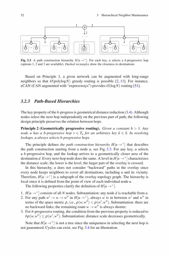
Fig. 3.3 A path construction hierarchy H[u →+]. For each key, u selects a b-progressive hop(options 1, 2 and 3 are available). Dashed rectangles show the closeness to destinations

Based on Principle 1, a given network can be augmented with long-rangeneighbors so that O(polylogN) greedy routing is possible [2, 11]. For instance,eCAN (CAN augmented with “expressways”) provides O(logN) routing [51].

3.2.3 Path-Based Hierarchies

The key property of the b-progress is geometrical distance reduction (3.4). Althoughnodes select the next hop independently on the previous part of path, the followingdesign principle preserves the relation between hops.

Principle 2 (Geometrically progressive routing). Given a constant b > 1. Anynode u has a b-progressive hop v ∈ Tu for an arbitrary key k ∈ S. In resolvinglookups, u always selects b-progressive hops.

The principle defines the path construction hierarchy H[u →+] that describesthe path construction starting from a node u, see Fig. 3.3. For any key, u selectsa b-progressive hop, and the lookup arrives to a geometrically closer area of thedestination d. Every next-hop node does the same. A level in H[u →+] characterizesthe distance scale; the lower is the level, the larger part of the overlay is crossed.

In this hierarchy, u does not consider “backward” paths in the overlay sinceevery node keeps neighbors to cover all destinations, including u and its vicinity.Therefore, H[u →+] is a subgraph of the overlay topology graph. The hierarchy islocal since it is defined from the point of view of each individual node u.

The following properties clarify the definition of H[u →+].

1. H[u →+] consists of all N nodes. Substantiation: any node d is reachable from u.2. For any path w′ → w → w′′ in H[u →+], always w is in between w′ and w′′ in

terms of the space metric ρ , i.e., ρ(w,w′′) < ρ(w′,w′′). Substantiation: there areno backward links; the remaining route w → w′′ is always shorter.

3. For b-progressive routing, the condition from the previous property is reduced tobρ(w,w′′)≤ ρ(w′,w′′). Substantiation: distance scale decreases geometrically.

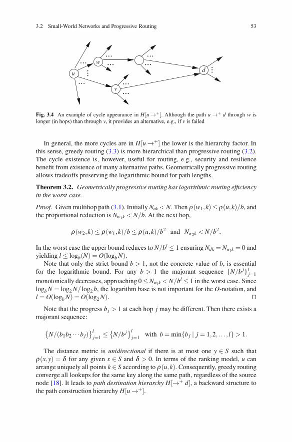
Note that H[u →+] is not a tree since the uniqueness in selecting the next hop isnot guaranteed. Cycles can exist, see Fig. 3.4 for an illustration.


... ...

...

......... ...

...

...

...u

v

dw

Fig. 3.4 An example of cycle appearance in H[u →+]. Although the path u →+ d through w islonger (in hops) than through v, it provides an alternative, e.g., if v is failed

In general, the more cycles are in H[u →+] the lower is the hierarchy factor. Inthis sense, greedy routing (3.3) is more hierarchical than progressive routing (3.2).The cycle existence is, however, useful for routing, e.g., security and resiliencebenefit from existence of many alternative paths. Geometrically progressive routingallows tradeoffs preserving the logarithmic bound for path lengths.

Theorem 3.2. Geometrically progressive routing has logarithmic routing efficiencyin the worst case.

Proof. Given multihop path (3.1). Initially Nuk < N. Then ρ(w1,k)≤ ρ(u,k)/b, andthe proportional reduction is Nw1k < N/b. At the next hop,

ρ(w2,k)≤ ρ(w1,k)/b ≤ ρ(u,k)/b2 and Nw2k < N/b2.

In the worst case the upper bound reduces to N/bl ≤ 1 ensuring Ndk = Nwl k = 0 andyielding l ≤ logb(N) = O(logb N).

Note that only the strict bound b > 1, not the concrete value of b, is essentialfor the logarithmic bound. For any b > 1 the majorant sequence {N/b j}l

j=1

monotonically decreases, approaching 0 ≤ Nwl k < N/bl ≤ 1 in the worst case. Sincelogb N = log2 N/ log2 b, the logarithm base is not important for the O-notation, andl = O(logb N) = O(log2 N). �

Note that the progress b j > 1 at each hop j may be different. Then there exists amajorant sequence:

{N/(b1b2 · · ·b j)

}lj=1 ≤

{N/b j}l

j=1 with b = min{b j | j = 1,2, . . . , l}> 1.

The distance metric is unidirectional if there is at most one y ∈ S such thatρ(x,y) = δ for any given x ∈ S and δ > 0. In terms of the ranking model, u canarrange uniquely all points k ∈ S according to ρ(u,k). Consequently, greedy routingconverge all lookups for the same key along the same path, regardless of the sourcenode [18]. It leads to path destination hierarchy H[→+ d], a backward structure tothe path construction hierarchy H[u →+].


d

.

.

.

. . .. . ....

layer 1

layer 2

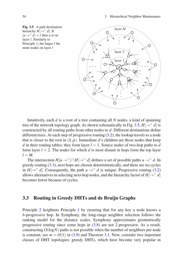
MlayerFig. 3.5 A path destinationhierarchy H[→+ d]. If|u →+ d|= l then u is onlayer l. Similarly toPrinciple 1, the larger l themore nodes on layer l

Intuitively, each d is a root of a tree containing all N nodes, a kind of spanningtree of the network topology graph. As shown schematically in Fig. 3.5, H[→+ d] isconstructed by all routing paths from other nodes to d. Different destinations definedifferent trees. At each step of progressive routing (3.2), the lookup travels to a nodethat is closer to the root in (S,ρ). Immediate d’s children are those nodes that keepd in their routing tables; they form layer l = 1. Source nodes of two-hop paths to dform layer l = 2. The nodes for which d is most distant in hops form the top layerl = M.

The intersection H[u →+]∩H[→+ d] defines a set of possible paths u →+ d. Ingreedy routing (3.3), next hops are chosen deterministically, and there are no cyclesin H[→+ d]. Consequently, the path u →+ d is unique. Progressive routing (3.2)allows alternatives in selecting next-hop nodes, and the hierarchy factor of H[→+ d]becomes lower because of cycles.

3.3 Routing in Greedy DHTs and de Bruijn Graphs

Principle 2 heightens Principle 1 by ensuring that for any key a node knows ab-progressive hop. In Symphony, the long-range neighbor selection follows theranking model for the distance scales. Symphony approximates geometricallyprogressive routing since some hops in (3.8) are not 2-progressive. As a result,constructing O(logN) paths is not possible when the number of neighbors per nodeis constant, see m = O(1) in (3.9) and Theorem 3.1. Now, consider two importantclasses of DHT topologies: greedy DHTs, which have become very popular in

3.3 Routing in Greedy DHTs and de Bruijn Graphs 55

Table 3.1 Popular greedy DHTs that employ geometrically progressive routing

DHT design ID space S Distance metric ρ(u,k)

Chord [48] n-bit numbers uniformlyprojected to the ring (b = 2)

ρ(u,k) ={

k−u, if u ≤ k,2n − (u− k), otherwise.

Clockwise arc length between u and k

Tapestry [55] n-digit numbers in base b ≥ 2 ρ(u,k) =n−1∑j=0

|u j − k j|b j where

u =n−1∑j=0

u jb j and k =n−1∑j=0

k jb j . Longer

the prefix (in digits) shared among uand k, closer these IDs

Pastry [45] Similarly to Tapestry withb = 2c for c ≥ 1

The same as in Tapestry

Kademlia [33] Similarly to Tapestry with b = 2 The same as in Tapestry. Equivalent tothe bitwise exclusive OR (XOR),

ρ(u,k) =n−1∑j=0

(u j ⊕ k j)b j

practical implementations, and de Bruijn P2P networks, which approximates deBruijn graphs in the topology. For these classes, the design can follow Principle 2accurately.

3.3.1 Conventional Greedy DHTs

Many DHTs with greedy routing use the classifying model (discrete) for neighbors,instead of the ranking model (continuous, ranks reflect the distance). As a result,routing becomes geometrically progressive. Examples include Chord [48], Pastry[45], Tapestry [55], and Kademlia [33].

Recall that the above DHTs use ID space S consisting of all nonnegative integerswith n ≥ 1 digits in base b ≥ 2, u = ∑n−1

j=0 u jb j for 0 ≤ u j < b, and N ≤ bn (seeTable 3.1). A node u discretely partitions S onto disjoint zones

Si(u) ={

k ∈ S | bi ≤ ρ(u,k)< bi+1} , i = 0, . . . ,n− 1. (3.10)

According to Principle 1, more distant zones are larger. In terms of the distance ρ ,each Si(u) is an annulus Bbi+1(u)\Bbi(u), the area between the two concentric balls,where an r-radius ball with center u is defined

Br(u) = {k ∈ S | ρ(u,k)< r} .

In Pastry and Tapestry, u keeps b− 1 long-range neighbors from each zone. Foreach Si(u), there is a neighbor v satisfying ρ(v,k) ≤ bi−1 for any k ∈ Si(u). Letus make explanation in terms of ID prefixes [40]. If v ∈ Si(u) then v, u and any


k ∈ Si(u) share the (n− i−1)-digit prefix. For each of b−1 values for the next digitj = 0,1, . . . ,b− 1, j �= un−i−1 that can follow this prefix in k ∈ Si(u), a long-rangeneighbor v ∈ Si(u) is stored in Tu. A lookup for k finds v ∈ Tu such that v is one digitcloser to k, i.e., ρ(v,k)≤ bi−1, and the hop is b-progressive:

ρ(u,k)ρ(v,k)

≥ bi

bi−1 = b.

In Chord and Kademlia, u keeps at least one long-range neighbor from eachzone. In Kademlia, the distance ρ is symmetrical, thus ρ(v,k) < 2i+1 − 2i = 2i forany k ∈ Si(u) and ith neighbor v. In Chord, the distance metric is asymmetrical. Indeterministic Chord the ith neighbor v is closest to u in Si(u), thus also ρ(v,k)< 2i

for any k ∈ Si(u). In routing a lookup, u uses the ith neighbor v. The hop u → v isgeometrically progressive since ρ(u,k)/ρ(v,k)> 1.

The Chord distance metric is transitive; ρ(u,k) = ρ(u,v) + ρ(v,k) if v is inbetween u and k. Without loss of generality, the latter can always be assumed fordeterministic Chord. Hence, having one ith neighbor ensures the 2-progress fordeterministic Chord:

ρ(u,k)ρ(v,k)

=ρ(u,v)+ρ(v,k)

ρ(v,k)≥ 2i

2i+1 − 2i + 1 = 2.

In randomized Chord as well as in Kademlia, v can be any node from Si(u), thus vis not always in between u and k.

For 2-progress in Kademlia, a node u would follow the same prefix-awarestrategy for selecting v ∈ Si(u) as in Pastry and Tapestry. Another way is halvingSi(u) and keeping two neighbors v1,v2 ∈ Si(u) for each half such that v1 and v2 areclosest to u in the annuli

B3·2i−1(u)\B2i(u) and B2i+1(u)\B3·2i−1(u), respectively.

Kademlia requires every u to keep several neighbors for each Si(u); the rec-ommended value is 20. Hence for a randomly selected k ∈ Si(u), the probabilityof having v ∈ Tu such that ρ(v,k) < 2i−1 is high. This strategy is also suitablefor randomized Chord, when some constant increment of the routing table sizeimproves the ratio of geometrically progressive routing.

As in the small-world construction, these greedy DHTs also support local neigh-bors: a list of successors in Chord,3 a leaf set4 in Tapestry, leaf and neighborhood5

sets in Pastry, nodes from S0 ∪Sn−1 in Kademlia.6

3A Chord node also keeps predecessors; they are local neighbors with respect to the absolutesymmetrical distance min{ρ(u,v),ρ(v,u)}.4A Tapestry or a Pastry leaf set consists of 2m0 numerically closest nodes (for the distance |v−u|):m0 clockwise plus m0 anticlockwise.5Pastry neighborhood set consists of proximity closest nodes.6In Kademlia (as in Chord) the closest successors of u are the first subsequent nodes in S0(u) andthe closest predecessors are the last subsequent nodes in Sn−1(u).


Summarizing, the considered greedy DHTs have the following properties.

1. Pastry and Tapestry ensures b-progressive routing by keeping b− 1 neighborsfrom each of n zones (m = O((b− 1) logb N) in total), where b is the base ofnumerical n-digit IDs.

2. Deterministic Chord ensures 2-progressive routing by keeping the closestneighbor from each power-two zone (m = n = O(log2 N) in total).

3. Randomized Chord and Kademlia ensure b-progressive routing for some b > 1by keeping at least one neighbor from each power-two zone. The probability thata hop is 2-progressive becomes higher when keeping more neighbors per zone.

3.3.2 Chord-Like DHTs

A Chord-like DHT is a generalization of the conventional Chord DHT by usingarbitrary base b ∈ Z, b ≥ 2, instead of the default base b = 2. The ID space can beseen as a discrete ring of bn points from 0 to bn − 1. A node takes its ID u ∈ [0,bn)and arithmetic on node IDs is always on modulo bn. The topology is constructed bylinks (fingers) that go from u to a node v∈ Si(u)= [u+bi,u+bi+1) for i= 0,1, . . . ,n.In deterministic topology, v is always the first node Si(u). In randomized topology,v can be taken arbitrary from Si(u). As a result, local state is O(logb N) and lookupcomplexity is O(logb N) hops. Note that a bidirectional variant is also possible whenadditional links (anti-clockwise fingers) from u to a node v ∈ Si(u) = [u− bi+1,u− bi) are maintained for i = 0,1, . . . ,n.

Intuitively, routing hops are “jumps” of size bi. The jump sizes σi = |Si(u)|= bi

are the same for at all nodes. In the terminology of Xu et al. [50] this property leadsto uniform routing algorithms. We will refer to the set {σi}n−1

i=0 as the jump set.Consider continuous generalization [50] when x ∈ R, 0 < x < 1. The jump set is{xi+1|S|}n−1

i=0 , where the number of neighbors n is selected such that xn|S| ≈ 1. Thediscrete case is reduced to the continuous one by taking x = 1/b.

The problem is to find a jump set that reduces the overlay network diameter. Letthe ID space be normalized into a unit interval [0,1), i.e., we move to the arithmeticon modulo 1. Then the jump sizes are σi = xi. The goal here is to approximateevery real number y ∈ [0,1) using these jump sizes in a “greedy” fashion, whenallowing a small “remainder”. This requirement is achieved by taking x =

√2−1≈

0.414, which is the root of the equation 1− 2x = x2. Given number y ∈ [0,1) toapproximate, there are three cases at the very beginning:

(a) If y ∈ [0,x) then the approximation is made.(b) If y ∈ [x,2x) then subtract x from it (a jump of size x in the normalized space)

and the remainder y− x is in [0,x).(c) If y ∈ [2x,1) then subtract x from it two times, and the remainder y− 2x is in

[0,x2).

The above procedure will be repeatedly executed in a recursive and greedyfashion. The intuition of the steps (a)–(c) is the following. If y belongs to case (a),


it is already “better-off” in terms of path length. If y belongs to case (b) or (c), thenone or two additional jumps of size x are needed to reduce the remainder to case (a).Since case (c) requires one more jump than case (b), we compensate this differenceby allowing its remainder to jump to the region [0,x2) (note that 1−2x= x2) insteadof [0,x) as in case (b). In this way, we “equalize” the cost to approximate numbersin regions [x,2x) and [2x,1). Note that such equalization is done in a recursive way,spreading its “equalization” benefit recursively.

The routing protocol is the same as in the original Chord. The number ofneighbors is reduced to n≈ log1/x N ≈ 0.786log2 N, which is 21.4 % less than in theoriginal Chord with the exactly log2 N routing table size. The average path length isapproximately 0.614log2 N, that is 22.7 % greater than in Chord.

Cordasco et al. [7] provided a further advanced scheme, called F-Chord(α).Its jump sizes are calculated based on Fibonacci numbers and 1/2 ≤ α ≤ 1 is atuning parameter. The model aims at better tradeoffs between overlay path lengthand routing table size.

Let fi be Fibonacci numbers for i = 0,1, . . ., which are defined as f0 = 0, f1 =1 and fi = fi−2 + fi−1 for i > 1. Fix n such that fn−1 < N ≤ fn. Note that m ≈logφ N ≈ 1.44log2 N, where φ = (1+

√5)/2 is the golden ratio. The basic idea

is that the difference between two consecutive jumps is the preceding jump, i.e.,σi+2 −σi+1 = σi. The maximum number of hops in greedy routing does not exceedhalf the size of the finger table. This basic case corresponds to α = 1. In general,F-Chord(α) uses the set of [α(n− 2)] jumps

σi =

{f2i, i = 1,2, . . . , [(1−α)(n− 2)],fi, i = 2[(1−α)(n− 2)]+ 2, . . .,n− 1,

where a certain quantity of the jumps with odd indices are eliminated.For any value of α , the diameter of an F-Chord(α) overlay network is half the

size of the routing table: [n/2]≈ 0.72log2 N, i.e., the worst-case path length is lowerthan in Chord. The average path length is upper bounded with

0.398log2 N +(1−α)0.248log2 N + 1.

The F-Chord(α) scheme can be further extended [6] to base b ≥ 2, where b isincreased in order to reduce the number of hops at the expense of increased routingtable size. It remains logarithmic in size, but the constant factor is higher.

3.3.3 De Bruijn Graphs

De Bruijn graph B(b,n) is a base for a rich family of DHT designs, includingKoorde [21], Distance-halving [36, 38], D2B [13], ODRI [30], and Broose [15].They also follows Principle 2 of geometrically progressive routing.


Fig. 3.6 The de Bruijn graphB(2,3); the picture isfrom [13]

As in greedy DHTs, the ID space S consists of n-digit nonnegative integers inbase b. The distance discretely depends on the length l(u,v) of the longest suffix ofu that equals the prefix of v,

l(u,v) = max{

j | u j−1=vn−1,u j−2=vn−2, . . . ,u0=vn− j},

where u = un−1 · · ·u1u0 and v = vn−1 · · ·v1v0. If the maximum does not exists thenl(u,v) = 0. For example, l(110,101) = 2, l(101,110) = 1, and l(011,001) = 0. Thelarger l(u,v), the closer the nodes. Therefore, l(u,v) follows the classifying modeland defines n distance scales.

Clearly, l(u,v) is not symmetric. Furthermore, if l(u,v) = l(u,w) then anadditional metric makes further differentiation. For instance, Koorde uses the Chorddistance, Distance-halving uses the absolute numerical difference, Broose uses theXOR distance as in Kademlia.

Similarly to the greedy DHTs, a node u partitions S onto several zones and selectsa neighbor for each of them. In contrast, the number of zones is equal to b withoutdependence on the ID length n, hence leading to O(1) state. Each zone Si(u) isdetermined by un−2un−3 · · ·u0i for i = 0,1, . . . ,b− 1, i.e., the node ID is shifted tothe left and appended with digit i on the right. The corresponding de Bruijn graphfor b = 2 and n = 3 is shown in Fig. 2.10 from Chap. 2.

In the greedy DHTs, each zone represents one distance scale. In the de Bruijngraph approach, Si(u) simultaneously covers all distance scales j = 0, . . . ,n − 1and is responsible for all keys k such that j = l(u,k) and the ( j+ 1)-digit prefix isu j−1 · · ·u0i. In routing a lookup for k = kn−1 · · ·k1k0, a node u computes j = l(u,k)and forwards to its neighbor v ∈ Skn− j(u), close to the point

un−2un−3 · · ·u ju j−1 · · ·u0kn− j−1

= un−2un−3 · · ·u jkn−1 · · ·kn− jkn− j−1

For the example in Fig. 2.10, the lookup for k = 101 at node s = 100 follows thepath 100 → 001 → 010 → 101.

The same neighbor is applicable at different distance scales; a lookup keydetermines what scale is needed. Nevertheless, Principle 1 is preserved since thenumber of nodes at distant scale j is proportional bn− j. Each routing step resolvesat least one digit in IDs, reducing the number of nodes in between at least by thefactor b in accordance with Principle 2.


The idea of geometrically progressive routing in de Bruijn graphs is furtherdeveloped in Kautz graphs, which we shall discuss in Sect. 4.7.

3.4 Adaptation to Global Hierarchy

Principle 1 is a base of small-world strategies for selecting neighbors. Its combi-nation with Principle 2 leads to discrete partitions on to distance-scale zones Si(u)in (3.10) and local hierarchies H[s →+] and H[→+ d] in the network topology. Inturn, this structure allows adapting to other hierarchies of the network. For instance,if the topology embeds a global hierarchy then the distance between two nodesdepends on the height of their lowest common ancestor in the hierarchy tree.

3.4.1 Kleinberg Tree-Based Model

First, consider an explaining theoretical example from [23]. Let the global hierarchybe represented as a complete b-ary tree T , where b is a constant (b ∈ Z+, b �= 0)and the height of T is logb N. The leaves are nodes N. For two leaves u and v, theheight of their least common ancestor in T is h(u,v). Clearly, h(u,u) = 0.

The network topology is stochastically adapted to the hierarchy as follows. Theprobability that u selects v a neighbor is equal to

puv =f (h(u,v))

∑w∈N,w �=u

f (h(u,w)), where f (h) = b−h.

It can be proved that the normalizing constant is bounded

∑w∈N,w �=u

f (h(u,w)) = ∑w∈N,w �=u

b−h(u,w) ≤ logb N.

According with this probability distribution, each u creates m links, choosing theneighbor v independently and with repetition allowed. Assume logarithmic nodestate m =Θ(log2

b N). Let us call this topology Kleinberg tree-based.7

The following theorem shows that structuring the topology using the tree-basedhierarchy allows efficient routing although every node has local knowledge only.

Theorem 3.3. A P2P network with Kleinberg tree-based topology allows a routingalgorithm that achieves O(logb N) efficiency with high probability.

7For m = O(1) the tree-based topology allows routing in O(log4b N) hops [23].

3.4 Adaptation to Global Hierarchy 61

Proof. Without loss of generality we assume that lookups are based on node IDsinstead of resource keys. Let u serve a lookup for the target node d. Suppose thatl = h(u,d) and t ∈ T is the least common ancestor. Let T ′ be subtree of T rootedat t and T ′′ be the subtree of T ′ of height l−1 that contains d. Obviously, u /∈T ′′.

If there is v ∈ Tu such that v ∈ T ′′ then u can make a b-progressive hop to d,achieving h(v,d) ≤ h(u,d)− 1. There are bl−1 leaves (network nodes) in T ′′. Forany v ∈ T ′′ the probability of being a neighbor of u is

pu = Pr{v ∈ Tu | v ∈ T ′′} ≥ b−l

logb N≥ 1

b logb N.

Since Tu = m ≥ C log2b N for a some constant C, the probability (1− pu)

m that Tu

contains no nodes from T ′′ is bounded for large N

(1− 1

b logb N

)m

≤(

1− 1b logb N

)C log2b N

≤ εC2 logb N = 1/N + o(1/N),

where 0 < ε < 1 and C2 > 0 are constants. Therefore, Tu contains a node from T ′′with high probability.

Then the required algorithm states each node u on the routing path to d to selectv ∈ Tu such that v ∈ T ′′, where T ′′ depends on u and d. From the foregoing itfollows that such v is in Tu with high probability.

No explicit construction of T ′′ is needed since u can select v that satisfiesh(v,d)< h(u,d). In the worst case, h(u,d) = logb N. Each hop reduces this discretedistance at least by 1, so the target is reached in O(logb N) hops. �

3.4.2 Proximity-Based Selection

Now consider the crucial practical instance of global hierarchy—the underlyingnetwork topology. It reflects the domain-based Internet architecture. The hierarchydefines the proximity of nodes in terms of latency. The height of their lowest com-mon ancestor of u and v positively correlates with the latency of communicationsbetween u and v. Let τ(u,v) be a latency metric estimated at u [39]. The latency ofl-hop path (3.1) is

|u →+ d|τ =l−1

∑i=0

τ(wi,wi+1).

An obvious property of geometrically progressive routing is the worst case bound

|u →+ d|τ = O(Δ logN) for the latency diameter Δ = maxu,v∈N

τ(u,v). (3.11)


Neighbor and route selection schemes (PNS and PRS) are known for adapting tothe proximity [3,9,17,29,52,54]. In PNS, a node u selects neighbors to Tu based ontheir proximity. In PRS, u selects next-hop nodes from Tu based on their proximity.The schemes aim at short paths not just in terms of overlay hops but also in termsof network latency. The aim is achieved with local optimization of latency at eachhop. As a result, the property τ(wi,wi+1)� Δ happens frequently in paths (3.1).

We treat PNS and PRS the concrete instances of the next design principle. Itapplies the ranking model where τ characterizes “node ranks” based on the globalhierarchy.

Principle 3 (Locally adaptive selection). Each node u locally arranges othernodes according to τ . In neighbor selection, u finds v that minimizes τ(u,v) ata given distance scale (defined by ρ). In routing, the selection of next hops usescomposite criteria with τ(u,v) and ρ(u,v).

DHTs with geometrically progressive routing can be modified to followPrinciple 3. In geometrically progressive routing, a node u keeps a neighbor foreach distance-scale zone (3.10). Randomized strategies allows selection amongseveral candidates in Si(u), giving the flexibility that PNS requires. Let u probemi > 1 nodes {v j}mi

j=1 from each distance-scale zone Si(u) and select the long-rangeneighbor with lowest τ(u,v j). Probing all nodes in Si(u) is enormously expensive,and mi is a tradeoff parameter.

The PNS scheme introduces a new hierarchy level when u additionally arrangesnodes in Si(u) according to the proximity. In routing a lookup for k, the next-hopnode v is proximity closest to u among all geometrically progressive neighbors.

There are networks where the worst case in (3.11) can be approached closelydespite the use of PNS. We say that the network has exponential latency expansionif for any u ∈ N

Nt(u) = |{v ∈ N | τ(u,v)≤ t}|=Θ(αt) for a constant α > 1.

In other words, the number of nodes that are within latency t of u growsexponentially.

Theorem 3.4. If a network has exponential latency expansion, then the expectedlatency E[|u →+ d|τ ] = Ω(Δ logN) for b-progressive paths u →+ d with nodesu,d ∈ N chosen at random.

Proof (Sketch, other details can be found in [52]). Take a random node w ∈ N. Withthe assumption on uniform node ID distribution in S, the set Si(w) itself is chosenuniformly at random from all subsets of N of size bi+1 − bi = (b− 1)bi, wherei = 0,1, . . . ,n− 1. Recall that N ≤ bn and for large N we assume n =Θ(logb N).

From the property of exponential latency expansion one can derive that

τi(w) = E [τ(w,v) | v ∈ Si(w)] ≥CiΔ (1− i/n) for a constant Ci > 0,

where τi(w) is the expected latency between w and Si(w).

3.4 Adaptation to Global Hierarchy 63

Given path (3.1) with random u,d ∈ N. Without loss of generality, if the path isb-progressive then assume l = n and wi+1 ∈ Sn−i−1(wi). Consequently,

E[|u →+ d|τ

]=

n−1

∑i=0

τi(wn−1−i)≥C′nΔ − C′′

n

n−1

∑i=0

i = Ω(Δ logb N). �

Theorem 3.4 means that no significant latency improvement is possible dueto PNS with probing mi nodes from each zone Si(u), especially when mi orSi(u) are small. Intuitively, in a network with exponential latency expansion, anoverwhelming majority of the nodes will be very far from u, and finding the closestnode from a small sample is unlikely to significantly improve the latency.

Now, let a network have power-law latency expansion:

Nt(u) = |{v ∈ N | τ(u,v)≤ t}|=Θ(tα) for a constant α ≥ 1.

In contrast to networks of exponential latency expansion, a network of power-law latency expansion ensures that a node u only needs to sample a small numberof nodes from each Si(u) in order to find a latency-nearby node.

Theorem 3.5. If a network has α-power-law latency expansion, then applying PNSwith m probes per zone Si leads to

E[|u →+ d|τ ] = O

(Δ

m1/α logN

)

for b-progressive paths u →+ d with nodes u,d ∈ N chosen at random.

Proof (Sketch, other details can be found in [52]). Let us define the minimal latencyfrom a node w ∈ N to a set of nodes V ⊂ N:

τ(w,V ) = minv∈V

τ(w,v).

Then one can prove that considering all random V of fixed size p ≥ 1, the expectedlatency is E[τ(w,V )] = O(Δ p−1/α). It asserts that the distance to the “closest” nodein V varies as p−1/α , a crucial consequence of α-power-law latency expansion.

Any w sampled a set S′i(w) ⊂ Si(w). For simplicity and ease of exposition, weassume8 that mi(w) = |S′i(w)| = m for all w and i. Given path (3.1) with randomu,d ∈ N. Without loss of generality, if the path is b-progressive then assume l = nand wi+1 ∈ S′n−i−1(wi). Consequently,

E[|u →+ d|τ

]=

n−1

∑i=0

τ(wn−1−i,S′i(wn−1−i))≤ Δ

n−1

∑i=0

Cim−1/αi = O

(Δ

m1/α logb N

).

�

8Without this assumption the proof becomes technically more complicated and an insignificantlymore precise upper bound E[|u →+ d|τ ] = O(Δ)+O

(Δm−1/α logN

)is derived, see [52].


Compared with (3.11) Theorem 3.5 provides the reduction by m1/α . Numerousexperimental studies confirmed the improvement significance in practical settings[3, 9, 17, 29, 52, 54]. Note that since

1

(m− 1)1/α − 1

m1/α ≥ 1

αm1+1/α ,

the improvement is most significant for the first few samples.Now consider the PRS scheme. It performs better if u knows many neighbors.

DHTs with geometrically progressive routing can support it by allowing u tokeep several nodes from each zone Si(u) if the node capacity is enough. (Notethat in Kademlia and Broose it is a principal design rule.) Then u arranges itsi-zone neighbors (already in Tu) according to the proximity. In routing a lookupfor k, composite criteria for selecting the next hop are applicable, e.g., the additivecriterion

cρ ρ(v,k)+ cττ(u,v)→ min (3.12)

for some tradeoff constants cρ ,cτ > 0. Minimizing ρ(v,k) preserves geometricallyprogressive routing within few overlay hops. Minimizing τ(u,v) makes each hop tobe of low latency.

For practical implementations the following simple algorithm can be suggested.It is approximate and separates the minimization on ρ and τ .

1. Given k, u finds m closest neighbors based on ρ ; denote the set Tu(k).2. The next hop is v = arg min

w∈Tu(k)τ(u,w).

On one hand, Tu(k) likely provides the best b-progress hops for k, preserving routingefficiency in hops. On the other hand, the proximity is taken into account, reducingthe latency. Note that in a network of α-power-low latency expansion, the expectedimprovement is latency reduction by m1/α , similarly to Theorem 3.5.

The hierarchical routing scheme with several neighbors from Si(u) also supportsmulti-path routing. A lookup is forwarded in parallel to several next hops. Signif-icantly better routing performance and resilience are possible, see comprehensiveexperiments in [15, 18, 25, 27, 29, 33, 51, 54]. For example, Kademlia exploits thisscheme to tolerate node failures. Every ith set of neighbors is kept sorted by timelast seen. In this case, τ(u,v) is the time elapsed from the last successful contactwith v.

3.4.3 Other Criteria for Local Adaptation

In general, Principle 3 supports arbitrary hierarchy-based metrics τ , not onlylatency-oriented. For instance, [10] adapts in the topology another practicalglobal hierarchy—the bootstrap tree B from social networking, used for a trustmetric. When joining to the network, a node u has to contact an existing node v

3.5 Global Routing and Lookup Structure 65

(the first contact). The knowledge of v is previous off-line relationship between uand v. The set of all relationships defines B. Each node u for each neighbor v storesadditionally (in Tu) the path from u to v in B.

The approach aims at secure routing (sybil-resistance) when an adversaryconvinces good nodes to allow it to join the network. Then the adversary introducesa large number of sybils via this attachment point. Assuming the complexity ofobtaining an attachment point is much higher than introducing sybils, B includesonly a small number of large subtrees of sybils. Consequently, there is a highprobability that a path of good nodes exists in B between any two good nodes.

Routing is iterative. A node u at each hop u → v receives from v the whole Tv,thus u can construct the path to any w ∈ Tv in B. Then u selects the appropriatenext hop. Similar to the case of proximity, the selection uses a trust metric τ(u,v)of the path from u to w in B (diversity routing). The various composite criteria areapplicable, convex

cρ(v,k)+ (1− c)τ(u,v)→ min for 0 ≤ c ≤ 1 (3.13)

or zig–zag (alternation of progressive and diversity routing)

cρ(v,k)+ (1− c)τ(u,v)→ min (3.14)

when each step alternates c = 0,1,0,1, . . .. Note that (3.13) is a particular case of(3.12); it needs to measure the distance ρ and trust τ in comparable units.

A global hierarchy can be related to the system load balance. For instance in [47],each node estimates the load of its neighbors and replaces the most loaded neighborswith other nodes. In this scheme, τ is proportional to the load inversion. The goalis minimizing the number of lookups forwarded to the nodes that owns popularresources (hot spots). The idea is evolved further to algorithms that group nodes forefficient load-balancing (see Chap. 4). Neighbor and route selection with τ reflectingnode reliability and capacity was introduced in [26].

3.5 Global Routing and Lookup Structure

Principle 3 allows each node to locally adapt to certain characteristics of a globalhierarchy defined by a metric τ . The latter is used for extrapolation of the localknowledge. Nevertheless, a node u would prefer additional more precise knowledgeabout the rest of path u → v →+ d beyond the hop u → v.

In progressive routing, the first hops in u →+ d are likely large in distance ρ .For instance, greedy routing tries at each hop to cross as large part of the overlay aspossible. Let us consider routing divided logically into global and local parts. Globalrouting delivers a lookup to destination vicinity. In local routing, the destination isat a nearby node.


According to Principle 1, a node knows its neighborhood rather well. First,many nearby nodes are local neighbors. Second, the lower distance scale the moreneighbors in a routing table. In this sense, local routing has more informationthan global routing. Therefore, global routing is an important subject for furtheroptimization based on additional knowledge. Principle 2 is mostly for global routingsince the geometrical reduction aims at large hops.

Principle 4 (Look ahead). A node utilizes additional knowledge about pathsbeyond its neighbors to optimize global routing.

Various hierarchical schemes can be defined on top of the path constructionhierarchies H[u →+] to keep (partially) the current lookup state. The examplesinclude neighbor-of-neighbor (NoN) routing [32, 37], distributed trie of popularlookups [14], and cyclic routing [25].

3.5.1 NoN-routing

Progressive routing is augmented with a lookahead mechanism. For routing deci-sions, u (in addition to its neighbor v) analyzes l subsequent nodes on paths

u → v∗ → w1 → ··· → wl →+ d. (3.15)

NoN-routing is greedy routing with lookahead for l = 1 [32, 37]. In a lookup for k,a node u knows nodes w ∈ Tv for any v∈ Tu. Note that IP addresses IPw are unknownto u, thus the maintenance overhead is low (no pinging). Among these w, the nodeu finds w1 ∈ Tv∗ closest to k and forwards the lookup to the corresponding v∗.

Likely, the lookup then goes to w1, reducing the distance more effectively thangreedy routing without lookahead. Note, however, that it is not guaranteed that v∗forwards the lookup exactly to w1 since v∗ makes own decision on the next hop.

NoN-routing exploits two levels in H[u →+]: neighbors v ∈ Tu (level i = 1) →neighbors-of-neighbors w ∈ Tv (level i = 2). It improves the routing performance inrandomized P2P networks [1, 32]. Symphony with NoN-routing achieves expectedpath length bound O(log2 N/(m logm)) with m long-range neighbors per node [32],i.e., the reduction factor is logm, see (3.9). Pappilon provides Θ(logN/ logm)routing in the worst case [1]. For many DHTs, Θ(logN/ log logN) routing isexpected [4, 32]. A NoN-routing scheme without additional overhead is introducedin [4]; it “limits” the randomization of the original scheme such that neighborhoodinformation is encoded within the hash-value of the node ID.

3.5.2 Distributed Trie

The lookup structure can be organized locally as a tree-like hierarchy that reflectsmost popular lookups [14]. Recall from Chap. 2 that a distributed trie utilizes the

3.5 Global Routing and Lookup Structure 67

same idea of prefix-matching routing [40] as in Pastry and Tapestry. In fact, Tu is atree of tables representing H[u →+]. A table consists of 2m entries, each containsseveral nodes as triples (v, IPv, t), arranging nodes by timestamps t (last recent seen).

Each level in Tu sequentially resolves m bits in the prefix of the n-bit key, leadingto paths in the tree as the following (n = 6, m = 2, k = 010010):

******→ 01****→ 0100**→ 010010

A non-leaf routing table contains nodes v known to resolve the next m bits at timet; the child routing tables contains the corresponding neighbors of v. An entry of aleaf routing table contains a node known at time t to be responsible for a key withthe sum prefix (constructed top-down from the root). Note that if a node v appearsin some routing table of Tu, then u keeps an entire path down to v.

In a lookup for k, u searches the tree Tu moving down to the leaf routing tablesthat keeps an entry for the longest prefix p of k. The entry contains a node v withthe latest timestamp, i.e., v is most recently known to u to hold the child routingtable, not currently available at u. Then, u requests v for either this table or, if v isresponsible for k, the resource.

Each node u exploits of the current lookup structure up to any level basedon lookups in which u has participated. Local representation Tu evolves in time.Frequent overlay paths are cached at u; the more popular and stable the resourceor node, the more efficient routing. It is expensive when churn is high or there aremany nodes with popular resources.

3.5.3 Cyclic Routing

Similarly to the distributed trie approach, Cyclic Routing (CR) provides a systematicway for collecting efficient paths up to any level of the lookup structure [24, 25].A cycle is a path that starts from the source node to its neighbor, then runs throughthe overlay and returns to the source:

u → v →+ w1 →+ · · · →+ wl →+ u.

Compared with l-lookahead (3.15), there can be intermediate nodes in wi →+ wi+1

that are not fixed explicitly. Hence, the CR selection of nodes to represent a givencycle is flexible and can be adapted to various routing requirements.

Each node u maintains a collection of cycles additionally to its primary routingtable Tu. As in NoN-routing, only node IDs are stored to identify a cycle. Inprogressive routing, u uses either cycles or the underlying DHT. If there is a cyclewith a node close to the key, the lookup is sent along the cycle. Otherwise, theunderlying DHT selects the next hop.

This strategy supports l-lookahead for any l ≥ 1 as well as takes the bidirectionalnature of P2P communications into account. The CR focus on global routing is


along the cycle

Local routing tothe destination

Neighborhood

Global routing

u

v

d

wl

wi

Fig. 3.7 A node u utilizesCR for better global routing.When a lookup appears in d’sneighborhood (a node wi),local routing is performed

emphasized in Fig. 3.7. Compared with the distributed trie, where all destinationsare strictly partitioned among paths in Tu, the same cycle can be used for manydestinations and different cycles can be used for the same destination. As a result,CR provides a rather compact data structure for the information about availablepaths. It can be used in any DHT with progressive routing. When the size oflocal collection of cycles grows then this local knowledge becomes an interpolationrather than extrapolation for the global network topology, and we defer the detailedanalysis of the CR method until Part III.

3.6 Routing with Large Routing Tables

Principle 4 states that u’s primary routing table can be augmented with additionalinformation from H[u →+] for better global routing. In the extreme case, this idealeads to O(1) routing with large routing tables. The difference between globaland local routing disappears, since the majority of nodes becomes in every node’sneighborhood. On the other hand, the maintenance cost can become high, asexperimental study [28] confirmed.

3.6.1 Designs with Large Routing Tables

For achieving O(1) routing (up to one-hop routing), upper limits for the routingtable size are removed, as appeared in EpiChord [27] and Accordion [29]. It leadsto systems with large routing tables, up to complete membership information.Extreme examples are OneHop [12], 1h-Calot [49], and D1HT [34] where everynode must keep a complete routing table; work [35] makes their comparison. Notethat SmartBoa [20] also utilizes large sizes for high-bandwidth nodes (see Sect. 4.4).

EpiChord [27] removes the O(logN) state upper bound of Chord using a reactiverouting state maintenance strategy that amortizes network maintenance costs intoexisting lookups and uses parallel lookups (multipath routing). The routing tablesize has no upper limit, and nodes adapt to a wide range of lookup workloads.EpiChord is able to achieve O(1)-hop routing under lookup-intensive workloadsand at least O(logN) routing under churn-intensive workloads.

3.6 Routing with Large Routing Tables 69

Accordion [29] adapts to current operating environments and node bandwidthbudgets. Nodes proactively search new neighbors. As in Symphony, the density ofits long-range neighbors is inversely proportional to the distance. Accordion is notbased on a particular data structure, and it has freedom in choosing the size andcontent of its routing table. The number neighbors m varies from O(logN) to O(N)states. The bandwidth budget controls the rate of learning about new neighbors.Each node limits its routing table size by evicting failed neighbors. The equilibriumbetween the learning and eviction processes determines the table size.

3.6.2 Maintenance Traffic Overhead

A comparison of DHTs with variable routing table sizes from O(1) to O(logN) isgiven in [49]. In particular, it introduced a model for the tradeoff between the routingtable size m = |Tu| and the total traffic generated in a network with logarithmicrouting complexity. In addition to N and m, the model parameters are lookup rateλ (workload) and node lifetime μ (churn). Note that r = 1/μ is the churn rate; inother words, r is the node turnover rate—a fraction of nodes that the churn replacesin the system per time unit.

Theorem 3.6. Given a P2P network with N nodes, equally fixed routing table sizem = |Tu| ∀u ∈ N, and the routing complexity of Θ(logm N) hops. Let λ and μ benode lookup rate and expected node lifetime, respectively. Then the minimum oftotal traffic is attained for m that is a solution to

m ln2 m =Cλ μ lnN, (3.16)

where C is a constant determined by the P2P protocol.

Proof. Since λ and μ are characteristics of the expectations, the subsequent resultsare also for an expected case. At any time instance, the network is preserved to be Nnodes in total, i.e., N/μ nodes leave and correspondingly N/μ nodes join per timeunit.

When a node joins or leaves, each of its m neighbors should be notified. Itrequires exchanging a constant portion of traffic per neighbor. Thus, the churn-related maintenance traffic is Bchurn = C1mrN. The constant C1 characterizes theP2P maintenance protocol.

Each alive node initiates λ lookups per time unit, resulting in λ N lookups intotal. The traffic for lookups is therefore Blookup = C2λ N logm N. The constant C2

characterizes the P2P routing protocol.The total traffic is the following function of m:

B(m) = Bchurn +Blookup = N(C1mr+C2λ logm N).


Taking the derivative of B(m) and equating it with zero

B′(m) = N

(C1

μ−C2

λ lnN

m ln2 m

)= 0,

we find that the only minimum is when m satisfies (3.16) for C =C2/C1. �Note that λ μ is the expected number of lookups a node processes during its

lifetime. If there are many stable nodes (μ is large) and actively participating nodes(λ is large) then large routing tables are preferable.

Let the network need logarithmic node state, i.e., m = m(p) = p logN for aparameter p > 0, as it happens in many DHT designs. From (3.16) we have

p logN ln2(p logN) =Cλ μlogNloge

.

Let C′ =√

C/ loge. Then

m = p logN = exp(

C′√λ μ/p). (3.17)

The functions m(p) = p logN and f (p) = exp(

C′√λ μ/p)

are contiguous on

(0,∞). Equation (3.17) has the only solution p∗ ∈ (0,∞) since m(p) strictlymonotonically grows to +∞, f (p) monotonically decays to 1, and there exists asmall enough ε > 0 such that m(ε) < f (ε). This p∗ provides the optimal table sizem∗ = p∗ logN, where p∗ = p∗(N), a function of N. The asymptotic m =Θ(logN) isnot guaranteed since so large routing tables can be non-optimal in terms of the totaltraffic.

3.6.3 Routing Table Consistency

Large routing tables typically means that the routing state is m = |Tu| = Ω(logN),aiming in the high lookup efficiency. Although it supports O(1) routing performancethe node join/leave information dissemination becomes an issue for high churn rates.Experimental evaluation [28] showed that the per-node bandwidth consumption inOneHop [12] is proportional rN, where r is the churn rate. Clearly, it supports theintuition that a node routing state of Θ(N) requires maintenance traffic of Θ(N).

Consider an analytic model of neighbor turnover in a routing table of a node u.A close variant can be found in EpiChord [27]. Let x(t) and y(t) be the number ofalive and stale neighbors in Tu at time t, respectively. For simpler exposition, letus assume that the network consists of u and N other nodes, N + 1 nodes in total.Consider the proportion of stale neighbors in the steady state,

3.6 Routing with Large Routing Tables 71

γ = limt→∞

y(t)x(t)+ y(t)

,

where |Tu|= x(t)+ y(t)≤ N.Form u’s point of view the rest network permanently consists of N nodes such

that Nrdt of the nodes are renewed uniformly at random due to churn in a timeinterval dt. At the same time interval, u detects a fraction νdt of stale nodes amongits neighbors and u removes them from Tu. Also, u makes λ dt lookups uniformlyover the ID space, as well as the other N nodes make their own lookups uniformlywith the same rate λ . Then we obtain the following differential equation for x(t):

dxdt

= λ (1− xN)− rx, (3.18)

where λ (1− x/N) is the number of incoming lookups to u from newly appearednodes (u makes them neighbors), rx is the number of the neighbors having becomestale in Tu (u still thinks that they are alive). Similarly,

dydt

= rx−νy, (3.19)

where νy is the number of stale neighbors that u removes from Tu.Equations (3.18) and (3.19) forms a system of first-order linear ordinary

differential equations. It similar in essence to continuous-time birth-death processes.The solution can be obtained analytically as a steady state and a time-dependentsum of terms with exponents exp(−αt) for α > 0. Hence the solution convergesquickly to the steady state solution, for which dx/dt = dy/dt = 0. It is a solution tothe following linear system:

λ − (r+λ/N)x = 0, rx−νy = 0, x+ y ≤ N.

It leads to

x =λ

r+λ/N, y =

λ rν(r+λ/N)

, γ =r

r+ν, where λ ≤ νN. (3.20)

Clearly, γ → 0 when the churn is reduced (r → 0) and γ → 1 when the churn grows(r → ∞ and ν = o(r)).

Outgoing lookups provides a way for u to detect stale neighbors in Tu. Forinstance, a neighbor is treated failed if there is no acknowledgment (in EpiChord).Another way is proactive pinging in background, when periodicity is proportionalto the lookup rate (in Accordion). In both cases, the detection rate is ν = cλ fora constant c > 0, leading to γ = r/(r + cλ ). The constant c can be increased withparallel lookups. The condition λ ≤ νN is satisfied for all N large enough.


1 4 72 3 5 6 98

failure

TTL=0 TTL=0 TTL=0 TTL=0 TTL=0TTL=1 TTL=1

TTL=2 TTL=3

v v vv v v v vvuw

Fig. 3.8 Nodes propagate an event using geometrically progressive hops with correspondingTTLs. If u detects that w is failed then u reports the event to its neighbors vi setting the eventmessage TTL proportionally to the distance. In turn, each vi decrements TTL and forwards themessage further. The event disseminated over all nodes in the logarithmic time and withoutduplicates

Theorem 3.7. Given an N-node network with churn rate r ≥ 0, lookup rate λ ≥ 0and stale node detection rate ν ≥ 0 such that λ ≤ νN. Then in the steady state:

1. The proportion γ of stale neighbors is independent on the network size N.2. The asymptotic for N → ∞ is x → λ/r and y → λ/ν .3. If ν ≥ r then γ ≤ 1/2 (at most half of the neighbors are stale if the stale node

detection is at least as fast as the node failure rate).4. If ν = cλ then y → 1/c for N → ∞ (the stale node detection that is proportional

to the lookup rate leads to the small number of stale neighbors).5. x= λ μ for N →∞ (the number of alive neighbors is equal to the expected number

of lookups that a node processes during its lifetime).

Proof. All the assertions are obvious consequences of (3.20). Assertion 5 uses thefact that the expected node lifetime is μ = 1/r. �

Assertions 2 and 5 show that large routing tables appear when λ , μ , or ν are high(cf. the similar conclusion after Theorem 3.6).

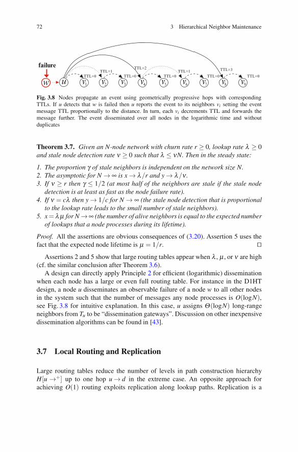
A design can directly apply Principle 2 for efficient (logarithmic) disseminationwhen each node has a large or even full routing table. For instance in the D1HTdesign, a node u disseminates an observable failure of a node w to all other nodesin the system such that the number of messages any node processes is O(logN),see Fig. 3.8 for intuitive explanation. In this case, u assigns Θ(logN) long-rangeneighbors from Tu to be “dissemination gateways”. Discussion on other inexpensivedissemination algorithms can be found in [43].

3.7 Local Routing and Replication

Large routing tables reduce the number of levels in path construction hierarchyH[u →+] up to one hop u → d in the extreme case. An opposite approach forachieving O(1) routing exploits replication along lookup paths. Replication is a

3.7 Local Routing and Replication 73

technique in which data are stored at multiple nodes of the network. For the basicquestions we address, it does not matter if the actual data is replicated or if onlypointers to the data are replicated.

Replication improves lookup performance and alleviates hot spots since a replicamay be found at a nearer node than the primary responsible node. The improvementdepends on the number of replicas and the placement strategy. The latter essentiallyexploits the network structure.

3.7.1 Source-Aware Replication

The extreme case is caching when after a successful lookup the query node storesa replica. For example, such a variant was suggested in CAN [42] where each nodecan maintain a cache of the resource keys it recently accessed (in addition to itsprimary store).

The next possible step is replication at neighbors. The generalization followsPrinciple 4: each node can look ahead in selecting appropriate nodes for replication.Plaxton et al. [40] apply the source-aware replication. Let u and k be a random nodeand key, respectively. One of the basic consequences of Plaxton’s model is that ifv is the nearest node to u that holds a replica (or original) resource for k then thelookup cost is proportional to l = |u →+ v|. Consequently, if interesting resourcesare replicated in u’s vicinity then the lookup performance of u is determined mostlyby local routing.

This idea can be implemented based on H[u →+]. If u made a lookup for k withpath (3.1) to d, then the resource with this key are replicated near u at r + 1 firstnodes w0, w1, . . . , wr. Then subsequent lookups for k are resolved more efficiently.Popular resources are targets of many users, spread over the overlay.

Consider an analytic model, assuming that all resources have the same popularity.Let u make a lookup for k, where u and k are taken at random. Let d be the primaryresponsible node for k and |u →+ d| = l. Assume that each node w0 = u, w1, . . . ,wr on the path u →+ d keeps a replica for k with probability pk. It characterizes thepopularity-based replication fraction of k relatively to u since u has already servedlookups for k and some nodes can still keep the replicas.

The probability that there is no node on u→+ d to resolve the lookup earlier thanreaching d is (1− pk)

r+1. In this case, the replication mechanism is not involved andthe lookup path length is l, e.g., l =Θ(logN). It decreases rapidly, especially whenpk is close to 1 (high popularity of k) or r is close to l − 1 (high replication factor).

With probability 1− (1− pk)r+1 the lookup path becomes of r hops or shorter.

The expectation is

E[Lk] =r

∑i=0

i(1− pk)i pk = pk

r

∑i=1

i(1− pk)i,


where (1 − pk)i pk is the probability that u = w0, w1, . . . , wi−1 have no replica

of k and wi keeps the replica. The sum can be reduced,9 yielding the followingimprovement to the expected lookup performance:

E[Lk] =1− pk

pk

(r(1− pk)

r+1 − (r+ 1)(1− pk)r + 1

). (3.21)

Theorem 3.8. Given an N-node network with source-aware replication factor r ∈Z+ and replication fraction pk ∈ [0,1] for some k ∈ R. Then the replication providesthe following improvement to the expected lookup performance for k

1. E[Lk]≤ (1− pk)/pk.2. E[Lk]→ 0 for pk → 1.3. E[Lk]→ (1− pk)/pk for large r.

Proof. Consider the function f (q,r) = rqr+1 − (r+ 1)qr for q = 1− p ∈ (0,1] andr ∈ [0,∞). The derivative is ∂ f/∂q = r(r + 1)qr−1(q− 1) < 0, thus f decreasesmonotonically for q and takes values in [−1,0). Applying (3.21) proves the firstassertion of the theorem.

The second assertion follows from the first one. Note also that the function y(x) =(1− x)/x is strictly decreasing on (0,1).

To prove the last assertion consider the derivative

∂ f∂ r

= qr ((rq− (r+ 1)) lnq− (1− q)).

It is positive for r large enough since the inequation (rq− (r+1)) lnq− (1−q)> 0has solutions r >−1/ lnq−1/(1−q). Let r0 = max{−1/ lnq−1/(1−q),0}. Thenf (q,r) increases monotonically for r ∈ (r0,∞) and f (q,r) ≈ 0 for large r. �

Note that the case with non-zero probability for the nodes wr+1, . . . , wl−1 alsoto replicate k allows further reduction of the lookup path length. Consequently, theabove model provides the upper bound. For instance, if k is popular, e.g., p > 1/2then with probability 1−1/2r+1 the resolution of a lookup for k takes 2 or less hops.

As a result of the source-aware replication, popular resources are replicated atmany nodes on all layers of H[→+ d] (see Fig. 3.5 in Sect. 3.2). If u’s neighbors,neighbor of neighbors, and so on are active in some resources then the search ofthese resources becomes more efficient for u. This replication strategy reduces theneed in global routing since the resource can be found by means of local routingwith O(1) lookup performance.

9Denote f (x) = ∑ri=1 ixi and g(x) = ∑r

i=1 xi+1. Then g′(x) = ∑ri=1(i + 1)xi = f (x) + 1−xr

1−x x. On

the other hand, g′(x) = x(1−x)2

((r+1)xr+1 − (r+2)xr − x+2

)since g(x) = 1−xr

1−x x2. We obtain

f (x) = g′(x)− 1−xr

1−x x = x(1−x)2

(rxr+1 − (r+1)xr +1

).


3.7.2 Even Replication

Resource can be replicated along all nodes on the lookup path, similar to the schemeproposed in PAST [46]. Let pk > 0 be the probability that a node w ∈ N keeps areplica of k ∈ R. Applying r = l − 1 in (3.21), we obtain that the expected lookuppath length for k is

E[|u k−→ +d|] = (1− (1− pk)l)pk

l−1

∑i=1

i(1− pk)i + l(1− pk)

l =1− pk

pk+ o

(1N

)

if q(N) = (1 − pk)l = o(1/N) for large N. For instance, the latter happens if

l =Θ(logN). When u does not keep k (the probability is 1 − pk), the expected

lookup path length is E[|u k−→ +d|]≈ 1/pk for large l and pk > 0.Let k have the same popularity at all nodes in the system, i.e., any u ∈ N, u �= d

initiates lookups for k at equal rate λk. This is the case for even replication when thestrategy tries to distribute k uniformly among all the nodes.

The resource popularity pk is the fraction of the nodes that keep a replica of k.If resource popularity is uniform (pk = p for all k ∈ R) then each resource has thesame average number of replicas in the system.

The uniform replication is ineffective when resource popularity is different.It can lead to the bottleneck problem caused by popular resources. If the storagecapacity of nodes is limited, there may be a case where popular resources are lackof replicas while there are redundant replicas of unpopular resources. Nevertheless,the path-aware replication in structured DHTs outperforms the uniform replicationstrategy in unstructured P2P networks. Intuitively, a DHT topology provides morechances for a lookup to reuse a successful lookup path where the resource has beenearlier replicated. It is an implicit reflection of the non-uniform resource popularitydistribution.

Following [5] consider a model for the optimal number of replicas when resourcepopularity is uniform. Let qk denote the probability of a lookup for k in the system,i.e., the popularity of k. We assume the arrangement 1 ≥ q1 ≥ q2 ≥ ·· · ≥ qR ≥ 0. Letu be taken at random among nodes that have no replica of k. Assuming the expectedlookup path length for k is 1/pk the replication strategy applies for replica allocationsuch pk that minimize of the total expectation:

R

∑k=1

qk

pk→ min

R

∑k=1

pk = 1, pk ≥ 0. (3.22)

Note that this model assumes limited capacity of the system; more replicas for oneresource leads to less replicas for another resource.


Obviously, the optimal solution reflects the popularity arrangement as 1 ≥ p1 ≥p2 ≥ ·· · ≥ pR ≥ 0. Uniform replication provides a feasible solution with pk = 1/Rand cost R, making search time equal for any resource k. Interestingly that thesame cost has proportional replication with pk = qk, making search time shorterfor popular resources and longer for unpopular ones.

Theorem 3.9. Given an N-node network where each resource k has popularityqk > 0 and is replicated uniformly at pkCN random nodes for a capacity parameterC ≥ 1. Let a lookup for any k find a replica on the lookup path in the 1/pk expectednumber of hops. Then the replication provides the optimal improvement if

pk =1

∑i∈R√

qi

√qk.

Proof. Let us apply the Lagrange multipliers method for (3.22). Then

L (p1, . . . , pR,x) = ∑k∈R

qk

pk+ x

(∑k∈R

pk − 1

)→ min,

where x is a Lagrange multiplier. From ∂L∂ pk

= x − qk/p2k = 0 it follows that

pk =√

qk/√

x. Since ∂L∂x = ∑

k∈Rpk − 1 = 0, we obtain

x =

(∑k∈R

√qk

)2

and pk =1

∑i∈R

√qi

√qk

The expected number of hops before a replica is found is

∑k∈R

qk

pk=

(∑k∈R

√qk

)2

. �

The model assumes random placement strategy for replicas, thus providing theworst case bound. In structured P2P systems, the number of replicas can be reducedfurther by proper selection of replica placement, e.g., using path-aware replication.

Yarqs [53] is an example of a DHT design with even replication. Nodes on alookup path are equal in the replication. As in any DHT, resources are located atprimary responsible nodes according to their keys via a standard DHT mechanism.Yarqs constructs a cache network on the top of the overlay network. In additionto keys, resources and nodes have attribute values. The cache network supportsrange queries for semantic attributes. A node analyzes the data that pass throughand caches new attribute/key pairs into two buckets. The first bucket stores pairswith attribute values close to the node semantic value. This bucket helps to find thefirst result for a lookup, a DHT key of semantically close resource. Then DHT can


locate a responsible node. In fact, the bucket implements clustering of semanticallyclose resources at nodes (see also Chap. 5). The second bucket collects semanticallydistant key/attribute pairs. This bucket is used after receiving the first result to findresources in the same range.

3.7.3 Destination-Aware Replication

PAST [46], DHash [8], Beehive [41], and FuzzyNet [16] apply the destination-aware replication based on path destination hierarchy H[→+ d]. The strategy isan inversion of look ahead, i.e., a lookup path is considered from the destination.

Let d be responsible for resource with a key k. Assume that global routingefficiently resolves lookups from a random node u to a vicinity of the responsiblenode d. The performance of local routing in u→+ d can be improved by one hop if kis replicated at nodes close to d (a replica is occasionally found at wl−1). This simplevariant was suggested in CAN [42] and Chord [48], where each node replicates itsresource at several closest neighbors. Iteratively, given lookup path (3.1), each ofthe last r nodes wl−1, wl−2, . . . , wl−r also replicates k at nearby nodes.

In this case, each wi characterizes a replication level indicating the distance scaleat which k is replicated. That is, i corresponds to a layer in the hierarchy H[→+ d].Consequently, r is the replication level, which is a parameter in the tradeoff betweenlookup performance load overhead.

Note that replication only at wi is passive (caching). In the above scheme, nodeswi additionally propagate replicas among other (nearby) nodes in the system, thecase is called proactive replication. Simulation study in [41] indicated that proactivereplication provides better lookup performance than the passive strategy whenresource is merely replicated along all nodes on the lookup path.

Considering all nodes as lookup originators, k is proactively replicated at nodeslogically preceding d on all lookup paths. Then a node wi can switch on moreefficient local routing to a replica node instead of continuation of global routingalong the path u→+ d. In contrast to the source-aware replication, popular resourcesof d are replicated at a few nodes on the topmost layers of H[→+ d] for smallr. When r is large then replicas are disseminated widely throughout the system,similarly to the source-aware replication.

If k is popular then many nodes make lookups for k. As a result, d’s vicinitybecomes full of replicas. In the case of non-uniform resource popularity, resources inreplication can be arranged accordingly. Intuitively, more popular resources shouldbe distributed wider in the system. Thus, better lookup performance is achieved ifthere are more replicas for more popular resources.

As an illustrative case study, consider an analytical model for replication appliedin Beehive protocol [41]. The input parameter is a resource popularity metric—thenumber of lookup queries received for resources. The problem is to minimize thetotal number of replicas subject to O(1) average lookup performance.


The first basic model assumption is that the lookup rate is a truncated Zipf-like10

distribution for a finite set of original resources R sorted by decreasing theirpopularity as k = 1,2, . . . ,R. The lookup rate for the kth most popular resource isproportional to k−α , where 0 ≤ α ≤ 1 is a system-level parameter—the popularityindex. It can be estimated for using as input to the model. The distribution hasa heavier tail for smaller values of α . The case α = 0 corresponds to a uniformdistribution.

In terms of Theorem 3.9, qk = ck−α for c = 1/∑i∈R i−α . The number of lookupson time interval dt is qkdt. We can assume that the lookup rate for k is equal to k−α

by taking appropriate time unit. The total number of lookups to the most popular iresources k = 1,2, . . . , i for i ≤ R is

λi =i

∑k=1

k−α ≈∫ i

1x−α dx =

⎧⎪⎨⎪⎩

i1−α − 11−α

if α �= 1,

ln i if α = 1.

Then the probability of a lookup for the most popular i resources is

Q(i) =λi

λR≈

⎧⎪⎪⎨⎪⎪⎩

i1−α − 1R1−α − 1

if α �= 1,

ln ilnR

if α = 1.

Consider a P2P network with b-progressive routing. Denote l = logb N thelongest lookup path length. The replication levels are i = 0,1, . . . , l. Let xi be thefraction of resources replicated at level i or lower. Then

0 ≤ x0 ≤ x1 ≤ ·· · ≤ xl−1 ≤ xl = 1,

where xl = 1 since all resources are replicated at level l (there is a primaryresponsible node for each resource). There are x0R topmost popular resources,which are replicated at all levels in the system.

The second basic model assumption captures the structure of network of topologywith b-progressive routing. If d is primary responsible for k then k is replicated atall nodes of level i in H[→+ d], i.e., at N/bi nodes or less. To reach an i-level nodefor k from an arbitrary node u, routing needs i hops in the worst case.

On average, each node replicates (xi − xi−1)R/bi resources at level i = 1,2, . . . , land x0R at level i = 0. In sum, a node is required to keep the following averagenumber of replicas:

10Sometimes Zipf distribution is referred to as the zeta distribution in the discrete case and thepower-law distribution in the continuous case. Originally, Zipf’s law appear in linguistics. In theEnglish language, the probability of encountering the kth most common word is given roughly bypk = 0.1/k for k up to 1,000.


x0R+l

∑i=1

xi − xi−1

bi R =

[(1− 1

b

) l−1

∑i=0

xi

bi +1bl

]R. (3.23)

For simplicity, we limit ourselves with the case α �= 1. The number of lookupsthat travel i > 0 hops is

Q(xiR)−Q(xi−1R)≈(

x1−αi − x1−α

i−1

) R1−α

R1−α − 1

The expected lookup performance of the entire system can be given by

l

∑i=1

i(Q(Rxi)−Q(Rxi−1))≈ R1−α

R1−α −1

l

∑i=1

i(

x1−αi − x1−α

i−1

)=

R1−α

R1−α −1

(l −

l−1

∑i=0

x1−αi

)

The lookup performance is constant if the expected number of hops is not exceeda required constant L. Consequently,

l−1

∑i=0

x1−αi ≥ l −

(1− 1

R1−α

)L = h(N,R) (3.24)

Based on (3.23) and (3.24) the following optimization problem can be con-structed to minimize the expected storage for replicas at nodes and preserving theexpected lookup performance within the constant bound.

l−1

∑i=0

xi

bi → min,l−1

∑i=0

x1−αi ≥ h(N,R), 0 ≤ xl−1 ≤ 1 (3.25)

Denote

Hj =1− b

1−αα ( j−1)

b1−α

α ( j−1)(1− b1−α

α )+ 1, h j = j− (1−Rα−1)L for j = 1,2, . . . , l. (3.26)

Theorem 3.10. Given an N-node network with b-progressive routing (b > 1) andwith the lookup rate following a truncated Zipf-like distribution with α �= 1. Let jbe the highest value in {1,2, . . . , l} such that Hj ≥ h j. Then the replication with

xi =

⎧⎪⎪⎨⎪⎪⎩

b−iα

(1− b

1−αα

1− b1−α

α ( j−1)

(j− (1−Rα−1)L

)) 11−α

, i = 0,1, . . . , j− 1,

1, i = j, j+ 1, . . . , l

(3.27)

minimizes the expected number of replicas per node preserving the expected lookupperformance of at most L hops.


Proof. Initially, set j = l. Let us apply the Lagrange multipliers method for (3.25).

L j(x0, . . . ,x j−1,y,z) =j−1

∑i=0

xi

bi +

(j−1

∑i=0

x1−αi − h j

)y+(x j−1− 1)z → min,

where y ∈R+ and z ∈R are Lagrange multipliers. Eliminating y from the equations

∂L j

∂xi= b−i+(1−α)yx−α

i = 0 for i �= j− 1 and∂L j

∂x j−1= b1− j+(1−α)yx−α

j−1 = 0

yields that

xi = bi/α(z+ b1− j)1/αx j−1 = ai j(z)x j−1 for i = 0,1, . . . , j− 2, (3.28)

where ai j(z) = (bi(z+ 1/b j−1))1/α .Applying the lookup performance constraint,

j−1

∑i=0

x1−αi =

j−2

∑i=0

(bi(z+ 1/b j−1)

) 1−αα x1−α

j−1 + x1−αj−1

= x1−αj−1

[(z+

1b j−1

)1−αα j−2

∑i=0

b1−α

α i + 1

]

= x1−αj−1

[(z+

1b j−1

)1−αα 1− b

1−αα ( j−1)

1− b1−α

α+ 1

]≥ h j.

Denote

Hj(z) =

(z+

1b j−1

)1−αα 1− b

1−αα ( j−1)

1− b1−α

α+ 1,

which coincides with (3.26) for z = 0. Then

(h j

Hj(z)

) 11−α

≤ x j−1 ≤ 1.

In unconstrained minimization of L j(x0, . . . ,x j−1,y,0) with z = 0, if h j >Hj(0) then x j−1 > 1 in the optimal solution. In this case, we can force x j−1 = 1and restate the optimization problem to minimization of the Lagrange functionL j−1(x0, . . . ,x j−2,y,z) of lower dimension. The previous derivations remain thesame; the process is repeated j = l − 1, l− 2, . . . until j is found such that h j ≤ Hj.

Then (3.28) gives the optimal solution for z = 0, where ai j(0) = b−j−i−1

α and


x j−1 =

(h j

Hj(0)

) 11−α

=

(j− (1−Rα−1)L

Hj

) 11−α

.

Substitution of (3.26) yields (3.27). �A Beehive system uses a replication strategy that follows Theorem 3.10. The

parameter α is estimated and replication is performed asynchronously. Each node uhas a responsibility to manage replicas stored at u. If the observations show that itis necessary to create more replicas at lower level nodes, then u propagates replicasto nodes preceding u on the lookup path. On the contrary, if the resource popularityis decreased, then u deletes the replica from the local storage.

Data consistency is achieved by propagating changes in data objects from theprimary responsible node to other nodes through the replication path. In particular,each resource is associated with a version number. When a resource is modified, anew (higher) version number is assigned for it, and the modification is propagated tonodes keeping replicas. By comparing version numbers, u can determine the latestversion of a resource it should keep.

3.7.4 Maintenance Overhead

There is a fundamental tradeoff between replication and resource consumption.More replicas generally improve lookup performance at the cost of space,bandwidth, and aggregate network load. Replication leads to additional load atnodes with replicas; the maintenance of up-to-date copies becomes an issue insystems with very dynamic resources [44]. A challenge in replication is how todetermine which resource should be replicated, how many replicas are needed,where replicas are stored, and how to maintain consistency of replicas with theiroriginal data.

The destination-aware replication provides the benefit that nodes near to thedestination quickly locate the resource without searching in areas that are fartheraway. Compared with the source-aware replication, the load is lower since a fewnodes keeps replicas. It correlates with the locality principle, see Chap. 4. On theother hand, the source-aware replication achieves better global routing performancesince the performance improvement is even for nodes that faraway from the primaryresponsible node.

A simple solution to guarantee consistency of replicas is keeping them only for aperiod of time. Depending on the resource update frequency, an expiration time canbe adjusted. When a replica has expired, it can either be discarded or be refreshedby querying the primary responsible node. The problem is the determination of asuitable expiration time.

A lazy strategy can be employed; a replica is kept at a node as long as possible.When the original resource object is changed, the primary responsible node sendsan update request. The problem is that the request must reach all replica nodes, aninstance of the information dissemination problem [19, 43].


A solution can be obtained at the cost of storage; a primary responsible nodekeeps links to replica nodes. The straightforward way is to keep links to all replicanodes. Another variant is construction of a disseminating tree of nodes keepingreplicas and the primary responsible node as a root. Then updates requests propagatealong the tree starting from the root and ending at leaf nodes.

The dissemination tree maintenance is proactive. On a regular basis “heartbeat”messages are sent from the root node downwards to all other nodes in the tree. Ifa node has no message within a time interval, then the node removes the replica(or rejoins the tree). Each replica node also periodically sends “refresh” messagesupward. If the parent node has no message within a time interval, then the child isassumed died and the link to it is removed.

A more advanced maintenance mechanism was implemented in CUP [44]—aprotocol for maintaining replicas in P2P networks. Rather than imposing a globalpropagation policy, nodes receive and propagate updates only when they havepersonal economic incentive to do so.

When the node capacity is limited, a node can replace less efficient replicasby new ones. Examples of popular metrics of the replica efficiency are least/mostrecently used, least/most frequently used, minimum/maximum replica size. Variousranking methods can be applied to construct a good replacement strategy. The basicidea is that a node only keeps a replica if it brings benefits to the node. This class ofP2P resource and node ranking problem is considered in Chaps. 6 and 10.

3.8 Summary

This chapter started to sequentially build a set of design principles; each provides abase for applying hierarchical schemes. We introduced fundamental principles thatapplied by nodes locally in pure flat DHT designs.

Principle 1 states the small-world property in construction of local routing tables:closer neighbors are more preferable while all distant scales must be presented.Therefore, each node clusters its nearest nodes to its routing table for efficient localrouting as well as defines long-range links for better global connectivity.

Principles 2 and 3 provide more systematic construction of routing tables androutes applying ordering, ranking and classifying models. Geometrically progres-sive routing aims at efficient global routing. Local adaptation ensures consistency ofthe overlay performance with the underlying network performance. The principlesimmediately lead to various tree-like structures involved into DHT routing. In par-ticular, the well-known O(logN) routing efficiency is a result of local neighborhoodarrangements.

Principle 4 extends the power of long-range links with additional knowledgefor efficient global routing. A node can look ahead its neighbors, achieving moreeffective extrapolation of locally available knowledge in lookup path construction.

References 83

References

1. Abraham, I., Malkhi, D., Manku, G.S.: Papillon: greedy routing in rings. In: DISC ’05:Proceedings of 19th International Conference on Distributed Computing. Lecture Notes inComputer Science, vol. 3724, pp. 514–515. Springer, Berlin (2005)

2. Barriere, L., Fraigniaud, P., Kranakis, E., Krizanc, D.: Efficient routing in networks with longrange contacts. In: Proceedings of 15th International Conference on Distributed Computing(DISC ’01), pp. 270–284. Springer, Berlin (2001)

3. Castro, M., Drushel, P., Hu, Y., Rowstron, A.: Proximity neighbor selection in tree-basedstructured peer-to-peer overlays. Technical Report MSR-TR-2002-52, Microsoft Research(2003)

4. Chiola, G., Cordasco, G., Gargano, L., Hammar, M., Negro, A., Scarano, V.: Degree-optimalrouting for P2P systems. Theory Comput. Syst. 45(1), 43–63 (2009). doi: http://dx.doi.org/10.1007/s00224-007-9074-x

5. Cohen, E., Shenker, S.: Replication strategies in unstructured peer-to-peer networks.SIGCOMM Comput. Commun. Rev. 32, 177–190 (2002). doi: http://doi.acm.org/10.1145/964725.633043

6. Cordasco, G.: Degree-optimal deterministic routing for P2P systems. In: ISCC ’05:Proceedings of 10th IEEE Symposium on Computers and Communications, pp. 158–163. IEEEComputer Society (2005). doi: http://dx.doi.org/10.1109/ISCC.2005.45

7. Cordasco, G., Gargano, L., Negro, A., Scarano, V., Hammar, M.: F-Chord: improved uniformrouting on Chord. Networks 52, 325–332 (2008). doi:10.1002/net.v52:4

8. Dabek, F., Kaashoek, M.F., Karger, D., Morris, R., Stoica, I.: Wide-area cooperativestorage with CFS. In: Proceedings of 18th ACM Symposium Operating Systems Principles(SOSP ’01), pp. 202–215. ACM Press (2001). doi: http://doi.acm.org/10.1145/502034.502054

9. Dabek, F., Li, J., Sit, E., Robertson, J., Kaashoek, M.F., Morris, R.: Designing a DHT for lowlatency and high throughput. In: Proceedings of 1st Symposium on Networked Systems Designand Implementation (NSDI ’04), pp. 85–98 (2004)

10. Danezis, G., Lesniewski-Laas, C., Kaashoek, M.F., Anderson, R.: Sybil-resistant DHT routing.In: Proceedings of 10th European Symposium on Research in Computer Security, pp. 305–318(2005)

11. Duchon, P., Hanusse, N., Lebhar, E., Schabanel, N.: Towards small world emergence. In:Proceedings of 18th Annual ACM Symposium on Parallelism in Algorithms and Architectures(SPAA ’06), pp. 225–232. ACM, New York (2006). doi: http://doi.acm.org/10.1145/1148109.1148145

12. Fonseca, P., Rodrigues, R., Gupta, A., Liskov, B.: Full-information lookups for peer-to-peeroverlays. IEEE Trans. Parallel Distrib. Syst. 20(9), 1339–1351 (2009)

13. Fraigniaud, P., Gauron, P.: D2B: a de Bruijn based content-addressable network. Theor.Comput. Sci. 355(1), 65–79 (2006). doi: http://dx.doi.org/10.1016/j.tcs.2005.12.006

14. Freedman, M.J., Vingralek, R.: Efficient peer-to-peer lookup based on a distributed trie.In: Revised Papers from 1st International Workshop on Peer-to-Peer Systems (IPTPS ’01),pp. 66–75. Springer, Berlin (2002)

15. Gai, A.T., Viennot, L.: Broose: A practical distributed hashtable based on the De-Bruijntopology. In: Proceedings of IEEE 4th International Conference on Peer-to-Peer Computing(P2P ’04), pp. 167–164. IEEE Computer Society (2004). doi: http://dx.doi.org/10.1109/P2P.2004.10

16. Girdzijauskas, S., Galuba, W., Darlagiannis, V., Datta, A., Aberer, K.: Fuzzynet: Ringlessrouting in a ring-like structured overlay. Peer-to-Peer Netw. Appl. 4(3), 259–273 (2011). doi:http://dx.doi.org/10.1007/s12083-010-0081-3

17. Gummadi, K., Gummadi, R., Gribble, S., Ratnasamy, S., Shenker, S., Stoica, I.: The impact ofDHT routing geometry on resilience and proximity. In: Proceedings of ACM SIGCOMM’03,pp. 381–394. ACM, New York (2003). doi: http://doi.acm.org/10.1145/863955.863998

http://dx.doi.org/10.1007/s00224-007-9074-x

http://dx.doi.org/10.1007/s00224-007-9074-x

http://doi.acm.org/10.1145/964725.633043

http://doi.acm.org/10.1145/964725.633043

http://dx.doi.org/10.1109/ISCC.2005.45

10.1002/net.v52:4

http://doi.acm.org/10.1145/502034.502054

http://doi.acm.org/10.1145/1148109.1148145

http://doi.acm.org/10.1145/1148109.1148145

http://dx.doi.org/10.1016/j.tcs.2005.12.006

http://dx.doi.org/10.1109/P2P.2004.10

http://dx.doi.org/10.1109/P2P.2004.10

http://dx.doi.org/10.1007/s12083-010-0081-3

http://doi.acm.org/10.1145/863955.863998


18. Hildrum, K., Kubiatowicz, J.: Asymptotically efficient approaches to fault-tolerance inpeer-to-peer networks. In: Proceedings of 17th International Symposium on DistributedComputing (DISC ’03), pp. 321–336 (2003)

19. Hromkovic, J., Klasing, R., Pelc, A., Ruzicka, P., Unger, W.: Dissemination of informationin communication networks: broadcasting, gossiping, leader election, and fault-tolerance. In:Texts in Theoretical Computer Science. An EATCS Series. Springer, New York (2005). URL:http://www.springer.com/978-3-540-00846-0

20. Hu, J., Li, M., Zheng, W., Wang, D., Ning, N., Dong, H.: Smartboa: constructing P2Poverlay network in the heterogeneous Internet using irregular routing tables. In: IPTPS’04: Proceedings of 3rd International Workshop on Peer-to-Peer Systems. Lecture Notes inComputer Science, vol. 3279, pp. 278–287. Springer, Berlin (2004)

21. Kaashoek, M.F., Karger, D.R.: Koorde: a simple degree-optimal distributed hash table. In:IPTPS ’03: Proceedings of 2nd International Workshop on Peer-to-Peer Systems. LectureNotes in Computer Science, vol. 2735, pp. 98–107. Springer, Berlin (2003)

22. Kleinberg, J.M.: The small-world phenomenon: an algorithm perspective. In: Proceedingsof 32nd Annual ACM Symposium Theory of Computing (STOC ’00), pp. 163–170. ACM,New York (2000). doi: http://doi.acm.org/10.1145/335305.335325

23. Kleinberg, J.M.: Complex networks and decentralized search algorithms. In: Proceedings ofInternational Congress of Mathematicians (ICM 2006). European Mathematical Society (2006)

24. Korzun, D., Gurtov, A.: A Diophantine model of routes in structured P2P overlays. ACMSIGMETRICS Perform. Eval. Rev. 35(4), 52–61 (2008)

25. Korzun, D., Nechaev, B., Gurtov, A.: Cyclic routing: Generalizing lookahead in peer-to-peer networks. In: AICCSA2009: Proceedings of 7th IEEE/ACS International ConferenceComputer Systems and Applications, pp. 697–704. IEEE Computer Society (2009). doi: http://doi.ieeecomputersociety.org/10.1109/AICCSA.2009.5069403

26. Ledlie, J., Shneidman, J., Amis, M., Mitzenmacher, M., Seltzer, M.: Reliability- and capacity-based selection in distributed hash tables. Computer science technical report, HarvardUniversity (2003)

27. Leong, B., Liskov, B., Demaine, E.: Epichord: parallelizing the Chord lookup algorithmwith reactive routing state management. In: ICON 2004: Proceedings of 12th InternationalConference on Networks, pp. 270–276 (2004)

28. Li, J., Stribling, J., Morris, R., Kaashoek, M.F., Gil, T.M.: A performance vs. cost frameworkfor evaluating DHT design tradeoffs under churn. In: Proceedings of IEEE INFOCOM’05,vol. 1, pp. 225–236. IEEE (2005). doi:10.1109/INFCOM.2005.1497894

29. Li, J., Stribling, J., Morris, R., Kaashoek, M.F.: Bandwidth-efficient management of DHTrouting tables. In: Proceedings of the 2nd Symposium on Networked Systems Design andImplementation (NSDI ’05), pp. 99–114 (2005)

30. Loguinov, D., Kumar, A., Rai, V., Ganesh, S.: Graph-theoretic analysis of structured peer-to-peer systems: routing distances and fault resilience. IEEE/ACM Trans. Netw. 13(5), 1107–1120(2005)

31. Manku, G.S., Bawa, M., Raghavan, P.: Symphony: distributed hashing in a small world. In:USITS’03: Proceedings of 4th USENIX Symposium on Internet Technologies and Systems,pp. 127–140. USENIX Association (2003)

32. Manku, G.S., Naor, M., Wieder, U.: Know thy neighbor’s neighbor: the power of lookaheadin randomized P2P networks. In: STOC ’04: Proceedings of 36th Annual ACM Symposiumon Theory of Computing, pp. 54–63. ACM, New York (2004). doi: http://doi.acm.org/10.1145/1007352.1007368

33. Maymounkov, P., Mazieres, D.: Kademlia: A peer-to-peer information system based on theXOR metric. In: IPTPS ’02: Proceedings of 1st International Workshop on Peer-to-PeerSystems. Lecture Notes in Computer Science, vol. 2429, pp. 53–65. Springer, Berlin (2002)

34. Monnerat, L.R., Amorim, C.L.: D1HT: a distributed one hop hash table. In: Proceedings of20th IEEE International Symposium on Parallel and Distributed Processing (IPDPS 2006).IEEE Computer Society (2006). doi: http://doi.ieeecomputersociety.org/10.1109/IPDPS.2006.1639278

http://www.springer.com/978-3-540-00846-0

http://doi.acm.org/10.1145/335305.335325

http://doi.ieeecomputersociety.org/10.1109/AICCSA.2009.5069403

http://doi.ieeecomputersociety.org/10.1109/AICCSA.2009.5069403

10.1109/INFCOM.2005.1497894

http://doi.acm.org/10.1145/1007352.1007368

http://doi.acm.org/10.1145/1007352.1007368

http://doi.ieeecomputersociety.org/10.1109/IPDPS.2006.1639278

http://doi.ieeecomputersociety.org/10.1109/IPDPS.2006.1639278

References 85

35. Monnerat, L.R., Amorim, C.L.: Peer-to-peer single hop distributed hash tables. In: Proceedingsof IEEE Globecom’09, pp. 4250–4257, IEEE (2009)

36. Naor, M., Wieder, U.: A simple fault tolerant distributed hash table. In: IPTPS ’03: Proceedingsof 2nd International Workshop on Peer-to-Peer Systems. Lecture Notes in Computer Science,vol. 2735, pp. 88–97. Springer, Berlin (2003)

37. Naor, M., Wieder, U.: Know thy neighbor’s neighbor: better routing for skip-graphs and smallworlds. In: IPTPS ’04: Proceedings of 3rd International Workshop on Peer-to-Peer Systems.Lecture Notes in Computer Science, vol. 3279. Springer, New York (2004)

38. Naor, M., Wieder, U.: Novel architectures for P2P applications: the continuous-discreteapproach. ACM Trans. Algorithms 3(3), 37 (2007). doi: http://doi.acm.org/10.1145/1273340.1273350

39. Ng, T.S.E., Chu, Y.H., Rao, S.G., Sripanidkulchai, K., Zhang, H.: Measurement-basedoptimization techniques for bandwidth-demanding peer-to-peer systems. In: Proceedings ofIEEE INFOCOM’03, vol. 3, pp. 2199–2209 (2003)

40. Plaxton, C.G., Rajaraman, R., Richa, A.W.: Accessing nearby copies of replicated objects ina distributed environment. In: Proceedings of 9th Annual Symposium on Parallel Algorithmsand Architectures (SPAA ’97), pp. 311–320 (1997)

41. Ramasubramanian, V., Sirer, E.G.: Beehive: O(1) lookup performance for power-law querydistributions in peer-to-peer overlays. In: Proceedings of 1st Symposium on NetworkedSystems Design and Implementation (NSDI ’04), pp. 99–112 (2004)

42. Ratnasamy, S., Handley, P.F.M., Karp, R., Shenker, S.: A scalable content-addressable network.In: Proceedings of ACM SIGCOMM’01, pp. 161–172. ACM, New York (2001)

43. Risson, J., Harwood, A., Moors, T.: Topology dissemination for reliable one-hop distributedhash tables. IEEE Trans. Parallel Distrib. Syst. 20(5), 680–694 (2009)

44. Roussopoulos, M., Baker, M.: CUP: Controlled update propagation in peer-to-peer networks.In: Proceedings of the USENIX Annual Technical Conference, pp. 167–180 (2003)

45. Rowstron, A., Druschel, P.: Pastry: Scalable, distributed object location and routing forlarge-scale peer-to-peer systems. In: Middleware’01: Proceedings of IFIP/ACM InternationalConference on Distributed Systems Platforms. Lecture Notes in Computer Science, vol. 2218,pp. 329–350. Springer, Berlin (2001)

46. Rowstron, A., Druschel, P.: Storage management and caching in past, a large-scale, persistentpeer-to-peer storage utility. SIGOPS Oper. Syst. Rev. 35(5), 188–201 (2001). doi: http://doi.acm.org/10.1145/502059.502053

47. Serbu, S., Bianchi, S., Kropf, P., Felber, P.: Dynamic load sharing in peer-to-peer systems:when some peers are more equal than others. IEEE Internet Comput. 11(4), 53–61 (2007). doi:http://dx.doi.org/10.1109/MIC.2007.81

48. Stoica, I., Morris, R., Liben-Nowell, D., Karger, D., Kaashoek, M.F., Dabek, F., Balakrishnan,H.: Chord: a scalable peer-to-peer lookup service for Internet applications. IEEE/ACM Trans.Netw. 11(1), 17–32 (2003)

49. Tang, C., Buco, M.J., Chang, R.N., Dwarkadas, S., Luan, L.Z., So, E., Ward, C.: Low trafficoverlay networks with large routing tables. SIGMETRICS Perform. Eval. Rev. 33(1), 14–25(2005). doi: http://doi.acm.org/10.1145/1071690.1064216

50. Xu, J., Kumar, A., Yu, X.: On the fundamental tradeoffs between routing table size and networkdiameter in peer-to-peer networks. IEEE J. Sel. Areas Commun. 22(1), 151–163 (2004)

51. Xu, Z., Zhang, Z.: Building low-maintenance Expressways for P2P systems. Techical ReportHPL-2002-41, HP Labs, Palo Alto (2002)

52. Zhang, H., Goel, A., Govindan, R.: Incrementally improving lookup latency in distributedhash table systems. In: Proceedings of 2003 ACM SIGMETRICS International ConferenceMeasurement and Modeling of Computer Systems, pp. 114–125. ACM, New York (2003). doi:http://doi.acm.org/10.1145/781027.781042

53. Zhang, H., Jin, H., Zhang, Q.: Yarqs: Yet another range queries schema in DHT based P2Pnetwork. In: Proceedings of 9th IEEE International Conference Computer and InformationTechnology (CIT ’09), pp. 51–56. IEEE Computer Society (2009). doi: http://dx.doi.org/10.1109/CIT.2009.78

http://doi.acm.org/10.1145/1273340.1273350

http://doi.acm.org/10.1145/1273340.1273350

http://doi.acm.org/10.1145/502059.502053

http://doi.acm.org/10.1145/502059.502053

http://dx.doi.org/10.1109/MIC.2007.81

http://doi.acm.org/10.1145/1071690.1064216

http://doi.acm.org/10.1145/781027.781042

http://dx.doi.org/10.1109/CIT.2009.78

http://dx.doi.org/10.1109/CIT.2009.78


54. Zhao, B.Y., Huang, L., Stribling, J., Joseph, A.D., Kubiatowicz, J.D.: Exploiting routingredundancy via structured peer-to-peer overlays. In: ICNP ’03: Proceedings of 11th IEEEInternational Conference on Network Protocols, pp. 246–257 (2003)

55. Zhao, B.Y., Huang, L., Stribling, J., Rhea, S.C., Joseph, A.D., Kubiatowicz, J.D.: Tapestry:A resilient global-scale overlay for service deployment. IEEE J. Sel. Areas Commun. 22(1),41–53 (2004)

Date post:	04-Dec-2016
Category:	Documents
Upload:	andrei
View:	213 times
Download:	1 times

Structured Peer-to-Peer Systems || Hierarchical Neighbor Maintenance

Documents