This paper studies derivative contracts with payoffs contingent on the amount of time the underlying asset price spends outside of a pre-specified price range (occupation time). Proportional and simple double-barrier step options are gradual knockout options with the principal amortized based on the occupa- tion time outside of the range. Delayed double-barrier options are extin- guished when the occupation time outside of the range exceeds a prespecified knock-out window (delayed knockout). These contract designs are proposed as alternatives to the currently traded double-barrier options. They alleviate discrete “barrier event” risk and are easier to hedge. 1 Introduction Barrier options are one of the oldest types of exotic options. Snyder (1969) describes down-and-out stock options as “limited risk special options”. Merton (1973) derives a closed-form pricing formula for down-and-out calls. A down- and-out call is identical to a European call with the additional provision that the contract is canceled (knocked out) if the underlying asset price hits a prespecified lower barrier level. An up-and-out call is the same, except the contract is canceled when the underlying asset price first reaches a prespecified upper barrier level. Down-and-out and up-and-out puts are similar modifications of European put options. Knock-in options are complementary to the knock-out options: they pay off at expiration if and only if the underlying asset price does reach the pre- specified barrier prior to expiration. Rubinstein and Reiner (1991) derive closed- form pricing formulas for all eight types of single-barrier options. 55 Structuring, pricing and hedging double- barrier step options Dmitry Davydov Equities Quantitative Strategies, UBS Warburg, 677 Washington Boulevard, Stamford, CT 06901, USA Vadim Linetsky Department of Industrial Engineering and Management Sciences, McCormick School of Engineering and Applied Sciences, Northwestern University, 2145 Sheridan Road, Evanston, IL 60208, USA We would like to thank Phelim Boyle, Peter Carr, Peter Forsyth, Michael Schroder and Ken Vetzal for useful discussions, Dilip Madan for drawing our attention to the Euler Laplace inversion algorithm, Ward Whitt for helpful discussions and correspondence on Laplace trans- form inversion algorithms, Heath Windcliff for implementing the finite-difference algorithm of Forsyth and Vetzal to price double-barrier occupation time derivatives and producing the numerical results in Table 4 and Figure 4, and Kristin Missil for research assistance. V. L. thanks John Birge and Jim Bodurtha for numerous discussions and encouragement. Please address correspondence to: [email protected]Article 3 7/1/02 12:09 am Page 55
Transcript
This paper studies derivative contracts with payoffs contingent on the amountof time the underlying asset price spends outside of a pre-specified price range(occupation time). Proportional and simple double-barrier step options aregradual knockout options with the principal amortized based on the occupa-tion time outside of the range. Delayed double-barrier options are extin-guished when the occupation time outside of the range exceeds a prespecifiedknock-out window (delayed knockout). These contract designs are proposedas alternatives to the currently traded double-barrier options. They alleviatediscrete “barrier event” risk and are easier to hedge.
1 Introduction
Barrier options are one of the oldest types of exotic options. Snyder (1969)describes down-and-out stock options as “limited risk special options”. Merton(1973) derives a closed-form pricing formula for down-and-out calls. A down-and-out call is identical to a European call with the additional provision that thecontract is canceled (knocked out) if the underlying asset price hits a prespecifiedlower barrier level. An up-and-out call is the same, except the contract is canceledwhen the underlying asset price first reaches a prespecified upper barrier level.Down-and-out and up-and-out puts are similar modifications of European putoptions. Knock-in options are complementary to the knock-out options: they payoff at expiration if and only if the underlying asset price does reach the pre-specified barrier prior to expiration. Rubinstein and Reiner (1991) derive closed-form pricing formulas for all eight types of single-barrier options.
55
Structuring, pricing and hedging double-barrier step options
Dmitry DavydovEquities Quantitative Strategies, UBS Warburg, 677 Washington Boulevard, Stamford,
CT 06901, USA
Vadim LinetskyDepartment of Industrial Engineering and Management Sciences, McCormick School of
Engineering and Applied Sciences, Northwestern University, 2145 Sheridan Road, Evanston,
IL 60208, USA
We would like to thank Phelim Boyle, Peter Carr, Peter Forsyth, Michael Schroder and KenVetzal for useful discussions, Dilip Madan for drawing our attention to the Euler Laplaceinversion algorithm, Ward Whitt for helpful discussions and correspondence on Laplace trans-form inversion algorithms, Heath Windcliff for implementing the finite-difference algorithmof Forsyth and Vetzal to price double-barrier occupation time derivatives and producing thenumerical results in Table 4 and Figure 4, and Kristin Missil for research assistance. V. L.thanks John Birge and Jim Bodurtha for numerous discussions and encouragement. Pleaseaddress correspondence to: [email protected]
Article 3 7/1/02 12:09 am Page 55
Barrier options are one of the most popular types of exotic options tradedover-the-counter1 on stocks, stock indices, foreign currencies, commodities andinterest rates. Derman and Kani (1996) offer a detailed discussion of their invest-ment, hedging and trading applications. There are three primary reasons to usebarrier options rather than standard options. First, barrier options may moreclosely match investor beliefs about the future behavior of the asset. By buying abarrier option, one can eliminate paying for those scenarios one feels areunlikely. Second, barrier option premiums are generally lower than those ofstandard options since an additional condition has to be met for the optionholder to receive the payoff (eg, the lower barrier not reached for down-and-outoptions). The premium discount afforded by the barrier provision can be sub-stantial, especially when volatility is high. Third, barrier options may matchhedging needs more closely in certain situations. One can envision a situationwhere the hedger does not need his option hedge any longer if the asset crosses acertain barrier level.
Double-barrier (double knock-out) options are canceled (knocked out) whenthe underlying asset first reaches either the upper or the lower barrier. Double-barrier options have been particularly popular in the OTC currency options mar-kets over the past several years, owing in part to the significant volatility ofexchange rates experienced during this period. In response to their popularity inthe marketplace, there is a growing literature on double-barrier options.Kunitomo and Ikeda (1992) derive closed-form pricing formulas expressing theprices of double-barrier knock-out calls and puts through infinite series of nor-mal probabilities. Geman and Yor (1996) analyze the problem by probabilisticmethods and derive closed-form expressions for the Laplace transform of thedouble-barrier option price in maturity. Schroder (2000) inverts this Laplacetransform analytically using the Cauchy Residue Theorem, expresses the result-ing trigonometric series in terms of Theta functions, and studies its convergenceand numerical properties. Pelsser (2000) considers several variations on thebasic double-barrier knock-out options, including binary double-barrier options(rebate paid at the first exit time from the corridor) and double-barrier knock-inoptions, and expresses their pricing formulas in terms of trigonometric series.Hui (1997) prices partial double-barrier options, including front-end and rear-end barriers. Further analysis and extensions to various versions of double-barrier contracts traded in the marketplace are given by Douady (1998),Jamshidian (1997), Hui, Lo and Yuen (2000), Schroder (2000), Sidenius (1998)and Zhang (1997). Rogers and Zane (1997) develop numerical methods for dou-ble-barrier options with time-dependent barriers. Taleb (1997) discusses practi-cal issues of trading and hedging double-barrier options. Taleb, Keirstead andRebholz (1998) study double lookback options.
Despite their popularity, standard barrier option contract designs have a num-ber of disadvantages affecting both option buyers and sellers. The barrier optionbuyer stands to lose his entire option position due to a short-term price spikethrough the barrier. Moreover, an obvious conflict of interest exists between
Dmitry Davydov and Vadim Linetsky
Journal of Computational Finance
56
Article 3 7/1/02 12:09 am Page 56
barrier option dealers and their clients, leading to the possibility of short-termmarket manipulation and increased volatility around popular barrier levels (seeHsu (1997) and Taleb (1997) for illuminating discussions of “barrier event” riskand “liquidity holes” in the currency markets). At the same time, the optionseller has to cope with serious hedging difficulties near the barrier. The hedgingproblems with barrier options are well documented in the literature and are dis-cussed in Section 5.1 of this paper.
To help alleviate some of the risk management problems with barrier options,several alternative contract designs have been proposed in the literature.Linetsky (1999) proposes to regularize knock-out (knock-in) options by intro-ducing finite knock-out (knock-in) rates. A knock-out or knock-in contract isstructured so that its principal is gradually amortized (knocked out) or increased(knocked in) based on the amount of time the underlying is beyond a pre-specified barrier level (occupation time beyond the barrier). These gradualknock-out (knock-in) contracts are called step options, after the Heaviside stepfunction that enters into the definition of the option payoff. An example of a stepoption is a knock-out option that loses 10% of its initial principal per eachtrading day beyond a pre-specified barrier level (simple or arithmetic stepoption). Alternatively, a proportional or geometric step option loses 10% of itsthen-current principal per trading day beyond the barrier. The introduction offinite knock-out and knock-in rates solves the problems related to the disconti-nuity in structure at the barrier, such as the barrier event risk, possibilities formarket manipulation, discontinuous and unbounded delta, and reduces modelrisk due to discrete trading, transaction costs and volatility misspecification.Several financial institutions started marketing step option-like contracts in thecurrency, interest rate and equity derivatives markets.
The analytical pricing methodology for claims contingent on occupationtimes beyond a given barrier level is developed in Linetsky (1999). In particular,single-barrier simple and proportional step options, as well as delayed barrieroptions,2 are priced in closed form. The pricing is based on the closed-formexpressions for the joint law of Brownian motion at time T > 0 and the occupa-tion time of a half-line up to time T (see Borodin and Salminen (1996) for a dif-ferent representation of this joint law).3
In the present paper, we extend the results of Linetsky (1999) to double-barrier options. In particular, we investigate three alternatives to the currentlytraded standard double-barrier contracts: simple and proportional double stepoptions and delayed double-barrier options. In this case we need a joint law ofBrownian motion and the occupation time of an interval (l, u) (or a joint law ofBrownian motion and two occupation times of the intervals (–∞, l ] and [u, ∞)).Our methodology is close in spirit to Geman and Yor (1993) and Geman andEydeland (1995) (Asian options), Geman and Yor (1996) (double-barrieroptions) and Chesney, Jeanblanc-Picque and Yor (1997) (Parisian options) and isbased on the Feynman-Kac formula.4 While Geman and Yor (1993) and Gemanand Eydeland (1995) work with the average asset price, Geman and Yor (1995)
Structuring, pricing and hedging double-barrier step options
Volume 5/Number 2, Winter 2001/02
57
Article 3 7/1/02 12:09 am Page 57
work with the exit time from an interval and Chesney, Jeanblanc-Pique and Yor(1997) work with the age of Brownian excursion, we work with occupationtimes. Similarly, we obtain closed-form expressions for the Laplace transform ofthe option price in maturity, and then invert this Laplace transform numericallyvia the Euler algorithm of Abate and Whitt (1995) and Choudhury, Lucantoniand Whitt (1994).5
This paper is organized as follows. In Section 2, we describe the structure ofthe contracts: simple and proportional double-barrier step options and delayeddouble-barrier options. In Section 3.1, a brief review of the known valuationresults for double-barrier options is provided. In Sections 3.2–3.5, we developthe valuation methodology for claims contingent on occupation times beyondtwo barrier levels. Option prices and hedge ratios are expressed as inverseLaplace transforms. In Section 4.1, we numerically invert the Laplace trans-forms, compute option prices and hedge ratios and illustrate the properties ofdouble-barrier step options and delayed double-barrier options with numericalexamples. In Section 4.2, we discuss extensions to discrete monitoring of thebarriers, state- and time-dependent volatility, and time-dependent interest ratesand dividend yields. In Section 5, we study dynamic hedging of double-barrierand step options with particular focus on risks faced by option sellers. We showthat the introduction of finite knock-out rates makes the option delta continuousand improves performance of dynamic delta-hedging schemes. Section 6 con-cludes the paper. Proofs are collected in Appendix A. Appendix B describesnumerical Laplace transform inversion algorithms due to Abate and Whitt(1995) and Choudhury, Lucantoni and Whitt (1994).
Consider a standard call with strike price K and expiration T. A double knock-outprovision renders the option worthless as soon as the underlying price exits a pre-specified price range (L, U), L < K < U, where L(U) is the lower (upper) barrierlevel. Accordingly, the payoff of a double-barrier call at expiration can be writtenas:6
(1)
where ST is the underlying price at expiration, T(L, U ) = inf {t : St ∉ (L, U )} is thefirst exit time from the range (L, U) and 1{A} is the indicator function of theevent A.
We introduce lower and upper knock-out rates ρ– and ρ+ and define the pay-off of a proportional double-barrier step call by7
(2)
where τL– and τU
+ are occupation times spent below the lower barrier L and abovethe upper barrier U until time T:
exp max ,− −( ) −( )− − + +ρ τ ρ τL U TS K 0
1{ }( , )max ,T L U T TS K> −( )0
Dmitry Davydov and Vadim Linetsky
Journal of Computational Finance
58
Article 3 7/1/02 12:09 am Page 58
(3)
and H(·) is the Heaviside step function, H(x) = 1(0) if x ≥ 0 (x < 0). The option (2) proportionally amortizes its principal based on the amount of
time spent outside of the corridor (L, U). A simpler version of the contract hasequal knock-out rates ρ– = ρ+ = ρ. In the limit ρ → ∞, the payoff tends to thepayoff of an otherwise identical standard double-barrier option (1). In the limitρ → 0, we recover a plain vanilla European option.
Introduce a daily knock-out factor d (we assume 250 trading days per year)
(4)
It serves as a convenient practical measure of knock-out speed. The terminaloption payoff is discounted for the time spent outside of the range:
(5)
where nL– (nU
+ ) is the total number of trading days the underlying spent below thelower barrier L (above the upper barrier U ) during the option’s life.8 The optionprincipal remaining after one day outside of the corridor is equal to the principalat the end of the previous day multiplied by d (proportional principal amortiza-tion). To illustrate, an option with the daily knock-out factor of 0.9 loses 10% ofits then-current principal per trading day outside of the range. After ten tradingdays outside of the range, the remaining principal is (0.9)10 ≈ 0.35, or 35% of theoriginal principal. Proportional step options are also called geometric or expo-nential step options.
A practically interesting alternative is to consider simple (or linear) principalamortization based on the amount of time the underlying is outside of the range.A simple (linear or arithmetic) double-barrier step call is defined by its payoff atexpiration:
(6)
The optionality on occupation time limits the option buyer’s liability to not morethan the premium paid for the option.9
A knock-out window θ is defined as the minimum occupation time outside ofthe range required to reduce the option principal to zero. It follows from the def-inition of the payoff (6) that the knock-out window is the reciprocal of theknock-out rate, θ = 1 ⁄ R.
Introducing a daily knock-out rate Rd , Rd = R ⁄ 250, the payoff can be re-written as (see note 8)
max , max ,1 0 0− +( )( ) −( )− +R S KL U Tτ τ
d S K n n nnT L Umax , , −( ) = +− +0
d = −exp
ρ250
τ τL t
T
U t
T
H L S t H S U t− += −( ) = −( )∫ ∫: , :0 0
d d
Structuring, pricing and hedging double-barrier step options
Volume 5/Number 2, Winter 2001/02
59
Article 3 7/1/02 12:09 am Page 59
(7)
For example, a six-month contract may have a daily knock-out rate of 0.1 (or 10%per day). That means that the option will lose 10% of its initial principal per trad-ing day outside of the range. There will be no principal left after ten days outsideof the range.
Knock-in double-barrier step options are defined so that the sum of an in-option and the corresponding out-option is equal to the vanilla option:
(8)
Alternatively, a knock-in option can be structured based on time spent inside ofthe corridor:
(9)
where τ (L, U) is the occupation time of the range (L, U),
(10)
Such gradual knock-in options are popularly known as expanding face options,since their face value is expanding, up to a certain cap, based on the occupationtime of the range. These options have been traded over-the-counter for sometime.10
2.3 Delayed double-barrier options
Another interesting alternative to standard double-barrier options is a delayeddouble-barrier option
(11)
where θ is a pre-specified knock-out window, 0 < θ < T. To illustrate, a sixmonth option may have a knock-out window of ten days. That means that theoption knocks out in its entirety after ten days outside of the corridor.11 The lim-iting cases θ = 0 and θ = T correspond to the standard double-barrier option andthe plain vanilla option, respectively.
3 Pricing
3.1 Standard double-barrier options
To fix our notation, in this section we briefly review some material on the valua-tion of double-barrier options (Kunitomo and Ikeda, 1992; Geman and Yor,1996; Pelsser, 2000; Schroder, 2000). Consider a standard double-barrier callwith strike K and two knock-out barriers L and U, 0 < L < K < U. We assume welive in the Black–Scholes world with constant continuously compounded risk-free interest rate r, and the underlying asset follows a geometric Brownianmotion with constant volatility σ and continuous dividend yield q. Then, accord-
1τ τ θL U
S KT− ++ ≤{ } −( )max ,0
τ τ τ( , )L U L UT= − −− +
min , max ,( , )R S KL U Tτ 1 0( ) −( )
min , max ,R S KL U Tτ τ− ++( )( ) −( )1 0
max , max , , 1 0 0−( ) −( ) = +− +R n S K n n nd T L U
Dmitry Davydov and Vadim Linetsky
Journal of Computational Finance
60
Article 3 7/1/02 12:09 am Page 60
ing to the standard option pricing theory (see, eg, Duffie, 1996), the double-barrier call’s value at the contract inception t = 0 is given by the discounted risk-neutral expectation of its payoff at expiration t = T
(12)
where T(L, U) is the first exit time from the range (L, U), and ES is the condi-tional expectation operator associated with the geometric Brownian motion Ststarting at S at time t = 0 and solving the SDE dSt = (r – q)St dt + σStdBt (Bt isa standard Brownian motion).
Introduce the following notation
(13)
(14)
To calculate the expectation, we note that the process St can be represented asfollows
(15)
where Wt is a Brownian motion starting at x at time t = 0.12 Then, due to theCameron–Martin–Girsanov theorem, the expectation in Equation (12) takes theform
(16)
where Σ (0, u) := inf{t : Wt ∉(0, u)} is the first exit time from the range (0, u), Exis the conditional expectation operator associated with W, and the function ΨDBis defined by (T ≥ 0, λ ∈ R, 0 ≤ k ≤ u, 0 ≤ x ≤ u)
(17)
where pDB(t; x, y) is the transition probability density for a Brownian motionwith two absorbing barriers at 0 and u and starting at 0 < x < u.
The problem of computing pDB(t; x, y) is classic (see Feller, 1971, pp. 341–3and p. 478, or Cox and Miller, 1965). First, introduce the resolvent kernelGDB(s; x, y)
ψ λ λ λDB x T W k
W yDB
k
u
T u k x E p T x y yu T
T, , , , : ; ,( , )
( ) = [ ] = ( )>{ } ≥{ } ∫1 1Σ 0e e d
C S T K L U E L K
L T u k x K T u k x
DBrT
xW x
T W kW
T xDB DB
TT
u TT( ; , , , )
, , , , , , , ,
( )( , )
= −( )
= +( ) − ( )[ ]
− − −>{ } ≥{ }
− −
e e e
e
ν σ
ξ ν
ν
ψ ν σ ψ ν
2
20
1 1Σ
S LtW tt= +eσ ν( )
νσ
σ ξ ν: , := − −
= +1
2 2
2 2
r q r
uU
Lk
K
Lx
S
L: ln , : ln , : ln=
=
=
1 1 1
σ σ σ
C S T K L U E S KDBrT
S T TL U
( ; , , , ) max ,{ }( , )= −( )
−>e 1 T 0
Structuring, pricing and hedging double-barrier step options
Volume 5/Number 2, Winter 2001/02
61
Article 3 7/1/02 12:09 am Page 61
(18)
It solves the ordinary differential equation (δ(x) is the Dirac’s delta function)
(19)
subject to the absorbing boundary conditions at the lower and upper barriers
(20)
The solution to this boundary value problem is given by (see Feller, 1971, p. 478)
(21)
It is also convenient to re-write the resolvent as follows
(22)
where the first term is the standard resolvent kernel for Brownian motion on thereal line starting at x. Expanding 1 ⁄ (1 – e–2��2su) into a geometric series, one isled to the alternative representation (Feller, 1971, p. 478)
(23)
The Laplace transform (18) can be inverted analytically and one obtains the well-known representation for the transition probability density of Brownian motionwith two absorbing barriers (Feller, 1971, p. 341):
(24)
An alternative representation is given by the classic Fourier series (eg, Cox andMiller, 1965)
(25)
Thus, we have three representations for the transition density pDB(t; x, y): as aninverse Laplace transform of the resolvent (22), as a series of normal densities(24) and as a Fourier series (25). They lead to three representations for the func-tion ΨDB (17) entering the double-barrier valuation formula (16).
p t x yu
x yn
uDBn
n n n
nt
; , sin( )sin( ), ( ) = =−
=
∞
∑22
2
1
eω
ω ω ω π
p t x yt
DBj
y x jut
y x jut; ,
( ) ( )
( ) = −
− −
= −∞
∞ − + + +
∑1
2
2 2
22 2
2
πe e
G s x ys
DBs x y uj s x y uj
j
; ,( ) = −[ ]− − + − + +
= −∞
∞
∑1
22 2 2 2e e
G s x y
s s
DB
s x y s x y s x y s x y s x y u
su
; ,
( ) ( ) ( ) ( )
( ) =
+ + − −
−( )− − − − − + − + −e e e e e
e
2 2 2 2 2 2
2 22 2 1
G s x y
sDB
s x y s u x y s x y s u y x
u s; ,
( ) ( )
( ) = + − −
−( )− − − − −( ) − + − − −
−
e e e e
e
2 2 2 2 2 2
2 22 1
G s y G s u yDB DB; , ; ,0 0( ) = ( ) =
12
G sG x yxx − = − −δ ( )
G s x y p t x y tDBst
DB; , ; ,( ) = ( )−∞
∫ e d0
Dmitry Davydov and Vadim Linetsky
Journal of Computational Finance
62
Article 3 7/1/02 12:09 am Page 62
According to Equations (17) and (18), the Laplace transform of the functionΨDB in T is obtained by integrating the resolvent (22) (Geman and Yor, 1996)(for any complex number s with Re(s) > λ2 ⁄ 2):
(26)
where
(27)
(28)
Alternatively, substituting the expansion (24) in Equation (17) and performing theintegration term-by-term leads to the representation as an infinite sum of normalprobabilities (see Kunitomo and Ikeda, 1992)
(29)
where N(·) is the cumulative standard normal distribution function.An alternative representation is obtained by integrating the Fourier series (25)
term-by-term (see Pelsser, 2000; Zhang, 1997):
(30)
ΨDBn
nn
nk
nk
nn
nu
T u k xu
x
k k
nT
, , , ,sin( )
cos( ) sin( ) ( )
λω
λ ω
ω ω λ ω ω
ω
λ λ λ
( ) =+
× − − −[ ]
−
=
∞
∑2
1
2
22 2
1
e
e e e
ΨDB
j
x ju
x ju
T u k x
Nu x j u T
TN
k x j u T
T
Nu x j u T
TN
T
T
, , , ,
( )
( )
λ
λ λ
λ
λ
λ
λ
λ
( )
=
− − −
− − − −
− + + −
−
= −∞
∞+ +
− + +
∑ e
e
2
2
2
2
2
2
2 2
2 kk x j u T
T
+ + −
2 λ
F ss s
u u x s k k x s
u u x s k k x s
s
k x k s u u x s u x
u s21
2 1
12
2 2
2 2
12
2 2
2 2( )
( ) ( )
( ) ( )
( ) ( ) (
= −
− +
+ + −
−( ) ++ − + −
+ + + +
−+ − + − +
ee e
e e
e e e
λλ λ
λ λ
λλ λ λ −− + − −−( )u s k u k x s) ( )2 2 2eλ
F s k x u
x k
s s
x k k x s
s s
x u x u s
s s
k x k s u x u s
1
1
2 2
2
1
2 2
2
1
2 2
2 2 0
( )
,
,
( )
( )
( ) ( )
=
−( ) +
−( ) ≤ ≤
−( ) ≤ ≤
+( )+ −
−( )+ −
−( )+ − + −
λλ λ
λλ λ
λλ λ
e e
e e
e e
e d e d−∞
= ( ) = +∫ ∫sTDB
y
k
u
DBT u k x T G s x y y F s F sΨ ( , , , , ) ; , ( ) ( )λ λ
0
1 2
Structuring, pricing and hedging double-barrier step options
Volume 5/Number 2, Winter 2001/02
63
Article 3 7/1/02 12:09 am Page 63
The identity between (24) and (25) and, as a consequence, between (29) and (30),serves as a classic example of the Poisson summation formula (Feller, 1971).However, series (29) and (30) have very different numerical convergence proper-ties. See Schroder (2000) for details.
The price of a proportional double-barrier step call with the payoff (2) is given bythe discounted risk-neutral expectation
(31)
Similar to the calculation in Equation (16), the expectation can be re-writtenusing the Cameron–Martin–Girsanov theorem (u, k, x, ν and ξ are defined inEquations (13) and (14))
(32)
where Γ0– (T )(Γu
+(T )) is the occupation time below zero (above the upper barrierat the level u) until time T,
Further, we can rewrite Equation (32) as
(33)
where the function Ψρ–, ρ+ is defined by (ρ– ≥ 0, ρ+ ≥ 0, T ≥ 0, λ ∈R, 0 ≤ k ≤ u,x ∈R)
(34)
It is convenient to express the proportional double-barrier step option price as asum of the standard double-barrier option and a premium dependent on theknock-out rates ρ– and ρ+
(35)
where CDB (S; T, K, L, U) is the standard double-barrier call (16), and the func-
C S T K L U C S T K L U
L T u k x K T u k x
DB
T x
ρ ρ
ξ νρ ρ ρ ρν σ ν
− +
− + − +
=
+ −[ ]− −
,
, ,
( ; , , , ) ( ; , , , )
˜ ( , , , , ) ˜ ( , , , , )+ e Ψ Ψ
Ψ Γ Γρ ρ
λ ρ ρλ− +
− − + +=
− −≥,
( ) ( ){ }( , , , , ) :T u k x Ex
W T TW k
T uT
e 0 1
C S T K L U
L T u k x K T u k xT x
ρ ρ
ξ νρ ρ ρ ρν σ ν
− +
− + − +
=
+ −[ ]− −
,
, ,
( ; , , , )
( , , , , ) ( , , , , )e Ψ Ψ
Γ Γ0 00 0
−≤
+≥= =∫ ∫( ) : , ( ) :{ } { }T t T tW
T
u W u
T
t t1 1d d
C S T K L U
E L KTx
W x T T WW k
T u TT
ρ ρ
ξ ν ρ ρ σ
− +
− − + +
=
−( )
− − − −≥
,
( ) ( ) ( ){ }
( ; , , , )
e e eΓ Γ0 1
C S T K L U E S KrTS L U Tρ ρ ρ τ ρ τ− + = − −( ) −( )[ ]− − − + +
,( ; , , , ) max ,e exp 0
Dmitry Davydov and Vadim Linetsky
Journal of Computational Finance
64
Article 3 7/1/02 12:09 am Page 64
tion Ψ̃ is defined as the difference between the two functions Ψρ–, ρ+ and ΨDB:
(36)
PROPOSITION 3.1 The Laplace transform of the function Ψ̃ρ–, ρ+ (T, λ, u, k, x) isgiven by (for any complex number s with Re(s) > λ2 ⁄ 2):
(37)
where13
(38)
(39)
(40)
(41)
(42)
(43)
(44)
and F2 is defined previously in Equation (28).
D C
C
x xu
x u x
: ( ) ( ) ( )
( ) ( ) ( )
( )
( )
= + − −( ) − +−
+ − + +( ) −
−+
+
−−
α β α β β γ βγ λ
β γ β γ α β
β βλ β
β β
e ee
e e
2
2
C u k−
− −=−
−( ): ( ) ( )1
β λλ β λ βe e
C u k+
+ +=+
−( ): ( ) ( )1
β λλ β λ βe e
B u: ( )( ) ( )( )= + − + − +e2 β α β β γ α β β γ
A u: ( )( ) ( )( )= − + + + −e2 β α β β γ α β β γ
∆: ( )( ) ( )( )= + + + − −e2uβ α β β γ α β β γ
α ρ β γ ρ: ( ), : , : ( )= + = = +− +2 2 2s s s
e d
ee e
e e
e
−∞
+ − −
− +
∫ − +
+
+ −=
− − + +
≤
− ≤ ≤
−
+
sT
u
T u k x T
C C x
D F x u
x u
x u u x
0
2 2 2
12
2
0
0
2 2
˜ ( , , , , )
( ) ( ) ,
,
,
( )
( )
( )
Ψ
∆
∆
ρ ρ
β βγ λ
β
γ λ γ γ λ
λ
β γ β γα λ β
λ λ γ
−− +++ − −+ + −( ) −[ ] ≥
γ λ γβ γγ γ λα β α β
x uu C C B x u∆ 2e e( )( )( ) ( ) ,( )
˜ ( , , , , ) : ( , , , , ) ( , , , , ), ,
{ }( ) ( )
{ }( , )
Ψ Ψ Ψ
Γ ΓΣ
ρ ρ ρ ρ
λ ρ ρ
λ λ λ− + − +
− − + +
= −
= −( )[ ]≥− −
>
T u k x T u k x T u k x
E
DB
xW
W kT T
TT
Tu
ue e1 10
0
Structuring, pricing and hedging double-barrier step options
Volume 5/Number 2, Winter 2001/02
65
Article 3 7/1/02 12:09 am Page 65
PROOF See Appendix A.
Now one can calculate the function Ψ̃, and hence the option price (33), bynumerically inverting the Laplace transform (see Appendix B).
In the practically interesting special case of equal knock-out rates, ρ– = ρ+ =ρ, we have a simplification:
(45)
(46)
The price of the option is then
(47)
where
(48)
3.3 Delayed double-barrier options
PROPOSITION 3.2 The price of a delayed double-barrier call with the payoff1{τL
– + τU+ ≤ θ} max(ST – K, 0) is given by (c > 0):
(49)
where Cρ(S; T, K, L, U) is the proportional double-barrier step call price (47),and the inverse Laplace transform is taken with respect to the knock-out rateparameter ρ and calculated at the point θ (knock-out window).
where the inverse Laplace transform is taken with respect to the knock-out rateparameter ρ and calculated at the point θ = 1 ⁄ R (knock-out window).
PROOF See Appendix A.
4 Numerical implementation, examples and extensions
4.1 Numerical implementation of the pricing formulas
The pricing formulas (35), (47), (49) and (50) for proportional and simpledouble-barrier step options and delayed double-barrier options were imple-mented in C++. To invert Laplace transforms, we used the Euler algorithmdescribed in Appendix B. On the Pentium II 300 MHz PC, computation speedranged from several milliseconds for the easier case of proportional double-bar-rier step options that require one-dimensional Laplace transform inversions, toabout half a second for the more involved cases of simple double-barrier stepoptions and delayed double-barrier options that require two-dimensional Laplacetransform inversions. Figures 1–3 illustrate our computation results.14
4.2 Extensions to discrete observations and state- and time-dependentvolatility
In the previous sections we studied continuously monitored contracts. In prac-tice, many barrier options are structured with discrete monitoring of thebarriers, eg, by comparing daily closing prices to the barrier levels. The effectof discrete observations on barrier option prices is well documented in theliterature (Cheuk and Vorst, 1996; Broadie, Glasserman and Kou, 1997).Similarly, in practice occupation time contracts are also structured with discrete(daily) monitoring. No analytical formulas are available for discretely sampledcontracts. Vetzal and Forsyth (1999) develop accurate numerical finite-difference algorithms to price discretely-sampled single-barrier occupation time
C S T K L U R C S T K L U
C S T K L U
R L T u k x K T u k x
C
R
DB
T x
DB
simple
e
( ; , , , ) ( ; , , , )
( ; , , , )
˜ ( , , , , ) ˜ ( , , , , )
(
=
= +
+ −[ ]
=
−
− − −
L
L
θ ρ
ξ νθ ρ ρ
ρ
ρν σ ν
12
12
1
1 Ψ Ψ
SS T K L U
R
iL T u k x K T u k x
T x
c i
c i
; , , , )
˜ ( , , , , ) ˜ ( , , , , )
+
+ −[ ]− −
− ∞
+ ∞
∫e ed
ξ ν ρθ
ρ ρπ ρν σ ν ρ
2 2 Ψ Ψ
Structuring, pricing and hedging double-barrier step options
Volume 5/Number 2, Winter 2001/02
67
Article 3 7/1/02 12:09 am Page 67
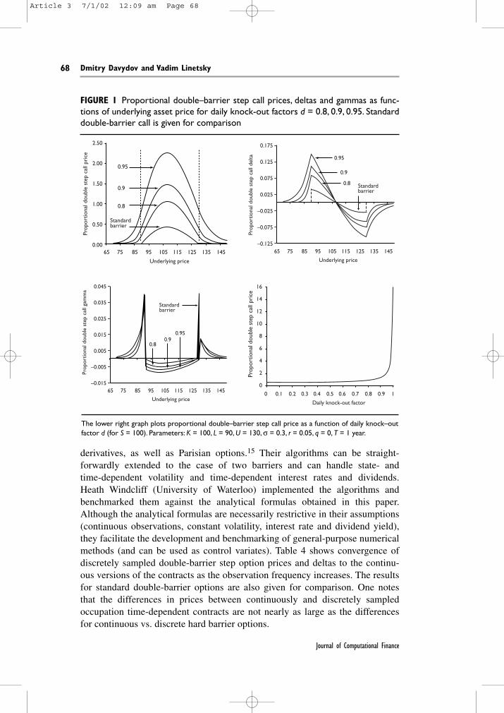
derivatives, as well as Parisian options.15 Their algorithms can be straight-forwardly extended to the case of two barriers and can handle state- andtime-dependent volatility and time-dependent interest rates and dividends.Heath Windcliff (University of Waterloo) implemented the algorithms andbenchmarked them against the analytical formulas obtained in this paper.Although the analytical formulas are necessarily restrictive in their assumptions(continuous observations, constant volatility, interest rate and dividend yield),they facilitate the development and benchmarking of general-purpose numericalmethods (and can be used as control variates). Table 4 shows convergence ofdiscretely sampled double-barrier step option prices and deltas to the continu-ous versions of the contracts as the observation frequency increases. The resultsfor standard double-barrier options are also given for comparison. One notesthat the differences in prices between continuously and discretely sampledoccupation time-dependent contracts are not nearly as large as the differencesfor continuous vs. discrete hard barrier options.
Dmitry Davydov and Vadim Linetsky
Journal of Computational Finance
68
FIGURE 1 Proportional double–barrier step call prices, deltas and gammas as func-tions of underlying asset price for daily knock-out factors d = 0.8, 0.9, 0.95. Standarddouble-barrier call is given for comparison
0.95
0.9
0.8
Standardbarrier
2.50
2.00
1.50
1.00
0.50
0.0065 75 85 95 105
Underlying price
Prop
ortio
nal d
oubl
e st
ep c
all p
rice
115 125 135 145
16
14
12
10
8
6
4
2
0
0 0.1 0.2 0.3 0.4
Daily knock-out factor
Prop
ortio
nal d
oubl
e st
ep c
all p
rice
0.5 0.6 0.7 0.8 0.9 1
0.950.9
0.8
Standardbarrier
0.045
0.035
0.025
0.015
0.005
–0.005
–0.01565 75 85 95 105
Underlying price
Prop
ortio
nal d
oubl
e st
ep c
all g
amm
a
115 125 135 145
0.95
0.9
0.8 Standardbarrier
0.175
0.125
0.075
0.025
–0.025
–0.075
–0.12565 75 85 95 105
Underlying price
Prop
ortio
nal d
oubl
e st
ep c
all d
elta
115 125 135 145
The lower right graph plots proportional double–barrier step call price as a function of daily knock–outfactor d (for S = 100). Parameters: K = 100, L = 90, U = 130, σ = 0.3, r = 0.05, q = 0, T = 1 year.
Article 3 7/1/02 12:09 am Page 68
Structuring, pricing and hedging double-barrier step options
Volume 5/Number 2, Winter 2001/02
69
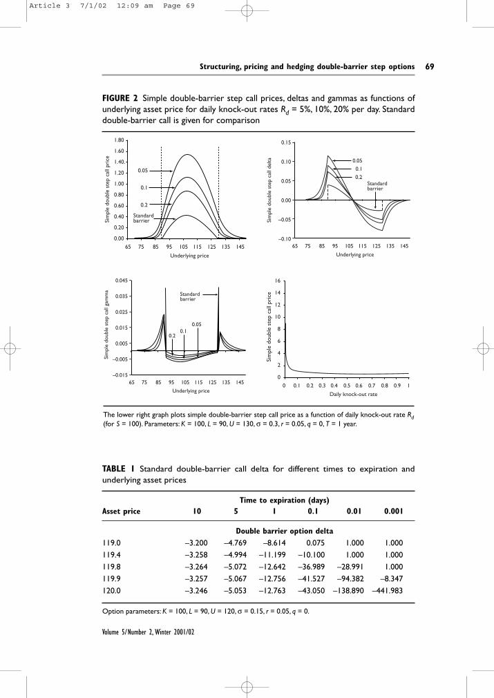
FIGURE 2 Simple double-barrier step call prices, deltas and gammas as functions ofunderlying asset price for daily knock-out rates Rd = 5%, 10%, 20% per day. Standarddouble-barrier call is given for comparison
0.05
0.1
0.2
Standardbarrier
1.80
1.60
1.40.
1.20
1.00
0.80
0.60
0.40
0.20
0.0065 75 85 95 105
Underlying price
Sim
ple
doub
le s
tep
call
pric
e
115 125 135 145
16
14
12
10
8
6
4
2
0
0 0.1 0.2 0.3 0.4
Daily knock-out rate
Sim
ple
doub
le s
tep
call
pric
e
0.5 0.6 0.7 0.8 0.9 1
0.050.1
0.2
Standardbarrier
0.045
0.035
0.025
0.015
0.005
–0.005
–0.01565 75 85 95 105
Underlying price
Sim
ple
doub
le s
tep
call
gam
ma
115 125 135 145
0.050.1
0.2Standardbarrier
0.15
0.10
0.05
0.00
–0.05
–0.1065 75 85 95 105
Underlying price
Sim
ple
doub
le s
tep
call
delta
115 125 135 145
The lower right graph plots simple double-barrier step call price as a function of daily knock-out rate Rd(for S = 100). Parameters: K = 100, L = 90, U = 130, σ = 0.3, r = 0.05, q = 0, T = 1 year.
TABLE 1 Standard double-barrier call delta for different times to expiration andunderlying asset prices
Time to expiration (days)Asset price 10 5 1 0.1 0.01 0.001
Option parameters: K = 100, L = 90, U = 120, σ = 0.15, r = 0.05, q = 0.
Article 3 7/1/02 12:09 am Page 69
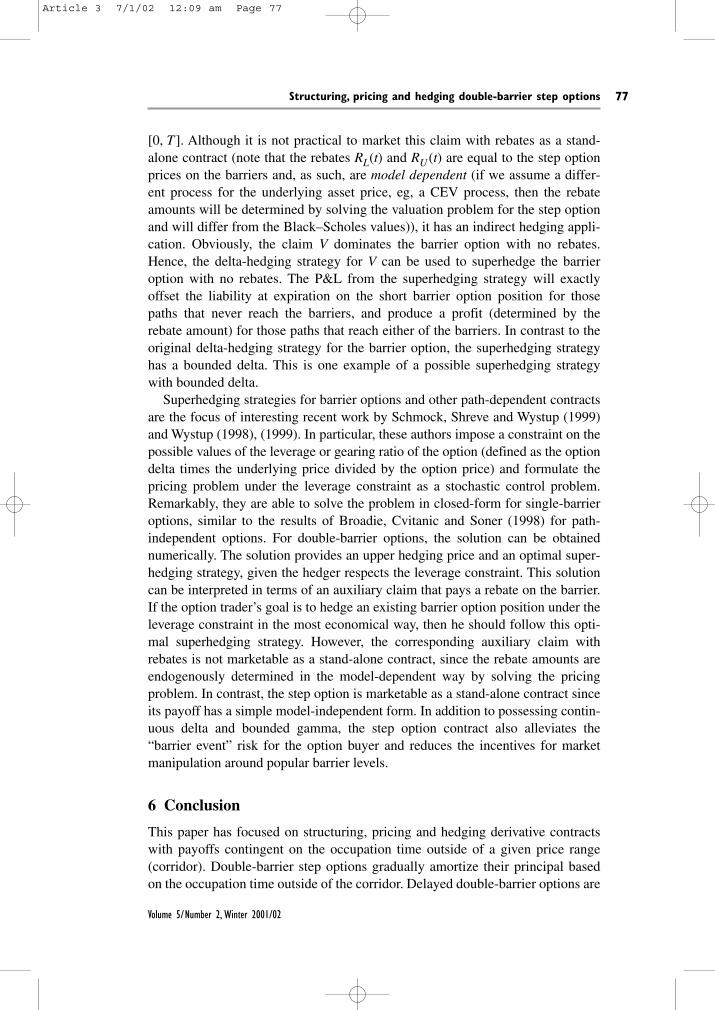
To investigate the impact of volatility smiles, the finite-difference algorithmwas extended to handle state-dependent volatility. The constant elasticity of vari-ance (CEV) model of Cox (1975) and Cox and Ross (1976) with negative elas-ticity of the local volatility function (β < 0)
provides a simple example of a process that leads to downward-sloping volati-lity (half) smiles (skews) similar to the ones observed in the S&P 500 stockindex options market. The parameter δ fixes at-the-money volatility level, whileβ controls the slope of the volatility skew. Typical implied parameter estimatesof β implicit in stock index option prices are in the –2 to –4 range (theBlack–Scholes model with flat volatility corresponds to the case β = 0). Boyleand Tian (1999) investigate the effect of the CEV elasticity β on prices ofbarrier and lookback options in the numerical trinomial lattice framework.
d d dS r q S t S Bt t t t= − + +( ) δ β1
Dmitry Davydov and Vadim Linetsky
Journal of Computational Finance
70
FIGURE 3 Delayed double-barrier step call prices, deltas and gammas as functionsof underlying asset price for knock-out windows θ = 1, 5, 10 days. Standard double-barrier call is given for comparison
10 days
5 days
1 day
Standardbarrier
1.80
1.60
1.40.
1.20
1.00
0.80
0.60
0.40
0.20
0.0065 75 85 95 105
Underlying price
Del
ayed
dou
ble
barr
ier
call
gam
ma
115 125 135 145
16
14
12
10
8
6
4
2
0
0 50 100 150 200
Knock-out window (days)
Del
ayed
dou
ble
barr
ier
call
pric
e
250
10 days
5 days1 day
Standardbarrier
0.045
0.035
0.025
0.015
0.005
–0.005
–0.01565 75 85 95 105
Underlying price
Del
ayed
dou
ble
barr
ier
call
pric
e
115 125 135 145
10 days
5 days
1 day Standardbarrier
0.15
0.10
0.05
0.00
–0.05
–0.1065 75 85 95 105
Underlying price
Del
ayed
dou
ble
barr
ier
call
pric
e115 125 135 145
The lower right graph plots delayed double-barrier step call price as a function of knock-out window θ(for S = 100). Parameters: K = 100, L = 90, U = 130, σ = 0.3, r = 0.05, q = 0, T = 1 year.
Article 3 7/1/02 12:09 am Page 70
Davydov and Linetsky (2000; 2001) derive analytical expressions for barrierand lookback option prices under the CEV process, provide comparative staticsanalysis of option prices and hedge ratios, and conduct dynamic hedging simu-lation experiments to demonstrate that extrema-dependent exotic options suchas barriers and lookbacks are extremely sensitive to the slope of the volatilityskew. Figure 4 illustrates the effect of β on prices and deltas of double-barrier
Structuring, pricing and hedging double-barrier step options
Volume 5/Number 2, Winter 2001/02
71
FIGURE 4 Discretely sampled simple double-barrier step call prices and deltasunder the CEV process as functions of the underlying asset price
70 80
Asset value
Asset value
Opt
ion
valu
eD
elta
90 100 110 120 130 140 1500
0.5
1
1.5
2
2.5
3
3.5
4
β = –3
β = –2
β = –1
β = –1/2
β = 0
70 80 90 100 110 120 130 140 150
–0.1
–0.2
0
0.1
0.2
0.3
β = –3
β = –2
β = –1
β = –1/2
β = 0
Parameters: K = 100, L = 90, U = 130, r = 0.05, q = 0, T = 1 year, daily knock-out rate Rd = 0.1 (10% perday), knock-out window 10 days.The CEV elasticity parameter β = 0, –0.5, –1, –2, –3 (β = 0 correspondsto the lognormal process). For each β, the parameter δ is selected so that the local volatility level at theasset level S = 100 is equal to 30%.The barriers are monitored once a day.
Article 3 7/1/02 12:09 am Page 71
step options. Similar to the extrema-dependent contracts, occupation time-dependent contracts are also very sensitive to the elasticity parameter β (and,hence, to the slope of the volatility skew). See Davydov and Linetsky (2001) forfurther details on the CEV process.
5 Hedging
5.1 Problems with dynamic hedging of barrier options
Consider an option hedger who sold a standard European call. Assume the stan-dard perfect markets assumptions hold and the underlying asset followsgeometric Brownian motion. Then, according to the Black and Scholes (1973)argument, the hedger should execute a dynamic delta-hedging strategy by con-tinuously trading in the underlying risky asset and the risk-free bond. The bal-ance of the hedger’s trading account will perfectly offset the liability on the shortoption position for all terminal values of the underlying price. For a standardEuropean call, the hedge ratio or delta ∆ = ∆(S, t) is a continuous function of Sand always lies inside the interval [0, 1].
The situation is more complicated for barrier options. First, the barrier optiondelta is discontinuous at the barrier for all times to maturity. For a double-barriercall, it is positive near the lower barrier and negative near the upper barrier (seeFigure 1). To hedge close to the upper barrier, the hedger needs to take a shortposition in the underlying asset. As the underlying goes up and the barrier iscrossed, the entire short hedge position has to be liquidated at once on a stop-loss order. The execution of a large stop-loss order has a risk of “slippage” (buy-ing back the underlying asset at a price greater than the barrier level). This addsto the cost of hedging barrier options and is reflected in wider bid–ask spreadsfor these OTC contracts. Moreover, in the currency markets, it sometimes hap-pens that many barrier option positions with closely placed barriers exist in themarket (“densely mined market”). Consequently, all barrier option writers placetheir stop-loss buy orders around the same barrier levels to cover their shorthedges. When the market rallies through the barrier, all stop-loss orders get trig-gered and, due to liquidity limitations, this results in a further rally (“liquidityhole”) and poor execution (“slippage”). See Taleb (1997) for a detailed discus-sion of these phenomena of “mined markets” and “liquidity holes”.
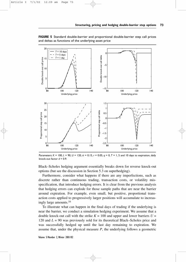
Second, a potentially more serious problem with barrier options that knock outin-the-money (reverse knock-out options), such as up-and-out calls, down-and-outputs and double-barrier options, is that their delta is unbounded as expirationapproaches and the underlying price nears the barrier. For up-and-out and double-barrier calls, delta tends to – ∞ as S → U and t → T, and the hedger is forced totake progressively larger short positions in the underlying. Figure 5 plots thedouble-barrier call delta as a function of the underlying price with 10, 5 and 1 dayremaining to expiration. Table 1 gives the values of delta for various times to expi-ration and underlying prices in this dangerous area near the barrier close toexpiration. In practice, arbitrarily large short positions are not acceptable, and the
Dmitry Davydov and Vadim Linetsky
Journal of Computational Finance
72
Article 3 7/1/02 12:09 am Page 72
Black–Scholes hedging argument essentially breaks down for reverse knock-outoptions (but see the discussion in Section 5.3 on superhedging).
Furthermore, consider what happens if there are any imperfections, such asdiscrete rather than continuous trading, transaction costs, or volatility mis-specification, that introduce hedging errors. It is clear from the previous analysisthat hedging errors can explode for those sample paths that are near the barrieraround expiration. For example, even small, but positive, proportional trans-action costs applied to progressively larger positions will accumulate to increas-ingly large amounts.16
To illustrate what can happen in the final days of trading if the underlying isnear the barrier, we conduct a simulation hedging experiment. We assume that adouble knock-out call with the strike K = 100 and upper and lower barriers U =120 and L = 90 was previously sold for its theoretical Black–Scholes price andwas successfully hedged up until the last day remaining to expiration. Weassume that, under the physical measure P, the underlying follows a geometric
Structuring, pricing and hedging double-barrier step options
Volume 5/Number 2, Winter 2001/02
73
FIGURE 5 Standard double-barrier and proportional double-barrier step call pricesand deltas as functions of the underlying asset price
80 100 120 1400
5
10
15
20
Underlying price
Dou
ble
knoc
k-ou
t ca
ll pr
ice
80 100 120 140–15
–10
–5
0
Underlying price
Dou
ble
knoc
k-ou
t ca
ll de
lta
80 100 120 1400
5
10
15
20
25
30
Underlying price
Prop
ortio
nal s
tep
call
pric
e
80 100 120 140–2.5
–2
–1.5
–1
–0.5
0
0.5
1
1.5
Underlying price
Prop
ortio
nal s
tep
call
delta
T = 10 daysT = 5 days T = 1 day
Parameters: K = 100, L = 90, U = 120, σ = 0.15, r = 0.05, q = 0, T = 1, 5 and 10 days to expiration, dailyknock-out factor d = 0.9.
Article 3 7/1/02 12:09 am Page 73
Brownian motion with the volatility σ = 15% and drift m = 12%, the risk-freerate is r = 5%, and there are no dividends (q = 0). We consider four hedging fre-quencies: 1, 10, 100 and 1,000 times per day. For each hedging frequency, twocases are considered: without transaction costs and with proportional transactioncosts of 0.1%. For each case, 10,000 sample paths are simulated. Table 2 givesthe summary statistics for dynamic hedging of the double-barrier call17 over thelast day prior to expiration when the underlying is just below the barrier at thebeginning of the period, S0 = 119. For each case, the mean, standard deviationand the 99th and 99.9th percentiles of the terminal profit and loss (P&L) distri-bution (hedging error) are reported. First, consider the case without transactioncosts. As hedging frequency increases, the hedging error converges to zeroextremely slowly. Even when hedging 1,000 times per day, the standard devia-tion is still sizable and equal to 50 cents. Moreover, the 99th and 99.9th per-centiles are very large at –$1.295 and –$4.734, respectively. Furthermore, whenproportional transaction costs are introduced, hedging errors quickly explode.
A recently introduced method of static hedging (Carr, Ellis and Gupta, 1997;Derman, Ergener and Kani, 1995; Andersen, Andreasen and Eliezer, 2000) ofbarrier options with portfolios of vanilla calls and puts is an alternative todynamic delta-hedging. Toft and Xuan (1998) study the performance of statichedging for up-and-out calls. They study static hedges proposed by Derman,Ergener and Kani (1995) that replicate an up-and-out call with a portfolio ofvanilla calls of different maturities. They find that performance of static hedges,as with dynamic hedging schemes, is extremely sensitive to the discontinuity in
Dmitry Davydov and Vadim Linetsky
Journal of Computational Finance
74
TABLE 2 Dynamic delta hedging experiment. Standard double-barrier call and pro-portional double-step call are hedged during the last day prior to expiration
Hedging frequency (times per day)1 10 100 1,000 1 10 100 1,000
Hedging frequencies: 1, 10, 100 and 1,000 times per day. The cases without transaction costs and withproportional transaction costs of 0.1% are simulated. For each case, 10,000 Monte Carlo trials are simu-lated. The mean, standard deviation, and the 99th and 99.9th percentiles (100th and 10th worstoutcomes) of the hedging error are given. Option parameters: K = 100, L = 90, U = 120, σ = 0.15, r =0.05, q = 0, d = 0.9.
Article 3 7/1/02 12:09 am Page 74
payoff on the barrier. They conclude: “In general, options with large discontinu-ous payoffs on the barrier are very difficult to delta hedge because the option’sdelta changes rapidly when the barrier is hit. It appears that a static hedge per-forms poorly in exactly the same situations as those where delta hedges are in-adequate.” Thus, reverse knock-out options with “hard” barriers are difficult tohedge not only dynamically, but statically as well.
We conclude this section with the quote from Tompkins (1997): “Therefore, itis not surprising that these products tend to trade in the Over the Counter marketat prices which are approximately double the theoretical price. Clearly, thedynamic hedging of these products is problematic at best.”
5.2 Dynamic hedging of step options
In contrast to “hard” barrier options, the step option delta is continuous for alltimes to maturity τ > 0 and remains bounded as τ → 0. Consider a proportionaldouble-barrier step call with strike K = 100, upper and lower barriers U = 120and L = 90 and daily knock-out factor d = 0.9. Figure 5 plots step option valuesand deltas with 10, 5, and 1 day remaining to expiration. The largest negativevalue of delta is attained at the upper barrier. For example, for d = 0.9 and σ =15%, the largest negative value of delta, ∆* = –2.215, is attained at the upperbarrier with τ* = 13 days remaining to expiration. Table 3 gives the largest nega-tive values of delta, ∆*, and respective times to expiration, τ*, for different val-ues of daily knock-out factor and volatility.
Since the step option delta is bounded by a reasonable value, we expect a sig-nificant improvement in performance of the delta-hedging scheme over the“hard” double-barrier option. Table 2 gives the summary statistics for a dynamichedging experiment similar to the one reported for the “hard” double-barriercall, where a step option is hedged over the last trading day before expirationwhen the initial underlying price is near the barrier, S0 = 119. The hedging errorsare orders-of-magnitude smaller than the errors for the “hard” double-barrier calland rapidly converge to zero as hedging frequency increases. The finite knock-out rate bounds the delta and essentially solves the problem of hedging in thedangerous area close to expiration and near the barrier.
Structuring, pricing and hedging double-barrier step options
Volume 5/Number 2, Winter 2001/02
75
TABLE 3 Largest negative values of delta, ∆*, and respective times to maturity, τ*,for different values of daily knock-out factor and volatility
Proportional double-step call parameters: K = 100, L = 90, U = 120, r = 0.05, q = 0.
Article 3 7/1/02 12:09 am Page 75
5.3 Interpretation in terms of rebates and superhedging
Let v(t, S), t ∈[0, T], S ∈[L, U], be the value function of a (newly-written) pro-portional double-barrier step call. Define RL(t) := v(t, L), RU (t) := v(t, U), t ∈[0, T]. Consider an auxiliary contingent claim V with the cash flows:
❑ An amount max(ST – K, 0) is paid at expiration T if the barriers were neverreached during the claim’s lifetime;
❑ A rebate RL(TL ) is paid at the first hitting time TL if the lower barrier isreached first;
❑ A rebate RU (TU) is paid at the first hitting time TU if the upper barrier isreached first.
This is a double-barrier option with time-dependent rebates equal to the values ofthe step option on the barriers.
Let V(t, S) be the value function of the claim V. Since it is equal to the stepoption value v(t, S) on the barriers, has the same terminal condition at expira-tion, and satisfies the Black–Scholes PDE for S ∈(L, U) and t ∈[0, T ), it is equalto the step option value v(t, S) everywhere in the range S ∈[L, U] for all t ∈
Dmitry Davydov and Vadim Linetsky
Journal of Computational Finance
76
TABLE 4 Convergence of discretely sampled simple double-barrier step call pricesand deltas to continuously sampled values as the observation frequency increases
Barrier monitoring frequency (times per day)Underlying 1 2 10 Continuous
Barrier monitoring frequencies: 1, 2, 10 times per day. Daily knock–out rates Rd = 5%, 10%, and 20% perday. Standard “hard” double–barrier call prices and deltas are given for comparison. Parameters: K = 100,L = 90, U = 130, σ = 0.3, r = 0.05, q = 0, T = 1 year.
Article 3 7/1/02 12:09 am Page 76
[0, T]. Although it is not practical to market this claim with rebates as a stand-alone contract (note that the rebates RL(t) and RU (t) are equal to the step optionprices on the barriers and, as such, are model dependent (if we assume a differ-ent process for the underlying asset price, eg, a CEV process, then the rebateamounts will be determined by solving the valuation problem for the step optionand will differ from the Black–Scholes values)), it has an indirect hedging appli-cation. Obviously, the claim V dominates the barrier option with no rebates.Hence, the delta-hedging strategy for V can be used to superhedge the barrieroption with no rebates. The P&L from the superhedging strategy will exactlyoffset the liability at expiration on the short barrier option position for thosepaths that never reach the barriers, and produce a profit (determined by therebate amount) for those paths that reach either of the barriers. In contrast to theoriginal delta-hedging strategy for the barrier option, the superhedging strategyhas a bounded delta. This is one example of a possible superhedging strategywith bounded delta.
Superhedging strategies for barrier options and other path-dependent contractsare the focus of interesting recent work by Schmock, Shreve and Wystup (1999)and Wystup (1998), (1999). In particular, these authors impose a constraint on thepossible values of the leverage or gearing ratio of the option (defined as the optiondelta times the underlying price divided by the option price) and formulate thepricing problem under the leverage constraint as a stochastic control problem.Remarkably, they are able to solve the problem in closed-form for single-barrieroptions, similar to the results of Broadie, Cvitanic and Soner (1998) for path-independent options. For double-barrier options, the solution can be obtainednumerically. The solution provides an upper hedging price and an optimal super-hedging strategy, given the hedger respects the leverage constraint. This solutioncan be interpreted in terms of an auxiliary claim that pays a rebate on the barrier.If the option trader’s goal is to hedge an existing barrier option position under theleverage constraint in the most economical way, then he should follow this opti-mal superhedging strategy. However, the corresponding auxiliary claim withrebates is not marketable as a stand-alone contract, since the rebate amounts areendogenously determined in the model-dependent way by solving the pricingproblem. In contrast, the step option is marketable as a stand-alone contract sinceits payoff has a simple model-independent form. In addition to possessing contin-uous delta and bounded gamma, the step option contract also alleviates the“barrier event” risk for the option buyer and reduces the incentives for marketmanipulation around popular barrier levels.
6 Conclusion
This paper has focused on structuring, pricing and hedging derivative contractswith payoffs contingent on the occupation time outside of a given price range(corridor). Double-barrier step options gradually amortize their principal basedon the occupation time outside of the corridor. Delayed double-barrier options are
Structuring, pricing and hedging double-barrier step options
Volume 5/Number 2, Winter 2001/02
77
Article 3 7/1/02 12:09 am Page 77
extinguished in their entirety as soon as the occupation time exceeds a pre-specified knock-out window.
From the option buyer’s perspective, these contracts serve as “no-regrets”alternatives to the currently traded double-barrier contracts. From the optionseller’s perspective, these contracts solve the problem of discontinuous andunbounded delta that complicates hedging of double-barrier options. Occupationtime-based contracts are easier to hedge than “hard” barrier options and, thus,smaller bid/ask spreads over the theoretical price would be required to compen-sate for the risks inherent in hedging the option sale.
Appendix A – Proofs
PROOF OF PROPOSITION 3.1 For any complex number s with Re(s) > λ2 ⁄ 2, con-sider the Laplace transform
According to the Feynman–Kac theorem (Karatzas and Shreve, 1991, Theorem4.9, p. 271), the function gρ–, ρ+(s, λ, u, k, x) is the unique continuous andcontinuously differentiable solution of the ODE
where f(x) = eλx1{x ≥ k}. The function g and its first derivative gx are continuousat the barriers 0 and u. The solution to this inhomogeneous ODE can beexpressed in the form
(51)
where Gρ–, ρ+(s; x, y) is the resolvent kernel that solves the ODE (δ(x) is theDirac’s delta function)
subject to the continuity boundary conditions at the lower barrier at zero and theupper barrier at u (the continuity boundary conditions insure that both the resol-vent and its first derivative are continuous at the barriers and, consequently, thefunction g is continuous and continuously differentiable at the barriers)
lim ( ; , ) ( ; , ), ,ε ρ ρ ρ ρε ε
→ + − + − ++ − −( ) =0
0G s u y G s u y
lim ( ; , ) ( ; , ), ,ε ρ ρ ρ ρε ε
→ + − + − +− −( ) =0
0G s y G s y
12 0G s G x yxx x x u− + +( ) = − −−
≤{ }+
≥{ }ρ ρ δ1 1 ( )
g s u k x f y G s x y y G s x y yy
kρ ρ ρ ρ
λρ ρλ− + − + − += =
−∞
∞ ∞
∫ ∫, , ,( , , , , ) ( ) ( ; , ) ( ; , )d e d
12 0g s g f xxx x x u− + +( ) = −−
≤{ }+
≥{ }ρ ρ1 1 ( )
g s u k x T u k x tsTρ ρ ρ ρλ λ− + − += −
∞
∫, ,( , , , , ) ( , , , , )e dΨ
0
Dmitry Davydov and Vadim Linetsky
Journal of Computational Finance
78
Article 3 7/1/02 12:09 am Page 78
and the asymptotic boundary conditions at infinity
In the notation of Proposition 3.1 (Equations (38)–(44)), the unique solution tothis problem is given by:
❑ Region (1,1): x ≤ 0, y ≤ 0
❑ Region (1,2): x ≤ 0, 0 ≤ y ≤ u
❑ Region (1,3): x ≤ 0, u ≤ y
❑ Region (2,2): 0 ≤ x ≤ u, 0 ≤ y ≤ u
❑ Region (2,3): 0 ≤ x ≤ u, u ≤ y
❑ Region (3,3): u ≤ x, u ≤ y
G s x yBx y u x y
ρ ργ γ
γ− + = −
− − − −,
, ( )( ; , )3 3 21e e
∆
G s x y y u x u x uρ ρ
γ β βα β α β− + = + − −[ ]− − + − −,
, ( ) ( ) ( )( ; , ) ( ) ( )2 3 2
∆e e e
G s x yx y
x y
x y x y
u x y
ρ ρ
ββ
β β
β β
β βα β β γ
α β β γ
α β β γ
− + = + + −[− − − +( )
− − + ]
− −+
− − −
− +
,, ( )
( ) ( )
( )
( ; , ) ( )( )
( )( )
( )( )
2 2
2
1ee
e e
e e
∆
G s x y x u u yρ ρ
α β γβ− + = + + −,
, ( )( ; , )1 3 4
∆e
G s x y x y u yρ ρ
α β ββ γ β γ− + = − + +[ ]−,
, ( )( ; , ) ( ) ( )1 2 22
∆e e e
G s x yAx y x y
ρ ρα α
α− + = +
− − +,
, ( )( ; , )1 1 1e e
∆
lim ( ; , ),x
G s x y→±∞
− + =ρ ρ 0
lim ( ; , ) ( ; , ), ,
ε
ρ ρ ρ ρε ε→ +
− + − +∂
∂+ −
∂
∂−
=
00
G
xs u y
G
xs u y
lim ( ; , ) ( ; , ), ,
ε
ρ ρ ρ ρε ε→ +
− + − +∂
∂−
∂
∂−
=
00
G
xs y
G
xs y
Structuring, pricing and hedging double-barrier step options
Volume 5/Number 2, Winter 2001/02
79
Article 3 7/1/02 12:09 am Page 79
The solutions in the regions (2,1) (0 ≤ x ≤ u, y ≤ 0), (3,1) (u ≤ x, y ≤ 0) and (3,2)(u ≤ x, 0 ≤ y ≤ u) are found from the symmetry of the resolvent:
As a function of y, the resolvent is a linear combination of exponentials of theform ecy. For all complex s with Re(s) > λ2⁄ 2, the integral in y on the right-handside of Equation (51) exists and can be calculated in closed form. Finally, theLaplace transform of the function Ψ̃ρ–, ρ+ is obtained by subtracting the expres-sion (26) for the Laplace transform of the function ΨDB from the expression forthe Laplace transform of the function Ψρ–, ρ+. After some tedious but straight-forward algebra the final result can be represented in the form (37). ■■
PROOF OF PROPOSITION 3.2 First, we note that for any non-negative t and positiveρ
This implies the relationship between the payoffs of delayed double-barrieroptions and proportional double-barrier step options
(52)
Then, taking present values of both sides of Equation (52) and appealing toFubini’s theorem to interchange the order of integration and expectation, wearrive at the relationship between the option prices
(53)
Finally, the first equality in Equation (49) follows from (53) by invertingthe Laplace transform. The second equality in Equation (49) follows fromEquation (47) (note that CDB is independent of ρ and thus Lθ
–1{(1 ⁄ρ)CDB} =Lθ
–1{(1 ⁄ρ)}CDB = CDB). ■■
PROOF OF PROPOSITION 3.2 First, we note that for any non-negative t and positiveρ
This implies the relationship between the payoffs of simple and proportionaldouble-barrier step options
θθ
θρ
ρθ ρe max d e− −∞
−
=∫ 1 0
12
0
t t,
e ddelayed−∞
=∫ ρθθ ρθ
ρC S T K L U C S T K L U( ; , , , ) ( ; , , , )
1
0
e d e−+ ≤
− +∞
− +
− +−( )
= −( )∫ ρθ
τ τ θρ τ τθ
ρ1
{ }( )max , max ,
L U
L US K S KT T01
00
e d e−≤
−∞
=∫ ρθθ
ρθρ
1{ }tt1
0
G s x y G s y xi j j iρ ρ ρ ρ− + − +=
,,
,,( ; , ) ( ; , )
Dmitry Davydov and Vadim Linetsky
Journal of Computational Finance
80
Article 3 7/1/02 12:09 am Page 80
(54)
Then, taking present values of both sides of Equation (54) and appealing toFubini’s theorem to interchange the order of integration and expectation, wearrive at the relationship between the option prices
(55)
Finally, the first equality in Equation (50) follows from (55) by inverting theLaplace transform and recalling that θ = 1/R. The second equality in Equation(50) follows from Equation (47) (note that CDB is independent of ρ and thusLθ
Appendix B – Inverting Laplace transforms via the Euler method
If a given function F(s) is analytic in the complex region Re(s) > c0, then theinverse Laplace transform of F(s) can be calculated as the Bromwich contourintegral
(56)
where t > 0, c > c0, and i = ��–1. The functions on the right hand side of Equation (37) are analytic in the
region Re(s) > c0 = λ2⁄ 2, and the inverse Laplace transform can be calculatednumerically using a contour of integration to the right of λ2⁄ 2. To invert Laplacetransforms numerically we use the Euler method due to Abate and Whitt (1995).This method was previously applied to option pricing problems by Fu, Madanand Wang (1997) who used it to invert the Geman and Yor (1993) Laplace trans-form to compute Asian option prices. First, letting the contour of integration be avertical line Re(s) = c such that F(s) has no singularities on or to the left of it(Re(s) > λ2⁄ 2 in our case), the Bromwich integral can be re-written in the form
The integral is evaluated numerically by means of the trapezoidal rule. If we usea step size h = π ⁄2t and let c = A ⁄2t, we obtain the nearly alternating series:
f t F si
F s s ut F c iu ut
c i
c ist
ct
( ) { ( )} ( ) cos Re[ ( )]= = = +−
− ∞
+ ∞ ∞
∫ ∫L 1
0
1
2
2
π πe d
ed
f t F si
F s st
c i
c ist( ) { ( )} ( )= =−
− ∞
+ ∞
∫L 1 1
2πe d
θ θρ
ρθρ
θe dsimple−
∞
=∫ C S T K L U C S T K L U112
0
( ; , , , ) ( ; , , , )
θθ
τ τ θ
ρ
ρθ
ρ τ τ
e max d
e
− − +∞
− +
− +( )[ ] −( )
=
−( )
∫− +
11
0 0
10
0
2
L U T
T
S K
S KL U
, max ,
max ,( )
Structuring, pricing and hedging double-barrier step options
Volume 5/Number 2, Winter 2001/02
81
Article 3 7/1/02 12:09 am Page 81
The Euler summation is used to numerically calculate the series. The functionf(t) is approximated by the weighted average of partial sums
where the partial sums are
The choice of parameters A = 2ct, n and m is dictated by the desired accuracy.The parameter A has to satisfy the condition A > 2c0t, so that the contour of inte-gration lies to the right of all the singularities of F(s). To select A in that region,a discretization error can be estimated as (see Abate and Whitt, 1995, for detailson this error estimate)
It is often straightforward to find an upper bound for f(t) in financial applica-tions. For example, the step option price Cρ–, ρ+ (S; T, K, L, U) is always lowerthan the underlying price, Cρ–, ρ+ (S; T, K, L, U) ≤ S, and ed can be estimated as
The choice of A = δ ln 10 produces a discretization error | ed | ≤ 10–δS, and, inparticular, A = 18.4 corresponds to δ = 8.
Further, parameters m and n control the truncation error associated with theEuler summation. Abate and Whitt (1995) suggest to start with m = 11 and n =15 and then adjust n as needed. We found that n as small as 5 gives satisfactoryresults in our application.
To implement the pricing formulas (49) and (50), we need to invert doubleLaplace transforms numerically. For a function F(s1, s2) analytic in the complexdomain where Re(s1) ≥ c1 and Re(s2) ≥ c2, the inverse double Laplace trans-form can be represented as a bi-variate Bromwich integral
(57)
where t1, t2 > 0.
f t t F s si
F s s s st ts t s t
c i
c i
c i
c i
( , ) ( , )( )
( , )1 21 1
1 2 2 1 2 2 11 21 1 2 2
2
2
1
11
2= { }{ } =− − +
− ∞
+ ∞
− ∞
+ ∞
∫∫L Lπ
e d d
e Sd
A
A≤−
−
−e
e1
e f k tdk A
k
= +( )−
=
∞
∑e ( )2 11
s tt
FA
t tF
A j i
tn k
A Aj
j
n k
+=
+
=
+ − +
∑( ) ( ) Re
e e2 2
12 2
12
2
π
f t F sm
ks tt
mn k
k
m
( ) { ( )} ( )= ≈
− −+
=∑L 1
0
2
f tt
FA
t tF
A j i
t
A Aj
j
( ) ( ) Re≈
+ − +
=
∞
∑e e2 2
12 2
12
2
π
Dmitry Davydov and Vadim Linetsky
Journal of Computational Finance
82
Article 3 7/1/02 12:09 am Page 82
When ρ– = ρ+ = ρ, the functions on the right-hand side of Equation (37) con-sidered as functions of two complex variables s and ρ are analytic in the regionwhere Re(s) > λ2⁄ 2 and Re(ρ) > 0.
The Euler algorithm for numerical inversion of Laplace transforms wasextended to multiple dimensions by Choudhury, Lucantoni and Whitt (1994).First, the bi-variate Bromwich integral (57) is discretized similar to the one-dimensional case:
Then, to calculate the nearly alternating series, the Euler summation is used (weset l1 = l2 = 1 in the general algorithm of Choudhury, Lucantoni and Whitt(1994) as this choice is enough to achieve the desired accuracy in ourapplication):
where
The parameters A1, A2, n and m control computation accuracy.The discretization error is controlled by A1 and A2. The truncation error is
controlled by m and n. Choudhury, Lucantoni and Whitt (1994) suggest thechoice of A1 = A2 = 19.1, m = 11 and n = 38. As in the one-dimensional case, ncan be adjusted as needed. We found that the choice of m = 11 and n = 10 pro-duces satisfactory results for our application.
Φkm q
q
n p
p
m m
p
FA q i
t
A k i
tF
A k i
t
A q i
t
= −
×
− −
+− −
−
=
+
=∑∑2 1
2
2
2
2
2
2
2
2
00
1
1
2
2
1
1
2
2
( )
, ,π π π π
sn Kk
kk
n K
+=
+
= −∑ ( ) Re[ ]11
Φ
f t tt t
FA
t
A
t
m
Ks
A Am
K
m
n K( , ) ,( )
1 2
2
1 2
1
1
2
2 0
1 2
2
1
2 2 22≈
+
+−
=+∑e
f t tt t
FA
t
A
t
FA j i
t
A k i
t
FA
A A
k
k
j
j
( , ) ,
( ) Re ( ) ,
( )
1 2
2
1 2
1
1
2
2
1
1
1
2
20
1
1 2
2
1
2 2 2
1 12
2
2
2
≈
+ − −− −
+−
+
=
∞
=
∞
∑ ∑
e
π π
22
2
2
21
2
2
k i
t
A j i
t
π π,
−
Structuring, pricing and hedging double-barrier step options
Volume 5/Number 2, Winter 2001/02
83
Article 3 7/1/02 12:09 am Page 83
1. In addition to their popularity over-the-counter, several types of barrier options are tradedon securities exchanges. Examples of exchange-traded barrier options are single- and dou-ble-barrier knock-out call and put warrants on the Australian stock index, the AllOrdinaries Index, introduced in 1998 by the Australian Stock Exchange (ASE). Thesewarrants are Parisian-style. They knock out after the underlying index stays beyond thebarrier for three consecutive days. We thank Glen Kentwell for bringing these warrants toour attention.
2. Delayed barrier options knock in or out as soon as the occupation time beyond the barrierlevel exceeds a pre-specified knock-in or knock-out window (e.g., ten trading days). Thesecontracts are also called cumulative Parisian options by Chesney, Jeanblanc-Pique andYor (1997). Delayed barrier options and step options have different properties. The formerknock in or out in their entirety as soon as the occupation time exceeds the knock-in orknock-out window, while the latter knock in or out gradually in time. Other interestingalternative barrier option contract designs proposed in the literature include Parisianoptions of Chesney, Jeanblanc-Picque and Yor (1997) and Chesney et al. (1997) and softbarrier options of Hart and Ross (1994).
3. See Huggonier (1999) and Pechtl (1995) for more examples of occupation time-dependentcontracts. See Akahori (1995), Dassios (1995) and Miura (1992) for a related class ofpath-dependent quantile options.
4. For details on the Feynman-Kac method and its applications to calculations of variousBrownian functionals see Borodin and Salminen (1996), Fitzsimmons and Pitman (1998),Jeanblanc-Picque, Pitman and Yor (1997), Karatzas and Shreve (1991), and Revuz and Yor(1999).
5. Fu, Madan and Wang (1997) apply the Euler algorithm to compute the Geman-Yor Asianoption formula.
6. All options in this paper are European style. In the interest of brevity only call options arediscussed. Puts are treated similarly.
7. We assume that the strike is inside the range (L, U) for all options in this paper(L < K < U).
8. In the present context of continuous monitoring, nL– and nU
+ do not have to be integers.They represent occupation times measured in days, rather than years. In Section 4.2 wediscuss discretely (daily) monitored occupation time contracts where nL
– and U+ become
integers.
9. Note that if we naively define the payoff as (1 – R(τL– + τU
+)) max (ST – K, 0), it couldbecome negative for sufficiently large times outside of the range.
10. After this paper was completed we received preprints Fusai (1999) and Fusai and Tagliani(2001). They focus on pricing a corridor option with the payoff (τ (L, U) – K)+ based onthe law of the occupation time of a corridor. The problem in this paper is more generalsince our payoffs depend both on the occupation times and the terminal asset price, andthe pricing relies on their joint law.
11. Note that the days do not have to be consecutive. This is in contrast with Parisian optionsthat require n consecutive days beyond the barrier to knock out.
12. For our purposes it is more convenient to work with the Brownian motion Wt starting at xand use representation (15), rather than with the standard Brownian motion Bt starting atthe origin and the conventional representation St = Seσ(Bt + νt).
13. Note that all of the quantities α, … , D are functions of the transform variable s,
Dmitry Davydov and Vadim Linetsky
Journal of Computational Finance
84
Article 3 7/1/02 12:09 am Page 84
α = α(s), … , D = D(s). To lighten notation we do not show this dependence explicitly.
14. We are grateful to Peter Forsyth, Ken Vetzal and Heath Windcliff for independently veri-fying some of our computational results via numerical finite-difference schemes.
15. Discretely monitored occupation time options are also studied by Fusai and Tagliani(2001).
16. A similar situation with European digital options is documented by Gallus (1997).
17. It is assumed that if the barrier is crossed, the hedge is liquidated at the price equal to thebarrier (no slippage).
REFERENCES
Abate, J., and Whitt, W. (1995). Numerical inversion of Laplace transforms of probability dis-tributions. ORSA Journal of Computing, 7, 36–43.
Akahori, J. (1995). Some formulae for a new type of path-dependent option. Annals ofApplied Probability, 5, 383–8.
Andersen, L., Andreasen, J., and Eliezer, D. (2000). Static replication of barrier options: somegeneral results. Working paper, General Re Financial Products.
Black, F., and Scholes, M. (1973). The pricing of options and corporate liabilities. Journal ofPolitical Economy, 81, 637–59.
Borodin, A. N., and Salminen, P. (1996). Handbook of Brownian Motion. Birkhauser, Boston.
Boyle, P. P., and Tian, Y. (1999). Pricing lookback and barrier options under the CEV process.Journal of Financial and Quantitative Analysis, 34 (Correction: P. P. Boyle, Y. Tian, andJ. Imai, Lookback options under the CEV process: a correction, JFQA web sitehttp://depts.washington.edu/jfqa/ in “Notes, Comments, and Corrections”).
Broadie, M., Cvitanic, J., and Soner, H. M. (1998). Optimal replication of contingent claimsunder portfolio constraints. Review of Financial Studies, 11, 59–79.
Broadie, M., Glasserman, P., and Kou, S. (1997). A continuity correction for discrete barrieroptions. Mathematical Finance, 7, 325–49.
Carr, P., Ellis, K. and Gupta, V. (1998). Static hedging of exotic options. Journal of Finance,53, 1165–90.
Chesney, M., Jeanblanc-Picque, M., and Yor, M. (1997). Brownian excursions and Parisianbarrier options. Annals of Applied Probability, 29, 165–84.
Chesney, M., Cornwall, J., Jeanblanc-Picque, M., Kentwell, G., and Yor, M. (1997). Parisianpricing, RISK, January, 77–9.
Cheuk, T. H. F., and Vorst, T. C. F. (1996). Complex barrier options. Journal of Derivatives, 4(Fall), 8–22.
Choudhury, G., Lucantoni, D., and Whitt, W. (1994). Multidimensional transform inversionwith applications to the transient M/G/1 queue. Annals of Applied Probability, 4, 719–40.
Cox, J. (1975). Notes on Option Pricing I: Constant Elasticity of Variance Diffusions.Working Paper, Stanford University (reprinted in Journal of Portfolio Management, 1996,22, 15–17).
Cox, D. R., and Miller, H. D. (1965). The Theory of Stochastic Processes. Wiley, New York.
Cox, J., and Ross, S. (1976). The valuation of options for alternative stochastic processes.
Structuring, pricing and hedging double-barrier step options
Volume 5/Number 2, Winter 2001/02
85
Article 3 7/1/02 12:09 am Page 85
Journal of Financial Economics, 3, 145–66.
Dassios, A. (1995). The distribution of the quantile of a Brownian motion with drift and thepricing of path-dependent options. Annals of Applied Probability, 5, 389–98.
Davydov, D., and Linetsky, V. (2000). Pricing options on scalar diffusions: an Eigenfunctionexpansion approach. Submitted for publication.
Davydov, D., and Linetsky, V. (2001). Pricing and Hedging Path-Dependent Options under theCEV Process. Management Science, 47, 949–65.
Derman, E., Ergener, D., and Kani, I. (1995). Static options replication. Journal of Deriva-tives, 2(4), 78–95.
Derman, E., and Kani, I. (1996). The ins and outs of barrier options. Derivatives Quarterly,Winter, 55–67 (Part I) and Spring, 73–80 (Part II).
Douady, R. (1998). Closed-form formulas for exotic options and their lifetime distribution.International Journal of Theoretical and Applied Finance, 2, 17–42.
Duffie, D. (1996). Dynamic Asset Pricing, 2nd Edition, Princeton University Press, Princeton,New Jersey.
Feller, W. (1971). Introduction to Probability Theory and Its Applications, Vol. II. Wiley, NewYork.
Fitzsimmons, P. J., and Pitman, J. (1997). Kac’s moment formula and the Feynman–Kac for-mula for additive functionals of a Markov process. Working paper, Berkeley.
Fu, M., Madan D., and Wang, T. (1997). Pricing Asian options: a comparison of analytical andMonte Carlo methods. Computational Finance, 2, 49–74.
Fusai, G. (1999). Corridor options and arc–sine law. Preprint, University of Florence.
Fusai, G. and Tagliani, A. (2001). Pricing of occupation-time derivatives: continuous and dis-crete monitoring. Journal of Computational Finance, 5(1), 1–37.
Gallus, C. (1999). Exploding hedging errors for digital options. Finance and Stochastics, 3,187–201.
Geman, H., and Eydeland, A. (1995). Domino effect: inverting the Laplace transform. RISK,April, 65–7.
Geman, H., and Yor, M. (1993). Bessel processes, Asian options and perpetuities.Mathematical Finance, 3, 349–75.
Geman, H., and Yor, M. (1996). Pricing and hedging double barrier options: a probabilisticapproach. Mathematical Finance, 6, 365–78.
Hart, I., and Ross, M. (1994). Striking continuity. RISK, June, 51.
He, H., Keirstead, W., and Rebholz, J. (1998). Double lookbacks. Mathematical Finance, 8,201–28.
Hsu, H. (1997). Surprised parties. RISK, April.
Hui, H. C. (1997). Time-dependent barrier option values. The Journal of Futures Markets, 17,667–88,
Hui, H. C. Lo, C. F., and Yuen, P. H. (1997). Comment on “pricing double-barrier optionsusing Laplace transforms”, Finance and Stochastics, 4, 105–7.
Hugonnier, J.-N. (1999). The Feynman–Kac formula and pricing occupation time derivatives.International Journal of Theoretical and Applied Finance, 2, 153–78.
Dmitry Davydov and Vadim Linetsky
Journal of Computational Finance
86
Article 3 7/1/02 12:09 am Page 86
Jamshidian, F. (1997). A note on analytical valuation of double barrier options. WorkingPaper, Sakura Global Capital.
Jeanblanc-Picque, M., Pitman, J., and Yor, M. (1997). The Feynman–Kac formula and decom-position of Brownian paths. Computational and Applied Mathematics, 16, 27–52.
Karatzas, I., and Shreve, S. (1991). Brownian Motion and Stochastic Calculus, 2nd Edition.Springer-Verlag, New York.
Kunitomo, N., and Ikeda, M. (1992). Pricing options with curved boundaries. MathematicalFinance, 4, 275–98.
Linetsky, V. (1998). Steps to the barrier. RISK, April, 62–5.
Linetsky, V. (1999). Step options. Mathematical Finance, 9, 55–96.
Merton, R. C. (1973). Theory of rational options pricing. Bell Journal of Economics andManagement Science, 2, 275–98.
Miura, R. (1992). A note on look-back options based on order statistics. Hitotsubashi Journalof Commerce Management, 27, 15–28.
Pechtl, A. (1995). Classified information. RISK, June, 59–61.
Pelsser, A. (2000). Pricing double barrier options using analytical inversion of Laplace trans-forms. Finance and Stochastics, 4, 95–104.
Revuz, D., and Yor, M. (1999). Continuous Martingales and Brownian Motion, Third edition,Springer, Berlin.
Rogers, L. C. G., and Zane, O. (1995). Valuing moving barrier options. ComputationalFinance, 1, 5–12.
Rubinstein, M., and Reiner, E. (1991). Breaking down the barriers. RISK, September, 28–35.
Schroder, M. (2000). On the valuation of double-barrier options: computational aspects.Journal of Computational Finance, 3 (4).
Schmock, U., Shreve, S., and Wystup, U. (1999). Valuation of exotic options under short-sell-ing constraints. Working paper, Carnegie Mellon University.
Sidenius, J. (1998). Double barrier options: valuation by path counting. ComputationalFinance, 1, 63–79.
Snyder, G. L. (1969). Alternative forms of options. Financial Analysts Journal, 25, 93–9.
Taleb, N. (1997). Dynamic Hedging. J. Wiley & Sons, New York.
Toft, K., and Xuan, C. (1998). How well can barrier options be hedged by a static portfolio ofstandard options? Journal of Financial Engineering, 7, 147–75.
Tompkins, R. (1997). Static versus dynamic hedging of exotic options: an evaluation of hedgeperformance via simulation. Net Exposure, 2, November, 1–37.
Vetzal, K., and Forsyth, P. (1999). Discrete Parisian and delayed barrier options: a generalnumerical approach. Advances in Futures and Options Research, 10, 1–15.
Wystup, U. (1998). Valuation of exotic options under short-selling constraints as a singularstochastic control problem. PhD dissertation, Carnegie Mellon University.
Wystup, U. (1999). Dealing with dangerous digitals. Working paper, http: //www.mathfinance.de
Zhang, P. (1997). Exotic Options. World Scientific, Singapore.
Structuring, pricing and hedging double-barrier step options