Bachelor’s Thesis

Studien von Top-Quark-Paaren in√s=8 TeV Daten mit dem

ATLAS-Experiment

Studies of top-quark pairs in√

s=8 TeVdata collected with the ATLAS experiment

prepared by

Jens Oltmannsfrom Norden

at the II. Physikalisches Institut

Thesis number: II.Physik-UniGö-BSc-2014/06

Thesis period: 14th April 2014 until 18th July 2014

First referee: Prof. Dr. Arnulf Quadt

Second referee: Prof. Dr. Ariane Frey

AbstractThe signature of a decay process is not unique. Instead, there are other processes withthe same signature. These processes are called background processes. Control plots aremade to estimate the fraction of the background processes in the given data. PlotFactoryis a programme used to produce such plots. This thesis is about the modifications imple-mented in the PlotFactory.The modifications are renewing the HTML page produced by thy PlotFactory to makethe page clearer and to make the navigation between different sites easier. Pseudo top dis-tributions are added to the analysis. Those are used for a measurement of the top quarkdecay width. Also plots with logarithmic axis are included and goodness-of-fit tests areapplied.

ZusammenfassungDie Signatur eines Zerfallsprozesses ist nicht einzigartig, sondern es gibt andere Prozesse,deren Signatur dieselbe ist. Diese Prozesse werden Untergrundprozesse genannt. Um eineAbschätzung des Anteils der Untergrundprozesse an den gemessenen Daten zu haben,werden Controlplots gemacht. Ein Programm, das Controlplots erstellt, ist PlotFactory.In dieser Bachelorarbeit geht es um die Modifikationen, die während des Bachelorprojektsan der PlotFactory vorgenommen wurden.Die Modifikationen waren die vom Programm ausgegebene HTML Seite zu überarbeiten,um diese übersichtlicher zu machen und die Navigation zwischen verschiedenen Seiten zuerleichtern. Ebenfalls wurde eine Analyse von Pseudo Top-Quarks hinzugefügt, welche fürdie Messung der Zerfallsbreite des Top-Quarks benötigt werden. Des weiteren wurden dieControlplots durch weitere Plots mit logarithmischer Achse erweitert und Goodness-of-FitTests in den Plots ergänzt, um die Übereinstimmung von aufgenommen und generiertenDaten zu bewerten.

iii

Contents

1 Introduction 1

2 Theoretical Fundamentals 32.1 Standard Model of Particle Physics . . . . . . . . . . . . . . . . . . . . . . 3

2.1.1 Leptons and Quarks . . . . . . . . . . . . . . . . . . . . . . . . . . 32.1.2 Bosons and Interactions . . . . . . . . . . . . . . . . . . . . . . . . 42.1.3 Higgs Mechanism . . . . . . . . . . . . . . . . . . . . . . . . . . . . 6

2.2 Top Quark . . . . . . . . . . . . . . . . . . . . . . . . . . . . . . . . . . . . 62.2.1 Top Quark Properties . . . . . . . . . . . . . . . . . . . . . . . . . 62.2.2 Top Quark Production . . . . . . . . . . . . . . . . . . . . . . . . . 72.2.3 Top Quark Decay . . . . . . . . . . . . . . . . . . . . . . . . . . . . 9

3 Experimental Setup 133.1 Large Hadron Collider . . . . . . . . . . . . . . . . . . . . . . . . . . . . . 133.2 The Atlas Detector . . . . . . . . . . . . . . . . . . . . . . . . . . . . . . 14

3.2.1 Inner Detector . . . . . . . . . . . . . . . . . . . . . . . . . . . . . . 143.2.2 Calorimeter System . . . . . . . . . . . . . . . . . . . . . . . . . . . 153.2.3 Muon Spectrometer . . . . . . . . . . . . . . . . . . . . . . . . . . . 153.2.4 Trigger System . . . . . . . . . . . . . . . . . . . . . . . . . . . . . 16

4 Fundamentals of the Analysis 174.1 Background Processes . . . . . . . . . . . . . . . . . . . . . . . . . . . . . 174.2 Simulated Events and Data Samples . . . . . . . . . . . . . . . . . . . . . 184.3 b-Tagging . . . . . . . . . . . . . . . . . . . . . . . . . . . . . . . . . . . . 194.4 D3PD . . . . . . . . . . . . . . . . . . . . . . . . . . . . . . . . . . . . . . 194.5 Kinematic Quantities . . . . . . . . . . . . . . . . . . . . . . . . . . . . . . 20

5 TopRootCore 235.1 The Software Package TopRootCore . . . . . . . . . . . . . . . . . . . . . 235.2 PlotFactory . . . . . . . . . . . . . . . . . . . . . . . . . . . . . . . . . . . 23

v

Contents

6 Results 256.1 HTML Page . . . . . . . . . . . . . . . . . . . . . . . . . . . . . . . . . . . 276.2 Pseudo Top Distributions . . . . . . . . . . . . . . . . . . . . . . . . . . . 286.3 Goodness-of-Fit Test . . . . . . . . . . . . . . . . . . . . . . . . . . . . . . 30

6.3.1 χ2 Test . . . . . . . . . . . . . . . . . . . . . . . . . . . . . . . . . . 316.3.2 Kolmogorow-Smirnow Test . . . . . . . . . . . . . . . . . . . . . . . 32

6.4 Logarithmic Scale Plots . . . . . . . . . . . . . . . . . . . . . . . . . . . . 326.5 Modifications of the Layout . . . . . . . . . . . . . . . . . . . . . . . . . . 33

7 Conclusion 35

A Additional Plots 37

vi

1 Introduction

Particle physicists search for the fundamental components of matter and how they inter-act with each other. Within the last century, many elementary particles could be foundand described by the Standard Model of Particle Physics, which is the theoretical foun-dation of particle physics. This theory was tested in many different experiments, mostof them based on particle accelerators. In those machines, particles are accelerated tohigh energies and afterwards collided. Therefore particle physics is often also called HighEnergy Physics. To observe smaller structures and find heavier particles, colliders withlarger energies are needed.

At present, the collider with the highest energy is the Large Hadron Collider (LHC)at CERN in Geneva, which is designed for a beam energy of 7 TeV and a centre-of-massenergy of 14 TeV. At this energies, it is possible to search for particles which are notincluded in the Standard Model, like supersymmetric particles.

One particle in the Standard Model is the top quark, which has some unique quanti-ties making it very interesting for particle physics. The top quark is the heaviest particlein the Standard Model. Its mass is of the order of heavy atoms like gold and its lifetime isvery short, of the order of 10−25 s. The high mass makes the top quark a good candidateto find physics which is not explained in the Standard Model.A lot of top quarks are produced at the Large Hadron Collider, most of them in tt events,with the top (t) and the antitop (t), and less frequently as single tops. The top quarkdecays in different decay channels, each with a specific signature. This signature is notunique, but there are different other processes having the same signature, which are calledbackground processes. To estimate the influence of these processes on the results, con-trol plots are made. There are different programmes to create these plots, one of themis PlotFactory, a package implemented in TopRootCore. The main part of the bachelorproject was to modify this programme in order to have a better overview of the resultsand to add new analysis steps.

1

1 Introduction

The following Chapter 2 will give a short introduction to the Standard Model and alsoan overview of top quark physics. In Chapter 3, the experimental setup will be discussed.The fundamentals needed for the analysis will be explained in Chapter 4. A short intro-duction into TopRootCore and the PlotFactory will be given in Chapter 5. In Chapter 6,the results of the bachelor project are presented, followed by a conclusion in Chapter 7.In this thesis natural units with c = ~ = 1 are used.

2

2 Theoretical Fundamentals

2.1 Standard Model of Particle Physics

The Standard Model of Particle Physics, often shortened as SM, is a theory to explainparticles and there interaction on the smallest level. It was emerged from 1960 to 1970.The interactions explained by the SM are the strong interaction, the weak interactionand the electromagnetic interaction. Not included in the SM is the interaction caused bygravity, which is negligible at the today observable energy scales.The described particles are arranged into fermions and bosons, while fermions are sortedinto leptons and quarks. The bosons are mediating the forces between the particles andare called mediators.Nowadays effects are known which can not be explained by the SM, for example finitemasses of neutrinos or the existence of dark matter in the universe.

2.1.1 Leptons and Quarks

In this section the aforementioned fermions will be discussed in more detail. As introducedabove, the fermions are sorted in two substructures, the quarks and the leptons.The six different leptons and quarks are grouped into three generations, which differ inthe masses of the particles. The first generation is the lightest generation and the thirdgeneration the heaviest. All fermions are spin-1/2-particles.The leptons are sorted by isospin I3, electron number Le, muon number Lµ and taunumber Lτ in the following way:νe

e

,

νµ

µ

,

ντ

τ

. (2.1)

When including the handedness, the left-handed leptons and lepton-neutrinos form dou-blets, while the right-handed leptons form singlets and right-handed neutrinos do notexist. The lepton e is called electron, the µ muon and the τ tau lepton. These threeleptons have a charge of −e, where e denotes the elementary charge. The νe, νµ and ντ

3

2 Theoretical Fundamentals

are the corresponding neutrinos to the charged leptons. These particles are electricallyneutral, as their name indicates.The quarks are organised similar to the leptons by their isospin I3, upness U , downnessD, strangeness S, charmness C, bottomness B and topness T in the following way:u

d

,

c

s

,

t

b

. (2.2)

The Up-type quarks u, c, t are called Up, Charm, and Top quark. These quarks carry anelectric charge of +2/3e. The Down-type quarks d, s, b are called Down, Strange, Bottomquark and carry an electric charge of −1/3e. Unlike the leptons, quarks carry in additionto the electrical charge another charge, called colour charge. There are three differentpossibilities for the colour charge red, blue and green.Other quantities next to charge and mass of fermions are the third component of the weakisospin I3 and the weak hypercharge YW , which is given by YW = 2(Q− I3). The particlesare arranged that way that the particles with I3 = 1/2 are at the top of the doublet andthe particles with I3 = −1/2 are the bottom.For every fermion there is an antiparticle. The antiparticle has the same mass as thecorresponding particle but a different charge and the opposite quantum numbers, likethe isospin. Neutrinos and antineutrinos, which both do not have charge, differ in theirisospin and their handedness. Neutrinos are always left-handed, while antineutrinos arealways right-handed. Antiquarks also carry an anticolour.Quarks and antiquarks can not be observed as free particles. They always combine toform bound states or they decay. There are two possibilities for quarks and antiquarks tocombine. The first is the combination into mesons, which consist of one quark and oneantiquark. The other possibility are baryons or antibaryons which consist of three quarksor antiquarks. The process of building bound states is called hadronisation. There is onequark that exists as an almost free particle, the top quark, which decays before it is ableto hadronise into a bound state. More about the top quark will be explained in latersections. The mass and charges of all fermions are listed in Table 2.1.

2.1.2 Bosons and Interactions

The bosons are the mediators of the interactions while each interaction has its own typeof mediator. The mediator of the electromagnetic interaction is the photon, which isa spin-1-particle without a mass and without electric charge or colour charge. Photonscouple to electric charge, so just charged particles take part in the electromagnetic in-

4

2.1 Standard Model of Particle Physics

Lepton Mass [MeV] Charge [e] Quark Mass [MeV] Charge [e]e 0.510998928±11 -1 u 2.3+0.7

−0.5 2/3µ 105.6583715±35 -1 d 4.8+0.7

−0.3 −1/3τ 1776.82±0.16 -1 c 1275±25 2/3νe >2·10−6 0 s 95±5 −1/3νµ >2·10−6 0 t 173500±600 ± 800 2/3ντ >2·10−6 0 b 4180±30 −1/3

Table 2.1: Masses and charges of the different fermions [1].

teraction. Since photons are electrically neutral, γ − γ-couplings are not possible. Theelectromagnetic interaction is described by quantum electrodynamics.The mediators of the strong interaction are eight gluons which have neither mass norcharge, but carry colour charge and anticolour charge in which they differ. Gluons coupleto colour, so only quarks and hadrons take part in the strong interaction. The fact thatgluons carry a colour and anticolour themselves makes g − g−couplings possible. Thequantum field theory describing the strong interaction is quantum chromodynamics.The weak interaction can be categorised into charged weak interaction and the neutralweak interaction. The mediators of the charged weak interaction are the W + and W −

bosons. They carry a charge of ±1e and also have a finite mass of about 80.385±0.15 GeV[1], but do not carry colour charge.The mediator of the neutral weak interaction is the Z0 boson. It is not carrying a chargeor colour but has, like the W ± bosons, a non-zero mass of about 91.1876 ± 0.0021 GeV[1]. This weak interaction is described by quantum flavourdynamics.In contrast to the other interactions, the charged weak interaction is not flavour conserv-ing, so the charged weak interaction can mix between the generations of the quarks. Thismixing is possible because the eigenstates of the weak interaction are not the same as themass eigenstates. The connections between the weak eigenstates |d′⟩ , |s′⟩ , |b′⟩ and themass eigenstates |d⟩ , |s⟩ , |b⟩ are given by the CKM matrix in the following way [2]:

|d′⟩|s′⟩|b′⟩

=

Vud Vus Vub

Vcd Vcs Vcb

Vtd Vts Vtb

|d⟩|s⟩|b⟩

. (2.3)

This matrix was established by Kobayashi and Maskawa and is an expansion of theCabibbo matrix, which is the quark mixing matrix for two generations [3]. The matrixconsist of 18 parameters, while 14 are fixed by unitary conditions and choice of phase,what leads to four free parameters, three real angles and one complex phase. This phaseis responsible for CP (charge parity) violation.

5

2 Theoretical Fundamentals

The electromagnetic and the weak interactions are unified in the electroweak interactionproposed by Glashow, Salam and Weinberg [4–6].

2.1.3 Higgs Mechanism

The effort to formulate the interactions in local gauge theories failed because of the non-zero mass of the mediators in the weak interaction. One solution to this problem is theHiggs-mechanism postulated by Peter Higgs and others in 1964 [7–9]. This theory containsin addition to the three masses of the W ± and Z0 another degree of freedom. This is themass of another particle, the Higgs-boson, which is a spin-0-particle. The search of thisparticle took physicists a lot of time, but it was discovered 2012 at the Atlas and Cmscolliders at the Large Hadron Collider at CERN [10, 11]. The discovery was followed bya Nobel prize for Peter Higgs and François Englert in 2012.

2.2 Top Quark

The top quark is a particle in the SM and was discovered in 1995 at the pp colliderTevatron by the experiments CDF and DØ [12, 13]. The production mechanism was tt

production. Another possible channel is the single top production, which was observed2009 at the CDF and DØ experiments [14, 15].

2.2.1 Top Quark Properties

The top quark is the weak isospin partner of the bottom quark. This means that its spinis assumed to be 1/2 and its electrical charge is assumed to be +2/3e, but these quantitieshave not been measured yet. For the charge of the top quark the value of −4/3e has beenexcluded by several experiments, one of them the Atlas experiment [16].What makes the top quark unique and interesting is its heavy mass and its short lifetime.The mass of the top quark is measured by experiments at Tevatron and Lhc. Thecombined measurement of the four experiments Atlas, CDF, Cms and DØ had theresults in an estimated top quark mass of [17]:

173 ± 0.27(stat) ± 0.73(syst) GeV. (2.4)

This mass, which is comparable with the mass of atoms like gold, is larger than the massof the W ± boson, what gives the possibility for the top quark to decay into a real W ±

boson. Other fermions can not decay into a real W ± boson because their masses are much

6

2.2 Top Quark

lower than the one of the W ±.The most likely decay of the top quark is the decay t → Wq, while q can be an arbitrarydown-type quark, so d, s or b. This is a weak process and the probability which down-typequark is depending on the matrix element in the CKM matrix |Vtq|2. Since the matrixelement Vtb ≈ 1 [1], the top quark almost always decays in the way t → Wb and thelifetime of the top quark is extremely short, just [18]

τt ≈ 5 · 10−25 s. (2.5)

This is even shorter than the time quarks need to build bound states. This propertymakes the top quark the only quark being observed in “bare” form. Because the lifetimeis hard to measure, it is more likely to measure the decay width of the top quark andthen calculate the lifetime via

τ = ~Γ

. (2.6)

2.2.2 Top Quark Production

Top quarks are produced either in tt pairs or as single tops, while the pair-productionhas a larger cross section. The different production mechanisms with the different decaychannels will be shown in the next paragraphs.

tt Production The top-antitop pair production is the dominant production processin hadron colliders like Tevatron or Lhc. The production takes place by either qq

annihilation via qq → tt or gg fusion via gg → tt. In hadron colliders, the partons insidethe hadron are the particles taking part in the interaction, not the hadron itself. Theseprocesses are mediated by the strong interaction, so by exchange of a gluon. The leadingorder Feynman diagrams are shown in Figure 2.1.

Figure 2.1: Leading order Feynman diagrams for top antitop pair production via qqannihilation and gg fusion.

The partons inside the proton or antiproton carry only a fraction of the momentum the

7

2 Theoretical Fundamentals

hadrons carry themselves. The fraction of the momentum the partons carry is describedby the so-called Bjorken-x. The effective centre-of-mass energy s in a collision is given by

s = x1x2s, (2.7)

with xi being the momentum fraction carried by the parton i and s the square of thecentre-of-mass energy. To produce a top-antitop pair this effective centre-of-mass energyneeds to be larger than two times the mass of the top quark, so

√s ≥ 2mt. This leads to

the smallest possible Bjorken-x with a given centre-of-mass energy. If assumed that thefractions of both partons are equal, so x1 = x2, and if using a top mass of 173 GeV thesmallest Bjorken-x for Tevatron (

√s = 1.96 TeV) and Lhc (

√s = 8 TeV) are

x ≥ 0.18 (Tevatron)

x ≥ 0.04 (Lhc).

The fraction of antiquarks in protons is small because these particles are produced byvacuum fluctuations and are not the valence quarks in the proton. The probability tofind partons at a given Bjorken-x is given by the parton distribution function (PDF) [19],which is a function of the Bjorken-x and the scale µ2 at which they are evaluated. ThePDF for two different µ2 is shown in Figure 2.2. It is to see that the gluons are the mostdominant partons at low Bjorken-x.

Figure 2.2: Parton distribution function for µ2 = 10 GeV (left) and µ2 = 10, 000 GeV(right) [1].

8

2.2 Top Quark

Whether the qq annihilation or the gg fusion part is the dominant part depends onthe hadrons used in the accelerator and the centre-of-mass energy. So at the Tevatron,about 85% of the tt pair were produced by qq annihilation, while at Lhc with

√s = 14 TeV

about 90% of the tt pair will be produced by gg fusion.

Single Top Production Another way to produce top quarks is by the electroweakinteractions as single top quarks. For this process, the leading order Feynman diagramsare shown in Figure 2.3. This process has a smaller cross section than the tt production,but this process is more difficult to separate from the background because there are fewerparticles and jets in the final state and hence the background is much larger. This processis very useful to measure the Vtb matrix element because the cross sections are directlyproportional to the square of this matrix element. As mentioned before, this productionwas first observed 14 years after the discovery of the top quark.

Figure 2.3: Leading order Feynman diagrams for single top production in s-channel(left) and t-channel (right).

2.2.3 Top Quark Decay

The top quark has a lifetime of about τt ≈ 5 · 10−25 s, so it is not possible to see a topquark in the detector, but just its decay products. Therefore it is necessary to knowthe decay channels of the top quark. As aforementioned, the top quark decays in theelectroweak interaction t → Wq, with q a down-type quark. This down-type quark isalmost always a b quark, due to the Vtb matrix element. The total decay width is givenin next-to-leading-order by the equation [18]

Γt = GF m3t

8π√

2

(1 − m2

W

m2t

)(1 + 2m2

W

m2t

)(1 − 2αs

3π

[2π2

3− 5

2

]), (2.8)

with GF the Fermi coupling and αs the coupling of the strong interaction. This yields adecay width of Γt ≈ 1.35 GeV [18] for a top mass of 173.3 GeV.Neither the W boson nor the b quark are stable particles and will decay further. The b

quark thereby has the property of decaying at a relatively far distance to the interaction

9

2 Theoretical Fundamentals

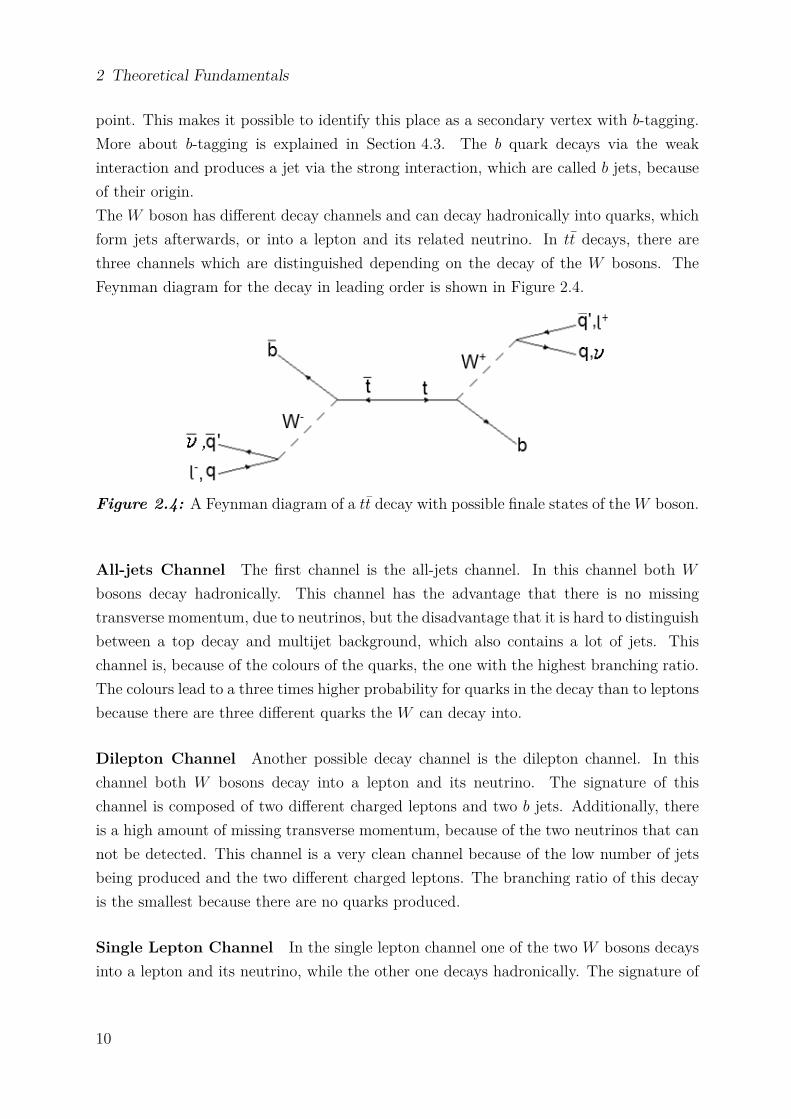
point. This makes it possible to identify this place as a secondary vertex with b-tagging.More about b-tagging is explained in Section 4.3. The b quark decays via the weakinteraction and produces a jet via the strong interaction, which are called b jets, becauseof their origin.The W boson has different decay channels and can decay hadronically into quarks, whichform jets afterwards, or into a lepton and its related neutrino. In tt decays, there arethree channels which are distinguished depending on the decay of the W bosons. TheFeynman diagram for the decay in leading order is shown in Figure 2.4.

Figure 2.4: A Feynman diagram of a tt decay with possible finale states of the W boson.

All-jets Channel The first channel is the all-jets channel. In this channel both W

bosons decay hadronically. This channel has the advantage that there is no missingtransverse momentum, due to neutrinos, but the disadvantage that it is hard to distinguishbetween a top decay and multijet background, which also contains a lot of jets. Thischannel is, because of the colours of the quarks, the one with the highest branching ratio.The colours lead to a three times higher probability for quarks in the decay than to leptonsbecause there are three different quarks the W can decay into.

Dilepton Channel Another possible decay channel is the dilepton channel. In thischannel both W bosons decay into a lepton and its neutrino. The signature of thischannel is composed of two different charged leptons and two b jets. Additionally, thereis a high amount of missing transverse momentum, because of the two neutrinos that cannot be detected. This channel is a very clean channel because of the low number of jetsbeing produced and the two different charged leptons. The branching ratio of this decayis the smallest because there are no quarks produced.

Single Lepton Channel In the single lepton channel one of the two W bosons decaysinto a lepton and its neutrino, while the other one decays hadronically. The signature of

10

2.2 Top Quark

this channel is two b jets and two other jets, and one charged lepton with a high transversemomentum. This decay contains a neutrino, which carries momentum, but which can notbe measured in the detector. But because there is only one neutrino, its momentum canbe reconstructed by the missing transverse momentum.The leptons used in this channel are only electrons and muons and not tau leptons thatis just a convention because it is more difficult to identify tau leptons.In the analysis in the later chapters, single-lepton events are used because of a goodcompromise between a good reconstruction and sufficient statistics.

11

3 Experimental Setup

3.1 Large Hadron Collider

The Large Hadron Collider (Lhc) is a proton-proton collider at CERN in Geneva andnowadays the most powerful collider in the world. Next to proton-proton collisions at Lhcthere is the possibility to collide heavier lead ions. Lhc is a synchrotron with a radiusof about 27 km at approximately 100 m under the ground. It is placed in the tunnelwhere Lep, the Large Electron Positron Collider, was before. Lhc started its operationin March 2010 with a centre-of-mass energy of 7 TeV. In 2012, the centre-of-mass energywas increased to 8 TeV and from spring 2013 until 2015 Lhc has a scheduled downtime.For 2015 and the following years an operation at 13 TeV and 14 TeV is planned. TheLhc was built for the search for the Higgs boson and new physics beyond the StandardModel. In 2012, the Higgs boson could be discovered, as mentioned in Section 2.1.3.The Lhc needs two beam pipes because both beams have the same charge, but need tobe accelerated in different directions, so the particles can not be in the same pipe and thesame magnetic dipole field. To force the particles with 7 TeV on a circular trajectory ina 27 km ring, the magnetic dipole field needs a strength of 8.33 T. Such a high magneticfield can not be reached by normal magnets. That is why superconducting magnets areneeded. In the case of the Lhc, the magnets are built with Nb-Ti, which are cooled withliquid helium to 1.9 K. To accelerate the particles inside the accelerator, superconductingradio frequency cavities are used. In addition, quadrupole magnets are used to focus thebeams [20].At maximum energy one beam contains 2808 bunches of protons, with 1011 protons ineach bunch. The bunches cross all 25 ns.At Lhc, there are four major experiments with their detectors. These detectors are Alice,Atlas, Cms, and Lhcb. Atlas and Cms are multi-purpose detectors, while Alice placesa focus on lead ion collisions and Lhcb focuses on physics with b quarks. The data used inthe analysis is collected with the Atlas detector, which will be explained in more detailin the next section.

13

3 Experimental Setup

3.2 The Atlas Detector

Atlas is an acronym for A Torodial LHC ApparatuS. It is a multi-purpose detectorat the Lhc. Atlas is 44 m long covers 4π in solid angle with a diameter of 25 m anda weight of about 7,000 t. A sketch of the Atlas detector with its components can beseen in Figure 3.1. The detector is composed of different sections, the inner detector, thecalorimeter system, the muon spectrometer and the magnet system.The coordinate system used by the Atlas collaboration is a right-handed Cartesiancoordinate system, with the origin set at the interaction point and the z axis pointingalong the beam direction. The coordinates will be discussed in Chapter 4.5 in more detail.

Figure 3.1: Cut-away view of the Atlas detector [21].

3.2.1 Inner Detector

The inner detector consists of three different sub-detectors, these three are the Pixeldetector, the Semiconductor Tracker (SCT) and the Transition Radiation Tracker (TRT).A solenoid with a length of 5.3 m and a diameter of 2.5 m surrounds the complete innerdetector in a magnetic field of 2 T.The Pixel detector and the SCT are used to distinguish between the interaction point andsecondary vertices, for example for b-tagging purposes. The number of readout channelsin the pixel detector is about 80.4 million and in the SCT about 6.3 million.The TRT is used to determine the momentum of a particle by the curvature of the

14

3.2 The Atlas Detector

particle’s trajectory in the magnetic field, which is mainly used for e − π separation. Forthis sub-detector, there are 315,000 readout channels [21].

3.2.2 Calorimeter System

The calorimeter is used to measure the energy of particles. This is done by depositing allof the particle’s energy in the calorimeter. The particles do not leave the calorimeter after-wards. For the Atlas detector, sampling calorimeters are used. A sampling calorimeterconsists of active and passive material. The energy resolution can be approximated by

σ(E)E

= a√E

⊕ b, (3.1)

where the first term depends on the material used for the calorimeter and the second onehas to be added due to miscalibration, lost energy, etc. The ⊕ means the quadraturesummation of errors [22]. In Atlas, there are two different calorimeters, the electromag-netic calorimeter and the hadronic calorimeter.In the electromagnetic calorimeter, the energies of photons and electrons are measured.The processes of energy deposition are e+e− pair production and Bremsstrahlung. Anelectron, for example, enters the calorimeter and radiates Bremsstrahlung. The photonof the Bremsstrahlung then produces an e+e− pair, which radiates Bremsstrahlung again.By these processes a shower is formed in the calorimeter. The active material is liquidargon and the passive material is lead. The energy resolution of the electromagneticcalorimeter is roughly [23]

σE

E= 10%√

E⊕ 0.7%. (3.2)

The hadronic calorimeter is used to measure the energy of hadronic particles like protons.The passive material in this calorimeter is steel and scintillator the active one [21]. Theenergy resolution in this calorimeter is [23]

σE

E= 50%√

E⊕ 3%. (3.3)

3.2.3 Muon Spectrometer

The energy of muons can not be measured in the electromagnetic calorimeter because theydo not radiate Bremsstrahlung and so they will not be stopped. For those muons, there

15

3 Experimental Setup

is an extra part in the outer layer of the detector. This part is the muon spectrometer.It consists of four different chambers, the Monitored Drift Tube (MDT), Cathode-StripChambers (CSC), Resistive Plate Chambers (RPC) and Thin Gap Chambers (TGC).The first two are used to measure the momenta of muons, while the other two are usedas triggers. The muon spectrometer is immersed in an inhomogeneous toroidal magneticfield of 1 T to bend the trajectory of the muons to measure their momenta [21].

3.2.4 Trigger System

Everytime the beams cross, large amounts of data are provided, but most of the detectedevents are not appreciable. To select between interesting and not so interesting events,a trigger system is used. At the Atlas detector, a three-level trigger system is used toidentify interesting events. If the data would not be selected, it would be impossible tostore all the data.The first trigger is the level-1 trigger L1. It searches for high-pT muons, electrons, photons,jets or hadronically decaying tau leptons and events with large transverse momentum andenergy. The trigger makes fast decisions in about 2.5 µs and defines a region of interest(ROI). The level-2 trigger L2 checks the ROI and reconstructs the event. This triggerhas a processing time of about 40 ms. The last trigger stage is the Event Filter EF thatreconstructs and analyses the event with high precision algorithms, this takes about 4 s.After all three triggers the event is saved permanently.

16

4 Fundamentals of the Analysis

In the detector, just the final state products are observed, but not the initial particles.To figure out what particles were produced in the first place, the final state particles arecompared with the signatures of the decay of interest. However, this signature is notunique due to other processes with the same end products, which are called backgroundprocesses. To get better estimations of those background processes, Monte Carlo simula-tions of the signal and the backgrounds processes, are compared with the measured data.This comparison is often shown in graphical way in the form of control plots.The observed decay channel of tt in this thesis is the single lepton channel, explainedin Section 2.2.3. The signature of this channel consists of at least four jets, with two ofthem being tagged as b jets, a charged lepton, which is not a tau lepton, and a largeamount of missing transverse momentum because of the neutrino in the final state. Sev-eral background processes have the same signature, they will be discussed in the followingsection.

4.1 Background Processes

The background processes for the single lepton tt decay are W+ jets and Z+ jets, aswell as diboson processes with two weak bosons, so WW , ZZ and ZW events. Otherbackground processes are single top decays and multijet events. Some of these processescontain a W boson which decays leptonically. These processes are the WW and ZW

diboson background processes, the single top and the W+ jets background. The missingtransverse momentum in these processes is caused by the neutrino from the leptonic W

decay. In the multijet background, also called QCD background or misidentified leptonbackground, the lepton is faked by a jet and the missing transverse momentum comesfrom incomplete reconstruction of the jets or leptons. In the Z+ jets process, the Z

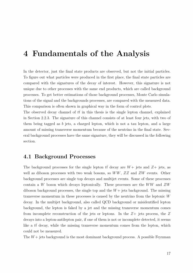
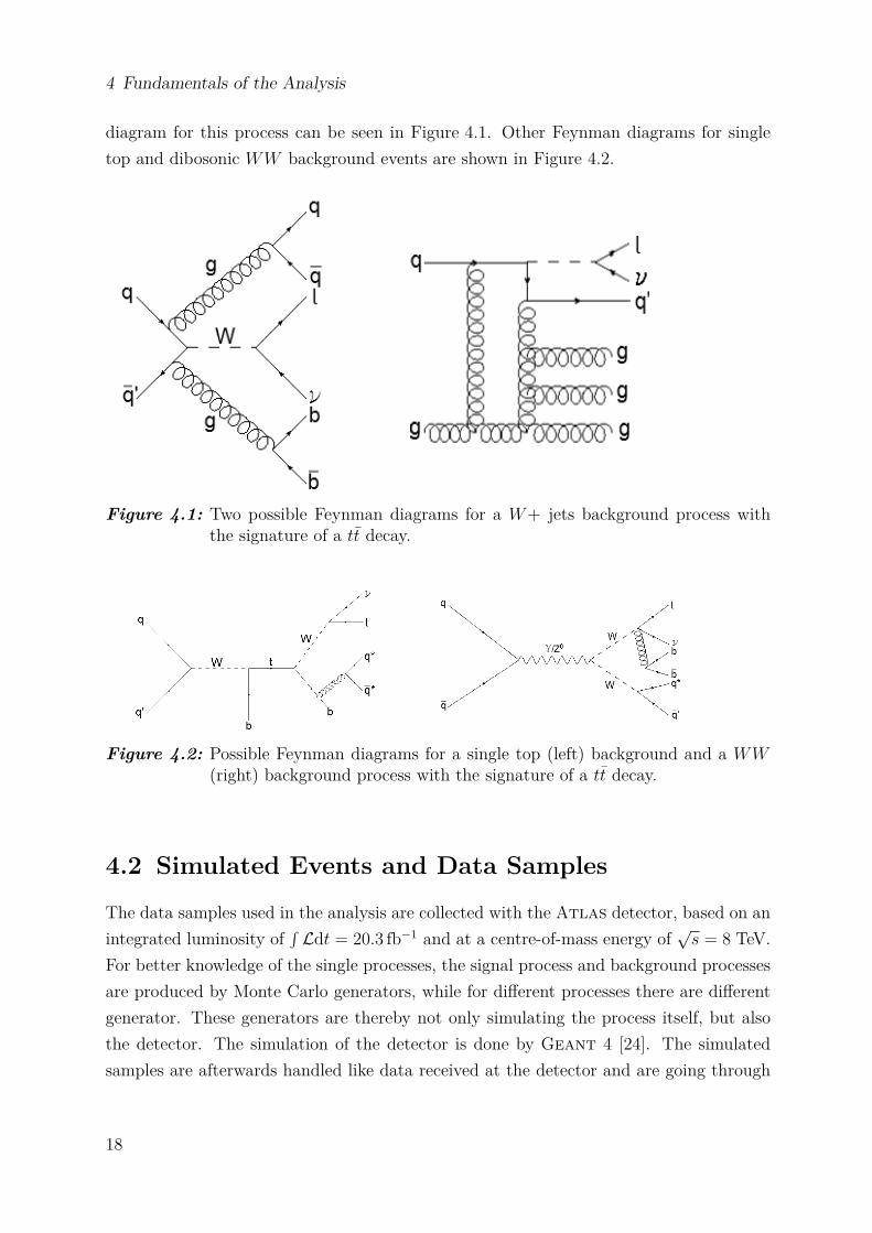
decays into a lepton-antilepton pair, if one of them is not or incomplete detected, it seemslike a tt decay, while the missing transverse momentum comes from the lepton, whichcould not be measured.The W+ jets background is the most dominant background process. A possible Feynman

17

4 Fundamentals of the Analysis

diagram for this process can be seen in Figure 4.1. Other Feynman diagrams for singletop and dibosonic WW background events are shown in Figure 4.2.

Figure 4.1: Two possible Feynman diagrams for a W+ jets background process withthe signature of a tt decay.

Figure 4.2: Possible Feynman diagrams for a single top (left) background and a WW(right) background process with the signature of a tt decay.

4.2 Simulated Events and Data Samples

The data samples used in the analysis are collected with the Atlas detector, based on anintegrated luminosity of

∫Ldt = 20.3 fb−1 and at a centre-of-mass energy of

√s = 8 TeV.

For better knowledge of the single processes, the signal process and background processesare produced by Monte Carlo generators, while for different processes there are differentgenerator. These generators are thereby not only simulating the process itself, but alsothe detector. The simulation of the detector is done by Geant 4 [24]. The simulatedsamples are afterwards handled like data received at the detector and are going through

18

4.3 b-Tagging

the same analysis chain [25].The simulated signal is produced with the Monte Carlo event generators Powheg [26, 27]and Pythia [28]. The events for the W+ jets, Z+ jets and the diboson background aresimulated by the generator Alpgen [29] and Pythia. Some missing contributions inthe dibosonic background are simulated with Sherpa [30]. The single top backgroundis simulated, like the signal, with Powheg and Pythia and events in the t-channel aregenerated by AcerMC [31] and Pythia.The multijet background is not simulated by a Monte Carlo generator but estimated usingthe data. This estimation is done using a matrix method [32, 33].

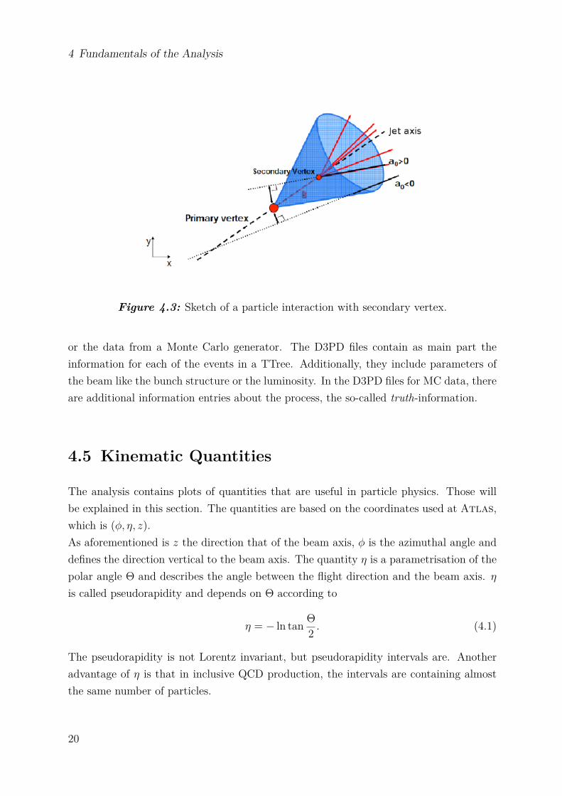
4.3 b-Tagging

In the tt decay the two b jets are a very necessary part of the signature, because theyare not that likely in background processes. Therefore it is very useful to have a goodidentification of these jets. As mentioned before, the b jets are identified by b-tagging. Ajet out of other jets that is identified as a b jet is called tagged. The b quarks are formingmesons with other quarks, these mesons are B mesons. All these mesons containing a b

quark have a comparatively long lifetime of a few ps [1]. The long lifetime is leading toa measureable flight length of a few millimetre and so to an observable secondary vertex[34]. A sketch of the idea of b-tagging can be found in Figure 4.3.The easiest method of b-tagging is to call a jet a b jet if the impact parameter, defined asthe distance between the interaction point and the point of closest approach, of a certainnumber of tracks is above a certain value.In this analysis, the b-tagger is the MV1-tagger used at Atlas. This tagger combines theinformation of three different high-performance taggers that use likelihood ratios. Thesethree taggers are IP3D, JetFitter and SV1. The IP3D is an impact parameter based taggerusing the significances of the impact parameter in longitudinal and transverse direction.The JetFitter finds a line which includes the interaction point and the secondary vertex.Finally, the SV1 is based on the secondary vertices formed by B meson decays [34]. TheMV1 is used with a weight of 0.7892, which corresponds to an efficiency working point of70%.

4.4 D3PD

The Derived Physics Data (D3PD) are the data files used for analysis in Atlas. Thesefiles are produced from the RAW data, which are the files received from the detector

19

4 Fundamentals of the Analysis

Figure 4.3: Sketch of a particle interaction with secondary vertex.

or the data from a Monte Carlo generator. The D3PD files contain as main part theinformation for each of the events in a TTree. Additionally, they include parameters ofthe beam like the bunch structure or the luminosity. In the D3PD files for MC data, thereare additional information entries about the process, the so-called truth-information.

4.5 Kinematic Quantities

The analysis contains plots of quantities that are useful in particle physics. Those willbe explained in this section. The quantities are based on the coordinates used at Atlas,which is (ϕ, η, z).As aforementioned is z the direction that of the beam axis, ϕ is the azimuthal angle anddefines the direction vertical to the beam axis. The quantity η is a parametrisation of thepolar angle Θ and describes the angle between the flight direction and the beam axis. η

is called pseudorapidity and depends on Θ according to

η = − ln tan Θ2

. (4.1)

The pseudorapidity is not Lorentz invariant, but pseudorapidity intervals are. Anotheradvantage of η is that in inclusive QCD production, the intervals are containing almostthe same number of particles.

20

4.5 Kinematic Quantities

Distances in the η − ϕ plane are called ∆R and are given by

∆R =√

∆η2 + ∆ϕ2. (4.2)

As mentioned in Section 2.2.2, the longitudinal momentum of a particle is unknown, butthe transverse momentum pT of the partons inside the hadron has to be 0, otherwise theparticle would split apart. Due to momentum conservation, the transverse momentumafter the interaction has to be 0 again. Therefore the transverse momentum is used todescribed the motion of particles. A quantity linked to the transverse momentum is themissing transverse momentum ET . This is the momentum that is missing to have a totalmomentum of 0. This momentum is carried by neutrinos and is used to describe theirmomentum.In combination with the energy E or the mass M of a particle, pT , η and ϕ are buildingan alternative four-vector that describes a particle.

21

5 TopRootCore

5.1 The Software Package TopRootCore

TopRootCore is a software package based on RootCore, which depends on Root. Root isan object-oriented programme, which was designed for data analysis in particle physics.It is written in C++ and was designed for the needs to analyse the data of the LHC [35].RootCore is a software package used by the different groups at Atlas to make the resultseasier to compare because not every group uses its own package. TopRootCore therebyis specified for the analysis needed for the top group. In TopRootCore, it is possible toimplement additional packages depending on the analysis.TopRootCore uses D3PD datasets, which are available for all Atlas groups. There areD3PD datasets for Monte Carlo generated events and collision data. The data used forthe analysis in Chapter 6 are the NTUP_TOP files. TopRootCore uses the D3PD filesas input files and applies different event selections. Also estimations of the backgroundsand systematic uncertainties are performed. The output file is a Root file, which can beopened with Root.In this analysis, the TopRootCore version 14-00-23 was used, which has several recom-mended cuts. Not included in this version are cuts on the missing transverse momentumand on the transverse mass of the W boson.

5.2 PlotFactory

The PlotFactory is a package implemented in TopRootCore. It was developed by the topgroup of the university in Göttingen. It uses the output files of TopRootCore and producescontrol plots. The PlotFactory package can be separated in two parts, the HistoCreatorand the PlotFactory part itself. The HistoCreator takes the Root files, which are theoutput files of TopRootCore, and produces new Root files for different jet and b-tagoptions. The options are initialised in the Python script, which runs the HistoCreator.The chosen option for jets is the “4incl.”, what means that there are at least four jets. Forthe b-tags there are more possibilities, these are “0excl., 1excl., 2excl., 0incl., 1incl.” and

23

5 TopRootCore

“2incl.”, while exclusive means that there are exactly 0, 1 or 2 jets with a MV1 weightlarger than 0.7892 and which means they are tagged as b jets. For the inclusive option,there are more than 0, 1 or 2 jets tagged as b jets.The analysis of the data is also done in the HistoCreator, while these analyses are donein external files to give a better overview of the single analysis steps. The different filesmake it easier to modify or add single analysis steps.The quantities for the analysis are saved in TH1D histograms and depending on theirorigin, saved in different Root files and different folders, which contain information ofthe number of jets and the number of b-tags. Additionally, the Python script has theoption of activating or deactivating single background processes, for example, to give thepossibility to run the programme faster to see changes in the output files.The PlotFactory takes the output files of the HistoCreator and fills their informationinto control plots. There are control plots for different b-tag options and also for thetwo lepton possibilities, so electrons or muons. In addition to the control plots, thePlotFactory produces an HTML file, where all plots are presented. Again, there are twodifferent HTML files for the same b-tag options, one for the electron channel and onefor the muon channel. Next to the plots, the HTML files contain the event yield tables,were the numbers of events for the data, simulated signal and the different backgroundprocesses are shown. These numbers are calculated by summing the bin contents of thesingle bins for a process in the Root files produced by the HistoCreator.The control plots show the different simulated processes as coloured boxes and producesa Root object, called stack, of these boxes by batching them on each other. The detectordata is included as points. Additionally to the information of the processes, parametersof the detector like the integrated luminosity

∫Ldt are included, as well as a legend

containing the colour code, explaining which colour belongs to which process.

24

6 Results

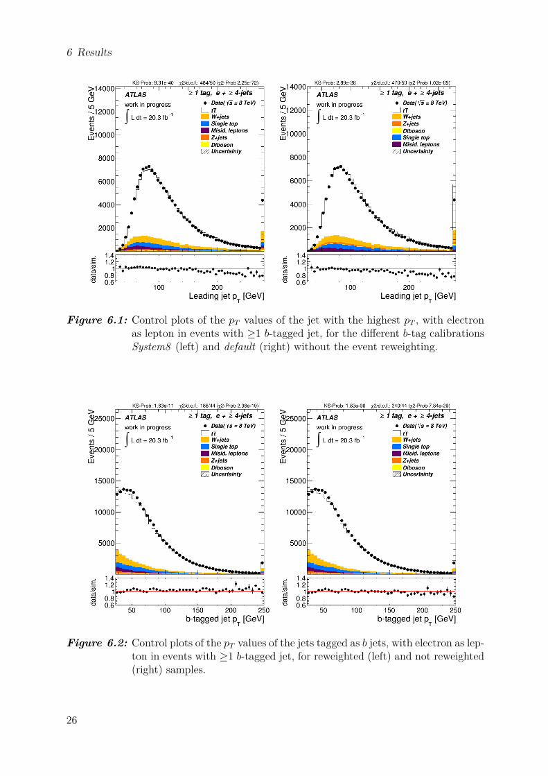
This bachelor project was to modify the PlotFactory package implemented in TopRoot-Core as introduced in Section 5.2. There were four major modifications added to thePlotFactory package. These changes were to renew the HTML page produced by thePlotFactory to present the plots in a clearer way. The implementation of plots for PseudoTop related distributions. Another project was to add goodness-of-fit tests, the χ2 andKolmogorow-Smirnow tests to the analysis and displayed them in the plots. Anothermodification was to produce a plot with logarithmic y axis for all quantities. The changesare applied for the group project of measureing the decay width of the top quark. Also,the progress of the group project will be displayed.During the project, a discrepancy in the selected events could be observed. The progressof improving this discrepancy will be shown, however, investigating the reasons for thediscrepancy is not part of this analysis. The displayed plots in the analysis are for the elec-tron channel, for reasons of completeness some muon plots are included in Appendix A.To compare the results with results of other groups, additional cuts were applied to theanalysis. These cuts were applied on the missing transverse momentum and the trans-verse mass of the W boson. The missing transverse momentum cut is ET > 30 GeV andthe transverse mass cut MT > 30 GeV. For the same reason another b-tag calibration wasused. In addition to the b-tag calibration recommended in TopRootCore, System8 [36],the calibration method default was tested. Exemplary control plots for the different b-tagcalibration options can be seen in Figure 6.1. The System8 method uses three selectioncriteria, which are uncorrelated to a data sample with a muon associated with a jet tobuild a system of eight equations to serve as calibration for the b-tagger. The defaultmethod uses tt events to calibrate the b-tagger. The plots show the pT values of the jetwith the highest pT in each event. If not mentioned otherwise, for all plots the System8calibration was used.

25

6 Results

Figure 6.1: Control plots of the pT values of the jet with the highest pT , with electronas lepton in events with ≥1 b-tagged jet, for the different b-tag calibrationsSystem8 (left) and default (right) without the event reweighting.

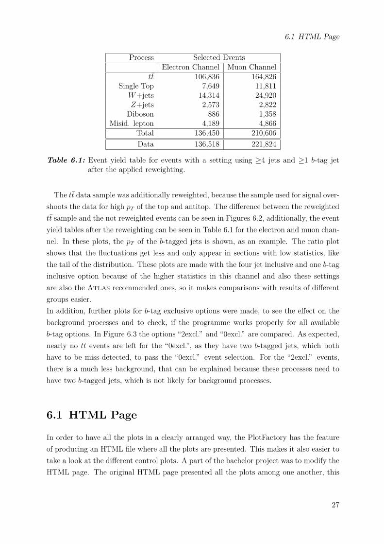
Figure 6.2: Control plots of the pT values of the jets tagged as b jets, with electron as lep-ton in events with ≥1 b-tagged jet, for reweighted (left) and not reweighted(right) samples.

26

6.1 HTML Page

Process Selected EventsElectron Channel Muon Channel

tt 106,836 164,826Single Top 7,649 11,811

W+jets 14,314 24,920Z+jets 2,573 2,822

Diboson 886 1,358Misid. lepton 4,189 4,866

Total 136,450 210,606Data 136,518 221,824

Table 6.1: Event yield table for events with a setting using ≥4 jets and ≥1 b-tag jetafter the applied reweighting.

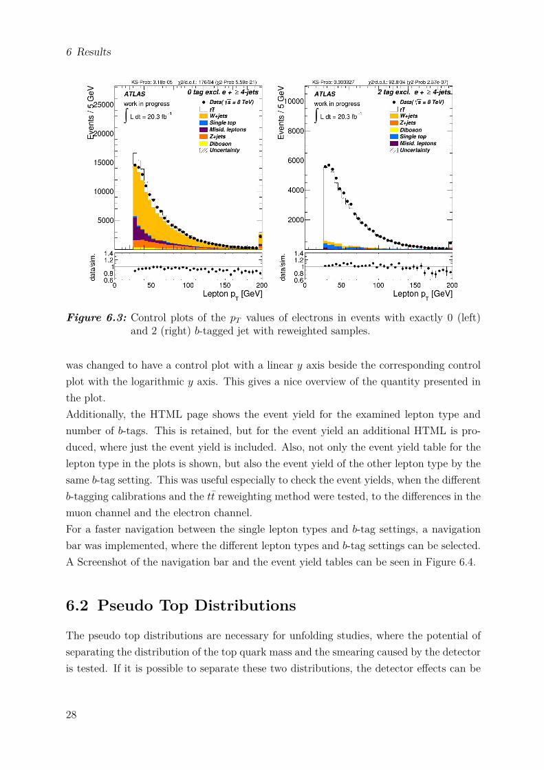
The tt data sample was additionally reweighted, because the sample used for signal over-shoots the data for high pT of the top and antitop. The difference between the reweightedtt sample and the not reweighted events can be seen in Figures 6.2, additionally, the eventyield tables after the reweighting can be seen in Table 6.1 for the electron and muon chan-nel. In these plots, the pT of the b-tagged jets is shown, as an example. The ratio plotshows that the fluctuations get less and only appear in sections with low statistics, likethe tail of the distribution. These plots are made with the four jet inclusive and one b-taginclusive option because of the higher statistics in this channel and also these settingsare also the Atlas recommended ones, so it makes comparisons with results of differentgroups easier.In addition, further plots for b-tag exclusive options were made, to see the effect on thebackground processes and to check, if the programme works properly for all availableb-tag options. In Figure 6.3 the options “2excl.” and “0excl.” are compared. As expected,nearly no tt events are left for the “0excl.”, as they have two b-tagged jets, which bothhave to be miss-detected, to pass the “0excl.” event selection. For the “2excl.” events,there is a much less background, that can be explained because these processes need tohave two b-tagged jets, which is not likely for background processes.

6.1 HTML Page

In order to have all the plots in a clearly arranged way, the PlotFactory has the featureof producing an HTML file where all the plots are presented. This makes it also easier totake a look at the different control plots. A part of the bachelor project was to modify theHTML page. The original HTML page presented all the plots among one another, this

27

6 Results

Figure 6.3: Control plots of the pT values of electrons in events with exactly 0 (left)and 2 (right) b-tagged jet with reweighted samples.

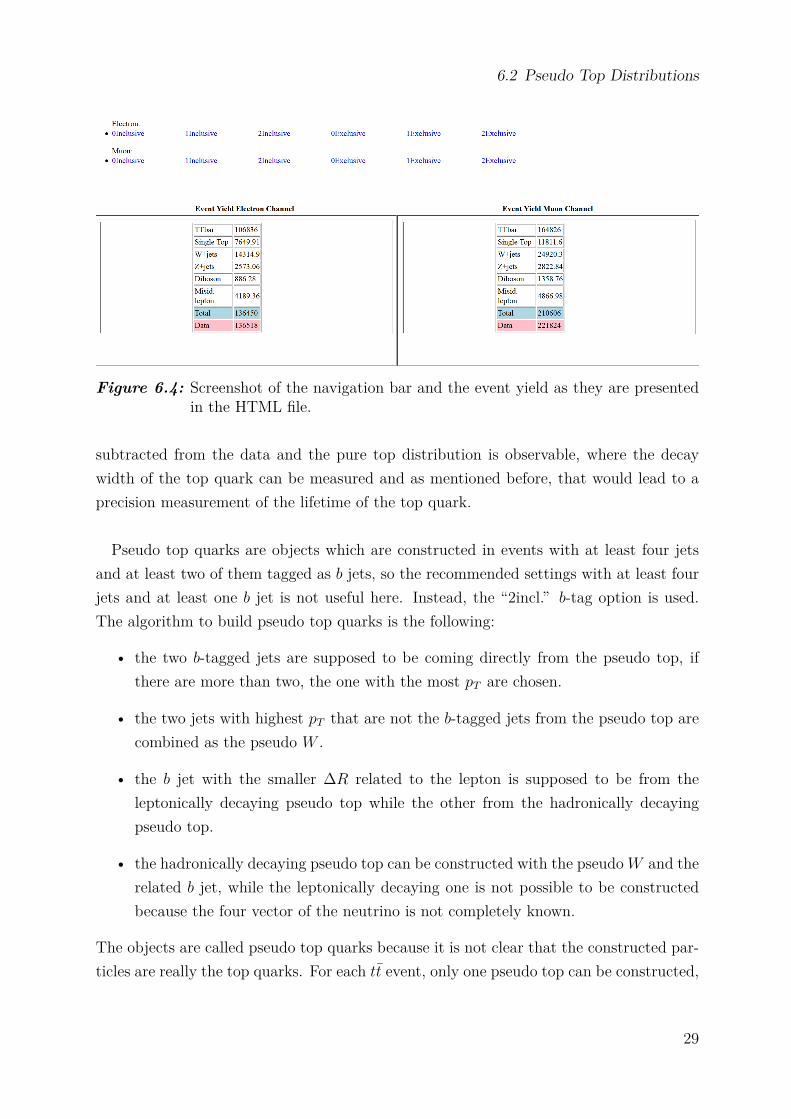
was changed to have a control plot with a linear y axis beside the corresponding controlplot with the logarithmic y axis. This gives a nice overview of the quantity presented inthe plot.Additionally, the HTML page shows the event yield for the examined lepton type andnumber of b-tags. This is retained, but for the event yield an additional HTML is pro-duced, where just the event yield is included. Also, not only the event yield table for thelepton type in the plots is shown, but also the event yield of the other lepton type by thesame b-tag setting. This was useful especially to check the event yields, when the differentb-tagging calibrations and the tt reweighting method were tested, to the differences in themuon channel and the electron channel.For a faster navigation between the single lepton types and b-tag settings, a navigationbar was implemented, where the different lepton types and b-tag settings can be selected.A Screenshot of the navigation bar and the event yield tables can be seen in Figure 6.4.

6.2 Pseudo Top Distributions

The pseudo top distributions are necessary for unfolding studies, where the potential ofseparating the distribution of the top quark mass and the smearing caused by the detectoris tested. If it is possible to separate these two distributions, the detector effects can be

28

6.2 Pseudo Top Distributions

Figure 6.4: Screenshot of the navigation bar and the event yield as they are presentedin the HTML file.

subtracted from the data and the pure top distribution is observable, where the decaywidth of the top quark can be measured and as mentioned before, that would lead to aprecision measurement of the lifetime of the top quark.

Pseudo top quarks are objects which are constructed in events with at least four jetsand at least two of them tagged as b jets, so the recommended settings with at least fourjets and at least one b jet is not useful here. Instead, the “2incl.” b-tag option is used.The algorithm to build pseudo top quarks is the following:

• the two b-tagged jets are supposed to be coming directly from the pseudo top, ifthere are more than two, the one with the most pT are chosen.

• the two jets with highest pT that are not the b-tagged jets from the pseudo top arecombined as the pseudo W .

• the b jet with the smaller ∆R related to the lepton is supposed to be from theleptonically decaying pseudo top while the other from the hadronically decayingpseudo top.

• the hadronically decaying pseudo top can be constructed with the pseudo W and therelated b jet, while the leptonically decaying one is not possible to be constructedbecause the four vector of the neutrino is not completely known.

The objects are called pseudo top quarks because it is not clear that the constructed par-ticles are really the top quarks. For each tt event, only one pseudo top can be constructed,

29

6 Results

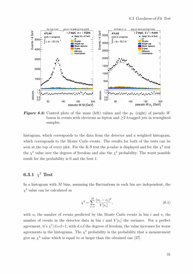
because the neutrino can not be fully reconstructed without making conclusions on theresult. A possible way to reconstruct the neutrino would be to force the sum of the leptonand the neutrino to build an object with the mass of the W boson.The results of these analyses are shown in Figure 6.5, where it can be seen that the peakof the mass is near the value of the mass of the top quark. In addition, the control plotsof the pT and mass of the hadronically decaying pseudo W boson, which can also beconstructed, are shown in Figure 6.6. Also in this plots, it can be seen that the mass peakis at the expected place, so close to the mass of the W boson.

Figure 6.5: Control plots of the mass (left) values and the pT (right) of pseudo topquarks in events with electrons as lepton and ≥2 b-tagged jets in reweightedsamples.

6.3 Goodness-of-Fit Test

For a comparison of data taken by a detector quantify data produced by a Monte Carlogenerator, it is necessary to have methods to proof their agreement. This is accomplishedby goodness-of-fit tests which compare for example data points with a regression functionor in this case simulated data. There are a lot of different goodness-of-fit tests and twoof them were implemented in the PlotFactory, in this bachelor project. These two are theKolmogorow-Smirnow (K-S) test and the χ2 test. For both, a short explanation will begiven later in this section. The χ2 test is implemented as a comparison of an unweighted

30

6.3 Goodness-of-Fit Test

Figure 6.6: Control plots of the mass (left) values and the pT (right) of pseudo Wboson in events with electrons as lepton and ≥2 b-tagged jets in reweightedsamples.

histogram, which corresponds to the data from the detector and a weighted histogram,which corresponds to the Monte Carlo events. The results for both of the tests can beseen at the top of every plot. For the K-S test the p-value is displayed and for the χ2 testthe χ2 value over the degrees of freedom and also the χ2 probability. The worst possibleresult for the probability is 0 and the best 1.

6.3.1 χ2 Test

In a histogram with M bins, assuming the fluctuations in each bin are independent, theχ2 value can be calculated as

χ2 =M∑

i=1

(ni − vi)2

V [vi], (6.1)

with ni the number of events predicted by the Monte Carlo events in bin i and vi thenumber of events in the detector data in bin i and V [vi] the variance. For a perfectagreement, it’s χ2/d.o.f=1, with d.o.f the degrees of freedom, the value increases for worseagreements in the histograms. The χ2 probability is the probability that a measurementgive an χ2 value which is equal to or larger than the obtained one [37].

31

6 Results

6.3.2 Kolmogorow-Smirnow Test

The K-S test is based on an empirical cumulative distribution function FN(x), with N thenumber of measurements of an observable. This can be compared with another cumulativedistribution function F (x). The largest distance between these two function DN is givenby

DN = max|FN(x) − F (x)|. (6.2)

The value√

NDN defines the critical region for the K-S test, for a perfect agreementapplies DN = 0 and increases for less agreement. The K-S test can also be used for datawith low statistics [37].

6.4 Logarithmic Scale Plots

In regions with low statistics and backgrounds, which are not as likely, the visibility isvery low. To amplify the visibility, it is necessary to add plots with a logarithmic y axis,so that no details are overlooked. The used logarithm is the one to the base 10. Forthe maximal value on the y axis a high value was chosen to avoid the histograms overlapwith the legend, so the histograms and the legend are still readable without problems.The minimal value was chosen by taking the smallest background and for this smallestbackground the smallest entry while still being larger than 0. Because of the weighting ofthe generated processes, this value can be smaller than 1. If the smallest entry is found,the minimum for the y axis is the order of this value minus one. This way, the minimumis not chosen arbitrarily. An example for a plot with logarithmic scale and the advantagefor regions with low statistics can be seen in Figure 6.7 in plots with the pT values for alljets, because this quantity has a long tail.In the plots themselves, the backgrounds are sorted by the number of events they have inthe 4 jets inclusive and 1 b jet inclusive setting. So the dibosonic background, which hasthe least number of events, is at the bottom of the plot, above is the Z+ jets background.On top of them is the multijet background, followed by the single top background andthe background with the most events is W+ jets background, which is at the top of thecoloured histograms.

32

6.5 Modifications of the Layout

Figure 6.7: Control plots for the pT values of all jets with normal linear y axis (left)and logarithmic y axis (right) in events with electrons as lepton and ≥1b-tagged jet in reweighted samples.

6.5 Modifications of the Layout

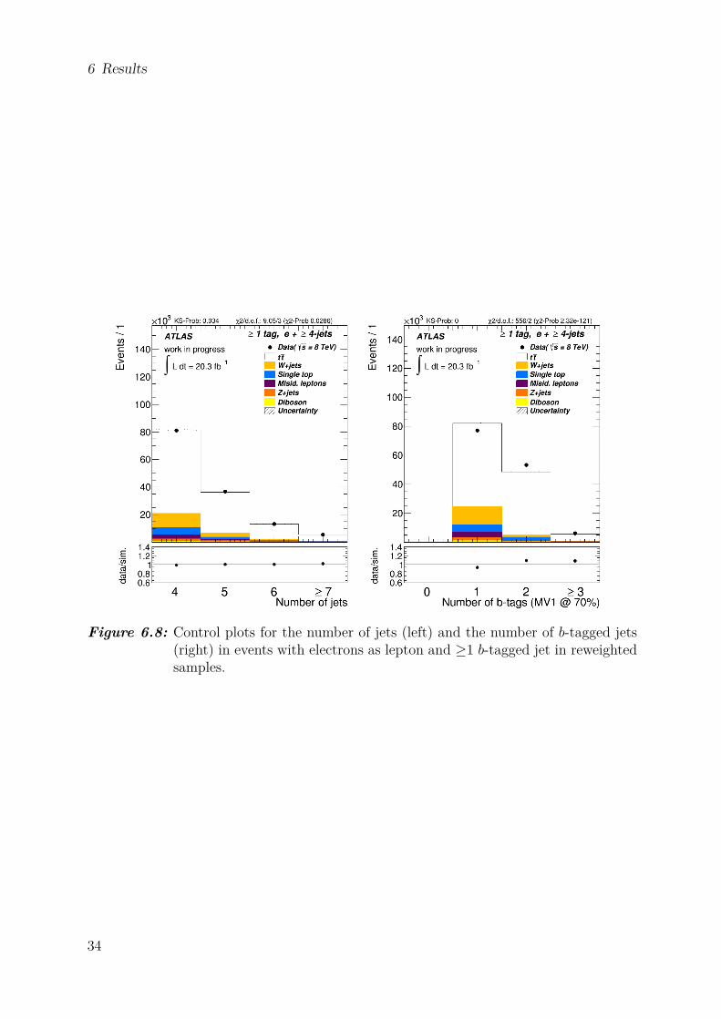
During the project, different modifications on the layout of the control plots have beenmade. These were, for example, to change the legend that way that the events aredisplayed in the order they have in the plots. Also, the value of the integrated luminositywas set to the current value and the x axis label of the plots showing the number of jetsand the number of b-tagged jets. The changes in the axis labels were to illustrate thatthe last bin contains additionally the overflow bin and so, not just the events with 7 jetor 3 b-tagged jets. The plots for the number of jets and the number of b-tagged jets canbe seen in Figure 6.8.

33

6 Results

Figure 6.8: Control plots for the number of jets (left) and the number of b-tagged jets(right) in events with electrons as lepton and ≥1 b-tagged jet in reweightedsamples.

34

7 Conclusion

The main part of the bachelor project was to modify the PlotFactory package, which isimplemented in TopRootCore and is used to produce control plots. The modificationsdone included a renewed HTML page that now contains additional information and plotsthat are arranged in a clearer way. Also, the navigation between the different lepton typesand b-tag settings has been improved.The pseudo top construction included in the analysis, shows a peak near the mass of thetop quark and also the pseudo W mass peak is in the expected region. So these resultscan be used for additional studies to measure the decay width of the top quark.The logarithmic scales simplify observations of smaller backgrounds and in regions withlow statistics so that nothing is overlooked.The goodness-of-fit tests make it possible to see if there is a good comparison betweenthe data recorded at the detector and the events produced with Monte Carlo generators,without the subjective component of judging the agreement by eye.During the studies, several smaller bugs inside the PlotFactory package were found andfixed, even apart from the modified parts of the programme.The PlotFactory produces and presents the control plots now in a clearer way.

35

A Additional Plots

37

A Additional Plots

Figure A.1: Control plots of the pT values of the jet with thge highest pT , for muonin events with ≥1 b-tagged jet, for the different b-tag calibrations System8(left) and default (right) without the event reweight.

Figure A.2: Control plots of the pT values of the jets tagged as b jets, with muonsas lepton in events with ≥1 b-tagged jet, for reweighted (left) and notreweighted (right) samples.

38

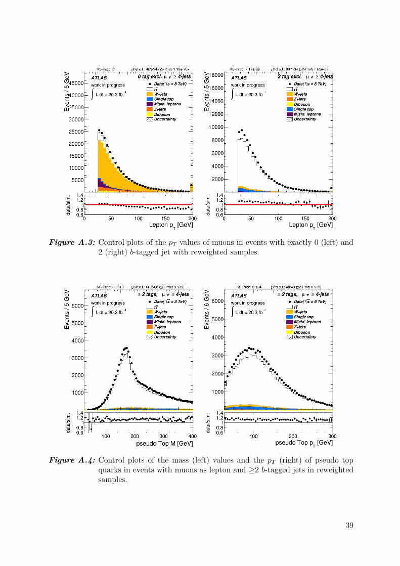
Figure A.3: Control plots of the pT values of muons in events with exactly 0 (left) and2 (right) b-tagged jet with reweighted samples.

Figure A.4: Control plots of the mass (left) values and the pT (right) of pseudo topquarks in events with muons as lepton and ≥2 b-tagged jets in reweightedsamples.

39

A Additional Plots

Figure A.5: Control plots of the mass (left) values and the pT (right) of pseudo Wboson in events with muons as lepton and ≥2 b-tagged jets in reweightedsamples.

Figure A.6: Control plots for the pT values of all jets with normal linear y axis (left) andlogarithmic y axis (right) in events with muons as lepton and ≥1 b-taggedjet in reweighted samples.

40

Figure A.7: Control plots for the number of jets (left) and the number of b-tagged jets(right) in events with muons as lepton and ≥1 b-tagged jet in reweightedsamples.

41

Bibliography

[1] J. Beringer, et al. (Particle Data Group), Review of Particle Physics, Phys. Rev. D86, 010001 (2012)

[2] M. Kobayashi, T. Maskawa, CP Violation in the Renormalizable Theory of WeakInteraction, Prog. Theor. Phys. 49, 652 (1973)

[3] N. Cabibbo, Unitary Symmetry and Leptonic Decays, Phys. Rev. Lett. 10, 531 (1963)

[4] S. Glashow, Partial Symmetries of Weak Interactions, Nucl. Phys. 22, 579 (1961)

[5] A. Salam, J. C. Ward, Weak and electromagnetic interactions, Nuovo Cim. 11, 568(1959)

[6] S. Weinberg, A Model of Leptons, Phys. Rev. Lett. 19, 1264 (1967)

[7] P. W. Higgs, Broken Symmetries and the Masses of Gauge Bosons, Phys. Rev. Lett.13, 508 (1964)

[8] F. Englert, R. Brout, Broken Symmetry and the Mass of Gauge Vector Mesons, Phys.Rev. Lett. 13, 321 (1964)

[9] G. Guralnik, C. Hagen, T. Kibble, Global Conservation Laws and Massless Particles,Phys. Rev. Lett. 13, 585 (1964)

[10] ATLAS Collaboration (G. Aad, et al.), Observation of a new particle in the searchfor the Standard Model Higgs boson with the ATLAS detector at the LHC, Phys. Lett.B716, 1 (2012)

[11] CMS Collaboration, Observation of a new boson at a mass of 125 GeV with the CMSexperiment at the LHC, Phys. Lett. B716, 30 (2012)

[12] CDF Collaboration (T. Aaltonen, et al.), Observation of top quark production in pp

collisions, Phys. Rev. Lett. 74, 2626 (1995)

43

Bibliography

[13] DØ Collaboration (V.M. Abazov, et al.), Observation of the top quark, Phys. Rev.Lett. 74, 2632 (1995)

[14] CDF Collaboration (T. Aaltonen, et al.), First Observation of Electroweak SingleTop Quark Production, Phys. Rev. Lett. 103, 092002 (2009)

[15] DØ Collaboration (V.M. Abazov, et al.), Observation of Single Top Quark Produc-tion, Phys. Rev. Lett. 103, 092001 (2009)

[16] ATLAS Collaboration (G. Aad, et al.), Measurement of the top quark charge in pp

collisions at√

s = 7 TeV with the ATLAS detector, JHEP 1311, 031 (2013)

[17] ATLAS Collaboration, CDF Collaboration, CMS Collaboration, DØ Collabora-tion, First combination of Tevatron and LHC measurements of the top-quark mass,ATLAS-CONF-2014-008, CDF-NOTE-11071, CMS-PAS-TOP-13-014, D0-NOTE-6416 (2014)

[18] T. Liss, A. Quadt (Particle Data Group), Review of Particle Physics: The Top Quark,Phys. Rev. D 86, 010001 (2012)

[19] J. Pumplin, et al., New generation of parton distributions with uncertainties fromglobal QCD analysis, JHEP 0207, 012 (2002)

[20] O. S. Bruning, et al., LHC Design Report. 1. The LHC Main Ring, CERN-2004-003-V-1, CERN-2004-003 (2004)

[21] ATLAS Collaboration (G. Aad, et al.), The ATLAS Experiment at the CERN LargeHadron Collider, JINST 3, S08003 (2008)

[22] C. Berger, Elementarteilchenphysik: Von den Grundlagen zu den modernen Experi-menten, Springer-Lehrbuch, Springer (2006)

[23] ATLAS Collaboration (G. Aad, et al.), ATLAS: Detector and physics performancetechnical design report. Volume 1, CERN (1999)

[24] S. Agostinelli, et al. (GEANT4), GEANT4: A Simulation toolkit, Nucl. Instrum.Meth. A506, 250 (2003)

[25] ATLAS Collaboration (G. Aad, et al.), The ATLAS Simulation Infrastructure, Eur.Phys. J. C70, 823 (2010)

44

Bibliography

[26] G. Corcella, et al., HERWIG 6.5 release note, CAVENDISH-HEP-02-17, DAMTP-2002-124, KEK-TH-850, MPI-PHT-2002-55, CERN-TH-2002-270, IPPP-02-58, MC-TH-2002-7 (2002)

[27] G. Corcella, et al., HERWIG 6: An Event generator for hadron emission reactionswith interfering gluons (including supersymmetric processes), JHEP 0101, 010 (2001)

[28] T. Sjostrand, et al., PYTHIA 6.4 Physics and Manual, JHEP 0605, 026 (2006)

[29] M. L. Mangano, et al., ALPGEN, a generator for hard multiparton processes inhadronic collisions, JHEP 0307, 001 (2003)

[30] T. Gleisberg, et al., Event generation with SHERPA 1.1, JHEP 0902, 007 (2009)

[31] B. P. Kersevan, E. Richter-Was, The Monte Carlo event generator AcerMC versions2.0 to 3.8 with interfaces to PYTHIA 6.4, HERWIG 6.5 and ARIADNE 4.1, Comput.Phys. Commun. 184, 919 (2013)

[32] B. Abi, et al., Mis-identified lepton backgrounds to top quark pair production, ATL-COM-PHYS-2010-849 (2010)

[33] K. Becker, et al., Mis-identified lepton backgrounds in top quark pair production stud-ies for EPS 2011 analyses, ATL-COM-PHYS-2011-768, (2011)

[34] M. Lehmacher, b-Tagging Algorithms and their Performance at ATLAS,arXiv:0809.4896v3 [hep-ex] (2008)

[35] R. Brun, F. Rademakers, ROOT: An object oriented data analysis framework, Nucl.Instrum. Meth. A389, 81 (1997)

[36] ATLAS Collaboration (G. Aad, et al.), b-Jet Tagging Efficiency Calibration usingthe System8 Method, ATLAS-CONF-2011-143 (2011)

[37] O. Behnke, K. Kröninger, G. Schott, T. Schörner-Sadenius, Data Analysis in HighEnergy Physics: A Practical Guide to Statistical Methods, Wiley (2013)

45

Acknowledgements

First, I would like to thank Prof. Dr. Arnulf Quadt for giving me the opportunity towrite my bachelor’s thesis in particle physics and also for being the first referee. I am alsovery thankful to Prof. Dr. Ariane Frey for being the second referee and for awakeningmy interest in particle physics by giving very inspiring lectures.

I also would like to thank Priv.-Doz. Kevin Kröninger for supervising me and discussingthe achieved results and proof-reading my thesis. His ability to make physics understand-able is incomparable.A thousand thanks to Philipp Stolte for being my supervisor and always being availablewhen I needed help. Also for his patience when solving problems or proof-reading thisthesis. Thank you so much!Additional thanks go to Dominik Müller for helping to start into the project and alwaysknowing the answer to the problems appearing while programming.

47

Erklärung nach §13(8) der Prüfungsordnung für den Bachelor-StudiengangPhysik und den Master-Studiengang Physik an der UniversitätGöttingen:

Hiermit erkläre ich, dass ich diese Abschlussarbeit selbständig ver-fasst habe, keine anderen als die angegebenen Quellen und Hilfsmit-tel benutzt habe und alle Stellen, die wörtlich oder sinngemäß ausveröffentlichten Schriften entnommen wurden, als solche kenntlichgemacht habe.Darüberhinaus erkläre ich, dass diese Abschlussarbeit nicht, auchnicht auszugsweise, im Rahmen einer nichtbestandenen Prüfung andieser oder einer anderen Hochschule eingereicht wurde.

Göttingen, den 18. Juli 2014

(Jens Oltmanns)