STUDIES ON PERFORMANCE OF AN AIRFOIL AND ITS SIMULATION

Dissertation Submitted In Partial Fulfilment of the

Prerequisites for the Degree Of

Masters of Technology

In

Civil Engineering

(Water Resources Engineering)

BY

Rajendra Roul

Roll. No- 213CE4108

Under the supervision of

Prof. Awadhesh Kumar

DEPARTMENT OF CIVIL ENGINEERING

NATIONAL INSTITUTE OF TECHNOLOGY

ROURKELA-769008

MAY, 2015

STUDIES ON PERFORMANCE OF AN AIRFOIL AND ITS SIMULATION

Dissertation Submitted In Partial Fulfilment of the

Prerequisites for the Degree Of

Masters of Technology

In

Civil Engineering

(Water Resources Engineering)

BY

Rajendra Roul

Roll. No- 213CE4108

Under the supervision of

Prof. Awadhesh Kumar

DEPARTMENT OF CIVIL ENGINEERING

NATIONAL INSTITUTE OF TECHNOLOGY

ROURKELA-769008

MAY, 2015

DEPARTMENT OF CIVIL ENGINEERING

NATIONAL INSTITUTE OF TECHNOLOGY,

ROURKELA

DECLARATION I hereby declare that dissertation report entitled “studies on the performance of an airfoil and its simulation” submitted by me to NATIONAL INSTITUTE OF TECHNOLOGY,ROURKELA is a record of original work done by me under the guidance of prof. Awadhesh Kumar. The information and data given in the report is authenticated to the best of my knowledge. The dissertation is not submitted to any other university or institute for the award of any degree or any fellowship published any time before.

Rajendra Roul

i

NATIONAL INSTITUTE OF TECHNOLOGY ROURKELA-769008

Department of civil engineering CERTIFICATE

This is to certify that the thesis entitled, "studies on performance of an airfoil and its

simulation " being submitted by Mr Rajendra Roul is a veritable research work carried by him

under my guidance in partial fulfilment of the essentials for the reward of Master of Technology

Degree in CIVIL ENGINEERING with specialization in "WATER RESOURCE

ENGINEERING" at the National Institute of Technology, Rourkela.

To the best of my knowledge, the subject personified in the dissertation has not been submitted

to any other University / Institute for the award of any Degree or Diploma, fellowship published

any time before.

Date: Prof. Awadhesh Kumar Place: Department of civil engineering

National institute of technology Rourkela-769008

ii

ACKNOWLEDGEMENT

I express my sincere appreciation and earnest thanks to Prof. Awadhesh kumar for his expert

guidance, never ending encouragement and boost to cross every hurdle through his support

during the course of my Research work. I truly apprise the appreciation to his esteemed guidance

and encouragement from the beginning to the accomplishment of this works, his cognition and

presence at the time of moral upliftment remembered lifelong.

I sincerely thank our Director Prof. S. K. Sarangi, and all the authorities of the institute for

providing a nice academic environment and other facilities in the NIT campus, I express my

sincere thanks to Professor of the water resource group, Prof. K .C Patra, Prof. K.k. khatua

and Prof R. Jha for their useful discussion, suggestions and continuous encouragement and

motivation. Also I would like to thanks all Professors of Civil Engineering Department who have

directly and indirectly helped us. I am also thankful to all the staff members of Water Resource

Engineering Laboratory for their assistance and co-operation during the research work. I would

like to thank Saudamini Naik,Arunima Singh,Anta murmu,Deepika palai,Ranjit kumar

Sahu and all my batch mates who have directly or indirectly helped me in my project work and

shared the moments of joy and sorrow throughout the period of project work.

A special thanks to Mr Prabhu Lakshmanan ,phd scholar, mechanical engineering department

of NIT Rourkela for giving me the intense encouragement during my course work.

I would like to thank my brother,dad,and my sweet mummy, who taught me the value of hard

work by their own example.

At last but not the least, I thank to all those who are directly or indirectly associated in

completion of this Research work

Date:. Place: Rajendra Roul M. Tech (Civil) Roll No -213CE4108 Water Resource Engineering

iii

ABSTRACT

Airfoil plays an important role in any aircraft because it has to generate adequate lift to hold the

aircraft in the air with less drag. The design of an airfoil with desired aerodynamic characteristics

is not so easy till date. In early days the design was random and it was tested in a flow section,

then Wright Brothers come with cambered section. NACA has given a proper definition for airfoil

which help us to create airfoil using formulas and not randomly. In this work a detailed study of

NACA 2312 airfoil, at various angle of attack and different free stream velocity in the wind tunnel.

This work is divided into two phase one is numerical analysis and another one is experimental

verification by fabricating the airfoil and testing in wind tunnel. The aerodynamic characteristics

are plotted against AOA and the comparison between the numerical and experimental is also

performed.

KEYWORDS: Airfoil, Ansys, Computational fluid dynamics, Wind Tunnel

iv

CONTENTS CERTIFICATE

ACKNOWLEDGEMENT

ABSRTACT

CONTENTS

LIST OF FIGURES GIVEN

LIST OF NOTATIONS USED

CHAPTER.1 Introduction……………………………………………. 1-7 1.1 Looking to nature 1.2 Airfoil Theory-Terminology and Definitions 1.3 Airfoil profiles designation

1.3.1 Four-digit series

1.3.2 Five-digit series

1.4 Types of flow on aerofoils

1.5 Literature review

1.6 Objective and Scope of present work

v

CHAPTER. 2 Mathematical Modelling and Numerical Simulation………8-15

2.1. Airfoil Profile Generation

2.2. Numerical Simulation

2.2.1. COMPUTATIONAL FLUID DYNAMICS AND ANALYSIS

2.2.2. METHODOLOGY

2.2.2.1. PREPROCESSING

2.2.2.2. PREPARING THE GEOMETRY MODEL

2.2.2.1.2. Mesh generation

2.2.2.1.3 Solver settings

CHAPTER. 3 Experimentation ……………………………………………. 16-19 3.1. General

3.2. Specification of Windtunnel 3.3. Equipments used 3.4. Procedure

CHAPTER. 4 Result and discussion……………………………………….. 20-28

4.1. Fluent results

vi

4.2. Pressure and Velocity distribution

4.3. Experimental results

CHAPTER. 5 Conclusion and future scope……………………………….29

CHAPTER 6

References……………………………………………………30

vii

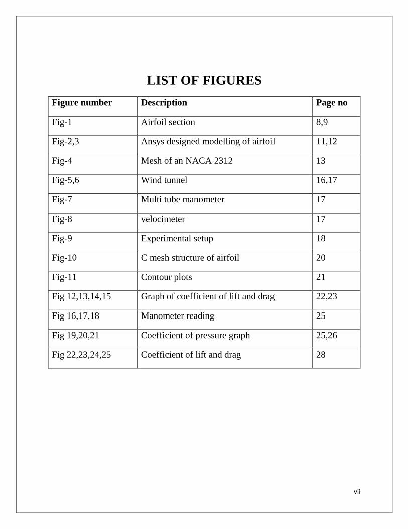
LIST OF FIGURES

Figure number Description Page no

Fig-1 Airfoil section 8,9

Fig-2,3 Ansys designed modelling of airfoil 11,12

Fig-4 Mesh of an NACA 2312 13

Fig-5,6 Wind tunnel 16,17

Fig-7 Multi tube manometer 17

Fig-8 velocimeter 17

Fig-9 Experimental setup 18

Fig-10 C mesh structure of airfoil 20

Fig-11 Contour plots 21

Fig 12,13,14,15 Graph of coefficient of lift and drag 22,23

Fig 16,17,18 Manometer reading 25

Fig 19,20,21 Coefficient of pressure graph 25,26

Fig 22,23,24,25 Coefficient of lift and drag 28

viii

NOMENCLATURE

l= span

c= chord length (m)

= angle of attack

D= Drag Force

L= Lift Force

M= Moment

U= Free Stream Velocity

= Air density

= Dynamic viscosity (Ns/m2)

P= Free stream pressure (Pa)

p= local pressure (Pa)

Re= Reynolds no (Uc/)

Cp= pressure coefficient ((p-p)/ (0.5U2))

Cl= lift coefficient ( L/(0.5U2Cl))

Cd= drag coefficient (D/(0.5U2Cd))

NACA-National advisory committee of aeronautics

Cfd- computational fluid dynamics

CHAPTER 1

INTRODUCTION

1.1 Looking to nature In the past days, when human being was yet residing in the part of creation, the main method for

velocity was his legs. Subsequently, we have established faster and more plentiful methods for voyaging,

most recent comprising the air conveyance. Since, its innovation planes have been adopting more fame

as it is the quickest method of conveyance accessible. It has additionally picked up fame as a war

machine since World War II. This prominence of air transport has prompted numerous innovations and

exploration to grow quicker and more conservative planes. This work is an attempt to adjudicate how

we can deduce most extreme execution from an aerofoil segment.

An aerofoil is a cross section of wing of the aircraft. Its fundamental occupation is to give lift to a

plane amid departure keeping in mind of trajectory. Yet, it has a component of resultant force called

pressure –form drag which restricts the movement of the plane. The measure of coefficient of lift

and its force required by an aircraft relies on upon configuration and assembly of various parts to

the concerned aircraft. Heavier one accommodate more lift while lighter oblige less compared to

heavier ones. Accordingly, contingent on the utilization of plane, aerofoil area is resolved. Lift

however exert additional prediction to the uplift raising speed of the aircraft, which in turns

depends on upon the plane with respect to flat speed. Hence, the coefficient of lift and coefficient

of pressure is the deciding factor to ascertain how the lift respond as per the velocity and various

parameters.

Aircraft wings which are horizontal and vertical stabilizers, helicopter rotor blades, propellers, fans,

compressors turbines all have aerofoil designs. Even sails, swimming and flying creatures employ

aerofoils. An airfoil-shaped ribs is sufficient to get down the force on an automotive parts or other

motor conveying device so to improve the adhesive friction that is traction.

A wing following the laminar flow has a greatest affinity of thickness in the centre part of camber

line. It demonstrates a negative weight inclination along the flow has the same impact as decreasing

the rate when we dissect the Navier–Stokes mathematical statements in the straight administration.

So on the off chance that we keep up greatest camber in the centre, a laminar flow over a bigger

rate of the wing at a higher velocity can be attained to. Nonetheless, with particles on the wing, this

does not work. Since such a wing slows down more effectively than others.

1

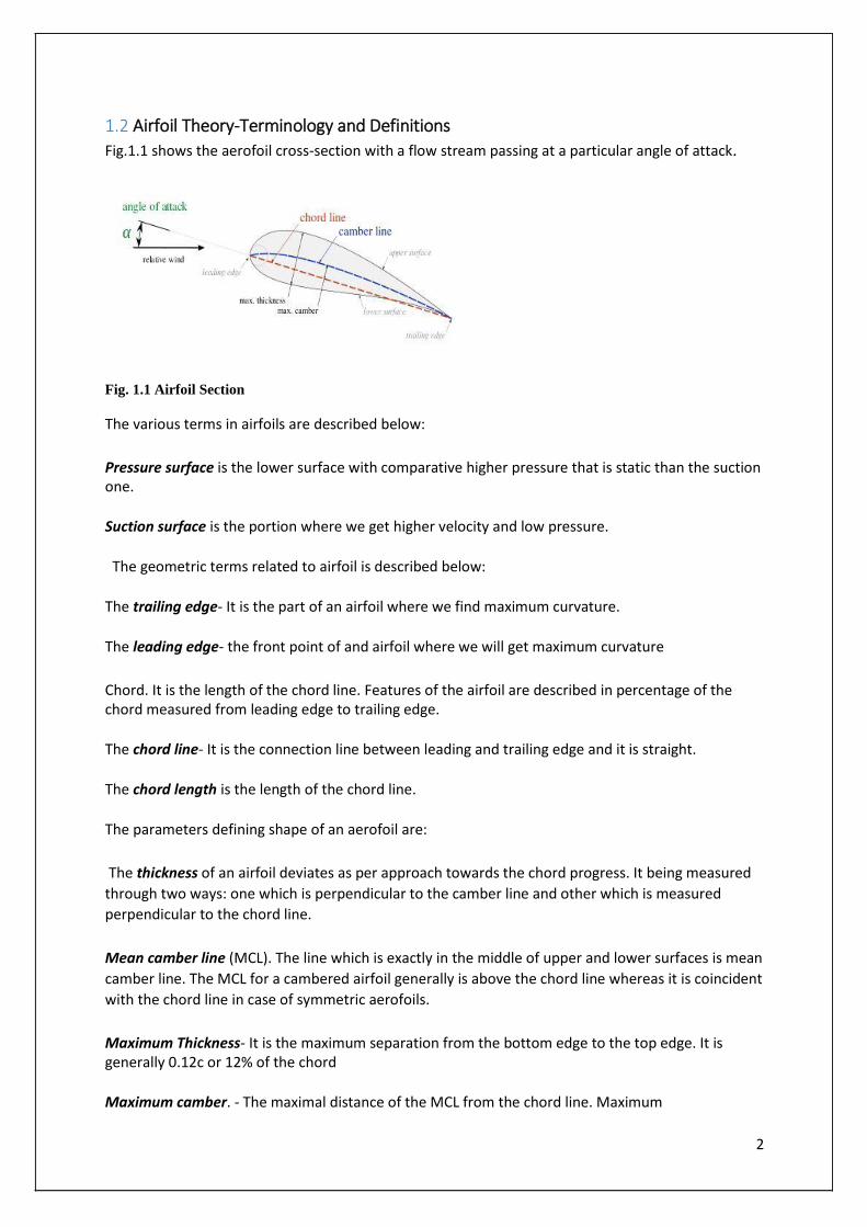
1.2 Airfoil Theory-Terminology and Definitions Fig.1.1 shows the aerofoil cross-section with a flow stream passing at a particular angle of attack. Fig. 1.1 Airfoil Section The various terms in airfoils are described below:

Pressure surface is the lower surface with comparative higher pressure that is static than the suction one.

Suction surface is the portion where we get higher velocity and low pressure.

The geometric terms related to airfoil is described below:

The trailing edge- It is the part of an airfoil where we find maximum curvature.

The leading edge- the front point of and airfoil where we will get maximum curvature

Chord. It is the length of the chord line. Features of the airfoil are described in percentage of the chord measured from leading edge to trailing edge.

The chord line- It is the connection line between leading and trailing edge and it is straight.

The chord length is the length of the chord line.

The parameters defining shape of an aerofoil are:

The thickness of an airfoil deviates as per approach towards the chord progress. It being measured

through two ways: one which is perpendicular to the camber line and other which is measured

perpendicular to the chord line.

Mean camber line (MCL). The line which is exactly in the middle of upper and lower surfaces is mean

camber line. The MCL for a cambered airfoil generally is above the chord line whereas it is coincident

with the chord line in case of symmetric aerofoils.

Maximum Thickness- It is the maximum separation from the bottom edge to the top edge. It is generally 0.12c or 12% of the chord

Maximum camber. - The maximal distance of the MCL from the chord line. Maximum

2

Camber is generally expressed as a % or fraction of the chord.

Leading Edge Radius- The radius of a circle that produces the leading edge curvature.

Stalling speed is the slowest speed at which aircraft can fly in straight and level flight. It is defined in terms of the maximum lift coefficient as follows:-

L=

1

v2SCl or v=√ 2

where L=W (1.1)

2

Therefore, higher the lift, lesser the stalling speed.

Angle of attack is defined as the angle between the chord line and the relative wind or flight path.

Total aerodynamic force (TAF) is the total force on the airfoil produced by the airfoil shape and relative wind. Lift is the perpendicular component of TAF to the relative wind or flight path. Drag is the parallel component of TAF to the relative wind or flight path. Flap is an artificial high lift providing device attached to the aerofoil section at trailing edge.

When flap is deflected downwards, the lift coefficient increases due to increase in camber of

aerofoil sections.

1.3 Airfoil profiles designation The NACA aerofoils are aerofoil shapes for air ship wings which are created by the National

Advisory Committee for Aeronautics (NACA). The state of the NACA aerofoils is depicted regarding

arrangement of digits taking after "NACA". The numerical code can be gone into mathematical

statements of aerofoil to produce the cross-area of the aerofoil and compute its properties. The

NACA aerofoil arrangement, the 4-digit, 5-digit, and adjusted 4-/5-digit, were created utilizing

scientific comparisons that portray the camber of the mean- line (geometric centreline) of the

aerofoil area and additionally the segment's thickness conveyance along the length. Later, including

the 6-Series, confused shapes were inferred utilizing hypothetical techniques. Prior to the National

Advisory Committee for Aeronautics (NACA) added to these arrangements, aerofoil configuration

was somewhat discretionary outlines aside from past involvement with known shapes and

experimentation with adjustments to those shapes. Distinctive NACA aerofoil profiles are

demonstrated as underneath:

1.3.1 Four-digit series

The NACA four-digit wing sections define the profile by:

First digit provides maximum camber which is in percentage of the total chord length.

Second digit provides the distance of maximum camber from leading edge in tens of percentage of the chord.

Last two digits describe maximum thickness of the airfoil as percentage of the chord.

3

For instance, the NACA 2312 aerofoil has a greatest camber of 2% found 40% (0.4 chord) from the

leading edge with a most extreme thickness of 12% of the chord. Four-digit arrangement aerofoils as

a matter of course have most extreme thickness at 30% of the chord (0.3 chords) from the main

edge.

The NACA 0015 aerofoil is symmetrical aerofoil0, the 00 indicating that it has no camber. The 15 indicates that the airfoil has a 15% thickness to chord length ratio.

1.3.2 five-digit series

The NACA five-digit series describes more complex airfoil shapes:

The first digit is multiplied by 0.15, gives the planned hypothetical ideal lift coefficient.

The second digit is multiplied by 5, the relative position, as a rate, of the purpose of greatest camber along the chord.

The third digit shows whether the camber is straightforward (0) or reflex (1).

.The fourth and fifth digits gives the greatest thickness of the airfoil (as a rate of the harmony), the same as 4-digit NACA profiles.

For example, the NACA 23112 profile- an airfoil with design lift coefficient of 0.3 (0.15*2), the point

of maximum camber at 15% chord (5*3), reflex camber (1), and maximum thickness of 12% of chord

length (12).

The camber-line is defined in two sections:

Where the chord wise location x and the ordinate y have been normalized by the chord. The

constant m is chosen so that the maximum camber occurs at x=p; for example, for the 230 camber-

line, p= 0.15 and m=0.2025. Finally, constant k1 is determined to provide the desired lift coefficient.

For a 230 camber-line profile (the first 3 numbers in the 5 digit series) k1 = 15.957 is used.

The NACA 6, 7 arrangements were intended to highlight some aerodynamic properties. Case in

point, NACA 653-421 is a 6-arrangement aerofoil in which the base pressure's position in tenths

chord is demonstrated by the second digit (here, at the 50% chord area), the subscript 3 implies that

the drag coefficient is close to its base worth at lift coefficients of 0.3 above and beneath the outline

lift coefficient. The following digit demonstrates the lift coefficient in tenths (here, 0.4) and the last

two digits give the greatest thickness in rate of chord (here, 21% of chord).

4

1.4 Types of flow on Airfoils

Laminar stream is portrayed by layers, or laminas, of air moving at the same rate and in the same

course. No fluid is traded between the laminas and the stream require not be in a straight line. The

closer the laminas are to the airfoil surface the slower they move. For a perfect liquid the stream

takes after the bended surface easily, in laminas. In turbulent stream, the streamlines or stream

examples are muddled and there is a exchange of liquid between these ranges. Momentum is

likewise traded such that slow moving liquid particles accelerate and quick moving particles

surrender their energy to the slower moving particles and ease off themselves. All or about all

liquid stream shows some level of turbulence.

The Reynolds number is an essential worth for the conduct of the stream, and particularly the limit

layer. Streams with the same Reynolds number carry on comparative. This number can be computed

by the accurate formula. If medium accuracy is sufficient, the Reynolds number can be

approximately calculated by the equation given below:

Re= v × l ×70000

Where: “v” is flight speed

“L” is chord length in m.

70000 constant value for air (s/m2).

The Reynolds number is in light of a length, which is typically the chord length of an airfoil (in two

measurements) or the chord length of a wing. Since the chord length of a wing may fluctuate

from root to tip, a mean aerodynamic chord length is utilized to characterize the Reynolds

number for a wing.

Different sorts of stream incorporate subsonic (Mach No M < 0.1), transonic and supersonic

streams over the aerofoils. Correspondingly the fluid may b considered as compressible or

incompressible or inviscid.

1.5 Literature review This section explains some previous literature on aerofoil sections and their analysis procedure.

Rana et al. [1] studied the flutter characteristics of an airfoil in a 2-D subsonic flow by using RANS based CFD solver with a structural code in time domain.

Gultop[2]contemplated the effect of viewpoint degree on Airfoil execution. The explanation behind this study was to center the swell conditions not to be kept up all through wind passage tests.

Goel[3]formulated a technique for advancement of Turbine Airfoil utilizing Quansi – 3D examination

codes. He understood the intricacy of 3D demonstrating by displaying numerous 2D air foil segments

5

and joining their figure in spiral bearing utilizing second and first order polynomials that prompts no harshness in the radial direction.

Arvind [4] looked into on NACA 4412 aerofoil and investigated its profile for thought of a plane wing .The NACA 4412 aerofoil was made utilizing CATIA V5 And examination was completed utilizing

business code ANSYS 13.0 FLUENT at a rate of 340.29 m/sec for angle of attacks of 0˚, 6, 12 and

16˚. k-ε turbulence model was accepted for Airflow. Changes of static weight and element weight

are plotted in type of filled shape.

Fazil and Jayakumar [5] presumed that in spite of the way that it is less requesting to model and

make an aerofoil profile in CAD environment using camber billow of concentrates, after the

making of vane profile it is extraordinarily troublesome to change the condition of profile for

dismemberment or change reason by using surge of core inter.

Kevadiya [6] concentrated on the NACA 4412 aerofoil profile and remembered its significance for

examination of wind turbine edge. Geometry of the aerofoil is made using GAMBIT 2.4.6.

Additionally CFD examination is done using FLUENT 6.3.26 at distinctive methodologies from 0˚ to

12˚.

Guilmineau et al. [7] talked about the processing of the time-mean, turbulent, two-dimensional

incompressible thick stream past an airfoil at settled rate. Another physically reliable technique is

exhibited for the reproduction of speed fluxes which emerge from discrete mathematical statements

for the mass and energy equalization. This conclusion strategy for fluxes makes conceivable the

utilization of a cell-focused network in which speed and pressure questions have the same location,

while going around the event of spurious pressure modes.

Kunz and Kroo [8] advanced aerofoils at ultra-low Reynolds numbers. These examinations are done

to comprehend the aerodynamic issues identified with the low speed and miniaturized scale air

vehicle outline and execution. The enhancement strategy utilized is in view of concurrent pseudo-

time venturing in which stationary states are acquired by fathoming the preconditioned pseudo-

stationary arrangement of comparisons.

N. Ahmed et al. [9] contemplated the numerical reproduction of stream past aerofoils is vital in the

flight optimized outline of air ship wings and turbo-hardware parts. These lifting gadgets

regularlyachieve ideal execution at the state of onset of partition. Hence, division phenomena must

be incorporated if the examination is gone for pragmatic applications. Thus, in the present study,

numerical recreation of relentless stream in a straight course of NACA 0012 aerofoils is expert with

control volume approach.

Mittal et al. [10] performed the computational examination for two-dimensional stream past

stationary NACA 0012 aerofoil is completed with dynamically expanding and diminishing

approaches. The incompressible, Reynolds averaged Navier–Stokes mathematical statements in

conjunction with the Baldwin–Lomax model, for turbulence conclusion, are explained utilizing

settled limited element formulations.

Several experimental studies were also conducted to understand the dynamic behaviour and flow characteristics of aerofoil sections.

6

Genc et al [11] conducted experiments on NACA 2415 aerofoil by varying angle of attack from -120

to 200 at low Reynolds number flight regime (0.5x105 to 3x105). Using pitot static tube, scan valve

and pressure transducer, the pressure distribution over aerofoil was measured. Lift, drag and pitching moment were obtained by 3-component load cell system. Hot wire anemometer and oil flow visualization was used to photograph surface flow patterns.

1.6 OBJECTIVE AND SCOPE OF PRESENT WORK The objective of this project is to understand the phenomena of the uniqueness of aerofoil shape.

Aerofoil shapes are employed in aircraft sectors as well as in automobile and production sectors e.g.

wind turbines, wing of an automobile etc. It can generate lift as well as downforce when used in a

specific manner. So it is quite important to decode the phenomena behind its shape and the process

by which it produces necessary lift and downforce.

The main objective is to study the design process of various aerofoils and their flow simulation to understand how they work. But, the following are the essential objectives of the work:

Obtain the pressure distribution, lift and drag coefficients on the given aerofoil profile using Ansys at various AOA in viscous domain.

Experimental investigation on the airfoil at various AOA and free stream velocity. AOA varies from 0 to 20 degree and free stream velocity ranges from 12 to 14.5m/s

To compare the results obtained by CFD analysis, correlations developed with the

corresponding experimental one.

7

CHAPTER 2

MATHEMATICAL MODELLING AND NUMERICAL SIMULATION This chapter explains the method of generation of airfoils, fluid analysis and Panel method used for 2-D airfoils.

2.1 Airfoil Profile Generation Airfoil cross-sections are asymmetric in nature, where the shear center and center of flexure are not coincident. Often it requires an integration of geometry modeler, mesh generator and CFD solver. The asymmetric NACA airfoil series is controlled by its digits.

The NACA four-digit wing sections define the profile by: The first digit specifies the maximum camber (m) in percentage of the chord (airfoil length), the

second indicates the position of the maximum camber (p) in tenths of chord, and the last two

numbers provide the maximum thickness (t) of the airfoil in percentage of chord. For example, the

NACA 2312 airfoil has a maximum thickness of 12% with a camber of 2% located 30% back from the

airfoil leading edge (or 0.4c). Utilizing these m, p, and t values, we can compute the coordinates for

an entire airfoil using the following relationships:

1. Pick values of x from 0 to the maximum chord c.

2. Compute the mean camber line coordinates by plugging the values of m and p into the

Following equations for each of the x coordinates.

(2.1) Where,

x = coordinates along the length of the airfoil, from 0 to c (which stands for chord, or

length) y = coordinates above and below the line extending along the length of the airfoil

8

t = maximum airfoil thickness in tenths of chord (i.e. a 15% thick airfoil would be 0.15) m = maximum camber in tenths of the chord p =position of the maximum camber along the chord in tenths of chord

3. Calculate the thickness distribution above (+) and below (-) the mean line by plugging the Value of t into the following equation for each of the x coordinates

(2.2) 4. Determine the final coordinates for the airfoil upper surface (xU, yU) and lower surface (xL, yL) Using the following relationships

Upper surface xu= xc –ytsin(ɵ) yu= yc –ytcos(ɵ)

Lower surface xl= xc +ytsin(ɵ) yl= yc –ytcos(ɵ) (2.3)

Where tan θ= (2m/p) (p-x), 0≤x≤p

= (2m/ (1-p)2)(p-x) , p≤ x ≤ 1 (2.4) The most obvious way to plot the airfoil is to iterate through equally spaced values of x calculating the upper and lower surface coordinates. The points are more widely spaced around the leading edge where the curvature is greatest. To group the points at the ends of the airfoil sections cosine spacing is used with uniform increments of β

(2.5) 2.2 NUMERICAL SIMULATION

2.2.1 COMPUTATIONAL FLUID DYNAMICS AND ANALYSIS

CFD is a numerical technique used to recreate physical issues with utilization of fluid

comparisons. This methodology is utilized to research plan without making a physical model –

and can be an important to comprehend properties of new mechanical plans. By utilizing a

simulation as opposed to doing lab tries, one may get results faster. A vital thing in the utilization

of CFD is to comprehend the improvements in programming, and know the constraints. In spite

of the fact that the CFD programming uses surely understood representing comparisons, serious

disentanglements are made as far as matrix and representing geometries.

9

Flow over an airfoil is mathematically described by Navier-Stokes equation as follows:

+ (u.)u - .(u.p)= and .u=0, with as fluid density, being the body force.

2.2.2 METHODOLOGY

The process of the numerical simulation of fluid flow using the above equation generally involves four different steps and the details are given below.

(a) Problem identification

1. Setting the modelling ends

2. Placing the model to domain.

(b) Pre-working

1. Creating an airfoil model to represent the C-domain

2. Meshing configuration

(c) Solver

1. Demonstrating the physics

Representing the flow (e.g. turbulent, laminar etc.) Placing the appropriate boundary condition.

2. Using different numerical strategy to discretize the governing equations.

3. Checking the convergence by iterating the equation till precision achieved.

4. Figure out the Solution by Solver Setting.

Initialization Solution Control Monitoring Solution

(d) Post processing

1. Analysing the results

10

2. Graphical diagrams

3. Contour Details

2.2.2.1 PREPROCESSING In this first step all the pertinent data which determines the problem is initialised by the exploiter.

This comprises geometry, computational grid formation, significant models to be used, and the

number of Eulerian levels, the time footprint and the numerical outlines.

2.2.2.1.1 PREPARING THE GEOMETRY MODEL

Using Computational fluid dynamics, a graphical user interface model that represents an arrangement

to carry out the study has been built. Then, implication of the fluid flow physics to this computational

model, and the involvement of software outputs a prediction to the concept of fluid dynamics. NACA

airfoils geometries were acquired as co-ordinate vertices i.e. writings document and imported into the

ANSYS programming. Some minor conformities were made to this to right the geometry and make it

substantial as a CFD model. ANSYS is fundamental during the time spent doing the CFD

investigation: it creates the workplace where the item is reproduced. An imperative part in this is

making the cross section encompassing the article. This needs to be reached out in all bearings to get

the physical properties of the encompassing fluid – for this case moving air. The mesh and edges

should likewise be gathered keeping in mind the end goal to define the essential limit conditions

adequately.

Fig 2

Fig 3 2.2.2.1.2 MESHING Second and very pertinent step in computational analysis is setting up the mesh domain followed with

the modelling of geometry. The Navier-Stokes Equations are non-linear partial differential equations,

which focus on the whole fluid field as a continuum process. In order to ease the problem the

corresponding equations are modified as simple flows that have been directly figured out at very low

Reynolds numbers. The conversion and reduction can be made by using what is called discretization.

Developing of mesh involves discretizing or dispersing the geometry into the cells or elements at which

the variables will be calculated numerically. By using the Cartesian co-ordinate system, the fluid flow

governing equations i.e. momentum equation, continuity equation are being solved as of the

11

Discretization of domain proceed. The CFD analysis needs a spatial discretization scheme and time

marching scheme. Meshing divides the continuous process into finite number of units. More often

the domains are discretized by three different ways i.e. Finite element, Finite difference and Finite

volume method. Finite element method is based on dividing the fluid area into desired elements. In

finite element method the numerical solutions are obtained by integrating the corresponding shape

function and weighted factor in a set aside domain. Both structured and unstructured mesh being

solved perfectly and analytically. But the Finite Volume method discretize the domain into finite

number of volumes. Finite volume method solves the discretization equation in the center and

computes some specified variables. The values of fluid properties, such as pressure, density and

velocity that are present in the concerned equations to be solved are stored at the pivot of each

volume. The flux into the region is computed as the sum of the fluxes at the boundaries of the

concerned region. As the values of parameters are stored at nodes but not at boundaries this

method followed some interpolation at nodes. Mostly finite Volume method is desirable for

unstructured domain. Whereas finite Difference method is grounded on the estimation of Taylor's

series. This method is more suitable for regular domain.

For transient flow problems an earmark time level needs to be confirmed. To captivate the desired

features of fluid flow with in a domain, the time step should be sufficiently modest but not too

much small which may cause barren of computational power and time. Spacial and time

discretization are linked, apparent in the Courant number.

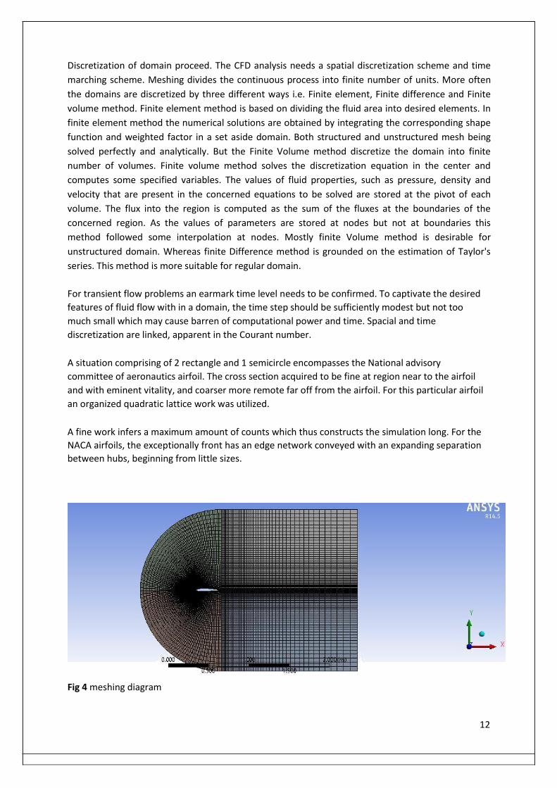
A situation comprising of 2 rectangle and 1 semicircle encompasses the National advisory

committee of aeronautics airfoil. The cross section acquired to be fine at region near to the airfoil

and with eminent vitality, and coarser more remote far off from the airfoil. For this particular airfoil

an organized quadratic lattice work was utilized.

A fine work infers a maximum amount of counts which thus constructs the simulation long. For the

NACA airfoils, the exceptionally front has an edge network conveyed with an expanding separation

between hubs, beginning from little sizes. Fig 4 meshing diagram

12

The aforementioned meshing structure has been accomplished by considering mapped meshing and applying various edge sizing criteria to carry out the task. While defining edge sizing no of division taken is 50 and bias factor been considered as 10. 2.2.2.1.3 Solver settings

The numerical strategy that CFD codes acquire is the finite volume method. The differential

transport equations are then followed by integration throughout each of the computational cell,

and subsequently Gauss and Leibnitz theorems are employed in this method. This comprises of

several models used for flow analysis, the starting and boundary situations, the number of

Eulerian levels, the holdings and properties of the materials, the physical and chemically

development implication. Ultimately, the corresponding algebraic equations is figured out by

iteration process and the corresponding centred values of the flow variables are calculated.

2.2.2.1.3.1

A large count of flows that came across in nature are known as a mixture of different phases.

Solidus, liquidness and gaseous are three physical phase of matter. But the construct of phase in

a polyphase flow rate system is implemented in a vast way. Subjected to multiphase fluid flow, a

phase point is elaborated as a peculiar class of material that has a definite certainty towards

inertial response and fundamental interaction with the fluid current and the potential field in

which it is plunged. Presently there are two accesses for the mathematical calculation of

multiphase flows: the personified Euler-Lagrange approach and the noted Euler-Euler approach. Overtures of Euler Lagrange

In Ansys Fluent, the Lagrangian concepts discretise the desired phase model following the Euler-

Lagrange approach. The fluid state is treated as a continuous nonspatial whole or extent or

succession in which no part or portion is distinct or distinguishable from adjacent parts by solving

the very known and popular Navier-Stokes equations, while the dispelled phase is solved by dogging

a large count of various particles, bubbles or droplets through the computed flow field. The

dispelled phase can exchange the momentum, mass, and energy within the fluid phase.

13

Overtures of Euler Euler

In the Euler-Euler approach, the different phases are addressed as a permeating continua. Since

the corresponding volume of a phase cannot be acquired by the other phases, the volume of

fraction concept is implemented in the scenario. However these particular constituent of of a

mixture that has been separated by a fractional process are assumed to be uninterrupted functions

of space and time whose corresponding sum is equal to one.

There are three different access path in Euler-Euler polyphase models i.e. the Eulerian model volume

of fluid (VOF) model, the mixture model. The VOF model is nothing but a surface-chasing technic

which is employed for a defined Eulerian mesh. It is expended for two or more non-miscible fluids

where the location of the concerned interface between the respective fluids are of paramount

interest. In the VOF model, a single characteristic arrangement of momentum equation is

apportioned by the fluids, and the fraction of volume towards each of the fluids in computational

cell is complied throughout the c-domain. Whereas the valuable mixture model is contrived for two

or more level of phases (fluid or particulate) and it figure out for the directed mixture momentum

equation and proposes relative velocities to depict the dispersed phases. But in the Eulerian model,

the phases are treated as permeating continua.

Setting up Fluent

The coordinates from the standardized national advisory committee of aeronautics were imported

and the geometries have been constructed in the modelling window and subsequently mesh been

spelt to the FLUENT, and the respective framework and surroundings attributes were set to the

concerned place. Launched the “Double precision" panel window and considered it as a

framework arguments, guaranteeing sufficient exactness. The FLUENT has pivot exactness as

default consideration, however towards these reproductions a precise arrangement is asked. The

remainders for the distinctive model variables constrained to turbulence zone were situated as 10

to 8 and the cycle upper limit check to 1000. The computer simulation procedure however

likewise to be stopped or quitted if the corresponding coefficient of lift (CL) or coefficient of

drag (CD) appeared to exhibit balanced out appropriately.

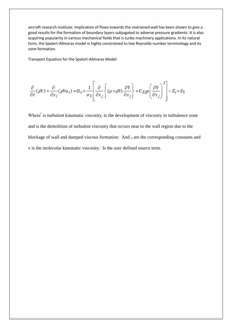
Model Spalart-Allmaras model

The Spalart-Allmaras model defines a single-equation model that resolves a transport equation of the designed modelled for the unavoidable kinematic viscosity that forms turbulence eddies. The Spalart-Allmaras model was formulated specifically for the applications of aero industries and

14

aircraft research institute. Implication of flows towards the restrained wall has been shown to give a

good results for the formation of boundary layers subjugated to adverse pressure gradients. It is also

acquiring popularity in various mechanical fields that is turbo machinery applications. In its natural

form, the Spalart-Allmaras model is highly constrained to low Reynolds number terminology and its

zone formation. Transport Equation for the Spalart-Allmaras Model

Where ̃ is turbulent kinematic viscosity, is the development of viscosity in turbulence zone

and is the demolition of turbulent viscosity that occurs near to the wall region due to the

blockage of wall and damped viscous formation. ̃ And 2 are the corresponding constants and

v is the molecular kinematic viscosity. ̃ Is the user defined source term.

3 Chapter 3 3.1 Experimentation General Experimental information useful for solving aerodynamics problems may be obtained in a number of

ways: from flight test, water tables, flying scale models, subsonic transonic, supersonic and hypersonic

wind tunnel. Each device has its own sphere of superiority. The nations of the world support research, of

which wind tunnel testing is a major item, according to their desired and abilities. For the past some

decades now, wind tunnels have been a pivot component in scientific research area followed by

hierarchical fields. Experimenting with the prototype of Mercedes Benz, Bugatti Veyron, various superfast

cars followed by experimentation of air wings, complete aircraft, various weather patterns that is

research on rain droplet, icing have been caused much ease because of its evolution. The structure of

birds plays a vital role in aerodynamics to proposed a research on various wings that should be light

weighted to identify the difference between nature and artificial. In the field of race the selective

information accumulated from this research testing can mean the conclusion between winning and losing

a race. The idea of simulating weather response also providing vital information about the reliability

towards building stability and safety. This has turned into very pertinent when buildings designs come to

the picture. Valuable and appropriate data considering bird maneuvering has also been gathered based

on wind tunnel testing. Researchers have done lot of experimentation with a hell lot of birds and

collected enormously useful information regarding loss of mass with respect to time during maneuvering,

respiratory data linkage, and in kinematics of flight. Wind tunnels have a hierarchical of usage in the

current world today.

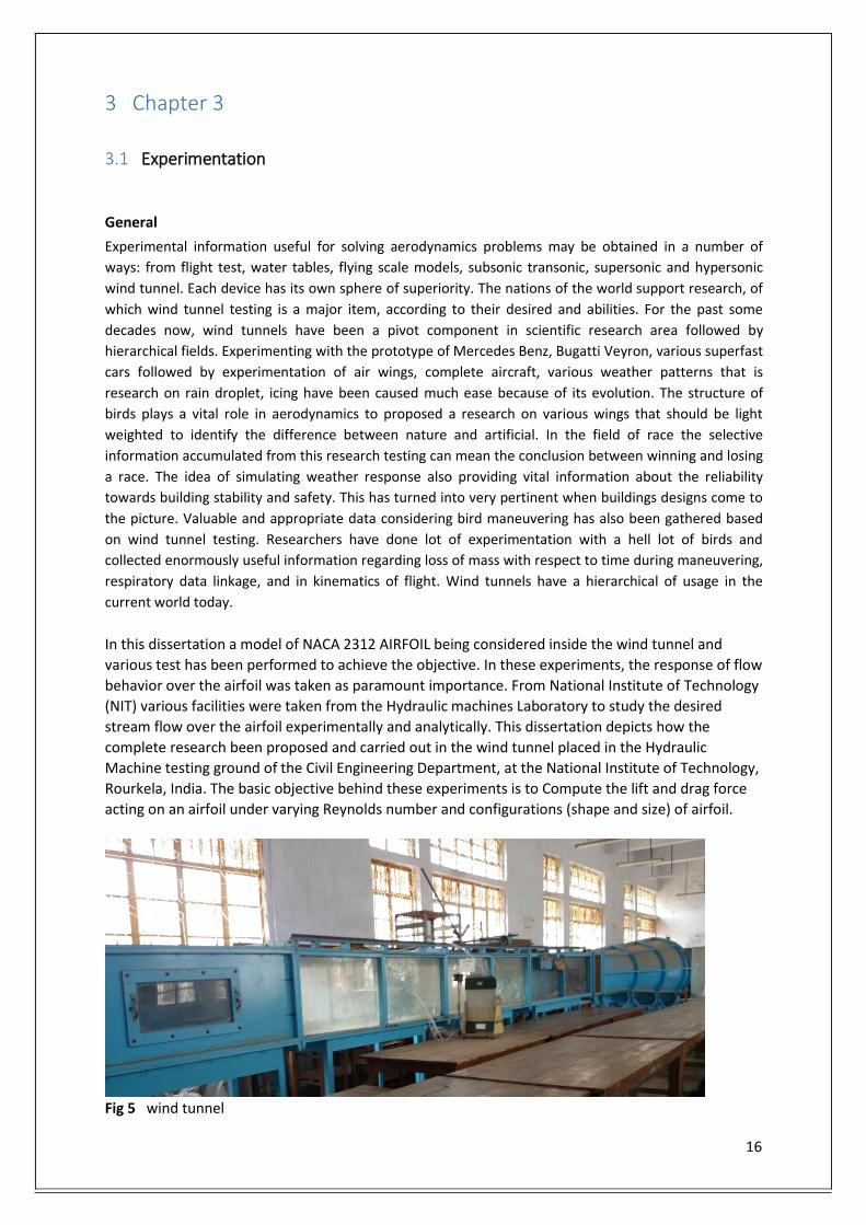
In this dissertation a model of NACA 2312 AIRFOIL being considered inside the wind tunnel and

various test has been performed to achieve the objective. In these experiments, the response of flow

behavior over the airfoil was taken as paramount importance. From National Institute of Technology

(NIT) various facilities were taken from the Hydraulic machines Laboratory to study the desired

stream flow over the airfoil experimentally and analytically. This dissertation depicts how the

complete research been proposed and carried out in the wind tunnel placed in the Hydraulic

Machine testing ground of the Civil Engineering Department, at the National Institute of Technology,

Rourkela, India. The basic objective behind these experiments is to Compute the lift and drag force

acting on an airfoil under varying Reynolds number and configurations (shape and size) of airfoil. Fig 5 wind tunnel

16

3.2 SPECIFICATION OF WINDTUNNEL The wind tunnel used in this project is a subsonic wind tunnel located in the Hydraulic Machines Laboratory of National Institute of Technology, Rourkela, and Odisha. This wind tunnel is an open circuit wind tunnel whose specifications of dimensions are tabulated as follows;

COMPONENTS LENGTH(m) INLET(m) OUTLET(m)

Converged Effuser 1.3 2.1×2.1 2.1×2.1

Pivot Test section 8 0.6×0.6 0.6×0.6

Diverged diffuser 5 0.6 1.3

Fig 6

3.3 EQUIPMENTS USED Multitube manometer

Very frequently it is necessary to measure large no of

pressures simultaneously.normally the accuracy needed

does not require precision equipment and it is sufficient to

mount a large number of glass tubes on a lined

plate,forming what is called a multi tube manometer.for

low speed work the manometer must be lowered until it is

from 30 to 45 deg with the horizontal in order to get

useful fluid heights.cluster plugs were being installed over

the multitube manometer for the better connection

Fig 7

17

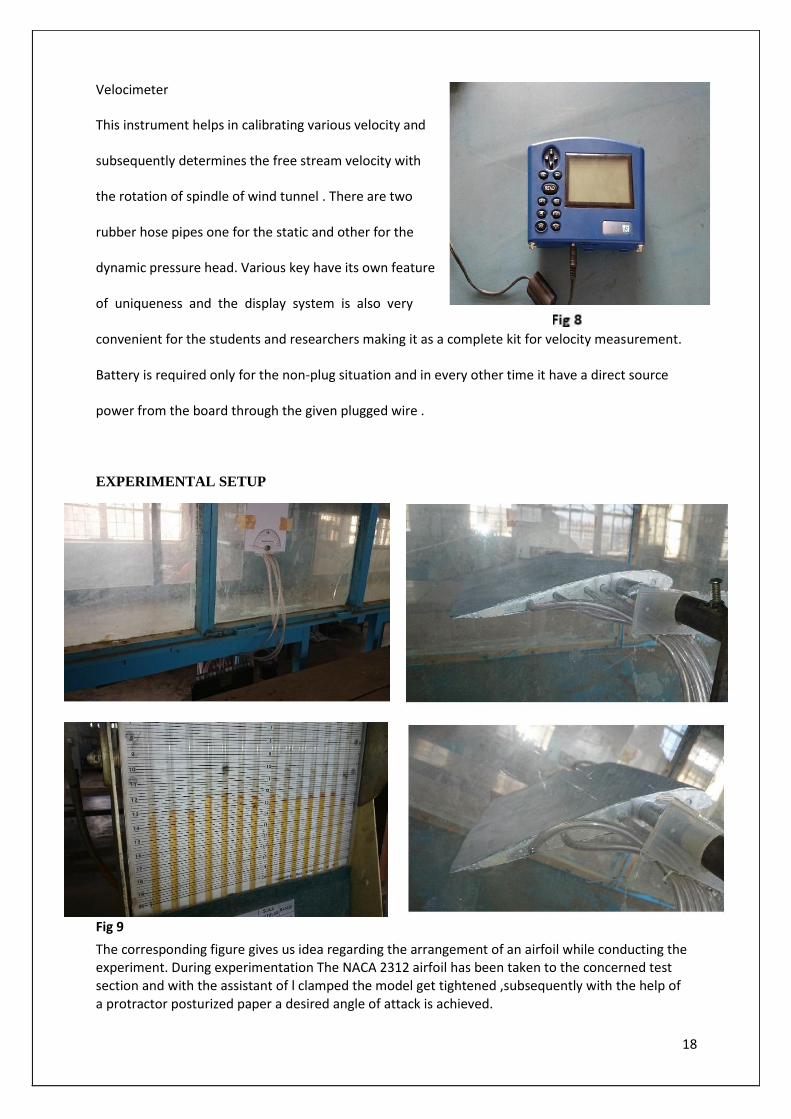
Velocimeter This instrument helps in calibrating various velocity and

subsequently determines the free stream velocity with

the rotation of spindle of wind tunnel . There are two

rubber hose pipes one for the static and other for the

dynamic pressure head. Various key have its own feature

of uniqueness and the display system is also very

convenient for the students and researchers making it as a complete kit for velocity measurement. Battery is required only for the non-plug situation and in every other time it have a direct source

power from the board through the given plugged wire . EXPERIMENTAL SETUP Fig 9 The corresponding figure gives us idea regarding the arrangement of an airfoil while conducting the experiment. During experimentation The NACA 2312 airfoil has been taken to the concerned test section and with the assistant of l clamped the model get tightened ,subsequently with the help of a protractor posturized paper a desired angle of attack is achieved.

18

3.4 Procedure

The airfoil is placed inside the test section having ‘closed ends’ arrangement thus airflow is only flow across the curved surfaces of the airfoil. This condition comes over the wing tip vortices or drag caused by wing tips. By the way two dimensional flow is observed around airfoil. One of the best advantage of the arrangement is ‘infinite span’.

Pressure tapings are placed along the upper and lower surfaces of the airfoil.. These

tapings are connected to a set of numbered small pipe connectors on a plate which are

located next to the airfoil.

A set of larger bore pipes connects the numbered pipe connectors to the multitube manometer.

At the inlet part of the duct, just above the airfoil there is an extra pressure

tapping which is placed to measure static pressure upstream of the airfoil

The performance of an airfoil can be observed from lift curves. In this experiment we want to measure the performance of the wing by using NACA 2312 airfoil. We can measure performance of the wing by measuring the pressures on the two surfaces of the airfoil, relative to local air pressure.

one manometer tube was leave behind and the common manometer connection open to the atmosphere

Arranged the locking screw and set the airfoil to zero angle

Connected the static pressure at the top of the wind tunnel to the last manometer tube then measure the pressure

Recorded the all manometer readings for the tapping for the airfoil. Increased angle of attack positively 5 degree in each step up to 25. Coefficient of pressure is calculated using

Cp p

i

p

1 U 2

2

19

Chapter 4

Results and discourse 4.1. Fluent outcomes

This figure highlighting the mesh of an airfoil with c mesh domain. The mapped meshing is

created on entire c-domain. The cross section is developed to be fine at areas near to the

airfoil and coarser more remote far placed irrespective to the position of airfoil. For this

particular airfoil a quadratic formation of an element was utilized. The mesh has to be smooth

and fine also in some regions away from the airfoil. Various edge sizing has been adopted to

accomplish the task.

Fig 10 meshing details 4.2 PRESSURE AND VELOCITY DISTRIBUTION

The NACA 2312 airfoil is tested against a various angle of attacks such as 5, 10, and 15 degree. The

pressure contour and velocity vectors are plotted and shown in figures (Fig. 11). The velocity vector

gives the clear picture of the velocity distribution and the pressure contour gives clear picture of static

pressure over an airfoil. The pressure coefficient over an airfoil is also plotted with help of Fluent and

is compared with the experimentation data to give a clear indication of stalling, and various response

of flow over an airfoil.

FIG 11 contour plots

The above diagrams have its own significance and also the colour tone have its own meaning.the

above diagram are contour diagram for an angle of attack 5 degree,10 degree and 15 degree which

says that how lift is generated and how bernoullis law come to the play.exactly when flow occurs

over an airfoil after due course of tim as flow keep on cross through an intial starting vortex get

formed behind the airfoil and to counteract that developed anticlockwise vortex a velocity vector

get into the process due to conservation of angular momentum and subsequently that velocity get

added with the main stream velocity and give rise to higher velocity over the upper surfgace of an

airfoil and lower velocity under the lower surface which consequently as per bernoullis results in

higher pressure in the lower side and higher pressure over the top surface. FOR 12M/S AND AT DIFFERENT ANGLE OF ATTACK

Cl [-]

Cd [-]

3 0.2

2.5

0.15

2

0.1

1.5

0.05

1

0.5

0

0 0 5 10 15 20 25

0 5 10 15 20 25 21

+

FOR 13 M/S AND AT DIFFERENT ANGLE OF ATTACK

Cl [-] Cd [-]

3

0.18

0.16

2.5 0.14

0.12

2

0.1

1.5 0.08

0.06

1

0.04

0.5 0.02

0

0 0 5 10 15 20 25

0 5 10 15 20 25

FOR 14.5 M/S AND VARIOUS ANGLE OF ATTACK

Cd [-]

Cl [-]

3 0.2

2.5 0.15

2

0.1

1.5

1 0.05

0.5

0

0

0 5 10 15 20 25

0 5 10 15 20 25

The above fig 13, 14 and 15 reflects how the coefficient of lift and coefficient of drag varies with

respect to the angle of attack. The above graph depicts that coefficient of lift increase as per the

increment of angle of attack whereas coefficient of drag show some gradual response. Coefficient of

drag increases slowly till angle of attack 10 degree and after that it show spontaneous and upwards

increment

22

4.3 EXPERIMENT RESULTS Readings of an airfoil model tested in wind tunnel

The readings have been proposed over an NACA 2312 airfoil model inside the test section

of a wind tunnel at different air velocity 12m/s,13m/s,14.5m/s.Manometer reading at

12m/s,13m/s and 14.5 m/s

Table 1 manometer reading at 12m/s TABLE 2 manometer reading at 13m/s

Table 3 manometer reading at 14.5m/s

23

Coefficient of pressure

2.00000

0.00000 0 0.2 0.4 0.6 0.8 1 1.2

-2.00000

-4.00000

-6.00000

-8.00000

-10.00000

-12.00000

cp at 0 cp at 5 cp at 10 cp at 15

Fig 19 coefficient of pressure against angle of attack

COEFFICIENT OF LIFT FOR 13M/S AND 14.5 M/S AGAINST VARIOUS ANGLE OF ATTACK

Coefficient of pressure

2.00000

0.00000 0 0.2 0.4 0.6 0.8 1 1.2

-2.00000

-4.00000

-6.00000

-8.00000

-10.00000

-12.00000

cp at 0 cp at 5 cp at 10 cp at 15

Fig 20 coefficient of pressure against angle of attack for 13m/s

The above figure demonstrates that how dimensionless number that is coefficient of pressure

describing the pressure variation throughout the flow zone. Every point in the concerned graph has

its own unique pressure coefficient data. Typically the distribution of this graph indicates that

negative numbers are maximum on the graph as per the top surface response towards the flow

which lies farther under zero and consequently be the top lineage on the graph.

24

Chart Title

2.00000

0.00000 0 0.2 0.4 0.6 0.8 1 1.2

-2.00000

-4.00000

-6.00000

-8.00000

-10.00000

-12.00000

cp at 0 cp at 5 cp at 10 cp at 15

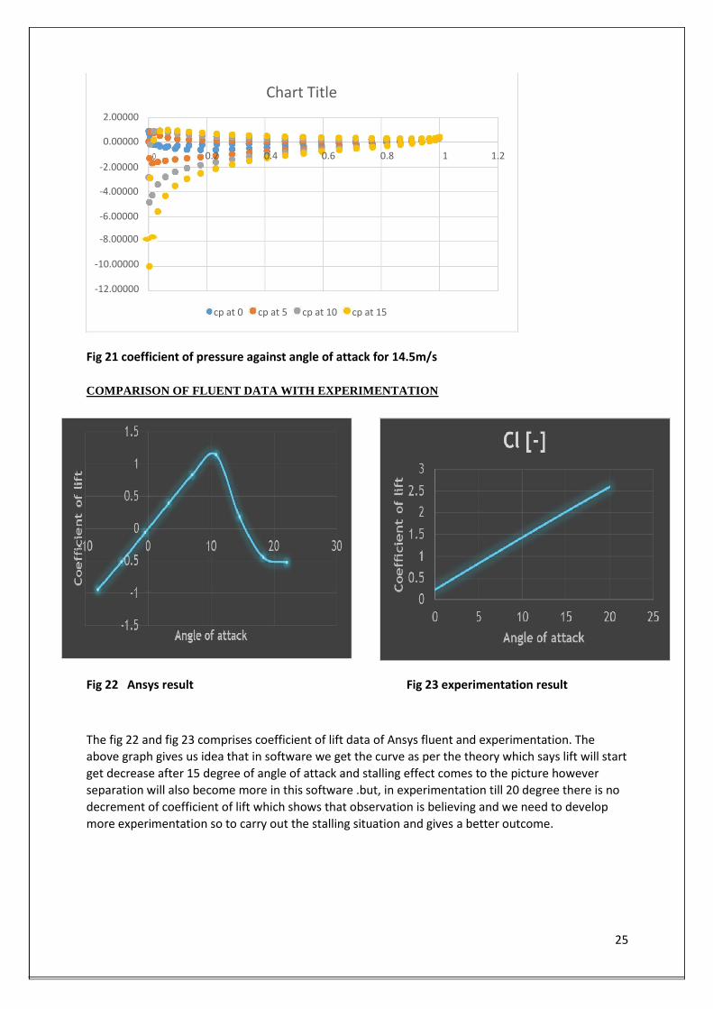
Fig 21 coefficient of pressure against angle of attack for 14.5m/s

COMPARISON OF FLUENT DATA WITH EXPERIMENTATION Fig 22 Ansys result Fig 23 experimentation result The fig 22 and fig 23 comprises coefficient of lift data of Ansys fluent and experimentation. The

above graph gives us idea that in software we get the curve as per the theory which says lift will start

get decrease after 15 degree of angle of attack and stalling effect comes to the picture however

separation will also become more in this software .but, in experimentation till 20 degree there is no

decrement of coefficient of lift which shows that observation is believing and we need to develop

more experimentation so to carry out the stalling situation and gives a better outcome.

25

Chapter 5 5.1 CONCLUSION

1. Coefficient of lift will be higher at an angle of 15 degree.

2. As the angle of attack increase the amount of lift created by the airfoil also increases

3. A lowering of pressure on the upper surface results in developing pressure gradient.

4. Coefficient of pressure show better results at 14.5 m/s

5. After comparing from the experimental data conclusion arise that stalling effect will

occur after 20 degree angle of attack.

5.2 Future scope

• Improve the modern airplane • New configuration • New rules and requirement

26

REFERENCES

• M.Kevadiya (2013)” CFD Analysis of Pressure Coefficient for NACA 4412” International

Journal of Engineering Trends and Technology ISSN/EISSN: 22315381 Volume: 4 Issue: 5

Pages: 2041-2043, 2013

• A.Zanotti, G. Gibertini, D. Grassi, and D. Spreafico, (2013)” Wake Measurements behind

an Oscillating Aerofoil in Dynamic Stall Conditions”.

• A.Zanotti and G. Gibertini, (2012) “Experimental investigation of the dynamic stall

phenomenon on a NACA 23012 oscillating aerofoil,” Proceedings of the Institution of

Mechanical Engineers, Part G: Journal of Aerospace Engineering.

• M.Arvind “CFD ANALYSIS OF STATIC PRESSURE AND DYNAMIC PRESSURE FOR NACA

4412” International Journal of Engineering Trends and Technology ISSN/EISSN: 22315381

Volume: 4 Issue: 8 Pages: 3258-3265,(2010)

• D.Rana, S.Patel, AK.Onkar and M.Manjuprasad, “Time domain simulation of airfoil flutter

using fluid structure coupling through FEM based CFD solver”, Symposium of Apllied

Aerodynamics and Design of Aerospace vehicle, SAROD20111, Nov 16-18 2009,

Bangalore

• S.Goel (2008) “ Turbine Airfoil Optimization Using Quasi-3D Analysis Codes.”

International Journal of Aerospace Engineering ISSN/EISSN: 16875974 16875974

Volume: 2009, 2008

• Kunz, P. J., Kroo, I.,Analysis, “design and testing of airfoils for use at ultra-low Reynolds

numbers, Proceedings of the Conference on Fised, Flapping and Rotary Vehicles at very

Low Reynolds Numbers”, edited by T. J. Mueller, Univ. of Notre Dame, Notre Dame, IN,

pp.349-372, 2000.

• Selig, M. S. and McGranahan, (2004) “Wind Tunnel Aerodynamic Tests of Six Aerofoils

for Use on Small Wind Turbines,”ASME Journal of Solar Energy Engineering, Vol. 126,

November, pp. 986–1001.

• J.W. Chang, (2004) “Near-wake characteristics of an oscillating NACA 4412 aerofoil,”

Journal of Aircraft, vol. 41, pp. 1240–1243.

• J. F. Manwell, J. G. McGowan, and A. L. Rogers, (2002) Wind Energy Explained, Wiley,

Amherst, Mass,USA, 1st edition.

• S. Mittal and P. Saxena; “Hysteresis in flow past a NACA 0012 airfoil”. Comput. Methods

Appl. Mech. Engrg. 191 2179– 2189, 2002

• T. Ackermann and L. S¨oder, “Wind energy technology and current status: a review,”

Renewable and Sustainable Energy “Reviews, vol. 4, no. 4, pp. 315–374, 2000.

• M.R. Ahmed, Y. Kohama,(1999) “Experimental investigation on the aerodynamic

characteristics of a tandem wing configuration inclose ground proximity”, JSME Int. J. 42

(4) 612–618.

• N. Ahmed, B.S. Yilbas*, M.O. Budair;” Computational study into the flow field developed

around a cascade of NACA 0012 airfoils”. Comput. Methods Appl. Mech. Engrg. 167

(1998) 17-32

E.Guilmineau, J. Piquet & P. Queutey (1997) “2D turbulent viscous flow simulation past

airfoils at fixed incidence.” Comp. Fluids, Vol.26, pp.135-162.

• Anderson John D, (1995), “Computational Fluid Dynamics, Basics with Applications”,

McGraw Hill Publications, ISBN 0-07-113210-4.

T. Gultop , “An Investigation of the effect of aspect ratio on Airfoil performance”, Gazi :

American Journal of Applied Sciences, Vol: 2, Issue: 2: 545-549 ,1995

28