STUDIES ON SEDIMENT TRANSPORT IN THE SURF ZONE ALONG CERTAIN BEACHES OF KERALA THESIS SUBMITTED TO THE UNIVERSITY OF COCHIN IN PARTIAL FULFILMENT OF THE REQUIREMENT FOR THE DEGREE OF DOCTOR OF PHILOSOPHY IN PHYSICAL OCEANOGRAPHY By S. PRASANNAKUIVIAR, M.Sc. SCHOOL OF MARINE SCIENCES, UNIVERSITY OF COCHIN COCHIN—682 O16 APRIL, 1985
Transcript
STUDIES ON SEDIMENT TRANSPORTIN THE SURF ZONE
ALONG CERTAIN BEACHES OF KERALA
THESIS SUBMITTED TO THE UNIVERSITY OF COCHININ PARTIAL FULFILMENT OF THE REQUIREMENT
FOR THE DEGREE OF
DOCTOR OF PHILOSOPHYIN
PHYSICAL OCEANOGRAPHY
By
S. PRASANNAKUIVIAR, M.Sc.
SCHOOL OF MARINE SCIENCES, UNIVERSITY OF COCHINCOCHIN—682 O16
APRIL, 1985
CONTENTS
Page Nb
LIST OF FIGURES
LIST OF TABLES
CERTIFICATE
DECLARATION
ACKNOWLEDGEMENT
CHAPTER I : INTRODUCTION lCHAPTER
CHAPTER
CHAPTER
CHAPTER
CHAPTER
CHAPTER
REFERENCESAPPENDIX IO
2
3
4
5
6
7
BEACH MORPHOLOGICAL CHANGES
BEACH SEDIMENTS
WAVE REFRACTION
NEARSHORE CIRCULATION
SEDIMENT TRANSPORT
SYNTHESIS
l.l.1.2.
1.3.
1.4.
1.5.
2.1.
2.2.
2.3a.2.3b.2.3c.2.3d.2.4a.
2.4b.
2.4C.
2.4d.
2.5a.2.5b.
2.5c.2.5d.
LIST OF FIGURES
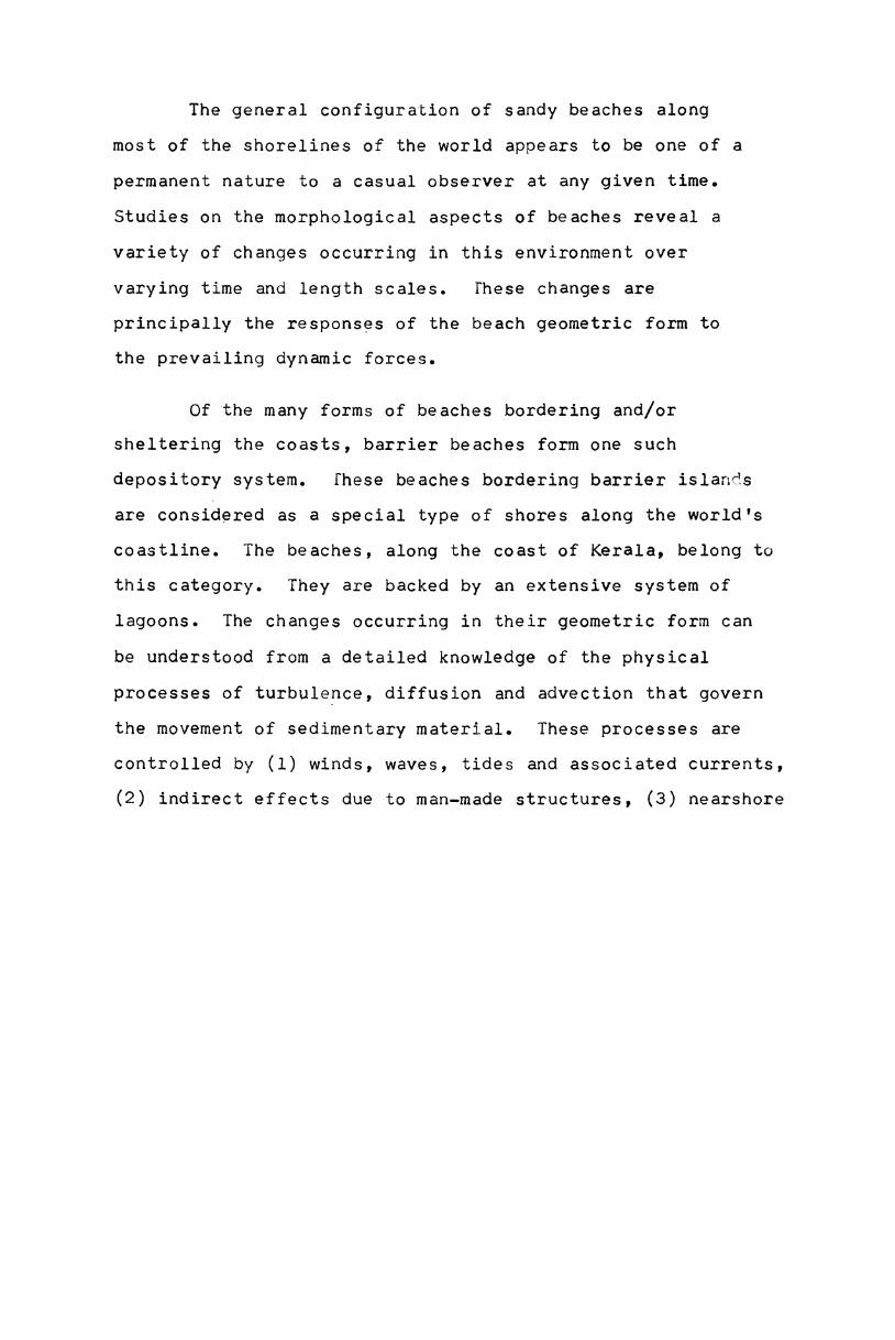
Physiography of the west coast of India.Distribution of the average rainfall over Keraladuring southwest and northeast monsoon seasons.
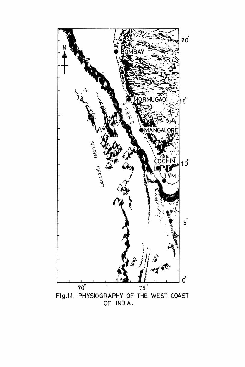
Monthly distribution of winds over Arabian sea.Shore protective structures along Vypeen andChellanam islands.
Map showing bathymetry and zones under study.
Schematic diagram showing beach terminology alonga barrier beach system and beach profiling.Spatial and temporal distribution of the empiricaleigen function at location Nl.Beach profiles at Narakkal zone.Beach profiles at Malipuram zone.
1
at Fort Cochin zone.Beach profilesBeach profiles at Anthakaranazhi Zone.Spatial and temporal distribution of theeigen function at Narakkal zone.Spatial and_temporal distribution of theeigen function at Malipuram zone.Spatial and temporal distribution of theeigen function at Fort Cochin zone.Spatial and temporal distribution of theeigen function at Anthakaranazhi zone.
empirical
empirical
empirical
empirical
Monthly changes of beach volumes at Narakkal zone.
Monthly changes of beach volumes at Malipuram zone
Monthly changes of beach volumes at Fort Cochin zone
Monthly changes of beach volumes at Anthakaranazhi zone
of mean grain size distributionAnthakaranazhi zone.
of standard deviation of grainsize along profiles at Narakkal zone.Monthly variation of standard deviation of grainsize along profiles at Malipuram zone.Monthly variation of standard deviation of grainsize along profiles at Fort Cochin zone.Monthly variation of standard deviation of grainsize along profiles at Anthakaranazhi zone.Monthly wave roses showing height and directionof wave approach off Cochin.Variation of refraction function along locationsA - T for waves approaching from 22OOTN.
Variation of refraction function along locationsA - T for waves approaching from 24OOTN.
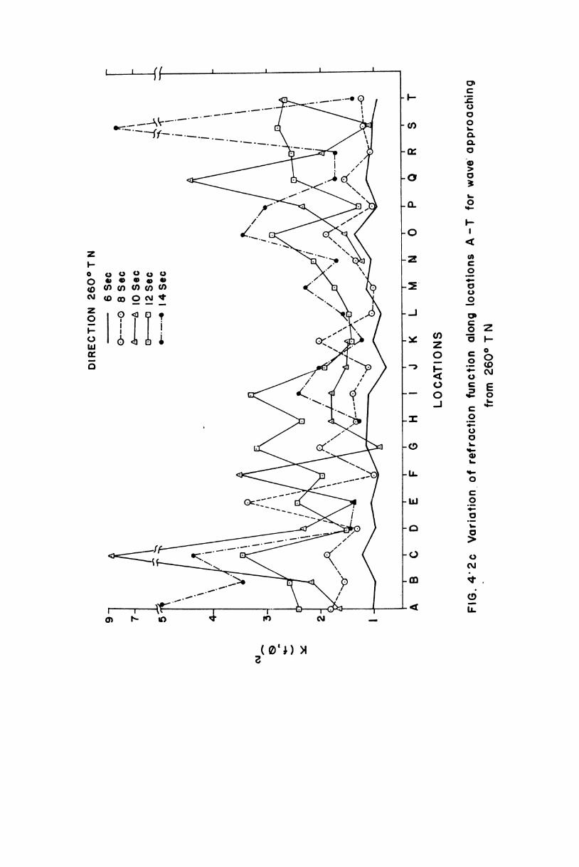
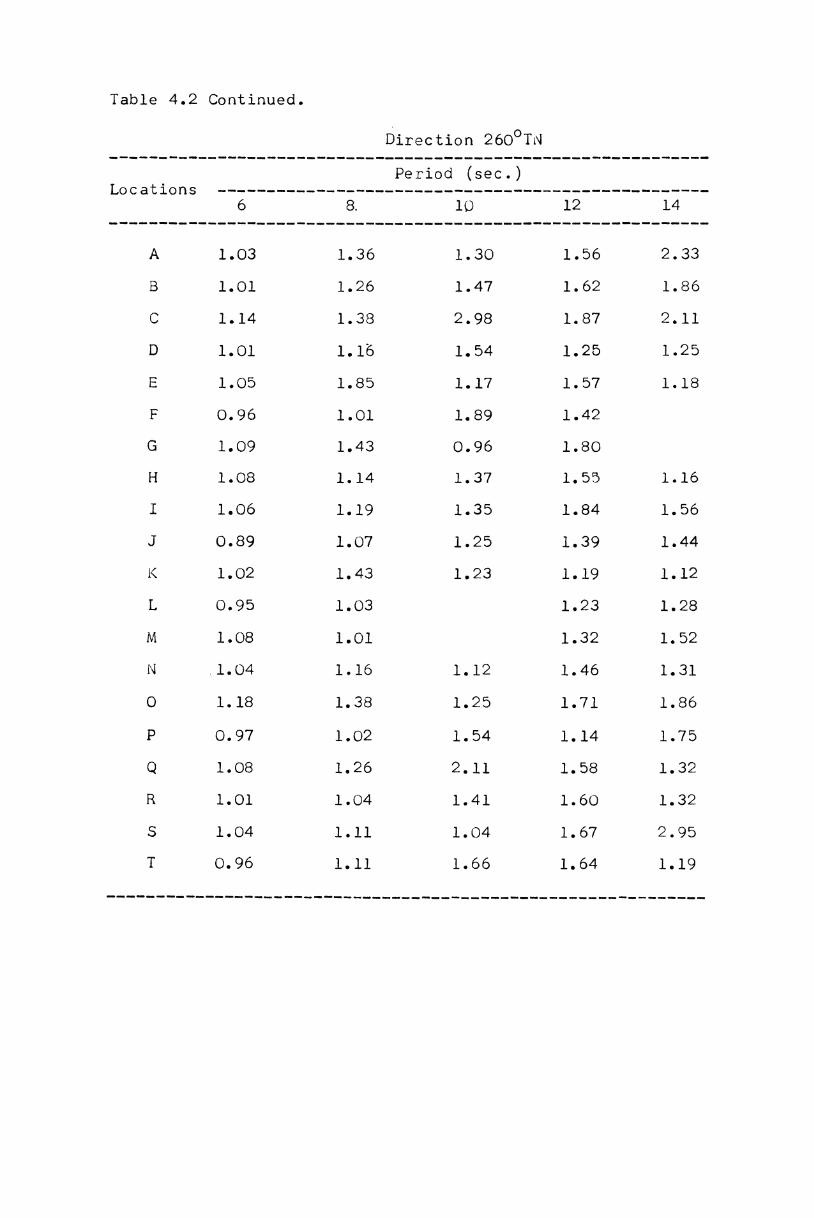
Variation of refraction function along locationsA - T for waves approaching from 26OoTN.
Variation of refraction function along locationsA - T for waves approaching from ZBOOTN.
Variation of refraction function along locationsA - T for waves approaching from BOOOTN.
Cellular circulation associated with waveconvergence and divergence for waves approachingfrom 22OOTN. .\ 'Cellular circulation associated with waveconvergence and divergence for waves approachingfrom 24OOTN.
5.10.
50]-do
5.le.
5.2a,
5I2b.
5.2c.
5.2d.
Cellular circulation associated with waveconvergence and divergence for wavesfrom 26OOTN.
approaching
9
Cellular circulation associated with waveconvergence and divergence for waves approachingfrom 28OOTN.
Cellular circulation associated with waveconvergence and divergence for wavesfrom 3OOOTN.
Distribution ofnear-shore zone
Distribution ofnear-shore zone
Distribution ofnear-shore zone
Distribution ofnear-shore zone
approaching
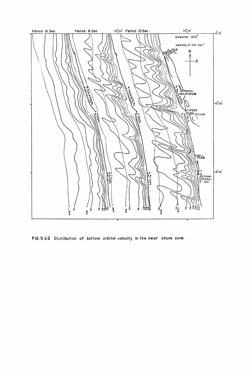
bottom orbital velocities in thefor waves approaching from 24OOTdbottom orbital velocities in thefor waves approaching from 26OOTN
bottom orbital velocities in thefor waves approaching from 28OOTNbottom orbital velocities in thefor waves approaching from 3OOOTN
2'1.2Q2O
4‘ 1.
4.2.
4.3.
4.4a
4.4b
4.4c
4.4d
5.1.6.1.6.2.
7.1.
LIST OF FABLES
Page No
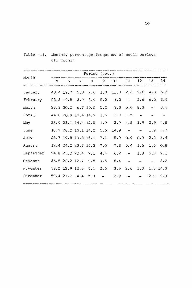
Details of beach profile locations. l8Percentage of mean square value of the dataas explained by the first three eigen values. 22Monthly percentage frequency of swell periodsoff Cochin. ‘ 5OValues of H/HO at 2 m isobath for waves ofdifferent periods and directions of approach. 53Direction function (O) for different periodsand directions of approach alongObserved breaker characteristics at Narakkal zone. 57Observed breaker characteristics at Malipuram zone. 58Observed breaker characteristics at Fort Cochin zone. 59Observed breaker characteristicsvatAnthakaranazhi zone. 6OObserved longshore current speedAlongshore component of wave energy. 77Computed littoral drift during rough and fairweather seasons. 79Thickness of bottom boundary-layer for differentwave periods and kinematic viscosities. ' 88
locations A-T. 56
and direction. 71
CERTIFICATE
This is to certify that this thesis boundherewith is an authentic record of the research carriedout by Shri S.Prasanna Kumar, M.Sc., under my supervisionand guidance in the School of Marine Sciences, in partialfulfilment of the requirement for the Ph.D. Degree of theUniversity of Cochin and that no part thereof has beenpresented before for any other degree in any University
<;/’i§::g;/$2 ~School of Marine SciencesUniversity of Cochin Dr.P.G.KurupCochin - 682 O16 . (Supervising Teacher)April, 1985. Professor in Physical Oceanographv
DECLARATION
I hereby declare that the thesis entitled,‘STUDIES ON SEDIMENT TRANSPORT IN THE SURF ZONE ALONG
CERTAIN BEACHES OF KERALA', is an authentic record of
research carried out by me under the supervision andguidance of Dr.P.G.Kurup, Professor, School of MarineSciences, University of Cochin, in partial fulfilmentof the requirement for the Ph.D. Degree of the Universityof Cochin and that no part of it has previously formed thebasis for the award of any degree, diploma or associateshipin any University.
M*“"°‘Physical Oceanography Division S "National Institute of OceanographyDona Paula, Goa. (S. rasanna Kumar)
ACKNOuLEDGEMENfS
I wish to record my deep sense of gratitudeto Dr.P.G.Kurup, Professor and Head, Physical Oceanographyand Meteorology Division, School of Marine Sciences,University of Cochin, for suggesting the research problemand for guidance and constant encouragement. I am alsograteful for his valuable advice and help in preparationof the manuscript and for suggesting improvements.
I am grateful to Dr.C.S.Murty, Scientist, NationalInstitute of Oceanography, Goa, for help in the preparationof the thesis. I am also thankful to Dr.Ramana Murty andShri A.A.Fernandez for their help in carrying out thecomputations. I wish to record my thanks to Dr.J.S. Sastry,Head, Physical Oceanography Division, National Institute ofOceanography, Goa and to the Director, School of MarineSciences, University of Cochin, for encouragement.
The help and co-operation rendered byDr.S.Sateesh Chandra Shenoi, Scientist, National Instituteof Oceanography, Goa, in the collection of field data andShri K.V.Chandran, University of Cochin, for secretarialassistance, are gratefully acknowledged.
-)(--X-*
CHAPTER l : INTRODUCTIUN
l.l. Geomorphology of west coast of India1.2. Shelf sediments1.3. Mud banks
1.4. Rainfall1.5. Winds
1.6. Waves
1.7. Tides1.8. Currents
1.9. Shore environmentl.lO.Previous studyl.ll.Present studyl.l2.Area of investigationl.l3.Scheme of thesis
Page
2
3
4
5
5
7
8
9
9
lO
12
l3
16
The general configuration of sandy beaches alongmost of the shorelines of the world appears to be one of apermanent nature to a casual observer at any given time.Studies on the morphological aspects of beaches reveal avariety of changes occurring in this environment overvarying time and length scales. These changes areprincipally the responses of the beach geometric form tothe prevailing dynamic forces.
Of the many forms of beaches bordering and/orsheltering the coasts, barrier beaches form one suchdepository system. These beaches bordering barrier islandsare considered as a special type of shores along the world'scoastline. The beaches, along the coast of Kerala, belong tothis category. They are backed by an extensive system oflagoons. The changes occurring in their geometric form canbe understood from a detailed knowledge of the physical
processes of turbulence, diffusion and advection that governthe movement of sedimentary material. These processes arecontrolled by (l) winds, waves, tides and associated currents,(2) indirect effects due to man-made structures, (3) nearshore
2
bathymetry, (4) weather disturbances giving rise tostorm surges and tidal waves, and (5) beach slope andnature of constituent sediments. The beach profile getsaltered depending on the balance between the above physicalagencies and the supply of material. Large scale irreversibletransformations, however, would lead to deformations in theshoreline configuration.
The environmental parameters that constitute thevarious physical process variables and contribute to thechanges in beach morphology along the coast of Kerala arebriefly summarised below.
1-l- GsQm@ren@lOqyOfwestcoastofIndia
West coast of India, the origin of which isattributed to faulting and uplifting during the late Pliocene(Krishnan, 1968), is bordered by the Western Ghats extendingto heights of about 1.8 km. These ghats, composed of rocksof Pre-Cambrian gneissie complex with thick laterite capping,fringe the coast from Cape Comorin in the south and extend asa range of hills, 24 to 28 km in width, over a distance of
nearly 720 km in a NNW-SSE direction (Fig.l.l) and providethe most important orographic feature of peninsular India.They are cut into a steep scarp on the west by faulting anddenudation. The distance between the scarp and seashore
{ _ { _{ \ _ A {§'>l3P.,?i"'~ Q:-"
3 ‘ V35/"'-;“..'_'g~\t\"_ °~ --' 0I " "5: A373"-1=12°| \ ;_*-.i"'A N ".:§k,_3-j=- O BAY ‘
3' { ‘4\ RMUGAQ) J;/_;‘_1_ fih ?\._ 7“-V3,_ -1‘ AA“
€\,5%
_ h' (§%i'5||r31' 10'_ ... “'4- ' TVM—
v gmdsu1¢
=5?/I11’
A >4
cfld
21- 3gJ- £- ‘$5 23- * ., 5/
%
\
si
nu
... E A\$’§ j _., 6§ 0.=~ 1 (I m | 41“ \ I I ,0O 070 75Fig.1.1. PHYSIOGRAPHY OF THE WEST COAST
OF INDIA.
3
varies from 8 to 4O km resulting in a narrow coastalstrip of alluvial deposits.
The coastal area of Kerala - the emergence ofwhich is legendarily ascribed to Lord Parasurama - ischaracterised by a strip of barrier land between Quilonand Cannanore which separates the Arabian sea from achain of long irregular lagoons and estuaries. Thisbarrier has a remarkably straight outer shoreline ofemergent nature and a highly irregular inner shoreline ofsubmergent nature representing the eastern margin of thelakes and lagoons. The entire coastal belt is backed bycoconut plantation and holds a dense population (550 per km2according to 1971 census, Kerala Government).
1.2. Shelf sediments
Along the west coast of India, the continental shelfhas a straight course and a gentle slope. It has a maximumwidth of l6O km off Bombay and narrows down to about 48 km
off Crangannore, north of Cochin (Fig.l.l).
The surface sediments of the shelf show well defined
zonation in the offshore direction. Broadly, seven zones nearshore sand, grey to olive brown mud, calcarious sand,foraminiferal sand, olive grey mud, grey mud and globigerinaooze - have been identified by Schott (1968). In general,
4
the distribution of clastic and non-clastic sediments(Nair and Pylee, l968; Kurian, 1967; Mattiat gt al., 1973)over this shelf from the shore could be visualized as:
Waterdepth(m) Nature of sediment
Q _3/6 18 1o8/144
l-3- Mud banks
3/618
108/144
270
Sands
Muds
Sands
Grey/black and white sand
Mud banks are regions of calm water appearing closeto the shore at certain locations along the Kerala coastduring southwest monsoon season. They act as natural littoralbarriers, influencing the sedimentation processes along thecoast of Kerala and directly affect the dynamics of theadjoining shore. The occurrence of these mud banks at fewlocations between Quilon and Cannanore is an annual
phenomenon (Bristow, l938). The available historical recordson the occurrence of these mud banks (dating back tol7th centuary) indicate their migratory nature (Moni, 1970).The sediments constituting these banks have been reportedto be essentially clays or silty clays and less commonlysand-silt clays or sandy silts (Dora gt_al., 1968). Theyare not charted on bathymetric maps.
5
1.4. Rainfall
During southwest monsoon season, Western Ghats
receive enormous rainfall forming the water—shed ofPeninsular India and play an important role in the climateof this region. Under the influence of the southwestmonsoon, which prevails for 3 to 4 months commencing from
May/June, the whole of the western region receives heavyrainfall. The distribution of average rainfall over thestate of Kerala during the southwest monsoon (principalrainy season) and the northeast monsoon (retreating phase
of the southwest monsoon) season (figure l.2) indicatesthat the coastal belt from Cochin to Calicut receives anannual rainfall of about 300 cm (Ananthakrishnan gt_gl., l979).As a result, the catchment area receives tr\ll3.4 x 109 m3 ofprecipitable water. Approximately 60% of this quantity isestimated to flow down as surface drainage (Prabhakar Rao, 1968]
directly or indirectly through the backwater systems to the sea.
Of the six major rivers - Periyar, Muvattupuzha, Pamba,Manimala, Achankoil and Meenachil - Periyar opens out directlyinto the Arabian sea while other rivers debouch into thebackwater system.
1.5. Winds
Monthly distribution of winds over the Arabian sea,obtained by streamlining of the data presented in KNMI
IOniI\gm Z<ZIW_~§<I_'Z<Z< 5:<;ZO2% ZOO®ZO_)_ 5fi__IEOZ_$M_>>'I5OW E0258 gig 5>O “E3 :6A _ _ 4om$5Am: Q5 Zoomz22¢ M045:\_ \ __O;DmE3_iv _ _VS 2 __\ ii I_ _ rQ_ kg “ on_ O _\__%°P __/______u°U AO _____ °m‘Ji____ ~__ l_\‘____8 ll ___T I.'_ __ _ __.O__.. . __- I ___\‘R O\ __’.KQ z_Iu0U_»\__‘ :__ I\_;° "_am__j(M“ }_ I f_'J YH __‘A_ _ |_ nU ___¢_____6E____M __ 0_\_ __I°md‘___" 13¢_ “'1 ___._":_.AJ.‘ \\‘ _‘__" J“_ fln_\{I*K A__ Q_‘Klr"___ O sU_J(°__ _’.___fl______U_d______\\‘. .‘~___\\,'.': I__/A tux\ON.LII’N ti)”~_____.’\-I‘!mu’1/ \\ I’~\ é_ on0*.2 it _y I‘ I nib‘ -m. \ I I _L._\. I‘ '\ I\\‘U\|_______o ______U3(uQ u¢oz*zz(U JfI I l_I __/__ h_~ \3“QNu‘_ 4& _E'\_‘.’:“-W@'_."\' \~.“ I_ r __‘___% - __'L_/‘JJ I UI_____‘_‘ q__ J '__).._‘\__ __(__ __ _‘F\_\____V Q HaJO 8% _W__J_____~\_ __' __. _|\ J‘ H.’ O n A“ ‘(P1_ (dV_°__§_ 2 t t %Z ___~\__” M“ OJ“ _A on t ,__1 _on B meg om B 207‘ Z \_fl£__ m_|~_°_O<_m_O w W M A _ O Z0: M 2°(Z2oz (U__ 0°”ANP\BPRP_llI]O2H6 Z 55 N___m u_ O6 _ _m _ A A\_ _ M mO 0m \@ X O i_’_N_Oz(>E.r <I O3_V ‘ {_U_ _ hr :°______6 \\\ _ O z°_____ _ m\ _______ O A 2 7_ r’ ’_ 8*O‘ 3 \ B NJ ( E__ |_ H G_“_n_ A_ Jwo_"_m 5‘toMWESZ?M ___N_TE
6
Atlas (1952) is presented in Fig.l.3. The characteristicfeature of the winds over this area is the reversal of the
wind system over an year known as the monsoons. Thisreversal occurs from south-westerly direction during May September, to north-westerly direction during December
\
March with transition periods in between.
During December and January, the winds are generallynorth-northeasterly in the northern parts and north-easterly
in the southern parts and blow with speeds of about 3 m sia.During February, they are mainly north-northwesterly and varyin speeds between 3 - 4 m s-1. Conditions are similar duringMarch but with a slight increase in magnitude and decrease in
stability than during February. Westerly winds with magnitudeof 3 - 5 m s—l prevail during April. During May, the windsare mostly from southwest and west, and have speeds from4 - 1o m 3'1. During June, July and August the winds blowfrom southwest with increased constancy and magnitude.West-northwesterly winds prevail in September. Octoberpresents highly variable winds, while north-easterly windsapproximately 5 m s 1 in magnitude prevail during November.
In the coastal areas, land and sea breezes areexperienced almost throughout the year except during thesouthwest monsoon season. The land breeze is well developed
and forms a part of the northeast monsoonal winds during
32: ___ZZv: 4% Z<_m<m< IU>O8;; "6 ZO_Sm_E_g 55202 2 _@_“_-\\‘_ Dl _J’ ‘II’ \~\\\‘ ‘R _ \ b ‘ ‘_ \\\\\ \' - " ‘ \ \- - ’ _‘ ‘ \ \ \' O \ -\ “‘ \ I-‘ \ \ \I ‘| ‘ \ I _ \ \ _‘ ‘ . ' ‘ \“ \\\ \\ " I ‘-'|‘\‘\ \\ \ _\ ‘ \ \‘-I ' \\\ ‘\ \\\\‘ ‘ \‘.‘ \\\‘ ‘ \\‘\ ' I .7_‘ . \\ \\ 4"‘ ‘\ \ \\ \\‘ ‘I V\\ _ \ ¢ \ _- ¢ ___ \‘ \ \ __‘ ‘ \ _“ \\‘ n \\ \_\ ___‘ .‘ I’ .‘ .‘\ \‘\‘ \\ n‘ ~ \‘. I ‘ \ \ \' 0 ‘ \ ‘ \_ ’ ‘I u \ __ ' \% \\ " _ ‘\‘ '. _ I ~__‘ 0 \\ \__ w_ ‘N ‘\\‘"""" \ ___ wag ' K: \‘\ b______W '_K _ Q \ \‘w" L.8 __ 8 .2 .8 ‘on .8\\‘,"h_ 0 é;"" ‘\ _ _ ‘ 'I N E __‘ __N _ \’_ ‘\ "'1 _ \' ‘\\ \\N'__ ‘ \\ _¢‘~ ‘ \_ ‘ _ ' ‘ N‘ ( ‘ ‘. \ \’ _' \ ‘ F‘ \ \ \’ ~‘ n _ \ “ \_ " \‘\ N \ (\‘ ~\ ( ‘I ‘\ \ ' . >_ . ’ \\__ ‘ __"\ \, I’, _' 0 ‘ R \\\ .0? ‘ i ', \ ' \\_~ -é N \ II ‘ I I \ “ ‘ ‘\ 1 \ "¢' _ \ \__m_ _ “ _ N _, _ ' N ’ _ \__' \ - ' _ ' ~ “ ' \““‘\ o J \ ~' \‘.M \ ONB‘ K‘ \\\| .6 _‘ d \ ‘ O é_ 3' ‘ ‘ ‘\\‘\‘ ‘ ' ‘s \ ~\\" ‘ ‘ \ h _ . I") \ \\ \\\ n ‘ ‘\ \““\\ ‘y ‘ I ‘.1 I " ' ‘N. “\\ \‘ I ‘ ‘\ ‘I ‘\ \\ ' ‘ I \ \ )‘ ‘ \ II’ \\ \ ‘.‘ \ T _ ’ I I .‘\‘\\ \\ \‘ '\ ' \ N \ \\\ _..\' \'-- I \ n‘ ’"-‘\)\_ _\‘I---‘U I‘\\L"_ ‘ \\n ‘Xx \ ‘\ \\‘\ _ \\\ A\ \‘\ __‘ \\ \“ E ‘ ¥ \\ \‘ _ _ ‘ 'N a. \\\ __'__ \\ ‘ _ .oi I \‘\ \ J _' ' H """ -- _h _\ ' ‘ \‘ _~_ \\ xx . @_’ I __ _ I \‘____ ¢ _ \\ F \\\\ N 1’ m “\\ \_N _ ' _ __ N __ __‘rt l‘ -\‘ \‘\ \\\\\ _ - __‘\\ ON \\_ ' _ I I ’‘N \ Emswao __ ___\ fimzgoz fl_/‘EL “M5050 .0“ I'M’ mwmzwtwm\ “ \ \ ‘¢ Q8 _ vv’ ’ ’ '8 I.8 ‘oh .8 ‘om ‘om .oN .8 ‘on ‘om ‘ON ‘ow .8 .0“ ‘ow .8l ' ‘_ \ /i bl ‘I," ' \ \\‘¢‘ ‘ \“ I.’ ' ~"' _\‘ ._ \\\ _' I I I’lI‘\l’\\‘% .8\ ‘ ‘ _‘J _\ " \U‘ ‘I,‘ ‘ ‘ \ I\__ ‘|-’\ ‘J \‘‘ ' _ V _‘I _\‘ \ \\\ ’ _ m _ _\ ‘_. _ _ \ "-\‘\\ ‘I I ‘I ‘ I§_ “ ..:‘\_\N é I \\: \_ _ ‘IO ' “' \‘‘ \‘\ w__ \ _' _‘ I - l-‘' ‘I ‘ ‘ __m ‘I0 .‘\ ‘ ‘\ _ _' \ ' s0 -\\‘ I!‘ '_' ‘ ‘ . |‘I --' .'. \ O.‘ \“'I A“ \‘)\ _\_ M’ __ .____‘__$\ E _8 _ :\\______\_ E‘_ 8 \_\n_ A _w~.2 .8 A ‘om .8 .2 _ 8 .8O _.‘oh 8 O8 _\ _ \\‘ M’ \ \1O _ I _\ \ ~\\ _v x: _\ \\\ s \\‘\ \\-"" -\.V 1 "1 \\ \\‘ “' 0‘ I \ _ \\\ ~‘ I \\ \\‘ ' \\\ ‘\‘ \\‘I‘\\\\__ _ \_ N 1 __m N r E _. ____\_‘_ k \ Q8 _ 7 __wN\ _
7
December and January. In general, the daily onshorewinds exceed offshore winds. The maximum onshore wind
speeds occur just after the mid-day.
l.6. Waves
Observations on waves published in the Indian DailyWeather Reports (IDWR) of India Meteorological Department
have been compiled b Srivastava et al. (1968) andY __.__Varkey gt_QI. (I982). The wave characteristics as seen fromthese studies indicate greater dependency on the prevailingwinds over the Arabian sea. Owing to the reversing windsystems, variable fetches occur from time to time with almostunlimited fetches on the southwest and west of this area andlimited fetches on the northern side. These fetches contribute
1
significantly to the generation of waves that affect thep
shoreline bordering this coast. Keeping in view theorientation of this coast (NNE-SSW), waves originating andpropagating towards the coast from 180° to 340° TN can beconsidered significant. The waves generated in the southIndian Ocean associated with cyclonic storms are also likelyto propagate towards this coast as long period swells.
In general, the seas present comparatively calmconditions for nearly eight months in a year and rough orconfused seas prevail during the rest of the year. One finds
8
a general increase in wave activity subsequent to increasein winds over this area. The waves during this phasepresent higher inconsistencies in their direction of approach
Data collected at Mangalore with the help of waverecorders during l968,'69 provide corroborative observations.The wave occurrence presents two peaks at 7 sec and l2 secduring December - February, sharp peaks at 7 sec and l3 secduring March to April, and almost a uniform curve with modearound lO sec during May through August. The significantheights of these waves are conspicuously high during June
through August. The significant period also shows anincrease during this period (Sundararamam gt al., 1974).
The data based on visual observation in the areabetween s°3o'u and ll°3O'N Lat. and between 73°3O'E Long
and the coast for the years 1974 - l98O have been compiledfrom IDWR and presented in the form of rose diagrams inChapter 4.
1.7. Tides
The tides in this area are of mixed semi-diurnalnature and fall within the micro—tidal range. They vary inrange from mean neap tides of 0.3 m to mean spring tides of
v
1.2 m. Noticeable variation in tidal range may occur by thecombination of surge and wave activity during rough weather
9
on the shelf. The current associated with these tidesattain speeds of about l.O - l.5 m s 1 in the vicinityof inlets. The fluctuations in water level associatedwith these tides affect the beach processes through (1)ground water and swash water interactions on the beach face,and (2) nearshore water circulation and morphology.
\1.8. Currents
The coastal currents have been reportednortherly during northeast monsoon months with0.5 m s 1. These currents, show a reversal indirection during southwest monsoon and presentvariability with mean speeds of l m s_l (HMSO,
1.9. Shore environment
to be
speeds oftheirgreater1975).
The shores of Kerala are in general sandy.At places they are backed by sand dunes and vary in theirwidth from 30 to lOO m. Based on available revenue records
for over lOO years, these beaches have been found toexperience erosion of varying magnitudes at few locations (eg.,Punthura, Thottapally, Purakad, Thumboli, Chellanam,Cheriakadavu, Manasserrey, Saudi, Fort Cochin, Malipuram,Azhikode, Crangannore, Chetwai, Cherai, Calicut and Bakal)resulting in recession of the shoreline and loss of valuableprpperty. The problem-has become acute during the last two
10
decades. The average rate of recession of shorelinehas been shown to be about 2 m per year at Purakad and5 m per year at Chellanam (Moni, 1980). As recession ofshoreline takes place at few locations, progression of theshore can be seen, particularly north of Cochin harbour(Vypeen), from available hydrographic charts.
In order to prevent erosion, shore protectionworks such as sea-walls have been constructed along certainparts of this coastline. More systematic efforts were madesince early fifties in this regard as could be seen from thefirst experimental sea-wall and groin assembly at Manasserynear Cochin (Fig.l.4). The design of the sea-wall has beenmodified from time to time and as of today nearly 70% of theshoreline of the coast has been padded up by artificialshore protection structures.
1.10. Previous studiesI
Earlier studies on beach and nearshore environmentalong the west coast of India can be divided into three maintypes. They are (a) studies to identify areas of erosion andaccretion through construction of wave refraction diagrams(Reddy, 1970; Reddy and Varadachari, 1972; Sastry and D'Souza,
1973; Gouveia gt 51., 1976; Antony, 1976 and Veerayya g§_g1.,1981), (b) studies on morphological changes at selected placesin relation to the available wave energies (Veerayya, 1972;
- PPURAM
01$; 6' LAND
KUZHUPPI LY
S
0"‘
E DAVAN AD
vYPEEN
O
-' NA 2%\- M\PEE
I
COCNN HARD R
MA ASERY
:@m@ W" itU
LAND
K NNA
S
jut
ANAM
bDAV
C
ODU
Scale 1"-= 2 mam
CHELL
' LANAM
F|'g.1.z. SHORE PROTECTION sw
Sea Wall with GrolnsIIII Sea Wall w
New Sea Wa
NAKULAMCOCH\ ERsauol _ D
ilh ul0 GrolnsCI] ll Proposed
RUCTURES ALONANAM ISLAND
0 VYPEEN ANDs. (AFTER AC
CHELL
HUTHAPANICKER, 1971)
ll
Veerayya and Varadachari, 1975; Murty, 1977 and
Murty gt 51., 1982) and (c) studies on the movement ofsediments using radioactive/fluorescent tracers (Manohar,1960' Gole and Tarapore 1966 and Nair et al 1972 etc.).
Along the coast of Kerala, studies on waverefraction in relation to beach erosion have been carriedout by Das gt Q1. (1966), Varma and Varadachari (1977),Shenoi and Prasanna Kumar (1982) and Prasanna Kumar gt Q1.(1983). Shoreline changes based on available historicalrecords have been investigated by Ravindran gt Q1. (1971).A review of erosion and shore protection works along theKerala coast has been provided by Achuthapanicker (1971)and Moni (1972). The morphological changes of the beachesat various locations along the Kerala coast have beenexamined for their stability (Murty and Varadachari, 1980),and for the efficacy of the existing shoreline structures byMurty gt Q1. (1980). Shenoi (1984) has carried out a studyon the littoral processes along the beaches around Cochin.
The physical aspects of mud banks including thesediments of the nearshore environs, particularly from regionswhere the mud banks are reported to be active, have beenstudied by Dora gt_a1. (1968), Nair and Murty (1968),
I
Varma and Kurup (1969), Moni (1971), Kurup (1972,l977),
Jacob and Qasim (1974), Gopinathan and Qasim (1974), Kurup
and Varadachari (1975) and Mac Pherson and Kurup (1981).
12
The above studies have indicated the susceptibilityof certain beaches of this coast to severe erosion duringsome years though they have been observed to recover duringsubsequent years. Further, erosion is not confined to anysingular locality. The zone of erosion and deposition havebeen found to shift from one location to another over theyears. The shore protection structure appear to have somestabilizing effect on the beaches at few localities whiledetrimental effects on beaches adjoining such structureshave been reported at many places (Moni, 1972; Murty, 1980).
l.ll. Qresent study
Sediment transport in the nearshore areas is animportant process in deciding the coastline stability. Thedesign and effective maintenance of navigable waterways,harbours and marine structures depend on the stability ofthe sediment substrate and the nature of sedimentation inthe nearshore zone. The nearshore zone is a complexenvironment and the exact relationships existing betweenwater motions and the resulting sediment transports are notwell understood. During the rough weather season, when thesediment movement is considerable, processes occurring inthe nearshore area are much less understood. Moreover,there is a general lack of field measurements, especiallyduring the time of severe storm conditions.
l3
The increasing pressures and the concern on thepreservation of the valuable coastal environment haveled to the development of shore protection programmes.Conservation not only demands knowledge of what needs to
be done, but also requires the basic processes to be fullyunderstood. Considering the fragile nature of barrierbeaches and intense occupancy of these areas by man, thesecoastal features have long been a subject of study bycoastal oceanographers, geomorphologists and engineers.
The present study is an attempt to understand thesediment movement in relation to beach dynamics, especiallyin the surf zone, along some part of Kerala coast and theresponse of the beaches to various forcing functions overdifferent seasons.
l.l2. Area of investigation
The area under study is a stretch of about 57 km ofshoreline from Azhikode to Anthakaranazhi (Fig.l.5).Azhikode, where river Periyar opens out into the Arabian sea,is located on the northern side. The Cochin harbour entrancechannel is located mid-way between Azhikode and Anthakaranazhi.
The navigation channel of Cochin harbour consists of 6 km longapproach channel, oriented along an eastwest direction and
two inner channels - 3 km long Ernakulam channel and 4 km longMattancheri channel - inside the backwater system. The
76' 00' 76.15’
S3B.LlP~l N
E:¥;'.?:
+0.--_ 1\ 1N§ARAxAL‘ G‘ 1 MALIPURAMIfll
-an \ IA F‘? A B I A N SE A
'"5*'A§3 " ' 1460*-'-.'.'.a -."-;.-_-,I?~_7,-?'.‘\‘- Q ..' _% A ‘-I--',f'|_l¢jq'|§iAv~4eA|<1
FlG.|-5 MAP SHOWING BATHYMETRY AND ZONES UNDER STUDY.
L‘ \ ‘ .- “F‘ .F§‘..§.N.fH'Al<ARANAZH\ ['5\ 1
%‘3'§~"~;Yi
1 T 7_,".~._:,'_ , ..
A,B-S,T- Locations for Refraction function estimations.N1-N3; ; ' — ' ' '
l4
approach channel was constructed in 1928 by cuttingthe offshore sand bar about 1.6 km west of the coast.
Silting is a severe problem in the outer channel which isbeing dredged every year to maintain the required depth.
At Anthakaranazhi on the south - a seasonal opening existswhich remains open throughout the southwest monsoon season.
The strip of the coast from Azhikode to Vypeen (26.5 km) andCochin to Anthakaranazhi (30 km) form two barrier islands,
known as Vypeen island and Chellanam island, lying on thenorthern and southern sides of the Cochin harbour entrancechannel. The width of these islands varies from l.6 - 2.4 km.There are large stretches of paddy fields along the easternshores of these islands backed by backwaters. The land islow lying with a number of cross canals serving as navigationaland drainage channels. The coastal belt is congested withhouses and hutments in close proximities and coconutplantations extending right upto the beach face.
The bottom topography on the northern side of theCochin harbour channel (Fig.l.5).presents gentle offshoreslopes and waves generally break well offshore. South of thechannel, bottom slopes are relatively steep and enable thewaves to break very close to the shore.
At Narakkal and Malipuram, during southwest monsoon
season the shore is usually protected by the presence of mudbank. Considerable stretches of the shore between Fort Cochin
l5
and Anthakaranazhi are subjected to seasonal erosion.
In order to understand the sediment movement
within the surf zone in relation to beach dynamics, fourzones - Narakkal and Malipuram along the Vypeen island and
Fort Cochin and Anthakaranazhi along Challanam island - wereselected. The beaches at Narakkal and Anthakaranazhi were
\~._.__,...,
protected by seawall-groin assemblies. In recent years,the groins have collapsed and are out of function. AtMalipuram and Fort Cochin, the beaches are backed byseawalls. At each of the four zones a number of locationshave been selected for detailed field observations. Theseare shown in Pig.l.5.
The parameters monitored are: (l) beach morphologyat low tide time, (2) sediment characteristics along theprofile section from backshore, berm, foreshore and breakerzone, (3) breaker height and period, orientation to theshoreline and direction of approach of breakers, and (4) speedof littoral current and its direction. The observations werecarried out by undertaking fortnightly/monthly field surveys
to 15 locations, spread over the four zones under study,during the period from October 1980 to January l982, as a partof the coastal zone management programme.
16
1-13 - S_C;h_Q;In_e__ Of. either _'th;e’s_i_§.
The observations on beach morphology and analysisof the data using Empirical Eigen Function (EEF) techniquesare presented in Chapter 2. "The spatial and seasonalvariations of grain size parameters of the beaches arediscussed in Chapter 3. Chapter 4 deals with wave climateas obtained from analysis of six years‘ visual observations
reported by ships of opportunity and published in the daily K|l[' vi (J .weather reports. Refraction of waves and the nearshore_werecharacteristics are also included in this Chapter. Chapter 5deals with the wave-induced currents as deduced from wave
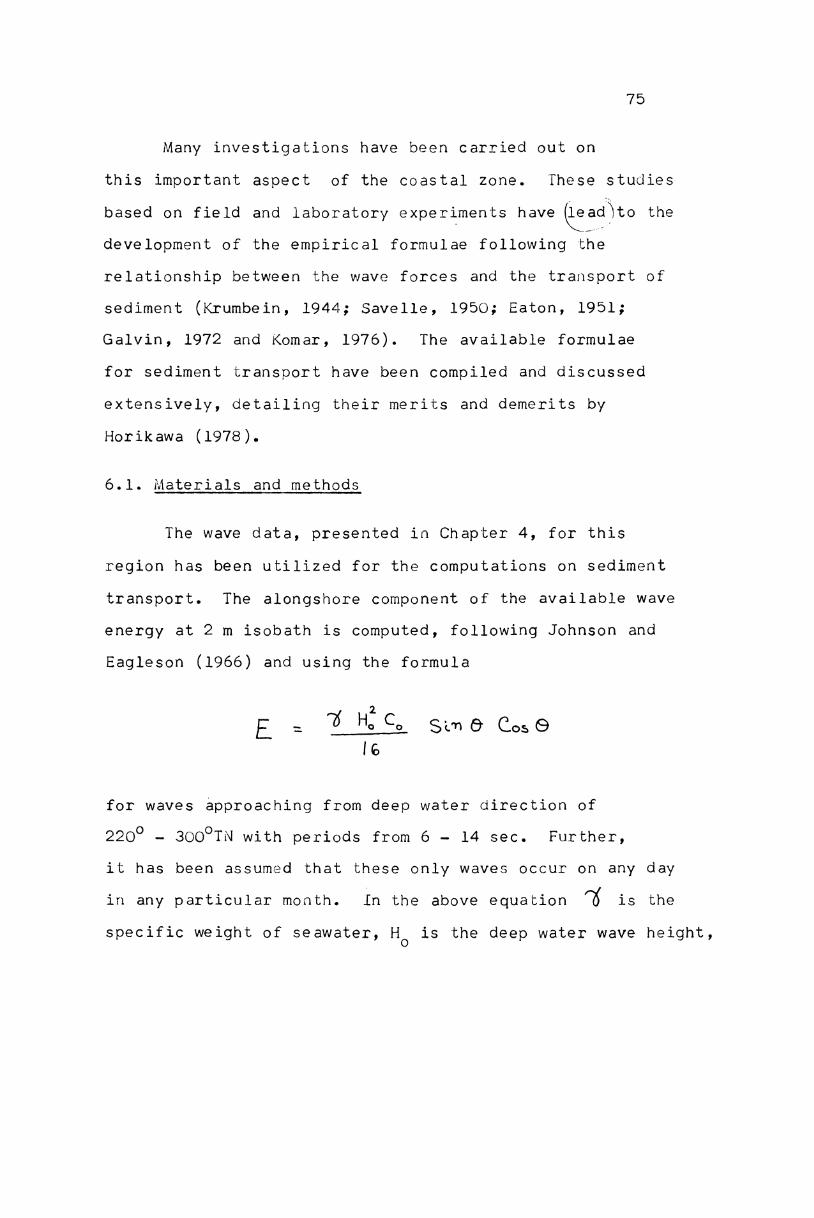
refraction studies and the bottom velocity distribution.The longshore component of wave energy has been computed
and the probable sediment transport has been assessed andpresented in Chapter 6. In the light of the environmentalprocess variables operating in this nearshore zone, thechanges in the geometric form of the beaches and the probablesediment transport within the stretch of the coastinvestigated have been synthesised in Chapter 7.
CHAPTER 2 : BEACH MORPHOLOGICAL CHANGES
Data collection and analysis2.l.l. Beach profiles2.1.2. Analysis of dataResults
Page
l9
19
19
2O
The interdependence of sediment movement, the
prevailing dynamic forces due to waves, winds and currents,and the resulting changes in geometric form of beaches wereindicated in the previous Chapter. In order to examine thesechanges, results of studies carried out on morphology of thebeaches at selected locations with differing environmentalset-up are presented in this chapter. Beaches, in all 57 kmin length, from Azhikode to Anthakaranazhi along the coastof Kerala have been chosen for this study. These beaches,composed of sediments in the fine sand-size limits and ofa low profile, are exposed to seasonally changing wind andwave climates. The stretch of the shore has been dividedinto four zones considering the environmental setting asindicated in Table 2.1. This shore is characterised by theopening of river Periyar at Azhikode on the north, the entrance
1
channel of harbour at Cochin and a seasonal opening atAnthakaranazhi on the south, all of which influence thesedimentation regime of this environment.
The method of measurement adopted for obtaining beachgeometric form at the fifteen locations (Fig.l.5) along the
8l.PC®m®HQ WMCHOHO Uw®Q®HHOU M UCQ PCQWQQMM Hflmgfiww @H0£; W4 pQ@UX®WCOHPMUOH Ham PM WPWHXQ q_Q v<HH®;m®w UQHHDQ _PC®w®HQ p< m_O m<COHQHUCOU UQOMEMU CH PDQ WPWHXQ m_O N<>HnE@Wmfl CHOH@|HHmgm®m _UC®w®CH% %O UQWOQEOU £Ufi®Q 30d.xC®Q USE >QU®pO®pOHQ >HH®HpHfiQ _HH®3®®w m_o>3 U®xUmQ QHM qm UCG mm_Nm b_OWCOHp®OOQ _UC®m EDHUQE %O _QUQWOQEOO £U®®n Sofis >H®>Hp®H®x m k mmW&Mm_UwQ @HO£wHm®Cwflp CO pwfixw wpwHWOQ®UU32 _m®>®g >3 U®uU®%%®CD m_Q Q2UCM ®HO£m¥UmQ wfip Ufifiswn @_O msHA0; WMWHXQ Hflmgfiwm _UC®m woo N2mCH% %O UQWOQEOO £Um®Q 30d_COw®@m COOWCOEgm UCHHDU ®>HPUM xfimn USEwig EOH% COHPUQPOMQ HMHPHMQm®>H®Uwm .U®mQflHHOU WCHOHU .wsp _wgQ@> QCQOQH CH _COHp®m m_O ml'HpW®>CH mflsp Op HOHHQ pfiwwmgg m O N7>HnE®WW® CHOH@|HHMgm®m _UCmwWCHM %O UQWOQEOU £Um®Q EOQQ Q “ _OD | Om >H£pCoE AV< @<|NM W<v H£NmCmHmMm£p:<I>HP£@HCpHO% AW%_®&_N&_H&V CHLOOU PhomO0 I O? I W IAwE_m§_NE_H§vm§ | mm >Hp£@HCpHOm | v |% EMHDQHHMEAmz_Nz_Hzv@m ' Om >fi£Pco2 A‘ @ ‘L HmM¥mHmZAEV &_m WCOHPMUOHCwwwfimfiwmwma £U_W@QEMMW HMMMMWMH MEHMMllllllllllllllllllllllll llllllllllllllllllllllllwmlmwmmgllllllllllllllllllmmmlmwmfiwgllllllllllllllllWCOHPQOOH @HH%OHQ £Ufl®n %O WHHGPQD _H_N QHQMH
l9
shore under study and the analysis carried out arepresented in the following sections.
2-l- Data ¢QLle¢tiqnandanaly$i8
2.l.l. §each_profiles
The beach profiles (geometric form) were measured‘ .following the technique of Emery (1961) for a period of16 months from October, 1980 to January, 1982 at fifteenlocations (Fig.l.5). These surveys were carried out atthe time of low tide at fortnightly intervals along theMalipuram and Fort Cochin zones and at monthly intervalsalong Narakkal and Anthakaranazhi zones keeping a constant
distance of 5 m between stations (Fig.2.l) along the profile.
2.1.2. Analysis ofédata.
From the data collected during these surveys, thebeach profiles were drawn using a HP lOOO computer. From
these plots, changes in the volume of sediments (m3 m'1 ofthe shoreline) were computed to examine the temporal variations
The profile data were further subjected toEmpirical Eigen Function (EEF) analysis to examine the timevariability of the beach responses. A brief description ofthe eigenfunction technique is given as Appendix (Page 106).
This technique'has been applied to the beach profiledata by Winant gt Q1. (1975), Aubrey (1978) andAranuvachapun and Johnson (1979) and helps in (a) separationof the temporal and spatial dependence of the data set ina way that it can be expressed as a linear combination ofcorresponding factors of time and space, (b) delineation
in space of the spatial location at which greater variabilityoccurs, (c) identification of seasonal or any other periodicvariations of specific nature which is otherwise lessobvious from conventional graphic analysis, and (d) identification of the processes responsible for the profile changesi.e., the presence of any specific events and their relativeimportance. In a way, this analysis would indicate clearlyseveral characteristic patterns of sediment movement on thebeach face e.g., the onshore/offshore and alongshore(Aubrey gt 31., 1976; Aubrey, 1979 and Clarke, 1984).Winant gt Q1. (1975) and Aubrey (1978) have shown that when
applied to beach profile data,_eigenfunctions have a physicalanalogue.
2.2. Results
Monthly beach profiles at each location along thefour zones (Table 2.1) have been presented in Fig.2.3 a-dwhile the results of EEF analysis are presented in
21
Fig.2.4 a-d. The monthly variations in the volume ofbeach material have been presented in Fig.2.5 a-d.
The eigenfunctions are ranked according to thepercentage of mean square value of the data (Table 2.2).The first eigenfunction explains the greatest portion ofthe mean square value. For example, at location N1, thefirst function accounts for 96.90% of the mean square valueof the data, while the second and third functions accountfor 2.94% and 0.07% respectively for the residual. Thisindicates that the contribution from the higher orderfunctions becomes negligible and hence they have not beenconsidered in this study.
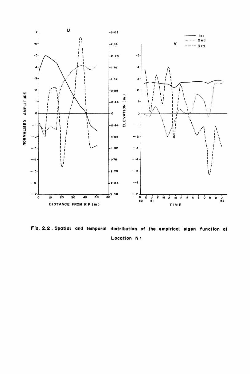
In order to elucidate some of the relevant features,distribution of the first three eigenfunctions at location Nlis presented in Fig.2.2. The first spatial eigenfunction (Ul)represents the mean beach function, analogues to the @f5Ufivarithmetic mean profile of the data. Its distributionindicates the presence of a berm and a moderately sloping
foreshore (Fig.2.2). The associated temporal function (Vl)shows the general trend and overall stability of the beachover the period of investigation. A constant value herereflects the near-stable nature of the beach underconsideration. In the present case, an overall increasing
Table 2.2. Percentage of mean square value of the dataexplained by the first three eigen values.
dr3Idan'2'\\ ..'_.\__‘J ‘.I! II\\‘\l \ .\I!\‘llll ‘D’ "_||’ll\‘\\_ ,____ fl_ IA5 M' ' O O I . I . . O .‘C ‘X\. \\\\\\ M\\ ..\ \ ‘ ..‘\ _'‘r ~."U ’ U ....‘liq‘! llI ' ‘ U UI‘ '‘Jill! ‘_\u‘\ ‘..\ .\\ .‘\ I..“‘_"_J!’ "IJ! V .-.( ._I .'‘\‘ .\ ‘I .\\‘ .‘ ..‘\\\‘\‘l\‘llIllll\\to2‘J8‘NisiA‘JidIniAV“IF_iJ%‘D_ #5 4O4_b__ _V_ W2 2 Ié _ l §_ \ \_n\ é_323_ _ F ‘ _ _2 4 O 4 2_ _“EV zo___<>u_m_N M M Nmy O 0 0 my_ _ _ _i6_i_4_64HO_?Na7_BO3.v‘!ll\ll‘\‘ .\I '. .II" lIll .I’!.||IIll\\\l‘\\\‘I.’-'llll":IIIIIII{lliv"!..‘U: ‘..'....‘. E“ I\\‘I‘...‘ _“\ . . . . ~ . . . . ...’.‘, __/I H.'|"II .'..::'¥".. \~\Yk‘ A \\:\ xx’I’\ll\ll}\\Or6IO5IO4Tw1”Fm1 _ fi T dfi7 6 5 4 3 __| 0 4 2 3 4 5 6_ _ _ _ _ _ _UODF____n_z< OUQJQZEOZl _ _ é A i _ _ Ho7EMHmRRMQRFECNATSDtOH.wtCUUfHOWOm_w___"Pm66htfOn_mtUbrthdMrOpmOtdnOMfl0PS22_m____F1NflMtOCOL
23
trend in the distribution of Vl indicates the possiblebuild up of the beach. The second spatial eigenfunction (U2),represents the berm function, and identifies clearly thespatial location where the beach profile experiences maximumvariability. In the present case, U2 shows maximum spatialvariability at the lower foreshore, near the mean low water(MLW 30-40 m) and to a lesser magnitude at the berm (Pig.2.2).The associated temporal function (V2) is characterised by astrong seasonal temporal dependence. The distribution of V2shows the overall depositional feature of the beach achievedthrough two conspicuous cycles of erosion and accretion.The third spatial eigenfunction (U3), which is the terracefunction, has a broad maximum near the mean low water. Thetemporal dependence of this function (V3) shows complicatednature, probably due to changes associated with thedifferential wave activity coupled with tide. Moreover, italso reflects that the low water itself is variable during the
'w
course of an year because of the seasonal changes in sea leveland erosion or accretion taking place at the beach under theinfluence of seasonally reversing wind and wave climates.
In the present study only two eigenfunctions and theirdistribution in space and time are considered since the profile
’
data did not cover the low tide terrace. The results of the
24
analysis are presented below to elucidate theintra-variations of the morphological changes alongthe four zones.
;é<>_11@r _-+_ ccllsarcslskal
The observed beach profiles (Fig.2.3a) at thethree locations in this zone show the presence of fullygrown berm at locations Nl and N2 at distances varying from5rl5 m from the reference point (R.P). At N3 such featureis not observed.
The mean beach function (Ul) at the three locations(Fig.2.4a) clearly brings out the presence of berm at Nl andN2. At all the three locations, the beach profiles showsteeply sloping foreshore which becomes more flat below themean low water (MLW). The temporal function associated withthe mean beach function (MBF) indicates an overallaccretional trend for all the profiles over the period ofstudy. However, the beaches at Nl and N2 present greatertemporal fluctuations compared to the beach at N3 (Fig.2.4a).
The distribution of the second spatial eigenfunction(berm function) shows that the variability maximum occurs closto MLW and with a lesser magnitude near the berm crest. AtN1 and N2, the maximum variability of the beach profile occursat the lower foreshore close to MLW, whereas at N3 this featur
‘ I I I * 1 I I I I I IO IO 20 30 40 50DISTANCE FROM R.P (m) \
FlG.2-30: Beach profiles 01 Norokkol zone
— _- K ~ ~ ~ _.-- ; m.w\ ‘“‘-1
\\\S\2:°\_‘\ D I0 — \' *--=-~l‘_‘.: ~5— ;m.w
MLW
-———- DEC ao
'------' JAN a|"—-—~" FEB1-----* MARA-———-A APR
A——-—-A MAY
¢>——-0 JUNE0-----o JULY0-in AUG:3----0 SEPC———C ocr/v------/v NOVD——-—-D DEC BI
l_TUDEAMPL SE1)NORMA
16-...
N2
.5 3.-/_' o
.4“.
.31
.2_.,
.|1
/\ u 1. .1. 1\' ‘..\. '-_ ...|.32 .3
-2'64
@2201 -116\_\ .
EVAT ON (m)
.\' '. -0-88\\. 1... 1\, .'-_. ._o.44 "
0\. ‘I...\ ‘ *00..
it‘ in
EL
\1,€.\. \N2N3 -o-447N1- 2~~ 1 1 ass -0 J: £2 ab ab 30 $5
'6-1
-6__
\-4__
-a
-zl
I unI E
U2
I'\1.1 '“'\,\~2if N3
0/ 9...
/5OCO
IIOOII
O
O
OOI0L _
_ . | -._.N I I
13%‘-. "'_!
'“2 N3
_.3_
_n4_
_u5a
_n6T
' 1on i
I
Fig. 2.4 a. Spatial and temporal distribution
1-1.0 1% £0 Q0 Jo do €bDISTANCE FROM R.P. (m)
Narakkal
VI
§~1 \ EN
ox. ft "30/00,... ...,I/' N3"2-n2
0,.
.|_,
.2__
.3_,_
.6__’o
“"1
| ...
2 ‘L 1 1 1 1 1 1 1 1 1" 1 1 1 1 rN D J F M A M J J A S O N D J80 8| 9|‘V2
1"
.1‘!
_1\.4-1 ‘I1 \.
3-.
io Moifjj. 1
\ ¢''\ {Z,
2
il 1 ti‘-_1 ' 1' ‘of 2 ‘ j I _ -.. \ . . I | \ |1 \ 1 i 1 1 ', -. W, 1‘, 1 1,
aJ
V '%ai.%?1 /Q, '
<:'
-5-. 0
1
I112 N,-7-*—1—'|-1 1 *1 1 I 1 1 1 F I 1 i*TN J A S 0 N D Jn 0 J F M A JI a230 8
THWE
of the empirical eiqon function atzone.
25
occurs below MLW. The second temporal function (V2)
indicates the short term cyclicity (of about two to two andhalf months period) of erosion and accretion to which the
beaches are subjected. Eventhough there is some phasedifference in the response of the beaches from November (1980)
to July (1981) the beaches behave in a similar way fromJuly to November (1981) and pass through a cycle of accretionand erosion.
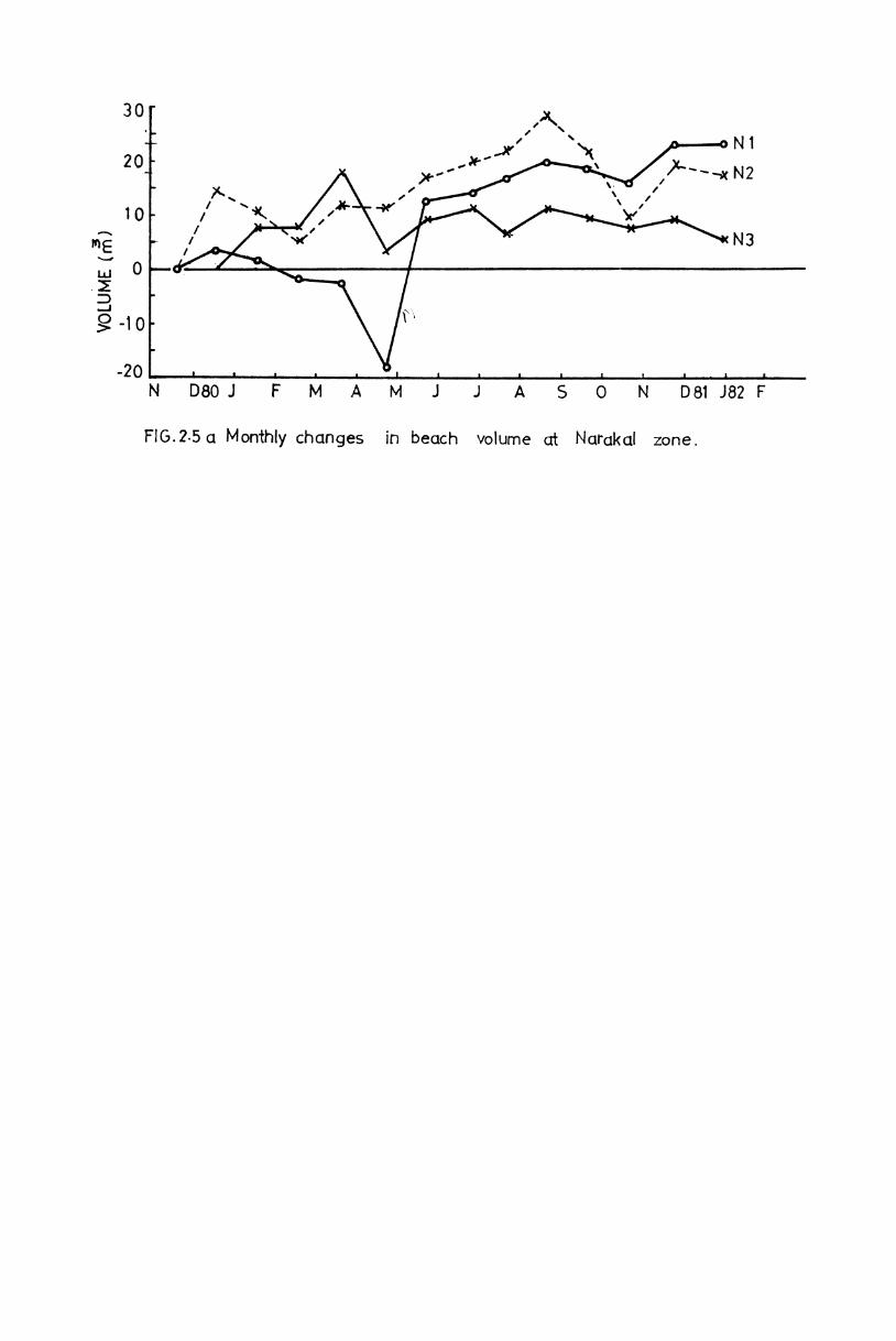
The volume changes computed from the monthly beach
profile data show accretion during November - December (1980)
at N1 followed by a period of erosion. This trend continues.till the end of April when the beach attains a level of minimumsediment storage of -17 m3 of material/m of the beach(Fig.2.5a). From April end to mid May the beach experiencesrapid accretion and recovers from the losses. Beyond May,
once again the beach passes through a state of erosion thatlasts till the end of October. During November-December,again the beach passes through accretion and erosion. Theoverall accretion amounts to 22.90 m3/m of material over the
study period.
The beach at N2 also behaves in more or less similar
way except during the period from February to end of Aprilwhen accretion prevails. The beach reaches the minimumstorage level of 5.5 m3/m of material during February (1981)
r-\
vowne (5
30
10
O
L.C)
-20
I
T‘
j\
$
/’\,,»*’ \ ' ‘N’*’w’ . \ }~~_\xN2/ \ //. .I
.I/?§\\ *1 \ I,/ X 3:’// N3, .
t_
iv
I 2 l1—e ~ -I ¢_,l ~l I P _l ,;J l , 4 1~—l _FIDBOJFMAMJJ ASOND81JFlG.2.5c1 Monihly changes in beach volume at Narqkql ZQne_
82F
26
but never goes below the initial level. The maximummaterial storage takes place during August (28 m3/m).The net accretion of beach at N2 amounts to 17 m3/m ofmaterial.
At N3, the beach builds up from mid December (1980)
till March, when it attains the maximum storage level ofl8 m3/m. After this the beach loses material at a rapid ratereaching the lowest storage level of 3 m3/m of the materialduring the end of April. Here again, it never goes below theinitial level. The subsequent changes are more or lesssimilar to those along Nl and N2. On the whole the beachgains about 5.3 m3/m of material.
Thus, both the EEP analysis and volume computationsindicate the fact that the beaches at Narakkal zone, ingeneral, gain material during the period of study throughalternate cycles of accretion and erosion. During the periodMay to December, the response of the beaches at all the threelocations are similar except for minor departures duringtimes of accretion. However, during December (l98O) toMay (l98l), the depositional or erosional trend indicategreater complexity at all the three locations.
27
Zens :1 Malipuram
In this zone, the beach profiles at each of thefour locations show the presence of a berm and a widerbackshore (Fig.2.3b). The location of the berm variesbetween 5-30 m from the reference point.
The distribution of mean beach function (Ul) alsoindicates the presence of berm (Fig.2.4b) and backshore atall these locations. The width of.the backshore, however,decreases progressively from Ml to M4. The beaches in generalexhibit moderately sloping foreshore which flattens out belowMLW. This is more conspicuous at Ml and M2. The temporalfunction (Vl) associated with MBF shows that the beaches atMl and M4 undergo greater variability compared to the others.Moreover, the beaches at Ml and M2 show accretional tendency
a’ \\_
while those atflMg)and M4 show erosional tendency.
The second spatial eigenfunction (U2) shows that at
Ml and M3, the maximum variability of profile occurs beyondMLW while at M2 and M4, it occurs at the lower foreshore.
A secondary maximum in the variability is clearly noticeableat the berm crest. The distribution of second temporaleigenfunction (V2) shows that the response of the beaches
in this zone exhibits considerable temporal variations,specially during January to June. But during June to December,
IIi ' _ . _:O I _ (;_/ 4. 1 O W7 7| ..I f ‘ t | ;-.
PM‘ '| ,1‘. ,_ .1I , :2 -. . 2 ..¢
—p
III
.1W $619 -1 F"-°- -"‘.
1 10%. uo¢'
0-i-,_
~.,__
\ I\ 0 01"‘ i A I 0-‘\ ' 5
1@—‘I"I0
- i .~_ I \ -_. '_ _‘i ' /I ‘\'. 1' 0 \ : I \I \ \ / \
-—n§_‘_-__
4III
-'3-‘W \\§__.’ ‘.1. 0~\ I\_ .. :_ ' \
I’..3\‘c
¢-'1'.
I ‘i ii
10‘..,,,-'-Q-L5
...Q.i
' '-mt’ \ \u4' 1
7777* 7 7 7* "'5*7i 771771 I I 1771 ifi |7i‘ '5 4* 1 71 ' i r J i i 1" 6o IO 20 so 40 oo o 70 no so 0 N J F M A M .1 J A s o N 0 Jso an a2DISTANCE FROM R.P( m ) .r|ME
Fiq.2.4 b,Spotloi and temporal distribution of the empirical oiqen function otMollpurom zone
28
near systematic accretional and erosional patternsare encountered.
The volume changes show that beach at Ml undergoes Qf\33L5gradual erosion till end of April when it reaches theminimum storage volume of -lO.5 m3 of material/m of thebeach. From end of April, the beach is subjected toalternate accretions and erosions with about one month
periodicity till middle of October, when it reachesthe maximum level of storage (28 m3/m of material). Then
onwards the beach loses material. The net volume change showsa decomposition of l4 m3/m of material over the period ofstudy.
At M2 also the beach initially experiences someerosion till January end while during February it builds upconsiderably. Once again, from March to May it erodes,reaching the level of minimum material storage of -7 m3/m.Then onwards it follows the trends exhibited by Ml. Thenet volume change amounts to a deposition of l5 m3/m of
material.
At M3 the beach is subjected to cyclic changes oferosion and accretion with roughly one month periodicity tillearly npril. Then onwards the beach loses material tillOctober when the beach attains the lowest volume of material
(-2O m3/m). From October to December, the beach experiences
_®CoN EU5Q___U2 g wg_O> 583 E WMUCULU 35:02 Dm_N_@__H_575QZO®<fifi_>_<z“_ 2\ / __\ ‘b// \ d," \\ I/ \ /_/Q // * Oq'°_"_qD’I ' Om‘III/I .I_ Id,I1 _ 7¥@®|M2 _|Nix‘\\I.I Illll <'1FAI ‘ dllM2 ,; I n\ _ //I _I W\ _ 3, \\ _ f /I” )\ . : I M. O__ \\\ wgX , \\ , \ 2:2 ‘x \ *1,’ XI \ X & /X LLI X‘‘ONJgm
29
one cycle of accretion and erosion. This beach reachesits initial volume level twice,initially during Februaryand later during April. Over the study period the beachloses material, amounting to 11.8 m3/m.
At M4, however, the beach is subjected to continuouserosion except during June to July and October to November.On the whole the beach loses 44.5 m3/m of material.
In general, the EEF analysis and volume computationshighlight the fact that, in the Malipuram zone, though thereis a wide variation in the response of beaches during Januaryto June, the beaches on the northern part (Ml and M2) andon the southern part (M3 and M4) behave more or less in asimilar pattern during July to December. Eventhough Ml and M2are subjected to alternate accretion and erosion, the netchange leads to a build up. At M3 and M4, the beaches do notshow much of an accretional tendency.
Zone - Fort Cochin
The beach profiles along this zone indicate thepresence of wide berm between 5 - 3O m from R.P, except at F4,where no permanent berm exists (Fig.2.3c).
The distribution of MBF (U1) shows that beaches ingeneral have moderately sloping foreshore except at F4,where they are comparatively steeper (Fig.2.4c). It also
~ ---- -'~ JAN em--—- FEB1+-----~' MAR.»--1; APRL-----0 MAYo——<>aum-:
Q-----<3 JULY
C+——c1 AUG0-----F3 SEPTc——-c ocrN------wnov0———0 oszc anj j r" \?"| “"1 71* *1 I 71 1" I 1 1 1I IO IO 20 30 40 50 60 TO
D"3TANCE r-"non R.P (m)
FlG.2'3c: Bench profiles ct Fort Cochin zone.
T Z’ (flBO
TUDEAMPLLZEDNORMA
--2-m
.5i
.4
.3__\
.2_.
.|._
\F4\\
F3
‘Q\_" 2 \\\ \--\\
U|
.\ .-..‘O ‘J-é\w"'.( .'¢ \°‘
lIOOll...\’ J I o O O5.‘.\ \_ "\ \F‘! \\ \_ _\\ . '\\ \.\ _\ 0\ \. xx \_\ \'\ ‘.0\ . '.
-avo
aoa
aaz
f'l'48
*0-T
6
~oO 1
v|-L
_ ‘\_ \w. _ L‘\_\\ \ \\F4 rs'\\“m,F2 h
“'2” W I i”“"i i * "* i I i ” * -48 '3“ ran: i t I *i *1 r r |~1 1*’ r-_r'—‘F'0 IO 20 so 40 J0 oo )0 ao 90 IOJ n 0 J F N A M J J A s o n 0 J rQ) 3| 82‘Uni
i
ii',--Q‘I \.4“
nucl
-.4...
-.5..
1/3-fl
I
U2
/' '\.\l1' _ ‘ ‘ ~ i.. ’ \\ ' -.\ 1.I II \- I J J4,-" ‘. "x,0’ I\ ‘I \s -',' ' f \/ i rs\2-w ’ .i I’ I . \
5' r’ to 1" rz r 1 i 'i'_f_'i'""T"'_i_I'“_T__iN 0 J F M A M J J A s o N 0 J FBO 6| B2TIME
Fiq.2.4 c. Spatial and temporal distribution of the empirical eiaen function atFort Cochin zone
3O
shows a step-like feature at Fl, F2 (at 30-40 m fromR.P) and F4 (at l5-20 m from m.P). In this zone, theslope of the beach below MLW does not show any change.
The temporal function (Vl) associated with MBF shows thatbeaches at Fl and F4 are subjected to greater variabilitycompared to those at F2 and F3. The overall trend of Vlindicates erosional tendency at Fl and F2 and depositionaltendency at F3 and F4.
The second eigenfunction (U2) indicates thatmaximum variability of beaches occurs at the lower foreshoreabove MLW, while a secondary maximum shows that at F3 the
upper foreshore and at Fl and F2 the step undergo variationsThe distribution of the second temporal function (V2) showsthat the beaches are subjected to accretion and erosion withvarying lags and leads.
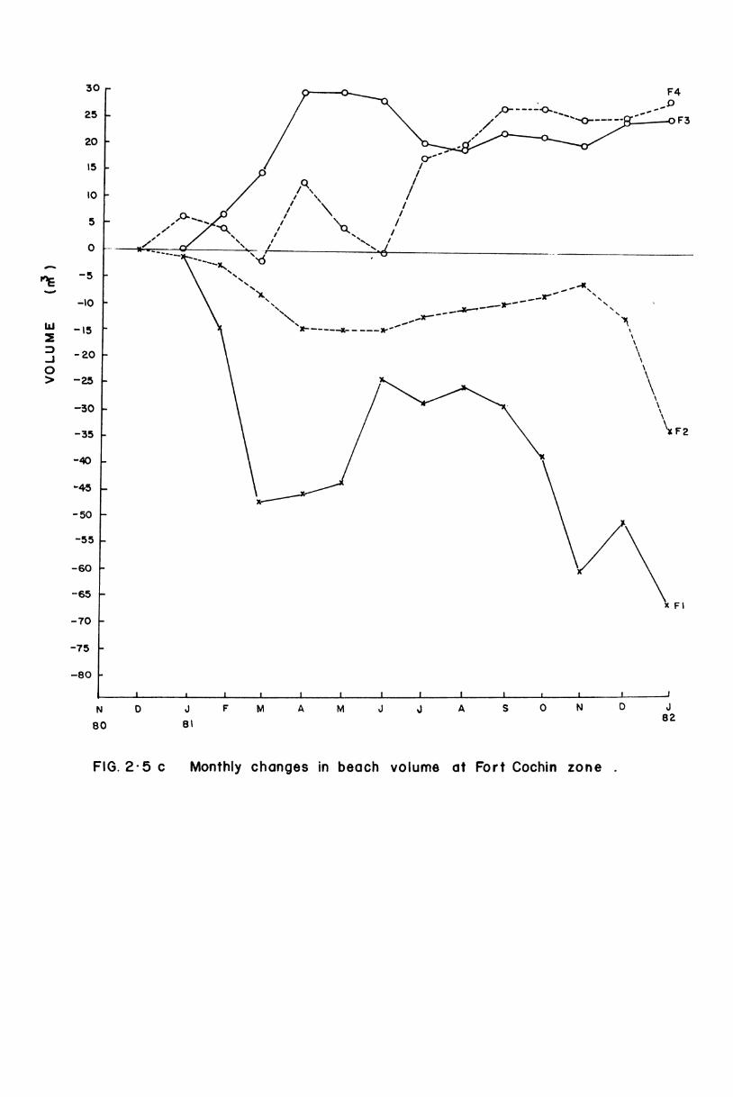
The volume changes show that at Fl, the beachloses material rapidly to the tune of 47 m3/m by the endof February (Fig.2.5c). Thereafter the beach experiencesaccretion leading to considerable deposition during May.But once again the beach loses material till December exceptduring November when it accretes. The volume change shows anet deficit of 65.6 m3/m of material over the period of stud
At F2 also, the beach loses material till March andthen onwards it slowly accretes till end of October. During
FIG. 2-5 c Monthly changes in beach volume at Fort Cochin zone .
L I J I I L I IN 0 .1 F M A M .1 J A s 0 N O J2so e\ 8
31
November-December, the beach once again erodes,
resulting in a net loss of 33.0 m3/m of material.
At F3, the beach experiences build up till March,resulting in maximum storage of 30 m3/m of material.From April onwards it loses material till July end andpasses through a cycle of accretion and erosion resultingin a net gain of 28.5 m3/m of material.
At F4, the beach is subjected to cycles of accretionand erosion with periods of about one and half to two monthstill May. From June to August, it again accretes and duringSeptember-November, it undergoes slight erosion resulting ina net gain of 30.0 m3/m.of the material.
Thus the EEF analysis and volume changes show thatthe beaches at Fort Cochin zone are subjected to accretionaland erosional cycles with differential lags and leads.
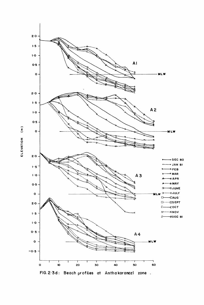
Z0 r1e,_.—. o-/insightel<.a,r-anaz,hii
The beaches in this zone exhibit the presence ofberm located between 5 - 20 m from R.P (Fig.2.3d).
The distribution of MBP (U1) also indicates thepresence of the berm (Fig.2.4d). [he beaches at A2 and A3have moderately sloping foreshore while at Al and A4 theforeshore is comparatively steeper. The temporal function (Vl)associated with ABF shows that beaches at Al and A3 are
E
ELEVAT ON
I
2'0-r
I-5 -I
1-0 -I
0.5 all
Q
2.0
I'5
‘.0 ...
0-5 -I
0-I-I
I
2'0 —-‘
I'O-*
0.5.. \ ~ K\\ ‘\ \_ _ _Q —~ —‘ c ‘\\’<g “*--N.._ - M Lw2'0-1
f the empirical eigen function atAnthakaranazhi zone
32
subjected to greater temporal variations. During thestudy period A2 showed maximum material losses.
The distribution of U2 shows that beaches in
this zone have maximum variability at the lower foreshoreabove MLW. At A2 and A4 the berm also shows some amount
of variability. The second temporal function (V2) indicatesthat the beaches in this zone respond in a similar wayshowing depositional tendency during January to April andrapid erosion during May to July. The beach once againshows recovery trend during the subsequent months.
The volume computations show that at Al, the beachis subjected to alternating accretion and erosion with aperiodicity of about one month till April and then suddenlyundergoes erosion during May to July (Fig.2.5d). The erosioncontinues till end of August at a reduced rate. The beachslowly recovers during September to November from the losses.Once again the beach is subjected to erosion during Decemberresulting in a net loss of 9.5 m3/m of beach material.
At A2, the beach accretes till March and showserosional tendency during April. During May to September,the beach loses material rapidly (about 80.0 m3/m). Thenonwards it slowly accretes till November. Again duringDecember the beach is eroded resulting in a net loss ofabout 30.0 m3/m of material.
II0
§J
VOLUME
"4
30*
25
20"
I5
Io
5
0 \
-‘O
\.\\:\\
\\s;
/ ‘’ \IIx-""""I
11
I1
II
II "£5flf
/F--_
§
J‘
A 3PI
III,’
I’,I\0. \1/ ‘\ /fa \\\ II \ \\ ‘\\
1I
I1\ \\ I\ \¥ a\ X
\
-5 _E
I____/__
40'
-5?#
J’jj;§
’¢|I,§’
III, x___ A2I “~1 ; ""\\ ’/ /
\\ ‘k {,5\ \5 1
I
\
\\
/,x'\\ /"’\ /I\ I,’{II I I I I L I I I IN D J F M A M J J80 3|
1
A
,’ A4,1\ \\ ,1’ \l\ \ / Al
*1 \I5 "" \ /I\ ,'20 —- \ \ '\ \\ \\-25 _ \ \ /\
30 *I35 " ll\ Ip I’\\ :,( ,1\ // \\ II\ 1 \B’ ‘\
'50
5
FIG. 2'5<I Month ly chonges in bea ch \nMu rne cn IX
I II 14S O N D J
rnhokuro nozhi ZONE
82
33
At A3, the beach undergoes alternate cycles ofaccretion and erosion with a periodicity of about twomonths till the end of April, after which it is subjectedto severe erosion till June. From July onwards, the beachaccretes and not only recovers from the losses but also showsa net gain of 2O.U m3/m of material.
The beach at A4 builds up, after an initial erosionduring December (l98O), till February. During March-July,once again the beach gets eroded. It accretes and recoversfrom the loss during November. The beach is then subjectedto erosion resulting in a net loss of about 3.5 m3/m ofmaterial.
In general, the EEF analysis as well as volumecomputations clearly show that the beaches of this zoneundergo maximum changes. The beaches show accretional
tendency during January to April, and then suddenlyexperience severe erosion during May to July. Then onwardsthe beaches show depositional tendency.
These observations can be summed up broadly asunder.
(l) The beach responses are, in general, variableparticularly at times of occurrence of accretion or erosion.
(2) At certain locations, the beaches experience erosionduring the southwest and northeast monsoon seasons.
34
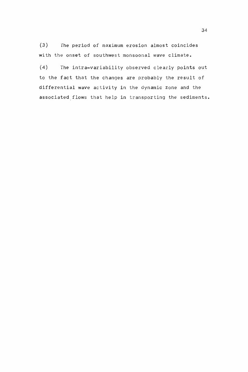
(3) The period of maximum erosion almost coincideswith the onset of southwest monsoonal wave climate.
(4) The intra-variability observed clearly points outto the fact that the changes are probably the result ofdifferential wave activity in the dynamic zone and the
ted flows that help in transporting the sedimentsassocia _
CHAPTER 3 : BEACH SEDIMEMTS
3.1. Materials and methods3.2. Results
The observed changes in beach geometric form along
the barrier beaches under study have been presented in thepreceding Chapter. This, however, provides only a part ofthe characteristics of the beach changes in this environment.In order to obtain a better understanding of these changes,one need to examine the sediments comprising the beach andthe changes they undergo as the geometric form of the beachchanges with\time. The nature of the beach material in theforeshore and inshore plays an important role in modifyingthe incoming waves through changes in resistance offered bythe sediments.
Beach sediments consist of masses of unconsolidated
sedimentary material on which the dynamic forces due to waves,tides, currents, etc. act. Under the influence of theseforces, the unconcolidated material gets sorted. The grainsize parameters are characteristic of the sediments and areimportant in the study of movement of nearshore material.The variation of these parameters along the beach profilereflects the energy levels to which the beaches are exposed.
The textural characteristics of the sediments and~their variations at various locations on the beaches between
36
Azhikode to Anthakaranazhi are presented in thisChapter.
3.1. Materials and methods
Beach sediment samples were collected by scoop
sampling at different stations along each of the 15 locationsat monthly intervals. The sediment samples were washed andoven-dried. A representative portion of each sample was thensubjected to size analysis by sieving, using a set ofstandard Endecott sieves arranged at l/2 ¢ intervals.Sieving was done for l5 minutes on a sieve-shaker. Thedifferent sieve fractions were then weighed and the weightpercentages calculated. When the samples contained materialof size less than 0.062 mm, the size analysis was carried outby a combination of sieve and pipette analysis following themethod of Krumbein and Pettijohn (1938). In all, 483 sampleswere analysed from the l5 profile lines. The grain sizedistributions were estimated by evaluating the descriptive
statistical parameters such as graphic mean (M2 ¢) andinclusive graphic standard deviation (<T¢), as proposed byFolk and Ward (1957), using TDC - 3l6 Computer.
3.2. Results
The distribution of mean grain size (Mz ¢) along theprofiles and their standard deviation (67¢) in all four zones
37
are presented in Fig.3.l a-d and Fig.3.2 a-drespectively.
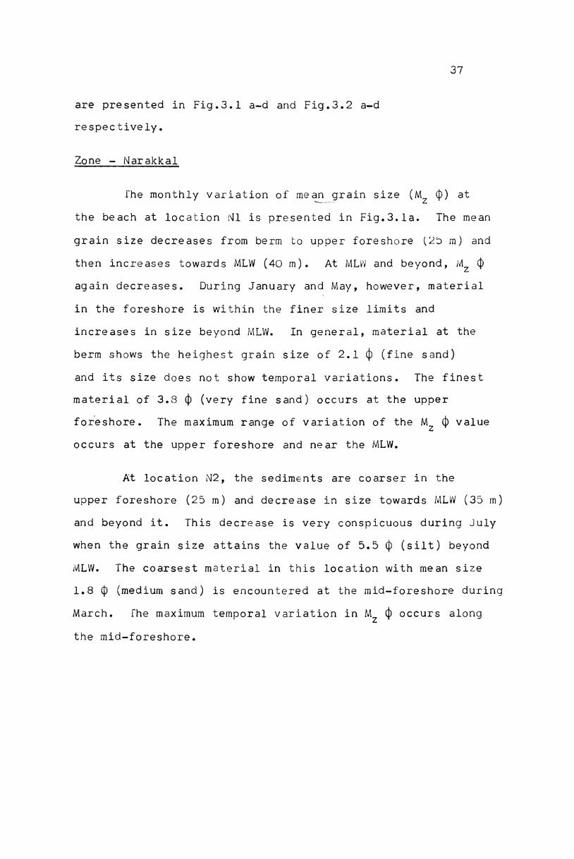
Zone - Narakkal
The monthly variation of mean grain size (M2 ¢) atthe beach at location N1 is presented in Fig.3.la. The meangrain size decreases from berm to upper foreshore (25 m) and
then increases towards MLW (40 m). At MLW and beyond, M2 $again decreases. During January and May, however, materialin the foreshore is within the finer size limits andincreases in size beyond MLW. In general, material at theberm shows the heighest grain size of 2.1 ¢ (fine sand)and its size does not show temporal variations. The finestmaterial of 3.8 ¢ (very fine sand) occurs at the upper
foreshore. The maximum range of variation of the M2 ¢ valueoccurs at the upper foreshore and near the MLW.
At location N2, the sediments are coarser in theupper foreshore (25 m) and decrease in size towards MLW (35 m)
and beyond it. This decrease is very conspicuous during Julywhen the grain size attains the value of 5.5 ¢ (silt) beyondMLW. The coarsest material in this location with mean size
1.8 ¢ (medium sand) is encountered at the mid-foreshore during
March. The maximum temporal variation in M2 ¢ occurs alongthe mid-foreshore.
0--0 D.EC 80_-.._ JAN 8|x—-—-x_,'FEBx--—-x MARPi-A_ APRor-—--A MAY0——0.. JUNEo----0' JULYG-——C'J_ AUG
[3-—--0. SEPTi-c , OCT
N——---N NOV0----0 DEC
O
F l ' I i fi I i i I I I gsO 5 IO l5 20 25 30 35 40 45 50 5 5 6ODISTANCE FROM THE REFERENCE POINT (In)
FIG. 3-Ia Monthly variation of mean grain size distribution alongprofiles at Narakkai zone .
38
At N3, the mean grain size of the sediment doesnot show appreciable variation from berm crest to mid-foreshore(25 m) except during July and November. Hence the sedimentsare within the fine sand-size limits. Beyond the mid-foreshore,the grain size shows slight temporal and spatial variations.
During July and November, the distribution of Mz ¢ shows anentirely different pattern. Between the berm crest and themid-foreshore, grain size increases to a maximum (1.8 ¢;medium sand) during July while it decreases to a minimum(3.8 ¢; very fine sand) during November. Beyond this,upto MLW, the mean grain size maintained the same values
during these months.
The distribution of standard deviation at Nl (Fig.3.2a)shows that in the upper foreshore the material varies fromvery well sorted class ((0.35) to moderately sorted class(0.5 - l.O). Beyond MLW, the material gets moderately sortedduring January and very well sorted during July. Except
during May (at Mrw) and July (20 m beyond MLW), the sedimentsbelong mostly to the moderately sorted class. At N2, alongthe upper foreshore, the sediment varies from very well sortedto poorly sorted class. In the lower foreshore region, sedimentshows moderate to poor sorting. Beyond MLW (35 m), standarddeviation again shows wide range of variation from very wellsorted to poorly sorted. At N3, material on the berm belongsto the well sorted class. The material becomes moderatelysorted towards MLW.
L "IE I t 1 I r | | 1 1 1 1 1Q 5 \O i5 20 2.5 30 35 4-0 45 S0 55 60 65DlSTANCE FROM THE REFERENCE POINT (In)
FIG. 3-2o Monthly variation of siondord deviation of groin sizealong profiles of Norokkol zone.
39
In general, the beach sediments at Narakkal zonebelong to medium (1 - 2 ¢) to very fine sand (3 - 4 ¢) andare of well to poorly sorted class.
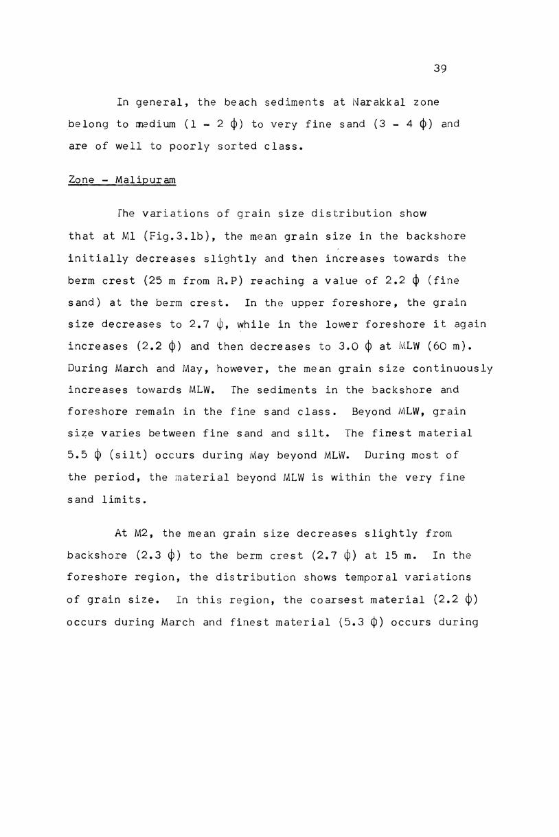
Zens--MaliPQram
The variations of grain size distribution showthat at Ml (Fig.3.lb), the mean grain size in the backshoreinitially decreases slightly and then increases towards theberm crest (25 m from R.P) reaching a value of 2.2 ¢ (finesand) at the berm crest. In the upper foreshore, the grainsize decreases to 2.7 ¢, while in the lower foreshore it againincreases (2.2 ¢) and then decreases to 3.0 ¢ at MLW (60 m).During March and May, however, the mean grain size continuouslyincreases towards MLW. The sediments in the backshore and
foreshore remain in the fine sand class. Beyond MLW, grainsize varies between fine sand and silt. The finest material5.5 ¢ (silt) occurs during May beyond MLW. During most ofthe period, the material beyond MLW is within the very finesand limits.
At M2, the mean grain size decreases slightly frombackshore (2.3 ¢) to the berm crest (2.7 ¢) at l5 m. In theforeshore region, the distribution shows temporal variationsof grain size. In this region, the coarsest material (2.2 ¢)occurs during March and finest material (5.3 ¢) occurs during
m,os
UJN(D
MEAN
2'0-*
1'5
3-0 -#
&5 -+A
4-0 -A
2'0-f
2'5
3'0
3'5-€
2-0-‘
N(IEl;
3-o_
3.5 -.
J»
O
4-5
200*
2'5-\
3-5
\/A
r* \ /' ,.\5'0 1 \\¢/f ,/"//
L________
M 4 /\_5:?“ E\\ \*~ J; $3 in 1 fi\\ I \\/\ \ / \\/ \ \
E Eli (Tim i?" I I IN ** I" 1 i i i i I i I0 IO l5 20 25 30 35 40 45 50 55 60 65 70 75 BO 85 90 95
3-lb Monthly vorlotion of moon groin size distribution olonq profiles atMolipurom zone .
4O
May, July and September. Beyond MLW (55 m), the grainsize varies between 2.5 - 4.2 ¢ (fine to very fine sand)with silt occurring during March.
The mean grain size at M3 shows an increase in theupper foreshore from 3.5 $ to 2.8 ¢ and then decreasestowards the lower foreshore from 2.5 ¢ to 4.0 ¢. DuringNovember, however, the grain size continues to increase inthe foreshore region attaining the maximum value (2.2 ¢)near MLW. Beyond MLW, the mean grain size decreases and
attains the lowest size of 4.5 ¢ during September.
At M4, the mean grain size increases in the upperforeshore reaching the value 2.3 ¢ and then decreasestowards MLW (40 m). But during September and November, the
grain size shows a decreasing trend in the foreshore. Thusthe sediments are composed of fine to very fine sand in theforeshore and fine sand to silt beyond MLW.
The variation of standard deviation, at Ml (Fig.3.2b),shows that in the foreshore, sorting varies between very wellto moderately sorted, though most of time it is in themoderately sorted class. Beyond MLW, the sorting variesfrom very well to poorly sorted class. At M2, the materialin the foreshore belongs to moderately sorted to poorly sortedclass and beyond MLW it is essentially in the poorly sortedclass. At M3, in the upper foreshore, material is moderately
I ','?flg——-¥i,P’4 _---—---"K0-e — / "' \“ ,/"">Y \/ Y4-_ ‘_<§\\ \ \\ \ ,v ‘K \\ \\ \ /O-4 .1 \ \\ \\ \\ //\\ \\ \\ \¢/4’ AO ' Z —- \\ //\ \V/L‘// I | i | 1 r i i 1* i i I I tj *1 *T* *1O IO I5 20 25 30 35 40 45 50 55 60 65 70 75 B0 85 9
oasnmce mom nereneucs r--mur ( an
FIG. 3-2b Monthly variation of standard deviation of groin size along profiles
41
sorted while in the lower foreshore it is between wellsorted to moderately sorted class. Beyond MLW, it variesfrom very well sorted to poorly sorted class. Sediments atM4 belong to moderately sorted class, except during Septemberwhen they are poorly sorted. Beyond MLW, they belong tomoderately sorted to poorly sorted class.
In general, sediment in the Malipuram zone belongs tothe fine sand to silt with sorting ranging from well sorted topoorly sorted class.
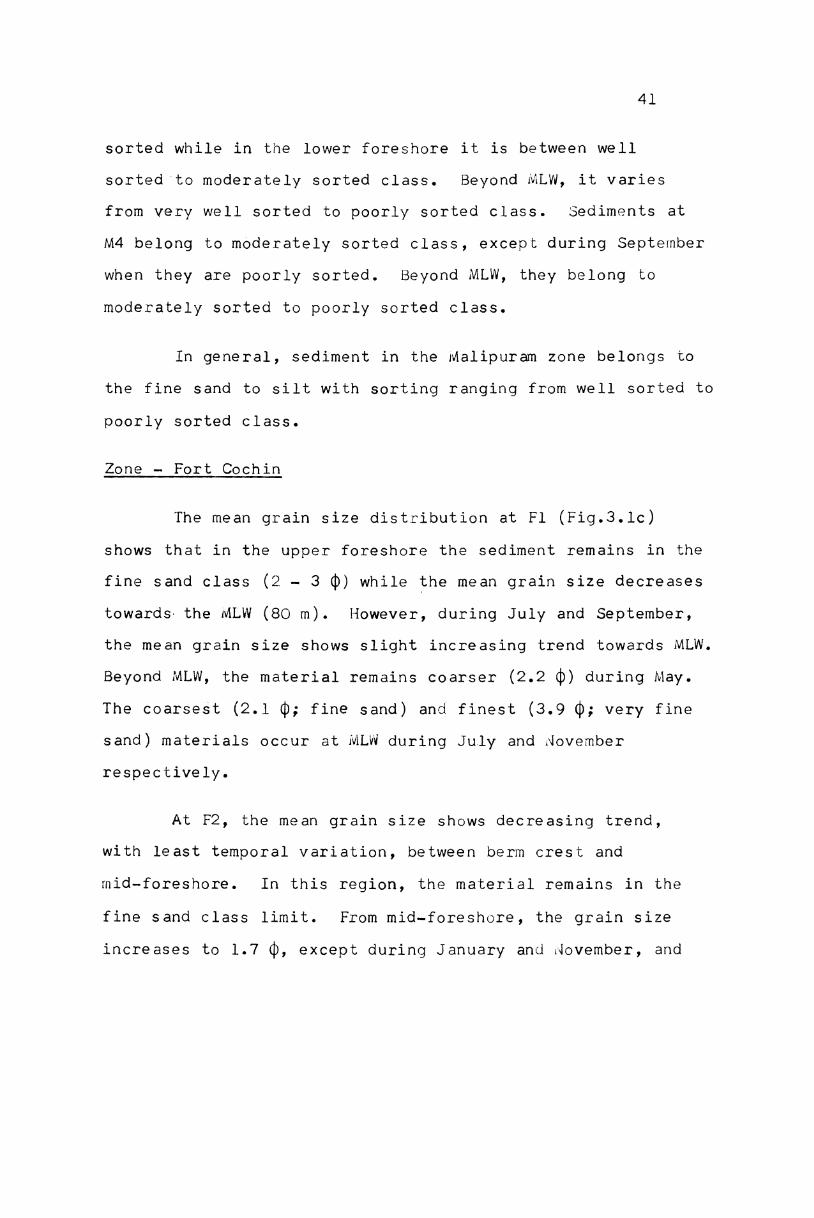
Zone - Fort Cochin
The mean grain size distribution at Fl (Fig.3.lc)shows that in the upper foreshore the sediment remains in the
fine sand class (2 - 3 $) while the mean grain size decreasestowards-the MLW (80 m). However, during July and September,the mean grain size shows slight increasing trend towards MLW.
Beyond MLW, the material remains coarser (2.2 ¢) during May.
The coarsest (2.1 ¢; fine sand) and finest (3.9 ¢; very finesand) materials occur at MLW during July and Novemberrespectively.
At F2, the mean grain size shows decreasing trend,with least temporal variation, between berm crest andmid-foreshore. In this region, the material remains in thefine sand class limit. From mid-foreshore, the grain sizeincreases to 1.7 ¢, except during January and November, and
it J{iii M1 U.‘ i §}i.__‘-._-ii: an-‘on-__cu-_<' _‘ § x )Z § §§_%
\ "‘§_;r/ Xi‘\N—~& --.. _.._k
\i-"'
---0
I I I I I I I I I I " I I I I I I I
or Fort Cochin zone .
0ls2o2:s30354o4ss0sseos57075906590 ooFIC-3.3-Ic Monthly vurloflon of mean groin size dlstribuiion along profiles
42
then decreases to MLW (70 m). The maximum temporal
variation of the grain size occurs at lower foreshore(60 m from R.P) where the coarsest material (1.8 ¢) occursduring March and finest material (3.5 ¢) dccurs duringJanuary.
The mean grain size at F3 shows a decrease frombackshore to berm where the sediments are in the medium to
very fine sand limits. From berm crest (60 m) to the lowerforeshore, the mean grain size increases, except duringJanuary and November. Prom lower foreshore to MLW (100 m),
the mean grain size once again decreases. The material inthe lower foreshore remains mostly in the medium to fine sandclass.
At F4, the mean grain size increases from R.P to the
step (at 25 m) and then decreases rapidly towards MLW (50 m).The coarsest material occurs at the step during March (1.55 ¢;medium~sand) and finest material occurs close to MLW duringNovember (4.7 ¢; silt). At the mid-foreshore, the temporalvariation of grain size from fine sand to silt occurs closeto MLW.
The variation of the standard deviation at Fl (Fig.3.2c)shows that the material remains in the moderately sorted classbetween backshore and mid-foreshore, whereas in the lowerforeshore upto MLW (80 m), the sorting varies between
(0'¢)VATONSTAN DARD DE
2'0-T
i'8-—i
0'8 1]
0.6 ..
0'4 -'
°'° '1
O-6 "T
0-4
0.2 _
|‘6T
|.4..¢
\-2 4
l-O
|.Q ... F3 /
f/
/1// "_/ 4*“/
'/
11-P
\\:7T_‘\§\\\
Q2////
Z-‘L----—-7-4:--O ‘\
\ CJ\> 5:":
@——-Q
M-——-x
——-x
‘“_'"fl
O'-"-OQ----O13*-C19---
"='="‘=""""""‘ / * I \\\x 0- -o\\\\ I \\\ §\N\ /\‘\-_-______ // \\
Q I5// 7 r* i 1 | | | | 1~ 1 ”“I | 1 *1 r I 120 25 30 35 40 45 50 55 60 65 70 75 BO 85 9 9"
F16. 3-2c Monthly variation of standard deviation of grain size alongprofiles at Fort Cochin zone.
43
moderately to poorly sorted class. In general, thematerial remains in the moderately sorted class. At F2,standard deviation values show temporal variations rightfrom the berm crest to MLW. The material remains in themoderately sorted to poorly sorted class. The material atF3 remains in the moderately sorted class all through thebeach, except during November when poorly sorted materialoccurs at the upper foreshore. At F4 the sediments arein the moderately sorted class, except during July, Septemberand November when poorly sorted material prevails at thelower foreshore.
In general, the sediment in the Fort Cochin zone iswithin the medium to fine sand class with moderate sorting.
Zo {leg W-_ Anth ak ar anazh i_,
rThe mean grain size distribution at Al (Fig.3.ld) showsa decreasing trend in the upper foreshore. The maximum temporalvariation of the grain size occurs near MLW (40 - 50 m). Thecoarsest material belonging to medium sand class (1.3 ¢)occurs beyond MLW, whereas the finest material (very fine sand)occurs above MLW during December.
At A2, mean grain size shows a decreasing trend fromberm crest to upper foreshore, varying from medium sand tofine sand, except during October when fine sand also occurs.From mid-foreshore to MLW, the material is in the fine sandclass limit.
f_
Q
§I
ll-I
NZ5
MEAN
3-0
2'O ..
2'5 ..
O
E
T
uh
-_
in
L
\
4
T‘
‘J.
‘IQi
l
1\
In
-I
A4
//0-------0\ //\\\\ I JV,A3
1‘ ’ /NI /"f _; ' ‘,. Z4" _ ifI’, ‘_____ /,4 \\_‘Q If“ i i i i i itic-K\;'| '
o—--oDEC 80-—--— JAN Blfiix FEB*-----IMAR1!‘-1 APR°--—-11 MAY°i0JUNE0--——0JULYC}?ElAUGQ---QSEPC?-<1 OCT"--——-N NOV0-—-—-0 DEC
\\\_A2
\g_‘.~ fi% }i \ ’. * "’ ¢Al
Q
\E : ‘GE_ in\\. ,8-— —— E“
P 3\\ /\ \4\ /\ //\ /\ /\ /\"U
0 5 no I5 20
FIG 3
t —l 1 f 1 1 | I * * 1 1 1 1 1 L125 30 35 40 45 50 55 60 6DISTANCE FROM THE REFERENCE POINT (mi
Id Monthly variation of me0n'groin size distributionalong profiles at Anthakoronozhi zone .
5 70
44
The mean grain size at A3, increases frombackshore to berm crest and decreases towards MLW (50 m).
The temporal variation of grain size is the least in thelower foreshore. Beyond MLW, the temporal variation ofgrain size becomes more, with the coarsest material (1.9 $;medium sand) occurring during April, and the finest material(3.4 ¢; very fine sand) during February.
At A4, the mean grain size shows greater temporalvariation along the entire beach. fhe coarsest materialoccurs at the upper foreshore (2.0 ¢; medium sand) duringAugust whereas finest material occurs at MLW (3.5 ¢; veryfine sand) during December. In general, the material remainsin the fine to very fine sand class.
The standard deviation of the grain size shows thatat Al (Pig.3.2d) the sediments are in the moderately sortedclass upto the lower foreshore. Beyond the MLW the sorting
become poor during April and December. At A2 and A3, thematerial remains in the moderately sorted class except duringDecember, when the sorting becomes poor. At A4, the materialalways remains in the moderately sorted class.
In general, in the Anthakaranazhi zone, the materialis of the fine sand class with moderate sorting.
I -fi A 1 1 r 1 1 1 | i I I #7 *5 \O \5 20 25 ' 30 35 40 45 50 55 60 65 70
3'2d Monthly variation of standard devlafion of grain sizealong profiles at Anthakaranazhi zone .
45
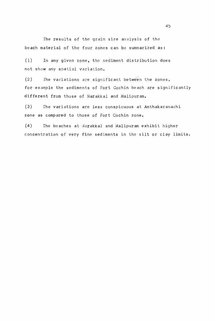
The results of the grain size analysis of thebeach material of the four zones can be summarized as:
(l) In any given zone, the sediment distribution doesnot show any spatial variation.
(2) fhe variations are significant between the zones,for example the sediments of Fort Cochin beach are significantlydifferent from those of Narakkal and Malipuram.
(3) The variations are less conspicuous at Anthakaranazhizone as compared to those of Fort Cochin zone.
(4) The beaches at Narakkal and Malipuram exhibit higherconcentration of very fine sediments in the silt or clay limits.
CHAPTER 4 : WAVE RQFRACTIOA
4.1. Materials and methods4.2. Results
4.2.1. Deep water wave climate4.2.2. Refraction function4.2.3. Nearshore wave amplification4.2.4. Direction function4.2.5. Breaker characteristics
All nearshore processes including beachmorphological changes are caused principally by the waveforcing in the surf zone. The changes in geometric formof beaches and their constituent sediments occurring duringthe period of study have been discussed in the foregoingChapters. An analysis of the prevailing nearshore waveclimate is presented in this Chapter.
Waves have been found to provide necessary energyfor the movement of water and attendant sediments within
the nearshore zone. They govern the evolution of beacheswhich act as buffer zones for the impinging wave energy.The shape and size of these deposits, in turn, give rise tochanges in the incoming wave energy through changes in thenature of wave breaking. When one considers the changes ofthis dynamic zone over a long time-scale, the dominatingeffect of waves in deciding the orientation of thisnear-elastic and energy absorbing zone becomes evident
In order to understand the shallow water wave climate,knowledge of the nature of propagation of waves into the shallowregion is essential. As the deep water waves approach the coast,
a changein theirshoalingof depthover the
47
in the wave height occurs because of changesvelocity of propagation. This is known as theeffect. Since the phase velocity is a functionin shallow water, when the wave front propagatesbottom of variable bathymetry, the wave front bends
and tries to get aligned to the bottom contours. This isknown as the refraction of water waves. Refraction causesconvergence and divergence of wave energy along the wave
crest. As the wave form finally approach the shore, thewave energy gets dissipated through shoaling, refraction,percolation and breaking. Much of this energy loss occursdue to the frictional effects. A knowledge of the wavefield in deep water is a pre-requisite to study the nearshorewave climate.
The wave condition in deep water can be defined bydata pertaining to wave field on monthly basis. This data,coupled with the effect of wave refraction over the shallowcontinental shelves, will provide the required input for thestudy of processes of sediment motion in the nearshore zone.
4.1. Materials and methods
The deep water wave climate was obtained by
statistically analysing the data available in lDWR's onthe visual observation reported by ships of opportunity in a30 square comprising the area under study for the period
48
1974 - 1980. The frequency percentage of occurrenceof wave height, period and direction of approach arepresented in the form of rose diagrams and table. Deepwater waves propagating shoreward from directions 2200 to
3OOOI§ with periods varying from 6 sec to l4 sec are likelyto influence the nearshore regions of the coast under study.
Wave refraction diagrams for the above periods anddirections of wave approach have been constructed for unitdeep water wave height following the method of Arthur gt_Ql.
(1952) making use of the latest hydrographic chart No,22O,published by Naval Hydrographic Office, Dehra Dun. Therefraction and direction functions have been calculated at
20 locations, fixed arbitrarily, along the stretch of thecoast from Azhikode to Anthakaranazhi (Fig.l.5). Thesefunctions provide an index for the relative amplificationor reduction of wave heights as the waves approach the CoastThe refraction functions have been calculated using theformula (Pierson gt al., 1955)
49
The ratio of shallow water(H) and deep water(HO)wave heights has been computed following Bretschneider (i966 b)
\/7’ F b -312‘__Pj_ _ to 1 °/b}%o _m:_ 1‘ \ fi- fiJm<j/Le _A A sin h 4-Fd l
Lw 4
In the above relations, bo and b are the distances ofseparation of wave rays, CO and C are wave crest speeds, LOand L are the wave lengths in deep and shallow watersrespectively and d is the shallow water depth. When thewaves break farther away due to caustics or instabilities,construction of refraction diagrams have been discontinuedat those depths. This.might give rise to some underestimation of the available wave energy at the final breakpoint.
The height, direction of approach and orientationof breakers with respect to the shoreline have also beenpresented on a monthly basis.
4.2. Results
4 - 2 - l - Qeee csweieli weave. Clsimate
A detailed examination of the fable 4.1 and the-wave
roses (Fig.4.l) indicates that the general direction of
firgm
HIIIIIII
E
%
%
EH
MARCH
’////é
FEBRUARYJANUARY
¢==\\\\
I|f|NI!§_
\\ )
5
.5
2-0
2-5
3-0
3-5
4-0
4 5
Q_ ' \éNX: \ii,‘ IfiflfivNNM¢' ‘WIJ5 IM
555:5
IHIH $2"//
5
‘OII
JUNE
3:’ 1.!”= '4
////\
APRL.
%\\///
////
///
2 @W
/////AI I I I I
.\Q
I @=IM *'_j_
@
7” " =#nn|m "/" \\ //,
@a
W‘
4%
éginfl fig”?0/,¢' § l I
‘\\\
Coch'napproach offton ofd'recshow ng he'gh1s andF0865WOV6Month y
-+
.<_-5
u.
O_No_No__90D_¢o_¢O _fiObD __E:qq<4@WU__g:§_________O3_ ______OO0 tO __OOO__n_a__ 2 8__O2__u Us _w___o§_ 05305 was 263 »_______o_Z __¢_w_“_D' WW WW \ ® _m__\\\_W\'\\‘ E" I \\\ _\\§ J __"”“H”_. ’ I‘\\\ _ ‘Nw“_____ __ _ /~ _ . . \\/4%N V‘ \§ _\ ‘ flan":M__mm"_ MwwmmmmmmmmQM‘ Em 1? _A____§ @\\\\\ha//v > ///_ Z ‘ . \‘ ‘ ‘ fig ’ \%M" I M \\\\_ _“__\__\ §mwmzmomo mwmzw>oz mumokoo. H” “W U __ W _____ ’ _$\__ I _ $ow “ ¢ W?Im_____WMm%m .m____WWWWmm.W ./Wx //1” I__> ;%%§‘ _\' _ _____ _ __ > ' CImwmzwkmmm Pwauaq *uDj
50
Table 4.1. Monthly percentage frequency of swell periodsoff Cochin
approach of deep water waves during January, Februaryand March is from NNW to NW (3000 - 350OTN). During April,
a gradual shift in deep water wave direction towards thesouthern quadrant takes place. During the period May toOctober, the waves approach from 2600 - 290OTN with increased
consistency. During November, a change in direction ofapproach of waves is indicated and the waves approach mostlyfrom 3000-350OTN. This feature continues till the end ofMarch.
During December to February, the wave heights aregenerally less than 2 m. By March/April, the waves attainheights as much as 3 to 4 m indicating a growing phase.Between May and September, the wave heights vary from 2 - 3 m
and show a further decrease to l m by 0ctober. DuringNovember, a slight increase is seen in the wave height.
4.2.2. Refraction function— t —__ ,_—e__ ,__
The refraction functions for the different»directions of approach calculated at all the twenty locations
(A to T) are presented in Fig.4.2 a-d. Waves approaching from220OTN (Fig.4.2a) show convergence and divergence of energy
in a similar manner for all periods except for l2 sec, whichgive rise to convergence at locations C, D and H anddivergence at E. For waves approaching the coast from 2400,all periods cause convergence and divergence of energy at
ZF “CNN E0:223033 263 be _T< 2o__8O_ 22° ___O__O_____; g__O_E2 *0 ___o__U__D> UN_¢_@_“___m”_afi_oz$_l_v____Io______________wZO____<UOJh_ U Q O D 4_ _ _ _ _TI D ‘mI I/ \ I Am’.I‘r ®I /_.\%_Vl:l®'ll 93 %Zgm ‘E Tlgm N_ TBgm o_ Igm m 0'16gm Q llZ___ 0 ONN ZO:_OUE_Q// \ /I \ ‘D’ \\ g ),’ fl g// \ /I \\ / \ X \ >_ \/OX . >0 \\ /I \\ X \ I \\ _ I G \\ 2 Ab__ \ 0 % /_ \\ Q Q I, \ ’ / \ _ _ ___ i./,7 4_ _ /\ __ Q //\:’__ \ / hm/ \ \ I \\ ‘ Z ’ \ / (‘Kbk It Q \ , 6 ¢ \\ l \n 4 __\ Q _ \ ’ 4 \ _ U__ __ X \ 3% \ MK __\ u / \ u / \ In Q/K’T_4L‘finLH)J(Z
2 F 00¢ N E0:g___OUOaa_u 263 BOwZO____<UOJ_F_'W”_Gn_OZ_)_|_V__J__ A_ A_ A_ _V ‘T4 MCO:OOO_oCO_O __o_8____; P_O_3U____2 O C“_ o_B_B> DNA“ _o_“_I __ O__ gm 3 ‘Ii. __ _ I____ IH gm ~_ Ulla uh Kgm o_ I K’ %L gm Q o_:|oawn ______l__Z___ °O¢N ZO____Ow@_Q‘_ I 0 “_ U O 0 m <L _ _ _ _ P _ _ _ A _ _ _ _ _ _L D q F IW / n ) \b/ ‘ 0 ‘\ VA I ° \ ° _\_»_ ‘Q Q M / Q \_\ B /_ /_ \\ ‘%B _ n 5 U _ 6 ’ O I‘ \ _L __ _\ _/ Q 6 _ Q \v\ 2 IQ __ __ Q N_ 4 Q x‘ _ \\ A O \Q l\_\ _/ \_ 4 _ \_ ,2 '_ \ _ X \ /IQ \\ M_ _ _ / _ ‘ _ _\ )K I ____ \_\ _/ \ Z __ \ NV n H’J B _ __ \ _/_ B 1 m Q/_ _ _ . _ _ \ /. (Z/ \ / \ ‘_ __/ _ ___ Q/\ / \ __ T __l \ ____ :_ \ __ ¢i % ) ‘no‘N
Z F 08“ E0:g___OOO_ag 22> __2 ‘T4 2O__8O_ 220 __O__2_e __O:8:2 *°____O:U_bO> ON_¢ _Q_____mZQ____<OOJ_IIIHm_IlM_________‘vf31______QZF_Pmman_o7__2|_v_______oh_mn_om_<_____?___L__________\\ I \ '°\ \ Q \ I_ _ d‘\‘_b/ % I I,4 / _L 0 ° 0 0nrv‘ 4 ll \ B II __ \ / w I, \\ ‘__ 0I n u \_ /o\ / 0 \ \ / Q \ I __ \__ / b/_ ‘L \ * __ _ I \ _ / _ I \ [I M_ IA /Q / \ I \ Q Q / \ _ /Q\ 0f Q \ \ Q‘ B d B ’ _ N/ \ _ ’_ \ ( / __ ’ 4O Q Q ___ __ B _\ Q ’ B0 _ a \ ” \‘ d Df u _ - \ __ __ f__ _ fl \_ '_&__ ,_ _ __ __ _ Z 4 _ __ 4_ \_ d Y I_ y \ I_ _ a \ Igm ¢ _ .'_|_|‘ FIlfigm ~_ Igm o_ Igm Q Qigogm w°O@N Zo____OmE_O4 \_ _&Tn_ _ _ |¢O_ IK /_/_Y“‘FlmX\’J0
7; OOQN E0:°___£OUOa% 263 3* __I-< _m___O___OUO_ o__O_U ___O:O__2 __O__O2__2 $0 CO:O:O> _uN_¢ ‘GIwZO____<OO___Fm E On_ OZEJ v_ ___ _ I @“__UD Om 4\__ gm 3 Tl W% gm ~_ I Igm o_ Igm m Glilogm 0 IIZ____ °OQN ZO_FOUK_O_ _ _ T _; _ \ _A _ _ _ _ _ _ _ _ L _ _ Ah0 F / 0 \ QK % I’ 4 :w in \\ 4 /// \\p// qr ___ : 7 __ i I 6 M \X ml b P‘ H 4 / 1 \\b\ \ $1\ /_ __\ Aw _ I, ___ a d\ 4n ‘{\ U __ d_ ‘I. __U __ u \_ ____ B A_ N\_ _ I __ __U _\.\ 1 / \_ G . ‘_\ /_ \U \ __ __ I. \_ I\\ O z ‘zL qM)J‘GZ
Z P OOOM EC:9___tOOag 0:; b2_ ___'( 20:82 206 ___O:_UC__; ___O:OU_;e *0 ___Q:U___O> @N_¢ _0_“_wZO____<UO______W"_Qn_OZ_2|_v____I@___UDOm<_ _ _ _ _ _ _ A‘ A_ l i _ 1 _\ _ L _ _; _IIT#H”1 ’ _7_/°/ \\\/ I \I MO/ ___ ‘Mr M4 ‘ 4n/2: _<>__ _\ 1 __: i . _\ /Ii Q _ \\ /1 \_5 /__ / \. 4 /Z4\®"‘O___-O O \Q‘ _> // iX B /m\’N /oi’/ 4 __ __ \%u\\ G I, I \I __ l ’l_%_B 1_ \ 1 \ _/a I _ V; I,_/ _\ 6/ \_,\ ___\ / _\_ U ‘8mN_ Qllm82: Igm Q ®::GZ ____ 0 QCD Zo_PUUI_Q25 3 I ‘i, _\/N / _\ _ /_ n\/K ‘Ill l ¢HHW_(Z
52
same locations (Fig.4.2b). Waves of all period producestrong divergence between locations J and M while strongdivergence is caused by waves of 10 and 14 sec at I and byl4 sec waves at G. Waves approaching the coast from 2600(Fig.4.2c) produce stronger convergence on the northern andsouthern locations while comparatively lower values areencountered along the locations in the middle zone. Therefraction functions have comparatively lower values at alllocations for all periods when the wave approach is from28OOTN (Fig.4.2d). When the wave approach is from 300oTN
(Fig.4.2e). Sfitrong convergences are produced by lO sec and5 I14 sec waves.
In general, the distribution of refraction functionshows wave energy concentration at the extremes of the areaof study for waves approaching from 2600, 2800 and 3OOOTN.
For waves from 2400, the wave height amplification takes placebetween location H and L. When waves approach from 2600,
which is a near normal direction of approach, the refractionfunctions present alternating highs and lows. The refractionfunctions show higher values for waves approaching the coast
ffrom southern quadrant than for those approaching from northern
O
quadrant with a general increase in the value with period.
4.2.3. Nearshore wave amplification
Table 4.2 gives the wave height at 2 m contour forunit deep water height for different periods and directions
Table 4.2. Values of YR = (H/HO) at 2 m isobath for waves
Locations
A
B
C
D
E
F
G
H
I
J
K
L
M
N
0
P
Q
R
S
T
of different periods and directions of approach
6.
1.15
1.31
0.95
1.19
1.o3
o.'39
1.43
1.13
1.35
1.12
1.1o
1.31
1.o3
1.o1
1.15
1.11
1.05
8.
1.41
1.61
1.26
1.33
1.69
1.01
1.54
1.14
1.43
0.98
0.98
0.96
1.55
1.09
1.38
1.03
1.34
0.93
1.34
0.95
Period (sec.)10
1.17
1.51
1.18
1.33
1.58
1.09
1.26
1.25
1.58
0.96
1.42
1.41
1.54
1.59
1.35
1.10
1.18
0.91
1.66
1.35
ODirection 220 TN
12
1.46
1.53
1.57
2.05
1.46
1.73
1.87
1.70
1.67
1.45
1.12
1.07
1.60
2.45
1.42
1.08
1.38
1.29
1.57
14
1.48
1.52
1.34
1.32
1.84
1.32
1.84
1.23
1.13
1.31
1.64
1.77
1.65
2.11
1.22
1.55
1.46
Table 4.2 Continued.
Locations
A
B
C
D
E
F
G
H
I
J
K
L
M
N
O
P
Q
R
S
T
6
1.21
1.15
1.15
1.21
1.22
1.04
1.02
1.08
1.43
1.01
1.10
1.08
1.06
1.22
0.98
1.14
1.16
1.08
0.99
1.05
8.
1.22
1.45
1.57
1.08
1.65
1.03
1.34
1.29
1.85
1.08
0.96
1.34
1.07
1.40
0.99
1.36
1.06
1.15
1.19
0.95
10
1.66
1.35
1.51
1.11
2.06
1.02
1.52
1.37
2.26
1.25
1.09
1.22
1.18
1.45
1.52
1.17
1.41
0.90
1.46
1.37
ODirection 240 TN
Period (sec.)12
1.14
1.71
1.88
1.38
1.48
1.35
1.98
2.05
1.88
1.25
1.25
1.28
1.25
2.05
1.73
1.33
1.84
1.31
1.o8
1.27
14
1.80
1.66
1.12
2.47
1.41
2.53
1.32
0.99
1.37
1.46
1.94
1.32
1.43
1.94
1.69
1.12
1.67
Table 4.2 Continued.
Locations
A
B
C
D
E
F
G
H
I
J
K
L
M
N
0
P
Q
R
S
T
6
1.03
1.01
1.14
1.01
1.05
0.96
1.09
1.08
1.06
0.89
1.02
0.95
1.08
1.04
1.18
0.97
1.08
1.01
1.04
0.96
8
1.36
1.26
1.38
1.16
1.85
1.01
1.43
1.14
1.19
1.07
1.43
1.03
1.01
1.16
1.38
1.02
1.26
1.04
1.11
1.11
Direction 26OOTN
Period (sec.)I5“
1.30
1.47
2.98
1.54
1.17
1.89
0.96
1.37
1.35
1.25
1.23
1.12
1.25
1.54
2.11
1.41
1.04
1.66
12
1.56
1.62
1.87
1.25
1.57
1.42
1.80
1.55
1.84
1.39
1.19
1.23
1.32
1.46
1.71
1.14
1.58
1.60
1.67
1.64
14
2.33
1.86
2.11
1.25
1.18
1.16
1.56
1.44
1.12
1.28
1.52
1.31
1.86
1.75
1.32
1.32
2.95
1.19
Table 4.2 Continued
Locations
A
8
C
D
E
F
G
H
I
J
K
L
M
N
0
P
Q
R
S
F
6
1.05
1.11
1.11
1.17
1.11
0.88
1.01
1.08
1.26
0.95
0.99
0.92
0.88
1.08
0.98
1.10
1.06
1.03
1.06
1.26
8 .
1.12
1.16
1.26
0.99
1.23
0.86
1.14
1.19
1.37
1.03
0.98
0.88
0.99
1.01
0.98
1.39
1.19
1.19
1.11
1.26
Direction 28OOTN
Period (sec.)10
1.15
1.3o
1.09
1.37
1.22
1.o2
1.30
1.17
1.37
1.24
1.15
o.s4
1.17
1.50
1.25
1.07
1.57
1.11
1.19
1.45
12
1.48
1.46
1.33
1.71
1.20
1.25
1.53
1.35
1.79
1.71
1.41
1.18
1.12
1.11
1.31
1.26
1.41
1.15
1.46
1.32
14
1.43
1.84
1.40
1.34
1.56
1.22
1.74
1.29
1.37
1.16
1.36
1.55
1.88
Table 4.2 Continued.
Locations
A
B
C
D
E
F
G
H
1
J
K
L
M
N
O
P
Q
R
S
T
6
0.98
1.10
0.91
1.05
1.03
0.79
0.88
1.06
1.16
0.86
0.84
0.75
0.89
1.01
1.07
1.07
0.94
0.97
1.10
0.99
8
1.07
1.23
1.69
1.12
1.14
0.91
1.19
1.08
0.88
0.91
0.89
1.12
0.99
1.37
1.07
1.55
0.89iii-Qj
Direction 3O00TN
Period (sec.)10
1.21
2.36
0.81
1.39
1.66
0.90
1.15
1.01
1.30
1.32
1.23
1.39
0.87
1.23
1.51
1.80
1.19
0.89
12
2.29
1.42
1.35
1.45
1.46
0.89
1.23
1.25
1.16
1.15
1.57
1.38
1.16
1.45
1.16
1.18
1.57
1.10
1.15
0.93
14
1.60
1.49
1.43
1.94
1.46
1.01
1.15
1.22
1.20
1.80
1.09
1.09
0.93
1.86
1.49
1.18
1.09
1.75
54
of approach. Waves of periods 6 and 8 sec approachingfrom 2800 and 300OTN, show reduction in wave height at 2 mcontour between locations F and M. For all other wave periodsand-directions of approach, amplification of deep water waveheight is indicated. In general, the amplifications in waveheight is more for waves approaching from 2200, 2400 and 2600
compared to waves approaching from 2800 and 3000 along many
parts of the shore under study. It is also seen that for somelocations, the wave heights have been amplified 2 to 3 timesthe deep water wave height. But these waves experiencinggreater mnplification might result in breaking before reaching2 m isobath through instabilities or caustics. Following the
limiting wave height Hb = 0.83d (Longuett-Higgins, 1972), themaximum height of the waves at 2 m isobath could be only 1.66 m.Fhus waves exceeding this limit would collapse prior toreaching the shore and subsequently expend the energy over awide nearshore zone through spilling or multiple breakers.For 6 and 8 sec period waves, the nearshore wave heights areless than the limiting wave height of 1.66 m at 2 m isobath.For heigher periods, the wave height exceeds this optimum valueat most of the locations.
4-2-4- Direetionfenstioe
The angle 0 made by the wave ray with the normal tothe 2 m isobath gives an idea about the direction of longshore
55
currents generated due to oblique approach of waves tothe shoreline. Angle measured towards north and south ofthe normal to the 2 m depth contour are indicated in Table 4.3with negative(-) and positive(+) signs respectively. Zeroindicates normal approach.
Comparatively larger angles are indicated for 6 secperiod waves approaching from both the northern and southernquadrants. Waves approaching from 2600, which is anearenormal approach, shows smaller angles. In general,there is a decrease in the direction function withincreasing periods.
4.2.5. Breaker characteristics
Breaker heights, periods and the angles of breakingobserved at all the locations along the four zones arepresented in Table 4.4 a-d. These observations at N1, N2 andN3 along the Narakkal zone indicate breaker heights ofO.2 to 0.3 m except during southwest monsoon period when
practically negligible or calm conditions prevail at N2 and N3.The predominanttbreaker periods are found to be 8 to l2 sec inthis zone. The breaker heights observed along Malipuram zonevaried from O.l to O.2 m. During southwest monsoon period,calm conditions prevail along this zone. Along the Fort Cochinzone, during southwest monsoon season more or less calmconditions prevailed at F2, F3 and F4. Along the Anthakaranazh
Table 4.3
Locations
A
B
C
D
E
F
G
H
I
J
K
L
M
N
O
P
Q
R
S
T
Direction function (9) for different periods anddirections of approach along locations A to T
zone, the breaker height.varied from 0.40 m duringnon-monsoon months to 2.5 m during southwest monsoon
season. The breaker angles showed much lesser valuesalong this zone compared to other zones.
CAAPYEH 5 : NEARSAUHE CIHCJLATIUN
5.l. Materials and methods5.2. Results
5.2.1. Cellular circulation5.2.2. Bottom orbital velocity’5.2.3. Observed longshore currents
Page
65
66
66
68
70
The observed sediment characteristics and their
temporal changes during the period of observation havebeen presented.in Chapter 3. The wave forcing whichcauses sediment movement has been analysed in the lightof nearshore wave climate and presented in Chapter 4.Before analysing the movement of these sediments in thesurf zone, the flow pattern induced by the incoming wavefield along this stretch of the coast is described in thisChapter.
Waves arriving from the offshore areas transportmomentum from offshore sources to the nearshore areas.
When waves attain a height comparable to water depth at any
point in shallow zone, they break forming a surf zone whereforces needed to resist the incoming flux of momentum are
established. Two types of forces could be distinguishedassociated with waves. They are the wave set-up and bottomshear. The former evolves as a changewin the time averageof water surface elevation while the latter is the drag feltby a steady current over the bottom. When the waves break
63
at an angle to the shoreline a steady alongshore currentmay be induced which would balance the bottom shear force.If this bottom shear force is sufficiently strong and if seabottom behaves similar to a movable bed, water will erode thesediment off the bottom and transport them to calmer areasfor subsequent deposition. This causes a change in thestructural configuration. In these cases, it is the sedimentthat receives the momentum. Once a particle is entrained bythe shear force, the vertical distance to which the sedimentwould get elevated depends upon the lift force originatingfrom the rotational behaviour of the grains of sediments,the size of the vortex and rate of dissipation of energy inthe turbulent portion of the boundary layer. Subsequentdispersal of the sediment is related to the impinging fluidforces.
, Within the surf zone, the swash and backwash transferthe sediments up and down the beach face, more so, in azig-zag manner and alongshore. These flows are verytranslatory in character and hence, make any extrapolationfor the entire stretch of the beach very difficult.
Realising the complexities in describing the flow fieldin the surf zone with a sufficient degree of accuracy, severalresearchers obtained different quantitative measures of field
I
64
of motion in relation to the breaker characteristics(Galvin, 1972). For example, several of the theoriesproposed for longshore currents are based on the concept ofradiation stress (Longuett-Higgins, l97Oa and l97Ob;Thornton, 1971). The observed cellular circulations havebeen found to depend on the longshore gradients in waveset-up as demonstrated by Bowen (1969b). These longshorevariations in wave height and wave set-up could be due towave refraction in shallow waters or the interaction of
incoming swell waves with edge waves. This wastheoretically and experimentally examined by Bowen andInman (1969) and the incoming swells have been found togenerate standing edge waves with periods equivalent tothose of the incoming swell waves. This interaction resultsin alternate high and low breakers giving rise to regularcirculation cells. The importance of topographically forcedcirculations have been demonstrated by Sonu (1972) andtested through numerical models by Noda (1974). The abovestudies, experimental or theoretical, have brought out theimportance of topography and radiation stresses in therealistic derivation of the complicated field of motionwithin the surf zone.
In this Chapter an attempt is made to describe theinferred wave induced nearshore circulation.
‘ _./
65
5 - l - Mauteur i also _;*a;r\__d_ umeihods
The wave height in the nearshore zone along thestretch under study from a depth of 25 m has been computedfrom wave refraction diagrams following Bretschneider (l966b)and using the formula
=H __.\ OH °L1._, \+4“‘*/‘1 f 5Ch\w14idL '2}\/1 b ‘/2Y" °/bK L0 c
From these wave heights, the orbital velocities associatedwith the waves close to the lower boundary-layer of thefluid column have been calculated using the relation(Lamb, 1945)
U _71H ‘iWflax “' —~"*" '*1' gfflh QfidL.
where Umax is the maximum horizontal component of theorbital velocity, H and L are the wave height and wavelength at water depth d, and T is the wave period. Thesevalues, which are significant in many ways, especially inthe initiation of the movement of sediment grains of a given
66
size, have been plotted and isolines drawn separatelyfor swell waves approaching the snore from 240, 260, 280and SOOOTN with periods varying from 6 to l2 sec.
The magnitude and direction of longshore currentswere measured during field observations by noting the timerequired for buoyant floats released into the surf zone tocover a specified distance along the coast (about 50 m).This is repeated thrice and the average value is considered asrepresentative of the magnitude of the longshore current.
5.2. Results
5.2.1. Cellular circulation
The wave induced flow field within the surf zone and
beyond in the nearshore regions is shown in Fig.5.l a-e.These flows derived from the energy available at 2 m isobath
are deduced from the convergence and divergence of waves asobtained from the refraction diagrams and reflect the natureof the field of motion due to the energy flux across theshore. This will help in understanding the up and downmovement of water with its attendant sediments from the regionof wave breaking to the beach face.
The distance of 2 m isobath from mean low water varies
widely in the area. This gives rise to considerable variations
° -0 ' °0> '0E? ‘-9 Qlo of: il
C
/ 3‘ ix‘Q \-/< \ \
4 S80 $330/"
h \
>9,
L‘
656>
ko
'\
‘ \ an
\
z<_|__. STPQRM N ° L ‘______,/v”/3J K K""§7~-»/"*-~"
G H ' <'>‘@“"”
O
ffl
\\
HC Z’ -/a '\~-1'/ A’-“'1 \\___..-/ ‘4Z(.:')l___,'(:.::'(~41 Z’ :’D\ ' \\ J \4r/-I/C3‘//7 u
4/" X /_z'a / _'€Z2' /}“)'/ KW/" /\l \__dz r’_\(.-I; R _"’/ -9
ECT ON 300° TNDR
d d verqenceOHwave convergence
.C.I:3
tedOSSOC OOHrcu atCCellular
lb
S2u.
67
in the width of surf zone assuming that all the incomingwaves break at this isobath. The flows deduced from the
available energy fluxes at this isobath indicate irregularand non-uniform motion. The flows are directed from the
regions of wave convergence to regions of wave divergence.In general, these flows present nearly closed cellular flows,clockwise or anti-clockwise, with large variations in svaceand time .
The flows associated with waves of 6 sec periodapproaching the coast from 22OOTN indicate larger circulationcells (Fig.5.la). As the wave period increases from 6 to lU secthe cells become larger in size and lesser in number. For l2and l4 sec waves, the cells occupy comparatively larger areasin both northern and southern stretches of the coast.
Q
For waves approaching the coast from 24OOTN (Fig.5.lb),
larger cells are obtained at the northern stretch of the coastwhen the wave periods are 6, l2 and l4 sec, while smaller cellsappear along the southern stretch (for almost all wave periods)except between K-N (for lO and l4 sec waves) and between Q+T(for l4 sec waves).
Waves from 2600 and 28OOTd (Fig.5.l c and d) generallygenerate larger cells for most of the periods. This featureis more conspicuous in the southern part for l0 and l2 secwaves (approaching from 2600) and in the northern part for
68
6 sec waves (approaching from 28OOTN). There is aclockwise circulation off Vypeen and anti-clockwisecirculation off Fort Cochin associated with 6, 8 and lO secwaves approaching the coast from 26OOTN, while the circulationreverses in its direction when the wave approach changes to28OOTN with periods l2 and 14 sec.
waves approaching from 3OOOfN with periods 6 and l2 sec
also produce large cells along the northern stretch. Waves oflO and l4 sec period, produce large cells at the southernstretch (Fig.5.le). For l4 sec waves, there is anti-clockwiseflows off Vypeen and clockwise flow off Fort Cochin.
In general, one notices the flow within this narrowzone to be consisting of cellular flow pattern, both clockwiseand anti-clockwise. These cells exhibit significant variationsin space and time.
5 - 2 - 2 - Be it Om? ;>,r_b.iJ_alrMs.l.Q2ij2>L
The flow pattern presented in Fig.5.2 a-d is based on thecomputed, instantaneous U values and indicates the maximumorbital velocities of the fluid particles inside the bottomboundary—layer of the fluid column from the shore to distanceswhere the water depths are 25 m. The distribution of the
Jmax values beyond 2 m isobath and upto 25 m provides information
_ 2 ON 20%_WE2 2: E r_Oo_2 _°:D__O EOEE.2mMmM 5_uw w _WM“60M6Z m O_ M*0 g_§__:2OO OO Nb _0EEN:gr;’I<Z<_____ /Z_ IUOU P,I_m¢] N8 _2'J9”AvZUWl>>_o@‘Q5_fT.QM 0' j aQ __ _’_ __'-_i‘ ‘‘_I__ _ __“Q __ Q ’_P /‘‘C \__Q‘H: \“I,z _‘0" n‘ _- "_ I4_~ “_’‘ L"3"‘"‘ '."". a/J J \\'II'___‘I’_If_ ,4 Mm“ 5 " at “I K/I I’E _ L ' Nu '//1 Q h__' _' ___‘ ' ‘ _u _7 ' I _\/ J/U ‘m‘ ‘ M w w 5 wM M € 1 __ N__ A __V‘ A I Md //“_ _ _;_/_/7 ' M“ W“ “___£_ _\_ Q ‘ W’ _____flU/_“ _ Q " WA’ N;___ "J __/_ H”I 3 ‘ _ M4 __l_’__ ‘ ” 0"_ _\ ’ ’ 2 ’ M! ___m_"_ / _ ____ I /J_ _’_ I ‘ I Fa t __/I, __0 EI Ifl,’‘_ \_\ T_\ _“’I VZA \__ r_8_0> “ “.0‘VN Z0;_n_ _m_0w~_.0:UUEO_ .‘ wk°__m;~_ "Bi3~_"_ I,I’ E //" J __ _W _ _ _ I *1 F _ ’ m:'_’__ ____I *2: __i f-‘ ‘J /_ X _ m _" u ‘ ~! @ __z:_____“__Jdi___ V ‘_ __ ‘ _M__ __“ \‘ ‘ 6: H 2'_‘va ‘@ I '_ __ , NH \ N2 \_ NZ ___ ”__ _ ___ Z _z \~»___.l ‘ \ \ .2 &_ ___ Z“id” "I ' P“ I’M IF‘ 4"’ ‘I’: ) ‘I’7 d, X / ‘ I‘ J_ _K ‘ ‘ I’ _ HT _ _ h_ ‘ ‘ K _ AM __ \_‘“‘ ’ __ € __N, V my _ ff\“‘\\\ J _ _U it “\\ M K xi ____T8” Eu ____ i? __M’/_/' *pl“_ égmo A,8% Q __v°___:_O ma ‘nus 4}E W _w I_ ’H___*__ _i “___ A A _'// _ ’_ “_v°___&f,__OQmQ H__°_=_n_ _
_ UCON 9_O____m 62 ____£____ :_OO_gOtonw w O*0 ___°_t_5Em_O Q NMLmwrw w 0mm/’ _‘ __ ___ gx ____”_6 M M6 O0 I2 83__ _2_n_° E_ mm ‘M w "M mm M__ I 4 ___‘_m6_''3 __IN<Z 2 __<I<¥<IF29“hm. W“ ___.8 M/_z€Z(JJ:0 "__‘__'I My"_5I__::T8“ E0 E“ :_8_Q>__oQN zo__6H__m_o_n_ ‘E{N I Li’‘GI_~§ __ _~Q_VWM 2 n‘l _'/My_ fi~{>‘__ __‘ _V ' _\_ “_~_‘ _) __"' 1JV?Q‘I "N! 3'nz ‘ \ _a_ _:i"_‘ ~_zz _\A“_AI id’I’‘I’J‘ ‘ II_z __%_ ,'_ \ fll_ _'/ ' HL ‘ /I’ / ’_' Z _d’ ‘ "'I’, _ ' I_ ,'1 X_ ;°wNgm N_ H__°___g_gm 9 "_v°___:_I __ _ ____ ;_”___I ____' ’ __'4 ’H__ :_ __‘ 2 3’2 _“ ‘_< k‘? ‘I3 __N1‘’_ C_ __'§"Igm w n_v°m__& _we “NM O “M4 J __ w 3 i |_ _“__ __ L §2 \_ __. _ A _/“V ‘ H? _n‘ 2 } n‘ A ___(J___%’_ W 2 __’__'“ _ ___f ‘ W, /W ‘I1 ___ __ _J 3/ “X; _ ___ W: ’_'/ 3 /_ § /__'/ /I’ A’ d /I’ "1 7 /‘u J" 1 /‘I’ ' ‘um J //Z fill’, ¢n‘“_/’_ & w _””/ “Nu H2:88 ‘ E I‘//I fl/J _ _____ ,_Hu_w _h_ ‘flzuul; /I’ 1 _ ‘ _'_o@l Q M1- _fl _ _:__ __‘_W_ ’ ‘:5 ___” Mid‘ W.9 F “_‘__ /7 ____ _ Ni m:<¢=n=l_<z __ _____ I 2 _43:42 2/ _ ‘ N2 “ '_z ~z__ _ _z _ Z__ _ “Z /__‘ 6 ___” ‘J _ _ ‘JN I’ _' u __' d _'% X _ ' ‘ /_2 _ _ _/” _ p IN 1 r Z fly J", ’_ _m___ _ __m __’_ _ __’ _ ’ __ _“_ __'__, I I $0' ? ’'_ '_'_ ? IDew?‘O__;n_
lam >>Opo_T IO_O#4 _?____n<Z(C Dm mO 623 20%m°_5 w “U_\BOQC_mOF: ____mM 6ON_ $603)_° :93 E 0:8 *0C252:2O ONb _@_U___‘_ A _s_$;z( __mN atmwomo __ __”_'_,’'.____(z‘|_‘_$_o éx“r},1__'_‘_____I.:I:,1’9__'/I _Z28 /_''l‘I-02“ E0 E" r_8_o>__omN _/_o_5wm_oOQWNT#4E M W._ O O’ _ w ’_ _ 3fin ___ mm _ _+_ ,7J:fi X ___k _ . L %'__ N‘ '€ _‘ 0"’J , ‘:4} _ '.' ’ g_ a _:_ ___p __3.“?L_ ~:_M”ml / H’fa'm ‘I I’ Mu ’../1 ‘ "" H’ f,_____ /_ ymy ______ " _”% ¢ _,,_V__ H__ W ‘M: “_ Mmy _____ ’ N: ’ __ ’5 E 62 / W5 “Z 5_z __ _z M ___k»' ‘I, ,I“ I_ “J, ’ //7‘ ’%J§'" :WW 1m _”_”@ ”'”J,f% '@’ ' ’Z aw’ ‘ 6’ I‘:_ "U ____ _//H” rAM ' W"__" ‘H’_§_X' "7_ mg? //_; _ ‘R __09 _II:4__.‘C___§"_‘2__*33¢_w M M ‘Min mix E _wJ‘K ___u_ /l"’r‘3‘ __2‘ _N: ______nz_~z__z_’'IIIII°‘mO__uO__'n_Mata‘II’¢“_E I’~“_ X_k I’‘II__S‘ __mi _N: __ i _“NZ __Z_z _i_''' _'’lI_IWI'‘__5__‘1If_gm Q “BEf’_"__ _Iilk\ m 2H'___; N: 73 __ J“ .___2 " % nl~ _W“ n __L______ _'__’ _" ___a ' n"_ "‘_"I ‘ W/ _J MM//,am w 628
.6‘7I_ ‘ h A Jw O 4m _m .9‘7 _o_ 9W. coO:0 m~5 I .06SwMLAARKUAmRL\ IN} b_ _KAMmAZW LM MRH LA >13 A:C Fm _ J J. _" '__h"JI‘\_NoN O\ C \uH|___\N“n\“ ’__(\H_OoE C \\"'“H‘\\___' hi“ _ _\ 3Emk '_ '_ _ 6W \\HH \'hHU\F n \“. "\\“\\\‘flvy‘_ 3x u _\__‘___1 ’ \\__ 53n N \ ‘-\“ \\ 8n U I‘, b \ 'm y ‘Q V 9 \“\“\ 8MW w . ! \\‘N Mm w _:I u ‘I’ _‘D V E ,_ R _____ 8O “mu” ‘ '\ \-/_/_ \\ '\ /’\~ ’__ ‘'_ \__|\\.\"H\\““\ __(\\“HHHH&"I\\\_ ‘I \* ‘ Nm;7 \““‘ll' \\v \ 8\) '6‘ \\\ “‘\ _"\\ \_-‘\ ‘‘ >_ J 3: E8‘.‘."..'.'-fl\‘.. m~ ,\ N1‘ \_‘__|;“‘\uu‘.' ‘‘ \\\_ ‘ ~ U llllll "\““‘_\‘\ I \\ \ “““ ll\_\ 8d \\_\\O z I \lw i N2 \_ .__ No\‘\\P _ __\_“¢ _\ _I ‘L,’ ‘ ‘ /‘___\O .~ .T M \_ \_\'__‘i wmm'l'_v\\ “__ \"“__‘\h-‘HH\\ > 6)“: R7 _tL‘-l.,-\ lllllllllll zmflfi_ 7 _ __-l-l'l'\ “OM Ucon A __\___gh E _‘ No8 I ___u _ \\l. _ N_ ll‘\‘\‘__%( ‘\ - :1.‘AH \_\_6 \‘\P, \l-\18DOZ6rOhSrnun_nuAknt_mY.H"by'0avV_mHBurflummnu.'1nuRufnununu__"__nu“U_T‘ImyDS Aud_ \_\_‘\\M \_ 2r8 |\\\P H\/\jWAAv? \e_6W?_ \ A *5 A _;25mmF
69
on the ability of these flows in bringing the bottomsediments into suspension and transporting them by meanflows. These values are valid in the immediate vicinityof the bottom boundary-layer of the fluid column over whichthe oscillating wave motion occurs.
In general, one finds an increase in Umax values in ashoreward direction and with increasing wave period. Theflows appear to be directed more or less parallel to theisobaths in the offshore region especially for waves of lowerperiods. with an increase in wave period, one observesirregular and meandering flows with widely varying lateralshear. The flows present maximum meandering for waves of
lO sec period for all the deep water directions consideredhere. ln addition, when waves approach from extreme northerlydirections (£800 and 3000), the axis of the large scale andconspicuous meanders have been observed to make considerable
angle with the shoreline (Fig. 5.2 c and d) indicating relativelystronger flows. Considering the lateral shears, one noticesflows with clockwise and anti-clockwise rotational tendency.These may give rise to variations in the pressure distributionsand would contribute substantially to the non-uniform flows.Broadly, one realises such differential flows on either sidesof the Cochin harbour entrance channel. .
70
5.2.3. Qbserved_1ongshqre currents
The longshore currents observed during the fieldsurveys from November 1980 to February 1982 at Narakkal,Malipuram, Fort Cochin and Anthakaranazhi zones along the
stretch of the coast under study are presented in Table 5.1.
During most of the months, the longshore currents aredirected towards south at Narakkal zone. A reversal in itsdirection is observed during November and December, 1980.
The magnitude of these currents vary from 5 to 13 sec—l.Converging flows have been observed between N1 and N2 during
June 1981 and between N2 and N3 during August 1981. In theMalipuram zone, southerly currents are observed during mostof the period except during November and December 1980 and
April, 1981. Rip currents have been observed between M2 andM3 during October and November, 1981. The magnitude of the
longshore currents generally vary between 5 and 12 cm sec_l.
In Fort Cochin zone, longshore currents are directed towardssouth at most of the locations during the period of study.Rip currents have been observed between F2 and P3 duringNovember, 1981. The magnitude of these currents varied from5 to 50 cm sec_l. At Anthakaranazhi also, the longshore currentsare directed towards south. Northerly currents are observedduring November and December 1980, January and May 1981, andJanuary 1982. During June to July, southerly currents have
been observed at A2 and northerly currents at A3 and A4.The magnitude of these currents vary between 5 and 40 cm secalong this zone.
CHAPT£H 6 : SEUlM£4I THAfl$PORT
6.1. Materials and methods6.2. Results
6.2.1. Alongshore component of wave energy6.2.2. Littoral sediment drift
.1-12:1
7
7
7
72
I
The nature of wave induced currents and theassociated circulation of water in the nearshore environshave been described in Chapter 5. In this chapter anattempt is made to compute quantitatively the sedimenttransport within the surf zone along the stretch of thecoast under study.
The sediment movement along any section of shore isgenerally governed by the forces associated with the incomingwaves and the availability of sediments within the area.Broadly, the rate and direction of littoral movement of sedimentcould be considered as a function dependent on theélongshorecomponent of wave energy, and the physical characteristics ofthe available sediments such as shape, size, specific gravityetc.. This transport, which is one of the most importantprocesses in the nearshore environment, is a prime tool forcoastal zone development and management.
It is known that, in the wave breaking zone, thenon-linearity associated with the motion of fluid increasesmaking the computations or prediction of sediment transportextremely difficult. Moreover, in this zone the rate and
74
volume of sediment transport is most intense and thevariations in the transport mode and quantities are alsohigh. However, in the littoral zone analytical orempirical approximations for sediment transport can bemade by extrapolating the wave induced flows outside thisarea based on linear approximations.
[he sediment load in reality consists of particlesof different sizes and also exhibits variations in spaceand time. The mobility of these sediments depend on thesensitivity of the coastline to the littoral sediment flux.The nature of these sediment has its own effect on theforces available within the environment. For example,sediments in very fine size limits such as muds, asencountered along this coast, would increase the naturalcohesion and help in stabilizing the sand substrates bycurtailing the percolation and reducing the lift forcesinduced by the pressure differences across thesediment-water interface.
Thus, in general, in the littoral zone, one needsto infer the dynamics of the sediment movement from the wavefield and the'mean flow characteristics within the surf zone
for advective transport in addition to zig-zag motion on thebeach face associated with the swash and backwash caused
by waves of translation.
75
Many investigations have been carried out onthis important aspect of the coastal zone. These studies, _ \based on field and laboratory experiments have Qeadlto theI,I ._/,2
development of the empirical formulae following therelationship between the wave forces and the transport ofsediment (Krumbein, 1944; Savelle, 1950; Eaton, l95l;Galvin, 1972 and Komar, 1976). The available formulaefor sediment transport have been compiled and discussedextensively, detailing their merits and demerits byHorikawa (1978).
6- 1- Meteor ideals. rand. ~.me_t._h.Q.d_.5_
The wave data, presented in Chapter 4, for thisregion has been utilized for the computations on sedimenttransport. The alongshore component of the available waveenergy at 2 m isobath is computed, following Johnson andEagleson (1966) and using the formula
E = T‘ H39» sme C.os@le
for waves approaching from deep water direction of2200 - 3OOOTN with periods from 6 - l4 sec. Further,it has been assumed that these only waves occur on any dayin any particular month. In the above equation 1 is the
specific weight of seawater, HO is the deep water wave height,
76
CO is the deep water wave velocity and C3 the anglewhich the wave ray makes with the shore-normal as obtainedfrom the wave refraction diagrams (Table 4.2). The alongshorecomponents of wave energy (kg-m m 1 of the wave) calculated atall the locations B to T (Fig.l.5) are presented in Table 6.1.
When HO exceeds 2 m and the wave further gets amplified due torefraction during its shoreward propagation, a limiting wave
height of 2 m only was considered to prevail at or close to2 m depth contour for the simple reason Hb = O.83d(Longuett-Higgins, l972).
The probable littoral sediment drift Q(m3) within thesurf zone has been evaluated using the empirical relation(Inman and Bagnold, 1963).
Q = 210.7 E
where E is expressed in lO6 kg-m.m'l of the wave.
6.2. Results
6.2.1. Alongshorecomponent ofwave energy
The monthly deep water wave conditions (Chapter 4)coupled with the refraction analysis provided the desiredinput data for studies on sediment movement following theabove relationship. The available longshore component of thewave energy potential (Table 6.1) indicates considerable
variations from month to month at each of the nineteenlocations. In general, the entire stretch of the shoreexperiences two energy maxima - one during April and theother during December. On an average, the longshorecomponent of wave energy shows a southerly (down coast)
component during all the months except dovember, when the
direction reverses to northerly (up coast) at almost alllocations. Also at locations J, K and L, the longshorewave energy shows northerly component during May to September.
6.2.2. Littoral sediment drift
The quantity of littoral sediments subjected toalongshore drift shows large variations (Table 6.2). Northof Cochin harbour entrance channel, for both the seasons(rough and fair weather), the magnitude of the drift decreasesin a southerly direction (from B to E) and increases towards GSouth of G, the drift values show a decreasing trend towards I.In this stretch the littoral drift values are higher duringrough weather season than the fair weather season. Themaximum sediment drift values occur at B and G, which is
2.07 m3/m per day and 2.ll m3/m per day respectively during
rough weather season and l.45 m3/m per day and l.44 m3/mper day respectively during fair weather season. The lowestdrift value (0.81) occurs at E during fair weather season.This low value is marginally more (l.O9) during rough weatherSGEESOT1.
Table 6.2. Computed littoral drift (m3.m-1 per day)during rough and fair weather seasons.
Locations April—September Average for October-March Average for(rough weather rough weather (fair weather fair weatherseason) season season) ' season
B
C
D
E
F
G
H
I
J
K
L
M
N
0
P
Q
R
S
T
2.07
1.61
1.21
1.09
1.14
2.11
1.89
1.15
0.24
0.10
1.28
1.12
0.90
0.83
0.62
0.84
0.60
1.05
iiiiiiiiiijijj
per day
--1I
1.53 m3.m
Cochin harbour entrance channel
per day
~+I
E
0.70 m3
iiiiiiijiiii1.45
1.18
1.01
0.81
0.91
1.44
1.29
1.10
0.38
0.61
0.39
0.88
0.89
0.84
0.87
0.60
0.78
0.80
1.00
Littoral drift (m3.m_l per day)
per day
I-II
15 m .m
(0
1per day
-4I
m¢lT1
("7
GU73
80
South of Cochin harbour entrance channel, littoraldrift magnitudes are much less compared to the northernside of the channel and also show irregular trend. Thelowest value of drift along this section occurs at J whichshows a northerly component (-0.04 m3/m per day) duringrough weather season and a southerly component (0.38 m3/m
per day) during fair weather season.
[he overall littoral drift along the stretch understudy is southerly. North of Cochin harbour entrance channelthe drift values are high compared to the values on thesouthern side.
H/5\.P'1“E.r{ 7 : 5Y:\J1'dI-£515
The observed geometric changes of the beachesat various locations from Azhikode to Anthakaranazhi alongthe central part of the Kerala coast, the distribution ofsediments of these beaches, the available wave energypotential, the wave induced flows and the computed littoraldrift from the mean wave climates have been presented inChapters 2-6. This chapter attempts to understand theextent to which the beaches zone responds to the time-varyingfunctions in the process of maintaining near-equilibriumconditions involving movement of their constituent sediments,largely within the surf zone and to a lesser extent beyond
J
the surf zone.
The beaches of the west coast, in general, can bedivided into two categories - those bordering the mainlandand interspersed by rockey promontories or headlands on thenorthern half of the coast and those bordering the barrierislands backed by extensive lagoonal systems on the southernhalf. While the width of the continental shelf adjacent tothis coast shows a widening from south to north, the sedimentdistribution in the nearshore sea bottom has been found to bein the limits of silty—clays or clayey-silts with marginal
82
differences in their depths of occurrence. The entirecoast is directly exposed to seasonally changing winds the monsoons (Fig.l.3). These winds present spatialdifferences in their times of onset and magnitudes. Theassociated wave climate (Fig.4.l) exhibits similar changesas their intensities and the spectral ranges depend mostlyon the available fetches and their proximity to the coast.These waves, in the form of swells on their shorewardpropagation, though expend part of their energy throughrefraction and bottom friction, give rise to movement ofsedimentary material in the nearshore littoral zone. Themovement of the loose and unconsolidate material (Chapter 3)within the surf zone in turn gives rise to changes in theshape and size of the beach zone which acts as an energyabsorbing media. These changes in the littoral zone leadto intense erosion or accretion on the beaches dependingupon the availability of sediments for transportation. Inthe absence of adequate sediment supplies from eitheroffshore or mainland, directly. or indirectly through otheragencies, certain regions experience irreversibletransformations leading to recession of shoreline.
For example, along the central regions of theKerala coast, i.e., in the vicinity of Cochin harbour(Fig.l.5), the prograding nature of the shoreline of the
83
barrier (Vypeen island) and the recession of the shoreon the southern side (Chellanam island) can probably beconsidered as the result of the developmental activitiesfor the purposes of trade and navigation. The increasedproblem of maintenance of the approach channel to the harbour,probably accentuated the movement of sedimentary material an understanding of which would help better monitoring andmanagement of such large scale activities involvingconsiderable financial implications.
This study aims to understand the sediment transportalong this stretch of the coast considering the increasedproblem of beach erosion (described in Chapter l, section l.9)in spite of attempts made to prevent or reduce erosion throughconstruction of artificial shore protection structures such asseawalls and groins.
As seen inrChapter 2, the beaches investigated along allthe four zones have experienced erosion and accretion of Varyin<magnitudes at all the locations. fhe beaches within Narakkaland Anthakaranazhi zones, in general, indicated near-cyclicbehaviour, undergoing similar patterns of accretion anderosion within each of the zones (Fig. 2.4a and d). However,
(—i"
D.O(D(D
the responses of Narakkal zone differed from ofAnthekaranazhi. Seaches of Malipuram and Fort Cochin zones
84
showed wide range of variation with varying lags andleads in the times of occurrence of accretion of erosion(Fig.2.4 b and c). The observed intra- and inter-variability
points to the fact that the changes are probably the resultof differential wave activity in the dynamic shore zone andthe variable flows present close to the shore.
An examination of the wave climate of this coast
(Fig.4.l) shows that waves approaching the coast with deepwater directions of 22OOTN to 3OOOTN and with periods varying
from 6 sec to l4 sec, contribute significantly in the complexlittoral movement of sediments along this coast. “These wavesas they propagate over the shelf, and after experiencingrefraction to variable degrees, indicate divergence of waveenergy followed on either sides by convergence along thecoast (Fig.4.2 a-e). These converging and diverging zonesof wave energy have been found to shift along the shore withchanges in the wave period. Under the influence of thealternating converging and diverging zones, the observederosion and deposition of sediments on these beaches are notcontinuous over sufficiently longer time scales but arelikely to exhibit greater variability. This is more so inthe Malipuram and Fort Cochin zones, as the refractionfunctions show greater variation in the convergence anddivergence pattern at location H to K, for different waveperiods and directions of approach. This may be the reason
85
for the observed differential response of beaches,specially within Malipuram and Fort Cochin zones.
The changes observed in the sediment characteristicsof these beaches (Chapter 3) show that, excepting the beachesin Fort Cochin zone, all the beaches in the remaining threezones are composed of sediments finer than fine sands. Thefine size of the sediments together with the morphological .variations due to varying hydraulic forces reflect on thelow wave energies prevailing in this environment.
In the light of the direct exposure of this coastto the southwest monsoon wind and wave climates (Fig.4.l),
\ I
one expects higher wave energy and coarser sediments alongthe shoreline. The wave records at a location, about 200 kmnorth of this area (i.e., Mangalore) have also indicated anincrease in the wave activity (wave height exceeding 3.5 m;Dattatri, 1973) preceding the southwest monsoon. Thecomputed energies along this coast are of the order oflO4 kg m.m_l per day during the onset of southwest monsoon(Table 6.1). So one would naturally expect erosion ofbeaches under the influence of these high monsoonal waves.
But the observed fine to very fine sediments of these beachesand their irregular resoonses to incoming wave energy - byway of accretion of beaches at Jarakkal and Malipuram zones durinsouthwest monsoon period - thus, present an anomaly. A plausible
86
explanation for this anomaly, along this stretch of thecoast, could probably be sought from a feature which absorbsmost of this available wave energy. The energy absorbingmedia appears to be only the loose and unconsolidated sediments,with varying thickness, in the silty-clay and clayey-silt sizelimits, of the nearshore and innershelf areas.
When a progressive gravity wave propagates intoshallow waters, much of the energy loss occurs throughbottom percolation, free surface dissipation and bottom orboundary-layer friction. Energy losses caused by percolationare negligible on muddy coasts since clays are highlyimpermeable. Bottom friction is a measure of viscous
dissipation in the bottom boundary-layer. Within thisboundany-layer, the frictional and inertial forces are ofnon-negligible magnitudes, while out side the boundary-layeronly forces due to inertia predominate. In the case oflaminar motion, under oscillating flows associated with wavemdtion, the thickness of the boundary-layer (.§) has beenfound to be governed by the local viscosity and the frequencyof harmonic motion (Longuett-Higgins, 1953). For turbulentmotion, under oscillatory flows, this thickness is a functionof the rate of vortex generation. When the bottom is roughor uneven the thickness of the bottom boundary-layer has beenshown to increase much faster compared to a smooth bottom(Telki and Anderson, 1970). The maximum thickness of the
87
boundary-layer has been found to occur immediatelyfollowing the maximum horizontal velocity in the bottomlayer.
In the present case, the presence of calm and muddywater in patches off Jarakkal and Malipuram affect thekinematic viscosity of the waters. During the monsoon season,the thickness of the boundary-layer shows an order of magnitucdifference for a wave of given period (Table 7.1) in contrastto calm weather season. The boundary layer acts as a source ovorticity which gets diffused into the interior of the fluidand alters the viscosity of the fluid (Longuett-Higgins, l953)fhis give rise to asymmetric or skewed velocity distribution.
An examination of the distribution of Umax values (Fig.5.2 a-dindicates such asymmetry in the flow field. [he lateralshear in the immediate vicinity of the thick bottomboundary-layer helps in providing the necessary lift forcesfor sediment entrainment which in turn increases the viscosityThe increase in apparent viscosity helps in reducing the waveenergy in addition to the drag forces exerted by the looseand unconsolidated.bottom sediments.
In a study carried out under similar environmentalconditions along the coast of Surinam, South America.Wells (1977) has reported the modifications occurring in the
88
Table 7.1. Thickness of bottom boundary-layer ( giin cm)for different wave periods and kinematicviscosities ('\‘1) where S = 5Q_.._..9~L§ Y7" 3Q9 is the radiant frequency.
Kinematic Period (sec)viscosity
(cm2/sec.)
0.001
0.01
0.10
1.00
10.00
100.00
.450.00
6
0.22
0.69
2.19
6.91
21.85
69.10
146.59
8 100.25
0.80
2.52
7.98
25.23
79.79
0.28
0.90
2.82
8.92
12
0.31
0.98
3.09
9.77
28.21 30.9089.21 97.72
169.26 189.23 207.30
14
0.33
1.06
3.34
10.56
33.38
105.56
223.91
89
form of incoming waves as they propagate over afluid-mud boundary. This observation showed that thecharacteristics of the changed wave forms are similar tothose of solitary waves. He also explained the steadydecrease of wave height upto the shoreline, through waveenergy dissipation within the bottom boundary-layer.
Thus, the presence of mud patches and the wide andshallow nearshore area immediately north of Cochin entrancechannel (Fig.l.5) offer maximum resistance and provide maximumshelter on the leeside i.e., to the beaches in the Malipuram anNarakkal zone, from the high waves of southwest monsoon season,
as could be inferred from the observed wave heights in thiszone (Table 4.4 a and b). The attenuation in wave energy,probably, helps in the accretion of beaches on the leeside ofthis zone during the southwest monsoon season.
The occurrence of the areas of increased sediments in
suspension along the coast, during southwest monsoon season,in patches indicates that the source of these sediments liesin the vicinity of the coast or probably on the advectivetransport from offshore. Along this part of the Kerala coast,only very fine sediments in suspended form enter the nearshorezone from land sources as the coarser grained sediments gettrapped within the lagoons. The shoreward advective transportcould be either the upwelled water or the net shoreward compone
9O
of bottom water in response to seaward flows of thelight (fresh) surface water during the rough weatherseason. The wave induced particle motion alongwith thewind and wave set-up, may also contribute indirectly to this
shoreward advective transport.
fhe beaches at Anthakaranazhi zone, are the onlybeaches which responded to the monsoonal wave activitysimilar to the mainland sandy beaches. The morphologicalchanges of beaches in this zone indicated close dependenceon the prevailing wave climate off this coast and experienceerosion during the period of increased wave energy associatedwith the monsoonal wave climate.
The sediment transport in the littoral zone ispredicted based on linear approximation of wave—induced flows
outside this area, and extrapolating the phenomena in thesurf zone (Chapter 6). Coming to the surf zone, two distinctmodes of transport - one parallel to the beach and the otherperpendicular to the beach - could be distinguished. The netmovement of the sedimentary material depends largely on theintensity of wave breaking and the angle at which thisbreaking occurs.
The accumulation or depletion of material at differentzones can be analysed on the basis of the littoral cell and
91
sediment budget concept suggested by Inman and Frautschy (1966A littoral cell is defined as a coastal segment that containscomplete sedimentation cycle including sources, transport pathand sinks. The area between river Periyar to Cochin harbourentrance channel (Fig.l.5) can be considered as one littoralcell - the Vypeen littoral cell - and the area south of thiscan be considered as Chellanam littoral cell. River Periyaris the principal natural source supplying sediments, howeversmall their quantity be, to the Vypeen cell where as theopening to Cochin harbour (south of Vypeen island) seems toprovide some sediment to the adjoining beaches.
The computed littoral sediment transport for the roughand fair weather seasons (Table 6.2) indicates a net southerlytransport within the surf zone along both the littoral cells.However, when waves approach from extreme deep water direction
of 22OOTN, the transport could be considerable giving rise toa net northerly drift. Sediments introduced to Vypeen littoracell get transported towards south by the incident waves.This transport within the surf zone would occur in the formof meanders or cellular circulation (Fig.5.l a-e) dependingupon the direction of deep water wave approach. When thewaves approach is near-normal, the transport occurs throughcellular flows. But when the waves make large angle with theshore, the sediment transport will be predominently bymeandering flows.
92
When the sediment reaches the southern most pointof the Vypeen littoral cell, the Cochin harbour entrancechannel provides an obstruction for further southerlytransport. The strong flows associated with the flood andebb currents, through the channel, act in a way similar tothat of a dynamic barrier for these sediments, preventing anyby—passing of sediments from the Vypeen littoral cell toChellanam cell. The most obvious effect of the channel is toimpound material in the nearshore area on its northern side.This causes increase in width of the beaches and seaward
extension of the shoal area (e.g., Malipuram zone).
Detailed examination of the bathymetric charts showsa progression of shoreline north of Cochin with flat inshorebottom contours (Fig.l.5). This feature indicatesdepositional nature of the stretch of the shore north ofCochin harbour entrance channel. The progression of the shorecorresponds roughly to location G to I. The net southerlydrift estimated, indicates that the growth of shoreline nearVypeen takes place at the expense of the sediment that shouldhave by-passed the estuarine mouth in the absence of the
v
channel. Moreover, part of the finer sedimentary particlesentering the channel through the backwater system may becarried further offshore by the strong ebb current which is apermaent loss to the littoral cell. The nearshore area of
Vypeen represents the final sediment sink for mostof the sediment transport in this littoral cell.
93
In the Chellanam littoral cell, south of Cochin,inadequate supnly of sediments from north causes erosionof existing material on the beach. This erosion could beclearly noticed at Fort Cochin zone (Chapter 2). Hence,the bathymetry exhibits steep slopes (Fig.l.5) indicatingrecession of shoreline in the Chellanam littoral cell.
As the sandy sediments in the shore zone areto a depth of only l - 2 m along most parts of thisand the beaches being low, the computed wave energy(Chapter 6) reflect only the potential of availablefor sediment drift. Moreover, the backwater system
limitedstretchvalues
energy
extending
over the study area traps the otherwise available sand sizesediments and depletes the barrier beaches. With inadequatesupply of sediment from north, the littoral flows associatedwith the wave activity are likely to be undersaturated andgive rise to erosion of the existing material in the beachzone. Hence along these barrier beaches, the material erodedalong any given stretch would be available at locations eithersouth or north of the area of intense erosion.
This study indicates clearly that the sedimentmovement along the beaches bordering these barrier beaches.1 _
5
is not a continuous process but is confined to more or less
94
closed cells within which the sediments get recirculated.The location of these cells show considerable spatialvariations and contribute to changes in beach morphology
in addition to modifying the incoming wave field. Theerosion of the beaches has necessitated the construction ofseawalls for shore protection. Fhese alongshore structureshave not been found to be effective for the simple reasonthat the shore stability along this stretch is mostly governedby variations in the alongshore transport of material andinadequate supply from main land sources.
REFEMENCES
ACHUTHAPANICKEH, e. (1971).Coastal protection works at Chellanam and Vypeen,Proc. oi the Sym. on Coastal Brosion and ProtectionKERI, Peechi,: lO.l — lO.ll.
ANANTHA KRISHNAA, R., PAHTHASAHAIHY, B. AND PATHAN, J.M. (197Meteorology of Kerala, in: Contribution to MarineBqiences Dedicated to Q.1. aurian, edited byG.S. Sharma, A. Mohandas and A. Antony, pp 60-125.
ANTONY, M.K. (1976).Wave refraction off Calangute Beach, Goa, withspecial reference to sediment transport and ripcurrents Indian J. Mar. Sci 5(2): l-8.
ARANUVACHAPUN, s. AND JOHNSON, J.A. (1979).Beach profiles at Gorleston and Great Yarmouth,Coastal Bnq., 2: 201-213.
ARTHUR, R.S., MUNK, W.H. AND ISSACS, J.D. (1952).[he direct construction of wave rays,Frans. Am. Geophgs. Union, 33: 855-865.
AUBREY, D.G., INMAM, D.L. AND NORDSTORM, C.E. (1976).Beach profiles at Torrey Pines, California,Rroc. l5th int. Conf. on Coastal Enq.,Amer. Qoc. Qigil §Qg.,: 1297-l3ll.
AUBREY, 0.6. (1978).tatistical and Dynamical Qrediction of ChangesSW,__ ,,;y,_ A ___y@_ f”yWWW_Z_ _;y,: 1 _
in Matural Band Beaches, Ph.D. dissertation,Scrips Inst. Oceanogr., San Diego, Calif., 194 pp.
sowm, A.J. AND 1.9%/IAN, 0.1.. (1969).Rip currents, 2: Laboratory and field observations,Q, Geophys. Res., 74: 5479-5488.
Wave generation by wind, deep and shallow water,in: Estuary aad Coastal flydrodynamics, edited byA.f. Ippen, Mc Graw Hill, New York, pp 133-196.
BRISTOW, R.C. (1938).History of Mud Banks 1 and Q, Cochin Govt. Press,Ernakulam, 55 pp.
CLARKE, D.J., ELIOT, 1.6. AND FHEW, J.R. (1984).Variation in subaerial beach sediment volume on asmall sandy beach over a monthly lunar tidal cycle,Mar. Geol., 58: 319-344.
DAS, P.K., HARIHARAM, V. AND VARADACHARI, V.V.R. (1966).Some studies on wave refraction in relation tobeach erosion along the Kerala coast,Prog. of lndian goo. oi §ci., 64(3): 192-202.
UATTATRI, J. (1973).Waves off Mangalore Harbour-west coast of India,1992991 Qf th9Wat9rwavs. Harbquresanq §99st9l. .Qngigeerinq Qivision, ASCE, 99: 39-58.
97
DOAA, Y.L., DAMOQARAJ, R. AND JUSANTO, v. (1968).fexture of the Narakkal mud bank sediments,B_ull- Qe.r>,.=;- 1492- b_.i.<>_l.- Q¢.ear19911;- 119.114-» Kerala,
GOLE, C.V. AND TAAAPORQ, S.Z. (1966).Radio-active tracer studies at Cochin harbour,1':’.r<>.<=.- 9.5. late r N.at- Indisan Oseae. Ecxeecditien,Expedition “ wsletter, 4(2)- 28.~_- __..__ N?.._.1:-l
GOPINAFHAN, C.K. Add QASIM, S.Z. (1974).Mudbanks of Kerala - Their formation andcharacteristics, Indian 1. Mar. Sci., 3(4):105-114.
GOUVEIA, A.D., JOSEPH, P.S. awn KURUP, P.G. (1976).Wave refraction in relation to beach stabilityalong the coast from Cape Ramas to Karwar,Mallasaqar - WW1» Inst- Qsaeeneaqar.-..19(l and 2): ll—l8.
98
HMSO (1975).West Qqast QQ India Bilot, lOth edition,London.
HORIKAWA, K. (1978).Qqastal EnQiHserinq= An lntrodusiioe tq Q¢@anEngineering, University of Tokyo Press, 402 pp.
INMAN, D.L. AND BNGNOLD, R.A. (l963).Beach and nearshore processes, 2, Littoralprocesses, in: The Sea, Vol.3, edited byM.N. Hill, Interscience, New York, pp 529-553.
INMAN, D.L. AND FRAUSTSCHY, J.D. (1966).Littoral processes and the development of shoreline,Coastalsénqineers, iania Besbare éessialitz Qeni-»ASCE ~ 5ll 536., 9 ' "'
JACOB, P.G. AND QASIM, S.Z. (1974).Mud of a mud bank in Kerala, Southwest Coast ofIndia, Indian 1. Mar. Sci., 3(4): ll5-119.
JOHNSON, J.W. AND EAGLESON, P.S. (I966).Coastal Processes, in: Estqary and CoastlineHydrodynaqics, edited by A.T. Ippen, Mc Graw Hill,New York, pp 404-492. '
KNMI (1952).Indian Ocean Qpeanographic and Qetqorologipal Data,Pub. No.l35, Koninkuk Nederlands MeteorologischInstitute, De Blit.
KOlF'A1/QR" P0 D0 ( 0
Beach Qrocesses and Sedimentation, Prentice-Hall Inc.Englewood Cliffs, New Jersey, 429 pp.
KRISHNAN, M.S. (1968).Geology Q§_india and Bdrma, 5th edition,Higgins Sothams, 536 pp.
-G;-3c;18—
99
KRUMBEIN, w.c. (1944).Shore currents and sand movement on a model beach,Tech. Mem. No.7, U.S. Army Beach Erosion Board,Washington.
Appleton-Century—Crofts Inc., dew York, 549 pp.KURIAN, c.v. (1967).
Studies on the benthos of the south west coast ofl0..<£1_§., P.r.@¢- $1ym- 199,199 Q¢[email protected] B_9l_L- 38(2>=649-656.
KURUP, P.G. (1972).Littoral currents in relation to the mud bankformation along the coast of Kerala, Mahasagar —Qull. Qatn. inst. Qceanoqr., 5(3): l58-162.
KURUP, P.G. AND VARADACHARI, v.v.R. (1975).Flocculation of mud in mud bank at Purakad,Kerala coast, Indian Q. Mar. Sci., 4(2): 21-24.
KURUP, P.G. (1977).Studies on the physical aspects of the mudbanksalong the Kerala coast with special reference toPurakad mudbank, ggll. Qept. Mar. gci. Qniw. Cochin,8: l-72.
Hydrodynamics, Dover Publications, New York, 738 pp.LONGUEIT-HIGQINS, M.S. (l953).
Mass transport in water waves, Ehil. Lrans. Royalgoc. gqndon, 245, 245(903): 535-581.
lO0
LONGUETT-HIGGINS, M.S. (l970a).Longshore currents generated by obliquelyincident sea waves, l. Q. Qeoohys. @es., 75:6778-6789.
LONGUETT-HIGGINS, M.S. (l97Ob).Longshore currents generated by obliquely incidentsea waves, 2, Q. Geobhys. Res., 75: 6790-6801.
LONGUETI-HIGGINS, M.S. (l972).Recent progress in the study of longshore currents,In: flaves on Beaches and Resulting Qedimentnlransgort,edited by &.E. Meyer, Academic Press, New York,
MAC PHEHSON, H. AND KUMUP, P.G. (1981).Wave damping at nerala Mudbanks, Indian Q. Mar. 5ci.,10(1): 154-160.
MANOHAR, M. (1960).Sediment movement at Indian Ports, Proc. of 7thQonf. on Coastal §nq., 1: 342-374.
MAITIAT, a., PETERS, J. AND Ec KHARD, F.J. (1973).Results of petrographical analyses on sedimentsfrom the Indian Pakistan continental margin(Arabian sea), Meteor. Eorschngsergebnisse, 14:l'_5OQ
Mc Cormick, J.M. AND SALVADORI, M.G. (1968).
MOAI, u.s
Numerical Methods in FORIMAQ, Prentice-Hall ofIndia Private Limited, New Delhi, 324 pp.AND NAMBIAR, K.K.N. (1965).
Study of artificial nourishment at Purakad coastalare 9, Ker 91 9» I.h_.i__r_rt f_ii'F]1 Anew. all Re8191sl;¢,h 591891011Qgssion of CQIP, India.
101
PMIQI, N.S. (1970).Study of mudbanks along the southwest coast ofIndia, Prog. oi the l2th Qoastal Sng. QgQ§.,Washington, o.c., 2: 739+75o.
MONI, N.S. (I971).Study of mudbanks along the southwest coast ofIndia, B593. gf the Sym. on Coastal Ergsionand Protectiqn, KERI, Peechi,: 8.1-8.8.
MONI, N.S. (1972).Systematic study of coastal erosion and defencework in the south west coast of India, Proc. githe l3th goastal'Eng. Conf., Washington, D.C.,:I427-1450.
MONI, N.S. (1980).Coastal erosion in Aerala - Some aspects,Rr@s- Qf éemifleroenoéeeloqx and G99mQEPh0l°Qlof Kerala, GSI Special Publication, 5: 87-90.
MURTY, C.S. (I977).Studie on the physical aspects oi the shoreline¢;_; I 1, 18- — _ s s ._ _ _ _; _ ____ _ : _, — ~ _ , 1 <5 ;___ _ 1;drnemics at some selsqieq elaees alone the westgoast of India, Ph.D. Thesis, University of Kerala,149 pp.
MURIY, C.G., SASIRY, J.S. AND VAHADACHAMI, V.V.R. (198o).Shoreline deformation in relation to shoreprotection structures along Kerala coast,Indian 1. gag. §gi., 9(2): 77-81.
1=.~'lU1iTY, C.S. mo "JAiiAu1'\C.i/uil, V.V.R. (19239),Topographic changes of the beach at Valiathura,Kerala, Indian J. Mar. Sci., 9(1): 31-34.
lU2
\
MUHTY, c.s., VEERAYYA, M. Add VARADACHARI, V.V.R. (1982).Morphological changes of the beaches of Goa,Indian Q. Mar. Sci., ll(l): 35-42.
NAIR, R.R. AND MURTY, P.S.N. (1968).Clay mineralogy of the mudbanks of Cochin,Qurr. Sci., 37(20): 589-590.
NAIR, 8.8. AND PYLEE, A. (1968).Size distribution and carbonate content of thesediments of the western shelf of India,Pr9Q- $vm- Lqqian 09989 B911» fllél, 38(l)=4ll-420.
NAIR,RJR~,VARMA, P.U., PYLEE, A.A. AND VARAUACHARI, V.V.R.(1972).Studies on sediment transport in Mopla Bay harbour,Cannanore, using fluorescent tracers, 1. IndianGeoghys. Union, lO(l-4): I93-197.
PIEHSON, W.J., NEUMAN, 8. AND JAMES, 8.w. (1965).Pra¢ti¢aL Metbqi £92 Qbservinq 999 EoresesfiinsQcean flages, H.O. Pub. No.603, U.S. NavyHydrographic Office, 284 pp.
PRABHAKAR Rao, G. (I968).Sediments of the nearshore regions off NeendakaraKayamkulam coast and Ashtamudi and Vatta Estuaries,Kerala, India, Proc, Sym. indianOcean Bull. NISI,38(1): 513-551.
103
PRASANNA KUMAR, S., SHENQI, S.S.C. ANU KURUP, P.G. (1983).Littoral drift along shoreline between Munamban andAnthakaranazhi, Kerala coast, Indian Q. Mar. §g1.,12(4): 209-212.
RAVINDRAN, T.A., KHALID, M.M. AND MONI, N.S. (1971).Study of shoreline changes of selected reaches ofKerala, Proc. of the Sym. on Qoastal Eggsion andProtection, KERI, Peechi,: 9.l - 9.7.
REDUY, M.P.M. (1970).A systematic study of wave conditions and sedimenttransport near Mormugao harbour, Mahasagar Qull. Natn. Inst. Oceanog;., 3(1): 27-44.
REDDY, M,P,M, AND VARADACHARI, v.v.R. (1972).Sediment movement in relation to wave refractionalong the west coast of India, 1. Indian Geophys.Union, lO(l-4): 169-l9l.
SASTRY, J.S. AND D'SOUZA, R.S. (I973).Littoral drift in the environs of farapur AtomicPower Station, 1. Inst. Engrs. (India), 53: l7O-l76
SAVILLE, T. (1950).Model study of sand transport along an infinitelylong, straight beach, Irans. Am. Geophys. Uniog,33(4): 555-565.
SCHOTT, w. (1968).Recent sedimentation in the Indian ocean. Firstresults of Meteor. Indian Ocean Expedition 1964-'65Rroc. Sym. Indian Qcean,§ulI. fll§£, l(38): 224-227.
SHENOI, s.s.c. AND PRASANAA KJMAR, s. (1982).Littoral processes along shoreline from Azhikode toAnthakaranazhi on the Kerala coast, Indian Q. flag.§gl., ll(3): 201-207.
IO4
SHENOI, s.s.c. (1984).itediea 99 the Litt9r9l R19¢999@9 in R9leti9n £9Stability oi Beaqhes Around COQQIQ, Ph.D. Thesis,University of Cochin, I45 pp.
SRIVASTAVA, P.S., NAIR, U.K. AND KAHTHA, K.R.R. (1968).Monthly wave characteristics of the Arabian sea,Indian Q. Met. Qeophys., 19(3): 329-330.
SUNDAHA RAMAM, K.V., VAHKEY, M.J., VIJAYARAJAN, P.K.,JOHN, v.c. AND JOSEPH, M.X. (1974).Waves in coastal waters off Mangalore, Part l:Distribution of wave characteristics,Indian 1. Met. Qeophy;., 25: 453-460.
TELKI, P.G. AND ANDERSON, M.W. (1970).Bottom boundary shear stresses on a model beach,E599. l2th Qonf. on Qgastal 5Qg., Washington, D.C.,:269-288.
THORNTON, E.B. (1970).Variations of longshore current across the surf zone,Eggg. L2th Qqnf. Qoastal Eng., Washington, D.C.,:291-308.
VARKEY, M.J., KESAVADAS, V., SWAMY, G.N., JUSEPH, P.5. ANDSASTRY, J.S. (1982).Wave (swell) Atlas for Arabian sea and Bay of Bengal,Nat. Inst. Oceanogr. India, 385 pp.
VARMA, P.U. AND nunup, P.G. (1969).Formation of Chakara (Mudbank) on the Kerala coast,Curr Sci 38(23)° 559 560.______o ____o ’ 0 _
lO5
VARMA, P.U. AND VARADACHAMI, V.V.R. (1977).Stability of the coastline from Manakkodam toThottappally along the Kerala coast,B592. of the lndian Qcc. of Sci., 85(4): l9l-l98.
VEERAYYA, M. (1972).[extural characteristics of Calangute Beach SedimentGoa coast, Indian Q. Mar. Sci., l(2): 28-44. I
VEERAYYA, M. has VARADACHA&I, V.V.R. (1975).Depositional environment of coastal sediments ofCalangute, Goa, Sgdimentarl Geologi, 14: 63-74.
VEERAYYA, M., musty, c.s. AND VARADACHARI, V.V.R. (1981).Sediment distribution in the offshore regions ofGoa, Indian 1. Mar. Sci., lO(4): 332-336.
WELLS, J.T. (1977).Shallew-water Waves 9DQ £l!iQ+mUd.dKQ@1i¢$,Qoast of Surinam, South America, Ph.D. Thesis,Louisiana State University, 99 pp.
WINANT, C.D., INMAM, D.L. AND nonnsrnom, C.E. (1975).Description of seasonal beach changes using empiricaleigen functions, Q. Geoghys. Res., 80(15): 1979-1986.
APPEJDIX
Empirical Eigen Function technique - also known
as principal component analysis, empirical orthogonalfunction analysis, eigen analysis or factor analysis is a powerful tool for the analysis and interpretation ofmorphological variability of beaches. The 55F analysis isan offshoot of the classical eigen value problem which ariseswhen one tries to solve an ordinary differential equationsubjected to specific boundary conditions. A solution tothe differential equation with boundary conditions existsonly for certain values of parameter which satisfy theequation. These specific values are eigen values and theequation that must be satisfied is the eigen vector equation.For a system of linear equations the eigen value problem takesthe form
(R->\I\x = 0where A is matrix of coefficients of simultaneous equation,>\is the eigen value and I is the identity matrix.
The beach profile data obtained at each of thelocations (Fig.l.5) is set into a data matrix H with eachof the matrix containing a time series for the beach
107
elevation/depression at particular stations along theprofile and each column containing the beach profile at aparticular time. fhe variability of data matrix H could beexplained in terms of a few simple functions, which are theeigen functions of the matrix H. This is achieved bynormalising and decomposing H into a product of three matriceusing singular value decomposition (SVU) technique
T
X pmwn 2 }_%,7,‘.$-v\3\/1, :: UWXY Ex” \4x“ (1.)
I
where.m and n are number of rows and columns of the data
matrix respectively, and T is the transpose of the matrix.The column vectors of U and V matrices are orthogonal
T
l._'<‘5'-'2 L)-rt)-:1)and F'is a diagonal matrix with diagonal elements called thesingular values of H, and r[r< min(m,n)] is the rank of thematrix H. U, K“ and V satisfying equation (l) are obtainedin the following manner.
Pre-multiplying equation (l) by XI and post-multiplying by V
T T TXXV 1‘-\/]'_UUl'\/V
lU3
1where )\= f‘ is a diagonal matrix with diagonal element
22' ’5¢Than (B-~>\I) \/ = C) (2)
which is a matrix eigen value problem to obtain matrix V,where B = XIX. Similarly the matrix U can be obtained bypost-multiplying (1) by xfu
><><Tu ut\/TvtJw1au =01‘ = Uh
be» (Q-)\l)U =0 (3)which is again matrix eigen value problem to obtain Uwhere A = x xT. Value of ;\~is obtained by solving the
characteristic equation of (2), i.e., D B-~ I-"-Q )and its substitution in equation (2) leads to the systemof equations which are solved following the standardGaussian elimination method (Mc Cormick and Salvadori, 1968)
to obtain values of V. Knowing V and )\ , U can be obtainedfrom equation (3).
Une c
lO9
an thus represent the matrix in the form
X Z. CNnv“)\/1 ::\1 7;, T + ‘/2. U T
H = had = t““*"‘)/ LA1 U1\/1 /\= 1 V1 +
TUF\/
, T71 ‘T _.. .H.. /%z\J \Q L])\3 \_)5\/3 + + , ..
hcm) '—'= Q5 Ua<°‘)\/(CU
I“Ii
W
Qmd QL = (kiflxflg is the normalisation factor.
Genera
rapidly fromsufficient forThe ratio between the sum of the
(i.e., variance) of the f
lly the magnitude of the eigen values reducesits highest value and only a few factors are
the close representation of the data matrix.squares of the elements
actor model and that of the datamatrix is considered as the measu fmodel data.
re o closeness of the
K )\ YMeasure of closeness = '2: L/2-. /\
» G»a@as'
llO
where K is the number of factors and r is the rank ofthe data matrix.
Since the eigen functions are data derived, thestructure of the function is defined by actual data set anddoes not assume | ' _i functional form. The functions areaorior
orthogonal, and each function represents a certain amount ofmean square value of the data. fhe eigen function associatedwith the largest eigen value represents the data best in theleast square sense, while the second function (in rank)describes the residual mean square data best in the leastsquare sense. Thus a large number of data variables can beefficiently represented by a few empirical functions whichdescribe most of the mean square value of the data.