TECHNICAL UNIVERSITY OF CRETE Study And Modeling of Pedestrian Walk With Regard to The Improvement of Stability And Comfort on Walkways Author: Pavlos Paris Giakoumakis Thesis Committee: Prof. Michalis Zervakis Prof. George Karystinos Assistant Prof. Fabrizio Pancaldi (UNIMORE) A thesis submitted in partial fulfillment of the requirements for the Diploma in Electrical and Computer Engineering in the SCHOOL OF ELECTRICAL AND COMPUTER ENGINEERING December 2020
Transcript
TECHNICAL UNIVERSITY OF CRETE
Study And Modeling of PedestrianWalk With Regard to The Improvementof Stability And Comfort on Walkways
Author:Pavlos Paris Giakoumakis
Thesis Committee:Prof. Michalis Zervakis
Prof. George Karystinos
Assistant Prof. FabrizioPancaldi (UNIMORE)
A thesis submitted in partial fulfillment of the requirements for the Diploma inElectrical and Computer Engineering
AbstractSCHOOL OF ELECTRICAL AND COMPUTER ENGINEERING
Diploma in Electrical and Computer Engineering
Study And Modeling of Pedestrian Walk With Regard to The Improvement ofStability And Comfort on Walkways
by Pavlos Paris Giakoumakis
The static stability of footbridges or pedestrian walkways can be effectively as-sessed through several approaches developed in the fields of mechanical and civil en-gineering. On the other hand, the dynamic stability of pedestrian walkways representsan underexplored field and only in the last 2 years, the comfort of such structures hasbeen investigated. A walkway under the tendency to oscillate, provokes panic andinsecurity of the users and needs to be appropriately addressed in order to guaranteethe safety of pedestrians.
In this thesis, we introduce an innovative algorithm for modeling and simulationof human walk using Gaussian Mixture Models. Our model satisfies the requirementsof simplicity, ease of use by engineers and is suitable to accurately assess the dynamicstability of walkways. Furthermore, we implement a simulator that can be used to pro-vide reliable prediction and assessment of floor vibrations under human actions. Eval-uation results are promising, showing that our simulator is capable of supplementingthe experimental procedure in future research.
Η στατική ισορροπία των πεζογεφυρών ή πεζόδρομων μπορεί να εκτιμηθεί αποτελεσμα-
τικά μέσω διαφόρων προσεγγίσεων που έχουν αναπτυχθεί στα πλαίσια της μηχανολογίας
και της πολιτικής μηχανικής. Αντίθετα, η δυναμική ισορροπία των πεζόδρομων αποτελεί ένα
ανεξερεύνητο πεδίο και μόνο τα τελευταία 2 χρόνια ερευνάται το θέμα της άνεσης σε αυτές
τις κατασκευές. Μία πεζογέφυρα που τείνει να ταλαντωθεί, προκαλεί πανικό και ανασφάλεια
στους χρήστες και πρέπει να διευθετηθεί κατάλληλα ώστε να εγγυάται την ασφάλειας των
πεζών.
Σε αυτή τη διπλωματική εργασία, παρουσιάζουμε έναν καινοτόμο αλγόριθμο για τη μο-
ντελοποίηση και προσομοίωση του ανθρώπινου βαδίσματος χρησιμοποιώντας τα GaussianMixture Models. Το μοντέλο μας ικανοποιεί τις απαιτήσεις απλότητας, ευκολίας στη χρήσηαπό μηχανικούς και είναι κατάλληλο για την εύστοχη εκτίμηση της δυναμικής ισορροπίας των
πεζόδρομων. Επιπροσθέτως, υλοποιήσαμε έναν προσομοιωτή που μπορεί να χρησιμοποιηθεί
για την αξιόπιστη πρόβλεψη και αξιολόγηση των δονήσεων του εδάφους που προκαλούνται
από ανθρώπινες δράσεις. Η πειραματική αξιολόγηση της προσέγγισης μας είναι ενθαρρυντική
καθώς υποδεικνύει ότι ο προσομοιωτής μας δύναται να ενισχύσει σημαντικά την πειραματική
AcknowledgementsAs I finish my undergraduate studies, I would like to thank several people that havesupported me through this period of my life.
First, I would like to thank Prof. Michalis Zervakis for the chance to work on this thesisand for his valuable guidance as well as Prof. Georgios Karystinos who devoted hisvaluable time to study and examine this work.
I would also like to express my gratitude to Assistant Prof. Fabrizio Pancaldi from theUniversity of Modena & Reggio Emilia (UNIMORE) for providing me the chance towork on this subject at his laboratory. I will never forget the valuable help and happymemories he offered while living in Reggio Emilia.
Furthermore, I would like to thank my lab mates in UNIMORE for their advice andfriendship: Behnood Dianat and Manolis Kaditis.
My classmates in Technical University of Crete deserve special mention for the coop-eration and friendship all these years: Aggelos Marinakis, Chris Kolomvakis, Mano-lis Kaditis, Nick Ghionis, Panagiotis Mpellonias, Petros Portokalakis, Thodoris Anto-niadis and many others. . .
I would also like to thank my parents and my brother Giannis for their support andencouragement.
I would like to offer special thanks to my cousins Giannis and Pavlos Korkidis.
Last but not least, I would like to thank my friends for their emotional support and thefun times we spent together. To name a few: Akis Vagionakis, Antonis Lountzis, ElenaKornaraki, Evina Kappou, George Kolomvakis, Kostas Mantzouros, Kostas Tsoupakis,Michalis Voutsadakis, Nick Drakoulakis, Stamatia Volani and Stelios Apostolakis.
3.3.1 Step Frequency of Probabilistic Force Models . . . . . . . . . . . . 223.3.2 Probabilistic Force Models Available in the Literature . . . . . . . 22
2.1 A Complete Walk Cycle . . . . . . . . . . . . . . . . . . . . . . . . . . . . 62.2 Vertical force induced in a single step . . . . . . . . . . . . . . . . . . . . 82.3 Vertical force induced for different modes of movement activity . . . . . 92.4 The geometrical interpretation of the proposed model . . . . . . . . . . . 11
3.1 Walking speed and DLF as a function of pacing rate . . . . . . . . . . . . 173.2 DLFs for the first four harmonics of the walking force . . . . . . . . . . . 183.3 Response behavior comparison of successive steps in low and high fre-
quency floors . . . . . . . . . . . . . . . . . . . . . . . . . . . . . . . . . . 193.4 Autospectral density (ASD) of the walking force . . . . . . . . . . . . . . 213.5 Representation of walking force in the frequency domain . . . . . . . . . 213.6 Normal distributions of step frequency for normal tempo walking as
extracted in several researches . . . . . . . . . . . . . . . . . . . . . . . . . 233.7 Normal distribution of walking speed at 1.8 Hz of step frequency . . . . 233.8 DLFs of the first harmonic as a function of the number of persons and
step frequency . . . . . . . . . . . . . . . . . . . . . . . . . . . . . . . . . . 243.9 80-step walking force time history for a single pedestrian, DLFs, phase
angle and period of walking steps . . . . . . . . . . . . . . . . . . . . . . 253.10 Categorization of walking force signals based on pacing rate . . . . . . . 25
4.1 A brief modeling plan . . . . . . . . . . . . . . . . . . . . . . . . . . . . . 284.2 A brief simulation plan . . . . . . . . . . . . . . . . . . . . . . . . . . . . . 284.3 Position measurements axis . . . . . . . . . . . . . . . . . . . . . . . . . . 294.4 Simplified form of the initial database . . . . . . . . . . . . . . . . . . . . 304.5 Simplified form of the modified database . . . . . . . . . . . . . . . . . . 314.6 An example of the force-time arrays before and after the "clear-out" . . . 324.7 Construction of meanTime table . . . . . . . . . . . . . . . . . . . . . . . . 344.8 Dt extraction algorithm . . . . . . . . . . . . . . . . . . . . . . . . . . . . . 354.9 Shifting the nans to the end of each row . . . . . . . . . . . . . . . . . . . 364.10 Calculation of length and angle on 3 steps of a walk . . . . . . . . . . . . 374.11 The form of a random pedestrian’s unified table . . . . . . . . . . . . . . 384.12 AIC and BIC values of GMMs varying components fitted on 11 pedestrians 414.13 AIC/BIC values of the GMM fitted on the unified walk data for 1-15
5.1 The instrumented floor used in the experiments . . . . . . . . . . . . . . 685.2 Force sensors installed beneath the vertices of the plates . . . . . . . . . . 68
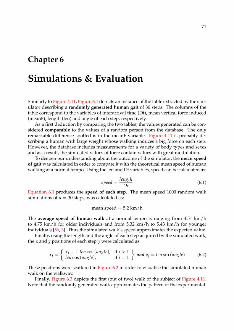
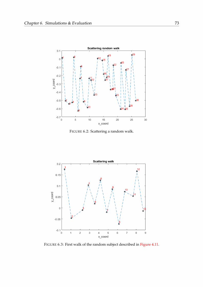
6.1 A random walk . . . . . . . . . . . . . . . . . . . . . . . . . . . . . . . . . 726.2 Scattering a random walk . . . . . . . . . . . . . . . . . . . . . . . . . . . 736.3 First walk of a random subject . . . . . . . . . . . . . . . . . . . . . . . . . 73
xi
List of Abbreviations
AIC Akaike Information CriterionASD AutoSpectral DensityBIC Bayesian Information Criterioncol Columndim DimensionDLF Dynamic Load FactorDt Interarrival TimeGM Gaussian MixtureGMM Gaussian Mixture ModelGMMs Gaussian Mixture Modelslen LengthmeanF Mean Vertical ForceND Normal Distributionpdf probability density function
xiii
Dedicated to the memory of my friend Giorgos Paterakiswho will always remind me that life is too short to defy
your dreams. He did not have enough time to pursue his. . .
1
Chapter 1
Introduction
1.1 The Pedestrian Walkway
Definition 1 The pedestrian walkway or footbridge is a type of bridge designed solely forpedestrian crossings between two points. This type of infrastructure gained prominence incontemporary architecture of the 21st century because of the growing urban expansion and thepush towards a “greener” mobility [53].
Despite the desire of the human species to overcome the obstacles of nature, there hasbeen a considerable spread of walkways dedicated exclusively to pedestrians and cy-clists only after the Second World War, following the development of the road network.This has paved the way for numerous projects of pedestrian walkways climbing overcanals, rivers or roads. The design of this type of bridge requires the development ofa sustainable approach aimed at encouraging human’s approach to the living environ-ment, even in highly urbanized tissues as well as promoting the use of bicycles andwalking not only for recreational use but also for basic needs.
Nowadays, pedestrian walkways are very widespread and are not only built forcrossing the obstacles of nature but also as a means to traverse road networks andcomplex railways safely. Figure 1.1, depicts two pedestrian walkways, designed toovercome a road and a river, respectively.
FIGURE 1.1: (a) The Knokke Footbridge in Deerlyck, Belgium - (b) TheMillennium Bridge in London, UK.
2 Chapter 1. Introduction
1.2 Issues to The Design - Vibration Serviceability
Lightness and slenderness are substantive aesthetic characteristics in the design of amodern footbridge. This is corollary given the fact that the loads these structures mustsupport are generally low (about 400-500 kg/m2).
An emblematic example of this is the London Millennium Footbridge in London,UK. It is a steel suspension footbridge crossing the River Thames, linking Banksidewith the City of London that initially opened in June 2000. On this day, thousands ofpedestrians crossed it to celebrate the grand opening and was closed for modificationsonly two days later because of unexpected lateral vibration due to resonant structuralresponse that was not adequately considered and analyzed during the design phase.For this reason, residents of London often refer to it by the nickname “Wobbly Bridge”.
These excessive vibrations are a common under-researched phenomenon that alsoapplies to other infrastructures e.g., stadiums [24] theaters [63], building floors [14, 21],and staircases [13]. In this case, the pedestrians crossed a bridge with lateral oscillationand unconsciously matched their footsteps to the sway, exacerbating it. A well-knownexample of this phenomenon is when troops march over a suspension bridge in a syn-chronized step and therefore are required to break step when crossing such a bridge.
Definition 2 Vibration serviceability analysis is in fact to ensure the human comfort whencrossing such a walkway i.e., the study of the comfort of walkways.
Consequently, the so-called vibration serviceability has become a dominant de-sign aspect to consider over the last few years and has been increasingly the focus ofresearchers worldwide [61, 54, 34, 43]. This factor is firmly linked to the possible de-formation and vibration of the structure even though these vibration phenomena gen-erally do not pose a risk to the safety of the structure. It is therefore of vital importanceto monitor and evaluate the mode of vibration to avoid discomfort situations.
The two main parameters typically used to quantitatively describe vibration re-sponse are amplitude and frequency [9]. More specifically, if the amplitude exceeds atolerance limit at the frequency of vibration, it is considered excessive i.e. the frequen-cies of vibrations induced in the bridge must be distant from the low frequencies thatare perceived by humans.
Vibration serviceability analysis can be broken down into three key componentsas depicted in Figure 1.2. These are the input (excitation source), the system (floorstructure), and the output (vibration receiver) [41, 42, 40, 50, 70]. The pedestrian is atypical receiver of vibrations in the walkway but also represents the excitation sourcethat this work will focus on, due to the induced dynamic load. Human activities such
FIGURE 1.2: Components of vibration serviceability analysis.
1.3. Thesis Contributions 3
as walking [10], jogging [45], jumping [49], and running [36] commonly create the vi-bration problems.
Over the years there have been several studies planning to establish a natural fre-quency threshold. An example of these is the NTC 2008 that concluded in the fact thata higher natural frequency to 5Hz ensures a good level of comfort to the pedestrian.However, the evaluation of vibrations induced by humans is still widely debated andpoorly understood despite the importance of vibration serviceability in the design ofthe structure. In fact, there is a wide variety of contradictory dynamic load models dueto many uncertainties associated with human walking [37]. This problem would besurpassed by an acceptable uniform model of the human walk.
1.3 Thesis Contributions
The scope of this thesis is to provide a reliable and efficient uniform model of humanwalk as well as a simulator for the sake of establishing an experimental procedureand a reference dataset for future researches taking its probabilistic nature into con-sideration. More specifically, the measurements resulting by more than 200 subjectscrossing an instrumented floor were provided and calibrated in a walk database (seechapter 5). The appropriate variables describing human gait were then extracted fromthese measurements in order to statistically describe them. Then, a statistical modeldescribing the parameters of the variable models is estimated therefore creating ouruniform model of human walk. Furthermore, a gait simulator has been developedbased on this statistical model. The output of this simulator are the n appropriate vari-ables describing a random walk of n steps.
1.4 Thesis Outline
The remainder of this thesis is structured as follows:
• In chapter 2, we introduce some basic background concerning the bipedal walk-ing as well as some key ideas used throughout the thesis. Furthermore, a defini-tion of the problem beneficial to understanding the mathematical models imple-mented is described.
• In chapter 3 we investigate the history and some related work in the field ofmodeling human-induced walking excitation.
• In chapter 4 we discuss the proposed approach, starting from the experimentalframework and the calibration of the walk database, moving on to the statisticaldescription of the variables describing human walk, then the modeling of theparameters describing these variables, and finally describing the implementationof the simulator.
• In chapter 5 we elaborate on the experimental setup and more specifically on theinstruments used for the analysis as well as the critical factors we should considerin the measurements.
4 Chapter 1. Introduction
• In chapter 6 we provide an evaluation of the simulations and the simulated re-sults.
• Finally, chapter 7 provides a conclusion for our work and suggests possible futurework.
5
Chapter 2
Background
In section 2.1, we are going to give a short introduction to the key ideas used through-out the thesis as well as present the basic concept of bipedal walking, while in sec-tion 2.2 we will present the statistical model deployed in this work.
2.1 The Bipedal Walking
2.1.1 The Walking Cycle
In most people’s eyes, walking is a simple and automatic act. However, if we focus onthe dynamics of human movement, we find that it is rather a complex mechanism. It istherefore important to understand what constitutes a complete walk cycle in this firstanalysis.
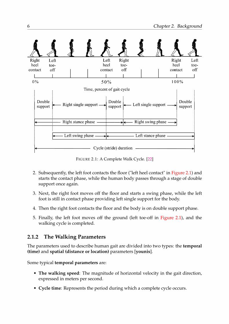
Definition 3 A complete walk cycle consists of the human body movement starting fromthe beginning of a step with one foot, up to the beginning of the next step with the same foot, asshown in Figure 2.1.
While walking, each foot passes through two phases during a single step: the swingphase and the stance (or contact) phase.
Definition 4 The swing phase refers to the period when the foot is off the floor, while thestance phase refers to the period during which the foot is in contact with the ground [4].
Concurrently, the human body goes through two stages during the walking pro-cess: the double-support and the single-support stage.
Definition 5 When the body is on the double-support stage, the feet are in contact withthe ground [32]. This stage usually comprises less than 20% of the walking cycle while as thewalking speed increases, it comprises a smaller percentage. On the contrary, the human body isat the single-support stage when one foot is in contact, while the other is off the ground [59].
A complete walk cycle can be explained as a series of consecutive events as follows[22, 20, 57, 44]:
1. The left foot is straying from the ground ("left toe-off" in Figure 2.1) in the direc-tion of walking. At the same time, the right foot provides the essential support.Thus, the left foot is in a swing phase, while the human body is in a right single-support stage.
6 Chapter 2. Background
FIGURE 2.1: A Complete Walk Cycle. [22]
2. Subsequently, the left foot contacts the floor ("left heel contact" in Figure 2.1) andstarts the contact phase, while the human body passes through a stage of doublesupport once again.
3. Next, the right foot moves off the floor and starts a swing phase, while the leftfoot is still in contact phase providing left single support for the body.
4. Then the right foot contacts the floor and the body is on double support phase.
5. Finally, the left foot moves off the ground (left toe-off in Figure 2.1), and thewalking cycle is completed.
2.1.2 The Walking Parameters
The parameters used to describe human gait are divided into two types: the temporal(time) and spatial (distance or location) parameters [younis].
Some typical temporal parameters are:
• The walking speed: The magnitude of horizontal velocity in the gait direction,expressed in meters per second.
• Cycle time: Represents the period during which a complete cycle occurs.
2.1. The Bipedal Walking 7
• Pacing rate (walking frequency): The number of steps in a specific duration,usually expressed in steps per minute or Hz [57].
Some typical spatial parameters are:
• Step length: The distance measured during a single step between both heels inthe direction of walking.
• Step width: The distance measured transversely between the two lines whichdescribe the paths taken by the right and the left foot, where these lines passthrough heel midpoints.
• Stride length: The distance measured along the gait direction between two con-secutive contacts of the same foot. It also represents the total distance traveledduring one cycle period [44].
2.1.3 The Vertical Load Induced During a Walk
Regarding the various parameters that characterize the human walking process, wecan identify the presence of two types of randomness: The intersubject and the intra-subject variability [35].
Definition 6 The intersubject variability exists because different persons will have differentkey parameters directly related to the induced forces, such as subject weight, step frequency,walking speed, and so on [68]. So, the resultant walking forces vary from person to person.However, intrasubject variability exists because an individual never repeats two identicalsteps sequentially i.e., a person produces forces that are different at each footfall [67].
A walking person causes dynamic forces that have components in three directions:the vertical the horizontal-parallel, and the horizontal-transverse to the direction ofmovement [5]. However, only the vertical force component will be addressed in thisthesis, since it has the highest magnitude of all and is by far the most significant invibration serviceability analysis.
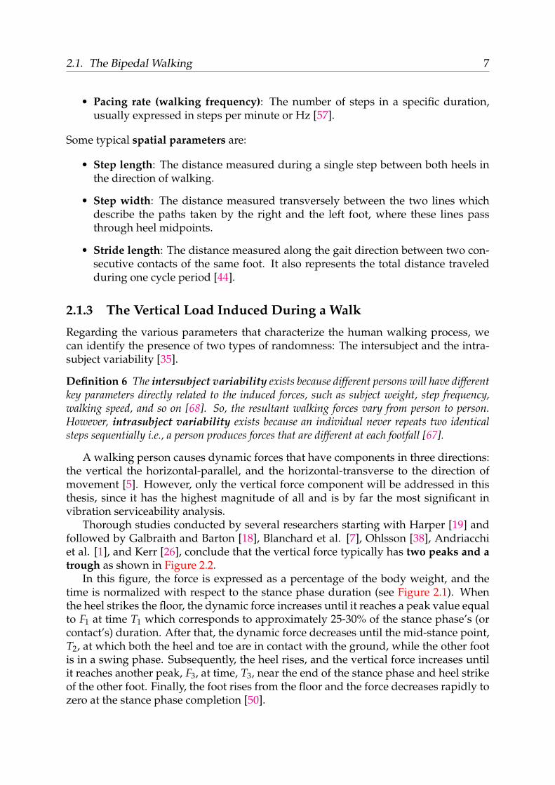
Thorough studies conducted by several researchers starting with Harper [19] andfollowed by Galbraith and Barton [18], Blanchard et al. [7], Ohlsson [38], Andriacchiet al. [1], and Kerr [26], conclude that the vertical force typically has two peaks and atrough as shown in Figure 2.2.
In this figure, the force is expressed as a percentage of the body weight, and thetime is normalized with respect to the stance phase duration (see Figure 2.1). Whenthe heel strikes the floor, the dynamic force increases until it reaches a peak value equalto F1 at time T1 which corresponds to approximately 25-30% of the stance phase’s (orcontact’s) duration. After that, the dynamic force decreases until the mid-stance point,T2, at which both the heel and toe are in contact with the ground, while the other footis in a swing phase. Subsequently, the heel rises, and the vertical force increases untilit reaches another peak, F3, at time, T3, near the end of the stance phase and heel strikeof the other foot. Finally, the foot rises from the floor and the force decreases rapidly tozero at the stance phase completion [50].
8 Chapter 2. Background
FIGURE 2.2: Vertical force induced in a single step. [50]
It was noted, however, that this graph changes considerably at different walkingspeeds. There are two main factors considered to affect the amplitude of the peakforce: the weight of the person and the frequency steps. The increase of these factorsleads to higher peak forces.
Wheeler [younis, 58] has conducted a wide-ranging study to classify different typesof human movements, arranged from slow walking to running (Figure 2.3). Each ofthese categories had a unique peak amplitude single-step dynamic force, shape, andstance period. Additionally, the author stated that different parameters such as stridelength, walking speed, contact time, peak force and step frequency are related. Forexample, increasing the step frequency leads to shortening the contact time and in-creasing the peak force.
This work will emphasize in normal tempo gaits (see Figure 2.2). Thus, runningwill not be discussed further as it is considered an extreme case of walking in terms ofmovement speed.
2.1. The Bipedal Walking 9
FIGURE 2.3: Vertical force induced for different modes of movement ac-tivity. [70]
10 Chapter 2. Background
2.2 Problem Definition
2.2.1 The Statistical Model Deployed in This Work
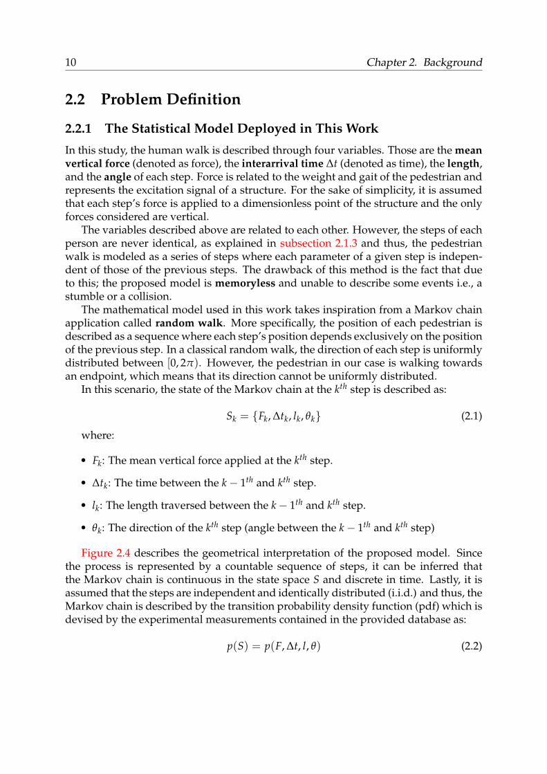
In this study, the human walk is described through four variables. Those are the meanvertical force (denoted as force), the interarrival time ∆t (denoted as time), the length,and the angle of each step. Force is related to the weight and gait of the pedestrian andrepresents the excitation signal of a structure. For the sake of simplicity, it is assumedthat each step’s force is applied to a dimensionless point of the structure and the onlyforces considered are vertical.
The variables described above are related to each other. However, the steps of eachperson are never identical, as explained in subsection 2.1.3 and thus, the pedestrianwalk is modeled as a series of steps where each parameter of a given step is indepen-dent of those of the previous steps. The drawback of this method is the fact that dueto this; the proposed model is memoryless and unable to describe some events i.e., astumble or a collision.
The mathematical model used in this work takes inspiration from a Markov chainapplication called random walk. More specifically, the position of each pedestrian isdescribed as a sequence where each step’s position depends exclusively on the positionof the previous step. In a classical random walk, the direction of each step is uniformlydistributed between [0, 2π). However, the pedestrian in our case is walking towardsan endpoint, which means that its direction cannot be uniformly distributed.
In this scenario, the state of the Markov chain at the kth step is described as:
Sk = {Fk, ∆tk, lk, θk} (2.1)
where:
• Fk: The mean vertical force applied at the kth step.
• ∆tk: The time between the k− 1th and kth step.
• lk: The length traversed between the k− 1th and kth step.
• θk: The direction of the kth step (angle between the k− 1th and kth step)
Figure 2.4 describes the geometrical interpretation of the proposed model. Sincethe process is represented by a countable sequence of steps, it can be inferred thatthe Markov chain is continuous in the state space S and discrete in time. Lastly, it isassumed that the steps are independent and identically distributed (i.i.d.) and thus, theMarkov chain is described by the transition probability density function (pdf) which isdevised by the experimental measurements contained in the provided database as:
p(S) = p(F, ∆t, l, θ) (2.2)
2.2. Problem Definition 11
FIGURE 2.4: The geometrical interpretation of the proposed model. [39]
Consequently, the correlation between the 4 variables describing the human walkwas extracted by Fornaciari [17], using some experimental measurements. More specif-ically, the correlation coefficients of distinct variables have been assessed for each stu-dent and then averaged over the number of students to devise general indications.Thus, the average matrix correlation R arises as:
• R12 = R21 = −0.33: The time-force correlation coefficient
• R13 = R31 = −0.25: The time-length correlation coefficient
• R14 = R41 = 0.02: The time-angle correlation coefficient
• R23 = R32 = 0.06: The force-length correlation coefficient
• R24 = R42 = 0.15: The force-angle correlation coefficient
• R34 = R43 = 0.08: The length-angle correlation coefficient
As it occurs, the time-force, time-length, and force-angle correlations are impor-tant whereas any other correlation can be considered negligible. We consider that for
12 Chapter 2. Background
each step, time, force, and length are correlated, while the angle variable is statisticallyindependent from the other variables. Thus, Equation 2.2 can be written as:
p(S) = p(F, ∆t, l, θ) = p(F, ∆t, l)p(θ) (2.4)
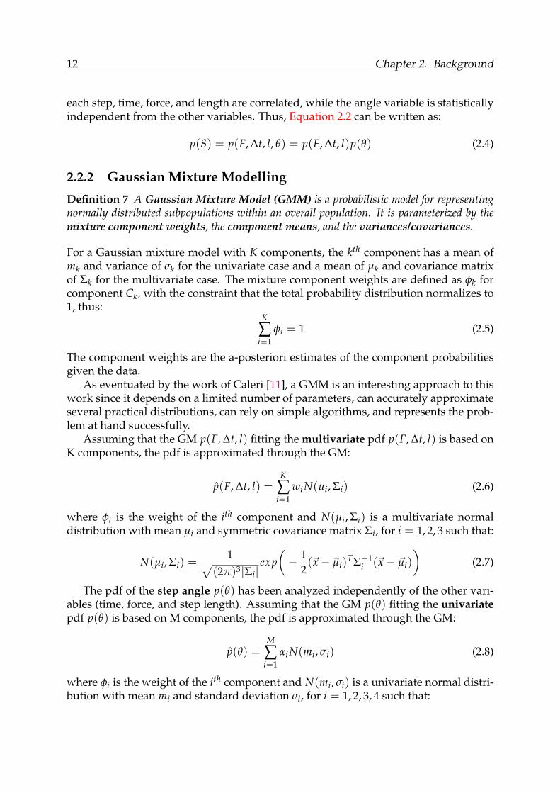
2.2.2 Gaussian Mixture Modelling
Definition 7 A Gaussian Mixture Model (GMM) is a probabilistic model for representingnormally distributed subpopulations within an overall population. It is parameterized by themixture component weights, the component means, and the variances/covariances.
For a Gaussian mixture model with K components, the kth component has a mean ofmk and variance of σk for the univariate case and a mean of µk and covariance matrixof Σk for the multivariate case. The mixture component weights are defined as φk forcomponent Ck, with the constraint that the total probability distribution normalizes to1, thus:
K
∑i=1
φi = 1 (2.5)
The component weights are the a-posteriori estimates of the component probabilitiesgiven the data.
As eventuated by the work of Caleri [11], a GMM is an interesting approach to thiswork since it depends on a limited number of parameters, can accurately approximateseveral practical distributions, can rely on simple algorithms, and represents the prob-lem at hand successfully.
Assuming that the GM p(F, ∆t, l) fitting the multivariate pdf p(F, ∆t, l) is based onK components, the pdf is approximated through the GM:
p(F, ∆t, l) =K
∑i=1
wiN(µi, Σi) (2.6)
where φi is the weight of the ith component and N(µi, Σi) is a multivariate normaldistribution with mean µi and symmetric covariance matrix Σi, for i = 1, 2, 3 such that:
N(µi, Σi) =1√
(2π)3|Σi|exp(− 1
2(~x−~µi)
TΣ−1i (~x− ~µi)
)(2.7)
The pdf of the step angle p(θ) has been analyzed independently of the other vari-ables (time, force, and step length). Assuming that the GM p(θ) fitting the univariatepdf p(θ) is based on M components, the pdf is approximated through the GM:
p(θ) =M
∑i=1
αiN(mi, σi) (2.8)
where φi is the weight of the ith component and N(mi, σi) is a univariate normal distri-bution with mean mi and standard deviation σi, for i = 1, 2, 3, 4 such that:
2.2. Problem Definition 13
N(mi, σi) =1
σi√
2πexp(− (x−mi)
2
2σ2i
)(2.9)
Concluding, the transition pdf p(S) is therefore approximated using eq: 2.4, 2.6 and2.8 as:
p(S) = p(F, ∆t, l) p(θ) =( K
∑i=1
wiN(µi, Σi)
)( M
∑i=1
αiN(mi, σi)
)(2.10)
15
Chapter 3
Related Work
In this chapter, we introduce some related work on the field of modeling human walk-ing forces. The resulted models can be used to predict vibrations during the designphase. However, this modeling presents several challenges. First, due to many param-eters being affected by the intersubject and intrasubject variability, a high variability inforce waveform shapes is presented [58] as depicted in Figure 2.3. Moreover, the dy-namic forces induced by a pedestrian are narrowband random processes that are notcompletely understood yet and thus, not accurately assessed [8].
However, several force models have been implemented by researchers and are usedduring the design phase. Two types of models are most commonly used for humanwalking excitation. These are the time-domain models that are currently more widelyused, and the frequency-domain models.
Time-domain force models are forked into two groups; the deterministic and prob-abilistic.
Definition 8 Deterministic models aim to generate a uniform force model without directlyconsidering the natural variability between people [6]. These models are based on assumptionssuch as perfect periodicity and uniformity of produced force for both feet. On the other hand,the probabilistic models consider the intersubject variability of each person i.e., each individ-ual presents unique parameters influencing the produced forces e.g., weight, tempo etc. Eachparameter is described by its pdf and hence, measured by the probability of occurrence [69].
In the remaining chapter, we first discuss about time-domain deterministic forcemodels available in the literature. Then, the frequency-domain models will be intro-duced and we conclude with some probabilistic force models that surfaced in the lastyears.
3.1 Time-Domain Deterministic Force Models
Bachmann and Ammann [5] indicated that the magnitude of human-induced vibrationdepends significantly on the ratio of walking frequency of the pedestrian and the low-est vertical natural frequency of the floor. There are two types of floors presented in theliterature according to their natural frequency: the low-frequency and high-frequencyfloors [50]. This distinction has been applied as a result of significant variations in thedynamic responses, as ascertained in several studies. The threshold frequency values
16 Chapter 3. Related Work
defining the type of floor is calculated at 9-10 Hz for floors having at least one naturalfrequency.
In the moment of writing, there is no deterministic walking force model that can beused for prediction of both low-frequency and high-frequency floor responses, due tothe different response behavior. Therefore researchers have developed different forcemodels for each.
3.1.1 Low-Frequency Force Models
Definition 9 Low-frequency floors are typically regarded as floors having at least one re-sponsive natural frequency below 9-10 Hz.
Each periodic force with a period T can be represented by a Fourier series. The verticaldynamic force induced by a pedestrian can be expressed by a summation of harmoniccomponents (i.e., Fourier series) being assumed as periodic in the time domain as:
Fp(t) = G +n
∑i=1
Gαi sin (2πi fpt− φi) (3.1)
where:
• G: The individual static weight (N).
• i: The order number of the harmonic.
• n: The number of all contributing harmonics.
• fp: The step frequency (Hz).
• φi: The phase shift of the ith harmonic (rads).
• αi: The Fourier coefficient of the ith harmonic, usually known as the dynamic loadfactor (DLF) i.e., The dynamic coefficient.
Many researchers have attempted to quantify the DLF αi for the contributing harmon-ics over the last years as it is the key to generate an accurate deterministic force model.These studies resulted in the force models included in the major footbridge designguides used today.
Blanchard et al. [7] proposed a simple deterministic force model concerning theload exerted on footbridges by a pedestrian. In this model, it is concluded that if thefundamental frequency of the walkway does not exceed 4 Hz, resonance is presentedin the first harmonic of the dynamic load with αi = 0.257 and G = 700N. If thefundamental frequency is between 4 and 5 Hz , the resonance is a result of the secondharmonic and therefore applied some reduction factors.
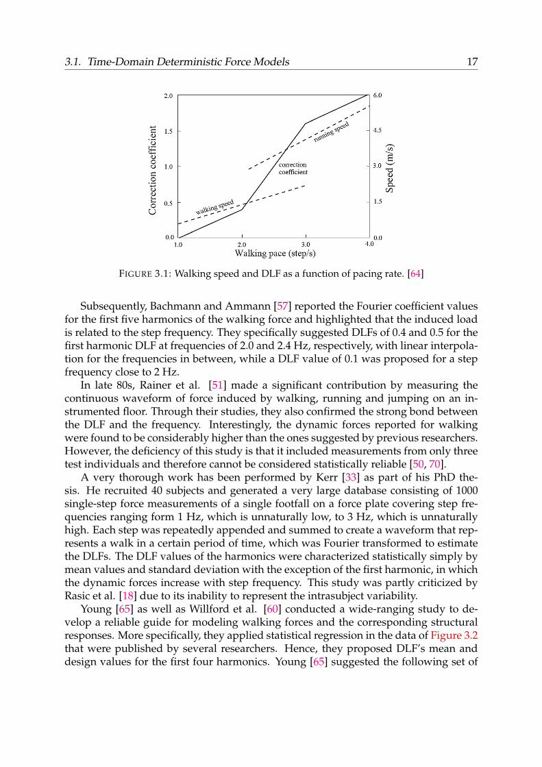
Later in 1982, Kajikawa, according to Yoneda [64], improved the previous model.More specifically, he introduced a relationship between the correction coefficient i.e.,DLF and walking pace (m/sec). The walking speed depending on step frequency wasalso added as an output of his model. His results are presented in Figure 3.1.
3.1. Time-Domain Deterministic Force Models 17
FIGURE 3.1: Walking speed and DLF as a function of pacing rate. [64]
Subsequently, Bachmann and Ammann [57] reported the Fourier coefficient valuesfor the first five harmonics of the walking force and highlighted that the induced loadis related to the step frequency. They specifically suggested DLFs of 0.4 and 0.5 for thefirst harmonic DLF at frequencies of 2.0 and 2.4 Hz, respectively, with linear interpola-tion for the frequencies in between, while a DLF value of 0.1 was proposed for a stepfrequency close to 2 Hz.
In late 80s, Rainer et al. [51] made a significant contribution by measuring thecontinuous waveform of force induced by walking, running and jumping on an in-strumented floor. Through their studies, they also confirmed the strong bond betweenthe DLF and the frequency. Interestingly, the dynamic forces reported for walkingwere found to be considerably higher than the ones suggested by previous researchers.However, the deficiency of this study is that it included measurements from only threetest individuals and therefore cannot be considered statistically reliable [50, 70].
A very thorough work has been performed by Kerr [33] as part of his PhD the-sis. He recruited 40 subjects and generated a very large database consisting of 1000single-step force measurements of a single footfall on a force plate covering step fre-quencies ranging form 1 Hz, which is unnaturally low, to 3 Hz, which is unnaturallyhigh. Each step was repeatedly appended and summed to create a waveform that rep-resents a walk in a certain period of time, which was Fourier transformed to estimatethe DLFs. The DLF values of the harmonics were characterized statistically simply bymean values and standard deviation with the exception of the first harmonic, in whichthe dynamic forces increase with step frequency. This study was partly criticized byRasic et al. [18] due to its inability to represent the intrasubject variability.
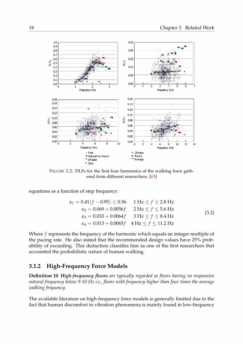
Young [65] as well as Willford et al. [60] conducted a wide-ranging study to de-velop a reliable guide for modeling walking forces and the corresponding structuralresponses. More specifically, they applied statistical regression in the data of Figure 3.2that were published by several researchers. Hence, they proposed DLF’s mean anddesign values for the first four harmonics. Young [65] suggested the following set of
18 Chapter 3. Related Work
FIGURE 3.2: DLFs for the first four harmonics of the walking force gath-ered from different researchers. [65]
1 Hz ≤ f ≤ 2.8 Hz2 Hz ≤ f ≤ 5.6 Hz3 Hz ≤ f ≤ 8.4 Hz
4 Hz ≤ f ≤ 11.2 Hz
(3.2)
Where f represents the frequency of the harmonic which equals an integer multiple ofthe pacing rate. He also stated that the recommended design values have 25% prob-ability of exceeding. This deduction classifies him as one of the first researchers thataccounted the probabilistic nature of human walking.
3.1.2 High-Frequency Force Models
Definition 10 High-frequency floors are typically regarded as floors having no responsivenatural frequency below 9-10 Hz i.e., floors with frequency higher than four times the averagewalking frequency.
The available literature on high-frequency force models is generally limited due to thefact that human discomfort in vibration phenomena is mainly found in low-frequency
3.1. Time-Domain Deterministic Force Models 19
FIGURE 3.3: Response behavior comparison of successive steps in (a) lowand (b) high frequency floors. [33]
floors. The response of these floors presents a transient or impulsive profile [33] unlikethe resonant behavior found in the response of low-frequency counterparts. Figure 3.3illustrates this difference.
In this figure it is noted that, unlike the typical low-frequency resonant responsewhich involves an accumulation in structure’s response of successive step, in high-frequency floors the vibration responses of successive steps do not build up because ofthe structural damping decaying effect. More specifically, the first heel touch producesan initial peak response followed by floor oscillating at its natural frequency with a de-caying rate associated with the damping ratio of the fundamental mode [28]. Similarly,another impulse response is generated at each subsequent step.
3.1.3 Drawbacks in Deterministic Force Modeling
Deterministic force models account for the most common approach in human walkmodeling. Thus, the reliability of those models has been extensively tested and im-portant drawbacks have been identified. First, these models usually do not considerthe inter-and intrasubject variability of human walking. Secondly, the classification offloors by their natural frequency is not considered accurate in certain circumstancese.g., a floor with a fundamental frequency close to the 9-10 Hz threshold probably
20 Chapter 3. Related Work
exhibits a mixed response and thus cannot be classified [71]. Lastly, the vibration re-sponse computed in these models is a numeral usually compared with a selected limitof vibration tolerance. This results in a binary pass or fail criterion which does notprovide enough information to make a decision in the design phase [72]. Therefore,Deterministic modeling is generally not considered very accurate or precise, leadingto wrong estimation of the floor vibration response.
3.2 Frequency Domain Force Models
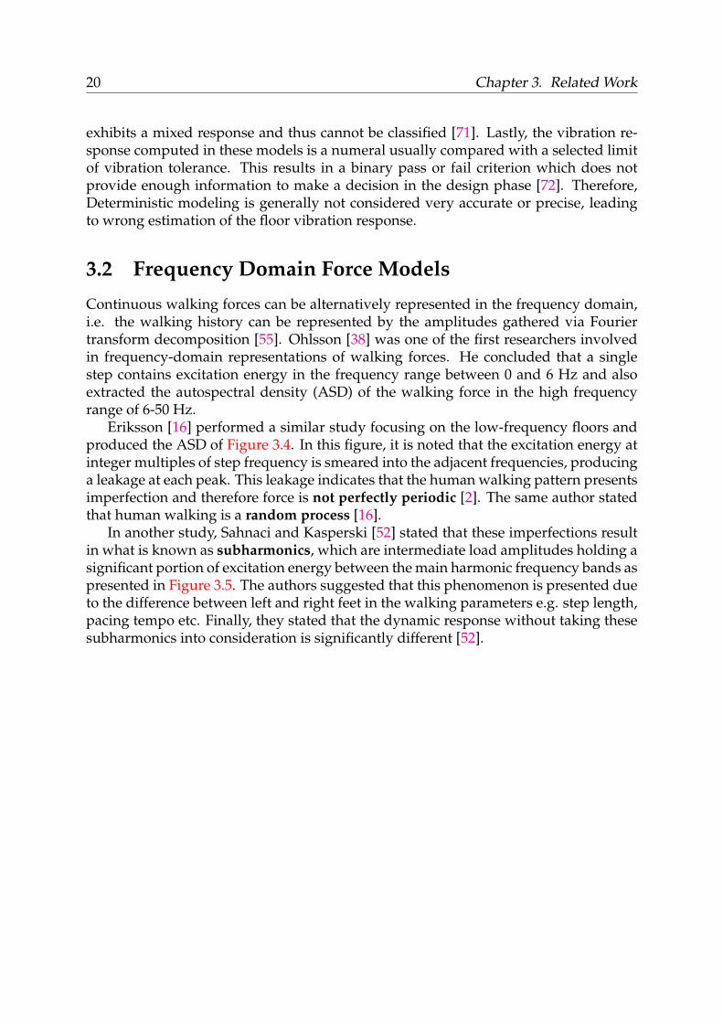
Continuous walking forces can be alternatively represented in the frequency domain,i.e. the walking history can be represented by the amplitudes gathered via Fouriertransform decomposition [55]. Ohlsson [38] was one of the first researchers involvedin frequency-domain representations of walking forces. He concluded that a singlestep contains excitation energy in the frequency range between 0 and 6 Hz and alsoextracted the autospectral density (ASD) of the walking force in the high frequencyrange of 6-50 Hz.
Eriksson [16] performed a similar study focusing on the low-frequency floors andproduced the ASD of Figure 3.4. In this figure, it is noted that the excitation energy atinteger multiples of step frequency is smeared into the adjacent frequencies, producinga leakage at each peak. This leakage indicates that the human walking pattern presentsimperfection and therefore force is not perfectly periodic [2]. The same author statedthat human walking is a random process [16].
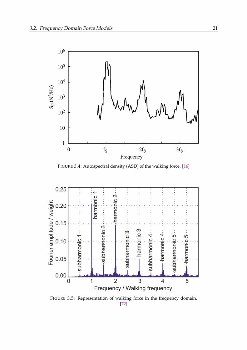
In another study, Sahnaci and Kasperski [52] stated that these imperfections resultin what is known as subharmonics, which are intermediate load amplitudes holding asignificant portion of excitation energy between the main harmonic frequency bands aspresented in Figure 3.5. The authors suggested that this phenomenon is presented dueto the difference between left and right feet in the walking parameters e.g. step length,pacing tempo etc. Finally, they stated that the dynamic response without taking thesesubharmonics into consideration is significantly different [52].
3.2. Frequency Domain Force Models 21
FIGURE 3.4: Autospectral density (ASD) of the walking force. [16]
FIGURE 3.5: Representation of walking force in the frequency domain.[72]
22 Chapter 3. Related Work
3.3 Probabilistic Force Models
The probabilistic models were developed to respond to the need for more reliable ap-proaches on the mathematical representation of the dynamic forces induced by humanwalking. These approaches take into account the intersubject and intrasubject vari-ability i.e., a large database of measurements should be provided [47]. On reflection,according to these models, the human walking is considered a random or stochas-tic process with non deterministic behavior i.e., the next state cannot be predicted bythe current state [12] and repeated experiments from the same person will be differ-ent [48]. The randomness can be expressed by the probability of the above variablesdensity function. The output of these models are not a binary value generated froma comparison on a threshold but instead, the induced response can be expressed as aprobability that will not exceed a certain value. This gives more space for engineers tomake a decision on vibration serviceability [31].
3.3.1 Step Frequency of Probabilistic Force Models
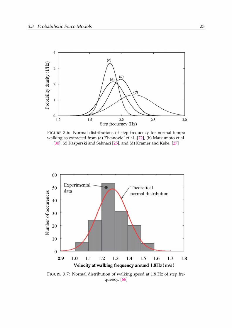
There is a notable difference between step properties from several studies in the lit-erature [72, 30, 25, 27]. Figure 3.6 depicts the normal distributions of step frequencyfor normal tempo walking as extracted in several researches. These differences occurbecause of the fact that step properties have been proven to depend on multiple fac-tors such as gender, nation, culture [66, 62] and the environment [23]. Therefore, Racicet al. [50] suggested that in order to perform a reliable statistical analysis of walkingparameters, a random sample of people from different genders, nations, and culturesshould be collected.
Using statistical analysis, Zivanovic [66] noted that walking speed follows a nor-mal distribution pattern, as illustrated in Figure 3.7. In this figure, the step frequencyis adjusted at 1.8 Hz as this is the mean value of the normal probability distributiondescribing step frequency introduced by Pachi and Ji [23].
3.3.2 Probabilistic Force Models Available in the Literature
Ebrahimpour et al. [15] performed one of the first attempts to include the randomnessinto human induced walking forces. In the study about the dynamic loads induced bycrowds of pedestrians, they achieved a model that can be used to determine the firstharmonic DLF given the step frequency and the number of people (Figure 3.8). How-ever, their model is not comprehensive and cannot be applied to predict the vibrationresponse.
Later, Zivanovic [66] implemented a framework to predict the vertical response ofa walkway excited by a single pedestrian. This was performed by first performing astatistical analysis on the walking parameters and finally extracting the pdfs of theseparameters in order to calculate the cumulative probability that the vibration response
3.3. Probabilistic Force Models 23
FIGURE 3.6: Normal distributions of step frequency for normal tempowalking as extracted from (a) Zivanovic´ et al. [72], (b) Matsumoto et al.
[30], (c) Kasperski and Sahnaci [25], and (d) Kramer and Kebe. [27]
FIGURE 3.7: Normal distribution of walking speed at 1.8 Hz of step fre-quency. [66]
24 Chapter 3. Related Work
FIGURE 3.8: DLFs of the first harmonic as a function of the number ofpersons and step frequency. [15]
does not exceed a specified threshold. This framework however is bounded for foot-bridges presenting light traffic and only the first mode of vibrations is counted. Nev-ertheless, it is concluded that the first step to develop a reliable probabilistic model isto represent the single pedestrian excitation.
Consequently, Zivanovic´et al. [72] have extended this model to include the sub-harmonics appearing in the frequency domain, unlike previous models considering themain harmonics only, as shown in Figure 3.9. The authors have accounted the inter-subject variability using the pdfs of the variables describing the human walk as well asthe intrasubject variability via the phase angle, which was represented in the frequencydomain with a random pattern uniformly distributed between (−π, π). However, dueto the lack of measurement database for subharmonics, the corresponding amplitudeswere included as a function of the first harmonic’s DLF. The accuracy of this modelwas proved to be adequate based on the experimental results.
Another model was introduced by Racic and Brownjohn [46]. This model emergedby an experimental campaign of 824 steps from about 80 subject of different physicalcharacteristics. In this work, the authors categorized the walking signals into 20 clus-ters according to the pacing rate, each of 0.1 Hz, as depicted in Figure 3.10. Finally,they explained an algorithm for generating the walking force signals. However, theproposed modeling approach is numerically complicated thus making it impracticalfor the design engineers as the current techniques require simple calculations.
3.3. Probabilistic Force Models 25
FIGURE 3.9: (a) 80-step walking force time history for a single pedestrian,(b) DLFs for the main harmonics and subharmonics in the frequency do-main, (c) phase angle of forces in Fourier spectrum and (d) period of walk-
ing steps. [72]
FIGURE 3.10: Categorization of walking force signals based on pacingrate. [46]
27
Chapter 4
Proposed Approach
In this chapter, we introduce the proposed approach to the problem. More specifically,in the first phase, we try to develop a uniform model of human walk. Therefore,the variables characterizing the walk of each subject in the database are modeled andthen the parameters of the resulted models are fitted into new models to describe themuniformly as illustrated in the brief modeling plan of Figure 4.1.
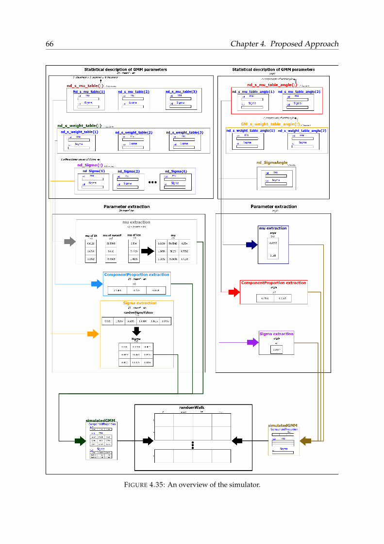
In second phase, a simulator of random human walk was implemented based onour models for the sake of establishing an experimental procedure as well as a referencedataset for future researches. Technically, this simulator uses the models describing theparameters, developed in the first phase, and generates random parameters. These pa-rameters will be fitted into a new model that constitutes our simulator. This procedureis depicted in the brief simulation plan of Figure 4.2.
The aforementioned are described analytically in the following sections.
28 Chapter 4. Proposed Approach
FIGURE 4.1: A brief modeling plan.
FIGURE 4.2: A brief simulation plan.
4.1. Experimental Framework 29
4.1 Experimental Framework
4.1.1 Database Properties
The database used for the modeling of human walk consists of valid measurementsfor more than 200 pedestrians in a variety of physical characteristics. More specifi-cally, each subject was asked to cross a 10m2 plane walkway twice at a normal tempo.The equipment used to conduct the experiments included 10 plates along with theappropriate force sensors that occupy 1m2 each, as described in chapter 5.
Subsequently, the database provided for the analysis was in the form of a cell tableof 229 rows (subjects) and differed number of columns depending on the steps mea-sured for each individual (minimum is 21 while maximum is 32 steps) for a samplingfrequency of 50Hz. It is important to note that each subject (row) includes measure-ments of both walks for the specific individual e.g. if the first cross consisted of 14steps and the second of 13, columns 1-14 include the measurements for the first walkand columns 15-27 include those of the second. Furthermore, some of the 229 rowsare empty i.e., do not contain any measurements and as a result, will be consideredinvalid for the analysis.
Considering the subject (row) index as i and the step (column) index as j, eachcell {i, j} in the database matrix includes measured information about force, time andposition on the plane for the ith pedestrian at the jth step.
Thus, database cell {i,j}.time is an array of measured times that step j lastedcorresponding to the forces induced during this step which are found on {i,j}.force(maximum 70 measurements for each step). The time measurements were extractedby a timer used in the experimental procedure. Consequently, {i,j}.force is an ar-ray of vertical forces induced during each step corresponding to the time array andmeasured in Newtons.
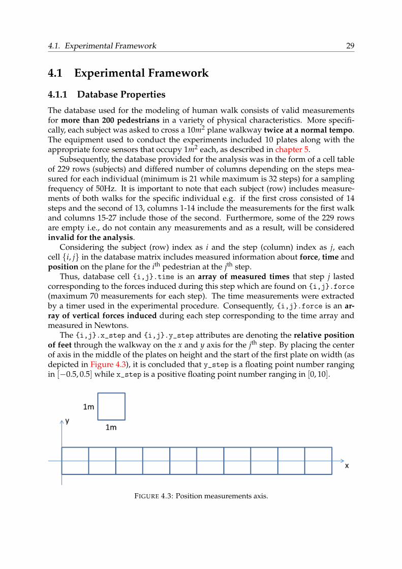
The {i,j}.x_step and {i,j}.y_step attributes are denoting the relative positionof feet through the walkway on the x and y axis for the jth step. By placing the centerof axis in the middle of the plates on height and the start of the first plate on width (asdepicted in Figure 4.3), it is concluded that y_step is a floating point number rangingin [−0.5, 0.5] while x_step is a positive floating point number ranging in [0, 10].
FIGURE 4.3: Position measurements axis.
30 Chapter 4. Proposed Approach
FIGURE 4.4: Simplified form of the initial database.
Finally, the first column of each pedestrian {i, 1}, includes some extra measurementinformation. More specifically, {i,1}.x and {i,1}.y contain the information aboutwhich points of each plate came in contact through the path, {i,1}.Ptot representsthe sum of measurements acquired by all the force sensors beneath the instrumentedfloor and {i,1}.P_div collects the signals acquired by all the force sensors i.e., 10 platesand 4 sensors installed on each plate for a total of 40 measurements at each clock cycle.Those are raw data and will not be used on this work.
Figure 4.4 depicts a simplified form of the initial database which was providedfor the analysis. In this example, it is obvious that each subject differs at number ofsteps performed on the 2 walks. Also, some subjects do not contain any measurements(subject 228 in this example) and ascribed to this, are considered invalid.
4.1.2 Database Analysis
The initial database, as described in subsection 4.1.1, needed some modifications inorder to satisfy the requirements of the modelling. First of all, it needed to containvalid measurements only, but also force-time arrays contained in each cell are requiredto have the same indices on all cells on the basis that the measurements would later
4.1. Experimental Framework 31
FIGURE 4.5: Simplified form of the modified database.
be unified in tables for easier and more effective use. For this purpose, a "clear-out" isperformed.
Initially, the subjects (rows) with empty measurements were identified and deleted.As a result, the database now contains measurements for 215 subjects as opposed tothe 229 initial subjects. This modification is depicted in Figure 4.5. Furthermore, theforce values are always be positive but due to some errors during the measurementprocedure, this was not the case on some occasions. Hence, force measurements withnegative values as well as the corresponding time values have been replaced with nanvalues in order to practically remove them from the database.
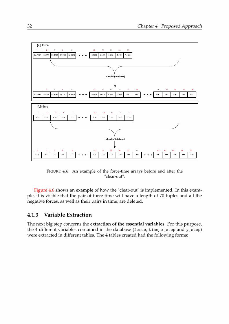
Finally, the force-time arrays were further modified to have the same indices onall cells as depicted in Figure 4.6. These arrays initially had different indices on eachcell but mutually the same. These modifications were crucial as a unified table wouldbe needed for each of those variables. To do so, the maximum force-time array in-dices in the database were identified and each array was modified to fit these indicesby adding nan values to the bottom of the array until the indices reach this maximumnumber. More specifically, the maximum array indices were calculated as 70 and there-fore, each force-time array contains up to 70 measurements but always has 70 tuples.
32 Chapter 4. Proposed Approach
FIGURE 4.6: An example of the force-time arrays before and after the"clear-out".
Figure 4.6 shows an example of how the "clear-out" is implemented. In this exam-ple, it is visible that the pair of force-time will have a length of 70 tuples and all thenegative forces, as well as their pairs in time, are deleted.
4.1.3 Variable Extraction
The next big step concerns the extraction of the essential variables. For this purpose,the 4 different variables contained in the database (force, time, x_step and y_step)were extracted in different tables. The 4 tables created had the following forms:
4.1. Experimental Framework 33
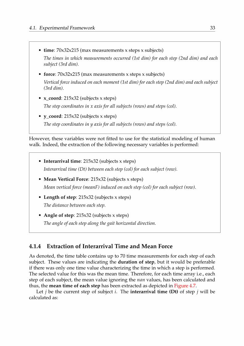
• time: 70x32x215 (max measurements x steps x subjects)
The times in which measurements occurred (1st dim) for each step (2nd dim) and eachsubject (3rd dim).
• force: 70x32x215 (max measurements x steps x subjects)
Vertical force induced on each moment (1st dim) for each step (2nd dim) and each subject(3rd dim).
• x_coord: 215x32 (subjects x steps)
The step coordinates in x axis for all subjects (rows) and steps (col).
• y_coord: 215x32 (subjects x steps)
The step coordinates in y axis for all subjects (rows) and steps (col).
However, these variables were not fitted to use for the statistical modeling of humanwalk. Indeed, the extraction of the following necessary variables is performed:
• Interarrival time: 215x32 (subjects x steps)
Interarrival time (Dt) between each step (col) for each subject (row).
• Mean Vertical Force: 215x32 (subjects x steps)
Mean vertical force (meanF) induced on each step (col) for each subject (row).
• Length of step: 215x32 (subjects x steps)
The distance between each step.
• Angle of step: 215x32 (subjects x steps)
The angle of each step along the gait horizontal direction.
4.1.4 Extraction of Interarrival Time and Mean Force
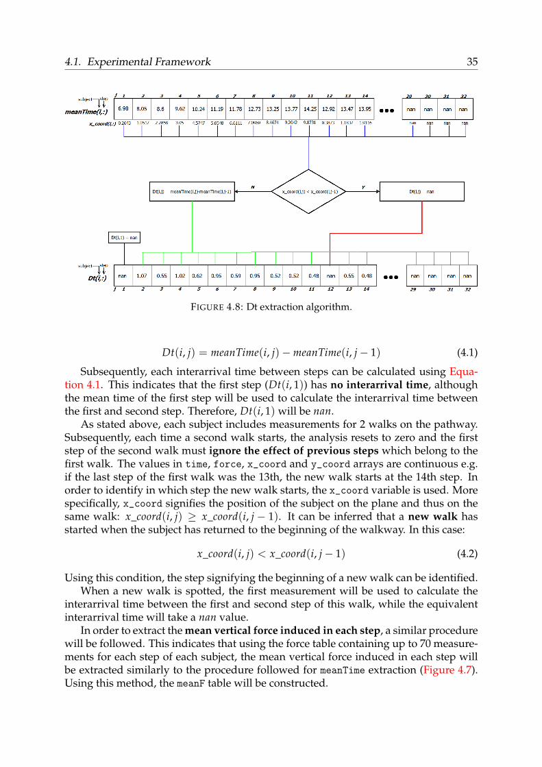
As denoted, the time table contains up to 70 time measurements for each step of eachsubject. These values are indicating the duration of step, but it would be preferableif there was only one time value characterizing the time in which a step is performed.The selected value for this was the mean time. Therefore, for each time array i.e., eachstep of each subject, the mean value ignoring the nan values, has been calculated andthus, the mean time of each step has been extracted as depicted in Figure 4.7.
Let j be the current step of subject i. The interarrival time (Dt) of step j will becalculated as:
34 Chapter 4. Proposed Approach
FIGURE 4.7: Construction of meanTime table.
4.1. Experimental Framework 35
FIGURE 4.8: Dt extraction algorithm.
Dt(i, j) = meanTime(i, j)−meanTime(i, j− 1) (4.1)
Subsequently, each interarrival time between steps can be calculated using Equa-tion 4.1. This indicates that the first step (Dt(i, 1)) has no interarrival time, althoughthe mean time of the first step will be used to calculate the interarrival time betweenthe first and second step. Therefore, Dt(i, 1) will be nan.
As stated above, each subject includes measurements for 2 walks on the pathway.Subsequently, each time a second walk starts, the analysis resets to zero and the firststep of the second walk must ignore the effect of previous steps which belong to thefirst walk. The values in time, force, x_coord and y_coord arrays are continuous e.g.if the last step of the first walk was the 13th, the new walk starts at the 14th step. Inorder to identify in which step the new walk starts, the x_coord variable is used. Morespecifically, x_coord signifies the position of the subject on the plane and thus on thesame walk: x_coord(i, j) ≥ x_coord(i, j − 1). It can be inferred that a new walk hasstarted when the subject has returned to the beginning of the walkway. In this case:
x_coord(i, j) < x_coord(i, j− 1) (4.2)
Using this condition, the step signifying the beginning of a new walk can be identified.When a new walk is spotted, the first measurement will be used to calculate the
interarrival time between the first and second step of this walk, while the equivalentinterarrival time will take a nan value.
In order to extract the mean vertical force induced in each step, a similar procedurewill be followed. This indicates that using the force table containing up to 70 measure-ments for each step of each subject, the mean vertical force induced in each step willbe extracted similarly to the procedure followed for meanTime extraction (Figure 4.7).Using this method, the meanF table will be constructed.
36 Chapter 4. Proposed Approach
FIGURE 4.9: Shifting the nans to the end of each row.
However, in order to keep the necessary correspondence between Dt and meanF,the values of the first step of each walk will be erased. In other words, in whichevertuples Dt has the value of nan, meanF will get the nan value as well. Finally, the nanvalues of Dt and meanF tables are shifted to the end of each row as shown in Figure 4.9.
4.1.5 Extraction of Length and Angle
Concerning the extraction of length and angle, the x_coord and y_coord tables areused. More specifically, the length can be calculated as the Euclidean distance betweenone step and the next, while the angle is the arctangent of the traversed x and y.
This indicates that the first step of each walk will be used to calculate the lengthand angle between the first and second step. Nevertheless, there are no values corre-sponding to these steps and thus, their values will be ignored and shifted to the end ofeach row following the procedure described for Dt and meanF.
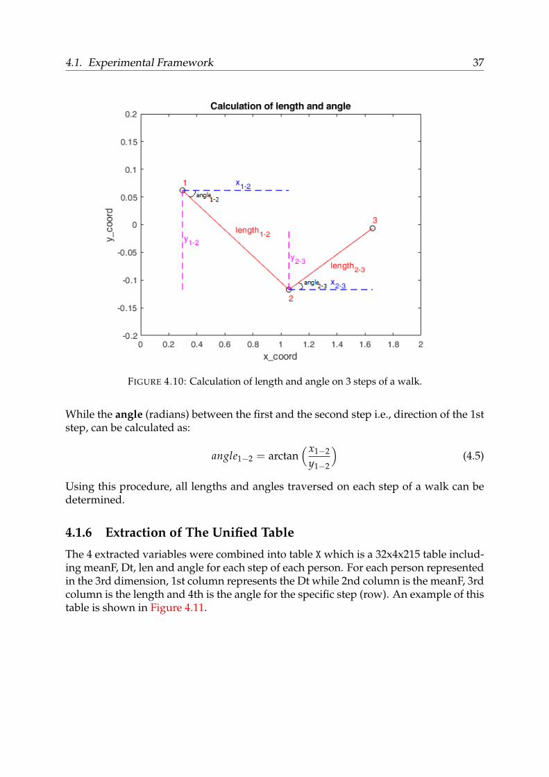
Figure 4.10 illustrates the way length and angle are calculated. In this example, 3consecutive steps of a subject are depicted as circles in the x and y domain based on thecoordinates taken by the x_coord and y_coord tables. x1−2 and y1−2 are the traversedx and y distances between the first and second step, respectively, and thus:
x1−2 = x2 − x1 and y1−2 = y2 − y1 (4.3)
The distance between the first and the second step i.e., length of the 1st step, can becalculated using the Euclidean distance as:
length1−2 =√
x21−2 + y2
1−2 (4.4)
4.1. Experimental Framework 37
FIGURE 4.10: Calculation of length and angle on 3 steps of a walk.
While the angle (radians) between the first and the second step i.e., direction of the 1ststep, can be calculated as:
angle1−2 = arctan(x1−2
y1−2
)(4.5)
Using this procedure, all lengths and angles traversed on each step of a walk can bedetermined.
4.1.6 Extraction of The Unified Table
The 4 extracted variables were combined into table X which is a 32x4x215 table includ-ing meanF, Dt, len and angle for each step of each person. For each person representedin the 3rd dimension, 1st column represents the Dt while 2nd column is the meanF, 3rdcolumn is the length and 4th is the angle for the specific step (row). An example of thistable is shown in Figure 4.11.
38 Chapter 4. Proposed Approach
FIGURE 4.11: The form of a random pedestrian’s unified table X.
4.2. Variable Modeling 39
4.2 Variable Modeling
Fornaciari [17] has concluded that the angle does not present any correlation with theother three random variables (see subsection 2.2.1). Based on these results, it is clearthat the mathematical model used to describe the human walk will need to encounterthe angle variable separately than Dt, meanF and len. Using this deduction, Caleri [11]tried to fit a variety of distributions to identify which describes the process of humanwalk better (see subsection 2.2.2). He concluded that Gaussian Mixture Models werea good approach in most cases.
Based on this deduction, we decided to fit two GMMs on each subject i.e., a mul-tivariate describing the 3 correlated variables and a univariate describing the angle.This resulted to a total of 430 GMMs to model the variables of walk. However, a deci-sion on the number of components to use on these GMMs is considered essential.
4.2.1 Estimation of GMM Components
In this section we will present the procedure adopted to estimate the number of com-ponents used in the multivariate GMMs describing the three correlated variables (Dt,meanF and len). A similar procedure will be used for the estimation on all followingGMMs. More specifically, the goal is to estimate the optimal number of GMM com-ponents i.e., the resulting GMMs should describe the variables accurately as well asminimize the complexity. The AIC and BIC criteria were used for this decision.
It must be noted here that the SharedCovariance property of the GMM has beenset to true for all GMM fits described in this work, as setting it to false would notgenerate the GMM distribution due to the ill-conditioning of the covariance matrix.Also, the number of iterations performed by the fitting algorithm has been set to 1500.
Definition 11 The Bayesian information criterion (BIC) is a criterion for model selectionamong a finite set of models. It is based, in part, on the likelihood function, and it is closelyrelated to the Akaike information criterion (AIC).
When fitting models, it is possible to increase the likelihood by adding parameters,but doing so may result in overfitting. The BIC resolves this problem by introducing apenalty term for the number of parameters in the model. The penalty term is larger inBIC than in AIC.Mathematically BIC can be defined as:
BIC = ln(n)k− 2ln(L) (4.6)
While AIC can be defined as:
AIC = 2k− 2ln(L) (4.7)
Where:
• L: The maximized value of the likelihood function of the model.
40 Chapter 4. Proposed Approach
• n: The number of data points.
• k: the number of parameters to be estimated.
A lower AIC and BIC value indicates lower penalty terms hence a better model.Though AIC and BIC are derived from a different perspective, they are closely re-
lated. Apparently, the only difference is that BIC considers the number of observationsin the formula, which AIC does not.
4.2.1.1 The Default Index Method
The default method for the estimation of the optimal number of GMM componentsdescribing the three variables (Dt, meanF, len), is based on fitting the GMMs using avariety of components. More specifically, each GMM is fitted using 1-15 components.In each selection, the AIC and BIC scores are extracted. The number of componentsthat achieve the lowest score describe the best model.
Figure 4.12 depicts the AIC and BIC values for a variety of components on 11 pedes-trians. As observed, in most cases a bigger number of components leads to smallerscores. Consequently, the penalty AIC/BIC criteria give to complex models leads tooverfitting. This phenomenon probably occurs due to the impact of noise in the data.More specifically, the data have an abnormal distribution which leads to overfitting themodel to cover these values. Thus, this method is not optimal for the estimation as itleads to bigger complexity.
4.2.1.2 Exploring a Solution
Estimating the number of components can be regarded as an important factor in theaccuracy of our model. Thus, it is significant to explore other techniques that willaid on this quest. By observing Figure 4.12 we notice that the curve follows differentslopes in different part of it. Hence, there is no need to find a global minimum of theAIC/BIC score and for this reason, we decided to check where the AIC/BIC curvechange slope is big i.e., detect the most drastic change of the AIC/BIC index, as tosignify a change of performance. This should denote the number of components thatdrastically impacts the fit and therefore could be accepted as a descent point of focus.This point will offer better optimality - complexity payoff in the GMMs.
It is important to note that each time a GMM is fitted on data the produced resultswill defer i.e., multiple GMMs fitted on the same data with the same number of compo-nents will produce different results. Therefore, in the selected method, we repeat thesame procedure in order to get more representative results. In this case we abstractlyrepeat the fittings 12 times in each case. Thus, we decided to adopt the following tech-nique:
• First, a GMM is fitted on the data and the AIC/BIC scores on 1-15 componentsare extracted.
• Then, a mean index evaluation diagram is created from all the 12 repetitions i.e.,the mean AIC/BIC scores of the 12 GMMs are calculated for each point (compo-nent).
4.2. Variable Modeling 41
FIGURE 4.12: AIC and BIC values of GMMs varying components fitted on11 pedestrians.
42 Chapter 4. Proposed Approach
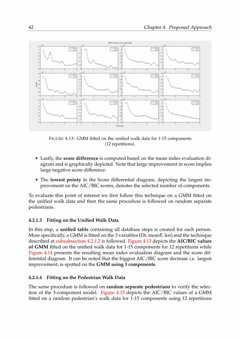
FIGURE 4.13: GMM fitted on the unified walk data for 1-15 components(12 repetitions).
• Lastly, the score difference is computed based on the mean index evaluation di-agram and is graphically depicted. Note that large improvement in score implieslarge negative score difference.
• The lowest pointy in the Score differential diagram, depicting the largest im-provement on the AIC/BIC scores, denotes the selected number of components.
To evaluate this point of interest we first follow this technique on a GMM fitted onthe unified walk data and then the same procedure is followed on random separatepedestrians.
4.2.1.3 Fitting on the Unified Walk Data
In this step, a unified table containing all database steps is created for each person.More specifically, a GMM is fitted on the 3 variables (Dt, meanF, len) and the techniquedescribed at subsubsection 4.2.1.2 is followed. Figure 4.13 depicts the AIC/BIC valuesof GMM fitted on the unified walk data for 1-15 components for 12 repetitions whileFigure 4.14 presents the resulting mean index evaluation diagram and the score dif-ferential diagram. It can be noted that the biggest AIC/BIC score decrease i.e. largestimprovement, is spotted on the GMM using 3 components.
4.2.1.4 Fitting on the Pedestrian Walk Data
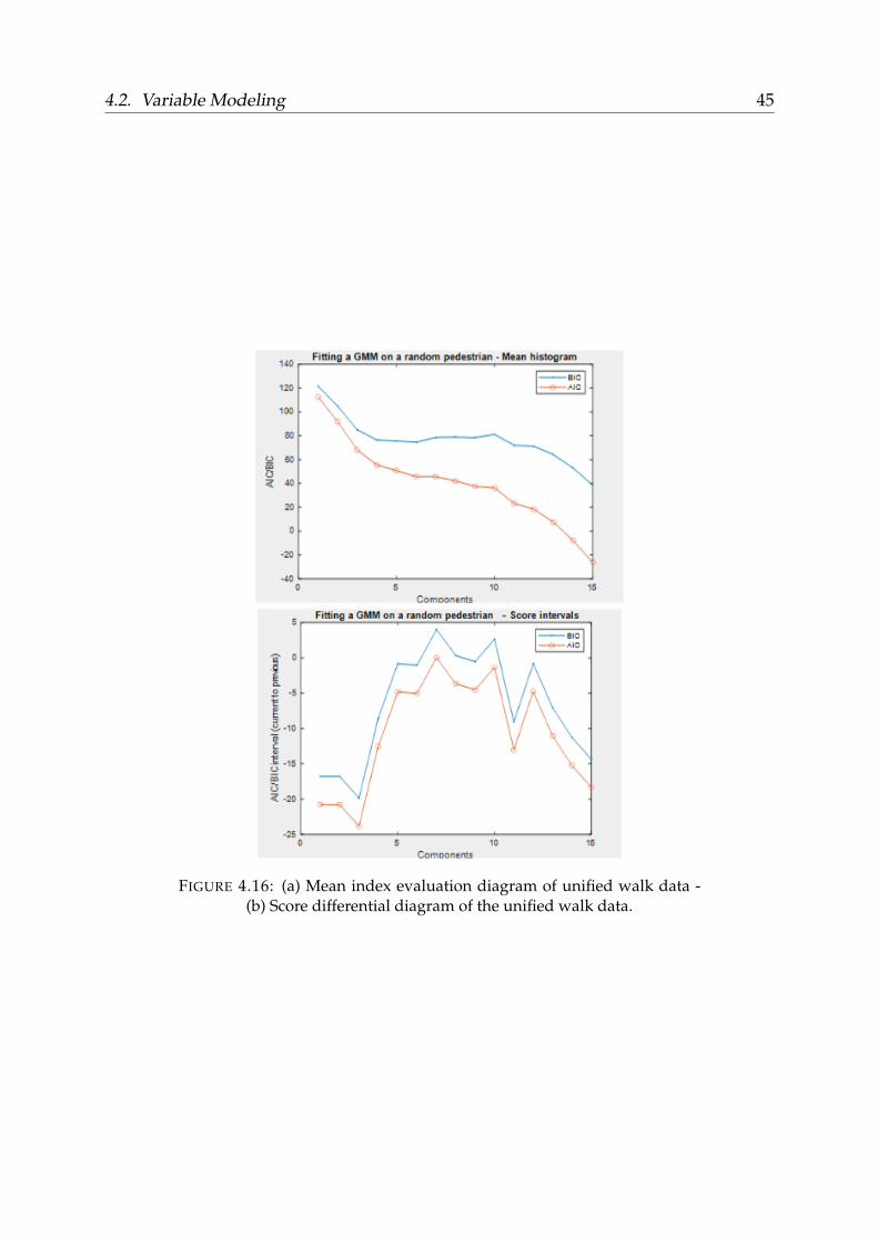
The same procedure is followed on random separate pedestrians to verify the selec-tion of the 3-component model. Figure 4.15 depicts the AIC/BIC values of a GMMfitted on a random pedestrian’s walk data for 1-15 components using 12 repetitions
4.2. Variable Modeling 43
FIGURE 4.14: (a) Mean index evaluation diagram of unified walk data -(b) Score differential diagram of the unified walk data.
44 Chapter 4. Proposed Approach
FIGURE 4.15: GMM fitted on a random pedestrian’s data for 1-15 compo-nents (12 repetitions).
while Figure 4.16 presents the resulting mean index evaluation diagram and the scoredifferential diagram.
The results obtained verify that the 3-component GMM offers better payoff andthus we decided to use 3 components on the fitting of the multivariate model describ-ing Dt, meanF and len. These experiments were repeated on many random pedestrianswith similar results in most cases.
Note: The procedures described in subsection 4.2.1 are followed before every GMM fit reportedin this work.
4.2.2 Distribution Fitting
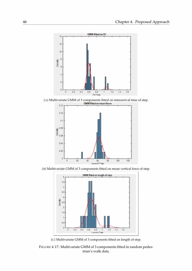
Fitting of the 3-component multivariate GMM describing Dt, meanF and len in therespective walking data is performed in this section. Figure 4.17 depicts this fittingfor a random pedestrian on each variable. More specifically, Figure 4.17a presents thedata fitted on the interarrival time of step, while Figure 4.17b and Figure 4.17c depictsthe fitting on the mean vertical force induced in each step and the length traversed,respectively.
We note that the fittings presented in this figure are performed accurately on thesignificant parts of data while ignoring the values with low density. In this manner,we consider these values as outliers or noise in the data and we ignore them in themodeling while simultaneously achieving a low complexity.
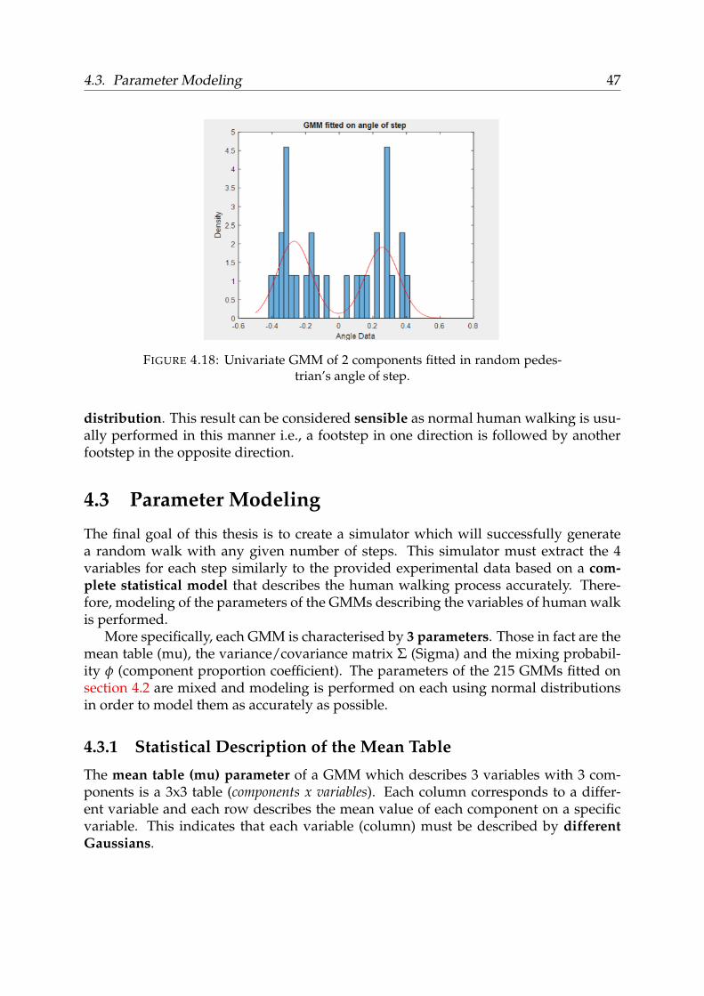
Using the technique introduced at subsection 4.2.1, we decided to use a 2-componentGMM for the modeling of data describing the angle of step for each pedestrian. Fig-ure 4.18 depicts the fitting on the angle of step of a random pedestrian’s data. It canbe inferred that the 2-component GMM presents 2 curves in the form of a bivariate
4.2. Variable Modeling 45
FIGURE 4.16: (a) Mean index evaluation diagram of unified walk data -(b) Score differential diagram of the unified walk data.
46 Chapter 4. Proposed Approach
(A) Multivariate GMM of 3 components fitted on interarrival time of step.
(B) Multivariate GMM of 3 components fitted on mean vertical force of step.
(C) Multivariate GMM of 3 components fitted on length of step.
FIGURE 4.17: Multivariate GMM of 3 components fitted in random pedes-trian’s walk data.
4.3. Parameter Modeling 47
FIGURE 4.18: Univariate GMM of 2 components fitted in random pedes-trian’s angle of step.
distribution. This result can be considered sensible as normal human walking is usu-ally performed in this manner i.e., a footstep in one direction is followed by anotherfootstep in the opposite direction.
4.3 Parameter Modeling
The final goal of this thesis is to create a simulator which will successfully generatea random walk with any given number of steps. This simulator must extract the 4variables for each step similarly to the provided experimental data based on a com-plete statistical model that describes the human walking process accurately. There-fore, modeling of the parameters of the GMMs describing the variables of human walkis performed.
More specifically, each GMM is characterised by 3 parameters. Those in fact are themean table (mu), the variance/covariance matrix Σ (Sigma) and the mixing probabil-ity φ (component proportion coefficient). The parameters of the 215 GMMs fitted onsection 4.2 are mixed and modeling is performed on each using normal distributionsin order to model them as accurately as possible.
4.3.1 Statistical Description of the Mean Table
The mean table (mu) parameter of a GMM which describes 3 variables with 3 com-ponents is a 3x3 table (components x variables). Each column corresponds to a differ-ent variable and each row describes the mean value of each component on a specificvariable. This indicates that each variable (column) must be described by differentGaussians.
48 Chapter 4. Proposed Approach
The procedure followed for the most accurate statistical description of the mu ofeach variable, will be illustrated using an example. The tables depicted in Figure 4.21are an example of the mean tables used as parameters on each subject’s GMM.
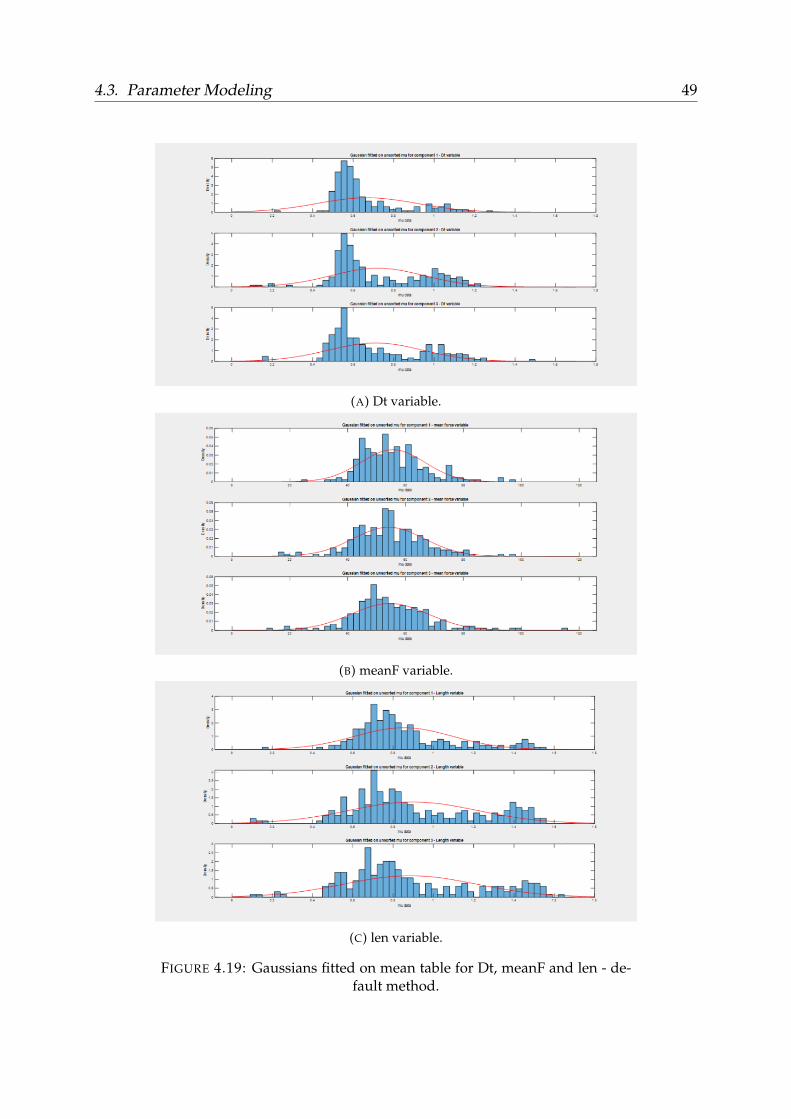
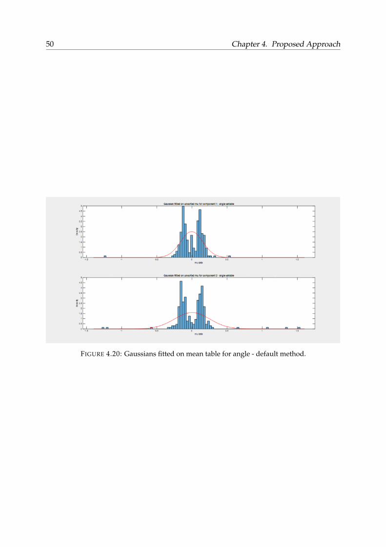
Our approach models each of the 3 mean values describing each variable (Dt, meanF,len) separately e.g., each of the first column’s values corresponds to the mean value ofeach GMM component describing Dt. The first step to this approach is to take the 3 or2 values of each mean table that correspond to the specific variable and put them ina unified 215x3 or 215x2 table (subjects x components) for the multivariate (Dt, meanF,len) or univariate (angle) case respectively. We initially fitted a Gaussian on each ofthe mean values of the variable. However, the resulted models ignore the low valueswhich play a significant role in the mean table as depicted in Figure 4.19 for Dt, meanF,len and Figure 4.20 for angle.
To counteract this problem, we decided to model the values based on their ampli-tude i.e., separate the mean values in different modes with varying amplitudes. Forinstance, the distribution of Dt has 3 modes, leading to 3 mean values in each testcase with varying amplitudes. Thus, we organize 3 groups of test model parameters;large, medium and small. This is conducted by sorting each variable’s mean values inascending order as presented in Figure 4.21.
Consequently, each sorted element is then distributed in a corresponding array thuscreating 3 arrays containing the mu values of each GMM in ascending order. Lastly,a Gaussian is fitted in each array thus creating a model of 3 normal distributions de-scribing the mean values of Dt. The aforementioned are depicted in Figure 4.22. Thesame procedure is followed for the other 3 variables noting that the angle variable isdescribed by a model of 2 normal distributions.
In summary, the modeling of the GMMs’ mean table parameter starts at unificationand ascending sorting of the mean values. Then, a Gaussian is fitted for each compo-nent of each variable. Therefore, Dt, meanF and len are statistically described using3 normal distributions on each variable while 2 normal distributions are used for theangle resulting in a total of 11 normal distributions.
Figure 4.23 depicts the Gaussians fitted on Dt, meanF and len. In this figure wenotice that the modeling takes all modes into consideration while the same applies forFigure 4.24 depicting the Gaussians fitted on angle. Moreover, the bivariate nature ofangle is modeled using this procedure.
4.3. Parameter Modeling 49
(A) Dt variable.
(B) meanF variable.
(C) len variable.
FIGURE 4.19: Gaussians fitted on mean table for Dt, meanF and len - de-fault method.
50 Chapter 4. Proposed Approach
FIGURE 4.20: Gaussians fitted on mean table for angle - default method.
4.3. Parameter Modeling 51
FIGURE 4.21: Mean table’s modeling logic for Dt variable - part 1.
52 Chapter 4. Proposed Approach
FIGURE 4.22: Mean table’s modeling logic for Dt variable - part 2.
4.3. Parameter Modeling 53
(A) Dt variable.
(B) meanF variable.
(C) len variable.
FIGURE 4.23: Gaussians fitted on mean table for Dt, meanF and len.
54 Chapter 4. Proposed Approach
FIGURE 4.24: Gaussians fitted on mean table for angle.
4.3. Parameter Modeling 55
4.3.2 Statistical Description of the Mixing Probability (ComponentProportion Coefficients)
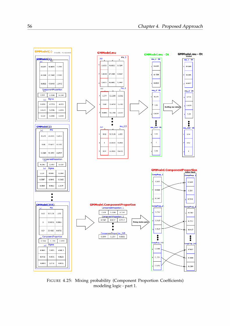
The mixing probability parameter (Component Proportion Coefficients) of a GMM of3 components is a 3-tuple array as 3 is the number of GMM’s components. Each tuplecontains the coefficient describing the proportion of each component and is a numberbetween 0 and 1. The sum of all coefficients is 1. In order to statistically describe thisparameter, a Gaussian will be fitted for each component’s proportion.
This parameter needs to be in accordance with the component it describes. Thus theapproach followed for its statistical description will be conducted alongside the statis-tical description of the mu table parameter presented in subsection 4.3.1. As if not, thesorting process will ignore the correlation between the component proportions andtheir respective mean values. Subsequently, the component proportions are unified ina 215x3 table for Dt, meanF and len or 215x3 for angle. Then, during the sorting of mu,the coefficients are shifted to correspond to each component’s mean value as depictedin figure Figure 4.25. This way, the correlation between the component proportionsand the mean values will remain after performing the sorting. We characterize thismethod as index-fixing.
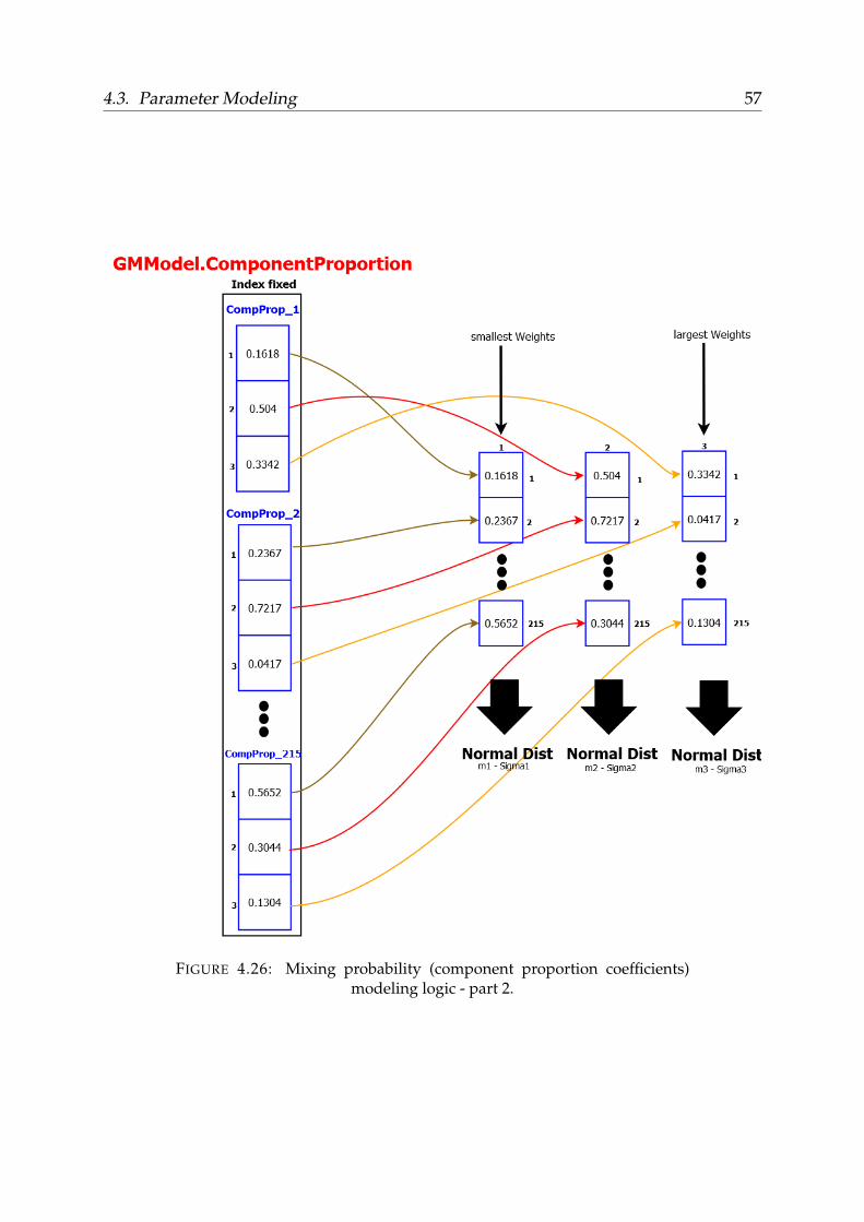
Each element is allocated in an array in the same manner as mean table parame-ter’s modeling. A Gaussian is fitted in each array thus creating a model of 3 normaldistributions describing the coefficients for Dt, meanF, len and 2 normal distributionsfor the angle. The aforementioned are depicted in Figure 4.26.
In summary, modeling component proportion coefficients of the GMMs starts atunification and index-fixing of the values. Then, a Gaussian is fitted for each compo-nent. Therefore, Dt, meanF and len are statistically described using 3 normal distribu-tions while 2 normal distributions are used for the angle resulting in a total of 5 normaldistributions.
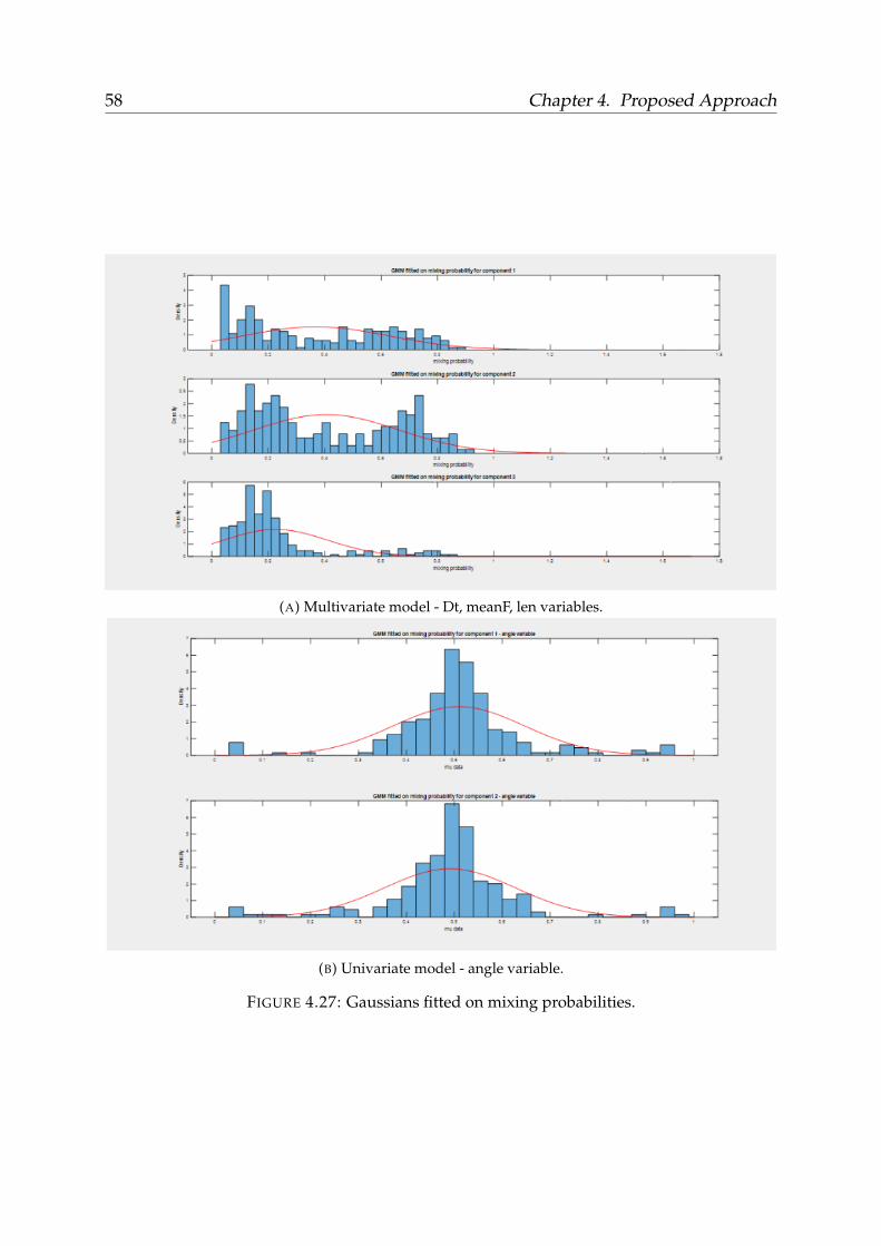
Figure 4.27 illustrates the Gaussians fitted on the mixing probabilities for the mul-tivariate and univariate model. We notice in the latter that the normal distributions aresimilar. This result is considered sensible as the probability of a step being performedon each direction is the same.
56 Chapter 4. Proposed Approach
FIGURE 4.25: Mixing probability (Component Proportion Coefficients)modeling logic - part 1.
4.3. Parameter Modeling 57
FIGURE 4.26: Mixing probability (component proportion coefficients)modeling logic - part 2.
58 Chapter 4. Proposed Approach
(A) Multivariate model - Dt, meanF, len variables.
(B) Univariate model - angle variable.
FIGURE 4.27: Gaussians fitted on mixing probabilities.
4.3.3 Statistical Description of the Variance/Covariance Matrix Σ
The variance/covariance matrix Σ parameter of a 3-variate GMM is a 3x3 symmetricand positive semi-definite matrix describing the covariance between variables as wellas the variances (matrix diagonal), i.e., the covariance of each random variable withitself.
Consequently, the critical values of a 3-variate covariance matrix are 6. Those arethe 3 diagonal values i.e., the variance of each variable, as well as the covariancesbetween the 1st and 2nd variable, the 1st and 3rd variable and finally, the 2nd and3rd variable. Thus, for the most accurate statistical description of Σ, a unified tablecontaining the 6 differentiated values of all subjects was created and a Gaussian isfitted in each, as illustrated in Figure 4.28.
60 Chapter 4. Proposed Approach
(A) Multivariate model - Dt, meanF, len variables.
(B) Univariate model - angle variable.
FIGURE 4.29: Gaussians fitted in variance/covariance matrix Σ.
In summary, modeling variance/covariance matrix Σ of the GMMs starts at unifi-cation of it’s critical values. Then, a Gaussian is fitted for each. Therefore, Dt, meanFand len are statistically described using 6 normal distributions while 1 more is usedfor the angle as a univariate GMM is described only by it’s variance. Thus, a total of 7normal distributions is required for the modeling of Σ. Figure 4.29 depicts the Gaus-sians fitted on the critical values of Σ for the multivariate and the univariate model,respectively.
4.4. Modeling Overview 61
4.4 Modeling Overview
The statistical description of the parameters of the Gaussian Mixture Models con-cludes the process of modeling the human walk. This modeling was, in summary,implemented following the steps described in the previous sections of chapter 4.
The first step was to extract the necessary variables to describe a human walk us-ing the data contained in the provided database. These variables where the interarrivaltime of each step (Dt), the mean vertical force induced in a step (meanF), the length tra-versed (len) and the angle of each step. Those variables were extracted for each step ofeach person. Then, 2 GMMs were fitted in each person’s walks; a 3-component multi-variate for Dt, meanF and len and a 2-component univariate for the angle variable.
Finally, the statistical description of the parameters of those GMMs was conducted.More specifically, each GMM is parameterized by its mixing probability (componentproportion coefficients), mean table (mu) and covariance matrix Σ. Hence, upon someprocedures, these parameters were fitted in GMMs in order to statistically describethem. The statistical description of the multivariate GMM’s parameters (describingDt, meanF, len) resulted in:
• 9 Gaussians to describe the mean table parameter – 3 for each variable as theGMM consists of 3 components.
• 3 Gaussians to describe the mixing probability (component proportion coeffi-cients) parameter as the GMM consists of 3 components.
• 6 Gaussians to describe the Σ parameter - each Sigma is a 3x3 symmetric matrixas the GMM describes 3 variables and thus, there are 6 critical values.
While the statistical description of the univariate GMM describing the angle variableresulted in:
• 2 Gaussians to describe the mean table parameter as the GMM consists of 2 com-ponents.
• 2 Gaussians to describe the mixing probability (component proportion coeffi-cients) parameter as the GMM consists of 2 components.
• 1 Gaussian to describe the Σ parameter as the GMM describes 1 variable.
The diagram of Figure 4.30 shows an overview of this procedure.
62 Chapter 4. Proposed Approach
FIGURE 4.30: An overview of modeling human walk.
4.5. The Simulator 63
4.5 The Simulator
The scope of the simulator is to describe a random human walk accurately by extract-ing n sets of the 4 variables for n desired finite number of steps. In order to achieve this,a reversed procedure than the one followed for the modeling will be conducted. Morespecifically, the goal is to extract a random walk using the statistical description of theparameters acquired through the modeling, as input. Thus, a random generation ofthe parameters is performed using the models describing them. Then, a multivariateand a univariate GMM is fitted using the respective parameters. These GMMs willbe used as distributions that best describe the process of human walk. Consequently,using these GMMs, n sets of the Dt, meanF, len and angle random variables will beacquired. Those sets will describe a random walk of n steps. This process is depictedgraphically in the diagram of Figure 4.35.
4.5.1 Parameter Estimation
The first step of our implementation is to generate a set of parameters to use on theGMM statistically describing the human walk. In the same manner, the multivariateGMM’s variables i.e., Dt, meanF, len will be extracted first.
Consequently, using the 3 Gaussians describing the mean values of each variablei.e., 9 Gaussians in total, a random value is generated using each one. Thus, the 3Gaussians produce 3 random values for each of the three random variables and theunification of those produces the final mean table which will be used as a parameter inthe simulated GMM (Figure 4.31).
Likewise, the mixing probability or component proportion coefficients parameterof the simulated GMM is generated using the 3 Gaussians created in the modeling.Thus, 3 values are generated and are used as parameters in the simulated GMM (Fig-ure 4.32). Note that the mixing probabilities must sum to 1. However, since these arerandomly generated, this constraint is not always satisfied and therefore, a normaliza-tion in the generated mixing probabilities is performed.
FIGURE 4.31: Generating a random mean table.
64 Chapter 4. Proposed Approach
FIGURE 4.32: Generating random mixing probability (component propor-tion coefficients).
FIGURE 4.33: Generating a random variance/covariance matrix Σ.
Finally, the variance/covariance matrix Σ of the simulated GMM is generated usingthe 6 Gaussians created in the modeling. More specifically, the 6 critical values arerandomly generated by these Gaussians. The first 3 values describe the diagonal valuesof the matrix i.e., variance of each variable, while the fourth describes the covariancebetween the first and second variable i.e., the values (1,2) and (2,1) of the Σ matrix.Finally, the fifth describes the covariance between the first and the third variable i.e.,values (1,3) and (3,1) of the Σ matrix and finally, the sixth describes the covariancebetween the second and the third variable i.e., values (2,3) and (3,2) of the Σ matrix.This way, a symmetrical covariance matrix is generated (Figure 4.33).
The only constraint in this procedure is that, as it is known by the theory, a co-variance matrix, apart from symmetrical, is also positive semi-definite. However, therandom generation does not guarantee this. To confront this, a workaround has beenimplemented and therefore, the random generation is performed in a loop that breakswhen the generated matrix is positive semi-definite.
The same procedure is performed for the extraction of the parameters characteriz-ing the simulated univariate GMM describing the random variable of angle. In thiscase, the mean table parameter is determined by randomly generating the 2 necessaryvalues using the 2 Gaussians describing it. The same applies to the extraction of themixing probability, whereas the 2 values are generated and normalised in order to sumto 1. Finally, the Gaussian describing the variance of the variable is used to randomlygenerate the value of σ. This procedure is depicted in Figure 4.34
4.5.2 Extraction of the Random Walk
In the final step, two GMMs i.e., a multivariate for Dt, meanF, len and a univariatefor the angle, are fitted using the random parameters generated in subsection 4.5.1as input. Using these GMMs, the random walk is extracted. The multivariate GMM
4.5. The Simulator 65
FIGURE 4.34: Generating random parameters for the angle variable.
generates n sets of Dt, meanF and len variables while the GMM describing the anglegenerates n values of the angle variable. The merging of those describes a randomwalk of n steps.
66 Chapter 4. Proposed Approach
FIGURE 4.35: An overview of the simulator.
67
Chapter 5
Experimental Setup
5.1 Instruments Used for the Analysis
The data used in this work have been acquired through an experimental campaign [17,39] conducted at the University of Modena and Reggio Emilia, Department of Engi-neering “Enzo Ferrari” (Modena, Italy) and were provided beforehand. More specifi-cally, an instrumented floor equipped with a sensor system has been exploited to mea-sure the force, time, and position of each step. The setup used to make the measure-ments consists of 10 plates that occupy an area of 1m2, each, placed sequentially in ahorizontal formation yielding an area of 2x5 for a total of 10m2 of available surface onthe walkway, as illustrated in Figure 5.1. These plates are constructed of stainless steeland covered with waterproof mats made of synthetic material steel.
It is worth pointing out that this approach allows to acquire the quantity of interestdirectly. Other available methods used in the literature indeed involve uncertainties.An example of this is if, the measurement of the acceleration was acquired using anaccelerometer constrained to a foot. In fact, the human body is not a rigid system andthe force applied to the floor cannot be simply inferred from the acceleration and thestatic mass of the person.
Force sensors are installed beneath each vertex of the plates (Figure 5.2) so that theinduced force can be measured. Additionally, the position of the applied force can beinferred through simple trigonometric manipulation. The output of the force sensors isacquired through an acquisition system that consists of a control unit and a computerand is manufactured by National Instrument.
It is important to note that the algorithms, diagrams and extracted results describedin chapter 4 and chapter 6 were implemented using MATLAB R2019b Update 7 [29].
68 Chapter 5. Experimental Setup
FIGURE 5.1: The instrumented floor used in the experiments. [17, 39]
FIGURE 5.2: Force sensors installed beneath the vertices of the plates. [17,39]
5.2. Critical Factors in the Analysis 69
5.2 Critical Factors in the Analysis
The data collected in this study are conditioned by several factors. More specifically,the data relating to the right and left plates were acquired separately. Therefore, thegait of each subject was "guided" towards the center line of the floor.
Secondly, it is important to note that the plates of the instrumented floor could pro-duce noise during the experiments due to the extreme sensitivity of the data. Actually,the software used for the data processing showed some small abnormal variations inthe force induced on certain plates.
Thirdly, the subjects tested differed in height and weight i.e. the speed varies oneach subject. As known from the literature, as speed varies, the shape of the stepchanges, hence, a metronome was used to obtain time histories of the step at a fixedrate.
Lastly, the experiments were designed for individuals walking at a normal tempoand thus, the presence of other pedestrians in the walkway, the resonance phenomenon,the contingency of a collision, a random roaming, jogging, running, etc. are not takeninto consideration, as a real-world example would require.
71
Chapter 6
Simulations & Evaluation
Similarly to Figure 4.11, Figure 6.1 depicts an instance of the table extracted by the sim-ulator describing a randomly generated human gait of 30 steps. The columns of thetable correspond to the variables of interarrival time (Dt), mean vertical force induced(meanF), length (len) and angle of each step, respectively.
As a first deduction by comparing the two tables, the values generated can be con-sidered comparable to the values of a random person from the database. The onlyremarkable difference spotted is in the meanF variable. Figure 4.11 is probably de-scribing a human with large weight whose walking induces a big force on each step.However, the database includes measurements for a variety of body types and sexesand as a result, the simulated values of force contain values with great modulation.
To deepen our understanding about the outcome of the simulator, the mean speedof gait was calculated in order to compare it with the theoretical mean speed of humanwalking at a normal tempo. Using the len and Dt variables, speed can be calculated as:
speed =length
Dt(6.1)
Equation 6.1 produces the speed of each step. The mean speed 1000 random walksimulations of n = 30 steps, was calculated as:
mean speed = 5.2 km/h
The average speed of human walk at a normal tempo is ranging from 4.51 km/hto 4.75 km/h for older individuals and from 5.32 km/h to 5.43 km/h for youngerindividuals [56, 3]. Thus the simulated walk’s speed approximates the expected value.
Finally, using the length and the angle of each step acquired by the simulated walk,the x and y positions of each step j were calculated as:
xj =
{xj−1 + len cos (angle), if j > 1len cos (angle), if j = 1
}and yj = len sin (angle) (6.2)
These positions were scattered in Figure 6.2 in order to visualise the simulated humanwalk on the walkway.
Finally, Figure 6.3 depicts the first (out of two) walk of the subject of Figure 4.11.Note that the randomly generated walk approximates the pattern of the experimental.
72 Chapter 6. Simulations & Evaluation
FIGURE 6.1: A random walk generated for n = 30 steps.
Chapter 6. Simulations & Evaluation 73
FIGURE 6.2: Scattering a random walk.
FIGURE 6.3: First walk of the random subject described in Figure 4.11.
74 Chapter 6. Simulations & Evaluation
In conclusion, it can be inferred that the outcome of the simulator is promising asthe data generated match the properties of the experimental quite efficiently. Thus, thissimulator is capable of supplementing the experimental procedure in future research.
75
Chapter 7
Conclusion & Future Work
7.1 Conclusion
In this thesis, we presented an innovative algorithm for modeling and simulation ofhuman gait using Gaussian Mixture Models and Normal Distributions. More specifi-cally, we presented a practical model to use at the design stage of a walkway that sat-isfies the requirements of simplicity i.e., the GMMs and Gaussians used require simplecalculations, ease of use by engineers as well as accuracy i.e., a large number of ex-perimental samples is used. Furthermore, this algorithm can be considered innovativei.e., we used GMMs and conceived the human walk as a random process, while only afew past researches with a small number of data have done so. Lastly, in the proposedmodel we accounted the intersubject and intrasubject variability model.
We also implemented a simulator that can be used to provide reliable predictionand assessment of floor vibrations under human actions, using the developed mod-els. Thus, using this approach, the experimental procedure can be omitted in futureresearches.
7.2 Future Work
We conclude this thesis by presenting possible future extensions of this work. The nextstep to our research is to apply the simulator at a digital pedestrian walkway in orderto conduct research on bridge oscillations and the resonance effect using simulatedwalks. This digital pedestrian walkway is developed by the Civil and EnvironmentalEngineering Department of the University of Modena & Reggio Emilia (Dipartimentodi Ingegneria "Enzo Ferrari”).
Moreover, it would be practical to repeat the experimental campaign using a big-ger instrumented floor that approximates the dimensions of a real footbridge, thusallowing for more steps at each stride. In this case, the experimental procedure wouldpreferably include more information about the characteristics of the subjects e.g., gen-der, physical characteristics, nation, culture, the environment, etc. These parametersinfluence the intersubject variability of human walking process as suggested by sev-eral researches [23, 62, 66] presented in section 3.3.
Using these information, the model can be extended to include real world occasionse.g., the presence of many pedestrians in the walkway, the synchronization of step
76 Chapter 7. Conclusion & Future Work
within groups, the contingency of a collision, a random roaming, jogging, running,etc.
77
Bibliography
[1] TP Andriacchi, JA Ogle, and JO Galante. “Walking speed as a basis for normaland abnormal gait measurements”. In: Journal of biomechanics 10.4 (1977), pp. 261–268.
[2] Andreas Antoniou. Digital filters: analysis, design, and signal processing applications.2018.
[3] Karen Aspelin and Nick Carey. “Establishing pedestrian walking speeds”. In:Portland State University (2005), pp. 5–25.
[4] Ed Ayyappa. “Normal human locomotion, part 1: Basic concepts and terminol-ogy”. In: JPO: Journal of Prosthetics and Orthotics 9.1 (1997), pp. 10–17.
[5] Hugo Bachmann and Walter Ammann. Vibrations in structures: induced by manand machines. Vol. 3. Iabse, 1987.
[6] Hugo Bachmann et al. Vibration problems in structures: practical guidelines. Birkhäuser,2012.
[7] J Blanchard, BL Davies, and JW Smith. “Design criteria and analysis for dynamicloading of footbridges”. In: Proceeding of a Symposium on Dynamic Behaviour ofBridges at the Transport and Road Research Laboratory, Crowthorne, Berkshire, Eng-land, May 19, 1977. TRRL Rpt. 275 Proceeding. 1977.
[8] J MW Brownjohn, Aleksandar Pavic, and P Omenzetter. “A spectral density ap-proach for modelling continuous vertical forces on pedestrian structures due towalking”. In: Canadian Journal of Civil Engineering 31.1 (2004), pp. 65–77.
[9] J. M. W. Brownjohn and A. Pavic. “Human-Induced Vibrations on Footbridges”.In: Advances in Bridge Maintenance, Safety Management, and Life-Cycle Performance:Proceedings of the Third International Conference on Bridge Maintenance, Safety andManagement (IABMAS), Porto, Portugal (2015), pp. 263–264.
[10] James Brownjohn, Vitomir Racic, and Jun Chen. “Universal response spectrumprocedure for predicting walking-induced floor vibration”. In: Mechanical Sys-tems and Signal Processing 70 (2016), pp. 741–755.
[11] Thomas Caleri. “Sviluppo di un modello matematico per la camminata bipede:Fitting e studio di una distribuzione multivariata che ne approssimi l’andamento”.In: Università degli Studi di Modena e Reggio Emilia, 2018.
[12] Anil K Chopra. “Dynamics of Structures Prentice-Hall”. In: Englewood Cliffs, NJzbMATH (1995).
78 Bibliography
[13] Brad Davis and Onur Avci. “Simplified vibration serviceability evaluation ofslender monumental stairs”. In: Journal of Structural Engineering 141.11 (2015),p. 04015017.
[14] Brad Davis, Di Liu, and Thomas M Murray. “Simplified experimental evalua-tion of floors subject to walking-induced vibration”. In: Journal of Performance ofConstructed Facilities 28.5 (2014), p. 04014023.
[15] A Ebrahimpour et al. “Measuring and modeling dynamic loads imposed bymoving crowds”. In: Journal of Structural Engineering 122.12 (1996), pp. 1468–1474.
[16] Per-Erik Eriksson. Vibration of low-frequency floors-dynamic forces and response pre-diction. Chalmers University of Technology, 1994.
[17] Martina Fornaciari. “Sviluppo di un modello matematico per la camminata bi-pede: applicazione nello studio di stabilità delle passerelle ciclopedonali”. In:Università degli Studi di Modena e Reggio Emilia, 2018.
[18] FW Galbraith and MV Barton. “Ground loading from footsteps”. In: The Journalof the Acoustical Society of America 48.5B (1970), pp. 1288–1292.
[19] F. C. Harper. “The Mechanics of Walking”. In: Res. Appl. Ind 15.1 (1962), pp. 23–28.
[20] Jeffrey M Hausdorff. “Gait dynamics, fractals and falls: finding meaning in thestride-to-stride fluctuations of human walking”. In: Human movement science 26.4(2007), pp. 555–589.
[21] EJ Hudson et al. “Active Control of Concert-Induced Vibrations”. In: Geotechnicaland Structural Engineering Congress 2016. 2016, pp. 1729–1741.
[22] VT Inman, HJ Ralston, and F Todd. “Human walking-Williams and Wilkins”. In:Baltimore, London (1981).
[23] Tianjian Ji and Aikaterini Pachi. “Frequency and velocity of people walking”. In:Structural Engineer 84.3 (2005), pp. 36–40.
[24] CA Jones, P Reynolds, and A Pavic. “Vibration serviceability of stadia structuressubjected to dynamic crowd loads: A literature review”. In: Journal of Sound andVibration 330.8 (2011), pp. 1531–1566.
[25] M Kasperski and C Sahnaci. “Serviceability of pedestrian structures”. In: Pro-ceedings of the International Modal Analysis Conference (IMAC XXC), Orlando, USA.2007.
[26] Stuart Clifford Kerr. “Human induced loading on staircases”. PhD thesis. Uni-versity of London, 1998.
[27] H Kramer and HW Kebe. “Man-induced structural vibrations”. In: Der Bauinge-nieur 54.5 (1980), pp. 195–199.
[28] Di Liu and Brad Davis. “Walking vibration response of high-frequency floorssupporting sensitive equipment”. In: Journal of Structural Engineering 141.8 (2015),p. 04014199.
Bibliography 79
[29] MATLAB. 9.7.0.1190202 (R2019b). Natick, Massachusetts: The MathWorks Inc.,2018.
[30] Y Matsumoto et al. “A study on design of pedestrian over-bridges”. In: Transac-tions of JSCE 4 (1972), pp. 50–51.
[31] Jack C McCormac and Stephen F Csernak. Structural steel design. pearson prenticehall Upper Saddle River, 2008.
[32] Neil Messenger. “Moving the human machine: understanding the mechanicalcharacteristics of normal human walking”. In: Physics Education 29.6 (1994), pp. 352–357.
[33] CJ Middleton and JMW Brownjohn. “Response of high frequency floors: A liter-ature review”. In: Engineering Structures 32.2 (2010), pp. 337–352.
[34] TM Murray, DE Allen, and EE Ungar. “Design guide 11, floor vibrations due tohuman activities”. In: American Institute of Steel Construction (AISC), Chicago, IL(2003).
[35] Karl M Newell and Andrew B Slifkin. “The Nature of Movement”. In: Motorbehavior and human skill: A multidisciplinary approach (1998), p. 143.
[36] Antonio Occhiuzzi, Mariacristina Spizzuoco, and Francesco Ricciardelli. “Load-ing models and response control of footbridges excited by running pedestrians”.In: Structural Control and Health Monitoring: The Official Journal of the InternationalAssociation for Structural Control and Monitoring and of the European Association forthe Control of Structures 15.3 (2008), pp. 349–368.
[37] Antonio Occhiuzzi, Mariacristina Spizzuoco, and Francesco Ricciardelli. “Load-ing models and response control of footbridges excited by running pedestrians”.In: Structural Control and Health Monitoring: The Official Journal of the InternationalAssociation for Structural Control and Monitoring and of the European Association forthe Control of Structures 15.3 (2008), pp. 349–368.
[38] Sven V Ohlsson. Floor vibrations and human discomfort. Chalmers University ofTechnology, Division of Steel and Timber Structures, 1982.
[39] Milani Pancaldi Bassoli and Vincenzi. “A Statistical Approach for Modelling In-dividual Walking Forces”. In: Elsevier MSSP, 2020.
[40] A Pavic et al. “Critical review of guidelines for checking vibration serviceabilityof post-tensioned concrete floors”. In: Cement and Concrete Composites 23.1 (2001),pp. 21–31.
[41] Aleksandar Pavic and Paul Reynolds. “Vibration serviceability of long-span con-crete building floors. Part 1: Review of background information”. In: Shock andVibration Digest 34.3 (2002), pp. 191–211.
[42] Aleksandar Pavic and Paul Reynolds. “Vibration serviceability of long-span con-crete building floors. Part 2: Review of mathematical modelling approaches”. In:Shock and Vibration Digest 34.4 (2002), pp. 279–297.
80 Bibliography
[43] Aleksander Pavic and MR Willford. “Appendix G: Vibration serviceability ofpost-tensioned concrete floors”. In: Post-tensioned concrete floors design handbook(2005), pp. 99–107.
[44] Matjaž Perc. “The dynamics of human gait”. In: European journal of physics 26.3(2005), p. 525.
[45] Vitomir Racic, James Brownjohn, and Aleksandar Pavic. “Dynamic loading fac-tors of individual jogging forces”. In: ECCOMAS proceedings. 2013.
[46] Vitomir Racic and James Mark William Brownjohn. “Stochastic model of near-periodic vertical loads due to humans walking”. In: Advanced Engineering Infor-matics 25.2 (2011), pp. 259–275.
[47] Vitomir Racic, James MW Brownjohn, and Aleksandar Pavic. “Random modelof vertical walking force signals”. In: Topics on the Dynamics of Civil Structures,Volume 1. Springer, 2012, pp. 73–84.
[48] Vitomir Racic and JMW Brownjohn. “Mathematical modelling of random nar-row band lateral excitation of footbridges due to pedestrians walking”. In: Com-puters & structures 90 (2012), pp. 116–130.
[49] Vitomir Racic and A Pavic. “Mathematical model to generate near-periodic hu-man jumping force signals”. In: Mechanical Systems and Signal Processing 24.1(2010), pp. 138–152.
[50] Vitomir Racic, Aleksandar Pavic, and JMW Brownjohn. “Experimental identifi-cation and analytical modelling of human walking forces: Literature review”. In:Journal of Sound and Vibration 326.1-2 (2009), pp. 1–49.
[51] JH Rainer, G Pernica, and David E Allen. “Dynamic loading and response offootbridges”. In: Canadian Journal of Civil Engineering 15.1 (1988), pp. 66–71.
[52] C Sahnaci and M Kasperski. “Random loads induced by walking”. In: Proceedingsof the sixth European conference on structural dynamics. Vol. 1. 2005, pp. 441–6.
[53] J. Simpson and E. Weiner. The Oxford English Dictionary. Oxford University Press,1989. ISBN: 9780191958922.
[54] Andrew L Smith, Stephen J Hicks, and Paul J Devine. Design of floors for vibration:A new approach. Steel Construction Institute Ascot, Berkshire, UK, 2007.
[55] Steven W Smith et al. “The scientist and engineer’s guide to digital signal pro-cessing”. In: (1997).
[57] Christopher L Vaughan, Brian L Davis, Jeremy C O’connor, et al. Dynamics ofhuman gait. Human Kinetics Publishers, 1992.
[58] John E Wheeler. “Prediction and control of pedestrian-induced vibration in foot-bridges”. In: Journal of the structural division 108.9 (1982), pp. 2045–2065.
[59] Michael W Whittle. Gait analysis: an introduction. Butterworth-Heinemann, 2014.
Bibliography 81
[60] M Willford, P Young, and C Field. “Predicting footfall-induced vibration: Part1”. In: Proceedings of the Institution of Civil Engineers-Structures and Buildings 160.2(2007), pp. 65–72.
[61] Michael R Willford, Peter Young, and MIMechE CEng. A design guide for footfallinduced vibration of structures. Concrete Society for The Concrete Centre, 2006.
[62] Richard Wiseman. Quirkology: the curious science of everyday lives. Pan Macmillan,2008.
[63] Wei-ping Xie, Liang Chang, and Yong Du. “Analysis on vibration isolation ofZhongnan Theater”. In: CHINESE JOURNAL OF GEOTECHNICAL ENGINEERING-CHINESE EDITION- 29.11 (2007), p. 1720.
[64] Masahiro Yoneda. “A simplified method to evaluate pedestrian-induced maxi-mum response of cable-supported pedestrian bridges”. In: Proceedings of the In-ternational Conference on the Design and Dynamic Behaviour of footbridges. 2002.
[65] P Young. “Improved floor vibration prediction methodologies. Engineering forStructural Vibration–Current developments in research and practice Arup Vibra-tion Seminar”. In: Institution of Mechanical Engineers (2001).
[66] Stana Zivanovic. “Probability-based estimation of vibration for pedestrian struc-tures due to walking.” PhD thesis. University of Sheffield, 2006.
[67] S Živanovic, A Pavic, and Vitomir Racic. “Towards modelling in-service pedes-trian loading of floor structures”. In: Topics on the Dynamics of Civil Structures,Volume 1. Springer, 2012, pp. 85–94.
[68] Stana Z˘ivanovic and Aleksandar Pavia. “Probabilistic assessment of human re-sponse to footbridge vibration”. In: Journal of low frequency noise, vibration andactive control 28.4 (2009), pp. 255–268.
[69] Stana Živanovic and A Pavic. “Probabilistic approach to subjective assessment offootbridge vibration”. In: The 42rd UK Conference on Human Responses to Vibration.2007.
[70] Stana Živanovic, ALEKSANDAR Pavic, and Paul Reynolds. “Vibration service-ability of footbridges under human-induced excitation: a literature review”. In:Journal of sound and vibration 279.1-2 (2005), pp. 1–74.
[71] Stana Živanovic and Aleksandar Pavic. “Probabilistic modeling of walking ex-citation for building floors”. In: Journal of performance of constructed facilities 23.3(2009), pp. 132–143.
[72] Stana Živanovic, Aleksandar Pavic, and Paul Reynolds. “Probability-based pre-diction of multi-mode vibration response to walking excitation”. In: Engineeringstructures 29.6 (2007), pp. 942–954.