SBi 2013:14

Study of a Two-Pipe Chilled Beam System for both Cooling and Heating of Office Buildings

Study of a Two-Pipe Chilled Beam System for both Cooling and Heating of Office Buildings Rouzbeh Norouzi, Göran Hultmark Alireza Afshari Niels Christian Bergsøe

SBi 2013:14 Danish Building Research Institute, Aalborg University · 2013

Title Study of a Two-Pipe Chilled Beam System for both Cooling and Heating of Office Buildings Serial title SBI 2013:14 Edition 1 edition Year 2013 Authors Rouzbeh Norouzi University of Borås, Göran Hultmark Lindab Comfort A/S, Alireza Afshari

Statens Byggeforskningsinstitut ved Aalborg Universitet, Niels Christian Bergsøe Statens Byggeforskningsinstitut ved Aalborg Universitet

Editor Alireza Afshari Language English Pages 45 References Page 42 Key words Chilled Beam System, Cooling, Heating, Office Buildings ISBN 978-87-92739-36-0 Drawings Rouzbeh Norouzi and Lindab Comfort A/S Publisher SBi, Statens Byggeforskningsinstitut, Aalborg Universitet,

Danish Building Research Institute, Aalborg University A.C. Meyers Vænge 15, DK-2450 Copenhagen SV E-mail sbi@sbi.aau.dk www.sbi.dk

This publication is covered by the Danish Copyright Act

Content

Preface ............................................................................................................ 4 Executive Summary ........................................................................................ 5 Introduction ...................................................................................................... 6

Background ................................................................................................. 6 Active Chilled Beams system for comfort according to ASHRAE .............. 7 Requirements to an active chilled beam ..................................................... 8

Objectives and scope .................................................................................... 12 Methodology and the key topics in this work ................................................. 13

Two-Pipe System and CACB introduction ................................................ 13 Simulation tool .......................................................................................... 15 Building model .......................................................................................... 15 HVAC System Model ................................................................................ 18 Calculation methods ................................................................................. 24

Result ............................................................................................................ 31 Discussion ..................................................................................................... 37 Conclusion ..................................................................................................... 41 References .................................................................................................... 42 Appendix 1 ..................................................................................................... 44

Maximum heating demand in the year ..................................................... 44 Mollier diagram for ventilation calculation ................................................. 45

3

Preface

A chilled beam system can be used for ventilation, cooling and heating of of-fice buildings for thermal comfort. In this project, the possibility of using the same pipes for both heating and cooling was investigated, depending on the requirements pertaining to the heating and cooling seasons. The main objec-tive of this project is to study requirements, possibilities and limitations for a well-functioning 2-pipe system for both cooling and heating of office build-ings. This project was introduced by the Danish Building Research Institute / Aalborg University (SBI/AAU) in collaboration with Lindab Comfort A/S. Many people have helped with the work during my thesis work in the form of shared knowledge and experiences and supporting. Thanks to: Senior Re-searcher Kim Bjarne Wittchen and Senior Researcher Kjeld Johnsen from SBi/AAU, Magnus Jacobsson, Anders Vorre, Daniel Bochen, Dohnal Miro-slav and Nicolai Skovsager Bang from Lindab. Danish Building Research Institute, Aalborg University Department of Energy and Environment May 2013 Søren Aggerholm Head of the department

4

Executive Summary

The main aim of this master thesis was to investigate possibilities and limita-tions of a new system in active chilled beam application for office buildings. Lindab Comfort A/S pioneered the presented system. The new system use two-pipe system, instead of the conventional active chilled beam four-pipe system for heating and cooling purposes. The Two-Pipe System which is studied in this project use high temperature cooling and low temperature heating with water temperatures of 20°C to 23°C, available for free most of the year. The system can thus take advantage of renewable energy. It was anticipated that a Two-Pipe System application enables transfer of energy from warm spaces to cold spaces while return flows, from cooling and heat-ing beams, are mixed. BSim software was chosen as a simulation tool to model a fictional office building and calculate heating and cooling loads of the building. Moreover, the effect of using outdoor air as a cooling energy source (free cooling) is investigated through five possible scenarios in both the four pipe system and the Two-Pipe System. The calculations served two purposes. Firstly, the effect of energy transfer in the Two-Pipe System were calculated and compared with the four pipe system. Secondly, free cooling effect was calculated in the Two-Pipe System and compared with the four pipe system. The simulation results showed that the energy transfer, as an inherent characteristic in the Two-Pipe System, is able to reduce up to 3 % of annual energy use compared to the four pipe system. Furthermore, different free cooling applications in the Two-Pipe System and the four pipe system re-spectively showed that the Two-Pipe System requires 7-15 % less total en-ergy than the four pipe system in one year. In addition, the Two-Pipe System can save 18-57 % of annual cooling energy when compared to the four pipe system.

5

Introduction

Background

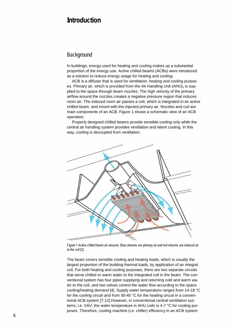
In buildings, energy used for heating and cooling makes up a substantial proportion of the energy use. Active chilled beams (ACBs) were introduced as a solution to reduce energy usage for heating and cooling. ACB is a diffuser that is used for ventilation, heating and cooling purpos-es. Primary air, which is provided from the Air Handling Unit (AHU), is sup-plied to the space through beam nozzles. The high velocity of the primary airflow around the nozzles creates a negative pressure region that induces room air. The induced room air passes a coil, which is integrated in an active chilled beam, and mixed with the injected primary air. Nozzles and coil are main components of an ACB. Figure 1 shows a schematic view of an ACB operation. Properly designed chilled beams provide sensible cooling only while the central air handling system provides ventilation and latent cooling. In this way, cooling is decoupled from ventilation.

Figure 1 Active chilled beam air streams: Blue streams are primary air and red streams are induced air to the coil [2].

The beam covers sensible cooling and heating loads, which is usually the largest proportion of the building thermal loads, by application of an integral coil. For both heating and cooling purposes, there are two separate circuits that serve chilled or warm water to the integrated coil in the beam. The con-ventional system has four pipes supplying and returning cold and warm wa-ter to the coil, and two valves control the water flow according to the space cooling/heating demand [4]. Supply water temperature ranges from 14-18 °C for the cooling circuit and from 30-45 °C for the heating circuit in a conven-tional ACB system [7,12].However, in conventional central ventilation sys-tems, i.e. VAV, the water temperature in AHU coils is 4-7 °C for cooling pur-poses. Therefore, cooling machine (i.e. chiller) efficiency in an ACB system

6

(independent of ventilation system) is 15-20 % higher than in conventional central air systems [8]. The major limitation is the application of the ACBs in spaces where the la-tent load is significant. High latent load means high moisture load and it con-sequently leads to condensation on the exposed surfaces of the cooling coil. Hence, the beams are suitable for application in offices and commercial buildings where the moisture production is low. Otherwise, the active chilled beam system should be equipped with a humidity control system. In four-pipe hydronic systems, i.e. Conventional ACB system, the heating system and cooling system operate individually. It is very common that the system provides cooling for one space and heating for another space at the same time. Heating and cooling overlap causes 5-20 % waste of energy when the two systems are operating to neutralise each other [9]. Reduction of the heating and cooling overlap is a consideration in the design process of four-pipe hydronic systems. This study investigates possibilities and limitations using a Two-Pipe Sys-tem for both heating and cooling in ACB application instead of a four-pipe system. The Two-Pipe system is based on supplying higher temperature wa-ter for cooling and lower temperature water for heating than the conventional active chilled beams.

Active Chilled Beams system for comfort according to ASHRAE

Active chilled beams (ACBs) are not only in-room heating and cooling devic-es, but also a diffusor that supplies conditioned air to the rooms. Thus, ACBs are supposed to provide an acceptable level of thermal comfort for the occu-pants in order to meet the requirements of ASHRAE 55 [3]. The ASHRAE standard defines an occupied zone as a part of the total room volume where the occupant resides. The occupied zone is specified as not closer than 1 m from the outside wall or window and not closer than 0.3 m from internal walls. The standard defines the occupied zone height is 1.1 m for a seated occupant [3]. The criteria for thermal comfort, according to ASHRAE 55, define the maximum of 3 °C of the vertical thermal gradient as the limit for thermal comfort [3]. It means that maximum bottom-to-top temperature difference in the occupied zone should not exceed 3 °C. On the other hand, although a reduction of the primary airflow is an ad-vantage of ACBs, the reduction should be limited to meet humidity level re-quirements and to supply required fresh air to the spaces. The humidity level should be controlled in order to prevent condensation on surfaces and to provide a comfortable indoor climate for occupants. Condensation occurs when the water temperature in the beam is below room air dew point tem-perature. On the other hand, fresh air minimum requirement should be pro-vided by ventilation air. Hence, adequate primary airflow is needed to ex-haust humid air from rooms and supply fresh air with suitable humidity level to rooms. Furthermore, active chilled beams should be designed to have an appro-priate air velocity to prevent draught and consequently to avoid disturbance for occupants of the occupied zone. The standard defines maximum air ve-locity, in occupied zone, as 0.25 m/s [3]. The application of active chilled beams should meet the requirements for humidity level, fresh air supply, air-supply velocity and space thermal com-fort.

7

Requirements to an active chilled beam

Construction requirements An ACB is installed as an integrated unit with an acoustical ceiling and it re-quires less ceiling space than traditional HVAC systems (e.g. VAV) [3, 11]. As mentioned in section “Two-Pipe System and CACB introduction”, page 13 the ACB system requires smaller duct system since it requires less air-flow than all-air systems. For example, an office room with a floor area of 10 m2 requires 14 l/s primary air in an active chilled beam system while the room requires 47 l/s ventilation air in VAV system [11]. Hence, less ducting system size in the ACB system results in less floor-to-floor height require-ment. Less floor-to-floor height leads to reduction in construction cost of the ACB system than all-air systems like VAV system.

Installation requirements An ACB system installation has some considerations that are similar to fan coil system installation. For instance, ACBs require hangers, sensors and piping systems like fan coil system. Thus, the installation procedure is similar to fan coils installation. However, an ACB installation does not require elec-trical power supply like fan coils since there is no electrical motor in the ACB [4].

Operational requirements ACBs operation should meet some requirements to be able to provide indoor comfort climate. First, condensation protection is needed when an ACB is used for spaces with high latent load. Humidity control strategy (i.e. a humidity sensor on ex-hausted air flow) should be considered in Active chilled beam application to avoid surface condensation. Second, the ACBs application has limitations for cooling and heating ca-pacities. ACB applications are more recommended for spaces where the cooling demand and the heating demand are not more than 120 W/m2 and 40 W/m2 respectively in order to provide convenient indoor climate for the occupants [12]. Third, the velocity of airflow and room temperature should meet criteria (e.g. ASHRAE 55) in order to avoid risk of draught in the occupied zone. In this study, a new active chilled beam application (Two-Pipe System) is investigated for energy potential. Maintenance, construction and installation requirements for the new concept are not considered. It is expected that the installation costs for the piping system in a Two-Pipe System are less than in a conventional four-pipe system.

8

Technical and design criteria of an Active Chilled Beam

Air supply The airflow rate plays a crucial role in the ACB design procedure. The beam operates only as an expensive diffuser when the air supply through nozzles covers most of the space cooling (or heating) load and the regulating valves in water circuits remain closed in the coil part of the beam [6]. Oversizing of the primary airflow system results in less efficiency in the water part of the ACB system and, consequently, the coil part of the beam does not operate at full capacity. The primary airflow, which is conditioned in the AHU, is supplied through the ACB nozzles and it is mixed with induced room air passed over the beam coil. The typical primary airflow rate for office buildings is recommend-ed in standards (e.g. REHVA) within the range of 1.5-3 l/s per m2 [12]. The flow rate range satisfies the fresh air requirements, acceptable humidity lev-el, air induction and comfort conditions [12]. In different seasons the primary air temperature range is different. Recommended primary air temperatures in summer and winter are 18-20 °C and 19-21 °C, respectively [12]. Ventilation air in ACB systems requires outdoor air without any recircula-tion [4]. Consequently, there is a potential for decreasing the ventilation air-flow rate to minimum fresh air requirements for the spaces. Although, the air flow rate should be sufficient to remove humidity and to induce room air to pass over the coil part of the beam, ventilation air reduction in the ACB sys-tem results in smaller duct size than all-air systems in which all loads should be covered by ventilation air. In this project, the new Two-Pipe System focuses on the water-system aspect in the ACBs. The functionality of the ventilation system is expected to be same (CAV system with a flow rate of 2.5 l/s per m2) as a conventional active chilled beams system.

Water supply A conventional four-pipe active chilled beam (CACB) has two water circuits to supply and return water to and from the beam coil. For cooling purposes, the water supply temperature in the CACBs is limited to minimum 14 °C, which is usually higher than the dew point temperature of room air to avoid condensation on coil surface [12]. On the other hand there is a limitation for heating application of the CACB. A warm water temperature higher than 45 °C in the circuit results in less air mixing between induced air and primary air and, therefore, it reduces beam efficiency and raises the vertical temperature gradient in the room. Typical water temperatures for heating purposes are 30-45 °C and for cool-ing 14-18 °C for the CACB system [12]. In a CACB system the water flow rate ranges between 0.025 and 0.1 kg/s. This range is selected to obtain turbulent flow in a 15 mm diameter pipe [12]. A turbulent water flow can transfer heat more efficiently than a laminar flow [12]. In the Two-Pipe System the water temperature is supposed to be 20-23 °C for both cooling and heating purposes simultaneously. Lindab Comfort A/S has performed a series of laboratory tests with measurements of the room temperature and the effect of inlet water temperature [22]. It can be concluded from the tests that a beam with a cooling capacity of 547 W and with a temperature difference between inlet and outlet water of 3.2 °C the room temperature will be kept 3.48 °C higher than the water mean tempera-ture. In the Two-Pipe System it was assumed that the system carries water of 20 °C for cooling purposes. If the return flow temperature is 23.2 °C, the beam capacity will be 547 W with the same water-flow rate. Therefore, the room temperature in the system will be 3.48 °C higher than the water mean temperature ((20+23.2)/2=21.6 °C) which is 25 °C (=21.6+3.48). The room temperature ranges from 13-26 °C in cooling [12]. Therefore, the water tem-

9

perature in the Two-Pipe System (20-23 °C) meets the requirements for condensation avoidance and heating limitations mentioned above. Moreo-ver, the water flow rate is supposed to be in the same range as the CACB system. In order to make the issue more clear, the below calculation is used: The cooling power of the beam is calculated through: �̇� = �̇�𝑐 (𝑇𝑜𝑢𝑡 − 𝑇𝑖𝑛) (1) Where m is water mass flow rate (kg/s) c is water specific heat capacity (kJ/kg, °C ) Tout is water outlet temperature (°C) Tin is water inlet temperature (°C) According to test results: 547[W] = 0.041 [kg/s]∙4.18 [kJ/kg, °C ] (20.74-17.55) [°C] Hence, according to the test result the room temperature will be 22.6 °C, that is 3.48 °C higher than the mean water temperature (19.14 °C). If the system is supplied with 20 °C water, the above equation will be: 547=0.041*4.18*(23.2-20) Therefore, the water-flow rate does not need to be changed and the beam has the same capacity. However, the room temperature will be kept 3.48 °C higher than the mean water temperature (21.6 °C) and it will be around 25 °C.

Humidity control In order to control humidity in the spaces AHU dehumidifies outdoor air and supplies dry air to spaces as primary air. Meanwhile, water supply tempera-ture is limited to minimum 14 °C which is usually above the room-air dew point temperature to avoid condensation on coil surfaces [12]. The room air dew point depends on the humidity ratio and it increases as humidity in-creases. Hence, the temperature limitation of 14 °C can be changed either by effects of external humidity infiltration or internal moisture production. Therefore, ACB is applicable in spaces with high infiltration rate and high tolerance in humidity level if different water supply temperatures (above room-air dew point) are set. In addition, moisture production in the spaces should be considered to control the humidity level. In office buildings the moisture production is about 0.6 g water/kg air which is mostly due to human activities [20]. Therefore, air supply humidity level and the production of moisture (in the space) should be considered for defining water supply temperature in ACB application to be operated above room-air dew point.

Free cooling Free cooling is an opportunity to reduce cooling cost since it provides chilled water through the use of cold outdoor air without a cooling machine (e.g. chiller). Free cooling can be obtained in several ways. Air-cooled heat ex-changer, cooling tower, geothermal, deep-water resources (e.g. lakes) and night-cooled storage are resources for providing free cooling energy [3]. In order to take advantage of free cooling there should be a certain tem-perature gradient between the cooling agent (water) and the outdoor air temperature to be able to exchange heat. Obviously, the required tempera-ture gradient depends on the efficiency of the equipment that provides free chilled water.

10

In conventional active chilled beam (CACB) the water inlet temperature is 14-18 °C for cooling. However, in the Two-Pipe System the water inlet tem-perature is supposed to be 20-23 °C for both heating and cooling purposes. Since the Two-Pipe System is supplied with higher water temperature for cooling, free cooling can be utilised. In this project free cooling effects are investigated for the Two-Pipe System and the CACB system, respectively.

11

Objectives and scope

The main goal of this study is to investigate the energy-saving potential of a Two-Pipe active chilled beam system for office buildings. The system is ap-plicable for heating and cooling purposes. The project has been initiated by Lindab Comfort AS and there are two areas of interest:

- possibilities for transferring energy between spaces when there are simultaneous heating and cooling demand using a Two-Pipe System

- possibilities for using free cooling in combination with a Two-Pipe System or a conventional four-pipe active chilled beam system.

In this study, simulations are carried out for a fictional multi-storey office-building. The output data from BSim software is used in order to calculate the heat transfer potential in the Two-Pipe System. Free cooling energy for the CACB (four-pipe system) and the Two-Pipe System is investigated through five scenarios. Finally, the results of each concept are compared.

12

Methodology and the key topics in this work

In order to calculate the energy demand of an office building, a building model was created for simulation. The simulation was performed using BSim software, which gave an hourly load calculation. The cooling and heating systems are simulated as an active chilled beam system. Having calculated the hourly thermal load of the fictional building, the energy usage in conven-tional active chilled beam (CACB) system was compared with the new Two-Pipe System. In addition, this project aimed at analysing energy usage in the Two-Pipe System by implementing different scenarios of free cooling and hence an overview of energy saving possibilities in comparison with a conventional ac-tive chilled beam system (CACB).

Two-Pipe System and CACB introduction

In a Two-Pipe System there is just one water circuit used for supplying water for both heating and cooling and the water temperature is 20-23 °C. In a conventional four-pipe system (CACB) there are two water circuits that sup-ply warm water and cold water with temperature ranges of 14-18 °C and 30-45 °C respectively [12]. Figure 2 - 4 demonstrates the Two-Pipe System operation schematically. The figures indicate simultaneous cooling and heating, only heating and only cooling conditions respectively. Figure 2 illustrates a schematic view of the Two-Pipe System for a specif-ic time when there are equal cooling demand and heating demand in differ-ent thermal zones simultaneously. In the Two-Pipe System water tempera-ture increases in cooling ACB units while it absorbs heat from the spaces. On the other side of the building water temperature in heating ACB units de-creases when it releases heat to the heating demand spaces. When return water from cooling ACB units is mixed with return water from heating ACB units, the end-circuit return water temperature is equal to the water supply temperature. No temperature difference between supply and return water results in zero handling machine (either cooling machine or heating machine) operation, and the return flow circulates again as supply water flow. Therefore, it can be concluded that the energy is transferred be-tween thermal zones while the return flows are mixed. Figure 3 illustrates a schematic view of the Two-Pipe System operation when there is only heat demand in all thermal zones. The supply water tem-perature in cold seasons is 23 °C and the return water temperature is 21 °C. Figure 4 illustrates the Two-Pipe System operation schematically when there is only cooling demand in all thermal zones and the water supply and return temperatures are 20 °C and 23 °C respectively. In a CACB system, the heating beams and cooling beams are provided heating and cooling independently by separate water circuits. Figure 5 il-lustrates the CACB system operation when it supplies heating and cooling to all spaces. The figure shows the two water circuits in a common (CACB) chilled beam application. Dependent on space demand, the valves control either chilled or hot water flows through the beam coil.

13

Figure 2 Two-Pipe System Schematic view when there are equal cooling demand and heating demands simultaneously. [18]

Figure 3 Two-Pipe System Schematic view when there is only heating demand. [18]

Figure 4 Two-Pipe System Schematic view when there is only cooling demand. [18]

14

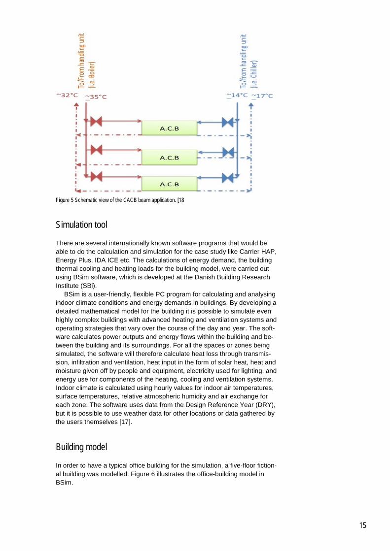
Figure 5 Schematic view of the CACB beam application. [18

Simulation tool

There are several internationally known software programs that would be able to do the calculation and simulation for the case study like Carrier HAP, Energy Plus, IDA ICE etc. The calculations of energy demand, the building thermal cooling and heating loads for the building model, were carried out using BSim software, which is developed at the Danish Building Research Institute (SBi). BSim is a user-friendly, flexible PC program for calculating and analysing indoor climate conditions and energy demands in buildings. By developing a detailed mathematical model for the building it is possible to simulate even highly complex buildings with advanced heating and ventilation systems and operating strategies that vary over the course of the day and year. The soft-ware calculates power outputs and energy flows within the building and be-tween the building and its surroundings. For all the spaces or zones being simulated, the software will therefore calculate heat loss through transmis-sion, infiltration and ventilation, heat input in the form of solar heat, heat and moisture given off by people and equipment, electricity used for lighting, and energy use for components of the heating, cooling and ventilation systems. Indoor climate is calculated using hourly values for indoor air temperatures, surface temperatures, relative atmospheric humidity and air exchange for each zone. The software uses data from the Design Reference Year (DRY), but it is possible to use weather data for other locations or data gathered by the users themselves [17].

Building model

In order to have a typical office building for the simulation, a five-floor fiction-al building was modelled. Figure 6 illustrates the office-building model in BSim.

15

Figure 6 Building geometry in BSim; 1: South view, 2: East view, 3: Top view, 4: 3-D view.

In order to simplify the model, it is assumed that the building is not affect-ed by venting loads due to unconditioned spaces. The venting load pertains to the effect of the air changing between building inside and the outdoors by using an opening like a window. The building construction materials were selected in order to satisfy the minimum acceptable U-value which was indicated in Danish Building Regu-lation (BR10) [5]. The model consists of 78 single office rooms, 5 corridors and 6 meeting rooms. Each office room has a gross area of 12 m2 (net area of 10 m2) and each meeting room is double size of a single office room (approx. 20 m2). Window gross area size defined as 1.6 X 1.6 m2 constant for all windows. Each office room has one external window on each external wall, whereas each meeting room has two. In addition, it was assumed that office rooms are separated from corridors by an internal wall to make the geometry as simpler as possible. This can be imagined as an office room with closed door, where doors have the same U-value as internal walls. Moreover, each corridor has two windows facing east and north. Office rooms were divided into two categories: occupied and unoccupied. The office rooms were supposed to have 50 % occupancy. The occupancy percentage is pertained to the amount of internal loads produced by human metabolism and the amount of heat released to the space by human activity. Therefore, a higher occupancy percentage results in more internal load caused by the occupants and, consequently, it affects the energy demand of the building. For simplification, there are no stairs connecting floors in order to prevent mixing load influences. In addition, the rooms do not have any opening to each other or to the corridors. Hence, there is no air mixing between thermal zones. As mentioned, the U- value was selected as the criterion for building ele-ments. It means that the type of construction material was not considered in the modelling and the U-value was considered for the selection. The U-values were selected in order to meet the minimum requirements of the Dan-ish Building Regulation that can be seen in Table 1 [5].

Building geographical location data The building location was selected in Denmark, where the project was de-fined. Hence, Danish weather data were selected.

16

Building operating hours Below is the operation time schedule for building:

• Working hours: the building working hours were defined as 8:00-17:00 Monday to Friday.

• Non-working hours: They were defined as whole weekends as well as the hours from 00:00-8:00 and 17:00-24:00 of working days.

• Meeting room hour: each meeting room was supposed to be occu-pied from 10:00-11:00 and 14:00-15:00 during working days (Mon-day-Friday).

Building construction data The construction material and element were chosen for each building ele-ment. The elements were obtained from the BSim construction library in BSim database. The U-values of the elements were chosen in order to meet the Danish Building Regulations’ minimum requirements. Table 1 shows an overview of construction element specification.

Table 1 Building model element U-value and Danish Building Regulations’ minimum U-value. [5]

Building Elements

Model U-Value [W/°K.m2]

BR10 minimum acceptable U-value [W/°K.m2]

Roof 0.161 0.2 Floor 0.417 0.5 Ground Floor 0.169 0.2 External Wall 0.251 0.3 Internal Wall 0.418 0.5 Window 1.273 1.8

Building internal load In the modelled building, it was assumed that some elements generated heat during operating hours. The internal heat releases were due to the op-eration of:

• People: it was assumed that the building had 50 % occupancy in the office rooms during the working hours. One person occupied each single office room. Person activity type was selected as Standard that released heat of 100 W. Meeting rooms and corridors were oc-cupied by 6 and 1 person respectively during their operating hours.

• Lighting: it was assumed that the lighting had the power capacity of 7 W/m2 by fluorescent lamps. In addition, in BSim, there was an op-tion that enabled the control of lighting by the lux amount. A refer-ence point was chosen for controlling the lighting. By using the Sim-Light module of BSim, the amount of lux in reference point was cal-culated [17]. Therefore, lighting was ON if the lux value of the refer-ence point became less than the defined value. In the building mod-el, the Reference Point was situated in the middle of the third-floor corridor.

• Equipment: it was presumed that each single office room had some equipment, i.e. a desktop computer, with average power of 150 W. In the corridors, the power of the equipment, i.e. coffee machine etc., was assumed as 600 W during working hours and 400 W con-stant loads, i.e. server room, as Always load. Hence, 1 kW power was selected as equipment power in the corridor which works 100 % in working hours and 40 % in non-working hours. In the meeting rooms, 600 W was selected as the equipment heat generation in each meeting room during the meeting room occupancy hours.

17

HVAC System Model

The HVAC system was modelled as close as possible to the active chilled beams system to obtain energy demand of the building. In order to create a realistic HVAC system for the model, it was presumed that ventilation, heat-ing and cooling systems provided convenient indoor climate for the BSim model. In BSim, there was no cooling system as an active chilled beam. There-fore, for cooling system, it was assumed that the active chilled beam function was similar to a fan coil. For the heating system, BSim did not have a fan coil option as heating system. Thus, it was presumed that the beam could be simulated as a heat-ing radiator. However, there was an option in BSim that made it possible to define the proportion of heat transfer by either radiation or convection de-nominated Part to Air. The Part to Air provides the opportunity for the BSim user to define the proportion of heat transferred by convection. Hence, the Part to Air in BSim gives opportunity to simulate a heating ACB system that transfers heat by mostly (90 %) by convection. Each office room was supposed to be conditioned by one active chilled beam. Additionally, it was assumed that two active chilled beams condi-tioned each meeting room with the double size of a single office room. How-ever, in corridors, one active chilled beam conditioned every 12 m2 of the corridor area. Maximum capacities for heating and cooling devices were selected to be sufficient to provide sufficient heating and cooling energy for the spaces. Hence, the energy demand of the building was desired output data from the BSim simulation to be used in the comparison between the CACB system and the Two-Pipe System.

HVAC operating hours Although the building model was supposed to be occupied from 8:00, the HVAC working hour control system was defined at 7:00. This was assumed in order to reach convenient and defined indoor set point temperatures at 8:00 when people begin working. The HVAC system controlling hours was according to Table 2.

Table 2 HVAC control System. Working Hours Non-work Hours Weekends HVAC system controlling hours 7:00-17:00 00:00-7:00 & 17:00-24:00 00:00-24:00

Thermal zones Building spaces were divided into seven thermal zones. The selection was based on occupancy, geographical direction and usage of the spaces. Table 3 indicates the definition of zones.

Table 3 Thermal zones specifications.

Thermal zones Number of rooms Single office room Gross area [m2]

Total Gross area [m2]

South Occupied 20 12 240 South Unoccupied 19 12 228 South Meeting room 3 24 72 Corridor 5 121.5 607.5 North Occupied 19 12 228 North Unoccupied 20 12 240 North Meeting room 3 24 72

18

The rooms in each thermal zone were selected arbitrarily and discretely in order to get an unbiased room selection and a realistic occupancy model. The occupancy could vary for each building and each simulation. In addition, people can move from room to room for official activities. However, in order to simplify the model, 50 % occupancy for office rooms was selected. Figure 7 demonstrates South Occupied zone.

Figure 7 Red boxes show South view of South Occupied rooms.

Shading system

Table 4 Windows’ shading control.

Shading Maximum lux before curtain down

Minimum lux before C curtain up

Time

Occupied Zone 150000 10000 8:00-17:00 Meeting room 600 200 10-11 & 14-15

Although shading of windows is not generally categorised as HVAC sys-tems, its connection to solar radiation and its control system justified men-tioning specifications in this section. The shading system was defined as an internal curtain with transparency of 50 % for the whole building. Also, the curtain was fully open (the room was dimmed) if the lux amount in the room exceeded the defined value. The curtain control is manually operated and depends on the occupant’s comfort level and the occupant opened /or closed the curtain. Furthermore, the shad-ing was integrated for only occupied zone and meeting room zones while corridors and unoccupied zone were assumed to not be shaded. The control system for the shading system was defined for occupied hours (8:00-17:00) when the occupant manually controls it. Also, it was defined that meeting rooms were shaded during meeting hours 10:00-11:00 and 14:00-15:00. All curtains were up during non-occupied hours. The amount of lux that was de-fined for controlling the shading is listed in Table 4. The lux values for control in the occupied zone were within standard ranges [17]. It should be noted that the meeting rooms’ lux control was de-fined in order to keep the curtain closed during meeting hours since normally the meeting rooms need to be dimmed for presentation. Moreover, all cur-tains in meeting rooms were open during non-working hours.

Ventilation system The ventilation system was assumed to play a role as the primary airflow through nozzles in the active chilled beam system in the model. Constant Air Volume (CAV) was selected as ventilation system. A CAV sys-tem has a constant airflow rate as well as a constant air supply temperature in certain periods. For the ventilation system some general assumptions were made for all thermal zones.

19

Recovery units operated for both cooling and heating recovery with effi-ciency of 90 %. This value indicated that 90 % of the exhaust air energy was recovered in the ventilation recovery unit [14, 15]. Fans released 50 % of heat, generated by their electrical motors, to venti-lation air when they raised the pressure with 250 Pa for each thermal zone. The intake source of air was defined as outdoor in BSim. The airflow rate was assumed to be 25 l/s for each beam. Since it was assumed that one beam was installed in an office room (net area of 10 m2), a 25 l/s airflow rate meets the REHVA range (1.5-3 l/s, floor m2) [12]. Infiltration for each zone was assumed to be 0.2 Air Changing per Hour (ACH). This indicates the tightness of the building envelope. Air supply temperatures are defined in Table 6. In the BSim simulation, the maximum capacity of the cooling and heating coils in AHU should be sufficient in order to supply air due to temperature set point of the ventilation system. The ventilation air temperature, in the active chilled beam system, ranges from 18-20 °C in summer and 19-22 °C in win-ter [12]. Supply-air temperatures, which were assumed, can be found in Ta-ble 6. In order to define estimations of maximum cooling and heating capaci-ty of the Air Handling Unit (AHU), minimum and maximum outdoor air tem-peratures in the year was required. According to the Danish Metrological In-stitute the weather data, which is used in the BSim program, the extreme outdoor air temperature in 2010 was -18 °C and +32 °C during the working hours (7:00-17:00) and -21 °C and +28 °C in non-working hours.

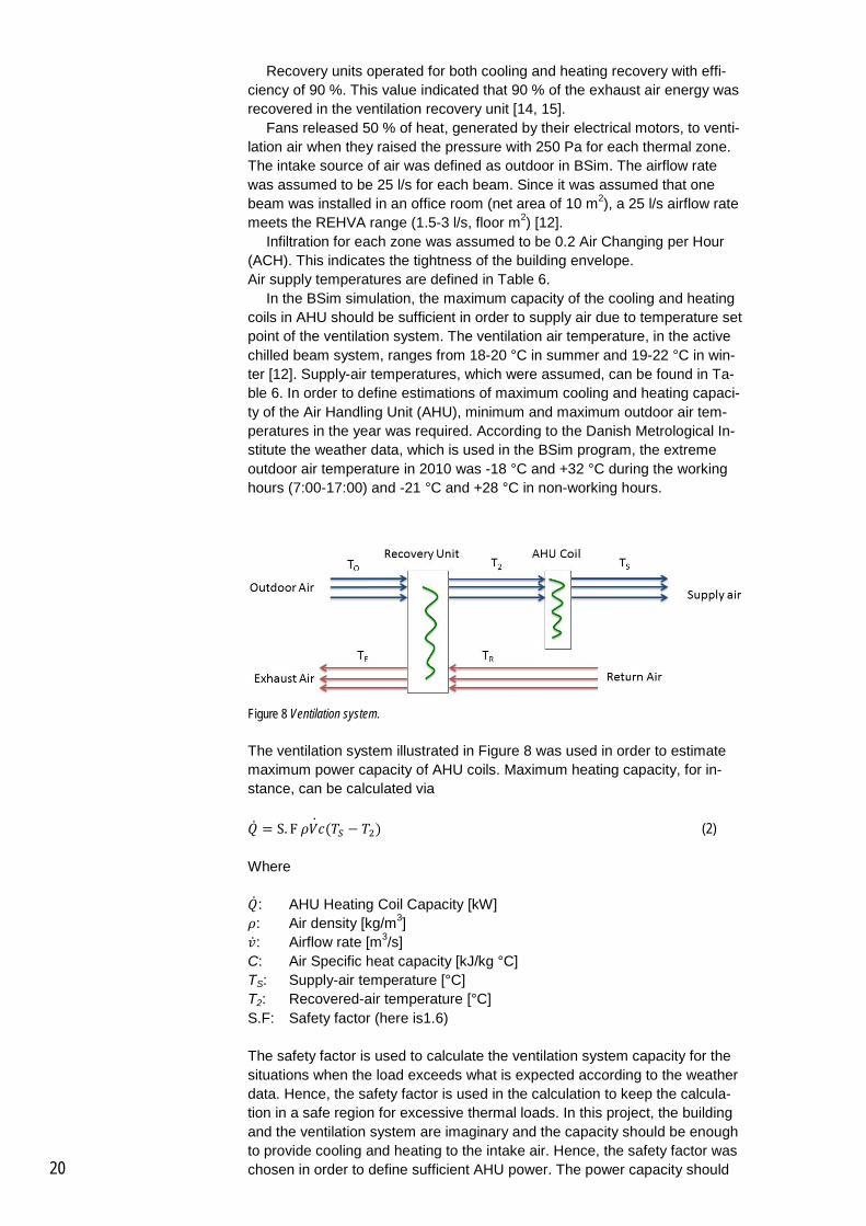
Figure 8 Ventilation system.

The ventilation system illustrated in Figure 8 was used in order to estimate maximum power capacity of AHU coils. Maximum heating capacity, for in-stance, can be calculated via �̇� = S. F 𝜌𝑉𝑐(𝑇𝑆 − 𝑇2)̇ (2)

Where �̇�: AHU Heating Coil Capacity [kW] 𝜌: Air density [kg/m3] �̇�: Airflow rate [m3/s] C: Air Specific heat capacity [kJ/kg °C] TS: Supply-air temperature [°C] T2: Recovered-air temperature [°C] S.F: Safety factor (here is1.6) The safety factor is used to calculate the ventilation system capacity for the situations when the load exceeds what is expected according to the weather data. Hence, the safety factor is used in the calculation to keep the calcula-tion in a safe region for excessive thermal loads. In this project, the building and the ventilation system are imaginary and the capacity should be enough to provide cooling and heating to the intake air. Hence, the safety factor was chosen in order to define sufficient AHU power. The power capacity should

20

be able to provide defined ventilation air temperature to be supplied to the thermal zones. However, in reality, the safety factor should be chosen as close as possible to 1, because it affects the size of the ventilation system directly. It means that if a higher safety factor is used in a calculation, the ventilation system will be bigger and the cost is higher. Furthermore 𝑇2 = 𝜂 × (𝑇𝑅 − 𝑇𝐸) + 𝑇𝑂 (3)

Where T2: Recovered-air temperature [°C] 𝜂: Recovery Unit Efficiency TR: Return air temperature from rooms [°C] TE: Exhaust Air temperature to building outside [°C] TO: Outdoors air temperature (here for maximum power calculation is the

minimum outdoor temperature in the year) [°C] By applying Equations (2) and (3), an estimate of the maximum heating ca-pacity of the AHU coil can be obtained. In addition, the air density and the specific heat capacity of air were assumed to be constant and equal to 1.23 [kg/m3] and 1.0035 [kJ/kg °C] respectively. The air density is dependent on the temperature; 1.2 kg/m3 at 15 °C is chosen as the air density for ventila-tion system calculations [17]. The coldest outdoor temperature of the year during the working hours is -18 °C (=TO). Supply-air temperature in winter was selected as 22 °C (=TS) and it was assumed that the return air temperature (TR) was 23 °C due to human activities, sunlight radiation and heat generation from equipment. Hence, the return air temperature was defined as 23 °C since the room tem-perature in winter is ranged between 22 and 23 °C (see Table 1). The set point temperatures can be found in Table 1. The exhausted air (TE) should be above outdoor dew point temperature to avoid icing on the recovery unit surface. The outdoor dew point was -11 °C when the outdoor temperature was -18 °C and the humidity ratio of exhaust air was 1.4 gwater/kgair by using Mollier-h-x diagram. The diagram can be found in the Appendix 1.The hu-midity ratio is the sum of intake air humidity content (about 0.8 g/kgair accord-ing to Mollier diagram at -18 °C) and office production (about 0.6 gr/kgair [5]). T2 was calculated using Equation (3). T2= 0.9×(23-(-11)) + (-18) =16 °C Consequently, the maximum estimated capacity of the heating coil was cal-culated for South Occupied zone (with 20 rooms and 20 beams) by applying Equation (2). �̇� = 1.6 ∗ 1.23 ∗ (0.025 ∗ 20) ∗ (22 − 16) ≈ 6.17 [𝑘𝑊] For all thermal zones in the model similar calculations were performed and the results can be found in Table 5. It should be considered that the values in Table 1 were calculated in order to have sufficient power in BSim to pro-vide ventilation air with due temperature (according Table 6) and airflow rate. In Table 5 negative values indicate cooling capacity. Flow rate for non-working hours was defined as 40 % of working-hour airflow rate and it was calculated as 25 l/s for each beam unit. Table 6 illustrates the temperature definition for ventilation, cooling and heating systems that were controlled by a specific time schedule.

21

Table 5 Airflow rate and AHU Coils capacity in each zone.

Thermal zone Maximum AHU Heating/cooling Coil power [kW]

Air flow rate [m3/s]

Working hours (07:00-17:00)

Non-Working hours (00:00-07:00 & 17:00-24:00 & Weekend)

South Occupied 6,17/-6,17 0,5 0,2 South Unoccupied 5,85/-5,85 0,475 0,19 South Meeting room 1,8/-1,8 0,15 0,06 Corridor 13,88/-13,88 1,125 0,45 North Occupied 5,85/-5,85 0,475 0,19 North Unoccupied 6,17/-6,17 0,5 0,2 North Meeting room 1,8/-1,8 0,15 0,06

Table 6 Temperatures control for beam simulation.

Winter Spring & Autumn Summer

Time 0-7 7-17 17-24 0-7 7-17 17-24 0-7 7-17 17-24

Air supply 18 22 18 14* 21 18 14* 20 -

Heating 18 22 18 18 21 18 18 20 -

Cooling 22 23 - 21 22 - 20 21 -

Water mean 18.5 22 18.5 18.5 21.5 18.5 18.5 21 - @ Max cooling power

29 32.5 29 29 32 29 29 31.5 -

In Table 6, there are items that should be clarified: • Weekends have same control as non-working hours (17:00-24:00). • Seasons months were defined as:

o Winter: December, January and February o Spring: March, April and May o Summer: June, July and August o Autumn: September, October, and November

• 14* is a specific control that was defined in order to supply 14 °C air

if the outdoor temperature was below 14 °C. Otherwise, if the out-door temperature was above 14 °C, the supply air temperature was assumed to be as outdoor temperature. This was assumed in order to allow outdoor air to be supplied to the zones in autumn, spring and summer and, hence, AHU coils would not operate.

• BSim did not have the ability of simulating heating system as fan coil. Hence, the heating system provided heat to make constant in-door air temperatures line in row Heating in Table 6. However, cool-ing is supplied to the zones when the zone temperature exceeds the set point according to the Cooling row values. Moreover, the zone temperature can rise till @Max. Cooling power row values. The @Max. Cooling power row indicated the maximum zone tempera-ture when the maximum cooling power was supplied to the zones. Thus, for cooling, zones have floating temperatures dependent on cooling power supply.

• All temperatures were defined after examining different possibilities in BSim with the Lindab Comfort A/S cooperation team. Shading ef-fects, air supply temperatures, time schedule for HVAC component

22

operation etc. were examined and several simulations were per-formed to find a down-to-earth control system and, hence, simulation for active chilled beams. Therefore, Table 6 was concluded as the closest possible control system for an active chilled beam.

• During working hours, set point temperatures for air-supply, heating and cooling system were defined, according to REHVA handbook, 18-22 for supply air, 23-26 for cooling and heating [12].

• During non-working hours (00:00-07:00), the HVAC system was controlled to keep the building construction temperature above 14 °C ,which is the lowest allowable temperature for building compo-nents in the Danish Building Regulation [5]. Moreover, the heating and cooling systems operation, during non-working hours (00:00-07:00), helped avoiding high heating /cooling loads on the system at the beginning of working hours (07:00-17:00) to reach convenient set points.

During non-working hours (17:00-24:00), the strategy was to keep the build-ing warm (same as 00:00-07:00) in spring, autumn and winter. Cooling was not required to avoid unnecessary cooling load on the HVAC system after 17:00. The bottom row (@ max. cooling power) in the table indicates the maxi-mum zone temperature when maximum cooling power is supplied to a zone.

Cooling system As mentioned in the limitation of the HVAC system model (page 18), the Fan coil function in BSim was selected to simulate the coil part of an active chilled beam. The fan coil function provides the possibility of defining supply-cooling power as a function of difference between room temperature and cooling fluid (water). Therefore, regarding Table 6, the cooling system con-trol allowed increasing room temperature from its set point (e.g. 21 °C in summer) to the temperature that is defined for maximum cooling power sup-ply (e.g. 31.5 °C for summer). The measurement results [22] indicated that application of an active chilled beam, with the power of 530 W, corresponds to having almost 3 °C temperature gradient between the water inlet and out-let and the room temperature is kept almost 3.5 °C above water mean tem-perature. In order to have enough cooling system capacity, 1590 W were assumed as one beam maximum cooling power which is 3 times more than the actual power of the measured ACB. Table 7 indicates the maximum heating/cooling power capacity of each zone. Moreover, an ACB system exchanged heat mostly by convection since ventilation and induced air pass over the beam coil. A mixture of induced air and the ventilation air provided heating or cooling for the spaces. However, a small proportion of the exchanged heat was due to radiation when there were two surfaces with different temperatures. In order to model a realistic active chilled beam system in the BSim simulation, it was assumed that fan coils (ACBs) cooled spaces by 90 % convection (and 10 % radiation) that could be defined in Part to Air. The main purpose of the BSim simulation was to obtain the model thermal loads in order to compare the energy use of the two active chilled beam sys-tems. Furthermore, maximum capacity of cooling and heating systems do not affect the thermal demand of the model although the capacity should be defined sufficiently in order to provide adequate cooling or heating power to keep the space temperature according to Table 6. The cooling and heating demand of a space depends on parameters such as human activity, solar radiation, heat generated by equipment, lighting etc. Thus, the capacity of the cooling or heating system does not influence thermal demand of the space. In corridors, since there was no significant internal heat generation (i.e. people), the cooling and heating maximum capacities were assumed to be -9 and 4 kW respectively for each corridor.

23

Table 7 Active chilled beam Heating/Cooling maximum power.

Thermal zone ACB Heating/Cooling Power [kW]

South Occupied 31.8/-31.8 South Unoccupied 30.2/-30.2 South Meeting room 9.54/-9.54 Corridor 20/-45 North Occupied 30.2/-30.2 North Unoccupied 31.8/-31.8 North Meeting room 9.54/-9.54

Heating system The heating system functionality, in the simulation, was selected to be a ra-diator. However, as it was mentioned in the HVAC limitations (Page 18), BSim user is able to determine the convection proportion of heat transfer by the heating device (in this case a radiator). In the simulation, the convection proportion (Part to Air) was defined as 90 %. It reflected that the heating sys-tem operated as a heating fan coil with such assumptions. Radiation and conduction were assumed to cover 10 % of the heat transfer by the heating system. Thus, such a heating system with the combination of CAV ventila-tion system could be a reasonable simulation of an active chilled beam for the heating system. In addition, the temperature control could be found in Table 6 for the HVAC model as well as heating controls. Moreover, the maximum capacity of heating system was documented in Table 7.

Calculation methods

The calculation methods were divided into two parts. One considered the calculation of energy saving due to energy transfer in the Two-Pipe System. Another part focused on a calculation method for when free cooling was ap-plied to the Two-Pipe System and the CACB. Regarding (Page 13), the Two-Pipe System had an inherent characteristic for energy transfer while two-pipes are used for both cooling and heating. Hence, it should be noted that in the second part of the free cooling calculation, the energy transfer effect was taken to account for the Two-Pipe System, while different scenarios for free cooling was applied. Moreover, the calculation for free cooling and heat transfer can be found in the appended CD and Excel file.

Calculation method of energy transferring by the Two-Pipe System In this section, a calculation method of energy transfer by the Two-Pipe Sys-tem concept is described. As mentioned, the Two-Pipe System is expected to have the ability to transfer heat between spaces with cooling demand and spaces with heating demand. In order to calculate the amount of transferred energy and compare it with the CACB, an hourly load calculation was needed. If the total yearly demand was divided by three categories, see Figure 9, the Two-Pipe System was able to take advantages of hours when heating and cooling are demanded simultaneously. But, the energy demand of the Two-Pipe System in the two other catego-ries, heating only (mostly winter) and cooling only (mostly summer), will be the same as the CACB since there were no other sources in the building to transfer energy between different thermal zones. In the Two-Pipe System, the total energy demand was calculated via Equation 4:

24

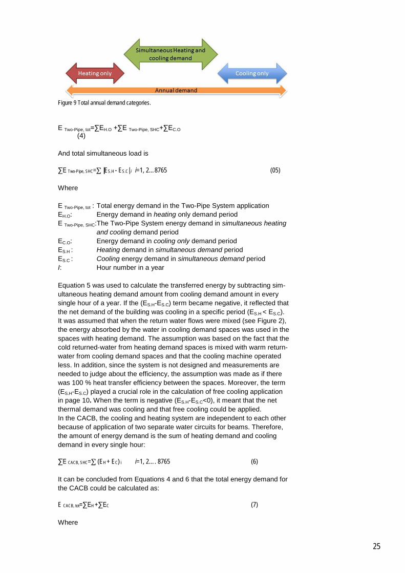
Figure 9 Total annual demand categories.

E Two-Pipe, tot=∑EH.O +∑E Two-Pipe, SHC+∑EC.O

(4) And total simultaneous load is ∑E Two-Pipe, SHC=∑ |ES.H - ES.C| i i=1, 2…8765 (05)

Where E Two-Pipe, tot : Total energy demand in the Two-Pipe System application EH.O: Energy demand in heating only demand period E Two-Pipe, SHC:The Two-Pipe System energy demand in simultaneous heating and cooling demand period EC.O: Energy demand in cooling only demand period ES.H : Heating demand in simultaneous demand period ES.C : Cooling energy demand in simultaneous demand period I: Hour number in a year Equation 5 was used to calculate the transferred energy by subtracting sim-ultaneous heating demand amount from cooling demand amount in every single hour of a year. If the (ES.H-ES.C) term became negative, it reflected that the net demand of the building was cooling in a specific period (ES.H < ES.C). It was assumed that when the return water flows were mixed (see Figure 2), the energy absorbed by the water in cooling demand spaces was used in the spaces with heating demand. The assumption was based on the fact that the cold returned-water from heating demand spaces is mixed with warm return-water from cooling demand spaces and that the cooling machine operated less. In addition, since the system is not designed and measurements are needed to judge about the efficiency, the assumption was made as if there was 100 % heat transfer efficiency between the spaces. Moreover, the term (ES.H-ES.C) played a crucial role in the calculation of free cooling application in page 10. When the term is negative (ES.H-ES.C<0), it meant that the net thermal demand was cooling and that free cooling could be applied. In the CACB, the cooling and heating system are independent to each other because of application of two separate water circuits for beams. Therefore, the amount of energy demand is the sum of heating demand and cooling demand in every single hour: ∑E CACB, SHC=∑ (EH + EC) i i=1, 2…. 8765 (6)

It can be concluded from Equations 4 and 6 that the total energy demand for the CACB could be calculated as: E CACB, tot=∑EH +∑EC (7)

Where

25

E CACB, SHC: The CACB energy demand in simultaneous heating and cooling demand hour E CACB, tot: Total energy demand in the CACB EH: Heating energy demand in any single hour EC: Cooling energy demand in any single hour Thus, the total yearly energy demand for the CACB was calculated using Equation 7, which indicated the independent heating and cooling demand summation. In comparison, the amount of energy saving due to the heat transfer characteristic of the Two-Pipe System was calculated via: Energy saving (%) = [1- E Two-Pipe, tot ÷ E CACB, tot] ×100 (8)

Calculation of free cooling In this section the method in which free cooling was applied to the Two-Pipe System and the CACB is presented. Free cooling is intended to take advantage of the outdoor temperature as a cold source providing cooling for spaces. Therefore, it depends on outdoor temperature and the water supply temperature. For the calculation, it was presumed that free cooling could apply to the building model in five different scenarios (methods) to draw a reasonable picture of its application. The scenarios were based on supply-water temperature for each system, either the CACB or the Two-Pipe System. As mentioned in the background, in the CACB system supply water temperature (for cooling) ranged between 14 °C and 17 °C and the Two-Pipe System was expected to run with a water tem-perature ranging between 20 °C and 23 °C. For simplification, it was as-sumed that water-supply temperatures are 14 °C and 20 °C for the CACB and the Two-Pipe System respectively. Depending on the method for obtaining free cooling, the gradient between outdoor temperature and supply water is different. According to a technical interview with G. Hultmark, R & D manager in Lindab Comfort A/S [19] if a common air-cooled heat exchanger was used for providing free cooling, 6 °C difference between outdoor air temperature and beam-water inlet temperature was reasonable in order to provide 100 % free cooling. Figure 10 indicates the air-cooled heat exchanger which pro-vides cold water for ACBs when the outdoor air temperature is 6 °C less than inlet water temperature. Scenarios 3 and 4 were based on such a sys-tem. In scenario 3, 100 % free cooling is obtained when the outdoor temper-ature was 6 °C less than the inlet water temperature of ACBs (14 °C for the CACB and 20 °C for the Two-Pipe System). Otherwise, if the difference was less than 6 °C, a cooling machine (i.e. chiller) provided cold water.

26

Figure 10(a) free cooling scenario 3 for the Two-Pipe System (b) free cooling scenario 3 for the CACB system.

Scenarios 1 and 2 are based on a method that the outlet water from the beam is cooled down by an air-cooled heat exchanger too. In this method, the water outlet is cooled down by direct airflow provided by a fan but the heat exchanger has larger heat transfer surface and more efficient in heat transfer than the heat exchanger in scenarios 3 and 4. Figure 11 illustrates the performances of scenarios 1 and 2. Instead of 6 °C temperature differ-ence to provide 100 % free cooling in scenarios 3 and 4 (Figure 11), a 4 °C gradient was assumed to be sufficient to obtain 100 % free cooling in sce-narios 1 and 2 [19] Scenario 1 is similar to scenario 3 and scenario 2 is similar to scenario 4. The only difference is the temperature differences for providing 100 % free cooling. The difference between inlet and out let water temperatures in the active chilled beam is 3-4 °C [16]. For simplification, it was assumed that the differ-ence is 4 °C. Consequently, in scenario 2, when the outdoor temperature is 10-11 °C for the CACB and 16-17 °C for the Two-Pipe System, the air-cooled heat exchanger can cool return water to 15 °C in the CACB and to 21 °C in the Two-Pipe system (with respect to 4 °C temperature difference). Hence, the cooling machine (i.e. chiller) operates to cool the water 1 °C (15 °C to 14 °C for the CACB system and 21 °C to 20 °C for the Two-Pipe Sys-tem). The energy is needed to cool 1 °C was 1/4 (25 %) of the full-load op-eration of the cooling machine. The full-load operation was when the cooling machine cools outlet water from 18 °C to 14 °C (cools 4 °C) in the CACB and from 24 °C to 20 °C in the Two-Pipe System. Figure 12 shows schemat-ic view for when 75 % free cooling was obtained in scenario 2.The same idea was applied to 50 % and 25% for the CACB and the Two-Pipe System but with different ranges of outdoor temperatures.

27

Figure 11(a) free cooling scenario 1 for the Two-Pipe System (b) free cooling scenario 1 for the CACB system.

Figure 12(a) 75 % free cooling in scenario 4 for the Two-Pipe System (b) 75 % free cooling scenario 4 for the CACB.

28

For the CACB system, when the outdoor temperature is 11-12 °C, the air-cooled heat exchanger can cool the outlet water from the beam to 16 °C (with respect to 4 °C temperature difference in scenario 2) and the chiller will cool the water from 16 °C to 14 °C for the CACB that is 50% of full-load. Scenario 5 is based on the development perspective regarding heat ex-changers. In this scenario it was assumed that 2 °C difference (between outdoor air temperature and inlet water temperature) can provide 100 % free cooling for both systems. The concept is similar to scenarios 2 and 4 but with a different temperature difference. This scenario is the vision of future efficient heat exchangers. The exchanger in this scenario was assumed to have a capacity that can cool down water to only 2 °C more than the supply air. Table 8 shows the different scenarios.

Table 8 Scenarios 1-5 for free cooling application.

Scenario No. 1 2 3 4 5

Free cooling (%) Outdoor Temperature [°C]

CACB

100 ≤10 ≤10 ≤8 ≤8 ≤12 75 - 10-11 - 8-9 12-13 50 - 11-12 - 9-10 13-14 25 - 12-13 - 10-11 14-15

Two-Pipe System

100 ≤16 ≤16 ≤14 ≤14 ≤18 75 - 16-17 - 14-15 18-19 50 - 17-18 - 15-16 19-20 25 - 18-19 - 16-17 20-21

Scenarios were defined briefly as:

• Scenario 0: No free cooling is applied, neither to the Two-Pipe Sys-tem nor to the CACB. The cooling machine provides 100 % of the cooling demand energy.

• Scenario 1: Free cooling is applied as ON/Off switching mode when the outdoor temperature exceeds specific temperatures (10 °C for the CACB and 16 °C for the Two-Pipe System)

• Scenario2: Free cooling is applied step by step. Free cooling appli-cation percentage decreases from 100 % to 25 % when outdoor temperature rises. (For the CACB 10-13 °C and for the Two-Pipe System 16-19 °C)

• Scenario 3: Free cooling is applied like in scenario 1, but the specif-ic temperatures are different. (8 °C for the CACB and 14 °C for the Two-Pipe System)

• Scenario 4: Free cooling is applied like in scenario 2, but tempera-ture ranges are different (the CACB 8-11 °C, the Two-Pipe System 14-17 °C)

• Scenario 5: Free cooling is applied like in scenario 2, but tempera-ture ranges are different (the CACB 12-15 °C, the Two-Pipe System 18-21 °C). This scenario was defined for future development scopes. It was expected to design and develop a free cooling sys-tem in order to have 100 % free cooling when the outdoor tempera-ture is 2 °C lower than inlet water temperature in the Two-Pipe Sys-tem and the CACB systems (when the outdoor temperature is 18 °C for the Two-Pipe System and 12 °C for the CACB application). The free cooling percentage is diminished to 75, 50 and 25 % when out-door temperature rises. (See Figure 12 and the text above it)

Considering Equation 7, free cooling applied to the EC in the CACB. Mean-while, for Equation 4, free cooling is applied to EC.O and negative values of

29

(ES.H – ES.C) term, in Equation 5, in Two-Pipe System. Because negative val-ues of the term indicated that the overall simultaneous demand was cooling and, hence, free cooling could be applicable. On the other hand, all temperature definitions in scenarios 1-5 were applica-ble for all cooling demands (EC in Equation 7), independently of heating, in the CACB during a year. It means that since there is no effect of heat trans-fer in the CACB system and there are two separate circuits for cooling and heating, free cooling scenarios are applied to each cooling demand regard-less of whether there is any heating demand simultaneously in the building. In the Two-Pipe System, in order to calculate the amount of possible en-ergy transfer between cooling demanding spaces and heating demanding spaces, the term (ES.H – ES.C) was used, which meant the difference between cooling demand in one space and heating demand in another space. If the term becomes negative (ES.H < ES.C), it means that the net demand (after transferring energy) for whole building is cooling.

30

Result

Simulation in BSim provided an adequate building energy demand calcula-tion that enables comparison between two active chilled beam systems. Output data from BSim, which were needed for the investigation in this pro-ject, are hourly cooling, heating and ventilation loads. The simulation gave results for the CACB since the heating system and cooling system were de-fined independently in BSim. However, in the Two-Pipe System, the cooling and heating systems operate within one two-pipe system and are dependent on each other. The calculation methods in section free cooling (Page 10) were applied to raw output data from BSim, which are hourly heating and cooling demands of the building model, to calculate the Two-Pipe System energy use too. Generally, the building-model load balance in 2010, which was selected as year for weather database in BSim, is represented in Figure 13. Figure 13 illustrates the yearly energy demand in the air handling unit (AHU) and beam cooling and heating systems. In AHU, the energy demand is due to heating and cooling coils and ventilation fan. Cooling coil, heating coil and fan energy demand are 1.4, 8.6 and 6.8 kWh/m2 respectively. On the other hand, beam heating (26.7 kWh/m2) and cooling (15 kWh/m2) loads were cal-culated in BSim. In the appended CD, there is an Excel file that represents hourly BSim load calculations. The energy demand dimension was defined as kWh/m2 in the figure to give an image of energy demand per area unit in the building model. The amount of the energy demand for heating, cooling and ventilation is in the acceptable region of the Danish Building Regulations [5]. Table 9 indicates the energy balance in a year. The output data from BSim represents balanced energy in the building model since the sum of all values is zero. Therefore, the capacity of ventilation system, cooling system and heating system were sufficient to cover the thermal loads of the building model and to provide defined indoor temperatures according to Table 6.

Figure 13 Annual energy demand in building model from BSim software.

15.0

26.7

6.8 1.4

8.6

0

10

20

30

40

50

60

70

Ener

gy D

eman

d [k

Wh/

m2 ]

AHU Heating coil

AHU Cooling coil

AHU Fan Energy

Beam Heating

Beam cooling

31

Table 9 Building model Energy Balance.

Building mod-el

Energy [kWh/m2]

Comment [17]

QHeating 26.7 Energy used for heating in the thermal zone, kWh.

QCooling -15 Energy used for cooling (negative) in the thermal zone

QInfiltration -19.5 Energy added (+) or removed (-) by infiltration of air from the ambient to the thermal zone, kWh

QVenting 0 Not applicable

QSunRad 37.4 Energy from solar radiation through WinDoors (windows and/or doors) in the thermal zone minus solar radiation which is lost before it enters the zone, and minus solar radiation that passes on to other rooms

QPeople 8.5 Energy from persons in the thermal zones

QEquipment 19.2 Energy used for equipment in the thermal zones

QLighting 9.3 Energy used for artificial lighting in the thermal zones

QTransmission -44.3 Energy transferred (positive or negative) by transmission through the con-structions and WinDoors of the thermal zones

QMixing 0 Not applicable

QVentilation -22.4 Energy transferred (positive or negative) by air-transport through the venti-lation system in the thermal zones- incl. energy used in the components of the ventilation system (heating coil, cooling coil, etc.)

Sum 0

In addition, in order to compare the Two-Pipe System and the CACB energy use, energy demand in Beams (26.7 and 15 kWh/m2) should be considered for comparison. Ventilation loads are equal and constant in the CACB and the Two-Pipe System. Scenarios, in section free cooling (Page 10), were applied to BSim output. The Figure 14 shows the amount of total yearly energy demand calculated through each scenario for the CACB and the Two-Pipe System concepts. It can be seen that annual demand of the Two-Pipe System is 56.59 kWh/m2 and the annual demand of the CACB system is (26.7+15+6.8+1.4+8.6=) 58.44 kWh/m2 when there is no free cooling appli-cation.

Figure 14 total energy demand in different scenarios, Two-Pipe System vs. CACB.

58,4

4

57,1

4

56,5

9

57,6

9

57,2

9

55,1

8

56,5

9

50,0

9

49,1

3

52,3

1

51,8

8

45,6

0

0,00

10,00

20,00

30,00

40,00

50,00

60,00

70,00

Scen

ario

0

scen

ario

1

Scen

ario

2

Scen

ario

3

Scne

ario

4

Scen

ario

5

Bui

ldin

g A

nnua

l Ene

rgy

Dem

and

[kW

h/m

2]

CACB (Four-PipeSystem)

Two-Pipe System

32

For in-depth load calculations of each scenario, Figure 20 provides a de-tailed version of Figure 14. In Figure 20, all air handling unit (AHU) values are constant values in the CACB and the Two-Pipe systems, because, the new Two-Pipe System pertains only to the beam part of the HVAC system, where the water-flow in the beam coil conditions the space, and the ventila-tion system and parameters are constant while the CACB system is com-pared to the Two-Pipe System. The ventilation loads are taken to account in order to calculate and compare the total annual building demand for both systems. Therefore, the energy transfer effect and the free cooling effect are applied to ACB Simultaneous heating and cooling, ACB Heating and ACB Cooling of the Figure 20 and the AHU values are only repeated as constant values in each bar chart. In addition, in order to compare energy demand in two systems, ACB Heating and ACB Cooling in the CACB bar charts should be compared with three bar charts in the Two-Pipe System that are the ACB Heating, the ACB Cooling and the ACB Simultaneous heating & cooling. In scenarios 1-5 free cooling was applied to ACB Cooling bars in the Two-Pipe System and the CACB system. Moreover, in Simultaneous heating and cooling demand hours in the Two-Pipe System, free cooling was applied to those hours when the amount of cooling demand are higher than heating demand ((ES.H-ES.C)<0). Figure 16 shows the annual cooling energy demand in the model. The comparison was made between the Two-Pipe System and the CACB by im-plementing different scenarios.

Figure 15 Yearly Energy Demand for the Two-Pipe System vs. the CACB.

0

10

20

30

40

50

60

70

CA

CB(

Four

-Pip

e Sy

stem

)Tw

o-P

ipe

Sys

tem

CA

CB(

Four

-Pip

e Sy

stem

)Tw

o-P

ipe

Sys

tem

CA

CB(

Four

-Pip

e Sy

stem

)Tw

o-P

ipe

Sys

tem

CA

CB(

Four

-Pip

e Sy

stem

)Tw

o-P

ipe

Sys

tem

CA

CB(

Four

-Pip

e Sy

stem

)Tw

o-P

ipe

Sys

tem

CA

CB(

Four

-Pip

e Sy

stem

)Tw

o-P

ipe

Sys

tem

Yea

rly E

nerg

y de

man

d [k

Wh/

m2 ]

AHU Fan

AHU Cooling Coil

AHU Heating Coil

ACB Heating

ACB Simultaneousheating & cooling

ACB Cooling

33

Figure 16 Annual cooling energy demand; Two-Pipe System vs. CACB in different scenarios.

In order to show maximum zones temperature in cooling when the beams (fan coils option in BSim) were operating with maximum defined power, the Table 10 illustrates when the maximum cooling power was sup-plied to each thermal zone. It also indicates the room temperature as well as the set point temperature that was introduced in Table 6. Table 10 indicates the time and amount of the maximum cooling demand of each thermal zone is in building model. Moreover, it indicates the cooling set points, which were defined in Table .6, and the room operational temper-atures for when the maximum cooling demands occur. The difference be-tween the room temperature and the set point temperatures is due to the fan coil function in BSim in which the room temperature was controlled as a function of maximum cooling power of the beam. Figure 17 shows that the room temperature rises while the cooling power supply increases.

Figure 17 Corridor air temperature [°C] control by supply-cooling power [kW].

16,3

3

15,0

3

14,4

7

15,5

7

15,1

7

13,0

7

15,4

0

10,2

0

7,94

12,7

4

10,6

9

5,56

0,002,004,006,008,00

10,0012,0014,0016,0018,00

Sce

nario

0

scen

ario

1

Sce

nario

2

Sce

nario

3

Scn

eario

4

Sce

nario

5Ann

ual C

oolin

g En

ergy

Dem

and

[k

Wh/

m2]

CACB (Four-Pipe System)

Two-PipeSystem

34

Table 10 Maximum cooling load and room temperature.

Thermal zone

Maximum cool-ing demand [kW]

Time

[yyyy.mm.dd hh:mm]

Room tempera-ture [°C]

Set point tempera-ture

[°C]

South Oc-cupied

In working hour (7-17) 8,65 2010.06.07 13:00 23,25 21

In whole year 10,39 2010.08.23 01:00 23,49 20

South Un-occupied

In working hour (7-17) 7,8 2010.08.23 13:00 23,29 21

In whole year 9,37 2010.08.23 01:00 23,37 20

South Meeting room

In working hour (7-17) 3,4 2010.08.23 15:00 23,67 21

In whole year 3,4 2010.08.23 15:00 23,67 21

Corridor

In working hour (7-17) 8,38 2010.06.07 17:00 22,53 21

In whole year 8,38 2010.06.07 17:00 22,53 21

North Oc-cupied

In working hour (7-17) 6,4 2010.06.07 17:00 22,74 21

In whole year 6,4 2010.06.07 17:00 22,74 21

North Un-occupied

In working hour (7-17) 3,57 2010.06.07 07:00 21,9 21

In whole year 5,29 2010.07.12 01:00 22,26 20

North Meeting room

In working hour (7-17) 2,52 2010.06.07 11:00 23 21

In whole year 2,52 2010.06.07 11:00 23 21

35

It can be seen in Figure 17 that corridor cooling system starts to cool the thermal zone when the zone temperature exceeds 22 °C (defined in ble 6). Thermal zone temperature rises to the maximum temperature (row @max. cooling power in Table 6) that the maximum cooling power (defined in Table 7) is supplied to the thermal zone. Therefore, the cooling-power supply increases as well as the zone temperature till maximum cooling ca-pacity. The same cooling control is applied to the six thermal zones in the building model. In Table 10, corridors maximum cooling power in working hours is -8.38 kW. According to Figure 17, the thermal zone temperature with -8.37 kW cooling power supply is around 23 °C. The thermal zone operational tem-peratures can be found in the column room temperature in Table 10. In the heating system the set point temperature is the same as the ther-mal zone operational temperature. Maximum heating loads can be found in the Appendix 1.

36

Discussion

Simulation in BSim was carried out with assumptions in order to simplify the fictional office building. It was assumed that the occupancy was 50 % for of-fice rooms. The building occupancy can be different, but for simplification 50 % was selected as the base of the load calculation. Moreover, it was as-sumed that the building was not affected by thermal load from air-mixing and it was assumed that the building was not affected by thermal load from open windows and natural ventilation. The thermal load was the same for the Two-Pipe System and for the conventional active chilled beam system. In the comparing process it was assumed that the Two-Pipe System could transfer energy while there are simultaneous heating and cooling de-mands in the building. The energy transfer was calculated through the term (ES.H-ES.C) that subtracts the amount of simultaneous cooling demand from simultaneous heating demand in any single hour. This implies that in the Two-Pipe System water absorbs heat in the cooling beam and transfers the heat to the space that needs heating (heating beam). The efficiency of the system was assumed to be 100 % when it transfers heat between spaces and heat losses thorough pipes is neglected. The Two-Pipe System performance for transferring energy is presented in Figure 18. According to the BSim simulation output, on 16th of February be-tween 12:00 and 13:00 the South Occupied zone had a cooling demand of 2.52 kWh with inlet water temperature of 23 °C. At same time the North Un-occupied zone had a heating demand of 5.67 kWh.

Figure 18 Schematic view of simulated energy transfer on 16th February 12:00-13:00.

Both zones have 20 rooms and 20 beams. In addition, the water-flow rate is assumed to be 0.042 l/s (≈0.042 kg water/s) for each beam. Therefore, the return water temperature from each zone can be calculated as:

𝑇𝑟,𝑆.𝑂 = 𝑇𝑖𝑛 +𝐸𝑆.𝐶ℎ

�̇�∙𝑛∙𝐶𝑝= 23 +

2.521

0.042×20×4.18= 23.71 (8)

𝑇𝑟,𝑁.𝑈 = 𝑇𝑖𝑛 −𝐸𝑆.𝐻ℎ

�̇�∙𝑛∙𝐶𝑝= 23 +

5.671

0.042×20×4.18= 21.38 (9)

Where

37

𝑇𝑟,𝑆.𝑂: Return water temperature in the South Occupied zone [°C] 𝑇𝑟,𝑁.𝑈: Return water temperature in the North Unoccupied zone [°C] 𝑇𝑖𝑛: Water inlet temperature [°C] 𝐸𝑆.𝐶: Simultaneous cooling demand [kWh] 𝐸𝑆.𝐻: Simultaneous heating demand [kWh] ℎ: Number of hours [h] �̇�: Water flow rate [kg/s] 𝑛: Number of beams in each zone 𝐶𝑝: Specific heat capacity of water [kJ/kg ° C] The water mixture is the average of both return water temperatures which is 22.54 °C. thus, the handling machine (i.e. boiler) has to warm the return flow from 22.54 °C to 23 °C that corresponds to 3.15 kWh energy {=0.042 • 2 • 20 • 4.18 • 1/(23-22.54)} that is equal to 𝐸𝑆.𝐻 − 𝐸𝑆.𝐶. In the CACB system with two individual cooling and heating circuits the heat-ing energy and cooling energy are provided individually and is equal to 8.19 kWh (= 𝐸𝑆.𝐻 + 𝐸𝑆.𝐶). The free cooling system efficiency does not affect the comparison of the two systems as the efficiencies are assumed equal (100%) in order to be able to compare the two systems with different inlet water temperatures. The two-pipe system is based on having no regulation of the flow in the beam coil, e.g. thermal sensors. Having no regulation valve and individual temperature control can be considered a disadvantage and the annual pumping energy increases for running the system 24 hours in a day. How-ever, in the CACB system regulation valves and temperature sensors control the water circulation in heating or cooling circuits. This section focuses on the results and clarifies energy use in the building model. There are two main subjects that are going to be discussed in this section. First, Scenario 0 represents the energy transfer benefit that the Two-Pipe System has over the CACB. Second, the effect of heat transfer as well as free cooling application in Two-Pipe System and the CACB are dis-cussed through scenarios 1-5. Scenario 0 (first bar) in Figure 19 indicates the total energy saving in the Two-Pipe system through energy transfer between zones. The figure is de-rived from Figure 14 by subtracting the CACB energy demand from the Two-Pipe System energy demand in each scenario. The amount of saved energy is 1.85 kWh/m2 corresponding to about 3.17 %, cf. Figure 20. The net area of the building is 1429 m2 and the energy saved for the building is about 2500 kWh per year.

Figure 19 Annual total energy saving through energy transfer in Two-Pipe System vs. CACB.

1,85

5,75 7,46

3,76 5,41

8,44

0,00

1,00

2,00

3,00

4,00

5,00

6,00

7,00

8,00

9,00

Sce

nario

0

Sce

nario

1

Sce

nario

2

Sce

nario

3

Sce

nario

4

Sce

nario

5

Ann

ual T

otal

Ene

rgy

Savi

ng

[kW

h/m

2]

38

Figure 20 Percentage of energy saved by using the Two-Pipe System vs. the CACB.

The amount of cooling energy saved is shown in Figure 21. The first bar (Scenario 0) shows the amount of cooling energy saved by mean of heat transfer (and no free cooling application). The Two-Pipe System needs 5.6 % less cooling energy than the CACB system. It is noticeable that the energy-transfer-saving potential in the Two-Pipe System is directly dependent on those hours that some thermal zones need cooling while the other zones need heating simultaneously. Therefore, if the amount of simultaneous heating and cooling demands increases, the Two-Pipe System will save energy through greater energy transfer.

Figure 21 Annual cooling energy saving percentage for Two-Pipe System vs. the CACB.

3,17

10,07 13,18

6,51 9,44

15,29

0,00

2,00

4,00

6,00

8,00

10,00

12,00

14,00

16,00

18,00

Sce

nario

0

Sce

nario

1

Sce

nario

2

Sce

nario

3

Sce

nario

4

Sce

nario

5

Ann

ual T

otal

Ene

rgy

Savi

ng

[%]

5,67

32,12

45,14

18,18

29,54

57,48

0,00

10,00

20,00

30,00

40,00

50,00

60,00

70,00

Sce

nario

0

Sce

nario

1

Sce

nario

2

Sce

nario

3

Sce

nario

4

Sce

nario

5

Ann

ual C

oolin

g En

ergy

Sav

ing

[%]

39

Saving due to energy transfer and free cooling In almost all cooling systems, there is an incentive to use cold outdoor air as a free cooling source. In scenarios 1-5 different methods of achieving free cooling energy are investigated for both the Two-Pipe System and the CACB systems. Scenarios 1-5 (Blue bars) in Figure 19 illustrate the amount of energy saved as a result of energy transfer and use of free cooling in the Two-Pipe System compared to the CACB. The amount of energy saved varies be-tween 3.7 and 8.44 kWh/m2 depending on different scenarios of using free cooling corresponding to 6.5-15 % annual energy saving as shown in Figure 20. The amount of energy needed to cool the building through out a year is compared in Figure 21 by scenarios 1-5. It can be seen that by applying free cooling the Two-Pipe System needed 18-57 % less cooling energy annually than the CACB system. High temperature in the Two-Pipe System for cooling as well as energy transfer in the Two-Pipe System results in up to 15 % energy saving com-pared with the CACB system. Since the Two-Pipe System uses a two-pipe system for supply and return water it needs less piping material than a four-pipe system (CACB). This re-sults in less construction costs too. Moreover, regulation valves are not needed for each chilled beam to regulate cold water and hot water because the water temperature ranges between 20 °C and 23 °C which can provide both cooling and heating when needed.

40

Conclusion

The simulations and the calculations showed that the Two-Pipe Active Chilled Beam System has the potential of saving energy in different ways. The Two-Pipe System has the potential of transferring energy between spaces where there is a cooling demand and spaces where there is a heat-ing demand. Since the Two-Pipe System uses higher water temperatures for cooling, it gives a wider range of outdoor air temperature that can be used as a free cooling source. Through comparing the simulated energy use in the Two-Pipe System and in a conventional active chilled beam system it is found:

• In the Two-Pipe System energy transfer between spaces is ex-pected to save 1.85 kWh/m2. This amount is equal to 3 % of the en-ergy that the conventional active chilled beam system uses annually. In addition, energy-transfer characteristic in the Two-Pipe System enables 5.6 % saving of total annual cooling energy needed in the conventional active chilled beam system.

• Different free cooling scenarios (methods) for the Two-Pipe System and the conventional active chilled beam system, as well as energy transfer performance of the Two-Pipe System showed that the ener-gy use can be reduced by 3.7-8.5 kWh/m2 which corresponds to about 7-15 %. Consequently, energy used for cooling can be re-duced by 18-57 %.

41

References

[1]http://www.lindab.com/global/pro/Pages/default.aspx?redirectToMarket=true&i=8301#drilldown_guid:4825115a-d5c4-4bd6-8158-78aa115303b0;level:all;sub:4 [accessed 12 Dec. 2012] [2] RUMSEY P. “Chilled Beams”, Heating/Piping/Air Conditioning Engineer-ing. (2010), 82(1): 46-49. [3] American Society of Heating, Refrigerating and Air-Conditioning Engi-neers. “2011 ASHRAE Handbook: Heating, Ventilating, and Air-Conditioning Applications”. Atlanta, Ga: ASHRAE, 2011. Ch. 57.12. [4] Rumsey P, Rumsey F, Weale J. “Practical Implementation of Chilled Beams For Offices”, Engineered Systems. (2011), 28(1): 30-36. [5] The Danish Ministry of Economic and Business Affairs. Danish Enterprise and Construction Authority, “Building Regulations 2010, BR10”, Copenhagen 2010. [6] Livchak A, Lowell C. “Don't Turn Active Beams into Expensive Diffusers”, ASHRAE Journal. (2012), 54(4): 52-60. [7] Alexander D, O'Rourke M. “Design Considerations For Active Chilled Beams”, ASHRAE Journal (2008), 50(9): 50-58 [8] Roth K, Dieckmann J, Zogg R, Brodrick J. “Chilled Beam Cooling”. ASHRAE Journal. (2007), 49(9): 84-86. [9] Steve P. Doty, PE, CEM. “Simultaneous Heating and Cooling -The HVAC Blight”, Energy Engineering. (2009) 106(2):42 – 74. [10] Loudermilk K. “DESIGNING Chilled Beams FOR Thermal Comfort”. ASHRAE Journal. (2009), 51(10): 58-64. [11] Pope K. “New Tech, Old Buildings”. Environmental Design & Construc-tion (2011), 14(11): 28-32. [12] Virta M., Butler D., Gräslund J., “Chilled Beam Application Guidebook” Federation of European Heating, Ventilation and Air Conditioning Associa-tions (2007), Frossa, Finland. [13] McQuiston, Faye C., Jerald D. Parker and Jeffrey D. Spitler. “Heating, Ventilation, and Air Conditioning”. Hoboken: John Wiley & Sons, Inc., 2005. [14] Pulsifer, J. E., A. R. Raffray, and M. S. Tillack. "Improved Performance of Energy Recovery Ventilators Using Advanced Porous Heat Transfer Me-dia.” San Francisco, UCSD-ENG-089. 2001. [15] http://www.energi-miljo.se/2011/11/15-000-till-elmia/, Accessed Jan. 2013.

42

[16] Bergsten B. “Free cooling in commercial buildings - Application with evaporative cooling tower and chilled beams” Gothenburg, Sweden, SCAN-VAC/NORVAC, 2005. [17] Wittchen K.,Johnsen K, “BSim User’s Guide” Danish Building Research Institute(SBi), 2010, Aalborg, Denmark [18] Norouzi R., Afshari A. “Two-Pipe Chilled Beam System for Both Cooling and Heating of Office Buildings”, Submitted to CLIMA 2013, 11th REHVA World Congress and 8th international Conference of IAQVE [19] Hultmark, G. (2013), “personal communication” [20] http://www.scanvac.net/2010/11/building-regulation-2010-dk-br10/, Ac-cessed 12.02.2013 13:00 [21] Worthen W.J., A.I.A, "Missing Parts”, Environmental Design + Construc-tion (2011), vol. 14, no. 10, pp. 50-52. [22] Bochen D., Hultmark G. “SOLO Heating and cooling measurements”, Lindab Comfort AS, 2012, Farum, Denmark

43

Appendix 1

Maximum heating demand in the year Table 11 Maximum heating load and room temperatures.

Thermal zone

Maximum heating demand [kWh] Time

Room tem-perature [°C]

Set point tem-perature [°C]

South Occu-pied

In working hour (7-17) 27.1 2010.02.0

1 08:00 22 22

In whole year 27.1 2010.02.01 08:00 22 22

South Unoc-cupied

In working hour (7-17) 26.1 2010.02.0

1 08:00 22 22

In whole year 26.1 2010.02.01 08:00 22 22

South Meeting room

In working hour (7-17) 7.4 2010.02.0

1 08:00 22 22

In whole year 7.4 2010.02.01 08:00 22 22

Corridor

In working hour (7-17) 19,8 2010.02.0

1 08:00 22 22

In whole year 19,8 2010.02.01 08:00 22 22

North Occu-pied

In working hour (7-17) 26.9 2010.02.0

1 08:00 22 22

In whole year 26.9 2010.02.01 08:00 22 22

North Unoc-cupied

In working hour (7-17) 26.1 2010.02.0

1 08:00 22 22

In whole year 26.1 2010.02.01 08:00 22 22

North Meeting room

In working hour (7-17) 7.55 2010.02.0

1 08:00 22 22

In whole year 7.55 2010.02.01 08:00 22 22

44

Mollier diagram for ventilation calculation

Figure 22 Mollier diagram.

The intake air (red line) is heated from point 1(-18 °C) to 2(+17°C) in recov-ery heat exchanger (efficiency of 86 % as an example but in this project as-sumed 90 %) in the ventilation system. Consequently, the heating coil heats the pre-heated air to 20°C at point 3. Afterward, the ventilation air is supplied to the space. The air is heated in the space via people, sunlight etc. and 0.6 g/kg moisture is added to the space to point 1 on the blue line. The return air (blue line) releases heat in the recovery exchanger unit till -13 °C that the ic-ing on the surface is starting [20]. This is only a sample to indicate the moisture production effect on the mini-mum possible exhaust air temperature in winter to prevent icing on surfaces.

45

Active chilled beam systems are used to provide heating and cooling in order to achieve comfortable thermal indoor climate. For heating and cooling applications, an active chilled beam has two water circuits comprising four pipes that supply warm and cold water respectively to the beam coil according to the space demand. Lindab Comfort A/S has introduced an active chilled beam sy-stem which has just one water circuit (two pipes) that is used for both heating and cooling. The concept is based on high temperature cooling and low temperature heat-ing. In this study the energy saving potential of the new two-pipe active chilled beam system is investigated.

1st edition, 2013ISBN 978-87-92739-36-0