STUDY OF COOLING PRODUCTION WITH A COMBINED POWER AND COOLING THERMODYNAMIC CYCLE By CHRISTOPHER MARTIN A DISSERTATION PRESENTED TO THE GRADUATE SCHOOL OF THE UNIVERSITY OF FLORIDA IN PARTIAL FULFILLMENT OF THE REQUIREMENTS FOR THE DEGREE OF DOCTOR OF PHILOSOPHY UNIVERSITY OF FLORIDA 2004
Transcript
STUDY OF COOLING PRODUCTION WITH A COMBINED POWER AND
COOLING THERMODYNAMIC CYCLE
By
CHRISTOPHER MARTIN
A DISSERTATION PRESENTED TO THE GRADUATE SCHOOL OF THE UNIVERSITY OF FLORIDA IN PARTIAL FULFILLMENT
OF THE REQUIREMENTS FOR THE DEGREE OF DOCTOR OF PHILOSOPHY
UNIVERSITY OF FLORIDA
2004
Copyright 2004
by
Christopher Martin
iii
ACKNOWLEDGMENTS
I would like to express my appreciation to those people who supported this work
and provided me with the encouragement to pursue it. First I would like to thank my
advisor, Dr. D. Yogi Goswami, for his teaching and providing me with this opportunity.
Additionally, I would also like to thank Dr. Skip Ingley, Dr. William Lear, Dr. S. A.
Sherif, and Dr. Samim Anghaie for serving on my advisory committee. Their time and
consideration are appreciated. Special thanks are also extended to the editorial staff of
the Solar Energy and Energy Conversion Laboratory (SEECL), Barbara Graham and
Allyson Haskell. Also, the advice and humor of Chuck Garretson have been much
appreciated during my time at the SEECL.
There are also many colleagues I would like to thank for their help, consultation,
and camaraderie. Gunnar Tamm and Sanjay Vijayaraghavan have provided excellent
examples that I have tried to follow. I began this process with Nitin Goel and Amit
Vohra, with whom I have become friends. Also I have made friends with the recently-
joined students, Madhukar Mahishi, Shalabh Maroo, and Ben Hettinger.
I would like to also acknowledge the support of my parents, Lonnie and Loretta.
Finally, and most importantly, I want to thank my wife Janell for her unquestioning
support during this work. Without it, I doubt that I would have reached this personal
milestone.
iv
TABLE OF CONTENTS page ACKNOWLEDGMENTS ................................................................................................. iii
LIST OF TABLES........................................................................................................... viii
LIST OF FIGURES .............................................................................................................x
NOMENCLATURE ........................................................................................................ xiii
ABSTRACT.................................................................................................................... xvii
Motivation.....................................................................................................................2 Power-Cooling Concept................................................................................................4 Problem Definition .......................................................................................................5 Research Objectives......................................................................................................6
2 BACKGROUND AND REVIEW................................................................................7
Background...................................................................................................................7 ORC Development ................................................................................................8 Ammonia-Water Cycles ........................................................................................9
Power-Cooling Concept..............................................................................................10 Prior Work ..................................................................................................................12 Other Power-Cooling Concepts..................................................................................15 Conclusion ..................................................................................................................17
3 THEORETICAL STUDY ..........................................................................................18
Effect of Boiling Pressure ...................................................................................20 Effect of Mixture Concentration .........................................................................22 Effect of Boiling Temperature.............................................................................23
Work Production .................................................................................................30 Cooling Production..............................................................................................30
Temperature Determination Using Enthalpy.....................................................118 Isentropic Temperature Determination..............................................................119 Overall Cycle Calculation .................................................................................120
C EXPERIMENTAL DETAILS..................................................................................127
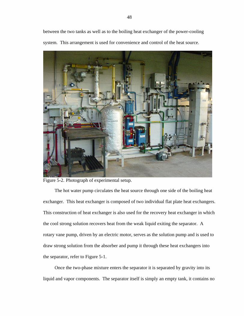
Instrument Settings ...................................................................................................127 Data Acquisition System ...................................................................................127 Gas Chromatograph...........................................................................................127
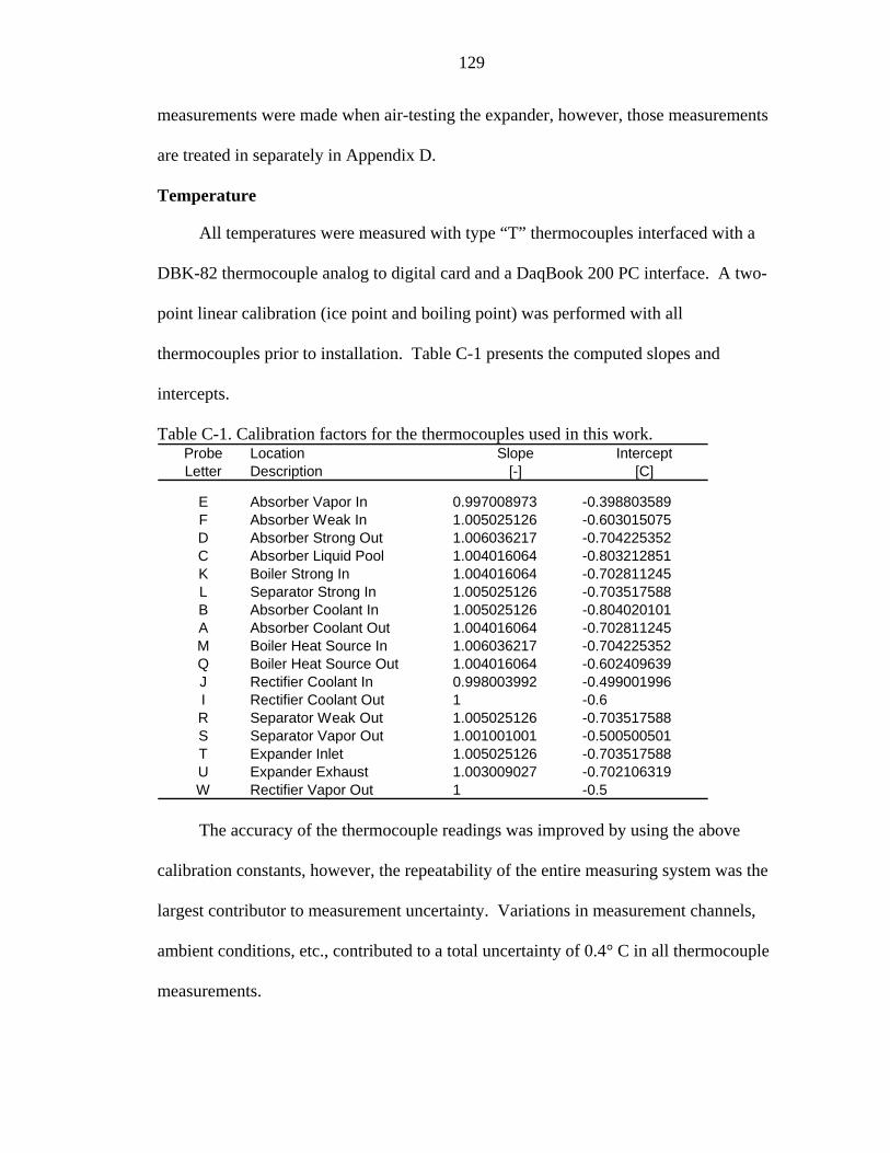
Uncertainty of Direct Measurements........................................................................128 Temperature.......................................................................................................129 Pressure..............................................................................................................130 Volume Flow Rate.............................................................................................130 Concentration ....................................................................................................131 Shaft Speed........................................................................................................132
Uncertainty of Derived Measurements.....................................................................133 Vapor Concentration .........................................................................................133 Mass Flow Rates................................................................................................134 Power Output.....................................................................................................135 Expander Efficiency ..........................................................................................135
Table page 3-1 Flow identification for the configuration of Figure 3-1. ..........................................18
4-1 Fluid properties for a typical ammonia-water concentration and other power cycle fluids for isentropic expansion from saturated conditions at 100° C to condensation/absorbtion at 35° C............................................................................34
4-2 Single stage specific speed calculations versus nominal work output and shaft speed. .......................................................................................................................36
4-3 Approximate specific speed and specific diameter ranges for efficient (>60%) single stage expander types [49, 50]. ......................................................................37
4-4 Reported turbine operating parameters and efficiencies for three systems using an ammonia-water working fluid [54-56]. ....................................................................38
4-5 Estimated operating data for the three turbine stages of a Kalina-based bottoming cycle [53]. .................................................................................................................39
4-6 Reported efficiencies of scroll expanders [18, 20, 62, 63].......................................40
6-1 Measured decrease of absorption pressure with basic solution concentration.........61
6-2 Measured data indicating effects of absorption temperature....................................63
6-3 Averaged values for rectifier operation....................................................................63
6-4 Values for rectifier operation highlighting penalty to work production. .................64
6-5 Averaged conditions for the testing of Figure 6-4. ..................................................66
7-1 Typical operating characteristics for cooling and work optimized cycles. ..............75
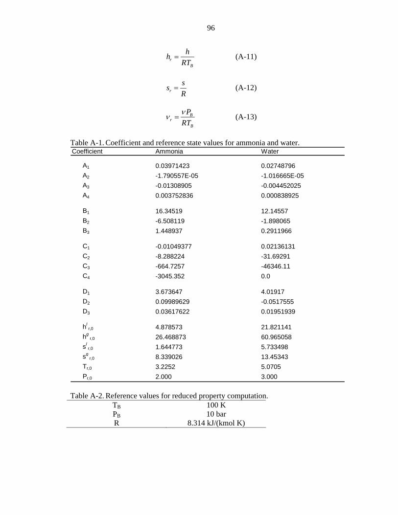
A-1 Coefficient and reference state values for ammonia and water................................96
A-2 Reference values for reduced property computation................................................96
A-3 Coefficient values used to compute excess properties. ............................................98
ix
A-4 Coefficient values for the determination of mixture bubble and dew point temperatures. ..........................................................................................................100
B-1 Flow identification for the configuration of Figure B-1. .......................................107
C-1 Calibration factors for the thermocouples used in this work..................................129
2-1 Schematic of the power-cooling cycle. ....................................................................11
2-2 Ammonia-water phase equilibrium diagram highlighting the source of cooling temperatures. ............................................................................................................12
3-1 Power-cooling schematic used for modeling. ..........................................................19
3-2 Conceptual relationship between the factors affected by boiling pressure. .............21
3-3 Output parameter variation as a function of boiling pressure. .................................22
3-4 Variation of output parameters as a function of basic solution concentration. ........23
3-5 Effect of boiler exit temperature on output parameter profiles. ...............................24
3-6 Computed effect of vapor concentration and inlet temperature on expander exhaust temperature...............................................................................................................26
3-7 Computed effect of expander efficiency and inlet temperature on expander exhaust temperature...............................................................................................................26
3-8 Beneficial effect on expander exhaust temperature as a function of increasing rectification…...........................................................................................................28
3-9 Effect of rectification and rectifier efficiency on work production..........................29
5-1 Schematic of experimental setup..............................................................................47
5-2 Photograph of experimental setup............................................................................48
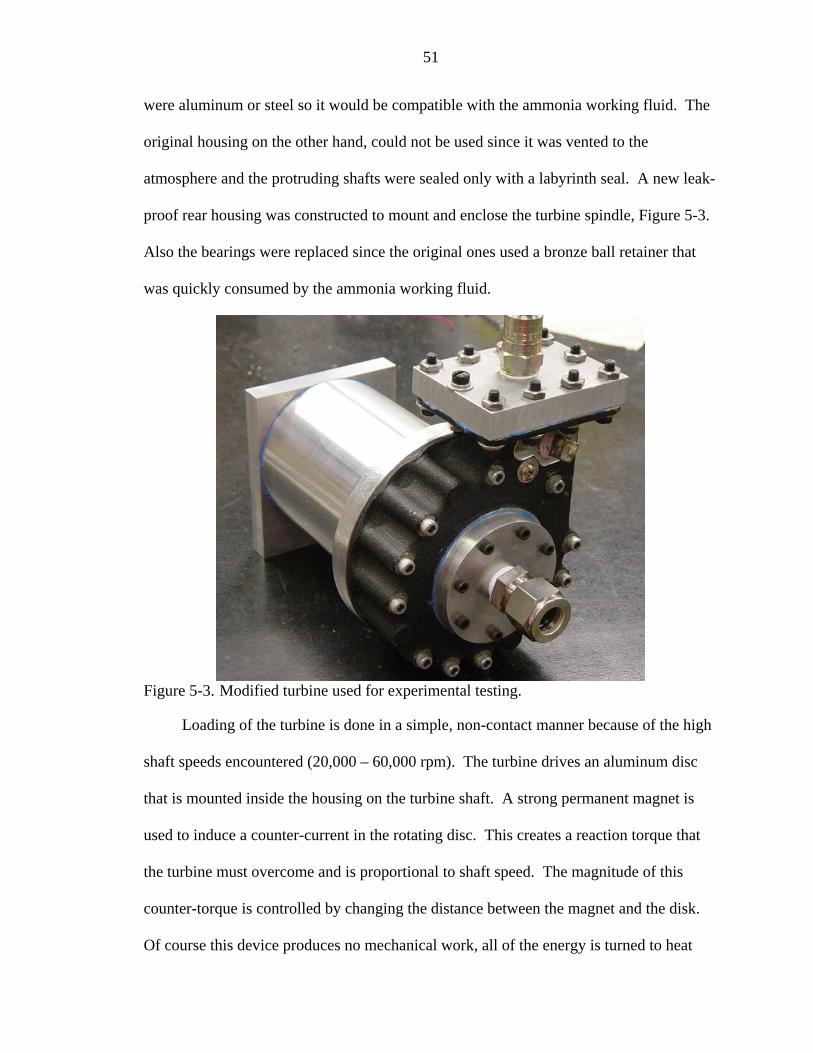
5-3 Modified turbine used for experimental testing. ......................................................51
5-4 Original and modified absorber configurations. ......................................................53
6-1 Measured effect of pressure variation on vapor quantity and concentration. ..........60
xi
6-2 Measured effect of basic solution concentration on vapor production. ...................61
6-3 Measured change in vapor flow rate (relative to basic solution flow) due primarily to changes in boiling temperature. ...........................................................................62
6-4 Experimental measurement of the expansion of vapor to temperatures below those at which absorption-condensation is taking place....................................................65
6-5 Expected equilibrium exhaust qualities for conditions similar to those of the experimental study. ..................................................................................................68
6-6 Temperature-enthalpy diagram covering the phase change of pure ammonia and a high concentration ammonia-water mixture. ...........................................................69
6-7 Comparison between the measured no-load power consumption of operation with compressed air and ammonia-water. ........................................................................70
7-1 Maximum effective COP values where the work component is the amount of work lost due to operation with rectification vs. equivalent conditions with no rectification...............................................................................................................74
7-2 Maximum overall effective COP values as defined by Equation 7-2. .....................76
7-3 Corresponding exhaust temperatures for the optimum conditions presented in Figure 7-2. ................................................................................................................76
7-4 Design point map showing the relative sensitivity of overall effective COP to vapor mass flow fraction and exhaust temperature. ...........................................................78
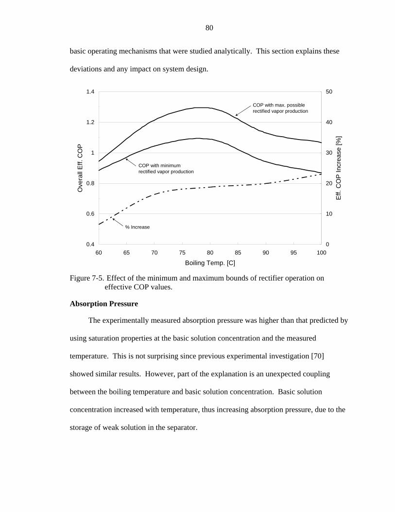
7-5 Effect of the minimum and maximum bounds of rectifier operation on effective COP values. ..............................................................................................................80
7-6 Computed effect of weak solution storage on basic solution concentration. ...........82
7-7 Computed absorption pressures taking into account the changes of basic solution concentration compared with measured absorber pressures. ...................................83
7-8 Measured drop in boiling pressure due to rectifier operation. .................................84
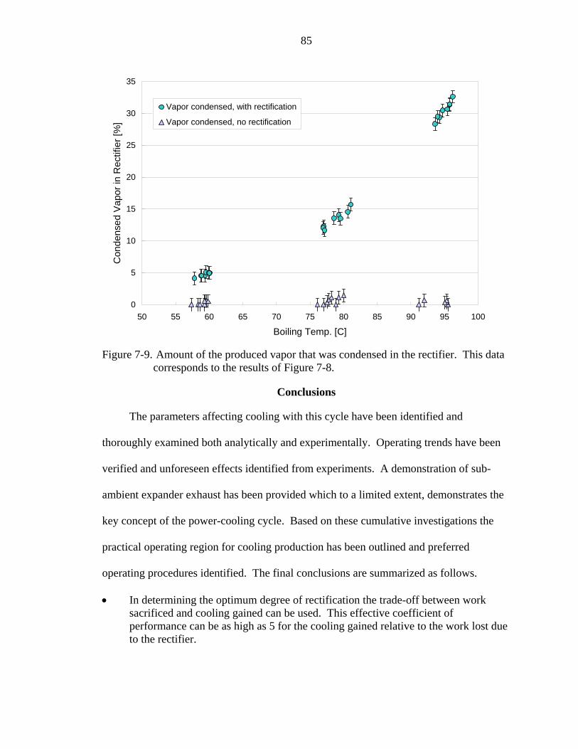
7-9 Amount of the produced vapor that was condensed in the rectifier. This data corresponds to the results of Figure 7-8. ..................................................................85
B-1 Schematic used for the theoretical modeling. ........................................................107
C-1 View of the assembled rear housing. .....................................................................138
C-2 Exploded view of the rear housing assembly.........................................................139
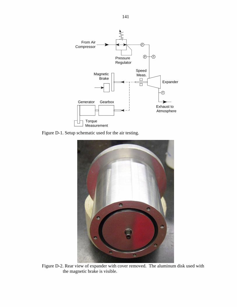
D-1 Setup schematic used for the air testing. ................................................................141
xii
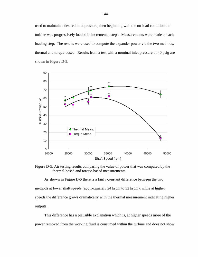
D-2 Rear view of expander with cover removed...........................................................141
D-3 Photograph of generator loading arrangement. ......................................................142
D-4 Photograph of gearbox mounted on expander spindle. ..........................................143
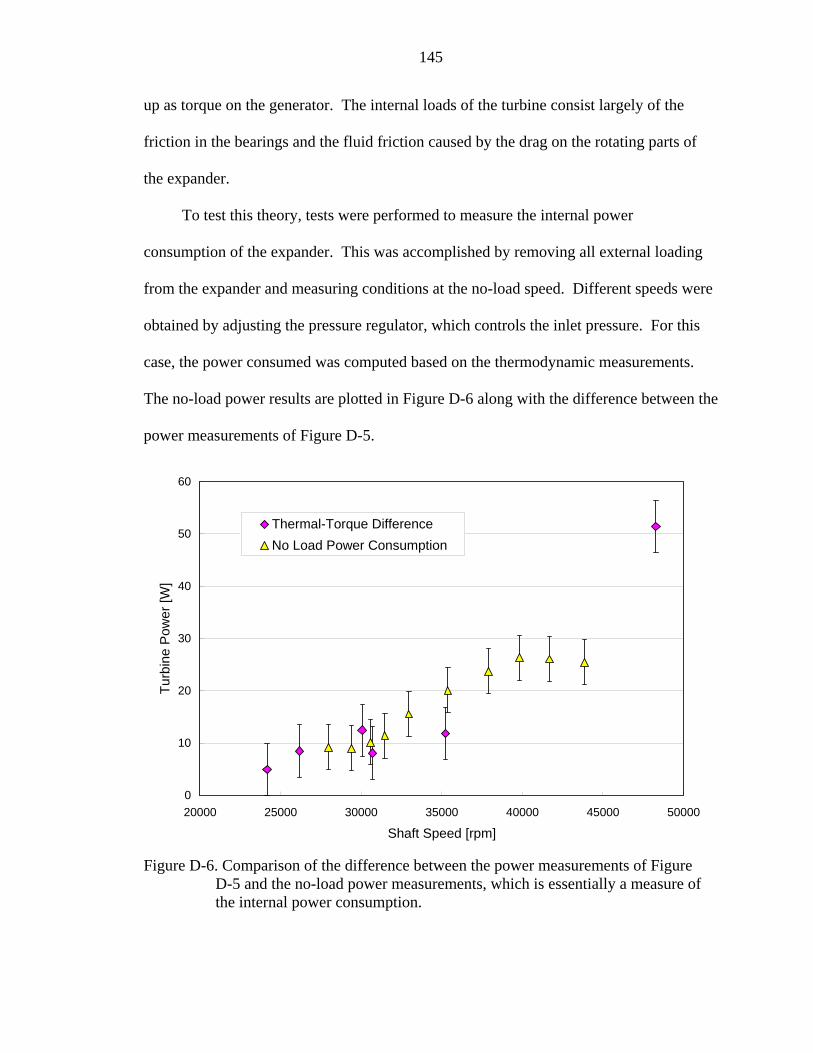
D-5 Air testing results comparing the value of power that was computed by the thermal-based and torque-based measurements. .................................................................144
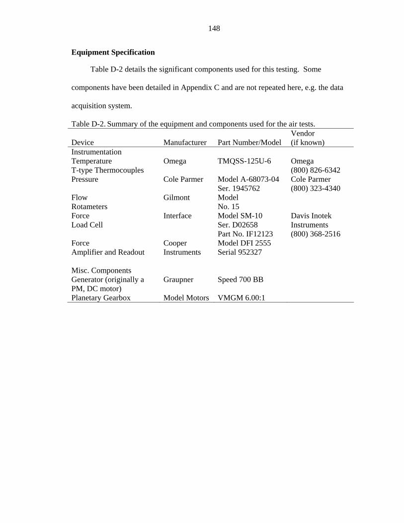
D-6 Comparison of the difference between the power measurements of Figure D-5 and the no-load power measurements, ….....................................................................145
xiii
NOMENCLATURE
A area under mV-time curve COP coefficient of performance cp constant pressure specific heat D diameter, [m] dspec specific diameter parameter G Gibbs free energy h enthalpy m& , m mass flow rate, [kg/s] nspec specific speed parameter ORC organic Rankine cycle OTEC ocean thermal energy conversion P pressure, [MPa] Pr pressure ratio q heat transfer, [kJ/kg] Q heat transfer, [W], volume flow Qact actual volume flow rate Qexit expander exit volume flow rate, [m3/s] Qind indicated volume flow rate R universal gas constant Rc/w ratio of cooling to work
xiv
s entropy T temperature, [°C] W work output/input, [W] x ammonia mass concentration [kg/kg], mixture quality y fraction of working fluid that is stored in separator ∆hideal isentropic enthalpy change Subscripts
1stLaw first law formulation a ammonia component properties absorber absorber parameter actual actual parameter values B reference properties basic new new basic solution parameter with storage basic org original basic solution parameter before storage boiler boiler parameter bubble saturated liquid properties cal calibration parameter values cool cooling heat exchanger parameter crit-water water critical point properties dew saturated vapor properties effective effective value formulation exit expander exit condition expander expander parameter
xv
float float properties inlet expander inlet condition m mixture properties no rect conditions with no rectifier operation overall overall comparison, with cooling production and work optimized pump pump parameter r reduced properties recovery recovery heat exchanger properties s strong solution, isentropic end state superheat superheater parameter v vapor vr rectified vapor w weak solution, water component properties wb weak solution from boiler w/cool conditions with cooling production wr weak solution from rectifier with rect conditions with rectifier in operation workopt conditions optimized for work output 0 reference state properties Superscripts
E excess properties g gas phase properties l liquid phase properties mix parameters of mixing
xvi
Greek
η efficiency ν specific volume ρ density ω angular velocity, [rad/s]
xvii
Abstract of Dissertation Presented to the Graduate School of the University of Florida in Partial Fulfillment of the Requirements for the Degree of Doctor of Philosophy
STUDY OF COOLING PRODUCTION WITH A COMBINED POWER AND COOLING THERMODYNAMIC CYCLE
By
Christopher Martin
December 2004
Chair: D. Y. Goswami Major Department: Mechanical and Aerospace Engineering
This work is an investigation of a novel concept to produce power and cooling with
the energy contained in low-temperature (< 200° C), thermal resources. These resources
can be obtained from non-concentrating solar thermal energy, low-grade geothermal
resources, and a near infinite variety of waste heat sources. The concept under
investigation uses thermal energy in a low-temperature boiler to partially boil an
ammonia-water working fluid mixture. This produces an ammonia rich vapor that drives
an expander. The expander’s output is mechanical power; however, under certain
operating conditions its exhaust can be cold enough to use for cooling. This possibility is
the focus of the present study.
An analytical study is presented which identifies expander efficiency, expander
inlet conditions, and exhaust pressure as the factors determining exhaust temperature.
Estimated expander efficiencies are based on a consideration of the operating conditions
and a review of current technology. Preferred inlet conditions are identified; however,
xviii
they are linked to the overall operation of the cycle, as is absorption pressure. An optimal
balance between vapor generation and expander exhaust temperature is found for cooling
production.
Purifying the vapor is shown to enhance cooling production, but it penalizes work
output. A new coefficient of performance is defined as the ratio of the cooling gained to
the work output lost and is used to determine the optimal purification. Additionally,
another performance coefficient is defined and used to judge the overall value of cooling
produced.
An experimental study is presented that verifies the predicted trends. Furthermore,
a measurement of sub-ambient exhaust temperatures is provided that demonstrates the
key concept of this cycle. It is concluded that with improved expander performance,
practical power and cooling production can be achieved with this concept. Deviations
between measured and simulated performance are discussed as they relate to improving
future modeling and system design efforts.
1
CHAPTER 1 INTRODUCTION
The conversion of thermal energy into mechanical work is a fundamental task of
mechanical engineering. Performing it cleanly, cheaply and efficiently all influence the
eventual conversion scheme. Rankine-based cycles enjoy widespread usage and are
particularly suited for low resource temperatures since their operation can approximate
that of a Carnot engine.
Many adaptations and modifications have been made to the basic Rankine cycle in
order to extract the most energy from heat sources such as geothermal wells, solar
thermal energy, and waste heat streams. A relatively recent cycle has been proposed in
which thermal energy is used to produce work and to generate a sub-ambient temperature
stream that is suitable for cooling applications [1]. It has been the focus of theoretical
and experimental investigation [2-5]; however, until this work, there has not been a
complete, experimental implementation of this power-cooling cycle. Therefore, this
study is an investigation, both theoretical and experimental, into the distinguishing
feature of this concept, which is cooling production.
The cycle is a combination of Rankine power production and absorption
refrigeration cycles, and is unique in power production cycles because it exploits the
temperature drop across an expander to the point of being able to obtain useful cooling.
Optimization of system parameters, working fluid selection, and preliminary
experimentation with the cycle have been performed [2-5]. What this work provides is
an experimental proof-of-concept that demonstrates the key feature of this cycle. Also
2
included is a discussion of the parameters affecting cooling production and a method to
quantify its production.
Certainly this work advances the development of this power-cooling cycle, but
more importantly, research in the field of heat recovery is an active step in moving
society toward a sustainable energy policy. This concept belongs to the broader class of
low temperature, Rankine based cycles which have been shown to be one of the most
effective means for utilizing low temperature resources. They have been applied to the
production of mechanical power using heat from solar, geothermal, and waste heat from
topping power cycles and industrial processes. Despite their wide range of possible
applications, these systems have found limited success in practice. It is hoped that this
work will aid any resurgence in today’s energy market.
Motivation
The wide-ranging motivation for this work comes from the possible applications
for this category of low temperature, Rankine based cycles. Being simply a heat engine
with the potential for good second law efficiencies, the possible recovery applications are
limited only by the economics of the situation. In the future, the economics may be more
favorable to devices that can produce power without additional resource consumption.
When considering the future of world electricity production, the only apparent
certainty is that generation will be done by more diverse means than it is currently [6]. It
appears that the paradigm of a few, large, centralized power producers is becoming more
conducive to adding more, smaller, distributed generators. There are many reasons for
this; key among them are to increase the reliability of the electrical system by promoting
diversity, provide cleaner energy by incorporating more renewables, and simply to
increase capacity to meet additional demand.
3
The distributed generation trend will open opportunities in two key ways. First, by
adding smaller distributed generators, the mechanics of connecting to the grid will no
longer be prohibitively complex, but will become more routine. Second, with on-site
generation the opportunities to recover and use waste heat resources will make economic
sense. In fact, the U. S. Department of Energy expects the utilization of waste heat alone
to provide a significant source of pollution-free energy in the coming decades [7].
Viewed in this way, the use of a low-temperature power cycle is one of the many
possible distributed technologies that could connect to the grid or be used to recover
thermal resources. They can be used on a small scale to convert renewable energy
sources, use conventional fuels efficiently, or conserve energy by recovering waste heat
from energy-intensive processes, Figure 1-1. Ultimately they would have positive
impacts on overall energy conversion efficiency and could be used to incorporate
renewable energy sources.
AdaptableORC
ConventionalFuel
ToppingCycle
SolarThermal
Waste Heat
Combustion
Power
Figure 1-1. Ideas for using an ORC to incorporate a renewable element into distributed power generation. Efficient use of multiple energy sources would require a highly adaptable heat engine and, of course, any configuration would have to be economically viable.
4
Power-Cooling Concept
This work is not directly aimed at reducing the cost of this technology. Rather it is
directed at improving the underlying science to make it more versatile and thus more
attractive for implementation. Mechanical power is one useful form of energy, the
generation of low temperatures for cooling or refrigeration is another. The cycle under
study in this work was intended to explore the feasibility of using thermal resources to
simultaneously produce these two useful outputs.
Put simply, the configuration of this power-cooling cycle allows the vapor passing
through the turbine to be expanded to below ambient temperatures. Cooling can then be
obtained by sensible heating of the turbine exhaust. A more detailed explanation of this
process follows in Chapter 2, but here it suffices to say that the use of a working fluid
mixture, ammonia-water, is the key to this process. Just as in conventional aqua-
ammonia absorption cooling, absorption-condensation is also used here to regenerate the
working fluid. This eliminates the expansion temperature restriction which is in place
when pure condensation is used.
The power-cooling cycle has the obvious advantage of two useful outputs, but it
has other attributes that make it an attractive energy conversion option. The first of these
characteristics is that the cycle uses a binary working fluid that has a variable boiling
temperature at constant pressure. This avoids heat exchange “pinch point” problems that
pure component working fluids experience due to their constant phase change
temperature at constant pressure. In addition, turbine designs for ammonia-water are
reasonably sized for large power outputs when compared to the more traditional organic
working fluid choices.
5
Problem Definition
The distinguishing feature of this cycle, compared to other power cycles and even
those in the developing class of combined power and cooling cycles, is the method in
which cooling is produced. In other power cycles the working fluid is regenerated by
pure condensation, rather than absorption-condensation which is used here; this limits the
minimum turbine exhaust temperature to roughly the temperature at which condensation
is taking place. When considering other combined power-cooling cycles, cooling is
typically produced in the same manner as a conventional absorption system, that is,
condensation and throttling of the refrigerant. Here in this cycle, vapor is expanded
through a turbine to produce power and because of the advantage of absorption-
condensation, it can be expanded to sub-ambient temperatures.
While the method of cooling production is the key feature of this cycle, until this
work it has not been experimentally investigated. What has been experimentally
investigated are the underlying boiling and absorptions processes [4]. For those
experiments a turbine was not implemented; its performance was simulated with an
expansion valve and a heat exchanger. Coupled with the lack of experimentation, the
question of implementing cooling production with this concept has not been treated in
any depth.
Discussion of the possible uses of this cycle have suggested the utilization of solar
thermal, geothermal, or waste heat resources. However, a proper use for the potential
cooling output has not been put forward, possibly because the specific nature of an
application will be determined by the characteristics of cooling production. There has not
been a thorough discussion of the trends of cooling production.
6
Research Objectives
In response to the deficits mentioned in the previous section, the objectives of this
work are to experimentally implement a turbine for power production and identify the
factors important for cooling production and investigate them analytically and
experimentally. Analytically, the study will identify the conditions favorable for cooling
production, estimate performance using available expander technologies, and quantify
cooling production in terms of energy consumption. In addition, this work will
experimentally investigate the concepts key for cooling production and document design
and operating experience for use with future modeling or implementation efforts.
7
CHAPTER 2 BACKGROUND AND REVIEW
The purpose of this chapter is to introduce the concept of this cycle in the context
of both low temperature thermodynamic power cycles and conventional cooling cycles.
In addition, to accurately provide the context for this work, a review of previous effort
into this concept is presented.
As an overview, the power-cooling cycle is best described as a compromise
between a conventional aqua-ammonia absorption system and a Kalina-type power
generation cycle. It is a continuation of the evolution of binary mixture Rankine cycles
but makes use of the cooling effect possible due to the working fluid concentration
change. As for previous work on this cycle, numerous theoretical studies have been
produced and initial experimentation has begun. From a review of that work, this study
is shown to be the first experimental confirmation of the power-cooling cycle’s key
concept and to provide initial consideration for system operation.
Background
The thermodynamic conversion of low temperature resources into mechanical
power traces its roots to at least the beginning of the industrial revolution. Utilizing solar
thermal energy to pump water was the impetus and this work continued haphazardly until
the early decades of the twentieth century when it was interrupted by World War I and
the discovery of a new resource, oil and gas [8]. Modern research into low temperature
power conversion surfaced again when the panacea of cheap coal power was beginning to
break down and energy alternatives were sought in the decades following World War II.
8
The application was utilizing liquid-producing, geothermal fields where flash boiling is
not suitable [9]. Additional interest came during the 1970’s oil crisis in using these low
temperature engines for solar thermal energy and heat recovery applications. The
common description for these systems is organic Rankine cycle (ORC) engines, because
many of the working fluids are organic hydrocarbons or refrigerants.
ORC Development
Intense research of non-geothermal ORC use took place in this country during the
early 1970’s through the early 1980’s. ORC heat engines were reconsidered for utilizing
solar resources and conserving other resources by recovering energy from waste heat.
Seemingly no application was overlooked as a few innovative examples illustrate. In one
an ORC was integrated with a large truck engine to recover heat from the exhaust and
save on fuel costs [10] and in another application the idea of replacing the automobile
internal combustion engine with an ORC system was explored [11].
Mechanical cooling systems were one of the more productive research areas that
dealt with the conversion of solar thermal energy. A significant amount of the published
literature regarding ORC conversion of solar thermal energy comes from this and related
work [12]. The concept started as an alternative to solar-driven, absorption, air-
conditioning cycles which have a limited coefficient of performance. Essentially,
mechanical work produced by a solar-driven ORC would be used to drive vapor-
compression air conditioning equipment, with the potential of a higher COP than
absorption equipment [12]. These projects produced many successful prototype units
( e.g. [13] ) and led to a feeling of technical maturity for the low-temperature, small-
scale, conversion of solar thermal energy [14]. As for ORC technology today, it has
found some niche successes in geothermal utilization, biomass utilization, some industrial
9
heat recovery, and cathodic protection of pipelines, as judged by a few manufacturer’s
portfolios.
More recent research in the area has largely taken place internationally ( e.g. [15-
18] ), with much interest being placed on expander implementation. Two approaches
have been noted: one is to develop and design systems around high-speed
turbomachinery with a shaft integral generator and circulation pump [19], thus reducing
costs by simpler design, and the other, more recent idea is to adapt mass-produced
(cheap) displacement compressors for use as reasonably efficient expanders [18, 20, 21].
Ammonia-Water Cycles
While much of the related material on ORC systems is intended for small scale
application or implementation (especially solar-driven units), the lineage that the power-
cooling cycle is derived from was initially intended for utility-scale bottoming cycle duty.
The first study of an absorption based power cycle was performed by Maloney and
Robertson [22] who concluded no significant advantage to the configuration. Several
decades later, Kalina [23] reintroduced the idea of an ammonia-water power cycle as a
superior bottoming cycle option over steam Rankine cycles. Some independent studies
have been performed [24, 25] that concede some advantage of the Kalina cycle under
certain conditions.
The key advantage of the ammonia-water working fluid is its boiling temperature
glide, which allows a better thermal match with sensible heat sources and reduces heat
transfer related irreversibilities. This same advantage, however, could be a problem
during the condensation phase of the cycle in which the condensation temperature glide
could cause a thermal mismatch with the heat rejection fluid and an increase in heat
transfer irreversibility. The solution employed is to vary the concentration of the working
10
fluid so that the fluid passing through the turbine is of different composition than that
being condensed in the condenser. In fact, by taking advantage of the chemical affinity
of ammonia and water, the condensation process can be replaced by absorption-
condensation.
Investigation of these power cycle configurations has become a new specialty in
engineering thermodynamics, and the power-cooling cycle of this work is a product of
this research area. As a result of this diversified interest, ammonia-water based power
cycles have been proposed for solar utilization, geothermal, ocean thermal energy
conversion, and other forms of heat recovery.
Power-Cooling Concept
While it was the interest brought about by Kalina’s proposal that led to the
introduction of the power-cooling cycle, it is somewhat ironic that the original suggestion
for its implementation is more similar to the original Maloney-Robertson implementation
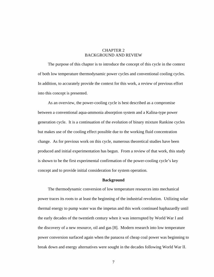
[1, 2]. Figure 2-1 is a schematic of the power-cooling cycle. Aside from the operating
parameters, the key difference between the cycle of Figure 2-1 and the Maloney-
Robertson cycle is the addition of a vapor rectifier following the boiler.
Referring to Figure 2-1, basic solution fluid is drawn from the absorber and
pumped to high pressure via the solution pump. Before entering the boiler, the basic
solution recovers heat from the returning weak solution in the recovery heat exchanger.
In the boiler, the basic solution is partially boiled to produce a two-phase mixture; a
liquid, which is relatively weak in ammonia, and a vapor with a high concentration of
ammonia. This two-phase mixture is separated and the weak liquid is throttled back to
the absorber. The vapor’s ammonia concentration is increased by cooling and condensate
separation in the rectifier. Heat can be added in the superheater as the vapor proceeds to
11
the expander, where energy is extracted from the high-pressure vapor as it is throttled to
the system low-pressure. The vapor rejoins the weak liquid in the absorber where, with
heat rejection, the basic solution is regenerated.
Rectifier
Boiler
Solution Pump
Heat Out
RefrigerationHeat Exchanger
Throttle
Recovery HeatExchanger
Absorber
Superheater
Expander
Heat In
Figure 2-1. Schematic of the power-cooling cycle.
In this configuration, the vapor temperature exiting the expander can be
significantly below ambient conditions and cooling can be obtained by sensibly heating
the expander exhaust. The temperature drop possible across the expander is due to the
fact that the working fluid is a binary mixture, and at constant pressure the condensing
temperature of an ammonia rich vapor can be below the saturation temperature for a
lower concentration liquid. This is best illustrated with a binary mixture, phase
equilibrium diagram, as shown in Figure 2-2. The low concentration saturated liquid
12
state represents the basic solution exiting the absorber, while the high concentration
vapor is typical of the expander exhaust conditions. This shows how it is possible for the
vapor to be expanded to a temperature below that at which absorption is taking place.
According to the equilibrium diagram, to maximize this temperature difference the basic
solution should be low in ammonia concentration and the vapor should be high. Also,
partial condensation of the expander exhaust would cause an additional decrease in vapor
temperature. This is entirely possible since ammonia becomes saturated upon expansion.
-20
0
20
40
60
80
100
120
0 0.1 0.2 0.3 0.4 0.5 0.6 0.7 0.8 0.9 1
Ammonia Mass Fraction
Tem
pera
ture
[C]
Pressure = 0.203 MPaVapor
Liquid
Two-Phase
Basic solutionin absorber
Expander exhaust
Figure 2-2. Ammonia-water phase equilibrium diagram highlighting the source of
cooling temperatures.
Prior Work
Since the proposal of the idea by Goswami a theoretical and experimental
investigation has been under way by a group at the University of Florida. Initial
investigations were performed theoretically and they focused on procuring reliable
13
property data for the ammonia-water mixture [26] and identifying operating trends [27,
28]. Later studies concluded that the cycle could be optimized for work or cooling
outputs and even for efficiency. Optimization studies began to appear, optimizing on the
basis of various efficiency definitions, minimum cooling temperature, working fluid
combination, and system configuration. Also, an experimental study was described by
Tamm and Goswami [4] which generally verified the expected boiling and absorption
processes.
Goswami and Xu [27] presented the first theoretical analysis of the power-cooling
cycle. Turbine inlet temperatures of 400 – 500 K were considered along with absorption
temperatures of 280 – 320 K. Cooling production suffered with increased turbine inlet
and absorption temperatures, and benefited with increased boiler pressure. Many of the
operating trends of importance in this work were introduced here.
Optimization studies began to appear following this work, which identified the
balance of effects that dictate cycle operation. Lu and Goswami [2] optimized the ideal
cycle conditions using various objectives, work output, cooling output, first and second
law efficiencies. All operating parameters, efficiencies, power/cooling output, etc., were
found to decrease with increasing heat rejection temperatures. At high heat source
temperatures, 440 K, no cooling was possible at conditions optimized for second law
efficiency. A contrast between work optimized and cooling optimized cases was
provided. Important differences in the cooling optimized case versus the work optimized
one were higher vapor concentration, lower turbine inlet temperature, low vaporization
fraction (16.5 % vs. 91.2 %), and a lower basic solution concentration. Minimum cooling
14
temperatures were also optimized [29], and a minimum turbine exhaust temperature of
205 K was identified under the assumptions considered.
The question of appropriate efficiency expressions for the cycle was tackled by
Vijayaraghavan and Goswami [30]. The conditions obtained from an optimization study
were found to be heavily influenced by the weight given to the cooling output. Some
expressions simply added the outputs of power and cooling, which gives an overestimate
of system performance, or cooling was weighted by an ideal COP value computed for
equivalent temperature limits, which tends to underestimate the value of cooling. They
[30] introduced a satisfactory second law efficiency definition based upon ideal Lorenz
cycle performance which accounts for sensible heat addition and rejection behavior.
However, they concede that ultimately the value of work and cooling will be decided by
the end application [30].
Both first and second law efficiency analyses were performed for the cycle [31,
32]. A second law efficiency of 65.8 % was determined, using the definition of [30], for
the idealized model considered. The largest source of irreversibility was found to be the
absorber at all conditions considered; while at higher heat source temperatures the
rectifier also contributed significantly.
Less-than-ideal modeling began with Tamm et al. [33, 34], in preparation for the
initial experimental studies [4]. The largest deviation from idealized simulations was due
to the non-isentropic performance of the turbine. This relates well to the findings of Badr
et al. [35], who identified the expander isentropic efficiency as the single-most influential
factor affecting overall ORC engine performance. Initial experimentation was reported
[36]; however, turbine operation was simulated by an expansion valve and a heat
15
exchanger. General boiling condition trends were demonstrated, for example vapor mass
flow fraction, vapor concentration, and boiler heat transfer. Vapor production was less
than expected and improvements to the setup were identified and implemented.
Performance of the new configuration, still having a simulated turbine, was also reported
[4]. Vapor production and absorption processes were shown to work experimentally,
however still with some deviations.
An independent study of the power-cooling concept has been provided by Vidal et
al. [37], who also noted the significant impact of non-ideal turbine performance on
cooling production. Vidal et al. also reported poor cooling production at higher ambient
conditions.
Other Power-Cooling Concepts
The development of the power-cooling cycle under investigation in this work has
been presented as it relates to other power production cycles. However, there is now a
small class of combined power and cooling cycles, especially since the proposal by
Goswami [1]. Differentiation of this concept from others in the literature is now
presented.
Oliveira et al. [38] presented experimental performance of an ORC-based,
combined power-cooling system which used an ejector placed in-parallel to the turbine
for cooling production. Ejector cooling has been an academic topic for solar thermal-
powered cooling, for example [39, 40]. The implementation and operation of an ejector
cooling system is quite simple and rugged; however, its COP tends to be low and in this
combined case it siphons away high pressure vapor directly from the turbine that could
have been used to produce power.
16
Considering integrated, ammonia-water cycles, Erickson et al. [41] present the
most intuitive. The proposal is essentially an absorption cycle, with advanced thermal
coupling between the absorber and generator, with a turbine placed in-parallel to the
condenser and evaporator. So vapor is produced and, depending on the outputs desired,
split between expansion in a turbine or condensation and throttling in the refrigeration
path. Integration comes from the common components, for example the absorber,
generator, and feed pumps. However, the mechanism of cooling is the same as that for
an aqua-ammonia absorption system. The very pure ammonia vapor is condensed at high
pressure and throttled to the absorption pressure where flash boiling and evaporation take
place.
The concept of parallel paths for power and refrigeration production has been
incorporated with the thermal-matching concepts of a Kalina cycle by a research group at
Waseda University [42]. Unlike the proposal by Erickson et al., however, only the
working fluid is shared between the two systems. The power production and
refrigeration cycles can be driven independently, but it was found that more power could
be produced by sharing the working fluid [42]. Therefore, cooling in this case is also
produced in the same manner as with an aqua-ammonia absorption system.
A more thorough integration of power and refrigeration production has been
recently proposed by Zhang et al. [43]. In this configuration the ammonia-water basic
solution is separated into a high concentration ammonia vapor and a relatively weak
solution liquid in a device similar in operation to a distillation column. The vapor is
condensed and throttled to produce cooling while the weak solution liquid is vaporized
and superheated, then expanded in a turbine for power production. The streams are then
17
cooled and rejoined in an absorber. The authors claim a 28% increase in exergy
efficiency of this arrangement over separate steam Rankine and aqua-ammonia
absorption systems [43]. As with the other concepts, cooling is produced the same way
as with a aqua-ammonia absorption system.
Conclusion
As compared to other power and cooling concepts, the distinguishing feature of this
cycle is the method in which cooling is produced. Its configuration is most similar to that
of an aqua-ammonia absorption system; however, instead of using condensation and
throttling for cooling production an expander is used to extract energy from the vapor--to
the point that cooling can be obtained from the exhaust. As compared to the absorption
cycle, the trade-off for work production is reduced cooling since no latent heat is
involved. The remainder of this work will discuss the opposite situation, the penalty to
power cycle operation due to combined cooling production.
18
CHAPTER 3 THEORETICAL STUDY
In this chapter a model of the system is presented and used to simulate the steady
state performance of the power-cooling cycle. With this model, a straightforward
parametric study is carried out which identifies the essential operating mechanisms
affecting cooling production. These results are used to design the experiments discussed
in Chapters 5 and 6 and again to extrapolate the data used for the final conclusions.
Model
The model used for this work is based upon the schematic of Figure 3-1 which has
subtle differences from the one in Figure 2-1 to be more representative of the
experimental system. Table 3-1 contains the identifying information for the working
fluid streams in Figure 3-1.
Table 3-1. Flow identification for the configuration of Figure 3-1. Identifier/ Subscript
Description
s Basic (strong) solution flow from absorber through boiler v Vapor flow produced from partial vaporization in boiler vr Rectified vapor passing through turbine and cooling heat exchanger w Weak (in ammonia) solution liquid returning to absorber wr Weak condensate formed in rectifier wb Weak liquid produced from partial vaporization in boiler
For the purposes intended, it was adequate to use first order approximations for
each component, conservation of mass and energy, so detailed component modeling was
not included. The complete formulations that were used in the computations, as well as
the subroutines themselves, can be found in Appendix B; however, the key points are
summarized as follows.
19
HeatSource
Recovery HeatExchanger
Throttle
Boiler
Absorber Coolant
Separator
Coolant Rectifier
Expander
vr
SolutionPump
v
wb
w
wr
s
Superheater
HeatSource
Cooling HeatExchanger
CooledFluid
Figure 3-1. Power-cooling schematic used for modeling.
• The boiling conditions are completely specified, i.e. boiling temperature, pressure, and basic solution concentration are provided as inputs. This means that the quality at boiler exit is allowed to be determined in accordance.
• The system low pressure is dictated by the basic solution concentration and the minimum absorption temperature, both of which are specified.
• Isentropic efficiencies are assumed for the pump and expander while effectiveness values are used for heat exchangers.
• The degree of rectification is determined by specifying the rectifier exit temperature. Similarly, the superheater exit temperature is also specified.
In addition to the specifications above, which are needed to determine the steady
state conditions, the following stipulations were enforced to avoid computational
problems and/or make the scenarios closer to reality.
• The minimum absorption temperature considered was 25° C with most attention given to 35° C cases.
20
• Vapor rectification was limited by either the specified rectifier exit temperature or an ammonia mass fraction of 0.999, whichever was encountered first. The minimum rectification temperature considered was 35° C.
• The minimum amount of vapor leaving the rectifier that was allowed was 5 % of the basic solution flow rate.
• The quantity of cooling produced (if any) was calculated as the energy needed to heat the expander exhaust from the exhaust temperature to 15° C.
Thermodynamic property data for the ammonia-water working fluid is essential for
this type of modeling. The correlations used are based on those presented by Xu and
Goswami [26] which are a combination of the Gibbs free energy method for mixture
properties and empirical equations of bubble and dew point temperatures for phase
equilibrium. Details of the complete correlations and their implementation into C++ can
be found in Appendix A.
Operating Mechanisms
Early in the theoretical investigation of this cycle it was determined that the system
could be optimized for various outputs [27]. In this section, simulated data is used to
illustrate these optimums and the balance of effects that causes them. Boiling conditions
are considered first and then the effects of heat rejection conditions.
First consider the independent effects of the parameters at the heart of the power-
cooling cycle, the boiling conditions. These effects are common to all binary mixture
power cycles; however, it will be shown that they have added significance for cooling
production.
Effect of Boiling Pressure
The boiling pressure in the power cycle is regulated by the rate of vapor production
and the rate at which vapor is released through the restriction imposed by the expander.
For a binary mixture working fluid at constant temperature and having constant
21
composition boiling takes place over a range of pressures from the saturated liquid state
to the saturated vapor state. At the upper extreme boiling pressure is limited by the
corresponding saturation pressure, above which no vapor is produced. The lower
pressure extreme is bound by the system low pressure or the absorption-condensation
pressure. Depending on the conditions, the working fluid may or may not be fully
vaporized at the lower pressure extreme.
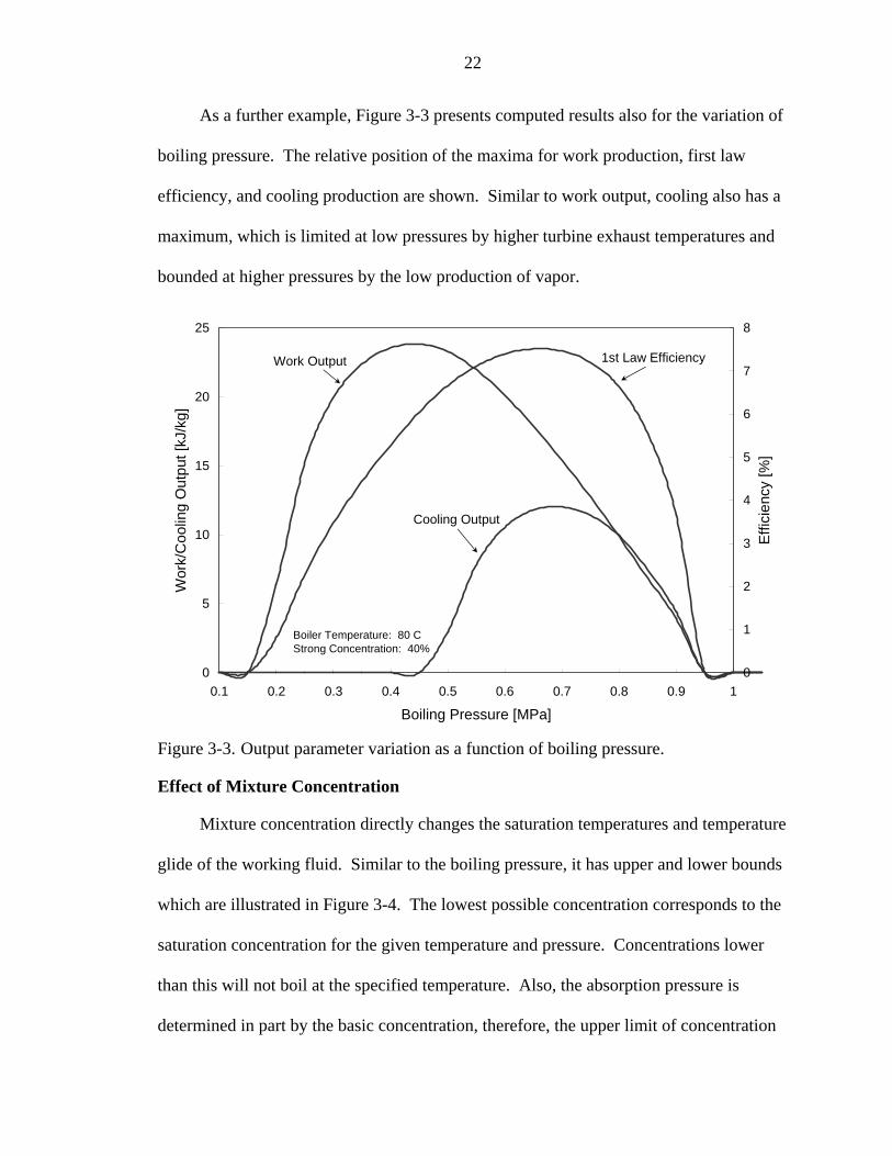
Figure 3-2 is a graphical representation of the mechanisms of variable pressure
boiling. As can be seen the mass flow rate of vapor changes inversely with pressure
ratio. Also, a quantity like the work output (assuming constant efficiency expander),
which is dependent on both the pressure ratio and amount of vapor flow, contains a
maximum within the boiling region. Work production is bounded by a unity pressure
ratio at low boiling pressure and zero vapor flow at the highest boiling pressure.
A word regarding the operation of the rectifier is appropriate here. There are many
physical setups that can be used to purify the vapor, with some being more efficient, in
terms of purified vapor flow, than others. For this work, upper and lower limits to
29
rectifier efficiency are considered. The upper bound is the theoretical maximum of
rectified vapor that can be produced as determined from a mass balance of the rectifier.
This could be implemented with a direct contact, counter-flow heat exchanger where
additional ammonia is scavenged from the counter-flowing condensate. The lower
bound, which represents the arrangement of the experimental setup and the computer
model, is the flow rate that occurs with simple cooling of the vapor and condensate
separation. No attempt to recover ammonia from the condensate is made. The effects of
this vapor-production efficiency are considered next.
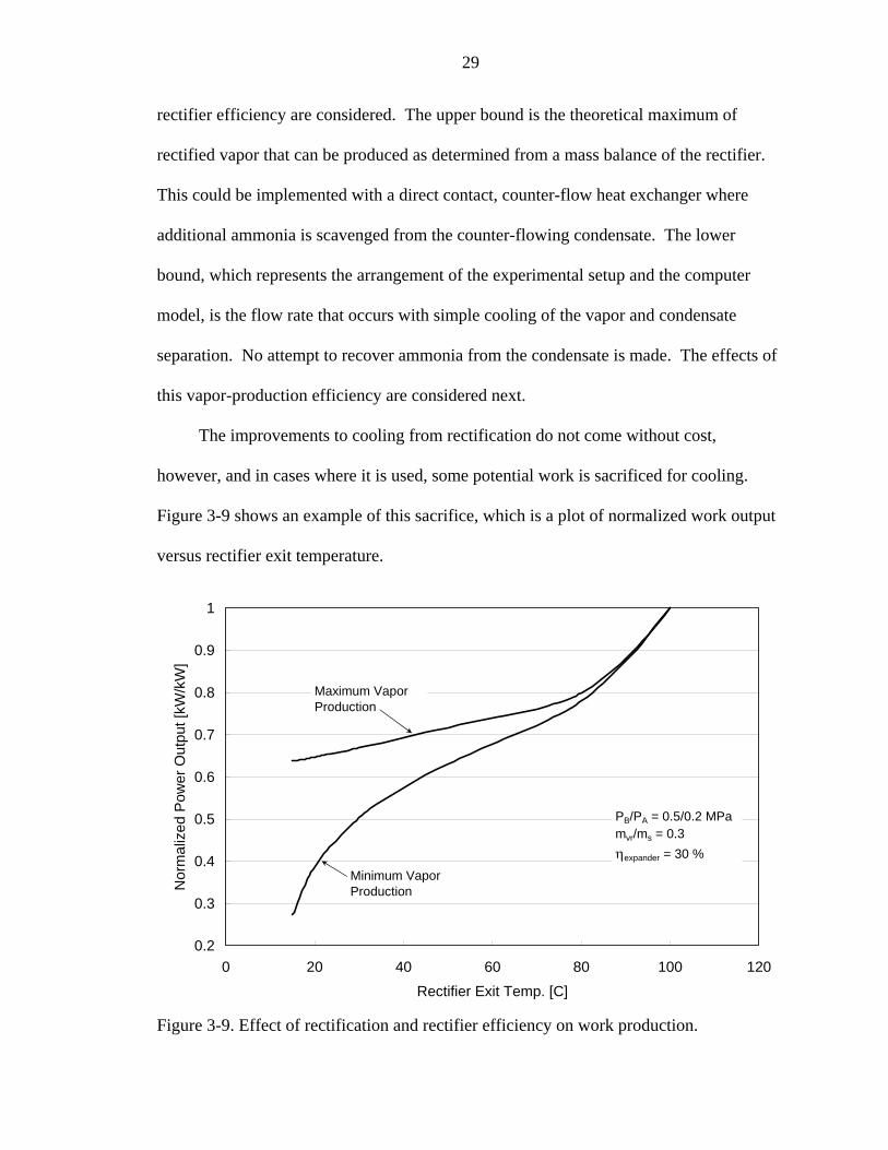
The improvements to cooling from rectification do not come without cost,
however, and in cases where it is used, some potential work is sacrificed for cooling.
Figure 3-9 shows an example of this sacrifice, which is a plot of normalized work output
versus rectifier exit temperature.
0.2
0.3
0.4
0.5
0.6
0.7
0.8
0.9
1
0 20 40 60 80 100 120Rectifier Exit Temp. [C]
Nor
mal
ized
Pow
er O
utpu
t [kW
/kW
]
Maximum VaporProduction
PB/PA = 0.5/0.2 MPamvr/ms = 0.3ηexpander = 30 %
Minimum VaporProduction
Figure 3-9. Effect of rectification and rectifier efficiency on work production.
30
The penalty to work production is caused by two factors, the decline in available
energy from cooling and the reduction in mass flow rate due to condensate formation and
separation. The combined effects of both items on normalized work output is shown in
Figure 3-9 for the upper and lower production rates for the rectifier.
As evident from Figure 3-9, at minimal amounts of rectification the difference
between rectifier performance is small. However, with increasing amounts of
rectification the difference is severe and it appears that investment in a more efficient
device may be warranted.
Performance Measures
This section describes the efficiency parameters used to evaluate the relative
performance of the power-cooling system.
Work Production
A measure of performance is needed to compare the relative efficiency of
producing work with equivalent heat source conditions and cycle configurations, and also
to identify conditions for maximum work production for a given set of heat source/sink
conditions. For this purpose, a first law efficiency formulation is adequate, Equation 3-1.
( )( )1
expander pumpstLaw
boiler superheat
W W
Q Qη
−=
+ (3-1)
Cooling Production
There is some element of personal choice involved in including cooling in an
efficiency definition. This comes from the options of converting cooling to equivalent
work terms. Other work has discussed the merits of adding work and cooling directly or
weighting cooling with a COP based on ideal cycle performance [30]. In this chapter it
has been shown that cooling and work optimums generally do not coincide, that is to
31
produce cooling some sacrifice in work has to be made. Based on this observation, an
effective COP can be defined as the ratio of the cooling produced to the work that could
have been produced, but was avoided to generate cooling. In general terms the concept
can be written as follows.
effectiveCooling GainedCOP
Work Lost= (3-2)
This term has been called the effective COP since cooling and work are only
indirectly related, in other words there is no device directly producing cooling with the
work that is given up. This definition is simply a way to determine the effectiveness, in
terms of energy, of cooling production with this cycle.
It was mentioned that some rectification is needed to produce any cooling with the
absorption temperatures considered. Recalling also that rectification diminishes work
production by the mechanisms of reduced mass flow and available energy, then some
work is inevitably lost when cooling is produced. Therefore, a more specific effective
COP can be defined based on the need for rectification, and is shown as Equation 3-3.
( )cool
effectiveno rect with rect
QCOPW W
=−
(3-3)
Conclusion
This chapter has shown the operating mechanisms affecting cycle operation. These
mechanisms determine the relative amounts of work and cooling production by affecting
the balance of vapor production, expander pressure ratio, and expander exhaust
temperature. Expander exhaust temperature is sensitive to the sensitive to the inlet vapor
conditions (pressure, temperature, and concentration), exhaust pressure, and expander
efficiency. Considering the preferred inlet conditions, the ultimate effect of the partial
32
boiling and rectification process would be to separate ammonia vapor from liquid water
rather than generate high pressure vapor for power production. The trends identified in
this chapter are used to guide the experimental study described next chapter. Also, the
implications that can be extrapolated from these trends are discussed during the
conclusion of this work.
33
CHAPTER 4 EXPANDER CONSIDERATIONS
As shown in the previous chapter, efficient operation of the expander is an obvious
requirement for cooling production within the power-cooling cycle. The purpose of this
chapter is to review the considerations for expander application in the power-cooling
cycle. An evaluation of the ammonia-water working fluid properties is given and
comparisons are made with other power cycle working fluids. These properties are
linked to design considerations for various machine types and data from the literature is
used to base estimations on the expected performance of expanders for this application.
Working Fluid Properties
In this section the thermophysical properties of the ammonia water working fluid
are considered as they relate to expander design. Ammonia is seen to behave more like
steam rather than the organic fluids that are typically used in low temperature Rankine
conversion systems. Expanders are treated in two groups, one being dynamic machines,
those that convert the fluid’s energy to velocity and create shaft power by a momentum
transfer, and the other being displacement devices, where the working fluid is confined
and allowed to expand against a moving boundary.
Table 4-1 is a comparison of fluid properties for other power cycle working fluids
as well as ammonia-water for a hypothetical, isentropic expansion. The most significant
difference between ammonia-water and the typical ORC fluids is the large isentropic
enthalpy drop of ammonia-water. This corresponds to a higher ideal jet velocity which
has an impact on dynamic turbine design. Considering steam’s characteristics, it and
34
ammonia-water are similar with respect to enthalpy drop and jet velocity. This is to be
expected because of the close molecular weights of both fluids.
Table 4-1. Fluid properties for a typical ammonia-water concentration and other power cycle fluids for isentropic expansion from saturated conditions at 100° C to condensation/absorption at 35° C. A basic solution concentration of 0.40 was assumed for the ammonia-water data.
Another way to view the losses associated with rectification is to consider the work
that was sacrificed for lower exhaust temperatures. Table 6-4 presents such information
for a couple of the cases in Table 6-3. The measured work out is the work output, per
kilogram of basic solution flow, based on experimentally measured conditions at the
point of maximum turbine efficiency. The computed work out is the estimated work that
could have been produced with the vapor not going through the rectifier but straight to
the turbine. For this calculation, the turbine’s efficiency was assumed to be the same as
the maximum measured value. The data in Table 6-4 clearly show the detrimental effect
of excessive rectification on work production.
Table 6-4. Values for rectifier operation highlighting penalty to work production. Parameter Nominal Boiling T = 60° C 95° C Measured Exhaust Temp. 25.9° C 22.3° C Max Measured Work Out 563 J/kg 1660 J/kg Computed Work w/no Rect. 612 J/kg 2600 J/kg Computed Drop in Work 7.9 % 36 %
Concept Demonstration
The realities of the experimental setup required a compromise in the testing plan.
Based on experimental measurements, the turbine, even with a single nozzle, is slightly
oversized for the experimental setup. The result is that the boiling pressure falls to a
value that is below the optimum identified in the theoretical analysis. The consequences
come in the form of reduced pressure ratios and vapor concentrations, both effects
degrade cooling production. To compensate, boiling temperatures were increased to
compromise between sufficient vapor flow rate for turbine operation and sufficient
pressure to allow for a high degree of rectification without sub-ambient condensing
temperatures. As can be concluded from the previous theoretical analysis, this incurred
65
much loss due to the rectifier, but the resulting vapor mass flow and turbine inlet pressure
was higher than could be achieved at lower temperatures. Efficiency was essentially
traded for more suitable vapor conditions.
Figure 6-4 shows the measured temperatures across the turbine in relation to the
measured absorption temperature and Table 6-5 presents the parameters for this testing.
Successive stages of rectifying and superheating enabled the production of vapor with
0.993 concentration and temperatures ranging from the vapor saturation temperature,
approximately 39° C according to Figure 6-4, up to the useful limit of the superheater.
15
18
21
24
27
30
33
35 38 41 44 47 50 53
Expander Inlet Temp. [C]
Tem
pera
ture
[C]
Expander ExhaustTemp.Absorption Temp.
20 %
25
ηexpander =
Figure 6-4. Experimental measurement of the expansion of vapor to temperatures below
those at which absorption-condensation is taking place.
Obviously the minimum exhaust temperatures of Figure 6-4 are not suitable for a
cooling load, however, it is a clear measurement of the power-cooling cycle concept as it
was explained in Chapter 2. In Chapter 2 the power-cooling cycle was contrasted with
66
pure working fluid Rankine cycle operation, where it is impossible to expand the vapor to
a temperature below that at which condensation is taking place. While not a dramatic
demonstration, Figure 6-4 clearly shows expansion of the vapor to temperatures well
below the absorption-condensation temperature.
Table 6-5. Averaged conditions for the testing of Figure 6-4. Expander Inlet Pressure: 0.516 MPa Expander Exit Pressure: 0.208 MPa Vapor Flow Rate: 0.00299 kg/s Vapor Concentration: 0.993 kg/kg Rectifier Inlet Temp.: 83.4° C Absorber Temp.: 31.4° C
Superimposed with the data points of Figure 6-4 are lines of simulated performance
for several isentropic efficiencies. At the lower inlet temperatures the experimental data
is approximated by an expansion process with 20% isentropic efficiency. At higher inlet
temperatures the experimental data drifts away from the 20% line and appears to improve
in efficiency. This is an unexpected deviation in the measurements and its possible
source is discussed further in the next section.
Expander Performance
Some difficulties with the thermodynamic performance of the turbine were
encountered. First, the efficiency with the ammonia-water working fluid was lower than
the anticipated efficiency obtained from air testing the turbine. Second, some of the
results based on thermodynamic measurements seem to indicate that the turbine
efficiency is sensitive to inlet conditions. This section is a summary of the analysis into
these phenomena and the conclusions regarding the turbine performance measurements.
Initial testing with the turbine was performed with compressed air as the working
fluid since it was simple to control and leaks were not a problem. Details of these tests as
they relate to this work are provided in Appendix D. Based on this air testing the
67
expected turbine efficiencies were in the range 20-30%. The optimum ratio of ideal jet
velocity to rotor tip speed was approximately 0.3. In order to maintain a similar ratio
when testing with the ammonia-water mixture it would be necessary for the rotor speed to
increase because of the higher ideal jet velocity for ammonia-water. However, this was
not observed, possibly due to the reduced mass flow rate of ammonia-water as compared
to the tests with air. This likely caused additional incidence losses and resulted in the
lower efficiency.
Using thermodynamic measurements the turbine efficiency appeared to vary and
seemingly worsened as cooler exhaust conditions were approached. A few thoughts on
the measured performance are given here. In general, the observations from the
experimental testing followed these trends: the expander exhaust consistently expanded
to a point at or near the dew point for the measured exhaust pressure and estimated vapor
concentration. This resulted in good indicated performance when the inlet temperatures
were significantly higher than the exhaust dew point and poor indicated performance
when the inlet temperatures were not significantly higher, for example the cases with
rectification. A few possible explanations are discussed below.
The expander is a partial admission dynamic turbine which was not designed to
expand a two-phase working fluid. If enough flow were to condense it would alter the
momentum transfer in the turbine and there would be a corresponding drop in efficiency.
However, when the amount of condensation is examined for the experimental conditions,
the concomitant effect on efficiency should be small. For example, Figure 6-5 presents
the expected expander exit quality values for simulated conditions similar to those of the
experimental testing. As can be seen, even for an isentropic expansion, the minimum
68
expected exit quality does not go below 0.97 for these conditions. This amount of
condensation would result in a minor expected penalty, 0.95 or higher [50]. Unless there
were substantially more condensed flow than expected, it does not appear to explain
expander performance.
0.97
0.975
0.98
0.985
0.99
0.995
1
35 37 39 41 43 45 47 49 51 53 55
Expander Inlet Temp. [C]
Equ
ilibr
ium
Exh
aust
Qua
lity
100 %
70 %
30 %
Pinlet/Pexit = 0.516 MPa/0.208 MPaxvr= 0.993
ηexpander =
Figure 6-5. Expected equilibrium exhaust qualities for conditions similar to those of the
experimental study. The exit quality is expected to be above 97% even for an isentropic device.
Another possible explanation could come from errors in the thermodynamic power
measurements. For pure component fluids near saturation conditions, the sensitivity of
temperature to enthalpy changes is poor due to their isothermal phase change. This could
introduce significant error in temperature-based enthalpy measurements. For the
ammonia-water binary mixture and the range of condensation which is being considered,
however, condensation does not take place isothermally, even for a very high ammonia
concentration vapor. Figure 6-6 is a temperature-enthalpy diagram for two fluids, pure
69
ammonia and a high concentration ammonia-water mixture, at a pressure typical of the
exhaust conditions for the expander. The curves are similar except near the saturated
vapor-two phase mixture boundary, where condensation begins for the mixture in the
equivalent sensible heating range for the pure fluid. Figure 6-6 indicates that expansions
resulting in qualities of 0.97 or greater fall within a range where the sensitivity of
temperature to enthalpy changes is good. Furthermore, as Figure 6-6 also shows, if the
near-isothermal phase change region were being encountered, the temperature would be
drastically lower than what has been measured.
-25
-15
-5
5
15
25
35
-200 0 200 400 600 800 1000 1200 1400
Enthalpy [kJ/kg]
Tem
pera
ture
[C]
Mixture Vapor Quality = 1
0.98
0.97
0.990.993 Ammonia ConcentrationPure Ammonia
Pressure = 0.208 MPa
Figure 6-6. Temperature-enthalpy diagram covering the phase change of pure ammonia
and a high concentration ammonia-water mixture. For mixture qualities above 97% the sensitivity of enthalpy to temperature appears good.
Direct measurements of power output were attempted and are described in
Appendix D. The mechanism worked while testing with air, however, it gave
inconclusive results with ammonia-water testing. Due to this, air testing results were
70
used to estimate the no-load power needed to drive the expander. These values can then
be compared to the no-load results from the ammonia-water testing, which is shown in
Figure 6-7.
0
20
40
60
80
100
120
29000 31000 33000 35000 37000 39000 41000 43000
Shaft Speed [rpm]
Pow
er [W
]
Ammonia-water no-load test pointslabeled with the nominal expanderinlet temperature
95 C
60 C
35 C
35 C35 C
No-load power consumtionbased on air testing
80 C
Figure 6-7. Comparison between the measured no-load power consumption of operation
with compressed air (solid line) and ammonia-water (individual points).
As can be seen in Figure 6-7, the air testing results indicate an approximate no-load
power consumption of 10 to 25 W over the shaft speeds considered. On the other hand,
the ammonia-water test points vary substantially. For instances where the expander inlet
temperatures are nominally 60° C or lower (the multiple 35° C readings are all cases
where rectification was used) the no-load power consumption is in the range of 10 to 42
W, and at inlet temperatures of 80° C and above the consumption is greater than 110 W.
While these results are not conclusive in themselves (because not all of the test conditions
were equivalent) they do imply that the power output is greatly over-estimated for cases
71
with high expander inlet temperatures. This suggest that an unaccounted heat transfer
from the hot inlet fluid may be skewing the energy balance of the expander. Because of
this, those particular experimental results have not been incorporated into this work.
Admittedly, this expander was not the best choice for this size of system, as
evidenced by the recommendations for expanders given in Chapter 4. It was, however, a
choice between relative performance among tested devices and ease of adaptability to the
ammonia-water working fluid. Had the anomalies just discussed not occurred and the
efficiency was within the anticipated range of 20-30%, exhaust temperatures 5-10° C
cooler could have been expected.
Conclusion
A demonstration of the key concept of the power-cooling cycle has been provided
and the trends important to cooling production have been verified. However, the small
scale of the experiment complicated the testing conditions so full agreement was not
achieved, neither was a truly convincing example of combined power and cooling
outputs. These complications were more evident in the turbine than in the other
components where performance was poor and some readings were erroneous. Another
issue is the fact that even with the minimum flow of the turbine, a single open nozzle, it
regulated pressure to a lower level than that considered optimum by the theoretical
analysis. On the other hand, the experimental setup was not designed to be an economic
success. Rather, it is a test-bed for exploring operating issues with the power-cooling
cycle and some observations from it are included in the conclusions next chapter.
72
CHAPTER 7 DISCUSSION AND CONCLUSIONS
The conclusions of this work can be broadly divided into two categories: those that
are derived from a theoretical analysis of the power-cooling cycle thermodynamics and
those that result from the deviations encountered during the experimental study. Based
on this information, the following conclusions regarding cooling production have been
formed.
In general, cooling production with this cycle is counter-productive to work output.
This is a direct consequence of the need to reduce the entropy of the vapor in order to
expand it to low temperatures. The effective COP parameter, introduced previously, is
used to quantify the trade-off of work and cooling and to select favorable cooling
conditions. Characteristics of these optimum conditions are explored with regards to
system implementation and operation. As for the experimental results, they have been
presented in Chapter 6 to verify many of the operating mechanisms of the power-cooling
cycle. However, while these mechanisms are an aid for system design and evaluation,
experimental testing indicates that they will have only secondary effects on the operation
of a real system. The primary effects, which were largely unaccounted for, are described
and their impact on system performance evaluated.
Cooling Conditions
During the discussion of the operating mechanisms of the power-cooling cycle it
was noted that cooling production has a maximum value for a given heat source
temperature. This maximum is a result of the balance between vapor mass flow rate and
73
minimum temperature from the exhaust. In this section, the balance of conditions are
quantified by using the effective COP parameter introduced in Chapter 3. Initially, the
optimum amount of rectification is determined, then the overall energy advantage of the
power-cooling cycle is evaluated by comparison of cooling-optimized and work-
optimized systems.
Expander choice and expected performance has been discussed in Chapter 4. The
general conclusion was that the expected efficiency increases with power output, ranging
from 60-70% for multi-kW displacement machines to +90% for multi-MW dynamic
turbines. Turbines also cover the mid-output range with widely varying efficiencies, 60-
90%, where much of the variation depends on whether stock steam turbines are used or
custom design takes place. For the remaining simulation results, efficiencies have been
chosen to place bounds on the anticipated performance.
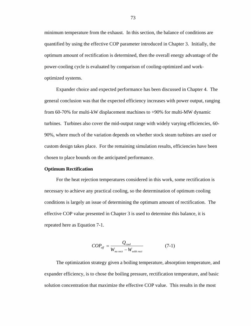
Optimum Rectification
For the heat rejection temperatures considered in this work, some rectification is
necessary to achieve any practical cooling, so the determination of optimum cooling
conditions is largely an issue of determining the optimum amount of rectification. The
effective COP value presented in Chapter 3 is used to determine this balance, it is
repeated here as Equation 7-1.
rectwithrectno
cooleff WW
QCOP
−= (7-1)
The optimization strategy given a boiling temperature, absorption temperature, and
expander efficiency, is to chose the boiling pressure, rectification temperature, and basic
solution concentration that maximize the effective COP value. This results in the most
74
energy effective trade-off of work and cooling production given the specified inputs.
Figure 7-1 is a plot of the maximum effective COP as a function of boiling temperature.
2.5
3
3.5
4
4.5
5
60 65 70 75 80 85 90 95 100
Boiling Temp. [C]
Eff.
CO
P
Expander Efficiency = 60 %
90 %
Figure 7-1. Maximum effective COP values where the work component is the amount of
work lost due to operation with rectification vs. equivalent conditions with no rectification.
The results of the maximum effective COP appear quite good. In the best cases,
the work that is lost due to rectification penalties is effectively traded for 4-5 times the
quantity of cooling. This is better performance than most conventional cooling systems,
however, it is not quite the complete picture of energy efficiency since work production
can also be optimized.
Overall Optimum Cooling
For a given heat source temperature, work optimization results in the system
configuration evolving toward a pure component working fluid Rankine cycle, that is a
high ammonia concentration in the basic solution. General optimum characteristics for
75
the power-cooling cycle have already been discussed and a brief comparison of the two is
given in Table 7-1.
Table 7-1. Typical operating characteristics for cooling and work optimized cycles. Optimization Vapor Mass Flow Fraction Basic Solution Concentration Cooling 5-10 % approx. 0.50 Work +90 % approx. 0.95
For a more stringent evaluation, cooling production can be assessed by the amount
of lost work that could be obtained from a work-optimized system. When considering
this scenario the overall effective COP has the following formulation.
/
/
/
1
cool c woverall
work optwork opt w cool
w cool
Q RCOPW W η
η
= =− ⎛ ⎞
−⎜ ⎟⎝ ⎠
(7-2)
Where the subscripts work opt and w/cool refer to parameters for the work
optimized case and those with cooling production, respectively. The rightmost
formulation represents the actual implementation with dimensionless parameters. The
term Rc/w is the ratio of cooling to work.
Figure 7-2 presents the maximum values of the overall, effective COP as a function
of boiling temperature. Based solely on energy considerations and the assumptions
inherent to Figure 7-2, at the best conditions nearly equal amounts of work must be
forfeited for the amount of cooling gained. The ratio of cooling to net work output is also
presented in Figure 7-2 to provide the relative magnitudes of each.
Exhaust Temperature
The exhaust temperature will determine suitable cooling applications, e.g. space
conditioning vs. refrigeration. The corresponding temperatures for the optimized cooling
cases of Figure 7-2 are presented in Figure 7-3.
76
0.5
0.6
0.7
0.8
0.9
1
1.1
1.2
1.3
1.4
60 65 70 75 80 85 90 95 100
Boiling Temp. [C]
Eff.
CO
P
0
0.2
0.4
0.6
0.8
1
1.2
Rat
io o
f Coo
ling/
Net
Wor
k O
utpu
t
Eff. COP
Cooling/Work Ratio
60% = Expander Efficiency
90%
90%
60%
Figure 7-2. Maximum overall effective COP values as defined by Equation 7-2.
-10
-5
0
5
10
15
60 65 70 75 80 85 90 95 100
Boiling Temp. [C]
Exh
aust
Tem
p. [C
]
Expander Efficiency = 90 %
60 %
Figure 7-3. Corresponding exhaust temperatures for the optimum conditions presented in
Figure 7-2.
77
However, these values are complicated by numerically maximizing the effective
COP values and do not provide a complete picture of the exhaust temperatures attainable.
Consideration of the relationship between overall effective COP and other system
parameters provides a better indication of achievable exhaust temperatures. Figure 7-4
attempts to show this relationship by plotting results of constant temperature operation in
a boiling pressure-basic solution concentration plane. Three parameters are plotted in
Figure 7-4: the overall effective COP value, the expander exhaust temperature, and the
vapor mass flow fraction (mvr/ms). The maximum effective COP value is centered within
the 1.08 isoline at approximately a pressure of 1.03 MPa and a basic solution
concentration of roughly 0.46. The corresponding exhaust temperature and vapor flow
fraction is -4.5° C and 7.8%, respectively. Figure 7-4 shows that the effective COP is
much more sensitive to the vapor flow fraction than the exhaust temperature. Therefore,
with a mild penalty to effective COP values, a large range of exhaust temperatures could
be accessed. For example, while operating within the 1.08 effective COP isoline, the
exhaust temperatures could vary between approximately -7° C and -2.3° C. Furthermore,
if the effective COP were diminished by 7.5% (the 1.0 isoline), the range of possible
exhaust temperatures would be between roughly -12° C to 5.6° C.
Implementation
The preceding results identify preferred conditions for cooling production. In this
section some of the implications of these conditions are considered as they relate to
physical implementation of the power-cooling cycle.
78
0.5
0.8
1.1
1.4
1.7
0.4 0.44 0.48 0.52 0.56 0.6
Basic Solution Concentration
Boi
ling
Pre
ssur
e [M
Pa]
Vapor Mass Flow Fraction = 0 %5 %
10 %
15 %
1.08
1.0
OverallEffectiveCOP = 0.9
0.7
9o = Exhaust Temp. [C] 4.5o
0o
-4.5o
-7o
-10o
Figure 7-4. Design point map showing the relative sensitivity of overall effective COP to
vapor mass flow fraction and exhaust temperature. Sensitivity to mass flow is high, while with a mild penalty to effective COP a wide range of temperatures could be expected. Boiling temperature of 80° C.
Vapor Quality
Considering the optimum cooling conditions, certain regions may cause exit quality
concerns. Combinations of high boiling temperatures, high expander efficiencies, and
effective cooling production result in relatively low equilibrium exhaust qualities, 90-
95%. This is due to the fact that at these conditions the entropy of the vapor is low
enough that it can be expanded to conditions that have significant condensation.
It was concluded in Chapter 4 that dynamic machines, turbines, were the better
expander choice for medium to large work outputs. However, these machines are
sensitive to vapor quality, in terms of both operating efficiency and erosion damage.
79
From examination of steam turbine performance, the effect of vapor quality on
machine efficiency is mild, for example an exit quality of 90% would result in an
expected efficiency penalty of 5-10% [50]. On the other hand, erosion of flow path
components is a significant concern since it could require machine rebuilding or
replacement. For these cases cooling may have to be curtailed, either by limiting
rectification or superheating, to avoid unacceptable conditions.
Rectifier Implementation
It was pointed out in Chapter 3 that the physical setup of the rectification process
can have an effect on the penalties to work production because it can affect the quantity
of vapor that continues on to the expander. Here, these effects are reconsidered in light
of the conclusions regarding optimum rectification.
In Chapter 3 upper and lower bounds were placed on the efficiency of the
rectification process. It was pointed out that with high amounts of rectification, lower
rectifier exit temperatures, the difference between the two becomes excessive while there
is not a significant difference with minimal rectification.
The effects of minimum and maximum rectifier efficiencies on the optimum overall
effective COP is shown in Figure 7-5. From the figure it can be seen that compared to
the minimum performance case, an approximate 20% improvement could be obtained for
most conditions. This benefit will be weighed against the added complexity of a direct
contact heat exchanger.
Experimental Observations
Correlation of the experimental results to simulated data revealed unexpected and
unaccounted trends in system operation. Many of these deviations overshadowed the
80
basic operating mechanisms that were studied analytically. This section explains these
deviations and any impact on system design.
0.4
0.6
0.8
1
1.2
1.4
60 65 70 75 80 85 90 95 100
Boiling Temp. [C]
Ove
rall
Eff.
CO
P
0
10
20
30
40
50
Eff.
CO
P In
crea
se [%
]
COP with max. possible rectified vapor production
COP with minimum rectified vapor production
% Increase
Figure 7-5. Effect of the minimum and maximum bounds of rectifier operation on
effective COP values.
Absorption Pressure
The experimentally measured absorption pressure was higher than that predicted by
using saturation properties at the basic solution concentration and the measured
temperature. This is not surprising since previous experimental investigation [70]
showed similar results. However, part of the explanation is an unexpected coupling
between the boiling temperature and basic solution concentration. Basic solution
concentration increased with temperature, thus increasing absorption pressure, due to the
storage of weak solution in the separator.
81
At steady state operation all of the ammonia and water leaving the absorber are
returned to it so that the concentration of the solution in the absorber remains fairly
constant. It would be expected then, even at different operating conditions, that the
concentration remains at its original value. However, in the experimental setup there is
some stored liquid in the separator that causes this scenario to be out of balance. The
liquid is retained to form a vapor seal in the separator and amounts to approximately 25%
of the total working fluid mass. This is weak solution liquid, which is a larger percentage
water than the basic solution, so by basically removing it from the working fluid, the
basic solution concentration inevitably increases. Furthermore, the weak solution
concentration is dependent on the boiling temperature and this results in the coupling
between boiling temperature and basic solution concentration. A formulation of this
effect is given as Equation 7-3.
__ 1
basic orig weakbasic new
x yxx
y−
=−
(7-3)
Where the new basic solution concentration, xbasic new, is dependent on the original
concentration, xbasic orig, the current weak solution concentration, xweak, and the fraction of
the total mass of working fluid that is stored, y. The effect is plotted in Figure 7-6 as a
function of both boiling temperature and stored fraction. Also included in the figure are
experimental measurements of the basic solution concentration at the approximate
amount of storage.
As shown in Figure 7-6, the change in basic solution concentration is more
pronounced with higher boiling temperatures and stored fractions. Accounting for this
effect when determining absorption pressure, Figure 7-7, explains much of the difference
82
when simply assuming a constant concentration, 0.35 for this case. The remainder of the
difference is attributed to non-equilibrium performance of the absorber.
0.3
0.35
0.4
0.45
0.5
0.55
0.6
0 10 20 30 40 50 60
Stored Fraction [%]
Stro
ng C
once
ntra
tion
60C Measurement80C Measurement100C Measurement
Simulated data boiling temp. = 100 C
80 C
60 C
Figure 7-6. Computed effect of weak solution storage on basic solution concentration.
Experimentally measured basic concentrations also shown.
The crucial effect of absorption pressure on cooling production has been
mentioned, lower pressures are certainly preferred. Therefore, if not taken into account,
an undue pressure rise caused by this effect could limit cooling production. The obvious
solution, according to Figure 7-6, is to minimize the stored fraction.
83
0.1
0.12
0.14
0.16
0.18
0.2
0.22
0.34 0.35 0.36 0.37 0.38 0.39 0.4 0.41
Strong Concentration
Abs
orbe
r Pre
ssur
e [M
Pa]
Computed Equlibrium Pressures
Measured Absorber Pressure (+/-0.538 kPa)
Figure 7-7. Computed absorption pressures taking into account the changes of basic
solution concentration compared with measured absorber pressures.
Rectifier Pressure Effect
An unanticipated decrease in boiling pressure occurred between operations with
and without the rectifier, Figure 7-8. The drop in pressure was due to condensation of
vapor in the rectifier, which essentially behaved as a second outlet (the first being the
expander) for the high pressure vapor. Consistent with this explanation is the observation
that the pressure drop is most severe for the cases that have the highest amount of
condensed vapor. Figure 7-9 is a plot of the corresponding amounts of condensed vapor
for the same tests presented in Figure 7-8. For the points without rectification the vapor
lost between the separator exit and expander inlet is near zero or is zero as expected.
However, for the cases with rectification the amount of vapor condensed in the rectifier
increases with boiling temperature. Considering both Figures 7-8 and 7-9, the maximum
84
pressure drop was approximately 0.058 MPa where roughly 30% of the vapor produced,
was condensed.
0.3
0.35
0.4
0.45
0.5
0.55
50 55 60 65 70 75 80 85 90 95 100
Boiling Temperature [C]
Boi
ling
Pre
ssur
e [M
Pa]
Boiling P with rectification (+/-2.24 kPa)Boiling P no rectification (+/-2.24 kPa)
Figure 7-8. Measured drop in boiling pressure due to rectifier operation.
Using average values for the worst case, nominally 95° C, the effect on the rectified
vapor concentration amount to a decrease of 0.05% and a reduction in isentropic enthalpy
drop of 1.7%. These are somewhat minor, the largest impact, however, was a reduction
of 4% in vapor mass flow rate. This extra flow rate loss stems from the lower
concentration vapor that is produced as a result of the lower pressure boiling condition.
Because of the lower concentration vapor, 4% more of it is condensed in the rectifier as
compared to the vapor that would have been generated if the pressure remained high.
Again, this was a slightly unexpected effect and emphasizes the point that the vapor
“escaping” through condensation in the rectifier should accounted for in a system design.
85
0
5
10
15
20
25
30
35
50 55 60 65 70 75 80 85 90 95 100
Boiling Temp. [C]
Con
dens
ed V
apor
in R
ectif
ier [
%]
Vapor condensed, with rectification
Vapor condensed, no rectification
Figure 7-9. Amount of the produced vapor that was condensed in the rectifier. This data
corresponds to the results of Figure 7-8.
Conclusions
The parameters affecting cooling with this cycle have been identified and
thoroughly examined both analytically and experimentally. Operating trends have been
verified and unforeseen effects identified from experiments. A demonstration of sub-
ambient expander exhaust has been provided which to a limited extent, demonstrates the
key concept of the power-cooling cycle. Based on these cumulative investigations the
practical operating region for cooling production has been outlined and preferred
operating procedures identified. The final conclusions are summarized as follows.
• In determining the optimum degree of rectification the trade-off between work sacrificed and cooling gained can be used. This effective coefficient of performance can be as high as 5 for the cooling gained relative to the work lost due to the rectifier.
86
• When considering the impact of cooling production on the optimum amount of work that could be produced, however, the equivalent effective COP is lower with maximums near 1.1.
• Characteristics of this overall optimum include basic solution concentrations of 0.40-0.55 and vaporization fractions of 5-10%. Minimum expected temperatures are in the range of -4.5° C. However, with an approximate 10% penalty to the overall effective COP an 18° C range of exhaust temperatures can be accessed.
• As for expander implementation, in the smaller size range, displacement machines have advantages over turbines and have reached +70% efficiencies with comparable operation with steam. In large applications there are examples of dynamic turbines operating with ammonia-water and achieving +90% efficiency. Applications in the mid-range will likely be relegated to lower efficiencies, 60-80%, without resorting to custom designs in which case estimates of 90% efficiencies have been put forward.
• At combinations of high heat source temperatures and optimum cooling production with high efficiency expander operation (typical of dynamic machines at larger sizes), condensate formation in the expander is predicted to be greater. For these cases, cooling production may need to be curtailed to avoid efficiency penalties in the expander and possible erosion damage.
• An approximate 20% increase in the overall effective COP value could be expected by incorporating a boiler-rectifier system that more closely approximates the maximum theoretical amount of vapor production.
• When off-performance effects are taken into account, most of the operating trends have been confirmed by the experimental results. Additionally, aside from the noted exceptions, the simulation modeling does a reasonable job of estimating some experimentally measured parameters such as vapor flow rate and concentration.
• Simple equilibrium modeling of the absorber is not sufficient to predict the absorption pressure. A portion of this difference is caused by the change in basic solution concentration due to storage of weak solution. This effect is more pronounced at higher boiling temperatures and larger stored fractions.
• The condensation of vapor in the rectifier essentially acts as a secondary exit for the vapor thus lowering the boiling pressure when compared to equivalent cases without rectification. For the worst case encountered the pressure decrease was 0.058 MPa and this caused a corresponding 4% decrease in vapor mass flow rate.
• The apparent efficiency of the turbine used in the experimental work seemed to get worse as optimum conditions for cooling were approached. No conclusive reason has been identified except for unaccounted heat transfer either from the inlet vapor or to the exhaust stream.
87
It is difficult to quantify all of the advantages and disadvantages that the power-
cooling concept has in comparison to other options. However, the characteristics
described in this work can be used to evaluate the energy effectiveness of the power-
cooling concept. Furthermore, several design and modeling issues have been raised so
that they will be available for the next generation of studies into this concept.
88
CHAPTER 8 RECOMMENDATIONS
The previous chapter presented the cumulative results of this work. Considering
those as a preface, the current chapter explores future suggestions for the power and
cooling concept.
Experimental Testing
In retrospect the most severe underestimation when designing the experiments for
this work was the impact of the small vapor flow rate on expander operation. Not only
did this complicate the selection of a suitable device, but it resulted in a correspondingly
small power output that was difficult to measure.
It can be inferred from Chapter 4, which concerns expander design considerations,
that the expander used for this work was not the best choice in terms of performance. It
was, however, a choice between relative performance among tested expanders and
adaptability to the ammonia-water working fluid. Had the anomalies previously
discussed not occurred, the conditions were set to have a more dramatic demonstration.
For the small size of the current setup and likely any other prototype, the
recommendation would be to use a displacement expander rather than the dynamic
machine used in this work. At the outset of this work, the dynamic machine which was
eventually used had certain practical advantages over the displacement devices being
considered. Primarily these were simpler operation with adequate efficiency, no need for
oil, no shaft seal, and a very simple loading mechanism. However, considering the
89
difficulties encountered with making an accurate power output measurement, the
complications of displacement machines seem quite manageable.
Power measurements were complicated by two factors, the first is that small
amounts of inadvertent heat transfer (losses to the environment) could cause significant
errors in the computation of power produced based on thermodynamic measurements.
Secondly, the small quantity of power produced quite a small reaction torque (this was
complicated further by the high shaft speeds) that was difficult to measure accurately.
Increased flow (larger potential output) would improve things by making the expander
inlet/exhaust states less sensitive to heat transfer losses. Also with a larger power output,
direct measurements of the reaction torque could be simplified. This could also be
improved if the shaft speeds were lower, as might be the case with a displacement
expander.
Aside from a more efficient expander, the current experimental system would
benefit most from improved solution pump performance. Under the best circumstances
the measured flow rate (approximately 0.5 gpm) was less than half of the rated capacity
of the pump (1.3 gpm). With an increase in vapor production the boiler pressure would
rise for a given boiler exit temperature and nozzle configuration. This would be an
improvement for cooling production and likely even for the performance of the current
turbine. There appear to be two problems with the current pump configuration, the first
is the fact that the working fluid is at or very near saturation, so any significant pressure
drop could induce cavitation, secondly, the pump inlet piping from the absorber still
serves as a restriction.
90
Practical Application
In considering the possible applications of the power-cooling cycle, several facts
about cooling production need to be considered. Not the least of which is the
consideration of the amount of energy needed to produce cooling in this manner. The
overall effective COP values presented in Figure 7-2 indicate that nearly equal amounts
of work (that could have been produced with an optimized system) are sacrificed for
cooling produced. As suggested by those results and reemphasized here, cooling
production in this manner may not be as energy efficient as conventional work-driven
cycles. Therefore, it appears that for this concept to be useful, the convenience of
combined power and cooling will need to outweigh this disadvantage. Additional
thoughts concerning the future evaluation and possible application of the power-cooling
cycle follow.
ORC Comparison
From the conclusions of this work, it appears that any use of this concept will be
primarily as a power cycle with the secondary feature of cooling production. A solid
performance comparison of this cycle with the more-proven ORC technology would
likely give an indication for the potential use of this cycle. The ammonia-water based
power cycle was reintroduced by Kalina [23] to take advantage of the mixture’s boiling
temperature glide and reduce heat transfer irreversibilities when compared to steam
Rankine cycle operation. This advantage may be extended to lower operating
temperatures where organic Rankine cycles are typically employed, however, these fluids
generally have smaller latent heat values than water, so the advantage may be reduced or
even eliminated. A comparison of this power-cooling cycle and its chief competition,
organic Rankine cycles, would give an indication of its merit as a power cycle alone.
91
Another basis of comparison would be that ORC engines have proven, efficient
expander performance in small sizes, and the power-cooling concept may be at a
disadvantage in this area because of the lack of efficient designs, or evidence of them, for
ammonia-water. The underlying reasons for this were discussed in Chapter 4. The
opposite may be true for larger output systems where turbines for organic fluids would be
inordinately large, however, considering that most low temperature applications, solar
thermal, geothermal, etc., and the whole distributed generation concept have been
focused on small size ranges, this may be of little consolation.
Cooling Production
As for the cooling process itself, the cooling produced with this cycle is sensible
rather than latent. Therefore, analogous to the heat addition process, this may provide
some advantage in exergy efficiency. The suggestion here is that to effectively use the
cooling from this cycle, the temperature profile of the exhaust stream will have to be
taken into account. This will likely require counter-flow heat exchangers, but more
importantly it may reduce the heat transfer irreversibilities as compared to latent-based
cooling, which has an isothermal region. If this could be shown, then the argument could
be made that this sensible cooling could satisfy a load with fewer irreversible losses.
This could be a particular advantage when compared to absorption cooling cycles where
water (lithium-bromide system) and ammonia (aqua-ammonia system) are commonly
used as refrigerants. Both have high latent heats so the irreversibilities may be
significant.
As for applications for the cooling output, the obvious and immediate thoughts, for
example serving both the power and cooling needs of a residence, are likely not a good
match for the characteristics of the cycle. When the ratio of cooling to power and overall
92
effective COP values are considered, one realizes that the amount and cost of cooling is
not suitable for these traditional applications. For example, the quantity of cooling
produced is at most equal to the power output, but would typically be less to attain higher
operating efficiencies. This is almost the opposite of what the expected demand for a
residence might be. Furthermore, the cost of cooling, in terms of work that could have
been produced (overall effective COP), indicate that serving large cooling loads in this
manner may be inefficient.
Rather than these uses, it may be more fruitful to identify niche applications that
this cycle could be applied to. Applications should be considered where the cooling is
used internally in the power cycle itself to either improve overall performance or reduce
equipment count. For example, considering that the amount of cooling output can be just
a fraction of the work output, referring to the simulation results of Figure 3-3, a
configuration of the power-cooling cycle could be implemented where this fraction of
cooling could be used to keep the generator or other power conditioning device cool.
This could provide some performance improvement or simply eliminate the need for an
additional cooling system. This kind of practical advantage will need to be identified and
exploited.
Conclusion
Summing these considerations results in the power-cooling concept being a power
cycle that may be competitive with other heat engines and could produce small amounts
of cooling, or even intermittent cooling, with some cost to performance. Where
efficiency is of concern, a balance will need to be struck between the benefit associated
with cooling and the penalty incurred due to its production. The effective COP term can
be used to evaluate the suitability of modifying the expansion conditions to accommodate
93
cooling in this manner. Furthermore, possible applications for this cycle may include
those where cooling is not a primary output, but it is used to improve overall efficiency or
simplify implementation.
94
APPENDIX A PROPERTY EVALUATION
For the evaluation of the working fluid properties the method described by Xu and
Goswami [26] is employed. The Gibbs free energy method is used to determine mixture
properties while empirical equations for bubble and dew point temperatures are used to
determine phase equilibrium. Good agreement between this method and experimental
data have been shown [26].
Pure Component Properties
Beginning with the components needed to determine mixture properties, the Gibbs
free energy for a pure component is given as Equation A-1.
0 0 00 0
T P TP
PT P T
cG h Ts c dT dP T dTTν ⎛ ⎞= − + + − ⎜ ⎟⎝ ⎠∫ ∫ ∫ (A-1)
The subscript 0 indicates reference state properties. The empirical relations used
by Ziegler and Trepp [71] for constant pressure specific heat and specific volume are
used here, Equations A-2 through A-5.
Liquid phase relations:
21 2 3 4
l A A P A T A Tν = + + + (A-2)
21 2 3
lPc B B T B T= + + (A-3)
Gas phase relations:
232 4
1 3 11 11g CC C PRT C
P T T Tν = + + + + (A-4)
2
1 2 3gPc D D T D T= + + (A-5)
95
Substitution and integration of Equations A-2 and A-3 into Equation A-1 results in
the following expression for the reduced liquid phase Gibbs free energy.
double PTXs(double P, double T, double xa) { // Reduced Temps and Pressures Tr=T/Tb; Pr=(P*1000)/Pb; //Convert MPa to kPa before dividing // Ammonia mole fraction ya=xa/((xa/Ma+(1-xa)/Mw)*Ma); // Mixture molecular mass Mm=ya*Ma+(1-ya)*Mw; // Entropy of mixing smix=-R*(ya*log(ya+.000001)+(1-ya)*log(1.000001-ya)); // Gas phase properties sga=-R*(-sgroa-D1a*log(Tr/Troa)+D2a*(Troa-Tr) +0.5*D3a*(Troa*Troa-Tr*Tr)+log(Pr/Proa) +3*C2a*(Proa/pow(Troa,4)-Pr/pow(Tr,4)) +11*C3a*(Proa/pow(Troa,12)-Pr/pow(Tr,12)) +(11/3)*C4a*(pow(Proa,3)/pow(Troa,12)-pow(Pr,3)/pow(Tr,12))); sgw=-R*(-sgrow-D1w*log(Tr/Trow)+D2w*(Trow-Tr) +0.5*D3w*(Trow*Trow-Tr*Tr)+log(Pr/Prow) +3*C2w*(Prow/pow(Trow,4)-Pr/pow(Tr,4)) +11*C3w*(Prow/pow(Trow,12)-Pr/pow(Tr,12)) +(11/3)*C4w*(pow(Prow,3)/pow(Trow,12)-pow(Pr,3)/pow(Tr,12))); sgm=(ya*sga+(1-ya)*sgw+smix)/Mm; // Liquid phase properties sLa=-R*(-sLroa-B1a*log(Tr/Troa)+B2a*(Troa-Tr) +0.5*B3a*(Troa*Troa-Tr*Tr)+(A3a+2*A4a*Tr)*(Pr-Proa)); sLw=-R*(-sLrow-B1w*log(Tr/Trow)+B2w*(Trow-Tr) +0.5*B3w*(Trow*Trow-Tr*Tr)+(A3w+2*A4w*Tr)*(Pr-Prow)); sE=-R*(1-ya)*ya*(E3+E4*Pr-E5/(Tr*Tr)-2*E6/pow(Tr,3) +(E9+E10*Pr-E11/(Tr*Tr)-2*E12/pow(Tr,3))*(2*ya-1) +(-E15/(Tr*Tr)-2*E16/pow(Tr,3))*pow((2*ya-1),2)); sLm=(ya*sLa+(1-ya)*sLw+sE+smix)/Mm; return sgm, sLm; }
105
//////////////////////////////////////////////////////////////////////////////// Specific Volume
This subroutine returns values for the liquid and vapor phase specific volume.
Phase determination is handled in the calling program.
//////////////////////////////////////////////////////////////////////////////// double PTXv(double P, double T, double xa) { // Reduced Temps and Pressures Tr=T/Tb; Pr=(P*1000)/Pb; //Convert MPa to kPa before dividing // Ammonia mole fraction ya=xa/((xa/Ma+(1-xa)/Mw)*Ma); // Mixture molecular mass Mm=ya*Ma+(1-ya)*Mw; // Liquid specific volume components vLa=((R*Tb)/(Pb))*(A1a+A2a*Pr+A3a*Tr+A4a*Tr*Tr); vLw=((R*Tb)/(Pb))*(A1w+A2w*Pr+A3w*Tr+A4w*Tr*Tr); vLE=((R*Tb)/(Pb))*(ya*(1-ya)*(E2+E4*Tr+(E8+E10*Tr)*(2*ya-1) +E14*pow((2*ya-1),2))); vLm=(ya*vLa+(1-ya)*vLw+vLE)/Mm; // Vapor specific volume components vga=((R*Tb)/(Pb))*(Tr/Pr+C1a+C2a/(pow(Tr,3))+C3a/(pow(Tr,11)) +C4a*Pr*Pr/(pow(Tr,11))); vgw=((R*Tb)/(Pb))*(Tr/Pr+C1w+C2w/(pow(Tr,3))+C3w/(pow(Tr,11)) +C4w*Pr*Pr/(pow(Tr,11))); vgm=(ya*vga+(1-ya)*vgw)/Mm; return vLm,vgm; } ////////////////////////////////////////////////////////////////////////////////
106
APPENDIX B MODEL FORMULATION
The thermodynamic model used to generate the simulated results of this work is
described here. First, the individual component formulations are presented, and then the
implementation of these into programming code is presented.
Thermodynamic Formulations
The flow diagram used for the modeling is presented in Figure B-1. It is identical
to Figure 3-1 except now the individual state points have been numbered. Also
reproduced here is Table 3-1 (as Table B-1) which describes the stream labels in Figure
B-1. The assumptions and procedures outlined in Chapter 3, however, are not repeated
here, but it may be beneficial to review them in conjunction with the following
descriptions.
Formulation begins in the absorber where two inputs are given, the absorber exit
temperature and basic solution concentration. Assuming the basic solution is at or very
near saturation, property data is used to determine the system low pressure. System high
pressure is usually specified. With the pressure ratio known, an energy balance across
the pump yields Equation B-1.
( ) 1122 hhhh spump +−=η (B-1)
Using property data, state point 2 can be determined (using Pboiler, xs, and h2).
Moving to the boiler, where the pressure and temperature are known, the vapor and weak
solution ammonia mass concentrations and properties can be determined assuming
saturated conditions at boiler exit, states 5 and 6. Furthermore, the mass flow rates of
107
each are found from a mass balance of the boiler and saturated equilibrium conditions,
Equation B-2.
56
51
3
5
3
6 1xxxx
mm
mm
−−
=−=&
&
&
& (B-2)
HeatSource
Recovery HeatExchanger
Throttle
Boiler
Absorber Coolant
Separator
Coolant Rectifier
Expander
vr
SolutionPump
v
wb
w
wr
s
Superheater
HeatSource
Cooling HeatExchanger
CooledFluid
12
3
4 5 7
8
6
11
12
13
14
9 10
Figure B-1. Schematic used for the theoretical modeling.
Table B-1. Flow identification for the configuration of Figure B-1. Identifier/ Subscript
Description
s Basic (strong) solution flow from absorber through boiler v Vapor flow produced from partial vaporization in boiler vr Rectified vapor passing through turbine and cooling heat exchanger w Weak (in ammonia) solution liquid returning to absorber wr Weak condensate formed in rectifier wb Weak liquid produced from partial vaporization in boiler
108
With this information the boiler heat transfer is determined. From a boiler energy
balance Equation B-3 can be determined.
6 6 5 5 3 3boilerQ m h m h m h= + −& & & (B-3)
Note that at the moment the heat source medium is not taken into account, i.e. qboiler
represents only the amount of heat accepted by the system and does not account for the
efficiency or effectiveness of that heat transfer. Also note that state point 4 is not used, it
is assumed that it is a two-phase mixture which is divided into states 5 and 6.
Now computation proceeds to the rectifier where the vapor inlet state is known,
state 6, and the rectifier exit temperature is specified, T11. Also, points 7 and 11 are
interrelated through saturated equilibrium conditions, Equation B-6.
711
76
6
7
6
11 1xxxx
mm
mm
−−
=−=&
&
&
& (B-6)
There is now enough information to complete the rectifier energy balance and
determine the rectifier heat transfer using the following expression.
( )rectifier 6 6 11 11 7 7Q m h m h m h= − +& & & (B-7)
There is now enough information to return to the weak solution exit from the
boiler. At this junction the weak solution from the boiler, rectifier condensate, and
cooling strong solution are mixed. State 8 is determined from the junction mass and
energy balances, Equations B-8 and B-9.
8 3 7m m m= +& & & (B-8)
3 3 7 78
8
m h m hhm+
=& &
& (B-9)
109
For the recovery heat exchanger exit conditions, an effectiveness is assumed, and
based on the maximum heat transfer that can occur, the exit states can be determined.
Assuming counter-flow operation, the limiting exit conditions are either that T3 is raised
to T8 or T9 is cooled to T2 so the maximum heat exchange is the minimum of Equation B-
10.
( ) ( )max recovery 3 3max 2 8 8 9minmin of orQ m h h m h h= − −& & (B-10)
Subsequently, the recovery unit exit states are determined by Equations B-11 and
B-12.
recovery max recovery3 2
3
Qh h
mη
= +& (B-11)
recovery max recovery9 8
8
Qh h
mη
= −& (B-12)
Of course each end state above has the possibility of being a two phase mixture so
the enthalpies at those points, 3 and 9, should reflect mixture properties. The weak
solution throttle is assumed to be isenthalpic, Equation B-13.
109 hh = (B-13)
This completes the strong and weak portions of the cycle, now the vapor circuit can
be completed. The vapor entering the superheater is assumed to be saturated, state 11.
As with the rectifier operation, the superheater operation is determined by specifying the
exit temperature. Since pressure and concentration are also known, the other
thermodynamic properties can be determined. This brings computation to the inlet of the
expander. An isentropic expander efficiency is assumed and the exit conditions are found
through Equation B-14.
110
( )sturbine hhhh 13121213 −−= η (B-14)
Having determined the expander exit enthalpy, there is sufficient information to
determine its exhaust temperature (using Pabsorber, xvr, and h13). Based on this exhaust
temperature, the cooling heat exchanger may not be active if the temperature is not below
the limit specified for cooling production. For the analysis of cooling production this
threshold temperature was 15° C. If T13 is higher than this, then the cooling heat
exchanger has no effect. If the exhaust temperature is below the threshold the vapor is
heated to another specified temperature, typically the threshold temperature. This of
course fixes the properties at point 14 and the cooling obtained can be determined from
an energy balance of the cooling heat exchanger, Equation B-15.
( )13 14cooling vrQ m h h= −& (B-15)
Finally, all of the conditions needed to compute the heat rejected in the absorber are
know. From an energy balance of the absorber the rejected heat can be determined from
Equation B-16.
10 10 14 14 1 1absorberQ m h m h m h= + −& & & (B-16)
This concludes the calculations needed to solve for the conditions in this
configuration of the power-cooling cycle, attention is now turned to the coding of these
formulations for computer execution.
Computer Implementation
This section presents much of the computer code used to compute cycle operating
parameters. The subroutines that follow, which are built upon the fundamental property
routines presented in Appendix A, have been used in various combinations to compute
cycle performance. Along with the brief description preceding each routine,
111
determination of its function should be self-evident. Many of the routines are used to
determine properties using inputs other than pressure, temperature, and mixture
concentration (the inputs for the fundamental routines presented in Appendix A). To do
this an iterative search routine is used, which employs the bisection method.
Saturated Liquid Pressure
This subroutine computes the liquid saturation pressure given a temperature and
liquid concentration as inputs. It is typically called to determine absorber pressure since
basic solution concentration and absorption temperature are specified.
//////////////////////////////////////////////////////////////////////////////// double TXSatLiq(double T, double xa) { double Plmin=0.005; // Search interval, may need adjustment double Plmax=20; // P's in MPa double Plmid; double fPlmid=1; SatTemp(Plmax,xa); double fPlmax=Tbub-T; SatTemp(Plmin,xa); double fPlmin=Tbub-T; int i=0; while (sqrt(fPlmid*fPlmid) > .00001){ Plmid=(Plmin+Plmax)/2; SatTemp(Plmid,xa); fPlmid=Tbub-T; ++i; if (i > 100){ PsatL=0; return PsatL; } if ((sqrt(pow((Plmax-Plmin),2)))<0.0001){ PsatL=Plmax; return PsatL; } if ((fPlmin*fPlmid) <= 0){
112
// Root is in the left half interval Plmax=Plmid; fPlmax=fPlmid; } else { // Root is in the right half interval Plmin=Plmid; fPlmin=fPlmid; } } PsatL=Plmid; return PsatL; } //////////////////////////////////////////////////////////////////////////////// Two-Phase Mixture Determination
This routine computes the mixture quality and the vapor and liquid saturation
concentrations given the pressure, temperature, and the original solution concentration.
This routine is commonly employed to determine the mass flows and concentrations at
the separator exit, states 5 and 6. It is also used at the rectifier exit to determine states 7
and 11.
//////////////////////////////////////////////////////////////////////////////// double PTXsatx(double P, double T, double xv) { // Check for single phase SatTemp(P,xv); if (T<=Tbub){ xq=0; return xq; } if (T>=Tdew){ xq=1; return xq; } // Must be two-phase, begin searching
113
double xmin=0.01; // Search interval double xmax=1; double xLiq; double xGas; double xmid; double fxmid=1; SatTemp(P,xmax); double fxmax=Tbub-T; SatTemp(P,xmin); double fxmin=Tbub-T; int i=0; // Begin iterations to find xLiq, i.e. set T=Tbub while (sqrt(fxmid*fxmid) > .0001){ xmid=(xmin+xmax)/2; SatTemp(P,xmid); fxmid=Tbub-T; ++i; if (xmin<xmax){ if (i > 100){ xq=0; cout << "xLiq iteration limit" <<endl; return xq; } if ((fxmin*fxmid) <= 0){ // Root is in the left half interval xmax=xmid; fxmax=fxmid; } else { // Root is in the right half interval xmin=xmid; fxmin=fxmid; } } else { fxmid=0; } } xLiq=xmid; fxmid=1; // Reset search parameters
114
xmax=1; xmin=0.01; SatTemp(P,xmax); fxmax=Tdew-T; SatTemp(P,xmin); fxmin=Tdew-T; i=0; // Begin iterations to find xGas, i.e. set T=Tdew while (sqrt(fxmid*fxmid) > .0001){ xmid=(xmin+xmax)/2; SatTemp(P,xmid); fxmid=Tdew-T; ++i; if (xmin<xmax){ if (i > 100){ xq=0; cout << "xGas iteration limit" <<endl; cout << "P " << P << " T " << T << " xv " << xv <<endl; return xq; } if ((fxmin*fxmid) <= 0){ // Root is in the left half interval xmax=xmid; fxmax=fxmid; } else { // Root is in the right half interval xmin=xmid; fxmin=fxmid; } } else { fxmid=0; } } xGas=xmid; if (xLiq >= 1){ xq=1; }
if (i > 100){ xsatG=0; return xsatG; } if ((sqrt(pow((xmax-xmin),2)))<0.0001){ xsatG=xmax; return xsatG; } if ((fxmin*fxmid) <= 0){ // Root is in the left half interval xmax=xmid; fxmax=fxmid; } else { // Root is in the right half interval xmin=xmid; fxmin=fxmid; } } xsatG=xmid; return xsatG; } //////////////////////////////////////////////////////////////////////////////// Two-Phase Mixture Enthalpy
For those conditions that are in the two phase region, this routine computes the
mixture enthalpy given a pressure, temperature, and overall concentration. The quality of
hmix=hgm; xq=1; return hmix, xq; } else { PTXsatx(P,T,x); hmix=xq*hgm+(1-xq)*hLm; } return hmix,xq,hgm,hLm; } //////////////////////////////////////////////////////////////////////////////// Temperature Determination Using Enthalpy
This subroutine determines the fluid temperature from the input parameters of
pressure, concentration, and enthalpy. This is used in situations where the enthalpy can
be determined from an energy balance and the corresponding temperature is needed.
//////////////////////////////////////////////////////////////////////////////// double PXHmixT(double P, double x, double h) { double Tmin=100; // Search interval, T's in K double Tmax=800; double Tmid; double fTmid=1; mixh(P,Tmax,x); double fTmax=h-hmix; mixh(P,Tmin,x); double fTmin=h-hmix; int i=0; while (sqrt(fTmid*fTmid) > .0001){ Tmid=(Tmin+Tmax)/2; mixh(P,Tmid,x); fTmid=h-hmix; //cout << "Tmid " << Tmid << "Tmax " << Tmax << "Tmin " << Tmin <<endl; ++i; if (i > 100){
119
Tmix=0; //cout << "i>100 " <<endl; return Tmix; } if ((sqrt(pow((Tmax-Tmin),2)))<0.0001){ Tmix=Tmax; return Tmix; } if ((fTmin*fTmid) <= 0){ // Root is in the left half interval Tmax=Tmid; fTmax=fTmid; } else { // Root is in the right half interval Tmin=Tmid; fTmin=fTmid; } } Tmix=Tmid; return Tmix,xq; } //////////////////////////////////////////////////////////////////////////////// Isentropic Temperature Determination
This routine computes the resultant temperature given the inputs of pressure,
concentration, and entropy. It is typically used to determine the isentropic expander exit
temperature, which is then used with the conventional pressure, temperature,
concentration routine to determine the isentropic exhaust enthalpy.
PTXs(P,Tmax,x); double fTmax=s-sgm; PTXs(P,Tmin,x); double fTmin=s-sgm; int i=0; while (sqrt(fTmid*fTmid) > .00001){ Tmid=(Tmin+Tmax)/2; PTXs(P,Tmid,x); fTmid=s-sgm; ++i; if (i > 100){ TisenV=0; return TisenV; } if ((sqrt(pow((Tmax-Tmin),2)))<0.0001){ TisenV=Tmax; return TisenV; } if ((fTmin*fTmid) <= 0){ // Root is in the left half interval Tmax=Tmid; fTmax=fTmid; } else { // Root is in the right half interval Tmin=Tmid; fTmin=fTmid; } } TisenV=Tmid; return TisenV; } //////////////////////////////////////////////////////////////////////////////// Overall Cycle Calculation
By employing many of the subroutines just presented, this routine computes the
state point properties and other parameters given the boiling temperature, boiling
The experimental procedures have been described in Chapter 5, this section
provides the details needed to operate ancillary equipment.
Data Acquisition System
All of the data, aside from the manually recorded measurements, was collected with
a DaqBook 200 acquisition system. For hardware information refer to the equipment list
later in this Appendix, and for hardware configuration please refer to the operating
manual for the DaqBook system. The acquisition software used is called DaqView. In
this software each transducer is assigned a channel which can have its own calibration
factors, i.e. for a linear fit, a slope and intercept. The factors used for this purpose were
obtained by calibrating the transducers; these values are provided in the subsequent
sections. As for data collection, a sampling rate of 25 scans per second for one second
was used. The data was converted from binary-coded to ASCII format and saved as a
text file.
Gas Chromatograph
A gas chromatograph (GC) was used to analyze basic solution and weak solution
samples during experiments. The startup and settings for the GC are as follows.
1. Verify that the correct column for ammonia-water separation is installed.
2. The helium carrier gas supply tank is opened. All other valves leading to the GC are also opened. The regulator should be adjusted to approximately 60 psig. Gas flow past the thermal conductivity detector (TCD) can be verified by immersing the
128
exhaust tube from the TCD oven, which is located inside the main oven, into a small vial of water and observing bubbles leaving the tube.
3. Power is turned on to the data acquisition PC and the PC-GC interface. With the computer on, the GC software “PeakSimple” is started and the appropriate control file is loaded, “cycle.con”.
4. The GC itself can now be turned on and the settings verified. The on-board flow regulator should be set at 400. The TCD attenuator switch should be set to 1. Using the GC’s digital readout the following temperatures and pressures should be verified.
5. Carrier 1 pressure should be 50 psig
6. Head pressure 1 should be approximately 6-10 psig, pressures significantly different from this may require replacement of the injection septum.
7. Oven temperature set point of 100° C.
8. TCD set point of 125° C.
9. The filter bake switch on the GC is switched on.
10. The TCD current switch is switched to the high setting.
The GC should idle for approximately one hour or until the TCD output stabilizes.
Samples typically cleared the detector in under 8 minutes with these conditions, so this
was chosen as the length of the data acquisition cycle. Shutdown of the GC is the reverse
of startup.
Uncertainty of Direct Measurements
This section gives details of the measurement uncertainties and the computation of
the error bounds for the experimental data. A description of the experimental system has
been given in Chapter 5 and the equipment specification is provided later in this
appendix. For the results of concern for this work, there are five types of fundamental
measurements from which all other quantities are derived These are temperature,
pressure, concentration, volume flow rate, and expander shaft speed. Other
129
measurements were made when air-testing the expander, however, those measurements
are treated in separately in Appendix D.
Temperature
All temperatures were measured with type “T” thermocouples interfaced with a
DBK-82 thermocouple analog to digital card and a DaqBook 200 PC interface. A two-
point linear calibration (ice point and boiling point) was performed with all
thermocouples prior to installation. Table C-1 presents the computed slopes and
intercepts.
Table C-1. Calibration factors for the thermocouples used in this work. Probe Location Slope InterceptLetter Description [-] [C]
E Absorber Vapor In 0.997008973 -0.398803589F Absorber Weak In 1.005025126 -0.603015075D Absorber Strong Out 1.006036217 -0.704225352C Absorber Liquid Pool 1.004016064 -0.803212851K Boiler Strong In 1.004016064 -0.702811245L Separator Strong In 1.005025126 -0.703517588B Absorber Coolant In 1.005025126 -0.804020101A Absorber Coolant Out 1.004016064 -0.702811245M Boiler Heat Source In 1.006036217 -0.704225352Q Boiler Heat Source Out 1.004016064 -0.602409639J Rectifier Coolant In 0.998003992 -0.499001996I Rectifier Coolant Out 1 -0.6R Separator Weak Out 1.005025126 -0.703517588S Separator Vapor Out 1.001001001 -0.500500501T Expander Inlet 1.005025126 -0.703517588U Expander Exhaust 1.003009027 -0.702106319W Rectifier Vapor Out 1 -0.5
The accuracy of the thermocouple readings was improved by using the above
calibration constants, however, the repeatability of the entire measuring system was the
largest contributor to measurement uncertainty. Variations in measurement channels,
ambient conditions, etc., contributed to a total uncertainty of 0.4° C in all thermocouple
measurements.
130
Pressure
Pressure was measured with strain gage type transducers, the specific models are
listed in the equipment specification section. Similar to the thermocouples, each
transducer was calibrated before installation. An Ametek pressure tester (model HL-24,
serial HL-5886) was used to apply 5 different calibration pressures to each transducer
across its expected range of operation. Calibration constants, Table C-2, for each
transducer were determined from a linear regression of the five data points.
Three volume flow rates were recorded and used to determine mass flows in this
work, they are the basic solution flow, weak solution flow, and the turbine vapor flow.
The first two were measured with variable area rotameters while for the latter a turbine-
type flow meter was used.
131
The basic and weak solution rotameters have been calibrated for the volume flow
of liquids with specific gravities of 0.833 and 0.88 respectively. Equation C-1 is used to
correct the indicated reading to the actual volume flow.
( )( )
float act calact ind
float cal act
Q Qρ ρ ρ
ρ ρ ρ
−=
− (C-1)
Where the float density is the same for both meters, 8016 kg/m3, which corresponds
to 316 stainless steel. The accuracy is stated as ± 1 % of full scale for the range 0.1 to
1.11 gpm for the basic solution meter and ± 1 % of full scale for the range 0.08 to 0.8
gpm for the weak solution meter.
The turbine-type flow meter used for vapor flow measurements directly measures
volume flow rate, therefore, no correction for calibrated conditions is needed. Accuracy
is given as ± 1 % of reading. The output of the meter is a 4-20 mA signal proportional to
the flow rate. The constants used in the data acquisition software were a slope of
6.1248569489 and an intercept of -6.250.
Concentration
Direct ammonia concentration measurements were taken at two points in the
system, the basic solution flow and the weak solution flow. A gas chromatograph (GC)
with a thermal conductivity detector (TCD) calibrated for detecting ammonia-water was
used to make these direct measurements. Both of these streams are liquids. This method
proved unsuitable for saturated vapor concentration measurements, therefore, vapor
concentration is derived from pressure and temperature measurements, details in a later
section.
132
The GC was calibrated with a concentration standard to determine the calibration
constants and measurement uncertainty. Repeated measurements were taken of a sample
containing an ammonia mass fraction of 28.76 %, per the certificate of analysis provided
by the chemical supply company. The output of the GC is a plot of TCD voltage versus
time; distinct peaks in voltage are recorded for each constituent component, ammonia and
water. The quantitative output is the ratio of the area under the peak corresponding to
ammonia to the entire area under all peaks and is related to the ammonia mass fraction
through equation C-2.
( )3% 100
1 1NHCxA
C x=
− + (C-2
The calibration constant, C, was computed as the average of the constants
computed for each measurement of the standard solution using equation C-3.
33
2 3
1
0
%1100 %
c
c
NHNH x xx c
cH O NHx x x
AA xCxA A
==
= =
⎛ ⎞⎛ ⎞− ⎜ ⎟= = ⎜ ⎟⎜ ⎟−⎝ ⎠⎝ ⎠
(C-3)
The average calibration constant computed from 15 measurements was 0.9794.
The uncertainty in concentration measurements using a 95 % confidence interval is ±
0.015.
Shaft Speed
The optical speed sensor has been described previously. Measurement uncertainty
based on the deviation of repeated measurements is ± 94 rpm with a 95 % confidence
interval. Due to the sensor’s design, it registered two pulses per revolution, therefore, a
scale factor of 30 was used in the data acquisition software to obtain readings in
revolutions per minute.
133
Uncertainty of Derived Measurements
To determine the accumulated error in derived measurements, those quantities that
are functions of two or more primary measurements, the square root of the sum of the
squares of the individual contributing errors is used. A derived quantity y can be written
in terms of the primary measurements x in general form as equation C-4.
( )1 2, , , ny f x x x= L (C-4)
Assuming independent and symmetrical errors in the primary measurements, dx,
the error in the derived parameter, dy, can be estimated from equation C-5.
22 2
1 21 2
nn
y y ydy dx dx dxx x x
⎛ ⎞⎛ ⎞ ⎛ ⎞∂ ∂ ∂= + + + ⎜ ⎟⎜ ⎟ ⎜ ⎟∂ ∂ ∂⎝ ⎠ ⎝ ⎠ ⎝ ⎠
L (C-5)
Many of the derived quantities depend on the fundamental measurements used with
thermodynamic property data of ammonia-water. Since these relationships cannot be
directly differentiated as indicated in equation C-5 a finite difference numerical scheme is
used to approximate them. The formulation for the central-difference approximation,
neglecting higher order terms, is presented as equation C-6.
( ) ( )1 2 1 2, , , ( ) , , , ( )2
n n n n
n n
f x x x dx f x x x dxyx dx
+ − −∂=
∂L L
(C-6)
The following paragraphs describe the derived measurements used in this work,
they present the dependence on direct measurements and give the uncertainty values
used.
Vapor Concentration
Syringe sampling and GC analysis proved unsuitable for vapor flow measurements
because the vapor is saturated at the sampling location. Despite the precaution of heating
134
the syringe, condensate inevitably formed and remained in the needle after injection into
the GC. On the other hand, there is always at least one location where the vapor is
confidently considered saturated and separated from liquid, the separator exit and the
rectifier exit when the rectifier is in operation. Therefore, it was decided to use the
proximate temperature and pressure measurements and an assumption of saturated
conditions to determine concentration from thermodynamic property data.
Vapor concentration = f (pressure, temperature) (C-7)
Mass Flow Rates
The strong and weak flow rates are determined from the direct measurements of the
volume flow rate, temperature and concentration. The thermodynamic properties are
used to compute a density which converts the volume flow measurements to mass flow
readings. For error analysis the functional dependence of the basic and weak mass flow
rates is the following.
Basic/Weak mass flow = f (volume flow, concentration, temperature) (C-8)
Note that the pressure dependence on mass flow is neglected for these liquid flows.
As for vapor mass flow determination, the functional dependence of measurements
directly related to the measured volume flow is similar to the ones above.
Vapor mass flow = f (vapor volume flow, pressure, temperature, concentration)
(C-9)
Note, however, that the errors due to uncertainty in the pressure reading need to be
accounted for in this case. Also, this flow has been generically termed the vapor mass
flow, which is the flow measured by the vapor flowmeter. This is distinguished from the
flow entering the rectifier (when in operation), which is not directly measured. Rather, it
is derived from a mass balance of the rectifier, since both vapor inlet and outlet states are
135
assumed saturated and the concentration is known. The functional dependence for this
stream is then given as the following.
Rectifier inlet vapor mass flow = f (vapor volume flow, pressure, temperature, inlet
and outlet concentrations) (C-10)
Power Output
For expander operation in the power-cooling setup, power output was estimated
from the thermodynamic states at turbine inlet and exhaust. Mechanical measurements
were used for some air testing, however, that analysis is treated separately in Appendix
D. Power output is then dependent on the following parameters, of which the
dependence on direct measurements has been discussed.
Power output = f (vapor mass flow, vapor concentration, inlet and exhaust
temperatures and pressures) (C-11)
Expander Efficiency
Based on the just-described, derived measurement, the expander efficiency is
determined from two power output measurements as shown in the following.
Expander efficiency = f (Computed power output, Ideal computed power based on
measured conditions) (C-12)
The resulting uncertainties along with a summary of the functional dependencies
are presented in Table C-4.
136
Table C-4. Derived measurement uncertainty summary. Parameter Error Dependence Uncertainty Rectifier Exit Vapor Conc. P, T ± 0.00031 kg/kg Separator Exit Vapor Conc. P, T ± 0.00067 kg/kg Basic Solution Mass Flow Q, T, X ± 0.00062 kg/s Vapor Mass Flow Q, T, P ± 0.00003 kg/s Rectifier Inlet Vapor Mass Flow Q, T (2), P (2) ± 0.000048 kg/s Power Output Q, T (2), P (2) ± 1.6 W Expander Efficiency Q, T, P (2) ± 5.4 %
Equipment Specification
This section details the measurement equipment and expander used for this work.
For details regarding the physical makeup of the rest of the experimental setup, which is
not covered in detail here, the reader is referred to the description given in Chapter 5 or
reference [70].
Instrumentation
The pertinent descriptive information about the measurement equipment used is
detailed in Table C-5.
Table C-5. Detailed descriptions of the instrumentation and measurement equipment used for this work.
Device
Manufacturer
Part Number/Model
Vendor (if known)
Data Acquisition PC Interface
IoTech
DaqBook 200 Ser. 219024
IoTech (440) 439-4091
Frequency Measurement Card
IoTech
DBK 7
IoTech (440) 439-4091
Current/Voltage Measurement Card
IoTech
DBK 15
IoTech (440) 439-4091
Thermocouple Measurement Card
IoTech
DBK 82
IoTech (440) 439-4091
All Temperatures T-type Thermocouples
Omega
TMQSS-125U-6
Omega (800) 826-6342
Pressure Transducers Absorber Exit, 2
Cole Parmer
Model 68073-04 Ser. 1490231
Cole Parmer (800) 323-4340
137
Table C-5. Continued. Device
Manufacturer
Part Number/Model
Vendor (if known)
Pressure Transducers Vapor Throttle Exit, 3 Cole Parmer Model 68073-04
Ser. 1490230 Cole Parmer (800) 323-4340
Absorber Vapor Inlet, 4 Cole Parmer Model 07356-13 Ser. 00205
Cole Parmer (800) 323-4340
Absorber Weak Inlet, 5 Cole Parmer Model 68073-06 Ser. 1853374
Cole Parmer (800) 323-4340
Separator Entrance, 6 Setra Part # SE256103 Model 256 Ser. 0903 1945647
Davis Inotek Instruments (800) 368-2516
Turbine Inlet, 7 Setra Part # SE256103 Model 256 Ser. 0903 1945648
Davis Inotek Instruments (800) 368-2516
Turbine Exhaust, 8 Cole Parmer Model A-68073-04 Ser. 1945762
Cole Parmer (800) 323-4340
Flowmeters Vapor, Turbine-type Hoffer Flow
Controls, Inc. Model HO3/4X3/4-20-CB-1MC3PAX8S-NPT Ser. 99628
Quinn Associates (813) 254-5211
Basic Solution, Rotameter Brooks Model 1110DJ33C4DAA Serial 0199120123644/001
Weak Solution, Rotameter Brooks Model 110CJ32CMDAA Serial 9812HC028152/1
Gas Chromatograph SRI Model 8610-50
Serial 1027 Column HAYSEP T
Expander Details
The expander used for these experiments was a converted turbine originally used in
an aircraft air-cooling system. The units were manufactured by Airesearch
manufacturing and have a factory part number of 56690. Components from three
138
turbines were used in this work and they were obtained from C and H sales (800) 325-
9465, under the part number DCB2410.
Some modifications were needed to adapt this device for service in the
experimental setup. Most notably this involved the manufacture of a new rear housing
since the original had vents to the atmosphere. The drawings that follow give an
overview of the parts manufactured (by the author) to form a sealed rear housing and
adapt the turbine for service with ammonia-water working fluid. First is figure C-1
which shows the complete assembly.
Figure C-1. View of the assembled rear housing.
Figure C-2 is an exploded view of the assembly with the individual parts labeled.
The spindle and the rotor were used as-removed from the original turbine. The back
plate, housing, and front plate were all manufactured for this work.
139
Figure C-2. Exploded view of the rear housing assembly.
Back Plate
Housing
Spindle
Front Plate
Rotor
140
APPENDIX D EXPANDER AIR TESTING
It was mentioned in the earlier chapters of this work that the turbine used for the
experiments was also tested with air to resolve some of the performance measurement
discrepancies. Indeed, Figure 6-7 contains data from these tests and is used to eliminate
some of the questionable results. This appendix provides the experimental details for
those measurements based on air tests.
Experimental Setup
Figure D-1 is a schematic of the setup used for air testing. Compressed air was
supplied by a standard shop air compressor at approximately 90 psig. An adjustable
pressure regulator was used to control the flow and expander inlet pressure. On the inlet
line two parallel rotameters were used to measure volume flow rate (two were used
because the flow exceeded the capacity of a single meter), and a pressure transducer
monitored inlet pressure. The same thermocouples used in the ammonia-water
experiments were used here to record inlet and exhaust temperatures. The expander
speed sensor was described in Chapter 5 and was used here. Also, the same data
acquisition system used for the ammonia-water experiments was used for these tests.
Note in Figure D-1 that two options were used to absorb the mechanical power
produced by the expander. One is the magnetic brake device that was described in
Chapter 5 and used for the ammonia-water experiments. Figure D-2 is a photograph of
the rear of the expander showing the aluminum disk that was used in the magnetic brake
arrangement.
141
T
T
Expander
From AirCompressor F
PressureRegulator
P
Exhaust toAtmosphere
MagneticBrake
GearboxGenerator
TorqueMeasurement
SpeedMeas.
Figure D-1. Setup schematic used for the air testing.
Figure D-2. Rear view of expander with cover removed. The aluminum disk used with
the magnetic brake is visible.
142
Figure D-3. Photograph of generator loading arrangement.
The other loading configuration is one that allowed a direct measurement of the
power produced. It consisted of a DC permanent-magnet generator driven by the
expander through a reducing planetary gearbox (6:1), Figure D-3. The generator was
mounted in such a way that it was constrained from rotating by a load cell link. This
provided a measurement of the torque supplied to the generator and along with the shaft
speed measurement was used to compute a torque-based power measurement (power =
Load Cell
Generator in reaction torque frame
Turbine
143
torque × angular momentum). The torque measurements were used to confirm the power
computed from the thermodynamic measurements. A photograph of the generator
mounting arrangement is shown in Figure D-3. Figure D-4 shows the gearbox mounted
inside of the expander housing.
Figure D-4. Photograph of gearbox mounted on expander spindle.
Test Results
Tests were performed to verify the thermodynamic method of computing power
and to provide a measure of the expander’s no-load power consumption. Initially, testing
was performed in the same manner as with ammonia-water. The pressure regulator was
Gearbox
Spindle Housing
144
used to maintain a desired inlet pressure, then beginning with the no-load condition the
turbine was progressively loaded in incremental steps. Measurements were made at each
loading step. The results were used to compute the expander power via the two methods,
thermal and torque-based. Results from a test with a nominal inlet pressure of 40 psig are
shown in Figure D-5.
0
10
20
30
40
50
60
70
80
90
20000 25000 30000 35000 40000 45000 50000
Shaft Speed [rpm]
Turb
ine
Pow
er [W
]
Thermal Meas.Torque Meas.
Figure D-5. Air testing results comparing the value of power that was computed by the
thermal-based and torque-based measurements.
As shown in Figure D-5 there is a fairly constant difference between the two
methods at lower shaft speeds (approximately 24 krpm to 32 krpm), while at higher
speeds the difference grows dramatically with the thermal measurement indicating higher
outputs.
This difference has a plausible explanation which is, at higher speeds more of the
power removed from the working fluid is consumed within the turbine and does not show
145
up as torque on the generator. The internal loads of the turbine consist largely of the
friction in the bearings and the fluid friction caused by the drag on the rotating parts of
the expander.
To test this theory, tests were performed to measure the internal power
consumption of the expander. This was accomplished by removing all external loading
from the expander and measuring conditions at the no-load speed. Different speeds were
obtained by adjusting the pressure regulator, which controls the inlet pressure. For this
case, the power consumed was computed based on the thermodynamic measurements.
The no-load power results are plotted in Figure D-6 along with the difference between the
power measurements of Figure D-5.
0
10
20
30
40
50
60
20000 25000 30000 35000 40000 45000 50000
Shaft Speed [rpm]
Turb
ine
Pow
er [W
]
Thermal-Torque DifferenceNo Load Power Consumption
Figure D-6. Comparison of the difference between the power measurements of Figure
D-5 and the no-load power measurements, which is essentially a measure of the internal power consumption.
146
As Figure D-6 shows, the internal power consumption appears to explain much of
the difference between the two methods of power measurement. This provides
confidence in a couple of concepts. First, the agreement between the thermal and torque-
based power measurements indicates that the thermal based power measurement can be a
valid technique. Secondly, the measured no-load power consumption provides an
estimate of the expander’s internal power consumption that can be compared to the
ammonia-water test results. Granted, this comparison is not entirely accurate since the
windage loss of the expander is a function of the working fluid’s kinematic viscosity,
[50]. Nonetheless, this comparison was made in Chapter 6 and it was used to eliminate
some questionable measurements of power production.
Ideally all of the ammonia-water experiments would have used the gearbox and
generator and computed power from a torque-based perspective, unfortunately there were
many practical issues that prevented it from happening. The first is that unlike the testing
with air, the supply of ammonia-water working fluid could not be switched on and off
several times to tare the load cell while maintaining steady state operating conditions for
the rest of the cycle. Secondly, because the generator was mounted outside of the
expander housing a shaft seal was required and due to gearbox-generator alignment
inaccuracy ammonia leakage became excessive. Also, this same misalignment eventually
led to the failure of the gearbox.
Experimental Details
This section presents the supporting information regarding the air-testing of the
expander.
147
Measurement Uncertainties
The treatment of measurement uncertainty is dependent on the method used to
compute the expander power. For the thermal-based power measurement the
computation is dependent on the basic measurements of temperature (inlet and exhaust),
inlet pressure, and volume flow rate. While the torque-based measurements relied upon
basic measurements of force and shaft speed. Table D-1 provides the details of the basic
measurement uncertainty and the resulting uncertainty in power output.
Table D-1. Thermal and torque-based measurement uncertainties. Parameter Uncertainty Thermal Measurements Flow Left [SLPM] ± 1.25 SLPM Flow Right [SLPM] ± 1.25 SLPM Inlet Temperature [°C] ± 0.8° C Exhaust Temperature [°C] ± 0.8° C Inlet Pressure [psig] ± 0.097 psig Power Determination [W] ± 4.3 W Torque Measurements Force [N] ± 0.2 N Frequency [Hz] ± 5 Hz Power Determination [W] ± 2.6 W
Note that some of the uncertainties in Table D-1 are higher than the stated
uncertainties used for equivalent measurements during the ammonia-water testing, e.g.
temperature. This is due to the fact that the same calibration procedures were not
performed for the air testing.
148
Equipment Specification
Table D-2 details the significant components used for this testing. Some
components have been detailed in Appendix C and are not repeated here, e.g. the data
acquisition system.
Table D-2. Summary of the equipment and components used for the air tests. Device
Manufacturer
Part Number/Model
Vendor (if known)
Instrumentation Temperature T-type Thermocouples
Omega TMQSS-125U-6 Omega (800) 826-6342
Pressure Cole Parmer Model A-68073-04 Ser. 1945762
Cole Parmer (800) 323-4340
Flow Rotameters
Gilmont Model No. 15
Force Load Cell
Interface Model SM-10 Ser. D02658 Part No. IF12123
Davis Inotek Instruments (800) 368-2516
Force Amplifier and Readout
Cooper Instruments
Model DFI 2555 Serial 952327
Misc. Components Generator (originally a PM, DC motor)
Graupner Speed 700 BB
Planetary Gearbox Model Motors VMGM 6.00:1
149
REFERENCES
1. Goswami, D. Y., 1995, “Solar Thermal Power: Status of Technologies and Opportunities for Research,” Heat and Mass Transfer ’95, Proceedings of the 2nd ASME-ISHMT Heat and Mass Transfer Conference, Tata-McGraw Hill Publishers, New Delhi, India, pp. 57-60.
2. Lu, S., and D. Y. Goswami, 2003, “Optimization of a Novel Combined Power/Refrigeration Thermodynamic Cycle,” Journal of Solar Energy Engineering, 125, pp. 212-217.
3. Tamm, G., D. Y. Goswami, S. Lu, and A. A. Hasan, 2003, “Novel Combined Power and Cooling Thermodynamic Cycle for Low Temperature Heat Sources, Part I: Theoretical Investigation,” Journal of Solar Energy Engineering, 125, pp. 218-222.
4. Tamm, G., and D. Y. Goswami, 2003, “Novel Combined Power and Cooling Thermodynamic Cycle for Low Temperature Heat Sources, Part II: Experimental Investigation,” Journal of Solar Energy Engineering, 125, pp. 223-229.
5. Vijayaraghavan, S., 2003, “Thermodynamic Studies on Alternate Binary Working Fluid Combinations and Configurations for a Combined Power and Cooling Cycle,” Ph.D. dissertation, University of Florida, Gainesville, FL.
6. Dunn, S., 2000, “Micropower: The Next Electrical Era,” Worldwatch Paper, 151, July, 94p.
7. Thermally Activated Technologies: Technology Roadmap—Developing New Ways to Use Thermal Energy to Meet the Needs of Homes, Offices, Factories, and Communities, 2003, Office of Energy Efficiency and Renewable Energy, U. S. Dept. of Energy, 46p. Available at: http://www.eere.energy.gov/de/pdfs/tat_roadmap.pdf, last accessed October 23, 2004.
8. Butti, K., and J. Perlin, 1980, A Golden Thread, Van Nostrand Reinhold Co., New York.
9. Wahl, E. F., 1977, Geothermal Energy Utilization, John Wiley & Sons, New York.
10. Patel, P. S., and E. F. Doyle, 1976, “Compounding the Truck Diesel Engine with an Organic Rankine-Cycle System,” SAE publication 760343, 12p.
11. Lindsley, E. F., 1970, “New: Minto’s Unique Steamless ‘Steam’ Car,” Popular Science, Oct., pp. 51-53.
12. Curran, H. M., 1988, “Mechanical Systems and Components,” Active Solar Systems, Vol. 6, G. Löf ed. MIT Press, Cambridge, MA.
13. Prigmore, D., and R. E. Barber, 1975, “Cooling with the Sun’s Heat: Design Considerations and Test Data for a Rankine Cycle Prototype,” Solar Energy, 17, pp. 185-192.
14. Barber, R. E., 1978, “Current Costs of Solar Powered Organic Rankine Cycle Engines,” Solar Energy, 20, pp. 1-6.
15. Yamamoto, T., T. Furuhata, N. Arai, and K. Mori, 2001, “Design and Testing of the Organic Rankine Cycle,” Energy, 26, pp. 239-251.
16. Angelino, M., M. Gaia, and E. Macchi, 1984, “A Review of Italian Activity in the Field of Organic Rankine Cycles,” VDI Berichte 539, pp. 465-482.
17. Nguyen, T., P. Johnson, A. Akbarzadeh, K. Gibson, and M. Mochizuki, 1995, “Design, Manufacture and Testing of a Closed Cycle Thermosyphon Rankine Engine,” Heat Recovery Systems & CHP, 15 (4), pp. 333-346.
18. Kane, M., D. Larrain, D. Favrat, and Y. Allani, 2003, “Small Hybrid Solar Power System,” Energy, 28, pp. 1427-1443.
19. Larjola, J, 1995, “Electricity From Industrial Waste Heat Using High-Speed Organic Rankine Cycle (ORC),” International Journal of Production Economics, 41, pp. 227-235.
20. Smith, T. C. B., 2003, “Low Cost Organic Rankine Cycles for Grid Connected Power Generation,” Proceedings of the ISES Solar World Congress, Göteborg, Sweden, International Solar Energy Society, 8 p.
21. Wells, D. N., 2000. “Scroll Expansion Machines for Solar Power and Cooling Systems,” Proceedings of Solar 2000, Madison, WI, American Society of Mechanical Engineers, 7p.
22. Maloney, J. D., and R. C. Robertson, 1953, “Thermodynamic Study of Ammonia-Water Heat Power Cycles,” ORNL Report CF-53-8-43, Oak Ridge, TN.
23. Kalina, A. I., 1984, “Combined Cycle System with Novel Bottoming Cycle,” ASME Journal of Engineering for Gas Turbines and Power, 106, pp. 737-742.
24. Marston, C. H., 1990, “Parametric Analysis of the Kalina Cycle,” Journal of Engineering for Gas Turbines and Power, 112, pp. 107-116.
151
25. Ibrahim, O. M., and S. A. Klein, 1996, “Absorption Power Cycles,” Energy, 21, (1), pp. 21-27.
26. Xu, F., and D. Y. Goswami, 1999, “Thermodynamic Properties of Ammonia-Water Mixtures for Power-Cycle Applications,” Energy, 24, pp. 525-536.
27. Goswami, D. Y., and F. Xu, 1999, “Analysis of a New Thermodynamic Cycle for Combined Power and Cooling Using Low and Mid Temperature Solar Collectors,” Journal of Solar Energy Engineering, 121, pp. 91-97.
28. Xu, F., D. Y. Goswami, and S. S. Bhagwat, 2000, “A Combined Power/Cooling Cycle,” Energy, 25, pp. 233-246.
29. Lu, S., and D. Y. Goswami, 2002, “Theoretical Analysis of Ammonia-Based Combined Power/Refrigeration Cycle at Low Refrigeration Temperatures,” Reno, NV, Proceedings of SOLAR 2002, American Society of Mechanical Engineers, 9p.
30. Vijayaraghavan, S., and D. Y. Goswami, 2002, “On Evaluating Efficiency of a Combined Power and Cooling Cycle,” New Orleans, LA, Proceedings of IMECE 2002, American Society of Mechanical Engineers, 9 p.
31. Hasan, A. A., D. Y. Goswami, and S. Vijayaraghavan, 2002, “First and Second Law Analysis of a New Power and Refrigeration Thermodynamic Cycle Using a Solar Heat Source,” Solar Energy, 73 (5), pp. 385-393.
32. Hasan, A. A., and D. Y. Goswami, 2003, “Exergy Analysis of a Combined Power and Refrigeration Thermodynamic Cycle Driven by a Solar Heat Source,” Journal of Solar Energy Engineering, 125, pp. 55-60.
33. Tamm, G., D. Y. Goswami, S. Lu, and A. A. Hasan, 2004, “Theoretical and Experimental Investigation of an Ammonia-Water Power and Refrigeration Thermodynamic Cycle,” Solar Energy, 76, pp. 217-228.
34. Tamm, G., D. Y. Goswami, S. Lu, and A. A. Hasan, 2003, “Novel Combined Power and Cooling Thermodynamic Cycle for Low Temperature Heat Sources, Part I: Theoretical Investigation,” Journal of Solar Energy Engineering, 125, pp. 218-222.
35. Badr, O., P. W. O’Callaghan, and S. D. Probert, 1984, “Performances of Rankine-Cycle Engines as Functions of Their Expander’s Efficiencies,” Applied Energy, 18, pp. 15-27.
36. Tamm, G., D. Y. Goswami, S. Lu, and A. A. Hasan, 2001, “Theoretical and Experimental Investigation of an Ammonia-Water Power and Refrigeration Thermodynamic Cycle,” Adelaide, Australia, Proceedings of ISES 2001 Solar World Congress, International Solar Energy Society, pp. 893-906.
152
37. Vidal, A., R. Best, R. Rivero, and J. Cervantes, 2004, “Analysis of a Combined Power and Refrigeration Cycle by the Exergy Method,” Energy-Efficient, Cost-Effective, and Environmentally-Sustainable Systems and Processes (Proceedings of ECOS 2004), R. Rivero, L. Monroy, R. Pulido, and G. Tsatsaronis, eds., Instituto Mexicano del Petroleo, 3, pp. 1207-1218.
38. Oliveira, A. C., C. Afonso, J. Matos, S. Riffat, M. Nguyen, and P. Doherty, 2002, “A Combined Heat and Power System for Buildings Driven by Solar Energy and Gas,” Applied Thermal Engineering, 22, pp. 587-593.
39. Huang, B. J., J. M. Chang, V. A. Petrenko, and K. B. Zhuk, 1998, “A Solar Ejector Cooling System Using Refrigerant R141b,” Solar Energy, 64, (4-6), pp. 223-226.
40. Riffat, S. B., S. A. Omer, and P. S. Doherty, 2000, “Experimental Performance of an Ejector Refrigeration System Using Methanol as a Working Fluid,” International Journal of Ambient Energy, 21, (1), pp. 3-10.
41. Erickson, D. C., G. Anand, and I. Kyung, 2004, “Heat-Activated Dual-Function Absorption Cycle,” ASHRAE Transactions, 110, (1), pp. 515-524.
42. Amano, Y., T. Suzuki, T. Hashizume, M. Akiba, Y. Tanzawa, and A. Usui, 2000, “A Hybrid Power Generation and Refrigeration Cycle with Ammonia-Water Mixture,” IJPGC2000-15058, Proceedings of 2000 Joint Power Generation Conf., ASME, 6 p.
43. Zhang, N., R. Cai, and N. Lior, 2004, “A Novel Ammonia-Water Cycle for Power and Refrigeration Cogeneration,” Paper IMECE2004-60692, Proceedings of IMECE 2004, ASME, 14 p.
44. Lozza, G. and E. Macchi. 1984. “Off-Design Performance and Adaptability to Energy Source Modifications of Waste Heat Recovery Engines,” Energy economics and management in industry: proceedings of the European Congress, Algarve, Portugal, 2, pp. 117-121.
45. Bliem, C. J., 1980, “Design and Off-Design Operation of a Dual-Boiling Binary Geothermal Power Plant,” Heat Transfer—Orlando 1980, 76, (199), AIChE, pp. 163-172.
46. Herold, K. E., R. Radermacher, and S. A. Klein, 1996, Absorption Chillers and Heat Pumps, CRC Press, Boca Raton, FL.
47. ASHRAE, 1969, “Thermodynamic Properties of Refrigerants,” American Society of Heating, Refrigerating and Air-Conditioning Engineers, Inc., Atlanta.
48. Du Pont Chemicals, “Thermodynamic Properties of HCFC-123,” Document T-123—ENG, Wilmington, DE.
153
49. Barber, R., and D. Prigmore, 1981, “Solar-Powered Heat Engines,” Solar Energy Handbook, J. F. Kreider and F. Kreith eds. McGraw-Hill, New York.
50. Balje, O.E. 1981. Turbomachines – A Guide to Design, Selection, and Theory. John Wiley & Sons, New York.
51. Macchi, E. and G. Lozza, 1985, “Comparison of Partial vs. Full Admission for Small Turbines at Low Specific Speeds,” Paper 85-GT-220, ASME Gas Turbine Conference and Exhibit, Houston, 8p.
52. Uehara, H. and Y. Ikegami, 1990, “Optimization of a Closed-Cycle OTEC System,” Journal of Solar Energy Engineering, 112, Nov., pp. 247-256.
53. Smith, R. W., J. Ranasinghe, D. Stats, and S. Dykas, 1996, “Kalina Combined Cycle Performance and Operability,” 1996 Joint Power Generation Conference, Vol. 2, ASME, pp. 701-727.
54. Leibowitz, H. M. and N. Zervos, 1992, “Installation and Early Test Results of a 3 MW Kalina Cycle Demonstration Plant,” Paper 929011, Proceedings of the 27th Intersociety Energy Conversion Engineering Conference, P-259, Vol. 3, SAE, pp. 3.35-3.42.
55. Mlcak, H. A., 2001, “Design and Start-Up of the 2 MW Kalina Cycle Orkuveita Husavikur Geothermal Power Plant in Iceland,” European Geothermal Energy Council, 2nd Business Seminar.
56. Amano, Y., K. Takeshita, T. Hashizuma, M. Akiba, A. Usui, and Y. Tanzawa, 2001, “Experimental Results of an Ammonia-Water Mixture Turbine System,” Proceedings of 2001 International Joint Power Generation Conference, ASME, pp. 69-75.
57. Maack, R. and P. Valdimarsson, “Operating Experience with Kalina Power Plants,” Available at: http://www.xorka.com/research_papers.htm, last accessed October, 25, 2004.
58. Bloch, H. P., 1996, A Practical Guide to Steam Turbine Technology, McGraw-Hill, New York.
59. Guinn, G. R. and N. Turner, 1990, Design Manual for Small Steam Turbines, Tennessee Valley Authority, Muscle Shoals, AL.
60. Baily, F. G., 1987, “Steam Turbines,” Marks Standard Handbook for Mechanical Engineers 9th Edition, E. A. Avallone and T. Baumeister eds., McGraw-Hill, New York, pp. 9/39-9/60.
61. Badr, O., S. Naik, and P. W. O’Callaghan, 1991, “Expansion Machine for a Low Power-Output Steam Rankine-Cycle Engine,” Applied Energy, 39, pp. 93-116.
62. Kim, H. J., I. Park, and P. C. Rha, 2003, “Development of Scroll Expander for Power Generation,” IMechE Conference Transactions: International Conference on Compressors and Their Systems, pp. 359-368.
63. Oomori, H. and S. Ogino, 1993, “Waste Heat Recovery of Passenger Car Using a Combination of Rankine Bottoming Cycle and Evaporative Engine Cooling System,” Paper 930880, SAE, pp. 159-164.
64. Badr, O., S. D. Probert, and P. W. O’Callaghan, 1986, “Optimal Design and Operating Conditions for a Multi-vane Expander,” Applied Energy, 24, pp. 1-27.
65. Larjola, J. 1986. “High-Speed Turbomachinery and Its Application in the Conversion of Energy,” ASME paper 86-WA/FE-4, 7p.
67. Batton, W. D., and R. E. Barber, 1981, “Rankine Engine Solar Power Generation, Part II – The Power Generation Module,” ASME paper 81-WA/Sol-23, 8p.
68. Kremmer, M. and O. Okurounmu, 1965, “Condensation of Ammonia Vapor During Rapid Expansion,” Report No. 79, MIT Gas Turbine Laboratory, 32 p.
69. Kuwada, J. T., 1972, “Geothermal Power Plant Design,” Water, AIChE Symposium Series, pp. 439-444.
70. Tamm, G., 2003, “Experimental Investigation of an Ammonia-Based Combined Power and Cooling Cycle,” Ph.D. dissertation, University of Florida, Gainesville, FL.
71. Ziegler, B. and C. Trepp, 1984, “Equation of State for Ammonia-Water Mixtures,” International Journal of Refrigeration, 7, (2), pp. 101-106.
72. Ibrahim, O. M. and S. A. Klein, 1993, “Thermodynamic Properties of Ammonia-Water Mixtures,” ASHRAE Transactions, 99, pp. 1495-1502.
73. El-Sayed, Y. M. and M. Tribus, 1985, “Thermodynamic Properties of Water-Ammonia Mixtures Theoretical Implementation for use in Power Cycles Analysis,” ASME Special Publication AES 1, New York, pp. 89-95.
155
BIOGRAPHICAL SKETCH
The author was born on November 22 in New Orleans, Louisiana, approximately
nine months after the 1974 Mardi Gras celebration. He completed high school in Mt.
Holly, North Carolina, and then enrolled at the University of North Carolina at Charlotte.
After receiving a bachelor’s degree in mechanical engineering he moved to Gainesville,
Florida and began graduate studies at the University of Florida, where he received a
master’s degree also in mechanical engineering. After completing a short work
experience he returned to the University of Florida to pursue a doctoral degree. Upon
graduation, the author would like to pursue engineering opportunities that will enhance