Page 1
Study of Dissolved Gas Analysis under Electrical
and Thermal Stresses for Natural Esters used in
Power Transformers
A thesis submitted to The University of Manchester for the degree of MPhil in the Faculty of
Engineering and Physical Sciences
Sitao Li
School of Electrical and Electronic Engineering
Page 3
3
Contents
Contents ..................................................................................................................................... 3
List of Figures ........................................................................................................................... 7
List of Tables ........................................................................................................................... 11
Abstract ................................................................................................................................... 13
Declaration .............................................................................................................................. 15
Copyright Statement .............................................................................................................. 17
Acknowledgement .................................................................................................................. 19
Chapter 1 Introduction .......................................................................................................... 21
1.1 Background Study ............................................................................................. 21
1.2 Research Objectives .......................................................................................... 22
1.3 Outline of Thesis ................................................................................................ 22
Chapter 2 Literature Review of Dissolved Gas Analysis on Natural Ester ...................... 25
2.1 Introduction of Transformer Liquid ............................................................... 25
2.1.1 Mineral Oil – Nytro Gemini X .................................................................. 25
2.1.2 Natural Ester – FR3 ................................................................................... 26
2.1.3 Sample Processing Methodology ............................................................... 27
2.2 Transformer Faults ........................................................................................... 28
2.2.1 Partial Discharge Fault .............................................................................. 28
2.2.2 Electrical Sparking Fault ........................................................................... 29
2.2.3 Thermal Fault ............................................................................................. 29
2.3 Dissolved Gas Analysis ...................................................................................... 29
2.3.1 Gas Formation ............................................................................................ 31
2.3.2 Headspace Method ..................................................................................... 33
2.3.3 Gas Chromatograph................................................................................... 34
2.3.4 Duval Triangle Interpretation Method ..................................................... 34
2.3.5 Online DGA and Laboratory DGA Comparison ..................................... 35
2.4 Serveron Online Transformer Monitor TM8.................................................. 36
2.4.1 Working Principle ...................................................................................... 36
2.4.2 Dual-Column GC Analysis ........................................................................ 37
Page 4
4
2.4.3 PC Data Analysis ......................................................................................... 38
2.5 Previous Work Review ...................................................................................... 39
2.5.1 Electrical Sparking ..................................................................................... 39
2.5.2 Electrical PD Test ........................................................................................ 40
2.5.3 Thermal Test ................................................................................................ 43
2.6 Tests Comparison and Summary ..................................................................... 48
Chapter 3 Experimental Study on DGA under Sparking Faults ....................................... 51
3.1 Introduction ........................................................................................................ 51
3.2 Experiment Setup .............................................................................................. 51
3.2.1 Test Circuit Design ...................................................................................... 51
3.2.2 Test Vessel Design ........................................................................................ 53
3.3 Test Procedure .................................................................................................... 56
3.3.1 Drain Oil out of System .............................................................................. 57
3.3.2 Clean Test System and Fill Processed Oil into the System ...................... 58
3.3.3 Measuring Background DGA level............................................................ 59
3.3.4 Generating Sparking Faults ....................................................................... 59
3.4 Data Measurement and Analysis ...................................................................... 60
3.4.1 GIG and GIT ............................................................................................... 60
3.4.2 Dissolved Gas Generation Calculation ..................................................... 61
3.4.3 Sparking Energy Calculation .................................................................... 63
3.5 Test Condition and Observation ....................................................................... 69
3.6 Test Result and Analysis .................................................................................... 70
3.6.1 Gas Generation of Sparking Faults ........................................................... 70
3.6.2 Energy of Sparking Faults ......................................................................... 71
3.6.3 Gas generation rate (per J) ........................................................................ 72
3.6.4 Absolute Gas generation rate (per J) ........................................................ 74
3.6.5 Gemini X and FR3 Comparison ................................................................ 74
3.6.6 Duval Triangle Analysis .............................................................................. 75
3.6.7 Laboratory DGA and Online Monitor Comparison ................................ 77
3.7 Summary ............................................................................................................. 78
Chapter 4 Experimental Study on DGA under PD Faults .................................................. 79
Page 5
5
4.1 Introduction ....................................................................................................... 79
4.2 Experiment Setup .............................................................................................. 79
4.3 Test Procedure ................................................................................................... 80
4.3.1 Calibrate the PD Detector ......................................................................... 81
4.3.2 Measuring Background PD Noise ............................................................. 82
4.3.3 Generating PD Faults ................................................................................. 82
4.4 Data Measurement and Process Method ......................................................... 83
4.4.1 Total Gas Generation Calculation ............................................................ 83
4.4.2 PD Energy Calculation .............................................................................. 84
4.5 Test Condition and Observation ...................................................................... 88
4.6 Test Result and Analysis ................................................................................... 89
4.6.1 PD Fault Gas Generation .......................................................................... 89
4.6.2 PD Fault Energy ......................................................................................... 91
4.6.3 Gas generation rate (per J) ........................................................................ 93
4.6.4 Absolute Gas generation rate (per J) ........................................................ 95
4.6.5 Duval Triangle Analysis ............................................................................. 96
4.6.6 Laboratory DGA and Online Monitor Comparison ............................... 98
4.7 Summary ............................................................................................................ 99
Chapter 5 Experimental Study on DGA under Thermal Fault ....................................... 101
5.1 Introduction ..................................................................................................... 101
5.2 Experiment Setup ............................................................................................ 101
5.2.1 Test Circuit Design ................................................................................... 101
5.2.2 Test Vessel Design ..................................................................................... 102
5.3 Test Procedure ................................................................................................. 103
5.3.1 Generate Thermal Faults ......................................................................... 104
5.4 Measurement Methods.................................................................................... 104
5.4.1 Temperature Measurement Method ....................................................... 104
5.4.2 Heating & Cooling Method ..................................................................... 105
5.5 Test Conditions and Observations ................................................................. 107
5.6 Test Result and Analysis ................................................................................. 107
5.6.1 Thermal Fault Gas Generation ............................................................... 108
Page 6
6
5.6.2 Gas Generation Rate Comparison under Different Temperatures ...... 109
5.6.3 Duval Triangle Analysis ............................................................................ 111
5.6.4 Laboratory DGA and Online Monitor Comparison .............................. 113
5.7 Summary ........................................................................................................... 113
Chapter 6 Conclusions and Future Work .......................................................................... 115
6.1 Conclusions ....................................................................................................... 115
6.1.1 Research Areas .......................................................................................... 115
6.1.2 Main Findings ........................................................................................... 116
6.2 Future Work ..................................................................................................... 117
Reference ............................................................................................................................... 119
Appendix I. Matlab Code Used In the Thesis .................................................................... 123
I.1 Sparking Energy Calculation ..................................................................................... 123
I.1.1 High Frequency Energy Calculation .......................................................... 123
I.1.2 Low Frequency Energy Calculation ........................................................... 125
I.2 PD Energy Calculation ............................................................................................... 128
Appendix II. The Results Used in the Thesis ...................................................................... 131
Words count: 34975
Page 7
7
List of Figures
Figure 2.1 Basic Hydrocarbon Structures in Mineral Oil [20] ................................. 25
Figure 2. 2 Molecular Structure of FR3 [23] .............................................................. 27
Figure 2. 3 Diagram of Indicator Gases and Faulty Type and Severity in
Transformers Filled By Mineral Oil [38] ............................................................ 32
Figure 2. 4 Headspace Sampling Method [39] ............................................................ 33
Figure 2. 5 Gas Chromatograph Concept Diagram [41] ........................................... 34
Figure 2. 6 Duval Triangle Diagrams .......................................................................... 35
Figure 2. 7 TM8 Online Transformer Monitor .......................................................... 36
Figure 2. 8 The Working Principle Diagram of TM8 ................................................ 37
Figure 2. 9 Dual- Column GC Analysis Diagram ....................................................... 38
Figure 2. 10 Example of Analysis Diagram of TM8 Viewer [17] .............................. 38
Figure 2. 11 Photo of Lighting Impulse Sparking Test Vessel [12] .......................... 39
Figure 2. 12 Comparision of Fault Gas-in-Oil Generation between Lyra X and FR3
[12] .......................................................................................................................... 40
Figure 2. 13 Electrical PD Test Diagram [10] ............................................................ 40
Figure 2. 14 Test Vessel Diagram of PD Test [10] ...................................................... 41
Figure 2. 15 Thermal Test 1(Heating Element) [11] .................................................. 44
Figure 2. 16 Thermal Test 2 (Heating Element) [12] ................................................. 45
Figure 2. 17 Thermal Test 3 ......................................................................................... 47
Figure 2. 18 Gas-in-Oil Generations in Different Oils under Various
Temperatures ......................................................................................................... 48
Figure 3.1 Schematic View of Electrical Sparking Test Circuit ............................... 52
Figure 3.2 Test Vessel Design Diagram ....................................................................... 54
Figure 3.3 Photo of Sealing Test 1 ............................................................................... 55
Figure 3.4 Pressure Versus. Time of Sealing Test 1 ................................................... 56
Figure 3.5 Partial Coefficients for FR3 and Gemini X .............................................. 61
Figure 3.6 Example of High Frequency Component of Sparking Current ............. 65
Figure 3.7 Example of Power Frequency Component of Sparking Current ........... 66
Page 8
8
Figure 3.8 Example Filtered Waveform of Power Frequency Sparking Current ... 66
Figure 3.9 Different Types of Sparking ....................................................................... 67
Figure 3.10 Total Gas Generation in Gemini X /FR3 Tests ....................................... 70
Figure 3.11 GIT Generation rate (per) J in Gemini X and FR3 Sparking Tests ..... 73
Figure 3.12 GIT Generation rate (per J) Comparison between Gemini X and FR3
................................................................................................................................. 75
Figure 3.13 Duval Triangle Evaluation (GIO) of Sparking Fault in Gemini X and
FR3 .......................................................................................................................... 77
Figure 4.1 Schematic Diagram of Electrical PD Test Circuit .................................... 80
Figure 4.2 PD Calibration Panel of PD Measuring System Software ....................... 81
Figure 4.3 PD Noise in FR3 under 60 kV .................................................................... 82
Figure 4.4 Example of PD Test DGA Peak Value ....................................................... 84
Figure 4.5 PD Noise Filter ............................................................................................. 85
Figure 4.6 Gas Generation in Gemini X and FR3 PD Test ........................................ 90
Figure 4.7 PD Patterns of Gemini X (60 Minutes PD signals from the 3000 pC Test)
and FR3 (1 Minute PD signals from 3000 pC Test 1) ......................................... 91
Figure 4.8 GIT Generation rate (per J) Comparison between 2000 pC Tests of
Gemini X and FR3 ................................................................................................. 93
Figure 4.9 GIT Generation rate (per J) Comparison between 3000 pC Tests of
Gemini X and FR3 ................................................................................................. 94
Figure 4.10 GIT gas Generation rate (per J) Comparison between 4000 pC Tests of
Gemini X and FR3 ................................................................................................. 95
Figure 4.11 Duval Triangle Evaluations for Gemini X and FR3 PD Tests .............. 98
Figure 5.1 CIrcuit Diagram of Hot-Spot Thermal Test Circuit .................... 102
Figure 5.2 Test Vessel Design ...................................................................................... 103
Figure 5.3 Thermocouples and Heating Element Configuration ............................ 105
Figure 5.4 Heating and Cooling Procedure ............................................................... 106
Figure 5.5 GIT Generation Rate of Fault Gases in Gemini X and FR3 ................. 109
Figure 5.6 GIT Generation Rate Comparisons between Gemini X and FR3 ........ 110
Page 9
9
Figure 5.7 Duval Triangle Evaluation of Gemini X and FR3 Thermal Fault ....... 112
Page 11
11
List of Tables
Table 2.1 Key Properties of Nytro Gemini X [18] ...................................................... 26
Table 2.2 Key Properties of FR3 [24] .......................................................................... 27
Table 2.3 Water Content and Relative Humidity of Processed Liquid Samples at
Room Temperature [25] ....................................................................................... 28
Table 2.4 Bond Dissociation Energy [33] .................................................................... 31
Table 2.5 GIO DGA Results under PD Fault of Various Amplitudes [10] .............. 42
Table 2.6 GIO DGA Results under PD Fault of Various Energy [10] ..................... 43
Table 2.7 GIO DGA Result of Thermal Test 1 (Heating Element)........................... 45
Table 2.8 GIO DGA Results in both Liquids .............................................................. 46
Table 2.9 Tests Features Comparison ......................................................................... 49
Table 3.1 Example GIO Concentration in Gemini X ................................................. 62
Table 3.3 Sparking Types ............................................................................................. 67
Table 3.4 Example of Group Sparking Energy Calculation ..................................... 68
Table 3.6 Sparking Energy for Each Test Group inside Gemini X/ FR3 ................ 71
Table 3.7 Absolute GIT Generation Rate (μt/J) of Sparking Tests .......................... 74
Table 3.8 GIO Generation Rate (ppm/J) .................................................................... 76
Table 3.9 Comparison of GIO Results between TM8 and Laboratory Analysis .... 78
Table 4.1 Example of PD Test Energy Calculation .................................................... 88
Table 4.2 List of PD Tests ............................................................................................. 89
Table 4.3 PD Energy and Distribution for each Test inside Gemini X/ FR3 ........... 92
Table 4.4 Absolute GIT Generation Rate (μa/J) ........................................................ 96
Table 4.5 GIO Generation Rate (ppm/J) .................................................................... 97
Table 4.6 Comparison of GIO DGA Results between TM8 and Laboratory .......... 98
Table 5.1 Thermal Test Conditions and Observations ............................................ 107
Table 5.2 GIO Generation Rate (ppm/J) .................................................................. 111
Page 12
12
Table 5.3 Comparison of GIO DGA Results between TM8 and Laboratory
Analysis ................................................................................................................. 113
Page 13
13
Abstract Mineral oil has been traditionally used as an insulating liquid in power transformers for over a
century, and Dissolved Gas Analysis (DGA) technique has been used for decades as one of the most useful
diagnosis tools to assess the conditions of mineral oil filled transformers. However, due to increasing
awareness of environmental protection and fire safety, there is a trend of replacing mineral oil with
environmentally friendly natural esters; DGA data interpretation method should then be studied, if necessary
revised, in order to be applicable for natural ester filled transformers.
This thesis covers experimental studies on performances of a mineral oil (Gemini X) and a natural
ester (FR3) in terms of fault gas generation. Laboratory simulated faults include electrical sparks, electrical
partial discharges (PD) and high temperature thermal hotspot types.
The electrical sparking fault was generated by using a sharp needle electrode with a tip radius of
curvature of 5 micrometers, a 2.57 L sealed test vessel was designed and built with the TM8 online DGA
monitoring system, and two CTs were used to measure the high frequency and power frequency components
of the sparking current, respectively. The electrical PD fault was simulated using the same test system but
under lower voltages, and a traditional PD detector was used to record the characteristics of PD signals,
including the repetition rate and amplitude. The hotspot thermal fault was generated by heating up a copper
element locally in a 2.73 L sealed test vessel, and three thermocouples were used to measure the temperatures
of the heating element.
Furthermore, the dissolved fault gases in oil were measured by both the online DGA monitoring
system and the oil analysis laboratory, and the DGA results were also compared.
The main findings of this thesis are outlined below:
FR3 generates similar amounts of fault gases to Gemini X under sparking faults. Under the same
sparking energy (per J), FR3 generates fault gases 25% higher than Gemini X.
FR3 generates higher amounts of fault gases than Gemini X under PD faults. Under the same PD
amplitude, the gas generation in FR3 is much higher than that in Gemini X due to a higher PD repetition
rate in FR3.
FR3 generates less amount of fault gases than Gemini X under high temperature thermal faults (>300
ºC). This indicates that FR3 is more thermally stable than Gemini X.
DGA results obtained by the TM8 online monitor are comparable to those from laboratory analysis,
within a deviation of 30% under all the faults.
Page 15
15
Declaration
I declare that no part of the work referred to in the thesis has been submitted in support of an
application for another degree or qualification of this or any other university or other institutes
of learning.
Page 17
17
Copyright Statement I. The author of this thesis (including any appendices and/or schedules to this thesis) owns
certain copyright or related rights in it (the “Copyright”) and he has given The University of
Manchester certain rights to use such Copyright, including for administrative purposes.
II. Copies of this thesis, either in full or in extracts and whether in hard or electronic copy,
may be made only in accordance with the Copyright, Designs and Patents Act 1988 (as
amended) and regulations issued under it or, where appropriate, in accordance with
licensing agreements which the University has from time to time. This page must form part of
any such copies made.
III. The ownership of certain Copyright, patents, designs, trade marks and other
intellectual property (the “Intellectual Property”) and any reproductions of copyright
works in the thesis, for example graphs and tables (“Reproductions”), which may be
described in this thesis, may not be owned by the author and may be owned by third parties.
Such Intellectual Property and Reproductions cannot and must not be made available for
use without the prior written permission of the owner(s) of the relevant Intellectual Property
and/or Reproductions.
IV. Further information on the conditions under which disclosure, publication and
commercialisation of this thesis, the Copyright and any Intellectual Property and/or
Reproductions described in it may take place is available in the University IP Policy (see
http://www.campus.manchester.ac.uk/medialibrary/policies/intellectual-property.pdf), in any
relevant Thesis restriction declarations deposited in the University Library, The University
Library’s regulations (see http://www.manchester.ac.uk/library/aboutus/regulations) and in
The University’s policy on Presentation of Theses.
Page 19
19
Acknowledgement Firstly I would like to express my sincerely gratitude to my supervisor Professor Zhondong
Wang for her support and guidance during my MPhil research study at the University of
Manchester. My MPhil research project would not succeed without her hard work and patient
guidance.
I am also truly grateful to all the sponsoring companies, i,e. Serveron and TJH2B who provided
continuous support to this project at the University of Manchester. In particular, John Hinshaw
from Severon and John Noakhes from TJ2HB are extremity helpful. I would also like to thank
Cooper Power System for providing natural ester over the years.
To all my colleagues in the transformer research group , I appreciate for your company
and thank you for offering me an enjoyable working environment. Special thanks to Dr.
Xin Wang who taught me so much on test cell design, experimental setup and thesis writing
through all the project and Dr. Xiao Yi who offered many patient and wise suggestions.
Last but not least, I would like to take this opportunity to thank my parents for their continuous
support and understanding, to my girlfriend Miss Jinping Huang for her support and selfless
love. They encouraged me to go through all the hard work all the time.
Page 21
21
Chapter 1 Introduction
1.1 Background Study
Mineral oil has been used as a traditional insulating liquid for power transformers for over a
century. However, in face of the increasing awareness of environmental protection recently,
applying environmental friendly transformer liquids such as natural esters or synthetic esters
in transformers of distribution or transmission level is getting more and more popular [1, 2, 3].
Up to now, ester based transformer liquids have been widely used in distribution transformers
and there are more and more development work in the aim of used by esters in power
transformers [4, 5].
DGA, short for dissolved gas analysis, is one of the most useful diagnosis tools for incipient
fault indication of oil-filled transformers [6]. When either thermal or electrical faults are
occurred, transformer oil will decompose and recombine into many kinds of fault gases. In the
past several decades, experience of DGA based fault interpretation of mineral oil-filled
transformers has been accumulated after a wide range of lab research and on-site operation
practices. Many standards were established for assessing conditions of mineral oil-filled
transformers, such as IEC 60599 and IEEE C57.104 [7, 8]. Among all kinds of DGA
interpretation methods listed in the above guide, the most comprehensive one is Duval triangle
which was established by Michal Duval offering graphical interpretation [9].
Due to the increased use of environmental friendly transformer liquids, mineral oil based
diagnosis methods need to be revised for the use of fault indication for nature ester-filled
transformers. Researchers have already carried out some experiments on studying the gas
generation characteristics of nature ester FR3 under thermal or electrical transformer faults
[10-15]. Based on the results of large amount of experiments, the Duval triangle interpretation
method was revised for FR3 in 2008 [16].
Traditionally, laboratory DGA technique, which required taking oil samples from transformers
periodically and then sending them to the analytical laboratory, becomes mature for fault
indication. Recently, affordable online transformer monitoring products, which are able to
provide results based on up to hourly oil sampling, are installed at power level transformers for
predicting faults and avoiding failures [17]. However, due to the lack of experience, there are
Page 22
22
still many concerns about the measurement accuracies of online transformer monitoring
equipment. In this aspect, this thesis will compare DGA results from the analytical laboratory
and the online transformer monitor TM8 to verify if the monitor’s results are reliable or not.
1.2 Research Objectives
This MPhil thesis aims at comparing the fault gas generations, under electrical and thermal
fault of conventional mineral oil Gemini X and new alternative natural ester FR3 under thermal
and electrical faults. Furthermore, it is hoped that the test results could contribute to the revision
of the DGA interpretation methods for mineral oil when used for vegetable oil based
transformer liquids.
The objectives of this MPhil thesis are:
Study the gas generation performances of FR3 under hotspot thermal faults, electrical
sparking faults and partial discharge (PD) faults, using Gemini X as a benchmark.
Compare the DGA results obtained from online and laboratory methods for the same fault.
Evaluate the simulated fault using the original and revised Duval triangle methods,
providing suggestions for natural ester DGA interpretation method.
1.3 Outline of Thesis
The chapters presented in this thesis are listed below:
Chapter 1 Introduction
This chapter includes a brief description of the research background, the objectives of the
project and the outline of the thesis.
Chapter 2 Literature Review of Dissolved Gas Analysis on Natural Ester
This chapter gives a brief description of transformer liquids used in the experiments, Gemini
X as a mineral oil and FR3 as a natural ester, the dissolved gas analysis (DGA) technique, the
Page 23
23
development of TM8 online DGA monitor, the three main types of transformer fault and a
recent experimental study of natural ester DGA.
Chapter 3 Experimental Study on DGA under Sparking Fault
This chapter shows the method to generate the sparking fault and also the method to measure
the sparking current. By using a needle to plate electrode configuration, a test cell is designed.
It has achieved a good sealing state and complete oil circulation. The sealing state of the
electrical test cell is verified by a pressure gauge based sealing test. A proper test procedure is
carefully followed to use the test cell – TM8 close loop measuring system in order to obtain
reliable test results. The experiment in this chapter shows the gas generation characteristics of
Gemini X and FR3 under the sparking faults. The simulated faults for both liquids are also
evaluated by using the original and revised Duval triangle. Furthermore, oil samples are
collected after the electrical sparking test and sent out for laboratory DGA analysis.
Chapter 4 Experimental Study on DGA under PD Fault
This chapter describes the method to generate the PD fault using similar configuration to
previous sparking test under lower voltage/ electrical fields and also the method to calculate
the PD energy. The same electrical test cell as Chapter 3 is used and the proper test procedure
is carefully followed to reduce gas leakage. The experiments in this chapter study the gas
generation of Gemini X and FR3 under the controlled PD faults up to 2 days.
Chapter 5 Experimental Study on DGA under Thermal Fault
This chapter shows the method used to simulate the thermal fault inside the transformer via the
“W” shaped copper heating element, the method to measure the temperature of the heating
element is also given. A thermal test cell is designed to achieve a good sealing state, complete
oil circulation and oil expansion protection. A proper test procedure is made for using the test
cell – TM8 measureming system. The experiments in this chapter study the gas generations of
Gemini X and FR3 under the simulated thermal faults. The simulated faults inside both liquids
are evaluated by using the original and revised Duval triangle. Oil samples are collected after
the thermal tests and sent out for laboratory DGA analysis.
Page 24
24
Chapter 6 Conclusions and Further Work
This chapter summarizes the main conclusions of the thesis and also gives some suggestions
for future studies.
Page 25
25
Chapter 2 Literature Review of Dissolved Gas Analysis on Natural Ester
2.1 Introduction of Transformer Liquid
This MPhil thesis explores the differences of fault gas generation characteristics between
conventional mineral oil which is widely used in large power transformers, and natural ester
which is expected to be an alternative for mineral oil. From now on, Gemini X will stand for
the mineral oil and FR3 will represent natural ester.
2.1.1 Mineral Oil – Nytro Gemini X
Nytro Gemini X, a type of inhibited insulating transformer oil, which is produced by Nynas
Oil Company to replace the previous uninhibited Nytro 10GBN, consists of saturated
hydrocarbon molecules, like paraffins and naphthenes and unsaturated aromatics and
polyaromates as shown in Figure 2.1.
Figure 2.1 Basic Hydrocarbon Structures in Mineral Oil [20]
The main advantages of Gemini X are good heat transfer, excellent oxidation stability, good
low temperature properties and high dielectrically strength [18]. Gemini X is chemically stable
Page 26
26
with a high anti-oxidation ability. The dielectric strength of Gemini X is higher than 70 kV
(measurement based on IEC 60156 with a 2.5 mm gap distance) when the liquid is preserved.
However, once it has been contaminated by water or particles, the dielectric strength will
reduce accordingly [19]. The major drawbacks of Gemini X are fire hazards and less
biodegradability. The water saturation level of Gemini X is 55 Parts per Million (ppm) at room
temperature. Table 2.1 shows the key properties of Gemini X.
Table 2.1 Key Properties of Nytro Gemini X [18]
Property Unit Test Method Typical Data
Physical
Density,20 ºC kg/dm3 ISO12185 0.882
Viscosity,40 ºC mm2/s ISO3104 8.7
Flash point ºC ISO2719 144
Pour point ºC ISO3016 -60
Chemical
Acidity mg KOH/g IEC62021 <0.01
Aromatic content % IEC60590 3
Water content mg/Kg IEC60814 <20
Electrical
Breakdown voltage kV IEC60156
before treatment 40-60
after treatment >70
2.1.2 Natural Ester – FR3
FR3, a type of natural ester based transformer oil, which has been used for decades in over
450,000 transformers. [21] It is manufactured by Cargill Company from edible vegetable oils,
mainly consists of triglycerides, a special structure made of double carbon bonds or even triple
carbon bonds [10]. The molecular structure is shown in Figure 2.2.
Page 27
27
Figure 2.2 Molecular Structure of FR3 [23]
FR3 is highly biodegradable but can also oxidize easily due to the structure of triglycerides.
The dielectric strength of FR3 is above 56 kV (measured by ASTM D1816 using a 2 mm gap
distance). FR3 is now mainly applied in distribution transformers in North and South America
[22]. The water saturation level of FR3 is 1100 ppm at room temperature which is 20 times
higher than that of Gemini X. Table 2.2 shows the key properties of FR3.
Table 2.2 Key Properties of FR3 [24]
Property Unit Test Method Typical Data
Physical
Density,20 ºC kg/dm3 ASTM D1298 0.92
Viscosity,40 ºC mm2/s ASTM D445 32
Flash point ºC ASTM D92 330
Pour point ºC ASTM D97 -20
Chemical
Acidity mg KOH/g ASTM D974 0.02
Water content mg/Kg ASTM D1533 30
Electrical
Breakdown voltage kV ASTM D1816 56 (2 mm)
2.1.3 Sample Processing Methodology
Although the quality of transformer liquid is controlled during manufacture, its quality could
deteriorate in transportation or long-term storage mainly due to contamination. To maximally
limit the influence of dissolved gas and water content on the test, all oil samples used in this
thesis were well dehydrated and degassed. The liquid is put into the vacuum oven for 48 hours
Page 28
28
under 5 mbar inner pressure and 85 ºC, a further 24 hours cooling down is also required
afterwards. The qualities of both Gemini X and FR3 are trusted to be the same. The water
content was measured according to the Karl Fisher titration analysis, using Metrohm 684
coulometer and 832 Termoprep ovens [25]. The dissolved gas is measured by the TM8 online
transformer monitor. The result of relative humidity (water content versus saturation level) and
dissolved gas for the processed liquid sample are below 5% and very close to 0 ppm
respectively [10]. Table 2.3 shows the water content and relative humidity of processed
samples.
Table 2.3 Water Content and Relative Humidity of Processed Liquid Samples at Room
Temperature [25]
2.2 Transformer Faults
The IEC standard 60599 [7] classifies the DGA detectable transformer faults into 2 categories:
the electrical fault and the thermal fault. These two main categories can be further sorted into
6 types of transformer fault, according to the magnitudes of the fault energy: the electrical fault:
partial discharge (PD ), D1 (discharge of low energy) and D2 (discharge of high energy); the
thermal fault: T1 (Thermal fault of low temperature range, T < 300 ºC), T2 (Thermal fault of
medium temperature range, 300 ºC < T < 700 ºC) and T3 (Thermal fault of high temperature
range, T >700 ºC) [6, 7].
2.2.1 Partial Discharge Fault
Partial discharge stands for the kind of discharge that only partially bridges the insulation gap
between conductors/electrodes. The discharge may happen totally inside the transformer
insulation or adjacent to the conductors. The PD around an electrode in gases is called corona,
Page 29
29
while the others such as the one which occurs in a transformer liquid is commonly named as
streamer [7, 8].
Partial discharges, known as one of the most influencing reasons for insulator degradation,
could lead to electric breakdown when they accumulate and propagate fully between two
conductors. To avoid costly transformer failures, it is critically important to monitor the PD
activities for early detection of the incipient of transformer fault. Dissolved gas analysis (DGA)
is now the most widely used method to determine the condition of transformer insulation liquid
as it is a non-destructive technique [26-30].
2.2.2 Electrical Sparking Fault
After decades of study, it is now generally accepted that the breakdown occurs after the
streamers fully propagate through the gap of the electrodes. When the energy of dielectric
breakdown is limited, it will act as small arcs which are named as sparking faults [7]. In
comparison with PD faults, sparking fault generate much more amount of fault gases under the
same fault time and could be critical for transformer operation.
2.2.3 Thermal Fault
Sometimes bad connections when exclusive currents keep circulating in the conductor parts of
the transformer, or leakage flux will lead to localized overheating. Thermal fault will change
the transformer liquid performance by increasing the liquid temperature. In comparison with
electrical type of transformer fault, thermal faults generate much more amount of fault gases
under the same fault duration. Different types of fault gases will be formed under different
temperature range; therefore, the fault gases could be used to diagnose the transformer fault
temperature.
2.3 Dissolved Gas Analysis
Page 30
30
Dissolved gas analysis (DGA) is known as one of the most widely used diagnosis tools of oil-
filled transformers, it is noted as the non-interrupt test method which has already functioned
for decades. Furthermore, DGA is also famous for the reliable fault forecast tool that is
developed based on a vast amount of faulty oil-filled equipment in service and laboratory
experiment results worldwide [7, 8].
In general, DGA can be divided into 4 steps: collect oil sample, extract dissolved gas, gas
chromatograph measurement and data interpretation. The oil sample collection is based on the
international standard IEC 60567 which gives the recommended procedure for taking an oil
sample from oil filled equipment. The oil sample collection is considered to be the first primary
factor of a good DGA result; therefore, the recommended procedure needs to be followed
carefully.
The extraction of dissolved gas from the oil sample is the second step. The traditional vacuum
method or the alternative vacuum pump method such as headspace and stripper methods are
also available in IEC60567 [31]. The headspace method is used in the TM8 and will be
explained in Section 2.3.2.
The third step is the gas chromatograph (GC) which could separate and analyze different gas
components. Detail of the GC will be described in Section 2.3.3.
The last step will use the DGA results to interpret the transformer conditions. The international
standards IEC 60599 and IEEE C57.104 provide many diagnosis tools for DGA results, such
as the key gas method, the Roger ratio method and the Duval triangle method. Among all the
diagnosis methods, the Duval triangle method seems to be the most popular one in fault
prediction [32]. However, because the interpretation methods are all developed based on the
known transformer fault data, it may not be correct for some other cases, such as application
of new ester liquids. The range and typical values of those interpretation methods might need
to be changed as the database is updated. The Duval triangle is used as the interpretation
method in this thesis of which the detail will be shown in Section 2.3.4.
Page 31
31
2.3.1 Gas Formation
The transformer liquid consists of different hydrocarbon atomic groups like CH3, CH2 and CH.
The molecular bond which is used to link the molecular group together, such as C-H and C-C
bonds, will be broken when electrical or thermal energy is applied. Newly formed unstable
radical or ionic fragments will recombine swiftly into gas molecules like hydrogen (H-H),
methane (CH3-H), ethane (CH3-CH3), ethylene (CH2=CH2), acetylene (CH≡CH), CO (C≡O)
and CO2 (O=C=O). Different energy levels are required to break different kind of molecular
bonds, as a result, different types and amounts of fault gases will be formed according to the
severity and category of the transformer fault. The energy which is mandatory to crack the
typical molecular bond inside the transformer oil is shown in Table 2.4.
Table 2.4 Bond Dissociation Energy [33]
Bond C-C (CH3-
CH3)
C-H
(average)
C=C
(H2C=CH2)
C≡C
(HC≡CH)
Dissociation
energy
(kJ/mol)
356 410 632 837
Arcing, low energy sparking, PD and overheating are some of the common faults that could
happen in the oil-filled transformers. Once any of these faults occurs, the insulation liquid will
be decomposed and then a certain amount of combustible and non-combustible faulty gases
will be formed. Generally speaking, there are 7 types of fault gases that could be generated
after the transformer faults; they are hydrogen (H2), methane (CH4), ethane (C2H6), ethylene
(C2H4), acetylene (C2H2), carbon dioxide (CO2) and carbon monoxide (CO) [7, 8, 34].
Due to the different amounts of energy required to break different kinds of molecular bonds,
the type and amount of fault gas generation vary and depend upon the magnitude of the fault
energy. As a result, there exists a relationship between the fault type and fault gas generation
which can be used to interpret the DGA results.
Figure 2.3 shows the diagram of the indicator gases related to each fault type.
Page 32
32
Figure 2.3 Diagram of Indicator Gases and Faulty Type and Severity in Transformers Filled By Mineral
Oil [38]
For example, C2H2 and C2H4 which have C≡C bond and C=C bond require a higher energy to
be formed than CH4 and C2H6. In other words, the generation of C2H2 and C2H4 stands for the
significant faults for oil-filled transformers like an electrical arcing and some hotspot of very
high temperatures. As a result, these two types of fault gases have higher weighing factors in
the industry scoring system of transformer operation condition assessment [35-37]. Even a
small amount of C2H2 would raise concerns of utility companies who own and operate the
transformers.
Page 33
33
2.3.2 Headspace Method
Headspace method is a calculation method used to compute gas-in-total or gas-in-oil
concentration using gas-in-gas (GIG) concentration. The case shown in Figure 2.4 is an oil-
filled vial with VL volume of oil and left a VG volume of headspace.
Figure 2.4 Headspace Sampling Method [39]
Some of the dissolved gas will spread to the headspace from the oil until the equilibrium
condition of a certain temperature, agitation and pressure is reached. Afterwards, the headspace
gas will be passed to the gas chromatograph (GC) columns. Then the obtained gas
concentration in headspace, GIG, will be used to calculate gas-in-oil (GIO) or gas-in-total (GIT)
according to Henry’s law.
GIT = GIG × (K (T, gas) + β) × P/P0 × T0/T (2.1)
Equation (2.1) shows the calculation method to convert GIG value into gas-in-total [34]. The
parameters in the Equation are described below:
GIT, represented as GIT is the concentration of total gas generation including the gas in both
oil and headspace.
GIG, represented as GIG is the concentration of gas that acquired from GC system directly,
which stands for the gas concentration in headspace.
Page 34
34
K, partition coefficient, is a ratio of concentrations of gas compound between the two solutions,
such as transformer liquid and air.
β, phase ratio, is a ratio of gas volume over liquid volume.
P and T are the atmospheric pressure and temperature when the oil sample was measured.
Po and To are the standard pressure and temperature. (Po is the 14.7 psi while To is 273.2 K)
2.3.3 Gas Chromatograph
Gas chromatograph is a type of chromatograph that is widely used in chemical analysis in order
to separate and measure evaporable gas substances [40]. Figure 2.5 shows the diagram of gas
chromatograph concept. As shown in Figure 2.5, the mobile phase flow, such as fault gases, is
carried through the stationary phase which is used to retain the gas components. In the
stationary phase, the weak retain substance will move faster while the strong retain substance
will move more slowly. Consequently, different gas components will pass the stationary phase
and reach the gas detector in different time ranges. Finally, the gas detector will give out the
individual amounts of each gas according to the analysis time range [41].
Figure 2.5 Gas Chromatograph Concept Diagram [41]
2.3.4 Duval Triangle Interpretation Method
The Duval triangle graphic method was established firstly by Michel Duval in the 1960s. It is
widely used all around the world for its comprehensive user-friendly graphic interface. The
Duval triangle method is updated several times as the database range gets wider. Recently, the
original Duval triangle method was developed into 8 triangles including the ones for non-
Page 35
35
mineral oil filled transformers, load tap changers (LTCs) of the oil type and the low temperature
fault. The triangle coordinates value can be computed by the DGA results in ppm as below:
% C2H2 = 100 * C2H2 / (C2H2 + C2H4 + CH4);
% C2H4 = 100 * C2H4 / (C2H2 + C2H4 + CH4);
% CH4 = 100 * CH4 / (C2H2 + C2H4 + CH4);
In this thesis, the original mineral oil Duval triangle and the revised FR3 Duval triangle will
be used to interpret the simulated transformer faults [16].
(a) Traditional Duval Triangle (b) Revised FR3 Duval Triangle
Figure 2.6 Duval Triangle Diagrams
2.3.5 Online DGA and Laboratory DGA Comparison
The online transformer monitor that can ensure a fully sealed system and also provide timely
DGA curves is gaining popularity all around the world. Online DGA measurement equipment
shortens the infrequent sampling period to an hourly measurement which shows the dynamic
behavior of gas generation during the transformer operation. Online DGA monitors are now
available to provide up to 8 types of gases, when we consider the previous online DGA device
developed in early days such as HYDRAN, can only tell the equivalent H2 value in ppm for a
Page 36
36
fault. With the help of software, those monitors will be able to calculate and display some of
the interpretation results like the Duval triangle [42].
2.4 Serveron Online Transformer Monitor TM8
The Online DGA monitor used in this thesis is Serveron TM8 (shown in Figure 2.7). It is able
to provide useful and timely information for oil-filled transformer condition assessment. With
the help of the built-in sensors and special chromatographic columns, TM8 can provide up to
hourly DGA sampling covering all 8 types of transformer fault gases with ±5% accuracy [17].
Figure 2.7 TM8 Online Transformer Monitor
2.4.1 Working Principle
The working principle diagram of TM8 is shown in Figure 2.8. In general, the whole TM8
measurement system can be divided into 4 parts: the oil loop part, the gas loop part, the gas
chromatograph (GC) part and the PC analysis part. The oil loop part includes all the oil flow
pointers (blue arrows); The gas loop is made up of all the gas flow indicators (green arrows);
The GC part is the analysis section for all gases and the PC analysis part receives the raw data
from GC part (black arrows) for the graphically presentation of dissolved gas concentration.
Page 37
37
Transformer oilTransformer
gas
Liquid
blockage
membrane
Gas flow
Selective
columns
Dual-column
GC analysis
Extractor
Oil flow
Carrier gases
Helium
flow
PC based
TM8
system
Data flow
Test cell/
transformer
Figure 2.8 The Working Principle Diagram of TM8
In the closed loop system, transformer oil keeps circulating between the test vessel/ transformer
and the oil chamber of the TM8 extractor. The gases dissolved inside the transformer oil will
go through the liquid blockage membrane into the gas chamber of the TM8 extractor. The
carrier gas helium flow (red arrows) will carry the dissolved gases into the extractor gas
chamber and will go to the selective columns. These will separate all 8 kinds of gases and let
them reach the GC analysis part at different times. Lastly, in the GC analysis part, the fault
gases are analyzed by the sequence as shown in next Section.
2.4.2 Dual-Column GC Analysis
Figure 2.9 shows an example of the Dual-column GC analysis diagram of TM8. TM8 actually
consists of two GC selective columns: column A and column B. Column A keeps those gases
with large molecules and passes them to the GC analyzer in a fixed sequence first; afterwards,
Column B passes the gases with small molecules like Hydrogen and methane to the GC
analyzer one by one. Both selective columns will let special types of fault gases pass in a fixed
response time range. The GC analyzer measures the area of each gas peak and gives out the
result according to the individual response time of each type of fault gases.
Page 38
38
Figure 2.9 Dual- Column GC Analysis Diagram
2.4.3 PC Data Analysis
The raw result from the GC analyzer will be further computed based on the built-in partition
coefficient K, the measured oil temperature and the equilibrium pressure in the extractor. The
result plots out timely DGA curves (Figure 2.10 (a)) and can also provide an automatic
diagnosis like the Duval triangle interpretation (Figure 2.10 (b)).
(a) Timely DGA Curves (b) Duval Triangle
Figure 2.10 Example of Analysis Diagram of TM8 Viewer [17]
Page 39
39
2.5 Previous Work Review
Many researchers made great efforts to understand the FR3 performance under electrical and
thermal fault conditions such as [10-15]. Their research is studied and described below.
2.5.1 Electrical Sparking
Figure 2.11 shows the lighting impulse sparking experiment carried out by Mark. Jovalekic to
investigate the fault gas generation under the lighting impulse sparking fault in mineral oil,
Lyra X and natural ester FR3.
Figure 2.11 Photo of Lighting Impulse Sparking Test Vessel [12]
A 4-stage impulse generator is used as the voltage supply. The test configuration is with a 4
mm gap distance and a 134 kV impulse voltage which results in a 4096 J fault energy. Most of
the fault energy is converted into heat and less than 1% of it is consumed to generate fault
gases.
The test result after 90 lighting impulse sparking is shown in Figure 2.12. It can be seen from
this figure that, C2H2 and H2 are the key indicator for the impulse sparking fault inside both
oils, as much as 50.0% and 41.8% in Lyra X and 46.7% and 29.7% in FR3. The total gas
generation of Lyra X is twice that of FR3. The CO is only significant in FR3 which makes up
to 7.6% of total gas generation.
Page 40
40
Figure 2.12 Comparision of Fault GIO Generation between Lyra X and FR3 [12]
2.5.2 Electrical PD Test
Figure 2.13 shows the electrical PD test that was designed by X. Wang [10]. As we can see
from the circuit diagram, the 50 Hz power transformer is used to provide up to 70 kV test
voltage. A 500 pF discharge free capacitor is connected in parallel with the test vessel. The
measuring impedance of the LDS-6 PD detector is connected in series with the capacitor. The
PD detector is calibrated and used to measure the PD signal with less than 5 pC noise (70 kV
test voltage).
Figure 2.13 Electrical PD Test Diagram [10]
0
500
1000
1500
2000
2500
3000
3500
4000
4500
CO2 C2H4 C2H2 C2H6 H2 CH4 CO TDCG
Lyra X 219 214 2100 0 1775 155 0 4244
FR3 182 229 953 0 605 99 155 2041
μL/L
Page 41
41
The test vessel diagram is shown in Figure 2.14. It can be seen from the diagram that the 100
ml glass vial sealed by an aluminum crimp cap is fully filled with test oil. The needle electrode
is penetrated into the rubber sealing whose tip radius of curvature is 6-7 μm from front view
and 2-3 μm from lateral view.
Figure 2.14 Test Vessel Diagram of PD Test [10]
The assemble of the test vessel and the needle electrode is immersed inside an insulating oil
filled container. A copper base of 100 mm diameter is placed under the bottom of the test vessel
as a plate electrode. The gap distance between the needle and plate electrode is kept as 50 mm
for all tests. A new needle electrode will be replaced after each test. The oil sample is
immediately sealed by the Acrylic-based sealing compound from RS Ltd [43] and is then sent
to the TJH2B analytical laboratory for DGA measurement.
The test results of FR3 and Gemini X are compared by the PD amplitude and PD energy. As
can be seen from Table 2.5, FR3 generates around twice the amounts of total combustible gases
(TCG) of Gemini X under large PD amplitudes (when the PD amplitudes is over 500 pC). The
fault gas generation increases as the PD amplitude rises.
Page 42
42
Table 2.5 GIO DGA Results under PD Fault of Various Amplitudes [10]
Oil Test PD amplitude (pC) DGA(ppm)
C2H4 C2H2 C2H6 H2 CH4 CO TCG
Gemini X
G.Test1 200 0.2 0.2 0.4 12.4 0.9 21.7 35.8
G.Test2 300 0.2 0.1 0.2 7 0.5 12.4 20.4
G.Test3 500 0.2 0.3 0.3 62.4 0.4 13.9 77.5
G.Test4 1000 1.5 3.5 0.9 163 2.9 13.6 185.4
FR3
F.Test1 200 0.2 0 44.7 29.9 1.2 20.1 96.1
F.Test2 300 2.7 5 83.4 63.7 3.9 36.2 194.9
F.Test3 500 5.5 11.5 46 69.1 5.8 30 167.9
F.Test4 1000 9.1 22.4 63.4 140 11.4 49.9 296.2
Note: Those unexpected results listed in bold and italic style may be caused by leakage.
The difference is mainly contributed by C2H6 which makes up to 46.5% (200 pC), 42.8% (300
pC), 80.5% (500 pC), and 21.4% (1000 pC) of the total gas generation for FR3. H2 is the most
significant hydrocarbon gases except C2H6. H2 is making up to 34.6% (200 pC), 34.3% (300
pC), 27.4% (500 pC), and 87.9% (1000 pC) of the total gas generation in Gemini X tests while
that is only 31.1% (200 pC), 32.7% (300 pC), 41.2% (500 pC), and 47.3% (1000 pC) in FR3.
The concentration of CO in FR3 is around twice of that in Gemini X. C2H2 starts to generate
under the 1000 pC PD fault inside Gemini X while the trace of it could be found inside FR3
under 300 pC PD fault.
Another 8 groups of tests of both the FR3 and Gemini X under the 500 pC PD fault and different
time durations are carried out; the test results are calculated into μl/J for comparison as shown
in Table 2.6.
Page 43
43
Table 2.6 GIO DGA Results under PD Fault of Various Energy [10]
Oil Test Times
(mins)
PD
ener
gy
(mJ)
DGA(ppm)
μl/J C2H4 C2H2 C2H6 H2 CH4 CO TCG
Gemi
ni X
1 15 7.7 0.5 0.4 0.2 31.3 1.7 10.9 45.0 584.4
2 30 8.1 0.2 0.3 0.3 62.4 0.4 13.9 77.5 956.7
3 45 9.2 0.3 0.5 0.2 70.9 0.9 12.5 85.3 927.2
4 60 15.7 0.6 0.7 0.3 110.0 1.8 40.5 153.9 980.3
FR3
1 15 148.2 0.4 0.6 12.7 46.7 0.7 10.1 71.2 48.0
2 30 161.4 1.5 3.1 18.2 88.4 1.9 17.9 131.0 81.2
3 45 486.6 3.3 7.0 28.0 74.7 3.9 29.7 146.6 30.1
4 60 1020 6.0 13.6 63.5 138.0 6.6 39.6 267.3 26.2
Note: The unexpected result in bold and italic style may be caused by leakage.
It can be seen from Table 2.6 that the PD fault in Gemini X generates around half of total fault
gases than FR3 under the same test conditions. However, when the PD energy is taken into
consideration, the amount of gas generation rate (per J) in Gemini X is 10 times higher than
that in FR3. The reason is that PD repetition rate in FR3 is much higher than that Gemini X.
For the same type of liquid, the gas generation is increased as the voltage applying time
becomes longer. However, the amount of gas generation rate (per J) in FR3 test is not linear
for different voltage applying times because the needle electrode changed as the test carried on.
The energy calculation method used in this test is also applied in this thesis. The energy is
calculated by using the sum of PD discharge magnitude times the instantaneous voltage when
each PD discharge occurs. As stated before, there is some leakage during sample transportation;
the new design therefore uses a sealed online DGA system to avoid such an influence. The oil
volume is also increased from 100 ml to 2.57 L in this thesis in order to obtain a more stable
result even when accident occurred.
2.5.3 Thermal Test
2.5.3.1 Thermal Test 1
Imad designed his heating element thermal test as shown in Figure 2.15 [11].
Page 44
44
Figure 2.15 Thermal Test 1(Heating Element) [11]
In this design, the copper heating element which is made of 7 strands of copper wires (each
strand is 7cm long and 0.5mm in diameter) is used to simulate the hotspot thermal fault. A
single phase, 50 Hz loading transformer with 240/3.5V and 45-90/3000A rating is chosen as
the current supply of the heating element. The thermocouple sensor was twisted into the copper
strands for temperature measurement. The Perspex test vessel was kept open during the tests
for safety reasons; as a result, the generated gas will partially leak out. The transformer liquid
is heated up to 700°C and the total heating duration is up to 50 minutes. Huge bubbles are
generated in the mineral oil during the test while fewer fumes are formed in the FR3 test [11].
Table 2.7 shows the DGA result of heating element thermal test. It could be noticed that all
GIO fault gas concentration in FR3 is much higher than that of the mineral oil. However, the
dissolved gas cannot represent the total generated gas because the test vessel was kept open
Page 45
45
during the test. The test is then redesigned so that it can be carried out inside a sealed closed
loop system in this thesis.
Table 2.7 GIO DGA Result of Thermal Test 1 (Heating Element)
Oil Times
(mins)
DGA(ppm/min)
C2H4 C2H2 C2H6 H2 CH4 CO TCG
Gemini X 35 0.1 0.0 0.3 1.2 4.7 13.8 20.1
FR3 50 20.9 0.0 16.9 1.7 6.7 14.4 60.7
2.5.3.2 Thermal Test 2
Mark designed a localized heating element test using a special material which linearly changed
the resistor in a wide range of temperatures up to 550°C [12]. Figure 2.16 shows Mark’s test
design. As shown in the figure below, the special material Resistherm is used as the heating
element and put inside the oil-filled sealed test vessel. A funnel is set upside down to collect
the generated fault gases; the fault gases will finally go into the top syringe and held there.
Another syringe is used to release the pressure that is caused by the oil expansion during the
test. The voltage across the heating element and the current that passes through it are recorded
for temperature calculation.
Figure 2.16 Thermal Test 2 (Heating Element) [12]
Page 46
46
The heating element is maintained at 300°C to 600°C for 1 to 6 hours. Higher temperatures
cannot be achieved due to the melting of the Resistherm. The DGA results for all tests in both
liquids are shown below in Table 2.8.
Table 2.8 GIO DGA Results in both Liquids
(a) GIO DGA Results in FR3
Temperature
(°C) Duration(h)
DGA(μl/J)
CO2 C2H4 C2H2 C2H6 H2 CH4 CO TCG
300 6 1353 27 0 489 92 33 932 1573
400 6 2973 209 0 934 278 214 4219 5854
500 2 3698 631 0 1005 472 351 3095 5554
600 1 3923 1061 0 1307 382 453 5148 8351
(b) GIO DGA Results in Lyra X
Temperature
(°C) Duration(h)
DGA(μl/J)
CO2 C2H4 C2H2 C2H6 H2 CH4 CO TCG
300 1.5 57 8 0 2 11 20 510 551
400 1 169 198 38 7 70 149 687 1149
It can be seen from the table that the total generated fault gases in Lyra X is around 5 times
higher than that in FR3 under 400°C thermal stress. CO and CO2 are the main generated fault
gases under the thermal fault for both oils. C2H4, CH4 and C2H6 are also significant in FR3
tests while the C2H4 and CH4 are significant in Lyra X. C2H2 was already generated in Lyra
X 400°C thermal test which indicates that the fault temperature in some areas is already much
higher than the calculated average temperature. The temperature distribution of the heating
element is therefore not even.
2.5.3.3 Thermal Test 3
Dave designed the following experiment to heat up different transformer liquids under various
temperatures. The test equipment shown in the Figure 2.17 includes:
Page 47
47
1. An expansion chamber which is maintained at atmospheric pressure. An insolation valve is
installed between the connection of equipment 1 and 3.
2. A pressure gauge.
3. A gas chamber that can be sealed by the isolation valve.
4. A liquid reservoir.
5. A pump that circulates liquid between 4 and 6. .
6. An oven.
Figure 2.17 Thermal Test 3
The natural ester (the soybean oil, the high oleic sunflower oil) and the mineral oil are all heated
for 8 hours. The test results are shown below in Figure 2.18. It can be seen from Figure 2.18
there is a 50°C temperature difference for main fault gases yielding between the soybean oil
and the high oleic sunflower oil; a 50°C difference between the high oleic sunflower oil and
the mineral oil and a 100°C difference between the soybean oil and the mineral oil.
Page 48
48
(a) Gas Generation in Soybean Oil under Various Temperatures
(b) Gas Generation in Oleic Sunflower Oil under various Temperatures
(c) Gas Generation in Mineral Oil under Various Temperatures
Figure 2.18 GIO Generations in Different Oils under Various Temperatures [14]
2.6 Tests Comparison and Summary
Table 2.9 summaries main features of the tests reviewed in this chapter. Laboratory DGA
analysis method and GIO computation method were applied for all the tests.
Page 49
49
Table 2.9 Tests Features Comparison
Test
type
Test
No.
Features
On-line or
Lab DGA
GIT
or
GIO
Sea
ling Energy
calculation
Long
term
test
Temperature
measurement
Heating
element or
oven
Sparki
ng test
Test
1 Lab DGA GIO Yes No N/A N/A N/A
PD
test
Test
1 Lab DGA GIO Yes Yes No N/A N/A
Therm
al test
Test
1 Lab DGA GIO No No N/A
Thermal
couple
Heating
element
Test
2 Lab DGA GIO Yes No N/A Resisthermal
Heating
element
Test
3 Lab DGA GIO Yes No N/A N/A Oven
In comparison, On-line DGA which can ensure a fully sealed system and provide hourly DGA
sample for more reliable fault indication is getting more and more popular all around the world.
On the other hand, GIT fault gas concentration reflects real fault gas generation which is better
than GIO, since the GIG compound is also taken into consideration in GIT calculation. To
achieve better test result, the GIO calculation and on-line DGA method are used in this thesis.
Thermal test 1 is an open test in case the oil expansion will damage the test vessel. However,
the generated gas leaked out during the test, making the result unreliable. The test system in
this thesis is designed as fully sealed for reliable result.
Resisthermal is used in thermal test 2 for temperature measurement. This measurement method
obtained the average temperature by using voltage and current going through the heating
element. The thermal couple which could be used to measure the hot spot temperature is used
to get the hot spot temperature in this thesis.
Thermal oven which can offer relatively balanced heating up process for whole oil is used in
thermal test 3. Thermal fault in real transformers occurs more like a hot spot instead of oven;
therefore, the heating element are chosen as the heating method in this thesis.
Page 51
51
Chapter 3 Experimental Study on DGA under Sparking Faults
3.1 Introduction
With the purpose of applying the standard diagnosis method for traditional mineral oil to
alternative natural esters, the gas performances of a mineral oil, Gemini X, and a natural ester,
FR3, are studied in this chapter under electrical sparking faults. A specially designed test vessel
with a good sealing capability was tested and used in this study, and the needle to plate
electrode configuration was used to produce electrical sparking faults. It was found that the
amount of fault gases is closely related with the fault energy; therefore the gas generation rate
(per J) was considered as a good parameter to compare the gas performance between FR3 and
Gemini X. The TM8 DGA monitor was used to measure the DGA results. Additionally, some
oil samples were also sent to TJH2B for laboratory analysis in order to compare with online
DGA methods. The results indicated that the two methods agree with each other with an
acceptable deviation.
3.2 Experiment Setup
3.2.1 Test Circuit Design
As the circuit design shown in Figure 3.1, a variac controller offering variable turns ratio was
used to control the voltage output of the 240 V/80 kV transformer (the voltage source in the
test).
Page 52
52
R1
R2
Test vessel
Voltage
divider
Ratio
10000:1
TM8
Over Current
Protection
relay
5 A 240V/80kV
Power
frequency
CTOutput
V/A=1/100
Output
V/A =
1/10
CT
500 pF
600 kΩ Water resistor
CT
High frequency CT
PC based TM8
control software
The cage
100 MHz
oscilloscope 1
100 MHz
oscilloscope 2
Oil
inlet
Oil
outlet
Variac
0-240 V
Figure 3.1 Schematic View of Electrical Sparking Test Circuit
Due to the limitation of the voltage divider, the maximum voltage used in the test was 70 kV.
The over current protection relay was set to 5 A to trigger the sparking faults. A 600 kΩ water
resistor was connected between the HV output and the test vessel to reduce the sparking current
in case any damage is made to the gas tight system. The cylinder shaped gas tight test vessel,
which was made of transparent Perspex contains a needle - plate electrode system. The needle
electrode was connected to the high voltage output and the bottom plate electrode was
connected to earth. A TM8 on-line DGA monitor was connected to the test vessel to measure
the fault gases generated in the sparking tests.
During the test, the HV voltage was measured by the 10 k: 1 voltage divider which was
connected in parallel with the test vessel. Two current transformers were used to measure the
sparking current, in which a power frequency current transformer (CHAUVIN ARNOUX MN
Page 53
53
60 current clamp, bandwidth from 40 Hz to 40 kHz) with a 1/100 output ratio was used to
measure the power frequency component of the sparking current, and another high frequency
current transformer (Stangenes pulse current transformer, model No. 0.5-0.1, Square Pulse
Rise Time = 20 ns) with a 1/10 ratio was used to measure the high frequency component of the
sparking current. The results of the two current transformers were combined together to get the
total result of current.
3.2.2 Test Vessel Design
To generate a proper amount of fault gases, the gap distance between the needle-to-plate
electrodes is chosen as 35 mm. The plate electrode was made of brass and has a diameter of 20
mm. The needle electrode was a medical needle with a tip radius of curvature in the range from
6-7 μm from front view.
3.2.2.1 Main Design Advantages
To obtain a reliable result, the test vessel should be kept in a good sealing state and a complete
oil circulation should be maintained in the test. As the photo of the test vessel that is shown in
Figure 3.2, two design factors were tried in this thesis to keep the test working in sealed
condition, they are: inner cap and o-rings. The inner cap is a cap that placed right close to the
inner wall of the test cell which can block the oil and gas from leaking out. To keep the fault
gases staying in the circulation system, the test vessel is sealed by using rubber O ring (gasket)
at each joint. The main body of the test vessel is sealed with 8 groups of screws and an inner
cap system, providing two layers of protections from leakage. The screws can press the O ring
tightly and the inner cap can also stop the oil and gas from leaking. Once sealed, the main body
of the test vessel should never be unraveled to maintain a well-sealing state.
Page 54
54
(a) Design Diagram
(b) Photo of Electrical Test Cell
Figure 3.2 Test Vessel Design Diagram
In order to obtain a complete oil circulation, several methods were applied as follows. Firstly,
the headspace was completely removed before test. Secondly, the 20 degree slope at the vessel
top is designed to remove the headspace and collect the fault gases. Thirdly, the oil inlet pipe
Page 55
55
and outlet pipe are installed at the top/bottom of the test vessel to make sure that all oil is in
the circulation loop. Finally, the tube between the inlet pipe of TM8 and the syringe adaptor
was as short as possible to reduce the “dead volume”, since oil in this area is barely circulated
and it represents “dead volume”.
The syringe of 50 ml connecting to the top of the test cell is also used to remove the gas bubbles
during test setup and also balance the inner system pressure with outside atmosphere pressure
during test operation.
3.2.2.2 Sealing Tests
Two sealing tests are carried out to check whether the sealing state is qualified for both the
electrical sparking and electrical partial discharge (PD) tests.
Sealing test 1 is designed to check how much pressure difference between the inner and outside
of the test vessel is reduced in a period of 23 hours. The setup of sealing test 1 is shown in
Figure 3.3.
Figure 3.3 Photo of Sealing Test 1
The empty test vessel is sealed and connected to the pressure gauge with a maximum 100 mbar
measurement range. A syringe pressurized the test vessel until the pressure difference between
the inside and the outside of the test vessel reached 100 mbar. Then, the syringe was removed
Page 56
56
and the test vessel was kept for a further 23 hours. Figure 3.4 plots the pressure difference with
time (the pressure data is not recorded at night).
Figure 3.4 Pressure Versus. Time of Sealing Test 1
Sealing test 1 showed that the test vessel was in a good sealing state, and the pressure difference
between the inside and the outside of the test vessel fell from 98 mbar to 89 mbar after 23 hours.
This means only 10% gas leaked out within 23 hours and equivalent 0.4% in the first hour.
Sealing test 2 aimed at finding out the relationship between pressure, gas volume and sparking
numbers. A test circuit was built up according to Figure 3.1 (the TM8 was not connected in the
circuit) with the same electrode configuration. The test vessel was fully filled with FR3. After
50 sparking tests, a 51.5 mbar pressure difference was detected by the pressure gauge and the
pressure difference is maintained the same half hour after the test.
Sealing test 1 and 2 indicate the test vessel can be used for the sparking test which only has 15
sparking tests for each case, and for the PD test which could last for 2 days. Only 20% will
leak during the test maximally.
3.3 Test Procedure
With the purpose to compare the gas performances of two transformer liquids under electrical
sparking faults, the test procedure described below was strictly followed.
0
20
40
60
80
100
0 5 10 15 20 25
Sealing test
Pressure(mbar)
Pressure(mbar)
Time(h)
Page 57
57
Process transformer oil as described in Section 2.1.3.
Drain oil out of the system.
Clean test system, fill processed oil into the system (eliminate the headspace).
Measure background gases.
Generate sparking faults.
Use syringe to push fault gases to be dissolved back into the oil circulation, and measure
the amount of fault gases.
Process and analyze test data.
3.3.1 Drain Oil out of System
After fresh oil is well processed, it needs to be filled into the TM8 – test vessel system. To do
this, transformer oil from the previous test should be drained out first by TM8 which can pump
oil forwards and backwards for several times (normally 2 times). Some of the oil trapped in
TM8 would not be drained out easily if only forward pumping is applied; accordingly, pumping
oil in both directions is helpful to remove the residual oil efficiently. Detail of the steps is
described below.
First of all, the oil inlet pipe of TM8 needs to be disconnected and put into a waste oil barrel.
Secondly, the “xtr suspend” command needs to be used to suspend the extractor of TM8. The
extractor of TM8 needs to be suspended before the pump starts to rotate backwards because
the TM8 does not allow oil pump to rotate backwards when the extractor is in operation
otherwise the TM8 extractor would be damaged. Thirdly, the “pump –f oil rev 35” command
will be used to pump the oil backwards at the maximum speed (875 rpm) for 5 minutes. The
reason that the oil inlet pipe of TM8 needs to be disconnected instead of the oil outlet pipe is
because the oil outlet pipe is at the bottom of the test vessel. This kind of setup allows all the
oil inside test vessel to be drained out.
Afterwards, the oil pump must be pumped forwards in order to get rid of some oil residue.
Firstly, the “pump oil off” command needs to be used to stop the oil pump; then the oil outlet
Page 58
58
pipe of TM8 needs to be disconnected and put into the waste oil barrel while the oil inlet pipe
needs to be taken out from the waste oil barrel and then put on to an empty oil beaker. Next,
the “pump oil 35” command needs to be used, making the oil pump rotate forwards at the
maximum pumping speed. Wait around 10 minutes and repeat the pump oil backward and
forward procedures again to make sure most of the oil is drained out from TM8. According to
the test experiment, the previous dissolved gas residue can be reduced to less than 10% after
this procedure.
Sometimes the needle electrode needs to be changed before the processed oil is filled into the
system. In the sparking test, the needle electrode needs to be changed only when the oil is
changed from Gemini X to FR3. To change the needle electrode, the top brass cap nut needs
to be screwed out first and then the needle fixer has to be released to remove the medical needle.
A new medical needle is put into the needle fixer. The needle is carefully measured by ruler,
making sure the gap distance is 35 mm.
3.3.2 Clean Test System and Fill Processed Oil into the System
Processed oil can be filled into the system after the previous oil residue was cleaned. The oil
outlet pipe of TM8 needs to be connected back to the bottom of the test vessel while the inlet
pipe of TM8 needs to be put into the processed oil test vessel. The oil outlet valve of the test
vessel needs to be set in a closed state, the oil inlet valve should be kept in an open state and
the syringe valve of the test vessel needs to be set as open, letting the air go out. The “pump
oil 35” command needs to be used to make TM8 pump the oil from the oil beaker to the test
vessel, oil will then go through the TM8 extractor and be filled into the test vessel from bottom
to top. The “pump oil off” command is used to stop the oil pump when the oil is close to the
top of the test vessel. The oil inlet pipe of TM8 needs to be connected with the oil outlet valve
of test vessel; the valve should be set to the open state afterwards. The oil filled 50 ml syringe
needs to be connected with the syringe valve to replace the headspace gas with processed oil.
Lastly, the syringe will be used to apply some negative pressure to the sealed system, checking
whether the sealing state of the system is reliable or not. If any gas bubbles come into the
Page 59
59
system when the pressure is applied, the leakage place of the vessel or the connection must be
checked and sealed.
Normally the GIO concentration of previous test will reduce to nil after procedure 3.3.1,
therefore the test system didn’t require a formal clean procedure. However, the test system
needs to be washed and cleaned by processed oil under two certain circumstances: (1) the GIO
concentration is too high, i.e. several thousand ppm, (2) the next test oil type is different with
previous one.
In this two cases, the Procedure 3.3.1 and 3.3.2 needs to be repeated for a totally clean
background.
3.3.3 Measuring Background DGA level
Before measuring the background dissolved gas value of test oil, the gas extractor chamber
needs to be cleaned. Gas residue inside the gas chamber could be pumped out by using the “xtr
resume” command and “xtr gas.purge” command in sequence, resuming TM8 extractor to
normal operation state and then making the oil pump rotate forwards at the maximum speed.
The “pre” command could be used to print out the gas chamber pressure; the gas chamber
pressure will reduce down to 3 psi and then rise back up to around 15 psi (1 atmosphere) within
a couple of hours. The oil filled syringe needs to be connected to the top syringe valve to
balance the system pressure to the atmosphere pressure in case the pressure difference damages
the system sealing state.
Lastly, the “ts –s ‘date’T‘time’ ” command will be used to control TM8 for starting hourly oil
sampling after the gas purge procedure is finished. The background DGA GIG reading, relative
equilibrium pressure and oil temperature are noted for further calculation.
3.3.4 Generating Sparking Faults
Page 60
60
During the sparking test, the output voltage was increased at a rate of 2 kV/s until a sparking
(an interrupted breakdown) occurred. The reason 5 kV/s is applied is to avoid any sparking
will be formed due to the fast increasing voltage. The sparking voltage and current (high
frequency and power frequency) were recorded for further analysis. This procedure was
repeated 15 times for each liquid sample.
3.4 Data Measurement and Analysis
3.4.1 GIG and GIT
As mentioned in Section 2.3.2, the TM8 on-line DGA monitor measures the amount of gases
using the headspace method. The headspace method actually measures the amount of fault
gases in the gas phase at equilibrium states and then calculates the amount of dissolved fault
gases or the total amount of fault gases. The total amount of fault gases can be calculated by
the Equation (2.1), in which GIT and GIG are the concentrations of total fault gases and fault
gases in gas phase respectively. K, partition coefficient, is a ratio of GIO over GIG at
equilibrium.
The K under different temperatures and pressures can be derived from TM8 monitor. Figure
3.5 plots the partition coefficient K for FR3 and Gemini X at different temperatures.
Page 61
61
FR3 Gemini X
Figure 3.5 Partial Coefficients for FR3 and Gemini X
In Equation (2.1), β is the ratio of gas volume and oil volume inside the oil circulation system.
In the sparking test and PD test, β =Vgas/Voil= 77 ml/ 2570 ml = 0.02996. P0 is the equilibrium
pressure given by the unit of psi and P is the pressure of one atmosphere that is equal to 14.67
psi. T0 is the oil temperature and T is the standard temperature that is equal to 25 ºC which is
298.2 K.
When the test data were plotted in Duval triangle, the GIG value should be converted into GIO
value first. The way to calculate GIO is shown in Equation (3.1) [39].
GIO = GIG × K (T, gas) × P/P0 × T0/T (3.1)
The parameter used in Equation (3.1) is the same as that in Equation (2.1).
3.4.2 Dissolved Gas Generation Calculation
Based on the test observation, the amount of dissolved gas reached a peak within 3 hours after
the sparking tests were finished. An example is shown in Table 3.1 for Gemini X. GIG0 is the
background GIG value measured before the sparking test, GIG1, GIG2, GIG3 are the GIG
values measured at 1, 2 and 3 hours after the test. P and T represent the equilibrium pressure
and the oil temperature. Table 3.1 shows that the GIG value of H2 reached a peak at the 2nd
0.01
0.1
1
10
0 40 80 120 160
H2
N2
CO
O2
CH4
CO2
C2H4
C2H2
C2H6
°C
0.01
0.1
1
10
0 40 80 120 160
H2
N2
CO
O2
CH4
CO2
C2H4
C2H2
C2H6
°C
Page 62
62
hour after the sparking test, and then it started to fluctuate and fell due to leakage, consumption
and temperature change. On the other hand, the GIG values of C2H4, C2H2, CH4 and CO
reached their peaks at the 3rd hour after the sparking test. Since all the GIG values will reach
their peaks within 3 hours, the average values around 3rd hour (result from 2nd 3rd and 4th hours)
after the test were reported as the final results in order to minimize the error. The GIT amount
can be obtained as the difference between the background and the final results using the
equation below:
ΔGIT = GIT average - GIT0.
Taking H2 value as an example, the background GIT value can be calculated as GIT = GIG ×
(K + β) × P/P0 × T0/T = 48.4 ppm × (K+0.02996) × 14.3 psi/14.7 psi × 298.2 K / 295.5 K.
According to Figure 3.5, K = 0.044 when T is 22.3 ºC. Substitute K = 0.044 into the above
Equation, we have GIT = 3.5 ppm.
Following the same calculation step, the GIT1, GIT2 and GIT3 can be obtained as 135.3 ppm,
152.1 ppm, 151.0 ppm. The average GIT is GIT average = (GIT1 + GIT2 + GIT3)/ 3 = (135.3
ppm + 152.1 ppm + 151.0 ppm) / 3 = 146.1 ppm. Therefore, the total amount of H2 generated
during the test is GIT = GIT average - GIT0 = 146.1 ppm – 3.5 ppm = 142.6 ppm.
Table 3.1 Example GIO Concentration in Gemini X
Mineral oil test 1 GIO (ppm) P T
No. C2H4 C2H2 C2H6 H2 O2 CH4 CO
GIG0 0 2.8 0.3 48.4 138031.8 0 42.9 14.3 22.3
GIG1 8.2 70.1 0 1835 136751.1 28.8 39.7 14.5 22.6
GIG2 10.4 85.8 0 2047.5 135906.6 36.4 40.7 14.6 22.6
GIG3 11.2 86.7 0 2032.6 135336.6 36.8 51.4 14.6 22.7
Table 3.2 shows the calculation results of all gases in the example. The Total Dissolved
Combustible Gas (TDCG) is also listed as the sum of hydrocarbons, hydrogen and carbon
monoxide. For gases with a generation amount less than 0, such as C2H6 -0.7, the GIT is
regarded as 0.
Page 63
63
Table 3.2 Example GIT Concentration in Gemini X
Mineral oil test 1 GIT (ppm)
No. C2H4 C2H2 C2H6 H2 O2 CH4 CO
GIT0 0 3 -0.7 3.5 21037.1 0 6.2
GIT1 11.9 76 0 135.3 21111.9 11.3 5.8
GIT2 15.2 93.7 0 152.1 21126.3 14.4 6
GIT3 16.4 94.5 0 151 21030.5 14.5 7.5
Average GIT 14.5 88.1 0 146.1 21089.6 13.4 6.4
Generation GIT 14.5 85.1 0 142.6 52.5 9.8 0.3
TDCG 252.2
3.4.3 Sparking Energy Calculation
The sparking energy for each test could be quite different even when the test condition was
well controlled. As shown in Figure 3.1, the fault current was measured by using two current
transformers with one in the power frequency (50 Hz) range and the other in the high frequency
range (5 MHz). The voltage was measured using a voltage divider. Two 100 MHz oscilloscopes
made by Lecroy were used to record low frequency signal and high frequency signal separately.
High frequency sparking current and voltage signals were recorded with 500 k sample points
at a 1 GHz sampling rate while power frequency sparking signals were recorded with a 500 k
sample points at a 5 MHz sampling rate. The sparking energy can be calculated following
Equation (3.2), in which 0 - tn is recorded duration.
W = ∫ V (t) × I (t) 𝑡𝑛
0× dt (3.2)
It should be noted that the time scale set by the oscilloscopes for the high frequency and low
frequency currents are different. For the high frequency current, the time scale is usually 160
ns (one high frequency current pulse) and for low frequency current, the time scale is usually
40 ms. Consequently, Equation (3.2) can be written into Equation (3.3), in which n is the
number of sample points and Δt is the time step between sample points.
W = ∑ (𝑉(𝑛) × 𝐼(𝑛) × ∆𝑡)𝑛0 (3.3)
Page 64
64
In Section 3.5, it could be found that the oscilloscopes were set to compensate the CT output
ratio and as a result, thus the CT ratios have been taken in account in the recorded readings and
therefore will not affect the calculation equation. On the other hand, as stated in section 3.1,
the voltage divider is used to reduce the voltage to 1/10 k and the probe of the oscilloscope is
also set to 10:1 in compensation, Equation (3.3) needs to be rewritten into Equation (3.4).
W = ∑ (𝑉(𝑛) × 𝐼(𝑛) × ∆𝑡)𝑛0 × 10000/10
W = ∑ (𝑉(𝑛) × 𝐼(𝑛) × ∆𝑡)𝑛0 × 1000 (3.4)
3.4.3.1 High Frequency Component of Sparking Signal
For the calculation of high frequency energy, the V (n) and I (n) were converted into absolute
value since sparking in both the negative and positive direction will produce fault gases.
Consequently, Equation (3.4) can be rewritten into Equation (3.5).
W h = ∑ (|𝑉(𝑛)| × |𝐼(𝑛)| × ∆𝑡)𝑛0 × 1000 (3.5)
Figure 3.6 shows an example of a high frequency component. Channel 1 records the sparking
voltage while channel 3 records the high frequency sparking current. Figure 3.6(a) shows a full
time scale of high frequency sparking signals which includes 2 pulses in a 200 µs time range.
Figure 3.6(b) is the zoom-in view of Figure 3.6(a), focusing on the first pulse in a 2 µs time
range.
It should be noted that noises exist in the recordings and should be filtered. In this example,
the noise is about 5 A while the maximum pulse signal is 250 A (channel 3 voltage to current
ratio is 1: 1, therefore 250 V noise signal from oscilloscope stands for 250 A). Matlab was used
to calculate the energy for the high frequency component. 200 k points are recorded for each
test and therefore n in Equation (3.5) is 200,000. V[n] and I[n] are stored in two arrays and
time step Δt is set to 1 ns.
Page 65
65
(a) 200 µs time range (b) 2 µs time range
Figure 3.6 Example of High Frequency Component of Sparking Current
3.4.3.2 Power Frequency Component of Sparking Signal
For the calculation of power frequency energy, the power frequency current was measured in
the primary winding side of the voltage supply transformer because the current is too small to
be measured in the secondary winding side. Therefore, the measured current should be
converted to the value at the secondary winding side by a factor of 240/ 80k. Equation (3.4)
can be rewritten into Equation (3.6) to compute power frequency power.
W p = ∑ (V(n) × I(n) × ∆t)n0 × 1000 × 240/ 80000
W p = ∑ (V(n) × I(n) × ∆t)n0 × 1000 ×3 / 1000
W p = ∑ (V(n) × I(n) × ∆t)n0 × 3 (3.6)
Figure 3.7 shows an example of power frequency energy calculation for the same sparking test
shown in Figure 3.6. Channel 1 (yellow) shows the sparking voltage and channel 2 (pink)
shwos the power frequency current. Theoretically the background relative power before
sparking should be 0, however, there is a slight phase difference between the current from the
primary and the secondary winding, making the reactive power not equal to zero. Therefore,
the background energy should be eliminated in the energy calculation. Since the background
energy within any period before the sparking faults is a constant W0, the actual sparking energy
Page 66
66
can be obtained by using the sparking energy W1 (as shown in Figure 3.7) minus the
corresponding background energy W0.
Figure 3.7 Example of Power Frequency Component of Sparking Current
It should be noted that the power frequency current transformer (made by Chauvin Arnoux)
has a frequency range from 40 to 10 kHz. Therefore, the high frequency noises should be
filtered. A Matlab ellipse filter is applied to filter the current signals for two times. As shown
in Figure 3.8, the high frequency noises contained in the original power frequency current (blue
curve) were removed, leaving only the filtered power frequency current (red curve).
Figure 3.8 Example Filtered Waveform of Power Frequency Sparking Current
Page 67
67
Similar to the high frequency energy, Matlab is used to calculate the power frequency energy.
500 k points are recorded for each sparking test and therefore n in Equation (3.6) is 500,000.
The V[n] and I[n] are stored in two arrays and time step Δt = 1 ns.
3.4.3.3 Sparking Types
Since sparking (interrupted breakdown) is of the random nature, three different types of
sparking were observed during the tests even under the similar test conditions. The sparking
could be classified as normal sparking, slight sparking and continuous sparking as shown in
Table 3.3.
Table 3.3 Sparking Types
Sparking type cut off or not dips before cut off
Normal sparking Yes 1
Slight sparking No 1
Continuous sparking Yes 2 or more
A normal sparking is followed by the interruption of the current relay, after which the applied
voltage is cut off. A slight sparking is not followed by the interruption of the current relay, and
the voltage is continuously applied on the sample liquid after having a slight voltage dip.
Therefore, the energy of the slight sparking was not calculated since the amount of fault gases
is small and the sparking energy is also small. A continuous sparking contains two or more
sparking faults before the current relay cuts off the voltage. Therefore, the energy of all
sparking faults contained in a continuous sparking was calculated. The waveforms of different
types of spankings are shown in Figure 3.9.
(a) Normal sparking (b) Slight sparking (c) Continuous sparking
Figure 3.9 Different Types of Sparking
Page 68
68
3.4.3.4 Example of Sparking Energy Calculation
To calculate the energy for each sparking test, firstly, the number of sparking faults should be
determined. Secondly, the average high frequency power and power frequency power need to
be used for group sparking energy estimation.
For example, Table 3.4 shows the energy of Gemini X sparking test group 2. This group
contains 13 normal sparking and 1 continuous sparking (including two consecutive sparking)
which in total form 15 sparking in this group. When the double sparking occurred, the power
frequency signal is completely recorded as shown in Figure 3.9 (c) while the high frequency
pulse of the second consecutive sparking (Sparking 10 b) is missed for the sampling period of
the oscilloscope is too short (200 μs) to catch the second pulse.
Table 3.4 Example of Group Sparking Energy Calculation
Test 2
PF
Energy(J
)
HF
Energy(J
)
Test 2 PF Energy(J) HF Energy(J)
Sparking 1 1.77 2.02 Sparking 10 a 4.93
1.55
Sparking 2 1.37 1.07 Sparking 10 b Missed
Sparking 3 1.64 1.42 Sparking 11 1.75 1.73
Sparking 4 1.63 1.79 Sparking 12 1.81 1.89
Sparking 5 1.51 1.42 Sparking 13 2.04 2.3
Sparking 6 4.01 2.24 Sparking 14 1.92 2.07
Sparking 7 1.77 1.64 average 1.96 1.75
Sparking 8 1.92 2.25 total 29.37 26.2
Sparking 9 1.3 1.04 Group
energy (J) 55.57
As shown in Table 3.4, the power frequency energy of sparking 10 (4.93 J), the double sparking,
is roughly the double of the power frequency energy of other sparking in this group (average
1.96 J). In this case the average power frequency energy is equal to 1/15 of the sum of all
sparking which is (1.77 J + 1.37 J +… 4.93 J+ 1.75 J+… 1.92 J)/ 15 = 1.96 J, the total power
frequency energy is then 15 × 1.96 J = 29.37 J.
Page 69
69
On the other hand, the high frequency energy of sparking 10 only stands for the first
consecutive sparking (Sparking 10 a) whose energy (1.55 J) is close to the average value (1.75
J). The sum of high frequency power is 15 × average energy of high frequency energy (1.75 J)
and such the total energy is 1.75 J × 15 = 26.20 J. Group energy is the summary of total power
frequency energy and high frequency energy which is 29.37 J +26.20 J = 55.57 J.
3.5 Test Condition and Observation
Detail of the oscilloscope setting is listed below in Table 3.5. All 13 groups of test including
13× 15 normal sparking are controlled in the same conditions for a better comparison. In this
setting, the oil volume of the whole TM8 – test vessel system contains 2.57 L oil and 77 ml
headspace.
Table 3.5 Oscilloscope Settings
Oscilloscope Setting
Power frequency current High frequency current
Channel 1 Channel 1
Voltage div 50 V Voltage div 50 V
probe 10/1 probe 10/1
Voltage divider ratio 1/10 k Voltage divider ratio 1/10 k
Channel 2 Channel 3
Current div 1 V Current div 100 V
probe 10/1 probe 100/1
CT ratio 1/10 CT ratio 1/100
Trigger Trigger
Coupling HF reject Coupling DC
Time Time
Delay 0 Delay -80 μs
Point number 500 k Point number 200 k
div 10 ms div 20 μs
The average sparking voltage for FR3 is 51 kV with a ± 3 kV fluctuation and is 54 kV for
Gemini X with a ± 3 kV fluctuation. Compared with FR3, under the same test conditions,
Page 70
70
Gemini X requires higher energy for the incipient of sparking and will also generate a higher
amount of gas bubbles after each sparking.
3.6 Test Result and Analysis
3.6.1 Gas Generation of Sparking Faults
The amount of total fault gases is summarized in Figure 3.10 for both Gemini X and FR3.
(a) GIT of Gemini X Tests
(b) GIT of FR3 Tests
Figure 3.10 Total Gas Generation in Gemini X /FR3 Tests
0.0
50.0
100.0
150.0
200.0
250.0
C2H4 C2H2 C2H6 H2 CH4 CO
Test group 1 14.5 85.1 0.0 142.6 9.8 0.3
Test group 2 17.7 100.6 1.4 207.1 14.4 0.9
Test group 3 18.0 103.3 1.8 211.6 14.3 2.0
Test group 4 17.8 101.3 0.0 228.3 14.9 0.7
Test group 5 15.6 90.4 0.5 156.4 12.9 1.2
ppm
0.0
50.0
100.0
150.0
200.0
250.0
C2H4 C2H2 C2H6 H2 CH4 CO
Test group 1 14.5 92.5 0.6 194.1 6.2 42.0
Test group 2 11.6 84.5 0.1 194.3 6.2 38.2
Test group 3 13.0 84.6 0.0 170.4 7.5 31.2
Test group 4 13.8 100.7 0.6 212.2 6.7 49.9
Test group 5 13.0 86.0 1.1 179.3 5.9 45.0
Test group 6 11.4 92.5 0.0 218.6 6.1 47.9
ppm
Page 71
71
It can be seen that the total amount of fault gases of Gemini X and FR3 are similar at about
200 ppm. However, the fault gases generation of FR3 is relatively stable compared with Gemini
X, and the fault gas amount varies in each group probably due to different energies even when
the test condition was well controlled. Therefore, the sparking energy should be taken into
account to compare the gas performance of different oils. Generally speaking, fault gas
generation is relatively similar when the same numbers of sparking faults are applied. However,
when the sparking energy is taken into consideration, the conclusion is varied slightly.
3.6.2 Energy of Sparking Faults
The calculated energy of each test is listed below in Table 3.6, using the energy calculation
method described in Section 3.4.3.
Table 3.6 Sparking Energy for Each Test Group inside Gemini X/ FR3
Gemini X test group Average(J) Total(J) PF average(J) HF average(J)
1 2.96 44.47 1.71 1.25
2 3.7 55.57 1.96 1.75
3 3.52 52.74 1.77 1.75
4 3.65 54.79 1.76 1.89
5 3.6 54.05 1.73 1.87
Average of Gemini X 3.49 52.32 1.79 1.70
FR3 test group Average(J) Total(J) PF average(J) HF average(J)
1 3.20 48.04 1.97 1.23
2 2.89 43.32 1.63 1.26
3 2.78 41.76 1.53 1.25*
4 2.77 41.51 1.63 1.14
5 2.89 43.28 1.65 1.24
6 2.19 32.82 1.38 0.81
Average of FR3 2.79 41.79 1.63 1.15
Note: * The original test data are damaged, 1.25 J is estimated data
Page 72
72
The sparking energy for each test group is different with the maximum deviation of 20%. FR3
has a 20% lower energy compared with Gemini X. The difference of the energy is mainly
attributed to the high frequency component of the sparking faults, since the difference of high
frequency component energy for Gemini X and FR3 is 48% while that of power frequency
component energy is only 9%.
3.6.3 Gas generation rate (per J)
Figure 3.11 shows the amount of gas generation rate (per J) for Gemini X and FR3. It can be
noticed that the gas generation rate (per J) was different from the total gas amount as shown in
Figure 3.10. Taking H2 generation of Gemini X test as an example, the H2 generation of test
group 5 (156.4 ppm) is larger than that of test group 1 (142.6 ppm) in Figure 3.10; however,
the H2 generation (per J) of test group 5 (3.0 ppm / J) is less than that of test group 1 (3.2 ppm
/ J) in Figure 3.11.
Page 73
73
(a) Gas generation rate (per J) in Gemini X tests
(b) Gas generation rate (per J) in FR3 tests
Figure 3.11 GIT Generation rate (per) J in Gemini X and FR3 Sparking Tests
0.0
2.0
4.0
6.0
8.0
C2H4 C2H2 C2H6 H2 CH4 CO TDCG
Test group 1 0.3 1.9 0.0 3.2 0.2 0.0 5.6
Test group 2 0.3 1.9 0.0 3.9 0.3 0.0 6.5
Test group 3 0.4 2.0 0.0 4.2 0.3 0.0 7.0
Test group 4 0.3 1.9 0.0 4.4 0.3 0.0 6.9
Test group 5 0.3 1.8 0.0 3.0 0.2 0.0 5.4
Average of groups 0.3 1.9 0.0 3.7 0.3 0.0 6.3
ppm/ J
0.00
2.00
4.00
6.00
8.00
10.00
12.00
C2H4 C2H2 C2H6 H2 CH4 CO TDCG
Test group 1 0.36 2.29 0.01 4.80 0.15 1.04 8.66
Test group 2 0.26 1.88 0.00 4.32 0.14 0.85 7.45
Test group 3 0.30 1.97 0.00 3.97 0.17 0.73 7.15
Test group 4 0.28 2.07 0.01 4.37 0.14 1.03 7.90
Test group 5 0.30 1.99 0.02 4.15 0.14 1.04 7.65
Test group 6 0.35 2.81 0.00 6.65 0.18 1.46 11.45
Average of groups 0.3 2.2 0.0 4.7 0.2 1.0 8.4
ppm/ J
Page 74
74
It can also be seen from Figure 3.11 that the gas generation rate (per J) is repeatable for all
groups. For both liquids, H2 is the main fault indicator which takes up to 60% of the total fault
gases, followed by C2H2 which takes up to 25% of the total fault gases. However, CO is only
significant in FR3 which always takes up to 12% of total fault gases, which probably due to
the ester part in the FR3 molecular structure.
3.6.4 Absolute Gas generation rate (per J)
When considering the oil volume of the test system (2.57 L), the gas generation rate in the unit
of ppm/J can be calculated into the absolute gas generation rate in the unit of μl/J, as listed in
Table 3.7. It can be seen from Table 3.7 that the gas generation rates of the sparking fault reach
21 μl/J for FR3 and 16 μl/J for Gemini X, which is comparable with that of Dr. X. Wang’s test
conclusion. [10]
Table 3.7 Absolute GIT Generation Rate (μt/J) of Sparking Tests
Oil Test J/BD ppm/BD ul/BD ppm/J ul/J ml/test
Gemini
X
1 3.0 16.8 43.2 5.59 14.4 0.65
2 3.5 22.8 58.6 6.46 16.6 0.88
3 3.4 23.4 60.1 6.96 17.9 0.90
4 3.5 24.2 62.2 6.94 17.8 0.93
5 3.4 18.5 47.5 5.37 13.8 0.71
Average 3.4 21.1 54.3 6.3 16.1 0.8
FR3
1 2.69 23.32 59.94 8.66 22.25 0.90
2 3.00 22.33 57.40 7.45 19.15 0.86
3 2.86 20.44 52.52 7.15 18.38 0.79
4 3.24 25.59 65.77 7.90 20.30 0.99
5 2.88 22.02 56.58 7.65 19.67 0.85
6 2.19 25.10 64.49 11.45 29.41 0.97
Average 2.8 23.1 59.5 8.4 21.5 0.9
3.6.5 Gemini X and FR3 Comparison
As stated in Section 3.5, sparking test conditions were well controlled and therefore results
from all test groups can be used in an average value calculation. The average value of all test
groups in FR3 and Gemini X was calculated and compared in Figure 3.12.
Page 75
75
Figure 3.12 GIT Generation rate (per J) Comparison between Gemini X and FR3
It can be seen that the sparking faults in FR3 generates 33% higher amount of total fault gases
than that in Gemini X. The amount of H2 in FR3 is 27% higher than that in Gemini X, while
the amount of C2H2 in FR3 is 16% higher. Furthermore, CO takes up to 12% in FR3 while it
is almost 0 for Gemini X.
3.6.6 Duval Triangle Analysis
All the DGA data from sparking tests need to be calculated into GIO value before the Duval
triangle method applied. The GIO concentration are calculated based on Equation (3.1) and
shown in table 3.8.
0.0
1.0
2.0
3.0
4.0
5.0
6.0
7.0
8.0
9.0
C2H4 C2H2 C2H6 H2 CH4 CO TDCG
Gemini X 0.3 1.9 0.0 3.7 0.3 0.0 6.3
FR3 0.3 2.2 0.0 4.7 0.2 1.0 8.4
ppm/ J
Page 76
76
Table 3.8 GIO Generation Rate (ppm/J)
Mineral oil GIO DGA(ppm)
C2H4 C2H2 C2H6 H2 CH4 CO TDCG
Test group 1 14.2 82.7 0 84.9 9 0.2 191.1
Duval ratio 13.40% 78.10% 8.50%
Test group 2 17.4 97.8 1.4 123.4 13.3 0.7 254.1
Duval ratio 13.50% 76.10% 10.40%
Test group 3 17.6 100.4 1.8 125.9 13.2 1.6 260.6
Duval ratio 13.40% 76.50% 10.10%
Test group 4 17.8 101.3 0 228.3 14.9 0.7 363.1
Duval ratio 13.30% 75.60% 11.10%
Test group 5 15.2 87.9 0.5 93.7 1191.20% 1 210.1
Duval ratio 13.20% 76.40% 10.40%
FR3 GIO DGA(ppm)
C2H4 C2H2 C2H6 H2 CH4 CO TDCG
Test group 1 14.2 91.3 0.6 123.1 5.8 33.2 268.1
Duval ratio 12.80% 82.10% 5.20%
Test group 2 11.4 83.5 0.1 123.4 5.7 30.2 254.3
Duval ratio 11.40% 83.00% 5.70%
Test group 3 12.8 83.5 0 108.2 6.9 24.6 236
Duval ratio 12.40% 81.00% 6.70%
Test group 4 13.5 99.5 0.6 134.5 6.2 39.4 293.7
Duval ratio 11.30% 83.50% 5.20%
Test group 5 12.8 84.9 1 114.9 5.5 35.6 254.7
Duval ratio 12.40% 82.30% 5.30%
Test group 6 11.2 91.4 0 136.4 5.6 37.7 282.3
Duval ratio 10.30% 84.50% 5.20%
The Duval triangle method can then be applied as shown in Figure 3.13. The FR3 Duval
Triangle used here is obtained from the latest publications by M. Duval [16]. It should be noted
Page 77
77
that the Duval triangle plots for different tests of the same oil are quite close to one another,
indicating that the test repeatability is good. It can be seen that the sparking faults in Gemini X
and FR3 were all plotted in D1 area (low energy discharge), indicating that the energy of
sparking faults was not very high because the sparking current was interrupted by the current
protection relay immediately after the fault occurred. Therefore, a continuous arcing path could
not be formed in the oil.
Figure 3.13 Duval Triangle Evaluation (GIO) of Sparking Fault in Gemini X and FR3
3.6.7 Laboratory DGA and Online Monitor Comparison
To make sure that the results from TM8 are reliable, some of the oil samples are sent to TJH2B
analytical laboratory for DGA analysis as a reference. Table 3.9 shows an example of the DGA
comparison between the TM8 and the analytical laboratory. The DGA results using the online
TM8 monitor was obtained 3 hours after 15 sparking tests for FR3. The laboratory DGA
analysis was carried out 16 hours later than that. Table 3.6 shows that the laboratory result and
online monitor results agree with each other within a deviation of 30%. However, the amount
of O2 using laboratory analysis is 3 times higher than that using TM8, indicating a leakage
might occur during the sample transportation.
Page 78
78
Table 3.9 Comparison of GIO Results between TM8 and Laboratory Analysis
Oil type GIO (ppm)
FR3 C2H4 C2H2 C2H6 H2 O2 CH4 CO
TM8 sample 24 197.3 3 80.4 14190.4 12.1 53.5
Laboratory sample 19 151 3 59 59060 8 34
Laboratory / TM8 79.08% 76.52% 99.84% 73.43% 416.20% 65.91% 63.60%
3.7 Summary
In this chapter, the amount of total fault gases in FR3 and Gemini X are measured using a
sealed online DGA test system.
The main summaries are listed as follows:
1. FR3 generates a similar amount of fault gases to Gemini X under sparking faults.
2. Considering the sparking energy, FR3 generates fault gases (per J) 25% higher than
Gemini X.
3. The fault gas generation (per J) might be a more reasonable parameter to evaluate the
gas performances of different liquids.
4. The Duval triangle method can recognize these sparking faults as low energy
discharges for both liquids.
5. TM8 online monitor result is comparable with laboratory DGA analysis method with a
deviation of 30%.
Page 79
79
Chapter 4 Experimental Study on DGA under PD Faults
4.1 Introduction
In this chapter, the electrical partial discharge (PD) faults is studied using the needle to plate
electrodes and the online DGA monitor and oil circulation system which is similar to the one
described in last chapter. Although in previous publications the PD faults was usually presented
by the PD amplitude [11], it is found in this chapter that the PD energy can be correlated with
the amount of s gases much better. As a result, the gas generation rate (versus energy) is proved
to be a useful parameter to show the gas performances of Gemini X and FR3. In order to
compare the DGA results between online and laboratory methods, some oil samples were also
sent to TJH2B for laboratory analysis.
4.2 Experiment Setup
The experimental setup of PD test is similar to the sparking test, as shown in Figure 4.1. The
same test container was connected with the TM8 online monitor using the same method,
providing a good sealing capability of the oil circulation system. However, the distance
between the needle and plate electrodes was increased to 50 mm. Furthermore, the PD signals
produced in the test were monitored by a LDS-6 PD detector, with the measuring impedance
connected in series with the 500 pF capacitor, providing a traditional PD test circuit. The LDS-
6 PD detector can record the magnitude of each PD signal, as well as the appearance time and
the instantaneous voltage.
Page 80
80
R1
R2
Test vessel
Voltage
divider
Ratio
10000:1
TM8
Over Current
Protection relay
6.5 A
240 V/80 kV
500 pF
600 kΩ Water resistor
PC based TM8
control software
The cage
100 MHz
oscilloscope
Oil
inlet
Oil
outlet
Zm
Measuring
impedence
500 kHz PC
based PD
detector
Variac
0-240 V
Figure 4.1 Schematic Diagram of Electrical PD Test Circuit
4.3 Test Procedure
Since the fault gases in PD tests were generated in quite small amount, special care should be
taken to avoid the gas leakage. The test procedure of PD test is listed as follows. It should be
noted that the oil circulation was always suspended during the PD test until measuring the fault
gases, in order to reduce the gas leakage from the circulation.
Process transformer oil (Chapter 2).
Drain oil out of the system.
Page 81
81
Clean test system, fill processed oil into the system (eliminate the headspace). (Chapter
3.3)
Calibrate PD detector.
Measure the background gases.
Generate PD faults.
Measure the amounts of fault gases.
Data processing and analysis.
4.3.1 Calibrate the PD Detector
A PD experiment system is required to be calibrated and PD background noise needs to be
measured before the start of test.
To calibrate the LEMKE LDS-6 PC based PD detector, both the PD amplitude and voltage
readings need to be calibrated. The PD calibrator was connected in parallel to the test vessel in
order to apply a 50 pC PD signal to the test vessel. The PD detector will then be used to check
and calibrate the measured signal to see if it is 50 pC. The PD calibrator needs to be removed
and a 30 kV voltage will be applied to the test vessel. The measured voltage from the PD
detector was checked and adjusted until the voltage reading matches that of the oscilloscope.
Figure 4.2 shows the screen shot of the software.
Figure 4.2 PD Calibration Panel of PD Measuring System Software
Page 82
82
4.3.2 Measuring Background PD Noise
Before the PD test, the maximum background PD noise signal in air should be determined. The
needle electrode was firstly removed, and the test circuit was set up as shown in Figure 4.1.
Then, the maximum applied voltage of 60 kV was applied to the test vessel. The PD signal was
recorded for 1 minute and the result are shown in Figure 4.3.
As we can see from Figure 4.3, the maximum PD noise in FR3 under 60 kV is only 30 pC
which is extremely low in comparison with 4000 pC PD amplitude when the needle electrode
is installed. For this case, the background PD noise could be ignored since the noise is much
lower than the noise cutoff level when the needle electrode is in use. The noise cutoff level was
used to remove the background noise in the PD test, and the detail is described in Section
4.4.2.1.
Figure 4.3 PD Noise in FR3 under 60 kV
4.3.3 Generating PD Faults
Before the PD faults are generated, TM8 needs to be suspended and the oil inlet and outlet
valve should be turned off to keep a better sealing state of the test system. Unlike the sparking
test which only lasts for 10 minutes, the PD test lasted up to 2 days. Therefore, the sealing state
Page 83
83
is of vital importance for a reliable test result. For this reason, anything could reduce the
dissolved gas concentration such as (1) leakage caused by oil flow or (2) gas consumption
caused by TM8 sampling must be prevented.
To generate a PD fault, the applied voltage is raised at the rate of 2 kV/s until the target voltage
is reached. The voltage is then kept for a certain period of time according to the fault gas
generation rate of each liquid. In FR3 test, because the PD repetition rate is high, the PD signal
was recorded for 1 minute in every 15 minutes; On the other hand, the PD signal in Gemini X
test was recorded from the beginning to the end due to a much lower repetition rate. The test
voltage was reduced to zero after the test is finished. Then the oil valves were re-opened and
the oil circulation was resumed before the measurement of fault gases by TM8.
4.4 Data Measurement and Process Method
4.4.1 Total Gas Generation Calculation
The calculation method of total fault gases is almost the same as that described in Section 3.4.
The only difference between the total gas generation calculation of the sparking test and the
PD test is that the GIT and GIO are calculated by the peak value instead of the average value.
In the sparking test, dissolved gas reached a peak within 3 hours, thus the average of the amount
of fault gases within 3 hours was used as the final result (the average value is similar to the
peak value). However, in the PD test, because the oil circulation is suspended during the test,
the dissolved gas reading will reach a peak within 6-7 hours after the test. The average value
within this duration is quite difference from the peak value, and therefore, the peak value (based
on H2) is used as the final result. TM8 viewer software could be used to observe the peak of
fault gases as shown in Figure 4.4.
Page 84
84
Figure 4.4 Example of PD Test DGA Peak Value
The H2 is the most significant and easy-leaking gas among all generated fault gases. The H2
peak is therefore chosen as the sign for peak value to obtain a maximum H2 reading. As we
can see from Figure 4.4, the H2 (dark blue curve) reaches a peak in 4 hours after the test.
Therefore, the readings of fault gases at the 4th hour after the test should be used as the results.
4.4.2 PD Energy Calculation
It was observed that the PD power during the long-period PD test might vary a lot due to the
electrical erosion of the needle electrode by the discharge. In order to calculate the PD power
and PD energy, the PD signals were recorded periodically for short durations due to storage
limitation of the software, i.e. one minute in every 15 minutes. As a result, each PD test was
recorded into several short-duration PD files. During the recording, there are several time
periods cannot be recorded due to operation, the energy of this period is estimated according
to recorded PD files. Consequently, the PD energy for each PD test was obtained by linearly
extending those PD energy of each short-duration PD files to the full test duration. It should be
Page 85
85
noted that the noise of the PD signal should be filtered out via LDS-6 PD measurement software
before the calculation.
4.4.2.1 Instrument Noise Filtering
During the PD recording, the PD detector was able to remove the small PD noises. This was
achieved by applying a cut-off level manually provided by the operator, and any PDs or noises
with magnitude less than the threshold level was removed. The cut-off level was determined
as a level slightly higher than the PD noise, i.e. a cut-off level of 50 pC based on the noise
result in Figure 4.3. Figure 4.5 shows the effect of noise filtering of a 44 kV test of FR3. As
shown in Figure 4.5, the filtered PD signal (Figure 4.5 (b)) was obtained by removing the noises
less than 130 pC in the recording of all signals (Figure 4.5 (a)).
(a) Orginal PD signal (b) Filtered PD signal
Figure 4.5 PD Noise Filter
4.4.2.2 PD Energy Calculation Method
As it stated before that several PD files were used to record a PD test, as a result, the energy
for each test PD test can be linearly extrapolated
The PC-based PD detector recorded 4 parameters of each PD signal: the PD sequence number,
the PD occurrence phase when a PD was detected, the PD apparent charge (Q in the unit of pC)
and the instantaneous voltage (in the unit of kV). The PD charge and PD voltage can be used
to calculate the PD energy using Equation (4.1).
Page 86
86
W = (4.1)
where the unit of Q is pC and the unit of V is kV. If we convert the pC to C, kV to V, Equation
(4.1) can be rewritten into Equation (4.2) to get the energy in J.
W = (4.2)
In order to judge the PD energy distribution to each band of PD amplitude, the PD energy is
calculated according to 6 PD amplitude bands: 0-1000 pC, 1000-2000 pC, 2000-3000 pC,
3000-4000 pC, 4000-5000 pC, and 5000-6000 pC (barely used). The “Find” function of Matlab
will be used here to pick out these PD that are within the proper amplitude band. Equation (4.2)
is still capable for PD energy computation after the qualified PDs are picked out by the Find
function.
In order to calculate the overall PD energy, the PD power should be obtained by following
Equation (4.3) and linearly extrapolated to the overall period.
P = W/ t (4.3)
Substitute Equation (4.2) into Equation (4.3), we have:
P = (4.4)
Equation (4.4) could be used to calculate energy for each PD record file. In Equation (4.4), t is
the sampling period of the PD record file. The unit of P is W, in order to convert the unit of
power into standard unit mW, Equation (4.4) then needs to be rewritten into Equation (4.5):
P =
P = (4.5)
Page 87
87
As stated at the beginning of Chapter 4.4, the PD signal is recorded into several individual PD
files, after the power of each individual file is calculated by Equation (4.5); the average power
needs to be acquired by Equation (4.6):
(4.6)
Lastly, the PD energy can now be computed by Equation (4.7):
(4.7)
Where ttotal is the full time duration for each PD test. Equation (4.7) is used to compute the total
PD faults energy by Excel, example shown in next Section.
4.4.2.3 Example of PD Energy Calculation
Table 4.1 presents the detail of PD files of the 2000 pC Gemini X PD test which lasts for 1380
minutes. This continuous PD test is separated into 5 PD files. The PD detector recorded 5 PD
files for this continuous PD test with a 60 minutes interval. In this case, according to Equation
(4.6), the average power Paverage of all PD files is equal to (0.02mW*60minutes +
0.08mW*60minutes +0.12mW*60minutes +0.12mW*120minutes +0.06mW*1020 minutes)/
(60 minutes +60 minutes +60 minutes +120 minutes +1020 minutes) = 0.07mW. Because there
are 60 minutes of the PD tests was not recorded by the PD detector due to operation during the
test; the recorded total test duration is then 1320 minutes instead of the full test period of 1380
minutes. The total PD energy of the PD test needs to be linearly extended, the result could be
achieved based on Equation (4.7): 0.07mW * 1380 minutes = 5.61 J.
Page 88
88
Table 4.1 Example of PD Test Energy Calculation
PD file of Gemini X test
3
Recording
duration
(minutes)
PD
power(mW) Energy(J)
1 60 0.02 0.08
2 60 0.08 0.30
3 60 0.12 0.44
4 120 0.12 0.86
5 1020 0.06 3.63
6(not recorded) 60 0.07(not
recorded)
0.3(not
recorded)
Total 1380 0.07 5.61
4.5 Test Condition and Observation
Table 4.2 shows the list of PD tests. It can be seen that 4 PD tests were carried out in Gemini
X with the PD amplitude of 1500 pC, 2000 pC, 3000 pC and 4000 pC. On the other hand, 8
PD tests were carried out in FR3 with the PD amplitude from 1000 pC to 4000 pC. The PD
faults were applied for different test durations (from 62 minutes to 2880 minutes) until a proper
amount of fault gases was generated. Details of the test conditions are listed in Table 4.2.
Page 89
89
Table 4.2 List of PD Tests
Oil Test Test
Voltage(kV)
Test duration
(minutes)
PD
amplitude
(pC)
Needle
Gemini X
1 50 2880 1500 New
2 50 2580 3000 After test 1
3 58 1380 2000 New
4 58 1290 4000 After test 3
FR3
1 34 390 1000 New
2 34 360 1000 New
3 44 180 2000 New
4 44 235 2000 After test1
5 57 70 3000 After test 3
6 57 150 3000 After test 5
7 57 70 3000 New
8 61 62 4000 After test 7
All headspace is eliminated from the test vessel before the test started. The oil and headspace
volume of the whole TM8-test vessel system are 2.57 L oil and 77 ml which is the same as the
sparking test.
Compared with Gemini X, under the same test condition, FR3 generated much higher amounts
of fault gases.
4.6 Test Result and Analysis
4.6.1 PD Fault Gas Generation
Page 90
90
Figure 4.6 shows the gas generation rate per hour for Gemini X (Figure 4.6 (a)) and FR3
(Figure 4.6 (b)). The result of FR3 shows in Figure 4.6(b) is the average of two tests with the
same PD magnitude.
(a) Gas generation per hour in Gemini X
(b) Gas generation per hour in FR3
Figure 4.6 Gas Generation in Gemini X and FR3 PD Test
It can be seen that the generation rate increases as the PD amplitude increases for both liquids.
An exception is that, in Gemini X, the gas generation rate under 2000 pC PD fault is slightly
higher than that under a 3000 pC PD fault. This might be caused by different needle states,
0.0
1.0
2.0
3.0
4.0
5.0
6.0
C2H4 C2H2 C2H6 H2 CH4 CO TDCG
1500pC 0.0 0.1 0.0 0.1 0.0 0.1 0.4
2000pC 0.0 0.5 0.0 0.7 0.1 0.2 1.5
3000pC 0.1 0.3 0.1 0.6 0.1 0.1 1.2
4000pC 0.3 1.2 0.2 3.2 0.6 0.2 5.6
ppm/h
0.0
50.0
100.0
150.0
200.0
250.0
300.0
C2H4 C2H2 C2H6 H2 CH4 CO TDCG
1000 pC 0.0 0.0 0.1 1.3 0.0 0.6 2.1
2000 pC 0.8 5.3 0.7 10.6 0.7 2.9 20.9
3000 pC 6.9 24.8 1.9 107.6 6.2 18.8 166.2
4000 pC 13.4 36.5 6.0 185.4 9.8 33.8 285.0
ppm/h
Page 91
91
since the repetition rate of 2000 pC test is higher than that of 3000 pC test. Among all PD tests
of Gemini X, the amount of H2 takes up to 50% of the total gas generation while C2H2 takes
up to around 25% of total gas generation. Similarly, H2 and C2H2 are also the key indicators
for the PD test in the FR3 test whose contributions to the total gas generation are 60% and 15%
respectively.
However, the CO generation is only significant in FR3, which might be attributed to the ester
part in the FR3 structure. It is also observed that the gas generation rate of FR3 is much higher
(5 -150 times higher) than that of Gemini X for the same magnitude. Considering the difference
between the PD characteristics of Gemini X and FR3 [10], a larger fault gases concentration
in FR3 does not necessarily indicate a higher PD magnitude in FR3. Therefore, the gas
generation rate per hour may not be a good parameter to compare the gas performance between
different oils, and the PD energy should be taken into consideration.
4.6.2 PD Fault Energy
Therefore, the PD pattern of both transformer liquids need to be studied first.
Figure 4.7 (a) is the PD pattern of Gemini X under 3000 pC PD fault lasting for 60 minutes
while Figure 4.7 (b) shows the PD pattern of the FR3 with a maximum 3000 pC PD amplitude
lasting for only 1 minute. It can be seen that PD activities in Gemini X are all distributed at a
positive half cycle and that in FR3 are distributed in both positive and negative half cycles.
(a) Gemini X PD pattern (b) FR3 PD pattern
Figure 4.7 PD Patterns of Gemini X (60 Minutes PD signals from the 3000 pC Test) and FR3 (1
Minute PD signals from 3000 pC Test 1)
Page 92
92
The difference of PD patterns between both oils leads to the different energy distribution as
shown in Table 4.3.
Table 4.3 PD Energy and Distribution for each Test inside Gemini X/ FR3
Oil Test Power(mW) Duration
(mins) Energy(J)
below
1000
pC
1000-
2000
pC
2000-
3000
pC
3000-
4000
pC
4000-
5000
pC
5000-
6000
pC
Gemin
i x
1500 pC 0.02 2880 3.21 77.95
%
22.05
%
2000 pC 0.07 1380 5.61 26.69
%
73.22
% 0.09%
3000 pC 0.03 2580 5.05 10.85
%
86.09
% 3.03% 0.02%
4000 pC 0.13 1290 10.44 12.41
%
46.99
%
40.01
% 0.59% 0.05%
FR3
1000 pC-
1 0.32 390 7.41
85.54
%
14.46
%
1000 pC-
2 0.16 360 3.53
88.59
%
11.41
%
2000 pC-
1 0.65 180 7.04
46.93
%
52.65
% 0.42%
2000 pC-
2 0.83 235 11.76
51.58
%
48.03
% 0.39%
3000 pC-
1 6.13 70 25.74
70.31
%
19.00
%
10.34
% 0.35%
3000 pC-
2 3.35 150 30.14
74.88
%
14.57
% 9.83% 0.71%
3000 pC-
3 5.82 70 24.43
65.89
%
25.70
% 8.11% 0.30%
4000 pC 7.34 62 27.29 64.74
%
21.35
% 9.21% 4.57% 0.11% 0.02%
Table 4.3 shows that the PD power is not only related to the PD amplitude but also linked to
the PD repetition rate. For example, the Gemini X 2000 pC test had a 0.07mW power while
the Gemini X 3000 pC only had a 0.03mW power for the reason that the PD repetition rate in
Gemini X 2000 pC test was much higher than that of the Gemini X 3000 pC test. It can also be
seen that PD energy distribution in Gemini X is mainly concentrated in the middle range of the
PD activities while that of the FR3 is mainly contributed by the low energy PDs located in the
negative half cycle. The different energy distributions for both liquids require PD power to be
the characteristic parameter to be corresponding to the total gas generation rather than PD
amplitude or the PD number.
Page 93
93
4.6.3 Gas generation rate (per J)
After the PD energy considered, the gas generation rates (per J) of Gemini X and FR3 are
compared in Figure 4.8 (2000 pC tests), Figure 4.9 (3000 pC tests) and Figure 4.10 (4000 pC
tests).
Figure 4.8 shows the gas generation rate (per J) plot under 2000 pC PD tests. It can be seen
that the total gas generation rate (per J) of FR3 test is 7.7 ppm/J and is only 10% higher than
that of Gemini X, which is 6.6 ppm/J. H2 (4 ppm/J) and CO (1 ppm/J) in FR3 are 30% higher
than that of Gemini X which are 3.1 ppm/J and 0.7 ppm/J respectively. The gas generation
rates of C2H2 in both liquids are almost the same which is 1.9 ppm/ J. Other hydrocarbons in
both liquids are all below 10% of the total gas generation which are not significant.
Consequently, the H2 and C2H2 are the key indicators for the 2000 pC PD test of both Gemini
X and FR3.
Figure 4.8 GIT Generation rate (per J) Comparison between 2000 pC Tests of Gemini X and
FR3
Figure 4.9 shows the gas generation rate (per J) plot under 3000 pC PD tests. It can be seen
that total gas generation rate (per J) of the FR3 test is 9 ppm/J and is about 10% lower than that
of Gemini X which is 10.5 ppm/J. As in the 2000 pC PD tests, H2 (5.9 ppm/J) and CO (1
0.0
1.0
2.0
3.0
4.0
5.0
6.0
7.0
8.0
C2H4 C2H2 C2H6 H2 CH4 CO TDCG
Mineral oil 0.0 1.9 0.0 3.1 0.5 0.7 6.6
FR3 0.3 1.9 0.3 4.0 0.3 1.0 7.7
ppm/ J
Page 94
94
ppm/J) in FR3 are slightly higher than that of Gemini X which are 5 ppm/J and 0.7 ppm/J
respectively. The gas generation rate of C2H2 in Gemini X is 2.5 ppm/J and is twice that in
FR3 which is 1.3ppm/J. Other hydrocarbons in both liquids are still all below 10% of total gas
generation. Consequently, the H2 and C2H2 are the key indicators for the 3000 pC PD test of
both Gemini X and FR3.
Figure 4.9 GIT Generation rate (per J) Comparison between 3000 pC Tests of Gemini X and
FR3
Figure 4.10 shows the amount of gas generation rate (per J) for both Gemini X and FR3 under
4000 pC PD tests. It can be seen that the total gas generation rate (per J) of the FR3 test is 10.8
ppm/J and is about 7% lower than that of Gemini X which is 11.6 ppm/J. Similar as that in the
2000 pC PD tests and the 3000 pC PD tests, H2 (7 ppm/J) in FR3 are 8% higher than that of
Gemini X (6.6 ppm/J). GIT of CO in FR3 (1.3 ppm/J) is 3 times as that in Gemini X (0.4
ppm/J). respectively. The gas generation rate of C2H2 in Gemini X is 2.5 ppm/J and is about
twice as that of FR3 which is 1.4 ppm/J. Other hydrocarbons in both liquids are all below 10%
of total gas generation.
0.0
2.0
4.0
6.0
8.0
10.0
12.0
C2H4 C2H2 C2H6 H2 CH4 CO TDCG
Mineral oil 0.5 2.5 0.7 5.0 1.1 0.7 10.5
FR3 0.4 1.3 0.1 5.9 0.3 1.0 9.0
ppm/ J
Page 95
95
Figure 4.10 GIT gas Generation rate (per J) Comparison between 4000 pC Tests of Gemini X
and FR3
Accordingly, for all PD tests under different PD amplitudes, the amounts of gas generation rate
(per J) of both oils are comparable. The gas generation rates increase slightly from around 7
ppm/J to around 11 ppm/J as the PD amplitude increases from 2000 pC to 4000 pC. This
phenomenon shows that those PD with large amplitudes actually contribute more to the total
gas generation. The gas generation rates of H2 and CO in FR3 are always slightly higher than
that in Gemini X. On the other hand, the gas generation rates of C2H2 in Gemini X tests are
always higher than those in FR3. H2 and C2H2 are the key indicators for PD fault in both
Gemini X and FR3. H2 is significant in FR3 when PD amplitude is high enough (4000 pC).
4.6.4 Absolute Gas generation rate (per J)
The gas generation rate in Section 4.6.3 is quite low in the unit of ppm/J because the oil volume
of the test system is 2.57 L. The absolute gas generation rate in the unit of μl/J can be seen in
Table 4.4. It can be seen from Table 4.4 that the gas generation rate of the high energy PD test
can reach 20 μl/J (when PD amplitudes > 1500 pC). These results are quite comparable with
those of the sparking tests in Chapter 3.
Page 96
96
Table 4.4 Absolute GIT Generation Rate (μl/J)
Test GIT (μl/J)
FR3 C2H4 C2H2 C2H6 H2 CH4 CO TDCG
1000 pC 0.00 0.00 0.38 4.10 0.00 1.68 6.17
2000 pC 0.74 4.93 0.65 10.22 0.66 2.70 19.89
3000 pC 0.98 3.39 0.25 15.15 0.86 2.61 23.24
4000 pC 1.30 3.55 0.59 18.04 0.95 3.29 27.73
Test GIT(μl/J)
Mineral oil C2H4 C2H2 C2H6 H2 CH4 CO TDCG
1500 pC 0.00 5.08 1.33 4.06 0.00 3.12 13.59
2000 pC 0.00 4.79 0.00 7.88 1.18 1.84 15.69
3000 pC 1.26 6.53 1.76 12.93 2.93 1.83 27.24
4000 pC 1.63 6.31 1.16 16.85 3.00 0.90 29.84
4.6.5 Duval Triangle Analysis
All the DGA data from PD tests need to be calculated into GIO value before the Duval triangle
method applied. The GIO concentration are calculated based on Equation (3.1) and shown in
table 4.5.
Page 97
97
Table 4.5 GIO Generation Rate (ppm/J)
Test GIO (ppm/J)
Mineral oil C2H4 C2H2 C2H6 H2 CH4 CO TDCG
1500 pC 0 1.9 0.5 0.9 0 1 4.3
Duval ratio 0.00% 100.00% 0.00%
2000 pC 0.1 0.3 0 0.7 0 0.2 1.4
Duval ratio 11.70% 77.90% 10.40%
3000 pC 0.5 2.5 0.7 3 1.1 0.6 8.2
Duval ratio 12.00% 61.70% 26.30%
4000 pC 0.6 2.4 0.4 3.9 1.1 0.3 8.7
Duval ratio 15.20% 58.40% 26.40%
Test GIO (ppm/J)
FR3 C2H4 C2H2 C2H6 H2 CH4 CO TDCG
1000 pC 0 0 0.1 1.6 0 0.7 2.4
Duval ratio 0.00% 0.00% 0.00%
2000 pC 0.3 1.9 0.3 4 0.3 1 7.7
Duval ratio 11.70% 77.90% 10.40%
3000 pC 0.4 1.3 0.1 5.9 0.3 1 9
Duval ratio 18.70% 64.90% 16.40%
4000 pC 0.5 1.4 0.2 7 0.4 1.3 10.8
Duval ratio 22.50% 61.20% 16.40%
The Duval triangle method can then be applied as shown in Figure 4.11. It can be seen that PD
faults in Gemini X and FR3 all move from D1 towards D2 area as PD amplitudes increase from
2000 pC to 4000 pC which indicate the fault severity increases as the PD amplitude grows.
Meanwhile, the FR3 plots are all located in the revised D1 area (low energy discharge area),
which conform to the Duval’s new triangle quite well. It should be noted that the 1000 pC FR3
test results is not plotted due to low gases levels.
Page 98
98
(a) Gemini X tests (b) FR3 tests
Figure 4.11 Duval Triangle Evaluations for Gemini X and FR3 PD Tests
It could be seen from Table 4.5 that C2H4 and CH4 are 0 ppm/J in 1000 pC PD test inside FR3
and 1500 pC PD test inside Gemini X. The low GIO concentration does not allow the
application of Duval triangle.
4.6.6 Laboratory DGA and Online Monitor Comparison
After the test, some of the oil samples were sent to TJH2B analytical laboratory for DGA
analysis as a comparison to the result of TM8 online monitor. Table 4.6 shows an example of
the DGA comparison between TM8 and the analytical laboratory.
Table 4.6 Comparison of GIO DGA Results between TM8 and Laboratory
Oil type GIO(ppm)
Mineral oil C2H4 C2H2 C2H6 H2 O2 CH4 CO
TM8 sample 12 41 12 46 18118 23 9
Laboratory
sample 1 17 44 10 58 20819 24 10
Laboratory
sample2 13 27 7 57 20206 19 9
Laboratory
average 15 36 9 58 20513 22 10
Laboratory / TM8 125.35% 86.98% 71.07% 124.14% 113.22% 91.55% 105.69%
Page 99
99
The Gemini X oil sample was taken after 23 hours 2000 pC PD fault and 21.5 hours 4000 pC
PD fault. The oil sample is analyzed by TM8 with the headspace method before the sample
collection. The laboratory result was obtained 7 days later. Table 4.6 indicates that for most
fault gases, the laboratory results and monitor results agree with each other within a deviation
of 30%.
4.7 Summary
In this chapter, the amount of fault gases in FR3 and Gemini X tests were measured using a
sealed test system with an online DGA monitor. The main summaries are drawn as follows:
1. At the same PD amplitude, the higher PD repetition rate in FR3 than that in Gemini X
leads to a much higher PD energy in FR3 for a given period of time.
2. The gas generation rate (per J) in FR3 is slightly higher than that in Gemini X.
3. For each liquid, the gas generation rates (per J) are similar to each other, and increase
slightly for increased PD amplitudes. This indicates that: The total gas generations under
PD faults are determined by energy instead of PD amplitude or PD numbers only; a PD
with higher energy contributes more to the total gas generation.
4. The PD faults in FR3 can be recognized correctly as low energy discharge from the
adjusted Duval triangle method.
5. The TM8 online monitor result using the headspace method is comparable with the
laboratory DGA analysis result by the Toepler pump method with a maximum of 30%
deviation.
Page 101
101
Chapter 5 Experimental Study on DGA under Thermal Fault
5.1 Introduction
In order to apply the standard method for mineral oil to alternative natural esters, the gas
performances of a mineral oil, Gemini X, and a natural ester, FR3, are studied in this chapter
under thermal faults, simulating the hot-spot thermal faults in power transformers. A special
designed test vessel with a good sealing capability was used in this study, and “W” shaped
copper wires were used as the heating elements to produce high temperatures. To achieve more
confident DGA results, the fault gases were measured by an online TM8 DGA monitor as well
as the laboratory DGA method by sending some oil samples to TJH2B for laboratory analysis.
5.2 Experiment Setup
5.2.1 Test Circuit Design
The experimental circuit is shown in Figure 5.1. A variable voltage controller (Variac) was
used to control the voltage applied to a 45A/ 3000A load transformer, which was used as the
current source in the test. The high current was fed into the test vessel by a 700A cable, and a
“W” shaped copper bar is used as the heating element in the test vessel. The inlet and outlet of
the test vessel connected with an on-line TM8 DGA monitor, providing a sealing path for the
oil circulation. During the test, the high current went through the heating element was measured
by a clamp-type current meter (measurement range up to 1200 A), and the temperature of the
copper heating element was measured by three K type thermocouples.
Page 102
102
Figure 5.1 CIrcuit Diagram of Hot-Spot Thermal Test Circuit
5.2.2 Test Vessel Design
Figure 5.2 shows the schematic design of the test vessel used in the experiment. The cylinder
shaped vessel is made of transparent Perspex, and the heating element is made of a ‘W’ shaped
copper wire. When fault gases are generated, the gases are collected by the 20-degree-slope
cavity at the top of the test vessel. Then, the gases are carried by the oil circulation in a 1–
meter-long silicon pipe, connecting the test vessel with a 3-phase outlet adapter. One outlet of
the adapter is connected with a 50 ml syringe, and the other outlet is connected with a TM8
monitor. When the test vessel is fully filled, the overall volume of oil in the circulation system
is about 2.73 L.
Page 103
103
(a) Schematic design (b) Photo
Figure 5.2 Test Vessel Design
Compared with the previous studies [11], such a design provides several advantages. Firstly,
by carefully using rubber gaskets in each joint, the vessel has an excellent sealing capability.
Secondly, by using the 20-degree-slope cavity at the top, the test vessel provides a complete
oil circulation and ensures the collection of all the fault gases generated in the tests. Finally, by
using the syringe assists the removal of headspace before the tests and the collection of large
gas bubbles during the tests and push-back fault gases into oil circulation after the tests.
Furthermore, the pressure inside and outside the test vessel could also be balanced by the
syringe.
5.3 Test Procedure
In order to better compare the gas performances of Gemini X and FR3 under thermal faults,
the test procedure is strictly followed for both oils, as shown below.
Process transformer oil, as described in Chapter 2.
Drain oil out of the system.
Page 104
104
Clean test system, fill processed oil into the system (eliminate the headspace). (Chapter
3.3)
Measure the background gases.
Generate thermal faults.
Push fault gases back into the oil circulation, and measure the amounts of fault gases.
Data processing and analysis.
5.3.1 Generate Thermal Faults
During the test, the fault current is increased as follows. Firstly, the current needs to be raised
at the rate of 30 A/s when the current is below 300 A. After the current reaches 300 A, the
temperature rising rate will be reduced even when the same voltage raising speed is applied
because the resistor of the thermocouple increased significantly. As a result, the voltage rising
speed must be slowed down in case the heating element melts down.
In high temperature thermal tests (thermocouple displayed fault temperature > 300 ºC), the
difference between the thermocouple displayed temperature and the hotspot temperature gets
larger as the resistor of the hotspot gets much higher than the other part of the copper heating
element. Consequently, the thermal fault heating period needs to be counted after the
thermocouple display temperature reaches 80% of the aimed temperature. The voltage, the
current and the heating period need to be recorded for further calculation. The GIG data needs
to be measured by the TM8 online monitor immediately after the test is finished.
5.4 Measurement Methods
5.4.1 Temperature Measurement Method
During the tests, the temperature of the heating element is measured by thermocouples, and the
so-called ‘insertion method’ is used to provide a more reliable measurement result. Figure 5.3
shows the configuration of such method, using three thermocouples and a copper wire (heating
element).
Page 105
105
Figure 5.3 Thermocouples and Heating Element Configuration
The heating element was bent into a ‘W’ shape, and 3 holes were drilled at each corner of the
heating element, with 10 mm in depth and 0.5 mm in diameter. The thermocouples with 0.5
mm in diameter were inserted into these holes.
Such a design ensures that the thermocouples are in good contact with the heating element,
thus the measurement result is close to the actual hot spot temperature. This is evidenced by a
verification test in air, that the measured temperature reached 900 ºC when the heating element
melted (1100 ºC), which indicated a measurement error of only 22%. In this chapter, the
average of the three thermocouple recordings is reported as the final measured temperature.
5.4.2 Heating & Cooling Method
When the fault temperature is above 300 ºC, a significant amount of fault gases is produced in
a short duration. Thus no special method needs to be performed to control the fault temperature.
Page 106
106
However for a thermal fault with temperature less than 300 ºC, the gas generation rate is so
slow that it may take several hours to generate a measurable amount of fault gases. During this
period, the temperature of the bulk oil will be gradually increased. Since the oil temperature
limitation of the TM8 monitor is 50 ºC, the maximum temperature of the bulk oil should be
controlled. Therefore, a special heating and cooling procedure was applied as shown in Figure
5.4.
Figure 5.4 Heating and Cooling Procedure
The procedure includes the following three steps: the temperature raising period, the heating
period and the cooling period. In the temperature raising period, the current gradually increases
until the fault temperature reaches the aimed temperature. During the heating period, the
current is kept the same until the bulk oil temperature reaches 50 ºC or the oil expands by a
volume of 50 ml. In the cooling period, the current is quickly reduced to zero and the
temperature gradually cools down to the environmental temperature. The three steps are
repeated until enough fault gases are produced.
Taking 300 ºC thermal fault for FR3 as an example, the fault temperature increased from room
temperature to 300 ºC in about 30 seconds in the temperature raising period. Afterwards in the
heating period, the current was kept stable and lasted for 30 minutes, during which time the
fault temperature stayed 300 ºC and the oil temperature increased to 50 ºC. Finally, the current
supply was stopped and the oil was cooled down for 20 minutes until the temperature was
Page 107
107
reduced to room temperature. The procedure was repeated six times until enough gases were
detected.
5.5 Test Conditions and Observations
Table 5.1 lists the thermal test conditions and observations for all thermal tests. For each liquid,
4 tests with different fault temperatures were carried out. For FR3, the test temperatures were
measured between 300 °C and 600 °C; but for Gemini X, the maximum measured temperature
was 400°C. In test 3 and 4 for Gemini X, the temperature measured by thermocouple was even
less than 400°C when the heating element melted down, which indicated that the fault
temperatures were 1100 °C, Therefore, the test 3 and 4 for Gemini X are named as apparent
400°C A and apparent 400°C B, indicating the fault temperatures were much higher than 400°C.
Table 5.1 Thermal Test Conditions and Observations
Test temperature
(°C)
Total
heating
time
(min)
Voltage Current Input
power
Free
gas
evolved
(ml)
Diameter
of
heating
element
Heating
element
melted? (V) (A) (W) (mm)
Gemini
X
1 300 60 0.4 261 104 5.5 1.9 N
2 400 5 1.3 600 780 10 1.9 N
3 apparent
400 A 16(s) 2 510 1020 0 1.5 Y
4 apparent
400 B 50(s) 1.3 600 780 30 1.9 N
FR3
1 300 270 0.4 260 104 0 1.9 N
2 400 270 0.6 310 186 2 1.9 N
3 500 50 1.7 424 721 27 1.5 N
4 600 3 2.9 554 1607 17 1.5 N
* Apparent 400 A and 400 B: during the test, the displayed temperature is 400 ºC; however the
real temperature should be higher than 400 ºC, due to a melting element (A) or a high
generation rate of fault gases (B).
5.6 Test Result and Analysis
Page 108
108
5.6.1 Thermal Fault Gas Generation
The generation rate of fault gases under thermal faults for Gemini X and FR3 tests are
summarized in Figure 5.5 (a) and 5.5 (b) respectively. It was observed that the generation rate
of fault gases for Gemini X is much higher than FR3 under thermal faults. Therefore, the
generation rate of FR3 is plotted in the unit of ppm per hour while that of Gemini X is plotted
in the unit of ppm per minute.
In Figure 5.5 (a), it can be seen that the fault gas generation rate is increased with the increase
of the fault temperature for Gemini X. It also shows that the CH4 and C2H4 take up the most
part of the total fault gases. Under 300 º C thermal faults, CH4 takes up 43% of the total fault
gases. Under 400 ºC thermal fault, CH4 and C2H4 take up 66% of the total fault gases. When
the temperature is further increased, the percentage of CH4 and C2H4 increased to 77% for both
400 ºC A and apparent 400 ºC B tests. This indicates that CH4 and C2H4 are the key gases of
high-temperature thermal faults in Gemini X.
Similar conclusions can be drawn from Figure 5.5 (b) for FR3, that the fault gas generation
rate is increased with the increase of the fault temperature. However, different with the result
in Gemini X, CO and C2H6 play the most important role in FR3, taking up to 29.3% and 28.0%
of total gas generation separately, followed by CH4 and C2H4, which only contribute less
important part in total gas generation which varies from 40.5% to 45.6%. It should be noted
that CO and C2H6 always takes up more than 25% of total fault gases for all temperatures in
FR3, which indicates that the key gases of high-temperature thermal faults in FR3 are CO and
C2H6 followed by CH4 and C2H4. The reason that carbon monoxide produced in FR3 in such
a larger amount than that in Gemini X might be attributed to the oxygen atoms contained in the
ester part of FR3 molecules.
Page 109
109
(a) Fault gases generation rate in Gemini X
(b) Fault gases generation rate in FR3
Figure 5.5 GIT Generation Rate of Fault Gases in Gemini X and FR3
5.6.2 Gas Generation Rate Comparison under Different Temperatures
The comparison between the generation rate of Gemini X and FR3 is shown in Figure 5.6(a),
Figure 5.6(b) and Figure 5.6(c) for different temperatures.
In Figure 5.6 (a), the gas generation rate of FR3 is twice that of Gemini X under the 300 ºC
thermal fault. However in Figure 5.6 (b), the gas generation rate of Gemini X under 400 ºC is
20 times higher than that of FR3. Even when the results of Gemini X under 400 ºC fault and
that of FR3 under 500 ºC fault are compared, the gas generation rate of Gemini X is still 5
times higher. This further proves that the gas generation rate of FR3 is much lower than Gemini
X, and FR3 is more thermally stable than Gemini X under the high temperature thermal fault.
1.0
10.0
100.0
1000.0
10000.0
100000.0
C2H4 C2H2 C2H6 H2 CH4 CO TDCG
300C-104W 0.0 0.0 0.0 0.0 0.6 0.8 1.4
400C-780W 109.4 0.4 23.1 68.2 114.2 23.6 338.8
apparent 400C A 179.9 14.2 26.7 48.8 135.7 6.1 411.6
apparent 400C B 8295.3 89.3 1324.7 2952.2 6064.0 37.2 18762.6
ppm/ min
1.0
10.0
100.0
1000.0
10000.0
100000.0
C2H4 C2H2 C2H6 H2 CH4 CO TDCG
300 C-104W 1.6 0.3 54.8 7.3 17.3 95.7 176.9
400 C-186W 15.7 0.7 213.0 75.3 47.1 294.5 646.4
500 C-721W 312.7 0.5 1598.2 148.0 311.0 1577.6 3947.9
600 C -1607W 6470.6 27.6 7327.8 994.3 3711.2 7671.7 26203.2
ppm/h
Page 110
110
(a) GIT generation rate comparisons between Gemini X and FR3 under 300 ºC thermal fault
(b) GIT generation rate comparisons between Gemini X and FR3 under 400 ºC thermal fault
(c) Comparison of GIT generation rate between Gemini X under 400 ºC faults and FR3 under 500 º
C thermal faults
Figure 5.6 GIT Generation Rate Comparisons between Gemini X and FR3
Page 111
111
5.6.3 Duval Triangle Analysis
Since the Duval Triangle method recognizes the fault type by GIO concentration. The GIG
concentration is calculated to GIO concentration by Equation (3.1). The calculated GIO results
are listed in Table 5.2.
Table 5.2 GIO Generation Rate (ppm/J)
Mineral oil GIO (ppm)
C2H4 C2H2 C2H6 H2 CH4 CO
300 ºC 0 0 0 0 0.6 0.7
Duval ratio 0.40% 1.40% 98.20%
400 ºC 532.7 1.7 113.6 210.4 521.5 90.6
Duval ratio 50.50% 0.20% 49.40%
400 ºC A 47 3.7 7 8 33.6 1.3
Duval ratio 55.80% 4.40% 39.80%
400 ºC B 6716.6 71.6 1085.3 1292.8 4539.5 5.2
Duval ratio 59.30% 0.60% 40.10%
FR3 GIO (ppm)
C2H4 C2H2 C2H6 H2 CH4 CO
300 ºC 2.4 0.4 81 7.2 24.1 115.3
Duval ratio 8.80% 1.40% 89.70%
400 ºC 23.8 0.8 328.8 75.5 66.4 361.5
Duval ratio 26.20% 0.90% 73.00%
500 ºC 5 0 25.3 1.5 4.6 19.5
Duval ratio 52.00% 0.00% 48.00%
600 ºC 107 0.5 121.5 13.5 59.5 116.4
Duval ratio 64.10% 0.30% 35.60%
The test results of Gemini X and FR3 could then be plotted in the Duval triangles as shown in
Figure 5.7 (a) and (b).
Page 112
112
(a) Duval triangle evaluation of Gemini X tests
(b) Duval triangle evaluation of FR3 tests
Figure 5.7 Duval Triangle Evaluation of Gemini X and FR3 Thermal Fault
For Gemini X, the thermal faults at different temperatures are recognized correctly by the
Duval triangle method in Figure 5.7 (a). The results also verify the assumption that the actual
temperature of the apparent 400 ºC A and apparent 400 ºC B tests are higher than the 400 ºC
test. For FR3, most thermal faults (300 ºC, 500 ºC and 600 ºC) are recognized correctly by the
revised Duval Triangle method. However, the 400 ºC thermal fault is recognized as a thermal
fault below 300 ºC. This might be caused by the excellent sealing state of the oil circulation
system, which leads to a higher CH4 percentage among the three indicated gases.
Page 113
113
5.6.4 Laboratory DGA and Online Monitor Comparison
To make sure the results from TM8 are reliable, some of the oil samples are also sent to TJH2B
analytical laboratory for DGA analysis as a comparison. Table 5.3 shows an example of the
DGA comparison between TM8 and analytical laboratory. After the apparent 400 ºC test for
FR3, which lasts for 5 minutes, the oil sample is collected and sent to TJH2b. The oil sample
is analyzed immediately after the test is finished by TM8 with the headspace method and 8
hours later in the laboratory by the Toepler pump method. Table 5.3 indicates that the
laboratory results and online monitor results agree with each other with a 30% deviation. On
the other hand, the O2 result from the laboratory is 70% higher than that from TM8 which
indicates a leakage could have occurred during the sample transportation.
Table 5.3 Comparison of GIO DGA Results between TM8 and Laboratory Analysis
Oil type GIO (ppm)
Mineral oil C2H4 C2H2 C2H6 H2 O2 CH4 CO
TM8 sample 6149.45 58.56 1060.74 945.86 14751.58 2956.23 186.84
Laboratory sample 1 6798 67 961 928 29506 4033 99
Laboratory sample2 5889 55 836 924 20823 3614 77
Laboratory average 6343.5 61 898.5 926 25164.5 3823.5 88
Laboratory / TM8 103.16% 104.17% 84.70% 97.90% 170.59% 129.34% 47.10%
5.7 Summary
In this chapter, the total gas generation in FR3 and mineral oil are measured with a proper
sealed with an online DGA monitor test system.
The main summaries that can be drawn are:
1. The generation rates of fault gases are mainly determined by the hotspot temperature rather
than the average temperature.
Page 114
114
2. FR3 generates less amount of fault gases than Gemini X at higher temperatures (>300 ºC).
This indicates that FR3 is more thermally stable than Gemini X.
3. The key indicator gases for thermal faults in Gemini X are CH4 and C2H4; while those for
FR3 also include CO and C2H6.
4. The Duval triangle method can recognize all thermals fault in Gemini X while a little
revision should be made for the Duval triangle method in order to recognize the thermal
faults in FR3 (most of the FR3 results fit the revised Duval triangle method).
5. TM8 online monitor result is comparable with laboratory analysis by the Toepler pump
method.
Page 115
115
Chapter 6 Conclusions and Future Work
6.1 Conclusions
6.1.1 Research Areas
This thesis focuses on the differences of gas performance between traditional mineral oil,
Gemini X and vegetable oil based insulating liquid, FR3 under fault conditions, including the
electrical sparking fault, the electrical PD fault and the hotspot thermal fault. Through
experimental studies and data analysis, the objectives of this research have been fulfilled.
In this thesis, the main areas of research covered are:
DGA under sparking faults
Test cell design for electrical tests
Test procedure for DGA measurements under the sparking fault
Sparking energy measurement and calculation method
Differences of gas performance between the mineral oil and the natural ester under
the sparking fault
DGA under PD faults
Test procedure for DGA measurement under the PD fault
Differences of gas performance between the mineral oil and the natural ester under
the PD fault
DGA under thermal faults
Test cell design for thermal tests
Test procedure for DGA measurement under the hotspot thermal fault
Fault temperature measurement method
Differences of gas performance between the mineral oil and the natural ester under
the thermal fault
Page 116
116
6.1.2 Main Findings
Through experimental studies, this thesis obtained useful results on the DGA fingerprints of
FR3 under the electrical sparking faults, the PD faults and the thermal faults. The main findings
are summarized below:
Under electrical sparking faults:
FR3 generates the amount of fault gases similar to Gemini X.
Considering the sparking energy, FR3 generates fault gases (per J) 25% higher than
Gemini X.
The fault gas generation rate (per J) might be a more reasonable parameter to evaluate
the gas performances of different liquids.
The Duval triangle method can recognize these sparking faults as low energy
discharges for both liquids.
Under electrical PD faults:
At the same amplitude, the higher PD repetition rate of FR3 leads to a much higher
PD energy in FR3 than that in Gemini X for a given period of time.
The gas generation rate (per J) in FR3 is slightly higher than that in Gemini X.
For each liquid, the gas generation rate (per J) increases for PDs with higher
amplitudes.
The PD faults in FR3 can be recognized correctly as low energy discharge from the
adjusted Duval triangle method.
Total gas generation under PD faults is determined by the overall PD energy instead
of either PD amplitude or PD number, and PDs with higher energy contribute more to
the total gas generation.
Under hotspot thermal faults:
The generation rates of fault gases are mainly determined by the hotspot temperature.
FR3 generates less fault gases than Gemini X at higher temperatures (>300 ºC). This
indicates that FR3 is more thermally stable than Gemini X.
Page 117
117
The key gases for thermal faults in Gemini X are CH4 and C2H4; while those for FR3
also include CO and C2H6.
The Duval triangle method can recognize correctly all thermals fault in Gemini X,
while slight revision should be made for the Duval triangle method in order to
recognize the thermal faults in FR3.
The DGA result obtained using TM8 online monitor is comparable with the laboratory
analysis within a deviation of 30% under the electrical sparking faults, the PD faults and
the thermal faults.
6.2 Future Work
This thesis conducts studies concerning the gas performances of two transformer liquids
under both the electrical and the thermal faults. The results show that the gas performances
of a traditional mineral oil (Gemini X) and an alternative natural ester (FR3) are different.
During the studies, some new questions were found and therefore further studies are
required.
For the electrical PD test, further work can be carried out according to the following
suggestion:
The low amplitude PD fault (PD amplitude <1000 pC) was not studied in this thesis
because the gas generation rate is too small. In order to obtain measurable fault
gases, the test duration needs to be extended to more than 4 days. Consequently,
the sealing state of the system needs to be further improved to provide no or less
gas leakage for the PD test.
For the hotspot thermal test, further work can be carried out according to the following
suggestions:
A more accurate temperature measurement method is needed to help the
investigation.
The Resistherm used in [12] might be a good alternative to the copper heating
element, in order to evaluate the thermal fault using average temperature.
Page 118
118
A thermal camera could be used to film and measure the thermal distribution
along the heating element. However, the way to deal with the blockage of test
vessel need to be further studied.
Some insulation paper could be wrapped on the heating element to simulate
the paper wrapped windings in power transformers.
Page 119
119
Reference [1] I. U. Khan, Z.D. Wang, I. Cotton, and S. Northcote, "Dissolved gas analysis of alternative
fluids for power transformers”, Electrical Insulation Magazine, IEEE, vol. 23, pp. 5-14,
2007.
[2] C. Perrier and A. Beroual, “Experimental investigations on insulating liquids for power
transformers: mineral, ester, and silicone oils”, Electrical Insulation Magazine, IEEE, Vol.
25, 2009.
[3] EPRI, ”EPRI Report 1000438: Environmentally acceptable transformer fluids; Phase 1
state of the art review; Phase 2 Laboratory testing of fluids”, Palo Alto, CA, Nov. 2000.
[4] K. Rapp, and P. Stenborg, “Cooper Power Systems field analysis of Envirotemp FR3 fluid
in sealed versus free-breathing transformers”, CP0414, Cooper Power Systems, Waukesha,
WI, 2004.
[5] D. Martin, I. U. Khan, J. Dai, and Z.D. Wang, “An overview of the suitability of vegetable
oil dielectrics for use in large power transformers”, in Proc. 5th Annual Euro TechCon,
Chester, United Kingdom, November 28–30, 2006.
[6] M. Duval, "A review of faults detectable by gas-in-oil analysis in transformers”, Electrical
Insulation Magazine, IEEE, vol. 18, pp. 8-17, 2002.
[7] IEC, "IEC60599: Mineral oil-impregnated electrical equipment in service-guide to the
interpretation of dissolved and free gases analysis”, 1999.
[8] IEEE, "IEEE Std C57.104-IEEE guide for the interpretation of gases generated in oil-
immersed transformers”, 2008.
[9] M. Duval and A. de Pablo, “Interpretation of gas-in-oil analysis using new IEC Publication
60599 and IEC TC10 databases”, IEEE Electr. Insul. Mag., vol. 17, no. 2, pp. 31–41, 2001.
[10] X. Wang, “Partial discharge behaviors and breakdown mechanisms of ester transformer
liquids under AC stress”, in Department of Electrical and Electronic Engineering,
University of Manchester, 2011.
[11] U. K. Imad, “Assessment of the performance of ester based oils in transformers under the
application of thermal and electrical stress”, in Department of Electrical and Electronic
Engineering, University of Manchester, 2009.
Page 120
120
[12] M. Jovalekic, D. Vukovic and S. Tenbohlen, “Dissolved gas analysis of alternative
dielectric fluids under thermal and electrical stress”, in 2011 IEEE International
Conference on Dielectric Liquids, 2011.
[13] D. Hanson, J. Luksich, K. Li, A. Lemm and J. Plascencia, “Understanding dissolved gas
analysis of ester fluids – Part 1: “stray” gas production under normal operating conditions”,
Siemens Transformer Conference, 2010.
[14] C.C. Claiborne, D. Hanson, D.B. Cherry and G.K. Frimpong, “Understanding dissolved
gas analysis – Part 2: Thermal decomposition of ester fluids”, in 2011 Euro TechCon,
Warwick, UK, 2011.
[15] M. Jovalekic, D. Vukovic and S. Tenbohlen, ”Dissolved gas analysis of natural ester fluids
under electrical and thermal stress”, in 2011 IEEE International Conference on Dielectric
Liquids, 2011.
[16] M. Duval, “The Duval Triangle for load tap changers, non-Mineral oils and low
temperature faults in transformers”, IEEE Electrical Insulation Magazine, vol. 24, pp. 22-
29, 2008.
[17] Severon, “Serveron® TM8™ online transformer monitor”, Retrieved 1st July 2011, from
http://www.bplglobal.net/eng/knowledge-center/download.aspx?id=398.
[18] www.nynas.com, “Product data sheet – Nytro Gemini X”, 2008.
[19] X. Wang and Z.D. Wang, “Particle Effect on Breakdown Voltage of Mineral and Ester
Based Transformer Oils”, in 2008 Conference on Electrical Insulation and Dielectric
Phenomena, Quebec, Canada, 2008, pp. 598-602.
[20] www.nynas.com, “Base oil handbook”, Sweden, 2001,
[21] Cooper power system, “Envirotemp™ FR3™ dielectric fluid”, retrieved 1st July 2011,
from http://www.cargill.com/products/industrial/dielectric-fluid/index.jsp.
[22] Cooper Power Systems, "Medium and large power transformer users list Envirotemp
FR3 fluid", Retrieved 17th August 2011, from
http://www.cooperindustries.com/content/public/en/power_systems/products/dielectric_f
luid/envirotemp_fr3_fluid.resources.html, 2011.
[23] D. Martin, "Evaluation of the dielectric capability of ester based oils for power
transformers", in Department of Electrical Engineering and Electronics, University of
Manchester, 2007, p. 225.
Page 121
121
[24] Cooper power system, "Envirotemp FR3 Fluid - Testing Guide”, Retrieved 1st July 2011,
from:http://www.spxtransformersolutions.com/assets/documents/R900-20-12
FR3testingGuideApril2008 .pdf.
[25] Q. Liu, “Electrical performance of ester liquids under impulse voltage for application in
power transformer”, in Department of Electrical and Electronic Engineering, University
of Manchester, 2011.
[26] G.P. Cleary and M.D. Judd, "UHF and current pulse measurements of partial discharge
activity in mineral oil”, Science, Measurement and Technology, IEE Proceedings -, vol.
153, pp. 47-54, 2006.
[27] R. Patsch, J. Menzel, and D. Benzerouk, "The use of the pulse sequence analysis to monitor
the condition of oil”, in IEEE Conference on electrical insulation and dielectric phenomena,
2006, 2006, pp. 660 - 663.
[28] M. Elborki, N. Jenkins, P. A.Crossley, and Z.D. Wang, "Power transformer PD sources
determination using current signals waveshape and pattern distributions”, in The 15th
International Symposium on Electrical Insulation (ISEI 2004) Indianapolis, Indiana, USA,
September, 2004, pp. 178-181.
[29] Z.D. Wang, S.N. Hettiwatte, and P.A. Crossley, "A measurements-based discharge
location algorithm for plain disc winding power transformers”, IEEE Transactions on
Dielectrics and Electrical Insulation, vol. 12, pp. 416-422, June, 2005.
[30] Y. P. Nerkar, R. N. Narayanachar, and R. S. Nema, "Characterisation of partial discharges
in oil impregnated pressboard insulation systems”, in 11th International Symposium on
High Voltage Engineering, 1999. vol. 3, 1999, pp. 364 - 367.
[31] ASTM D3612, “Standard test method for analysis of gases dissolved in electrical
insulating oil by gas chromatography”, ASTM standard, 2009.
[32] N.A. Muhamad, B.T. Phung, T.R. Blackburn, and K.X. Lai, "Comparative study and
analysis of DGA methods for transformer mineral oil”, in Power Tech, 2007 IEEE
Lausanne, 2007, pp. 45-50.
[33] S.J. Blanksby, G.B. Ellison, “Bond Dissociation Energies of Organic Molecules “, Acc.
Chem. Res. vol. 36, no. 4, pp. 255-263, 2003.
[34] IEC, “IEC 60567: Oil-filled electrical equipment — Sampling of gases and of oil for
analysis of free and dissolved gases — Guidance”, IEC standard, 2005.
Page 122
122
[35] J. Lapworth, "A novel approach (scoring system) for integrating dissolved gas analysis
results into a life management system”, in Electrical Insulation, 2002. Conference Record
of the 2002 IEEE International Symposium on, 2002, pp. 137-144.
[36] A. Naderian, S. Cress, R. Piercy, F. Wang, and J. Service, "An Approach to Determine the
Health Index of Power Transformers”, in Electrical Insulation, 2008. ISEI 2008.
Conference Record of the 2008 IEEE International Symposium on, 2008, pp. 192-196.
[37] A. Jahromi, R. Piercy, S. Cress, J. Service, and W. Fan, "An approach to power transformer
asset management using health index”, Electrical Insulation Magazine, IEEE, vol. 25, pp.
20-34, 2009.
[38] S. Singh and M. N. Bandyopadhyay, "Dissolved gas analysis technique for incipient fault
diagnosis in power transformers: A bibliographic survey", Electrical Insulation Magazine,
IEEE, vol. 26, pp. 41-46, 2010.
[39] Severon, “Theory of headspace sampling” (for internal use).
[40] Linde AG, “Gas chromatograph”, retrieved 1st July 2011, from http://hiq.linde-
gas.com/international/web/lg/spg/like35lgspg.nsf/docbyalias/anal_gaschrom.
[41] Severon, “TMX training tutorial for users” (for internal use).
[42] Severon, “Serveron White Paper: DGA Diagnostic Methods”, retrieved 1st July 2011, from
http://www.bplglobal.net/eng/knowledge-center/download.aspx?id=217.
[43] RS Components, “RS Arcrylic Based Sealing Compound” retrieved 1st July 2011, from
www.rswww.co.uk.
Page 123
123
Appendix I. Matlab Code Used In the Thesis
I.1 Sparking Energy Calculation
I.1.1 High Frequency Energy Calculation clear all;clc; startnumber=781; endnumber=865; k=1; header='J:\test data\10-7BD.F\hf\XIAO0'
% FID=fopen(strcat(header,num2str(startnumber),'_',num2str(endnumber))); %
xlswrite(strcat(header,num2str(startnumber),'_',num2str(endnumber)),{'filen
ame','energy'});
for seq=startnumber:endnumber
timedelta=csvread(strcat(header,num2str(seq),'.csv'),5,1,[5 1 5 1]); voltagediv=csvread(strcat(header,num2str(seq),'.csv'),12,1,[12 1 12
1]); currentdiv=csvread(strcat(header,num2str(seq),'.csv'),14,1,[14 1 14
1]); alllecroy=csvread(strcat(header,num2str(seq),'.csv'),30,0); delay=csvread(strcat(header,num2str(seq),'.csv'),4,1,[4 1 4 1]); voltage=alllecroy(:,1); current=alllecroy(:,3);
tt=size(current,1); time=(1:tt)*timedelta;
%fcutoff=15000; % [B,A]=ellip(4,0.5,20,fcutoff*2*timedelta); %[H,w] = freqz(B,A,512); %f = w/(2*pi)/timedelta; %lfcurrent = filter(B,A,current); %subplot(3,1,1); %plot(f,abs(H));hold on;
%subplot(3,1,2); % bar(abs(fft(current))); %ff=fftshift(fft(current)); % ww=linspace(-0.5/timedelta,0.5/timedelta,tt); % plot(ww,abs(ff));
%subplot(3,1,3); %plot(time,current,'b');hold on;plot(time,lfcurrent,'r');
Page 124
124
%%%%%%%%%%%%%%%%%%%%%% %add you energy calculation segment here, give the final energy value %to the variable 'energy'% if currentdiv==500 noise = 25; end if currentdiv==200 noise =15; end if currentdiv==100 noise =5; end
M=current; N=voltage; SIZE=size(M); SIZ=SIZE(1); for i=1:SIZ if abs (M(i,1)) <noise M(i,1)=0; end end
k=k+1; SIZ=SIZ*1;
g=fix(0.1*SIZ); f=fix(0.2*SIZ); HIGH = 0; for i=g:SIZ HIGH = HIGH + M(i,1) *N(i,1)*timedelta*1000; end
energy=HIGH b=[char(66),num2str(k)]; c=[char(65),num2str(k)];
title(strcat(header,num2str(seq),'fig')); % add title to the figure,
and display the title in the figure saveas(gcf, strcat(header,num2str(seq))); % save the figure with a new
name close all; % close this figure, especially when you are using the 'for'
loop xlswrite('energy_cal.xls',{'BD number','energy'},'HF'); %xlswrite(strcat(header,num2str(seq),'.xls'),lfcurrent,strcat('A2:A',nu %m2str(tt+1)));
%xlswrite(strcat(energy_cal,'.xls'),energy,'LF',a); xlswrite('energy_cal.xls',energy,'HF',b);
xlswrite('energy_cal.xls',cellstr(strcat('XIAO0',num2str(seq))),'HF',c); %xlswrite(strcat(header,num2str(seq),'.xls'),energy,'LF');
end
Page 125
125
I.1.2 Low Frequency Energy Calculation
I.1.2.1 Normal type sparking energy clear all;clc; startnumber=100; endnumber=; k=1; header='J:\test data\10-7BD.F\lf\WASC0'
% FID=fopen(strcat(header,num2str(startnumber),'_',num2str(endnumber))); %
xlswrite(strcat(header,num2str(startnumber),'_',num2str(endnumber)),{'filen
ame','energy'});
for seq=startnumber:endnumber
timedelta=csvread(strcat(header,num2str(seq),'.csv'),5,1,[5 1 5 1]); voltagediv=csvread(strcat(header,num2str(seq),'.csv'),12,1,[12 1 12
1]); currentdiv=csvread(strcat(header,num2str(seq),'.csv'),13,1,[13 1 13
1]); alllecroy=csvread(strcat(header,num2str(seq),'.csv'),30,0); delay=csvread(strcat(header,num2str(seq),'.csv'),4,1,[4 1 4 1]); voltage=alllecroy(:,1); current=alllecroy(:,2);
tt=size(current,1); time=(1:tt)*timedelta;
fcutoff=15000; [B,A]=ellip(4,0.5,20,fcutoff*2*timedelta); [H,w] = freqz(B,A,512); f = w/(2*pi)/timedelta; lfcurrent = filter(B,A,current); llfcurrent = filter(B,A,lfcurrent);
plot(time,current,'b');hold on;plot(time,llfcurrent,'r');
M=llfcurrent; N=voltage; SIZE=size(M); SIZ=SIZE(1); k=k+1;
Page 126
126
SIZ=SIZ;
g=fix(0.45*SIZ);ffff=fix(0.65*SIZ); gb=1; ffffb=fix(0.2*SIZ);
LOW = 0; BASE= 0; BASE2 = 0; for i=g:ffff LOW = LOW + M(i,1) *N(i,1)*timedelta*3; end for i=gb:ffffb BASE=BASE+ M(i,1) *N(i,1)*timedelta*3; end for i=300000:400000 BASE2=BASE2+ M(i,1) *N(i,1)*timedelta*3; end
energy=LOW-BASE b=[char(66),num2str(k)]; c=[char(65),num2str(k)];
title(strcat(header,num2str(seq),'fig')); % add title to the figure,
and display the title in the figure saveas(gcf, strcat(header,num2str(seq))); % save the figure with a new
name close all; % close this figure, especially when you are using the 'for'
loop xlswrite('energy_cal.xls',{'after_lowpass_filter','energy'},'LF'); %xlswrite(strcat(header,num2str(seq),'.xls'),lfcurrent,strcat('A2:A',nu %m2str(tt+1)));
%xlswrite(strcat(energy_cal,'.xls'),energy,'LF',a); xlswrite('energy_cal.xls',energy,'LF',b);
xlswrite('energy_cal.xls',cellstr(strcat('WASCO0',num2str(seq))),'LF',c); %xlswrite(strcat(header,num2str(seq),'.xls'),energy,'LF');
end
I.1.2.2 Double type sparking energy
clear all;clc; startnumber=187; endnumber=187; k=1; header='J:\test data\10-15BD.M\lf\WASC0'
Page 127
127
% FID=fopen(strcat(header,num2str(startnumber),'_',num2str(endnumber))); %
xlswrite(strcat(header,num2str(startnumber),'_',num2str(endnumber)),{'filen
ame','energy'});
for seq=startnumber:endnumber
timedelta=csvread(strcat(header,num2str(seq),'.csv'),5,1,[5 1 5 1]); voltagediv=csvread(strcat(header,num2str(seq),'.csv'),12,1,[12 1 12
1]); currentdiv=csvread(strcat(header,num2str(seq),'.csv'),13,1,[13 1 13
1]); alllecroy=csvread(strcat(header,num2str(seq),'.csv'),30,0); delay=csvread(strcat(header,num2str(seq),'.csv'),4,1,[4 1 4 1]); voltage=alllecroy(:,1); current=alllecroy(:,2);
tt=size(current,1); time=(1:tt)*timedelta;
fcutoff=15000; [B,A]=ellip(4,0.5,20,fcutoff*2*timedelta); [H,w] = freqz(B,A,512); f = w/(2*pi)/timedelta; lfcurrent = filter(B,A,current); llfcurrent = filter(B,A,lfcurrent);
subplot(2,1,1); % plot(f,abs(H));hold on;
plot(time,current,'b');hold on;plot(time,llfcurrent,'r'); subplot(2,1,2); % bar(abs(fft(current))); %ff=fftshift(fft(current)); %ww=linspace(-0.5/timedelta,0.5/timedelta,tt); % plot(ww,abs(ff));
% subplot(3,1,3); plot(time,current,'b');hold on;plot(time,lfcurrent,'r');
%%%%%%%%%%%%%%%%%%%%%% %add you energy calculation segment here, give the final energy value %to the variable 'energy'% M=lfcurrent; N=voltage; SIZE=size(M); SIZ=SIZE(1); k=k+1; SIZ=SIZ;
Page 128
128
g=fix(0.3*SIZ);ffff=fix(0.7*SIZ); gb=1; ffffb=fix(0.2*SIZ);
LOW = 0; BASE= 0; for i=g:ffff LOW = LOW + M(i,1) *N(i,1)*timedelta*3; end for i=gb:ffffb BASE=BASE+ M(i,1) *N(i,1)*timedelta*3; end for i=170000:370000 BASE2=BASE+ M(i,1) *N(i,1)*timedelta*3; end
energy= LOW-2*BASE b=[char(66),num2str(k)]; c=[char(65),num2str(k)];
title(strcat(header,num2str(seq),'fig')); % add title to the figure,
and display the title in the figure saveas(gcf, strcat(header,num2str(seq))); % save the figure with a new
name close all; % close this figure, especially when you are using the 'for'
loop xlswrite('energy_cal.xls',{'after_lowpass_filter','energy'},'LF'); %xlswrite(strcat(header,num2str(seq),'.xls'),lfcurrent,strcat('A2:A',nu %m2str(tt+1)));
%xlswrite(strcat(energy_cal,'.xls'),energy,'LF',a); xlswrite('energy_cal.xls',energy,'LF',b);
xlswrite('energy_cal.xls',cellstr(strcat('WASCO0',num2str(seq))),'LF',c); %xlswrite(strcat(header,num2str(seq),'.xls'),energy,'LF');
end
I.2 PD Energy Calculation clear all;clc; x='F:\Users\sitao li\Desktop\6-12-2011\filter\58kV-186-1146.txt'; [a b c d]=textread(x,' %f %f %f %f','headerlines',14); % a: period number % b: phase % c: charge % d: voltage
P_number=size(find(b<180));
Page 129
129
P_number=P_number(1); P_max=max(abs(c(find(b<180)))); N_number=size(find(b>180)); N_number=N_number(1); if N_number>0 N_max=max(abs(c(find(b>180)))); N_phi_min=min(b(find(b>180))); else N_max=0; N_phi_min=360; end Alltime=(max(a)-min(a))*0.02;% unit s P_power=sum(abs(c(find(b<180)).*d(find(b<180))))*1e-12*1000/Alltime*1000;%
kv* pc*1000=mW N_power=sum(abs(c(find(b>180)).*d(find(b>180))))*1e-12*1000/Alltime*1000; current=sum(abs(c))*1e-12/Alltime*1000; P_phi_min=min(b(find(b<180))); Energy= (P_power+N_power)*Alltime/1000; c_1000=c(find(abs(c(find(b<180)))<1000)); d_1000=d(find(abs(c(find(b<180)))<1000)); %d_1000=find(abs(d(find(b<180))<=1000);
P_Energy_1000=sum(abs(c(find(abs(c(find(b<180)))<1000)).*d(find(abs(c(find(
b<180)))<1000))))*1e-12*1000*1000/1000;% kv* pc*1000=mW;mW*s=mJ N_Energy_1000=sum(abs(c(find(abs(c(find(b>180)))<1000)).*d(find(abs(c(find(
b>180)))<1000))))*1e-12*1000*1000/1000;% kv* pc*1000=mW;mW*s=mJ Energy_1000=P_Energy_1000+N_Energy_1000; P_Energy_2000=sum(abs(c(find(abs(c(find(b<180)))<2000)).*d(find(abs(c(find(
b<180)))<2000))))*1e-12*1000;% kv* pc*1000=mW;mW*s=mJ N_Energy_2000=sum(abs(c(find(abs(c(find(b>180)))<2000)).*d(find(abs(c(find(
b>180)))<2000))))*1e-12*1000;% kv* pc*1000=mW;mW*s=mJ Energy_2000=P_Energy_2000+N_Energy_2000; P_Energy_3000=sum(abs(c(find(abs(c(find(b<180)))<3000)).*d(find(abs(c(find(
b<180)))<3000))))*1e-12*1000;% kv* pc*1000=mW;mW*s=mJ N_Energy_3000=sum(abs(c(find(abs(c(find(b>180)))<3000)).*d(find(abs(c(find(
b>180)))<3000))))*1e-12*1000;% kv* pc*1000=mW;mW*s=mJ Energy_3000=P_Energy_3000+N_Energy_3000; P_Energy_4000=sum(abs(c(find(abs(c(find(b<180)))<4000)).*d(find(abs(c(find(
b<180)))<4000))))*1e-12*1000*1000/1000;% kv* pc*1000=mW;mW*s=mJ N_Energy_4000=sum(abs(c(find(abs(c(find(b>180)))<4000)).*d(find(abs(c(find(
b>180)))<4000))))*1e-12*1000*1000/1000;% kv* pc*1000=mW;mW*s=mJ Energy_4000=P_Energy_4000+N_Energy_4000; P_Energy_5000=sum(abs(c(find(abs(c(find(b<180)))<5000)).*d(find(abs(c(find(
b<180)))<5000))))*1e-12*1000*1000/1000;% kv* pc*1000=mW;mW*s=mJ N_Energy_5000=sum(abs(c(find(abs(c(find(b>180)))<5000)).*d(find(abs(c(find(
b>180)))<5000))))*1e-12*1000*1000/1000;% kv* pc*1000=mW;mW*s=mJ Energy_5000=P_Energy_5000+N_Energy_5000; P_Energy_6000=sum(abs(c(find(abs(c(find(b<180)))<6000)).*d(find(abs(c(find(
b<180)))<6000))))*1e-12*1000*1000/1000;% kv* pc*1000=mW;mW*s=mJ N_Energy_6000=sum(abs(c(find(abs(c(find(b>180)))<6000)).*d(find(abs(c(find(
b>180)))<6000))))*1e-12*1000*1000/1000;% kv* pc*1000=mW;mW*s=mJ Energy_6000=P_Energy_6000+N_Energy_6000;
Number_1000=size(find(abs(c)<1000)); Number_1000=Number_1000(1); Number_2000=size(find(abs(c)<2000));
Page 130
130
Number_2000=Number_2000(1); Number_3000=size(find(abs(c)<3000)); Number_3000=Number_3000(1); Number_4000=size(find(abs(c)<4000)); Number_4000=Number_4000(1); Number_5000=size(find(abs(c)<5000)); Number_5000=Number_5000(1); Number_6000=size(find(abs(c)<6000)); Number_6000=Number_6000(1);
fprintf(' %s\n\n',x); fprintf(' Allamplitude\t\t=%f\t\t\t\n',max(P_max,N_max)); fprintf(' Allnumber\t\t=%f\t\t\t\n',P_number+N_number); fprintf(' Allpower\t\t=%f\t\tmW\t\n',P_power+N_power); fprintf(' Allcurrent\t\t=%f\t\tmA\t\n\n',current);
fprintf(' P_max\t\t=%f\t\t\t\n',P_max); fprintf(' P_number\t\t=%f\t\t\t\n',P_number); fprintf(' P_phi_min\t\t=%f\t\t\t\n\n',P_phi_min);
fprintf(' N_max\t\t=%f\t\t\t\n',N_max); fprintf(' N_number\t\t=%f\t\t\t\n',N_number); fprintf(' N_phi_min\t\t=%f\t\t\t\n\n',N_phi_min);
%fprintf(' Energy \t\t=%f\t\tJ\t\n',Energy); fprintf(' Energy \t\t=%f\t\tJ\t\n',Energy_6000); fprintf(' Energy below 1000\t\t=%f\t\tJ\t\n',Energy_1000); fprintf(' Energy from 1000 to 2000\t\t=%f\t\tJ\t\n',Energy_2000-
Energy_1000); fprintf(' Energy from 2000 to 3000\t\t=%f\t\tJ\t\n',Energy_3000-
Energy_2000); fprintf(' Energy from 3000 to 4000\t\t=%f\t\tJ\t\n',Energy_4000-
Energy_3000); fprintf(' Energy from 4000 to 5000\t\t=%f\t\tJ\t\n',Energy_5000-
Energy_4000); fprintf(' Energy from 5000 to 6000\t\t=%f\t\tJ\t\n',Energy_6000-
Energy_5000);
fprintf(' PD number below 1000\t\t=%f\t\t\t\n',Number_1000); fprintf(' PD number from 1000 to 2000\t\t=%f\t\t\t\n',Number_2000-
Number_1000); fprintf(' PD number from 2000 to 3000\t\t=%f\t\t\t\n',Number_3000-
Number_2000); fprintf(' PD number from 3000 to 4000\t\t=%f\t\t\t\n',Number_4000-
Number_3000); fprintf(' PD number from 4000 to 5000\t\t=%f\t\t\t\n',Number_5000-
Number_4000); fprintf(' PD number from 5000 to 6000\t\t=%f\t\t\t\n',Number_6000-
Number_5000);
Page 131
131
Appendix II. The Results Used in the Thesis AII.1 Gemini X Sparking test 1- DGA data
Test 1 Oil Type Date Oil Volume
(ml)
Headspace
(ml)
Mineral
Oil
11/10/201
1 2570.00 0.00
Gas Type Time No. CO2 C2H4 C2H2 C2H6 H2 O2 CH4 CO P T
Gas-in-gas_TM8-
Background
11/10/12:0
0 4008 318.8 0.0 2.8 0.3 48.4
138031.
8 0.0
42.
9
14.
3
22.
3
Gas-in-gas_TM8 1 11/10/13:1
7 4009 316.9 8.2 70.1 0.0
1835.
0
136751.
1 28.8
39.
7
14.
5
22.
6
Gas-in-gas_TM8 2 11/10/14:1
7 4010 317.3 10.4 85.8 0.0
2047.
5
135906.
6 36.4
40.
7
14.
6
22.
6
Gas-in-gas_TM8 3 11/10/15:1
7 4011 317.5 11.2 86.7 0.0
2032.
6
135336.
6 36.8
51.
4
14.
6
22.
7
Gas-in-total calculated 11/10/12:0
0 4008
364.6
9 0.00 3.00 0.74 3.52
21037.0
6 0.00
6.1
6
Gas-in-total calculated 11/10/13:1
7 4009
366.2
9 11.94 76.01 0.00
135.3
5
21111.9
3
11.2
8
5.7
8
Gas-in-total calculated 11/10/14:1
7 4010
369.2
8 15.25 93.68 0.00
152.0
6
21126.2
6
14.3
5
5.9
6
Gas-in-total calculated 11/10/15:1
7 4011
369.0
8 16.40 94.55 0.00
150.9
7
21030.5
4
14.5
0
7.5
3
Average GIT 368.2
2 14.53 88.08 0.00
146.1
3
21089.5
8
13.3
8
6.4
2
Generation GIT 3.53 14.53 85.07 (0.74) 142.6
1 52.52 9.76
0.2
6
AII.2 Gemini X Sparking test 2- DGA data
Test 2 Oil Type Date Oil Volume
(ml)
Headspace
(ml)
Mineral
Oil
11/10/201
1 2570.00 0.00
Page 132
132
Gas Type Time No. CO2 C2H4 C2H2 C2H6 H2 O2 CH4 CO P T
Gas-in-gas_TM8-
Background
11/10/15:1
7 4011 317.5 11.2 86.7 0.0
2032.
6
135336.
6 36.8
51.
4
14.
6
22.
7
Gas-in-gas_TM8 1 11/10/17:1
7 4013 316.9 23.1 178.0 0.0
4826.
3
133433.
3 84.9
60.
5
14.
7
22.
9
Gas-in-gas_TM8 2 11/10/18:1
7 4014 317.3 23.4 177.7 0.8
4766.
9
132604.
2 87.5
57.
0
14.
7 23
Gas-in-gas_TM8 3 11/10/19:1
7 4015 315.6 23.0 177.4 0.9
4734.
5
131960.
5 86.6
54.
5
14.
8
22.
8
Gas-in-total calculated 11/10/15:1
7 4011
369.0
8 16.40 94.55 0.00
150.9
7
21030.5
4
14.5
0
7.5
3
Gas-in-total calculated 11/10/17:1
7 4013
370.0
4 33.97 194.99 0.00
361.0
2
20862.7
0
33.6
4
8.9
2
Gas-in-total calculated 11/10/18:1
7 4014
370.0
7 34.36 194.44 2.01
356.6
2
20726.0
7
34.6
5
8.4
0
Gas-in-total calculated 11/10/19:1
7 4015
371.4
6 34.09 195.88 2.28
356.5
2
20779.8
0
34.5
7
8.0
9
Average GIT 370.5
2 34.14 195.10 1.43
358.0
5
20789.5
2
34.2
8
8.4
7
Generation GIT 1.44 17.74 100.55 1.43 207.0
8 (241.02)
14.4
4
0.9
4
AII.3 Gemini X Sparking test 3- DGA data
Test 3 Oil Type Date Oil Volume
(ml)
Headspace
(ml)
Mineral
Oil
12/10/201
1 2570.00 0.00
Gas Type Time No. CO2 C2H4 C2H2 C2H6 H2 O2 CH4 CO P T
Gas-in-gas_TM8-
Background
12/10/09:1
7 4029
312.
9 21.5 164.4 0.7
3940.
1
124208.
8 79.8
60.
4
15.
2
22.
1
Gas-in-gas_TM8 1 12/10/10:4
2 4030
313.
5 31.2 243.2 1.6
6625.
2
123849.
0
124.
7
72.
1
15.
2
22.
2
Gas-in-gas_TM8 2 12/10/11:4
2 4031
313.
7 34.0 258.4 1.0
6680.
8
123064.
9
128.
8
71.
3
15.
3
22.
2
Page 133
133
Gas-in-gas_TM8 3 12/10/12:4
2 4032
314.
5 34.2 260.4 1.6
6639.
0
122858.
7
127.
3
76.
0
15.
3
22.
3
Gas-in-total calculated 12/10/09:1
7 4029
381.
4 33.0 188.0 1.8 304.5 20135.4 32.9 9.2
Gas-in-total calculated 12/10/10:4
2 4030
381.
6 47.9 277.7 4.2 512.0 20070.3 51.3
11.
0
Gas-in-total calculated 12/10/11:4
2 4031
384.
4 52.5 297.0 2.6 519.7 20074.4 53.3
11.
0
Gas-in-total calculated 12/10/12:4
2 4032
384.
9 52.7 299.0 4.2 516.5 20034.0 52.7
11.
7
Average GIT 383.
7 51.0 291.2 3.7 516.1 20059.5 52.5
11.
2
Generation GIT 2.3 18.0 103.3 1.8 211.6 (75.8) 14.3 2.0
AII.4 Gemini X Sparking test 4- DGA data
Test 4 Oil Type Date Oil Volume (ml) Headspace (ml)
Mineral Oil 40828.0 2570.0 0.0
Gas Type Time No. CO2 C2H4 C2H2 C2H6 H2 O2 CH4 CO P T
Gas-in-gas_TM8-Background 12/10/12:42 4032 314.5 34.2 260.4 1.6 6639.0 122858.7 127.3 76.0 15.3 22.3
Gas-in-gas_TM8 1 12/10/13:42 4033 313.4 44.2 338.4 1.5 9645.4 121926.4 176.5 84.3 15.3 22.3
Gas-in-gas_TM8 2 12/10/14:42 4034 313.8 46.1 353.1 1.7 9536.6 121347.0 176.1 80.1 15.3 22.4
Gas-in-gas_TM8 3 12/10/15:42 4035 314.5 46.7 352.5 1.4 9474.8 120980.6 176.5 77.2 15.4 22.3
Page 134
134
Gas-in-total calculated 12/10/12:42 4032 384.9 52.7 299.0 4.2 516.5 20034.0 52.7 11.7
Gas-in-total calculated 12/10/13:42 4033 383.6 68.2 388.5 4.0 750.4 19882.0 73.1 13.0
Gas-in-total calculated 12/10/14:42 4034 383.6 71.0 404.9 4.5 742.0 19780.8 72.8 12.3
Gas-in-total calculated 12/10/15:42 4035 387.4 72.5 407.4 3.7 742.0 19856.7 73.5 11.9
Average GIT 384.9 70.6 400.3 4.0 744.8 19839.8 73.1 12.4
Generation GIT (0.0) 17.8 101.3 (0.2) 228.3 (194.2) 14.9 0.7
AII.5 Gemini X Sparking test 5- DGA data
Test 5 Oil Type Date Oil Volume (ml) Headspace (ml)
Mineral Oil 40829.0 2570.0 0.0
Gas Type Time No. CO2 C2H4 C2H2 C2H6 H2 O2 CH4 CO P T
Gas-in-gas_TM8-Background 13/10/09:40
4053 313.2 43.9 333.3 2.0 7807.6 113151.5 166.4 83.8 15.7 21.9
Gas-in-gas_TM8 1 13/10/11:18
4054 315.3 52.6 404.9 1.9 9841.8 113234.0 205.7 88.9 15.7 22.2
Gas-in-gas_TM8 2 13/10/12:18
4055 317.0 54.8 416.2 2.5 9801.2 112841.4 209.5 99.5 15.6 22.4
Gas-in-gas_TM8 3 13/10/13:18
4056 319.7 55.4 420.5 2.2 9769.1 112704.1 213.2 87.9 15.6 22.6
Page 135
135
Gas-in-total calculated 13/10/09:40 4053 395.2 69.8 394.5 5.4 623.0 18959.1 70.9 13.2
Gas-in-total calculated 13/10/11:18 4054 396.5 83.4 477.6 5.1 785.6 18953.7 87.4 14.0
Gas-in-total calculated 13/10/12:18 4055 395.1 86.1 486.7 6.7 777.6 18755.0 88.4 15.6
Gas-in-total calculated 13/10/13:18 4056 397.6 86.8 490.6 5.9 775.2 18719.5 89.8 13.8
Average GIT 396.4 85.4 484.9 5.9 779.5 18809.4 88.5 14.5
Generation GIT 1.2 15.6 90.4 0.5 156.4 (149.8) 12.9 1.2
AII.6 FR3 Sparking test 1- DGA data
Test 1 Oil Type Date Oil Volume (ml) Headspace (ml) V (V) I (A)
FR3 09/23/2011 2570.00 0.00
Gas Type Time No. CO2 C2H4 C2H2 C2H6 H2 O2 CH4 CO P T
Gas-in-gas_TM8-Background 23/9/10:00 3660 379.5 0.0 0.0 0.0 155.4 143204.8 0.0 44.7 11.9 24.6
Gas-in-gas_TM8 1 23/9/12:20 3662 379.8 9.8 41.2 0.0 2960.3 139280.7 27.2 379.9 12.2 25.4
Gas-in-gas_TM8 2 23/9/13:20 3663 381.1 10.4 45.1 0.4 3002.0 138406.2 27.3 404.5 12.4 25.7
Gas-in-gas_TM8 3 23/9/14:20 3664 381.5 10.9 46.3 0.6 2947.4 136897.9 26.6 394.9 12.5 25.9
Gas-in-total calculated 23/9/10:00 3660 471.0 0.0 0.0 0.0 10.2 20198.7 0.0 5.1
Page 136
136
Gas-in-total calculated 23/9/12:20 3662 479.7 13.5 85.3 0.0 200.5 20281.2 8.5 44.9
Gas-in-total calculated 23/9/13:20 3663 487.9 14.6 94.5 0.7 207.1 20537.7 8.7 48.6
Gas-in-total calculated 23/9/14:20 3664 491.4 15.4 97.6 1.1 205.3 20513.2 8.5 47.9
Average GIT 486.3 14.5 92.5 0.6 204.3 20444.0 8.6 47.1
Generation GIT 15.4 14.5 92.5 0.6 194.1 245.3 6.2 42.0
AII.7 FR3 Sparking test 2- DGA data
Test 2 Oil
Type Date
Oil Volumn
(ml)
Headspace
(ml) V (V) I (A)
FR3 09/23/201
1 2570.00 0.00
Gas Type Time No. CO2 C2H4 C2H2 C2H6 H2 O2 CH4 CO P T
Gas-in-gas_TM8-
Background
23/9/15:2
0 3665 379.8 10.4 47.5 0.6
2903.
7
135679.
5 25.4
391.
7
12.
6
26.
1
Gas-in-gas_TM8 1 23/9/16:2
0 3666 380.4 17.6 81.1 0.5
5802.
5
134164.
4 50.7
686.
8
12.
7
26.
1
Gas-in-gas_TM8 2 23/9/17:2
0 3667 378.6 18.7 88.2 1.1
5541.
9
132916.
2 52.4
708.
1
12.
8
26.
1
Gas-in-gas_TM8 3 23/9/18:2
0 3668 373.9 18.6 88.4 0.4
5403.
6
132023.
3 49.7
686.
1
12.
9
25.
9
Gas-in-total calculated 23/9/15:2
0 3665
492.2
8 14.75 100.69 1.08
204.1
5
20528.8
4 8.19
47.8
7
Gas-in-total calculated 23/9/16:2
0 3666
496.9
7 25.16 173.27 0.90
411.1
9
20460.7
1
16.4
9
84.6
0
Page 137
137
Gas-in-total calculated 23/9/17:2
0 3667
498.5
1 26.94 189.93 2.01
395.8
1
20429.9
6
17.1
7
87.9
1
Gas-in-total calculated 23/9/18:2
0 3668
497.0
7 27.05 192.30 0.74
388.4
1
20415.8
4
16.4
2
85.8
0
Average GIT 497.5
2 26.38 185.16 1.22
398.4
7
20435.5
0
16.6
9
86.1
0
Generation GIT 5.24 11.63 84.48 0.14 194.3
2 (93.34) 6.20
38.2
4
AII.8 FR3 Sparking test 3- DGA data
Test 3 Oil Type Date Oil Volume (ml) Headspace (ml) V (V) I (A)
FR3 26/09/2011 2570.00 0.00
Gas Type Time No. CO2 C2H4 C2H2 C2H6 H2 O2 CH4 CO P T
Gas-in-gas_TM8-Background 26/9/15:07 3690 389.2 16.3 77.3 0.6 3191.1 120188.8 37.7 545.1 15.4 25.2
Gas-in-gas_TM8 1 23/9/16:07 3691 388.4 23.1 107.3 0.3 5323.6 118951.4 63.0 686.8 15.5 25.5
Gas-in-gas_TM8 2 23/9/17:07 3692 388.2 24.1 109.4 0.0 5094.4 118121.0 63.0 783.8 15.5 25.5
Gas-in-gas_TM8 3 23/9/18:07 3693 387.1 23.6 110.4 0.6 4977.1 117724.1 63.2 770.6 15.6 25.5
Gas-in-total calculated 26/9/15:07 3690 621.6 28.4 202.4 1.3 272.5 22053.2 14.9 81.3
Gas-in-total calculated 23/9/16:07 3691 622.7 40.5 281.8 0.7 458.5 22025.3 25.0 103.1
Gas-in-total calculated 23/9/17:07 3692 622.4 42.2 287.3 0.0 438.8 21871.5 25.0 117.7
Page 138
138
Gas-in-total calculated 23/9/18:07 3693 624.6 41.6 291.8 1.3 431.4 21938.6 25.3 116.4
Average GIT 623.2 41.4 287.0 0.7 442.9 21945.1 25.1 112.4
Generation GIT 1.6 13.0 84.6 0.0 170.4 (108.1) 7.5 31.2
AII.9 FR3 Sparking test 4- DGA data
Test 4 Oil Type Date Oil Volumn (ml) Headspace (ml) V (V) I (A)
FR3 09/29/2011 2570.00 0.00
Gas Type Time No. CO2 C2H4 C2H2 C2H6 H2 O2 CH4 CO P T
Gas-in-gas_TM8-Background 29/9/10:07 3751 389.6 0.9 4.6 9.4 143.1 117650.6 0.0 116.7 11.9 24.6
Gas-in-gas_TM8 1 29/9/12:15 3753 380.5 10.3 48.7 9.1 3234.8 116967.1 28.3 528.8 12.2 25.4
Gas in Gas_TM8 2 29/9/13:15 3754 379.1 10.6 53.1 9.8 3289.1 115455.9 29.6 543.6 12.4 25.7
Gas in Gas_TM8 3 29/9/14:15 3755 377.7 11.3 56.1 9.5 3141.3 115121.8 29.1 511.9 12.5 25.9
Gas-in-total calculated 29/9/10:07 3751 483.5 1.2 9.4 16.1 9.4 16594.3 0.0 13.4
Gas-in-total calculated 29/9/12:15 3753 480.6 14.2 100.8 15.9 219.1 17032.0 8.8 62.5
Gas-in-total calculated 29/9/13:15 3754 485.3 14.8 111.3 17.4 226.9 17132.1 9.4 65.3
Gas-in-total calculated 29/9/14:15 3755 486.6 15.9 118.3 16.9 218.8 17250.2 9.3 62.0
Average GIT 484.2 15.0 110.1 16.7 221.6 17138.1 9.2 63.3
Generation GIT 0.7 13.8 100.7 0.6 212.2 543.8 6.7 49.9
AII.10 FR3 Sparking test 5- DGA data
Test 5 Oil Type Date Oil Volume (ml) Headspace (ml) V (V) I (A)
Page 139
139
FR3 10/03/2011 2570.00 0.00
Gas Type Time No. CO2 C2H4 C2H2 C2H6 H2 O2 CH4 CO P T
Gas in Gas_TM8-Background 03/10/12:40 3846 295.3 0.8 5.1 3.2 91 116021.7 0 82.3 11.3 27.1
Gas in Gas_TM8 1 03/10/13:40 3847 298.4 10.4 45.8 4.2 2892.9 114510.2 30.8 478.3 11.5 27.3
Gas in Gas_TM8 2 03/10/14:40 3848 296.8 11 50.2 3.9 2847.3 114280.1 25.5 484.2 11.7 27.5
Gas in Gas_TM8 3 03/10/15:40 3849 291.9 10.7 51.1 3.1 2640.6 113944.7 24.9 454.3 12.1 27.7
Gas-in-total calculated 03/10/12:40 3846 340.2 1.0 9.6 5.1 5.8 15880.0 0.0 9.0
Gas-in-total calculated 03/10/13:40 3847 349.2 13.3 87.4 6.8 187.2 15978.0 9.1 53.5
Gas-in-total calculated 03/10/14:40 3848 352.7 14.3 97.2 6.4 187.7 16251.2 7.6 55.1
Gas-in-total calculated 03/10/15:40 3849 358.1 14.4 102.1 5.3 180.3 16786.3 7.7 53.5
Average GIT 353.3 14.0 95.5 6.2 185.1 16338.5 8.1 54.0
Generation GIT 13.2 13.0 86.0 1.1 179.3 458.5 5.9 45.0
AII.11 FR3 Sparking test 6- DGA data
Test 6 Oil
Type Date
Oil Volume
(ml)
Headspace
(ml) V (V) I (A)
FR3 10/07/201
1 2570.00 0.00
Gas Type Time No. CO2 C2H4 C2H2 C2H6 H2 O2 CH
4 CO P T
Gas in Gas_TM8-
Background
07/10/12:1
7 3930 384.4 9.5 48 2 282.7 133534 11.8
154.
9
13.
9
22.
4
Gas in Gas_TM8 1 05/10/14:1
7 3932
389.3
9 16.2 83.1 2.1
3222.
2
131768.
7 33.9
511.
1
13.
9
22.
9
Gas in Gas_TM8 2 05/10/15:1
7 3933 393 16.9 86.9 1.7
3158.
4
131315.
4 35.9
516.
3
13.
9
23.
1
Page 140
140
Gas in Gas_TM8 3 05/10/16:1
7 3934 393.6 16.9 89.6 1.9
3098.
2
130596.
6 35.5
510.
7
13.
9
23.
2
Gas-in-total calculated 07/10/12:1
7 3930 568.6 15.3 117.3 4.1 21.4 21580.0 4.2 20.7
Gas-in-total calculated 07/10/14:1
7 3932 573.3 26.0 201.9 4.3 244.4 21388.6 12.1 68.4
Gas-in-total calculated 07/10/15:1
7 3933 577.6 27.0 210.6 3.5 239.9 21352.5 12.8 69.1
Gas-in-total calculated 07/10/16:1
7 3934 577.9 27.0 216.9 3.9 235.5 21254.3 12.7 68.4
Average GIT 576.3 26.7 209.8 3.9 239.9 21331.8 12.5 68.6
Generation GIT 7.7 11.4 92.5 0.0 218.6 (248.2) 6.1 47.9
AII.12 Gemini X PD test 1- DGA data
PD attitude Oil Type Date Oil Volume (ml) Headspace (ml) V (V) I (A)
1500pC Mineral 04/12/2011 2570.00 0.00
Gas Type Time No. CO2 C2H4 C2H2 C2H6 H2 O2 CH4 CO P T
Gas in Gas_TM8-Background 01/12/14:58
4640 336.9 0 0 0 0 128541.3 0 18 15.5 21.6
Gas in Gas_TM8 1 04/12/06:50
4657 348 0 5.3 0.6 65.4 122568.1 0 43.3 15.3 19.1
Gas in Gas_TM8 2 04/12/10:50
4657 348 0 5.3 0.6 65.4 122568.1 0 43.3 15.4 18.8
Gas in Gas_TM8 3 04/12/15:50
4657 348 0 5.3 0.6 65.4 122568.1 0 43.3 15.2 18.7
Page 141
141
Gas-in-total calculated 01/12/14:58 4640 421.2 0.0 0.0 0.0 0.0 21285.0 0.0 2.8
Gas-in-total calculated 04/12/06:50 4657 442.3 0.0 6.3 1.7 5.1 20205.4 0.0 6.7
Gas-in-total calculated 04/12/10:50 4657 446.8 0.0 6.4 1.7 5.1 20358.4 0.0 6.7
Gas-in-total calculated 04/12/15:50 4657 441.5 0.0 6.3 1.7 5.0 20100.8 0.0 6.7
Average GIT 443.6 0.0 6.3 1.7 5.1 20221.5 0.0 6.7
Generation GIT 22.4 0.0 6.3 1.7 5.1 (1063.5) 0.0 3.9
AII.13 Gemini X PD test 2- DGA data
PD attitude Oil Type Date Oil Volume (ml) Headspace (ml) V (V) I (A)
2000pC Mineral 29/11/2011 2570.00 0.00
Gas Type Time No. CO2 C2H4 C2H2 C2H6 H2 O2 CH4 CO P T
Gas in Gas_TM8-Background 25/11/13:13 4624 0.0 0.0 0.0 0.0 0.0 119372.6 0.0 35.9 12.6 22
Gas in Gas_TM8 1 29/11/10:45 4625 403.5 0.0 8.8 0.0 217.0 140225.6 8.3 54.6 15.5 20.6
Gas in Gas_TM8 2 29/11/11:45 4625 403.5 0.0 8.8 0.0 217.0 140225.6 8.3 54.6 15.6 21.2
Gas in Gas_TM8 3 29/11/12:45 4625 403.5 0.0 8.8 0.0 217.0 140225.6 8.3 54.6 15.6 21.5
Page 142
142
Gas-in-total calculated 25/11/13:13 4624 0.0 0.0 0.0 0.0 0.0 16046.7 0.0 4.5
Gas-in-total calculated 29/11/10:45 4625 510.4 0.0 10.4 0.0 17.1 23298.9 3.5 8.5
Gas-in-total calculated 29/11/11:45 4625 510.1 0.0 10.4 0.0 17.2 23401.4 3.5 8.6
Gas-in-total calculated 29/11/12:45 4625 508.3 0.0 10.4 0.0 17.2 23377.6 3.5 8.6
Average GIT 509.6 0.0 10.4 0.0 17.2 23359.3 3.5 8.6
Generation GIT 509.6 0.0 10.4 0.0 17.2 7312.5 2.6 4.0
AII.14 Gemini X PD test 3- DGA data
PD attitude Oil Type Date Oil Volume (ml) Headspace (ml) V (V) I (A)
1500pC-2 Mineral 06/12/2011 2570.00 0.00
Gas Type Time No. CO2 C2H4 C2H2 C2H6 H2 O2 CH4 CO P T
Gas in Gas_TM8-Background 04/12/16:50
4658 350.6 0 6.6 0 60.4 123193 3 37.2 15.1 18.8
Gas in Gas_TM8 1 06/12/13:50
4661 368.2 1.6 17.9 1.3 393.6 121610 22.2 61.2 15 20.1
Gas in Gas_TM8 2 06/12/14:50
4661 368.2 1.6 17.9 1.3 393.6 121610 22.2 61.2 15 20.5
Gas in Gas_TM8 3 06/12/15:50
4661 368.2 1.6 17.9 1.3 393.6 121610 22.2 61.2 15.1 20.8
Gas-in-total calculated 04/12/16:50 4658 441.4 0.0 7.8 0.0 4.6 20063.5 1.3 5.7
Page 143
143
Gas-in-total calculated 06/12/13:50 4661 453.4 2.5 20.7 3.5 29.9 19587.4 9.1 9.3
Gas-in-total calculated 06/12/14:50 4661 451.3 2.5 20.6 3.5 30.0 19560.7 9.1 9.2
Gas-in-total calculated 06/12/15:50 4661 452.7 2.5 20.6 3.5 30.2 19671.0 9.2 9.3
Average GIT 452.5 2.5 20.6 3.5 30.0 19606.3 9.1 9.3
Generation GIT 11.1 2.5 12.8 3.5 25.4 (457.2) 5.8 3.6
AII.15 Gemini X PD test 4- DGA data
PD attitude Oil
Type Date
Oil Volume
(ml)
Headspace
(ml) V (V) I (A)
4000pC Mineral 30/11/201
1 2570.00 0.00
Gas Type Time No. CO2 C2H4 C2H2 C2H6 H2 O2 CH4 CO P T
Gas in Gas_TM8-
Background
29/11/13:4
5 4628 403.3 1.6 10.5 1.1 183.1
137518.
3 9.9 49.8
15.
7
21.
7
Gas in Gas_TM8 1 30/11/11:3
5 4629 401.5 5.7 31.9 2.8
1041.
7 135301 48.9 73
15.
6
20.
6
Gas in Gas_TM8 2 30/11/12:3
5 4629 401.5 5.7 31.9 2.8
1041.
7 135301 48.9 73
15.
7
21.
3
Gas in Gas_TM8 3 30/11/13:3
5 4629 401.5 5.7 31.9 2.8
1041.
7 135301 48.9 73
15.
8
21.
6
Gas-in-total calculated 29/11/13:4
5 4628
510.1
1 2.55 12.46 3.00 14.61
23057.5
3 4.22 7.86
Gas-in-total calculated 30/11/11:3
5 4629
511.1
9 9.16 38.09 7.72 82.47
22625.6
6
20.8
6
11.4
7
Page 144
144
Gas-in-total calculated 30/11/12:3
5 4629
510.2
3 9.14 38.03 7.69 83.07
22716.5
7
20.9
0
11.5
3
Gas-in-total calculated 30/11/13:3
5 4629
511.6
7 9.16 38.13 7.70 83.63
22838.0
0
20.9
9
11.6
0
Average GIT 511.0
3 9.15 38.08 7.70 83.06
22726.7
4
20.9
2
11.5
3
Generation GIT 0.92 6.60 25.63 4.70 68.45 (330.79) 12.1
8 3.67
AII.16 FR3 PD test 1- DGA data
PD attitude Oil Type Date Oil Volume (ml) Headspace (ml) V (V) I (A) B
1000pC-1 FR3 21/11/2011 2570.00 0.00 0.03
Gas Type Time No. CO2 C2H4 C2H2 C2H6 H2 O2 CH4 CO P T
Gas in Gas_TM8-Background 1 21/11/07:25 4556 268.8 0 0 5.3 16.2 130932.7 0 41.2 14.2 22
Gas in Gas_TM8-Background 2 21/11/08:25 4556 268.8 0 0 5.3 16.2 130932.7 0 41.2 14.2 22
Gas in Gas_TM8-Background 3 21/11/09:25 4556 268.8 0 0 5.3 16.2 130932.7 0 41.2 14.2 22
Gas in Gas_TM8 1 22/11/05:45 4570 269.7 0 0 4.1 148.5 119709.3 0 87.1 14.9 22.5
Gas in Gas_TM8 2 22/11/06:45 4570 269.7 0 0 4.1 148.5 119709.3 0 87.1 14.9 22.5
Gas in Gas_TM8 3 22/11/07:45 4570 269.7 0 0 4.1 148.5 119709.3 0 87.1 14.9 22.5
Gas-in-total calculated 21/11/09:25 4556.0 407.7 0.0 0.0 11.1 1.2 21540.3 0.0 5.6
Gas-in-total calculated 22/11/05:45 4570.0 427.2 0.0 0.0 9.0 12.0 20755.9 0.0 12.5
Gas-in-total calculated 22/11/06:45 4570.0 427.2 0.0 0.0 9.0 12.0 20755.9 0.0 12.5
Gas-in-total calculated 22/11/07:45 4570.0 427.2 0.0 0.0 9.0 12.0 20755.9 0.0 12.5
Average GIT 427.2 0.0 0.0 9.0 12.0 20755.9 0.0 12.5
Generation GIT 19.5 0.0 0.0 (2.1) 10.8 (784.3) 0.0 6.9
AII.17 FR3 PD test 2- DGA data
Page 145
145
PD attitude Oil
Type Date
Oil Volume
(ml)
Headspace
(ml)
V
(V) I (A) B
1000pC-2 FR3 23/11/201
1 2570.00 0.00 0.03
Gas Type Time No. CO2 C2H4 C2H2 C2H6 H2 O2 CH
4 CO P T
Gas in Gas_TM8-Background
1
22/11/07:4
5 4573 269.3 0.0 0.0 3.4 132.6
117429.
9 0.0 85.2 15
22.
7
Gas in Gas_TM8-Background
2
22/11/08:4
5 4573 269.3 0.0 0.0 3.4 132.6
117429.
9 0.0 85.2 15
22.
7
Gas in Gas_TM8-Background
3
22/11/09:4
5 4573 269.3 0.0 0.0 3.4 132.6
117429.
9 0.0 85.2 15
22.
7
Gas in Gas_TM8 1 23/11/01:1
3 4581 269.1 0.0 0.0 3.8 203.4
112475.
5 0.0 92.7
15.
3
22.
8
Gas in Gas_TM8 2 23/11/02:1
3 4581 269.1 0.0 0.0 3.8 203.4
112475.
5 0.0 92.7
15.
3
22.
8
Gas in Gas_TM8 3 23/11/03:1
3 4581 269.1 0.0 0.0 3.8 203.4
112475.
5 0.0 92.7
15.
3
22.
8
Gas-in-total calculated 22/11/09:4
5 4573
428.6
8 0.00 0.00 7.49 10.84
20533.4
6 0.00
12.3
0
Gas-in-total calculated 23/11/01:1
3 4581
436.5
3 0.00 0.00 8.53 16.97
20078.1
4 0.00
13.6
5
Gas-in-total calculated 23/11/02:1
3 4581
436.5
3 0.00 0.00 8.53 16.97
20078.1
4 0.00
13.6
5
Gas-in-total calculated 23/11/03:1
3 4581
436.5
3 0.00 0.00 8.53 16.97
20078.1
4 0.00
13.6
5
Average GIT 436.5
3 0.00 0.00 8.53 16.97
20078.1
4 0.00
13.6
5
Generation GIT 7.85 0.00 0.00 1.04 6.13 (455.32) 0.00 1.35
AII.18 FR3 PD test 3- DGA data
Page 146
146
PD attitude Oil Type Date Oil Volume (ml) Headspace (ml) V (V) I (A)
2000pC-1 FR3 14/11/2011 2570.00 0.00
Gas Type Time No. CO2 C2H4 C2H2 C2H6 H2 O2 CH4 CO P T
Gas in Gas_TM8-Background 14/11/11:00 4407 384.9 2.8 6.7 1.6 301.7 90419.7 8.0 154.9 15.1 22.7
Gas in Gas_TM8 1 14/11/21:40 4419 390.3 4.1 10.1 2.1 646.6 88132.9 14.4 189.3 15.3 23.5
Gas in Gas_TM8 2 14/11/21:40 4419 390.3 4.1 10.1 2.1 646.6 88132.9 14.4 189.3 15.3 23.5
Gas in Gas_TM8 3 14/11/21:40 4419 390.3 4.1 10.1 2.1 646.6 88132.9 14.4 189.3 15.3 23.5
Gas-in-total calculated 14/11/11:00 4407 616.79 4.88 17.72 3.55 24.83 15915.94 3.10 22.51
Gas in total calculated 14/11/21:40 4419 629.06 7.20 26.81 4.68 54.21 15829.67 5.65 27.93
Gas in total calculated 14/11/21:40 4419 629.06 7.20 26.81 4.68 54.21 15829.67 5.65 27.93
Gas in total calculated 14/11/21:40 4419 629.06 7.20 26.81 4.68 54.21 15829.67 5.65 27.93
Average GIT 629.06 7.20 26.81 4.68 54.21 15829.67 5.65 27.93
Generation GIT 12.28 2.32 9.09 1.14 29.39 (86.27) 1.86 5.41
AII.19 FR3 PD test 4- DGA data
Page 147
147
PD attitude Oil Type Date Oil Volume (ml) Headspace (ml) V (V) I (A)
2000pC-2 FR3 23/11/2011 2570.00 0.00
Gas Type Time No. CO2 C2H4 C2H2 C2H6 H2 O2 CH4 CO P T
Gas in Gas_TM8-Background 23/11/10:13 4589 261.0 0.2 0.0 3.5 169.1 109181.8 1.8 86.7 10.8 21.6
Gas in Gas_TM8 1 23/11/20:30 4596 268.8 1.7 10.7 4.1 615.9 105468.6 10.8 158.5 16.1 23.4
Gas in Gas_TM8 2 23/11/22:30 4596 268.8 1.7 10.7 4.1 615.9 105468.6 10.8 158.5 16.1 23.4
Gas in Gas_TM8 3 24/11/00:30 4596 268.8 1.7 10.7 4.1 615.9 105468.6 10.8 158.5 16.1 23.4
Gas in total calculated 23/11/10:13 4589 302.21 0.25 0.00 5.60 9.88 13613.02 0.50 8.99
Gas in total calculated 23/11/20:30 4596 456.31 3.14 29.93 9.63 54.30 19916.39 4.46 24.60
Gas in total calculated 23/11/22:30 4596 456.31 3.14 29.93 9.63 54.30 19916.39 4.46 24.60
Gas in total calculated 24/11/00:30 4596 456.31 3.14 29.93 9.63 54.30 19916.39 4.46 24.60
Average GIT 456.31 3.14 29.93 9.63 54.30 19916.39 4.46 24.60
Generation GIT 154.10 2.89 29.93 4.03 44.42 6303.37 2.89 15.61
AII.20 FR3 PD test 5- DGA data
PD attitude Oil Type Date Oil Volume (ml) Headspace (ml) V (V) I (A)
3000pC-1 FR3 15/11/2011 2570.00 0.00
Gas Type Time No. CO2 C2H4 C2H2 C2H6 H2 O2 CH4 CO P T
Gas in Gas_TM8-Background 15/11/11:50 4424 387.5 4.6 10.2 1.5 620.6 89578.7 15.2 204.5 15 21.5
Gas in Gas_TM8 1 15/11/19:50 4431 405.2 11.0 21.4 2.9 2387.7 86963.4 43.4 376.4 15.2 24
Page 148
148
Gas in Gas_TM8 2 15/11/19:50 4431 405.2 11.0 21.4 2.9 2387.7 86963.4 43.4 376.4 15.2 24
Gas in Gas_TM8 3 15/11/19:50 4431 405.2 11.0 21.4 2.9 2387.7 86963.4 43.4 376.4 15.2 24
Gas in total calculated 15/11/11:50 4424 623.75 8.04 27.19 3.34 50.31 15498.61 5.86 29.44
Gas in total calculated 15/11/19:50 4431 645.83 19.12 56.10 6.40 199.57 15585.59 16.92 55.23
Gas in total calculated 15/11/19:50 4431 645.83 19.12 56.10 6.40 199.57 15585.59 16.92 55.23
Gas in total calculated 15/11/19:50 4431 645.83 19.12 56.10 6.40 199.57 15585.59 16.92 55.23
Average GIT 645.83 19.12 56.10 6.40 199.57 15585.59 16.92 55.23
Generation GIT 22.09 11.08 28.91 3.06 149.26 86.98 8.07 25.79
AII.21 FR3 PD test 6- DGA data
PD attitude Oil
Type Date
Oil Volume
(ml)
Headspace
(ml) V (V) I (A)
3000pC-2 FR3 15/11/201
1 2570.00 0.00 57.00
Gas Type Time No. CO2 C2H4 C2H2 C2H6 H2 O2 CH4 CO P T
Gas in Gas_TM8-
Background
15/11/20:5
0 4432 405.1 11.3 21.1 2.8
2336.
4 86675.5 43.2
376.
5
15.
2
23.
9
Gas in Gas_TM8 1 16/11/06:5
5 4439 401.9 18.2 33.0 3.6
4545.
8 84276.0 73.7
575.
2
15.
3
22.
7
Gas in Gas_TM8 2 16/11/06:5
5 4439 401.9 18.2 33.0 3.6
4545.
8 84276.0 73.7
575.
2
15.
3
22.
7
Gas in Gas_TM8 3 16/11/06:5
5 4439 401.9 18.2 33.0 3.6
4545.
8 84276.0 73.7
575.
2
15.
3
22.
7
Page 149
149
Gas in total calculated 15/11/20:5
0 4432
646.2
7 19.65 55.38 6.18
195.1
4
15520.4
1
16.8
4
55.2
3
Gas in total calculated 16/11/06:5
5 4439
652.5
6 32.15 88.45 8.09
379.0
0
15030.9
9
28.9
4
84.7
0
Gas in total calculated 16/11/06:5
5 4439
652.5
6 32.15 88.45 8.09
379.0
0
15030.9
9
28.9
4
84.7
0
Gas in total calculated 16/11/06:5
5 4439
652.5
6 32.15 88.45 8.09
379.0
0
15030.9
9
28.9
4
84.7
0
Average GIT 652.5
6 32.15 88.45 8.09
379.0
0
15030.9
9
28.9
4
84.7
0
Generation GIT 6.29 12.50 33.07 1.90 183.8
6 (489.42) 8.83
29.4
7
AII.22 FR3 PD test 7- DGA data
PD attitude Oil
Type Date
Oil Volume
(ml)
Headspace
(ml) V (V) I (A)
3000pC-3 FR3 17/11/201
1 2570.00 0.00
Gas Type Time No. CO2 C2H4 C2H2 C2H6 H2 O2 CH4 CO P T
Gas in Gas_TM8-
Background
17/11/11:5
3 4464 676.5 0 0 5.3 43.3
118981.
3 0
161.
5 7.2 23
Gas in Gas_TM8 1 17/11/16:4
0 4470 591.4 7.2 28 6.6
2950.
1
109328.
5 58.4
439.
3 8.8
24.
4
Gas in Gas_TM8 2 17/11/18:4
0 4470 591.4 7.2 28 6.6
2950.
1
109328.
5 58.4
439.
3 8.8
24.
4
Gas in Gas_TM8 3 17/11/20:4
0 4470 591.4 7.2 28 6.6
2950.
1
109328.
5 58.4
439.
3 8.8
24.
4
Gas in total calculated 17/11/11:5
3 4464
515.4
7 0.00 0.00 5.59 1.70
10012.6
4 0.00
11.2
0
Gas in total calculated 17/11/16:4
0 4470
543.7
2 7.22 42.30 8.40
143.1
5
11383.5
2
13.1
7
37.3
5
Gas in total calculated 17/11/18:4
0 4470
543.7
2 7.22 42.30 8.40
143.1
5
11383.5
2
13.1
7
37.3
5
Page 150
150
Gas in total calculated 17/11/20:4
0 4470
543.7
2 7.22 42.30 8.40
143.1
5
11383.5
2
13.1
7
37.3
5
Average GIT 543.7
2 7.22 42.30 8.40
143.1
5
11383.5
2
13.1
7
37.3
5
Generation GIT 28.25 7.22 42.30 2.81 141.4
5 1370.89 9.61
26.1
5
AII.23 FR3 PD test 8- DGA data
PD attitude Oil
Type Date
Oil Volume
(ml)
Headspace
(ml) V (V) I (A)
4000pC FR3 18/11/201
1 2570.00 0.00
Gas Type Time No. CO2 C2H4 C2H2 C2H6 H2 O2 CH4 CO P T
Gas in Gas_TM8-
Background
18/11/14:4
0 4490 441.7 6 21.3 4.6
1771.
6 95293.9 38.9 330
12.
2 24
Gas in Gas_TM8 1 18/11/16:2
5 4496 443.3 15.7 38.7 8
4546.
6 90867.1 81.8
616.
4
12.
4
24.
2
Gas in Gas_TM8 2 18/11/18:2
5 4496 443.3 15.7 38.7 8
4546.
6 90867.1 81.8
616.
4
12.
4
24.
2
Gas in Gas_TM8 3 18/11/20:2
5 4496 443.3 15.7 38.7 8
4546.
6 90867.1 81.8
616.
4
12.
4
24.
2
Gas in total calculated 18/11/14:4
0 4490
565.0
6 8.37 44.82 8.14
118.8
5
13707.8
1
12.1
7
38.8
6
Gas in total calculated 18/11/16:2
5 4496
575.3
5 22.23 82.57 14.37
310.4
4
13308.5
4
26.0
1
73.8
1
Gas in total calculated 18/11/18:2
5 4496
575.3
5 22.23 82.57 14.37
310.4
4
13308.5
4
26.0
1
73.8
1
Gas in total calculated 18/11/20:2
5 4496
575.3
5 22.23 82.57 14.37
310.4
4
13308.5
4
26.0
1
73.8
1
Average GIT 575.3
5 22.23 82.57 14.37
310.4
4
13308.5
4
26.0
1
73.8
1
Generation GIT 10.29 13.86 37.75 6.23 191.5
9 (399.26)
10.1
0
34.9
5
AII.24 Gemini X 300°C thermal test -1 DGA data
Page 151
151
Test Temperature Test 1 Oil
Type Heating Date
Oil
Volume
(ml)
Headspace
(ml)
V
(V) I (A)
300.00 Mineral 20 mins 25/07/2011 2748.00 3.50 0.40 261.00
Gas Type Time No. CO2 C2H4 C2H2 C2H6 H2 O2 CH4 P T
Gas in Gas_TM8-
Background 7/25/11:44 3200 440.80 0.00 0.00 0.00 0.00 155118.00 0.00 11.80 23.80
Gas in Gas_TM8 1 7/25/12:44 3201 556.30 0.00 0.00 0.00 0.00 151366.10 33.50 12.00 31.90
Gas in Gas_TM8 2 7/25/13:44 3202 521.00 0.00 0.00 0.00 0.00 151752.00 36.50 12.10 26.40
Gas in Gas_TM8 3 7/25/14:44 3203 514.30 0.00 0.00 0.00 0.00 152405.00 33.30 12.20 24.80
Gas in total calculated 7/25/11:44 3200 408.20 0.00 0.00 0.00 0.00 19187.01 0.00
Gas in total calculated 7/25/12:44 3201 477.53 0.00 0.00 0.00 0.00 18669.02 10.23
Gas in total calculated 7/25/13:44 3202 484.40 0.00 0.00 0.00 0.00 19377.88 11.72
Gas in total calculated 7/25/14:44 3203 487.16 0.00 0.00 0.00 0.00 19565.75 10.80
Average GIT 483.03 0.00 0.00 0.00 0.00 19204.22 10.92
Average GIO 470.30 0.00 0.00 0.00 0.00 19204.22 10.92
AII.25 Gemini X 300°C thermal test -2 DGA data
Test 2 Test
Temperature
Oil
Type Heating Date
Oil
Volume
(ml)
Headspace
(ml)
V
(V) I (A)
300.00 Mineral 20 mins 25/07/2011 2778.00 3.50 0.40 261.00
Gas Type No. CO2 C2H4 C2H2 C2H6 H2 O2 CH4 P T
Gas in Gas_TM8-
Background 7/25/14:44 3203 514.30 0.00 0.00 0.00 0.00 152405.00 33.30 12.20 24.80
Gas in Gas_TM8 1 7/25/15:44 3204 679.60 0.00 0.00 0.00 0.00 148664.20 97.40 12.50 36.20
Page 152
152
Gas in Gas_TM8 2 7/25/16:44 3205 619.40 0.00 0.50 0.00 0.00 147760.70 99.40 12.50 27.70
Gas in total calculated 486.68 0.00 0.00 0.00 0.00 19425.05 10.77
Gas in total calculated 578.61 0.00 0.00 0.00 0.00 18795.70 30.17
Gas in total calculated 581.06 0.00 0.44 0.00 0.00 19209.20 32.43
Average GIT 579.83 0.00 0.22 0.00 0.00 19002.45 31.30
Average GIO 562.44 0.00 0.22 0.00 0.00 19002.45 31.30
AII.26 Gemini X 300°C thermal test 2-2 DGA data
Test
2_2
Test
Temperature
Oil
Type Heating Date
Oil
Volume
(ml)
Headspace
(ml)
V
(V) I (A)
300.00 Mineral 20 mins 25/07/2011 2748.00 3.50 0.40 261.00
Gas Type No. CO2 C2H4 C2H2 C2H6 H2 O2 CH4 P T
Gas in Gas_TM8-
Background 7/25/14:44 3203 514.30 0.00 0.00 0.00 0.00 152405.00 33.30 12.20 24.80
Gas in Gas_TM8 1 7/25/18:44 3207 589.30 0.00 0.00 0.00 0.00 146967.30 89.80 12.90 24.80
Gas in Gas_TM8 2 7/25/19:44 3208 581.40 0.00 0.00 0.80 0.00 145649.00 87.90 13.00 24.30
Gas in Gas_TM8 3 7/25/20:44 3209 576.90 0.00 0.70 0.00 0.00 145468.80 84.90 13.10 24.20
Gas in total calculated 486.68 0.00 0.00 0.00 0.00 19425.05 10.77
Gas in total calculated 590.23 0.00 0.00 0.00 0.00 19950.23 30.80
Gas in total calculated 594.81 0.00 0.00 1.75 0.00 20111.56 30.72
Gas in total calculated 590.90 0.00 0.67 0.00 0.00 20093.43 29.69
AII.26 Gemini X 300°C thermal test -3 DGA data
Page 153
153
Test Temperature Test 3 Oil
Type Heating Date
Oil
Volume
(ml)
Headspace
(ml) V (V) I (A)
300.00 Mineral 40 mins 26/07/2011 2742.00 2.00 0.40 265.00
Gas Type Time No. CO2 C2H4 C2H2 C2H6 H2 O2 CH4 P T
Gas in Gas_TM8-
Background 7/26/12:44 3225 547.20 0.00 0.00 0.00 0.00 139369.50 68.20 13.80 24.30
Gas in Gas_TM8 1 7/26/15:42 3227 729.10 0.60 0.60 0.00 0.00 138672.70 173.20 13.90 28.00
Gas in Gas_TM8 2 7/26/16:42 3228 708.10 0.00 0.00 0.00 0.00 138120.10 169.40 13.90 26.10
Gas in Gas_TM8 3 7/26/17:42 3229 696.40 0.00 0.80 0.40 0.00 137220.30 160.40 14.00 25.30
Gas in total calculated 7/26/12:44 3225 589.16 0.00 0.00 0.00 0.00 20127.01 25.03
Gas in total calculated 7/26/15:42 3227 757.82 0.78 0.59 0.00 0.00 20005.21 62.69
Gas in total calculated 7/26/16:42 3228 757.80 0.00 0.00 0.00 0.00 20113.96 62.38
Gas in total calculated 7/26/17:42 3229 752.25 0.00 0.81 0.92 0.00 20036.48 59.36
AII.26 Gemini X 400°C thermal test -1 DGA data
Test Temperature Test 1 Oil
Type
Heatin
g Date
Oil Volume
(ml)
Headspace
(ml) V (V) I (A)
400.00 Mineral 5min 08/02/201
1 2732.00 10.00 1.30 600.00
Gas Type Time No. CO2 C2H4 C2H2 C2H6 H2 O2 CH4 CO P T
Gas in Gas_TM8-
Background
2/8/14:1
4 3368 985.0 1.2 0.0 2.7 15.1 132161.8 271.8
1285.
9
14.
6
28.
3
Gas in Gas_TM8 1 2/8/15:1
4 3369 1534.5 480.3 2.0 64.6
4350.
7 127410.0
2471.
1
2093.
0
14.
7 43
Page 154
154
Gas in total calculated 2/8/14:1
4 3368 1071.03 1.63 0.00 6.22 1.10 19924.66
102.9
7
184.3
2
Gas in total calculated 2/8/15:1
4 3369 1428.76 548.74 1.75 121.68
341.9
8 18881.38
871.1
5
302.2
0
Generation GIT 5min 357.73 547.11 1.75 115.46 340.8
8
(1043.28
)
560.5
6
117.8
7
AII.27 Gemini X 400°C thermal test -2 DGA data
Test Temperature Test 2 Oil Type Heating Date Oil Volume (ml) Headspace (ml) V (V) I (A)
400.00 Mineral 50s 08/02/2011 2732.00 30.00 1.30 600.00
Gas Type Time No. CO2 C2H4 C2H2 C2H6 H2 O2 CH4 CO P T
Gas in Gas_TM8-Background 2/8/15:14 3369 1534.5 480.3 2.0 64.6 4350.7 127410.0 2471.1 2093.0 14.7 43
Gas in Gas_TM8 1 2/8/17:04 3371 1332.1 5332.6 73.2 511.8 33835.6 123776.0 19656.0 2132.9 14.7 28.1
Gas in Gas_TM8 2 2/8/18:04 3372 1318.7 5329.5 72.5 520.9 32886.9 123722.6 19345.8 2082.3 14.7 27.8
Gas in Gas_TM8 3 2/8/19:04 3373 1292.5 5395.4 72.4 529.3 31917.5 123417.2 19177.1 2052.8 14.9 27.9
Gas in total calculated 2/8/15:14 3369 1423.5 547.1 1.7 121.5 326.9 18440.7 862.6 295.0
Gas in total calculated 2/8/17:04 3371 1476.2 7382.6 76.2 1196.1 2855.9 20148.4 7720.7 331.2
Gas in total calculated 2/8/18:04 3372 1466.4 7406.5 75.7 1222.7 2775.1 20159.8 7612.8 323.5
Gas in total calculated 2/8/19:04 3373 1455.2 7590.4 76.6 1257.5 2730.2 20376.9 7644.4 323.2
Average GIT 1466.0 7459.8 76.2 1225.4 2787.1 20228.4 7659.3 325.9
Average GIO 1414.7 7250.9 73.3 1205.1 1503.8 15402.4 6902.4 244.4
Generation GIT 50s 42.5 6912.7 74.4 1104.0 2460.1 1787.6 4959.7 31.0
AII.28 Gemini X 400°C thermal test -3 DGA data
Test Temperature Test 3 Oil
Type
Heatin
g Date
Oil Volume
(ml)
Headspace
(ml)
V
(V) I (A)
Page 155
155
400.00 Mineral 16s 08/11/201
1 2732.00 0.00 - 470-510
Gas Type Time No. CO2 C2H4 C2H2 C2H6 H2 O2 CH4 CO P T
Gas in Gas_TM8-Background 11/8/9:00 3447 528.8 0.8 0.0 1.0 0.0 142989.
8 0.0 49.6 15.2 24.6
Gas in Gas_TM8 1 11/8/12:3
0 3449 550.0 33.7 3.5 3.9 162.2
143270.
0
128.
3 63.5 15.0 25.9
Gas in Gas_TM8 2 11/8/13:3
0 3450 549.7 34.5 3.8 3.8 182.7
142977.
5
120.
8 59.1 15.0 25.7
Gas in Gas_TM8 3 11/8/14:3
0 3451 551.8 33.9 3.2 4.1 177.7
142535.
5
120.
2 61.7 15.0 25.6
Gas in total calculated 11/8/9:00 3447 624.9 1.2 0.0 2.5 0.0 22721.8 0.0 7.4
Gas in total calculated 11/8/12:3
0 3449 631.8 48.6 3.8 9.6 12.1 22369.2 50.7 9.4
Gas in total calculated 11/8/13:3
0 3450 632.9 49.9 4.1 9.3 13.7 22338.4 47.8 8.7
Gas in total calculated 11/8/14:3
0 3451 636.0 49.1 3.5 10.1 13.3 22276.8 47.6 9.1
Average GIT 633.6 49.2 3.8 9.7 13.0 22328.1 48.7 9.1
Average GIO 617.7 48.2 3.7 9.6 8.0 18220.0 45.1 7.3
Generation GIT 16s 8.7 48.0 3.8 7.1 13.0 (393.7) 48.7 1.6
Generation GIO 16s 8.3 47.0 3.7 7.0 8.0 (321.3) 45.1 1.3
AII.29 FR3 300°C thermal test -1 DGA data
Test Temperature Test 1 Oil
Type Heating Date
Oil
Volume
(ml)
Headspace
(ml)
V
(V) I (A)
300.00 FR3 90 mins 27/07/2011 2732.00 0.00 0.40 260
Gas Type Time No. CO2 C2H4 C2H2 C2H6 H2 O2 CH4 CO P T
Gas in Gas_TM8-Background 7/27/13:45 3245 634.5 0.6 0.0 35.0 67.8 101867.9 46.7 595.6 15 28.6
Page 156
156
Gas in Gas_TM8 1 7/27/17:40 3247 930.5 1.8 0.5 78.4 212.2 101656.7 145.5 1647.5 14.7 30
Gas in Gas_TM8 2 7/27/18:40 3248 905.8 2.2 0.0 75.0 193.0 101852.0 138.3 1618.7 14.7 28.4
Gas in Gas_TM8 3 7/27/19:40 3249 892.7 2.3 0.0 74.4 201.3 102321.6 139.8 1595.3 14.7 27.8
Gas in total calculated 7/27/13:45 3245 956.10 0.99 0.00 73.13 5.65 18565.29 17.82 86.07
Gas in total calculated 7/27/17:40 3247 1357.03 2.89 1.18 158.62 17.51 18377.44 54.35 234.05
Gas in total calculated 7/27/18:40 3248 1340.01 3.58 0.00 153.84 15.75 18159.59 51.72 229.13
Gas in total calculated 7/27/19:40 3249 1327.77 3.75 0.00 153.41 16.35 18148.34 52.30 225.50
Average GIT 1341.60 3.41 0.39 155.29 16.54 18228.46 52.79 229.56
Average GIO 1316.24 3.35 0.39 153.17 10.90 15385.39 48.85 184.37
Generation GIT 90 mins 385.50 2.41 0.39 82.16 10.89 (336.84) 25.52 143.49
Generation GIO 90 mins 378.20 2.37 0.39 81.04 7.18 (279.73) 32.36 115.26
AII.30 FR3 300°C thermal test -2 DGA data
Test Temperature Test 2 Oil
Type Heating Date
Oil
Volume
(ml)
Headspace
(ml)
V
(V) I (A)
300.00 FR3 3h 28/07/2011 2732.00 0.00 0.40 253.00
Gas Type Time No. CO2 C2H4 C2H2 C2H6 H2 O2 CH4 CO P T
Gas in Gas_TM8-Background 7/28/08:40 3262 810.8 1.4 0.0 65.6 97.4 106522.6 115.8 1281.1 15.1 26.6
Gas in Gas_TM8 1 7/28/16:00 3264 1274.3 3.5 0.4 118.3 347.7 93579.0 201.1 2653.0 14.7 36.1
Gas in Gas_TM8 2 7/28/17:00 3265 1181.9 3.5 0.4 109.6 304.8 93789.1 196.0 2631.3 14.6 30.9
Gas in Gas_TM8 3 7/28/18:00 3266 1134.8 3.1 0.3 106.7 318.4 93898.3 181.2 2559.1 14.7 29.1
Gas in total calculated 7/28/08:40 3262 1252.26 2.37 0.00 140.40 8.06 19205.16 44.54 185.51
Page 157
157
Gas in total calculated 7/28/16:00 3264 1761.89 5.38 0.88 227.36 29.98 17816.48 74.77 381.98
Gas in total calculated 7/28/17:00 3265 1698.33 5.55 0.93 218.55 25.15 16970.65 72.67 372.02
Gas in total calculated 7/28/18:00 3266 1668.30 5.01 0.72 217.55 26.11 16843.42 67.73 362.82
Average GIT 1709.51 5.31 0.84 221.15 27.08 17210.19 71.72 372.27
Average GIO 1676.57 5.22 0.83 218.08 18.17 14629.39 66.42 300.31
Generation GIT 3h 457.25 2.95 0.84 80.75 19.02 (1994.98) 19.83 186.77
Generation GIO 3h 447.71 2.89 0.83 79.58 12.93 (1502.49) 25.22 151.77
AII.31 FR3 300°C thermal test -3 DGA data
Test Temperature Test 3 Oil
Type Heating Date
Oil
Volume
(ml)
Headspace
(ml)
V
(V) I (A)
300.00 FR3 3h 29/07/2011 2732.00 0.00 0.40 250.00
Gas Type Time No. CO2 C2H4 C2H2 C2H6 H2 O2 CH4 CO P T
Gas in Gas_TM8-Background 7/29/09:00 3281 984.1 2.7 0.0 90.7 156.0 101624.1 144.3 1989.7 15 27.1
Gas in Gas_TM8 1 7/29/14:38 3282 1250.1 3.9 0.6 118.2 364.9 94373.1 196.9 3100.8 14.6 31
Gas in Gas_TM8 2 7/29/15:38 3283 1195.8 3.4 0.0 113.1 366.0 94607.8 190.1 3078.8 14.5 28.1
Gas in total calculated 7/27/13:45 3281 1503.04 4.52 0.00 191.99 12.87 18280.48 55.12 286.53
Gas in total calculated 7/27/17:40 3282 1794.75 6.18 1.39 235.50 30.13 17090.98 72.99 438.50
Gas in total calculated 7/27/18:40 3283 1749.67 5.46 0.00 229.43 29.39 16595.16 70.14 429.58
Average GIT 1772.21 5.82 0.70 232.46 29.76 16843.07 71.57 434.04
Average GIO 1738.54 5.72 0.69 229.28 19.70 14241.80 66.24 348.98
Generation GIT 3h 269.17 1.30 0.70 40.47 16.89 (1437.41) 12.00 147.50
Generation GIO 3h 263.66 1.28 0.69 39.88 11.30 (1130.99) 15.25 119.37
Page 158
158
AII.32 FR3 400°C thermal test -1 DGA data
Test Temperature Test 1 Oil Type Heating Date Oil Volume
(ml)
Headspac
e (ml) V (V) I (A)
400.00 FR3 1.5h 29/07/201
1 2732.00 1.00 0.54 298.00
Gas Type Time No. CO2 C2H4 C2H2 C2H6 H2 O2 CH4 CO P T
Gas in Gas_TM8-
Background
7/29/15:3
8 3283 1195.8 3.4 0.0 113.1 366.0 94607.8 190.1 3078.8 14.5 28.1
Gas in Gas_TM8 1 7/29/19:1
5 3285 1983.8 18.5 0.6 276.0 1898.7 72424.4 463.4 6298.5 14 38.8
Gas in Gas_TM8 2 7/29/20:0
0 3286 1863.0 17.4 0.3 264.2 1769.5 73437.4 446.1 6180.5 14.1 30.3
Gas in Gas_TM8 3 7/29/21:0
0 3287 1818.8 17.5 0.6 261.1 1640.1 74465.0 438.1 6039.3 14.2 27.3
Gas in total calculated 7/29/15:3
8 3283 1749.67 5.46 0.00 229.43 29.39 16595.16 70.14 429.58
Gas in total calculated 7/29/19:1
5 3285 2553.37 26.59 1.22 494.16 159.60 13454.25 163.91 870.73
Gas in total calculated 7/29/20:0
0 3286 2599.79 26.76 0.68 511.49 141.00 12792.42 159.95 844.89
Gas in total calculated 7/29/21:0
0 3287 2625.64 27.70 1.41 522.40 128.82 12728.96 158.54 825.83
Average GIT 2592.93 27.02 1.10 509.35 143.14 12991.88 160.80 847.15
Average GIO 2542.35 26.54 1.09 502.20 95.77 11022.81 148.77 681.75
Generation GIT 1.5h 843.26 21.55 1.10 279.92 113.75 (3603.28) 66.16 417.57
Generation GIO 1.5h 825.65 21.17 1.09 275.88 76.47 (2964.33) 83.87 337.04
AII.33 FR3 400°C thermal test -2 DGA data
Test Temperature Test 2 Oil
Type Heating Date
Oil
Volume
(ml)
Headspace
(ml) V (V) I (A)
Page 159
159
400.00 FR3 3h 08/01/2011 2732.00 1.00 0.60 310.00
Gas Type Time No. CO2 C2H4 C2H2 C2H6 H2 O2 CH4 CO P T
Gas in Gas_TM8-Background 01/08/9:00 3346 1161.2 10.7 0.0 170.6 130.5 114811.6 187.9 2469.7 14.9 27
Gas in Gas_TM8 1 01/08/17:36 3348 3005.8 47.8 0.0 596.6 3224.1 58617.9 799.6 9825.8 13.7 33.2
Gas in Gas_TM8 2 01/08/19:07 3350 2790.0 45.5 0.8 563.1 2999.3 61838.6 764.7 9543.2 13.9 30
Gas in Gas_TM8 3 01/08/20:07 3351 2726.9 44.5 0.9 554.1 2811.1 63327.8 742.5 9290.6 13.9 29.3
Gas in total calculated 01/08/9:00 3346 1763.3 17.8 0.0 359.0 10.7 20497.1 71.3 353.2
Gas in total calculated 01/08/17:36 3348 3972.8 69.9 0.0 1095.0 254.8 10169.5 278.0 1313.5
Gas in total calculated 01/08/19:07 3350 3848.4 69.1 1.8 1077.5 235.1 10591.8 270.4 1285.2
Gas in total calculated 01/08/20:07 3351 3784.9 67.9 2.0 1066.6 219.2 10781.7 262.6 1249.2
Average GIT 3848.4 69.5 0.9 1086.2 245.0 10380.7 274.2 1299.4
Average GIO Heating 3793.7 67.8 1.3 1064.6 156.9 8896.3 250.0 1030.5
Generation GIT 3h 2085.1 51.3 1.8 718.4 224.4 (9905.2) 145.3 932.0
Generation GIO 1.5h 2063.5 50.3 1.3 710.4 150.0 (8336.6) 184.1 747.5
AII.34 FR3 500°C thermal test -1 DGA data
Test Temperature Test 1 Oil
Type Heating Date
Oil Volume (ml)
Headspace (ml)
V (V) I (A)
500.00 FR3 20mins 08/04/201
1 2732.00 11.00 1.6 393
Gas Type Time No. CO2 C2H4 C2H2 C2H6 H2 O2 CH4 CO P T
Gas in Gas_TM8-Background
4/8/09:40
3392 352.9 16.9 0.0 18.2 270.2 143295.7 27.2 133.7 10.7 28.6
Gas in Gas_TM8 1 4/8/14:20
3396 1292.2 115.0 0.0 434.3 1189.5 99915.7 588.3 5819.8 11 31.6
Gas in Gas_TM8 2 4/8/15:20
3397 1242.8 111.3 0.6 419.2 1118.0 100357.5 564.2 5661.5 11.2 30.2
Page 160
160
Gas in Gas_TM8 3 4/8/16:20
3398 1214.0 109.9 0.0 412.5 1064.1 100984.0 556.6 5491.1 11.3 29.6
Gas in total calculated 4/8/09:40
3392 379.3 20.0 0.0 27.1 16.1 18629.0 7.4 13.8
Gas in total calculated 4/8/14:20
3396 1394.2 137.0 0.0 649.9 77.8 13998.3 166.0 638.1
Gas in total calculated 4/8/15:20
3397 1382.2 136.4 1.1 646.4 73.8 14149.9 162.3 630.2
Gas in total calculated 4/8/16:20
3398 1369.5 136.4 0.0 645.0 70.6 14293.4 161.6 615.9
Average GIT 1382.0 136.6 0.4 647.1 74.1 14147.2 163.3 628.0
Average GIO 1351.9
1 133.89 0.35 636.92 47.02 11729.59 149.56 491.89
Generation GIT 20mins 1002.7 116.6 0.4 620.0 58.0 (4481.8) 113.7 614.3
Generation GIO 20mins 979.75 114.27 0.35 610.17 36.44 (3989.31
) 142.71 480.83
AII.35 FR3 500°C thermal test -2 DGA data
Test Temperature Test 2 Oil
Type Heating Date
Oil
Volume
(ml)
Headspace
(ml) V (V) I (A)
500.00 FR3 30mins 08/05/2011 2732.00 16.00 1.70 424.00
Gas Type Time No. CO2 C2H4 C2H2 C2H6 H2 O2 CH4 CO P T
Gas in Gas_TM8-Background 05/08/9:30 3401 1029.7 89.2 0.7 334.6 519.6 119299.5 411.3 4089.8 12 28.2
Gas in Gas_TM8 1 05/08/16:00 3403 2053.2 175.4 0.3 664.0 1229.5 84681.5 899.9 8398.9 13.6 31
Gas in Gas_TM8 2 05/08/17:00 3404 1894.2 162.8 0.7 621.1 1144.1 86843.8 846.4 7944.3 14.2 28.7
Gas in Gas_TM8 3 05/08/18:00 3405 1791.0 154.7 0.0 591.9 1019.0 89805.0 800.7 7491.9 14.7 28
Page 161
161
Gas in total calculated 05/08/9:30 3401 1245.75 118.51 1.38 561.25 34.56 17333.41 125.58 472.36
Gas in total calculated 05/08/16:00 3403 2756.77 259.71 0.65 1235.84 101.10 14736.05 315.55 1151.07
Gas in total calculated 05/08/17:00 3404 2710.25 255.92 1.62 1230.98 96.77 15482.25 310.43 1131.48
Gas in total calculated 05/08/18:00 3405 2669.49 253.04 0.00 1221.77 88.82 16477.77 304.18 1103.03
Average GIT 2712.17 256.22 0.76 1229.53 95.56 15565.36 310.05 1128.53
Average GIO 2650.29 250.91 0.75 1209.28 59.01 12739.52 282.58 871.44
Generation GIT 30mins 1466.42 137.72 (0.62) 668.28 61.01 (1768.05) 134.61 656.16
Generation GIO 30mins 1428.03 134.43 (0.61) 655.67 36.30 (1873.13) 166.38 492.35
AII.36 FR3 600°C thermal test -1 DGA data
Test Temperature Test 1 Oil
Type Heating Date
Oil
Volume
(ml)
Headspace
(ml) V (V) I (A)
600.00 FR3 1.5min 08/08/2011 2732.00 7.00 2.9 550
Gas Type Time No. CO2 C2H4 C2H2 C2H6 H2 O2 CH4 CO P T
Gas in Gas_TM8-Background 8/8/13:26 3407 770.1 3.8 0.0 27.4 0.0 114493.1 7.1 383.2 10.2 27.1
Gas in Gas_TM8 1 8/8/16:09 3411 1044.3 150.1 0.0 152.5 447.4 108238.4 492.3 2231.0 10.7 27
Gas in Gas_TM8 2 8/8/17:09 3412 1021.7 144.7 0.8 148.1 423.8 108680.6 463.7 2167.2 10.8 26.8
Gas in Gas_TM8 3 8/8/18:09 3413 1007.2 140.7 0.6 145.0 408.4 109239.2 459.3 2081.2 11 26.7
Gas in total calculated 8/8/13:26 3407 799.81 4.33 0.00 39.44 0.00 14004.87 1.84 37.53
Gas in total calculated 8/8/16:09 3411 1140.72 179.67 0.00 230.76 27.13 14077.56 135.06 233.27
Gas in total calculated 8/8/17:09 3412 1128.50 175.08 1.44 226.59 25.91 14242.72 128.42 228.62
Gas in total calculated 8/8/18:09 3413 1134.11 173.52 1.10 226.15 25.41 14568.53 129.57 223.56
Average GIT 1134.45 176.09 0.85 227.83 26.15 14296.27 131.01 228.48
Average GIO 1111.34 172.82 0.84 224.48 16.53 11843.12 120.37 179.77
Generation GIT 90s 334.64 171.77 0.85 188.39 26.15 291.40 94.26 190.96
Page 162
162
Generation GIO 90s 326.51 168.57 0.84 185.57 16.53 65.86 118.67 149.70
AII.37 FR3 600°C thermal test -2 DGA data
Test Temperature Test 2 Oil
Type Heating Date
Oil
Volume
(ml)
Headspace
(ml)
V
(V) I (A)
600.00 FR3 1.5min 08/09/2011 2732.00 10.00 2.90 554.00
Gas Type Time No. CO2 C2H4 C2H2 C2H6 H2 O2 CH4 CO P T
Gas in Gas_TM8-Background 09/08/12:10 3415 636.1 31.9 0.7 38.8 15.0 138702.4 45.8 267.7 13.8 34.3
Gas in Gas_TM8 1 09/08/14:15 3417 880.9 137.5 1.0 137.2 294.1 132446.7 392.2 1700.3 13.8 34.7
Gas in Gas_TM8 2 09/08/15:15 3418 859.2 132.9 0.9 134.0 297.5 132014.7 378.4 1600.6 13.9 34.5
Gas in total calculated 05/08/9:30 3415 838.59 46.64 1.48 71.06 1.20 24418.68 16.01 36.04
Gas in total calculated 05/08/16:00 3417 1160.23 200.92 2.10 250.89 24.55 23837.73 138.36 234.80
Gas in total calculated 05/08/17:00 3418 1141.83 195.89 1.91 247.23 24.98 23892.89 134.48 222.54
Average GIT 1151.03 198.40 2.01 249.06 24.77 23865.31 136.42 228.67
Average GIO 1151.03 198.40 2.01 249.06 24.77 23865.31 136.42 228.67
Generation GIT 90s 312.44 151.76 0.53 178.00 23.57 (553.38) 87.86 192.63
Generation GIO 90s 328.79 152.58 0.55 179.00 23.95 3012.22 121.59 199.51
AII.38 Gemini X sparking tests energy
test 1
BD
number lf number Energy(J) hf number Energy(J)
BD 1 WASCO0144 1.68 Xiao0866 0.00
BD 2 WASCO0145 1.85
BD 3 WASCO0146 1.36
Page 163
163
BD 4 WASCO0147 1.81
BD 5 WASCO0148 1.40
BD 6 WASCO0149 1.69
BD 7 WASCO0150 1.76
BD 8 WASCO0151 3.22 XIAO0869 1.10
BD 9 WASCO0152 3.04 XIAO0870 0.79
BD 10 WASCO0153 1.34 XIAO0871 0.25
BD 11 WASCO0154 1.24 XIAO0872 0.40
BD 12 WASCO0155 1.78 XIAO0873 1.60
BD 13 WASCO0156 3.55 XIAO0874 2.09
BD 14
BD 15
test 2
BD 16 WASCO0157 1.77 XIAO0875 2.02
BD 17 WASCO0158 1.37 XIAO0876 1.07
BD 18 WASCO0159 1.64 XIAO0877 1.42
BD 19 WASCO0160 1.63 XIAO0878 1.79
BD 20 WASCO0161 1.51 XIAO0879 1.42
BD 21 WASCO0162 4.01 XIAO0880 2.24
BD 22 WASCO0163 1.77 XIAO0881 1.64
BD 23 WASCO0164 1.92 XIAO0882 2.25
BD 24 WASCO0165 1.30 XIAO0883 1.04
BD 25 WASCO0166 4.93 XIAO0884 1.55
BD 26 WASCO0167 1.75 XIAO0885 1.73
BD 27 WASCO0168 1.81 XIAO0886 1.89
BD 28 WASCO0169 2.04 XIAO0887 2.30
BD 29 WASCO0170 1.92 XIAO0888 2.07
BD 30
test 3
BD 1 WASCO0171 1.17 XIAO0889 0.95
BD 2 WASCO0172 1.76 XIAO0890 1.82
BD 3 WASCO0173 1.75 XIAO0891 1.81
BD 4 WASCO0174 1.78 XIAO0892 1.89
BD 5 WASCO0175 1.47 XIAO0893 1.55
BD 6 WASCO0176 1.69 XIAO0894 1.90
Page 164
164
BD 7 WASCO0177 1.76 XIAO0895 1.89
BD 8 WASCO0178 5.13 XIAO0896 1.94
BD 9 WASCO0179 1.71 XIAO0897 1.91
BD 10 WASCO0180 1.45 XIAO0898 1.45
BD 11 WASCO0181 1.54 XIAO0899 1.60
BD 12 WASCO0183 1.80 XIAO0900 1.87
BD 13 WASCO0184 1.72 XIAO0901 1.75
BD 14 WASCO0185 1.82 XIAO0902 2.11
BD 15
test 4
BD 1 WASCO0186 1.83 XIAO0903 1.96
BD 2 WASCO0187 1.71 XIAO0904 2.08
BD 3 WASCO0188 1.78 XIAO0905 1.97
BD 4 WASCO0189 1.69 XIAO0906 1.69
BD 5 WASCO0190 1.93 XIAO0907 2.04
BD 6 WASCO0191 1.80 XIAO0908 2.01
BD 7 WASCO0192 0.00 XIAO0909 2.29
BD 8 WASCO0193 0.00 XIAO0910 1.52
BD 9 WASCO0194 1.82 XIAO0911 2.00
BD 10 WASCO0195 1.62 XIAO0912 1.89
BD 11 WASCO0196 1.65 XIAO0913 1.74
BD 12 WASCO0197 1.86 XIAO0914 1.81
BD 13 WASCO0198 1.70 XIAO0915 1.73
BD 14 WASCO0199 1.80 XIAO0916 1.93
BD 15 WASCO0200 1.73 XIAO0917 1.66
test 5
BD 1 WASCO0201 1.77 XIAO0918 2.04
BD 2 WASCO0202 1.80 XIAO0919 2.21
BD 3 WASCO0203 1.84 XIAO0920 2.12
BD 4 WASCO0204 1.84 XIAO0921 2.12
BD 5 WASCO0205 1.84 XIAO0922 2.00
BD 6 WASCO0206 1.87 XIAO0923 1.32
BD 7 WASCO0207 1.47 XIAO0924 1.77
BD 8 WASCO0208 1.80 XIAO0925 1.32
BD 9 WASCO0209 1.38 XIAO0926 1.97
Page 165
165
BD 10 WASCO0210 1.74 XIAO0927 1.85
BD 11 WASCO0211 1.70 XIAO0928 1.80
BD 12 WASCO0212 1.70 XIAO0929 2.03
BD 13 WASCO0213 1.81 XIAO0930 1.70
BD 14 WASCO0214 1.66 XIAO0931 1.94
BD 15 WASCO0215 1.74 XIAO0932 1.90
AII.39 FR3 sparking tests energy
Test
BD
number lf number Energy(J) hf number Energy(J)
1
BD 1 wasc0016 1.78
BD 2 XIAO0742 1.22
BD 3 XIAO0743 1.27
BD 4 XIAO0744 1.22
BD 5 wasc0017 1.63 XIAO0745 1.30
BD 6 wasc0018 1.47 XIAO0746 1.16
BD 7
BD 8 wasc0019 1.74 XIAO0747 1.34
BD 9 wasc0020 1.67 XIAO0748 1.29
BD 10 wasc0021 1.48 XIAO0749 1.13
BD 11
BD 12
BD 13
BD 14
BD 15 wasc0022 4.04 XIAO0750 1.14
2
BD 16 wasc0023 1.59 XIAO0751 1.26
BD 17 wasc0024 1.59 XIAO0752 1.29
BD 18 wasc0025 1.75 XIAO0753 1.28
BD 19 wasc0026 1.61 XIAO0754 1.22
BD 20 wasc0027 1.70 XIAO0755 1.34
BD 21 wasc0028 1.63 XIAO0756 1.26
BD 22 wasc0029 1.62 XIAO0757 1.34
Page 166
166
BD 23 wasc0030 1.61 XIAO0758 1.26
BD 24 wasc0031 1.77 XIAO0759 1.37
BD 25 wasc0032 1.59 XIAO0760 1.29
BD 26 wasc0033 1.63 XIAO0761 1.08
BD 27 wasc0034 1.69 XIAO0762 1.32
BD 28 wasc0035 1.60 XIAO0763 1.22
BD 29 wasc0036 1.69 XIAO0764 1.17
BD 30 wasc0037 1.43 XIAO0765 1.11
3
BD 1 wasc0038 1.56 xaio0766
BD 2 wasc0039 1.57 xaio0767
BD 3 wasc0040 1.45 xaio0768
BD 4 wasc0041 1.67 xaio0769
BD 5 wasc0042 1.55 xaio0770
BD 6 wasc0043 1.50 xaio0771
BD 7 wasc0044 1.44 xaio0772
BD 8 wasc0045 1.60 xaio0773
BD 9 wasc0046 1.56 xaio0774
BD 10 wasc0047 1.36 xaio0775
BD 11 wasc0048 1.54 xaio0776
BD 12 wasc0049 1.59 xaio0777
BD 13 wasc0050 1.42 xaio0778
BD 14 wasc0051 1.65 xaio0779
BD 15 wasc0052 1.57 xaio0780
4
BD 1 wasc0054 1.62 XIAO0781 1.00
BD 2 wasc0055 1.46 XIAO0782 1.18
BD 3 wasc0057 1.54 XIAO0783
BD 4 wasc0058 1.62 XIAO0784
BD 5 wasc0059 1.49 XIAO0785
BD 6 wasc0061 1.46 XIAO0786
BD 7 wasc0062 1.76 XIAO0787
BD 8 wasc0063 1.58 XIAO0788 1.05
BD 9 wasc0064 1.66 XIAO0789 1.13
Page 167
167
BD 10 wasc0065 1.75 XIAO0790 1.07
BD 11 wasc0066 1.69 XIAO0791 1.21
BD 12 wasc0067 1.63 XIAO0792 1.23
BD 13 wasc0068 1.70 XIAO0793 1.22
BD 14 wasc0069 1.72 XIAO0794 1.16
BD 15 wasc0070 1.72 XIAO0795 1.14
5
BD 1 wasc0101 1.47 XIAO0822 1.21
BD 2 wasc0102 1.57 XIAO0823 1.24
BD 3 wasc0103 1.64 XIAO0824 1.12
BD 4 wasc0104 1.79 XIAO0825 1.21
BD 5 wasc0105 1.68 XIAO0826 1.13
BD 6 wasc0106 1.70 XIAO0827 1.29
BD 7 wasc0107 1.51 XIAO0828 1.08
BD 8 wasc0108 1.58 XIAO0829 1.24
BD 9 wasc0109 XIAO0830 1.09
BD 10 wasc0110 1.60 XIAO0831 1.25
BD 11 wasc0111 1.57 XIAO0832 1.26
BD 12 wasc0112 1.60 XIAO0833 1.27
BD 13 wasc0113 1.72 XIAO0834 1.29
BD 14 wasc0114 1.83 XIAO0835 1.51
BD 15 wasc0115 1.82 XIAO0836 1.34
6
BD 1 wasc0129 1.40 XIAO0851 0.81
BD 2 wasc0130 1.38 XIAO0852 0.99
BD 3 wasc0131 1.45 XIAO0853 0.69
BD 4 wasc0132 1.41 XIAO0854 1.01
BD 5 wasc0133 1.38 XIAO0855 0.62
BD 6 wasc0134 1.34 XIAO0856 0.58
BD 7 wasc0135 1.35 XIAO0857 0.63
BD 8 wasc0136 1.22 XIAO0858 0.91
BD 9 wasc0137 1.40 XIAO0859 1.08
BD 10 wasc0138 1.51 XIAO0860 1.04
BD 11 wasc0139 1.46 XIAO0861 1.02
Page 168
168
BD 12 wasc0140 1.22 XIAO0862 0.39
BD 13 wasc0141 1.51 XIAO0863 0.82
BD 14 wasc0142 1.42 XIAO0864 0.96
BD 15 wasc0143 1.29 XIAO0865 0.55
AII.40 Gemini X PD test -1 energy
1500pC 50kV
Time
9-
369min
369-
969min
1449-
1749min
1749-
2349min
2590-
2890min
2890-
3190min
PD Attitude 1407 1486.9 1466.1 1528.49 1438.37 1466.1
PD number 7970 14044 6113 9778 4477 4350
Power(mW) 0.032752 0.02018 0.017539 0.014433 0.013045 0.01302
PD current 0.000001 0 0 0 0 0
Energy 0.403727 0.727004 0.315035 0.511059 0.23461 0.234253
Energy below 1000 0.348365 0.564099 0.244025 0.384345 0.180944 0.178995
Energy from 1000 to 2000 0.055363 0.162905 0.071009 0.126714 0.053666 0.055258
Energy from 2000 to 3000
Energy from 3000 to 4000
Energy from 4000 to 5000
Energy from 5000 to 6000
AII.41 Gemini X PD test -2 energy
2000pc 58kV
Time 2-62min 63-123min
124-
184min
185-
305min
337-
1358min
PD Attitude 1860.4 2208.01 2149.26 2286.34 2139.47
PD number 1421 3978 5686 10976 48040
Power(mW) 0.02377 0.083638 0.123514 0.12023 0.059723
PD current 0 0.000001 0.000002 0.000002 0.000001
Energy 0.07564 0.300275 0.444146 0.86466 3.655812
Page 169
169
Energy below 1000 0.043686 0.131333 0.169526 0.325465 0.957189
Energy from 1000 to 2000 0.031954 0.168418 0.274273 0.53815 2.695214
Energy from 2000 to 3000 0.001045 0.003409
Energy from 3000 to 4000
Energy from 4000 to 5000
Energy from 5000 to 6000
AII.42 Gemini X PD test -3 energy
3000pC 50kV
Time
3210-
3215min
3215-
3218min
3218-
3221min
3221-
3224min
3225-
3285min
3285-
3345min
3345-
4045min
4047-
4287min
4287-
4357min
4357-
5357min
5357-
5362min
PD Attitude 2531.13 2100.3 2256.96 2403.84 3074.56 2413.63 3099.04 2922.79 2462.59 3148 2007.28
PD number 206 80 149 164 2204 1919 17440 5816 1532 19800 89
Power(mW)
0.06484
2
0.04101
7
0.07387
2
0.08375
2
0.05598
1
0.04760
9
0.03725
4
0.03565
1
0.03197
4
0.02917
5
0.02555
1
PD current
0.00000
1
0.00000
1
0.00000
1
0.00000
1
0.00000
1
0.00000
1
0.00000
1
0.00000
1
0.00000
1 0 0
Energy
0.01926
7
0.00697
6
0.01315
1
0.01468
3
0.20142
4
0.17073
9
1.56448
9 0.51348
0.13419
6
1.74960
2
0.00751
9
Energy below
1000
0.00089
8 0.00076
0.00076
5
0.00080
9
0.00952
1 0.01995
0.14508
7
0.04569
6
0.01599
6
0.20944
1
0.00053
4
Energy from
1000 to 2000
0.01668
6
0.00564
6
0.01211
2
0.01313
2
0.18150
5
0.14588
5
1.36821
8
0.45193
1
0.11499
3
1.48906
3
0.00685
7
Energy from
2000 to 3000
0.00168
3 0.00057
0.00027
5
0.00074
2
0.01018
8
0.00490
4 0.05097
0.01585
3
0.00320
7
0.05061
6
0.00012
9
Energy from
3000 to 4000 0.00021
0.00021
4
0.00048
2
Energy from
4000 to 5000
Energy from
5000 to 6000
AII.43 Gemini X PD test -4 energy
Page 170
170
4000pc 58kV
Time 1-31min 32-62min 63-93min
94-
124min
125-
155min
156-
186min
186-
1146min
PD Attitude 3545.68 3545.68 3545.68 3545.68 3545.68 3545.68 4440.49
PD number 2496 1935 2388 2910 2533 2758 61255
Power(mW) 0.166666 0.137344 0.165138 0.165928 0.145456 0.158171 0.130842
PD current 0.000002 0.000002 0.000002 0.000002 0.000002 0.000002 0.000002
Energy 0.300003 0.246909 0.297593 0.298259 0.261372 0.283743 7.528894
Energy below 1000 0.024767 0.007095 0.031721 0.06056 0.065623 0.087698 0.931736
Energy from 1000 to 2000 0.174608 0.129074 0.154227 0.146039 0.116079 0.113735 3.534853
Energy from 2000 to 3000 0.099446 0.108266 0.109014 0.090555 0.077525 0.08092 3.014477
Energy from 3000 to 4000 0.001181 0.002475 0.002631 0.001106 0.002145 0.00139 0.044091
Energy from 4000 to 5000 0.003736
Energy from 5000 to 6000
PD number below 1000 287 122 279 855 751 877 9678
PD number from 1000 to 2000 1413 1146 1241 1276 1075 1096 27831
PD number from 2000 to 3000 787 657 849 769 690 771 23387
PD number from 3000 to 4000 9 10 19 10 17 14 333
PD number from 4000 to 5000 26
PD number from 5000 to 6000
AII.44 FR3 PD test -1 energy
1000pc-1 34kV
Time 5min 12min 25min 50min 61min 95min 116min 125min 141min 156min 176min
PD Attitude 1071.79 1127.38 1235.08 1266.34 1339.3 1200.33 1231.6 1266.34 1224.65 1224.65 1318.46
PD number 1702 2177 1386 959 889 826 722 757 666 511 546
Power(mW) 0.457662 0.636786 0.534047
0.41160
7
0.39141
5
0.36325
6
0.33288
1 0.35101
0.32201
6
0.25007
5
0.27449
8
Page 171
171
PD current 0.000011 0.000015 0.000012
0.00000
9
0.00000
9
0.00000
8
0.00000
7
0.00000
8
0.00000
7
0.00000
6
0.00000
6
Energy(J) 0.027267 0.038067 0.031893
0.02453
2
0.02339
1
0.02174
4
0.01986
6
0.02088
5
0.01931
4 0.01501
0.01639
3
Energy below 1000 0.027168 0.037525 0.030285 0.02163
0.02040
4
0.01911
6
0.01649
9 0.01813
0.01552
5
0.01261
6
0.01238
8
Energy from 1000 to
2000 0.0001 0.000543 0.001608
0.00290
1
0.00298
7
0.00262
8
0.00336
8
0.00275
6
0.00378
9
0.00239
4
0.00400
5
1000pc-1 34kV
Time 191min 210min 261min 281min 296min 310min 341min 357min 372min 390min
PD Attitude 1308.03 1228.13 1255.92 1255.92 1297.61 1269.82 1276.77 1314.98 1262.87 1321.93
PD number 500 570 438 498 441 488 448 476 485 474
Power(mW) 0.248928 0.285772 0.229005
0.24823
1
0.22833
4
0.25201
6
0.23712
4
0.23345
5
0.24800
6
0.26017
1
PD current 0.000006 0.000006 0.000005
0.00000
6
0.00000
5
0.00000
6
0.00000
5
0.00000
5
0.00000
6
0.00000
6
Energy(J) 0.014796 0.017003 0.01363
0.01480
4
0.01364
5
0.01507
6
0.01418
9
0.01373
6
0.01477
1
0.01450
2
Energy below 1000 0.011737 0.013617 0.010587
0.01212
1
0.01035
8
0.01186
8
0.01097
5 0.01139
0.01177
8
0.01071
6
Energy from 1000 to
2000 0.00306 0.003387 0.003043
0.00268
3
0.00328
7
0.00320
8
0.00321
4
0.00234
7
0.00299
3
0.00378
6
AII.45 FR3 PD test -2 energy
1000pc-2 34kV
Time 1min 16min 31min 46min 61min 76min 91min 106min 121min 136min
PD Attitude 1030.1 1210.76 1259.39 1224.65 1148.22 1134.32 1189.91 1176.01 1165.59 1217.7
PD number 332 354 357 416 343 390 359 384 314 353
Power(mW)
0.14161
6
0.16367
9 0.16394
0.19253
8
0.16419
8
0.18161
5
0.16478
3
0.17307
1
0.14610
7
0.16528
9
PD current
0.00000
3
0.00000
4
0.00000
4
0.00000
4
0.00000
4
0.00000
4
0.00000
4
0.00000
4
0.00000
3
0.00000
4
Energy(J)
0.00847
7
0.00968
3
0.00981
7
0.01151
4
0.00980
3
0.01078
8
0.00984
7
0.01032
9
0.00873
7
0.00978
5
Page 172
172
Energy below 1000
0.00838
3
0.00869
4
0.00861
9
0.01018
3
0.00858
4
0.00979
3
0.00904
7
0.00955
7
0.00789
8 0.00887
Energy from 1000 to
2000
0.00009
4
0.00098
9
0.00119
8
0.00133
1
0.00121
8
0.00099
5 0.0008
0.00077
2
0.00083
9
0.00091
5
1000pc-2 34kV
Time 151min 166min 181min 226min 241min 301min 316min 331min 346min 361min
PD Attitude 1155.17 1266.34 1224.65 1221.18 1280.24 1214.23 1231.6 1221.18 1210.76 1207.28
PD number 336 311 292 335 342 406 358 370 320 331
Power(mW) 0.14575
0.14869
8
0.13575
9
0.16023
5
0.16284
3
0.19350
1
0.18053
5
0.18401
8
0.15551
6
0.16411
8
PD current
0.00000
3
0.00000
3
0.00000
3
0.00000
4
0.00000
4
0.00000
4
0.00000
4
0.00000
4
0.00000
4
0.00000
4
Energy(J)
0.00873
8
0.00884
8
0.00806
7
0.00959
2
0.00972
5
0.01157
1
0.01083
9 0.01096
0.00924
4
0.00978
5
Energy below 1000
0.00828
8
0.00804
6 0.00712
0.00818
7
0.00814
2
0.01015
8
0.00887
4
0.00953
6
0.00778
6
0.00810
6
Energy from 1000 to
2000 0.00045
0.00080
2
0.00094
6
0.00140
5
0.00158
3
0.00141
3
0.00196
5
0.00142
4
0.00145
8
0.00167
9
AII.46 FR3 PD test -3 energy
2000pc-1 44kV
Time 1min 16min 31min 46min 61min 76min 91min
106mi
n
121mi
n
136mi
n
151mi
n
166mi
n
181mi
n
PD Attitude 2193.9
5
2076.1
1
2089.9
8
2270.2
1
2089.9
8
2166.2
3
2076.1
1
2270.2
1
2103.8
4
1992.9
3
2058.7
8 2311.8
2166.2
3
PD number 846 760 674 680 698 562 694 776 638 651 791 802 912
Power(mW) 0.7896
97
0.7045
29
0.6288
6
0.6144
38
0.6392
45
0.5227
78
0.6175
14
0.6894
08
0.5721
35
0.5664
72
0.6830
62
0.6927
68
0.7589
6
PD current 0.0000
14
0.0000
13
0.0000
11
0.0000
11
0.0000
12
0.0000
1
0.0000
11
0.0000
12
0.0000
1
0.0000
1
0.0000
12
0.0000
12
0.0000
14
Energy(J)
0.0475
13
0.0417
34
0.0381
24
0.0362
26
0.0382
92
0.0308
86
0.0374
08
0.0415
14
0.0340
95
0.0338
03
0.0408
86
0.0415
3
0.0458
76
Energy below 1000
0.0207
33
0.0179
32
0.0163
89
0.0171
29
0.0163
31
0.0141
95
0.0167
79
0.0199
47
0.0155
79
0.0167
19
0.0208
5
0.0212
02
0.0246
59
Page 173
173
Energy from 1000
to 2000
0.0264
1
0.0237
73
0.0215
28
0.0189
2
0.0218
33
0.0165
07
0.0205
4
0.0214
61
0.0183
14
0.0170
83
0.0198
6
0.0202
68
0.0209
8
Energy from 2000
to 3000
0.0003
7
0.0000
28
0.0002
06
0.0001
77
0.0001
27
0.0001
84
0.0000
9
0.0001
05
0.0002
02
0.0001
76
0.0000
6
0.0002
37
AII.47 FR3 PD test -4 energy
2000pc-2 44kV
Time 1min 16min 31min 46min 61min 76min 91min 106min 121min 151min 165min 181min 196min 235min
PD Attitude
2207.8
2
2242.4
8
2166.2
3 2291
2089.9
8
2079.5
8
2145.4
3
2270.2
1
2055.3
2
2187.0
2
2367.2
5
2270.2
1 2138.5
2155.8
3
PD number 949 949 889 884 825 983 969 911 856 1009 1027 1040 1019 994
Power(mW)
0.9262
83
0.8613
69
0.8235
89
0.8132
85 0.7627
0.8152
38
0.8332
14
0.8140
92
0.7778
19
0.8459
42
0.8646
91
0.8623
73
0.8361
48
0.8372
86
PD current
0.0000
17
0.0000
16
0.0000
15
0.0000
15
0.0000
14
0.0000
15
0.0000
15
0.0000
14
0.0000
14
0.0000
15
0.0000
15
0.0000
15
0.0000
15
0.0000
15
Energy(J) 0.0550
26
0.0516
15
0.0492
24
0.0484
4
0.0453
28
0.0497
04
0.0493
85
0.0482
39
0.0461
7
0.0514
5
0.0520
64
0.0508
91
0.0500
61
0.0507
09
Energy below 1000 0.0217
0.0254
78
0.0225
26
0.0229
89
0.0208
81
0.0272
13
0.0266
64
0.0237
37
0.0217
3
0.0274
05
0.0289
59
0.0286
05
0.0289
97
0.0276
31
Energy from 1000 to
2000
0.0329
63
0.0259
9
0.0263
32
0.0252
15
0.0244
19
0.0222
52
0.0224
22
0.0243
07
0.0243
37
0.0239
19
0.0227
33
0.0221
24
0.0208
56
0.0229
68
Energy from 2000 to
3000
0.0003
62
0.0001
47
0.0003
66
0.0002
36
0.0000
29
0.0002
4
0.0002
98
0.0001
95
0.0001
04
0.0001
26
0.0003
73
0.0001
61
0.0002
08
0.0001
1
AII.48 FR3 PD test -5 energy
3000pc-1 57kV
Time 1min 2min 17min 32min 47min
PD Attitude 3028.99 3194.96 3216.54 3524.98 3559.25
PD number 6388 6574 5913 5231 4839
Power(mW) 6.542552 6.85363 6.170048 5.637501 5.442414
PD current 0.000099 0.000104 0.000091 0.000082 0.000078
Energy(J) 0.390106 0.407393 0.369871 0.339017 0.326013
Energy below 1000 0.271986 0.286327 0.265127 0.239425 0.225482
Energy from 1000 to 2000 0.081202 0.078602 0.064186 0.062601 0.06157
Page 174
174
Energy from 2000 to 3000 0.03686 0.041724 0.039785 0.03551 0.03552
Energy from 3000 to 4000 0.000058 0.00074 0.000773 0.001481 0.003442
AII.49 FR3 PD test -6 energy
3000pc-2 57kV
Time 1min 3min 16min 31min 46min 76min 91min 105min 120min
PD Attitude 3500.5 3451.54 3412.37 3387.89 3559.25 3441.75 3368.31 3451.54 3451.54
PD number 3284 2978 3495 3289 3320 3194 3009 3119 3135
Power(mW) 3.133418 2.944347 3.725295 3.377506 3.534698 3.492992 3.134563 3.344037 3.448978
PD current 0.000044 0.000042 0.000053 0.000048 0.00005 0.00005 0.000045 0.000047 0.000049
Energy(J) 0.186918 0.180206 0.223178 0.20066 0.212876 0.210771 0.190181 0.199089 0.206235
Energy below 1000 0.147386 0.138484 0.167518 0.153773 0.157311 0.151758 0.140483 0.148291 0.150484
Energy from 1000 to 2000 0.020772 0.020565 0.031543 0.026743 0.031572 0.034984 0.029602 0.03264 0.035384
Energy from 2000 to 3000 0.018033 0.020801 0.022418 0.018876 0.022068 0.021818 0.018991 0.016888 0.018123
Energy from 3000 to 4000 0.000727 0.000357 0.001698 0.001268 0.001924 0.002211 0.001106 0.00127 0.002244
AII.50 FR3 PD test -7 energy
3000pc-3 57kV
Time 1min 2min 16min 31min 46min 61min
PD Attitude 2584.98 2707.38 2922.79 3241.02 3304.67 3544.56
PD number 4137 4921 5588 6245 6134 5892
Power(mW) 4.87019 5.395667 5.960676 6.380814 6.25298 6.036548
PD current 0.000074 0.000081 0.00009 0.000094 0.00009 0.000087
Energy(J) 0.281478 0.326109 0.356629 0.381429 0.376218 0.360791
Energy below 1000 0.131544 0.194031 0.231971 0.271918 0.276471 0.268962
Energy from 1000 to 2000 0.14074 0.118595 0.09642 0.070709 0.057117 0.052708
Energy from 2000 to 3000 0.009194 0.013483 0.028237 0.038641 0.042239 0.0374
Energy from 3000 to 4000 0.00039 0.001721
Page 175
175
AII.51 FR3 PD test -8 energy
4000pc-2 61kV
Time 1min 2min 17min 32min 47min 62min
PD Attitude 4315.27 3755.1 3962.58 6085.64 7067.64 5380.26
PD number 5270 5620 6186 6157 5444 5047
Power(mW) 6.702896 7.037141 7.564214 8.226669 7.524878 6.964843
PD current 0.000092 0.000098 0.000104 0.000112 0.000102 0.000094
Energy 0.40607 0.421873 0.450036 0.493855 0.450005 0.41623
Energy below 1000 0.263138 0.282599 0.304134 0.316951 0.277161 0.264822
Energy from 1000 to 2000 0.080348 0.077805 0.090108 0.110259 0.108734 0.09615
Energy from 2000 to 3000 0.049075 0.049464 0.037758 0.039962 0.037224 0.029606
Energy from 3000 to 4000 0.013252 0.012006 0.018036 0.026262 0.026375 0.024789
Energy from 4000 to 5000 0.000257 0.000421 0.000486 0.000696
Energy from 5000 to 6000 0.000025 0.000168
AII.52 Sparking test laboratory comparison
Oil type Gas-in-oil (ppm)
FR3 CO2 C2H4 C2H2 C2H6 H2 O2 CH4 CO
TM8 sample 513.4 24.0 197.3 3.0 80.4 14190.4 12.1 53.5
Laboratory sample 592 19 151 3 59 59060 8 34
Laboratory / TM8 115.31% 79.08% 76.52% 99.84% 73.43% 416.20% 65.91% 63.60%
AII.53 PD test laboratory comparison
Oil type Gas-in-oil(ppm)
Mineral CO2 C2H4 C2H2 C2H6 H2 O2 CH4 CO
Page 176
176
TM8 sample 498 12 41 12 46 18118 23 9
Laboratory sample 1 1035 17 44 10 58 20819 24 10
Laboratory sample2 820 13 27 7 57 20206 19 9
Laboratory average 928 15 36 9 58 20513 22 10
Laboratory / TM8 186.31% 125.35% 86.98% 71.07% 124.14% 113.22% 91.55% 105.69%
AII.54 Thermal test laboratory comparison
Oil type Gas-in-oil(ppm)
Mineral CO2 C2H4 C2H2 C2H6 H2 O2 CH4 CO
TM8 sample 1163.82 6149.45 58.56 1060.74 945.86 14751.58 2956.23 186.84
Laboratory
sample 1 1058 6798 67 961 928 29506 4033 99
Laboratory
sample2 933 5889 55 836 924 20823 3614 77
Laboratory
average 995.5 6343.5 61 898.5 926 25164.5 3823.5 88
Laboratory /
TM8 85.54% 103.16% 104.17% 84.70% 97.90% 170.59% 129.34% 47.10%


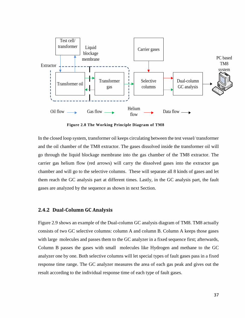


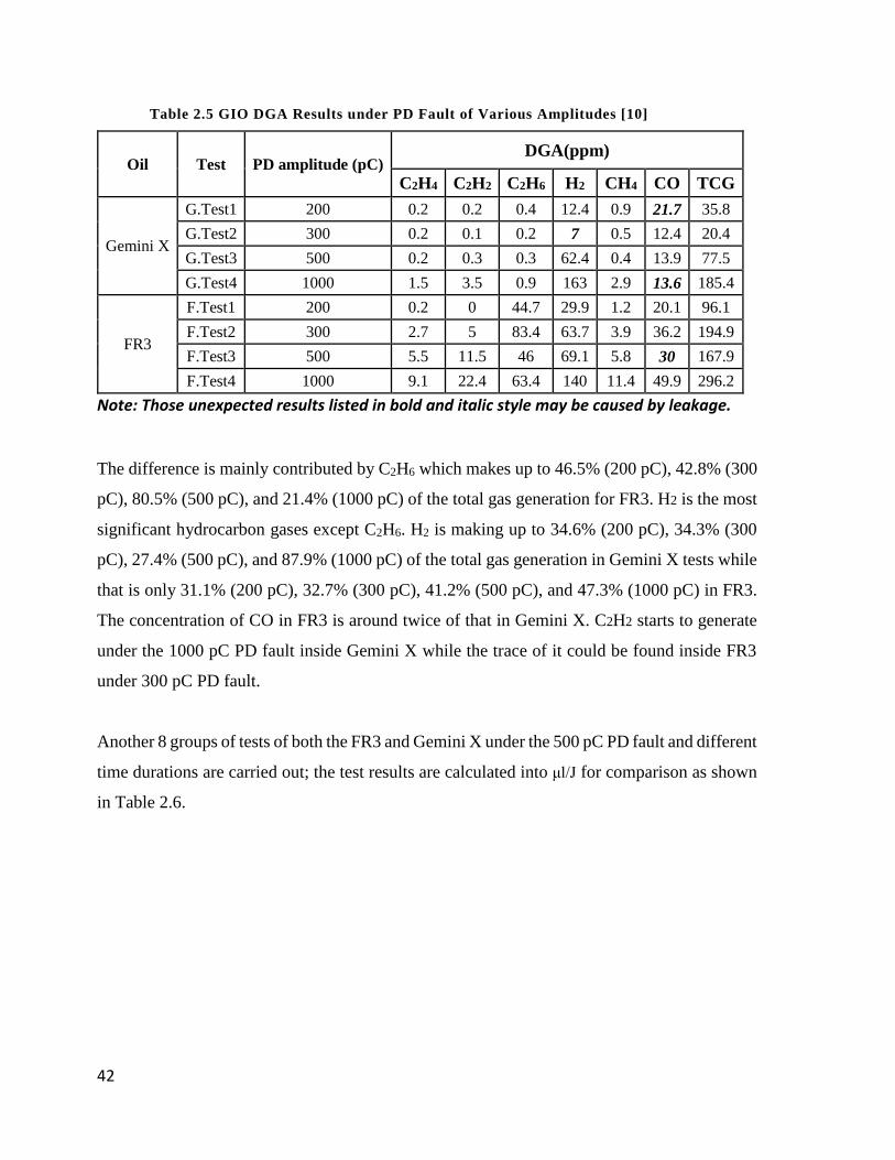
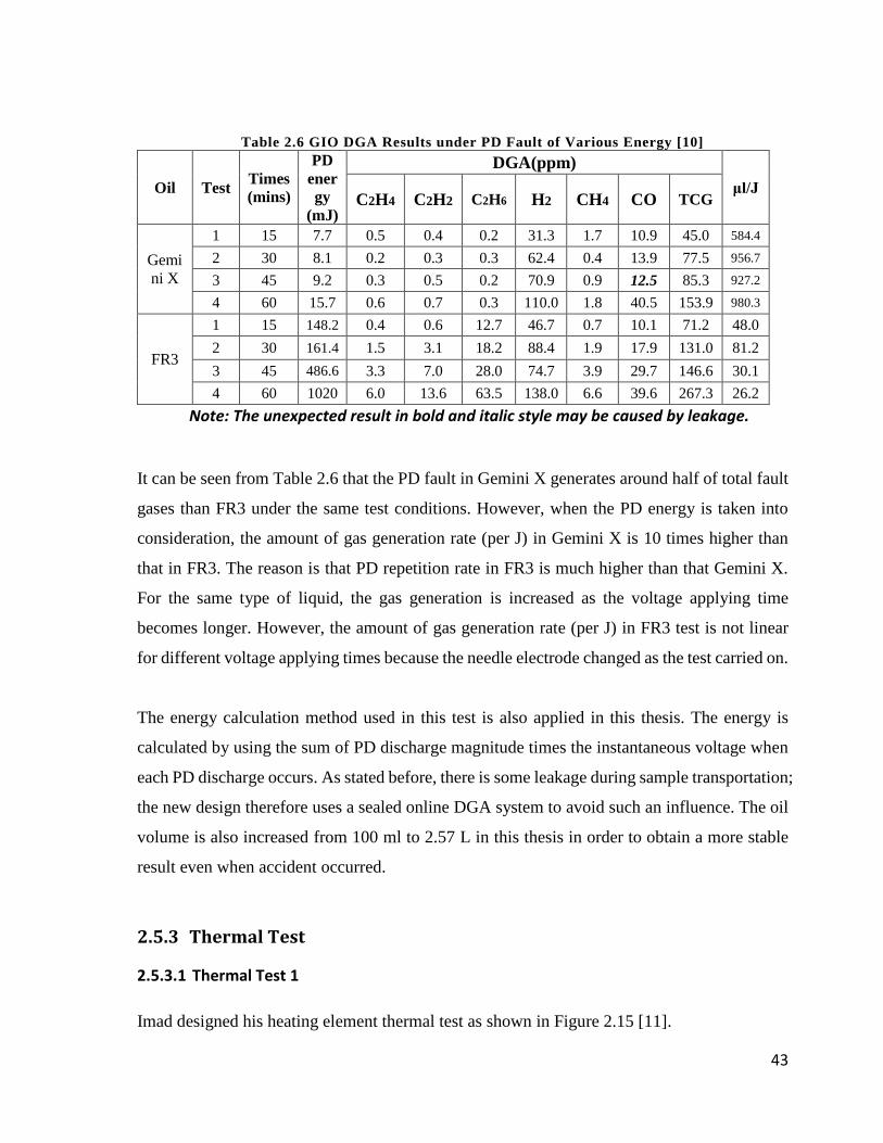
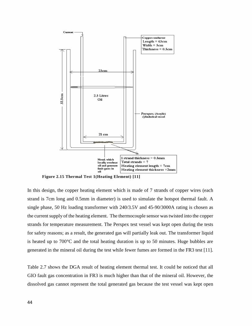
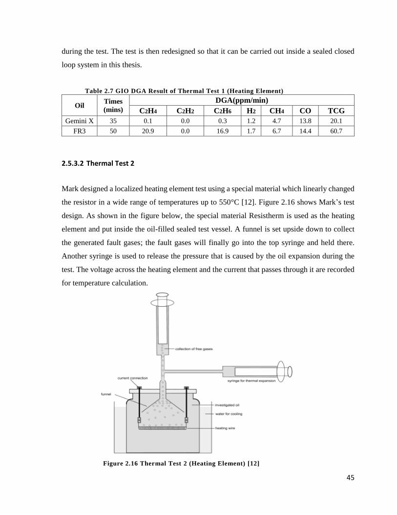


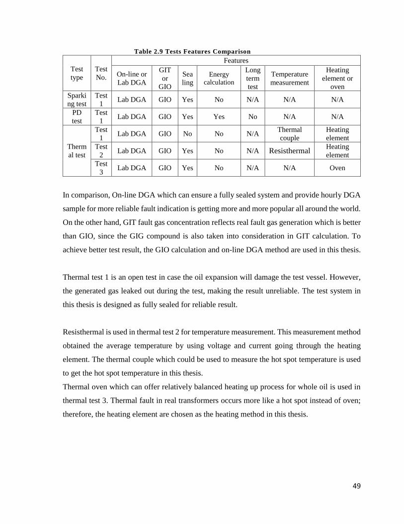

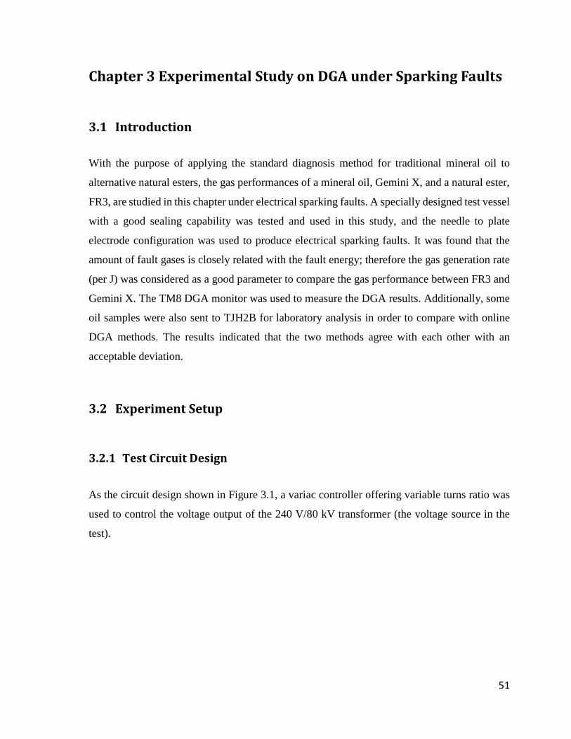
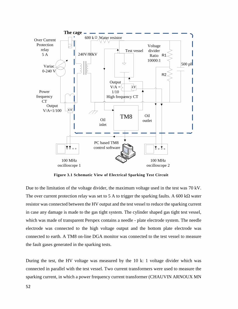
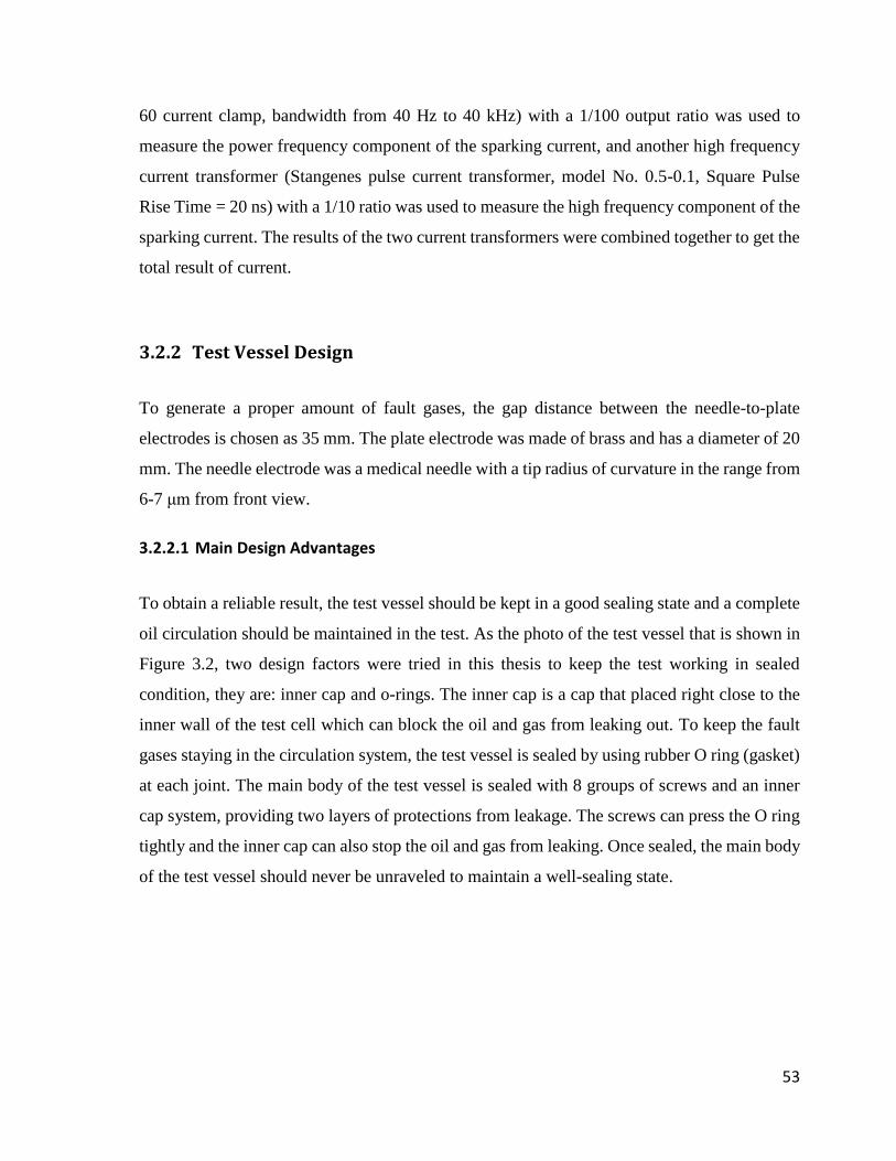


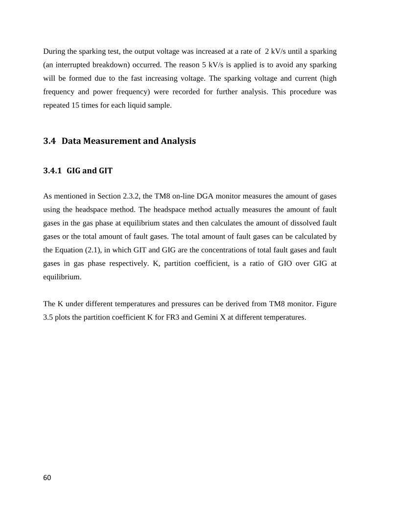


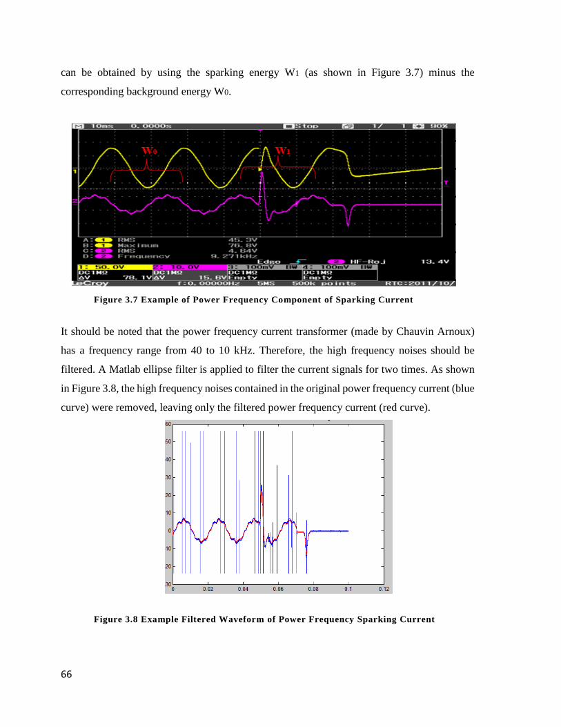
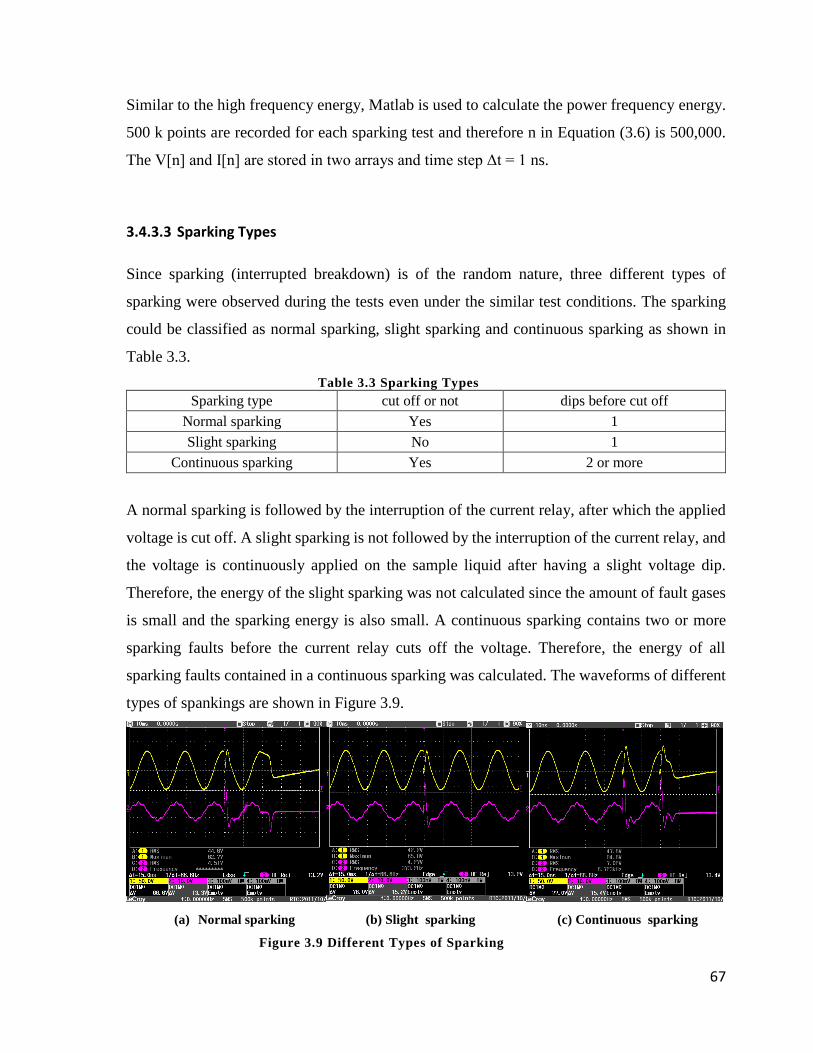


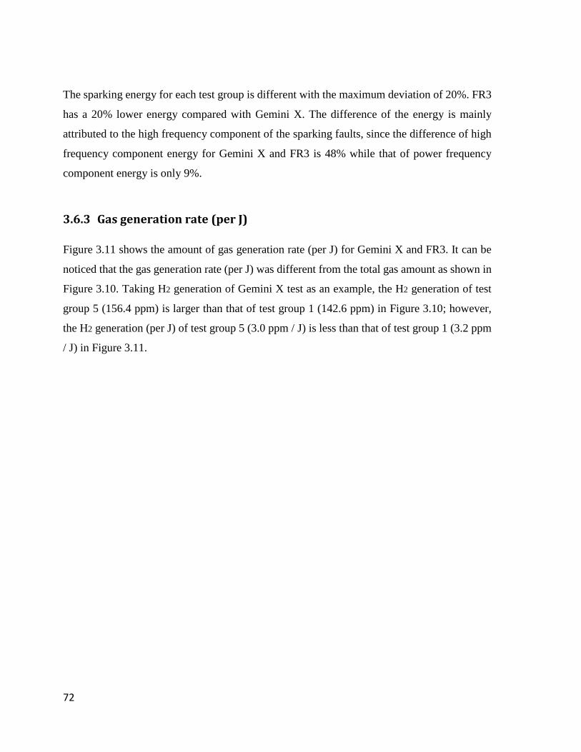


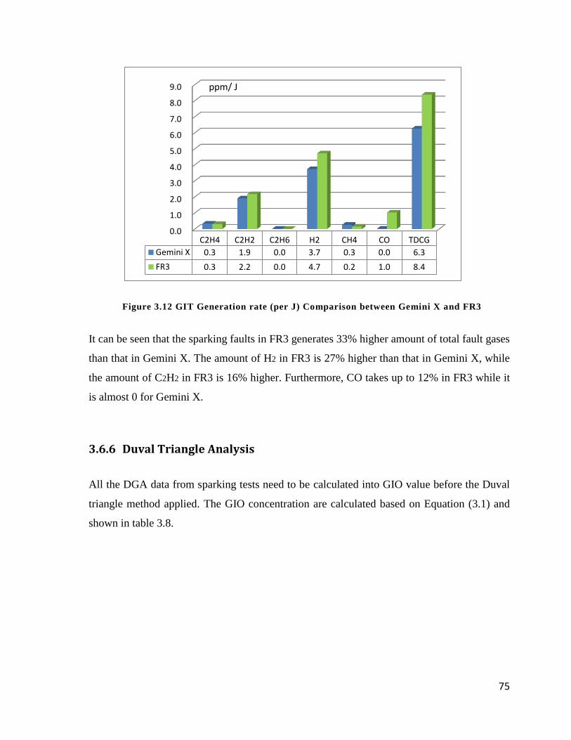


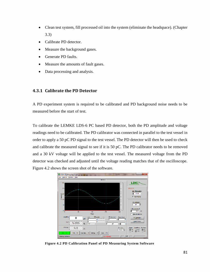


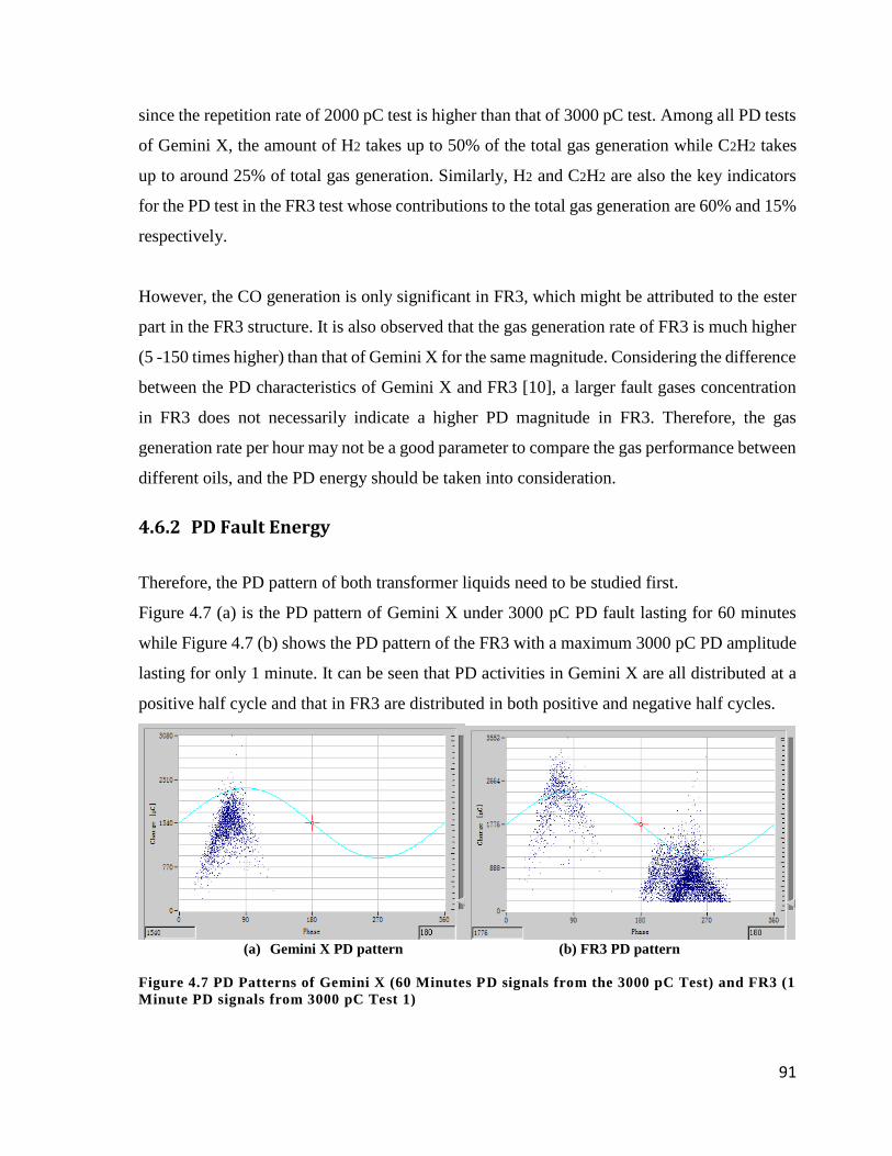
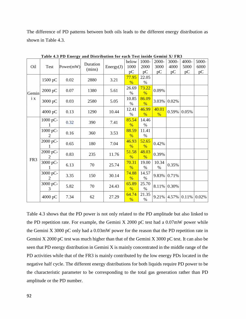
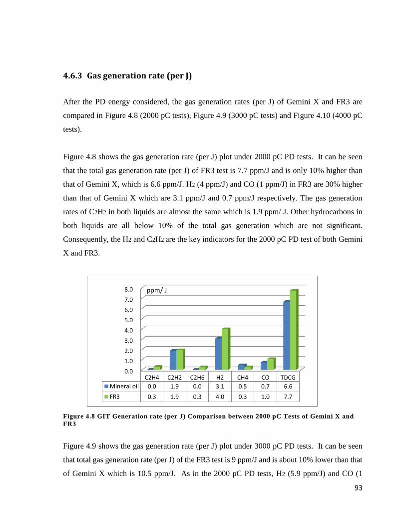

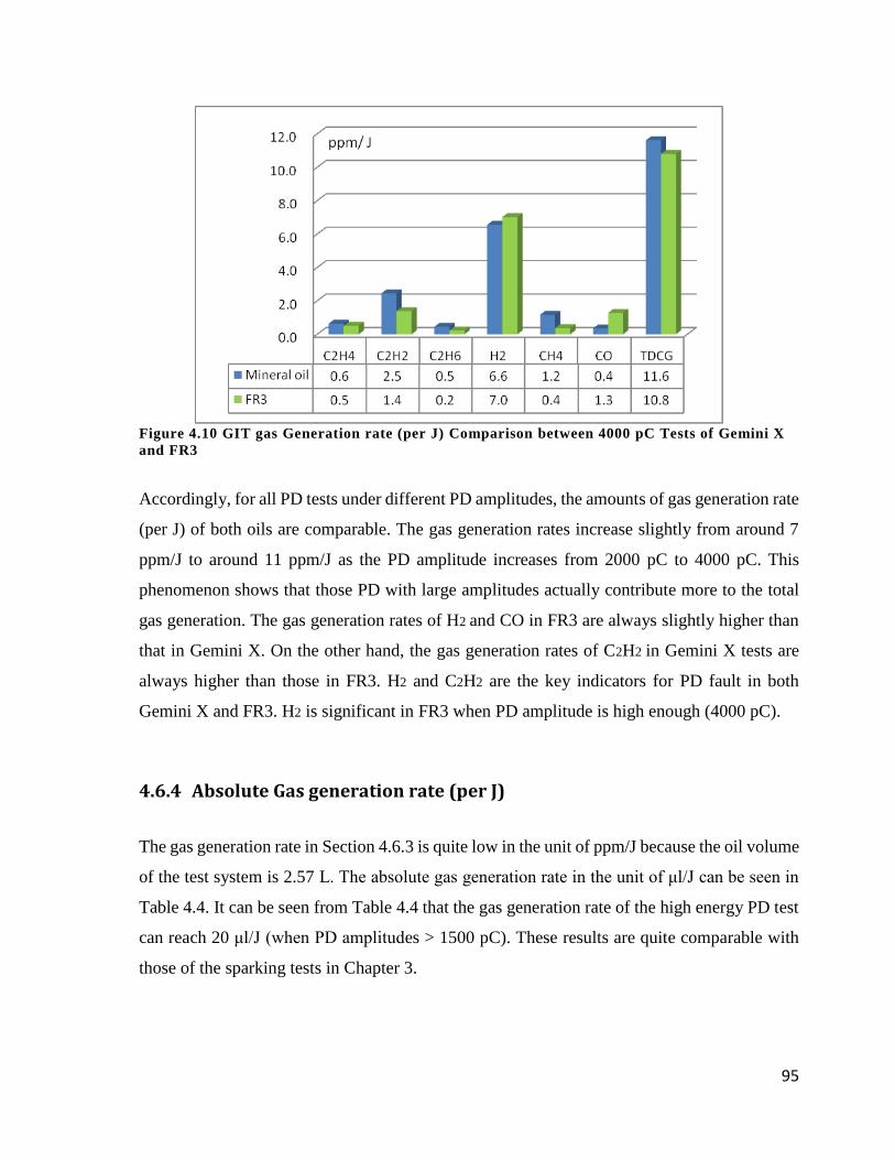


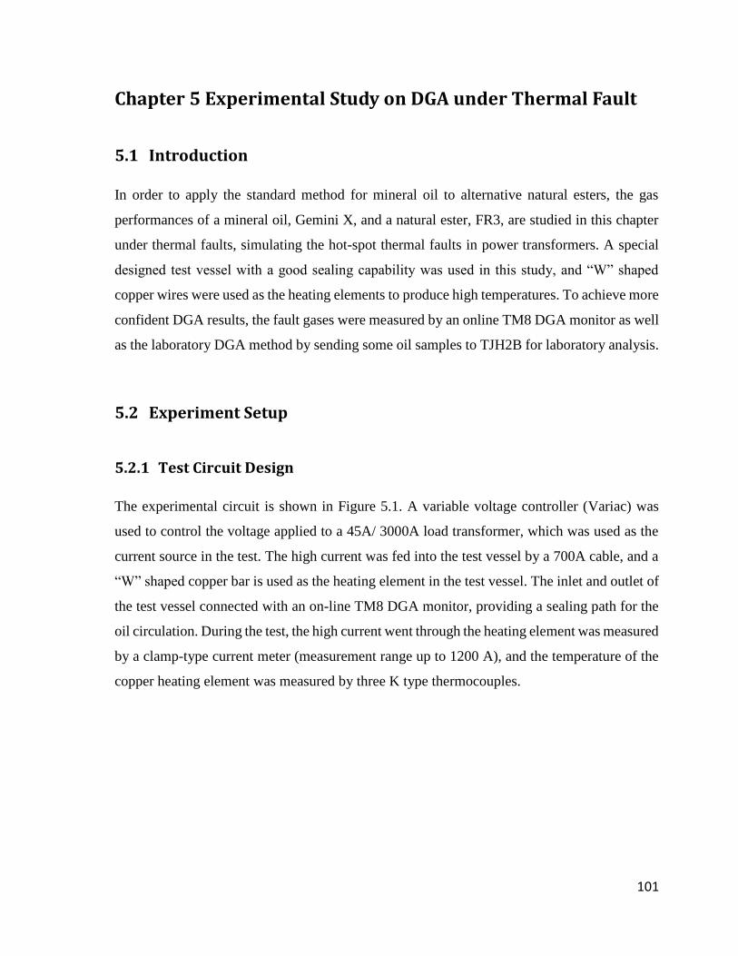
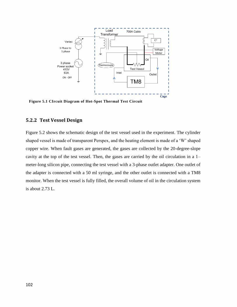


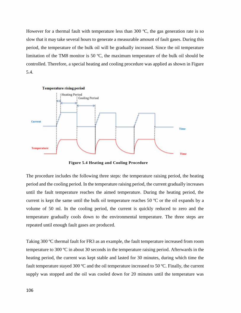
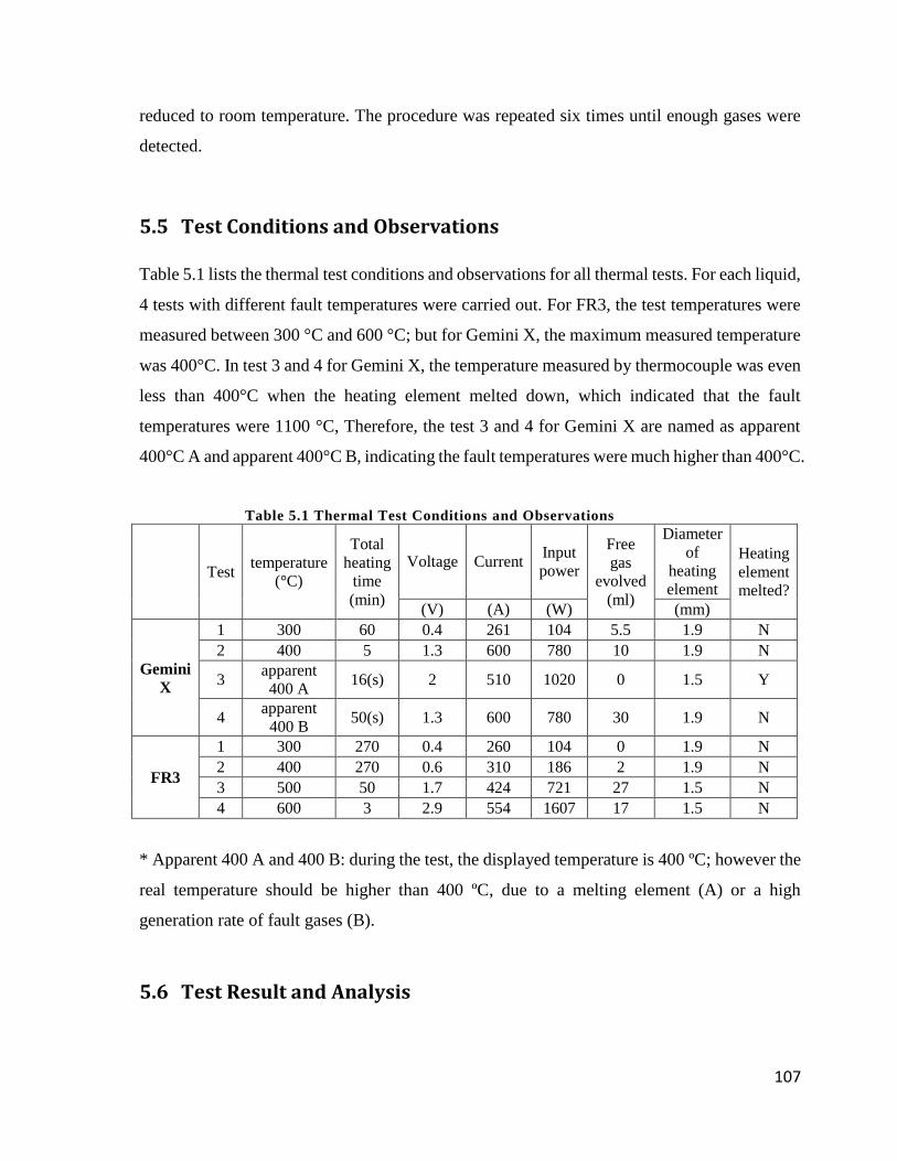


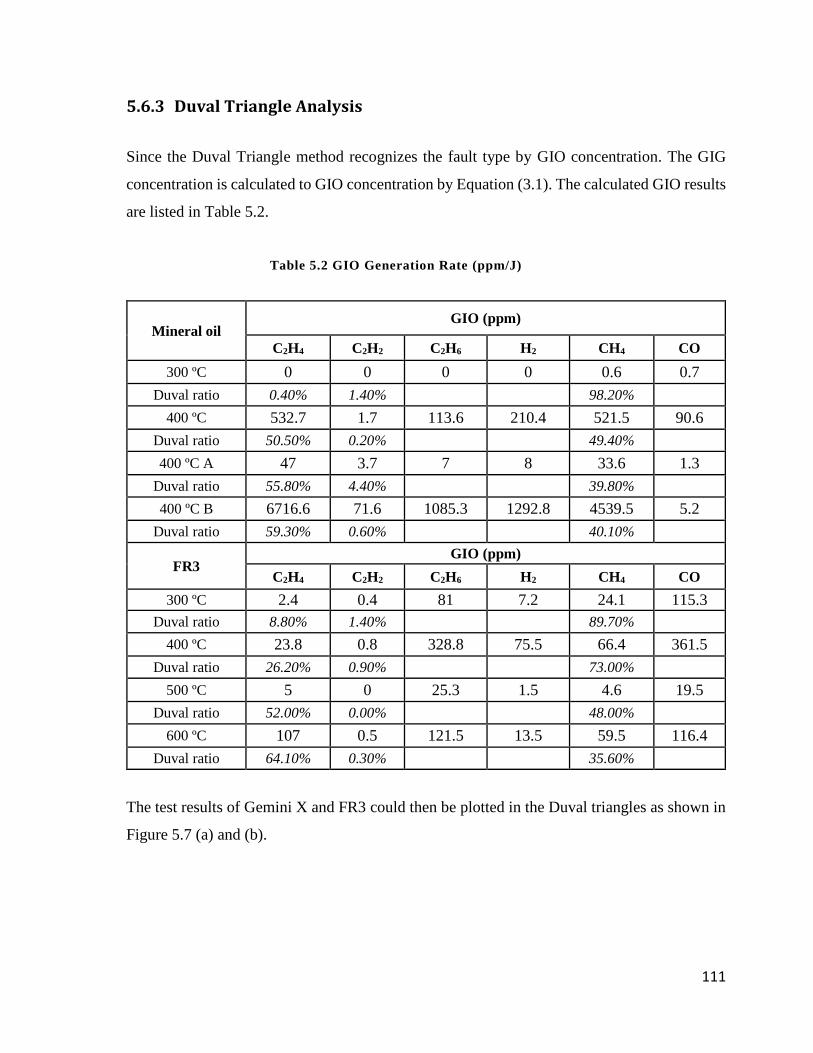
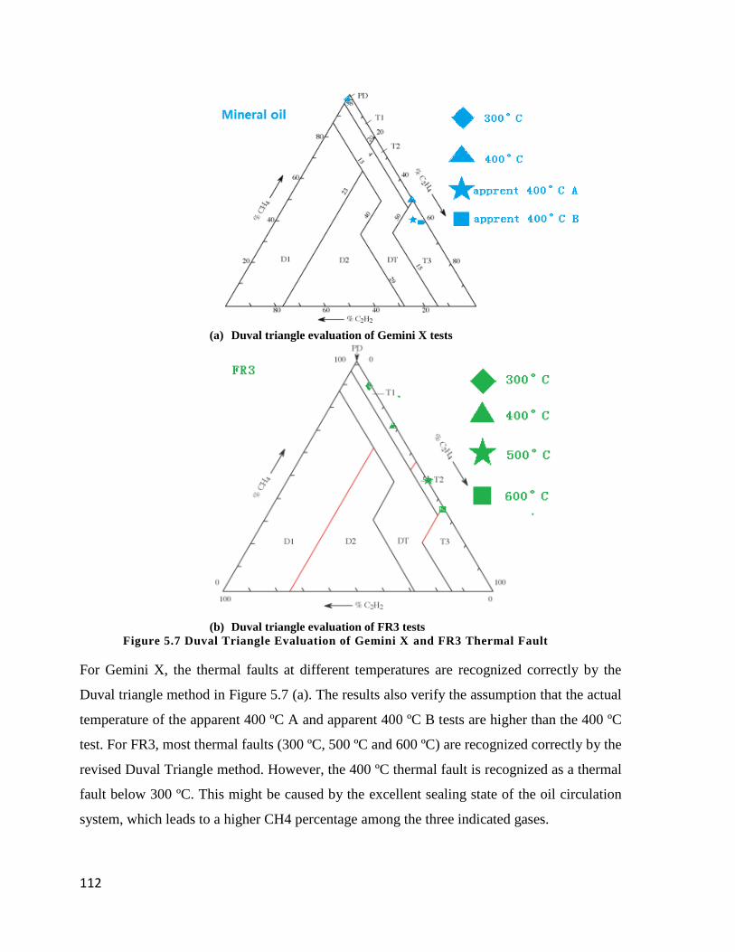
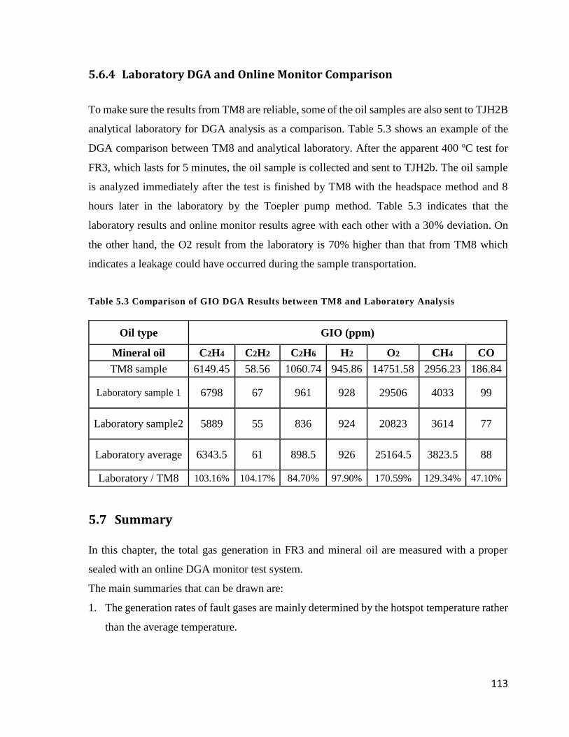


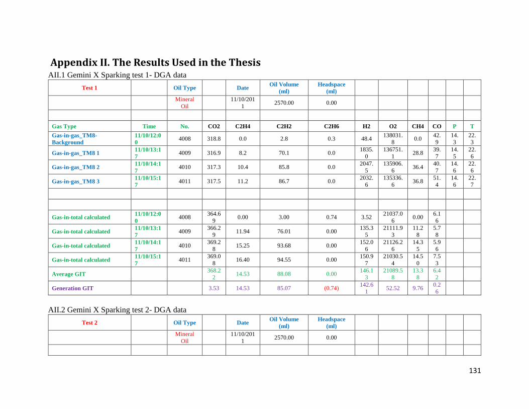
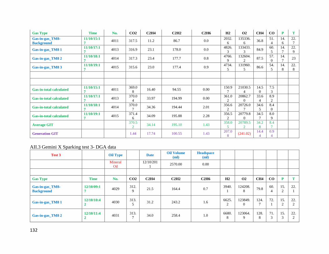


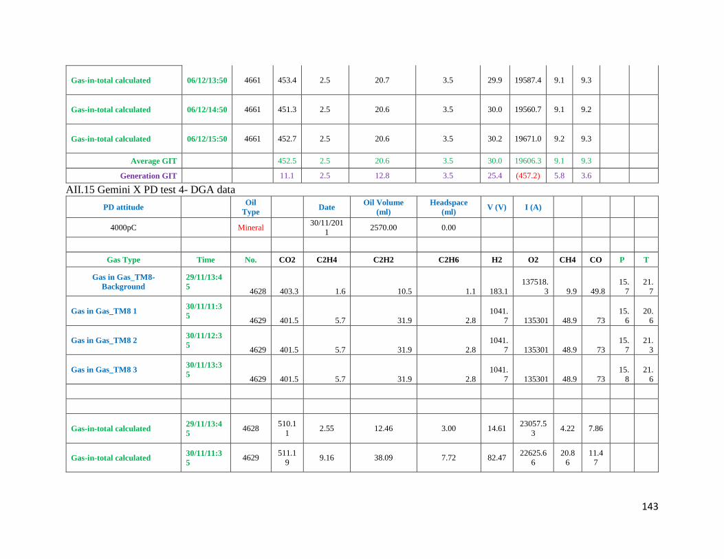

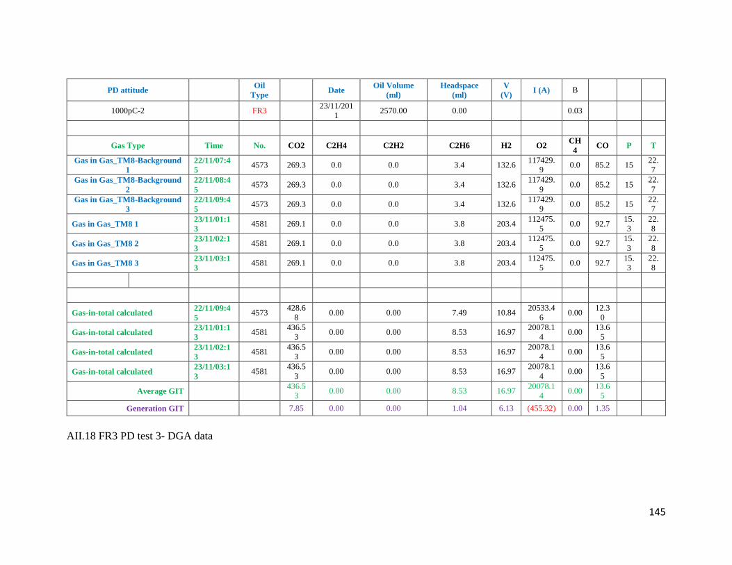

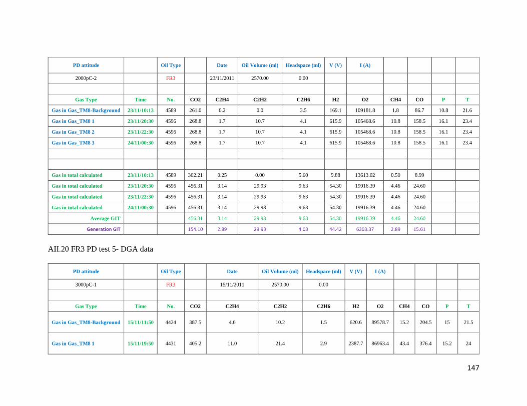


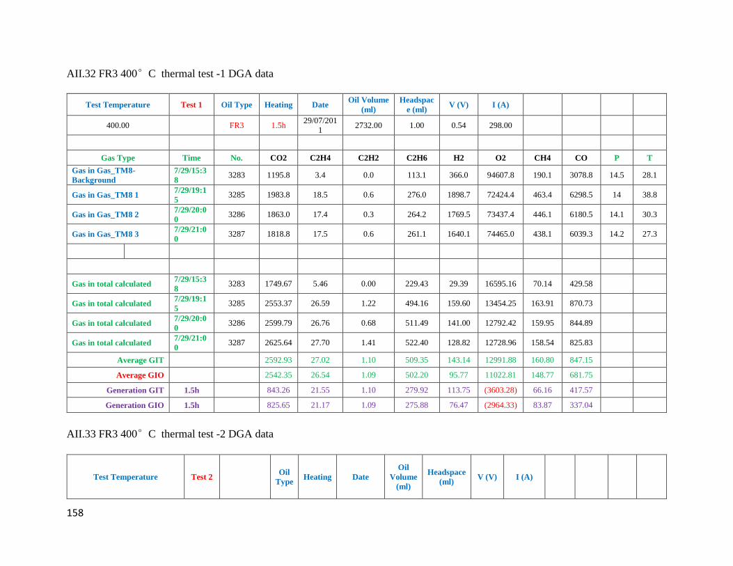

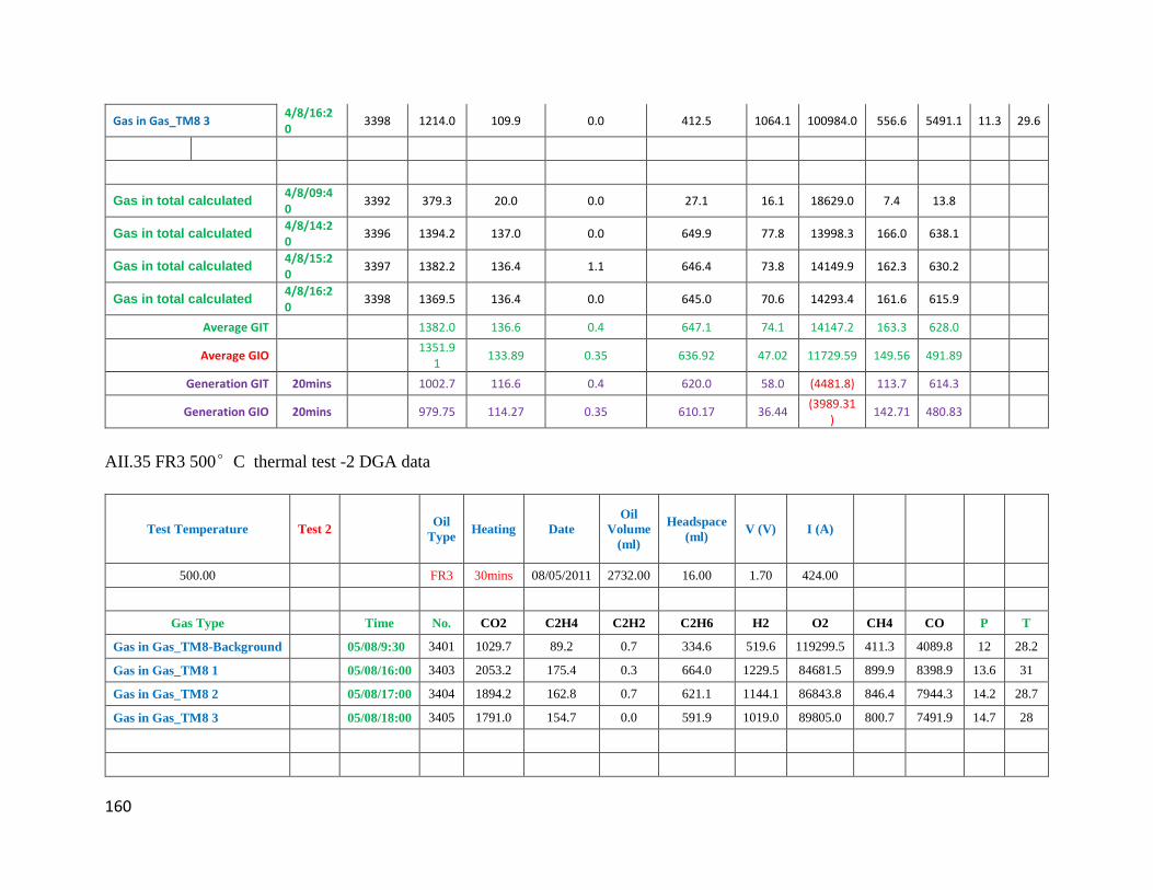

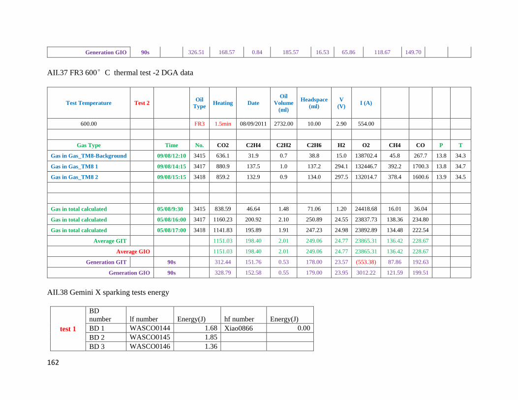


![Power Transformer Dissolved Gas Analysis through Bayesian ... · transformer insulation health assessment through dissolved gas analysis (DGA) [5]. Operational and fault events in](https://static.documents.pub/doc/80x56/5e80fdf1f9cd38246a009341/power-transformer-dissolved-gas-analysis-through-bayesian-transformer-insulation.jpg)


![Dissolved Gas Flotation – Bubble Benefits.ppt Gas.pdfTitle Microsoft PowerPoint - Dissolved Gas Flotation – Bubble Benefits.ppt [Compatibility Mode] Author Ghanim Created Date](https://static.documents.pub/doc/80x56/5e36a195a6c1c809f93fe375/dissolved-gas-flotation-a-bubble-gaspdf-title-microsoft-powerpoint-dissolved.jpg)


