Study of parameter stability of a lumped hydrologic model...

Study of parameter stability of a lumped hydrologic model

in a context of climatic variability

Helene Niela,*, Jean-Emmanuel Paturelb, Eric Servata

aIRD–UMR HSM, BP 64501, 34394 Montpellier Cedex 5, FrancebIRD–UMR HSM, 01 BP 182, Ouagadougou 01, Burkina Faso

Received 6 June 2002; accepted 14 April 2003

Abstract

Central and West Africa were affected by an often marked reduction in rainfall and runoff around the year 1970. Has the

behaviour of the catchments in these regions been changed as a result? Seventeen basins are used in this study, and are

characterised by stationary or non-stationary annual rainfall or runoff time-series. An approach based on lumped hydrological

modelling with a monthly time step (GR2M water balance model) and automatic parameter calibration is used to try to answer

the question. Parameter stability of the models calibrated before and after the occurrence of possible rainfall or runoff deficit is

analysed using estimations of confidence region. Minimisation of the least squares objective function provides a local optimum

around which confidence regions are estimated in a non-linear context. The volumes of indifference represented by the

confidence regions are analysed by their cross-sections on the planes defined by the three parameters of the model taken in pairs.

For each basin, the cross-sections relative to different periods of calibration are interpreted in terms of possible parameter

stability. This study shows that there is no link between parameter stability and the stationary behaviour of rainfall or runoff

series of some catchments.

q 2003 Elsevier Science B.V. All rights reserved.

Keywords: Hydrologic model; Parameter stability; Confidence region; Climatic variability

1. Introduction

The ICCARE program (Identification and con-

sequences of climatic variability in non-Sahelian

West Africa) that is being carried out within the

framework of the FRIEND-AOC project (UNESCO’s

PHI) has resulted in the identification of a climatic

fluctuation in Central and West Africa that appeared

at the beginning of the 1970s (Paturel et al., 1995; Aka

et al., 1996; Paturel et al., 1997; Servat et al., 1997;

Paturel et al., 1998; Servat et al., 1999). The results

generally show a marked reduction in rainfall and

runoff in Central and West Africa. The question that

thus arises concerns the repercussions of average

rainfall and runoff changes on the hydrologic

behaviour of catchments. What is the effect on the

stability of basin behaviour in this type of climatic

variability? To answer this question, drawing on

available hydrologic information concerning

the basins of this region of Africa, we first used

0022-1694/03/$ - see front matter q 2003 Elsevier Science B.V. All rights reserved.

doi:10.1016/S0022-1694(03)00158-6

Journal of Hydrology 278 (2003) 213–230

www.elsevier.com/locate/jhydrol

* Corresponding author. Fax: þ33-4-67-14-47-74.

E-mail addresses: [email protected]

(H. Niel), [email protected] (J.-E. Paturel),

[email protected] (E. Servat).

http://www.elsevier.com/locate/jhydrol

a conceptual rainfall–runoff model to characterise the

main features of the hydrological behaviour of a

catchment, and then a statistical method to assess the

stability of this behaviour through the analysis of the

stability of the parameters of the chosen model. We

had no preconceived idea of what our results would

be. This paper also discusses the relevance of the

approach used.

2. Model and basin hydrological characteristics

2.1. Model used

A lumped water balance model with monthly

inputs was chosen for this study: the GR2M

(Makhlouf and Michel, 1994). This model simulates

monthly discharge using estimations of average

rainfall in a basin. It provides a simplified represen-

tation of the rainfall–discharge process and is

characterised by a small number of parameters

which do not correspond to specific physical attri-

butes. Some of the parameters do, however, contribute

to an equation that allows representation of a

particular process (i.e. evapotranspiration, slow run-

off, etc.). Adjustment of the model’s parameters is

made using a numerical process based on minimis-

ation of criteria, in this case, the method of least

squares. It was the availability of data that guided the

choice of which model to use. It was consequently not

possible to use algorithms that would have allowed

more precise physical modelling of the mechanisms in

play, even if a physical model would have been more

suitable for analysing the variability of the rainfall–

runoff relationship.

The GR2M model (Fig. 1) was developed at

CEMAGREF (Kabouya, 1990). It has been used with

good results in the savannah, forest and transition

regions of Cote d’Ivoire as part of the ERREAU

program (Servat, 1993). This model can be used for

basins of from several hundred km2 to a few thousand

km2, and its main advantage lies in its simplicity. The

following description of the model is from Makhlouf

and Michel (1994):

† a ground reservoir denoted H controls the pro-

duction function and is characterised by its

maximum capacity A;

† a gravity drainage reservoir S controls the transfer

function.

The monthly rain ðPÞ and evapotranspiration (ETP)

are ‘adjusted’ in the same proportion by multiplying

their values by a parameter X1 so that P0 ¼ X1P and

ETP0 ¼ X1ETP: A quantity U which takes the form

U ¼P0ETP0

ðffiffiffiP0

pþ

ffiffiffiffiffiffiETP0

pÞ2

is subtracted from P0 and ETP0 to define Pn ¼ P0 2 U

and En ¼ ETP0 2 U: These last two quantities

condition the dynamics of the reservoir H: If H0 is

the level of the ground reservoir at the beginning of

the time step, H receives a part of Pn and attains the

level

H1 ¼H0 þ AV

1 þH0V

A

with V ¼ tanhPn

A

� �:

Under the effect of En; level H1 of the reservoir H

becomes

H2 ¼H1ð1 2 WÞ

1 þ W 1 2H1

A

� � with W ¼ tanhEn

A

� �:

Fig. 1. GR2M model.

H. Niel et al. / Journal of Hydrology 278 (2003) 213–230214

Pe being the complement of Pn defined by the

equation Pe ¼ Pn 2 ðH1 2 H0Þ; a part of Pe; aPe

flows directly (partition parameter a) while the rest

flows into the gravity drainage reservoir S which

attains the level S1: The discharge from this reservoir

is defined through a parameter X2 so that Qg ¼ X2S1:

Total flow then, is Q ¼ Qg þ aPe:

Makhlouf and Michel (1994) used this version of

the model with good results for 91 French basins,

using the value of 200 mm for A (capacity of the

ground reservoir) and that of 0.2 for the partition

parameter a; X1 and X2 being the only optimised

parameters. Nonetheless, Makhlouf and Michel

(1994) pointed out that, in climatic and physiogra-

phical conditions different from France, A and a

should not be fixed to the above constants, and that it

would be better to optimise them as well. To be

clearer we must specify that X1 was added to the first

version of the model by the authors to reduce the too

large variance of A when this capacity was optimised

for each of the 91 French catchments. The capacity A

was set to 200 mm and the parameter X1 was used to

adjust both P and ETP fluxes rather than to optimise a

proper soil moisture capacity relative to each catch-

ment. The authors specified that their purposes were

pragmatic and not physically based. In the African

context, with an optimisation of A; we decided to keep

parameter X1 but to limit it within the range [0, 1] so

that it could be used as a kind of areal reduction factor.

It could be interesting to test the relevance of using

two distinct parameters to ‘adjust’ P and ETP, but it

was not the purpose of the study presented here.

2.2. Hydrological characteristics

2.2.1. Basins

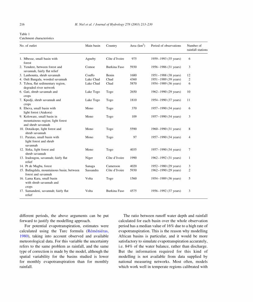
Table 1 lists some characteristics of the basins

chosen for this study. The choice initially concerned

21 basins with surface areas of less than 6000 km2, for

which the data was judged to be sufficient and of good

quality. Only 17 basins were finally used with the

methodology adopted; the four others did not lend

themselves to satisfactory modelling for a parameter

stability study. Note the presence of some small

basins located in the hilly regions of Togo. The basins

are distributed as a function of the different degrees of

reduction in rainfall and runoff:

† in Central Africa, few changes were observed in

Cameroon, but a significant decrease was observed

in Chad,

† in West Africa, few changes were observed in

Benin and Togo, but a notable decrease was

observed in Burkina Faso and in some regions of

Cote d’Ivoire.

Even if they represent different hydrological

conditions in the study area, these basins were not

sufficient to cover the entire region neither do they

lend themselves to regional interpretation.

2.2.2. Data

The available rainfall and discharge data covers

periods of between 30 and 40 years for the majority of

basins studied. Data does not start before the 1950s

and generally stops sometime in the early 1990s. Data

from national networks had to be used for this study

both for discharge and rainfall because the basins are

not used for experimental purposes and consequently

do not have the necessary equipment.

The average rainfall of each basin was calculated

from data from measuring stations located in the basin

and within a 100 km radius using a kriging process. In

this part of Africa, the density of rainfall stations is

very low, and the number of stations used to estimate

average rainfall is consequently too small. Table 1

gives the number of measuring stations involved in

the average rainfall estimate for each basin. Inputs to

the model are characterised by a significant uncer-

tainty, but an attempt was made to compensate for

this. The chosen model allows inputs to be ‘adjusted’

by a multiplicative parameter X1 which partly acts as a

correction factor. Moreover Andreassian et al. (2001)

argue that even if the efficiency of the hydrological

model improves with a better description of watershed

rainfall input, the GR3J model—which belongs to the

same family of models as the GR2M model—in

particular has ‘the capacity to adapt to problems of

rainfall input estimates’. These authors comment on

modelling with a Nash and Sutcliffe criterion reaching

81% for a 10,700 km2 watershed with input from a

single rain gauge, saying that “such good results are

evidence of the fitting properties of rainfall–runoff

models”. In our case, where calibrations of the same

model with the same rain gauges are compared over

H. Niel et al. / Journal of Hydrology 278 (2003) 213–230 215

different periods, the above arguments can be put

forward to justify the modelling approach.

For potential evapotranspiration, estimates were

calculated using the Turc formula (Remenieras,

1980), taking into account observed and available

meteorological data. For this variable the uncertainty

refers to the same problem as rainfall, and the same

type of correction is made by the model, although the

spatial variability for the basins studied is lower

for monthly evapotranspiration than for monthly

rainfall.

The ratio between runoff water depth and rainfall

calculated for each basin over the whole observation

period has a median value of 16% due to a high rate of

evapotranspiration. This is the reason why modelling

African basins is particular, and it would be more

satisfactory to simulate evapotranspiration accurately,

i.e. 84% of the water balance, rather than discharge.

But the information required for this kind of

modelling is not available from data supplied by

national measuring networks. Most often, models

which work well in temperate regions calibrated with

Table 1

Catchment characteristics

No. of outlet Main basin Country Area (km2) Period of observations Number of

rainfall stations

1. Mbesse, small basin with

forest

Agneby Cote d’Ivoire 975 1959–1993 (35 years) 6

2. Yendere, between forest and

savannah, fairly flat relief

Comoe Burkina Faso 5930 1956–1986 (31 years) 3

3. Lanhounta, shrub savannah Couffo Benin 1680 1951–1988 (38 years) 12

4. Ouli Bangala, wooded savannah Lake Chad Chad 4360 1951–1989 (39 years) 2

5. Tchoa, flat sedimentary region,

degraded river network

Lake Chad Chad 5870 1954–1989 (36 years) 6

6. Gati, shrub savannah and

crops

Lake Togo Togo 2650 1962–1990 (29 years) 10

7. Kpedji, shrub savannah and

crops

Lake Togo Togo 1810 1954–1990 (37 years) 11

8. Ebeva, small basin with

light forest (Atakora)

Mono Togo 370 1957–1990 (34 years) 6

9. Koloware, small basin in

mountainous region; light forest

and shrub savannah

Mono Togo 109 1957–1990 (34 years) 3

10. Dotaikope, light forest and

shrub savannah

Mono Togo 5590 1960–1990 (31 years) 8

11. Paratao, small basin with

light forest and shrub

savannah

Mono Togo 97 1957–1990 (34 years) 4

12. Sirka, light forest and

shrub savannah

Mono Togo 4035 1957–1990 (34 years) 7

13. Iradougou, savannah; fairly flat

relief

Niger Cote d’Ivoire 1990 1962–1992 (31 years) 1

14. Pt de Magba, forest Sanaga Cameroon 4020 1952–1980 (29 years) 3

15. Bafingdala, mountainous basin; between

forest and savannah

Sassandra Cote d’Ivoire 5930 1962–1990 (29 years) 2

16. Lama Kara, small basin

with shrub savannah and

crops

Volta Togo 1560 1954–1989 (36 years) 5

17. Samandeni, savannah; fairly flat

relief

Volta Burkina Faso 4575 1956–1992 (37 years) 3


discharge values, are applied to basins in different

climatic and geographical regions, and are able to

provide very good results (Vandewiele and Ni-Lar-

Win, 1998).

2.2.3. Stationarity analyses

For the 17 basins observed, time-series stationarity

analyses were performed for rain, discharge and

runoff coefficient series defined annually. The time-

series of runoff coefficients, i.e. annual runoff water

depth over annual rainfall is interesting because the

variability of this ratio gives an overview of the

behaviour of the annual water balance over time.

The Pettitt test (Pettitt, 1979) shows the possible

abrupt shifts in one and/or the other of the series

(Table 2) in accordance with the results of the

ICCARE program mentioned above. Though a

general coherence can be observed between identified

break dates both for the rainfall and runoff series and

for the runoff coefficients, in some cases there are

significant differences. However, we may recall that

the Pettitt test detects the main break in a series, and if

secondary breaks exist, they are not specified. The

different estimations of the break dates were noted so

that the observation period for each basin could be

divided into two or three sub-periods. The basins for

which no break was detected, regardless of the time-

series analysed (rainfall, discharge or runoff coeffi-

cient) are located in the southern half of Togo and in

the eastern part of the central region. Still, it should be

pointed out that earlier studies have confirmed a

decrease, though slight, in the country’s rainfall

(Paturel et al., 1997), but it is likely that the Pettitt

test is not powerful enough to detect it (Lubes-Niel

et al., 1998). Nevertheless in comparison with the

other basins it is reasonable to assume that the annual

time-series of these basins are not affected by a really

significant abrupt change.

Insofar as all the basins studied are almost

completely natural and have undergone few, if any

changes in terms of land use, it would seem

reasonable to suppose that models of basins for

which the rainfall and discharge time-series are

stationary would exhibit stable parameters over

different calibration periods. Still, a word of caution

about this hypothesis is in order: the stationarity test

concerns series of annual averages whereas the GR2M

model uses monthly data. Stationarity retained for

annual variables does not necessarily imply stationar-

ity for monthly time-series.

Table 2

Break in annual rainfall, runoff and runoff coefficient series (Pettitt test, level of significance 10%)

Basin Rainfall Runoff Runoff coefficient Decision

Break date Deficit (%) Break date Deficit (%) Break date Break retained

1. Mbesse 1976 226 1976 260 1976 1976

2. Yendere 1970 213 1970 257 1971 1970

3. Lanhounta 1963 221 1963

4. Ouli Bangala 1982 224 1970 232 1971 1970 and 1982

5. Tchoa 1970 213 1970 237 1971 1970

6. Gati

7. Kpedji

8. Ebeva

9. Koloware 1981 266 1970 1970 and 1981

10. Dotaikope 1980 215 1970 242 1970 1970 and 1980

11. Paratao 1980 216 1970 241 1971 1970 and 1980

12. Sirka

13. Iradougou 1982 218 1971 245 1971 1971 and 1982

14. Pont de Magba 1969 225 1973 1971

15. Bafingdala 1969 215 1969 228 1969

16. Lama Kara 1980 216 1980

17. Samandeni 1970 216 1970 256 1971 1970


The present study analyses variations in GR2M

model parameters between various periods for each

basin in order to determine the stability of these

parameters; it attempts to interpret this stability from a

hydrological point of view. The Togo basins, qualified

for the sake of simplicity as ‘stationary series basins’,

will be the reference basins with respect to the

adopted approach.

3. Methodology

The methodology used involves two essential steps

for each basin. The first is calibration and validation of

the GR2M model for each period considered. The

second concerns the stability of optimised parameters.

3.1. Model calibration and validation

3.1.1. Preliminary conditions

Each basin is characterised by one or two break

years deduced from the annual series stationarity

study. These years separate the observation periods.

With reference to Paturel et al. (1997), who identified

a decrease in rainfall in Togo around the year 1970,

two modelling periods have been defined for the

‘stationary series basins’, one before 1970 and one

after. The two years on either side of each break year

have been excluded from all calibration. This leads us

to consider a period of 5 years as a transition phase

between two stationary conditions, given that the

break tests (like the Pettitt test) find break points in

simulated series with a margin of error of the order of

2–3 years (Lubes-Niel et al., 1998). For the periods

before and after each transition phase, calibration is

for 75% of the period assumed to be stationary;

validation is reserved for the last 25%. Fig. 2 sums up

the various phases that have been defined for each

basin.

The conditions that were in effect for calibration

are specified below. The parameters to optimise do

not all have the same significance. X1 and a are non-

dimensional constants with values between 0 and 1.

The order of magnitude of X2 is around 1. A is a

capacity, thus a dimensional quantity, expressed in the

same units as precipitation. Bates (1990) recommends

using parameter transformation, which improves the

speed of optimisation convergence and even, in some

configurations, leads to better estimations in the

(inferential) statistical sense of the term. Thus, in

order that all parameters be expressed in the same

order of magnitude, (Vandewiele et al., 1993), the

parameter A was replaced by 1000A0; where A0 is the

new parameter to optimise between 0 and 1.5.

The four parameters of the model were optimised

automatically using the Newton method with least

squares minimisation (Dennis and Schnabel, 1996).

This is a local optimisation method whose drawback,

like all methods of this type, is convergence to a local

optimum (Perrin, 2000). It is therefore advisable to try

to minimise this risk by initialising the algorithm from

different starting points. Thus for each calibration, the

domain of variation for each parameter was discre-

tised. The optimisation algorithm was implemented,

using for initial values each node of this grid

corresponding to a quadruplet ðA0;X1;X2;aÞ: The

procedure converged in almost every case towards the

same minimum, except for some sets of quadruplets

which had, as an initial value for a limited parameter,

X1 or a; a theoretical limit (1 for example). Then the

objective function value after optimisation was

greater than that obtained from the other initial points.

After the calibrations were done, it turned out that for

16 basins, parameter a was equal to 0. Only the

Koloware basin with a surface area of 109 km2, thus

smaller than the others, presented a partition par-

ameter of 0.33 in the first calibration period. So on a

monthly scale, generally no rapid runoff is represented

by the model. The same thing can be observed in

similar types of monthly models of other humid

African catchments (main basin: Sassandra) with

areas in the same order of magnitude (Ardoin, 2002,

pers. comm.), meaning that part of the rain from any

given month cannot be found in the river during the

course of the same month. Is this the real behaviour of

these basins or do the models used fail to correctly

take into account the monthly direct runoff in these

humid regions of Africa? In the end we decided to

simplify the structure of the GR2M model by not

using a variable that represents this runoff but rather

using only one component for runoff, that being the

flow from a storage reservoir provided that good

fitting could be achieved. These results led us to set

the parameter a to 0 (even for the Koloware basin)

and then to make another optimisation run in a

parameter space with a lower dimension.


3.1.2. Modelling results

3.1.2.1. Quality criteria. Nash non-dimensional effi-

ciency criterion values are shown in Fig. 2 to allow

comparisons of model performance between different

periods and different basins. The efficiency criterion

(Nash and Sutcliffe, 1970) is written by

1 2

PðQobsi

2 QcaliÞ2P

ðQobsi2 �QobsÞ

2

Fig. 2. Calibration, validation and transition phases per basin.


with Qobsiand Qcali

; respectively, the monthly

observed and simulated flows and �Qobs the mean

monthly flow. The fit between simulated and observed

discharges is even better because the Nash criterion

expressed as a percentage is near 100%. Nash and

Sutcliffe (1970) point out that there is no objective test

for the significance of their criterion because the

model’s degrees of freedom are not known. Still, as a

practical matter, a criterion less than 60% does not

give a satisfactory fit between observed and simulated

hydrographs, a problem largely due to out of phase

timing.

Using only the Nash criterion to judge adequate

fitting of model simulations with observed data is still

not always sufficient. To this overall index of model

quality we have added the calculation of a relative

absolute mean error denoted ErV between observed

annual flow volumes and those simulated by the

model throughout the calibration period ðNan ¼

yearsÞ :

ErV ¼1

Nan

XNan

i¼1

lVobsi2 Vcali

lVobsi

This index was also calculated for the validation

periods. It is complementary to the Nash criterion

which can be high when the volume error is high. This

index is calculated only for those years when the

observed volume is non-zero. As the variability of peak

discharge can be high for some basins from one year to

the next, this criterion takes into account the agreement

between observation and simulation for small hydro-

graphs, whereas the Nash criterion gives low weight to

these discharges which can be badly simulated.

Considering the unknown measurement precision of

runoff, we have deemed as acceptable relative error in

volume somewhere in the range of 30%. Referring to

Ouedraogo (2001), we observe for the basin of

Bafingdala for the period 1972–1985 that the GR2M

model applied in a spatially distributed version

provides in calibration 89% for the Nash criterion

and 17% for the relative error in volume, instead of,

respectively, 79 and 27% for our lumped version. If we

compare the hydrographs observed and simulated from

the two versions (Fig. 3) we can consider the lumped

simulation as acceptable both for the high discharges

and for the low flows. The same goes for the other

series with respect to a relative error in volume of

around 30%. We were able to observe that only a few

events increase the volume criterion, and that most of

simulated hydrographs are of good quality. It should be

noted that in general in hydrological modelling, only

the Nash criterion is used to assess the fit between

simulated and observed graphs, and even if the limit of

30% for the relative error in volume remains

questionable, here it is a supplementary and objective

guarantee of a model’s reliability.

Fig. 3. Comparison of two kinds of simulations with the GR2M model for the basin of Bafingdala.


3.1.2.2. Actual results. The optimised values obtained

are shown in Table 3. A number of remarks should be

made concerning the results. Some of the values

resulting from optimisation should attract attention

even if the parameters do not represent a specific

physical attribute. For example, during the period

1985–1988, Ouli Bangala shows an optimised value

of A equal to 0. Given the principles of the model, this

means that the best fit of the simulated hydrograph

with observed data can only be made by cancelling the

water stock of the ground reservoir, meaning the

actual evapotranspiration; all the water available

should be used for runoff. In fact, coming back to

the data, it appears that the flood in 1985, the largest in

the four-year calibration sample, composed of one

flood per year, orients the optimisation process

towards the results obtained. The weight of this

flood would not have had the same significance in a

sample such as the first period of 1951–1963, which

was more representative of the annual floods observed

in this basin. The bias introduced in the calibration of

1985–1988 is prejudicial to the analysis of parameter

stability. Thus for this basin, only the first two periods

were retained. Like the other lumped conceptual

models, the GR2M model is able to satisfactorily

simulate events whose main characteristics are

represented in the calibration sample. Otherwise, it

is difficult for the model to produce a good fit for

a particular event which has a low relative weight in

the calibration sample. These models behave like

statistical models as their performances are dependent

on the representativeness of the calibration samples.

A good calibration should translate into a high

Nash criterion value and a low relative error in

volume. In a good model these two conditions should

be observed not only in calibration but also during

validation when the model is applied with data not

used in calibration. Considering these different

conditions, only the following basins are modelled

correctly in terms of the two selected criteria: Ouli

Bangala (no. 4) until 1979, Dotaikope (no. 10) until

1977, Paratao (no. 11) until 1977, Iradougou (no. 13),

Pont de Magba (no. 14) and Lama Kara (no. 16).

Given the small number of basins selected, we

introduced a tolerance factor for the volume criterion

so that the following basins could also be considered:

Yendere (no. 2), Gati (no. 6), Koloware (no. 9) until

1975 and Paratao (no. 11) for the entire observation

period. Finally, the Togo basins, including Kpedji (no.

7), Ebeva (no. 8) and Sirka (no. 12), for which the

Nash criteria were satisfactory, were used by virtue of

their interest as ‘stationary series basins’, despite the

high values of the volume criterion due to bad

simulations of hydrographs showing low discharge

values, and even if the rigour of the processes can be

considered as weakened by this decision. Examples of

Table 3

GR2M parameters optimised

Basin 1st calibration period, X1=X2=A (mm) 2nd calibration period, X1=X2=A (mm) 3rd calibration period, X1=X2=A (mm)

1. Mbesse 1959–1969, 0.44/0.72/136 1979–1989, 0.40/0.82/104

2. Yendere 1956–1964, 1/0.65/564 1973–1982, 0.94/0.69/669

3. Lanhounta 1951–1957, 0.51/0.86/189 1966–1985, 0.56/0.88/228

4. Ouli Bangala 1951–1962, 0.82/0.67/252 1973–1979, 0.55/0.67/145 1985–1988, 0.44/0.42/0

5. Tchoa 1954–1963, 0.56/0.44/552 1973–1987, 0.66/0.40/804

6. Gati 1962–1966, 0.44/0.74/165 1973–1985, 0.39/0.80/154

7. Kpedji 1954–1963, 0.68/0.70/278 1973–1985, 0.59/0.81/278

8. Ebeva 1957–1964, 0.75/0.70/266 1973–1985, 0.65/0.74/332

9. Koloware 1957–1964, 0.90/0.73/306 1973–1975, 0.75/0.64/729 1984–1989, 0.58/0.84/352

10. Dotaikope 1960–1965, 0.75/0.85/354 1973–1976, 0.76/0.73/470 1983–1988, 0.75/0.82/434

11. Paratao 1957–1964, 0.65/0.71/103 1973–1976, 0.92/0.77/974 1983–1988, 1/0.87/1083

12. Sirka 1957–1964, 0.62/0.73/450 1973–1985, 0.55/0.70/319

13. Iradougou 1962–1966, 0.69/0.63/369 1974–1978, 0.53/0.60/269 1985–1990, 0.66/0.61/431

14. Pt de Magba 1952–1964, 1/0.55/457 1974–1978, 1/0.44/43

15. Bafingdala 1962–1965, 0.58/0.47/371 1972–1985, 0.47/0.52/125

16. Lama Kara 1954–1971, 1/0.94/393 1983–1988, 1/0.90/506

17. Samandeni 1956–1964, 1/0.59/1022 1973–1987, 0.46/0.66/272


observed and simulated runoff are presented in Fig. 4

with the values of the corresponding determination

coefficients R2; each period of simulation being

composed by a calibration period and its correspond-

ing validation period. R is the correlation coefficient

between observed and simulated runoff. We can

especially remark the quite acceptable quality of the

simulation for the Kpedji basin which does not satisfy

the volume conditions expressed by the ErV index.

3.2. Analysis of parameter stability

3.2.1. Principle and first general results

about the GR2M model

The proposed stability analysis is based above all on

analysis of the sensitivity of optimised parameters.

According to Sorooshian and Gupta (1995), this

consists of estimating the ‘region of indifference’ for

the calibrated parameters, in other words, “the region

around the best parameter estimates in which the

objective function value varies from the best function

value by only a small indifference value 1”. In this zone

the values generated for the different parameters are

not the optimum values but they do not significantly

damage the fit between simulated and observed

hydrographs. Determining this zone of agreement is

not unique. Thus Sorooshian and Gupta (1995) use

quadratic approximations of the objective function in

the neighbourhood of the optimum. The second

derivatives are evaluated numerically and the defined

zone of agreement describes a hyperellipse in the

parameter space. This approach supposes that the

degree of non-linearity of the model is negligible.

Other approaches rely on variable transformations to

satisfy as best they can the application conditions of

linear models (Bates, 1990). The procedure that we

have selected here identifies the aforementioned zone

of agreement to the confidence region of non-linear

model parameters (Draper and Smith, 1981; Troutman,

1985). The contour of this region is calculated for a

given probability level equal to ð1 2 arÞ such that the

confidence region, thus defined, contains the optimum

and unknown set of parameters u of the model with a

probability approximately (not exactly the same as in a

linear model) equal to ð1 2 arÞ: The value of the

contour of this confidence region, FcðuÞ; depends on

the minimum value of the least squares objective

function Fcopt, and of the Fisher variable F to p and

n 2 p degrees of freedom for a non-exceedance

probability of ð1 2 arÞ with p the number of par-

ameters to optimise and n 2 p the number of

calibration observations minus the number of par-

ameters to optimise:

FcðuÞ ¼ Fcopt1 þ

p

n 2 pFðp; n 2 p; 1 2 arÞ

� �� ð1Þ

In the framework of a similar methodology even if in a

different scientific field, Laloe (1995) reminds us that

in the case of non-linear models, confidence regions

associated with one or several parameters are generally

not symmetrical around the optimum estimates. This

asymmetry can be explained by a distribution of the

parameter estimates that is neither normal nor

symmetrical even if the distribution errors turn out to

be normal.

For each calibration three contours have been

defined by the cross-sections on the planes ‘A 2 X1’

(X2 remaining at its optimum value), ‘A 2 X2’ (X1

remaining at its optimum value), and ‘X1 2 X2’ (A

remaining at its optimum value) of the ‘volume of

indifference A 2 X1 2 X2’ estimated around the

optimum by using expression (1) with a confidence

level of 95 and 99%. Figs. 5a–c, 6a–c, 7a–c and

8a–c represent the contours obtained, respectively, in

the planes ‘A 2 X1’; ‘A 2 X2’; and ‘X1 2 X2’ for the

different calibration periods. For the first two planes,

the figures must be interpreted in terms of ‘A0 2 X1’

and ‘A0 2 X2’; the abscissa caption recalling that A ¼

1000A0: The indices 1, 2 or 3 of the contours

characterise, respectively, the first, second and

possibly the third period of calibration. The geometry

of the contours gives information about the relative

sensitivities of parameters and their interactions.

When the shapes are ellipsoidal, Sorooshian and

Arfi (1982) propose ‘concentricity and interaction’

measures to allow objective comparison of the

influence of various objective function formulations

on the relative behaviour of parameters. The qualitat-

ive interpretation of contours relative to parameters

taken in pairs leads to the following conclusions in

this study. Figs. 5a–8a reveal an interaction between

parameters A0 and X1 since neither of the two axes of

the pseudo-ellipsoidal curves is parallel to any of the

axes of the co-ordinates in the space of the parameters

considered. Moreover, the orientation of the curves

defines a direction whose angle is less than 458 from


Fig. 4. Examples of observed and simulated monthly runoff hydrographs.


Fig. 5. Cross-sections of the parameter confidence volume for the basins no. 2, no. 4 and no. 6. (a) Plane ‘A 2 X1’: (b) Plane ‘A 2 X2’: (c) Plane

‘X1 2 X2’:


Fig. 6. Cross-sections of the parameter confidence volume for the basins no. 7, no. 8 and no. 9. (a) Plane ‘A 2 X1’: (b) Plane ‘A 2 X2’: (c) Plane

‘X1 2 X2’:


Fig. 7. Cross-sections of the parameter confidence volume for the basins no. 10, no. 11 and no. 12. (a) Plane ‘A 2 X1’: (b) Plane ‘A 2 X2’:

(c) Plane ‘X1 2 X2’:


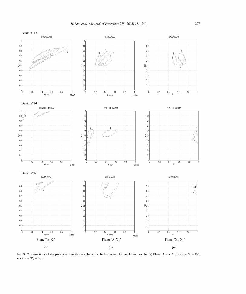
Fig. 8. Cross-sections of the parameter confidence volume for the basins no. 13, no. 14 and no. 16. (a) Plane ‘A 2 X1’: (b) Plane ‘A 2 X2’:

(c) Plane ‘X1 2 X2’:


the A0 axis, meaning that X1 has a greater degree of

sensitivity than A0: Figs. 5b–8b on the other hand,

show that parameters A0 and X2 interact little in

general and that the orientation of their curves, more

or less parallel to the X2 axis, demonstrates a greater

degree of sensitivity of parameter A0 compared to X2:

Finally Figs. 5c–8c show a weak interaction between

X1 and X2; X1 being more sensitive than X2; as

Makhlouf and Michel (1994) have pointed out in

temperate zones.

3.2.2. Analysis of parameter stability per basin

The analysis of stability for each basin is first

oriented towards the interpretation of the cross-

sections of the confidence region on the planes defined

by the parameters taken in pairs, the third parameter

remaining at the optimum value. The confidence

contours described in each plane relative to the two

or three compared calibration periods per basin can be

classified, depending on three possible situations:

† disjunction: contours are disjoint,

† overlap: the contours partly overlap or are only

contiguous,

† inclusion: one of the contours is included in the

other.

In our approach, the conclusion of stability or not

derives from the following interpretation of the above

three situations. First of all we decided to translate an

inclusion configuration into a stability conclusion for

the parameters between the periods concerned. To go

further, we extended this conclusion concerning

stability to cases in which there is overlap of defined

contours and possibly a borderline overlap (contig-

uous configuration). Actually we accept that volumes

that partly overlap refer to a same sub-region of

parameter space, which is a consequence of the fact

that the confidence volumes are only estimators for an

approximate probability level of unknown theoretical

volumes. Conversely disjoint contours preclude the

hypothesis of parameter stability between the different

periods. Obviously the conclusion concerning

stability or not derives from this kind of

interpretation considering the results of the full set

of the three planes of pairs of parameters. The last

column of Table 4 summaries the degree of parameter

stability.

Table 4

Interpretation of the three cross-sections of the parameter confidence volume

Basins ‘Stationary

series basin’:

Yes (Y) or

Not (N)

Plane ‘A0-X1’

contours

Plane ‘A0-X2’

contours

Plane ‘X1 2 X2’

contours

Parameter stability:

Yes (Y) or Not (N)

2-Yendere N Contiguous Overlapping Overlapping Y

4-Ouli Bangala

until 1979

N Disjoint Overlapping Disjoint N

6-Gati Y Overlapping Inclusion Overlapping Y

7-Kpedji Y Overlapping Overlapping Overlapping Y

8-Ebeva Y Contiguous Inclusion Overlapping Y

9-Koloware

until 1975

N Disjoint Disjoint Contiguous N

10-Dotaikope

until 1977

N Overlapping Overlapping Overlapping Y

11-Paratao N First two periods:

disjoint; last two

periods: inclusion

First two periods:

disjoint; last two

periods: overlapping

First two periods:

disjoint; last two

periods: overlapping

First two periods: N;

last two periods: Y

12-Sirka Y Inclusion Overlapping Overlapping Y

13-Iradougou N First two periods:

contiguous; last two

periods: inclusion

First two periods:

overlapping; last two

periods: contiguous

First two periods:

disjoint; last two

periods: disjoint

First two periods: N;

last two periods: N

14-Pont de Magba N Disjoint Disjoint Overlapping N

16-Lama Kara N Overlapping Overlapping Overlapping Y


When the parameter stability is rejected, the

confidence volume cross-sections on the different

planes give some information about the parameter(s)

particularly involved in the decision. For instance, for

Ouli Bangala, Koloware, Paratao (first two periods),

parameters X1 and A especially are involved. For Pont

de Magba only A is particularly involved. For

Iradougou, X1 is concerned; however, the disjunction

is not very pronounced between the last two periods,

and we can reasonably conclude that the full set of

parameters is quasi-stable.

These results concerning stability or not lead to the

conclusion that stability is not simply linked by the

presence or not of a break in the annual time-series of

the basins. For instance, the ‘stationary series basins’

(Gati, Kpedji, Ebeva, Sirka) as well as others

(Yendere, Dotaikope, Paratao, Lama Kara) are

concluded to be stable. Another fact is that all the

‘stationary series basins’ present stable parameters.

However, we must be careful about generalizing this

result as only four such basins were included in this

study.

4. Conclusions

The work presented above was carried out on 17

basins from West and Central Africa. Because

available data comes from national rainfall and

hydrometric networks, the study is rooted in a

conceptual hydrologic modelling context. The meth-

odology consists of comparing for each basin, using a

statistical approach, model parameters estimated by

automatic calibration over different periods and more

especially before and after abrupt shifts detected on

data series most often around 1970. For each basin the

physical characteristics (vegetation, land use, etc.)

remain constant for the duration of observations, and

the rainfall input is estimated from the same rain

gauges for all the calibration or validation periods.

The statistical procedure takes into account the

possible dependencies between parameters and

defines a confidence region in which the parameter

values are not the optimum values but do not

significantly influence the fit between simulated and

observed hydrographs. Cross-sections of this confi-

dence region based on pairs of parameters are

interpreted in terms of stability or not of the GR2M

model parameters. We see from the results that non-

stationarity in rainfall or runoff series does not imply

non-stability of the model parameters. If we accept the

hypothesis that parameter stability can be translated

into hydrologic stability, we can conclude that

climatic variability does not always imply variability

in the hydrologic behaviour of basins. The type of

model used—which belongs to the family of lumped

conceptual models with parameters estimated by

automatic numeric optimisation—can cast doubt on

this hypothesis. The limitations of this kind of lumped

modelling are well known (Perrin, 2000) but we

briefly mention the main ones, i.e. non-uniqueness of

the solution derived from the optimisation process, the

efficiency of the optimisation procedure used, the

influence of the length of calibration periods and

finally the representativeness of samples. We know

that in this kind of model, parameters do not represent

actual characteristics of hydrological processes,

which makes their physical interpretation flimsy.

However, we observed that our optimisation of the

A parameter, which represents the capacity of the soil

reservoir, is true to the estimation derived from soil

unit maps and soil water capacity classes by

Ouedraogo (2001) in his application of a spatially

distributed version of the same model. So it seems

possible in those cases at least, to consider that the

values of this parameter and their variations could be

interpreted as characterising changes or not in the soil

water capacity and consequently in the rainfall–

runoff relationship. Further studies should be per-

formed to confirm these changes using other models

which also need parsimonious data. Finally to judge

the relevance of the proposed approach, basins

characterised by significant known changes, in land

use for instance, could be used to estimate the

influence of these changes on the parameter variations

using a lumped hydrologic model. It would be

interesting to study basins for which both lumped

and physical models could be used in order to

compare the results of the analyses about the stability

of the rainfall–runoff relationship.

References

Aka, A., Lubes, H., Masson, J.M., Servat, E., Paturel, J.E., Kouame,

B., 1996. Analysis of the temporal variability of runoff in Ivory


Coast: statistical approach and phenomena characterization.

Hydrological Sciences Journal 41 (6), 959–970.

Andreassian, V., Perrin, C., Michel, C., Usart-Sanchez, I., Lavabre,

J., 2001. Impact of imperfect rainfall knowledge on the

efficiency and the parameters of watershed models. Journal of

Hydrology 250, 206–223.

Ardoin, S., 2002. Personal communication UMR HSM, Maison des

Sciences de l’Eau, Montpellier, France.

Bates, B.C., 1990. Use of parameter transformations in non-

linear, discrete flood event models. Journal of Hydrology

117, 55–79.

Dennis, J.E., Schnabel, R.B., 1996. Numerical Methods for

Unconstrained Optimization and Nonlinear Equations, Siam,

Philadelphia.

Draper, N., Smith, H., 1981. Applied Regression Analysis, second

ed., Wiley, New York.

Kabouya, M., 1990. Modelisation pluie-debit au pas de temps

mensuel et annuel en Algerie septentrionale. PhD Thesis.

Universite Paris-Sud.

Laloe, F., 1995. Should surplus production models be fishery

description tools rather than biological models? Aquatic Living

Resources 8, 1–16.

Lubes-Niel, H., Masson, J.M., Paturel, J.E., Servat, E., 1998.

Variabilite climatique et statistiques. Etude par simulation de la

puissance et de la robustesse de quelques tests utilises pour

verifier l’homogeneite de chroniques. Revue des Sciences de

l’Eau 11 (3).

Makhlouf, Z., Michel, C., 1994. A two-parameter monthly water

balance model for French watersheds. Journal of Hydrology 162

(1994), 299–318.

Nash, J.E., Sutcliffe, J.V., 1970. River flow forecasting through

conceptual models. Part I: a discussion of principles. Journal of

Hydrology 10 (1970), 282–290.

Ouedraogo, M., 2001. Contribution a l’etude de l’impact de la

variabilite climatique sur les ressources en eau en Afrique de

l’ouest. Analyse des consequences d’une secheresse persistante:

normes hydrologiques et modelisation regionale. PhD Thesis.

Universite Montpellier II.

Paturel, J.E., Servat, E., Kouame, B., Boyer, J.F., Lubes, H.,

Masson, J.M., 1995. Manifestations de la secheresse en Afrique

de l’ouest non sahelienne. Cas de la Cote d’Ivoire, du Togo et du

Benin. Secheresse 6 (1), 95–102.

Paturel, J.E., Servat, E., Kouame, B., Lubes, H., Ouedraogo, M.,

Masson, J.M., 1997. Climatic variability in humid Africa along

the Gulf of Guinea. Part two: an integrated regional approach.

Journal of Hydrology 191 (1997), 16–36.

Paturel, J.E., Servat, E., Lubes, H., Delattre, M.O., 1998. Analyse de

series pluviometriques de longue duree en Afrique de l’ouest et

centrale non sahelienne dans un contexte de variabilite

climatique. Hydrological Sciences Journal 43 (6), 937–946.

Perrin, C., 2000. Vers une amelioration d’un modele global pluie-

debit au travers d’une approche comparative. PhD Thesis.

Institut National Polytechnique de Grenoble.

Pettitt, A.N., 1979. A non-parametric approach to the change-point

problem. Applied Statistics 28 (2), 126–135.

Remenieras, G., 1980. L’hydrologie de l’ingenieur. Eyrolles, Paris.

Servat, E., 1993. Evaluation Regionale des Ressources en EAU.

Application a la Cote d’Ivoire. Rapport de synthese du

programme ERREAU. Antenne Hydrologique ORSTOM,

Abidjan, Cote d’Ivoire. Juin.

Servat, E., Paturel, J.E., Lubes, H., Kouame, B., Ouedraogo, M.,

Masson, J.M., 1997. Climatic variability in humid Africa along

the Gulf of Guinea. Part one: detailed analysis of the

phenomenon in Cote d’Ivoire. Journal of Hydrology 191

(1997), 1–15.

Servat, E., Paturel, J.E., Lubes-Niel, H., Kouame, B., Masson, J.M.,

Travaglio, M., Marieu, B., 1999. De differents aspects de la

variabilite de la pluviometrie en Afrique de l’Ouest et Centrale

non sahelienne. Revue des Sciences de l’Eau 12 (2), 363–388.

Sorooshian, S., Arfi, F., 1982. Response surface parameter

sensitivity analysis methods for postcalibration studies. Water

Resources Research 18 (5), 1531–1538.

Sorooshian, S., Gupta, V.K., 1995. Model calibration. In: Singh,

V.P., (Ed.), Computers Models of Watershed Hydrology. Water

Resources Publications, pp. 23–68. (Chapter 2).

Troutman, B.M., 1985. Errors and parameter estimation in

precipitation–runoff modeling. 1. Theory. Water Resources

Research 21 (8), 1195–1213.

Vandewiele, G.L., Ni-Lar-Win, 1998. Monthly water balance

models for 55 basins in 10 countries. Hydrological Sciences

Journal 43 (5), 687–699.

Vandewiele, G.L., Xu, C.-Y., Ni-Lar-Win, 1993. Methodology for

constructing monthly water balance on basin scale, second ed.,

Laboratory of Hydrology, Vrije Universiteit Brussel.


Date post:	02-May-2020
Category:	Documents
Upload:	others
View:	12 times
Download:	0 times

Study of parameter stability of a lumped hydrologic model...

Documents