STUDY OF PATTERN CORRELATION BETWEEN TIME LAPSE SEISMIC DATA AND SATURATION
CHANGES
A REPORT SUBMITTED TO THE DEPARTMENT OF ENERGY RESOURCES ENGINEERING
OF STANFORD UNIVERSITY
IN PARTIAL FULFILLMENT OF THE REQUIREMENTS FOR THE DEGREE OF MASTER OF SCIENCE
By Darkhan Kuralkhanov
June 2010
iii
I certify that I have read this report and that in my opinion it is fully adequate, in scope and in quality, as partial fulfillment of the degree of Master of Science in Petroleum Engineering.
__________________________________
Prof. Tapan Mukerji (Principal Advisor)
v
Abstract
Time-lapse seismic data has found its applicability in calibrating geological models,
history matching, determining well locations and optimizing production. Time-lapse
seismic data is used as a reservoir-monitoring tool as it can provide information on fluid
dynamics in the reservoir, which is based on the relation between variations of seismic
attributes and changes in formation pressure and fluid saturation. In his study Wu (2003)
established a correlation between saturation changes and seismic data changes. However
his methodology was applied for simple assumptions such as only two wells were
operating and one time interval was investigated. The understanding of the correlation
could be improved by testing the methodology under different conditions.
In this work we addressed those issues. Particularly we investigated the impact of
different template sizes on the correlation. After finding the best template we used it to
study how the correlation changes under the different fluid flow conditions. Moreover we
investigated how the correlation evolves over time for two, four and ten years time
interval.
The study showed that the template size should be approximately equal to the Fresnel
zone to get maximum correlation. The pattern correlation is always higher than the point-
to-point correlation. The pattern correlation shows high results (0.7) in the beginning of
the production but declines with time. If more than one injectors is used the correlation
worsens. The correlation has the same value for two and four years interval.
The effect of pressure on the correlation between saturation change and seismic data
change has not been studied here. However the pressure change also has some effect on
seismic data, thus would be interesting to incorporate the pressure model in the future
studies.
vii
Acknowledgments
First of all I would like to express my gratitude to my Advisor, Tapan Mukerji for his
support and guidance during my studies at Stanford University. In moments when
everything was halted his advice always helped me to find the way out and move on. I
wish him to continue making valuable contributions to the science with help of brilliant
students.
I took a lot of classes from Energy Resources Engineering (ERE) Department at Stanford
University. They comprised the core of my research work and the basis for my future
endeavors. I want to thank the ERE Faculty for the excellent teaching.
I would like to thank my friends: Larisa, Archana, Hai and Maytham with whom we had
great time exploring Bay Area. Small Kazakh Community of Stanford University made
my path enjoyable as well in face of Zhanibek, Zhanara, Ernar, Aigerim, Karlygash, and
Daulet.
My family is always in my heart. I would like to say thanks to my parents, Kadylbek and
Zhemis for many things in my life. Dinara, Rakhat and Nurali are always in my thoughts.
These two years would have been impossible without generous contribution from
Stanford Center for Reservoir Forecasting (SCRF). Thus, I would like to thank all the
affiliates for being interested in the research we conduct. Finally SCRF members, it was
great hearing your talks every week. My knowledge was broadened during those talks.
Thank you for being part of my learning process and life.
ix
Contents
Abstract ................................................................................................................................v
Acknowledgments ............................................................................................................. vii
Contents ............................................................................................................................. ix
List of Tables ..................................................................................................................... xi
List of Figures .................................................................................................................. xiii
1. Introduction .................................................................................................................17
1.1. Literature Review................................................................................................... 17
1.2. Problem Statement and Objectives ........................................................................ 18
1.3. Organization of the Report..................................................................................... 19
2. Reservoir Model and Flow Simulation .......................................................................20
2.1. Reservoir Model: Stanford VI ............................................................................... 20
2.2. Flow Simulation ..................................................................................................... 22
2.1.1. Base Case ........................................................................................................ 23
2.1.2. Sensitivity Case ............................................................................................ 27
3. Time-Lapse Seismic Simulation .................................................................................31
3.1. Velocity and Density Model .................................................................................. 31
3.2. Simulation of Seismic Amplitude in Time Domain............................................... 33
3.3 Conversion of Seismic Amplitude from Time to Depth Domain ........................... 41
4. Sensitivity Study of the Pattern Correlation ...............................................................44
4.1. Preparation of the Data Set .................................................................................... 44
4.2. Impact of the Template Window Size on the Correlation ..................................... 52
4.3. Correlation Evolution over Time ........................................................................... 55
4.3.1. Base Case ........................................................................................................ 55
4.3.2. Sensitivity Case ............................................................................................ 64
5. Conclusions and Future Work ....................................................................................73
5.1. Summary and Conclusions .................................................................................... 73
5.2. Future Work ........................................................................................................... 75
x
Nomenclature .....................................................................................................................77
References ..........................................................................................................................78
xi
List of Tables
Table 2-1: Porosity distribution in the facies .....................................................................21
Table 2-2: Fluid properties ................................................................................................23
Table 3-1: Well coordinates ...............................................................................................27
Table 4-1: Base Case: Correlation between seismic amplitude difference and water
saturation difference for 0-2 year time itnerval .................................................................53
Table 4-2: Sensitivity Case: Correlation between seismic amplitude difference and
water saturation difference for 0-2 year time itnerval .......................................................53
xiii
List of Figures
Figure 2-1: Stanford VI top structure view from SW. The color indicates the depth of
the top (Scarlet et al, 2005). ...............................................................................................20
Figure 2-2: Facies model of layer 1 (left), layer 2 (middle) and layer 3(right):
floodplain (navy blue), point bar (light blue), channel (yellow), and boundary (red).
(Scarlet et al, 2005) ............................................................................................................21
Figure 2-3: Relative permeability for water (blue) and oil (red) .......................................23
Figure 2-4: Location of the wells. The color indicates permeability. ................................24
Figure 2-5: Well P1: bottom hole pressure (red), oil production rate (black) and
water cut (blue) ..................................................................................................................25
Figure 2-5: Water saturation at different times ..................................................................26
Figure 2-6: Location of the wells. The color indicates permeability. ...............................27
Figure 2-7: Field history: Oil production rate (black), average reservoir pressure
(red), water production rate (blue) and water injection rate (brown) ................................28
Figure 2-8: Well P1: Bottom hole pressure (red), oil production rate (green) and
water cut (blue) ..................................................................................................................28
Figure 2-9: Well P2: Bottom hole pressure (red), oil production rate (green) and
water cut (blue) ..................................................................................................................29
Figure 2-10: Well P3: Bottom hole pressure (red), oil production rate (green) and
water cut (blue) ..................................................................................................................29
Figure 2-11: Water saturation at different times ................................................................30
Figure 3-1: Seismic amplitude at different x sections in time domain ( 1 Jan 1975) ........35
Figure 3-2: Seismic amplitude at different y sections in time domain ( 1 Jan 1975) ........36
Figure 3-3: Seismic amplitude at different z sections in time domain ( 1 Jan 1975) ........37
Figure 3-4: Seismic amplitude at different x sections in time domain ( 1 Jan 1995) ........38
Figure 3-5: Seismic amplitude at different y sections in time domain ( 1 Jan 1995) ........39
Figure 3-6: Seismic amplitude at different z sections in time domain ( 1 Jan 1995) ........40
xiv
Figure 3-7: Seismic amplitude at different x sections in depth domain ( 1 Jan 1975) ......41
Figure 3-8: Seismic amplitude at different y sections in depth domain ( 1 Jan 1975) ......42
Figure 3-9: Seismic amplitude at different z sections in depth domain ( 1 Jan 1975) .......43
Figure 4-1: Water saturation difference and seismic amplitude difference base case
for 2 years time interval .....................................................................................................46
Figure 4-2: Water saturation difference and seismic amplitude difference base case
for 4 years time interval .....................................................................................................47
Figure 4-3: Water saturation difference and seismic amplitude difference for base
case for 10 years time interval ...........................................................................................48
Figure 4-4: Water saturation difference and seismic amplitude difference for
sensitivity case for 2 years time interval ............................................................................49
Figure 4-5: Water saturation difference and seismic amplitude difference for
sensitivity case with 4 years time interval .........................................................................50
Figure 4-6: Water saturation difference and seismic amplitude difference for
sensitivity case with 10 years time interval .......................................................................51
Figure 4-8: Correlation coefficient for the base case 2 years interval ...............................55
Figure 4-9: Original, first and second PC of saturation change and seismic data
change for the base case for time interval 0-2 and 2-4 years .............................................56
Figure 4-10: Original, first and second PC of saturation change and seismic data
change for the base case for time interval 10-12 and 12-14 years .....................................57
Figure 4-11: Correlation coefficient for the base case 4 years interval .............................58
Figure 4-12: Original, first and second PC of saturation change and seismic data
change for the base case for time interval 0-4 and 2-6 years .............................................59
Figure 4-13: Original, first and second PC of saturation change and seismic data
change for the base case for time interval 8-12 and 12-16 years .......................................60
Figure 4-14: Correlation coefficient for the base case 10 years interval ...........................61
Figure 4-15: Original, first and second PC of saturation change and seismic data
change for the base case for time interval 0-10 and 2-12 years .........................................62
Figure 4-16: Original, first and second PC of saturation change and seismic data
change for the base case for time interval 6-16 and 10-20 years .......................................63
Figure 4-17 : Correlation coefficient for the sensitivity case 2 years interval ...................64
xv
Figure 4-18: Original, first and second PC of saturation change and seismic data
change for the sensitivity case for time interval 0-2 and 2-4 years ...................................65
Figure 4-19: Original, first and second PC of saturation change and seismic data
change for the sensitivity case for time interval 10-12 and 12-14 years ...........................66
Figure 4-20: Correlation coefficient for the sensitivity case 4 years interval ....................67
Figure 4-21: Original, first and second PC of saturation change and seismic data
change for the sensitivity case for time interval 0-4 and 2-6 years ...................................68
Figure 4-22: Original, first and second PC of saturation change and seismic data
change for the sensitivity case for time interval 8:12 and 12-16 years .............................69
Figure 4-23: Correlation coefficient for the sensitivity case 10 years interval ..................70
Figure 4-24: Original, first and second PC of saturation change and seismic data
change for the sensitivity case for time interval 0-10 and 2-12 years ...............................71
Figure 4-25: Original, first and second PC of saturation change and seismic data
change for the sensitivity case for time interval 6-16 and 10-20 years .............................72
17
Chapter 1
1. Introduction
Information obtained from seismic surveys is widely used in reservoir characterization as
it can extract qualitative and quantitative data from a large area, whereas wells can
provide only local data. Seismic data is often represented by seismic attributes, which
depend on static (lithofacies, porosity) and dynamic (saturation, pore pressure,
temperature) properties of a reservoir. The static properties of the reservoir are usually
obtained from 3D seismic surveys, but dynamic properties were not obtained until 4D
seismic technology was brought into the industry. Since then time-lapse seismic has been
used to monitor reservoirs, calibrate the history matched models, locate new wells and
search for unswept areas. There have been many research work done on this "new" type
of data set even though there has not been many 4D seismic surveys conducted. However
as the value of this type of data is significant for a field development the permanent
ocean bottom cable seismic monitoring system deployment has become common these
days (Foster, 2007). The abundance of the new data set and their significance attracts
many researchers to solve the problems associated with the new data set.
1.1. Literature Review
Time-lapse seismic data has been often used in field management operations, particularly
in updating reservoir models and monitoring injected fluid movement in the reservoir.
The workflow usually includes steps such as rock physics modeling, forward seismic
simulation and comparing the results with actual seismic data (Kelamis et al, 1997,
Mukerji et al, 1997 and Chen et al, 2008).
The study by Wu (2003) had an objective to establish a correlation between water
saturation difference over time and seismic amplitude difference over the same time
18
interval. According to the results of that study there were very low correlation (0.3)
observed when point-to-point approach was used. This approach could not address the
issues of different support level of a seismic amplitude and water saturation data set.
Thus the author used patterns of water saturation difference and seismic amplitude
difference over time. He used a 3D template (moving window) of a certain size to obtain
several representations of the data, which then he used as an input data for Principal
Component Analysis (PCA). PCA is a very popular technique to reduce dimensionality
and first principal components has the most variations, which can be used to extract
seismic attributes as well (Scheeven, J.R. and Payrazyan, K., 1999). The first six
principal components of saturation change and seismic amplitude change were
standardized, before using them for correlation. This workflow resulted in increase of the
correlation to around 0.7 between the first principal component of the seismic amplitude
change and first principal component of the saturation change. The second layer of
Stanford V reservoir was used for the study.
1.2. Problem Statement and Objectives
The work by Wu gives a good perspective on understanding the relationship between the
saturation change and seismic amplitude change. The workflow has proven to provide a
good correlation. However he applied the workflow for a relatively simple case limited to
one injector and one producer. Also he tested his approach only for 0-2 years and 0-4
years time interval.
In this study we explored how the correlation between the seismic amplitude change and
saturation change over the similar time interval evolves under the different conditions.
Particularly we studied impact of a 3D template size on the correlation values. After we
determined the best template size we applied to evaluate how the correlation changes for
the time period of 20 years. The time interval was chosen to be 2, 4 and 10 years. This
experiment was conducted for the base case with two wells and for the sensitivity case
19
with six wells. This workflow was conducted for the first layer of the Stanford VI
reservoir model, which is the latest synthetic reservoir model.
1.3. Organization of the Report
The thesis is organized as follows: Chapter 2 introduces the synthetic reservoir model,
Stanford VI, which was used for the experiment. The Chapter also includes the details of
the flow simulation and its results. Chapter 3 discusses forward seismic simulation
methodology, which was used to obtain the time-lapse seismic data set. The evaluation of
the correlation under different condition was carried out in Chapter 4. The summary of
the work, conclusion and future work are discussed in Chapter 5.
20
Chapter 2
2. Reservoir Model and Flow Simulation
In this chapter I introduce the reservoir model and flow simulation parameters. First I
present the synthetic reservoir model, particularly its structure, facies distribution and
grid properties. Then I provide the details of the fluid flow simulation and its results. The
flow simulation is performed to obtain the water saturation at different time which is
further used to run forward seismic simulation.
2.1. Reservoir Model: Stanford VI
Exhaustively known synthetic reservoir model, Stanford VI (Castro et al., 2005) was
chosen for the experiment. The reservoir model represents the anticline structure with
axis N15°E (fig. 3.1). The anticline has two different dips on the flanks, which slowly
decreases towards the northern direction. The maximum dip of the structure is 8°.
Figure 2-1: Stanford VI top structure view from SW. The color indicates the depth of the top
(Scarlet et al, 2005).
21
The reservoir is 3750 m in East-West direction and 5000 m in North-South direction,
with the shallowest depth of 2500 m and deepest top depth of 2700 m. The 200 m thick
reservoir has three layers with thicknesses of 80 m, 40 m, and 80 m.
The first layer of the reservoir is represented through sinuous channels with four facies:
the floodplain, the point bar, the channel, and the boundary (fig 2-2, left ). The second
layer is represented through the meandering channels with the similar facies as in the first
layer (fig 2-2, middle). The third layer is represented through the deltaic deposits with
two facies: the floodplain and the channel (fig 2-2, right).
Figure 2-2: Facies model of layer 1 (left), layer 2 (middle) and layer 3(right): floodplain (navy
blue), point bar (light blue), channel (yellow), and boundary (red). (Scarlet et al, 2005)
The porosity distribution for every facies is shown in table 2-1.
Table 2-1: Porosity distribution in the facies
Statistics Floodplain Point Bar Channel Boundary
Minimum 0.02 0.24 0.17 0.03
Mean 0.08 0.28 0.26 0.06
Maximum 0.27 0.32 0.38 0.08
22
The permeability varies between 0.1 mD and 5742.6 mD.
The Stanford VI reservoir model is represented via 6 000 000 grids (150x200x200) and
each grid has a size of 25 m in x and y direction and 1 m in z direction.
2.2. Flow Simulation
Flow simulation is performed through solving the equations for heat and mass flow in
porous media, subject to appropriate initial and boundary conditions (Aziz et al, 2005). In
this study only the isothermal fluid flow simulation was conducted, just for the first layer,
because that layer was used in the experiment. It was performed by including the non-
permeable layer between the first and second layers, and injecting water into and
producing fluid from the first layer.
There were two flow simulations performed: base case and sensitivity case. The base
case is a simple case with one injector and one producer operating at a constant
conditions for the period of 20 years. The sensitivity case is a bit complicated by
including into the base case model additional two producers and two injectors. The
sensitivity case also was run for 20 years.
The flow simulation was impossible to run on a 6 000000 grid reservoir model, hence it
was upscaled to 750 000 grids. Therefore the reservoir model dimension was changed to
75x100x100 with the grid size of 50x50x2 m.
The flow simulation was performed on ECLIPSE 100 black oil simulator with only two
fluids: water and oil. The property of the fluids is shown in table 2.1. The relative
permeability curves are shown in figure 2.3. The aquifer was inactive in the model.
23
Table 2-2: Fluid properties
Property Oil Water Density, lb/ft3 45.09 61.80 Viscosity, cp 1.18 0.325 Formation Volume Factor 0.98 1
Figure 2-3: Relative permeability for water (blue) and oil (red)
2.1.1. Base Case
In this case two wells were operated at the constant constraints for the time period of 20
years. The production well (P1) located at a grid node (30, 8) had a liquid production rate
constraint of 10000stb/day and minim bottom hole pressure of 2700 psi. The injection
well (I1) located at a grid node (40, 80) had a water injection rate constraint of
5000stb/day. Both wells perforated the reservoir at the channel location, which can be
seen in the figure 2-4. This figure illustrates the area of the field that has permeability
higher than 500 mD, which corresponds to the channels.
24
Figure 2-4: Location of the wells. The color indicates permeability.
The fluid flow simulation started on the first of the January 1975 and lasted for 20 years.
The bottom hole pressure, oil production rate and water cut for well P1 are shown in
figure 2-5. The black curve illustrates oil production rate, which was a horizontal straight
line for 3400 days and after that point started to decline. Whereas the red curve which
represents the bottom hole pressure declined in the beginning and became straight line
after 3400 days. So the field was under liquid rate control for 3400 days and after that
switched to the bottom hole pressure control. The water cut did not change much during
the production period.
25
Figure 2-5: Well P1: bottom hole pressure (red), oil production rate (black) and water cut (blue)
The water saturation at different times was required to forward simulate the seismic data
for that time. Therefore the water saturation was recorded every two years starting from
the first day of the production for 20 years.
Figure 2-5 illustrates how the water saturation increases at well I1 due to the water
injection activity and how the water moves through the channel to well P1 for the period
of 20 years. The connate water saturation is equal to 15%, but I took interval between
20% and 70% in order to visualize water movement in the reservoir.
27
2.1.2. Sensitivity Case
Sensitivity case was run to evaluate how different well location and production/injection
scenario would affect the correlation between the saturation change and seismic data
change. In this simulation model there are three injectors (I1, I2 and I3) and three
producers (P1, P2 and P3), whose coordinates are shown in table 3-1 and location in
figure 2-6. All injection wells operate with water injection rate of 5000stb/day for whole
simulation time. Thus field water injection rate is constant and equal to 15000 stb/day
(fig 2-7) for the entire time. Wells P1 and P3 have a liquid constraint of 10000stb/day and
P3 has 15000stb/day. All producers have the second constraint for bottom hole pressure
of 2700 psia. The history of production wells is shown in figures 2-8, 2-9 and 2-10.
Table 3-1: Well coordinates
Figure 2-6: Location of the wells. The color indicates permeability.
28
Figure 2-7: Field history: Oil production rate (black), average reservoir pressure (red), water
production rate (blue) and water injection rate (brown)
Figure 2-8: Well P1: Bottom hole pressure (red), oil production rate (green) and water cut (blue)
29
Figure 2-9: Well P2: Bottom hole pressure (red), oil production rate (green) and water cut (blue)
Figure 2-10: Well P3: Bottom hole pressure (red), oil production rate (green) and water cut (blue)
30
Figure 2-11: Water saturation at different times
Figure 2-11 illustrates how the injected water moves in the reservoir. The water
breakthrough occurred in well P2 after 600 days and in well P3 after 4500 days.
31
Chapter 3
3. Time-Lapse Seismic Simulation
In this chapter the forward seismic simulation is discussed. This procedure was used to
obtain the seismic data at different times and it included several steps. The first step was
to estimate the velocity and density fields, which are functions of a saturation. After the
velocity and density fields were obtained for each grid in the reservoir I used them to
calculate the seismic impedance and eventually seismic amplitude. The final step was to
transform seismic amplitude from the time to depth domain.
3.1. Velocity and Density Model
The Stanford VI reservoir had initial velocity and density data with itself. Therefore there
was no necessity to calculate them for time 0. However the water saturation started to
change from the first day, when production and injection operations were commenced.
The change in saturation affects density and bulk modulus, which was used to calculate
the velocity.
The density of each grid block was calculated via equation 3-1.
( )1212 flfl ρρϕρρ −+= (3-1)
Where ρ is a bulk density and if it has subscript fl then it is a fluid density, φ is a porosity
of a grid block. The number 1 in subscript refers to the current fluid and number 2 refers
to the new fluid in the same grid block.
32
The velocity of each grid block was calculated via equation 3-2 and 3-3:
2
22 34
ρ
GKVp
+= (3-2)
2
2
ρGVs = (3-3)
Where Vp - compressional velocity, Vs - shear velocity, K2 - bulk modulus for the new
fluid, G2 - shear modulus for the new fluid in a grid block.
The shear modulus did not change so G2 = G1.
The bulk modulus is a function of pore pressure, saturation and temperature through its
dependence on a bulk modulus of the fluid. The Gassmann's fluid substitution equation
was used to obtain a bulk modulus:
)()( 1min
1
1min
1
2min
2
2min
2
fl
fl
fl
fl
KKK
KKK
KKK
KKK
−−
−=
−−
− ϕϕ (3-4)
Where, Kmin -bulk modulus of the minerals, Kfl - bulk modulus of the fluid. The numbers
1 and 2 stands for different fluids.
33
3.2. Simulation of Seismic Amplitude in Time Domain
The forward simulation of seismic amplitudes includes several steps:
1. Calculate the seismic impedance for every grid.
),,(),,(),,( kjiVkjikjiimp ⋅= ρ (3-5)
Where, (i,j,k) - is a grid location. i=1:150, j=1:200, k=1:200.
2. Calculate the two way travel time for every grid
First calculate the two way travel time from the surface to the top of the reservoir via
equation 3-6. The depth of the top of the reservoir is given and the velocity above the top
of the reservoir is considered to be constant.
ttop =2 ⋅ topVtop
(3-6)
The two way travel time within a grid is given via equation 3-7.
),,(2),,(
kjiVdzkjit ⋅
=∆ (3-7)
34
The two way travel time from the surface of the reservoir to the bottom of every grid is
given via equation 3-8.
ttopkjitkjitd
d+∆= ∑ ),,(),,(
1 (3-8)
The sampling interval was taken to be 4ms, because it is the smallest time interval
between 2 grids. This interval further was used to construct time axis for the vertical
coordinate (ttu) and the seismic impedance was interpolated to the new coordinate
systems. This resulted in having 3D cube with dimensions of 150x200x175, where
vertical coordinate is a time axis ranging from 1.7 to 2.396s.
3. Simulate the seismic amplitude in the time domain
The seismic amplitude was calculated in the time domain via equation 3-9.
),,()1,,(),,()1,,(),,(
ttujiimpttujiimpttujiimpttujiimpttujiamp
++−+
= (3-9)
Where, i=1:150, j=1:200 and ttu=1.7:2.396s.
This data set was in the point-support scale, thus it was further filtered by Born
approximation and smoothed out by Fresnel zone. The Born approximation creates the
filter that is a function of surface seismic measurement geometry (Mukerji et al, 1997).
Fresnel zone size was used to create 3D window for smoothing with vertical size of λ/4
and horizontal size of (Z λ)1/2.
35
Figures from 3-2 through 3-7 illustrate the cross section and top view of the seismic
amplitude at the beginning and the end of the production period.
Figure 3-12: Seismic amplitude at different x sections in time domain ( 1 Jan 1975)
41
3.3 Conversion of Seismic Amplitude from the Time to Depth Domain
The seismic amplitude in the time domain cannot be used for this study because it usually
shifts either up or down when the velocity of each grid in the depth domain changes. The
velocity is a function of saturation, thus its inevitable. To overcome this issue the seismic
amplitude must be transformed from the time domain to the depth domain, which is done
by interpolation. The results are presented in stratigraphic coordinate systems.
Figure 3-18: Seismic amplitude at different x sections in depth domain ( 1 Jan 1975)
44
Chapter 4
4. Sensitivity Study of the Pattern Correlation
The water saturation from Chapter 2 and seismic amplitude from Chapter 3 were used for
this study. After preparing the data set for the study, they were used to find the best
template size that gave the best correlation results. This template further was applied to
evaluate how the correlation evolves over the time and how the different water injection
scenarios affect the correlation.
4.1. Preparation of the Data Set
In this section I discuss how the data set was prepared, particularly the seismic amplitude
difference cube and water saturation difference cube. I used only 30 sub-layers of the
first layer of Stanford VI for the experiment, which resulted in the model of 150x200x30
size totaling to 900 000 grids. The computer memory was not enough to handle more
than that grids.
The workflow conducted in the second and third chapters resulted in the water saturation
and seismic amplitude cubes for the base and sensitivity case at 0, 2, 4, 6, 8, 10, 12, 14,
16, 18 and 20 years of simulation time.
The seismic amplitude difference cube and water saturation difference cube were created
for 2, 4 and 10 years time interval through the equation shown below:
δseis(i, j,k,δt1) = seis(i, j,k,t2) − seis(i, j,k,t1) (4-10)
45
δswat(i, j,k,δt ) = swat(i, j,k,t2) − swat(i, j,k +1,t1) (4-11)
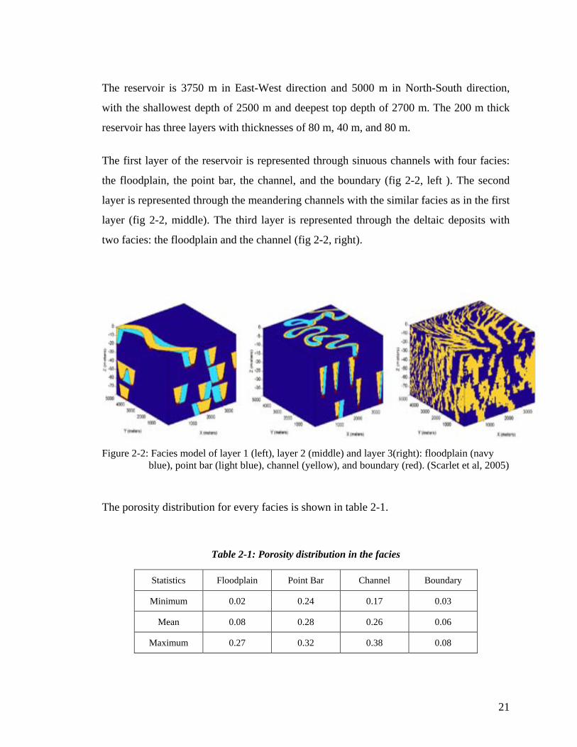
In the equations above, seis(i,j,k,t) and swat(i,j,k,t) represent the seismic amplitude and
water saturation at grid (i,j,k) and time t.
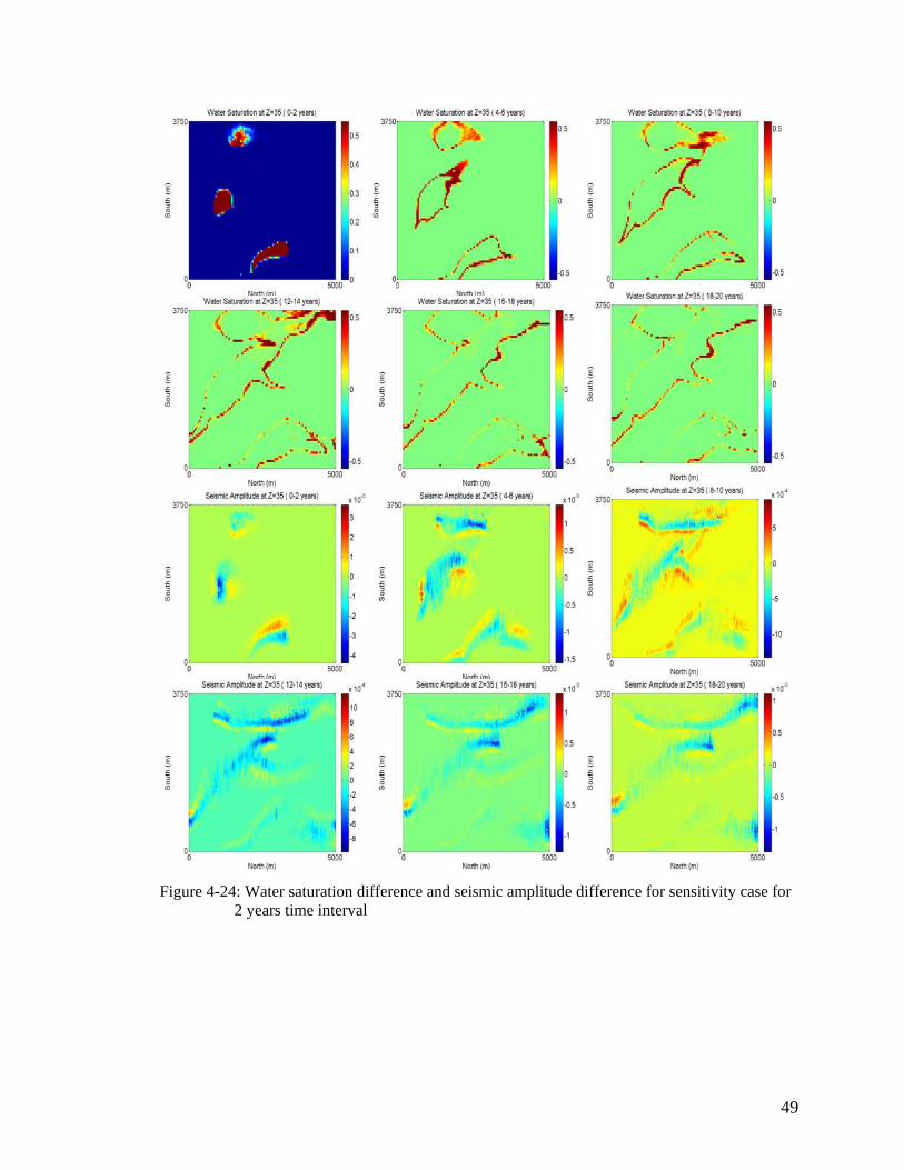
The water saturation change and seismic amplitude change for the base case is shown in
figure 4-1 through 4-3 and for the sensitivity case in figure 4-4 through 4-6. I chose to
show layers 35 in all the plots, because the most of the water went into this layer, thus its
representative of saturation change.
The water saturation change over two years time interval and seismic amplitude change
over the same time interval for layer 35 is shown in figure 4-1. It is apparent that the
water saturation change curve is thinner for 2 years comparing to 4 years, which is
thinner comparing to 10 years as time increases. It happened because the water injection
volume did not change, but the area increased resulting in the thin curve on the boundary
of the water front.
The same concept was observed for the sensitivity case.
46
Figure 4-21: Water saturation difference and seismic amplitude difference base case for 2 years
time interval
47
Figure 4-22: Water saturation difference and seismic amplitude difference base case for 4 years
time interval
48
Figure 4-23: Water saturation difference and seismic amplitude difference for base case for 10
years time interval
49
Figure 4-24: Water saturation difference and seismic amplitude difference for sensitivity case for
2 years time interval
50
Figure 4-25: Water saturation difference and seismic amplitude difference for sensitivity case
with 4 years time interval
51
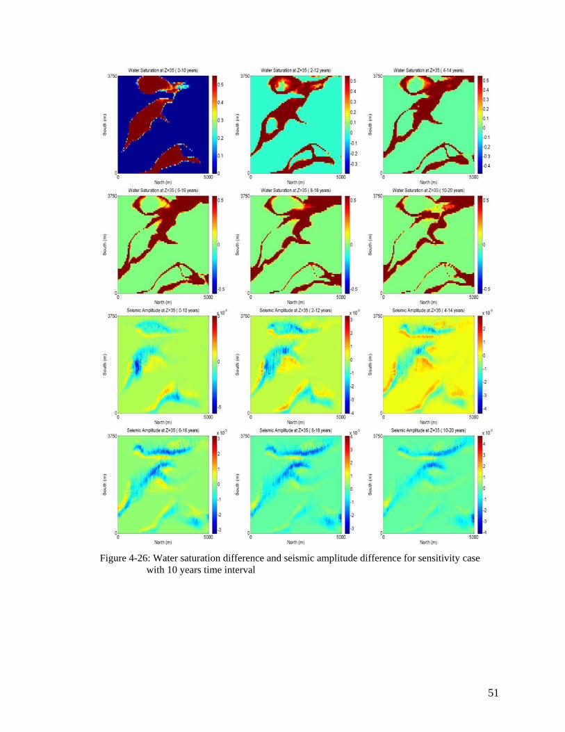
Figure 4-26: Water saturation difference and seismic amplitude difference for sensitivity case
with 10 years time interval
52
4.2. Impact of the Template Window Size on the Correlation
The correlation between the saturation change and seismic amplitude change depends on
the template size, which were studied in this section. The methodology is described
below.
First I evaluated the point-to-point correlation for the base and sensitivity cases for 0-2
years time interval. The correlation was 0.05 and 0.1 for the base and sensitivity case
respectively. The reason for such a poor correlation could be the different support level
between two data sets.
The next step was to consider patterns, which were created by using a 3D template (fig 4-
7). The template size varied in horizontal direction from 3 to 11 grids and in vertical
direction from 1 to 7 grids. The resulting data was used as input parameter into the
principal component analysis (PCA). The PCA is used to reduce the dimensionality and
the first principal components usually are the most representative realizations as they
contain most of the variations. After getting the first and second principal components for
the water saturation change and seismic amplitude change they were standardized. These
data were used to find the correlation.
The results are shown in table 4-1 and 4-2. According to the results horizontal increase of
the template size slightly changes the correlation with increment varying between 0.01
and 0.05. The vertical increase from 1 gird to 3 grids or from 5 grids to 7 girds is not
observed. However when I increased vertical size of the template from 3 to 5 grids, the
correlation increased from 0.05 to 0.71 for the base case and from 0.1 to 0.45 for the
sensitivity case. This template size is approximately equal to Fresnel zone over which we
smoothed out the seismic amplitude. Therefore it is recommended to choose template
size equivalent to Fresnel zone.
53
Table 4-3: Base Case: Correlation between seismic amplitude difference and water saturation difference for 0-2 year time itnerval
Table 4-2: Sensitivity Case: Correlation between seismic amplitude difference and water saturation difference for 0-2 year time itnerval
54
Figure 4-27: a) Horizontal template, b) 3D template for seismic data, c) 3D template for water saturation (Source: Wu, 2003).
55
4.3. Correlation Evolution over Time
The template size of 7x7 was used for this study. The figures illustrate layer 35 as in the previous section.
4.3.1. Base Case
According to the figure 4-8 the correlation coefficient between the second PC of the
seismic data change and the first PC of the water saturation change gives the highest
value of 0.75 for time interval 0-2 and has a declining trend further until it reaches 10-12
time interval, after which it goes up. Whereas the first PC of water saturation change and
the first PC of seismic amplitude change performs slightly better than point-to-point
correlation over the entire 20 years.
Figure 4-9 shows the original water saturation difference and seismic amplitude
difference, first and second PC of water saturation difference and seismic amplitude
difference for time interval 0-2 and 2-4. This when the highest value for the correlation
was obtained. Figure 4-10 shows the same parameters as in figure 4-9, but for time
interval 10-12 and 12-14 years. This is when the worst correlation was obtained.
Figure 4-28: Correlation coefficient for the base case 2 years interval
56
Figure 4-29: Original, first and second PC of saturation change and seismic data change for the base case for time interval 0-2 and 2-4 years
57
Figure 4-30: Original, first and second PC of saturation change and seismic data change for the
base case for time interval 10-12 and 12-14 years
58
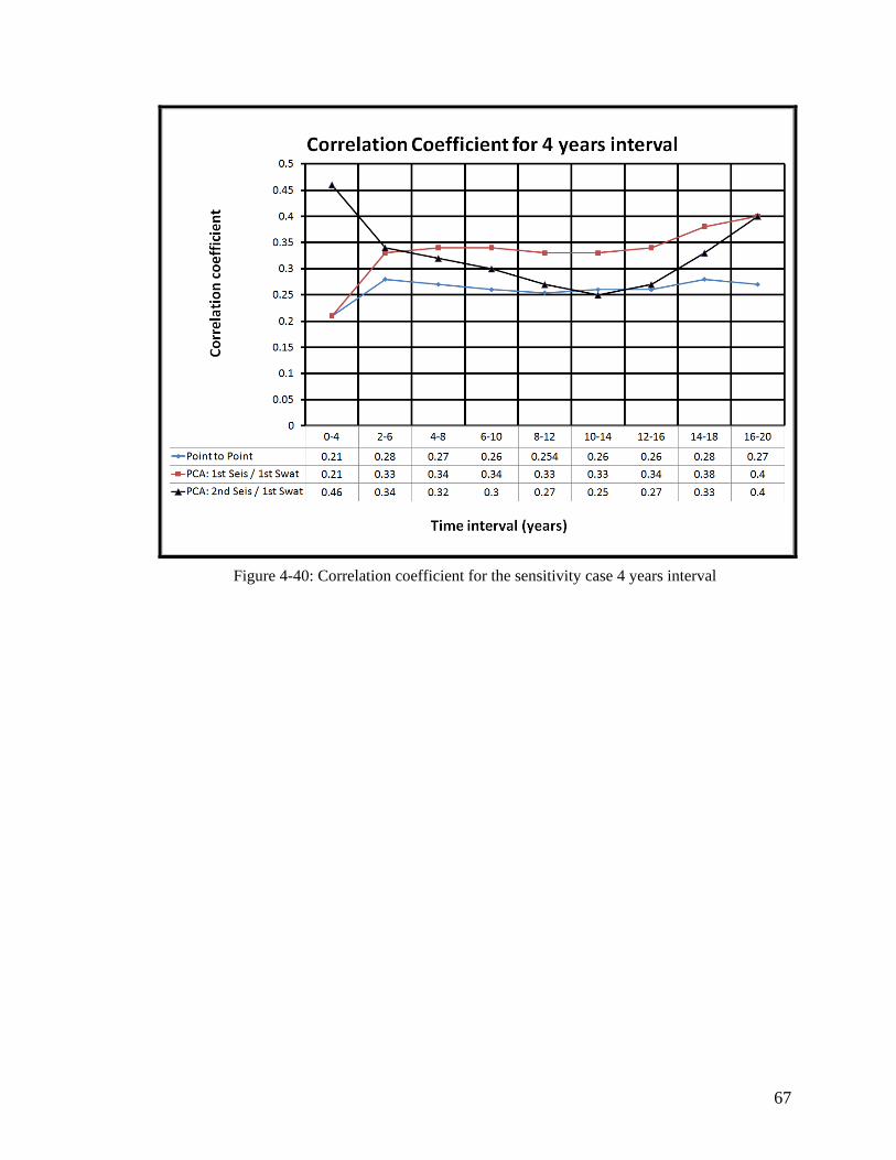
The correlations for the 4 years time interval has the same trend as for 2 years time
difference.
Actually the results repeated findings of Wu’s work. He got the pattern correlation
around 0.7 for time interval 0-2 and 0-4 years.
The apparent reason for the correlation coefficient to decline could be observed in figure
4-9 and 4-10. In figure 4-9 the water saturation change is given as a bulk of water at the
injector location, thus we have seismic amplitude at the same place. In figure 4-10 the
water saturation change is given as a thin curve at the front of the moving water. That
thin curve covers a big area resulting in the spread of the seismic amplitude over that big
area and smoothed by Fresnel zone. It is obvious that in this case the correlation would
be low.
Figure 4-31: Correlation coefficient for the base case 4 years interval
59
Figure 4-32: Original, first and second PC of saturation change and seismic data change for the
base case for time interval 0-4 and 2-6 years
60
Figure 4-33: Original, first and second PC of saturation change and seismic data change for the
base case for time interval 8-12 and 12-16 years
61
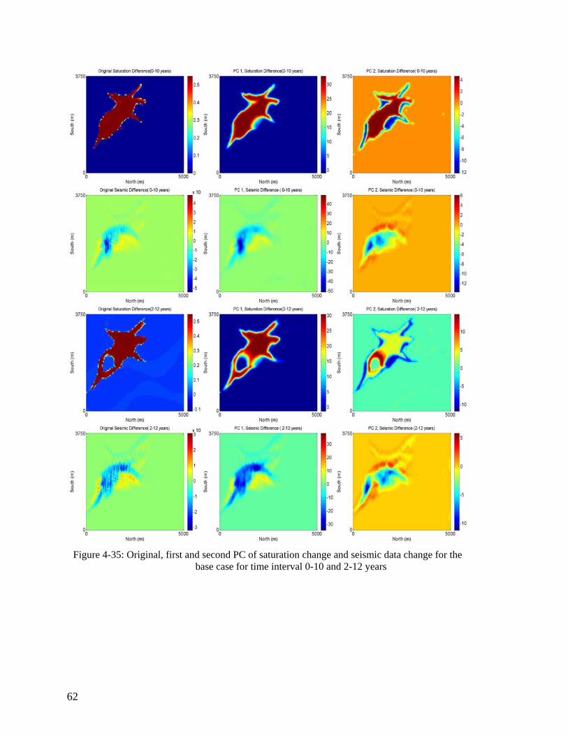
Correlation for 10 years worsened from 0.75 to 0.65, but still follows the same trend as
for 2 and 4 years time interval.
Figure 4-34: Correlation coefficient for the base case 10 years interval
62
Figure 4-35: Original, first and second PC of saturation change and seismic data change for the
base case for time interval 0-10 and 2-12 years
63
Figure 4-36: Original, first and second PC of saturation change and seismic data change for the
base case for time interval 6-16 and 10-20 years
64
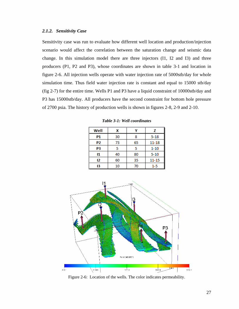
4.1.2. Sensitivity Case
In this case we had three wells injecting water at different location, but with the same
water injection rate. The correlation coefficient worsened form 0.75 to 0.47. This is
happened probably because there were many spots of water saturation change instead of
one. However the same trend is preserved as for the base case.
Also, it is noticeable that the second PC of the seismic data change can work only first 4
years, after that the first PC of the seismic data change shows better correlation.
We observe the same trend for 2, 4 and 10 years.
Figure 4-37 : Correlation coefficient for the sensitivity case 2 years interval
65
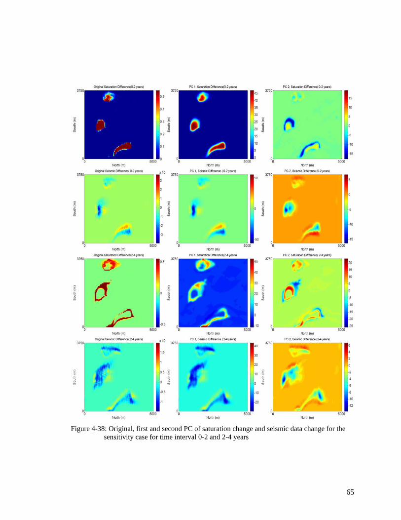
Figure 4-38: Original, first and second PC of saturation change and seismic data change for the
sensitivity case for time interval 0-2 and 2-4 years
66
Figure 4-39: Original, first and second PC of saturation change and seismic data change for the
sensitivity case for time interval 10-12 and 12-14 years
68
Figure 4-41: Original, first and second PC of saturation change and seismic data change for the
sensitivity case for time interval 0-4 and 2-6 years
69
Figure 4-42: Original, first and second PC of saturation change and seismic data change for the
sensitivity case for time interval 8:12 and 12-16 years
71
Figure 4-44: Original, first and second PC of saturation change and seismic data change for the
sensitivity case for time interval 0-10 and 2-12 years
72
Figure 4-45: Original, first and second PC of saturation change and seismic data change for the
sensitivity case for time interval 6-16 and 10-20 years
73
Chapter 5
5. Conclusions and Future Work
5.1. Summary and Conclusions
There was a research work performed to establish the pattern correlation between a
saturation change and seismic data change. According to the results of that study there
was a good pattern correlation (around 0.7) comparing to the poor point-to-point
correlation (around 0.3) between the saturation change and seismic data change. The
reason for this was a different support level between the seismic data and saturation data.
That work was performed for one injector and one producer operating under the constant
conditions in the second layer of Stanford V reservoir model for two years.
We conducted the further study of the pattern correlation. Particularly we studied what
kind of impact a different template size, well location and production/injection scenario
would have on the correlation. Also the correlation evolution was observed for 20 years
of production/injection period for time intervals of 2, 4 and 10 years. To conduct the
studies mentioned above the first layer of Stanford VI reservoir model was used, which
was more complex than Stanford V.
The data preparation part of the workflow included several procedures such as the fluid
flow simulation to obtain the saturation at different times and the forward seismic
simulation to obtain the time-lapse seismic data. There were two flow simulation
scenarios run: base case with two wells and sensitivity case with six wells. After the data
set was ready the seismic difference and saturation difference cubes were generated for 2,
4 and 10 years time intervals. Further we used the template (moving window) to generate
several realizations of the data set. These realizations were input for the principal
component analysis, which provided the principal components. The first and second
principal components accounted for the most variations in the data set. This modified
74
data set was used to evaluate the correlation between the saturation change and seismic
data change.
The study of the template size affect on the correlation showed that the increase of the
template size in the horizontal direction improves the correlation slightly, but the increase
in the vertical direction has a significant impact. In our case for example the increment of
the correlation varied between 0.01 and 0.05 when the template size was increased
horizontally. The increment of the correlation jumped from 0.4 to 0.6 when in vertical
direction the grid numbers increased from 3 to 5. But should be mentioned that there
were no effect when the grid size increased from 1 to 5 and from 5 to 7. I guess this one
is associated with Fresnel zone and filtering we used for the seismic data. So the best
would be to have the template size that accounts for the Fresnel zone.
The evolution of the correlation over the time showed two behaviors. First that the
correlation for the first principal component of seismic cube and the first component of
the saturation is better than the point-to-point correlation, but not much. Second is that
the correlation between the second principal component of the seismic amplitude
difference cube and the first component of the water saturation difference cube has a
good correlation coefficient of about 0.76 for the base case and 0.45 for the sensitivity
case for the first time interval of 2 and 4 years. This value is not constant, actually it
declines and reaches point-to-point correlation, after which it goes up. The reason for that
could be that in the beginning the water moves as a bulk of water and it correlates with
the seismic data change. But when for example time interval of 12-14 year is taken, then
the change in water saturation is usually represented by a thin curve on the front of the
water move. Such a small change gives the seismic response that is smoothed out over
the large area, thus reduces the correlation.
The above two studies was carried out for the base case with the one injection well and
one production well. In the sensitivity case three injectors and 3 producers were used.
The correlation was poorer than the base case.
75
5.2. Future Work
In this study I explored the correlation between the water saturation change and seismic
amplitude change under the different conditions. There are still some other methods and
techniques to improve understanding of the correlation between two data type of the data
sets:
• Pressure change also has an impact on the seismic data set, thus on the
correlation. Moreover there is a study that shows that the effect of the pressure
change should not be neglected as it has significant impact (Suman, 2009). Thus it
would be of interest to incorporate the pressure change when constructing the
seismic amplitudes and study how it affects the correlation.
• The synthetic models are very important in testing concepts, but the application of
this method to the real reservoir data set is of main importance. The next step
could be to try this method on a real reservoir data set and see what correlation
could be obtained under the real conditions.
• Kernel Principal Component Analysis has proven to be effective tool in working
with patterns than Principal Component Analysis. Also it is good to detect
curvatures.
77
Nomenclature
amp = Seismic amplitude imp = Seismic impedance ρ = Bulk density ρfl = Fluid density φ = Porosity ρfl1 = Fluid density for fluid 1 ρfl2 = Fluid density for fluid 2 Vp = Compressional velocity Vs = Shear velocity K2 = Bulk modulus for fluid 2 G2 = Shear modulus for fluid 2 Kmin = Bulk modulus of the mineral
Kfl = Bulk modulus of the fluid Kfl1 = Bulk modulus of the fluid 1
Kfl2 = Bulk modulus of the fluid 2
ttop = Two way travel time from the surface to the top of the reservoir ∆t = Two way travel time from the top to the bottom of the grid t = Two way travel time from the surface to the bottom of the grid seis(i,j,k,t) = Seismic amplitude at grid location (i,j,k) at time (t) swat(i,j,k,t) = Water saturation at grid location (i,j,k) at time (t) δseis(i,j,k,t) = Seismic Amplitude difference δswat(i,j,k,t) = Water Saturation difference
78
References
Aziz, K., Durlofsky, L., and Tchelepi, H., 2005, "Notes on Reservoir Simulation", Stanford University, Stanford, CA.
Beucher, H., Fournier, F., Doligez, B., and Rozanski, J., 1999, "Using 3D seismic-
derived information in lithofacies simulations. A case study", Paper SPE 56736, SPE Annual Technical Conference and Exhbition, Houston, TX.
Caers, J., 2005, “Petroleum Geostatistics”, Society of Petroleum Engineers. Castro, S., Caers, J. and Mukerji, T., 2005, “The Stanford VI Reservoir”, Stanford
Center for Reservoir Forecasting, Annual Report. Castro, S., 2007, “A Probabilistic Approach to the Joint Integration of 3D/4D
Seismic, Production Data and Geological Information for Building Reservoir Models”, PhD thesis, Stanford University, Stanford, CA.
Chen, G., Wrobel, Kelly., Tiwari, A., Zhang, J. and Payne, M., 2008, “4D Seismic in
Carbontes: From Rock Physics to Field Examples”, Paper IPTC 12065, International Petroleum Technology Conference, Kuala Lumpur, Malaysia.
Foster, D.G., 2007, “The BP 4-D Story: Experience Over the Last 10 Years and
Current Trends”, International Petroleum Technology Conference, Dubai, U.A.E. Gassmann, F., 1951, Über die Elastizität poroser Medien, Vierteljahrsschrift der
Naturforschenden Gesellschaft in Zürich, 96, 1-23. Goovaerts, P., 1997, “Geostatistics for Natural Resources Evaluation”, Oxford
University Press, New York. Jolliffe, I., 1986, “Principal Component Analysis”, Springer-Verlag, New York. Kelamis, P.G., Uden, R.C. and Dunderdale, I., 1997, “4D Seismic Aspects of
Reservoi Managment”, Paper OTC 8293, Offshore Technology Conference, Houston, TX.
79
Marschall, R. and Sherlock, D., 2002, “Some Aspects of 4-D Seismics for Reservoir
Monitoring”, Paper SPE 75150, SPE Improved Oil Recovery Symposium, Tulsa, OK.
Mukerji, T., Jorstad, A., Avseth, P., Mavko, G. and Granli, J., 2001, “Mapping
Lithofacies and Pore-Fluid Probabilities in a North Sea reservoir: Seismic Inversion and Statistical Rock Physics”, Geophysics 66(4), 988-1001.
Mukerji, T., Mavko, G., Mujicat, D. and Lucet, N., 1995, “Scale-Dependent Seismic
Velocity in Heterogeneou Media”, Geophysics 60 (4), 1222-1233. Mukerji, T., Mavko, G., and Rio, N., 1997, “Scales of Reservoir Heterogeneities and
Impact of Seismic Resolution of Geostatistical integration”, Mathematical Geology 29, 933-949.
Sheriff, R. and Geldart, L., 1995, “Exploration Seismology”, Second Edition,
Cambridge University Press. Scheeven, J.R. and Payrazyan, K., 1999, “Principal Component Analysis Applied to
3D Seismic Data for Reservoir Property Estimation”, Paper SPE 56734, SPE Annual Technical Confrence and Exhibition, Houston, TX.
Suman A., 2009, "Uncertainties in Rock Pore Compressibility and Effects on Seismic
History Matching", MS Thesis, Stanford University, Stanford, CA. Wu, J., 2007, “4D Seismic and Multiple-Point Pattern Data Integration Using
Geostatistics”, PhD thesis, Stanford University, Stanford, CA.