STUDY OF PORE SIZE EFFECT IN CHROMATOGRAPHY BYVIBRATIONAL SPECTROSCOPY AND COLLOIDAL ARRAYS
Item Type text; Electronic Dissertation
Authors Huang, Yuan
Publisher The University of Arizona.
Rights Copyright © is held by the author. Digital access to this materialis made possible by the University Libraries, University of Arizona.Further transmission, reproduction or presentation (such aspublic display or performance) of protected items is prohibitedexcept with permission of the author.
Download date 18/06/2018 06:55:41
Link to Item http://hdl.handle.net/10150/196108
STUDY OF PORE SIZE EFFECT IN CHROMATOGRAPHY BY VIBRATIONAL
SPECTROSCOPY AND COLLOIDAL ARRAYS
by
Yuan Huang
A Dissertation Submitted to the Faculty of the
DEPARTMENT OF CHEMISTRY
In partial Fulfillment of the Requirements
For the Degree of
DOCTOR OF PHILOSOPHY
In the Graduate College
THE UNIVERSITY OF ARIZONA
2008
2
THE UNIVERSITY OF ARIZONA
GRADUATE COLLEGE
As members of the Dissertation Committee, we certify that we have read the dissertation
prepared by Yuan Huang
entitled “Study of Pore Size Effect in Chromatography by Vibrational Spectroscopy and
Colloidal Arrays ”
and recommend that it be accepted as fulfilling the dissertation requirement for the
Degree of Doctor of Philosophy
_______________________________________________________________________ Date: 11/21/08
Dr. Jeanne E. Pemberton
_______________________________________________________________________ Date: 11/21/08
Dr. Neal R. Armstrong
_______________________________________________________________________ Date: 11/21/08
Dr. S. Scott Saavedra
_______________________________________________________________________ Date: 11/21/08
Dr. Eugene A. Mash, Jr.
Final approval and acceptance of this dissertation is contingent upon the candidate’s
submission of the final copies of the dissertation to the Graduate College.
I hereby certify that I have read this dissertation prepared under my direction and
recommend that it be accepted as fulfilling the dissertation requirement.
________________________________________________ Date: 11/21/08
Dissertation Director: Jeanne E. Pemberton
STATEMENT BY AUTHOR
This dissertation has been submitted in partial fulfillment of requirements for an
advanced degree at The University of Arizona and is deposited in the University Library
to be made available to borrowers under rules of the library.
Brief quotations from this dissertation are allowable without special permission,
provided that accurate acknowledgement of source is made. Request for permission for
extended quotation from or reproduction of this manuscript in whole or in part may be
granted by the head of the major department or the Dean of the Graduate College when in
his or her judgment the proposed use of the material is in the interests of scholarship. In
all other instances, however, permission must be obtained from the author.
SIGNED: Yuan Huang
4
TABLE OF CONTENTS
LIST OF FIGURES .............................................................................................................9
LIST OF TABLES .............................................................................................................17
ABSTRACT .......................................................................................................................18
CHAPTER 1: INTRODUCTION TO SEPARATION PROCESSES IN
CHROMATOGRAPHY ..........................................................................20
Thermodynamic processes in column chromatography ................................................20
Ion-stationary phase interactions in ion chromatography:
Stationary phase selectivity ............................................................................................23
Retention models in reversed phase liquid chromatography .........................................27
Solvophobic model .....................................................................................................28
Partition model ..........................................................................................................29
Comparison of solvophobic
model and partition model .........................................................................................32
Mobile phase composition .............................................................................................34
Diffusion of molecules in chromatography columns:
Dynamics in separation systems ..................................................................................37
Effects of molecular diffusion on separation performance ............................................40
Goals of this research .....................................................................................................43
CHAPTER 2: EXPERIMENTAL...................................................................................45
Materials ........................................................................................................................45
Instrumentation ..............................................................................................................46
Raman spectroscopy ..................................................................................................46
Fourier transform infrared spectroscopy (FTIR) ......................................................47
Scanning electron microscopy (SEM) ........................................................................50
Methodology ..................................................................................................................50
Raman spectral analysis ............................................................................................50
5
TABLE OF CONTENTS - continued
Silica particle size and size distribution characterization .........................................51
CHAPTER 3: CHARACTERIZATION OF STRONG ANION
EXCHANGE STATIONARY PHASE BY
RAMAN SPECTROSCOPY ...................................................................52
Introduction ....................................................................................................................52
Instrumentation and experimental procedures ...............................................................59
Results and discussion ...................................................................................................59
Raman spectra of Isolute SAX stationary phases ......................................................59
Stationary phase selection .........................................................................................69
Characterization of stationary phase by Raman spectroscopy..................................71
Conclusions ....................................................................................................................87
CHAPTER 4: OPTIMIZATION OF REACTION CONDITIONS USING
MODIFIED LAMER MODEL FOR THE FABRICATION OF
UNIFORM AND SPHERICAL SUB-100
NM SILICA PARTICLES ........................................................................88
Introduction ....................................................................................................................88
Experiments ...................................................................................................................92
Preparation of silica nanoparticles ...........................................................................92
Results and discussion ...................................................................................................93
Chemical reactions in Stöber system .........................................................................93
Models describing particle formation and growth
by the Stöber method ..................................................................................................94
Classic LaMer model for particle formation and
Growth: A general introduction.................................................................................97
The Modified LaMer model .....................................................................................101
Optimization strategies for sub-100 nm particle synthesis using the modified
LaMer plot ...............................................................................................................106
Correlation between modified LaMer plot and particle properties.........................107
Changing modified LaMer plot by changing reaction conditions ...........................111
Duration of nucleation process ............................................................................111
Final particle number ..........................................................................................112
Growth Factor .....................................................................................................113
Optimization of reaction conditions for sub-100 nm particle synthesis ..................114
6
TABLE OF CONTENTS - continued
Initial reaction conditions ....................................................................................114
Stöber method by very high hydrolysis rate and the corresponding
Modified LaMer plot ............................................................................................115
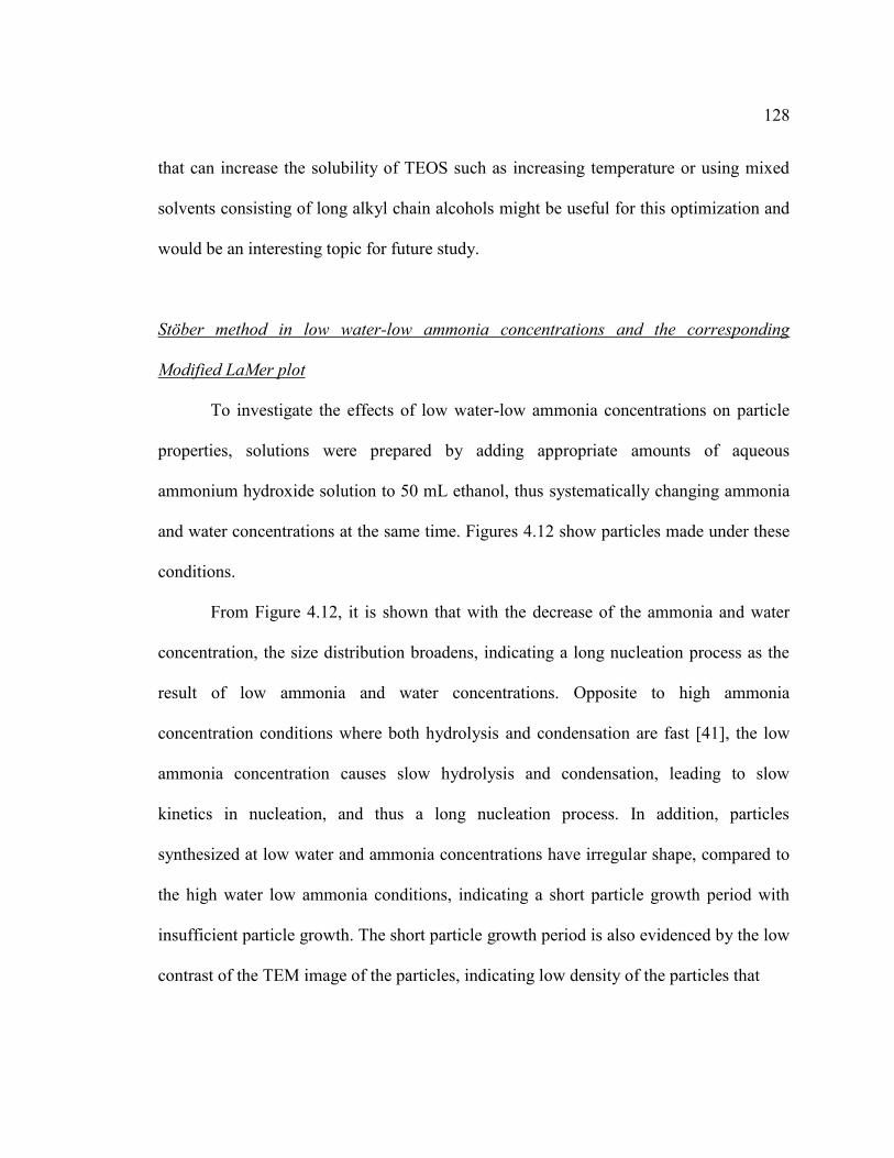
Stöber method in low water-low ammonia concentrations and the
corresponding modified LaMer plot ....................................................................128
Optimizing reaction conditions of low ammonia low water systems for
synthesis of uniform and spherical sub-100 nm silica particles ..........................136
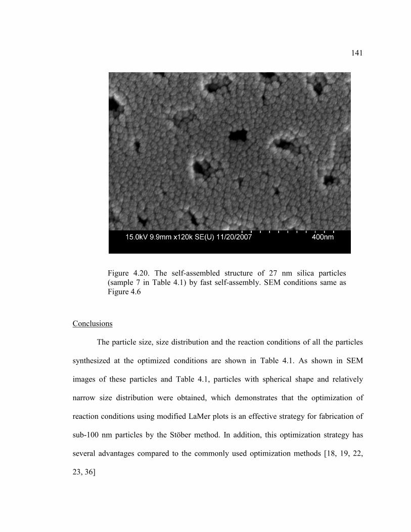
Conclusions ..................................................................................................................141
CHAPTER 5: FABRICATION OF COLLOIDAL ARRAY BY THE
SELF ASSEMBLY OF SUB-100 NM
SILICA PARTICLES .............................................................................144
Introduction ..................................................................................................................144
Experimental ................................................................................................................147
Fabrication and purification of silica particles .......................................................147
Self-assembly of the nanoparticles by vertical evaporation ....................................148
Results and discussion .................................................................................................149
Self-assembly mechanism of particles to three dimensional structures...................149
Effect of particle properties on the packing quality.................................................152
Three dimensional colloidal array made of sub-100 nm
silica particles made by The Stöber method ............................................................154
Temperature effects on the packing quality .............................................................156
Effects of particle concentration in solutions on the packing quality ......................161
Experiments of self-assembled monolayer structure ...............................................162
Fast self-assembly by horizontal evaporation .........................................................164
Conclusions ..................................................................................................................178
CHAPTER 6: IN SITU ATR-FTIR KINETIC STUDIES OF MOLECULAR
DIFFUSION IN NANOPORES OF SILICA COLLOIDAL
THIN FILMS .........................................................................................180
Introduction ..................................................................................................................180
Experimental ................................................................................................................184
Reagents and silica film preparation .......................................................................184
Attenuated Total Reflection-Fourier Transform Infrared Spectroscopy .................185
7
TABLE OF CONTENTS - continued
Results and discussions ................................................................................................186
Pores in the colloidal arrays....................................................................................186
Diffusion models for diffusion coefficient information extraction ...........................187
Simplifying the diffusion models ..............................................................................193
Diffusion spectra of molecules in pore ....................................................................197
Measuring diffusion coefficients in colloidal arrays made of 50nm particles.........199
Diffusion of molecules in nanopores........................................................................201
Mechanism of diffusion in nanopores ......................................................................204
Conclusions ..................................................................................................................213
CHAPTER 7: ATR-FTIR STUDIES OF WATER-ACETONITRILE
DISTRIBUTION IN NANOPORES OF SILICA COLLOIDAL
ARRAY THIN FILMS. .........................................................................215
Introduction ..................................................................................................................215
Experimental ................................................................................................................218
Reagents and Silica Silm Preparation .....................................................................218
Attenuated Total Reflection-Fourier Transform Infrared Spectroscopy .................219
Results and Discussions ...............................................................................................219
A general model (single phase model) for calculating mole
fraction of acetonitrile in pores ...............................................................................219
Derivation of the two-phase model for calculating absorbance caused by
adsorption in pores ..................................................................................................232
Applying the two-phase model for calculating film thickness .................................235
Applying the two-phase model for calculating acetonitrile mole fraction ..............237
Chromatographic implications ................................................................................239
Conclusions ..................................................................................................................244
CHAPTER 8. CONCLUSIONS AND FUTURE DIRECTIONS ...................................246
Characterization of interactions in ion exchange chromatography ..............................246
Sub-100 nm silica particle synthesis and self-assembly ..............................................247
Measurement of diffusion coefficients of molecules in nanopores .............................248
Measurement of organic modifier distribution in nanopores .......................................249
8
TABLE OF CONTENTS - continued
Future directions ..........................................................................................................250
Amount of molecules in nanopores ..........................................................................250
Pore size effect on molecular diffusion in nanopores ..............................................253
Temperature effect on molecular diffusion in nanopores ........................................254
Effect of pore wall modifications on molecular diffusion in nanopores ..................255
Effects of adsorption on diffusion coefficient in pores.............................................256
Distribution of organic modifiers in hydrophobic pores .........................................258
Effects of pressures on distribution of organic modifiers
in hydrophobic pores ..............................................................................................259
APPENDIX A: MEASUREMENT OF THE SURFACE
AREA OF PARTICLE ARRAYS BY QUARTZ
CRYSTAL MICROBALANCE (QCM) ............................................261
Experimental ................................................................................................................265
Results and discussion .................................................................................................265
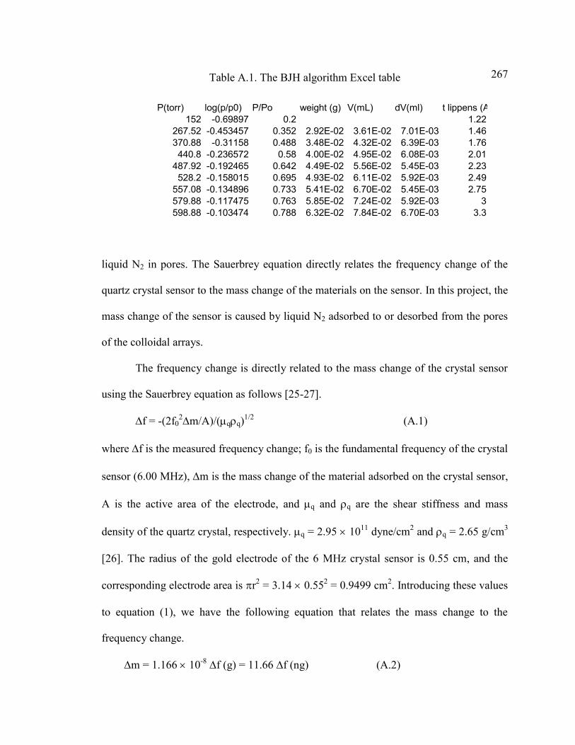
Implementation of BJH algorithm for PSD calculations .........................................265
Feasibility experiments ............................................................................................266
Measurement of surface area of colloidal array by thickness monitor ...................270
Conclusions ..................................................................................................................281
APPENDIX B: RAMAN SPECTRA OF SAX STRONG ANION EXCHANGE
STATIONARY PHASE IN STRONG ACIDS ................................282
REFERENCES ................................................................................................................289
9
LIST OF FIGURES
FIGURE 2.1 Block diagram of Raman spectrometer system ........................................48
FIGURE 2.2 Schematic diagram of ATR-FTIR
experiment set-up .....................................................................................49
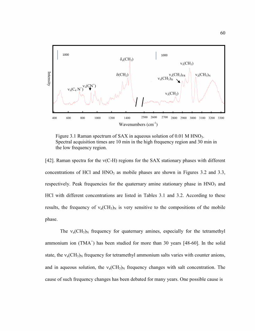
FIGURE 3.1 Raman spectrum of SAX in aqueous solution of 0.01 M
HNO3. Spectral acquisition times are 10 min in the high frequency
region and 30 min in the low frequency region. ......................................60
FIGURE 3.2 Raman spectra of SAX-HCl in ν(C-H) region for aqueous solutions of
(a) 6, (b) 2, and (c) 0.01 M HCl ...............................................................61
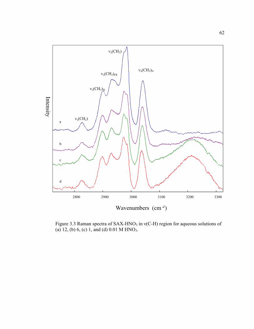
FIGURE 3.3 Raman spectra of SAX-HNO3 in ν(C-H) region for aqueous solutions of
(a) 12, (b) 6, (c) 1, and (d) 0.01 M HNO3 ................................................62
FIGURE 3.4 Frequency of the a(CH3)N of SAX as a function of electrolyte
concentration in aqueous mobile phase ...................................................72
FIGURE 3.5 a(CH3)N frequencies for mixed HCl-LiCl ...............................................73
FIGURE 3.6 Raman Spectra of SAX from 400 to 1600 cm-1
in
(A) 6M HCl and (B) 6 M HNO3 within (a) 1 hour
and (b) after 24 days. Acquisition time is 30 min ....................................81
FIGURE 3.7 Raman Spectra of SAX in (C-H) region in
(A) 6M HCl and (B) 6 M HNO3 within (a) 1 hour
and (b) after 24 days. Acquisition time is 10 min ....................................83
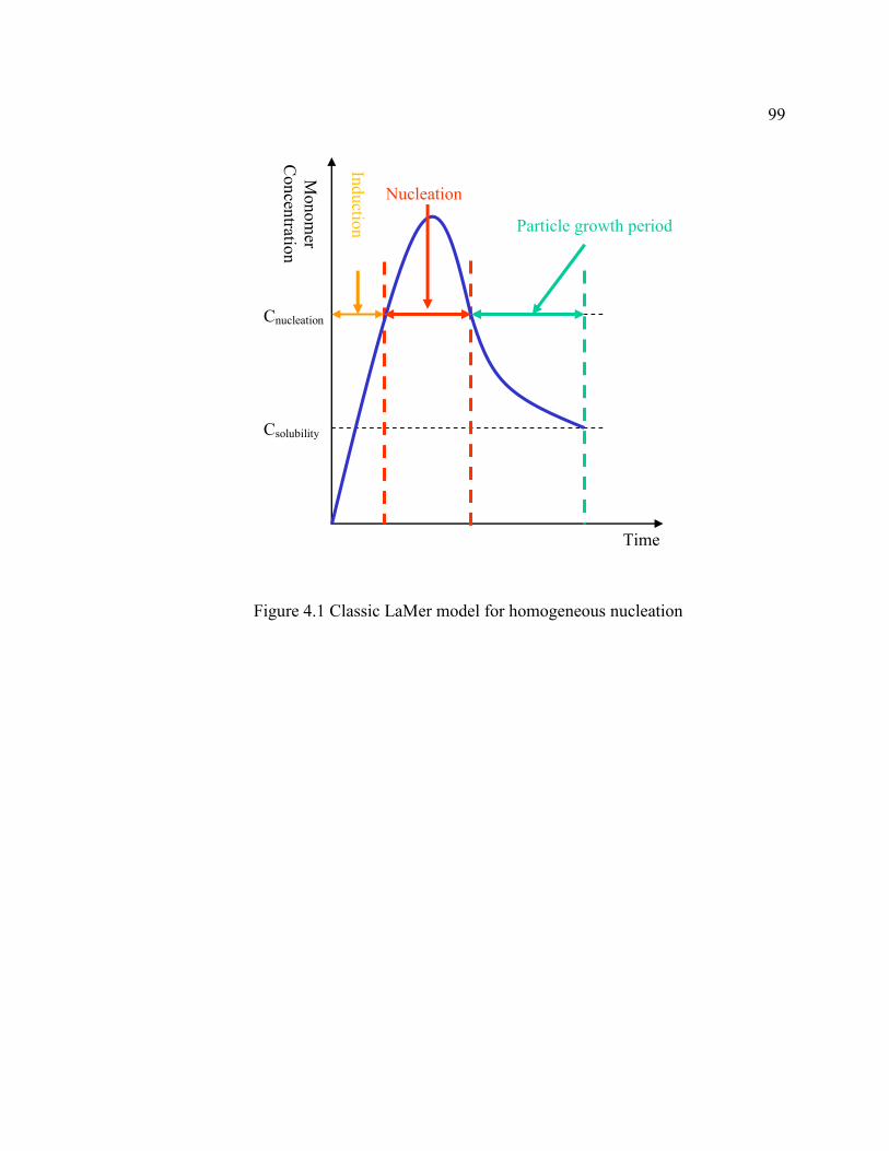
FIGURE 4.1 Classic LaMer model for homogeneous nucleation .................................99
FIGURE 4.2 Interpretation of the concept of the “nucleation burst”
by the classic LaMer model ..................................................................102
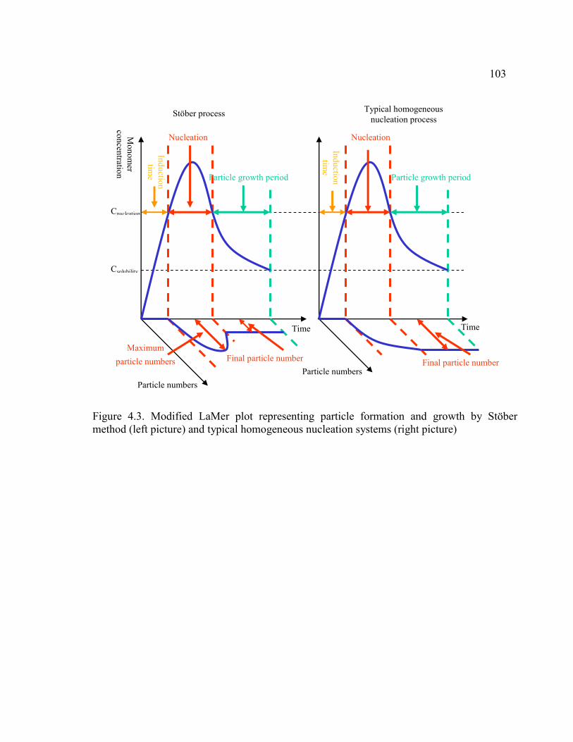
FIGURE 4.3 Modified LaMer plot representing particle formation and growth by
Stöber method (left picture) and typical homogeneous
nucleation systems (right picture) ..........................................................103
FIGURE 4.4 Proposed optimization strategy for
sub-100 nm silica particle synthesis ......................................................107
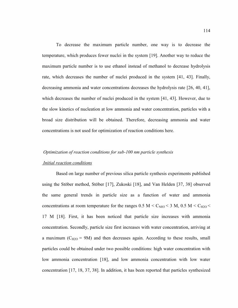
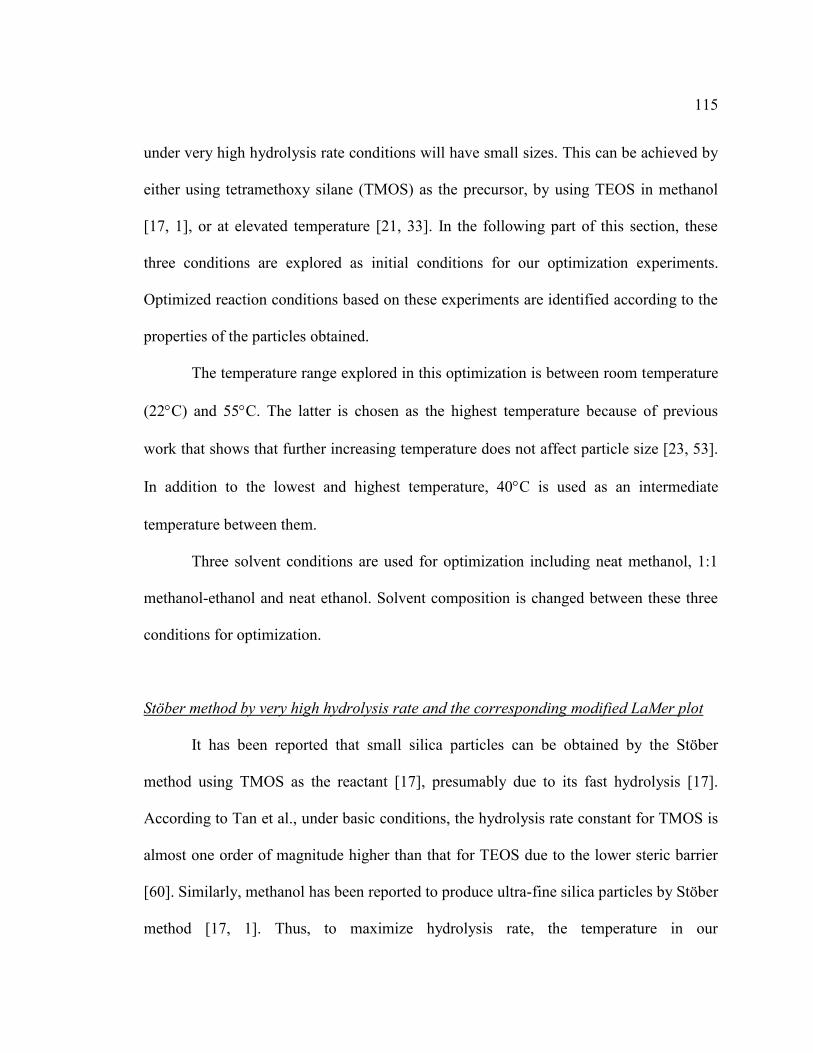
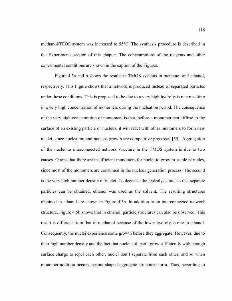
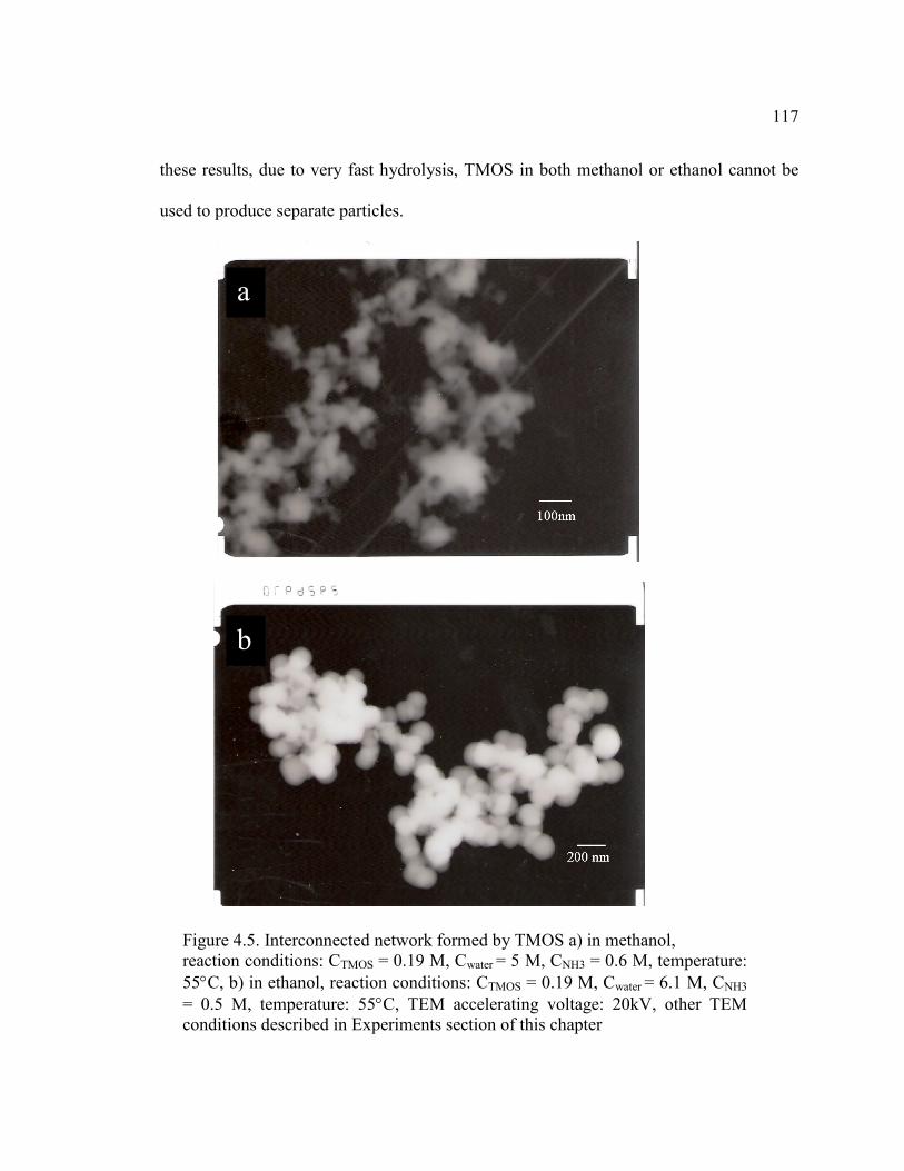
FIGURE 4.5 Interconnected network formed by TMOS a) in methanol,
reaction conditions: CTMOS = 0.19 M, Cwater = 5 M,
10
LIST OF FIGURES – Continued
CNH3 = 0.6 M, temperature: 55C, b) in ethanol, reaction conditions:
CTMOS = 0.19 M, Cwater = 6.1 M, CNH3 = 0.5 M, temperature: 55C,
TEM accelerating voltage: 20kV, other TEM conditions described in
Experiments section of this chapter .......................................................117
FIGURE 4.6 Particles synthesized in 50 mL methanol at 55 C with different
volumes of 2:1 NH4OH:H2O added. a) 6 mL 2:1 NH4OH-H2O;
b) 9 mL 2:1 NH4OH-H2O (particle size, 35 nm, irregular);
c) 12 mL 2:1 NH4OH-H2O (particle size, 70 nm, irregular);
d) 15 mL 2:1 NH4OH-H2O (particle size, 85 nm, irregular) added.
Other synthesis conditions and procedures are described in
Experiments section of this Chapter. SEM operation parameters
for top surface imaging are described in Chapter 2 ...............................119
FIGURE 4.7 Modified Graphic LaMer plot for
TEOS in methanol at elevated temperature ...........................................121
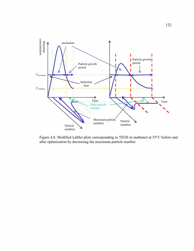
FIGURE 4.8 Modified LaMer plots corresponding to TEOS in methanol at
55C before and after optimization by decreasing
the maximum particle number ...............................................................122
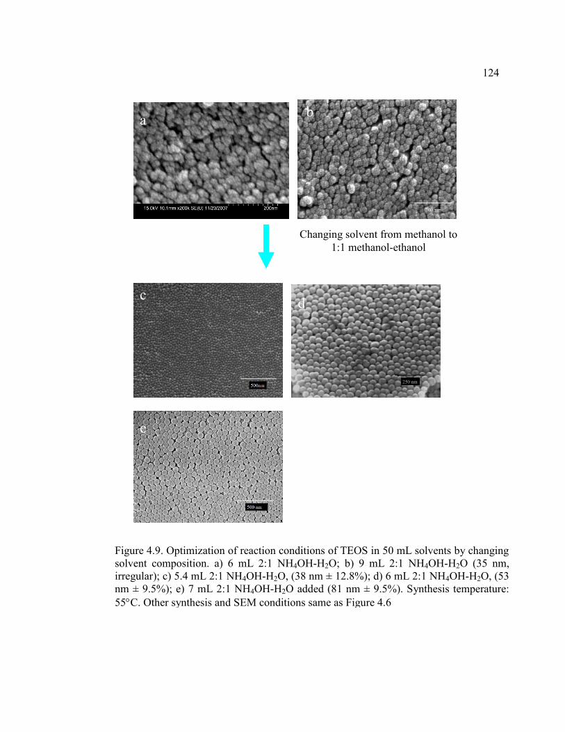
FIGURE 4.9 Optimization of reaction conditions of TEOS in 50 mL solvents
by changing solvent composition. a) 6 mL 2:1 NH4OH-H2O;
b) 9 mL 2:1 NH4OH-H2O (35 nm, irregular);
c) 5.4 mL 2:1 NH4OH-H2O, (38 nm ± 12.8%);
d) 6 mL 2:1 NH4OH-H2O, (53 nm ± 9.5%);
e) 7 mL 2:1 NH4OH-H2O added (81 nm ± 9.5%).
Synthesis temperature: 55C. Other synthesis and SEM
conditions same as Figure 4.6 .................................................................124
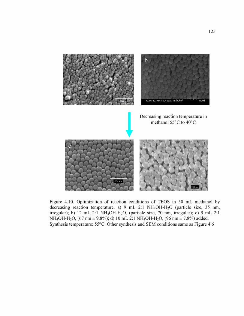
FIGURE 4.10 Optimization of reaction conditions of TEOS in 50 mL
methanol by decreasing reaction temperature.
a) 9 mL 2:1 NH4OH-H2O (particle size, 35 nm, irregular);
b) 12 mL 2:1 NH4OH-H2O, (particle size, 70 nm, irregular);
c) 9 mL 2:1 NH4OH-H2O, (67 nm ± 9.8%);
d) 10 mL 2:1 NH4OH-H2O, (96 nm ± 7.8%) added.
Synthesis temperature: 55C. Other synthesis and
SEM conditions as Figure 4.6 .................................................................125
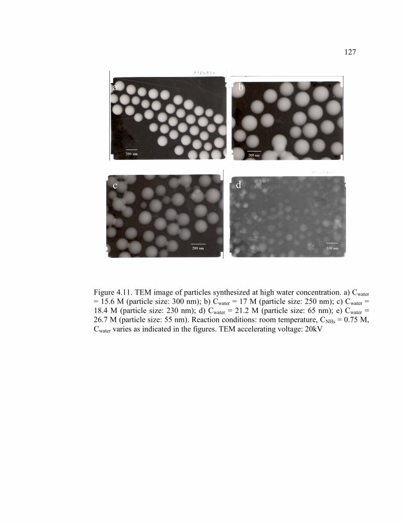
FIGURE 4.11 TEM image of particles synthesized at high water concentration.
a) Cwater = 15.6 M (particle size: 300 nm);
11
LIST OF FIGURES – Continued
b) Cwater = 17 M (particle size: 250 nm);
c) Cwater = 18.4 M (particle size: 230 nm);
d) Cwater = 21.2 M (particle size: 65 nm);
e) Cwater = 26.7 M (particle size: 55 nm).
Reaction conditions: room temperature, CNHs = 0.75 M,
Cwater varies as indicated in the figures.
TEM accelerating voltage: 20 kV ..........................................................127
FIGURE 4.12 TEM image of particles synthesized at low water low ammonia
concentration. a) 4mL NH4OH (particle size: 240nm);
b) 3mL NH4OH (particle size: 105 nm);
c) 2.5 mL NH4OH (particle size: 42 nm);
d) 2 mL NH4OH added (particle size: 40 nm).
Reaction conditions: 50 mL ethanol, at room temperature,
CNHs = 0.75 M. Other synthesis conditions same as Figure 4.6.
TEM condition: 20kV accelerating voltage ...........................................129
FIGURE 4.13 Modified LaMer plot for TEOS in low concentrations of water and
ammonia conditions ...............................................................................132
FIGURE 4.14 Modified LaMer plot for Pontoni et al’s reaction conditions [49] .........134
FIGURE 4.15 TEM image of particles made under reaction conditions
similar to those used by Pontoni et al. [49]
(Reaction conditions: [NH3] = 1.45 M and [H2O] = 4.0 M,
and [TEOS] = 0.085 M, average particle diameter = 280 nm).
Other synthesis conditions same as Figure 4.6.
TEM conditions: accelerating voltage: 20kV. .......................................135
FIGURE 4.16 A proposed mechanism for the low Growth Factor of silica particle
at low ammonia and low water concentration conditions ......................136
FIGURE 4.17 Enhancement of particle growth by complete hydrolysis of ethoxyl on
particle surfaces .....................................................................................138
FIGURE 4.18 Modified LaMer plots corresponding to the optimization of low
water low ammonia reaction conditions ................................................139
FIGURE 4.19 Optimization of low ammonia and low water concentration
conditions by increasing reaction temperature and adding more
water. (a) 3 mL NH4OH (particle size: 105 nm),
(b) 2.5 mL NH4OH (particle size: 42 nm),
12
LIST OF FIGURES – Continued
(c) 2 mL NH4OH(particle size: 40 nm),
(d) 2.8 mL NH4OH + 1.2 mL H2O ( 49 nm ± 9.5%),
(e) 2.1 mL NH4OH + 0.9 mL H2O added (27 nm ± 13.3%).
Other synthesis conditions same as Figure 4.6. SEM conditions
same as figure 4.6 and TEM same as Figure 4.5 ...................................140
FIGURE 4.20 The self-assembled structure of 27 nm silica particles
(sample 7 in Table 4.1) by fast self-assembly. SEM
conditions same as Figure 4.6 ................................................................141
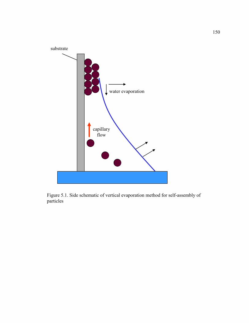
FIGURE 5.1 Side schematic of vertical evaporation method for self-assembly of
particles ..................................................................................................150
FIGURE 5.2 Front schematic of vertical evaporation method for
self-assembly of particles .......................................................................151
FIGURE 5.3 SEM (top view) of self-assembled structures made by different methods.
Sample a) 0.2 wt% ethanol suspension of sample 4 listed in table 1;
sample b) 0.2 wt% ethanol suspension of particles made by The Stöber
method in ethanol at room temperature; sample c).
0.15 wt% ethanol suspension of particles made
by the reverse micelle method ................................................................153
FIGURE 5.4 SEM image (side view) of closely packed three-dimensional structures
made by some of silica particle samples described in Chapter 4
using 0.2 wt% particle suspensions. Sample number
corresponding to the synthesis conditions listed in Table 4.1.
(a) sample 3 (81 nm);
(b) sample 2 (67 nm); (c) sample 4 (53 nm);
(d) sample 6 (38 nm) ..............................................................................155
FIGURE 5.5 SEM images (top view) of close-packed three-dimensional structures
made by silica particle samples using appropriate concentrations
of particle suspensions. a)250 nm, 1.0wt%; b) 120 nm, 0.5wt%;
c) 80 nm, 0.2wt%; d) 53 nm, 0.2wt% particle suspension.....................157
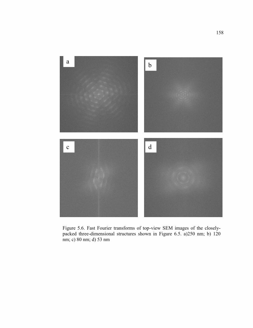
FIGURE 5.6 Fast Fourier transforms of top-view SEM images of
the closely-packed three-dimensional structures shown in
Figure 6.5. a)250 nm; b) 120 nm; c) 80 nm; d) 53 nm ..........................158
FIGURE 5.7 SEM image (top view) of three-dimensional structures
made by 50 nm silica particles using 0.2 wt% particle
13
LIST OF FIGURES – Continued
suspensions at a) 40C; b) 50C ............................................................159
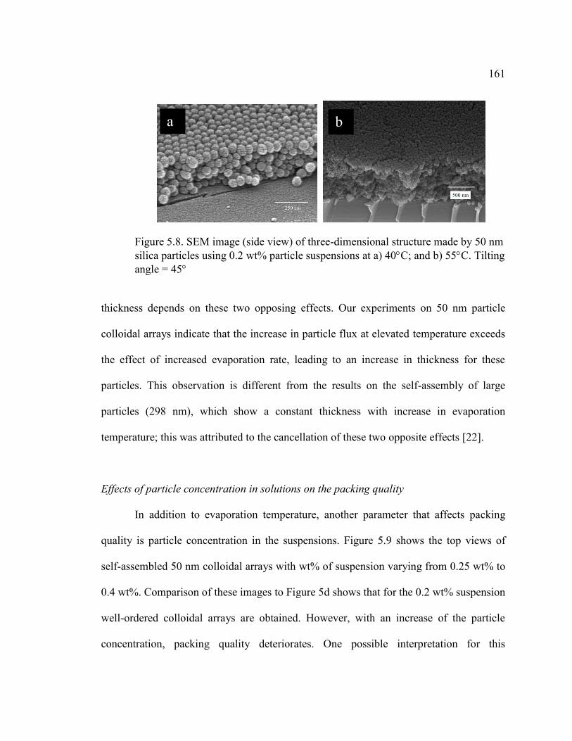
FIGURE 5.8 SEM image (side view) of three-dimensional structure
made by 50 nm silica particles using 0.2 wt% particle
suspensions at a) 40C; and b) 55C. Tilting angle = 45 .....................161
FIGURE 5.9 SEM image (top view) of three-dimensional structures
made by 50 nm silica particle samples using different
concentrations of silica particle suspensions a) 0.25 wt%;
b) 0.3 wt%; c) 0.4 wt% ..........................................................................163
FIGURE 5.10 SEM images of monolayer structures formed by 0.05 wt%
38 nm particles (sample 6 in Table 4.1) in ethanol.
a) image over 80m 60 m; b) image over 5m 3.7 m;
c) top view image over 2 m 1.5 m;
d) image over 1 m 0.7 m ................................................................165
FIGURE 5.11 Formation of ordered monolayer by horizontal evaporation with
concave meniscus formed in a container with walls ..............................168
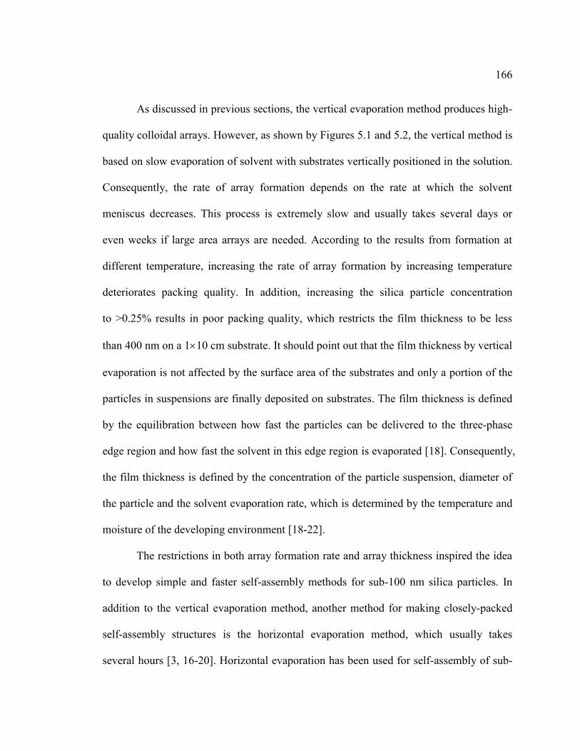
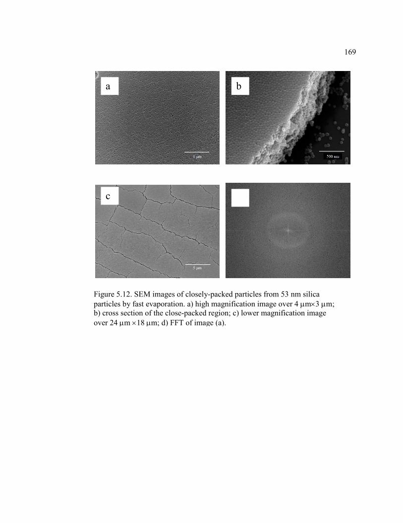
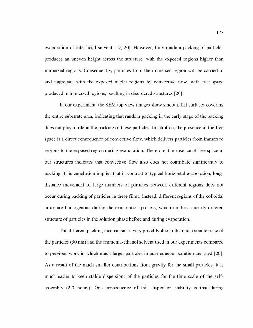
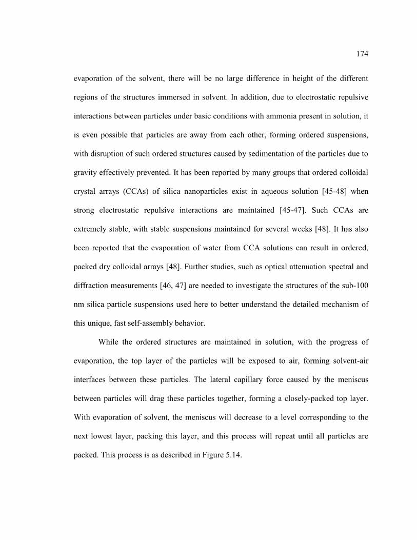
FIGURE 5.12 SEM images of closely-packed particles from 53 nm silica particles
by fast evaporation. a) high magnification image over 4 m3 m;
b) cross section of the close-packed region;
c) lower magnification image over 24 m 18 m;
d) FFT of image (a) ................................................................................169
FIGURE 5.13 SEM images of particle arrays from 53 nm silica particles by the fast
self-assembly method. a) top view; b) side view;
c) low magnification image over 3mm2mm ........................................172
FIGURE 5.14 Proposed self-assembly mechanism for sub-100 nm particles
by horizontal evaporation ......................................................................176
FIGURE 5.15 Proposed bridging mechanism for enhanced attractive interactions
between particles by ammonium [23, 49] ..............................................177
FIGURE 6.1 The ATR-FTIR set up for molecular diffusion measurement ................187
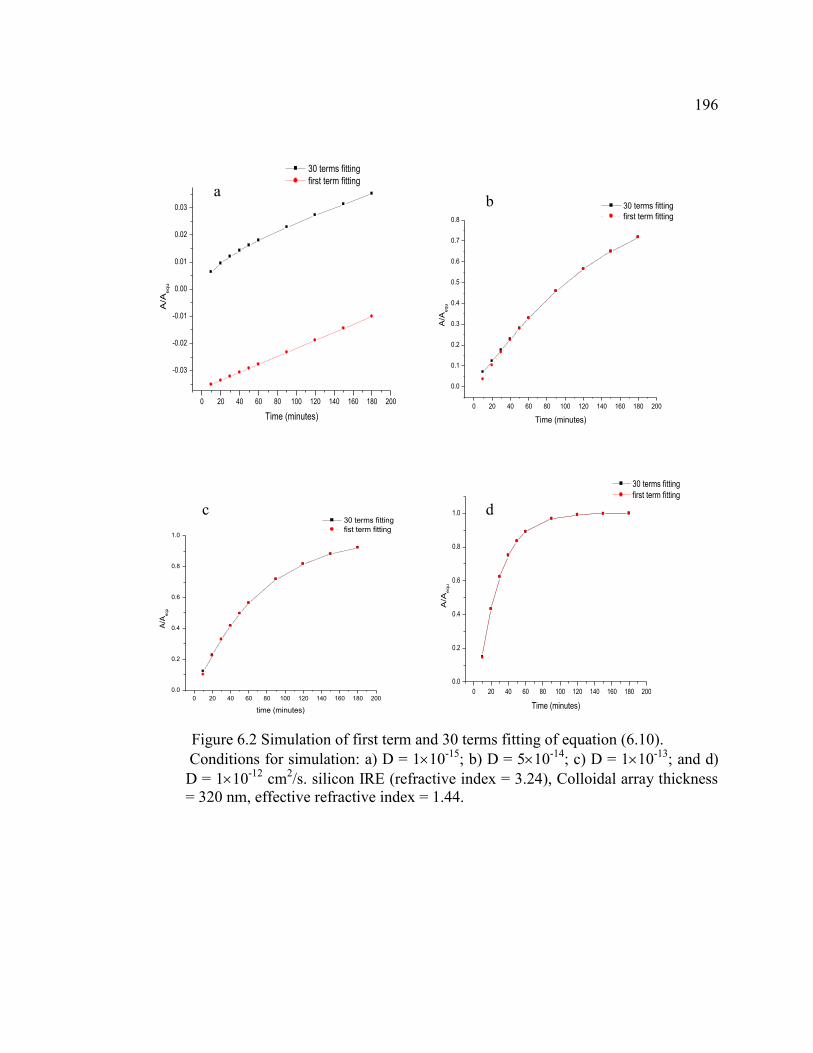
FIGURE 6.2 Simulation of first term and 30 terms fitting of equation (6.10).
Conditions for simulation: (a) D = 110-15
; (b) D = 510-14
;
(c) D = 110-13
; and (d) D = 110-12
cm2/s. silicon IRE
14
LIST OF FIGURES – Continued
(refractive index = 3.24), Colloidal array thickness = 320 nm,
effective refractive index = 1.44 ............................................................196
FIGURE 6.3 Kinetic spectra of hexane in colloidal array made of 50 nm particles
pre-filled by methylene chloride. Collection times are
11, 22, 39, 49, 56, 86, 101, 120 minutes, respectively, from
the bottom to the top. Resolution: 4 cm-1
, 500 scans.
Integration time: 5 min, Gain: 1, Reference: colloidal array
pre-filled with methylene chloride .........................................................198
FIGURE 6.4 Pore structures with big pores and defects .............................................199
FIGURE 6.5 ATR-FTIR signal versus diffusion time in colloidal array
made of 50 nm particles pre-filled by methylene chloride.
a) hexane, solid line is fit to A/Aequ = 1- exp (-0.01195t),
R2 = 0.99736,
2 = 0.00024; b) hexadecane,
solid line is fit to A/Aequ = 1- exp (-0.01108t),
R2 = 0.9908,
2 = 0.00004 .....................................................................200
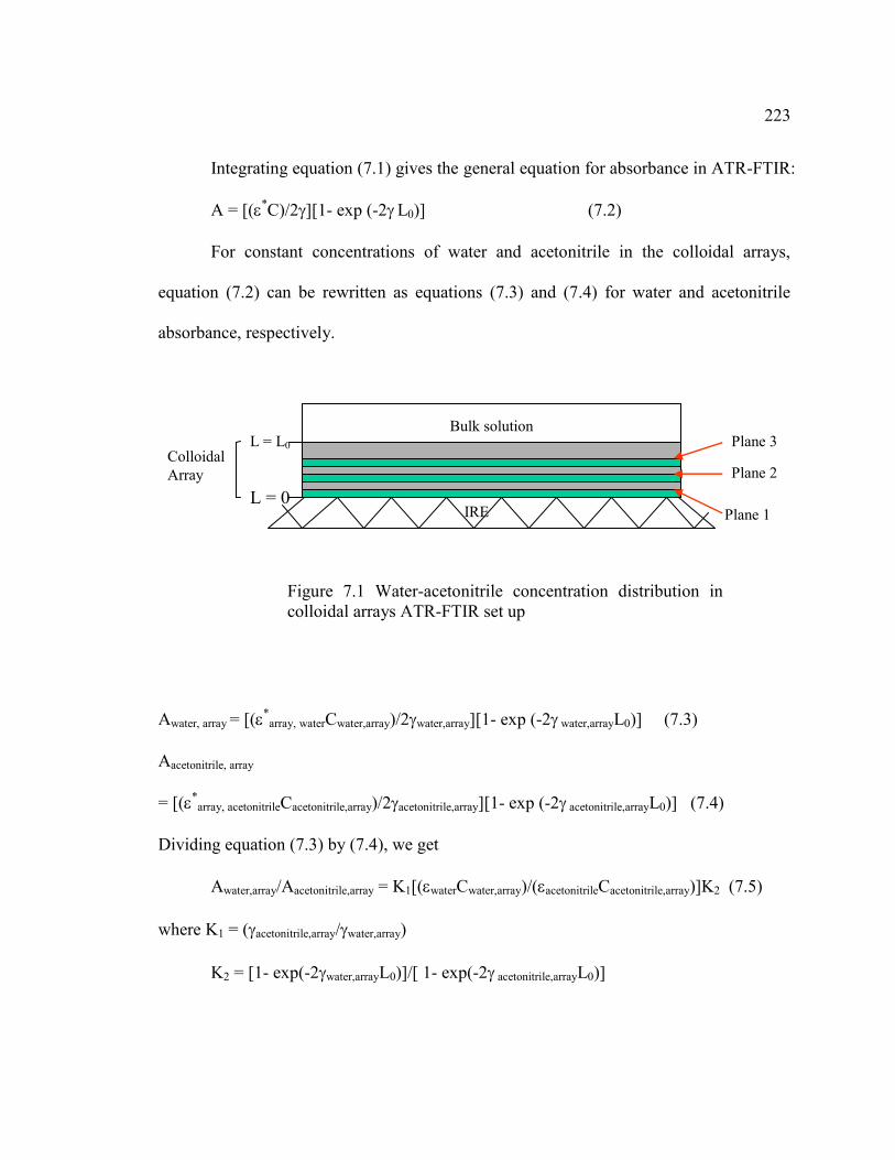
FIGURE 7.1 Water-acetonitrile concentration distribution in
colloidal arrays ATR-FTIR set up .........................................................223
FIGURE 7.2 Mole fraction of acetonitrile in pores of colloidal array
versus the corresponding mole fraction in bulk
solution using one-phase model .............................................................229
FIGURE 7.3 Evanescent wave penetrating into the bulk solution ..............................230
FIGURE 7.4 Experiment set up for measuring bulk solution absorbance using empty
colloidal array without being filled with solvents..................................232
FIGURE 7.5 Adsorption by colloidal array and bulk solutions...................................232
FIGURE 7.6 Mole fraction of acetonitrile in pores of colloidal array versus bulk
calculated using two-phase model .........................................................238
FIGURE A.1 Top and cross section images of colloidal arrays deposited on
commercial gold surface pre-coated with a 5 nm silica layer.
SEM conditions see Chapter 2 for top view and side view imaging .....271
FIGURE A.2 Nitrogen adsorption-desorption curves ..................................................273
15
LIST OF FIGURES – Continued
FIGURE A.3 BET equation of adsorption and desorption for curve 1 ........................275
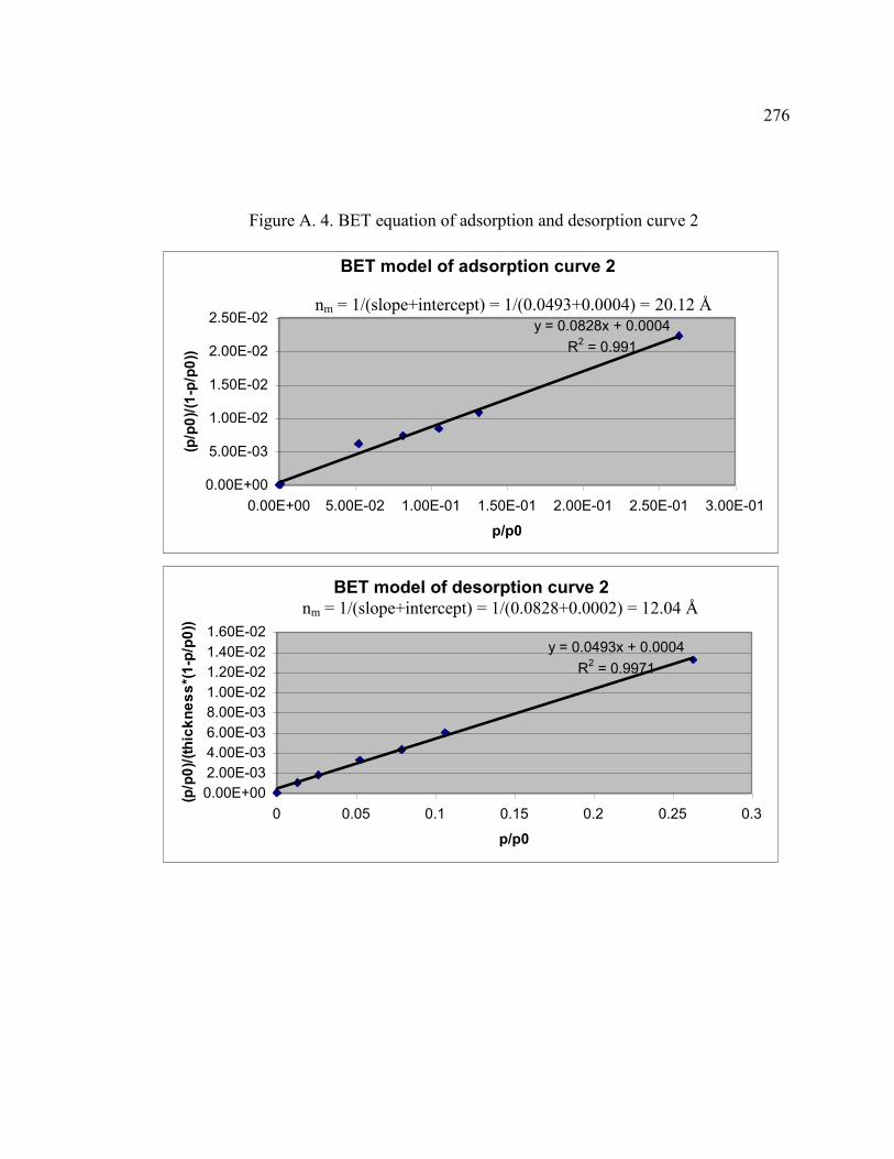
FIGURE A.4 BET equation of adsorption and desorption for curve 2 ........................276
FIGURE A.5 BET equation of adsorption and desorption for curve 3 ........................277
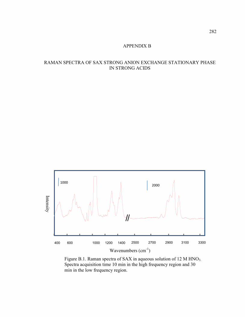
FIGURE B.1 Raman spectra of SAX in aqueous solution of 12 M HNO3
. Spectral acquisition times are 10 min in the high frequency region and
30 min in the low frequency region .......................................................282
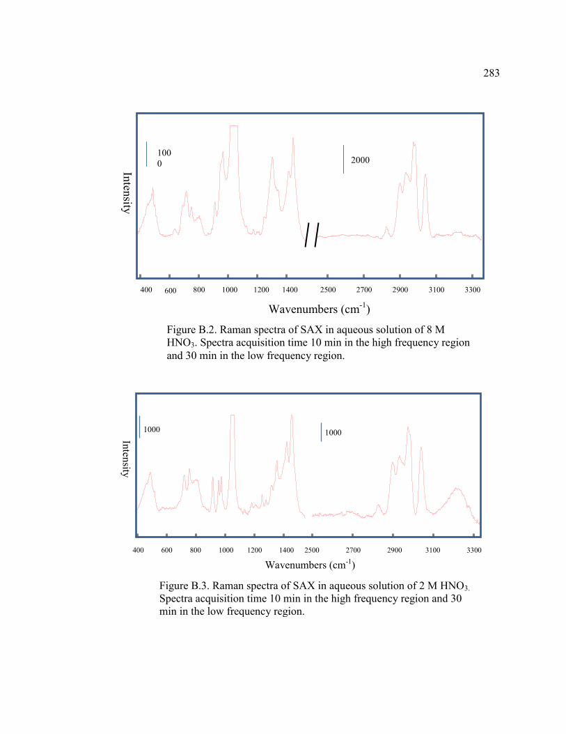
FIGURE B.2 Raman spectra of SAX in aqueous solution of 8 M HNO3
. Spectral acquisition times are 10 min in the high frequency region and
30 min in the low frequency region .......................................................283
FIGURE B.3 Raman spectra of SAX in aqueous solution of 2 M HNO3
. Spectral acquisition times are 10 min in the high frequency region and
30 min in the low frequency region .......................................................283
FIGURE B.4 Raman spectra of SAX in aqueous solution of 1 M HNO3
. Spectral acquisition times are 10 min in the high frequency region and
30 min in the low frequency region .......................................................284
FIGURE B.5 Raman spectra of SAX in aqueous solution of 0.1 M HNO3
. Spectral acquisition times are 10 min in the high frequency region and
30 min in the low frequency region .......................................................284
FIGURE B.6 Raman spectra of SAX in aqueous solution of 0.01 M HNO3
. Spectral acquisition times are 10 min in the high frequency region and
30 min in the low frequency region .......................................................285
FIGURE B.7 Raman spectra of SAX in aqueous solution of 12 M HCl
Spectral acquisition times are 10 min in the high frequency region and
30 min in the low frequency region .......................................................285
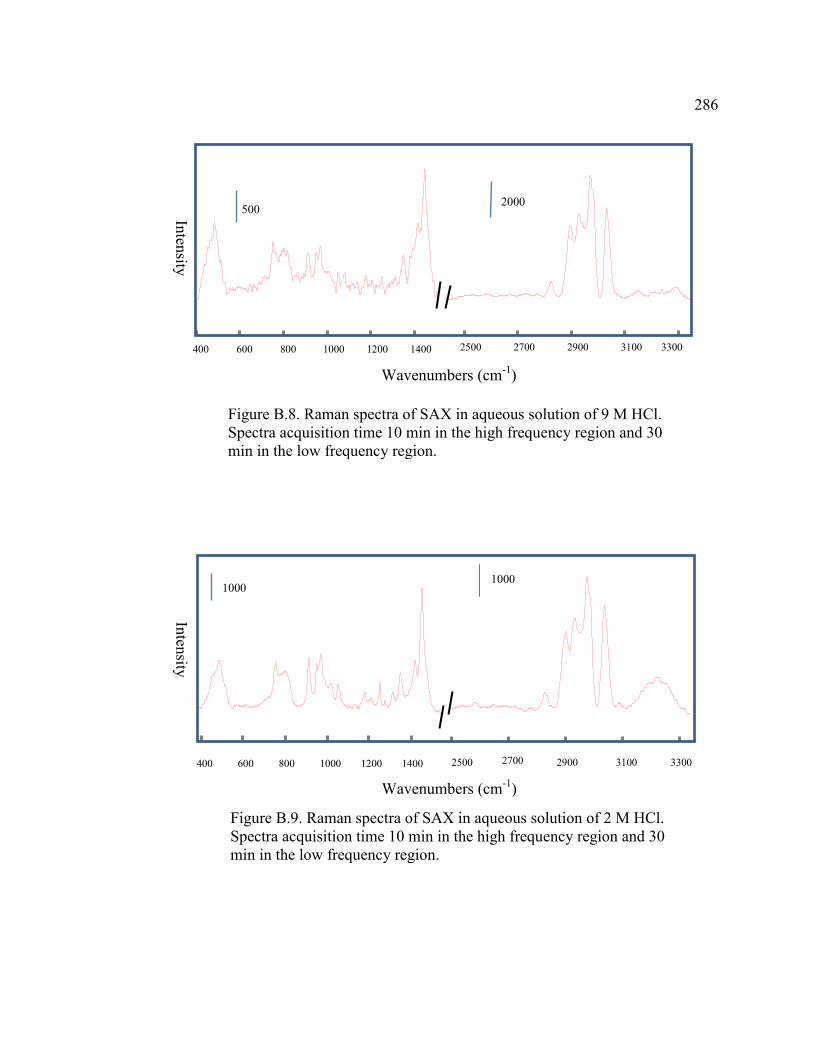
FIGURE B.8 Raman spectra of SAX in aqueous solution of 9 M HCl . Spectral acquisition times are 10 min in the high frequency region and
30 min in the low frequency region .......................................................286
FIGURE B.9 Raman spectra of SAX in aqueous solution of 2 M HCl . Spectral acquisition times are 10 min in the high frequency region and
30 min in the low frequency region ...................................................... 286
16
LIST OF FIGURES – Continued
FIGURE B.10 Raman spectra of SAX in aqueous solution of 1 M HCl . Spectral acquisition times are 10 min in the high frequency region and
30 min in the low frequency region ........................................................287
FIGURE B.11 Raman spectra of SAX in aqueous solution of 0.1 M HCl
. Spectral acquisition times are 10 min in the high frequency region and
30 min in the low frequency region .......................................................287
FIGURE B.12 Raman spectra of SAX in aqueous solution of 0.01 M HCl . Spectral acquisition times are 10 min in the high frequency region and
30 min in the low frequency region .......................................................288
17
LIST OF TABLES
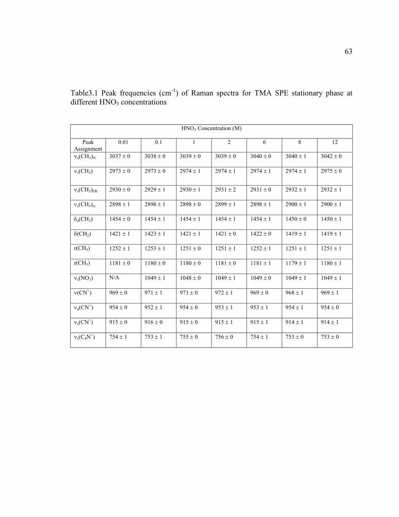
TABLE 3.1 Peak frequencies (cm-1
) of Raman spectra for
TMA SPE stationary phase at different
HNO3 concentrations ...............................................................................63
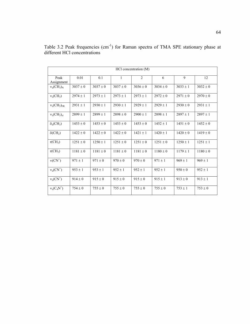
TABLE 3.2 Peak frequencies (cm-1
) of Raman spectra for
TMA SPE stationary phase at different
HNO3 concentrations ...............................................................................64
TABLE 3.3 Molar ratio of water to HNO3 and % HNO3 dissociation for
different HNO3 concentrations ................................................................80
TABLE 4.1 Experimental conditions, silica particle size and relative
standard deviation ..................................................................................142
TABLE 6.1 Diffusion coefficients of molecules in bare silica nanopores ................210
TABLE A.1 The BJH algorithm Excel table .............................................................267
18
ABSTRACT
Current study of separation mechanism in chromatography heavily relies on the
measurement of macroscopic properties, such as retention time and peak width. This
dissertation describes the vibrational spectroscopy characterization of separation
processes.
Raman Spectroscopic characterization of a silica-based, strong anion exchange
stationary phase in concentrated aqueous solutions is presented. Spectral response of
stationary phase quaternary amine is closely related to changes in interaction between
counter anions and the amine functional groups as the result of anion hydration. The
molecular-level information obtained will provide useful guidance for control of
stationary phase selectivity.
To study the effects of stationary phase pore size on separations processes,
monodisperse silica particles in the sub-100 nm range are prepared and self-assembled to
well-ordered, three-dimensional colloidal arrays. A modified LaMer model is proposed
and demonstrated for optimization of reaction conditions that lead to uniform and
spherical silica particles. This approach greatly reduces the number of training
experiments required for optimization. Fast Fourier transformation of colloidal array
scanning electron microscopy images indicates closely-packed hexagonal packing
patterns.
Using these arrays, a novel system for the measurement of molecular diffusion
coefficients in nanopores is reported. This system consists of an ordered colloidal array
with well-defined pore structure deposited onto an internal reflection element for in-sit
19
collection of kinetic information by attenuated total reflection-Fourier transform infrared
spectroscopy (ATR-FTIR). A mathematical model is established to extract diffusion
coefficients from these data. A decrease of approximately eight orders of magnitude in
molecular diffusion coefficients is observed for molecular transport in nanopores.
Finally, by using this colloidal array-ATR-FTIR system and the corresponding
mathematical models that describe absorption in the colloidal array, the distribution in the
nanopores of the acetonitrile organic modifier in an aqueous mobile phase solvent system
is determined. Based on the results of 50 nm colloidal arrays, pore surface properties
have a strong effect on the distribution of organic molecules from bulk solution to the
pores.
20
CHAPTER 1
APPLICATION OF VIBRATIONAL SPECTROSCOPY IN THE INVESTIGATION
OF INTERACTIONS AND DIFFUSION PROCESSES IN CHROMATOGRAPHY
Thermodynamic processes in column chromatography
Chromatography is one of the most important methods for the separation of
complex mixtures, both for purification and analytical aims [1]. One important driving
force for the separation process is the intermolecular interactions occurring in the
chromatography system, namely, the interactions between stationary phase and mobile
phase molecules, the interactions between solute and mobile phase molecules, and the
interactions between the solute and stationary phase [1, 2].
The consequence of different interactions in chromatography is that different
components in a mixture injected to the system will be eluted from the system with
different retention times. If we don’t consider the band broadening effects caused by the
kinetic processes (dynamics) in the system, which will be discussed in detail below, an
efficient separation system should be able to separate components (analyte) in the sample
with sufficient differences in retention times. This difference is evaluated by the
separation factor, , defined as [1]
analyte, matrix= tr, analyte / tr,
matrix = Kanalyte / K matrix (1.1)
where analyte, matrix defines the separation factor between the analyte and matrix molecules.
In equation (1.1), tr, analyte and tr,
matrix are the adjusted retention times of the matrix
21
components, respectively. Kanalyte and K matrix are the distribution coefficients of analyte
and matrix molecules between stationary phase and mobile phase, respectively. When
analyte, matrix equals unity, the analyte and matrix components will be co-eluted from the
column. A good separation is characterized by a value of analyte, matrix much bigger or
smaller than 1. The distribution coefficient, K, is defined as:
Ki = (CiS/ Ci
M)eq = exp (-i
0/RT) (1.2)
where Ki is the distribution coefficient of component i between stationary phase and
mobile phase, CiS and Ci
M are the equilibrium concentrations of i in stationary phase and
mobile phase, respectively, R is the gas constant and T is the temperature. -i is the free
energy change during the process of bringing the solute molecules from the mobile phase
to the stationary phase, which is defined as:
-i0 = i
S - i
M (1.3)
where iS and i
M are the standard chemical potentials of component i in stationary phase
and mobile phase, respectively and
i0 = Hi
0 – T Si
0 (1.4)
where Hi0 and Si
0 are the partial molar enthalpy and entropy under standard conditions,
respectively [1].
Combining equations (1.1), (1.2), (1.3) and (1.4) gives
analyte, matrix = exp (-analyte0/RT) / exp(-matrix
0/RT)
= exp ((matrix0 -analyte
0) / RT)
= exp{[(Hmatrix0 -Hanalyte
0 ) – T (Smatrix
0 - Sanalyte
0) / RT} (1.5).
22
Equation (1.5) indicates that the separation factor is governed by two separate terms: the
enthalpy term and entropy term.
The enthalpy term is most often controlled by intermolecular interactions between
the solute (analyte or matrix molecular) and the two phases (stationary phase and mobile
phase) that solute occupies [1]. A negative Hsolute0 corresponds to stronger
intermolecular attractions between the solute and stationary phase than between the
solute and mobile phase. From the enthalpy term, the bigger the difference in the net
interactions between matrix and analyte in the two phases, the better the separation
between the analyte and matrix components will be obtained.
Examples of accomplishing separation by entropy include those based on size
exclusion mechanisms [1], including gel permeation chromatography, gel filtration
chromatography [3-5], capillary SDS gel electrophoresis [6-9], and SDS electrophoresis
[10]. In these separation systems, the mobile phase acts more like a carrier for analyte
and matrix components without any specific interactions between these components and
the mobile phase, and similarly, the interactions between stationary phases and the
analyte and matrix components are deliberately made very weak [5, 11, 12]. The
separation is accomplished by how well the molecules can fit into the pores of the
stationary phase. Consequently, the enthalpy item in equation (1.5) is ignored and
equation (1.5) becomes:
analyte, matrix = exp{[- T (Smatrix0 - Sanalyte
0) / RT} (1.6)
When bigger molecules approach the stationary phase, they have to arrange their
positions and orientations to slip into the pores of the stationary phase, which is a process
23
leading to more ordered arrangements, costing a decrease in entropy (S0 <0), while for
smaller molecules, the entropy decrease is smaller [13, 14]. Consequently, molecules are
separated due to their different sizes, with smaller molecules eluted later than bigger ones.
Equation (1.5) provides the general thermodynamic foundation for the separation
process between the analyte and matrix molecules. However, it doesn’t relate retention
and separation factor of a system to any particular physical properties of the solute,
stationary phase or mobile phase in the system. Due to the fact that different separation
modes are mainly based on different types of interactions and correspondingly, different
thermodynamic processes describing these interactions, separation models corresponding
to different separation modes have been developed. We will discuss the separation
models for ion exchange and reverse phase chromatography in the following sections.
Ion-stationary phase interactions in ion chromatography: Stationary phase selectivity
In ion chromatography, the separation factor is called the selectivity coefficient. It
has been widely used in ion chromatography to evaluate how efficiently an ion exchange
system can separate a specific pair of ions [15].
The selectivity coefficient reflects the relative affinity of ions to the stationary
phase. In ion exchange chromatography, electrostatic interactions exist between counter
ions and the charged functional groups on the stationary phase possessing opposite
charges to those of counter ions. Electrostatic interactions between the counter ions and
stationary phase are proportional to the charges of the ions and inversely to the distance
between the ions and the functional group. Therefore, these interactions depend on the
24
charge/size ratios of the counter ions, and the electrostatic interactions between the
counter ions and stationary phase are different, which is the major thermodynamic
driving force for separation in ion exchange chromatography. Ions strongly interacting
with stationary phases will have longer retention times than those interacting more
weakly [15].
One strategy to change the selectivity of an ion exchange system is to attach extra
chemical species in addition to ion exchange functional groups to the stationary phases.
These extra chemical species have specific interactions with some ions. Consequently,
retention times of the ions having such specific interactions with stationary phases
increase while other ions in the samples are not affected. Crown ethers, for example, have
been used for the separation and purification of metal ions due to the fact that metal ions
with appropriate sizes will form stable complexes with the particular crown ether
functional groups attached to the stationary phases, and therefore, have a longer retention
time than other metals [16-21].
Another strategy to change the selectivity that has been widely practiced is by
changing the hydrophilicity of the stationary phases [22-24]. This can be accomplished
either by introducing hydrophilic functional groups to the stationary phases [23, 24] or
changing the cross-linking of the stationary phases [15, 23]. Pohl et al. [24] compared
four anion exchange quaternary ammine functional groups with different hydrophilicities.
Results show that the more hydrophilic the functional groups are, the stronger the
retention of counter ions with higher hydration enthalpies. On the more hydrophilic resins,
hydroxide was found to be effective at displacing ions, but much less so on the more
25
hydrophobic ones. This discovery leads to a series of hydrophilic ion exchange stationary
phases using hydroxide as the eluent ion. The advantages of using hydroxide as the eluent
in ion chromatography includes the following: first, when passing the suppressor,
hydroxide ions are converted to water, which has very low background conductivity and
thus, provides good signal-to-noise ratio for conductivity detection of ions [15]. Second,
hydroxide can be produced automatically by electro-hydrolysis of water and the
concentrations of the hydroxide thus produced can be accurately controlled, which not
only eliminates the possibility of reagent contamination during the preparation of eluents,
but also improves the automation of the operation [25].
On the other side of the spectrum, however, bulky and highly polarizable anions
are found to be strongly retained on stationary phases containing hydrophobic functional
groups, which usually leads to very long retention times, causing problems of low
detection sensitivities and asymmetric peaks [15, 26-29]. Jackson et al. [26] compared the
elution of perchlorate anion on two columns with different hydrophilicities. Results show
that on the more hydrophilic column, perchlorate was eluted in 10 min while on the more
hydrophobic column, organic modifier, such as cyanophenate had to be added in order to
elute perchlorate out of the column. An “ultra-low hydrophobic” column that was
reported for the analysis of perchlorate with reasonable analysis time consists of low
cross-link (1%) functional groups containing hydrophilic hydroxyl functional groups [28].
Although manipulating the hydrophilicity of stationary phases is a powerful
strategy in controlling selectivity, the fundamental chemistry of such a strategy is still not
clear. Reichenberg proposed [15] a model to describe the selectivity in ion
26
chromatography by considering the net free energy change in removing ion M from
solution and exchanging it for ion N on the functional group, which can be expressed as:
GM/N = [e2 / (rA + rN) – e
2 / (rA + rM) – (GN - GM)
(1.7)
where GN and GM are the standard free energies of hydration of the respective ions, e
is the electronic charge, rA is the radius of the functional group, and rN and rM are the radii
of ions M and N, respectively. The first term on the right side of the equation refers to the
contribution from electrostatic interactions between counter ions and stationary phases
during the ion exchange process, while the second term refers to the free energy change
corresponding to the loss or rearrangement of the hydration layers of the ions when these
ions approach and interact with the functional groups on the stationary phase.
Although thermodynamically reliable, the model doesn’t consider the fact that
instead of bare ions without any water molecules in their hydration layers, the counter
ions may interact with the stationary phases as partially hydrated ions, with some of the
water molecules still remaining in their hydration layers. Therefore, a more accurate
description for the free energy change during an ion exchange process should define rA,
rN and rM in equation (1.7) as the radius of the exact forms of the functional group and
counter ions interacting in the particular ion exchange system under the investigation.
Similarly, GN and GM should be defined as the exact free energy changes of the
respective ions during the process of rearranging the hydration layers, rather than the
standard free energies of hydration of these ions. Consequently, accurate and reliable
molecular level information, such as how the hydration layer of an ion changes when
27
approaching the stationary phases, and how the hydrophilicity of a stationary phase
affects such change, is essential in defining the parameters in equation (1.7) for accurate
estimation of selectivity for an ion exchange system.
Recently, X-ray absorption fine structure (XAFS) and neutron diffraction method
have been intensively used to study the structure of ion exchange systems [30-38].
Results on chloride show that the hydration layer structure of chloride is a function of the
availability of water molecules in the environment. In addition, different hydrated species
of ions coexist in the stationary phase, with their ratios changing depending on the
hydration environment. The fine structures of how ions interact with the stationary phase,
as well as how the hydration environment affects the structure between the counter ions
and stationary phase, provides important molecular level information for understanding
selectivity in ion exchange. However, vibrational spectroscopy techniques that can
provide direct and straightforward information on the interactions between counter ions
and stationary phase in aqueous solutions that mimic real separation conditions have not
yet been reported.
Retention models in reversed phase liquid chromatography
Reversed phase liquid chromatography (RPLC) is one of the most important
chromatography techniques [39]. It is estimated that 60%-80% of analytical separations
are carried out by RPLC1.2
. Separation mechanisms for RPLC have been studied for more
than 30 years. The solvophobic [2, 40, 41] and partition models [42, 43] are the two
major models used to describe the separation process in RPLC. Since both models are
28
derived using complicated mathematics and statistic thermodynamics calculations, a
concise review of the basic premises and logic on which the two models are established
will be useful for discussion of these models without being distracted by the complicated
mathematics.
Solvophobic model
The solvophobic model is based on the idea that the entropy-driven hydrophobic
interaction is the major interaction responsible for retention and separation in RPLC [2,
39-41]. According to the solvophobic model proposed by Horvath et al. [2, 40, 41],
retention of a nonpolar solute molecule, S, on a stationary phase modified by functional
group L, consists of the following processes: (1) association of SL at the interface
between mobile and stationary phases; (2) creation of a cavity in the mobile phase for the
associated SL; (3) close of the cavities in the mobile phase which used to be occupied by
the solute molecules S before retention; (4) close of the cavities in the mobile phase
which used to be occupied by the functional group L at the interface of the mobile and
stationary phases before retention; (5) entropy change during the process of the retention.
The total free energy change corresponding to the retention of solute is therefore the sum
of the free energy changes corresponding to these five processes.
The solvophobic model considers the stationary phase as a surface where the
association between solute and functional group occurs at the interface between
stationary phase and mobile phase [2]. The retention of solute mainly depends on the free
energy change for cavity creation and destruction in mobile phase, which is strongly
29
affected by the surface tension of the mobile phase and the size of the solute species [2].
The solvophobic model can explain some retention phenomena in RPLC, such as the
linear relationship between capacity factor and surface tension of the mobile phase [2, 44],
and the linear relationship between capacity factor and solute size [2, 39-41, 45-49].
Partition model
Different from the solvophobic model in which the stationary phase is considered
as a surface providing the interface for the retention of solute to occur, the partition
model considers the stationary phase as a “liquid” or semicrystal into which the solute
can diffuse [42]. According to this model, the distribution coefficient of solute is the
same as that in the corresponding bulk oil/water system, since the thermodynamic
processes involved in these two systems that define the distribution of a solute between
the two phases are the same.
The interphase partition model was developed by Dill [42, 43]. The interphase
partition treats the stationary phase as consisting of a set of horizontal and parallel planar
layers of interphase, starting from the interface between the silica and the grafted alkyl
chains on the silica, to the free ends of the alkyl chains that contact the mobile phase.
Solute molecules diffuse easily into the layers closer to the free end of the alkyl chain,
but it is more and more difficult for diffusion into the layers further away from the mobile
phase-stationary phase interface. This is because the insertion of solute into the
interphase causes an increase in volume of the interphase. When the chains are restricted
on the silica surface, the chains have to extend to accommodate the space for solute. The
30
consequence of such chain extension is an increase in the alignment of the chains along
the axis normal to the silica-alkyl chain interface, which leads to a decrease in the
configurational entropy of the grafted chains. Such an entropy decrease process disfavors
retention of the solute [42].
Assuming that the stationary phase consists of L interphase layers and the total
sites in each layer for the occupation of solute is N0, due to the configurational entropy
restriction, the real number of sites available for occupation in a particular layer i is then
Ni = N0 qi (1.8)
where qi is a statistic weight with a value between 0 and 1 [42] that accounts for the
effects of the conformational entropy of restrained chains on the uptake of solute. The
total sites for occupation of solute in the whole stationary phase is then
Ns = N0 (qi) (1.9)
The “effective” phase ratio, which is the ratio of the volumes that are available for the
occupation of solute in stationary phase and mobile phase, respectively, is then
= (NsVs) / (NVs) = Ns / N = (N0 (qi)) / N (1.10)
where Vs is the volume of the solute molecule.
In a bulk water/oil system, there is no configurational restraint, so qi = 1 for all
layers; therefore, bulk = (N0L)/N, and the capacity factor is:
kbulk = K bulk = (K N0 L) / N (1.11)
where K is the distribution coefficient of the solute between the stationary and mobile
phases. In RPLC, as mentioned above, the distribution coefficient is the same as in bulk
water/oil system in partition models, and therefore,
31
kRPLC = K = (K N0 (qi)) / N (1.12)
Dividing equation (1.12) by (1.11) and rearranging, we get
kRPLC = [(qi) / L] kbulk (1.13)
In RPLC, due to the configuration constraint, the value of (qi) will always be smaller
than L. Consequently, equation (1.13) predicts that the peak capacity of a specific solute
in RPLC will always be smaller than in the corresponding bulk water/oil system.
In addition, provided that the interphase ordering is little affected by the solute,
the values of qi and L are constants for a given RPLC system [42]. Using equation (1.13),
we can evaluate the selectivity factor of two solutes, a and b, as follows:
RPLC, a, b = kRPLC,a / kRPLC,b = kbulk,a / kbulk,b = bulk, a, b (1.14)
Equation (1.14) predicts that for a specific solute pair, selectivity in RPLC should be the
same as in the corresponding oil/water systems. All these predictions are consistent with
the experimental results [50-52].
According to equation (1.13) and equation (1.11), the logarithm of ln kRPLC can be
defined as:
lnkRPLC = ln [(qi) / L] + ln kbulk
= ln [(qi) / L] + ln [(KN0L) / N] = ln [(qi)N0 / N + ln K (1.15)
For given RPLC and oil/water systems, the values of qi, L and N0 are determined by the
alkyl chain structure, and therefore, are constant. N is also a constant defined by the total
volume and property of the oil phase. Consequently, equation (1.15) predicts that for a
specific solute, there is a linear correlation between the logarithm of the peak capacity in
RPLC system and the logarithm of its distribution coefficient in the corresponding
32
water/oil bulk system, with a slope of 1, which has been observed in a variety of
experiments [53-59].
Comparison of solvophobic model and partition model
The solvophobic model emphasizes the role of hydrophobic effects on retention
of the solute. When nonpolar solute molecules are introduced into an aqueous
environment, due to the weak interactions between solute and water molecules, cavities
must be created to accommodate the uptake of these nonpolar molecules. However, the
formation of solute-containing cavities with water molecules surrounding these cavities is
a large negative entropy process [60]. Consequently, to overcome the loss in entropy,
non-polar segments of molecules will favor removal from the aqueous medium and /or
will tend to group together [39]. Hydrophobic effect is not caused by any interactions
between nonpolar species. It is more a solvent effect. It requires a network formed by a
large number of water molecules through hydrogen bonding that can effectively expel the
intrusive nonpolar species from such a network.
According to the solvophobic model, retention of solutes occurs in the interfacial
region between the mobile and stationary phases. In this region, a large number of water
molecules are available, leading to a strong hydrophobic effect in this region. According
to the partition model, the solute molecules can freely penetrate into the stationary phase.
On one hand, it increases the contribution of partition to the retention. On the other hand,
due to the hydrophobic property of the stationary phase, only a small number of water
molecules are available in the internal structure of the stationary phase. Furthermore, the
33
water molecules in the stationary phase are “cut” into small separate pools and capillaries
by the alkyl chains in the stationary phase, and thus, can not effectively form strong
network to expel solutes, which leads to a weak hydrophobic effect. Consequently, the
partition mechanism will be the major contributor to the retention.
Since the solvophobic model treats the stationary phase as a surface and the
retention of the solute is restricted to the interfacial region between the mobile and
stationary phases, the structure of the stationary phase alkyl chains should not affect
distribution of the solute and the retention of solute should be more affected by the
mobile phase. According to the partition mechanism, the solute will penetrate into the
stationary phase structure for retention, and therefore, the stationary phase structure, such
as the surface coverage and alkyl chain length, will affect distribution of the solute, which
is supported by experimental evidence [43, 61].
Although the partition mechanism can explain much retention behavior in RPLC,
it has been demonstrated that for some amphiphilic organic polymers such as PEO [62,
63], the entropy contribution dominates retention, indicating a strong hydrophobic effect
on the retention, which is consistent with the solvophobic model. In addition, theoretical
studies of separation mechanisms in RPLC, especially thermodynamic studies, still
heavily rely on the adsorption mechanism [64-66]
and hydrophobic effects [67].
Furthermore, it has been reported that depending on molecular size, molecules may not
completely insert into the stationary phase [68-70], which may cause retention that does
not purely rely on partitioning.
34
Up to now, no universal model has been developed to explain and predict
retention in RPLC, as discovered in some systems in which factors other than partitioning
and hydrophobic effects play important roles in retention and selectivity [71, 72]. From
chronology, the solvophobic model was developed earlier and is based on
thermodynamic principles and derivation, while the partitioning model includes a more
molecular-level picture of RPLC systems. The development trend of these models
demonstrates that fundamental study of RPLC systems at the molecular-level greatly
impacts this field. For example, molecular-level information of how the grafted chain
conformation changes with separation conditions such as temperature has been reported
as the major reason for the great kinetic changes of molecular mass transfer in stationary
phases [68]. The chain conformation and cavities formed between the grafted alkyl
chains of the stationary phase are the major reasons for shape selectivity for high surface
coverage stationary phases with long alkyl chains [71, 72].
Mobile phase composition
One topic important to the establishment of the RPLC retention model is the
effect of mobile phase composition on retention. Both the solvophobic and partitioning
models assume that the mobile phase passing through the surface of the stationary phase
always has the same composition as the exterior mobile phase. However, it has been
observed that depending on the properties of the organic components, the aqueous-
organic mobile phases interacting with the stationary phase, either in the interfacial
region between the two phases or in the stationary phase, have different compositions
35
from the bulk mobile phase. Organic modifiers have always been observed to be enriched
in/on the stationary phase [63-66, 73-76]. This composition difference is attributed to
stronger interactions between the organic modifiers and the stationary phase compared to
those between water and the stationary phase. Karger et al. [66] observed that the amount
of organic modifiers partitioned in the stationary phase first increases with the percentage
of the organic modifiers in the aqueous mobile phase until arriving at a maximum, and
then starts to decrease. These authors attributed this behavior to the hydrophobic effect of
the aqueous mobile phases [67]. On one hand, with the increase of the organic modifier
concentration in the mobile phase, more organic modifier will be distributed in the
stationary phase. On the other hand, with the increase of the organic composition in the
mobile phase, the hydrophobic effect decreases and thus, results in less organic modifier
being repelled by the mobile phase to the stationary phase. The net results of these two
opposite effects on the uptake of organic modifier to the stationary phase versus the
mobile phase organic modifier concentration lead to the maximum uptake of the organic
modifier [67].
Porous silica particles are the most commonly used stationary phase materials due
to the high column capacity provided by these materials, which is especially useful for
the analysis of complicated samples compared to nonporous particle stationary phases
[77-79]. Therefore, the effect of pores of these materials on mobile phase composition
cannot be ignored. Comparison pore volume measurements on RPLC porous stationary
phases using nitrogen and a variety of water-organic mobile phases including water-
methanol and water-acetonitrile show that these mobile phases can occupy the same pore
36
volumes as nitrogen does, meaning that all the pores can be occupied by the aqueous
mobile phase [80]. However, these measurements don’t provide detailed information
about how the different components of the mobile phase are distributed in the pores.
Molecular diffusion experiments in alkyl chain modified nanopores show that water and
organic molecules have different abilities to penetrate the small, hydrophobic and dry
pores [81-83]. Results based on 200 nm and 20 nm pores show that for these hydrophobic
nanopores, water molecules cannot penetrate the pores while nonionic species can
penetrate the pores by Langmuir adsorption based diffusion [81]. Based on these
observations, when the mobile phases in RPLC, which usually are the mixtures of water
and organic solvents, pass these pores, the composition of the solvents in the pores should
be different from that outside the pores unless the operation pressure of the RPLC
compresses water into the pores. Such observation raises a fundamental question
concerning the mobile phase composition in the stationary phases: in addition to the
stronger interaction between organic modifier and stationary phase and the hydrophobic
effect, is it possible that the difference in the pore permeability of water and organic
modifiers is also responsible for enrichment of the organic modifier in the stationary
phase? However, the composition of commonly used mobile phases in pores has not been
reported yet. To achieve this, model systems that can provide controllable pore size with
surface properties mimicking the commonly used silica substrates for RPLC stationary
phases will provide a useful platform for investigation of the effects of pore size, surface
hydrophobicity, grafted alkyl chain surface coverage, bulk mobile phase composition,
37
temperature and operation pressure on the distribution of water and organic modifiers of
mobile phases in pores.
Diffusion of molecules in chromatography columns: Dynamics in separation systems
The thermodynamic processes that occur in separation systems define the
retention times of the analyte, which define how well two components can be separated.
However, completely separating components in a mixture also requires that all molecules
of the same component have very close retention times, eluting as narrow peaks on the
chromatographs. Narrow peaks enable separation of two components even if the positions
of the peaks are close to each other. On the other hand, broad peaks not only lead to peak
overlap, but are also hard to detect quantitatively due to difficulties in distinguishing the
broad peaks from the baseline [1]. The separation of two components is usually evaluated
by resolution, which considers both peak position separation and peak width. Resolution
is defined as
Rs = (tr1 – tr
2) / wb (1.16)
where tr1 and tr
2 are the retention times of component 1 and 2, respectively, and wb is the
average base width of the two peaks [1].
When a sharp peak is injected into a separation system, the peak will experience
broadening during its movement along the flow channel in the separation medium. Peak
broadening is a function of both separation hardware and operating conditions, which is
usually evaluated by plate height, defined as [1]:
H = 2/L (1.17)
38
where 2 is called the variance. The square root of the variance, , called the standard
deviation, is usually used to measure the overall width of the chromatographic peaks. For
normal Gaussian peaks, is the distance from the peak center to the inflection point of
the peak. L is the path length of the medium used for separation. Equation (1.17) shows
that the broader the peaks, the higher the value of H. Therefore, small values of H are
characteristic of narrow peaks and high separation efficiency [1].
When the mobile phase flow rate, u, is relatively high, which is the case for most
RPLC operations, the plate height H is usually described by the Van Deemter equation [1,
84-86]:
H = A + B / u + C u (1.18)
Equation (1.18) describes the three major sources of peak broadening: (1) eddy diffusion,
which is expressed by the A term, is caused by the different flow streams that solute
molecules follow in the column. When mobile phase flows along the column, the flow is
separated into different flow streams or channels in the column due to the obstacle effect
of the stationary phase particles. As a result, solute molecules take different flow paths
through the packed column, depending on what flow streams they follow. Molecules
following wider flow paths move faster than those following narrower path. In addition,
different flow paths have different lengths. The differences that solute molecules
experience in both the flow rate and path length in the column result in spreading of the
narrow peak initially injected. In addition, diffusion of solute molecules between
channels with different flow rates also cause peak broadening, which is called mobile
39
phase mass transfer effect. Mobile phase mass transfer is usually coupled to eddy
diffusion item in the Van Deemter equation, as expressed by equation (1.19) [86].
A = 1 / [(1 / Hedd) + (1 / Hmobile-mass-transfer)] (1.19)
(2) longitudinal diffusion, as described by the B/u term, is caused by the diffusion of
solute molecules along the column axis due to solute concentration gradients existing
between the peak center and the ambient mobile phase environment. (3) mass transfer
process of solute molecules in the column. This item can be further separated into two
contributions: stagnant mobile phase mass transfer and stationary phase mass transfer,
described by Csm and Cs in equation (1.20), respectively [85].
C = Cs + Csm (1.20)
Mass transfer is caused by the slow diffusion of solute molecules in either
stagnant mobile phase or stationary phase. The stagnant mobile phase mass transfer has
strong effects on the plate height when porous stationary phases and big solute molecules,
such as polymers [87], steroids, peptides and proteins [79, 88-91], are involved in the
separation. In the column, flow rates in channels are proportional to the square of the
width of the channels [85, 86]. Therefore, mobile phase in the small intra-particle pores
with very narrow width will move very slowly or not at all, thus forming stagnant regions.
Solute molecules following flow paths through these stagnant regions can only move in
and out of these regions by diffusion, causing peak broadening [85, 92].
Stationary phase mass transfer is caused by slow adsorption/desorption kinetics of
solute molecules on the stationary phase surface when separation is based on adsorption.
For systems in which separation is based on partitioning, diffusion of the solute
40
molecules into and out of the stationary phase is the cause of stationary phase mass
transfer [1].
The contribution of A, B, Cs and Csm in equations (1.18)-(1.20) to plate height
have been derived as functions of the diameter of the stationary phase particles, dp,
mobile phase velocity u, and diffusion coefficients Dm and Ds of solute molecules in
mobile and stationary phases, respectively, as shown in equations (1.20-1.25) [85, 86]:
Hedd = 2 dp (1.21)
Hmobile-mass-transfer = Cmobile-mass-transfer dp2
u / Dm (1.22)
B = Dm (1.23)
Cs = Cstationary-mass-transfer dp2 / Ds (1.24)
Csm = Cstagnant-mass-transfer dp2 / Dm (1.25)
, , Cstationary-mass-transfer, and Cstagnant-mass-transfer are parameters related to the packing
structure of the column and capacity factor of the solute, which are constants for specific
solutes in a given separation system [86].
Effects of molecular diffusion on separation performance
In separation systems in which packed columns are used, plate height increases
with flow rate, especially for big solute molecules when porous particles are used as
stationary phases, making fast and efficient separations difficult. This is generally
attributed to the slow diffusivity of solute molecules in the intra-particle pores of the
stationary phase [79, 87-96] that gives rise to the stagnant mobile phase mass transfer
term, Csm, in equation (1.25) [79, 91-96]. According to equation (1.25), the stagnant
41
mobile phase mass transfer is proportional to the square of the distance required for
solute molecules to diffuse throughout the stagnant mobile phase. This diffusion distance
is proportional to the particle size. In addition, Csm is inversely proportional to the mobile
phase diffusion coefficient.
Several strategies and stationary phases have been developed to reduce stagnant
mobile phase mass transfer for fast and efficient separation of proteins and other bio-
molecules. One strategy is to use small porous particles, which decreases the diffusion
distance in the stagnant mobile phase [79, 93, 97, 98]. However, the ultrahigh pressure
required to drive the mobile phase through columns packed with small particles [77, 98-
100], as well as the difficulties in packing small particles into columns [77] limits wide
application of these stationary phases. In addition, the velocity surge of the mobile phase
caused by ultrahigh pressure may cause extra peak broadening [99] or conformation
change of the solute, which complicates the separation mechanism [100]. Nonporous and
pellicular stationary phases using a thin porous film outside the inert cores eliminates or
decreases the volume of the intra-particle pores for occupation of stagnant mobile phase.
As a result, the diffusion distance required for the stagnant mobile phase mass transfer
decreases, which either completely eliminates slow stagnant mobile phase mass transfer
or reduces the contribution of the stagnant mobile phase mass transfer to the plate height
[77, 94, 98, 101, 102]. The problem of this strategy is that these stationary phases usually
have small surface areas, which leads to small column capacity and thus, are easy to
overload and cannot be used for samples with complicated compositions [79, 93, 97, 98,
100]. Another strategy is to introduce big “through pores” to the stationary phases, as
42
demonstrated in perfusion and monolithic stationary phases [93, 95, 96, 103-106]. It is
generally believed that the convective flows in the through pores allow big solute
molecules to enter the short diffusive pores more readily, which increases the apparent
diffusion coefficients of solute molecules “lumping” the true diffusivity and convection
in the stagnant mobile phase [93].
Although playing an important role in the separation efficiency, fundamental
understanding of how solute molecules diffuse in pores of the RPLC stationary phase is
still not clear. Studies of molecule diffusion in nanopore structures indicate that the
diffusion coefficients of molecules are greatly affected by the size of the pores relative to
the molecule size [107-110] and the pore structure [111]. Depending on the pore structure
and molecule size, a decrease of two orders of magnitude [108] or more in diffusion
coefficients in pores compared to bulk has been observed [109]. In the stagnant mobile
phase restricted in the small intra-particle pores of the stationary phases, such a decrease
in diffusion coefficient might not only be responsible for peak broadening, but also for
the low recovery of big molecules such as peptides from the commonly used RPLC
stationary phases [112-113]. The low recovery of big peptide molecules from commonly
used RPLC stationary phases (pore size 20 nm) implies that very slow mass transfer that
lasts longer than the whole chromatographic run may occur in the pores of the stationary
phases, especially for big peptides (>10kD) [113]. In addition, since recovery has been
found to be greatly improved by increasing the intra-particle pore size [112, 113], it is
obvious that diffusion in the pores has a strong effect on recovery. However, since all
current methods for chromatographic kinetics study, including those based on
43
spectroscopy [114, 115] and peak profile analysis, only consider relatively fast kinetic
processes that can be finished within the time scale of one chromatographic run [68, 87-
90] or less [114, 115], fundamental study of such process has not been reported yet.
The study of diffusion of molecules in pores at the nanometer level, especially
how the pore size affects diffusion of molecules, is importance in the design of bio-
separation systems. Although pore size effects on plate height and mass transfer of solute
have been observed for a long time, the systematic study of how pore size affects
diffusion at the molecular level, and its possible effects on macroscopic separation
performance, has not been reported. In order to achieve this, model systems with
controllable pore size as well as the appropriate detection system that can collect kinetic
information about diffusion on time scales longer than the normal chromatographic run is
necessary.
Goals of this research
The goals of this work were twofold: (1) to obtain a molecular picture of
chromatographic systems using vibrational spectroscopy, with discussion of how this
molecular-level information will be useful for both thermodynamic and dynamic study of
separation, and (2) to provide novel strategies to extract molecular-level information from
systems mimicking separation systems in the real world. Due to the limited time the
author can spend on each project and the novelty of all of the projects, each strategy used
in this work still has much space for further development to extract more molecular-level
44
information in separation systems, which will be discussed in the future directions
chapter.
Specific goals of this work included:
1. Apply Raman spectroscopy to a fundamental understanding of interactions in
anion exchange chromatography and elucidate the effect of solvation of ions on
interactions in anion exchange systems.
2. Establish methods for the fabrication of sub-100 nm silica nanoparticles that can
provide a sufficient amount of particles for self-assembly.
3. Study the self-assembly behavior of sub-100 nm silica particles into well-ordered
colloidal arrays, which are used as model systems for mobile phase composition
and diffusion kinetic studies.
4. Establish ATR-FTIR and a corresponding model for investigation of molecular
diffusion in nanopores.
5. Determine the composition of water-acetonitrile in nanopores and develop a
corresponding model and a molecular picture of solvent molecules in pores.
45
CHAPTER 2
EXPERIMENTAL
This chapter presents detailed information on experimental methods used in this
dissertation including: materials, instrumentation and methodology. Additional specific
experimental descriptions, such as silica particle synthesis, colloidal array development,
array deposited internal reflected element fabrication for ATR-FTIR, experiment set up
for quartz crystal microbalance (QCM) are described in each chapter.
Materials
Tetraethoxysilane (TEOS, 99.9%), carbon tetrachloride (99.9%) and hexadecane
(99%) were purchased from Sigma-Aldrich. Acetonitrile (99.8%), dichloromethane
(99.5%), hexanes (99.99%), cyclohexane (99%) and ammonia (28%) were purchased
from EMD Chemicals, Inc. Ethylene glycol (99%) and nitric acid (69.4%) were
purchased from Mallinckrodt. Ethanol (200 proof, absolute) was purchased from Aaper
Alcohol and Chemical Company. Methanol (100%) was purchased from J.T. Baker.
Isolute SAX strong anion exchange stationary phase was purchased from
International Sorbent Technologies. The diameter of the stationary phase particles is 40
μm with a pore dia of 6 nm. The specific surface area of the stationary phase is 521 m2/g.
The ion exchange capacity is 0.6 mmol/g.
All materials were used as received unless otherwise noted.
46
Instrumentation
Raman spectroscopy
A block diagram of the Raman spectrometer is shown in Figure 2.1. The light
source used was a Coherent Verdi Nd:YVO4 laser, radiating at 532.0 nm with
polarization perpendicular to the optical bench. Laser power at the sample was measured
using a model 1815-C optical power meter (Newport Corporation). Low laser powers
(100 mw) were used to prevent significant sample overheating. Samples were sealed in
5.0-mm dia NMR tubes that were positioned in the laser beam using a copper sample
mount. A temperature-controlled medium (50:50 ethylene glycol/water [v/v]) was flowed
through the copper mount using a model RTE-110 temperature controller (Neslab Corp.)
Scattered light was collected with a Minolta f/1.2 cameral lens and focused onto the
entrance slit of the spectrometer. A polarization scrambler was placed after the camera
lens to correct for different transmission efficiencies of parallel and perpendicularly
polarized light through the spectrometer. The SPEX 1877 Triplemate Spectrometer
contains two 600 gr/mm grating in the filter stage and a 1200 gr/mm grating in the
spectrograph stage. There are three slits in this spectrometer. The entrance slit was set to
0.5 mm and the second slit was 7.0 mm. The third slit was set to 150 or 25 m,
corresponding to a spectral bandpass of 5.3 cm-1
and 0.9 cm-1
, respectively. The settings
of the slit for Raman collection are given in Chapter 3. The detector used was a Princeton
Instruments thinned, back-illuminated, antireflection-coated RTE110-PB CCD (pixel
format 1100 x 330), which was cooled with liquid N2 to -90 C during spectral
acquisition. Spectra were collected first in WinSpec32 software (Roper Scientific) and
47
then imported into Grams32 (Galactic Industries, Inc.) for calibration and background
subtraction. Raw spectral data were calibrated externally using Ne lines.
Fourier transform infrared spectroscopy (FTIR)
Figure 2.2 shows a block diagram of the Nicolet Magna 550 Series FTIR
spectrometer system with a KBr beam splitter and a mercury cadmium telluride type A
(MCT-A) detector for ATR-FTIR experiments. The spectrometer is purged continuously
with dry air from a Purge Gas Generator (Parker Balston Analytical Gas Systems, model
75-45). A Twin Parallel Mirror Reflectance Attachment (TMPA) (Harrick Scientific
Corporation) was used for ATR-FTIR measurements. The angle of incidence was set at
45. A Teflon internal reflection liquid cell (Harrick Scientific Corporation) was used for
ATR experiments. The internal reflection element (IRE) was a 50 × 10 mm, 45
parallelogram of silicon that allowed 12 reflections. Bulk solutions were pumped through
the TMPA attachment at a flow rate of 0.8 mL/min. ATR-FTIR spectra were typically
acquired using 500 scans of both sample and reference at a 4 cm-1
resolution with Happ-
Genzel apodization. Data collection was performed using Omnic software provided by
Nicolet. Diffusion kinetic data were collected by a macro-program coded using OMNIC
Macro Panel software provided by Thermo Nicolet Corp (version 6.0).
48
Coherent Verdi Nd:YVO4 Laser
(ex 532 nm)
M
M
Sample
Sample Stage
Minolta
Collection Lens
f/1.2
Polarization
Scrambler
CCD
Spex Triplemate
1877 Spectrometer
Figure 2.1 Block diagram of Raman spectrometer system
49
Pump
Flow Cell
In
Out
Bulk Solution
Bulk solution
Colloidal array
Evanescent
wave
Blow up of
Silicon IRE
Silicon IRE
Figure 2.2. Schematic diagram of ATR-FTIR experiment set-up
50
Scanning electron microscopy (SEM)
Hitachi S-4500 and S-4800 field emission scanning electron microscopes were
used to acquire SEM images. Samples were mounted on sample stubs and were sputter-
coated with Au/Pd using the Hummer IV sputtering system (Anatech, Ltd.) to minimize
sample charging. Images were acquired using an electron accelerating voltage of 15 kV.
For top surface imaging, the working distance was set at 10 mm, and sampling current
was set at 15 A. Cross-section images were collected on the Hitachi S-4500 by tilting
samples to 45 so that the cross section could be clearly visualized. The working distance
for this cross section imaging was 15 mm and sampling current was set at 20 A. All the
SEM images were collected using backscattered mode.
Methodology
Raman spectral analysis
All Raman spectra were analyzed using Grams32 software (Galactic Industries,
Inc.) Ne emission lines were used as a calibration standard to convert pixel units along
the x-axis in the raw spectra to wavenumbers (cm-1
). Raman spectra were superimposed
on a relatively intense, non-linear spectral background including contributions from
spectrometer response, detector response, scattering characteristics of the sample, and
shot noise. The background was corrected using a multi-point linear fit over the spectral
region of interest, with the baseline set to zero.
For ion exchange stationary phase characterization, the Raman spectra were
analyzed by the peak frequency change versus change in solution concentration. All data
51
analyses were performed on the calibrated, background-corrected spectra using Grams 32
software.
Silica particle size and size distribution characterization
The average size and distribution of silica particles were evaluated by measuring
the diameters of the particles from the SEM or TEM images. The exact diameters of the
particles were then obtained by dividing the diameter measured from the SEM or TEM
images by the corresponding magnification of the images. Average particle sizes and size
distributions were obtained on the basis of measurement of >100 particles. The average
and the standard deviation of the measured diameters of a particle sample correspond to
the average particle size and size distribution, respectively.
52
CHAPTER 3
CHARACTERIZATION OF STRONG ANION EXCHANGE STATIONARY PHASE
BY RAMAN SPECTROSCOPY
Introduction
Ion exchange chromatography is one of the most widely used techniques for the
separation of ionic species [1-5]. Separations are achieved through different affinities of
the ionic species to the ion exchange stationary phase. The selectivity of ion exchange
stationary phases has provoked a lot of interest. A good understanding of the origins of
selectivity will enable us to manipulate this important property so that ion exchange
stationary phases for specific applications can be designed [1, 6].
Several models have been proposed to explain ion exchange selectivity in resins.
An early theory proposed by Gregor suggests that selectivity is related to size of the
hydrated ion [7, 8], with resins preferring ions with smaller hydrated sizes. By
incorporating ions of smaller hydrated size, the swelling pressure of the resin is
diminished, which leads to lower energy state for the resin. This theory can well explain
the usually-observed selectivity of cations on sulfonatd resins (Li+ <Na
+ <K
+ <Rb
+ <Cs
+).
However, Reichenberg et al. observed [9] a reverse order for Li+, Na
+ and K
+ on
carboxylate resins. A theory proposed by Eisenmann [10] related selectivity to the net
change in the free energy on removing ion A from solution and exchanging it for ion B
on the stationary phase functional group according to
53
GA/B = [e2 / (rF + rB) - e
2 / (rF + rA)] – ( GB - GA) (3.1)
where GB and GA are the standard free energies of hydration for the respective cations
of radii rA and rB. The first term on the right-hand sides refers to the electrostatic energy
change and rF refers to the radius of the cation exchange functional group on the
stationary phase.
When functional groups are large, such as sulfonate, rF is much larger than both rA
and rB, and the first term on the right-hand side will be small and the hydration energy
will dominate the net free energy. Such a stationary phase will prefer K+ over Na
+.
Otherwise, for functional groups with small size and high field strength, such as
carboxylate and deprotonated silanols, the electrostatic term will dominate and the
stationary phase will prefer Na+ instead of K
+.
Diamond and Whitney [11, 12] proposed a mechanism to explain selectivity that
emphasizes hydrophobic effects occurring in the ion exchange system. Due to these
effects, poorly hydrated species will favor removal from the aqueous medium and /or will
tend to group together [13, 14]. Small ions with high charge densities are well hydrated
and thus, prefer to stay in the mobile phase, while large and poorly hydrated ions are
rejected by the external aqueous mobile phase, leading to strong retention on the
stationary phase. Furthermore, when both counter ion and the stationary phase functional
group are bulky and poorly hydrated, both are repelled by the aqueous mobile phase.
Consequently, these counter ions and the stationary phase functional groups will tend to
group together, forming water-structure induced ion pairs, which further increases the
retention of these ions [6, 15-18].
54
Slingsby and Phol [19] studied the anion exchange selectivity of pellicular, latex-
based resins for several common inorganic ions. Four stationary phases were
investigated. These four stationary phases, in order of decreasing hydrophilicity, are:
methyldiethanolamine (MDEA), dimethylethanolamine (DMEA), trimethylamine (TMA)
and triethylamine (TEA). Results show that retention of counter anions on these
stationary phases is correlated to the hydrophilicity of the stationary phases and the
hydration enthalpies of the counter anions. Hydroxide ion, which hydrates the most, was
found to be an effective displacing ion on the more hydrophilic resins but much less so as
the hydrophilicity of the stationary phase decreases. These authors believed that the more
hydrophilic stationary phase will retain more water, and thus, ions that are better hydrated
will have higher affinity to the stationary phase.
The theory and models discussed above provide qualitative and useful guidance
for the selectivity of an ion exchange stationary phase. However, at the present time,
there is no general theory for the selectivity of all types of ion exchange systems [1]. One
major cause that hinders study in this field is the lack of accurate pictures of the
infrastructure of the counter ions, functional groups and the solvation of these ionic
species at a molecular-level. For example, when applying Eisenmann’s model described
by equation 3.1 [1, 10], accurate information about the hydration of both the stationary
phase functional groups and the counter ions is necessary. The hydration of counter ions
and functional groups on stationary phases defines the distance between these ions, which
defines the electrostatic interactions between counter ions and stationary phase [6, 20]
and the corresponding electrostatic free energy change of the ion exchange process
55
described by the first term of equation 3.1. In addition, information about how many
hydrated water molecules are lost when ions transfer from an aqueous mobile phase to
the stationary phase is required for calculation of the second item of equation 3.1. For an
ion that keeps the same number of hydrated water molecules in both the aqueous mobile
phase and on the stationary phase, applying its standard hydration free energy to equation
3.1 will obviously introduce large errors.
Measurements based on thermodynamic properties of the systems, such as
capacity factors, distribution coefficients and retention time of the counter ions [1, 15-19,
21-24] can provide information about the selectivity of ions on ion exchange stationary
phases. However, these thermodynamic properties are the net result of various
interactions that are affected by a variety of properties of the systems, such as charge and
concentration of counter ions [18], hydrophobicity of the stationary phase matrix [6, 21,
22], charge distribution and hydrophobicity of the functional groups [6, 19, 15, 17, 23]
and nature of the solvent [24]. Deconvolution of the contribution of each interaction as
well as how the properties of the system affect these interactions from thermodynamic
measurements is very difficult. For example, if we consider Slingsby and Phol’s results
discussed above [19], it is difficult to differentiate whether the increased elution strength
of hydroxide on hydrophilic stationary phases is due to increased interaction between
hydroxide and the ethanol functional groups on the stationary phase through hydrogen
bonding, or the increased local concentration of hydroxide at the vicinity of the
hydrophilic stationary phase functional groups due to interactions between hydroxide and
56
the water molecules around the functional groups, or both only from thermodynamic
measurements.
Techniques that enable a fundamental understanding of the structures of the ionic
species involved in the ion exchange process have been reported [25-39]. Water
adsorption isotherms have been used to find cation hydration numbers in polymer-based
cation exchange stationary phases and how properties of the stationary phase, such as
cross linking, affect hydration number of the ions [27-29]. Results show that water
adsorption sites with different adsorption abilities exist in the stationary phases and that
cross linking of the stationary phase is more related to multilayer adsorption of water,
rather than hydration number of the ions. Although average cation hydration numbers
were obtained from analysis of the water adsorption isotherms, which were generally
smaller than those in bulk, this method cannot provide an accurate, straightforward and
reliable picture of the local structure of the hydrated ions at the molecular level.
X-ray adsorption fine structure technology (XAFS) has been intensively used for
study of the local structure of ions on ion exchange stationary phases and in tetraalkyl
ammonium micelles in aqueous medium [30-38]. Results for chloride and bromide [35-
38] show that instead of being completely hydrated, partially-hydrated anions interact
with stationary phase exchange sites through partially-solvated ion pairs. In addition, the
amount of water available for hydration greatly affects the behavior of the anions [35, 38].
Finally, the distance between the partially-hydrated anions and the quaternary amine
groups increases with the hydration of the anions [38]. These results provide useful
information on the local anion structure on the stationary phases. However, significant
57
errors are introduced in estimation of the distance between the anion and ion exchange
functional groups [38]. In addition, systematic studies of anion hydration and the distance
change between anions and the ion exchange functional groups as a function of anion
hydration have not yet been reported.
Vibrational spectra are very sensitive to the structures of the ionic species
involved in ion exchange processes, especially structural changes of ion exchange
stationary phase functional groups. Therefore, vibrational spectroscopy techniques have
been widely used for characterization of ion exchange systems. FTIR spectroscopy has
been applied to characterize sulfonated polystyrene-divinylbenzene resins. Results show
that the sulfonate group is sensitive to changes in hydration [39]. Lowry and Mauritz
studied frequency shifts in the (SO3) mode of perfluorosulfonated cation exchange
resins, which proves to be sensitive to hydration of the resins and nature of the cation
[40]. Wang et al. [41] characterized sulfonated polystyrene-divinyl benzene copolymer
cation exchange resin by FT-Raman spectroscopy. Spectra of the dry resin with ten
counter cations showed frequency shift of the (SO3) up to 9.2 cm-1
. A previous
experiment from this lab on a silica-based quaternary amine strong anion exchange
stationary phase (Isolute SAX) in aqueous solutions also showed that the frequency of the
a(CH3)N could shift up to 12 cm-1
when different anions are present in solution [42].
This chapter reports further characterization of the silica-based strong anion
exchange system studied by Orendorff [42] in aqueous solutions using Raman
spectroscopy. Structural changes of the quaternary amine functional group sensed by the
frequency of the a(CH3)N mode has been found to be strongly correlated to hydration of
58
the anions, which is believed to be due to the distance change between anions and the
quaternary amine functional groups resulting from anion hydration. Since this distance is
directly related to the electrostatic interaction between the anion and the quaternary
amine, useful information about the interaction change between anions and the amine as a
function of anion hydration can be obtained.
The aims of this chapter are two fold. First, strong anion exchange stationary
phases with four concentrated ionic mobile phases are investigated. These mobile phases
are commonly used in strong anion exchange and extraction chromatography for the
separation of metal ions [43-45], particularly radionuclides. Therefore, molecular-level
information about these systems will provide useful information for further investigation
of these extraction chromatography systems. Secondly, strong anion exchange systems
with mobile phase concentrations varying from 0.01 to 12 M are investigated. By varying
the mobile phase concentration, the amount of water available for anion hydration
changes. Therefore, anion hydration and its effects on the structural changes of the ionic
species involved in ion exchange can be investigated. Raman spectroscopy is chosen for
this research, because it is relatively free from spectral interferences from water and
silica. As demonstrated in previous reports from this laboratory, high quality Raman
spectra from ~400 to 3000 cm-1
can be obtained for reverse phase chromatography
stationary phases with the same silica substrates used for the Isolute SAX material [46,
47].
59
Instrumentation and experimental procedures
Commercial solid-phase extraction stationary phases, Isolute SAX (referred to as
SAX) were obtained from International Sorbent Technologies (Hengoed, UK). SAX is a
strong anion exchange stationary phase based on trichlorosilylpropyltrimethylammonium
chloride-modified irregular silica particles. LiCl (99.9%) and nitric acid were purchased
from Mallinckrodt Inc. LiNO3 was purchased from Aldrich Chemical Company.
Hydrochloric acid was purchased from EM Science. All materials were used as received.
Raman spectra were collected using 100 mW of 532-nm radiation from a
Coherent Verdi Nd:YVO4 laser on a Spex Triplemate spectrograph. Slit settings of the
Triplemate were 0.5/7.0/0.150 mm for the spectra centered at 2900 cm-1
and
0.5/7.0/0.025 mm for the spectra centered at 950 cm-1
, corresponding to spectral
bandpasses of 5.3 and 0.9 cm-1
, respectively. Samples were allowed to equilibrate at 20
oC for a minimum of 30 min prior to spectral analysis to negate temperature effects on the
vibrations of these surface-bound and solution ions. A minimum of three measurements
were made on each sample. Integration times for 2900 cm-1
and 950 cm-1
regions are 10
and 30 min, respectively.
Results and discussion
Raman spectra of Isolute SAX stationary phases
Figure 3.1 shows the Raman spectrum of SAX in 0.01 M HNO3 aqueous solution
in the spectral regions from 400 to 1500 cm-1
and 2750 to 3300 cm-1
, which is
qualitatively similar to those of dry SAX and SAX in pure water obtained by Orendorff
60
[42]. Raman spectra for the (C-H) regions for the SAX stationary phases with different
concentrations of HCl and HNO3 as mobile phases are shown in Figures 3.2 and 3.3,
respectively. Peak frequencies for the quaternary amine stationary phase in HNO3 and
HCl with different concentrations are listed in Tables 3.1 and 3.2. According to these
results, the frequency of a(CH3)N is very sensitive to the compositions of the mobile
phase.
The a(CH3)N frequency for quaternary amines, especially for the tetramethyl
ammonium ion (TMA+) has been studied for more than 30 years [48-60]. In the solid
state, the a(CH3)N frequency for tetramethyl ammonium salts varies with counter anions,
and in aqueous solution, the a(CH3)N frequency changes with salt concentration. The
cause of such frequency changes has been debated for many years. One possible cause is
400 600 800 1000 1200 1400 2800
2500 2600 2700 2900 3000 3100 3200 3300
1000 1000
Inten
sity
Wavenumbers (cm-1
)
a(CH3)N
s(CH2)
s(CH3)
s(CH3)FR
s(CH3)Si
a(CH3)
(CH2)
s(CN+)
s(C4 N+)
Figure 3.1 Raman spectrum of SAX in aqueous solution of 0.01 M HNO3.
Spectral acquisition times are 10 min in the high frequency region and 30 min in
the low frequency region.
61
2800 2900 3000 3100 3200 3300
a(CH3)N
a
b
c
Wavenumbers (cm - 1 )
s(CH3)
s(CH3)FR
s(CH3)Si
s(CH2)
Figure 3.2 Raman spectra of SAX-HCl in ν(C-H) region for aqueous
solutions of (a) 6, (b) 2 and (c) 0.01 M HCl
Inten
sity
62
2800 2900 3000 3100 3200 3300
a
b
c
d
Wavenumbers (cm - 1 )
a(CH3)N
s(CH3)
s(CH3)FR
s(CH3)Si
s(CH2)
Figure 3.3 Raman spectra of SAX-HNO3 in ν(C-H) region for aqueous solutions of
(a) 12, (b) 6, (c) 1, and (d) 0.01 M HNO3.
Inten
sity
63
Table3.1 Peak frequencies (cm-1
) of Raman spectra for TMA SPE stationary phase at
different HNO3 concentrations
HNO3 Concentration (M)
Peak
Assignment
0.01 0.1 1 2 6 8 12
a(CH3)N 3037 0 3038 0 3039 0 3039 0 3040 0 3040 1 3042 0
s(CH3) 2973 0 2973 0 2974 1 2974 1 2974 1 2974 1 2975 0
s(CH3)FR 2930 0 2929 1 2930 1 2931 2 2931 0 2932 1 2932 1
s(CH3)si 2898 1 2898 1 2898 0 2899 1 2898 1 2900 1 2900 1
a(CH3) 1454 0 1454 1 1454 1 1454 1 1454 1 1450 0 1450 1
(CH2) 1421 1 1423 1 1421 1 1421 0 1422 0 1419 1 1419 1
r(CH3) 1252 1 1253 1 1251 0 1251 1 1252 1 1251 1 1251 1
r(CH3) 1181 0 1180 0 1180 0 1181 0 1181 1 1179 1 1180 1
s(NO3) N/A 1049 1 1048 0 1049 1 1049 0 1049 1 1049 1
(CN+) 969 0 971 1 971 0 972 1 969 0 968 1 969 1
a(CN+) 954 0 952 1 954 0 953 1 953 1 954 1 954 0
s(CN+) 915 0 916 0 915 0 915 1 915 1 914 1 914 1
s(C4N+) 754 1 753 1 755 0 756 0 754 1 753 0 753 0
64
Table 3.2 Peak frequencies (cm-1
) for Raman spectra of TMA SPE stationary phase at
different HCl concentrations
HCl concentration (M)
Peak
Assignment
0.01 0.1 1 2 6 9 12
a(CH3)N 3037 0 3037 0 3037 0 3036 0 3034 0 3033 1 3032 0
s(CH3) 2974 1 2973 1 2973 1 2973 1 2972 0 2971 0 2970 0
s(CH3)FR 2931 1 2930 1 2930 1 2929 1 2929 1 2930 0 2931 1
s(CH3)si 2899 1 2899 1 2898 0 2900 1 2898 1 2897 1 2897 1
a(CH3) 1453 0 1453 0 1453 0 1453 0 1452 1 1451 0 1452 0
(CH2) 1422 0 1422 0 1422 0 1421 1 1420 1 1420 0 1419 0
r(CH3) 1251 0 1250 1 1251 0 1251 0 1251 0 1250 1 1251 1
r(CH3) 1181 0 1181 0 1181 0 1181 0 1180 0 1179 1 1180 0
(CN+) 971 1 971 0 970 0 970 0 971 1 969 1 969 1
a(CN+) 953 1 953 1 952 1 952 1 952 1 950 0 952 1
s(CN+) 914 0 915 0 915 0 915 0 915 1 913 0 913 1
s(C4N+) 754 0 755 0 755 0 755 0 755 0 753 1 753 0
65
that the frequency is affected by the C-HX- interaction, where X
- refers to the counter
anion. Hydrogen bonding in tetramethylammonium was first proposed by Harmon et al.
[48]. This is accomplished by transferring electron density from the lone pairs of the
proton acceptor, here the counter anion X-, to the X-H
* antibonding orbital of the
proton donor. This effect is also known as “hyperconjugation”. Increased electron density
in the antibonding orbital leads to weakening and elongation of the X-H covalent bond,
which lowers the X-H stretching frequency and increases the intensity of the (C-H) [49,
50]. An ab initio and infrared study of TMA also showed a red shift of the a(CH3)N
frequency of up to 60 cm-1
caused by C-HX- hydrogen bonding [51]. Gussoni and
Castiglioni et al. proposed a similar argument which correlates the frequency and
intensity of the (C-H) region to the charge distribution of the H atoms of the C-H bonds,
with the more positive the charge distributed on the H atom, the higher frequency and
lower IR intensity of the (C-H) [52, 53].
Vico et al. studied the hydration of a trimethyl quaternary amine-functionalized
polysulfone anion exchange membrane by vibrational spectroscopy [54]. Upon water
sorption of the membrane, a systematic decrease of the (C-H) intensity for the
quaternary amine was observed. Such intensity decrease was attributed to separation of
the quaternary amine and counter anion by adsorbed water. Separation of the quaternary
amine and counter anion presumably decreases the effective overlap of the electron lone
pairs of the anion with the H atom of the quaternary amine, thereby increasing the
positive charge on the H atoms, leading to an intensity decrease of the (C-H) modes.
66
Although this proposal can successfully explain the trend of the (C-H) change, it
seems that C-HX- hydrogen bonding is not the major variable that affects the a(CH3)N
frequency. Raman and IR spectra of TMA halides (TMAX) show that the a(CH3)N
frequencies of these salts exhibit the same trend in both the solid state and in aqueous
solution, which is TMACl > TMABr > TMAI [55-58]. However, the strength of the C-
HX- hydrogen bonding is C-HCl
- > C-HBr
- > C-HI
- [59]. If C-HX
-
hydrogen bonding is the only cause of the a(CH3)N frequency decrease, the stronger the
hydrogen bonding of C-HX-, the more effectively the anion can overlap with the H
atom and thus, the lower the frequency due to the greater the reduction of the H atom
charge. This analysis predicts that the a(CH3)N frequency for TMAX should be TMACl
< TMABr < TMAI, which contradicts the experimental observations.
Winnett studied the a(CH3)N frequency shift versus TMACl and TMABr
concentration in aqueous solution. It was observed that the a(CH3)N for TMABr
decreases more rapidly than for TMACl as concentration increases. However, if the C-
HX- is the major cause of the a(CH3)N frequency change, since Cl
- should form
stronger hydrogen bonding than Br-, Cl
- should be more efficient in affecting the
a(CH3)N frequency, which contradicts the experimental observation. Winnett thus
concluded that hydrogen bonding is not the cause of the a(CH3)N frequency shift in
TMAX aqueous solutions [60]. Based on the same argument, since Cl- has stronger
electrostatic interactions with TMA+ than Br
-, Winnett also concluded that the
67
electrostatic interactions between TMA+ and counter anions are not the major cause of
the a(CH3)N frequency shift [60].
Kabisch [55, 56] studied the Raman spectra of eight TMA salts and their dilute
aqueous solutions. In this pioneering work, Kabisch observed a strong correlation
between the a(CH3)N frequency of TMA salts and the degree of TMA distortion in their
crystals determined by X-ray diffraction. The greater the distortion of the TMA from
tetrahedral, the lower the a(CH3)N frequency. Kabisch et al. thus attributed the red shift
of the a(CH3)N frequency and the corresponding intensity change of the (C-H) region to
repulsive interactions between counter anions and TMA+. To support this argument,
Kabisch [56] pointed out that for the TMA halide crystals TMACl, TMABr and TMAI,
the crystallographic radii of the halide anions increase more than the separation between
nearest neighbor cation and anion centers. Consequently, TMA distortions due to
repulsive interactions in TMA halide crystals increase from Cl- to I
-, and the a(CH3)N
frequency of TMAX decreases from Cl- to I
-. When TMA salts are dissolved in aqueous
solution, as a result of ion hydration, the distance between TMA and counter anion will
increase, which decreases TMA distortion, thereby increasing a(CH3)N frequency.
According to this argument, in very dilute aqueous solutions in which ions are well
hydrated, the distortion of TMA might be decreased to such an extent that the a(CH3)N
frequency is no longer sensitive to such distortion. Consequently, different salts of TMA
will posses the same a(CH3)N frequency in dilute aqueous solution, which is exactly
what has been observed in this laboratory [42].
68
It should be pointed out that the distortion of the TMA in salts is not only
determined by the distance between TMA and counter anions, but also the size, geometry
and charge distribution of the counter anion. Therefore, the a(CH3)N frequency should
not be correlated directly to interactions between TMA+ and counter anions. TMA
perchlorate, for example, has been found by X-ray diffraction to have little TMA
distortion. Accordingly, vibrational studies show that the a(CH3)N frequencies in the
TMA perchlorate crystal and aqueous solution are the same, and the frequency is the
highest among all TMA salts [42, 60].
Raman spectroscopy on silica-based quaternary amine strong anion exchange
stationary phase in aqueous solution also show a higher a(CH3)N frequency with
perchlorate as the counter anion compared to Br-
and I- [42]. However, ion exchange
experiments show that in aqueous medium, perchlorate has the strongest interaction with
the quaternary amine groups among all counter anions, as indicated by the strongest
retention [24, 61]. This might be due to the fact that the negative charges of oxyanions,
such as perchlorate and nitrate, are distributed on different oxygen atoms and that these
oxygen atoms are not equally distributed around a particular TMA+. Different from
spherical halide anions in which the whole bulky anion can effectively distort TMA+, in
oxyanions, the distortion of TMA+ is mainly carried out by nearby oxygen atoms. This
effect greatly decreases the effective volume of the anion for distortion of TMA+. In
addition, due to the polarizability of these anions [61-63], it is possible that oxygen atoms
closer to TMA+ will posses more negative charge and interact with TMA
+ more strongly
than other oxygen atoms. This cation electric field-induced polarization change of
69
perchlorate and nitrate has been observed by vibrational spectroscopy [62-66].
Consequently, even though the distance between TMA+ and the center of the oxyanions
might be sufficiently far that there is little distortion of the TMA+, electrostatic
interactions between TMA+ and the oxyanions in aqueous solution might still be strong.
Another possible cause of the high a(CH3)N frequencies for oxyanions is the formation
of a “water-structure induced ion pair”. This will enhance the retention of large, poorly-
hydrated ions such as perchlorate by forming ion pairs between perchlorate and TMA+
due to the hydrophobic effect [11-18]. Such enhancement of ion pair formation, however,
may not cause a distance change between the ions, and thus, the distortion of TMA+ in
TMA perchlorate in aqueous solution is not apparent.
Although the distortion of TMA+ and the concomitant shift in a(CH3)N frequency
is a complicated function of the structure of the TMA+-counter anion pair. For a
particular counter anion with a certain geometry, the a(CH3)N frequency should be
sensitive to the distance change between TMA and X due to hydration of the ions.
Therefore, Raman spectroscopy, which can be used to detect the a(CH3)N frequency of
quaternary amine groups on silica-based ion exchange stationary phases in aqueous
medium, is an extremely useful tool for investigating the hydration of anions and its
effect on the interactions between the anion and stationary phase.
Stationary phase selection
Isolute SAX strong anion exchange stationary phase was selected for this research for
two reasons. First, this silica-based stationary phase has a hydrophilic matrix, which
70
reduces any matrix effects on the interaction between the counter ions and the
quarternary amine groups. This effect was demonstrated by Warth and Fritz’s research
[67]. These authors investigated anion retention on a polymer-based stationary phase with
spacers varying in length from 1 to 6 carbons between the benzene rings of the polymer
resin and quaternary ammonium groups. Results show that the relative retention of more
polarizable anions such as nitrate, chlorate and iodide decreases with an increase of the
spacer chain length. The authors attribute this phenomenon to enhancement of ion pairs
between anions and the quaternary amine groups by proximity of the polymer matrix to
the functional groups. By using stationary phases with a hydrophilic matrix, this matrix
effect can be reduced.
Secondly, this stationary phase has a relatively low surface coverage. Based on
the capacity of the SAX stationary phase of 0.6meq/g [68], and the surface area of 521
m2/g, and assuming a uniform distribution of functional groups on the surface, the surface
coverage is 1.15 μmol/m2. This is much lower than the reported maximum surface
concentration of densely packed alkyl chains on silica (>8 μmol/m2) [69]. Consequently,
the silica matrix is sufficiently exposed to aqueous mobile phase. The low surface
coverage and the hydrophilic matrix of the stationary phase create a similar hydration
environment near the surface of the stationary phase to that of the aqueous mobile phase.
As discussed in the previous section, one aim of this research is to investigate the
hydration behavior of different anions versus the availability of the water in the
environment, which is achieved in this research by controlling the electrolyte
concentration of the mobile phase. With an increase in concentration, the amount of free
71
water available for anion hydration in the mobile phase will decrease, which will affect
anion hydration. When these anions approach the stationary phase, a hydration
environment similar to that of the mobile phase will help to retain the hydration degree of
these anions. When interacting with the quaternary amines, anions with a certain degree
of hydration will cause a corresponding frequency change of the a(CH3)N. However, if
the surface of the stationary phase is hydrophobic, hydrated anions may lose some of
their hydration water molecules when approaching the surface. Consequently, the
frequency change of the a(CH3)N will not reflect the degree of anion hydration that
corresponds to the water availability as defined by the mobile phase concentration and
the interaction between the anions and the amines.
Characterization of stationary phase by Raman spectroscopy
Four model systems have been investigated. First, LiNO3-SAX and LiCl-SAX
systems, where neutral salts were used as mobile phases, were investigated. Secondly,
HNO3-SAX and HCl-SAX systems, where acids were used as mobile phases, were
studied. Results for the a(CH3)N frequency in these systems are shown in Figure 3.4.
Figure 3.4 shows that for the LiNO3-SAX system, the frequency of the a(CH3)N
increases with 1 M LiNO3 relative to 0.01 M LiNO3 but then doesn’t change with
concentrations higher than 1M . However, when HNO3 is used in the mobile phase, the
a(CH3)N frequency increases continuously with increasing mobile phase concentration.
In contrast, for both the HCl-SAX and LiCl-SAX systems, the a(CH3)N frequency
72
0 2 4 6 8 10 12 14
3032
3033
3034
3035
3036
3037
3038
3039
3040
3041
3042
3043
HCl
LiCl
LiNO3
HNO3
a(C
H3) N
Pea
k F
requen
cy (
cm-1)
Concentration (M)
Figure 3.4 Frequency of the a(CH3)N of SAX as a function of
electrolyte concentration in aqueous mobile phase
73
0 20 40 60 80 100
3032
3033
3034
3035
3036
3037
3038
CHCl
+ CLiCl
= 12 M
CHCl
+ CLiCl
= 2 M
a(C
H3) N
Pea
k F
req
uen
cy (
cm-1)
volume percentage of HCl
Figure 3.5 a(CH3)N frequencies for mixed HCl-LiCl
systems
74
decreases with an increase in the mobile phase electrolyte concentration for
concentrations higher than 1 M.
For chloride electrolytes, it is useful to differentiate the effects of pH and ionic
strength on the a(CH3)N frequency. Model systems consisting of HCl-LiCl with different
HCl-LiCl ratios were investigated and results are shown in Figure 3.5. These mixtures
were prepared by mixing identical concentrations of HCl and LiCl solutions with
different volume ratios. For example, by mixing 12 M HCl and LiCl solutions with
different volume ratios, the total concentration of chloride is fixed at 12 M but the
volume percentage of HCl is varied, thus, the pH of the solution is systematically varied.
For each set of points in Figure 3.5, the total concentration of chloride is fixed at 2 or 12
M, and the volume percentage of LiCl is varied. In this way, the ionic strength of the
mobile phase is fixed while H+ concentration is varied. Figure 3.5 shows that for fixed
ionic strength, the a(CH3)N frequency is invariant with pH. In addition, a higher ionic
strength results in a lower frequency, which is consistent with the results of LiCl and HCl
in Figure 3.4.
Another interesting feature of Figure 3.4 is the increase of the a(CH3)N frequency
for both SAX-LiNO3 and SAX-HNO3 systems when the electrolyte concentration
increases from 0 to 1 M. In contrast, for the SAX-HCl and SAX-LiCl systems, the
a(CH3)N frequency is constant over this concentration range. This behavior can be
explained by the ion exchange process on the stationary phase. Since the counter anion of
this commercially-available SAX stationary phase is Cl-, a certain amount of chloride is
retained on the stationary phase. In these experiments, 50 mg of stationary phase is mixed
75
with 100 μL of electrolyte solution. Since the capacity of the stationary phase [68] is 0.6
meq/g, 50 mg of stationary phase contains 310-5
moles of Cl- and for 0.1 M NO3
-, the
total amount of NO3- (110
-5 moles) is insufficient to replace all Cl
- on the stationary
phase. As a result, most stationary phase charged sites are still occupied by Cl- and the
a(CH3)N frequency partially reflects the structure with Cl-. When the concentration of
NO3- is greater than 1 M, all Cl
- are replaced by NO3
- and the a(CH3)N frequency is then
dictated by the structure corresponding to NO3- interaction, which does not change with
increasing NO3- concentration. For SAX-HCl and SAX-LiCl systems, since Cl
- is used as
the electrolyte anion, ion exchange does not occur on the stationary phase, which leads to
a constant a(CH3)N frequency over concentration range.
The different trends shown by the data in Figure 3.4 for concentrations above 1 M
indicate that the amount of water available for anion hydration has different effects on the
hydration of Cl- and NO3
-. These are discussed in turn below.
The solvation of the LiCl system has been investigated previously by a variety of
techniques [70-74]. Hydration numbers for Li+ and Cl
- in LiCl aqueous solution with
different concentrations have been determined using neutron diffraction [74]. Results
show that above 3 M, the hydration numbers for both Li+ and Cl
- systematically decrease
from the value of 6 corresponding to fully hydrated ions. X-ray absorption fine structure
(XAFS) studies of quaternary amine-functionalized ion exchange stationary phases show
that both the hydration numbers of counter anions and the distance between the
quaternary amines and counter anions change with the amount of water available for
hydration [35, 38]. We can thus explain the change of the a(CH3)N frequency for Cl- as
76
follows. In the low concentration range, the ions are fully hydrated and a change in
concentration does not change ion hydration. With no change in hydration, the distance
between the Cl- and the quaternary amines remains constant, leading to a constant
distortion of the quaternary amine functional group. Therefore, the a(CH3)N frequency
does not change in this concentration range. With an increase in LiCl concentration, the
amount of water available for ion hydration decreases, which decreases the average Cl-
hydration number. As a result, ions of opposite charge will be closer to each other [38],
which increases distortion of the quaternary amine by the Cl-, causing a decrease in
a(CH3)N frequency.
This distance decrease between the quaternary amines and the Cl- due to
decreasing hydration has been observed by Okada et al. [36, 38] using XAFS. These
authors argue that hydration weakens the electrostatic interactions between the ions,
causing an increase in separation distance [38]. Such an argument has been confirmed by
electrospray ionization mass spectrometry (ESI-MS) which shows a complementary
relation between ion-counter ion and ion-solvent interactions [75]. ESI-MS experiments
for CsCl- and LiCl-methanol solutions show that when a crown ether is added to the
solutions, the intensity of solvated anion clusters (Cl-(CH3OH)m) increases considerably
[75]. According to the authors, this phenomenon is caused by the fact that interactions
between the cations and the crow ethers prevent the cations from interacting with Cl-.
Since Cl- becomes free from electrostatic interactions with cations, its negative charge is
stabilized mainly through solvation, thereby enhancing its solvation. Following this logic,
77
in ion exchange systems, a decrease in ion hydration results in charge stabilization by
stronger electrostatic interactions, which decreases the distance between the ions.
The concentration at which the interactions start to change (< 2M) in LiCl
solutions is lower than the concentration of 3 M observed previously [74]. This might be
due to the difference between quaternary amine and Li+ serving as the counter ion to Cl
-.
The quaternary amine is more hydrophobic and not as well hydrated as Li+. This factor
may create a more hydrophobic environment on the stationary phase surface with less
water available for Cl-
hydration than that around Li+ in the bulk LiCl solution.
Consequently, Cl- may lose some of its hydration water when on the surface at a lower
concentration than in LiCl aqueous solution.
Figure 3.5 shows that the a(CH3)N frequencies in SAX-HCl and SAX-LiCl
systems have the same trends with electrolyte concentration, suggesting that Cl- in HCl
solutions have the same hydration behavior as those in LiCl solution.
The solvation behavior of NO3- in protic solvents such as water and methanol has
also been investigated previously using Raman spectroscopy [63]. Results show that NO3-
is only solvated by one solvent molecule, although the details of how the solvent
molecule interacts with NO3- is still under debate. Two possible structures for hydrated
NO3- have been proposed. In one structure, due to the polarizability of NO3
-, when one
hydrogen bond is formed, negative charge migrates to the bonded O atom, thereby
strengthening this unique hydrogen bond and preventing the formation of other bonds to
the other two O atoms [63]. Quantum mechanical methods and other theoretical
calculations, however, show that the structure for NO3- interacting through two of its O
78
atoms with two H atoms of one water molecule by distorted hydrogen bonding is a bit
more stable than the single hydrogen bonded structure [76, 77]. Tuner and Diamond [78]
also observed an ion pair of a quaternary amine cation and a mono-solvated NO3-, NO3
-
ROH, in dilute solutions of ROH. Since NO3- exists as NO3
-H2O regardless of the
solution concentration, the interaction between NO3- and quaternary amines will not be
affected by solution concentration. Consequently, the a(CH3)N frequency probed by
Raman spectroscopy does not change. The constant a(CH3)N frequency also indicates
that for the investigated NO3-
concentration range, hydration of the quaternary amine
groups contributes very little to any distance change between counter anions and the
amines, indicating weak hydration of the quaternary amines. This is consistent with
XAFS [38] and computer simulation [79] results on quaternary amine ion exchange
systems, which show that water in these systems primarily interacts with counter anions.
In contrast to LiNO3, when nitric acid is used as the mobile phase, the a(CH3)N
frequency increases with solution concentration. One possible reason for this difference is
that in addition to water, neutral nitric acid molecules can also act as solvents, which
changes the solvation of the ions in the system and changes the interaction between ions.
Considering the fact that the hydrogen atom in HNO3 is more acidic than those in water,
and thus, HNO3 is a better proton donor than water, the solvation of anions by HNO3
molecules will be more effective in stabilizing the negative charges of these anions.
Therefore, nitric acid molecules should be more effective as a solvent in weakening the
interactions between the quaternary amine and counter anions than water. Consequently,
the distance between HNO3-solvated counter anions and quaternary amines should be
79
greater than that between the water hydrated counter anions and the quaternary amines.
This distance increase decreases distortion of the quaternary amine and increases the
a(CH3)N frequency .
If this assertion is correct, then the change of inter-ion distance probed by the
a(CH3)N frequency should correspond to the change of water / HNO3 molecule ratio.
According to the reported %dissociation for HNO3 at different concentrations [80], the
molar ratio of water to HNO3 molecules at different concentrations can be calculated as
shown in Table 3.3. The density of the HNO3 solution is assumed to increase linearly
with concentration between that of pure water (density 1 mg /mL) and that of anhydrous
HNO3 (1.5 mg/mL) [81] at 25.0C, corresponding to 23.8 M.
As can be seen in Figure 3.4, two large frequency changes are observed in the
concentration regions between 2 and 6 M and between 8 and 12 M. These changes
correspond to significant decreases in % dissociation shown in Table 3.3. Thus, these
experiments in HNO3 solutions demonstrate that solvation of ions has a strong effect on
the interactions between the stationary phase amine groups and counter anions in
solution.
In conclusion, the different trends in a(CH3)N frequency with electrolyte
concentration for different anions as probed by Raman spectroscopy provide direct
evidence that ion hydration affects the interactions between anions and the stationary
phase quaternary amine groups differently. These results provide important insight into
the fundamental importance of stationary phase hydrophilicity and how it can be utilized
to manipulate selectivity for different anions in ion exchange processes.
80
Table 3.3 Molar ratio of water to HNO3 and % HNO3 dissociation for different HNO3
concentrations
Concentration (M) % Dissociation H2O / HNO3
4 95.4 250
6 75.2 28
8 64.6 12.8
12 35.4 3.45
81
A
a
b
Inten
sity
a
b
B
Fig 3.6 Raman spectra of SAX from 400 to 1600 cm-1
in (A) 6 M
HCl and (B) 6 M HNO3 within (a) 1 h and (b) after 24 days.
Acquisition time is 30 min
400 600 800 1000 1200 1400
1000
a
b
Wavenumbers (cm-1
)
Inten
sity
400 600 800 1000 1200 1400
1000
82
The successful characterization of this SAX stationary phase in high concentration HNO3
and HCl environments shows its excellent chemical stability in strong acidic
environments. In order to further investigate the stability of SAX in strong acidic
environment, Raman spectra of the SAX stationary phase mixed with 6 M HCl and 6 M
HNO3 were compared. Spectra collected within 1 hour and after 24 days after mixing, no
spectral changes were observed, further verifying the chemical stability in strong acid
environment. Spectra of SAX-6 M HCl and SAX-6 M HNO3 from 400 to 1600 cm-1
region are shown in Figures 3.6A and B, respectively. Spectra in the (C-H) region (2900
cm-1
) show identical behavior, as shown in Figure 3.7. The behavior of silica in strong
acid environments has been investigated and documented in detail previously [82, 83].
According to Elmer and Lenher, the solubility of silica decreases with an increase in HCl
and HNO3 concentration. However, the solubility of silica does increase at higher
temperatures. After 9 days of immersing in solutions of different HNO3 concentration, the
maximum solubility of silica concentrations, the maximum solubility of silica at 36 C is
130 g/ml with the maximum solubility obtained in 10-3
M HNO3 solution. When the
HNO3 concentration is increased to 8 N, the solubility decreases to 4 μg /ml [82, 83].
Experiments in HCl solutions at 25C also show that the solubility of silica varies
between 10 and 160 μg/ml, with less silica dissolved at higher HCl concentration [82, 83].
According to Elmer and Nordberg, in HNO3 solutions [82] at 36 C , the amount
of the silica dissolved by acids can be estimated. The maximum solubility of silica is 130
μg /ml at 36 C for 100 μL of solution; thus, the total amount of silica dissolved is 13 μg.
83
2750 2800 2850 2900 2950 3000 3050 3100
a
b
1000
Wavenumbers (cm-1)
Inten
sity
2700 2800 2900 3000 3100
1000
a
b
Inten
sity
A
B
Fig 3.7 Raman Spectra of SAX in (C-H) region in (A) 6 M HCl
and (B) 6 M HNO3 within (a) 1 hour and (b) after 24 days.
Acquisition time is 10 min.
84
In the studies reported here using 50 mg of SAX stationary phase, the maximum
amount of silica dissolved would only be 0.026 at 36 C. Since our experiments were
performed at 20 C, the fraction of silica dissolved is < 0.026%.
In addition to the stability of the silica backbone of the stationary phase, results
from dynamic purging of silica-based reversed phase stationary phase columns showed
that under low pH conditions, acid-catalyzed hydrolysis of the siloxane bonds connecting
the alkyl functional groups to the silica surface will eventually lead to their cleavage [84].
The effects of acidic mobile phases on column capacity of silica-based ion exchange
phases has not been reported. However, the same trend in the a(CH3)N frequency change
as a function of electrolyte concentration in both LiCl and HCl solutions, especially the
constant a(CH3)N frequencies obtained in LiCl-HCl mixed solutions at constant Cl-
concentrations, demonstrate that these strong acid environments do not introduce any
measurable effect on the stationary phase. These results imply that even though the
detachment of the quaternary amine functional groups from the SAX ion exchange
stationary phases is possible under strong acid conditions, as indicated by the results
shown in Figures 3.6 and 3.7, it does not occur to a significant extent. Regardless, the
a(CH3)N frequency of the quaternary amine can still provide reliable information on
structural changes of the functional groups using this approach.
The results presented here from Raman spectroscopy can help explain a long-
observed phenomenon in ion exchange chromatography called “the HCl effect”. HCl is
one of the most commonly used eluents in anion exchange separations. Since the activity
coefficients for HCl and LiCl in aqueous solution are similar [85], it was expected that
85
the distribution coefficients for anions on anion exchange resins in HCl and LiCl
solutions would also be similar. However, experimental data show that most anions,
especially metal-chloride complex anions, show values of distribution coefficients (KD)
on anion exchange resins that are one to three orders of magnitude greater in LiCl
solutions compared to HCl solutions of the same concentration. This effect has been
termed the “HCl effect” [85, 86].
One possible cause of the “HCl effect” is that lower KD values in HCl solution are
caused by the existence of a new species, [Cl-H-Cl]-, in the high HCl concentration
region[87]. If correct, then [Cl-H-Cl]- should interact more strongly with the stationary
phase than Cl-, so that weaker retention of the anions in HCl than in LiCl solutions can be
explained.
An alternative explanation attributes the different values of KD in HCl and LiCl
solutions to the formation of neutral ion pairs [86]. In the high concentration regime, ion
pairs of H+Cl
- and Li
+Cl
- will be formed in the internal part of the polymer-based resins
due to less water and a lower effective dielectric constant. These ion pairs will act as
extra ion exchange sites for analyte anions. Since the H+Cl
- ion pair is more stable than
the Li+Cl
- ion pair [86], the exchange of analyte anions with Cl
- in HCl solution is less
than that in LiCl solution. In other words, the extra column capacity provided by ion pairs
in HCl solution is less than that in LiCl solution, which results in a smaller KD for HCl.
According to the Raman spectroscopy results reported in this chapter, for HCl and
LiCl solutions with the same concentration, the interaction between mobile phase anions
and the SAX amine groups are identical. This result suggests that no new species having
86
interactions stronger with the amine groups than Cl- are produced in the HCl system.
Thus, Raman spectroscopy provides direct evidence that the mobile phase anion in
concentrated HCl solutions is Cl-, which is the same as in LiCl solutions.
The Raman spectroscopy results are useful for understanding one other aspect of
ion exchange. The equation
log KD = log Kex + log C – n log[A-] (3.2)
is commonly used and cited, and its validity has been demonstrated for many systems [1].
In this equation, KD refers to the ion exchange equilibrium constant; C refers to the
column capacity; n refers to the negative charge of the analyte anion and [A-] refers to the
concentration of the analyte anion. By varying the mobile phase concentrations and
plotting log KD as a function of analyte concentration [A-], the net charge on the analyte
anion, n, can be derived from the slop of the resulting plot. However, the linear
relationship between log KD and log [A-] is based on the assumption that both Kex and C
are constant, which is true only at low concentrations. According to the Raman
spectroscopy results presented here, for Cl- systems, when the total concentration of Cl
-
exceeds 1 M, interaction between Cl- and the amines increases. As a result, Kex might
change since it reflects the affinity of the stationary phase for analyte ions relative to
other ions in the mobile phase [1]. If the affinity towards mobile phase anions changes
with concentration, Kex might not be constant unless the affinity toward the analyte anion
has the same trend as to that for the mobile phase anions. One could expect that such
similarity in trends might not be common. In addition, in the high concentration regime,
the formation of ion pairs will provide extra column capacity, which makes C change
87
with mobile phase concentration. As this equation might not apply to the high
concentration regime, techniques that can provide direct information about the identity of
species involved in separation using high concentration mobile phases [43-45] is
necessary. Identification of the species, the solvation of these species and their charges
are all necessary for a better understanding of the separation mechanism in these systems.
Conclusions
Raman spectroscopy has been successfully used for the characterization of a
silica-based strong anion exchange stationary phase with information. Information about
the distance between and the interactions between the stationary phase and mobile phase
counter anions has been extracted from these results. The availability of water in the
environment for anion hydration proves to have a strong impact on the interaction
between stationary phase and mobile phase anions. Results for the SAX-HNO3 system
show the direct evidence of solvent effect on the interactions between stationary phase
and mobile phase anions. Raman characterization results show that this silica-based, low
surface coverage SAX strong anion exchange stationary phase is a good model system
for the investigation of anion hydration as a function of water availability, and thus, the
hydrophilicity of the environment of these anions. The information obtained will provide
useful guidance for control of selectivity of stationary phase by manipulating the
hydrophilicity of the stationary phase.
88
CHAPTER 4
OPTIMIZATION OF REACTION CONDITIONS USING MODIFIED LAMER
MODEL FOR THE FABRICATION OF UNIFORM AND SPHERICAL SUB-100 NM
SILICA PARTICLES
Introduction
Monodisperse silica particles with diameters < 100nm have wide application
being used not only as model systems for fundamental research [1, 2], but also in
industries, including the fabrication of polymer hydrogels with periodic water voids [3],
pigments [4, 5], coatings [6], pharmaceuticals [7], diagnostic imaging and therapeutic
applications [8, 9] and catalysis [10]. Silica particles in this size range are also used as
DNA carriers for gene delivery [11], antireflective optical devices [12, 13], biosensors
[14], and detectors for high-energy particle detection in accelerator and cosmic ray
physics studies [15]. We are interested in making sub-100 nm particles for the fabrication
of close-packed silica colloidal arrays by self-assembly for study of pore size effects on
molecular diffusion in constrained spaces. In order to make these colloidal arrays by self-
assembly, highly monodisperse particles with spherical shape are required [16].
The Stöber method is one of the most commonly used methods for making
monodisperse silica particles [17]. This method is based on the hydrolysis and
condensation of tetraethoxysilane (TEOS) in a mixture of alcohol, water and ammonia.
Parameters such as solvent, temperature, and concentrations of ammonia, water and
TEOS can be adjusted to control the particle size and size distribution [17- 19]. However,
89
fabrication of silica particles with diameters < 100nm by this method is challenging, and
silica particles with poor monodispersity and irregular shape are usually produced [20, 21,
22]. In recent years, modifications of the Stöber method have been made to address this
issue. One modification reported is to use the seed-growth method for synthesis of
particles in this size range. This method uses smaller particles as “seeds” for the
fabrication of bigger particles by the multi-step hydrolysis and condensation of TEOS
[20]. This method usually takes days and thus is time-consuming. Another strategy uses a
semi-batch process [19, 23-28], in which one reactant (TEOS/EtOH or ammonia) is
added into a reactor containing the other ones (H2O/NH4OH/EtOH or TEOS/EtOH/H2O)
at a constant rate to improve the particle monodispersity. Low concentrations of
monovalent salts, such as NaI [27] and ammonium salts [28] were added to further
decrease the particle size in some semi-batch experiments. However, methods based on
the semi-batch strategy usually require complicated mechanical systems, including
micro-feed pumps for control of feeding rate control and inert gas protection during the
synthesis. Several papers have been published on the development of simple and fast
batch methods for making particles in this size range and their self-assembly. Yokoi et al.
reported a one-step method [29] in which uniform silica particles < 20 nm were produced
using amino acids as a catalyst in place of ammonia for the basic hydrolysis of TEOS.
Although certainly powerful, this method has only been used for silica particles within a
very narrow particle size range from 12 to 23 nm.
Wang et al. [30] reported a relatively simple method for making sub-100 nm
particles by a two-step seed growth method, which takes 4-6 hours. Particles with an
90
average particle size of 60 nm 13% were obtained. However, when this method was
used to make smaller particles, a broad size distribution was obtained for 40 nm particles
with a relative standard deviation (rsd) of particle sizes of 32%. Therefore, from a
practical perspective, systematic study for the fabrication of monodisperse sub-100 nm
particles with narrow size distribution and spherical shape using simple batch strategies is
necessary.
Although numerous papers have been published on the effects of reaction
conditions on particle size and distribution of silica particles using the Stöber method
[17-23, 26-36], most papers studied the general trends of how reaction conditions, such as
the composition [17-19, 21-23, 26], temperature [19, 22, 23, 33] and solvents [17, 34, 35]
affect the properties of the particles. Very few papers have been specifically dedicated to
the synthesis of small, uniform particles in the sub-100 nm size range by the batch
method [37, 38], the comparison of different synthesis strategies that can be used for sub-
100 nm particle synthesis, or the fundamental kinetics mechanisms that affect particle
size, shape and size distribution of the particles obtained. In addition, due to the
complexity of the chemistry in the Stöber process, prediction of particle size and
distribution is difficult, and currently relies heavily on statistical analysis of a large
number of particle samples obtained under different reaction conditions [18, 19, 22, 23],
chemometric algorithms [36], or models requiring the measurement of kinetic constants
for the exact reaction systems [26]. Simple and straightforward methods that can
qualitatively predict particle size, shape and size distribution will definitely provide
91
useful guidance for the synthesis of particles with desired characteristics by the Stöber
method.
This chapter is divided into three parts. The first part is a review of the formation
mechanisms of monodisperse silica particles, including monomer addition and controlled
aggregation models, comparison of these models and a more recently developed model.
In the second part, based on the model proposed in part one and the classic LaMer model
for homogeneous nucleation, for the first time, a qualitative modified LaMer model for
optimization of reaction conditions for uniform, spherical sub-100 nm silica particle
synthesis is proposed. With the characteristics of the modified LaMer model successfully
correlated to both particle properties and reaction conditions, the strategy of using the
qualitative modified LaMer model for reaction condition optimization is discussed.
Finally, application of this strategy to optimization of reaction conditions for the
synthesis of uniform, spherical silica particles in the size range of 27-100 nm (rsd<13.3%)
is demonstrated. Different from the optimization strategies reported in references which
usually carry out global search of all the reaction parameters over a wide range and
consequently, usually require several hundred testing experiments [18, 19, 22, 23, 36] the
optimization strategy proposed in this chapter starts from the reaction conditions of small
amount of testing experiments, which greatly narrows the range over which reaction
parameters must be varied for optimization. In addition, with this optimization strategy,
reaction conditions are optimized by only changing the experimental variables that
control the undesirable properties while leaving unchanged those properties that already
fulfill the requirements. As a result, our optimized strategy requires much smaller amount
92
of testing experiments compared to several hundred testing experiments usually required
for the optimization of reaction conditions of Stöber method [18, 19, 22, 23, 36].
Experiments
Preparation of silica nanoparticles
In a typical nanoparticle preparation by the Stöber method, solvents (methanol,
ethanol or their mixtures), ammonium hydroxide and water are introduced into a 120 mL
glass bottle immersed in a water bath at the appropriate temperature and well mixed. The
total volume of solvents, ammonium hydroxide and water is fixed at 50 mL. TEOS is
quickly added using a plastic syringe while the solution is stirred at a high stirring rate.
After the addition of TEOS, the system is stirred at a low stirring rate for 2 h to finish the
reaction. All samples described in this chapter are synthesized by adding 1.9 mL TEOS to
50 mL of the solvent system, if not noted otherwise. After synthesis, the particles are
washed with ethanol with typically 4 cycles of centrifugation and ultrasonic dispersion
before the transmission electron microscopy (TEM) and scanning electron microscopy
(SEM) analysis.
For TEM analysis, 10 L of well-dispersed particles in ethanol are first
transferred to a carbon-coated copper carrier grid (300 mesh), dried on filter paper and
then analyzed by a JOEL 100 TEM instrument. The electron transmission images of the
particle samples were recorded on film and developed for further analysis. For SEM
analysis, the silica particles are characterized by field emission scanning electron
microscopy (Hitachi S-4800) after coating with a thin layer of Au-Pd.
93
Results and discussion
Chemical reactions in the Stöber systems
It is generally believed that in the Stöber method, silica particles in alcohol-water-
ammonia systems grow based on the hydrolysis and condensation of silicon alkoxides.
Three reactions are generally used to describe the hydrolysis and condensation of silicon
alkoxides [22, 39]:
Hydrolysis: Si-OR + H2O Si-OH + ROH
Alcohol condensation: Si-OR + Si-OH Si-O-Si + ROH
Water condensation: Si-OH + Si-OH Si-O-Si + H2O
where R is an alkyl group. When tetraethyl orthosilicate (TEOS) is used, R is C2H5.
The major reactions occurring in the system are hydrolysis and water
condensation. The alcohol condensation reaction is generally considered minor compared
to water condensation, which is much faster [26]. Ammonia acts as the catalyst for both
hydrolysis and water condensation reactions, since both of these reactions are based on
attack of the neutral silicon atom in SiOR or SiOH by OH- in hydrolysis [39] and Si-O
- in
water condensation [40] through a nucleophilic SN2 reaction [39, 40, 42]. Consequently,
increasing ammonia concentration greatly enhances both hydrolysis and condensation
reactions [26, 40, 41]. As reactants, increasing the concentrations of water and TEOS will
increase the hydrolysis reaction rate. As the consequence of the increased concentration
of Si-OH species produced by the hydrolysis reaction, the rate of water condensation
reaction will increase accordingly [26, 41].
94
Models describing particle formation and growth by the Stöber method
Since Stöber et al. published [17] the method for synthesis of monodisperse silica
particles based on the base-catalyzed hydrolysis of TEOS in alcohol solvents using
ammonia as the catalyst, two major models have been proposed to describe the
fundamental mechanism of this method [41, 43-45].
In the monomer addition model, particle formation and growth are solely
controlled by the kinetics of the hydrolysis and condensation reactions [41, 43]. In this
model, nucleation is the result of the condensation reaction between two hydrolyzed
monomers. The number of nuclei produced in the nucleation process is determined by the
ratio of the hydrolysis rate to the condensation rate, with the higher the ratio, the more
nuclei produced. This model also maintains that all nuclei are produced in the nucleation
process and that after the nucleation process is completed, no new nuclei are produced.
Consequently, the number of the nuclei is constant during the particle growth stage,
which immediately follows the nucleation process. In the particle growth stage, particles
grow only by monomer addition to the nuclei. The more nuclei present in the system, the
fewer hydrolyzed monomers that each nucleus can obtain by monomer addition and the
smaller the final size of the particles will be. Particle growth is a particle surface area-
limited process in which the particle size increases independent of particle size [41-43].
As an alternate model, Zukoski et al. modeled the nucleation and growth of silica
particles in Stöber systems by a controlled aggregation mechanism [44, 45]. According to
this model, particle formation and growth are the result of aggregation of small,
nanometer–scale sub-particles that are slowly produced during the entire reaction period.
95
The aggregation process is controlled in the sense that once the aggregates have reached a
certain size, and therefore, possess a certain colloidal stability because of their surface
charge, the growth continues only by aggregation of the big particles with the small sub-
particles rather than by collisions between the larger stable particles. Since the processes
of the nucleation and particle growth are based on aggregation, the final particle size and
polydispersity are both influenced by parameters affecting the particle or sub-particle
stabilities, such as the surface charge and the size of the sub-particles.
Kinetic studies of particle growth in the Stöber method show that particle growth
follows a surface area limited mechanism, which indicates that particle size increases by
monomer addition as described by the monomer addition model [42]. Baily et al. studied
particle formation using cryogenic transmission electron microscopy (cryo-TEM). This
technique allows direct observation of particle structure change during reaction in the
liquid state by rapid cooling of a perforated carbon grid with thin liquid films of reaction
medium such that the solvent mixture vitrifies. Structures in the fast-frozen liquid films
were then imaged, and the process of formation and growth of particles was investigated.
Results showed that no small dense particles in the 2-12 nm size range were seen in
solution during the entire reaction. Therefore, no sub-particles in the size range predicted
by the controlled aggregation model were seen [46].
Giesche studied the composition of silicate species during the reaction by gas
chromatography [21]. Results show that after initial formation of the particles during the
induction time, mostly monomer, some dimer and only insignificant amounts of higher
oligomeric silicate units were presented. These observations contradict the controlled
96
aggregation model. If small sub-particles are produced throughout the reaction process,
higher oligo-meric units should be detected as intermediate steps towards these sub-
particles. Sada et al. also show that after the induction time when particles can be visually
observed, adding extra ammonia to the system does not change the final particle size [47].
This result also contradicts the controlled aggregation model, since it is well known that
an increase in ammonia concentration changes particle size [17-23, 26-36, 41-45],
particle stability, and therefore, particle aggregation behavior [42]. If the generation and
aggregation of sub-particles occur throughout the reaction, the final size of the particles
should be affected by a change in ammonia concentration.
Van Blaaderen [42] et al. show that adding 1mM KNO3 to the system after
induction has no effect on final particle size, while adding the same amount of KNO3 at
the beginning of the reaction will increase the particle size. This can be explained by the
monomer addition model. After induction, stable nuclei have formed and the addition of
a small amount of electrolyte that screens surface charge will not cause aggregation of
these nuclei. In addition, since particles grow by monomer addition, which is not affected
by ionic strength, the final particle size does not change. In contrast, according to the
controlled aggregation model, since particles grow by particle aggregation, the addition
of electrolyte, which affects this process, should affect the final particle size and size
distribution [42]. This result clearly shows that during the particle growth stage, particles
grow through monomer addition rather than by aggregation. However, the increase of the
particle size resulting from addition of electrolyte at the beginning of the reaction dose
97
suggest that aggregation of nuclei or small particles (primary particles) during nucleation
is possible [42].
Although much evidence supports, monomer addition as the major mechanism for
particle growth, it is generally believed that aggregation also occurs in the early stage of
the reaction before stable primary particles are formed, as indicated by Van Blaaderen’s
results [42]. Van Blaaderen [42], Harris [48] and Herbert [21] proposed the following
mechanism for the production of monodisperse silica particles by the Stöber method:
nanometer-sized subunits (primary nuclei) are formed during the initial reaction stage,
followed by controlled aggregation to larger units. The colloidal stability and aggregation
rate of the primary nuclei determine the number and size of the particles. After this stage,
particles grow solely by condensation of monomeric and dimeric silicate units at the
particle surface by monomer addition. This is a surface area-limited process characterized
by a linear relationship between particle diameter and reaction time [41-43, 49].
Classic LaMer model for particle formation and growth: A general introduction
Although the model proposed by Van Blaaderen [42], Harris [48] and Herbert [21]
can qualitatively describe the particle formation and growth process for a Stöber reaction,
this model can not relate the reaction process and reaction conditions to particle
properties, such as the particle size, size distribution and uniformity. The classic LaMer
model proposed by LaMer and Dinegar [50] has been widely used for qualitative
interpretation of monodisperse particle formation and growth mechanisms [51]. This
model has also been used for the qualitative interpretation of the particle size and size
98
distribution of silica particles made by Stöber method [19, 33, 35, 52]. For example, Tan
[33] et al. used this model to explain the temperature effect on the particle size. Kim et al.
[19, 52, 53] applied the classic LaMer model to interpret the effects of feeding rate of
reactants on the particle size and size distribution of silica particles made by the Stöber
method in the semi-batch mode. However, application of this model for the synthesis of
sub-100 nm, monodisperse silica particles has not been reported. This chapter will, for
the first time, report the development and application of a modified LaMer model
(MLMM) for interpretation of particle size, shape and particle size distribution for sub-
100 nm silica particles made by the batch Stöber method. In addition, this chapter will
demonstrate the successful optimization of reaction conditions for the synthesis of
monodisperse silica particles down to 27 3.6 nm using this model.
Figure 4.1 is a plot that describes the classic LaMer model [50]. This plot allows
visualization of how nuclei are produced and grow to particles during homogeneous
nucleation. In Figure 4.1, once the reaction starts, the concentration of monomer, here
hydrolyzed TEOS increases with time as the result of the hydrolysis reaction. In Figure
4.1, Csolubility is the monomer concentration corresponding to the solubility of silica
particles under the given reaction conditions. In the presence of silica particles, when
monomer concentration is lower than Csolubility, particles will dissolve, releasing
monomers to the environment; when monomer concentration is higher than Csolubility,
monomers will add to the particle surface, leading to bigger particles.
It should be noted that in a homogenous nucleation system in which no nuclei or
99
Time
Csolubility
Cnucleation
Nucleation
Particle growth period
Monom
er
Concen
tration
Inductio
n
time
Figure 4.1 Classic LaMer model for homogeneous nucleation
100
particles are present, even when the monomer concentration is greater than Csolubility, the
nucleation process will not start. In a homogenous nucleation process, nuclei appear in
solution without any seed for heterogeneous nucleation, such as dust particles or bubbles.
Consequently, a high-energy barrier exists for the nucleation because the system
spontaneously changes from homogeneous to heterogeneous [51] and energy has to been
consumed in creating the interface between the heterogeneous nuclei and the solution
phase. To overcome this energy barrier for the generation of nuclei, the monomer
concentration has to be higher than a critical value defined as Cnucleation in Figure 4.1.
When the monomer concentration is higher than Cnucleation, the nucleation process starts
[51], and monomers can either react with each other to generate new nuclei, or add to the
surface of existing nuclei, leading to the growth of these nuclei [50, 51, 54]. Both nucleus
generation and growth consume monomers, leading to decrease of monomer
concentration in the system. Figure 4.1 shows that when the monomer concentration
decreases to lower than Cnucleation, the nucleation process will stop. However, since the
monomer concentration is still higher than Csolubility and now the system has already been
converted to a heterogeneous system with silica nuclei and particles present, monomers
will continue to add to the surface of the nuclei or particles, leading to the growth of
particles. The particle size will continue to increase until monomer concentration
becomes less than Csolubility.
A condition proposed by LaMer for production of monodisperse particles is the
“nucleation burst”; this concept has been widely adopted in the synthesis of
monodisperse nanocrystals [50, 51, 55] and refers to the need for a short nucleation
101
process to make particles with narrow size distribution. Figure 4.2 demonstrates this
concept in detail. The picture on the right side picture in Figure 4.2 shows a system with
a long nucleation process. Once nuclei are produced, they will start to grow, and nuclei
that are produced earlier will start to grow earlier than those produced later. Consequently,
at the end of the nucleation process, nuclei produced at different times will have different
sizes, with nuclei produced earlier having bigger sizes than those produced later. After
nucleation, nuclei with different sizes will participate in the particle growth period,
producing particles with broad size distribution. The picture on the left side in Figure 4.2
describes a system with a short nucleation process. In a short nucleation, since all the
nuclei are generated almost at the same time, they have similar sizes. In the particle
growth period, all the nuclei grow simultaneously. Finally, monodisperse particles are
produced because for all the particles, their growth histories are almost the same.
The Modified LaMer model
Although the classic LaMer model can relate the particle size distribution to the
reaction process of homogeneous nucleation [50, 51, 55], a straightforward correlation
between reaction process and other particle properties, such as particle size and shape, is
still not available. In addition, due to the unique chemistry of the Stöber method that
distinguishes it from typical homogeneous nucleation systems, modifications of the
classic LaMder model are necessary for its application to the Stöber method.
102
Particle growth Period
Time
Csolubility
Cnucleation
Short Nucleation
(Burst-nucleation)
Long Nucleation
Time
Mo
no
mer
con
centratio
n
Figure 4.2. Interpretation of the concept of the “nucleation burst” by the classic LaMer
Model
103
Time
Particle numbers
Csolubility
Cnucleation
Nucleation
Particle growth period
Maximum
particle numbers Final particle number
Mo
no
mer
con
centratio
n
Ind
uctio
n
time
Time
Particle numbers
Nucleation
Particle growth period
Final particle number
Ind
uctio
n
time
Stöber process Typical homogeneous
nucleation process
Figure 4.3. Modified LaMer plot representing particle formation and growth by Stöber
method (left picture) and typical homogeneous nucleation systems (right picture)
104
A modified LaMer model that is proposed in this chapter for the description of the
reaction process of the Stöber method is shown in Figure 4.3. This plot shows that in
addition to time and monomer concentration, axes that are already included in the classic
LaMer model, a third axis, for particle number is added to formulate the model in three-
dimensions.
The addition of this third dimension (particle number) is justified in light of the
following. First, in a typical homogeneous nucleation system, particle number continues
increasing during the nucleation process and reaches a maximum value at the end of the
nucleation. Since all nuclei participate in particle growth, and no new nuclei are produced
during this period, the particle number is constant during particle growth. In contrast, in
the Stöber process, particle number is a complicated function of not only reaction time,
but also of reaction conditions [41-43, 48, 21], with parameters such as ammonia
concentration, solvent etc. related to stability of the nuclei. As shown in Figure 4.3,
during the nucleation, the particle number first increases. After arriving at the maximum,
due to instability of the nuclei in the Stöber process [42], nuclei will aggregate and the
particle number starts to decrease. When aggregation stops at the end of nucleation, the
particle number becomes constant and is maintained during the particle growth period.
During particle growth, particle diameter increases linearly with reaction time [41-43, 48].
Consequently, the longer the particle growth, bigger particles with more regular shape
will be obtained.
In addition to the complicated relationship between particle number, reaction
conditions and time, a more important reason for adding a particle number axis is that
105
particle properties, including particle size and shape, are closely related to particle
number in the system. By adding this axis, the modified LaMer model is a useful tool for
optimization of the reaction conditions for uniform and spherical sub-100 nm silica
particle synthesis. Such use of the classical two-dimensional classic LaMer model is not
possible.
The particle formation and growth processes described by the modified LaMer
model is supported by the previous experimental studies of several groups through
investigation of particle stability [42, 44, 45] and competitive particle growth [42, 56].
The particle stability study [42] shows that silica particles aggregate in ethanol with the
increase of ammonia concentration, which shows the aggregation of the nuclei
corresponding to the particle number change during nucleation [42] described by the
modified LaMer model. Competitive particle growth experiments of the Stöber method
on particles with different diameters show that diameters of all the particles grow linearly
with reaction time [42, 56]. In addition, a recent time-resolved small-angle X-ray
scattering study of the Stöber silica synthesis by Pontoni et al. [49] provides more direct
and visual evidence of these processes. According to this study, primary nuclei of radius
about 3 nm were first observed in the early stage of the reaction, then these nuclei rapidly
aggregate to form larger particles. The aggregation of the primary nuclei, on one hand,
increases the particle density, but on the other hand, decreases the number of nuclei or
particles in the system. After initial nucleation, the number of particles in the system
remains constant and the radius of the particles increases linearly with time, with the
particle polydispersity decreasing over the whole particle growth period [49]. This
106
experiment shows consistent observation of particle formation and growth processes
according to the proposed modified LaMer model.
Optimization strategies for sub-100 nm particle synthesis using the modified LaMer
model
According to the last section, the modified LaMer model is a reliable model that
can describe the reaction process of the Stöber method. The next step is to use this model
for optimization of the reaction conditions so that silica particles with the desirable
properties can be obtained. Figure 4.4 shows the optimization strategy proposed in this
chapter.
According to the strategy proposed by Figure 4.4, the first step in optimization is
to correlate particle properties to the characteristics of the modified LaMer model. If such
a correlation can be established, then by performing a small number of experiments and
analyzing the properties of particles obtained, modified LaMer plots corresponding to
these particles can be developed. Similarly, from this and consideration of the desired
particle properties, an. ideal modified LaMer plot can be drawn. These two plots must be
different; otherwise, the tested experimental reaction conditions have already produced
particles with desirable properties and there is no need for optimization.
The second step is to determine how to change the characteristics of the plot by
changing reaction conditions. If by changing the reaction conditions, we can convert the
resulting modified LaMer plot to the desired ideal modified LaMer plot, then these
reaction conditions are optimized conditions that will result in particles with the desired
107
properties. This is described by step 3 in Figure 4.4. Thus, in order to implement this
optimization strategy, we must determine how to correlate particle properties to the
modified LaMer plot and how to change the characteristics of the modified LaMer plot
by changing reaction conditions. The next two sections will discuss these topics.
Change reaction conditions
Modified LaMer Plot
Ideal Modified LaMer Plot
properties of the particles
Ideal properties of the particles
step
1
Step 2
Step
3
step
1
Correlation between modified LaMer plot and particle properties
In this section, we will correlate the particle properties to the characteristics of
modified LaMer plot. The particle properties of interest include particle size, size
distribution and particle shape, with uniform, small and spherical particles our target.
Correlations between these three properties and the characteristics of the modified LaMer
plots are discussed next.
As discussed in the classic LaMer model, particle uniformity is determined by
length of the nucleation process. As defined by the “burst nucleation” concept, the shorter
the nucleation process, the more uniform the particles.
Figure 4.4 Proposed optimization strategy for sub-100 nm silica particle synthesis.
108
Particle size is dictated by the total number of monomers available for particle
formation and growth normalized to the final particle number. This is easy to understand
since all particles are converted from monomers in the solution phase by condensation,
either through nucleation or particle (nucleus) growth. Therefore, the greater the total
number of monomers available, the bigger the average size of the particles is. In addition,
during the process of converting monomers to particles, the monomers are competed for
by all particles present in the final system. Therefore, the bigger the final particle number,
the fewer monomers each particle can have and the smaller the average particle size.
Thus,
average particle size total number of monomers /particle number (4.1)
The total number of monomers available for particle formation and growth is
defined by the amount of TEOS added to the system since all monomers are produced
from hydrolysis of TEOS. For all syntheses performed here, 2 mL of TEOS are added to
a fixed total volume of 50 mL. Therefore, the total number of TEOS monomers is fixed
for all syntheses. It should be noted that with change of reaction conditions, such as
temperature and solvent, the values of Csolubility and Cnucleation may change, and this may
change the total number of monomers available for particle formation and growth.
However, since in all of our experiments, apparent effects caused by such change were
not observed, and since the inverse proportional relationship between average particle
size and final particle number was always observed, the concept that the total number of
monomers available in the system for particle formation and growth is constant is used
for all optimization experiments. Thus, expression (4.1) can be simplified to
109
average particle size = constant / final particle number (4.2)
The final particle property of interest is particle shape, since spherical particles
are desired. One fact to be noted is that since nuclei are clusters of monomers they
usually have irregular shape. Similarly, particles formed by aggregation of nuclei are also
irregular. To form spherical particles, monomer addition to the surfaces of the nuclei is
necessary. This is not only because of the smaller size of the monomer, but also the
uniform distribution of the monomers in solutions. Consequently, monomers are added to
the surface of nuclei from all possible directions. The equal growth of the particles in all
directions leads to spherical particles with smooth surfaces [19].
As discussed above, particle size increases linearly with reaction time during
particle growth. Therefore, the growth of the particles can be characterized by the length
of particle growth period in the time dimension. However, the length of this period only
reflects the extent to which the particles formed during nucleation experience growth.
The fundamental cause of the particle growth is monomer addition to each particle during
the particle growth period. To define this fundament process, a variable, called the
Growth Factor is introduced, which is defined as:
Growth Factor
= number of monomers available for particle growth/final particle number (4.3)
The Growth Factor defines the number of monomers that each particle can add during the
particle growth. The more monomers available for each particle to grow, particles with
more spherical shape will be obtained. Therefore, to get spherical particles, high values of
the Growth Factor are desirable.
110
In expression (4.3), the number of monomers for particle growth can be further
defined as the total number of monomers added to the system minus the number of
monomers consumed for particle formation. The number of monomers consumed for
particle formation can be defined as (number of monomers for each nucleus)(number of
nuclei formed). However, due to possible aggregation of nuclei [42], it is difficult to
obtain an exact nuclear number. In the modified LaMer model, the number of nuclei
formed is qualitatively represented by the maximum particle number. Now, by
introducing the concept that the total number of monomers for particle formation and
growth is a constant to equation (4.3), we get
Growth Factor
= (constant – number of monomer for each nucleusmaximum particle number) / final
particle number (4.4)
According to equation (4.4), in order to increase Growth Factor to obtain spherical
particles, one can either decrease the maximum particle number, decrease the final
particle number or decrease the size of the nuclei formed.
To summarize, particle properties are related to the characteristics of the modified
Lamer plot as follows. First, uniformity of the particles is related to the duration of the
nucleation process, with shorter durations giving more uniform particles. Second, average
particle size is inversely proportional to final particle number. Finally, particle shape is
related to the maximum nuclei number and final particle number. The smaller the values
of both, the more spherical the particles obtained will be. Thus, all particle properties
have been related to the characteristics of the modified LaMer plot shown in Figure 4.3.
111
Changing modified LaMer plot by changing reaction conditions
Using the relationship between particle properties and the characteristics of the modified
LaMer plot developed in the preceding section, the use of this relationship for optimizing
reaction conditions can now be discussed.
Duration of nucleation process
The duration of the nucleation process is related to the kinetics of nucleation. The faster
the kinetics, the shorter is the nucleation process. One way to increase nucleation kinetics
is to increase reaction temperature. It has been reported that increasing temperature
increases the rates of hydrolysis and condensation [57], leading to faster nucleation. In
fact, increasing reaction temperature has been used as a common method to improve
particle uniformity [19, 23, 33, 53].
Another way to increase the nucleation kinetics for a short nucleation process is to
use methanol as the solvent. Hydrolysis rates in the Stöber method have been measured
[48] and confirmed [31, 32, 35] as butanol>methanol>ethanol, with the same order for
condensation rate. In practice, using methanol to improve the particle uniformity has been
widely used by many groups [17, 19, 33]. Finally, increasing ammonia and water
concentrations can increase the kinetics of nucleation [19], since the rates of hydrolysis
and condensation increase with these concentrations [26, 40, 41].
112
Final particle number
In order to increase the final particle number for small average particle size, one way is to
increase the reaction temperature. According to Park [19], Rahman [23], Tan [33] and
Kim et al. [53], increasing temperature produces smaller particles. This is attributed to the
greater number of nuclei produced at elevated temperature [19]. The decease in particle
size with increase in temperature indicates an increase in final particle number, as has
been reported by several groups [21, 53, 57-59]. However, when the temperature is
higher than 55 C, a constant particle size is obtained by a further increase of temperature
[23, 53], which is probably due to greater aggregation of nuclei induced by this increase
in temperature.
Another way to increase final particle number is to use methanol as the solvent as
is commonly done for synthesis of ultra-fine silica particles [1]. According to the
monomer addition model, the number of nuclei generated is related to the hydrolysis rate,
with more nuclei produced at a faster hydrolysis rate [41, 43]. The greater hydrolysis rate
of TEOS in methanol than in ethanol has been confirmed by several groups [31, 32, 35].
This is attributed to a steric effect and the relative hydrogen bonding ability of these
solvents [35].
As for solvent effects on particle size, Stöber et al. observed that with an increase
in carbon atoms in an alcohol solvent, bigger particles with a broader size distribution are
obtained [17]. The same trend between particle size and solvent has been confirmed by
several other groups [34, 35, 57].
113
It should be noted that the hydrolysis rate for TEOS in the Stöber method is
butanol>methanol>ethanol, which is inconsistent with particle size. The biggest particle
size in butanol is explained by its low dielectric constant that causes a small amount of
ionization of the silanol, decreasing the stability of the silica particle or nuclei [34]. The
small final particle number caused by the greater nucleus aggregation in butanol leads to
big particle size, as defined by equation (4.2).
Fortunately, for methanol and ethanol, hydrolysis rates and dielectric constants
have the same effects on final particle numbers. Therefore, the small particle size
corresponding to a big final particle number in methanol is probably due to both the high
hydrolysis rate of TEOS and good stability of the nuclei in methanol as the result of its
high dielectric constant.
Finally, a big final particle number is also possible when low ammonia and water
concentrations are used. This is due to the increase in nuclei stability at low ammonia and
water concentrations [42].
Growth Factor
The growth factor is determined by the number of particles produced, as
characterized by the maximum particle number in the modified LaMer plot, and the final
particle number. Three strategies can be used to increase the Growth Factor. One is to
decrease the maximum particle number. The other is to decrease final particle number.
The third is to decrease nuclei size. However, since decreasing final particle number
increases the particle size, we will not use this strategy for sub-100 nm particle synthesis.
114
To decrease the maximum particle number, one way is to decrease the
temperature, which produces fewer nuclei in the system [19]. Another way to reduce the
maximum particle number is to use ethanol instead of methanol to decrease hydrolysis
rate, which decreases the number of nuclei produced in the system [41, 43]. Finally,
decreasing ammonia and water concentrations decreases the hydrolysis rate [26, 40, 41],
which decreases the number of nuclei produced in the system [41, 43]. However, due to
the slow kinetics of nucleation at low ammonia and water concentration, particles with a
broad size distribution will be obtained. Therefore, decreasing ammonia and water
concentrations is not used for optimization of reaction conditions here.
Optimization of reaction conditions for sub-100 nm particle synthesis
Initial reaction conditions
Based on large number of previous silica particle synthesis experiments published
using the Stöber method, Stöber [17], Zukoski [18], and Van Helden [37, 38] observed
the same general trends in particle size as a function of water and ammonia
concentrations at room temperature for the ranges 0.5 M < CNH3 < 3 M, 0.5 M < CH2O <
17 M [18]. First, it has been noticed that particle size increases with ammonia
concentration. Secondly, particle size first increases with water concentration, arriving at
a maximum (CH2O = 9M) and then decreases again. According to these results, small
particles could be obtained under two possible conditions: high water concentration with
low ammonia concentration [18], and low ammonia concentration with low water
concentration [17, 18, 37, 38]. In addition, it has been reported that particles synthesized
115
under very high hydrolysis rate conditions will have small sizes. This can be achieved by
either using tetramethoxy silane (TMOS) as the precursor, by using TEOS in methanol
[17, 1], or at elevated temperature [21, 33]. In the following part of this section, these
three conditions are explored as initial conditions for our optimization experiments.
Optimized reaction conditions based on these experiments are identified according to the
properties of the particles obtained.
The temperature range explored in this optimization is between room temperature
(22C) and 55C. The latter is chosen as the highest temperature because of previous
work that shows that further increasing temperature does not affect particle size [23, 53].
In addition to the lowest and highest temperature, 40C is used as an intermediate
temperature between them.
Three solvent conditions are used for optimization including neat methanol, 1:1
methanol-ethanol and neat ethanol. Solvent composition is changed between these three
conditions for optimization.
Stöber method by very high hydrolysis rate and the corresponding modified LaMer plot
It has been reported that small silica particles can be obtained by the Stöber
method using TMOS as the reactant [17], presumably due to its fast hydrolysis [17].
According to Tan et al., under basic conditions, the hydrolysis rate constant for TMOS is
almost one order of magnitude higher than that for TEOS due to the lower steric barrier
[60]. Similarly, methanol has been reported to produce ultra-fine silica particles by Stöber
method [17, 1]. Thus, to maximize hydrolysis rate, the temperature in our
116
methanol/TEOS system was increased to 55C. The synthesis procedure is described in
the Experiments section of this chapter. The concentrations of the reagents and other
experimental conditions are shown in the caption of the Figures.
Figure 4.5a and b shows the results in TMOS systems in methanol and ethanol,
respectively. This Figure shows that a network is produced instead of separated particles
under these conditions. This is proposed to be due to a very high hydrolysis rate resulting
in a very high concentration of monomers during the nucleation period. The consequence
of the very high concentration of monomers is that, before a monomer can diffuse to the
surface of an existing particle or nucleus, it will react with other monomers to form new
nuclei, since nucleation and nucleus growth are competitive processes [59]. Aggregation
of the nuclei to interconnected network structure in the TMOS system is due to two
causes. One is that there are insufficient monomers for nuclei to grow to stable particles,
since most of the monomers are consumed in the nucleus generation process. The second
is the very high number density of nuclei. To decrease the hydrolysis rate so that separate
particles can be obtained, ethanol was used as the solvent. The resulting structures
obtained in ethanol are shown in Figure 4.5b. In addition to an interconnected network
structure, Figure 4.5b shows that in ethanol, particle structures can also be observed. This
result is different from that in methanol because of the lower hydrolysis rate in ethanol.
Consequently, the nuclei experience some growth before they aggregate. However, due to
their high number density and the fact that nuclei still can’t grow sufficiently with enough
surface charge to repel each other, nuclei don’t separate from each other, and so when
monomer addition occurs, peanut-shaped aggregate structures form. Thus, according to
117
these results, due to very fast hydrolysis, TMOS in both methanol or ethanol cannot be
used to produce separate particles.
Figure 4.5. Interconnected network formed by TMOS a) in methanol,
reaction conditions: CTMOS = 0.19 M, Cwater = 5 M, CNH3 = 0.6 M, temperature:
55C, b) in ethanol, reaction conditions: CTMOS = 0.19 M, Cwater = 6.1 M, CNH3
= 0.5 M, temperature: 55C, TEM accelerating voltage: 20kV, other TEM
conditions described in Experiments section of this chapter
a
b
118
For TEOS in methanol, an ammonia-water solution was prepared by mixing aqueous
ammonium hydroxide and water in a 2:1 ratio. 3.0 – 15 mL of such solution were added
to 50 mL methanol for particle synthesis. For all the synthesis, 1.9 mL TEOS was added.
Figure 4.6 shows the particles made in these mixtures at 55C. In these images, instead of
networks, separate particles can be observed, consistent with a slower hydrolysis rate for
TEOS than TMOS. At low ammonia and water concentrations, the particles have
irregular shape; however, with an increase of the ammonia and water concentrations,
particles have bigger sizes and become more spherical. The increase in ammonia
enhances the aggregation of silica nuclei or particles [39-42]. In addition, when the water
concentration is lower than 9 M, it has been observed by SEM that increasing the water
concentration also enhances the aggregation of silica particles [19]. Consequently, with
the increase of both water and ammonia concentration, more nuclei will aggregate,
leading to a decrease in the final particle number and bigger particles are obtained.
The more spherical shape obtained with an increase of ammonia and water
concentrations indicates an increase in the Growth Factor (equation 4.4) due to a decrease
in final particle number. Generally speaking, however, all experiments with TEOS in
methanol produce particles with irregular shape, indicating low Growth Factors for
particles synthesized under these conditions. Finally, based on the SEMs of these bigger
particles, although irregular, they are relatively uniform in size, indicating a short
nucleation period. It has been reported that both the use of methanol and the elevated
temperature lead to more uniform particles [17, 19, 33], probably through high hydrolysis
and condensation rates.
119
Based on the above discussion, the modified LaMer plot for the high hydrolysis
rate systems should have the following characteristics: first, the high hydrolysis rate
results in a large number of nuclei produced in the nucleation process, corresponding to a
large maximum particle number. Second, the small particle size indicates a big final
Figure 4.6. Particles synthesized in 50 mL methanol at 55 C with different
volumes of 2:1 NH4OH:H2O added. a) 6 mL 2:1 NH4OH-H2O; b) 9 mL 2:1
NH4OH-H2O (particle size, 35 nm, irregular); c) 12 mL 2:1 NH4OH-H2O
(particle size, 70 nm, irregular); d) 15 mL 2:1 NH4OH-H2O (particle size, 85
nm, irregular) added. Other synthesis conditions and procedures are
described in Experiments section of this Chapter. SEM operation parameters
for top surface imaging are described in Chapter 2
a b
c d
120
particle number. Third, uniform particles indicate a short nucleation process, as the
consequence of fast kinetics of nucleation due to both the use of methanol and high
temperature in the synthesis. Finally, the irregular particle shape indicates a low Growth
Factor for these reaction conditions indicating a short particle growth period. According
to these characteristics, the modified LaMer plot corresponding to high hydrolysis rate
system of TEOS in methanol is described in Figure 4.7.
Particles synthesized in methanol using TEOS at 55C have small and uniform
particle size, but with irregular particle shape. To improve the particle shape, the Growth
Factor needs to be increased. According to the earlier discussion, this can be
accomplished by decreasing the maximum particle number. Modified LaMer plots
corresponding to the reaction conditions before and after decreasing the maximum
particle number are shown in Figure 4.8. It shows that with the decrease of the maximum
particle number, the Growth Factor increases, as indicated by an increase in the particle
growth period. Depending on the stability of the nuclei, the final particle number may
increase or decrease compared to before optimization, resulting in different particle sizes.
As discussed above, the increase of the Growth Factor can be accomplished by
either decreasing temperature or by using ethanol instead of methanol. The first strategy
employed was to use 1:1 ethanol-methanol to replace neat methanol. This may increase
the nucleation length a bit, but since the reaction is operated at a high temperature of
55C, we can still expect reasonably fast nucleation kinetics. Therefore, particles with a
narrow size distribution are still expected.
121
Monom
er
concen
tration
nucleation
Particle growth
period
Induction
time
Particle
numbers
Time
Final particle
number
Maximum particle
numbers
Cnucleation
Csolubility
Figure 4.7. Modified Graphic Lamer Model plot for TEOS in methanol at
elevated temperature
122
Mo
no
mer
con
centratio
n
nucleation
Particle growth
period
Induction
time
Particle
numbers
Time
Final particle
number
Maximum particle
numbers
Cnucleation
Csolubility
Particle growth
period
Particle
numbers
Time
Figure 4.8. Modified LaMer plots corresponding to TEOS in methanol at 55C before and
after optimization by decreasing the maximum particle number
123
Figure 4.9 shows the particles obtained after optimization by changing neat
methanol to 1:1 methanol-ethanol. According to these images, with similar amounts of
aqueous ammonium hydroxide and water added, the change of solvents results in a great
improvement in particle shape. In addition, particles with relatively narrow size
distribution are obtained. This is evidenced by the closely packed monolayer formed by
the 38 nm particles. Close-packed structures indicate a reasonably narrow size
distribution [16, 30].
The second strategy attempted was to decrease the reaction temperature in neat
methanol from 55C to 40C. Since the reaction is operated at neat methanol, we can
expect particles with reasonable narrow size distribution due to the fast nucleation
kinetics in methanol. Figure 4.10 shows the particles resulting from this strategy. Similar
to the change in solvent, considerable improvement in particle shape is observed by
decreasing the temperature. In addition, particles with a relatively narrow size
distribution are obtained, as indicated by the rsd of < 10% in the particle size. Particle
synthesis was also performed under conditions of relatively high water concentration.
Reaction solutions were prepared by fixing the ammonia concentration at 0.75 M while
changing the water concentration between 17 – 30 M. Figure 4.11 shows the resulting
particles. Particles with very small diameters can be obtained. In addition, Figure 4.11
shows that with an increase in water concentration, particle size decreases, indicating an
increase in the final particle number. This indicates high stability of the nuclei in the
nucleation process. When water concentration is increased, more nuclei will be generated
due to the higher hydrolysis rate and these nuclei are well maintained, as indicated by the
a b
124
a b
c d
e
Changing solvent from methanol to
1:1 methanol-ethanol
Figure 4.9. Optimization of reaction conditions of TEOS in 50 mL solvents by changing
solvent composition. a) 6 mL 2:1 NH4OH-H2O; b) 9 mL 2:1 NH4OH-H2O (35 nm,
irregular); c) 5.4 mL 2:1 NH4OH-H2O, (38 nm ± 12.8%); d) 6 mL 2:1 NH4OH-H2O, (53
nm ± 9.5%); e) 7 mL 2:1 NH4OH-H2O added (81 nm ± 9.5%). Synthesis temperature:
55C. Other synthesis and SEM conditions same as Figure 4.6
125
Decreasing reaction temperature in
methanol 55C to 40C
Figure 4.10. Optimization of reaction conditions of TEOS in 50 mL methanol by
decreasing reaction temperature. a) 9 mL 2:1 NH4OH-H2O (particle size, 35 nm,
irregular); b) 12 mL 2:1 NH4OH-H2O, (particle size, 70 nm, irregular); c) 9 mL 2:1
NH4OH-H2O, (67 nm ± 9.8%); d) 10 mL 2:1 NH4OH-H2O, (96 nm ± 7.8%) added.
Synthesis temperature: 55C. Other synthesis and SEM conditions same as Figure 4.6
a b
c d
126
increase in final particle number.
The high stability of the nuclei is due to the stability of silica particles at high
water concentrations (> 15 M). This is consistent with the high stability of colloidal silica
in aqueous solutions of pH > 8 [40]. For these conditions, the dielectric constant of the
solvent is relatively high, which enhances dissociation of the silanols on the particle
surface resulting in high negative surface charge densities. As a result, electrostatic
repulsion between the particles increases, which prevents aggregation [40]. On the other
hand, with many water molecules available in the environment, the silica particle surfaces
are better hydrated, and therefore, the stability of the particles are increased [40, 45].
Figures 4.11 shows that all particles are perfectly spherical, indicating a
reasonably long particle growth process during which nuclei become more spherical with
smooth surfaces. These conditions correspond to a large Growth Factor. With an increase
in water concentration, the particles are smaller and consequently, result in an increase in
final particle number. Finally, Figures 4.11 shows that all particles have broad size
distributions, indicating a long nucleation process with slow nucleation generation. This
is probably caused by the slow kinetics of hydrolysis and condensation due to the high
water concentration. The reactions are retarded since water and TEOS are immiscible
[23].
It should be noted that the unique kinetics in the high water concentration region
is dominated by the poor solubility of TEOS. Consequently, this region is seldom used
for silica particle synthesis by the Stöber method [23] and this chapter doesn’t discuss
optimization of synthesis under these reaction conditions. However, reaction conditions
127
Figure 4.11. TEM image of particles synthesized at high water concentration. a) Cwater
= 15.6 M (particle size: 300 nm); b) Cwater = 17 M (particle size: 250 nm); c) Cwater =
18.4 M (particle size: 230 nm); d) Cwater = 21.2 M (particle size: 65 nm); e) Cwater =
26.7 M (particle size: 55 nm). Reaction conditions: room temperature, CNHs = 0.75 M,
Cwater varies as indicated in the figures. TEM accelerating voltage: 20kV
a b
c d
128
that can increase the solubility of TEOS such as increasing temperature or using mixed
solvents consisting of long alkyl chain alcohols might be useful for this optimization and
would be an interesting topic for future study.
Stöber method in low water-low ammonia concentrations and the corresponding
Modified LaMer plot
To investigate the effects of low water-low ammonia concentrations on particle
properties, solutions were prepared by adding appropriate amounts of aqueous
ammonium hydroxide solution to 50 mL ethanol, thus systematically changing ammonia
and water concentrations at the same time. Figures 4.12 show particles made under these
conditions.
From Figure 4.12, it is shown that with the decrease of the ammonia and water
concentration, the size distribution broadens, indicating a long nucleation process as the
result of low ammonia and water concentrations. Opposite to high ammonia
concentration conditions where both hydrolysis and condensation are fast [41], the low
ammonia concentration causes slow hydrolysis and condensation, leading to slow
kinetics in nucleation, and thus a long nucleation process. In addition, particles
synthesized at low water and ammonia concentrations have irregular shape, compared to
the high water low ammonia conditions, indicating a short particle growth period with
insufficient particle growth. The short particle growth period is also evidenced by the low
contrast of the TEM image of the particles, indicating low density of the particles that
129
Figure 4.12. TEM image of particles synthesized at low water low ammonia
concentration. a) 4mL NH4OH (particle size: 240nm); b) 3mL NH4OH (particle size: 105
nm); c) 2.5 mL NH4OH (particle size: 42 nm); d) 2 mL NH4OH added (particle size: 40
nm). Reaction conditions: 50 mL ethanol, at room temperature, CNHs = 0.75 M. Other
synthesis conditions same as Figure 4.6. TEM condition: 20kV accelerating voltage.
a b
c d
130
allows more electrons to penetrate the particles. Therefore, we can predict a low Growth
Factor of the particles synthesized under low ammonia-low water conditions. The low
Growth Factor is very possibly caused by the low TEOS yield. TEOS yield defines how
many percentage of the TEOS added to the reaction system can be finally converted to
silica particles [23]. Rahman et al. reported that under the condition that the water/TEOS
concentration ratio is 13, when ammonia concentration is lower than 1 M, the TEOS
yield decreases to below 80% [23]. In our experiments, the water/TEOS ratio is even
lower, varying from 8 to 12, which should correspond to a lower TEOS yield. The low
yield of TEOS decreases the amount of the monomers available to the particle growth
period, leading to a short particle growth period.
An interesting feature shown by Figure 4.12 is that with the increase of the
ammonia and water concentration, the particle size increases. This trend indicates that
even though under conditions of low ammonia and water concentrations, fewer nuclei are
generated due to the slower hydrolysis rate, these nuclei are relatively stable and well
maintained into the particle growth period, leading to an increase in final particle number.
This result is consistent with the results published by Van Blaaderen et al. which showed
that in the low ammonia and water concentration region, the stability of silica particles
decreases with an increase of water and ammonia concentration [42].
Based on the above discussion, the modified LaMer plot of the low ammonia-low
water concentration systems should have the following characteristics. First, the low
hydrolysis and condensation rates result in a long nucleation process. Second, the low
water concentration leads to a low Growth Factor, as indicated by a short particle growth
131
period. Third, when the ammonia and water concentrations are low, small particles are
obtained due to stable nuclei, corresponding to a large final particle number. In addition,
due to the fact that nuclei are stable and well maintained under these conditions, we can
predict that there is little difference between the maximum particle number and final
particle number. According to these characteristics, the modified LaMer plot
corresponding to low ammonia-low water concentration systems is described in Figure
4.13.
The long nucleation and short particle growth periods for low ammonia and water
concentration conditions are consistent with small angle X-ray scattering (SAXS) results
by Harris et al. which showed that particle numbers continue to increase over the reaction
period, indicating a long nucleation process [32, 61] and very short particle growth period.
Harris et al.[32] thus concluded that the controlled aggregation model correctly describes
the particle formation and growth by the Stöber method. However, if we compare
Pontoni et al.’s experiment [49] with Harris’ results, it is apparent that different
descriptions of the Stöber method are obtained. As discussed above, Pontoni et al. a
constant particle number during most of the reaction while Harris et al. observed that
nucleation dominates the reaction. To figure out the causes of this difference, let’s first
analyze the modified LaMer plots corresponding to the reaction conditions used by these
authors. The plot corresponding to low ammonia and water conditions used by Harris [61,
32] et al. is shown by Figure 4.13. According to the time-resolved SAXS results, under
the reaction conditions used by Pontoni et al., a short nucleation process was followed by
a long particle growth period that lasts for most of the reaction period. In Pontoni’s
132
time
Nucleation
Particle growth
period
Cnucleation
Csolubility
Particle numbers
Maximum particle number
Final particle
number
Monom
er
concen
tration
Figure 4.13. Modified Lamer plot for TEOS in low concentrations of water and
ammonia conditions
133
experiment, the reaction conditions are [NH3] = 1.45 M, [H2O] = 4.51 M, and [TEOS] =
0.09 M. Due to the relatively high ammonia concentration used, we can expect faster
rates for both hydrolysis and condensation [19, 23, 26, 39-42], leading to fast reaction
kinetics in nucleation, and thus a shorter nucleation process than at low ammonia-low
water conditions. The high water/TEOS ratio of 45, as well as the high ammonia
concentration leads to high TEOS yield, with more monomers available for the particle
growth period, leading to a big Growth Factor. In addition, the high ammonia
concentration will cause aggregation of nuclei, leading to a small final particle number,
which further increases the Growth Factor but decreases final particle number.
Consequently, large, uniform, and spherical particles will be obtained. According to the
above analysis, the modified LaMer plot corresponding to the time resolved SAXS under
the reaction condition used by Pontoni can be described in Figure 4.14. The
corresponding TEM image of particles made under reaction conditions very similar to
those used by Pontini [49] is shown in Figure 4.15.
Comparing Figures 4.15 with 4.12, and the modified LaMer plots in Figures 4.13
and 4.14, it is apparent that particle size, uniformity and shape of the particles made
under the different conditions are totally different. The conclusions of this comparison
are the following. First, both controlled aggregation and monomer addition processes
exist in reaction systems. Second, monomer-addition-dominated reactions will produce
particles with better monodispersity and spherical shape.
134
Time
Particle numbers
Csolubility
Cnucleatio
n
Nucleation
Particle growth period
Maximum
particle numbers Final particle number
Monom
er
concen
tration
Inductio
n
time
Figure 4.14 Modified Lamer plot for Pontoni et al’s reaction
conditions [49]
135
Figure 4.15. TEM image of particles made under reaction conditions similar to
those used by Pontoni et al. [49] (Reaction conditions: [NH3] = 1.45 M and [H2O]
= 4.0 M, and [TEOS] = 0.085 M, average particle diameter = 280 nm). Other
synthesis conditions same as Figure 4.6. TEM conditions: accelerating voltage:
20kV
136
Optimizing reaction conditions of low ammonia low water systems for synthesis of
uniform and spherical sub-100 nm silica particles
According to discussion in the last section, the modified LaMer model under low
ammonia and low water concentration conditions have a long nucleation process and a
short particle growth period that is very possibly caused by low TEOS yield and low
water/TEOS ratio conditions. In addition, under such conditions, another mechanism may
further decrease the Growth Factor. This mechanism is described in Figure 4.16.
Under low water/TEOS ratio, the TEOS yield is low, which indicates that the
hydrolysis of TEOS is incomplete at this condition. In addition, the incomplete hydrolysis
may produce ethoxyl groups on the surface of particles in solutions, which has been
observed by surface characterization of silica particles produced in low ammonia low
Si-OH
Si-OH
Alcohol condensation
Water condensation
+ C2H5OH
nucleus + H2O
Si
Si
O
OC2H5
OC2H5
Si
Si
O
OH
OC2H5
Figure 4.16. A proposed mechanism for the low Growth Factor of silica particle at
low ammonia and low water concentration conditions
137
water conditions with low water/TEOS ratio [62]. In solutions, a monomer described
bySi-OH in Figure 4.16 can either react with other monomers to form nuclei by water
condensation, or react with the surface of existing particles through alcohol condensation,
leading to particle growth. The consequence of the incomplete hydrolysis of ethoxyl
groups on particle surface is that since water condensation is much faster (up to a
thousand times faster [26]) than alcohol condensation reaction, most monomers will be
consumed by nucleus generation reactions rather than particle growth reaction, causing a
low Growth Factor.
According to the above discussion, strategies used for the optimization of low
ammonia and low water concentration conditions are as follows: first, the reaction
temperature is increased from room temperature (23C) to 55C to increase the reaction
kinetics for a short nucleation process. Due to the stability of the nuclei under these
conditions, we expect that most of the nuclei will be maintained and participate in the
particle growth period. Second, we increased the water to ammonia ratio to at least 20
since the commonly used water/TEOS ratio of the Stöber method is between 20 and 55
[63]. In order to do this, instead of using aqueous ammonia hydroxide, a mixture of
aqueous ammonia hydroxide and water with a 7:3 ratio was added to 50 mL ethanol. One
reason for this change is to increase the TEOS yield so that TEOS can be converted to
monomers more completely by hydrolysis, thus increasing the amount of the monomer
for the particle growth. In addition, by adding more water to the system, the ethoxy
groups on particle surface will be completely hydrolyzed. Consequently, as described by
138
Figure 4.17, both nucleus generation and particle growth will be based on the same water
condensation mechanism, which further enhances the particle growth process, leading to
bigger Growth Factor. However, to suppress the aggregation of nuclei so that small
particles can be obtained, the total volume of water and aqueous ammonium hydroxide
was controlled to be below 4.0 mL. The modified LaMer plot corresponding to the
optimization of low ammonia and low water concentration conditions is described in
Figure 4.18.
Figure 4.19 shows the SEM images of the particles synthesized under low water
and low ammonia conditions before and after optimization. This Figure shows that by
adding more water and increasing reaction temperature, uniform particles are obtained
with particle shape greatly improved. Figure 4.20 shows the structure formed by fast self-
assembly of 27 nm silica particles. This Figure shows excellent self-assembly of these
particles with close-packed structures, indicating very good monodispersity of these
particles.
Si-OH
Si-OH
Water condensation
Water condensation
+
nucleus + H2O
H2O Si
Si
O
OH
OH
Si
Si
O
O-Si≡
O
H
Figure 4.17. Enhancement of particle growth by complete hydrolysis of
ethoxyl on particle surfaces
139
Maximum particle number
Final particle number
Shorter nucleation by
increasing temperature
Enhancing growth by
adding water
time
Nucleation
Particle growth
period
Cnucleation
Csolubility
Particle numbers
Mo
no
mer
con
centratio
n
Figure 4.18. Modified LaMer plots corresponding to the optimization of low water low
ammonia reaction conditions.
140
Increasing reaction temperature
from room temperature to 55C
Figure 4.19. Optimization of low ammonia and low water concentration conditions
by increasing reaction temperature and adding more water. (a) 3 mL NH4OH
(particle size: 105 nm), (b) 2.5 mL NH4OH (particle size: 42 nm), (c) 2 mL
NH4OH(particle size: 40 nm), (d) 2.8 mL NH4OH + 1.2 mL H2O ( 49 nm ± 9.5%),
(e) 2.1 mL NH4OH + 0.9 mL H2O added (27 nm ± 13.3%). Other synthesis
conditions same as Figure 4.6. SEM conditions same as Figure 4.6 and TEM same
as Figure 4.5.
a b
c
d e
141
Conclusions
The particle size, size distribution and the reaction conditions of all the particles
synthesized at the optimized conditions are shown in Table 4.1. As shown in SEM
images of these particles and Table 4.1, particles with spherical shape and relatively
narrow size distribution were obtained, which demonstrates that the optimization of
reaction conditions using modified LaMer plots is an effective strategy for fabrication of
sub-100 nm particles by the Stöber method. In addition, this optimization strategy has
several advantages compared to the commonly used optimization methods [18, 19, 22,
23, 36]
Figure 4.20. The self-assembled structure of 27 nm silica particles
(sample 7 in Table 4.1) by fast self-assembly. SEM conditions same as
Figure 4.6
142
Table 4.1. Experimental conditions, silica particle size and relative standard deviation
Sample
Number
Temperature
( ºC )
Solvent System
(Volume: 50 mL)
Aq. Ammonia
Volume (mL)
Water Volume
(mL)
Average
particle size
(nm)
Particle size
RSD (%)
1 40 methanol 6.0 4.0 96 7.8
2 40 methanol 5.5 3.5 67 9.8
3 55 1:1 methanol-ethanol 4.7 2.3 81 9.5
4 55 1:1 methanol-ethanol 4.0 2.0 53 9.5
5 55 ethanol 2.8 1.2 49 9.5
6 55 1:1 methanol-ethanol 3.6 1.8 38 12.8
7 55 ethanol 2.1 0.9 27 13.3
for the Stöber synthesis. The commonly used statistical or chemometric algorithms [18,
19, 22, 23, 36] for optimization of reaction conditions of the Stöber method perform a
global search for optimized reaction conditions. Consequently, all the reaction condition
parameters, such as ammonia, water and TEOS concentrations, temperature and solvents,
have to change within a wide range, which requires large number of training experiments
for optimization. In contrast, the optimization strategy proposed in this chapter starts
from the reaction conditions of several testing experiments, which greatly narrows the
range over which reaction parameters must be varied for optimization. In addition, with
this optimization strategy, reaction conditions are optimized by only changing the
experimental variables that control the undesirable properties while leaving unchanged
those properties that already fulfill the requirements. By using reaction conditions of
small amount of testing experiments as the starting point, and only focusing on changing
143
the undesirable particle properties, our optimized strategy requires much smaller amount
of testing experiments compared to several hundred testing experiments usually required
for the optimization of reaction conditions of Stöber method [18, 19, 22, 23, 36], which
greatly improves the efficiency of the optimization, as demonstrated by the optimization
of reaction conditions for the synthesis of uniform and spherical sub-100 nm particles in
this chapter.
144
CHAPTER 5
FABRICATION OF COLLOIDAL ARRAYS BY THE SELF-ASSEMBLY OF SUB-
100 NM SILICA PARTICLES
Introduction
Closely-packed structures of monodisperse sub-100 nm silica particle colloidal
arrays have showed importance not only in various applications, such as templates for
making meso-porous carbon [1], polymers with ordered structures [2], and potential
planar wave-guide materials [3] but also as model systems for the study of some
fundamental phenomenon, such as molecular adsorption [4] and diffusion in mesopores
[5-8].
Many methods have been reported for the fabrication of ordered colloidal arrays
of nanoparticles [9]. Although several papers report fabrication of silica colloid crystals
using direct pressure at greater than several thousand kPa [1, 2], most methods for silica
involve self-assembly of particles due to the large area of ordered packing and control of
array thickness that can be achieved [9-22]. It is generally believed that in addition to van
der Waals interactions, the self-assembly behavior of silica particles is affected by ionic
attraction, hydrogen bonding, and electrostatic repulsion between particles [3, 23-25].
Among the self-assembly methods for making silica particle colloidal arrays, one simple
method for fabrication is sedimentation [10], but this method is relatively slow and
usually takes weeks for completion of a single sample [11]. Wang et al. reported a
method for fabrication of close-packed particle arrays through manipulation of silica
145
nanoparticle hydrophobicity [12]. This strategy requires particle surface modification and
must be carefully controlled in order to obtain appropriate surface properties for self-
assembly. The Langmuir-Blodgett method has also been used for formation of both
monolayers and multilayers of silica spheres [13]. This method also requires particle
surface modification, and in addition, the multilayer structures obtained are not well
ordered. Okuba et al. introduced a rapid method for forming large area monolayers of
uniform silica particles in the range of 25 to 100 nm using a wet coating process in which
a suspension of silica nanoparticles is coated onto a substrate by a bar coater and allowed
to dry [14,15]. Hexagonal close-packed domains consisting of tens of nanoparticles can
be obtained with this approach, but the arrays still contain point and line defects
observable between domains.
Among the numerous methods for particle assembly, the self-assembly method
based on attractive capillary forces operative during solvent evaporation is simple,
relatively fast and can be applied to particles over a wide range of sizes [16-22]. In 1995,
Micheletto et al. succeeded in depositing monolayer arrays of 42 nm latex spheres using
this strategy; these were the smallest regular monolayer arrays deposited up to that time
[16]. Five years later, a similar technique was used to deposit close-packed monolayers of
60 nm silica particles [3]. Although the fabrication of two-dimensional monolayers of
silica particles is an active area of effort [3, 16-20], very few papers have reported self-
assembly of three-dimensional colloidal arrays of silica particles smaller than 100 nm.
One impressive example is reported by Yokoi et al. [21] in which uniform silica particles
smaller than 20 nm were produced using a novel procedure in which amino acids serve as
146
a catalyst in place of ammonia for the basic hydrolysis of TEOS. Three-dimensional
periodic arrangement of these particles was achieved and was found to be facilitated with
the amino acids. Although certainly powerful, this method has only been used for silica
particles within a very narrow particle size range from 12 to 23 nm [21].
Self-assembly of particles by solvent evaporation requires a narrow particle size
distribution. According to Jiang et al., self-assembly of three-dimensional silica particle
arrays possessing long-range order requires that the particle size relative standard
deviation (RSD) be less than ~8% [22]. However, Wang et al. [3] demonstrated that self-
assembled two-dimensional sub-100 nm silica particle monolayers possessing a
significant fraction of close-packed hexagonal structures could still be observed using 60
nm particles with a RSD of 13%. In contrast, arrays from 40 nm particles with a RSD of
32% are not well packed [3]. Micheletto’s results confirm that packing order is greatly
affected by particle uniformity [16].
As described in chapter 4, silica particles with diameters ranging from 27-100 nm
with narrow size distributions can be obtained by the Stöber method [26] with reaction
conditions optimized by the modified LaMer model, which provides good sources of
particles for systematic self-assembly study of silica particles in the sub-100 nm size
range. In addition to the The Stöber method discussed in chapter 4, another method for
the fabrication of uniform silica particles in the sub-100 nm range is the reverse micelle
method, which can be used to make very uniform particles with perfect spherical shapes
in the diameter range of 30-70nm [27, 28]. The RSDs of the particles can be controlled
within 4% [27, 28], which satisfies the uniformity requirements for the self-assembly of
147
ordered, closely packed structures as reported by several groups [3, 16, 22]. However,
systematic study of self-assembly of these particles has not been reported. Interestingly,
three-dimensional closely packed structures consisting of particles made by reverse
micelle method were only reported by the pellet at high pressure [2]. The high uniformity
and the lack of the reports on the self-assembly of these particles make it an interesting
topic to investigate the self-assembly of these particles.
This chapter discusses the self-assembly of sub-100 nm silica particles to three
and two dimension structures. The effects of particle properties including the particle size
distribution and the fabrication method, evaporation temperature and concentration of the
particles on packing quality of the colloidal arrays are discussed. Finally, a recently
developed fast self-assembly method based on horizontal evaporation will be discussed
with the preliminary results obtained in our lab reported.
Experimental
Fabrication and purification of silica particles
The synthesis of sub-100 nm silica particles by The Stöber method is described in
Chapter 4. After synthesis, the particles were washed with ethanol with typically 4 cycles
of centrifugation at 8000 r.p.m. and ultrasonic dispersion and then sintered at 600 C for
4 h before the self-assembly.
For the reverse micelle method, a modified method based on those proposed by
Osseo-Asare and Arriagada [27,28] was used to scale up the reactions from 5ml to 50ml
to produce sufficient silica particles for the following self-assembly experiments.
148
Specifically, 47 ml hexane, 1ml ammonium hydroxide and 4.31ml polyoxyethylene (5)
nonylphenyl ether (C9H19-C6H4-(OCH2CH2)nOH, n 5, NP-5, Sigma-Aldrich)
surfactant were first transferred to a 120ml glass bottle and mixed well by mechanical
stirring. Then 1ml TEOS was added to the mixture and stirred at moderate rate for 3
minutes. The whole system was then allowed to react for 24 hours without any stirring.
By this procedure, a suspension containing silica colloids of about 50nm in diameter was
obtained. It was found that the stirring rate and time are critical for the fabrication of
uniform particles when the reaction is scaled up. Too fast or long time stirring will lead to
irregular shaped particles while insufficient stirring leads to broad size distribution of the
particles, which might be due to the unevenly distributed local TEOS concentrations in
solutions caused by the slow diffusion of TEOS in larger volumes (50ml vs. 5ml). Our
results show that 3 minutes stirring at low stirring rate is appropriate for the synthesis of
uniform and spherical particles. After the synthesis, the silica nanoparticles were purified
by centrifugation and ultrasonic dispersion in acetone, ethanol and water to remove any
surfactant molecules and un-reacted materials.
Self-assembly of the nanoparticles by vertical evaporation
Silica nanoparticles are self-assembled according to the vertical evaporation
procedure reported by Jiang et al [22]. 0.005-0.05g (0.05 wt% - 0.5 wt%) of purified
silica particles were dispersed in 10 mL of ethanol in a clean scintillation vial by
sonication. A clean microslide (1 10 cm)purchased from Fisher Scientific was then
placed in a vertical position in the scintillation vial for thin film development. The
149
scintillation vial together with the microslide is covered by a 1200 mL crystallizing dish
to eliminate external airflow and contamination [22]. The film is developed at room
temperature, which is measured to be 22 C. The silica particle thin films are
characterized by field emission scanning electron microscopy (Hitachi S-4800 and S-
4500) after coating with a thin layer of Au-Pd. The experimental parameters of SEM are
described in chapter 2. Fast Fourier transformation of SEM images is operated using
Image-J software downloaded from the National Institute of Health (NIH) web site.
Results and discussion
Self-assembly mechanism of particles to three dimensional structures
Figures 5.1 and 5.2 describe the mechanism of vertical evaporation for the self-
assembly of particles for three-dimensional colloidal arrays. Two forces play important
roles in the self-assembly of silica particles. One force is capillary flow [29], which is
caused by the evaporation of the solvent at the three-phase line. To replenish the
evaporation of solvent at solvent-substrate interface, continuous flow from the internal
part of the solution phase to the interface is formed, which carries silica particles from
solution phase to the interfacial region for the self-assembly. The other force is the lateral
capillary force [19, 20, 30] caused by evaporation of the solvent at the three-phase line.
Due to evaporation of solvent, particles in this interfacial region are partially exposed to
air, and the solvent meniscus formed among particles pulls the particles together, forming
closely-packed three-dimensional structures.
The pacing quality of the arrays is affected not only by the experimental
150
capillary
flow
substrate
water evaporation
O
H
Figure 5.1. Side schematic of vertical evaporation method for self-assembly of
particles
151
capillary flow
meniscus
Evaporation
substrate
Figure 5.2. Front schematic of vertical evaporation method for self-
assembly of particles.
152
parameters including sol concentration [18, 22], solvent evaporation rate [18, 20, 31, 32]
and the presence of other components such as surfactants [20], but also by particle
properties such as the particle size distribution [3, 16, 22] and particle surface chemistry
[32-34].
Effects of particle properties on the packing quality
Self-assembly behaviors of three particle samples made by different methods with
different size distributions were investigated and the results are shown in Figure 5.3.
Sample a was synthesized by the Stöber method using the optimized reaction conditions
determined as described in chapter 4. This sample has a narrow size distribution (sample
4 in Table 4.1, 53 nm ± 9.5%). Sample b was synthesized in ethanol at room temperature
(sample b, 58nm ± 18.7%) by a non-optimized Stöber method. Sample c was made by the
modified reverse micelle method (sample c, 55nm ± 4%). These particles were self-
assembled on glass micro-slides using the same vertical evaporation method described
above. These images clearly show different morphologies of the resulting films. Sample a
forms closely packed structures over a large area while sample b only shows closely
packed structures over small areas. Contrast to the closely packed structures formed by
sample a and sample b, sample c only shows loosely packed structures with random
packing in the film.
The different morphologies of samples a and b must be due to the different size
distributions of the particles, with more uniform particles forming closely packed
structures over larger areas, which is consistent with results of other groups on the self-
153
sample c
Figure 5.3. SEM (top view) of self-assembled structures made by different methods.
Sample a). 0.2 wt% ethanol suspension of sample 4 listed in table 1; sample b). 0.2
wt% ethanol suspension of particles made by The Stöber method in ethanol at room
temperature; sample c). 0.15 wt% ethanol suspension of particles made by the
reverse micelle method.
sample a sample b
154
assembly of nanoparticles [3, 16, 22]. However, comparison of sample a and c shows the
opposite trend: the more uniform and perfect spherical particles made by reverse micelle
method shows much worse packing than the particles made by the Stöber method. The
packing of sample c is even worse then sample b, which has a much broader size
distribution than sample c. This implies that the uniformity is not the only variable
affecting the self-assembly of particles. Other factors [32-34], such as the surface
chemistry, porosity and density of the particles also contribute to their self-assembly.
Detailed characterization of the particles made by different methods, including the
surface zeta potential [34], density and intraparticle porosity is necessary for further
investigation of the self-assembly behavior of these particles. This result also implies that
detailed information about the fabrication of silica particles is necessary for study of their
self-assembly behavior.
Three-dimensional colloidal array made of sub-100 nm silica particles made by The
Stöber method
Figure 5.4 shows side views of the closely-packed structures formed at room
temperature by several of the silica particle samples possessing relatively narrow size
distributions with appropriate particle concentration in the self-assembly solution. These
images document close-packed over multiple tightly-packed layers. To further evaluate
packing of the colloidal arrays, the top views of SEM images of four colloidal arrays
made from silica particles between 50 and 250 nm were evaluated by Fast Fourier
transformation (FFT) by Image J software downloaded from the National Institute of
155
Figure 5.4. SEM images (side view) of closely packed three-dimensional
structures made by some of silica particle samples described in Chapter 4 using
0.2 wt% particle suspensions. Sample number corresponding to the synthesis
conditions listed in Table 4.1.
a) sample 3 (81 nm); b) sample 2 (67 nm); c) sample 4 (53 nm); d) sample 6 (38
nm).
a b
c d
156
Health web site. The top-view SEM images and the corresponding FFT images are shown
in Figures 5.5 and 5.6, respectively. All images in Figure 5.6 show hexagonal packing
patterns although with the decrease of particle size, the long-range order of the hexagonal
packing decreases, probably due to an increase in size RSD with a decrease of particle
size.
Temperature effects on the packing quality
Figure 5.7a and b show the top view SEM images of the colloidal arrays
consisting of 50 nm silica particles fabricated at 40C and 55C, respectively. Although
ordered colloidal arrays can be formed by using vertical evaporation, it usually takes
several days. A commonly used method to increase the rate of colloidal array formation
is to increase the temperature at which the solvents evaporate [31, 32]. Vertical
evaporation results on both latex [31,32] and silica particles [35] bigger than 200 nm
show that increasing the evaporation temperature does not deteriorate packing quality. In
addition, it is believed that an appropriate increase in evaporation temperature increases
the kinetic energy of the particles such that they explore more possible lattice sites so that
appropriate sites corresponding to the lowest energy for packing can be found. Therefore,
increasing temperature can decrease the defects of packing, such as vacancies,
dislocations and plane stacking [31]. In addition, since the Gibbs free energy difference
between FCC and HCP is 0.005RT per mole [36], the higher the temperature, the larger
the free energy difference, which leads to the tendency toward FCC packing [31].
Increasing temperature has also been reported necessary to counter-balance gravity in
157
a b
c d
Figure 5.5. SEM images (top view) of closely-packed three-dimensional
structures made by silica particle samples using appropriate concentrations of
particle suspensions. a)250 nm, 1.0 wt% ; b) 120 nm, 0.5wt%; c) 80 nm,
0.2wt%; d) 53 nm, 0.2wt% particle suspension.
158
a b
c d
Figure 5.6. Fast Fourier transforms of top-view SEM images of the closely-
packed three-dimensional structures shown in Figure 6.5. a)250 nm; b) 120
nm; c) 80 nm; d) 53 nm
159
self-assembly of large silica particles (800 nm) into three-dimensional colloidal arrays
[37]. However, to the author’s knowledge, there has been no report on the effect of
temperature on the packing quality of three-dimensional structures made of sub-100 nm
particles. However, as shown by Figure 7, colloidal arrays with poorer packing quality
are formed when the temperature is increased to above 40C compared to room
temperature (22C).
The poor packing quality at elevated temperature for sub-100 nm particles is
possibly caused by the increased evaporate rate of solvents. Faster solvent evaporation
leads to a faster flux of silica particles and faster array formation [31]. On the one hand,
for an increased solvent evaporation rate, as a result of increased particle flux, more
Figure 5.7. SEM image (top view) of three-dimensional structures made by
50 nm silica particles using 0.2 wt% particle suspensions at a) 40C; b) 50C.
a b
160
particles are delivered to three-phase region for packing [22], which requires a longer
time period for all particles to find favorable lattice sites for perfect packing [31]. On the
other hand, however, the increased evaporation rate decreases the time that particles can
be used to seek favorable lattice sites before the film in the interfacial region dries [31].
Consequently, under these experimental conditions of elevated evaporation temperature,
even though particles have higher kinetic energy for lattice site exploration, due to the
combined effects of more particles required for packing and the shorter time for packing,
the particles still do not have sufficient time to find the lowest energy states, leading to
poor packing quality. Actually, comparison of the cross-sectional SEM images of the 50
nm silica particle colloidal arrays formed by 0.2wt% silica particle solutions at room
temperature (22C) and 40C as shown in Figure 8a and b shows an increase of the
thickness from 250 to >500 nm, clearly indicating that many more particles are delivered
to the three-phase interface and participate in self-assembly as a consequence of
increased evaporation temperature.
It should be pointed out that increasing evaporation temperature has complicating
effects on the array thickness. On the one hand, increased particle flux delivers more
particles to the interfacial region per unit time, which may increase thickness [22]. On the
other hand, particles have to be delivered to the interfacial region before solvent
evaporates in this region for the self-assembly. At the elevated temperature, if the
increase in solvent evaporation rate in the interfacial region exceeds the increase in
particle flux to this region, fewer particles will be delivered before solvent evaporation
and self-assembly in this region, leading to thinner films [22]. Therefore, the film
161
Figure 5.8. SEM image (side view) of three-dimensional structure made by 50 nm
silica particles using 0.2 wt% particle suspensions at a) 40C; and b) 55C. Tilting
angle = 45
thickness depends on these two opposing effects. Our experiments on 50 nm particle
colloidal arrays indicate that the increase in particle flux at elevated temperature exceeds
the effect of increased evaporation rate, leading to an increase in thickness for these
particles. This observation is different from the results on the self-assembly of large
particles (298 nm), which show a constant thickness with increase in evaporation
temperature; this was attributed to the cancellation of these two opposite effects [22].
Effects of particle concentration in solutions on the packing quality
In addition to evaporation temperature, another parameter that affects packing
quality is particle concentration in the suspensions. Figure 5.9 shows the top views of
self-assembled 50 nm colloidal arrays with wt% of suspension varying from 0.25 wt% to
0.4 wt%. Comparison of these images to Figure 5d shows that for the 0.2 wt% suspension
well-ordered colloidal arrays are obtained. However, with an increase of the particle
concentration, packing quality deteriorates. One possible interpretation for this
a b
162
phenomenon is that with an increase of the particle concentration, the number of the
particles that can be carried to the three-phase line increases, as indicated by an increased
array thickness. Consequently, at a given evaporation rate determined by evaporation
temperature, with an increase in number of particles involved in self-assembly, it would
be more and more difficult for all particles to find appropriate lattice positions for perfect
packing as reflected by increased defects in the resulting colloidal arrays.
It should be pointed out that the maximum concentration for self-assembly
obtained in our experiment for 50 nm particles (0.2-0.3%) is much lower than that
reported for large silica particles (e.g. 298 nm dia) [22]. Based on the silica particle
density reported in this reference for the calculation of volume fraction (2.04 g/mL), the
corresponding maximum wt% of their sol suspensions was 6% [22]. This must be due to
the difference in the size of the particles. Due to the higher particle numbers in the
solutions of smaller particles, it is very challenging to self-assemble all particles with
high packing quality even at low particle weight concentrations.
Experiments of self-assembled monolayer structure
The final effect undertaken was to investigate the potential for fabricating
monolayers of silica particles using very dilute solutions by the vertical evaporation
procedure. Figure 5.10a shows the monolayer structures formed from vertical evaporation
in a 0.05 wt% ethanol sol of 38nm silica particles. With this decrease of particle
concentration, well-packed monolayer structures are formed on substrates. Figure 5.10b
is a higher magnification image of one edge of an isolated area of the monolayer. This
163
a b
Figure 5.9. SEM image (top view) of three-dimensional structures made by
50 nm silica particle samples using different concentrations of silica particle
suspensions a) 0.25 wt%; b) 0.3 wt%; c) 0.4 wt%
c
164
image shows that well-ordered monolayers are formed over regions spanning several m
in size. However, these are not perfect monolayers as evidenced by the observation of a
partial second layer of loosely packed particles in parts of the monolayer shown in
Figure 5.10d by arrows. The discontinuous nature of the monolayer and the formation of
regions of multilayer structures were also observed in the work of Micheletto [16] and
Wang [3] in which monolayers were formed from sub-100 nm particles by solvent
evaporation. According to our background research, the successful report of high surface
coverage, homogenous and close-packed monolayers made from particles with diameters
over the sub-100nm range has not been reported and is still a challenging topic. Figure
10c shows a high magnification top-view SEM of the monolayer. This figure shows that
even though some of the particles are not strictly spherical, close- packed monolayer
structures over large area are still observed. This is consistent with other’s results, which
show that the monodispersity is more important than the shape irregularity of the
particles for large area hexagonal packing [3].
Fast self-assembly by horizontal evaporation
As pointed out by McFarland et al. [38], since most of the current techniques for
making colloid crystals are only for low volume, laboratory-scale production and takes
days to weeks, they are infeasible for scaling-up to industrial-scale mass-fabrication,
which requires fast and simple procedures. Furthermore, restrictions of these techniques
also impact mass fabrication of other materials, such as macroporous polymers and
polymeric nano-composites that use colloidal crystals as structural scaffolds [2, 38-40].
165
b a
c
Figure 5.10. SEM images of monolayer structures formed by 0.05 wt% 38
nm particles (sample 6 in Table 4.1) in ethanol. a) image over 80m 60
m; b) image over 5m 3.7 m; c) top view image over 2 m 1.5 m;
d) image over 1m 0.7 m
d
166
As discussed in previous sections, the vertical evaporation method produces high-
quality colloidal arrays. However, as shown by Figures 5.1 and 5.2, the vertical method is
based on slow evaporation of solvent with substrates vertically positioned in the solution.
Consequently, the rate of array formation depends on the rate at which the solvent
meniscus decreases. This process is extremely slow and usually takes several days or
even weeks if large area arrays are needed. According to the results from formation at
different temperature, increasing the rate of array formation by increasing temperature
deteriorates packing quality. In addition, increasing the silica particle concentration
to >0.25% results in poor packing quality, which restricts the film thickness to be less
than 400 nm on a 110 cm substrate. It should point out that the film thickness by vertical
evaporation is not affected by the surface area of the substrates and only a portion of the
particles in suspensions are finally deposited on substrates. The film thickness is defined
by the equilibration between how fast the particles can be delivered to the three-phase
edge region and how fast the solvent in this edge region is evaporated [18]. Consequently,
the film thickness is defined by the concentration of the particle suspension, diameter of
the particle and the solvent evaporation rate, which is determined by the temperature and
moisture of the developing environment [18-22].
The restrictions in both array formation rate and array thickness inspired the idea
to develop simple and faster self-assembly methods for sub-100 nm silica particles. In
addition to the vertical evaporation method, another method for making closely-packed
self-assembly structures is the horizontal evaporation method, which usually takes
several hours [3, 16-20]. Horizontal evaporation has been used for self-assembly of sub-
167
100 nm particles since the early 1990’s. However, this method is usually used for self-
assembly of two-dimensional structures [3, 16-20]. To the best of our knowledge, large
areas of closely-packed three-dimensional structures with greater than eight layers by this
method have not been reported [20]. In fact, even for monolayer fabrication, surface
coverages only between 60-85% for sub-100 nm particles are usually obtained by
horizontal evaporation [3, 16].
Preliminary experiments on the horizontal evaporation method using purified sub-
100 nm silica particles in water and ethanol for multiple layer structure fabrication only
produced randomly-packed particles. This is consistent with reported results on the
micron level for particle self-assembly using the horizontal evaporation method [20].
Denkov et al. reported that closely-packed multi-layer structures up to eight layers can
only be formed by carefully controlling evaporation rate or continuously adding particle
suspension to a closed cell for colloidal array development [20]. In addition, walls around
the substrate surface are required so that a concave or convex liquid meniscus can be
obtained for formation of particle clusters in the early stages of the self-assembly, acting
as nuclei for other particles for further development of a closely-packed structure. As
shown in Figure 5.11, the concave liquid meniscus due to the container wall exposes the
particles in the center part of the substrate first, forming clusters by lateral capillary force.
These clusters will act as nuclei for other particles to assembly around them. Otherwise,
closely-packed structures are not obtained under the natural evaporation conditions on
flat surfaces [20].
168
To our surprise, closely-packed multi-layer structures were observed by
horizontal evaporation method when original reaction solutions with unpurified 53 nm
silica particle suspensions made by the Stöber method were used. The experiments were
performed as follows: after the Stöber process is complete, 2 drops of the original
reaction suspension are transferred onto a clean, 1 cm2 silicon wafer using a plastic pipet
and then the ethanol is rapidly (< 30 s) evaporated with a gentle stream of N2 gas. The
image of the film obtained (Figure 5.12a) shows that over small areas, particles are well
packed. However, in contrast to the films formed by vertical evaporation, the low
magnification image in Figure 5.12c shows that the films are not homogeneous and
consists of well-packed regions separated by observable cracks with each well-packed
region ~5 m x 10 m in size. The highly-ordered local structure of each region implies
substrate
Water surface
Evaporation
Water flux Water flux
Figure 5.11. Formation of ordered monolayer by horizontal evaporation with
concave meniscus formed in a container with walls
169
a b
c
Figure 5.12. SEM images of closely-packed particles from 53 nm silica
particles by fast evaporation. a) high magnification image over 4 m3 m;
b) cross section of the close-packed region; c) lower magnification image
over 24 m 18 m; d) FFT of image (a).
170
that a slow evaporation rate may indeed be critical for forming homogeneous crystalline
films over large areas. However, under our experimental conditions, the self-assembly
process of these particles with neighboring particles is a fast process, provided that the
particles have a sufficiently narrow size distribution.
It is interesting to compare the horizontal evaporation reported here to the
sedimentation method for fabricating arrays [9-11], which also uses particle suspensions
evaporating on horizontally positioned substrates to form crystals. A sedimentation
method requires a slow sedimentation process so that particles can find appropriate sites
on a crystal lattice. No forces caused by solvent evaporation are involved in the self-
assembly [9-11, 41-44]. Consequently, sedimentation methods are typically very slow,
taking several weeks or months. Particles in the fast self-assembly experiment here,
however, obviously settled at a much higher rate than allowed for a typical sedimentation
method, in which forces caused by solvent evaporation are involved in the self-assembly.
To get uniform crystalline arrays over large areas, the cracks between the well-
packed regions need to be eliminated. This can be achieved by appropriately reducing the
evaporation rate [31]. A simple method used to reduce the evaporation rate is to cover the
silicon wafer with two drops of original reaction suspension solutions on top of its
surface by a 100 cm3 beaker, thus confining the evaporation within a small space. To
further decrease the evaporation, a scintillation vial filled with 15 mL ethanol was also
put under the beaker. The system was then allowed to evaporate for 2-3 h and the film
obtained was characterized by SEM.
171
Although the particle size range over which this method can be applied and
detailed experimental conditions for the accurate control of film properties (e.g. film
thickness) and optimum conditions including evaporation time still require more
investigation, the preliminary results presented here indicate that this approach is very
promising as a fast and simple method for mass fabrication of high quality colloid
crystals.
Images of the film are shown in Figure 5.13. Figures 5.13a and b are the top and
side views of the crystal, respectively. Figure 5.13a shows the closed-packed structure of
the top layer. Figure 5.13b shows the tightly packed layered structure observed from the
side. Scanning along the edges of the film by SEM shows a uniform thickness of the film
of ~ 2 m. Figure 5.13c is the low magnification image of the film, showing a uniform
film without any observable cracks on a millimeter length scale.
Based on horizontal evaporation experiments using particles >800 nm,
sedimentation of the particles to the substrate surface was observed in the early stages of
self-assembly [20]. In the gravity deposition method, it takes a very long time (weeks) for
particles to find favorable lattice positions. Therefore, within the time scale of the
horizontal evaporation method (2-3 hr), sedimentation of the particles leads to random
packing of the particles immersed in the solvent. With the evaporation of the solvent,
some of the particles will be exposed to the air. Exposed particles that are close to each
other will be packed by the lateral capillary force, forming clusters as nuclei for further
development of the closely-packed structure. This is accomplished by convective flow
from the internal part of the solution to the cluster-solvent-air interface due to fast
172
Figure 5.13 SEM images of particle arrays from 53 nm silica particles by the fast self-
assembly method. a) top view; b) side view; c) low magnification image over 3mm2mm.
a b
c
173
evaporation of interfacial solvent [19, 20]. However, truly random packing of particles
produces an uneven height across the structure, with the exposed regions higher than
immersed regions. Consequently, particles from the immersed region will be carried to
and aggregate with the exposed nuclei regions by convective flow, with free space
produced in immersed regions, resulting in disordered structures [20].
In our experiment, the SEM top view images show smooth, flat surfaces covering
the entire substrate area, indicating that random packing in the early stage of the packing
does not play a role in the packing of these particles. In addition, the presence of the free
space is a direct consequence of convective flow, which delivers particles from immersed
regions to the exposed region during evaporation. Therefore, the absence of free space in
our structures indicates that convective flow also does not contribute significantly to
packing. This conclusion implies that in contrast to typical horizontal evaporation, long-
distance movement of large numbers of particles between different regions does not
occur during packing of particles in these films. Instead, different regions of the colloidal
array are homogenous during the evaporation process, which implies a nearly ordered
structure of particles in the solution phase before and during evaporation.
The different packing mechanism is very possibly due to the much smaller size of
the particles (50 nm) and the ammonia-ethanol solvent used in our experiments compared
to previous work in which much larger particles in pure aqueous solution are used [20].
As a result of the much smaller contributions from gravity for the small particles, it is
much easier to keep stable dispersions of the particles for the time scale of the self-
assembly (2-3 hours). One consequence of this dispersion stability is that during
174
evaporation of the solvent, there will be no large difference in height of the different
regions of the structures immersed in solvent. In addition, due to electrostatic repulsive
interactions between particles under basic conditions with ammonia present in solution, it
is even possible that particles are away from each other, forming ordered suspensions,
with disruption of such ordered structures caused by sedimentation of the particles due to
gravity effectively prevented. It has been reported by many groups that ordered colloidal
crystal arrays (CCAs) of silica nanoparticles exist in aqueous solution [45-48] when
strong electrostatic repulsive interactions are maintained [45-47]. Such CCAs are
extremely stable, with stable suspensions maintained for several weeks [48]. It has also
been reported that the evaporation of water from CCA solutions can result in ordered,
packed dry colloidal arrays [48]. Further studies, such as optical attenuation spectral and
diffraction measurements [46, 47] are needed to investigate the structures of the sub-100
nm silica particle suspensions used here to better understand the detailed mechanism of
this unique, fast self-assembly behavior.
While the ordered structures are maintained in solution, with the progress of
evaporation, the top layer of the particles will be exposed to air, forming solvent-air
interfaces between these particles. The lateral capillary force caused by the meniscus
between particles will drag these particles together, forming a closely-packed top layer.
With evaporation of solvent, the meniscus will decrease to a level corresponding to the
next lowest layer, packing this layer, and this process will repeat until all particles are
packed. This process is as described in Figure 5.14.
175
In addition to ionizing the silanol groups on the silica particle surface to
strengthen electrostatic interactions, the presence of the ammonium ion in solution may
also help to maintain the ordered structure during evaporation. Careful examination of the
proposed mechanism shows that when the second layer starts to pack, movement of the
particles in this layer will inevitably cause disruption of the layers above them. This is
similar to the damage of construction caused by earth quakes, in which the underground
movement disrupts the structures above. It should be pointed out that although the
capillary force can drag the particles together for close packing, once the solvent is
completely evaporated from the inter-particle spaces, with the disappearance of the
meniscus between particles, the attraction between the particles caused by the lateral
capillary force accordingly disappears. The dry packing structures are only maintained by
the bonding energy between particles defined by electrostatic repulsive and van der
Waals attractive energy [49]. The decrease in attractive forces between particles due to
solvent evaporation increases the possibility of disruption by the movement of particles in
lower layers. This may be one of the reasons why horizontal evaporation has only been
reported for monolayer fabrication, even for particles smaller than 100 nm [3, 15-17].
The solvent composition used in the Stöber method (ammonium-ethanol) is
helpful for the upper layers to resist the “earth-quake” effect. It has been reported that in
low dielectric solvent in the presence of ammonium, silica particles aggregate to form
gels [23, 50]. This is explained by the bridging mechanism shown in Figure 5.15. This
bridging mechanism is due to electrostatic attractive interactions between ammonium
ions and silica particles through the positive charge of ammonium ions and the negative
176
charges on the silica particle surfaces. Consequently, in dry colloidal arrays, due to the
low dielectric constant of air, ammonium cations will act as bridges to drag silica
particles together, enhancing attractive interactions between the particles, leading to
robust, closely-packed structures that can effectively resist the “earth-quake” effect
caused by the packing of the lower layers.
It should be pointed out that during horizontal evaporation of the ammonium
ammonium ions still attached to the silica particle surface, acting as bridges to enhance
the attractive interaction between particles. In fact, even ammonium ions cannot be
eliminated completely by wash cycles. It has been reported that ammonium is strongly
bonded to or incorporated into silica particles synthesized by the Stöber method [51].
Several wash cycles or even calcinations at 550C do not eliminate ammonia from the
Figure 5.14. Proposed self-assembly mechanism for sub-100 nm particles by horizontal
evaporation
Capillary
force
Capillary
force
Capillary
force Inter-layer
interaction
177
particles completely [51]. XPS experiments results have confirmed the existence of
residual N in silica particles made by the Stöber method after the solvents are evaporated
by rotary evaporators at 60 C [3]. In fact, the attractive interaction caused by ammonium
has been proposed to be responsible for the formation of monolayer structures consisting
of 60 nm silica particles using horizontal evaporation [3].
According to the proposed bridging mechanism, the enhanced attraction between
particles through ammonium is a short-range interaction, which occurs only when
particles are proximate [3]. This is consistent with the fact that high concentrations of
silica (30% volume fraction) in low dielectric solvent is required to form silica gels by
this method [23, 49]. As a result of the short-range interaction of the bridge mechanism,
attractive forces between particles are only enhanced when particles are dragged together
by capillary forces. In our experiment, the original reaction suspensions for particle
synthesis were used for colloid array development. According to our results, stable
Figure 5.15. Proposed bridging mechanism for enhanced attractive interactions between
particles by ammonium [23, 49]
O
- Si
Si
O
O
- O
- Si
Si
O
O
-
NH4+
NH4+
178
suspensions of the original reaction solutions can be maintained for up to one week
without phase separation caused by aggregation.
Finally, it should note that although the closely-packed structures in short range is
apparent from the high magnification SEM images, the long range order of the colloidal
arrays made by the fast horizontal evaporation method is worse than that made by the
vertical evaporation method. This can be clearly seen from Figure 5.12d and 5.6d. Figure
5.6d shows that the colloidal array formed by 50 nm particles using vertical evaporation
has hexagonal pattern, while Figure 5.12d shows that the array formed by fast horizontal
evaporation method using particles of the same size does not have any patterns. This
must because that in the fast horizontal evaporation, colloidal arrays are formed in a
much shorter time period than the vertical method. Therefore, particles do not have
sufficient time to find the appropriate positions corresponding to the lowest energy, while
in vertical evaporation method, which is much slower, the time for particles to search the
lowest energy position is much longer.
Conclusions
The self-assembly of the sub-100 nm silica particles made by both StÖber method
using the modified LaMer model for reaction condition optimization described in chapter
4 and reverse micelle method was studied and their self-assembly behaviors were
compared. Results show that although not as uniform as those made by the reverse
micelle method, particles made by StÖber method in the sub-100nm range lead to better
ordered, closely-packed three and two dimensional structures, which implies that in
179
addition to the size uniformity, other properties of the particles related to the fabrication
methods also play important roles in the self-assembly of these particles. Fast Fourier
transformation of the top view SEM images show closely-packed hexagonal packing
patterns for all the three dimensional colloidal arrays consisting of particles made by
StÖber method with diameters ranging from 50 nm to 120 nm. Except for fabrication
method and particle uniformity, other effects of experimental parameters including
evaporation temperature and suspension concentration on packing quality of sub-100 nm
were studied, which shows unique chemistry different from the reported results based on
particles larger than 200 nm. In addition to vertical evaporation, a fast self-assembly
method based on horizontal evaporation was investigated, with the preliminary results for
making closely-packed three-dimension structures over several millimeters reported. It is
the first time that horizontal evaporation method is employed for making three-
dimensional closely-packed structures.
180
CHAPTER 6.
IN SITU ATR-FTIR KINETIC STUDIES OF MOLECULAR DIFFUSION IN
NANOPORES OF SILICA COLLOIDAL THIN FILMS
Introduction
Diffusion of molecules in porous media filled with solvents is important in many
applications such as catalysis, oil recovery [1], the pharmaceutical industry [2-11] and
chemical sensors [12, 13]. For example, sustained diffusion of drugs from porous
polymers has been used for the controlled release of drugs [2, 3]. In addition, it has been
reported that by adding appropriate permeation enhancers, the effective amount of drug
that can be delivered to deeper regions of the skin can be increased. Therefore,
understanding the fundamental mechanisms of diffusion in porous media is not only of
great importance from a fundamental perspective, but will also provide useful
information for practical applications relying on this phenomenon. For example, porous
membranes mimicking skins have been reportedly used as model systems for the study of
the diffusion mechanism of drugs [4-11].
In addition to the above applications, molecular diffusion in nanopores is
especially important in chromatography. Porous silica particles are widely used in RPLC
as stationary phase carriers due to the high column capacity these porous materials can
provide [14-16]. The pores in these materials have a broad size distribution covering
more than one order of magnitude from several nanometers to several tens of nanometers
181
[17]. Both experimental [16, 18, 19] and theoretical results [20, 21] show that the slow
diffusion kinetics of molecules in the nanometer level intra-particle pores of porous
silica-based RPLC stationary phases causes a decrease in separation efficiency. Studies of
molecular diffusion in nanopore structures has shown a decrease of several orders of
magnitude in diffusion coefficients in pores compared to bulk [1, 22-29]. Such dramatic
decrease in diffusion coefficients for molecules in nanopores implies that extremely slow
diffusion of solute molecules in the nanometer level intra-particle pores of commonly
used chromatography stationary phases is possible, which will not only lead to peak
broadening, but also might be responsible for the low recovery of big molecules from
columns. In fact, the very slow intra-particle diffusion of dye molecules in polymer-based
ion exchange stationary phases with diffusion coefficients seven orders of magnitude
smaller than that in bulk (diffusion coefficient of 2 ×10-13
cm2/s) has been reported [30,
31]. The whole intra-particle diffusion process of dye molecules within 13-20 m
polymer particles was reported to last for several days. The low recovery of big peptide
molecules from commonly used RPLC stationary phases (pore size 20 nm) has been
reported recently [32, 33], which implies that very slow mass transfer processes that last
for several single chromatographic runs may occur in columns, especially for big
peptides (> 10kD) [33]. In addition, due to the fact that the recovery can be greatly
improved by increasing intra-particle pore size [32, 33], it is obvious that the diffusion in
these intra-particle pores has a strong effect on recovery. However, since most of the
current methods for chromatographic kinetics study, including those based on
spectroscopy [34, 35] and peak profile analysis, only consider relatively fast kinetic
182
processes that are complete within the time scale of one chromatographic run [20, 21, 36-
39] or faster [34, 35], fundamental study of slow diffusion processes in pores or restricted
space will provide essential information for the understanding of the kinetics of diffusion
in porous stationary phases.
In addition to separation efficiency, diffusion of molecules in intra-particle pores
also affects the properties of the stationary phases such as the surface coverage [22, 39].
Since commonly used RPLC stationary phases are usually based on surface modification
of the porous silica particle carriers by alkyl chains, such as C18 [40], the diffusion
kinetics of the reagents used for modification in intra-particle pores will affect the
number of alkyl chains that accumulate on the surface of these pores within a certain
reaction time. Although this topic has been studied and much slower diffusion kinetics
for molecules in nanopores compared to bulk have been observed, the diameter and the
length of the intra-particle pores within which slow diffusion occurs were not accurately
defined [22].
Several techniques have been used for the study of dye diffusion in nanopores,
including laser trapping microscopy, confocal fluorescence microscopy [30, 31] and
microabsorption methods [22-26]. These methods studied the intra-particle diffusion of
molecules in single particle with diameters at m level. A decrease in effective diffusion
coefficient of three to seven orders of magnitude compared with bulk (10-9
- 10-13
cm2/s)
has been reported by multiple groups.
Recent developments in materials synthesis makes it possible to fabricate porous
silica materials with well-defined three-dimensional pore structures at the nanometer
183
level, with reliable information about the pore structures studied and confirmed by TEM
and SEM. By using these materials, diffusion kinetics in nanopores can be studied with
solid knowledge of the pore structures [27-29]. Results of diffusion coefficients
measurement using these materials show very slow diffusion of dye molecules on the
order of 10-12
– 10-14
cm2/s. However, the mechanisms for such slow diffusion are still
not clear [28, 29].
Although different techniques have been used to extract information about the
molecular diffusion within nanopores, these methods rely heavily on the detection of
florescence and/or UV-Vis absorption signals, which requires the probe molecules to
have appropriate functional groups for the detection [23-31]. The ATR-FTIR technique
has been used for the diffusion coefficient measurement in porous films for more than 15
years with mature models for information extraction established. By choosing appropriate
solvents, this method can provide a universal platform for the study of diffusion of
organic molecules [4-11, 41, 42]. However, the existing model only applies to films with
thicknesses on the m level with relatively fast diffusion (diffusion coefficient 10-10
cm2/s) [4, 8, 41, 42]. For films < 500 nm with very slow diffusion processes, such as
molecular diffusion in nanopores with diffusion coefficients possibly < 10-12
cm2/s, a
modified model is necessary for extraction of diffusion coefficients. In addition, this
model does not consider the effects of the incident light polarization on the measured
absorbance, which may introduce errors to the results.
This chapter will introduce a system for the measurement of molecular diffusion
in nanopores consisting of porous thin silica colloidal arrays with well-defined pore
184
structures and thicknesses, and an ATR-FTIR system for collecting diffusion kinetics
information. The effects of non-polarized incident light on the measured absorbance are
considered. Computer simulation was used to establish the corresponding models for
extracting diffusion coefficients for molecules diffusing in very thin films (thickness 320
nm) with very slow diffusion kinetics (diffusion coefficient < 10-13
cm2/s). Finally, a
possible mechanism responsible for the very slow diffusion is proposed, with discussion
of some recently published results on diffusion in nanopores.
Experimental
Reagents and silica film preparation.
Silica colloidal particles with an average diameter of 50 nm ± 9.5% were prepared
as described in chapter 4. Colloid arrays deposited on a 50 × 10 mm, 45º parallelogram,
silicon internal reflection element (IRE) (Harrick Scientific) for ATR-FTIR experiments
was obtained by vertical evaporation of the 0.25 wt% silica colloidal particle sol solution,
as described in chapter 5. Silicon IRE is chosen because ordered-packed colloidal arrays
on glass and silicon substrates has been reported [43]. It is believed that the silanol
groups on these substrates are essential to packing quality [43]. Other IRE materials, such
as Ge and ZnSe do not have these silanol groups, and thereby, are not used in our
experiments. The second reason for choosing silicon IRE is that to make robust colloidal
arrays, the array needs to be sintered at high temperature (> 800C), which requires the
substrate to be able to sustain high temperature. Silicon can sustain high temperature
(>1000 C). In addition to the silicon IRE, a set of control experiments were performed
185
by depositing colloidal arrays on cleaned silicon wafers (110 cm) under the same
deposition conditions with approximate dimension as the IRE. The thickness of the
colloidal array on the silicon IRE (320 nm) was obtained by measuring the films made by
the control experiments using cross-section SEM, with the operation conditions described
in chapter 2. The hexagonal close packing pattern of the particles in the colloidal array
was evaluated by Fast Fourier Transformation (FFT) of the top view SEM images of the
colloidal arrays, as described in chapter 5. The colloidal array obtained was then sintered
at 850C to make the colloidal array more robust. In addition, it has been reported that
sintering at this temperature will eliminate intra-particle pores and convert the particles to
non-porous particles, as indicated by an increase in particle density relative to the
literature value for amorphous silica (2.2 - 2.25 g/mL) [44]. SEM images do not show
any observable changes in particle diameter (> 5 nm) after sintering.
Attenuated Total Reflection-Fourier Transform Infrared Spectroscopy
A Nicolet Magna 550 FTIR spectrometer with a mercury cadmium telluride Type
A (MCT-A) detector was used for in-situ investigation of molecular diffusion within the
silica colloidal arrays. The sample compartment was purged with dry air from a Purge
Gas 292 Generator (Parker Balston Analytical Gas Systems, model 75-45). The ATR-IR
measurement was performed using a Teflon twin-parallel-mirror reflection attachment
(Harrick Scientific). Bulk solutions were pumped through the attachment with a flow rate
of 0.8 mL/min throughout the experiments.
186
Results and Discussion
Pores in the colloidal arrays
Although size of the pores in colloidal arrays might be measured by the BET
nitrogen adsorption method, it has been reported that this method can not give reliable
values of the pore size distributions in the colloidal array, with big errors leading to
underestimation of pore size in the arrays [45]. This was attributed to the shape of the
pores in the arrays that deviate from the cylindrical pore structure. According to the FFT
results for the SEM images of colloidal arrays as discussed in chapter 5, for arrays made
from 50 nm particles, the particles are closely packed with a hexagonal packing pattern.
The regular packing structure makes it possible to estimate the size range of pores in
colloidal arrays. If the particles are well packed, the packing structure corresponding to
the lowest energy should be a face centered cubic structure (FCC) [46]. Estimating based
on a perfect FCC structure, geometry dictates that three types of pores exist in the
colloidal array: tetrahedral and octahedral with gate pores connecting the tetrahedral and
octahedral pores. The diameters of these three types of pores are 41%, 22.5% and 15% of
the particle diameter, respectively. Thus, for colloidal arrays made from 50 nm particles,
the diameters of these three pores should be 20, 12, and 7.5 nm, respectively. Therefore,
the smallest pores in the colloidal arrays used here are 7.5 nm. It should be pointed out
that, although the long-range order of the packing decreases for colloidal arrays made
from 50 nm particles compared to those made from larger particles, hexagonal packing in
small regions still defines the pore sizes in these regions. As to the long-range packing
structure, it is possible that different regions have different packing structures, with large
187
differences in pore size defined by these structures. However, as will be shown here,
diffusion experiments by ATR-FTIR have proven a homogeneous pore structure of these
colloidal arrays
Diffusion models for diffusion coefficient information extraction
To extract information about the diffusion of molecules, an appropriate model has
to be established. Figure 6.1 describes the ATR-FTIR system used for diffusion
coefficient measurement in this project.
Bulk solution C = C0
Diffusion region
Diffusion of molecules
L = L0
L = 0
Colloidal
array
IRE
In this set-up, a bulk solution with a constant concentration fixed at C0 is
continuously pumped across the top surface of the porous colloidal array with a thickness
of L0. Molecules in the bulk solution will diffuse into the colloidal array and be detected
by ATR-FTIR. In factors contribute to the intensity of the ATR-FTIR signals [41, 42].
One is the concentration of molecules diffusing into the interstitial regions of the
colloidal array that can be detected by ATR. The other is the field strength of the IR beam
Figure 6.1 The ATR-FTIR set up for molecular diffusion measurement
188
in the interstices regions, as a function of distance from the IRE surface, which attenuates
exponentially with depth into the colloidal array.
As the result of molecular diffusion from bulk solution, the concentration of the
molecules in the colloidal array at a given depth changes with time once the top surface
of the colloidal array is exposed to a concentration jump of C0. This is described
quantitatively by the following expression [47]:
0 0
2
0
22
0 2
)12(cos
4
)12(exp
12
)1(41
L
Ln
L
tnD
nC
C n
In equation (6.1), C is the concentration of the molecules at a horizontal depth of L in the
colloidal array, as defined in Figure 6.1. At the bottom of the colloidal array where it
contacts the IRE, L= 0 while at the top surface of the colloidal array where colloidal array
contacts the bulk solution, L= L0. In addition, n is an integer.
As a result of attenuation of the IR beam in the colloidal array, the amplitude of
the evanescent wave can be expressed as follows [41, 42, 48]:
In equation (6.2), E/E0 defines the decrease in electrical field amplitude at a depth of L,
as defined in Figure 6.1. is the inverse of the penetration depth and is defined by the
following expression [41, 42, 48]:
= [2n1(sin21 – (n2/n1)
2)0.5
]/
where 1 is the angle of the incident IR beam, which is 45 in our set-up, is the
wavelength of the IR beam. Since we are interested in the ν(C-H) region, is about 3450
(6.1)
(6.3)
(6.2) E
EL
0
exp( )
189
nm. Values of n1 and n2 are the refractive indices of the silicon IRE (3.42) and colloidal
array, respectively. The effective refractive index of the colloidal array can be estimated
based on an ideal FCC packing structure, which defines that 74% of the total volume of
the colloidal array is occupied by silica particles (refractive index 1.45 [49]) while 26% is
occupied by solvent (1.42 for methylene chloride). Therefore, the effective refractive
index can be estimated using Effective Medium Theory as [49]:
n (0.76)(1.45) (0.26)(1.42) 1.44eff
2 2
introducing 1, n1, neff and into equation (6.3), the value of can be calculated as 0.0035
nm-1
, corresponding to a penetration depth of 283 nm. It should be pointed out that in all
the penetration depth calculations, simple refractive indices (real part of the refractive
indices) instead of the complex ones are used. This is because the k values of organic
solvents are very small. For example, methylene chloride is used as the solvent for the
diffusion experiments and the k value for methylene chloride is less than 0.007 [49],
which is <<1. When k << (n12sin1
2 - n2
2), errors of penetration depth caused by using
simple refractive index can be ignored [51].
Using the refractive index of silicon IRE (n1 = 3.42), 1 = 45º, and refractive index
for colloidal array, n2 = 1.44, the value of (n12sin1
2 - n2
2) is 1.7, which is much greater
than the k value for dichloromethane. Therefore, simple refractive indices are used in the
penetration depth calculations [51].
To interpret the in-situ change of the IR spectra caused by diffusion of the
molecules into the colloidal array, we need to relate the IR absorbance obtained by ATR-
190
FTIR to the concentration of molecules in the array. This is defined by the following
equation derived by Harrick when absorption is weak [51, 52]:
An
n
a
cosE dL2
1
2
0
L0
where α is the absorption coefficient per unit thickness that would be obtained for the
band in the transmission spectrum, and is defined as εC [51, 52], where ε and C are the
molar absorptivity and the concentration of the molecules, respectively, n1 and n2 are the
refractive indices of the IRE and the colloidal arrays, respectively, θ is the incident angle.
L has the same definition as in Figure 6.1. In the derivation of equation (6.4), it was
assumed that the absorbance of a band in an ATR infrared spectrum is proportional to the
absorption coefficient. However, according to Hansen [53], such linear relationship is
valid only when measurements are made by polarized light. When the non-polarized
lights are used for measurement, as in our experiment, the obtained absorbance may
deviate from the linear relationship due to the difference in the reflectance between
parallel and perpendicularly polarized lights in ATR-IR, as considered in the following
[51].
The absorbance is defined as:
A = -log(I/I0) = -log[(I║ + I┴ )/( I0║ + I0 ┴)] (6.5)
If we put I0║/( I0║ + I0┴) = x, and introducing ||10||0||
and
100 , equation
(6.5) can be converted to
A I + I I I
log[( ) / ( )]|| ||
||
0
A
0
A
0 010 10
log[(x10 + (1- x)10 )]
A A||
(6.4)
191
log{10 [x10 + (1- x)10 ]}xA (1 x)A -(1-x)(A A ) x(A A )
|| || ||
= xA║ + (1-x)A┴ - log[x10-(1-x)a
+ (1-x)10xa
] (6.6)
where a = A║- A┴. According to equation (6.6), when non-polarized incident light is used,
the absorbance A is not simply given by the weighted sum of absorbance xA║ + (1-x)A┴,
but is deviated from the sum by the last logarithm term.
When the sample is isotropic and θ = 45º, A║= 2 A┴ [51, 53, 54]. Therefore, a =
A┴. Equation (6.6) becomes [51]
A
(1 x)A log[x10 + (1- x)10 ]-(1-x)A xA (6.7)
Assuming A┴ = 0.1, which is greater than all the absorbance values obtained in our
experiments, calculation according to equation (6.7) shows that for all the x values from
0.1 to 0.9, the logarithm term is less than 2% of the (1+x) A┴ term. For A┴ values < 0.1,
the logarithm term is even smaller relative to (1+x) A┴. This result shows that for weak
absorption in ATR-IR with an incident angle of 45º, for a non-polarized incident light,
the measured absorbance is proportional to the absorbance measured by the perpendicular
polarized light, which is linear to the concentration of the samples in colloidal arrays as
defined by equation (6.4). Combing equation (6.7) and (6.4),
A = (1+ x) A┴ = constant CE dL2
0
L0
(6.8)
where constant = [(1 + x) n2] / (n1 cosθ).
Defining ε* = [(1 + x) n2 εE0┴
2,] / (n1 cosθ), and combining equations (6.8) and (6.2), we
get
192
Combining equations (6.9) with (6.1) and integrating, we obtain
Aeq refers to the absorbance corresponding to infinite diffusion time, n is an integer. After
infinite time, when diffusion between the bulk solution and pores reaches equilibration,
Aeq is a constant. It should be pointed out that by using a different derivation without
considering the polarization of incident lights, Barbari et al. obtained the same equation
as equation (6.10) [41, 42] and this equation has been widely used for the diffusion
coefficient measurement [4-11, 41, 42]. A common relationship both Barbari et al and
Harrick used for deriving equation (6.4) is that the transmitted intensity I represents the
energy flow and is given by Poynting’s vector, which is proportional to E2, where E
refers to the evanescent wave amplitude in the rarer medium and is defined by equation
(6.2) [52, 54]. According to our derivation, this equation is valid when weak absorption
occurs in the ATR and incident angle is 45º. Under these conditions, the absorbance
where
A C L dLL
* exp( )0
0
2 (6.9)
gD n t
L ( )2 1
4
2 2
0
2
fn
L
( )2 1
20
(6.10)
A
A L
g f L
n f
t
eq
n
n
18
1 2
2 1 2
2 1 40
0
2 20
exp
exp( ) exp
193
measured by non-polarized light is proportional to that obtained by the perpendicular-
polarized light. The details of the derivation of this equation by Barbari et al. can be
found in references [41, 42].
Simplifying the diffusion models
Although equation (6.10) gives an accurate expression that relates the in-situ
absorbance measured by ATR, expressed as At, to the diffusion time t, the utilization of
this equation for diffusion coefficient measurement is not straightforward. Usually,
simplified forms of equation (6.10) are used for diffusion coefficient measurement [4, 8,
41, 42]. First, the summation term in equation (6.10) diverges very quickly with an
increase of the time t. It has been reported that when At/Aequ 0.5, using the first term to
represent the summation will introduce errors smaller than 0.1% [41, 42]. Therefore,
equation (11) can be simplified to
Second, for ATR-FTIR setup usually used for measuring diffusion in porous films,
the value of for IRE crystal is usually at m-1
level, while the thickness of porous film
are usually from several tens of m up to 100 m. Therefore,
exp(-2L0) <<1
2 >> (/2L0) exp(-2L0)
(6.11)
A
A L
D t
L LL
L
t
eq
18
1 2
4 22 2
44
0
2
0
2
0
0
2
2
0
2
exp
exp exp
194
42 >> (
2/4L0
2)
Thus, Equation (6.11) can then be converted to
Equation (6.12) has been widely used for diffusion coefficient measurement of molecules
in porous media. However, as discussed during the derivation, equation (6.12) only
applies to porous films with thicknesses on the m level [4, 8 41, 42]. In addition, the
diffusion processes in these films are relative fast (diffusion coefficient 10-10
cm2/s) so
that At/Aequ 0.5 is fulfilled in a relatively short time (< 30 min). For porous media
thinner than 1 m, with relatively slow diffusion processes corresponding to nanopore
diffusion as studied here (film thickness 320 nm, diffusion coefficient < 10-13
cm2/s), the
conditions for such a simplification are not satisfied.
To determine the appropriate simplified form of equation (6.10) for our
experiments, the first step is to find the conditions under which the first term of the
summation term in equation (6.10) can be used to represent the whole summation. In
order to do this, a series of simulation experiments were performed by an Excel program,
with the values of (0.0035 nm-1
), film thickness (320 nm), n = 30, and diffusion
coefficients ranging from 510-14
to 10-12
cm2/s inserted into equation (6.10). The results
are shown in Figure 6.2.
Figures 6.2 show comparisons of the results when only the first term and when the first
30 polynomial terms are used for calculation of the At/Aequ values in equation (6.10).
(6.12) A
A
D t
L
t
eq
1
4
4
2
0
2
exp
195
From Figure 6.2, it can be seen that when when diffusion coefficient > 510-14
cm2/s and
At/Aequ 0.2, the At/Aequ curves calculated by the two methods overlap. In total, the
simulation calculations show that within the diffusion coefficient range of 510-14
to 10-12
cm2/s, when At/Aequ 0.2, the errors introduced by using the first item to represent the
whole summation term will be smaller than 3%. In addition, according to Figure 6.2, for
our values of of 0.0035 nm-1
and Lo of 320 nm, for molecules with a diffusion
coefficient greater than 510-14
cm2/s, it takes less than ~ 30 min to satisfy the condition
of At/Aequ 0.2, with the faster the diffusion, the shorter the time required to satisfy this
condition. Therefore, provided that the diffusion coefficient is greater than or close to
510-14
cm2/s and the absorbance data are collected after 30 min of the concentration
jump across the top surface of the colloid arrays, the first term in the summation term of
equation (6.10) can be used to represent the whole term with errors smaller than 3%, and
equation (6.11) can be employed as a simplified form of equation (6.10) for our
experiments.
By introducing the values of (0.0035 nm-1
) and Lo (320 nm) into equation (6.11),
the equation can be transformed to
With errors smaller than 3%, we obtain the final simplified form of equation (6.10) for
diffusion coefficient measurement using our system:
(6.13) A
A
D t
L
t
eq
1 103
4
2
0
2. exp
196
0 20 40 60 80 100 120 140 160 180 200
-0.03
-0.02
-0.01
0.00
0.01
0.02
0.03
A/A
equ
Time (minutes)
30 terms fitting
first term fitting
0 20 40 60 80 100 120 140 160 180 200
0.0
0.1
0.2
0.3
0.4
0.5
0.6
0.7
0.8
A/A
equ
Time (minutes)
30 terms fitting
first term fitting
0 20 40 60 80 100 120 140 160 180 200
0.0
0.2
0.4
0.6
0.8
1.0
A/A
equ
time (minutes)
30 terms fitting
fist term fitting
0 20 40 60 80 100 120 140 160 180 200
0.0
0.2
0.4
0.6
0.8
1.0
A/A
equ
Time (minutes)
30 terms fitting
first term fitting
Figure 6.2 Simulation of first term and 30 terms fitting of equation (6.10).
Conditions for simulation: a) D = 110-15
; b) D = 510-14
; c) D = 110-13
; and d)
D = 110-12
cm2/s. silicon IRE (refractive index = 3.24), Colloidal array thickness
= 320 nm, effective refractive index = 1.44.
a b
c d
197
Equation (6.14) indicates that with errors smaller than 6%, the time-resolved signal of
ATR-FTIR can be described by a simple exponential expression. In addition, the
diffusion coefficient can be measured using different concentrations of the bulk solution,
since the diffusion coefficient is only related to At /Aeq.
Diffusion spectra of molecules in pores
Figure 6.3 shows a series of ATR-FTIR spectra with time for hexane diffusing in
methylene chloride into a colloidal array made from 50 nm particles. This Figure shows a
gradual increase of the signal in the ν(C-H) region without step signals detected. If the
packing of the colloidal array is not homogeneous, with different regions containing
pores of different sizes or big defects in the colloidal array, as described by Figure 6.4,
molecules diffusing from the regions with bigger pores or defects will diffuse much faster
than those in the other regions, leading to step signals or discontinuity of the signals
versus time [22]. However, according to our experimental results, a continuous increase
of the signal was detected, indicating a homogenous pore structure within the colloidal
array. Consequently, measuring the accumulation of hexane within the colloidal array
upon exposure to a solution concentration jump corresponding to a bulk concentration of
hexane (10 mM) should report a homogeneous solution-phase diffusion of hexane within
the pore structure of the colloidal array.
(6.14) A
A
D t
L
t
eq
1
4
2
0
2exp
198
Ab
sorb
ance
2200 2400 2600 2800 3000 3200 3400 3600 3800
Wavenumbers (cm-1)
0.0002 a.u.
Ab
sorb
ance
2200 2400 2600 2800 3000 3200 3400 3600 3800
Wavenumbers (cm-1)
0.0002 a.u.
Figure 6.3 Kinetic spectra of hexane in colloidal array made of 50 nm particles
pre-filled by methylene chloride. Collection times are 11, 22, 39, 49, 56, 86,
101, 120 min, respectively, from the bottom to the top. Resolution: 4 cm-1
, 500
scans. Integration time: 5 min, Gain: 1, Reference: colloidal array pre-filled with
methylene chloride.
199
Bulk solution C = C0
Diffusion region
Diffusion of molecules
L = L0
L = 0
Colloidal
array
Defects or big pores
IRE
Measuring diffusion coefficients in colloidal arrays made of 50 nm particles
Using equation (6.14), the ATR-FTIR signal corresponding to hexane and
hexadecane in colloidal arrays made of 50 nm particles can be related to the diffusion
time by a simple exponential relationship. The data fitting curves of ATR-FTIR signal in
peak area versus the diffusion time are shown in Figures 6.5. For hexane, the data fitting
according to equation (6.14) shown in Figure 6.5a gives A/Aequ = 1- exp (-0.01195t).
Introducing this data fitting result and value of L0 of 320 nm to equation (6.14), the
diffusion coefficient can be calculated as: (8.0 ± 0.09) 10-14
cm2/s (n = 3).
For hexadecane, the data fitting according to equation (6.14) in Figure 6.5b is
A/Aequ = 1- exp (-0.01108t). Introducing this data fitting result and a value for L0 of 320
nm, the diffusion coefficient is determined to be (7.4 ± 0.19) 10-14
cm2/s (n = 5) based
Figure 6.4 Pore structures with big pores and defects
200
0 50 100 150 200 250
0.0
0.2
0.4
0.6
0.8
1.0
A/A
equ
time (minutes)
0 50 100 150 200
0.0
0.2
0.4
0.6
0.8
1.0
A/A
equ
time (minutes)
Figure 6.5 ATR-FTIR signal versus diffusion time in colloidal array made of
50 nm particles pre-filled by methylene chloride. a) hexane, solid line is fit to
A/Aequ = 1- exp (-0.01195t), R2 = 0.99736,
2 = 0.00024; b) hexadecane, solid
line is fit to A/Aequ = 1- exp (-0.01108t), R2 = 0.9908,
2 = 0.00004
b
201
on bulk concentrations of hexadecane ranging from 0.15 to 1 mM. The high
reproducibility of the diffusion coefficient calculated from experiments based on different
hexadecane concentrations shows that the diffusion coefficient does not depend on the
bulk concentration, which further confirms the validity of equation (6.14).
Diffusion of molecules in nanopores
The results for hexane and hexadecane show very small diffusion coefficients in
nanopores with a gate pore size of 7.5 nm. The diffusion coefficient for hexane in bulk
methylene chloride solutions has been reported to be about 10-6
cm2/s [22]. The diffusion
coefficients obtained here represent a decrease of eight orders of magnitude for diffusion
in nanopores. This result is similar to a recent paper reporting a diffusion coefficient for
rhodamine 6G (molecular size: 1.1 nm 1.5 nm) in single silica nanochannels using
arrays of silica nanochannels with an average pore diameter of 3 nm and pore length of
4.8 m [28]. Nitrogen adsorption measurement show that the pore size range is from 2 to
4 nm. These arrays of silica nanochannels (ASNCs) were prepared through templated sol-
gel process in which silica condensed on the interface of nematic liquid crystals [28].
Depending on solvent, pH and the presence of surfactants, diffusion coefficients were
measured to be in the range of 4.9 10-15
– 4 10-13
cm2/s. Compared to the diffusion
coefficient for rhodamine 6G in bulk aqueous solution, which is 2.8 10-6
cm2/s, a
decrease of eight orders of magnitude in diffusion coefficient was observed. Similarly,
using poly(N-isopropyl acrylamide) (PNIPAAm)-modified porous silica particles with
pore size accurately controlled at about 3 nm using templated sol-gel process, a diffusion
202
coefficient of 8 10-11
cm2/s was obtained for rhodamine 6G within these pores. Harris et
al. measured the diffusion coefficient of heptane, toluene and 2-propanol using a colloidal
array consisting of 50 nm silica particles. The diffusion coefficients obtained were in the
range of 10-13
to 10-14
cm2/s [22]. However, the pore size used for their diffusion
coefficient measurements was not available due to the fact that the colloidal arrays used
in their experiments were not well-ordered, with heterogeneous packing structures, as
characterized by a step signal up to 30% of the total signal intensity, making it difficult to
estimate pore size. In addition, according to another paper from this group, the nitrogen
adsorption BET method usually underestimates pore size distribution of colloidal arrays
consisting of silica nanoparticles [45]. Even though the pore structures in their
experiments were not well-defined, comparison with their experimental results for
diffusion of probe molecules using similar colloidal arrays still provides valuable
information about contributions from interactions between probe molecules and pore
walls to the diffusion kinetics. This is discussed further in the next section.
In order to give a thorough discussion on this topic, it is important to emphasize
some early studies on diffusion in silica nanopores that show much faster diffusion
processes with diffusion coefficients in the range of 10-8
to 10-9
cm2/s. These values
represent a decrease of only two to three orders of magnitude compared to bulk diffusion
[1, 23-26]. Sekine et al. published a series of papers on the diffusion of rhodamine 6G in
nanopores of silica particles with an average pore diameter of 6.5 nm by a micro-
capillary manipulation/injection and micro-absorption methods [23-26]. The particles
(100 m diameter) were first inserted into a capillary and then placed on a glass dish
203
filled with rhodamine 6G (2 mL) solutions on an optical stage. The intra-particle
diffusion of the rhodamine 6G into the particles was then detected by the absorbance
change of rhodamine 6G in the particle at 520 nm using an appropriate optical design.
The diffusion coefficient was extracted based on a radial diffusion model. A diffusion
coefficient of 10-9
cm2/s was obtained, which is three orders of magnitudes smaller than
that in bulk. However, a very recently published paper [29] using silica thin films (film
thickness 160 nm) with well defined pore structures (pore diameter 9 nm) confirmed by
electron microscopy analysis shows a much slower diffusion process through these pores
than those published by Sekine et al. According to this paper, the complete diffusion of
rhodamine 6G through the film requires about 60 min, which is comparable to the time
required for complete intra-particle diffusion through a single particle reported by Sekine
et al. However, considering the huge difference in the diffusion distance of their
experiments (50 m versus 160 nm), several orders of magnitude difference in the
diffusion coefficients of these two studies can be predicted. This is discussed in more
detail in the next section. The large difference in diffusion coefficient was attributed to
the different ways that the diffusion was accomplished in these studies: in thin film
diffusion, the diffusion is accomplished similar to a diffusion process in cylindrical pores
while the diffusion in particles is accomplished as a radial diffusion process [29].
Considering the fact that both diffusion in cylindrical pores and radial diffusion are just
different solutions of the same Fick’s second law with different boundary conditions
corresponding to these particular situations, there should not be any fundamental
difference in these diffusion processes in terms of diffusion coefficients. In fact,
204
according to several recent reports of very slow diffusion of rhodamine 6G in silica
nanopores with well-defined pore structure [27-31], including our results, it is clear that
very slow diffusion, with a diffusion coefficient decrease of more than five orders of
magnitude, does occur in nanopores.
Mechanisms of diffusion in nanopores
Diffusion in pores is affected by several factors including interactions between
probe molecules and the pore wall [22, 27-29], nature of the solvent [28], and relative
sizes of the pores and the probe molecules [55, 56].
Interactions between probe molecules and the pore wall slow down the diffusion
process. According to Harris et al., strong adsorption between 2-proponal and the silica
surface through hydrogen bonding causes a decrease of one order of magnitude in
diffusion coefficient compared to non-adsorptive molecules, such as heptane [22]. In
addition, based on the comparison between probe molecules with and without charges, a
decrease by a factor of 500 in diffusion coefficient due to electrostatic attractive
interactions between molecules and pore walls occurs [57]. However, since this
comparison was performed between different probe molecules with and without charge,
other difference in the structures of these molecules may also contribute to the different
diffusion coefficients. By changing pH from 1 to 7, factor of three decrease in diffusion
coefficient of rhodamine 6G in silica nanopores (3 nm) was observed, which was
attributed to the interactions between the positively charged rhodamine 6G and the
negative charges on the silica wall at neutral pH 7 [29]. Interestingly, several groups have
205
reported that electrostatic repulsive interactions also slow down the diffusion, with the
decrease even greater than that caused by electrostatic attractive interactions. A
mechanism for this observation, however, was not proposed [27, 29].
In addition to such interactions, other factors that affect the diffusion of molecules
in nanopores are physical confinement of the molecules by steric hindrance at the gate
pore and frictional resistance within the pores [55, 56]. The combination of these two
effects on the decrease of diffusion coefficient can be described by Renkin’s equation
[54]:
= (1-)2(1-2.104 + 2.09
3 – 0.95
5) (6.15)
where is the ratio of the diffusion coefficient in pores to that in bulk solution, and is
the ratio of molecular to pore radii. Calculations using this equation indicate that, even
for a molecule with a molecular size half of the pore size, the decrease of the diffusion
coefficient caused by physical confinement is less than two orders of magnitude.
One way to estimate the radius of a molecule is to use the radius of a sphere of
equal weight and density (a0), which can be obtained from [55]:
a 3M / 4prN0
3 (6.16)
where M is the molecular weight, N is Avogadro’s number, and is the density of the
substance.
The radii of hexane and hexadecane can be estimated using this equation
according to their densities and molecular weights: hexane = 0.65 g/mL, hexane = 0.77
g/mL, Mhexane = 86.18 g/mol, Mhexane = 226.44 g/mol. The diameters of hexane and
dexadecane can be calculated as 0.76 and 0.99 nm, respectively. The corresponding
206
values for 7.5 nm gate pores are 0.10 and 0.13 for hexane and hexadecane, respectively.
Based on equation (6.15), physical confinement effects on both molecules will be 0.64
and 0.55, respectively, slightly less than an order of magnitude.
The diameters of hexane and hexadecane were estimated in ChemDraw to be 0.82
and 2.05 nm for hexane and hexadecane, respectively. According to equation (6.15), the
corresponding physical confinement effects are 0.61 and 0.24 for hexane and hexadecane,
respectively. Both of these estimates, however, correspond to a decrease of the diffusion
coefficient less than one order of magnitude caused by physical confinement.
Based on the above discussion, no clear mechanism is evident for interpreting
such slow diffusion of molecules in nanopores with a diffusion coefficient decrease of
eight orders of magnitude. Neither interactions nor physical confinement effects can
explain such a large decrease in diffusion coefficient. Kievsky [28] attributed the very
slow diffusion of rhodamine 6G in silica nanopores (3 nm) to the synergetic effects of
both physical confinement and probe molecule-pore wall interactions. However, this
interpretation has several problems. First, according to these author’s results, diffusion
coefficients of rhodamine 6G in silica nanochannels corresponding to neutral and acidic
aqueous solutions have the same order of magnitude, which means that even when the
charge on the silica walls is suppressed at low pH (pH = 1), negating any electrostatic
attraction, the eight orders of magnitude decrease in diffusion coefficient is still observed.
Second, according to the results of Harris et al. [22] adsorption on pore walls through
strong hydrogen bonding only causes a one order of magnitude decrease in diffusion
coefficient, but seven to eight orders of magnitude decrease in the diffusion coefficient
207
are observed even for molecules without adsorption. Third, very few papers report a
decrease in diffusion coefficient caused by strong electrostatic interaction between
molecules and silica pore wall larger than two orders of magnitude [57, 28]. As far as we
know, the maximum decrease in diffusion coefficient caused by electrostatic interaction
is 500 time [57]. Fourth, diffusion experiments on rhodamine 6G in 3 nm silica
nanopores modified by densely grafted neutral polymer films by atom transfer radical
polymerization (ATRP) inside the silica pores, in which electrostatic interactions are
totally eliminated, still show a decrease of five orders of magnitude in diffusion
coefficient [27]. Finally, based on our experiments, hexadecane, which shows little or no
adsorption on silica [22], still has a very small diffusion coefficient of 10-14
cm2/s.
Among the mechanisms proposed so far, the mechanism proposed by Harris et al.
seems the most plausible [22]. These authors proposed that, in addition to interaction and
physical confinement, retarded diffusion is also the result of collision between molecules
and the pore walls [22]. It is true that with an increase in molecular size relative to pore
size, the collision frequency increases [55, 56]. However, another important variable
affecting collision frequency is the pore surface area-to-pore volume ratio [22].
Molecules in pores will either stay in the solvent within the pores, or collide and interact
with the pore wall. An increase in the surface-to-volume ratio increases the “phase ratio”
of wall to solvent and causes the solute molecules to spend a major fraction of their time
in the interfacial region [22, 58], increasing the collision frequency. This effect will be
especially strong for small pores with high surface area-to-volume ratios. Unfortunately,
from equation (6.16), such effects are not included in the physical confinement equations
208
and only the size of molecules relative to pore size is considered. For cylindrical
geometry, the pore surface area-to-pore volume ratio is given by equation (6.17)
Surface area-to-volume ratio = (2rL)/( r2L) = 2/r (6.17)
where r and L refer to the radius and length of the cylinder pore, respectively. Equation
(6.17) shows that the surface area-to-volume ratio of the pores is inversely proportional to
the pore radius. According to this inverse relationship, one can predict that the effect of
surface area-to-volume ratio on molecular diffusion will be especially great for nanopores.
In the following section, we will compare the results of recent studies on
molecular diffusion in nanopores. As discussed above, Suh et al. published [29] diffusion
experiments on rhodamine 6G in silica thin films with pore sizes of 9 nm. Although
diffusion coefficients were not calculated in this paper, based on the half-lives of the
rhodamine 6G adsorption on the film and the film thickness, one can estimate the
corresponding diffusion coefficients. The relative adsorption of molecules in the thin film
is given by [42]:
ln(1-Mt/Mmax) = ln(8/2) – (D
2t)/(4L
2) (6.18)
where Mt and Mmax refer to the adsorption amount at time t and the maximum adsorption
amount, respectively. L is film thickness and D is the diffusion coefficient. According to
equation (6.18), the half-life for the adsorption event is defined when Mt/Mmax = 0.5:
ln(0.5) = ln(8/2) – (D
2t0.5)/(4L
2) (6.19)
Equation (6.19) can be further converted to
t0.5 = (1.972L2)/(D
2) (6.20)
209
According to equation (6.20), the diffusion coefficient can be calculated by the half-life
of adsorption and the film thickness. Introducing the half-lives of the molecules and film
thicknesses published by Suh et al. [29], allows calculation of the diffusion coefficients
for molecules in the thin films published by these authors.
Results show that the diffusion coefficients of the four dyes used for their study
[29], rhodamine 6G, rhodamine123, Rhodamine101 and s-Rhodamine101 in aqueous
solution are in the range of 6.6 10-14
– 1.4 10-14
cm2/s. These values are close to our
results on hexane and hexadecane in methylene chloride. Results for molecular diffusion
in nanopores published by different groups are given in table 6.1.
From Table 6.1, an interesting trend emerges: all diffusion coefficients measured
in nanopores have values very close to 10-14
cm2/s, with variations caused by other
factors, such as the interactions between molecules and the pore wall, the relative size of
molecules to pores and solvent, etc. Diffusion coefficients for heptadecane, toluene and
propanol follows the order heptadecane > toluene > propanol. Heptadecane is non-
adsorptive, but toluene has weak interactions with silica and propanol has stronger
interactions with silica through hydrogen bonding. The same logic can be used to explain
the smaller diffusion coefficient value for octanol compared to hexane and hexadecane in
our experiments. The diffusion coefficient changes for rhodamine 6G in 3 nm silica pores
at different pH is due to electrostatic attractive interactions between rhodamine 6G and
the silica pore wall at neutral pH, resulting in a smaller diffusion coefficient at this pH
compared to pH 1. The greater diffusion rate of rhodamine 6G in 3 nm silica pores in the
presence of cationic surfactant cetyltrimethylammonium chloride (CTACl) is attributed
210
Table 6.1 Diffusion coefficients of molecules in bare silica nanopores
Molecules Porous matrix Pore size
(nm)
Solvents Diffusion
coefficients
(cm2/s)
C7H
16 [22] Silica colloidal arrays unknown Methylene chloride 710
-14-310
-13
Toluene [22]
Silica colloidal arrays unknown heptane 310-14
-110-13
C3H
7OH
[22] Silica colloidal arrays unknown heptane 710
-15-310
-14
C6H
14 [this study] Silica colloidal arrays 7.5 Methylene chloride 8.010
-14
C16
H34
[this study] Silica colloidal arrays 7.5 Methylene chloride 7.410-14
C8H
17OH
[this study] Silica colloidal arrays 7.5 Carbon tetrachloride 4.210
-14
Rhodamine 6G [29]
Arrays of silica pores 9 water 2.510-14
Rhodamine123 [29]
Arrays of silica pores 9 water 6.610-14
Rhodamine101 [29]
Arrays of silica pores 9 water 5.310-14
s-Rhodamine101
[29]
Arrays of silica pores 9 water 1.410-14
Rhodamine 6G[28]
Arrays of silica pores 3 Water pH = 7 2.910-14
Rhodamine 6G [28]
Arrays of silica pores 3 Water pH = 1 9.810-14
Rhodamine 6G [28]
Arrays of silica pores 3 Ethanol 4.910-15
Rhodamine 6G [28]
Arrays of silica pores 3 Water with CTACl 410-13
211
to attachment of CTACl to the pore wall, which screens the charges on the wall,
decreasing electrostatic interactions between rhodamine 6G and the pore wall. In addition,
it is proposed that CTACl forms micelles inside the pores, creating a hydrophobic
environment, which helps the dye molecules to diffuse faster [28]. The attachment of
CTACl is explained by the fact that the porous material was synthesized using CTACl as
a template. Therefore, the inner surface of the porous material carries the molecular
imprint of the head groups of CTACl. In addition, the positive charge of CTA+ may also
help attachment of these molecules to the wall. However, generally speaking, these
effects only cause variations of the diffusion coefficient within one order of magnitudes.
Consequently, all measured diffusion coefficient values are within the window of 10-15
to
10-13
cm2/s. This observation clearly indicates that the slow diffusion kinetics in these
pores with seven to eight orders of magnitude decrease are dominated by some factor
other than interactions, the relative sizes of molecules to pores and solvents. We believe
that this factor is closely related to the surface area-to-volume ratio of the pores and
consequently, the molecule-wall collision rate.
Finally, the intra-particle diffusion experiments on rhodamine 6G in 3 nm silica
nanopores modified by densely-grafted neutral polymer films [27] showed a much higher
diffusion coefficient with a value of 10-11
cm2/s. Comparing this value to the values of ~
10-14
cm2/s obtained by other groups using bare silica porous materials [28, 29], it is
apparent that the surface modification greatly changes the diffusion kinetics. In fact,
according to this paper [27], for unmodified pores, much slower diffusion kinetics were
observed, although the exact value of the diffusion coefficient under the unmodified
212
condition was not reported. These authors [27] attributed the faster kinetics in the
modified pores to the absence of electrostatic interactions between the probe molecules
and the pore wall. However, based on the results in Table 6.1, electrostatic interactions do
not cause a three order of magnitude decrease in diffusion coefficient in the nanopores.
The increase in diffusion coefficient for the case of surface modification by polymer is
possibly caused by a change in collision kinetics. Due to the “softer” surface of the
polymer-modified silica pores, collisions might be more inelastic, which may decrease
the collision frequency of molecules within the pores. This makes the measurement of
diffusion coefficients in our colloidal arrays modified by C18 chains desirable. On the one
hand, these chains are widely used in RPLC, studying these materials will provide direct
information about the diffusion of molecules in RPLC stationary phases. On the other
hand, by comparing the diffusion coefficients obtained in colloidal arrays with bare silica
to those modified by C18 with “soft” walls, a better understanding of the diffusion
mechanism in nanopores can be obtained.
Although the surface area-to-volume ratio may play important roles in molecular
diffusion in nanopores, the size range of the probe molecules within which the area-to-
volume ratio applies needs further investigation. We observed here that for small solvent
molecules, such as methylene chloride, carbon tetrachloride and acetonitrile, diffusion of
these molecules into colloidal arrays is very fast, with diffusion into the film complete in
several minutes. However, these solvent diffusion experiments were performed under
conditions of a dry colloidal array instead of colloidal arrays pre-filled with solvent.
Further investigation on solvent pre-filled colloidal arrays is needed using smaller probe
213
molecules to determine over what size range these surface area-to-volume ratio effects
apply for molecular diffusion in nanopores.
Conclusions
We report a novel system for the measurement of molecular diffusion coefficients
in nanopores. This system consists of an ordered, packed colloidal array thin film with
well-defined pore structure deposited onto a silicon ATR-IRE, and an ATR detection
system for in-situ kinetics information collection. In addition, a model has been
established for the diffusion coefficient calculation using computer simulation. Results on
the diffusion of hexane and hexadecane in nanopores of the colloidal array show a
decrease of eight orders of magnitude in diffusion coefficient in nanopores. Based on our
experiments and results published by other groups, we concluded that the major factor
that dominates the diffusion of molecules in nanopores is collisions between the
molecules and the pore wall, which is closely related to the surface area-to volume ratio
of the pores.
According to these results, the diffusion process in intra-particle pores of RPLC
stationary phases should be a very slow process. What might happen in these particles is
as follows. First, when a solute peak passes a region of particles, the solute molecules
will diffuse into the intra-particle pores. However, due to very slow diffusion kinetics,
molecules will only diffuse a short distance within the pores. Once the solute peak moves
to another region of the column, the stationary phase particles in this region are
replenished by fresh mobile phase. As a consequence of the concentration gradient of the
214
sample molecules from inside the pores of the particles to the outside, the sample
molecules will diffuse out. The consequence of this phenomenon is that, depending on
pore size and molecular diffusion properties, the column capacity for different molecules
may be different. However, even though indirectly supported by the observation of very
slow intra-particle diffusion of dye molecules in polymer-based ion exchange stationary
phase particles [30, 31] and silica particles with pores modified by polymer brushes [27],
additional experiments that can provide direct evidence of this process are still needed.
215
CHAPTER 7
ATR-FTIR STUDIES OF WATER-ACETONITRILE DISTRIBUTION IN
NANOPORES OF SILICA COLLOIDAL ARRAY THIN FILMS
Introduction
Aqueous solutions mixed with organic modifiers are widely used as mobile
phases in reverse phase liquid chromatography (RPLC). Organic solvents such as
methanol (MeOH), acetonitrile (ACN) and tetrahydrofuran (THF)) have been shown to
play important roles in the retention of analyte molecules, and control of mobile-phase
composition has been considered one of the most important ways of manipulating
separation in RPLC [1-4].
The separation mechanism of RPLC has been studied for 30 years with models
describing the retention of analyte proposed. These models assume that the mobile phase
interacting with the stationary phase immediately above the surface of the stationary
phase always has the same composition as the bulk mobile phase [5-8]. However, in
contrast to this assumption, several groups have provided evidence that organic modifiers
in aqueous mobile phases are usually enriched on RPLC stationary phases [9-16]. Due to
the fact that such enrichment affects the distribution of the analyte molecules on
stationary phase, a fundamental understanding of the enrichment of organic modifier is
critical [9]
Porous silica particles are widely used as stationary phase carrier materials due to
the high column capacity provided by these materials, especially for the analysis of
complicated samples [17-19]. Due to the importance of these porous materials in
216
chromatography, the effect of pore size and shape on the enrichment of organic modifiers
of the mobile phase must be considered. Chromatography experiments have suggested
that stationary phase pores have a considerable effect on the distribution of mobile phase
in the pores [20, 21]. When highly aqueous mobile phases (>90% water) were used, it
was observed that analyte retention decreases. This phenomenon was attributed to the
highly aqueous mobile phase being forced out of the hydrophobic, alkyl chain-modified
pores. This mechanism has been confirmed by the experiments using varied column
pressure, pore size and surface coverage of the pores [20]. All of these experiments show
that this retention loss is caused by the resistance to pore entry by highly aqueous mobile
phases. Such resistance can be described by the Washburn equation:
P = (-2/r)cos
where P is the external pressure relative to the in kernel pressure required to allow fluid
entry into the pore, is the surface tension of the solvent entering the pore, r is the radius
of the pore and is the contact angle between the solvent and the sample. According to
this equation, the pressure required to counter-balance the resistance into the pores by
highly aqueous mobile phase is related to the pore size, surface tension and the contact
angle of the solvents.
Recent experiments on alkyl chain-modified hydrophobic nanopores (20 and 200
nm pore size) show that water molecules cannot penetrate the pores but nonionic species
can penetrate the pores by a Langmuir adsorption based diffusion [22,23]. This result is
consistent with the chromatography experiment results using highly aqueous mobile
phases discussed above. According to these results, one can predict that, since mobile
217
phases in RPLC are usually mixtures of water and organic modifiers, it is very possible
that the composition of mobile phase in pores differs from that outside of the pores, with
a greater mole fraction of more organic modifies in the pore than in the mobile phase.
Although the enrichment of organic modifiers on stationary phases has been
studied using thermodynamic measurements and modeling, [4, 9, 10, 24, 25], all attribute
the organic enrichment to stronger interactions between the organic modifier and the
stationary phase compared to those between water and the stationary phase. These studies
have neglected possible effects of pore geometry and surface chemistry on the mobile
phase compositions in the stationary phases. Systematic studies on the composition of
commonly-used RPLC mobile phases in pores have not yet been reported, especially for
mobile phases with low and moderate water percentages.
This chapter reports an ATR-FTIR method for the systematic study of the
composition of water-organic solutions in nanoscopic pores of controlled size. The
system consists of a porous silica thin film made from nanoparticle colloidal arrays that
provide controlled pore size with surface properties mimicking commonly-used silica
substrates for RPLC, and an ATR-FTIR instrument set up for the distribution
measurement of water and organic modifiers in pores. The corresponding models have
also been established for extraction of information about the distribution of water and
organic modifiers in the pores. The use of ATR with a short penetration depth, and the
porous medium with a high surface area-to-volume ratio corresponding to small pore
sizes with a robust mathematic model established for this purpose effectively eliminate
interference from the bulk solution. The distribution of water and organic modifiers in the
218
pores is directly quantified by the ATR-FTIR signal, as demonstrated in this chapter. The
final goal of this project is to establish a universal platform for investigation of the effects
of pore size, surface hydrophilicity, grafted alkyl chain surface coverage, bulk mobile
phase composition, temperature and operation pressure on the distribution of water and
organic modifiers of mobile phases in nanoscale pores. Preliminary results on the
distribution of water and acetonitrile in pores of colloidal arrays formed from 50-nm
silica particles are described in this chapter.
Experimental
Reagents and Silica Film Preparation.
Colloidal silica particles with an average diameter of 50 nm ± 9.5% were prepared
as described in chapter 4. Colloid arrays were deposited on a 50 × 10 mm, 45º
parallelogram, silicon internal reflection element (IRE) (Harrick Scientific) for ATR-
FTIR experiments by vertical evaporation of a 0.3 wt% sol solution. In addition to the
silicon IRE, a set of control experiments were performed by depositing colloidal arrays
on cleaned silicon wafers (50 × 10 mm) under the same deposition conditions. The
thickness of the colloidal array on the silicon IRE (~ 375 nm) was obtained by measuring
the thicknesses of these control films using the cross-section SEM images of these films.
The operation parameter for cross-section is described in chapter 2. The colloidal array
was sintered at 850C to make the colloidal array more robust and eliminate intra-particle
pores, as described in chapter 6. The colloidal arrays were then put into 10% nitric acid
aqueous solutions and refluxed at 80C for 2 h to re-hydrolyze the siloxane bonds formed
at high temperature back to silanols.
219
Attenuated Total Reflection-Fourier Transform Infrared Spectroscopy
A Nicolet Magna 550 FTIR spectrometer with a mercury cadmium telluride Type
A (MCT-A) detector was used for the investigation of water and acetonitrile distributions
within pores of the silica colloidal arrays. The sample compartment was purged with dry
air from a Purge Gas 292 Generator (Parker Balston Analytical Gas Systems, model 75-
45). The ATR-IR measurement was performed using a Teflon twin-parallel-mirror
reflection attachment (Harrick Scientific). Water-acetonitrile solutions of different
acetonitrile mole fraction ranging from 20% to 75% were pumped through the chamber
of the reflection attachment for at least 90 minutes before the signal collection. Three
independent experiments were performed for each solution. Spectra of the bulk water-
acetonitrile solutions were obtained by using the bare silicon IRE without colloidal array
deposition while keeping all other experimental conditions the same. The absorbance
ratio for water to acetonitrile was obtained by the ratio of the absorbance of the ν(O-H)
band corresponding of water centered at 3400 cm-1
to the absorbance of the ν(C≡N) band
at 2260 cm-1
for acetonitrile.
Results and Discussion
A general model (single phase model) for calculating mole fraction of acetonitrile in
pores
The first step needed for deconvolution of the solution composition in the pores is
to find the mole fraction of acetonitrile in the pores and compare it to the mole fraction of
220
acetonitrile in the bulk. If mole fractions in the pores and bulk are the same, then there is
no preferential distribution of one solvent in the pores.
To investigate the mole fraction of acetonitrile, a model was derived as follows.
The colloidal array is assumed to have a homogeneous pore structure, as supported by the
molecular diffusion experiments described in chapter 6. After equilibration between the
bulk solution and the pores, the average concentrations of water and acetonitrile can be
considered constant in the colloidal array.
This concept is more clearly described in Figure 7.1. This Figure shows three
horizontal planes with different L values corresponding to different vertical heights
within the array. After equilibration between the bulk solution and the pores, the solution
concentrations of water and acetonitrile at plane1, plane 2 and plane 3 are considered to
be constant and expressed by Cwater,array and Cacetonitrile,array, respectively. This concept is
reasonable, since the pore structure within the colloidal arrays is a network with pores
connected to each other. The absorbance in ATR is given by equation (7.1), as derived in
chapter 6
where L0 is the thickness of the colloidal array, is the inverse of the penetration depth of
the colloidal array, C is the concentration of the absorbed molecules and * is a constant
determined by the molar absorptivity of the molecules, the refractive indices of the
system and the amplitude of the evanescent wave in the colloidal array, as discussed in
chapter 6.
A C L dLL
* exp( )0
0
2 (7.1)
221
Here it is important to point out several assumptions when using equation (7.1)
for the following model derivation.
First, for all ATR-FTIR spectra collected, colloidal arrays filled with air were
used as the reference. The effective refractive index of colloidal arrays filled with air is
1.35 while that of colloidal array filled with water-acetonitrile sample solutions is 1.42.
Therefore, there is a mismatch between the refractive indices of the reference and
samples. However, such mismatch should not affect the measurement of the absorbance.
This is because the reference spectra provide the intensity of the IR beam (I0) when non-
absorption process occurs. In ATR-IR, provided that the rarer medium does not absorb
the IR energy at the wavelength of the measurement, total reflection occurs in which all
incident energy is reflected [26, 27] and the reflected power measured equals to the
incident power [28]. Therefore, change of the refractive index of the rarer medium should
not change I0. In addition, as pointed by Fahernfort [26, 27], Harrick [28, 29] and other
groups [30, 31], the ATR-IR measures the total incident energy loss during the absorption
through the interaction between the molecules and the incident light. The evanescent field
properties have great effects on the measured absorbance because these properties affect
the interactions between the incident light and the absorbing media for absorption. This
might be one of the major reasons that in ATR-IR, the effects of the optical properties of
the systems on absorbance, such as incident angle, polarization of the incident light[28,
29], and refractive index [32] are usually studied based on how these optical properties
change the interactions between penetrating field and absorbing medium [28-30].
However, when no interactions and absorption occur, the measured IR intensity should
222
not change with the refractive index of the rarer medium, and the corresponding change
of the evanescent field properties.
Second, in chapter 6, the simple refractive indices rater than the complex ones of
the solvent are used to calculate the penetration depth. This is because the k values for
organic solvents are usually <<1. For water, k value is greater. For example, at 2.9 µm,
the k value for water is 0.23 [33]. However, even by using the complex refractive index
according to the equation developed Müller et al. [34, 35], the difference between the
penetration depths calculated by complex and simple refractive indices for water at 2.9
µm is still within 1.2 %. Therefore, simple refractive indices of acetonitrile and water are
used for penetration depth calculation in the following sections.
Third, in equation (7.1), ε* = [(1 + x) n2 εE0┴
2,] / (n1 cosθ) where n2 and n1 are the
refractive indices of the rarer medium above the silicon IRE and silicon IRE, respectively,
θ is the incident angle, x refers to the fraction of the parallel polarized light in the incident
light, ε is the molar absorptivity of the molecule and E0┴ is the evanescent field amplitude
for perpendicular polarized light. E0┴ is defined as (2i cosθ)/[1-(n2/n1)2] [28]. Since ε
* is a
function of the refractive index of the colloidal arrays, ε* values for water and acetonitrile
on colloidal array deposited and bare silicon IRE are different. On colloidal array
deposited IRE, the n2 value is 1.42 while on bare silicon IRE, the n2 value is 1.33.
However, on colloidal array deposited silicon IRE, the ε* ratio of water to acetonitrile
should equal to the ratio of the molar absorptivity (ε) of water to acetonitrile. This
statement is also valid for bare silicon IRE. Based on these assumptions, the model is
derived as follows.
223
Integrating equation (7.1) gives the general equation for absorbance in ATR-FTIR:
A = [(*C)/2][1- exp (-2 L0)] (7.2)
For constant concentrations of water and acetonitrile in the colloidal arrays,
equation (7.2) can be rewritten as equations (7.3) and (7.4) for water and acetonitrile
absorbance, respectively.
Awater, array = [(*array, waterCwater,array)/2water,array][1- exp (-2 water,arrayL0)] (7.3)
Aacetonitrile, array
= [(*array, acetonitrileCacetonitrile,array)/2acetonitrile,array][1- exp (-2 acetonitrile,arrayL0)] (7.4)
Dividing equation (7.3) by (7.4), we get
Awater,array/Aacetonitrile,array = K1[(waterCwater,array)/(acetonitrileCacetonitrile,array)]K2 (7.5)
where K1 = (acetonitrile,array/water,array)
K2 = [1- exp(-2water,arrayL0)]/[ 1- exp(-2 acetonitrile,arrayL0)]
Bulk solution L = L0
L = 0
Colloidal
Array
Plane 1
Plane 2
Plane 3
IRE
Figure 7.1 Water-acetonitrile concentration distribution in
colloidal arrays ATR-FTIR set up
224
Equation (7.5) indicates that different from transmission IR, the absorbance ratio
of two species in the same solution is not only determined by the molar absorptivity and
concentration of the species, but also is related to the penetration depth of the species.
This is due to the attenuation of the IR intensity versus the depth it penetrates into the
sample [36-40]. Since the values of refractive indices of water (1.33) and acetonitrile
(1.34) [41] are very close to each other, we expect that the effective index of the silica
colloidal array (n = 1.45) filled with a water-acetonitrile mixture will not change
significantly with composition of the mixture using Effective Medium theory [42]. The
effective refractive index of the colloidal array can be estimated based on an ideal FCC
packing structure, which defines that 74% of the total volume of the colloidal array is
occupied by silica particles (refractive index ~ 1.45 [42]) while 26% is occupied by
solvent (1.33 for water and acetonitrile mixture). Therefore, the effective refractive index
can be estimated using Effective Medium Theory as [42]:
n (0.74)(1.45) (0.26)(1.33) 1.42effective
2 2 (7.6)
The inverse of the penetration depth can then be calculated as [26, 29, 30]:
= [2n1(sin21 – (n2/n1)
2)0.5
]/ (7.7)
where n1 is the refractive index of silicon IRE (3.42) [43], 1 is the incident angle of the
ATR set up, which is 45 and n2 is the refractive index of the colloidal array filled with
solvents; here, we used the effective index value calculated from equation (6). is the
wavelength of the absorption, corresponding to 2.94 m and 4.42 m for water and
acetonitrile, respectively. Introducing these values to equation (7.7), one gets the values
of water, array and acetontirile, array to be 0.00418 and 0.00278 nm-1
, respectively,
225
corresponding to penetration depth values of 239 and 360 nm, respectively. Introducing
the values of water, array , acetontirile, array and film thickness (375 nm) to equation (7.5), we
get
Awater,array/Aacetonitrile,array = 0.726 [( waterCwater,array)/ ( acetonitrileCacetonitrile,array)] (7.8)
Equation (7.8) relates the absorbance ratio of water to that of acetonitrile in arrays to the
molar absorptivity and concentrations of water and acetonitrile in colloidal arrays. To
obtain the molar absorptivity for our calculation, the absorbances of water and
acetonitrile in water-acetonitrile bulk solution were measured using a bare silicon IRE.
Since the composition of the bulk solution is known, we can obtain molar absorptivity
from the absorbance values.
By using a similar derivation to that for equation (7.7), one can obtain the
absorbance ratio of water to acetonitrile for bulk solution on the bare silicon IRE.
According to equation (7.2),
Awater, IRE = (1/2bulk,water) *
water, IRE C water, bulk [1- exp(-2Lbulk solution)] (7.9)
Aacetonitrile,IRE
= (1/2bulk, acetonitrile) *
acetonitrile, IRE C acetonitrile, bulk [1- exp(-2Lbulk solution)] (7.10)
The values for water, bulk and acetontirile, bulk can be obtained by introducing n1, the refractive
index of the silicon IRE (3.42), 1, the incident angle for the ATR set up which is 45, n2,
the refractive index of the water-acetonitrile solution which is 1.33, and , corresponding
to 2.94 m and 4.42 m for water and acetonitrile, respectively. The values of water, bulk
and acetontirile, bulk were calculated to be 0.00431 and 0.00287 nm-1
, respectively,
corresponding to penetration depths of 232 and 349 nm, respectively. The thickness value
226
of the water-acetonitrile solution, Lbulk solution can be obtained from the volume of the
chamber, which is 30 L. Calculating from the dimension of the silicon IRE (50 mm 10
mm) and the rectangle shape of the chamber, the thickness of the liquid in the chamber is
estimated as 60 m. However, simulation shows that when the water-acetonitrile bulk
solution is thicker then ~1.5 m, [1- exp(-2Lbulk solution)] → 1. Therefore, the equations
for the absorbance of water and acetonitrile in bulk solution are
Awater, IRE = (1/2bulk,water)* water,IRE C water, bulk (7.11)
Aacetonitrile,IRE = (1/2bulk, acetonitrile)* acetonitrile, IRE C acetonitrile, bulk (7.12)
Introducing the values of bulk,water and bulk, acetonitrile, and dividing equation (7.11) by
equation (7.12) yields
Awater, IRE /Aacetonitrile, IRE = 0.665 [( waterCwater, bulk)/ ( acetonitrileCacetonitrile, bulk)] (7.13)
Dividing equation (7.8) by equation (7.13) gives
(Awater,array/Aacetonitrile,array) / (Awater, IRE / Aacetonitrile, IRE)
= 1.09(Cwater, array/Cacetonitrile,array)/ (Cwater,bulk/Cacetonitrile, bulk) (7.14)
Equation (7.14) can be transformed to
(Cwater, array/Cacetonitrile, array)
= 0.92(Awater, array/ AAacetonitrile, array)/( Awater, IRE / Aacetonitrile, IRE)
( Cwater,bulk/Cacetonitrile, bulk) (7.15)
Since Cwater,bulk/Cacetonitrile, bulk can be obtained from the densities, molecular weights and
volumes of water and acetonitrile added to the water-acetonitrile solutions and the total
volumes of the resulting solutions, the ratio Cwater, array/Cacetonitrile, array can be obtained from
equation (7.15).
227
The mole fraction of water in the pores of the colloidal array is then described by
water, array = nwater, array/(nacetonitrile, array + n water, array)
= (C water, array V pore)/[(Cacetonitrile, arrayVpore) + (C water, array V pore)]
water, array = C water, array /(Cacetonitrile, array + C water, array) (7.16)
Equation (16) can be transformed to
water, array = 1/[( Cacetonitrile, array /C water, array)+1] (7.17)
acetonitrle, array = 1- water in pore (7.18)
The value of Cacetonitrile, array /C water, array can be obtained from equation (7.15). The
concentration ratio of water and acetonitrile in bulk solution, expressed as
Cwater,bulk/Cacetonitrile, bulk is calculated as follows:
Cwater,bulk/Cacetonitrile, bulk = [MWacetonitrile(Vwaterdwater)]/[MWwater(Vacetonitriledacetonitrile)] (7.19)
In equation (7.19), Vacetonitrile and Vwater refer to the volumes of acetonitrile and water
added for a certain water-acetonitrile mixture. dwater and dacetonitrile are the densities of
acetonitrile and water, respectively. MWwater and MWacetonitrile are the molecular weight of
water and acetonitrile, respectively.
acetonitrle, bulk = 1/[( Cwater,bulk/Cacetonitrile, bulk)+1] (7.20)
To compare the mole fraction of acetonitrile in the pores of the colloidal arrays
with that in bulk solution, a series of water-acetonitrile solutions were prepared with
acetonitrile mole fractions varying 20% to 75%. The absorbance values for each bulk
solution were measured by ATR-FTIR using a bare silicon IRE and these values were
used as Awater,IRE and Aacetonitrile,,IRE, respectively. The water and acetonitrile absorbances
of the same solution were then measured using a colloidal array from 50 nm silica
228
nanoparticles deposited silicon IRE, and these were used as Awater,array and Aacetonitrile,array.
The values for Cwater, array/Cacetonitrile, array for each solution were calculated using equation
(7.15) and the mole fractions of acetonitrile in the pores of the colloidal array, acetonitrile in
pore were calculated using equations (7.17) and (7.18). The acetonitrile in pore obtained were
then plotted versus acetonitrile, bulk calculated by equation (7.20), as shown in Figure 7.2.
In Figure 7.2, the solid red line shows the experimental mole fraction values for
acetonitrile obtained using the model described above. The black dotted line shows the
ideal mole fraction behavior in the array corresponding to the mole fractions in bulk
solution. According to Figure 7.2, the initial conclusion seems to be that more acetonitrile
is distributed in the pores of the colloidal arrays relative to bulk solution for most mole
fractions 0 < acetonitrile, bulk < 1. However, from the derivation of this model, we can see
that equation (7.15) is valid only when Awater, array and AAacetonitrile, array correspond to the
absorption by water and acetonitrile trapped in the colloidal array. If other absorption
processes outside of the array occur during the measurement, then the measured
absorbance needs to be corrected so that only the absorbance values within the array are
used in equation (7.15).
Figure 7.3 explains this concept in detail. In ATR, the absorbance results from the
evanescent wave energy penetrating into the sample. In our experiments, the sample
refers to the colloidal array filled with solvent from bulk solution. Usually, the thickness
of the sample is much larger than the penetration depth of the evanescent wave [39, 40].
Therefore, the absorption of the evanescent wave is restricted within the sample, which is
the foundation of the single phase model derived above. However, in this case, if the
229
0.0 0.2 0.4 0.6 0.8 1.0
0.0
0.2
0.4
0.6
0.8
1.0
Xaceto
nitrile
in p
ore
s
Xacetonitrile in bulk
Ideal
Experimental
Figure 7.2 Mole fraction of acetonitrile in pores of colloidal array versus the
corresponding mole fraction in bulk solution using one-phase model
230
colloidal array is too thin, then part of the evanescent wave can penetrate into the bulk
solution. If absorption of the evanescent wave by the bulk solution causes a significant
loss of the evanescent wave energy, then the measured absorbance will correspond to
both absorption by solvent in the colloidal array and in the bulk. If the absorption by
solvent in bulk is not accounted for, errors are introduced to the measurement.
It is very possible that this situation exists in these results due to the ATR set up
used. First, the colloidal array is very thin, < 400 nm. As discussed in chapter 5, the
thickness of the colloidal array that can be deposited from a sol of 50 nm particles is
restricted by the maximum percentage that can be used for making the arrays by vertical
evaporation. This maximum concentration is 0.3wt%, corresponding to a film thickness
of 375 nm. Further increasing the concentration to 0.4wt% results in poor packing
quality. Therefore, 375 nm is the thickest colloidal array that can be made by vertical
deposition using one deposition. Although other methods could be explored to increase
the array thickness, for example, sintering the array formed on the silicon substrates and
then depositing again, these approaches were not pursued during the course of this work.
Bulk solution L = L0
L = 0
Colloidal array
Evanescent
wave
Figure 7.3 Evanescent wave penetrating into the bulk
solution
231
Secondly, the wavelengths at which water and acetonitrile absorb are between 3
and 4.5m. These long wavelengths lead to a large penetration depth. For example, the
penetration depth with acetonitrile in the colloidal array is 360 nm, which is very close to
the array thickness. Under these conditions, calculation shows that at the interface
between the array and the liquid neglecting bulk absorption by acetonitrile in colloidal
array, the intensity of the evanescent wave is still 12% of that at the IRE-array interface.
Finally and most importantly, in contrast to most ATR experiments, this
experiment uses very high concentrations of water and acetonitrile. Such high
concentrations lead to strong absorption by the bulk solution above the colloidal array
due to the small fraction of the evanescent wave intensity remaining at these depths.
To investigate the effect of bulk solution absorption, an ATR-FTIR experiment on
un-hydrolyzed colloidal arrays was performed. These colloidal arrays were sintered at
850ºC without re-hydrolysis. Under this high temperature, most silanol groups should be
converted to hydrophobic siloxane bonds [44]. Therefore, these arrays are very
hydrophobic and will reject the entry of water into the pores of array. We can use these
arrays to estimate the absorbance caused by the bulk solution above the colloidal array.
The experimental design is described in Figure 7.4.
As described in Figure 7.4, since no water is in the colloidal array, any measured
absorbance must come completely from bulk solution. Experimental results show that
when 50% (volume %) water-acetonitrile solution is pumped above the hydrophobic
array as described by Figure 7.4, an absorbance of 0.02 a.u. was obtained. Such an
absorbance is large considering the fact that for a re-hydrolyzed colloidal array filled with
232
Bulk solution
L = L0
L = 0
Colloidal array filled with air
Evanescent
wave
No
absorption
Absorption
IRE
50% water-acetonitrile, the absorbance of water was measured to be only 0.041 a.u. This
suggests that up to one-half of the signal obtained using the re-hydrolyzed colloidal array
may come from absorbance by the bulk solution. This estimate may overestimate the
contribution of bulk solution absorption for solvent filled colloidal arrays, since some
portion of the evanescent wave is absorbed by solvent in the array, thereby decreasing the
contribution of bulk solution absorption. This is discussed further in the next section.
Derivation of the two-phase model for calculating absorbance caused by adsorption in
pores
Bulk solution
L = L0
L = 0
colloidal array filled with solvents
Evanescent
wave
Absorption
in array
Absorption
by bulk
IRE
L = ∞
Figure 7.4. Experimental set up for measuring bulk solution absorbance using
empty colloidal array without being filled with solvents
Figure 7.5. Adsorption by colloidal array and bulk solutions
233
Figure 7.5 describes the adsorption of the evanescent wave by solvent in both the
colloidal array and in bulk solution. The total absorbance is given by equation (7.21) [39,
40].
In equation (7.21), the absorbance obtained from the experimental set up described in
Figure 7.5 can be calculated by integrating from L = 0 to infinity, since the bulk solution
is much thicker than the thickness required for the total attenuation of the evanescent
wave (60 m versus 1.5 m, as discussed above). The integration can be divided into two
parts, one corresponding to absorption in the array, expressed as Aarray, integrated from 0
to L0. The other corresponds to the absorption process in bulk solution, expressed as Abulk
that integrates from L0 to infinity.
The derivation of Aarray has been described in the single phase model section and
is expressed as:
Aarray = (1/2) *array
Carray[1 - exp(-2arrayL0)] (7.22)
For absorption in bulk solution, the intensity of the evanescent wave beyond the array
(Ibulk) can be defined as
Ibulk = 10-Aarray
I0 exp(-2bulkL) (7.23)
Since the intensity of the IR beam is decreased by 10-Aarray
due to absorption in the array.
Therefore, a coefficient of 10-Aarray
is added to Ibulk. Introducing equation (7.23) into
(7.21), we obtain
(7.21) A CI
IdL Cexp( 2gL)dL C
I
IdLmeasured
00
0
L0
L00
* * *
234
Abulk = (1/2bulk) *array
Cbulk exp(-2bulk L0)10
-Aarray ( 7.24)
According to equations (7.11) and (7.12), (1/2bulk)*
IRECbulk corresponds to the
absorbance obtained using the bare silicon IRE (Abare IRE). Therefore,
Abulk = (10-Aarray
Abare IRE)( *array
/
*IRE) (7.25)
*array
/
*IRE can be calculated from the definition of
* as described in equation (7.1), the
refractive indices of solvent filled colloidal array (1.42), the bulk water-acetonitrile
solution (1.33), and silicon IRE (3.42). The result is array* /IRE
* =0.93.
Therefore, from equations (7.21) and (7.25), we get
Ameasured = Aarray + Abulk
= Aarray + 0.93×10-Aarray
exp(-2L0)Abare IRE
= (1/2)*,arrayCarray[1 - exp(-2arrayL0)] + 0.93×10
-Aarray exp(-2L0)Abare IRE (7.26)
It should point out that when evanescent wave transmits from the colloidal array
to the bulk solution above array, there is a refractive index change, which may change the
penetration property of the evanescent field. Calculations can be used to evaluate such
change. First is to estimate how much of the evanescent wave energy can be transferred
to bulk solution instead of being reflected back to array at the array-bulk solution
interface. This can be done by estimating the reflected amplitude for unit incoming
amplitudes for parallel and perpendicular polarized lights by Fresnel’s equations [29]. r
= -[sin(-)]/[sin(+)] and r|| = [tan(-)]/[tan(+)] where and are refractive and
incident angles defined by Snell’s law [29]. Using incident angle of 45 and refractive
indices of colloidal array (1.42) and bulk solution (1.33), can be calculated and then r
235
and r|| are calculated to be 0.07 and 0.0049. Therefore, the percentage of the reflected
power R = r2 [30], can be calculated as 4.9×10
-3 and 2.4×10
-5, respectively, which are
very small. This result shows that almost all of the evanescent wave will continue to enter
the bulk solution rather than being reflected.
The next step is to evaluate how the refractive index difference between the array
and bulk solution affects the penetration depth of the evanescent wave. Using the
refractive index values for array (1.42) and bulk solutions (1.33) and equation (7.7), the
penetration depths for array and bulk solution are 239 and 231 nm, respectively,
corresponding to an error less than 3.5%. Therefore, within a reasonable error range, the
refractive index difference between array and bulk solutions will not introduce apparent
changes in attenuation behavior of the evanescent wave.
Applying the two-phase model for calculating film thickness
As discussed above, the absorbance for water in contact with a sintered
hydrophobic colloidal array is 0.02 a.u. We will demonstrate how to use this information
to calculate the thickness of the colloidal array used for this experiment. Since no water
enters the array in this case, the absorption of water in the colloidal array is zero.
Therefore, we have
Ameasure = Abulk = 0.93×10-Aarray
exp(-2bulkL0) Abare IRE
= 0.93×100 exp(-2bulkL0) Abare IRE
= 0.93×exp(-2bulkL0) Abare IRE (7.27)
236
The measured absorbance for a 50% water-acetonitrile solution in contact with a sintered
colloidal array is 0.02 a.u. and on bare silicon IRE is 0.5579 a.u.. The value of bulk is
0.004313 nm –1
. Therefore, according to equation (7.27), 0.02 = 0.93×exp(-0.00863L0) ×
0.5579. From this, L0 is calculated to be 377 nm, which is very close to the array
thickness obtained from SEM (375 nm).
Two conclusions can be drawn from this result: first, the match in array thickness
between SEM and this ATR-FTIR approach shows that the sintered colloidal array does
effectively exclude water. It is interesting to notice that in contrast to water, the
absorbance for acetonitrile obtained from the sintered array is only a bit smaller than that
in the re-hydrated array (0.039 versus 0.045). According to Martin [22, 23], for
hydrophobic pores with diameters ranging from 200 to 20 nm, water molecules can not
penetrate the pores while organic molecules such as phenol can. The distribution of
organic molecules in hydrophobic pores has been proposed to occur by a surface-
diffusion mechanism [22]. In addition, it has been shown that the number of organic
molecules in the pores follows a Langmuir adsorption model [22]. The smaller
absorbance for acetonitrile in the hydrophobic colloidal array seems to support this
mechanism. It is possible that in hydrophobic colloidal arrays, access of acetonitrile to
the pores is hindered by a water film formed outside of the pores, leading to a surface-
based diffusion while for hydrophilic arrays, free access to the pores by acetonitrile and
water molecules is allowed. A surface-diffusion process for hydrophobic arrays may
cause the concentration of acetonitrile in the pores to be lower than in bulk.
Unfortunately, a sintered colloidal array does not provide a stable hydrophobic
237
environment for a molecular distribution study. It was observed that upon leaving the
sintered array overnight, the pores become more accessible to water, as indicated by an
increase of the water absorbance, suggesting that the siloxane surface has begun to slowly
rehydrolyze.
Secondly, since the ATR-FTIR array thickness matches SEM thickness, our
assumption that this absorbance (0.02 a.u.) comes from the contribution of the bulk
solution absorption above the array is true, since this assumption is the foundation for the
thickness calculation. Therefore, the absorbance contributed by the bulk solution to the
overall measured absorbance can not be ignored. Consequently, the conclusion that there
is more acetonitrile distributed in the colloidal array than in bulk solution based on the
single phase model needs to be further investigated by carefully calibrating the measured
absorbance signal so that only the absorbance produced within the array is used for
calculation. The next section will discuss the models and procedures for this task.
Applying the two-phase model for calculating acetonitrile mole fraction
In order to calculate the mole fraction of acetonitrile by equations (7.15)-(7.18),
Aarray,acetonitrile and Aarray, water are required. Since both Ameasure and Abare,IRE can be obtained
by measuring absorbance of the corresponding species using colloidal array the bare IRE,
equation (7.26) only has one unknown that must be solved for iteratively. The basic idea
is to first set Aarray equal to zero, then Aarray = Ameasure - 0.93× exp(-2L0)Abare IRE. From
this, the value of 10-Aarray
exp(-2L0)Abare IRE can be calculated. This value can then be
used in equation (7.26) to calculate a new value for Aarray. Such iteration repeats until a
238
stable Aarray is obtained as indicated by a small difference between two consecutive
iterations. The results show that this is achieved rapidly with only two iterations required.
An Excel spreadsheet was used to solve this equation.
By introducing Ameasured and Abare IRE for water and acetonitrile into equation
(7.26), the absorbances corresponding to Aarray,acetonitrile and Aarray, water can be obtained.
The values of Cwater,array/Cacetonitrile, array can then be calculated for water-acetonitrile
solutions with different compositions using equation (7.15), and the corresponding mole
fractions for acetonitrile in the pores of the colloidal array can be calculated using
equations (7.17) and (7.18). These mole fractions determined with this two phase model
are plotted versus the mole fraction of acetonitrile in bulk in Figure 7.6.
0.1 0.2 0.3 0.4 0.5 0.6 0.7 0.8
0.1
0.2
0.3
0.4
0.5
0.6
0.7
0.8
Mo
le fra
ctio
n o
f a
ce
ton
itrile
in
po
res
Mole fraction of acetonitrile in bulk
Ideal
Experimental
Figure 7.6. Mole fraction of acetonitrile in pores of colloidal array
versus bulk calculated using two-phase model
239
Figure 7.6 shows that the mole fraction of acetonitrile in the array pores matches
the mole fraction of acetonitrile in bulk solution after correcting for the absorbance of the
bulk solution above the array. Therefore, no preferential distribution of acetonitrile into
the pores of the re-hydrolyzed colloidal array occurs.
According to this result, the higher mole fraction of acetonitrile in the pores
calculated using the single-phase model is because of the larger penetration depth for
acetonitrile relative to the array thickness. Due to the fact that silica particles occupy the
majority of the colloidal array volume (74%) [44], the average concentrations of
acetonitrile and water in the array are lower than their corresponding concentrations in
bulk solution. Since more of the IR beam can penetrate into the bulk solution for
acetonitrile than water due to its greater penetration depth, the measured absorbance for
acetonitrile using the colloidal array is enhanced relative to water. Unless quantitatively
corrected, this leads to the misperception that the pores contain a greater mole fraction of
acetonitrile than the bulk.
Chromatographic implications
The distribution of water and organic modifiers between the mobile phase and the
stationary phase is a complicated process determined by many factors, including pressure
[20, 21], pore size and pore hydrophobicity [20, 21], surface coverage of the stationary
phase [9] and physicochemical properties of the mobile phase [9]. Karger et al. reported
adsorption isotherms for acetonitrile on a hydrophobic C18 stationary phase [4]. A
dramatic adsorption maximum for acetonitrile on the stationary phase at acetonitrile = 0.25
240
(volume% of acetonitrile = 50%) was observed. This adsorption maximum was attributed
to a combination of both adsorption of acetonitrile on the stationary phase and the
hydrophobic effect of the aqueous mobile phases [4]. On one hand, with an increase of
organic modifier in the mobile phase, more organic modifier will be distributed into the
stationary phase. Additionally, with an increase of the organic composition in the mobile
phase, the hydrophobic effect decreases and thus, results in less organic modifier being
repelled by the mobile phase to the stationary phase. The net results of these two
opposing effects on the uptake of organic modifier to the stationary phase leads to a
maximum in uptake of the organic modifier.
Harris et al. proposed another mechanism to interpret this observation by
considering the distributions of different species in the mobile phase as a function of
acetonitrile concentration [45]. Since different species in the mobile phase (CH3CN,
CH3CN-H2O, H2O etc.) have different interactions with the stationary phase, the
adsorption of acetonitrile varies with the distribution of these species. When the
acetonitrile mole fraction, acetonitrile, is in the range of 0-0.25, the concentration of
hydrogen-bonded acetonitrile increases. However, when acetonitrile is > 0.25, the
acetonitrile activity in solution levels off, which is attributed to the formation of dimers.
acetonitrile = 0.25 is the transition point of the acetonitrile activity change, and the
coincidence of this point with the maximum adsorption is used to support the argument
that the adsorption change is controlled by the distribution of acetonitrile species in
mobile phase. However, some fundamental chemistry questions still must be answered in
order to validate this argument. For example, what is the mechanism of the adsorption of
241
different species on the stationary phase? According to this interpretation, it seems that
the hydrogen-bonded acetonitrile-water species must adsorb on the stationary phase more
strongly than the acetonitrile dimer, so that at the maximal concentration of this species,
maximum adsorption is observed. The question that remains is what is the driving force
for preferential adsorption of hydrogen-bonded acetonitrile-water species over
acetonitrile dimers?
It should be pointed out that the distribution of organic modifier in the stationary
phase is a complicated function affected by many variables in addition to the properties
of pores. Column pressure, surface coverage of the alkyl chain, bonding density and
solvent properties all affect this distribution. Correct interpretation of the adsorption
behavior of organic modifiers on stationary phases requires accurate control and
comparison of these variables. This is one of the reasons that, even though the adsorption
of organic modifiers on stationary phases has been studied for many years, it is still an
active topic of research [4, 9 10, 24, 25].
Methods based on the measurement of excess adsorption isotherms on porous
chromatography columns under chromatographically-relevant conditions have been used
to study the excess amount of the organic modifier on a C18 stationary phase relative to
bulk [9, 10, 24, 25]. Results show that for an aqueous mobile phase with an organic
modifier concentration between 20-40 vol%, there is an excess amount of organic
modifier adsorbed on the C18 stationary phase. This is explained by strong interactions
between the organic modifier molecules and the alkyl chains of the stationary phase. To
support this argument, it has been shown that increasing the bonding density of alkyl
242
chains increases the adsorption excess of the organic modifier, leading to more layers of
organic modifiers adsorbed on the alkyl chain layer. When organic modifier
concentration is > 40vol%, a further increase in concentration does not increase the
excess amount of the organic modifier adsorbed on the stationary phase. This is attributed
to saturation of the alkyl chains by the high concentration of the organic modifier in the
mobile phase [9]. This observation applies to all the organic modifiers in this study,
including methanol, acetonitrile, and THF.
Experimental results on hydrophobic pores by Martin et al. [22, 23] show that an
excess amount of organic modifiers distributed in pores increases with the bulk
concentration of molecule outside of the pore and follows a Langmuir model. It is
significant to note that these experiments are operated under different experimental
conditions. In excess adsorption isotherm studies [9], experiments were operated under
certain column pressure. Therefore, under the conditions of the excess adsorption
isotherm study, even though resistance to pore entry by water exists, due to the high
column pressure applied, water can still enter the pores. Once both water and acetonitrile
enter the pores, the distribution of acetonitrile in pores will not be governed by the
surface diffusion mechanism observed by Martin et al. but will be based on the
interactions between the solvent molecules and the pore wall.
Our preliminary results on water-acetonitrile experiments show that there is no
preference for the distribution of water and acetonitrile in the re-hydrolyzed, hydrophilic
pores, as indicated by the same mole fraction of acetonitrile in the pores and in bulk.
However, for sintered hydrophobic arrays, result based on 50 vol% water-acetonitrile
243
solution shows that water is rejected by the pores while a decrease of the acetonitrile
distribution in pores was observed, which shows that pore surface properties have a
strong influence on the distribution of molecules from the aqueous-organic modifier bulk
to pores. The rejection of water and distribution of acetonitrile to the sintered
hydrophobic array pores are consistent with results reported by Martin et al. on molecular
diffusion in hydrophobic pores [22, 23].
It is interesting that even under normal chromatography conditions in which high
pressure is applied, complete access to pores of the stationary phase by aqueous mobile
phase is not guaranteed. It is reported that, for a water-methanol mobile phase on a
column with an average pore size of 9 nm, at flow rate of 1.0 mL/min with a column
pressure of 11 MPa, only when the methanol concentration is > 40 vol% is full access to
the pores possible. For a pure water mobile phase, even when the column pressure
increases to 35 MPa, only partial pore access is obtained [20]. It has also been reported
by frontal analysis measurement that for a C18 stationary phase with small pores (3.5 nm),
when acetonitrile or tetrahydrofuran is used as the modifier, the entire pore volume is
filled with adsorbed organic modifiers [9, 10]. All of these results strongly suggest that
even under the column pressures normally used for RPLC, rejection of water by the alkyl
chain-modified pores can still occur. Therefore, distribution of organic modifiers into
these pores by a surface-based diffusion mechanism is possible.
The question that still remains to be answered is how the mobile phase
composition, surface coverage of alkyl chains on the pore wall, pore size and pressure
impact the transition of the modifier distribution from surface-based diffusion [22, 23] in
244
which the accessibility of solvent to pores dominates distribution, to the commonly-
reported bulk-pore penetration mechanism reported by the excess adsorption
measurement [9, 10, 24, 25], in which the difference between the interactions of solvents
with alkyl chain dominates distribution. The colloidal arrays reported here might be very
useful systems to answer this question. The advantages of these arrays over study by
thermodynamic (e.g. chromatographic) methods include systematic control of the pore
size and direct visualization of the mobile phase composition in the pores by IR
absorbance. In addition, by integrating the recently-developed microchip-based
electrophoresis technique using silica colloidal arrays [46], the colloidal array could be
modified by alkyl chains, leading to better mimic of real chromatographic systems.
Conclusions
This chapter describes preliminary results using a colloidal array-ATR FTIR system for
the study of organic modifier distribution in nanopores from water- acetonitrile solutions.
The basic experimental set-up and theoretical model used for this system is described and
derived. A two-phase model for calculating mole fraction of acetonitrile in the pores was
developed. Successful use of this model for prediction of the thickness of a hydrophobic
array was demonstrated. Results on acetonitrile distribution in nanopores of silica particle
colloidal arrays show that for the re-hydrolyzed, hydrophilic pores, the mole fractions of
acetonitrile in the pores and in bulk are identical. For sintered hydrophobic arrays, water
is rejected by the pores while a decrease of the acetonitrile distribution in pores is
observed, indicating a strong effect of the pore surface properties on the distribution of
245
molecules from the aqueous-organic solvent bulk solution. This result is consistent with
the work of other groups on molecular diffusion in hydrophobic pores.
246
CHAPTER 8.
CONCLUSIONS AND FUTURE DIRECTIONS
Two types of processes are important to separation in chromatography. One is the
thermodynamic processes concerning the interactions in the system that define how well
two components can be separated. The other is the kinetics processes concerning the
diffusion and mass transfer in the system that define how narrow the peaks corresponding
to each component can be obtained. Resolution of separation is defined by both of these
aspects. Current study in chromatography heavily relies on the measurement of
macroscopic properties of the separation system, such as retention time and peak width
for the evaluation of these aspects. However, accurate information at molecular level is
impossible using these measurements. This dissertation describes the vibrational
spectroscopy characterization of separation processes using appropriate model systems
mimicking the chromatography systems for the extraction of molecular-level information
about these processes.
Characterization of interactions in ion exchange chromatography
Raman spectroscopy characterization of silica-based strong anion exchange
stationary phase in LiCl, LiNO3, NaCl and HNO3 aqueous solutions was described. In
these experiments, the amount of the water molecules available for anion hydration was
systematically changed by varying the concentrations of the ionic species in these
solutions. Anion solvation was found to have strong effects on the interactions between
the counter anions and the functional groups. Raman characterization results demonstrate
247
that silica-based, low surface coverage SAX strong anion exchange stationary phase is a
good model system for the investigation of hydration behavior of anions in ion exchange
systems. The molecular level information obtained will provide useful guidance for the
control of selectivity of stationary phase by manipulating the hydrophilicity of the
stationary phase.
Sub-100 nm silica particle synthesis and self-assembly
To study the effects of stationary phase pores size on separations processes in
chromatography, monodisperse silica particles in the sub-100 nm range were prepared
and self-assembled to well-ordered, three-dimensional colloidal arrays. A modified
LaMer model is proposed and demonstrated for optimization of reaction conditions that
lead to uniform and spherical silica particles in this size range. This model relates the
particle properties, including particle average size, size distribution and particle shape to
reaction conditions and provides straightforward guidance for optimization of reaction
conditions with much smaller amount of training experiments required for the
optimization compared with other optimization strategies reported in the literature [1-6]
by only focusing on optimizing the undesirable particle properties.
The self-assembly of the sub-100 nm silica particles made by both StÖber method
using the modified LaMer plot for reaction condition optimization and reverse micelle
method was studied and their self-assembly behaviors were compared. Results show that
although not as uniform as those made by the reverse micelle method, particles made by
StÖber method in the sub-100nm range lead to better ordered, closely-packed three and
248
two dimensional structures, which implies that in addition to the size uniformity, other
properties of the particles related to the fabrication methods also play important roles in
the self-assembly of these particles. Fast Fourier transformation of the top view SEM
images show closely-packed hexagonal packing patterns for all the three dimensional
colloidal arrays consisting of particles made by StÖber method with diameters from 50
nm to 120 nm. Except for fabrication method and particle uniformity, other effects of
experimental parameters, including evaporation temperature and suspension
concentration on packing quality of sub-100 nm silica particles were studied. In addition
to vertical evaporation, a fast self-assembly method based on the horizontal evaporation
was investigated, with the preliminary results for making closely-packed three-dimension
structures over several millimeters reported. It is the first report that horizontal
evaporation method is employed for making three-dimensional closely packed structures.
Measurement of diffusion coefficients of molecules in nanopores
A novel system for the measurement of diffusion coefficients of molecules in
nanopores was developed. This system consists of an ordered packed colloidal array thin
film with well-defined pore structures deposited on ATR-IRE, and an ATR detection
system for in-situ kinetics information collection. A model was established for the
diffusion coefficient calculation with the aid of computer simulation. Results on the
diffusion of hexane and hexadecane in nanopores of the colloidal array show a decrease
of approximately 8 orders of magnitude in diffusion coefficients in nanopores compared
to the diffusion in bulk solutions. Based on our experiments and the results published by
249
other groups [7-10], it is very possible that rather than the molecular to pore size ratio,
interactions between molecules and the pore wall, the physical confinement and solvents
[11, 12], the major factor dominates the diffusion of molecules in nanopores is the
collision between the molecules and the pore wall, which is closely related to the surface
area-to-volume ratio of the pores.
Measurement of organic modifier distribution in nanopores
The preliminary results on using a colloidal array-ATR FTIR system for the study
of organic modifier distribution in nanopores from water-organic solvent bulk solutions
were reported. The basic experimental set-up and theoretical model used for this system
was described and derived. A two-phase model for the mole fraction calculation of
acetonitrile in nanopores was developed. Successful usage of this model to the prediction
of array thickness was demonstrated. Results show that for the re-hydrolyzed, hydrophilic
pores, same mole fraction of acetonitrile is distributed in pores and bulk. For sintered
hydrophobic arrays, water is rejected by the pores while a decrease of the acetonitrile
distribution in pores was observed, showing a strong effect of the pore surface properties
on the distribution of organic molecules from the aqueous-organic solvent bulk solutions
to pores. This result is consistent to other groups’ results on molecular diffusion in
hydrophobic pores [13].
250
Future directions
As discussed in previous several chapters, silica colloidal arrays combined with
ATR-FTIR provide useful information on both diffusion kinetics and the thermodynamic
distribution of molecules in nanopores. However, due to the fact that the study of
molecular behavior in nanopores is a relatively new topic, many critical and fundamental
chemistry questions still need to be answered. This chapter will discuss some of these
questions that we propose to study using colloidal array-ATR-FTIR systems.
Amount of molecules in nanopores
Although several papers have reported the kinetics of molecular diffusion in
nanopores, there are only few studies reporting the amount of molecules that can be
distributed in nanopores. Silica meso-porous materials have been widely used as drug
releasing media and the study of the absorption of drugs by these materials is a very
important and hot research topic in recent years [14-18].
It was reported by Suh et al. that in 9 nm nanopores, concentrations of five
Rhodamine dyes are higher than those in the bulk solutions [14]. Comparison of the
concentrations of the dyes in films shows that this concentration effect does not strongly
depend on adsorbates, but is mainly determined by the total active surface area of the film
[14]. Kievsky et al. also reported [19] that for rhodamine 6G aqueous solutions at pH 1,
when the adsorption of rhodamine 6G on silica wall was suppressed compared to neutral
aqueous solution of rhodamine 6G , more rhodamine 6G was found in the pores
compared to the neutral solutions (780 versus 160 per nanochannel). Therefore, it seems
that adsorption is not the only variable that determines the concentration of molecules in
251
pores. However, this argument may only apply when molecules weakly interact with the
pore wall. In aqueous rhodamine 6G solutions, since water molecules strongly interact
with the pore wall, the interaction between rhodamine 6G and the pore wall might be
suppressed by the interactions between solvent and pore walls [16]. Consequently, factors
other than adsorption may dominate the distribution of molecules in pores. As far as we
are concerned, however, the detailed mechanisms of this concentration effect are still not
clear.
It has been reported that if strong adsorption occurs between the probe molecules
and the pore wall, and solvent molecules don’t compete with the probe molecules for
adsorption, the extremely high surface area-to-volume ratio of meso-porous silica
materials leads to very high concentrations of the molecules distributed in pores, as
reported by the extremely high adsorption capacity of MCM 41 for drugs in organic
solvents [15-18]. Kievsky et al. also reported that in ethanol solvent, the amount of
rhodamine 6G is much higher than that in aqueous solutions (1600 versus 160 per
nanochannel) [19]. This must be caused by the weaker interaction of ethanol with the
pore wall than water, which increases the adsorption capacity of the pores for the dye. To
study the effect of adsorption on the amount of molecules distributed in pores, the first
experiment proposed here is to select a series of probe molecules with different
adsorption properties, such as heptane (no adsorption), toluene (weakly adsorbed) with
appropriate alkyl chains attached to the benzene rings to increase the detection sensitivity
in C-H stretching region, and octanol. The aim of this experiment is to study how the
adsorption of molecules on silica walls affects the concentrations in nanopores. Solutions
252
with various concentrations of these molecules are suggested to check if the
concentrations in pores versus those in bulk obey the Langmuir model [20]. Solvents that
weakly interact with the silica pore wall, such as dichloromethane and carbon
tetrachloride, can be used for this experiment.
After we have some idea of how adsorption affects the diffusion of probe
molecules when solvent doesn’t compete with probe molecules for adsorption to the pore
wall, the next experiment is to study a situation under which solvent competes with the
probe molecules for the active sites on the pore wall. This can be accomplished by using
aqueous solutions. Probe molecules with charges or –OH group can be used, such as
aliphatic sulfonic acids, quaternary ammines or alcohols. By manipulating the pH of the
solution, the charges on the silica surface can be changed, which will change the
interactions between the pore wall and the probe molecules. In addition, in the neutral pH
range, sulfonic acids, quaternary ammines and alcohols have different interactions with
the negatively charged pore walls, which will lead to different distribution behaviors.
Comparing the distribution of these probe molecules in nanopores will provide valuable
information on how adsorption affects the distribution of molecules in aqueous solutions.
In addition, it may provide answers to explain the distribution of rhodamine 6G in silica
pores at different pH as discussed above [19]. To eliminate the interference of the water
band to the ATR-FTIR detection of the probe molecules in the C-H region, deuterated
water is suggested as the solvent and deuterium chloride (DCl) may be used to adjust the
acidity of the solution to suppress the negative charges on the silica pore wall.
253
By doing these experiments, we seek to answer the question about how the
adsorption of molecules affects the distribution of molecules in nanopores with and
without adsorption competition from the solvent. What is the dominant variable that
affects the distribution in each case? What is the fundamental chemistry responsible for
the distribution behavior of probe molecules in each case? What is the pore size range
within which adsorption affects the distribution?
Pore size effect on molecular diffusion in nanopores
In chapter 6, the slow diffusion of molecules in nanopores has been studied using
colloidal arrays made of 50 nm silica particles. We also proposed that the high surface
area/volume ratio might be the major cause of the slow diffusion in nanopores. To further
investigate the pore size effect and this mechanism, diffusion experiments using arrays
with different pore sizes are necessary. As discussed in chapter 5, ordered structures
made of 80 nm, 120 nm and 250 nm silica particles can be made in our lab, as confirmed
by the FFT results of the SEM images of these colloidal arrays. The pore sizes in these
arrays are systematically increased with the particle size. Together with the 50 nm arrays
that have been studied, the gate pore sizes of the arrays available vary from 7.5 nm to 38
nm, which provides a wide pore size range for investigation. The relationship between
the diffusion coefficient and pore size will provide very useful information on the study
of molecular diffusion mechanism in nanopores. The aim of this project is to find if there
is any critical pore size at which the very slow diffusion behavior of molecules in
nanopores characterized by the 8 orders of magnitude decrease in diffusion coefficient is
254
changed to the normal behavior. Specifically, the questions we are interested in
answering include: will the diffusion coefficient slowly increases with the pore size or is
there any critical pore size that leads to abrupt change of the diffusion coefficient to the
normal value? If the diffusion coefficients change slowly in some pore size range, are
they strictly proportional to the gate pore size or is there only a general trend?
Our experiments only tested hexane and hexadecane. The shape of these
molecules may change with the molecular conformation and therefore, the definition of
the molecular sizes versus the pore size might not be accurate. Spherical molecules, such
as dendrimers with different molecular sizes can be used to accurately define the effects
of molecular size on the diffusion of molecules in nanopores with certain pore sizes.
Temperature effect on molecular diffusion in nanopores
Very few papers report the effects of temperature on molecular diffusion in
nanopores. Although it has been reported that at 50C, rhodamine 6G diffuses faster than
at 25C in polymer-modified silica nanopores, the difference in the diffusion behaviors at
different temperature was attributed to the conformation changes of the polymer chains at
different temperature [21]. We propose to use bare silica colloidal arrays to study the
temperature effects on diffusion. This can be accomplished by controlling the
temperature of both the bulk solution pumping through the chamber of the ATR set-up
and the chamber, and then measuring the diffusion of probe molecules as described in
chapter 6.
255
Effect of pore wall modifications on molecular diffusion in nanopores
We propose to study the effects of the surface modifications of the pores on the
diffusion coefficient by systematic modification of the pore walls. It has been reported
that by modifying the surface of silica wall using polymers, the diffusion of dyes in
nanopores greatly increased [21]. This observation was attributed to shielding of the
electrostatic interactions between the dyes and the pore wall by the polymer layer.
However, according to our discussion in chapter 7, electrostatic interactions shouldn’t
cause such a big change in diffusion coefficient (1000 times) [19]. This project is
proposed to study this phenomenon.
First, we propose to modify the pores of colloidal arrays using alkyl chains of
different chain lengths, including C1, C4, C8, C12 and C18. The procedure for such
modification has been well documented [21, 23]. The aim of this project is to study how
the alkyl chain length attached to the pore wall affects the diffusion. We predict that
pores modified by C1 should be similar to bare pores and with the increase of the chain
length to C18, the pores should be more and more like polymer-modified pores and the
diffusion coefficient should increase.
To study the effects of electrostatic interactions on diffusion, we propose to use
some ionic long chain modifiers, such as long chain quaternary amine that are commonly
used for making silica-based ion exchange stationary phases. Probe molecules with
charges, such as deuterated benzenesulphonic acid can be used and detected by the IR
absorbance at 2300 cm-1
corresponding to deuterated benzene rings. For all these surface
256
modified experiments, hexane is suggested as the solvent to decrease the adsorption of
probe molecules on the alkyl chains attached to the wall.
By comparing the diffusion behavior of benzenesulphonic acid on bare silica
pores, silica pores modified by alkyl chains of different length and pores modified by
positively charged alkyl chains, we expect to clarify the following contributions to
molecular diffusion.
First, by comparing the diffusion in bare pores and pores systematically modified
by alkyl chains without quaternary amine functional groups, the chain length effects on
diffusion are obtained.
Second, by comparing diffusion in alkyl chain modified pores with and without
quaternary amine functional groups, the effects of electrostatic interactions on diffusion
can be obtained. This is due to the fact that quaternary amine-modified pores have both
chain length and electrostatic interaction effects while pores modified by alkyl chains
without quaternary amine only have chain length effects
Finally, based on the understanding of the chain length effect, the electrostatic
interaction effects can be further studied by comparing the diffusion on bare pores and
quaternary amine modified pores since these two kinds of pores have opposite charges
and will interact with the negatively charged probe molecules differently.
Effects of adsorption on diffusion coefficient in pores
In the last proposal, study of the effects of molecule-pore wall interactions on
diffusion was proposed when organic solvents are used. This proposal focuses on
257
aqueous solutions. Similar to the first proposal, probe molecules with charges or –OH
group, such as aliphatic sulfonic acids, quaternary amines and alcohols are suggested.
Due to the differences in interactions between these molecules and the silica pore wall in
the neutral pH range (electrostatic repulsion for sulfonic acids, electrostatic attraction for
quaternary amines and hydrogen bonding for alcohols), we can expect different diffusion
behavior for these probe molecules in nanopores. In addition, for each molecule, by
manipulating the pH of the solutions, the charges on the silica surface can be changed,
which will change the interactions between the pore wall and the probe molecule.
The chemical questions we aim to answer are: first, how do the interactions affect
diffusion? Second, if interactions do affect diffusion, is there any size effect? In other
words, will interactions affect the diffusion equally for 7.5 nm pores and 38 nm pores?
Although the effects of adsorption on diffusion coefficient of molecules in nanopores
have been reported [24], it is still important to know if such effects occur for larger pores
and if so, for what size pores. The fundamental chemistry that raises this question is: with
the increase of the pore width, unlike in narrow pores, a greater portion of the molecules
will be distributed in the center of the pore and will not be restricted to the area close to
the pore wall as in narrow pores. Therefore, the chances that the molecules will interact
with pore wall will decrease, which may decrease the contribution of adsorption to the
diffusion of the molecules in pores.
258
Distribution of organic modifiers in hydrophobic pores
Chapter 7 describes the distribution of acetonitrile in nanopores from the
acetonitrile-water bulk solutions. Results show that in hydrophilic pores, the mole
fraction of acetonitrile in pores equals that in bulk, indicating that there is no preferential
distribution of acetonitrile in pores. However, results based on hydrophobic sintered
arrays show that water is rejected from the arrays. In addition, the amount of acetonitrile
in the pores of the sintered and hydrophobic arrays is smaller than that of the re-
hydrolyzed and hydrophilic arrays. Unfortunately, the sintered arrays cannot provide a
stable chemical environment for systematic study of how the surface chemistry of pores
affects the distribution of molecules in pores due to the slow hydrolysis of the
hydrophobic siloxane bonds to hydrophilic silanol groups [25].
To create a stable and reliable environment for such study, we propose to modify
the pores of arrays by alkyl chains [22, 23]. Colloidal arrays consisting of 50 nm, 80 nm,
120 nm and 250 nm silica particles will be used to systematically study the effects of both
pore size and surface chemistry of the pores on the distribution of acetonitrile in pores
from acetonitrile-water bulk solutions outside of the pores. The study will especially
focus on the relationship between the amount of acetonitrile in the pores versus the
concentration of acetonitrile in bulk solution to check if it follows the Langmuir
adsorption model, as reported by other studies on the organic modifier distribution in
hydrophobic pores [20].
The hydrophilicity of the pores will be systematically controlled using mixed
SAMs of hydrophobic alkyl chains (for example, C18, or C8) and chains with
259
hydrophilic functional groups, such as the amine-terminated or carboxylic acid-
terminated alkyl chains. The ratio of the hydrophobic and hydrophilic alkyl chains can be
varied to manipulate the surface hydrophilicity. Water and acetonitrile will be detected by
the IR absorption bands in 3400 cm-1
and 2260 cm-1
, respectively, and we expect the C-H
absorption of the alkyl chains on pores will not interfere with these bands.
Effects of pressures on distribution of organic modifiers in hydrophobic pores
As discussed in chapter 7, the accessibility of the pores in the stationary phase is
determined by the pressure, pore size and the hydrophilicity of the pores [20, 26-30]. By
varying the pressure, pore size and the pore surface chemistry, we propose to determine
how the organic modifier distribution is affected by these parameters.
To achieve this, we propose to use colloidal arrays consisting of 50 nm, 80 nm,
120 nm and 250 nm silica particles, with pores modified by mixed SAMs of hydrophobic
alkyl chains and alkyl chains with hydrophilic functional groups and apply pressure on
the colloidal arrays. It has been reported that by sintering the colloidal arrays above
1050C, arrays with very robust structures can be obtained [23]. According to this result,
we can expect a robust porous structure of the colloidal array by appropriate sintering.
The sintered arrays can then be modified by the alkyl chains for our study.
In preliminary experiments, the pressure is changed by varying the flow rate of
the bulk solution pumping through the chamber of ATR-FTIR. Higher pressure may
require tighter sealing of the chamber and O-rings. The mole fraction of acetonitrile can
be measured as in chapter 7.
260
Once the acetonitrile mole fractions under different pressure, pore sizes and pore
surface modification conditions are obtained, a detailed analysis of how these parameters
affect the distribution of acetonitrile in nanopores can be undertaken. The composition of
the acetonitrile-water in pores versus that in bulk solution can be accurately studied and
directly visualized under conditions mimicking real chromatography systems, such as
pressure, surface chemistry and pore size. As we know, this will be the first systematic
study of organic modifier distribution in pores with all the variables, including pressure,
pore size and pore surface chemistry systematically varied. In addition, this will be the
first time that the solution composition in pores is directly visualized without any
assumption made for the measurement rather than by indirect thermodynamic
measurement.
261
APPENDIX A
MEASUREMENT OF THE SURFACE AREA OF PARTICLE ARRAYS BY QUARTZ
CRYSTAL MICROBALANCE (QCM)
Porous thin films have wide industrial applications in microelectronics [1, 2],
biomedical, and pharmaceutical industries [3]. These films have also been used as the
basis for high sensitivity sensors [4-7]. Film porosity and pore size distribution (PSD)
define dielectric, mechanical, thermal and chemical properties of the porous films and are
of significance for industrial applications of these materials [1-3]. As a result, reliable
methods for PSD measurement for thin films have been studied for years [1-4, 8].
Ellipsometric and N2 adsorption porosimetry are the two major methods for PSD
measurement of thin films. Both of these methods rely on the measurement and analysis
of the adsorption-desorption curves of probe molecules in pores [1-4, 8]. Several recent
papers have been published on the PSD measurement of thin films using ellipsometric
porosimetry [1-4]. However, this method usually requires complicated models for the
measurement of adsorption-desorption curves [7].
Compared to ellipsometric porosimetry, the N2 adsorption method is more
straightforward. By directly measuring the amount of liquid N2 adsorbed in the pores or
desorbed from the pores of the porous material versus pressure [9], the PSD can be
obtained using the Barrett, Joyner and Halenda (BJH) algorithm [2, 8].
262
The algorithm developed by Barrett, Joyner and Halenda (BJH) [10-15] has been
widely used for pore size measurement with pore sizes ranging from several Å to 30 nm.
This method is based on capillary condensation. Capillary condensation refers to the
phenomenon that, for pores with very small diameters (< 30 nm), vapor in the gas phase
will condense in these pores as liquid even when the vapor pressure of the environment is
lower than the corresponding saturated vapor pressure. The smaller the pores, the lower
the vapor pressure required for condensation to occur.
The relationship between the vapor pressure and the critical pore size radius is
defined by the Kelvin equation. This equation can be simplified specifically for liquid N2
in the following form [10]:
log10 (P/P0) = -4.14/rk
where P and P0 are the vapor pressure and saturated vapor pressure of N2 gas,
respectively, and rk is the critical radius of the pores in Å. Under a particular pressure, for
all pores with radii smaller or equal to the critical radius, capillary condensation will
occur, while for all pores larger than the critical radius, capillary condensation will not
happen. Supposing the vapor pressure in the system is P1, corresponding to a critical
radius of 5 nm, then under this vapor pressure, all pores larger than 5 nm will not have
condensed liquid while all pores smaller than or equal to 5 nm will be filled with
condensed liquid. If the pressure is dropped a little bit to P2, some of the condensed liquid
in the pores will start to evaporate until finally, only pores with a radius smaller than or
equal to the critical radius corresponding to P2, e.g. 4.9 nm, have condensed liquid. Now,
we can consider that the volume change of liquid N2 condensed in the porous film during
263
this process is the total volume of all the pores with a radius of 5 nm. By measuring the
change in amount of liquid N2 undergoing capillary condensation during a series of
pressure changes, the volume fraction of each pore size can be determined, which is the
pore size distribution [10-15].
According to above discussion, the BJH algorithm requires measurement of the
amount of liquid N2 adsorbed in pores as a function of pressure, which is usually called
the adsorption-desorption curve. This can be accomplished by measuring the mass
change of the thin films during the adsorption-desorption process. However, it should be
noted that, in addition to capillary condensation, physical adsorption of multi-layer liquid
N2 onto the pore walls (BET adsorption) also contributes to the amount of liquid N2 in the
pores. The change of liquid N2 caused by BET adsorption can be estimated and deducted
by the BET adsorption curve of liquid N2 on the non-porous substrate [10-16].
Although the BJH algorithm enables the PSD measurement, application of this
method to thin films is hindered by the difficulty of measuring the very small amount of
liquid N2 adsorbed in the film pores. Usually, this method is used for measuring PSD for
porous films thicker than 1 m [1-2]. For thin film PSD measurements (film thickness <
1 m), very sensitive methods have to be used to measure the amount of the liquid N2 in
pores. These methods include the quartz crystal microbalance (QCM) method [2, 8, 9]
and other surface acoustic wave methods [17-20].
Several papers have applied the QCM to the PSD measurement of thin films [2,
8]. However, these experiments only measured the PSD of thin films with pores smaller
than 10 nm. In addition, the reported methods only applied to porous structures that can
264
be formed by chemical vapor deposition (CVD) on the surface of the quartz crystal,
which greatly restricts the application of QCM to the PSD measurement of other porous
thin films [2, 8]. This appendix develops a novel method for the PSD measurement of
thin films that covers the whole meso-porous range. In addition, according to the
previous technology of this group, nonporous thin films of silica can be successfully
deposited on the gold electrode surface of the commercial quartz crystal sensors [21-23].
This thin silica film provides a well-defined surface for the further deposition of porous
thin film structures, making the PSD measurement possible for various thin film
structures using commercial crystal sensors.
This appendix includes (1) a fully implemented BJH algorithm by Excel for PSD
calculation based on the adsorption-desorption curves of liquid N2 in porous thin films
measured by QCM; (2) basic theoretical considerations for the adsorption-desorption
curve measurement by QCM, including condensation of detection limits and the
feasibility of the method; and (3) demonstration of the QCM operated at low relative
pressure for the surface area measurement of porous thin colloidal arrays (200-250 nm
thick determined by SEM as shown in Figure A1) consisting of 50 nm particles using the
UHV chamber and thickness monitor in our lab. Results show excellent BET adsorption
behavior for liquid N2 on the colloidal arrays, indicating the absence of intra-particle
pores smaller than 2 nm, which is possibly due to the sintering of the particles at high
temperature (600 – 650 C).
265
Experimental
Polished quartz crystal sensors with a radius of 0.55 cm and a fundamental frequency of
6.00 MHz are obtained from International Crystal Manufacturing Co., Inc., Oklahoma
City, OK. A thin silica film of 25 nm was spin-coated on the gold electrode of the quartz
crystal sensor according to the procedures published previously by this group [21]. A
150- 200 nm thick colloidal array consisting of 50 nm was then deposited on top of this
thin silica film using the vertical evaporation method described in chapter 5. The
modified quartz crystal was then put into a custom-built ultra high vacuum (UHV)
chamber, as reported by this group previously [24]. The adsorption-desorption curves of
liquid N2 on the porous colloidal array were measured using a multi-film deposition
monitor (Maxtek TM-400). The temperature of the chamber was maintained to be close
to 77 K by continuously pumping liquid nitrogen around the chamber using a vacuum
pump.
Results and Discussion
Implementation of BJH algorithm for PSD calculations
An Excel program for the BJH algorithm was implemented in our lab. To test this
program, the general testing procedures used by Girgis [11, 15] was adopted. Specifically,
liquid N2 adsorption-desorption curves obtained on silica gel published by Pierce [13]
were input to the program. The total surface area and total pore volumes calculated by
this program were compared to the results published in this paper. Very close results
were obtained by our program and the published results (61.26 vs. 62.33 m2 for total
266
surface area and 0.233 mL versus 0.227 mL for the total pore volume), indicating that the
program does give the correct results. The Excel file of this program is attached in table
A.1.
Table A.1 shows several columns that need appropriate input for calculation. In the first
column, P is the pressure of the chamber, measured in torr, and P0 is the saturated
pressure at the corresponding temperature, which can be obtained from the phase diagram
of liquid N2. At the boiling point (77 K), the saturated pressure of liquid N2 is 1 atm, or
760 torr. The “weight” column refers to the mass of liquid N2 contained in the porous
film measured at the corresponding relative pressure, and the “V” column refers to the
volume of the liquid N2 in the porous films, which can be directly converted from the
“weight” column by the density of liquid N2 (0.807 g/mL). After entering the relative
pressure and mass of the liquid N2 in the porous material measured at the corresponding
relative pressure, the program will calculate the volume of pores (Vp) at each pore size
(rk). The graph of Vp vs rk is the pore size distribution.
Feasibility experiments
Although QCM has been used for the PSD measurement of thin porous films
made by the CVD method [2, 8], no detailed fundamental discussion on the application of
QCM to thin film PSD measurement is available to date. In this section, feasibility or
conceptual proof of using the QCM to measure the PSD of colloidal arrays consisting of
50 nm particles will be demonstrated. This conceptual proof is based on application of
the Sauerbrey equation [25-27] to the measurement of adsorption-desorption curves of
267
P(torr) log(p/p0) P/Po weight (g) V(mL) dV(ml) t lippens (A)
152 -0.69897 0.2 1.22
267.52 -0.453457 0.352 2.92E-02 3.61E-02 7.01E-03 1.46
370.88 -0.31158 0.488 3.48E-02 4.32E-02 6.39E-03 1.76
440.8 -0.236572 0.58 4.00E-02 4.95E-02 6.08E-03 2.01
487.92 -0.192465 0.642 4.49E-02 5.56E-02 5.45E-03 2.23
528.2 -0.158015 0.695 4.93E-02 6.11E-02 5.92E-03 2.49
557.08 -0.134896 0.733 5.41E-02 6.70E-02 5.45E-03 2.75
579.88 -0.117475 0.763 5.85E-02 7.24E-02 5.92E-03 3
598.88 -0.103474 0.788 6.32E-02 7.84E-02 6.70E-03 3.3
liquid N2 in pores. The Sauerbrey equation directly relates the frequency change of the
quartz crystal sensor to the mass change of the materials on the sensor. In this project, the
mass change of the sensor is caused by liquid N2 adsorbed to or desorbed from the pores
of the colloidal arrays.
The frequency change is directly related to the mass change of the crystal sensor
using the Sauerbrey equation as follows [25-27].
f = -(2f02m/A)/(qq)
1/2 (A.1)
where f is the measured frequency change; f0 is the fundamental frequency of the crystal
sensor (6.00 MHz), m is the mass change of the material adsorbed on the crystal sensor,
A is the active area of the electrode, and q and q are the shear stiffness and mass
density of the quartz crystal, respectively. q = 2.95 1011
dyne/cm2 and q = 2.65 g/cm
3
[26]. The radius of the gold electrode of the 6 MHz crystal sensor is 0.55 cm, and the
corresponding electrode area is r2 = 3.14 0.55
2 = 0.9499 cm
2. Introducing these values
to equation (1), we have the following equation that relates the mass change to the
frequency change.
m = 1.166 10-8
f (g) = 11.66 f (ng) (A.2)
Table A.1. The BJH algorithm Excel table
268
The Sauerbrey equation is valid only when certain conditions are fulfilled [25-29].
First, the total mass of the material deposited on the crystal sensor must be < 2% of the
mass of the crystal sensor. Second, the materials deposited on the sensor must be thin so
that the phase change of the acoustic wave caused by the materials deposited on the
sensor should be far less than . Otherwise, the mass change will not be linearly
proportional to the frequency change. Since we are interested in using this equation for
very thin films, these conditions are well maintained for this work, which is proved
further in the following calculations.
First, we can estimate the maximum total mass of the colloidal array together with
the liquid N2 adsorbed in the pores of the arrays. The weight of the colloidal array (200
nm thick, as indicated by Figure A1.) deposited on the gold electrode of the crystal
sensors (radius = 0.55 cm) can be calculated as follows. As discussed in Chapters 6 and
7, the structure of a well-packed colloidal array is a face centered cubic (FCC) structure
in which 74% of the volume is occupied by the particles while 26% of the volume is
occupied by pores [30]. Since the particles have been sintered at 600-650C, the density
is close to the nonporous silica particles, which is 2.2 g/mL [31]. Therefore, the total
weight of the colloidal array is
•Weight of colloidal array on gold electrode:
W= particle volume particle density
= volume of the colloidal array volume percentage of particles particle density
= 3.14 (0.55cm)2 200nm 74% 2.2g/ml=25µg
269
•Weight of N2 adsorbed
w = pore volume liquid nitrogen density
= volume of the colloidal array volume percentage of pores N2 density
= 3.14 (0.55cm)2 200nm 26% 0.807g/ml
=3.2 µg
Based on the above calculations, the total mass of colloidal array plus the
maximum possible liquid nitrogen adsorbed in pores is 25+3.2 = 28.2 µg. The mass of
the 6 MHz crystal sensor is 98.7 mg. The mass% of the maximum total mass of colloidal
array plus liquid N2 in the pores is 28.2 µg/98.7mg 100% = 0.028% << 2%.
Next, the phase change requirement can be checked. The maximum possible
phase change caused by the colloidal array deposited on the sensor can be estimated as
[26].
= 2 f0 h (/G)1/2
(A.3)
where f0 is the fundamental frequency of the crystal sensor, and , G and h are the
density, shear modulus and thickness of the film attached to the crystal sensor,
respectively. Assuming an FCC structure for a 200 nm thick film, = 2.2 g/cm3 0.74 =
1.63 g/cm3, shear modulus can be estimate from the silica gel with similar porosity to our
colloidal arrays (porosity = 26%). For porous silica gel with 20% porosity, G = 2.6 1010
Pa [32]. Using these values in equation (3), = 0.0019 << , which means the film is
thin enough to apply the Sauerbrey equation [26].
270
Finally, we need to check if the sensitivity of the QCM can fulfill our porosity
measurement. According to equation (A.2), the mass change is related to the frequency
change as
m = 1.166 10-8
f (g) = 11.66 f (ng)
For a typical crystal sensor, the frequency stability should be ~ 0.1 Hz [26]. If the limit of
mass resolution is defined as the three times the frequency fluctuation, corresponding to
0.3 Hz [25], then the limit of mass resolution for a sensor with a fundamental frequency
of 6 MHz is 11.66 0.3 = 3.50 ng.
According to the above calculation, when all pores are filled with liquid N2, the
maximum weight of the liquid nitrogen adsorbed in pores is 3.2µg. Therefore, to
accurately measure 1% of the pore volume distribution, QCM need to be able to measure
as small as 3.2µg 1% = 32 ng, which is much larger than the mass resolution of 3.50 ng.
Therefore, QCM is able to accomplish accurate measurement of PSD for thin films with
accurate pore volume distribution.
Measurement of surface area of colloidal array by thickness monitor
According to the conceptual proof section, by directly measuring the frequency
change of the sensors during the adsorption-desorption process of liquid N2 and
converting the frequency change to a mass change using the Sauerbrey equation, accurate
measurement of the PSD for thin films can be accomplished using the Excel program
proposed in this chapter. Since the commercial instrument for accurate measurement of
frequency by QCM has been widely used in the measurement of small mass changes,
271
there shouldn’t be any technical problem in PSD measurement using the QCM and the
Excel program proposed in this appendix [33]. In this section, preliminary measurement
of the surface area of colloidal arrays is demonstrated in the low-pressure range using a
commercial thickness monitor.
The current experiment is restricted to the low-pressure range (< 300 torr). This is
because during the experiments, stable readings could only be obtained when the pressure
is below 250 torr. When pressure increased to 300 torr, it was difficult to get stable
readings. Therefore, the upper limit of pressure for the measurement was set at 300 torr.
The crystal sensors used in the experiments have polished gold electrode surfaces. A 25 nm
thick silica layer was first coated on the electrode and then a silica nanoparticle colloidal
array of 150-200 nm thick is then deposited on the top of the silica thin layer. SEM images
(Figure A.1) of the deposited silica nanoparticle layer on commercial gold surfaces with
silica layer pre-coated on the gold surfaces show that the deposition is not homogeneous
over the whole area, with some defect regions. The well-packed regions consist of 3-5
layers of closely packed particles.
Figure A.1. Top and cross section images of colloidal arrays deposited on commercial
gold surface pre-coated with a 5 nm silica layer. SEM conditions see Chapter 2 for top
view and side view imaging.
272
For a monolayer of particles closely packed on a flat surface, the total surface area
of these particles is about three ( 3) times the area of the substrate. Consequently, in our
experiments in which a crystal sensor is covered by 3-4 layers of well-packed silica
nanoparticles, the total surface area of these particles should be 9-12 times the surface area
of the crystal sensor, assuming 100% surface coverage. According to the surface area of the
crystal sensor (0.9499 cm2), and the area of one N2 molecule in a completed monolayer
(16.4 Å2) [14], the moles of the N2 in the adsorbed monolayer should be from 9 (0.9499
cm2 / 16.4 Å
2 )/L to 12 (0.9499 cm
2 / 16.4 Å
2 )/L , where L is the Avogadro’s number.
Converting moles to mass, the mass of N2 monolayer adsorbed should be between 0.24 and
0.32 g. However, since the particle arrays dose not uniformly cover the whole area of the
crystal sensor, as indicated by the SEM, the weight of liquid nitrogen monolayer measured
by the thickness monitor should be less than this, depending on the coverage of the packed
particles on the crystal surface.
The experiments were performed at pressures between 0.05 and 300 Torr,
corresponding to a relative pressure (p/p0) range of 6.510-4
to 0.395. According to the
Kelvin equation, in this pressure range, capillary condensation occurs for pores with
diameters < 2 nm. Consequently, the adsorption-desorption curve in this pressure region
not only provides information about the surface area, but also the size distribution of pores
<2 nm.
Before the adsorption-desorption data were collected, at least twelve pressure-
increase and pressure-decrease cycles were performed to purge impurities such as water
273
and other gas components from the chamber until reproducible adsorption-desorption
behavior was obtained.
Figure A.2 shows adsorption-desorption curves with relative pressure varied
between 0.05-0.3, which is the pressure range usually used for surface area measurement
by the BET model [14].
To obtain the surface area of the particles, the BET model is used to calculate the
total surface area by the following equation [14]:
(p/p0)/[n(1-p/p)] = 1/(nmc) + [(c-1)/ (nmc)](p/p0) (A.4)
where p/p0 is the relative pressure, n is the number of N2 molecules adsorbed at
adsorption-desorption curve 2
0
5
10
15
20
25
30
35
0 0.1 0.2 0.3 0.4 0.5
p/p0
thic
kn
ess (
A)
adsorption
desorption
the corresponding relative pressure, nm is the number of N2 molecules corresponding to
monolayer adsorption, and c is a constant related to the heat of adsorption of N2 on the
surface. According to equation (A.1), if an isotherm obeys the BET model, then the plot
of (p/p0)/[n(1-p/p)] versus p/p0 should be a straight line, with the values of nm and c given
by the slope and the intercept of the line by [14]:
Figure A.2. Nitrogen adsorption-desorption curves
274
nm = 1/(slope + intercept) (A.5)
c = (slope/intercept) +1 (A.6)
In our experiments, the amount of N2 adsorption is represented as the thickness.
Correspondingly, the calculated values of nm are also expressed by the thickness of N2
adsorbed on the particle surfaces.
The plots of (p/p0)/[n(1-p/p)] versus p/p0 for the three adsorption-desorption
isotherm curves are shown in Figures A.3-5. These Figures show reasonable linear
relationships, indicating well-defined adsorption behavior defined by the BET model. In
addition, these Figures show consistent monolayer thickness values. The thickness based
on the six adsorption-desorption curves is 21.23 ± 5.37 Å.
According to Figures A.3-5, if we use the plot to calculate the value of c, there are
huge errors. This is because that all the plots pass the y-axis very close to the origin, as the
result of strong interactions between N2 and the silica surface, which is typical of N2
adsorption on oxides and hydrated oxides [14]. However, since the nm value is obtained by
the summation of the intercept and slope, the contribution of intercept to the error of nm
value is greatly reduced compared to the c value.
Finally, it should be pointed out that the thickness monitor uses a complicated
equation to calculate film thickness [34]. This equation considers two factors that could
make the frequency-mass change deviate from the Sauerbrey equation [27-29, 34]: (1) if
the load on the sensor is higher than 2% of the sensor weight, or (2) if the deposition of
material causes a significant phase change [34]. As discussed above, due to the fact that
very thin colloidal arrays are used on the crystal sensor in our project, the Sauerbrey
275
BET model of desorption curve 1
y = 0.0485x + 2E-05
R2 = 0.9893
0
0.005
0.01
0.015
0.02
0.025
0 0.05 0.1 0.15 0.2 0.25 0.3 0.35 0.4 0.45
p/p0
(p/p
0)/
(th
ick
ne
ss
*(1
-p/p
0))
BET model of adsorption curve 1
y = 0.0403x + 3E-05
R2 = 0.9979
0
0.002
0.004
0.006
0.008
0.01
0.012
0 0.05 0.1 0.15 0.2 0.25 0.3
p/p0
(p/p
0)/
(th
ick
ne
ss
*(1
-p/p
0))
Figure A.3. BET equation of adsorption and desorption for curve 1
nm = 1/(slope+intercept) = 1/(0.0485+2E-05) = 20.61 Å
nm = 1/(slope+intercept) = 1/(0.0403+3E-05) = 24.81Å
276
BET model of adsorption curve 2
y = 0.0828x + 0.0004
R2 = 0.991
0.00E+00
5.00E-03
1.00E-02
1.50E-02
2.00E-02
2.50E-02
0.00E+00 5.00E-02 1.00E-01 1.50E-01 2.00E-01 2.50E-01 3.00E-01
p/p0
(p/p
0)/
(1-p
/p0
))
BET model of desorption curve 2
y = 0.0493x + 0.0004
R2 = 0.9971
0.00E+00
2.00E-03
4.00E-03
6.00E-03
8.00E-03
1.00E-02
1.20E-02
1.40E-02
1.60E-02
0 0.05 0.1 0.15 0.2 0.25 0.3
p/p0
(p/p
0)/
(th
ick
ne
ss
*(1
-p/p
0))
Figure A. 4. BET equation of adsorption and desorption curve 2
nm = 1/(slope+intercept) = 1/(0.0828+0.0002) = 12.04 Å
nm = 1/(slope+intercept) = 1/(0.0493+0.0004) = 20.12 Å
277
BET model of adsorption curve 3
y = 0.0446x + 0.001
R2 = 0.9366
0
0.002
0.004
0.006
0.008
0.01
0.012
0.014
0 0.05 0.1 0.15 0.2 0.25 0.3
p/p0
(p/p
o)/
(th
ickn
ess*(
1-p
/p0))
BET model of desorption curve 3
y = 0.0345x + 0.0013
R2 = 0.947
0
0.002
0.004
0.006
0.008
0.01
0.012
0 0.05 0.1 0.15 0.2 0.25 0.3
p/p0
(p/p
0)/
(th
ickn
ess*(
1-p
/p0))
Figure A.5. BET equation of adsorption and desorption curve 3
nm = 1/(slope+intercept) = 1/(0.0446+0.001) = 21.92 Å
nm = 1/(slope+intercept) = 1/(0.0345+0.0013) = 27.93 Å
278
equation is valid for this work. Under conditions that Sauerbrey equation is obeyed, the
equation used by the instrument can be reduced to equation (A.7) [27].
Lf = -(4.417 105 /f) (f /f0
2) (A.7)
where Lf is the thickness reported by the thickness monitor, f is the density of material
deposited on the sensor (here it refers to the density of the liquid N2, 0.807 g/cm3), f and
f0 are the frequency change and the fundamental frequency (6 MHz) of the sensor,
respectively. Introducing all values to equation (A.7) and combing equation (A.2), we get
m = 7.63 Lf (A.8)
Using equation (A.8), we can convert the film thickness in Å to mass in ng. According to
this equation and the measured average thickness of 21 Å for adsorbed liquid N2 monolayer,
we calculate the average mass of the liquid N2 monolayer adsorbed as 0.16 g. As
discussed above, for a crystal sensor deposited with a 3-4 layer closely-packed silica
colloidal array, the mass of the N2 monolayer should be 0.24 to 0.32 g. However, the
measured mass of N2 is smaller at 0.16 g. This is because the colloidal array doesn’t cover
the entire surface area of the crystal sensor. The surface coverage can be estimated to be
between 0.16 g/0.24g = 67% to 0.16 g/0.32g = 50%. Considering the fact that the
silica thin film coated on the electrode of the crystal sensor may not provide a uniform and
smooth surface for nanoparticle deposition, and even on smooth commercial gold surfaces,
the coverage of the colloidal array is only about 70-80%, a surface coverage between 50%
to 67% on the rougher surface of the crystal sensor is reasonable.
According to the surface coverage of the array (50%-67%), the mass of the colloidal
array can be estimated. As discussed, for colloidal array with 100% surface coverage, the
279
mass of the array would be 25 g. Therefore, the mass of the colloidal array deposited on
the crystal sensor in our experiment should be 12 -16.8 g (25g 50% -25g 67%). The
absorption of liquid N2 monolayer on the array is thus between 0.16g /12g to 0.16g
/16.8g, corresponding to 0.013 g N2 /g SiO2 to 0.0096 g N2 /g SiO2. Considering the
molecular weight of N2 (28 g/mol), adsorption of the liquid N2 on the silica array
corresponds to 4.6 10-4
mol N2 /g SiO2 - 3.4 10-4
mol N2 /g SiO2.
The surface area can be estimated by the following equation [14].
A = nmamL (A.9)
where nm is the moles of adsorbate per gram of adsorbent, am is the average area occupied
by each molecule of adsorbate in the complete monolayer, and L is the Avogadro’s
number. According to our results, the nm measured for liquid N2 is between 4.6 10-4
mol
N2 /g SiO2 to 3.4 10-4
mol N2 /g SiO2, am for N2 is 16.4 Å2 and L is 6.02 10
23 /mol.
Introducing these values to equation (A.9), the surface area calculated is 3.4 1021
Å2/g to
4.56 1021
Å2/g, corresponding to 3.4 10
5 cm
2/g to 4.56 10
5 cm
2/g.
Now let’s check if this result is reasonable. The result that adsorption behavior of
N2 on colloidal arrays can be well defined by BET model indicates that capillary
condensation in pores dose not play important roles in the investigated pressure range [14,
35]. To further study if the particles in our experiments are nonporous, we can estimate
the specific surface area of 50 nm, nonporous silica particles. If the estimated value is
close to the values measured in our experiments, then we can conclude that the surface
area measured in our experiments corresponds to nonporous silica particle without intra-
280
particle pores smaller than 2 nm. The specific surface area of 50 nm silica particle can be
estimated as the following:
The density of silica is 2.2 g/cm3 [31], which means if we have 2.2 g of 50 nm
silica particles, the total volume of these particles is 1 cm3. Therefore, the total number of
the particles is
Total particle number = 1cm3/volume of each particle
= 1cm3/[(4/3)r
3] = 1cm
3/[(4/3)(2510
-7 cm)
3]
= 1.521016
The total surface area of these particles is:
Total surface area = number of particles surface area of each particle
= 1.521016
4r2
= 1.5210
16 4(2510
-7cm
)2
= 1.2 106 cm
2
Specific surface area = total surface area / weight of the particles
= 1.2 106 cm
2 / 2.2 g = 5.4 10
5 cm
2/g.
The theoretical specific surface area of 50 nm silica particle (5.4 105 cm
2/g) is close to
the measured specific surface area (3.4 105 cm
2/g to 4.56 10
5 cm
2/g). Therefore, the
colloidal arrays should consist of nonporous silica particles.
Although well-defined BET adsorption of liquid N2 on the silica array in the low
pressure region was observed with reasonable specific surface area measured close to that
of the nonporous 50 nm silica particles, more work is still necessary for this project.
Unstable readings for the system were observed for pressures higher than 300 torr. This
281
pressure is much lower than necessary for the measurement of capillary condensation in
the meso-pore region. According to Kelvin equation, measuring pores >4 nm requires
pressures of at least 550 torr. The measurement of the inter-particle pores we are
interested in (from 7.5 nm to 20 nm) requires a pressure range of 640 torr to 720 torr.
Improvement of the system hardware is necessary to provide an environment with this
necessary pressure range. For this experiment, since colloidal array does not contain
pores <2nm, no capillary condensation occurs in the experimental pressure range.
Therefore, BJH algorithm was not applied to measure the pore size in this pressure range.
Conclusion
A novel method was developed to measure the pore size distribution of thin porous films
using quartz crystal microbalance (QCM). Fundamental considerations including the
theory, and conceptual proof of the method were discussed. Finally, the surface area of a
thin porous colloidal arrays consisting of 50 nm particles was measured by this method
using a thickness monitor in the low-pressure region. Results show there are no intra-
particles pores of smaller than 2 nm and the adsorption of liquid nitrogen on colloidal
arrays obeys BET model. The surface area of the colloidal array was measured to be 3.4
105 cm
2/g to 4.56 10
5 cm
2/g, which is close to the specific surface area of 50 nm
nonporous silica particles.
282
APPENDIX B
RAMAN SPECTRA OF SAX STRONG ANION EXCHANGE STATIONARY PHASE
IN STRONG ACIDS
Figure B.1. Raman spectra of SAX in aqueous solution of 12 M HNO3.
Spectra acquisition time 10 min in the high frequency region and 30
min in the low frequency region.
2500 2700 2900 3100 3300
400 600 1000 1200 1400
1000 2000
Inten
sity
Wavenumbers (cm-1
)
283
Figure B.2. Raman spectra of SAX in aqueous solution of 8 M
HNO3. Spectra acquisition time 10 min in the high frequency region
and 30 min in the low frequency region.
400 600 800 1000 1200 1400
2500 2700 2900 3100 3300
2000 100
0
Inten
sity
Wavenumbers (cm-1
)
Figure B.3. Raman spectra of SAX in aqueous solution of 2 M HNO3.
Spectra acquisition time 10 min in the high frequency region and 30
min in the low frequency region.
400 600 800 1000 1200 1400
2500 2700 2900 3100 3300
1000 1000
Inten
sity
Wavenumbers (cm-1)
284
Figure B.4. Raman spectra of SAX in aqueous solution of 1 M HNO3.
Spectra acquisition time 10 min in the high frequency region and 30
min in the low frequency region.
1000
400 600 800 1200 1400
2500 2700 2900 3100 3300
1000 1000
Inten
sity
Wavenumbers (cm-1
)
Figure B. 5. Raman spectra of SAX in aqueous solution of 0.1 M
HNO3. Spectra acquisition time 10 min in the high frequency region
and 30 min in the low frequency region.
400 600 800 1000 1200 1400
2500 2700 2900 3100 3300
2000 1000
Wavenumbers (cm-1
)
Inten
sity
285
Figure B.6. Raman spectra of SAX in aqueous solution of 0.01 M
HNO3. Spectra acquisition time 10 min in the high frequency region
and 30 min in the low frequency region.
400 600 800 1000 1200 1400
2500 2700 2900 3100
1000 1000
Inten
sity
Wavenumbers (cm-
1)
Figure B.7. Raman spectra of SAX in aqueous solution of 12 M HCl.
Spectra acquisition time 10 min in the high frequency region and 30
min in the low frequency region.
400 600 800 1000 1200 1400
2500 2700 2900 3100 3300
200 2000
Inten
sity
Wavenumbers (cm-1
)
3300
286
Figure B.8. Raman spectra of SAX in aqueous solution of 9 M HCl.
Spectra acquisition time 10 min in the high frequency region and 30
min in the low frequency region.
400 600 800 1000 1200 1400
2500 2700 2900 3100 3300
500 2000
Inten
sity
Wavenumbers (cm-1
)
Figure B.9. Raman spectra of SAX in aqueous solution of 2 M HCl.
Spectra acquisition time 10 min in the high frequency region and 30
min in the low frequency region.
400 600 800 1000 1200 1400 2700
2500 2900 3100 3300
1000 1000
Inten
sity
Wavenumbers (cm-1
)
287
Figure B. 10. Raman spectra of SAX in aqueous solution of 1M HCl.
Spectra acquisition time 10 min in the high frequency region and 30
min in the low frequency region.
400 600 800 1000 1200 1400
2500 2700 2900 3100 3300
1000 1000
Inten
sity
Wavenumbers (cm-1
)
Figure B. 11. Raman spectra of SAX in aqueous solution of 0.1 M
HCl. Spectra acquisition time 10 min in the high frequency region
and 30 min in the low frequency region.
400 600 800 1000 1200 1400
2500 2700 2900 3100 3300
1000 1000
Inten
sity
Wavenumbers (cm-1
)
288
Figure B.12. Raman spectra of SAX in aqueous solution of 0.01 M
HCl. Spectra acquisition time 10 min in the high frequency region
and 30 min in the low frequency region.
400 600 800 1000 1200 1400
2500 2700 2900 3100 3300
1000 1000
Inten
sity
Wavenumbers (cm-1
)
289
REFERENCE
Chapter 1
[1] J. Calvin Giddings, Unified separation science, John Wiley & Sons, INC. New York,
Chichester, Brisbane, Toronto, Singpore, 1991.
[2] Csaba Horvath, Wayne melander, Imre Molnar, J. Chromatogr. 125 (1976) 129-156
[3] Leopold K. Kostanski, Douglas M. Keller and Archie E. Hamielec, J. Biochem.
Biophys. Methods, 58 (No.2) (2004) 159-186
[4] G. Brent Irvine, J. Biochem. Biophys. Methods, 56 (No.1-3) (2003) 233-242
[5] Karel Stulik, Vera Paca kova, Marie Ticha, J. Biochem. Biophys. Methods, 56
(2003) 1-13
[6] A.S. Cohen, B.L. Karger, J. Chromatogr. 397 (1987) 409-417
[7] A. Guttman, A.S. Cohen, D.N. Heiger, B.L. Karger, Anal. Chem. 62 (1990)
137-141
[8] A.S. Cohen, D.R. Najarian, A. Paulus, A. Guttman, J.A. Smith, B.L. Karger,
Proc. Natl. Acad. Sci. USA. 85 (1988) 9660-9663
[9] Katariina M. Hutterer, James W. Jorgenson, Electrophoresis. 26 (2005) 2027-2033
[10] Jacob V. Maizel, Jr, Trends Biochem. Sci. 25 (2000) 590-592
[11] X. Huang, M.J. Wirth, 69 (1997) 4577-4580
[12] B.J. Hunt. In Size Exclusion Chromatography, B.J. Hunt, S.R. Holding edited,
Chapman and Hall: New York. 1989
[13] J.C. Giddings, E. Kucera, C.P. Russell, M.N. Myers, J. Phys. Chem., 72 (1968)
4397-4408
[14] J.C. Giddings, Anal. Chem. 40 (1968) 2143-2149
[15] H. Small, Ion chromatography. Plenum Press, New York and London, 1990
[16] J.S. Bradshaw, R.L. Bruening, K.E. Krakowiak, B.J. Tarbet, M.L. Bruening, R.M.
Izatt, J. Chem. Soc., Chem. Commun. 1988 812-814
290
[17] M.L. Bruening, D.M. Mitchell, J.S. Bradshaw, R.M. Izatt, R.L. Bruening, Anal.
Chem. 63 (1991) 21-24
[18] G. Hankins, T. Hayashita, S.P. Kasprzyk, R.A. Bartsch. Anal. Chem. 68 (1996)
2811-2817
[19] L.R. Chen, G.Z. Tan, X. Lin. J. Chromatogr. 789 (1997) 135-139
[20] M.A. Rey, C.A. Pohl, J.J. Jaodzinski, E.Q. Kaiser J. Chromatogr. A., 804 (1998)
201-209
[21] R. Saari-Nordhaus, J.M. Anderson Jr. J. Chromatogr. A., 1039 (2004) 123-127
[22] P.R. Haddad, P.N. Nesterenko, W. Buchberger, J. Chromatogr. A., 1184 (2008) 456-
473
[23] R.E. Barron, J.S. Fritz, J. Chromatogr. 284 (1984)13-25
[24] R.W. Slingsby, C.A. Pohl., 458 (1988)241-253
[25] H. Small, Y. Liu, N. Avdalovic, Anal. Chem. 70 (1998) 3629-3635
[26] P.E. Jackson, M. Laikhtman, J.S. Rohrer. J. Chromatogr. A., 850 (1999) 131-135
[27] P.R. Haddad, P.E. Jackson, Ion Chromatography: Principles and Applications,
J. Chromatogr. Library, Vol. 46, Elsevier, Amsterdam, 1990
[28] P. E. Jackson, S. Gokhale, T. Streib, J. S. Rohrer, C. A. Pohl, J. Chromatogr. A., 888
(2000) 151-158
[29] J.M. Fritz, J. Chromatogr. A. 1085 (2005) 8-17
[30] M. Harada, T. Okada. J. Chromatogr. A. 1085 (2005) 3-7
[31] T. Ohki, M. Harada, T. Okada. J. Phys. Chem. B. 111 (2007) 7245-7252
[32] M. Harada, H. Satou, T. Okada, J. Phys. Chem. B. 111 (2007) 12136-12140
[33] M. Harada, T. Okada, I. Watanabe, J. Phys. Chem. B. 106 (2002) 34-40
[34] T. Okada, M. Harada. Anal. Chem. 76 (2004) 4564-4571
[35] A. Ikeda, T. Yaita, Y. Okamoto, H. Shiwaku, S. Suzuki, T. Suzuki, Y. Fujii. Anal.
Chem. 79 (2007) 8016-8023
291
[36] K. Yamanaka, Y. Kameda, Y. Amo, T. Usuki. J. Phys. Chem. B. 111 (2007) 11337-
11341
[37] M. Musashi, T. Oi, H.G.M. Eggenkamp, Y. Yato, M. Matsuo. J. Chromatogr.
A. 1140 (2007) 121-125
[38] S. Hirawa, T. Masudo, T. Okada. Anal. Chem. 79 (2007) 3003-3007
[39] B.L. Karger, J.R. Gant, A. Hartkopf, P.H. Weiner. J. Chromatogr. 128 (1976) 65-78
[40] C. Horvath, W. Melander, I. Molnar. Anal. Chem. 49 (1977) 142-154
[41] W. Melander, D.E. Campbell, C. Horvath. J. Chromatogr. 158 (1978) 215-225
[42] K.A. Dill. J. Phys. Chem. 91 (1987) 1980-1988
[43] J.G. Dorsey, K.A. Dill. Chem. Rev. 89 (1989) 331-346
[44] W. E. Hammers, G. J. Meurs, C. L. De Ligny. J. Chromatogr. 246 1982 169-189
[45] M.M. Schantz, D.E. Martire. J. Chromatogr. 391 1987 35-51
[46] H.J. Mockel, G. Welter, H. Meltzer. J. Chromatogr. 388 1987 255-266
[47] H.J. Mockel, G. Welter, H. Meltzer. J. Chromatogr. 388 1987 267-274
[48] H.J. Mockel, G. Welter, H. Meltzer. J. Chromatogr. 388 1987 275-283
[49] H.J. Mockel, G. Welter, H. Meltzer. J. Chromatogr. 388 1987 285-293
[50] W.R. Melander, C. Horvath. In High Performance Liquid Chromatography, C.
Horvath Ed., Academic: New York, 1980; Vol. 2, p113
[51] H. Colin, G. Guiochon. J. Chromatogr. 158 (1978) 183-205
[52] S. Tsukahara, K. Satiton, N. Suzuki, Anal. Sci. 9 (1993) 71-76
[53] H. Colin, A. Krstulovic, G. Guiochon. J. Chromatogr. 255 (1983) 295-309
[54] K. Miyake, H. Terada. J. Chromatogr. 157 (1978) 386-390
[55] A. Nahum, C. Horvath. J. Chromatogr. 192 (1980) 315-322
[56] J.K. Baker. Anal. Chem. 51 (1979) 1693-1697
292
[57] I. Molnar, C. Horvath. J. Chromatogr. 142 (1977) 623-640
[58] W. Butte, C. Fooken, R. Klussmann, D. Schuller. J. Chromatogr. 214 (1981) 59-67
[59] Stefan H. Unger and Grace H. Chiang. J. Med. Chem. 24 (1981) 262-270
[60] H.S. Frank, M.W. Evans. J. Chem. Phys. 13 (1945) 507-532
[61] C.H. Lochmuller, M.L. Hunnicutt, J.F. Mullaneu. J. Phys. Chem. 89 (1985) 5770-
5772
[62] D. Cho, S. Park, J. Hong and T. Chang. J. Chromatogr. 986 (2003) 191-198
[63] T. Andersen, P. Molandera, R. Tronesb, D.R. Hegnac, T. Greibrokka, J. Chromatogr.
A. 918 (2001)221-226
[64] F. Gritti, G. Guichon. J. Chromatogr. A. 1155 (2007) 85-99
[65] F. Gritti, G. Guichon. J. Chromatogr. A. 1028 (2007) 121-137
[66] F. Gritti, Y.V. Kazakevich, G. Guichon. J. Chromatogr. A. 1169 (2007) 111-124
[67] R.M. McCormick, B.L. Karger. Anal. Chem. 52 (1980) 2249-2257
[68] V.L. MaGuffin, C. Lee. J. Chromatogr. A. 987 (2003) 3-15
[69] A. Tchapla, S. Heron, E. Lesellier, H. Colin. J. Chromatogr. A. 656 (1993) 81-112
[70] A. Tchapla, H. Colin, G. Guiochon. Anal. Chem. 56 (1984) 621-625
[71] K.A. Lippa, L.C. Sander, R.D. Mountain. Anal. Chem. 77 (2005) 7852-7861
[72] K.A. Lippa, L.C. Sander, R.D. Mountain. Anal. Chem. 77 (2005) 7862-7871
[73] R.P.W. Scott, P. Kucera. J. Chromatogr. 142 (1977) 213-232
[74] R.P.W. Scott, P. Kucera. J. Chromatogr. 175 (1979) 51-63
[75] D. Westerlund, A. Theodorsen. J. Chromatogr. 144 (1977) 27-37
[76] A. Tilly-Melin, Y. Askemark, K.G. Wahlund, G. Schill. Anal. Chem. 51 (1979) 976-
983
[77] K.D. Patel, A.D. Jerkovich, J.C. Link, J.W. Jorgenson, Anal. Chem. 76 (2004)
293
5777-5786
[78] R.M. Seifar, J.C. Kraak, W.Th. Kok, H. Poppe, J. Chromatogr. A 808 (1998) 71-77
[79] N. Wu, Y. Liu, M.L. Lee J. Chromatogr. A 1131 (2006) 142-150
[80] I. Rustamov, T. Farcas, F. Ahmed, F. Chan, R. Lobruto, H.M. McNair, Y.V.
Kazakevich, J. Chromatogr. A 913 (2001) 49-63
[81] D.J. Odom, L.A. Baker, C.R. Martin, J. Phys. Chem. B 109 (2005) 20887-20894
[82] K.B. Jirage, J.C. Hulteen, C.R. Martin. Anal. Chem. 71 (1999) 4913-4918
[83] J.C. Hulteen, K.B. Jirage, C.R. Martin. J. Am. Chem. Soc. 120 (1998) 6603-6604
[84] A.D. Jerkovich, J.S. Mellors, J.W. Thompson, J.W. Jorgenson. Anal. Chem. 77
(2005) 6292 –6299
[85] L.R. Snyder, J.J. Kirkland, Introduction to modern liquid chromatography, 2nd
ed.;
John Wiley & Sons; New York, 1979
[86] J.C. Giddings. Dynamics of Chromatography. Part 1: Principles and Theory; Marcel
Dekker, Inc., New York, 1965
[87] F. Gritti, G. Guiochon. Anal. Chem. 79 (2007) 3188-3198
[88] F. Gritti, G. Guiochon. Anal. Chem. 78 (2006) 5329-5347
[89] W. Piakowski, D. Antos, K. Kaczmarski. J. Chromatogr. A. 988 (2003) 219-231
[90] M. Gubernak, X. Liu, K. Kaczmarski, G. Guiochon, Biotechnol. Prog. 20 (2004)
1496-1506
[91] H. Minakuchi, K. Nakanishi et al. Anal. Chem. 68 (1996) 3498-3501
[92] C. Horvath, H. Lin, J. Chromatogr. 149 (1987) 43-70
[93] A.E. Rodrigues. J. Chromatogr. B. 699 (1997) 47-61
[94] J. J. DeStefano, T. J. Langlois, J.J. Kirkland. J. Chromatogr. Sci.. 46 (2008) 254-260
[95] N.B. Afeyan, S.P. Fulton, F.E. Regnier. J. Chromatogr. 544 (1991) 267-279
[96] A.E. Rodrigues, J. Lopes, M. Dias, J. Loureiro, Z. Lu, J. Chromatogr. 590 (1992) 93-
294
100
[97] M.E. Swartz, J. Liq. Chromatogr. Rel. Tech. 28 (2005) 1253-1263
[98] J.S. Mellor, J.W. Jorgenson. Anal. Chem. 76 (2004) 5441-5450
[99] A.D. Jerkovich, J.S. Mellors, J.W. Thompson, J.W. Jorgenson. Anal. Chem. 77
(2005) 6292-6299
[100] J.W. Eschelbach, J.W. Jorgenson. Anal. Chem. 78 (2006) 1697-1706
[101] G. Stegeman, J.C. Kraak, H. Poppe, J.Chromatogr. A. 634 (1993) 149-159
[102] T. Issaeva, A. Kourganov, K. Unger, J. Chromatogr. A. 846 (1999) 13-23
[103] W. Potter, S. Lamotte, H. Engelhardt, U. Karst, J. Chromatogr. A. 786 (1997) 47-
55
[104] N. Ishizuka, H. Minakuchi, K. Nakanishi, N. Soga. J. High Resol. Chromatogr. 21
(1998) 477-479
[105] H. Minakuchi, K. Nakanishi, N. Soga, N. Ishizuka, N. Tanaka. J. Chromatogr. A.
762 (1997) 135-146
[106] K. Nakanishi, H. Shikata, N. Ishizuka, N. Koheiya, N. Soga. J. High Resol.
Chromatogr. 23 (2000) 106-110
[107] H. Brenner, L.J. Gaydos, J. Colloid Interface Sci. 58 (1977) 312-356
[108] W.D. Dozier, J.M. Drake, J. Klafter, Phys. Rev. Lett. 56 (1986) 197-200
[109] D. Rivera, J.M. Harris, Anal. Chem. 73 (2001) 411-423
[110] K.S. McCain, P. Schluesche, J.M. Harris, Anal. Chem. 76 (2004) 939-946
[111] R.A. Siegel, R. Langer, J. Colloid Interface Sci. 109 (1986) 426-440
[112] N. Tanaka, K. Kimata, Y. Mikawa, K. Hosoya, T. Araki, Y. Ohtsu, Y. Shiojima, R.
Tsuboi, H. Tsuchiya, J. Chromatogr. 535 (1990) 13-31
[113] J. Zhang, S Wu, J. Kim, B.L. Karger, J. Chromatogr. A 1154 (2007) 295-307
[114] R.L. Hansen, J.M. Harris, Anal. Chem. 70 (1998) 4247-4256
295
[115] R.L. Hansen, J.M. Harris, Anal. Chem. 70 (1998) 2565-2575
Chapter 3
[1] H. Small, Ion chromatography. Plenum Press, New York, 1989, Chapter 4.
[2] S. Nour, A. El-Sharkawy, W.C. Burnett, E.P. Horwitz, Appl. Radiat. Isot. 61 (2004)
1173-1178
[3] J. Korkisch, G. Arrhenius. Anal. Chem. 36 (1964) 850-854
[4] K. Tagami, S. Uchida, Anal. Chim. Acta 405 (2000) 227-229
[5] G. Kim, W.C. Burnett, E.P. Horwitz, Anal. Chem. 72 (2000) 4882-4887
[6] J.M. Fritz, J. Chromatogr. A. 1085 (2005) 8-17
[7] H.P. Gregor, J. Am. Chem. Soc. 70 (1948) 1293-1293
[8] H.P. Gregor, J. Am. Chem. Soc. 73 (1951) 642-650
[9] D. Reichenberg, in Ion Exchange, Vol 1, Edited by J.A. Marinsky, Marcel Dekker,
New York, 1966, Chapter 7.
[10] G. Eisenmann, in Advances in analytical chemistry and instrumentation, Vol. 4,
Edited by C.N. Reilley, Wiley-Interscience, New York, 1965, p 213
[11] R.M. Diamond, D.C. Whitney, in Ion Exchange, Vol 1, Edited by J.A. Marinsky,
Marcel Dekker, New York, 1966, Chapter 8.
[12] R.M. Diamond. J. Phys. Chem. 67 (1963) 2513-2517
[13] H.S. Frank, M.W. Evans. J. Chem. Phys. 13 (1945) 507-532
[14] B.L. Karger, J.R. Gant, A. Hartkopf, P.H. Weiner. J. Chromatogr. 128 (1976) 65-78
[15] R.E. Barron, J.S. Fritz. J. Chromatogr. 284 (1984) 13-25
[16] Z. Iskandarani, D.J. Pietrzyk. Anal. Chem. 54 (1982) 1065-1071
[17] R.E. Barron, J.S. Fritz. J. Chromatogr. 284 (1984) 201-210
[18] D.L. Duval, J.S. Fritz. J. Chromatogr. 295 (1984) 89-101
296
[19] R.W. Slingsby, C.A. Phol. J. Chromatogr. 458 (1988) 241-253
[20] P.R. Haddad, P.E. Jackson, Ion Chromatography: Principles and Applications;
Elsevier: Amsterdam, 1990; Chapter 2.
[21] L.M. Nait, B.R. Kildew, R. Saari-Nordhaus, J. Chromatogr. A. 739 (1996) 99-110
[22] J.S. Friz, Z. Yan, P.R. Haddad, J. Chromatogr. A. 997 (2003) 21-31
[23] T. Okada, J. Chromatogr. A. 758 (1997) 29-35
[24] T. Okada, J. Chromatogr. A. 758 (1997) 19-28
[25] R.H. Tromp, G.W. Neilson, J. Phys. Chem. 100 (1996) 7380-7383
[26] Y. Tikahashi, T. Kimura, Y. Kato, Y. Minai, T. Tominaga, Chem. Commun. 2 (1997)
223-224
[27] D. Nandan, B. Venkataramani, A.R. Gupta, Langmuir 9 (1993) 1786-1793
[28] D. Nandan, A.R. Gupta, J. Phys. Chem. 81 (1977) 1174-1179
[29] R.S.D. Toteja, B.L. Jangida, M. Sundaresan, B. Venkataramani, Langmuir 13 (1997)
2980-2982
[30] M. Harada, H. Satou, T. Okada, J. Phys. Chem. B. 111 (2007) 12136-12140
[31] M. Harada, T. Okada, I. Watanabe, J. Phys. Chem. B. 106 (2002) 34-40
[32] A. Ikeda, T. Yaita, Y. Okamoto, H. Shiwaku, S. Suzuki, T. Suzuki, Y. Fujii. Anal.
Chem. 79 (2007) 8016-8023
[33] K. Yamanaka, Y. Kameda, Y. Amo, T. Usuki. J. Phys. Chem. B. 111 (2007) 11337-
11341
[34] M. Musashi, T. Oi, H.G.M. Eggenkamp, Y. Yato, M. Matsuo. J. Chromatogr. A.
1140 (2007) 121-125
[35] T. Ohki, M. Harada, T. Okada. J. Phys. Chem. B. 111 (2007) 7245-7252
[36] M. Harada, T. Okada. J. Chromatogr. A. 1085 (2005) 3-7
[37] M. Harada, T. Okada, Anal. Sci. 17 (2001) 233-235
297
[38] T. Okada, M. Harada. Anal. Chem. 76 (2004) 4564-4571
[39] J.E. Gordon, J. Phys. Chem., 66 (1962) 1150-1158
[40] S.R. Lowry, K.A. Marutiz, J. Am. Chem. Soc. 102 (1980) 4665-4667
[41] H. Wang, C.K. Mann, T.J. Vickers, Appl. Spectrosc. 49 (1995) 127-131
[42] C.J. Orendorff, Ph.D. Dissertation, University of Arizona, 2003
[43] W. Rieman III, H. Walton, Ion Exchange in Analytical Chemistry, Pergamon Press,
Oxford,1970, Chapter 8.
[44] J.P. Faris, R.F. Buchanan, Anal. Chem. 36 (1964) 1157-1158
[45] G. Ghersini, in Extraction Chromatography edited by T. Braun and G. Ghersini,
Elsevier Scientific Publishing Company, New York, 1975
[46] M.W. Ducey, C.J. Orendorff, J.E. Pemberton, L.C. Sander, Anal. Chem. 74 (2002)
5576-5584
[47] C.J. Orendorff, J.E. Pemberton, Anal. Bioanal. Chem, 382 (2005) 691-697
[48] K.M. Harmon, L. Gennick, S.L. Madeira, J. Phys. Chem. 1974 (78) 2585-2591
[49] R.L.T. Parreira, S.E. Galembeck, P. Hobza, ChemPhysChem. 8 (2007) 87-92
[50] A. Li, J. Chem. Phys. 126 (2007) 154102-1-154102-11
[51] J. Koller, J. Grdadolnik, D. Hadzi, J. Mol. Struct. 259 (1992) 199-209
[52] M. Gussoni, C. Castiglioni, J. Mol. Struct. 521 (2000) 1-18
[53] M. Gussoni, C. Castiglioni, G. Zerbi, J. Phys. Chem. 88 (1984) 600-604
[54] S. Vico, B. Palys, C. Buess-Herman. Langmuir 19 (2003) 3282-3287
[55] G. Kabisch, M.Klose, J. Raman Spectrosc. 7 (1978) 311-315
[56] G. Kabisch. J. Raman Spectrosc. 9 (1980) 279-285
[57] M. Pal, A. Agarwal, D.P. Khandelwal, H.D. Bist. J. Mol. Struct. 112 (1984) 309-316
[58] G.L. Bottoer, A.L. Geddes. Spectrochim. Acta 21 (1965) 1701-1707
298
[59] J.J. Novoa, M. Whangbo. Chem. Phys. Lett. 180 (1991) 241-248
[60] K. Winnett. Appl. Spectr. 44 (1990) 687-690
[61] P.E. Jackson, C. Weigert, C.A. Pohl, C. Saini, J. Chromatogr. A, 884 (2000) 175-
184
[62] M. Jeremi, A. Anti-Jovanovi, M. Lali, V. Bojovi. Spectr. Lett. 25 (1991) 55-61
[63] Findlay, Symnons. J. Chem. Soc.-Faraday Trans. II 72 (1976) 820-826
[64] X. Xuana, J. Wang, J. Lua, N. Peib, Y. Mob. Spectrochim. Acta. Part A 57 (2001)
1555-1560
[65] D.W. James and R.E. Mayes. Aust. J. Chem. 35 (1988), p. 1775-1784
[66] D.W. James and R.E. Mayes. Aust. J. Chem. 35 (1988), p. 1785-1792
[67] L.M. Warth, J.S. Fritz, J. Chromatogr. Sci. 26 (1988) 630-635
[68] Certificate of SAX product, Isolute.
[69] M.J. Wirth, R.W.P. Fairbank, H.O. Fatunmbi, Science, 275 (1997) 44-47.
[70] S.S. Xantheas, J. Phys. Chem. 100 (1996) 9703-9713
[71] J.R. Newsome, G.W. Neilson, J.E. Enderby, J. Phys. C: Solid St. Phys., 13 (1980)
L923-L926
[72] M.H. Honshoh, H. Kanno, T. Ueda, J. Raman Spectr. 26 (1995) 289 -293
[73] X.G. Zhao, A.Gonzalez-Lafont, D.G. Truhlar, J.Chem. Phys. 94 (1991) 5544-5558
[74] J.E. Enderby, S. Cummings, G. J. Herdman, G .W. Neilson, P. S. Salmon, N.
Skipper. J. Phys. Chem. 91 (1987) 5851-5858
[75] S. Mochizuki, A. Wakisaka. J. Phys. Chem. A 106 (2002) 5095-5100
[76] C. Ebner, R. Sansone, M. Probst. Int. J. Quant. Chem. 70 (1998) 877-886
[77] M. Shen, Y. Xie, H.F. Schaefer III. J. Chem. Phys. 93 (1990) 3379-3388
[78] Turner, Diamond. J. Inorg. Nucl. Chem. 30 (1968) 3039-3046
299
[79] K.J. Irwin, S.M. Barnett. J. Membr. Sci. 47 (1989) 79-89
[80] Hood, Redlich, Reilly. J. Chem. Phys. 22 (1954) 2067-2071
[81] O. Redlich, L.E. Nielsen. J. Am. Chem. Soc. 65 (1943) 654-660
[82] T.H. Elmer, M.E. Nordberg, J. Am. Cera. Soc. 41 (1958) 517-520
[83] V. Lenher, H.B. Merrill, J. Am. Chem. Soc. 39 (1917) 2630-2638
[84] J.J. Kirkland, J.L. Glajch, R.D. Farlee. Anal. Chem. 61 (1989) 2-11
[85] W. Rieman III, H. Walton, Ion Exchange in Analytical Chemistry, Pergamon Press,
Oxford,1970, Chapter 11.
[86] B. Chu, R.Diamond, J. phys. Chem. 63 (1959) 2021-2025
[87] Extraction Chromatography edited by T. Braun and G. Ghersini, Elsevier Scientific
Publishing Company, New York, 1975, p115
Chapter 4
[1] S. Sadasivan, D.H. Rasmussen, F. P. Chen, R.K. Kannabiran Colloids. Surf., A 132
(1998) 45-52
[2] B. Topuz, M. Çiftçioglu. Desalination 200 (2006) 80-82
[3] L. Liu, P. Li, S.A. Asher Nature 397 (1999) 141
[4] H. Giesche, E. Matijevikc. Dyes. Pigm. 17 (1991) 323-340
[5] F.M. Winnik, B. Keoshkerian, J. R. Fuller, P.G. Hofstra. Dyes. Pigm. 14 (1990) 101-
112
[6] S. Wang, Y. Hsua, T.C. Yang, C. hang, Y. Chen, C. Huang, F. Yen. Mater. Sci. Eng.
A. 395 (2005)148-152
[7] C. Yague, M. Moros, V. Grazu, M. Arruebo, J. Santamarıa. Chem. Eng. J. 137
(2008) 45–53
[8] J.F. Bringley, T.L. Penner, R. Wang, J.F. Harder, W.J. Harrison, L. Buonemani. J.
Colloid Interface Sci. 320 (2008) 132-139
[9] H. Choi, I. Chen. J. Colloid Interface Sci. 258 (2003) 435-437
300
[10] L. Korach, K. Czaja, N. Y. Kovaleva. Eur. Poly. J. 44 (2008) 889–903
[11] C. Kneuer, M. Sameti, E.G. Haltner, T. Schiestel, H. Schirra, H. Schmidt, C.
Lehr. Int. J. Pharm. 196 (2000) 257-261
[12] A. Deak, I. Szekely, E. Kalman, Z. Keresztes, A.L. Kovacs, Z. Horvflgyi. Thin.
Solid. Films. 484 (2005) 310-317
[13] A. Deak, B. Bancsi, A.L. Toth, A.L. Kovacs, Z. Horvolgyi. Colloids Surf., A. 278
(2006) 10-16
[14] H. Yang, Y. Zhu. Talanta 68(2006) 569-574
[15] A. Linney, B. Peters. Nuclear. Instr. Methods. 100 (1972) 545-547
[16] P. Jiang, J.F. Bertone, K.S. Hwang, V.L. Colvin Chem. Mater. 11(1999) 2132-2140
[17] W. Stöber, A. Fink J. Colloid Interface Sci. 26 (1968) 62-69
[18] G.H. Bogush, C.F. Zukoski J. Non-Cryst. Solids 104 (1988) 95-106
[19] S.K. Park, K.D. Kim, H.T. Kim. Colloids and Surfaces A: Physicochem. Eng.
Aspects 197 (2002) 7-17
[20] Z. Lei, Y. Xiao, L. Dang, M. Lu, W. You. Microporous and Mesoporous Materials
96 (2006) 127-134
[21] G. Herbert. J. Eur. Ceram. Soc. 14 (1994) 189-204
[22] R. Lindberg, J. Sjoblom, G. Sundholm. Colloids Surf., A. 99 (1995) 79-88
[23] I.A. Rahman, P. Vejayakumaran, C.S. Sipaut, J. Ismail, M.A. Bakar, R. Adnan, C.K.
Chee. Colloids Surf., A. 294 (2007) 102-110
[24] K. Nozawa, H. Gailhanou, L. Raison, P. Panizza, H. Ushiki, E. Sellier, J.P. Delville,
M.H. Delville. Langumir 21 (2005) 1516-1523
[25] K. Nozawa, M.H. Delville, H. Ushiki, P. Panizza, J.P. Delville. Physical Review E
72 (2005) 011404 (8 pages)
[26] K. Kim, J. Kim, W. Kim. Ceram. Int. 28 (2004) 187-194
[27] S. Kim, H. Kim, S.G. Kim, W. Kim. Ceram. Int. 30 (2004) 171-175
301
[28] I.A. Rahman, P. Vejayakumaran, C.S. Sipaut, J. Ismail, M. Abu Bakar, R. Adnan,
C.K. Chee. Ceram. Int. 32 (2006) 691-699
[29] T. Yokoi, Y. Sakamoto, O. Terasaki, Y. Kubota, T. Okubo, T. Tatsumi. J. Am.
Chem. Soc. 128 (2006) 13664-13665
[30] C. Wang, Y. Zhang, L. Dong, L. Fu, Y. Bai, T. Li, J. Xu, Y. Wei, Chem. Mater. 12
(2000) 3662-3666
[31] D.L. Green, S. Jayasundara,Y. Lam, M.T. Harris. J. Colloid Interface Sci. 315 (2003)
166-179.
[32] D.L. Green, J.S. Lin, Y. Lam, M.Z. Hu, D.W. Schaefer, M.T. Harris. J. Colloid.
Interface Sci. 266 (2003) 346-358.
[33] C.G. Tan, B.D. Bowen, N. Epstein. J. Colloid Interface Sci. 118 (1987) 290-293
[34] E. Mine, D. Nagao, Y. Kobayashi, M. Konno. J. Sol-Gel Sci. Tech. 35 (2005) 197-
201
[35] S. Sadasivan, A.K.Dubey, Y. Li, D.H. Rasmussen. J. Sol-Gel Sci. Tech. 12 (1998) 5-
14
[36] L.C. Kiau, Y. Chen. Colloids Surf. A. 286 (2006) 138-143
[37] A.K. Van Helden, J.W. Jansen, A. Vrij. J. Colloid Interface Sci. 81 (1981) 354-368
[38] A.K. Van Helden, J.W. Jansen, A. Vrij. J. Colloid Interface Sci. 78 (1980) 312-329
[39] I. Artaki, M. Bradley, T. W. Zerda, and J. Jonas. J. Phys. Chem. 89 (1985) 4399-
4404
[40] R.K. Iler. The Chemistry of Silica, John Wiley & Sons, USA, 1979, New York,
Chapter 3, 4.
[41] T. Matsoukas, E.Gulari. J. Colloid Interface Sci. 124 (1988) 252-261
[42] A.V. Blaaderen, J.V. Geest, A. Vrij. J. Colloid Interface Sci. 154 (1992) 481-501
[43] T. Matsoukas, E.Gulari. J. Colloid Interface Sci. 132 (1989) 13-21
[44] G.H. Bogush, C.F. Zukoski. J. Colloid Interface Sci. 142 (1991) 1-18
[45] G.H. Bogush, C.F. Zukoski. J. Colloid Interface Sci. 142 (1991) 19-34
302
[46] J.K. Bailey, M.L. Mecartney. Colloids Surf. 63 (1992) 151-161
[47] E. Sada, H. Kumazawa, E. Koresawa. Chem. Eng. J. 44 (1990) 133-139
[48] M.T. Harris, R.R. Brunson, C.H. Byers. J. Non-Cryst. Solids. 121 (1990) 397-403
[49] D. Pontoni, T. Narayanan, A.R. Rennie. Langmuir. 18 (2002) 56-59
[50] V.K. Lamer, R.H. Dinegar. J. Am. Chem. Soc. 17 (1950) 4847-4854
[51] J. Park, J. Joo, S.G. Kwon, Y. Jang, T. Hyeon. Angew. Chem. Int. Ed. 46 (2007)
4630-4660
[52] K.D. Kim, H.T. Kim. J. Am. Ceram. Soc. 85 (2002) 1107-1113
[53] K.D. Kim, H.T. Kim. . J. Sol-Gel Sci. Tech. 25 (2002) 183-189
[54] S. Chen, P. Dong, G. Yang, J. Yang. J. Colloid Interface Sci. 180 (1996) 237-241
[55] J. Guo, X. Liu, Y. Cheng, Y. Li, G. Xu, P. Cui. . J. Colloid Interface Sci. (2008),
doi:10.1016/j.jcis.2008.07.020. In press
[56] S. Chen, P. Dong, G. Yang. . J. Colloid Interface Sci. 189 (1997) 268-272
[57] H.T. Harris, C.H. Byers, D.F. Williams. Ind. Eng. Chem. Res. 26 (1987) 1916-1923
[58] S. Chen, P. Dong, G. Yang. J. Yang. Ind. Eng. Chem. Res. 35 (1996) 4487-4493
[59] K. Chou, C. Chen. Ceram. Int. 34 (2008) 1623-1627
[60] B. Tan, S.E. Rankin. J. Phys. Chem. B. 110 (2006) 22353-22364
[61] H. Boukari, G.G. Long, M.T. Harris. J. Colloid Interface Sci. 229 (2000) 129-139
[62] C.A.P. Leite, E.F. de Souza, F. Galembeck. J. Braz. Chem. Soc. 12 (2001) 519-525
[63] C.J. Brinker, G.W. Scherer. Sol-Gel Science. Academic Press, San Diego, CA, 1990
Chapter 5
[1] Z. Lei, Y. Xiao, L. Dang, M. Lu, W. You. Micropor. Mesopor. Mater. 96 (2006) 127-
134
[2] S.A. Johnson, P.J. Ollivier, T.E. Mallouk Science 283 (1999) 963-965
303
[3] C. Wang, Y. Zhang, L. Dong, L. Fu, Y. Bai, T. Li, J. Xu, Y. Wei. Chem. Mater. 12
(2000) 3662-3666
[4] D. Rivera, P.E. Poston, R.H. Uibel, J.M. Harris. Anal. Chem. 72 (2000) 1543-1554
[5] D. Rivera, J.M. Harris. Anal Chem. 73 (2001) 411-423
[6] K.S. McCain, J.M. Harris. Anal. Chem. 2003, 75, 3616-3624
[7] K.S. McCain, P. Schluesche, J.M. Harris Anal. Chem. 76 (2004) 939-946
[8] K.S. McCain, D.C. Hanley, J.M. Harris. Anal. Chem. 75 (2003) 4351-4359
[9] Y. Xia, B. Gates, Y. Yin, Y. Lu. Adv. Mater. 12 (2000) 693-713
[10] H. Miguez, F.Meseguer, C. Lopez, A. Blanco, J.S. Moya, J. Requena, A. Mifsud, V.
Fornes. Adv. Mater. 10 (1998) 480-483
[11] M.D. Sacks, T. Tseng. J. Am. Ceram. Soc. 67 (1984) 526-537
[12] W. Wang, B. Gu. J. Phys. Chem. B 109 (2005) 22175-22180
[13] M. Szekeres, O. Kamalin, R.A. Schoonheydt, K. Wostyn, K. Clays, A. Persoons, I.
Dekany. J. Mater. Chem. 12 (2002) 3268-3274
[14] H. Nishikawa,; K. Morozumi,; M. Hu, T. Okubo, M. Fujita, Y. Yamaguchi,; T.
Okubo. J. Chem.Eng. Japan. 38 (2005) 564 -570
[15] M. Hu, S. Chujo, H. Nishikawa, Y. Yamaguchi, T. Okubo. J. Nanopart. Res. 6
(2004) 479-487
[16] R. Micheletto, H. Fukuda, M. Ohtsu. Langumir 11 (1995) 3333-3336
[17] S, Rakers, L.F. Chi, H. Fuchs. Langmuir 13 (1997) 7121-7124
[18] A.S. Dimitrov, K.Nagayama. Langmuir 12 (1996) 1303-1311
[19] N.D. Denkov, O.D. Velev, P.A. Kralchevsky, I.B. Ivanov, H. Yoshimura, K.
Nagayama. Nature 361(1993) 26-26
[20] N.D. Denkov, O.D. Velev, P.A. Kralchevsky, I.B. Ivanov, H. Yoshimura, K.
Nagayama. Langmuir 8 (1992) 3183-3190
[21] T. Yokoi, Y. Sakamoto, O. Terasaki, Y. Kubota, T. Okubo, T. Tatsumi J. Am. Chem.
304
Soc. 2006, 128, 13664-13665
[22] P. Jiang, J.F. Bertone, K.S. Hwang, V.L. Colvin. Chem. Mater. 11 (1999) 2132-2140
[23] C.J.Brinker, G.W. Scherer. Sol-Gel Science; Academic Press: San Diego, CA, 1990
[24] R.K. Iler. The Chemistry of Silica; Wiley-Interscience: New York, 1979; pp 384-391
[25] M. Kondo, K.Shinozaki, L. Bergstrom, N. Mizutani. Langmuir 11 (1995) 394-397
[26] W. The Stöber , A. Fink. J. Colloid Interface Sci. 26 (1968) 62-69
[27] K. Osseo-Asare, F.J. Arriagada Colloids Surf. 50 (1990) 321-339.
[28] F.J. Arriagada, K. Osseo-Asare. J. Colloid Interface Sci. 211 (1999) 210-220.
[29] R.D. Deegan. Nature. 389 (1997) 827-829
[30] S.H. Im, Y.T. Lim, D.J. Suh, O.O. Park Chem. Mater. 15 (2003) 1797-1802
[31] Y. Ye, F. LeBlanc, A. Hache, V. Truong. Appl. Phys. Lett. 78 (2001) 52-54
[32] L.M. Goldenberg, J. Wagner, J. Stumpe, B. Paulke, E. Gornitz. Langmuir 18 (2002)
3319-3323
[33] S.Veerapaneni, M.R. Wiesner. J. Colloid Interface Sci. 162 (1994) 110-122
[34] M.M. Cortalezzi, V. Colvin, M.R. Wiesner. J. Colloid Interface Sci. 283 (2005) 366
[35] T.V. Le, E.E. Ross, T.R.C. Velarde, M.A. Legg, M.J. Wirth. Langmuir. 23 (2007)
8554-8559
[36] L. Woodcock. Nature 385 (1997) 141-143
[37] Y.A. Vlasov, X-Z. Bo, J.C. Sturm, D.J. Norris. Nature 414 (2001) 289-293
[38] P. Jinag,; J.M. McFarland. J. Am. Chem. Soc. 126 (2004) 13778-13786
[39] P. Jiang, K.S.Hwang, D.M. Mittleman, J.F. Bertone, V.L.Colvin. J. Am. Chem. Soc.
121 (1999) 11630-11637
[40] P. Jiang, J.F. Bertone, V.L. Colvin. Science, 291 (2001) 453-457
[41] Y.A. Vlasov, V.N. Astratov, A.V. Baryshev, A.A. Kaplyanskii, O.Z. Karimov, M.F.
Limonov. Phys. Rev. E 61 (2000) 5784-5793
305
[42] N. A. M. Verhaegh, J.S. van Duijeveldt, A. van Blaaderen, H.N.W. Lekkerkerker.
J. Chem. Phys. 102 (1995) 1416-1421
[43] J. Zhu, M. Li, R. Rogers, W. Meyer, R.H. Ottewill, STS-73 Space Shuttle Crew,
W.B. Russel, P.M. Chaikin, Nature 387 (1997) 883-885
[44] A. van Blaaderen, R. Ruel, P. Wiltzius. Nature 385 (1997) 321-323
[45] R. Kesavamoorthy, S. Tandon, S. Xu, S. Jagannathan, S.A. Asher. J. Colloid.
Interface Sci. 153 (1992) 188-198
[46] L. Liu, P. Li, S.A. Asher. Nature 397 (1997) 141-144
[47] L. Liu, P. Li, S.A. Asher. J. Am. Chem. Soc. 119 (1997) 2729-2732
[48] W. Wang, B. Gu, L. Liang, W.A. Hamilton, J. Phys. Chem. B 2003, 107, 12113-
[49] G.Y. Onoda. Phys. Rev. Lett. 55 (1985) 226-229
[50] G.W. Scherer, J.C. Luong, J. Non-Cryst. Solids. 63 (1984) 163-172
[51] G. Herbert. J. Eur. Ceram. Soc. 14 (1994) 189-204
Chapter 6
[1] W.D. Dozier, J.M. Draker, J. Klafter. Phys.Rev.Lett. 56 (1986) 197-200
[2] R.A. Siegel, R. Langer. J. Colloid. Inteface. Sci. 109 (1986) 426-440
[3] R. Langer. J. Folkman. Nature 263 (1976) 797-800
[4] M. Dias, J. Hadgraft, S.L. Raghavan, J. Tetteh. J. Pharm. Sci. 93 (2004) 186-196
[5] T. Kai, V. Mak, R.O. Potts, R.H. Guy. J. Controlled. Release. 12 (1990) 103-112
[6] V.H.W. Mak, R.O. Potts, R.H. Guy. J. Controlled. Release. 12 (1990) 67-75
[7] M. Dias, S.L. Raghavan, J. Hadgraft. Int. J. Pharm. 216 (2001) 51-59
[8] K.C. Farinas, L. Doh, S. Venkatraman, R.O. Potts. Macromolecules. 27 (1994) 5220-
5222
[9] J.E. Harrison, A.C. Watkinson, D.M. Green, J. hadgraft, K. Brain. Pharm. Res. 13
(1996) 542-546
306
[10] J.E. Harrison, A.C. Watkinson, D.M. Green, J. hadgraft, K. Brain. Int. J. Pharm. 154
(1997) 205-215
[11] A.C. Watkinson, H. Joubin, D.M. Green, K. Brain, J. hadgraft. Int. J. Pharm. 121
(1994) 27-36
[12] Z. Wang, M. Grahn, M.L. larsson, A. Holmgren, J. Sterte, J. Hedlund. Sens.
Actuators B. 115 (2006) 685-690
[13] L. Han, T.M. Niemczyk, Y. Lu, G.P. Lopez. Appl. Spectrosc. 52 (1998) 119-122
[14] K.D. Patel, A.D. Jerkovich, J.C. Link, J.W. Jorgenson. Anal. Chem. 76 (2004) 5777-
5786
[15] R.M. Seifar, J.C. Kraak, W.Th. Kok, H. Poppe. J. Chromatogr. A 808 (1998) 71-77
[16] N. Wu, Y. Liu, M.L. Lee. J. Chromatogr. A 1131 (2006) 142-150
[17] H. Guan-Sajonz, G. Guiochon, E. Davis, K. Gulakowski, D.W. Smith. J.
Chromatogr. A. 773 (1997) 33-51
[18] H. Minakuchi, K. Nakanshi, N. Soga, N. Ishizuka, N. Tanaka. J. Chromatogr. A. 762
(1997) 135-146
[19] N. Ishizuka, H. Minakuchi, K. Nakanishi, N. Soga. J. High. Resol. Chromatogr. 21
(1998) 477-479
[20] M. Gubernak, X. Liu, K. Kaczmarski, G. Guiochon. Biotehnol. Prog. 20 (2004)
1496-1506
[21] F. Grittti, G. Guiochon. Anal. Chem. 78 (2006) 5329-5347
[22] D. Rivera, J.M. Harris. Anal. Chem. 73 (2004) 411-423
[23] T. Sekine, K. Nakatani. Chem. Lett. 33 (2004) 600-601
[24] K. Nakatani, T. Sekine. J. Colloid. Inteface. Sci. 225 (2000) 251-253
[25] K. Nakatani, T. Sekine. Langmuir 16 (2000) 9256-9260
[26] T. Sekine, K. Nakatani. Langmuir 18 (2002) 694-697
[27] Q. Fu, G.V. R. Rao, L.K. Ista, Y. Wu, B.P. Andrzejewski, L.A. Sklar, T.L. Ward, G.
P. Lopz. Adv. Mater. 15 (2003) 1262-1266
307
[28] Y.Y. Kievsky, B. Carey, S. Naik, N. Mangan, D. ben-Avraham, I. Sokolov. J. Chem.
Phys. 128 (2008) 151102-1-151102-5
[29] M. Suh, H. Lee, J. Park, U. Lee, Y. Kwon, D.J. Kim. ChemPhysChem. 9 (2008)
1402-1408
[30] H. Kim, S. Habuchi, M. Hayashi, N. Kitamura. Anal. Chem. 70 (1998) 105-110
[31] H. Kim, M. Hyayshi, K. Nakatani, N. Kitamura. Anal. Chem. 68 (1996) 409-414
[32] N. Tanaka, K. Kimata, Y. Mikawa, K. Hosoya, T. Araki, Y. Ohtsu, Y. Shiojima, R.
Tsuboi, H. Tsuchiya, J. Chromatogr. 535 (1990) 13-31
[33] J. Zhang, S Wu, J. Kim, B.L. Karger, J. Chromatogr. A 1154 (2007) 295-307
[34] R.L. Hansen, J.M. Harris, Anal. Chem. 70 (1998) 4247-4256
[35] R.L. Hansen, J.M. Harris, Anal. Chem. 70 (1998) 2565-2575
[36] V.L. MaGuffin, C. Lee. J. Chromatogr. A. 987 (2003) 3-15
[37] F. Gritti, G. Guiochon. Anal. Chem. 79 (2007) 3188-3198
[38] W. Piakowski, D. Antos, K. Kaczmarski. J. Chromatogr. A. 988 (2003) 219-231
[39] D. Rivera, P.E. Poston, R.H. Uibel, J.M. Harris. Anal. Chem. 72 (2000) 1544-1554
[40] J. Nawrocki. J. Chromatogr. 449 (1988) 1-24
[41] Y.A. Elabd, M.G. Baschetti, T.A. Barbari. J. Polym. Sci. Part B: Polym. Phys. 41
(2003) 2794-2807
[42] G.T. Fieldson, T.A. Barbari. Polymer 34 (1993) 1146-1153
[43] C. Wang, Y. Zhang, L. Dong, L. Fu, Y. Bai, T. Li, J. Xu, Y. Wei. Chem. Mater. 12
(2000) 3662-3666
[44] G. Herbert. J. Eur. Ceram. Soc. 14 (1994) 189-204
[45] K.S. McCain, P. Schluesche, J.M. Harris. Anal. Chem. 76 (2004) 939-946
[46] S.P. Zheng, H. Zhang, E. Ross, T.V. Le, M.J. Wirth. Anal. Chem. 79 (2007) 3867-
3872
308
[47] J. Crank. Mathematics of Diffusion. Clarendon Press, Oxford, Second edition 1975,
p48
[48] D.C. Harris. Quantitative Chemical Analysis. W.H. Freeman and Company, New
York, fifth edition, 1998
[49] Van Le, T.; Ross, E. E.; Velarde, T. R. C.; Legg, M. A.; Wirth, M. J. Langmuir. 23
(2007) 8554-8559
[50] T.G. Goplen, D.G. Cameron, R.N. Jones. Appl. Spectrosc. 34 (1980) 657-691
[51] K. Ohta, R. Iwamoto. Appl. Spectrosc. 39 (1985) 418-425
[52] N.J. Harrick. J. Opt. Soc. Am. 55 (1965) 851-857
[53] W.N. Hansen. Spectrochim. Acta 21 (1965) 815-833
[54] N.J. Harrick. Internal Reflection Spectroscopy. Interscience, New York, 1967
[55] E.M. Renkin. J. Gen. Physiol. 38 (1954) 225-244
[56] H. Brenner, L. Gaydos. J. Colloid Interface Sci. 58 (1977) 312-356
[57] B.D. Bath, S.H. White, E.R. Scott. Anal. Chem. 72 (2000) 443-442
[58] C.J. Brinker, G.W. Scherer. Sol-Gel Science. Academic Press, San Diego, CA, 1990
Chapter 7.
Chapter 7
[1] N. Tanaka, H. Goodell, B.L. Karger. J. Chromatogr. 758 (1978) 233-248
[2] P. Schoenmakers. H.A.H. Billiet, R. Tijssen, L. deGalan. J. Chromatogr. 149 (1978)
519-537
[3] S.R. Bakalyar, R. McIlwrick, E. Roggendorf, J. Chromatogr 142 (1977) 353-365
[4] R. M. McCormick and B. L. Karger. Anal. Chem. 52 (1980) 2249-2257
[5] C. Horvath, W. Melander, I. Molnar. Anal. Chem. 49 (1977) 142-154
[6] W. Melander, D.E. Campbell, C. Horvath. J. Chromatogr. 158 (1978) 215-225
[7] K.A. Dill. J. Phys. Chem. 91 (1987) 1980-1988
309
[8] J.G. Dorsey, K.A. Dill. Chem. Rev. 89 (1989) 331-346
[9] F. Gritti, Y.V. Kazakevich, G. Guichon. J. Chromatogr. A. 1169 (2007) 111-124
[10] F. Gritti, G. Guichon. J. Chromatogr. A. 1155 (2007) 85-99
[11] F. Gritti, G. Guichon. J. Chromatogr. A. 1028 (2007) 121-137
[12] T. Andersen, P. Molandera, R. Tronesb, D.R. Hegnac, T. Greibrokka, J. Chromatogr.
A. 918 (2001)221-226
[13] R.P.W. Scott, P. Kucera. J. Chromatogr. 142 (1977) 213-232
[14] R.P.W. Scott, P. Kucera. J. Chromatogr. 175 (1979) 51-63
[15] D. Westerlund, A. Theodorsen. J. Chromatogr. 144 (1977) 27-37
[16] A. Tilly-Melin, Y. Askemark, K.G. Wahlund, G. Schill. Anal. Chem. 51 (1979) 976-
983
[17] K.D. Patel, A.D. Jerkovich, J.C. Link, J.W. Jorgenson, Anal. Chem. 76 (2004) 5777-
5786
[18] R.M. Seifar, J.C. Kraak, W.Th. Kok, H. Poppe, J. Chromatogr. A 808 (1998) 71-77
[19] N. Wu, Y. Liu, M.L. Lee J. Chromatogr. A 1131 (2006) 142-150
[20] T.H. Walter, P. Iraneta, M. Capparella. J. Chromatogr. A. 1075 (2005) 177-183
[21] B.A. Bidlingmeyer, A.D. Broske, J. Chromatogr. Sci. 42 (2004) 100-106
[22] D.J. Odom, L.A. Baker, C.R. Martin, J. Phys. Chem. B 109 (2005) 20887-20894
[23] K.B. Jirage, J.C. Hulteen, C.R. Martin. Anal. Chem. 71 (1999) 4913-4918
[24] Y. V. Kazakevich, R. LoBrutto, F. Chan, T. Patel. J. Chromatogr. A. 913 (2001) 75-
87
[25] Y.V. Kazakevich. J. Chromatogr. A. 1126 (2006) 232-243
[26] J. Fahrenfort, W.M. Visser. Spectrochim. Acta 18 (1962) 1103-1116
[27] J. Fahrenfort. Spectrochim. Acta 17 (1961) 698-700
310
[28] N.J. Harrick. J. Opt. Soc. Am. 55 (1965) 851-857
[29] N.J. Harrick. Internal Reflection Spectroscopy. Interscience-Wiley, New York, 1967
[30] Y.A. Elabd, M.G. Baschetti, T.A. Barbari. J. Polym. Sci. Part B: Polym. Phys. 41
(2003) 2794-2807
[31] G.T. Fieldson, T.A. Barbari. Polymer 34 (1993) 1146-1153
[32] N.J. Harrick, F.K. Du Pré. Appl. Opt. 5 (1966) 1739-1743
[33] S.T. Heier. Ph.D. dissertation. University of Arizona. 2008
[34] G. Müller, K. Abraham, M. Schaldach. Appl. Opt. 20 (1981) 1182-1190
[35] K. Ohta, R. Iwamoto. Appl. Spectrosc. 39 (1985) 418-425
[36] F.M. Mirabella. Jr. Appl. Spec. Rev. 21 (1985) 45-178
[37] K. Ohta, R. Iwamoto. Appl. Spectrosc. 39 (1985) 418-425
[38] N.J. Harrick. J. Opt. Soc. Am. 55 (1965) 851-857
[39] Y.A. Elabd, M.G. Baschetti, T.A. Barbari. J. Polym. Sci. Part B: Polym. Phys. 41
(2003) 2794-2807
[40] G.T. Fieldson, T.A. Barbari. Polymer 34 (1993) 1146-1153
[41] A.G. Camacho, A. Mariano, L. Mussari, M.A. Postigo. J. Chem. Eng. Data 51 (2006)
1536-1540
[42] Van Le, T.; Ross, E. E.; Velarde, T. R. C.; Legg, M. A.; Wirth, M. J. Langmuir. 23
(2007) 8554-8559
[43] T. Vallant, J. Kattner, H. Brunner, U. Mayer, and H. Hoffmann. Langmuir. 15 (1999)
5339-5346
[44] R.K. Iler. The Chemistry of Silica, John Wiley & Sons, USA, 1979, New York,
[45] K.L. Rowlen, J.M. Harris. Anal. Chem. 63 (1991) 964-969
[46] S.P. Zheng, M.J. Wirth. J. Am. Chem. Soc 128 (2006) 9016-9017
Chapter 8
311
[1] W. Stöber, A. Fink J. Colloid Interface Sci. 26 (1968) 62-69
[2] G.H. Bogush, C.F. Zukoski J. Non-Cryst. Solids 104 (1988) 95-106
[3] S.K. Park, K.D. Kim, H.T. Kim. Colloids and Surfaces A: Physicochem. Eng. Aspects
197 (2002) 7-17
[4] I.A. Rahman, P. Vejayakumaran, C.S. Sipaut, J. Ismail, M.A. Bakar, R. Adnan, C.K.
Chee. Colloids Surf., A. 294 (2007) 102-110
[5] R. Lindberg, J. Sjoblom, G. Sundholm. Colloids Surf., A. 99 (1995) 79-88
[6] L.C. Kiau, Y. Chen. Colloids Surf. A. 286 (2006) 138-143
[7] D. Rivera, J.M. Harris. Anal. Chem. 73 (2004) 411-423
[8] Q. Fu, G.V. R. Rao, L.K. Ista, Y. Wu, B.P. Andrzejewski, L.A. Sklar, T.L. Ward, G.
P. Lopz. Adv. Mater. 15 (2003) 1262-1266
[9] Y.Y. Kievsky, B. Carey, S. Naik, N. Mangan, D. ben-Avraham, I. Sokolov. J. Chem.
Phys. 128 (2008) 151102-1-151102-5
[10] M. Suh, H. Lee, J. Park, U. Lee, Y. Kwon, D.J. Kim. ChemPhysChem. 9 (2008)
1402-1408
[11] E.M. Renkin. J. Gen. Physiol. 38 (1954) 225-244
[12] H. Brenner, L. Gaydos. J. Colloid Interface Sci. 58 (1977) 312-356
[13] .J. Odom, L.A. Baker, C.R. Martin, J. Phys. Chem. B 109 (2005) 20887-20894
[14] M. Suh, H. Lee, J. Park, U. Lee, Y. Kwon, D.J. Kim. ChemPhysChem. 9 (2008)
1402-1408
[15] K.A. Fisher, K.D. Huddersman, M.J. Yaylor. Chem. Eur. J. 9 (2003) 5873-5878
[16] C. Charnay, S. Begu, C. Tourne-Peteilh, L. Nicole, D.A. Lerner, J. M. Devoisselle.
Eur. J. Pharm. Biopharm. 57 (2004) 533-540
[17] H. Hata, S. Saeki, T. Kimura, Y. Sugahara, K. Kuroda. Chem. Mater. 11 (1999)
1110-1119
[18] M. Vallet-Regi, A. Ramila, R.P. del Real. J. Perez-Pariente. Chem. Mater. 13 (2001)
308-311
312
[19] Y.Y. Kievsky, B. Carey, S. Naik, N. Mangan, D. ben-Avraham, I. Sokolov. J. Chem.
Phys. 128 (2008) 151102-1-151102-5
[20] D.J. Odom, L.A. Baker, C.R. Martin, J. Phys. Chem. B 109 (2005) 20887-20894
[21] Q. Fu, G.V. R. Rao, L.K. Ista, Y. Wu, B.P. Andrzejewski, L.A. Sklar, T.L. Ward, G.
P. Lopez. Adv. Mater. 15 (2003) 1262-1266
[22] S.P. Zheng, M.J. Wirth. J. Am. Chem. Soc 128 (2006) 9016-9017
[23] Van Le, T.; Ross, E. E.; Velarde, T. R. C.; Legg, M. A.; Wirth, M. J. Langmuir. 23
(2007) 8554-8559
[24] D. Rivera, J.M. Harris. Anal. Chem. 73 (2004) 411-423
[25] R.K. Iler. The Chemistry of Silica, John Wiley & Sons, USA, 1979, New York,
[26] Y. V. Kazakevich, R. LoBrutto, F. Chan, T. Patel. J. Chromatogr. A. 913 (2001) 75-
87
[27] Y.V. Kazakevich. J. Chromatogr. A. 1126 (2006) 232-243
[28] T.H. Walter, P. Iraneta, M. Capparella. J. Chromatogr. A. 1075 (2005) 177-183
[29] B.A. Bidlingmeyer, A.D. Broske, J. Chromatogr. Sci. 42 (2004) 100-106
[30] F. Gritti, Y.V. Kazakevich, G. Guichon. J. Chromatogr. A. 1169 (2007) 111-124
Appendix A
[1] M.R. Bakanov, K.P. Mogilnikov, V.G. Polovinkin, F.N. Dultsev J.Vac.Sci.Technol. B
18 (2000) 1385-1391
[2] F.N. Dultsev, M.R. Baklanov Electrochem. Solid State Lett 2 (1999) 192-194
[3] M. Iza, S. Woerly, C. Danumah, S. Kaliaguine, M. Bousmina. Polymer 41 (2000)
5885-5893
[4] C. Wongmanerod, S. Zangooie, H. Arwin. Appl. Surf. Sci. 172 (2001) 117-125.
[5] W. Lang, P. Steiner, H. Sandmaier. Sensors and Actuators A. 51 (1995) 31-36
[6] T. Taliercio, M. Dilhan, E. Massone, A.M. Gue, B. Fraisse, A. Fouracan. Thin Solid
Films 255 (1995) 310-312
313
[7] S. Zangooie, R. Bjorklund, H. Arwin. Sensors and Actuators B. 43 (1997) 168-174.
[8] M.R. Bakanov, L.L. Vasilyeva, T.A. Gavrilova, F.N. Dultsev, K.P. Mogilnikov, L.A.
Nenasheva. Thin Solid Films 171 (1989) 43-52
[9] A.V. Nabok, A.K. Hassan, A.K. Ray. J. Mater. Chem. 10 (2000) 189-194
[10] E. Barrett, L. Joyner, P. Halenda J. Am. Chem. Soc. 73 (1951) 373-380
[11] B. Girgis. Colloid & Polymer Sci. 257 (1979), 1111-1117
[12] B.C. Lippens, B.G. Linsen. J.H.De. Boer. J. Cat. 3 (1964) 32-37
[13] C. Pierce. J. phys.chem. 57 (1953) 149-152
[14] S.J. Gregg, K.S.W. Sing. Adsorption, Surface Area and Porosity; Academic Press:
New York, CA, 1983; Chapter 2, 3 and 6.
[15] B. Girgis. Colloid & Polymer Sci. 256 (1978) 563-572
[16] C.G. Shull. J. Am. Chem. Soc. 70 (1948) 1405-1410
[17] Y. Yan, T. Bein J. Phys. Chem. 96 (1992) 9387-9393
[18] Y. Yan, T. Bein Chem. Mater. 5 (1993) 905-907
[19] Y. Yan, T. Bein Chem. Mater. 4 (1992) 975-977
[20] S.L. Hietala, D.M. Smith, V.M. Hietala, G.C. Frye, S.J. Martin. Langmuir 9 (1993)
249-251
[21] P. Macech, J.E. Pemberton. Langmuir 23 (2007) 9816-9822
[22] W.R.Thompson, J.E. Pemberton, Chem. Mater. 7 (1995) 130-136
[23] J. W.Robertson, M. Cai, J.E.Pemberton. Adv. Mater. 13 (2001) 662- 667
[24] R.J. Davis, J.E. Pemberton. J. Phys. Chem. C. 112 (2008) 4364-4371
[25] R. Schumacher. Angew. Chem. Int. Ed. Engi. 29 (1990) 329-438
[26] D.S. Ballantine, R.M. White, S.I. Martin, A.J. Ricco, E.T. Zellers, G.C. Fry, H.
Wohltjen. Acoustic Wave Sensors: theory, design, and physico-chemical applications,
Academic press, 1997; Chapter 1-3.
314
[27] C. Lu, O. Lewis. J. Appl. Phys. 43 (1972) 4385-4390
[28] J.G. Miller, D.I. Bolef. J. Appl. Phys. 39 (1968) 5815
[29] J.G. Miller, D.I. Bolef. J. Appl. Phys. 39 (1968) 4589
[30] S.P. Zheng, H. Zhang, E. Ross, T.V. Le, M.J. Wirth. Anal. Chem. 79 (2007) 3867-
3872
[31] G. Herbert. J. Eur. Ceram. Soc. 14 (1994) 189-204
[32] T. Adachi, S. Sakka. J. Mater. Sci. 25 (1990) 4732-4737
[33] M. Jenkins,M. Horsfall, D. Mathew, M. Scanlon, R. Jayasekara, G.T. Lonergan.
Biotechnol. Lett. 26 (2004) 1095-1099
[34] TM-350/400 Thickness Monitor Instrument Manual. Section 7-2. Theory of
Operation.
[35] F. Sahbaz, T.K. Palazoglu, D. Uzman. Mol. Nutr. Food Res. 43 (1999) 325-329