STUDY OF THE PROPAGATION AND DETECTION OF THE...

Sede Amministrativa: Università degli Studi di PadovaDipartimento di Fisica e Astronomia

SCUOLA DI DOTTORATO DI RICERCA IN: ASTRONOMIACICLO: XXV

STUDY OF THE PROPAGATION ANDDETECTION OF THE ORBITAL ANGULAR

MOMENTUM OF LIGHT FORASTROPHYSICAL APPLICATIONS

Direttore della Scuola: Ch.mo Prof. Giampaolo Piotto

Supervisore: Ch.mo Prof. Antonio Bianchini

Correlatori: Ch.mo Prof. Cesare Barbieri

Dott. Fabrizio Tamburini

Dottoranda: Anna Sponselli

Gennaio 2013

By striving to do the impossible, manhas always achieved what is possible.Those who have cautiously done no

more than they believed possible havenever taken a single step forward.

M. Bakunin

Acknowledgements

I want to thank all the people who have taught, helped and stimulated meduring my PhD.I have to thank Fabrizio Tamburini, who talked to me about the orbital an-gular momentum of light for the first time in 2006, opening a new word inmy mind with his ideas and allowing me to focus my studies and research ontopics that thrill me so much. It is his credit or fault if my bachelor thesis,master thesis and now PhD thesis have been focused on this subject!It is a pleasure for me to thank Bo Thidé: his way to approach science hastransmitted me a great sense of excitement for science and professional re-sponsibility, intellectual honesty combined with great passion.A special thank is for Cesare Barbieri, for having always supported and stim-ulated me: with his example, he has taught me the importance and beautyof curiosity.I am grateful to Antonio Bianchini, who has hosted me in his office severaltimes and has always been helpful when necessary.

I want to acknowledge professor Miles Padgett, for having accepted mein his group for three highly instructive months, allowing me to try the ex-perimental side of science: thanks to him, I have realized further the deepmeaning and essential role of testing.I am particularly grateful to Martin Lavery, who has thought me everythingI know about an optical laboratory and the great patience required.

I am indebted with all these persons, for having shown me that whateveris your choice, the driving force has to be passion.

III

IV

Abstract

The aim of this work is to study the propagation of orbital angular momen-tum (OAM) of light for astrophysical applications and a method for OAMdetection with optical telescopes.The thesis deals with the study of the orbital angular momentum (OAM) asa new observable for astronomers, which could give additional informationwith respect to those already inferred from the analysis of the intensity, fre-quency and polarization of light. Indeed, the main purpose of this work is tohighlight that light can have a much more complex structure, and thereforecan transport much more information.In particular, firstly we show that OAM can be imparted to light frominterstellar media with a perturbed electron density function in the planeperpendicular to the propagation direction, revealing that the study of OAMcould give information about the spatial structures of the traversed inho-mogeneous media.The second part of the thesis deals with an experimental verification ofthe preservation of orbital angular momentum even for uncorrelated non-monochromatic wave beams, showing that this observable of light is pre-served, thus we can aim at detecting it.Finally, if OAM can transport information, and if it is preserved in propa-gation, the obvious consequence is the study of its detection, in particularby an OAM mode sorter fitted to optical telescopes.

V

VI

Contents

Riassunto 1

Summary 5

1 Orbital angular momentum of light 91.1 Electromagnetic waves in classical physics . . . . . . . . . . 9

1.1.1 Maxwell’s equations . . . . . . . . . . . . . . . . . . 91.1.2 Electromagnetic potentials . . . . . . . . . . . . . . . 101.1.3 Energy and momentum of electromagnetic waves . . 11

1.2 The orbital angular momentum of light . . . . . . . . . . . . 121.2.1 OAM in classical electrodynamics . . . . . . . . . . . 121.2.2 OAM in quantum mechanics . . . . . . . . . . . . . . 141.2.3 Intrinsic and extrinsic nature of OAM . . . . . . . . . 16

1.3 Paraxial beams of light: the Laguerre-Gaussian modes . . . 181.3.1 Paraxial beams and nature of the OAM . . . . . . . . 191.3.2 The Laguerre-Gaussian modes . . . . . . . . . . . . . 221.3.3 The Poynting vector in Laguerre-Gaussian modes . . 24

1.4 Optical vortices . . . . . . . . . . . . . . . . . . . . . . . . . 25

2 Photon OAM and mass in a plasma vortex 312.1 Introduction . . . . . . . . . . . . . . . . . . . . . . . . . . . 322.2 Photons in a static plasma vortex . . . . . . . . . . . . . . . 332.3 Proca equations . . . . . . . . . . . . . . . . . . . . . . . . . 38

2.3.1 Proca equations for photons in a plasma . . . . . . . 392.4 Conclusions . . . . . . . . . . . . . . . . . . . . . . . . . . . 43

3 Verification of vorticity preservation in far field 453.1 Introduction . . . . . . . . . . . . . . . . . . . . . . . . . . . 463.2 Our apparatus: technical details . . . . . . . . . . . . . . . . 463.3 Intensity mapping of the twisted field . . . . . . . . . . . . . 48

VII

VIII Contents

3.4 Radio transmission with OAM . . . . . . . . . . . . . . . . . 503.5 Conclusions . . . . . . . . . . . . . . . . . . . . . . . . . . . 573.6 Appendix: technical details . . . . . . . . . . . . . . . . . . 61

4 Detection of OAM from astrophysical sources 654.1 Introduction . . . . . . . . . . . . . . . . . . . . . . . . . . . 664.2 The orbital angular momentum mode sorter . . . . . . . . . 674.3 The OAM mode sorter for optical telescopes . . . . . . . . . 694.4 Test of the OAM mode sorter at Celado Observatory . . . . 744.5 Conclusions and future steps . . . . . . . . . . . . . . . . . 77

5 Conclusions 81

Appendix 82

A Spin 83

B Antenna parameters 87B.1 Definitions . . . . . . . . . . . . . . . . . . . . . . . . . . . . 87

Bibliography 91

Riassunto

La radiazione elettromagnetica trasporta energia e momento. Solitamenteil momento trasportato dalla luce viene associato al momento lineare, re-sponsabile della pressione di radiazione e associato all’azione di una forza.Tuttavia vi è un’altra componente del momento, il momento angolare: essoè associato all’azione di un un momento torcente e, in certe condizioni, puòessere approssimato alla somma vettoriale del momento angolare di spin edel momento angolare orbitale (OAM ). Il momento angolare di spin è lacomponente più conosciuta del momento angolare, ed è associato all’elicitàdestrogira o levogira del fascio di luce, perciò è connesso al concetto di polar-izzazione. Recenti studi hanno evidenziato l’importanza anche del momentoangolare orbitale della luce. Quest’ultimo è associato a una forma elicoidaledel fronte d’onda, causata dalla precessione del vettore di Poynting attornoalla direzione di propagazione del fascio di luce. Questo nuovo osservabiledel campo elettromagnetico trova diverse applicazioni nella fisica (sia speri-mentale che teorica) e nell’astrofisica, aprendo nuovi scenari all’astronomia.Il momento angolare orbitale trova un uso pratico in molti campi: nelle tec-nologie radar, nelle nanotecnologie, negli esperimenti quantistici, nell’informazionequantistica etc. [25, 57]; in astronomia viene sfruttato per migliorare ilpotere risolutivo degli strumenti ottici altrimenti limitati dalla diffrazione[77], e per facilitare il rilevamento di pianeti extrasolari tramite l’utilizzo delcoronografo a vortici ottici [8, 24, 40, 41, 46, 49, 82]. Alcuni lavori teoricidimostrano che l’OAM potrebbe essere usato come un nuovo strumento di-agnostico per lo studio di campi gravitazionali rotanti, ad esempio i buchineri di Kerr [81], e che potrebbe fornire informazioni riguardo la strutturaspaziale del mezzo attraversato dai fotoni durante il loro viaggio dalla sor-gente all’osservatore [80].

In questa tesi vengono studiati la propagazione del momento angolareorbitale della luce per applicazioni astrofisiche, e un possibile metodo per ilrilevamento dell’OAM con i telescopi ottici. Lo scopo principale di questo

1

2 Contents

lavoro è quello di evidenziare che la luce può avere una struttura moltopiù complessa di quello che solitamente credono gli astronomi, e perciò chepuò trasportare molta più informazione. In particolare, in questa tesi ilmomento angolare obitale della luce viene trattato come un nuovo osserv-abile per gli astronomi, che potrebbe dare informazioni aggiuntive rispettoa quelle che già si deducono dall’analisi dell’intensità, della frequenza e dellapolarizzazione della luce.

Nel capitolo 1 introduciamo il concetto di momento angolare orbitaledella radiazione elettromagnetica (e, nel limite quantistico, dei fotoni).Se consideriamo un fascio di luce laser polarizzata, esso trasporta OAMquando il campo elettrico in coordinate cilindriche (r, θ, z) ha la seguenteforma:

~E(~r, t) = σu(r, θ, z)ei(kz−wt) + c.c.

dove σ è il versore della polarizzazione, c.c. rappresenta il complesso coniu-gato e la funzione complessa u(r, θ, z) è la funzione che descrive il profilo diampiezza del campo, ed è definita come:

u(r, θ, z) = u0(r, z)eiℓθ.

Notiamo che la fase totale del campo ha acquisito una nuova componente,adesso troviamo che:fase dell′ onda = kz − wt + ℓθ .La componente ℓθ, dove θ è un angolo, è la fase azimutale: è a causa dellapresenza di questa componente azimutale che nasce il momento angolareorbitale e che il fronte d’onda acquisisce una forma elicoidale che si avvolgeattorno all’asse di propagazione [3, 62]. Il contributo orbitale è determinatosolamente dalla dipendenza da una fase azimutale, e è equivalente a ℓ~ perfotone. Consideriamo un fascio di luce caratterizzato da un determinato val-ore intero di ℓ. In un piano perpendicolare alla direzione di propagazione, lafase è sottoposta ℓ volte a una variazione di 2π, e lungo l’asse di propagazioneappare una singolarità di fase. L’interferenza distruttiva che ha luogo lungotale singolarità dà origine a un profilo di intensità a forma di anello.Un fascio di Laguerre-Gauss, ben conosciuto nell’ottica parassiale, è un es-empio fisico facilmente realizzabile della luce con questa distribuzione difase.

Nel capitolo 2 analizziamo il meccanismo di acquisizione di massa diAnderson-Higgs per un fotone in un plasma, e studiamo il contributo atale massa dato dal momento angolare orbitale acquisito da un fascio difotoni quando attraversa una distribuzione di cariche con una certa strut-tura spaziale. A questo fine applichiamo le equazione di Proca al caso diun plasma statico con una particolare distribuzione spaziale delle cariche

Contents 3

libere, nello specifico un vortice, in grado di imporre momento angolare or-bitale alla luce. Troviamo che, in aggiunta alla massa acquisita attraverso iltradizionale meccanismo di Anderson-Higgs, il fotone acquisisce un’ulterioremassa connessa al momento angolare orbitale che riduce la massa del fotoneprevista dalle equazioni di Proca. In questo modo mostriamo che un fotoneacquisisce OAM ogni volta che attraversa un mezzo che, nel piano perpendi-colare alla direzione di propagazione del fascio, è caratterizzato da una den-sità con una componente azimutale non omogenea. Dato che questo OAMdipende dalla distribuzione spaziale delle cariche (nel piano perpendicolarealla direzione di propagazione), esso potrebbe essere sfruttato in astrono-mia per ottenere informazioni riguardanti la struttura spaziale dei mezziattraversati dalla radiazione elettromagnetica. Perciò il momento angolareorbitale potrebbe essere utilizzato dagli astronomi come nuovo strumentodi diagnosi: lo studio dell’OAM della luce catturata dai nostri telescopipotrebbe infatti darci informazioni aggiuntive riguardanti la funzione didensità del mezzo interstellare attraversato dai fotoni.I risultati trattati in questo capitolo si possono trovare nella pubblicazione"Photon orbital angular momentum and mass in a plasma vortex" [80].

Nel capitolo 3 riportiamo i risultati di alcuni esperimenti condotti nelmondo reale, all’aperto, riguardanti lo studio della propagazione del mo-mento angolare orbitale nelle frequenze radio: dato che l’OAM è una pro-prietà del campo elettromagnetico, ha lo stesso comportamento a tutte lefrequenze. In questi esperimenti abbiamo generato e propagato onde radionon monocromatiche, con diversi valori di OAM, per trasmettere simultane-amente due canali radio sulla stessa frequenza, codificati con diversi statiOAM (ℓ = 0 e ℓ = 1). Il risultato positivo di questi esperimenti dimostrache:

- onde non monocromatiche, incoerenti (quindi interessanti nel campodell’astronomia, poichè è il principale tipo di luce che gli astronomiricevono), preservano l’impronta del loro momento angolare orbitaleanche nel far field;

- gli stati OAM sono stati ortogonali, cioè stati che non si influenzanoreciprocamente, e la loro ortogonalità è preservata.

Da un punto di vista astronomico, ciò significa che il messaggio trasportatodalla luce può arrivare a noi e che noi possiamo quindi cercare di misurarlo.I risultati descritti in questo capitolo si possono trovare nella pubblicazione"Encoding many channels on the same frequency through radio vorticity:first experimental test" [78].

4 Contents

Se l’OAM può essere un nuovo osservabile astronomico in grado ditrasportare informazioni astrofisiche, e se queste informazioni si preservanodurante la propagazione, il passo successivo è cercare di misurare l’OAMracchiuso nella luce raccolta dai telescopi astronomici. Finora l’OAM con-tenuto nella luce proveniente da oggetti astrofisici non è mai stato misurato.Nel capitolo 4 descriviamo un possibile modo per misurarlo con i telescopiottici, utilizzando il cosiddetto OAM mode sorter [15, 16, 43, 44], uno stru-mento in grado di misurare lo spettro OAM. Tale dispositivo finora è statousato sui banchi ottici con luce laser, e noi lo abbiamo adattato in mododa poter essere utilizzato al telescopio. Dopo aver costuito un OAM modesorter per telescopi ottici, lo abbiamo testato all’osservatorio del Celado.I risultati ottenuti duranti una notte di osservazione mostrano che questostrumento potrebbe aprire la strada alla prima misurazione dell’OAM rac-chiuso nella luce proveniente da oggetti celesti.

Summary

Electromagnetic (EM) radiation carries energy and momentum.Usually, associated to the momentum carried by light is the linear momen-tum, responsible for the radiation pressure and associated to a force action.Another component of the momentum is the angular momentum, which isassociated to a torque action and which can be approximated under cer-tain circumstances to the vectorial sum of the spin angular momentum andthe orbital angular momentum (OAM ). The spin angular momentum, thewell-known component of the angular momentum, is associated to the right-handed or left-handed helicity of the light beam, therefore it is connectedto the polarization. Recent studies gave evidence also to the importance ofthe orbital angular momentum of light. It is associated to a helicoidal shapeof the wave front, caused by the precession of the Poynting vector aroundthe propagation direction of the light beam. This new observable of theelectromagnetic field finds several applications both in experimental and intheoretical physics and astrophysics, opening new scenarios to astronomy.OAM finds practical use in many fields: radar, nanotechnology, quantum ex-periments, quantum information, etc. [25, 57]; in astronomy it is exploitedto improve the resolving power of diffraction-limited optical instruments[77] and to facilitate the detection of extrasolar planets through the opticalvortex coronograph [8, 24, 40, 41, 46, 49, 82]. Theoretical works show thatit could be used as a new diagnostic instrument for the study of rotatinggravitational fields, e.g. Kerr black holes [81], and that it could provide in-formation about the spatial structure of the medium traversed by photonsin their travel from the source to the observer [80].

In this thesis we study the propagation of orbital angular momentum oflight for astrophysical applications and a possible method for OAM detec-tion with optical telescopes. The main purpose of this work is to highlightthat light can have a much more complex structure than what is usuallythought by astronomers, and therefore can transport much more informa-

5

6 Contents

tion. In particular, this thesis deals with the orbital angular momentumof light as a new observable for astronomers, which could give additionalinformation with respect to those already inferred from the analysis of theintensity, frequency and polarization of light.

In chapter 1 we introduce the concept of the orbital angular momentumof the electromagnetic radiation (and, in the quantum limit, of photons).Considering a beam of polarized laser light, it carries OAM when the electricfield in cylindrical coordinates (r, θ, z) has the following form:

~E(~r, t) = σu(r, θ, z)ei(kz−wt) + c.c.

where σ is the polarization unit vector, c.c. represents the complex conjugateand the complex function u(~r, θ, z) is a function describing the form of thefield amplitude profile, and is defined as:

u(r, θ, z) = u0(r, z)eiℓθ.

We notice that the total phase of the field has acquired a new component,now we have:wave phase = kz − wt + ℓθ .The component ℓθ, where θ is an angle, is the azimuthal phase: it is becauseof the presence of this azimuthal component that the orbital angular mo-mentum arises and the wave front acquires an helicoidal shape that wrapsitself up around the propagation axis [3, 62]. The orbital contribution isdetermined solely by the azimuthal phase dependence and is equivalent toℓ~ per photon. In a plane perpendicular to the propagation direction thephase undergoes ℓ times a change of 2π, and along the propagation axis aphase singularity appears, giving rise to an intensity pattern with the shapeof a ring, because of destructive interference along the singularity.A Laguerre-Gaussian beam, familiar from paraxial optics, is a physicallyrealizable example of light with this phase distribution.

In chapter 2 we analyze the Anderson-Higgs mechanism of photon massacquisition in a plasma and study the contribution to the mass from theorbital angular momentum acquired by a beam of photons when it crosses aspatially structured charge distribution. To this end we apply Proca equa-tions in a static plasma with a particular spatial distribution of free charges,notably a plasma vortex, that is able to impose orbital angular momentumonto light. In addition to the mass acquisition of the conventional Anderson-Higgs mechanism, we find that the photon acquires an additional mass fromthe OAM and that this mass reduces the Proca photon mass. In this waywe show that a photon acquires OAM every time it goes through a medium

Contents 7

with a density that is azimuthally inhomogeneous in the plane perpendicu-lar to the propagation direction of the beam. Since this OAM depends onthe spatial distribution of charges (in the plane perpendicular to the prop-agation direction), it could be exploited in astronomy to get informationabout the spatial structure of the traversed media. Thus, orbital angularmomentum could be used by astronomers as a new diagnostic instrument:studying the OAM of light we catch with our astronomical telescopes couldgive us additional information about the density function of the interstellarmedium traversed by photons.The results of this chapter can be found in the publication "Photon orbitalangular momentum and mass in a plasma vortex" [80].

In chapter 3 we report the results of real-world, outdoor radio experi-ments concerning the study of the propagation of orbital angular momen-tum: since OAM is a property of the electromagnetic field, it has the samebehavior at all wavelengths. In these experiments we generated and propa-gated non-monochromatic incoherent radio waves with different OAM val-ues to simultaneously transmit two radio channels on the same frequencyencoded with different OAM states (ℓ = 0 and ℓ = 1). The positive outcomeof this experiment shows that:

- non-monochromatic incoherent waves (which are interesting in thefield of astronomy, since it is the main kind of light astronomers re-ceive) preserve their orbital angular momentum signature in far-field;

- OAM states are orthogonal states, they do not influence each other,and their orthogonality is preserved.

From an astronomical point of view, this means that the message broughtby light can arrive to us and we can aim at detecting it.The results exposed in this chapter can be found in the publication "En-coding many channels on the same frequency through radio vorticity: firstexperimental test" [78].

If OAM can be a new astronomical observable carrying astrophysicalinformation, and if this information is preserved during its propagation, nextstep is trying to measure OAM enclosed in light collected by astronomicaltelescopes. Up to now, OAM of light from astrophysical objects has neverbeen detected. In chapter 4 we describe a possible way to detect OAMwith optical telescopes through the so-called OAM mode sorter [15, 16,43, 44], a device performing the OAM spectrum already used with laserlight on optical benches, and that we have adapted to be used with opticaltelescopes. After having built an OAM mode sorter for optical telescopes,we tested it at Celado observatory. The results obtained during an observing

8 Contents

night show that this instrument could pave the way to the first detection ofOAM of light from celestial objects.

Chapter 1Orbital angular momentum of light

It has been recognized for a long time that a photon has spin angular mo-mentum, observable macroscopically in a light beam as polarization. It isless well known that a beam may also carry orbital angular momentumlinked to the wave phase structure. Although both forms of angular mo-mentum have been identified in electromagnetic theory for very many years,it is only during the past decades that orbital angular momentum has beenthe subject of intense theoretical and experimental study.The aim of this chapter is to give an overview on the orbital angular mo-mentum of light.

1.1 Electromagnetic waves in classical physics

That light should have mechanical properties has been known, or at leastsuspected, since Kepler proposed that the tails of comets were due to theradiation pressure associated with light from the sun. A quantitative theoryof such effects became possible only after the development of Maxwell’sunified theory of electricity, magnetism and optics. However, his treatiseon electromagnetism [52] contains only little about the mechanical effectsof light. It was Poynting who quantified the momentum and energy fluxassociated with an electromagnetic field [67].

1.1.1 Maxwell’s equations

In Maxwell’s theory the electric field ~E(t, ~x) and the magnetic field ~B(t, ~x)are unified in a unique field, the electromagnetic field, which in empty spaceand in the presence of electric charges and conduction currents (respec-tively distributed with density ρ(t, ~x) and ~j(t, ~x)) is formally described by

9

10 Chapter 1. Orbital angular momentum of light

Maxwell’s equations:

~∇ · ~E =ρ

ε0

~∇× ~E = −∂ ~B

∂t(1.1)

~∇ · ~B = 0 ~∇× ~B = µ0

(~j + ε0

∂ ~E

∂t

)(1.2)

where ε0 is the electric constant (permittivity) in vacuum, µ0 is the magneticconstant (permeability) in vacuum, c = (ε0µ0)

−1/2 is the speed of light invacuum, and we are using MKS system of units. From these fundamentalequations we infer the following properties for an electromagnetic wave,traveling in a homogeneous and isotropic medium, with no free currents orfree charges (empty to the limit):

1. ~E and ~B propagate with the same phase velocity v, which assumesthe following value in vacuum:v = c = 1/

√ε0µ0 = 3 × 108m/s ;

2. the absolute values of the fields are connected by the proportionalityrelation:B = E/v, in vacuum B = E/c ;

3. ~E and ~B are orthogonal to each other and to the direction of propa-gation: electromagnetic waves are transverse waves;

4. the direction of the vectorial product ~E × ~B defines the propagationdirection, which is pointed by the wave vector ~k.

Being vectorial properties of the field, these properties are valid in anycoordinate system.

1.1.2 Electromagnetic potentials

Just as in mechanics, it turns out that in electrodynamics it is often moreconvenient to express the theory in terms of potentials rather than in termsof the electric and magnetic fields themselves.Here I just give the definitions of the electromagnetic potentials, for anydemonstration the reader can refer to chapter 3 of the book "Electromag-netic Field Theory" [85].

The electrostatic scalar potential

The time-independent electric (electrostatic) field ~Estat(~x) is irrotational,hence it may be expressed in terms of the gradient of a scalar field, that wedenote by −φstat:

~Estat(~x) = −~∇φstat(~x). (1.3)

1.1. Electromagnetic waves in classical physics 11

The magnetostatic vector potential

Since ~∇ · ~Bstat(~x) = 0 and any vector field ~a has the property that ~∇ · (~∇×~a) ≡ 0, we can always write:

~Bstat(~x) = ~∇× ~Astat(~x) (1.4)

where ~Astat(~x) is called the magnetostatic vector potential.

The electrodynamic potentials

If we generalize the static analysis above to the electrodynamic case, i.e.,the case with temporal and spatial dependent sources ρ(t, ~x) and ~j(t, ~x),we find the following expressions for the corresponding fields ~E(t, ~x) and~B(t, ~x):

~B(t, ~x) = ~∇× ~A(t, ~x) (1.5)

~E(t, ~x) = −~∇φ(t, ~x) − ∂

∂t~A(t, ~x) (1.6)

where ~A(t, ~x) is the electromagnetic vector potential, and −~∇φ(t, ~x) is theelectromagnetic scalar potential.

1.1.3 Energy and momentum of electromagnetic waves

Electromagnetic waves carry energy and momentum. The presence of anelectric field ~E and a magnetic field ~B in a region of space involves thepresence of a certain quantity of energy, distributed in that volume of spacewith density u; in a homogeneous medium the instantaneous electromag-netic energy density is

u =1

2εE2 +

B2

2µ(1.7)

where ε is the dielectric constant, and µ is the magnetic permeability of themedium.It’s useful to define the flux of electromagnetic energy traveling through asurface perpendicular to the direction of the wave propagation. This can beexpressed by the electromagnetic energy flux or the Poynting vector, definedby:

~Sp =1

µ~E × ~B (1.8)

that can also be viewed as the electromagnetic energy current density. Itsmodulus expresses the electromagnetic energy per unit time that traversesthe unit surface orthogonal to the propagation direction. Its direction issame of the wave vector ~k.


The momentum carried by an electromagnetic wave in vacuum is expressedby the momentum density, or linear momentum density:

~p = ε0~E × ~B =

~Spc2

. (1.9)

1.2 The orbital angular momentum of light

1.2.1 OAM in classical electrodynamics

We start this section recalling how the orbital angular momentum of asystem of massive particles is defined, in order to get to the definition ofthe orbital angular momentum of an electromagnetic wave by analogy. Theorbital angular momentum density of a system of massive particles is givenby:

~jmech(~x) = ~x × ~pmech(~x) (1.10)

where ~x = ~xr − ~x0 is the radius vector connecting the reference systemorigin (in ~x0) with the point we are considering (in ~xr), and ~pmech(~x) isthe linear momentum density in that point. The total angular momentum,which is given by the integral of ~jmech over the volume V considered, canbe decomposed into two parts:

~Jmech =

∫

V

~jmech(~x)d3x = ~Lmech + ~Smech (1.11)

where ~Lmech is the extrinsic angular momentum, that is the angular mo-mentum associated to the motion of particles around the reference frameorigin, whereas ~Smech is the intrinsic angular momentum, that is the angularmomentum describing the single particle rotation around itself. It is evi-dent that the angular momentum of a body measured in its centre-of-massreference frame is zero.Now we go back to electromagnetic waves: the total angular momentumdensity in vacuum can be defined similarly to the previous case:

~h = ~x × ~p = ε0~x × [ ~E × ~B] (1.12)

and the total angular momentum of the field in a volume V becomes

~J = ε0

∫

V

~x × ( ~E × ~B)dx3. (1.13)

Careful examination of this last term shows that polarisation does not ac-count for all of the angular momentum that can be carried by the electro-magnetic field [75]. The part associated with polarisation is known as spin,

1.2. The orbital angular momentum of light 13

but in addition there is also an orbital contribution. Indeed, if we developthe previous expression, we obtain the result

~J = ε0

∫

V

~E × ~Ad3x + ε0

∫

V

~x × [(~∇ ~A) · ~E]d3x

− ε0

∫

V

~∇ · ( ~E~x × ~A)d3x + ε0

∫

V

(~x × ~A)(~∇ · ~E)d3x.

(1.14)

If we:

- assume that the vector potential ~A is sufficiently well-behaved (it isregular enough and falls off sufficiently fast at large distances) that itcan be Helmotz decomposed into a sum of an irrotational part, ~Airrot,and a rotational part, ~Arot, so that the magnetic field can always beexpressed as ~B = ~∇× ~Arot

- introduce the gauge invariant formula for the intrinsic part of theangular momentum, i.e. the part that is not dependent on the choiceof the moment point ~x0,

~S = ε0

∫

V

~E × ~Arotd3x (1.15)

which we identify as the spin angular momentum (SAM)

- introduce the likewise gauge invariant extrinsic part, i.e. the part thatdoes depend on the choice of ~x0,

~L = ε0

∫

V

~x × [(~∇ ~Arot) · ~E]d3x +

∫

V

~x × ρ ~Arotd3x (1.16)

which we identify with the orbital angular momentum (OAM) (if thereis no net electric charge density ρ, the second integral in the aboveexpression vanishes)

after some calculations we find that expression (1.14) can be approximatedas [85]:

~J = ~S + ~L − ε0

∮

Σ

d2xn · ( ~E~x × ~Arot). (1.17)

If ~E~x × ~Arot ≡ ~E(~x × ~Arot) falls off sufficiently fast with | ~x |, the con-tribution from the surface integral

∮Σ

in the previous expression can beneglected. This is the reason that why one usually considers the total an-gular momentum composed by two terms, the spin angular momentum, ~S,and the orbital angular momentum ~L :

~J = ~S + ~L. (1.18)


With regard to the SAM, in 1909 Poynting reasoned that circularly po-larised light must carry angular momentum [66], and in the 1930’s Bethexperimentally demonstrated his idea from the observation of the twistingmoment (torque) which acted on a birefracting metal foil illuminated bycircularly polarized light [20].More recent is the discovery of the orbital angular momentum (OAM),which is connected with the spatial structure of the field [2]. If the SAMof light makes an absorbing particle spin around its own axis, the OAM oflight makes the particle rotate around the beam axis ([4, 7, 32, 61, 73]).

1.2.2 OAM in quantum mechanics

In the previous section we have described the orbital angular momentumreferred to a beam of light, whereas this section wants to be a brief summaryabout the characterization of the orbital angular momentum when referredto single photons.

Angular momentum operators

Quantum mechanics associates operators to the physical measurable quan-tities of a system (the observables): the possible and only result of a mea-surement is the average value of the operator associated to the quantity weare interested in, calculated with respect to the wave function describingthe state of the system.To the physical quantity angular momentum, quantum mechanics asso-ciates an operator J 1 [13]. In the same way as for the classical field, thisoperator can be decomposed into two terms, corresponding to spin andorbital angular momentum [91]:

J = S + L (1.19)

The z component of the orbital angular momentum operator turns out tobe:

Lz = (~r × ~p)z =~

i

(x

∂

∂y− y

∂

∂x

)= −i~

∂

∂θ(1.20)

which is valid in Cartesian and cylindrical coordinates respectively, whereφ is the polar angle of ~r.The operators S, L and J satisfy the standard commutation rules for angularmomentum operators:

[Si, Sj] =∑

k

i~εijkSk (1.21)

1Differently from all the others sections, in this section the symbol ˆ indicates anoperator instead of a unit vector.


[Li, Lj ] =∑

k

i~εijkLk (1.22)

[Ji, Jj ] =∑

k

i~εijkJk (1.23)

for i, j, k = x, y, z, with εijk the Levi-Civita pseudotensor.Besides, in quantum regime there exists a severe limit on measurements ofangular momentum: it is impossible to measure simultaneously the angularmomentum and the spin of a photon

[Ji, Sj] = i~ǫijkSk, (1.24)

the angular momentum and the orbital angular momentum

[Ji, Lj] = i~ǫijkLk, (1.25)

and the spin and the orbital angular momentum

[Li, Sj ] = i~ǫijkSk. (1.26)

This is expressed saying that the two operators associated to these physicalquantities do not commute.

OAM quantization compared to spin quantization

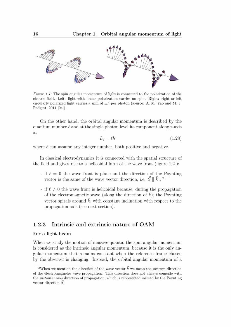
The spin of the photon is connected to the helicity and is described by thecircular polarization basis. The single photon spin along a fixed axis, e.g.z-axis, is:

Sz = sz~ (1.27)

where sz can assume only two values: sz = ±1. All the other values arepossible only in beams of light, as superposition of the spin values of differentphotons. In light beams the spin angular momentum is connected to thepolarization (figure 1.1):

sz = 0 for linearly polarized waves,

sz = +1 for waves with right circular polarization,

sz = −1 for waves with left circular polarization,

−1 < sz < 1 for elliptically polarized waves.

A deeper explanation of the concept of spin can be found in appendix A.


Figure 1.1: The spin angular momentum of light is connected to the polarization of theelectric field. Left: light with linear polarization carries no spin. Right: right or leftcircularly polarized light carries a spin of ±~ per photon (source: A. M. Yao and M. J.Padgett, 2011 [94]).

On the other hand, the orbital angular momentum is described by thequantum number ℓ and at the single photon level its component along z-axisis:

Lz = ℓ~ (1.28)

where ℓ can assume any integer number, both positive and negative.

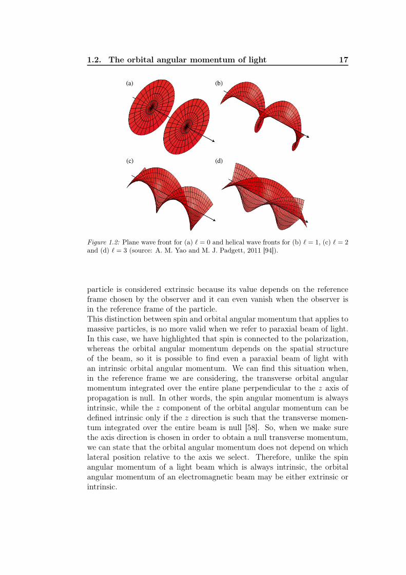
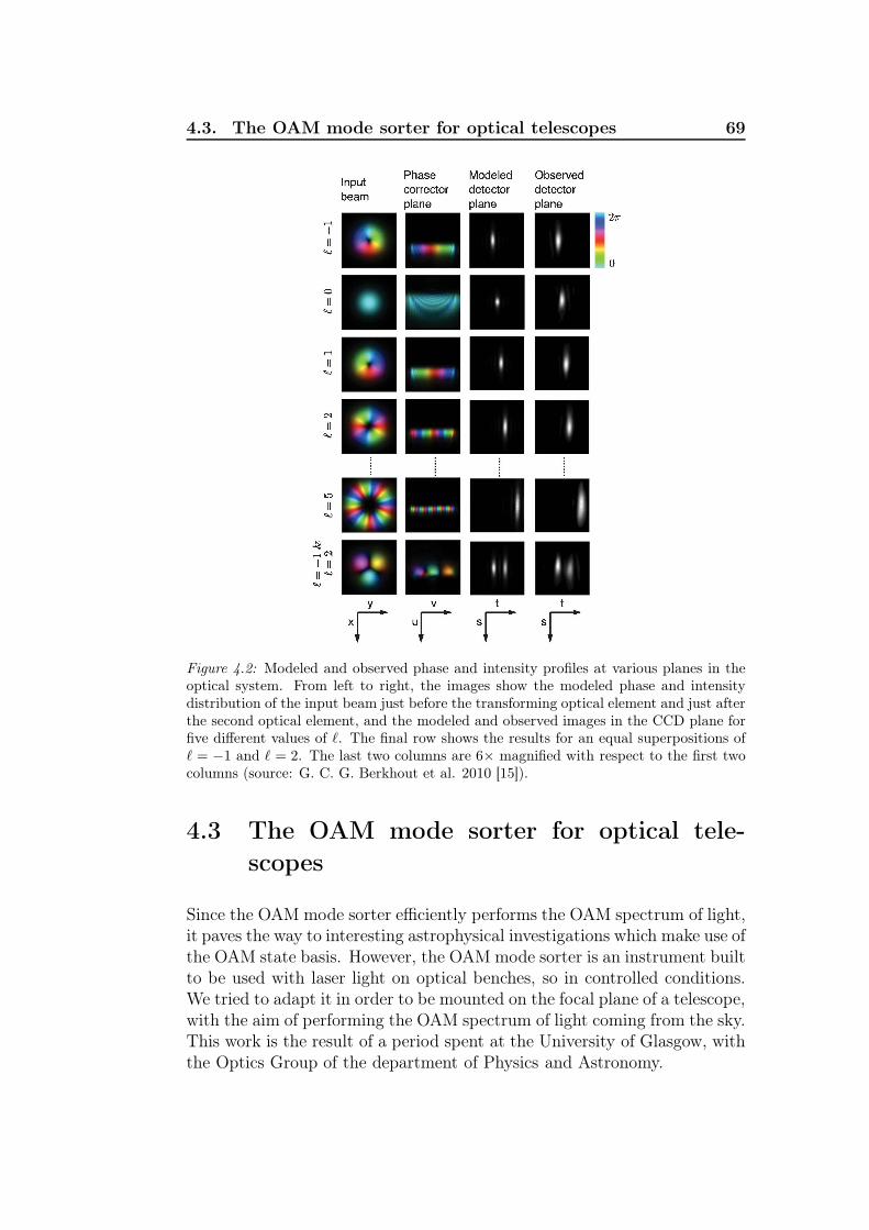
In classical electrodynamics it is connected with the spatial structure ofthe field and gives rise to a helicoidal form of the wave front (figure 1.2 ):

- if ℓ = 0 the wave front is plane and the direction of the Poyntingvector is the same of the wave vector direction, i.e. ~S ‖ ~k ; 2

- if ℓ 6= 0 the wave front is helicoidal because, during the propagationof the electromagnetic wave (along the direction of ~k), the Poyntingvector spirals around ~k, with constant inclination with respect to thepropagation axis (see next section).

1.2.3 Intrinsic and extrinsic nature of OAM

For a light beam

When we study the motion of massive quanta, the spin angular momentumis considered as the intrinsic angular momentum, because it is the only an-gular momentum that remains constant when the reference frame chosenby the observer is changing. Instead, the orbital angular momentum of a

2When we mention the direction of the wave vector ~k we mean the average directionof the electromagnetic wave propagation. This direction does not always coincide withthe instantaneous direction of propagation, which is represented instead by the Poyntingvector direction ~S.


Figure 1.2: Plane wave front for (a) ℓ = 0 and helical wave fronts for (b) ℓ = 1, (c) ℓ = 2and (d) ℓ = 3 (source: A. M. Yao and M. J. Padgett, 2011 [94]).

particle is considered extrinsic because its value depends on the referenceframe chosen by the observer and it can even vanish when the observer isin the reference frame of the particle.This distinction between spin and orbital angular momentum that applies tomassive particles, is no more valid when we refer to paraxial beam of light.In this case, we have highlighted that spin is connected to the polarization,whereas the orbital angular momentum depends on the spatial structureof the beam, so it is possible to find even a paraxial beam of light withan intrinsic orbital angular momentum. We can find this situation when,in the reference frame we are considering, the transverse orbital angularmomentum integrated over the entire plane perpendicular to the z axis ofpropagation is null. In other words, the spin angular momentum is alwaysintrinsic, while the z component of the orbital angular momentum can bedefined intrinsic only if the z direction is such that the transverse momen-tum integrated over the entire beam is null [58]. So, when we make surethe axis direction is chosen in order to obtain a null transverse momentum,we can state that the orbital angular momentum does not depend on whichlateral position relative to the axis we select. Therefore, unlike the spinangular momentum of a light beam which is always intrinsic, the orbitalangular momentum of an electromagnetic beam may be either extrinsic orintrinsic.


For a single photon

If we consider a single photon, its intrinsic properties are:

- null mass,

- null electrical charge,

- spin quantum number equal to 1.

These three properties define a photon, and do not depend on the chosenreference frame.Orbital angular momentum is associated with the phase profile of the lightbeam and directly depends on the spatial coordinates: because of this, itis not an intrinsic property of photons, it is a property of the field. It canbe defined for a single photon [45], but it depends on the reference frameused. Indeed, to define the OAM of a single photon, we need at least twophotons (one used as a spatial reference for the other) or an axis to be usedas a reference frame. So, we can define the OAM of a single photon, butthis measurement requires an appropriate set-up of the experiment.In [83], Tamburini and Vicino discussed that the OAM of a photon is an ex-trinsic property, i.e. OAM of a single photon depends on the used referenceframe.

1.3 Paraxial beams of light: the Laguerre-Gaussian

modes

In quantum mechanics the wave function describing a specific state of theanalyzed system is represented by a vector in a space defined by a completeset of basic and arbitrary functions in a Hilbert space. The square of theabsolute value of the components of such a vector along the axes of theadopted reference frame gives the probability to find our system in the statesidentified by the corresponding eigenvector axes. Analogously, the fieldamplitude of an electromagnetic wave can be described by using differentorthonormal bases.The modern study of optical angular momentum [25] can be said to havestarted with the paper of Allen et al. [2]. In this work it was found thatLaguerre-Gaussian light beams possess an orbital angular momentum ofℓ~ per photon, where ℓ is the so-called azimuthal index of the beam. Thispaper showed that any beam with the following expression for the amplitude

1.3. Paraxial beams of light: the Laguerre-Gaussian modes 19

distribution in cylindrical coordinates3:

u(r, θ, z) = u0(r, z)eiℓθ (1.29)

carried orbital angular momentum about the beam axis4. The orbital con-tribution is determined solely by the azimuthal phase dependence and isequivalent to ℓ~ per photon. A Laguerre-Gaussian beam, familiar fromparaxial optics, is a physically realizable example of light with this phasedistribution.

In the following sections, we are going to analyze light beams emittedby lasers under paraxial conditions (i.e., when the second order aberrationscan be neglected), because under these conditions the separation of opticalangular momentum into spin and orbital parts is straightforward. On theother hand, in exact (or non-paraxial) beams with exp(iℓθ) dependence,neither the spin nor the OAM are physically observable quantities. Indeed,in a general situation, the polarization and spatial degrees of freedom arecoupled by Maxwell equations [9]. However, in beams with sizes muchlarger than the wavelength, which thus propagate in paraxial regime, bothproperties may be controlled separately.

Paraxial beams in a refractive medium

If the beam propagates paraxially in vacuum or in a homogeneous andisotropic medium, Lz and Sz are separately conserved. On the other hand,the anisotropy of a medium acts on the polarization and affects SAM,whereas the inhomogeneity of a medium acts on the wavefront and affectsOAM [18]5.

1.3.1 Paraxial beams and nature of the orbital angular

momentum

It is evident from equation (1.9) that the linear momentum of a plane wavelies along the direction of propagation (which we suppose to be along the zaxis), so there cannot be any component of the angular momentum along

3If we consider a plane perpendicular to the propagation axis z, r is the distance fromthe propagation axis and θ is the azimuthal angle.

4In the literature, the argument of the exponential term can be expressed both with+ and with − sign, it makes no difference for the discussion.

5Whenever SAM and OAM affect each other during propagation, optical spin-orbit

coupling effects take place . A special case of spin-orbit coupling effect is SAM-OAM

conversion, which is defined as an optical process in which SAM and OAM both varyduring propagation but the total angular momentum is conserved, whatever the inputstate of light is [12, 50].


this direction. However, the electric and magnetic fields generated by a laserare not perfectly transverse, but they have some small components alongdirection z. Considering these beams of polarized laser light, the electricfield in cylindrical coordinates (r, θ, z)6 has the following form:

~E(~r, t) = σu(r, θ, z)ei(kz−ωt) + c.c. (1.30)

where σ is the polarization unit vector, ω is the angular frequency of the elec-tromagnetic wave, c.c. represents the complex conjugate, and the complexfunction u(r, θ, z) is a function describing the form of the field amplitudeprofile, and is defined as:

u(r, θ, z) = u0(r, z)eiℓθ. (1.31)

We notice that the total phase of the field has acquired a new component,so now we have:wave phase = kz − ωt + ℓθ .The component ℓθ, where θ is an angle, is the azimuthal phase: it is be-cause of the presence of an azimuthal component of the linear momentumdensity that the orbital angular momentum arises [3]. In fact, in the casewhere the electric field and the magnetic field are transverse to the prop-agation direction ~k, the linear momentum density ~p = ε0

~E × ~B is parallelto ~k and therefore the integration of the angular momentum density (whichvaries according to the position with respect to the considered z axis, butwhich is always perpendicular to ~k) turns out to be equal to zero. So, whenthe electromagnetic wave fields have no components along the propagationdirection ~z, there is no orbital angular momentum. Instead, when the elec-tric field and the magnetic field of the electromagnetic wave have also acomponent along ~k 7, the linear momentum density is no more parallel to~k, therefore the radial and azimuthal components of ~Sp appear. This lastcomponent, in its turn, gives origin to an angular momentum density nomore perpendicular to ~k: in this way, when it is integrated, it does notcompletely cancel out, but a component along ~k remains still present. Ifthose conditions are valid,

~J =1

c2

∫~r × ~Spdτ = ~Jz 6= 0 when Ez 6= 0, Bz 6= 0, (1.32)

then the Poynting vector ~Sp spins around the average propagation direction,and in this way it creates a helicoidal wave front and gives rise to the or-bital angular momentum. It’s important to put in evidence again that it is

6From now on it will be convenient the use of cylindrical coordinates (z, r, θ), withthe z axis coinciding with the average direction of the field’s propagation.

7In this ~kcase represents only the average propagation direction, but not the instan-taneous one, i.e. the direction of the Poynting vector ~Sp is not constant.


fundamental the existence of the electric and the magnetic field componentsalong ~k: thanks to them the azimuthal and radial components of the linearmomentum density are created, and when they are vectorially multipliedwith ~r, they generate a component of the angular momentum density alongz, so that ~J = ~Jz 6= 0We said that (1.31) is the complex scalar function describing the field ampli-tude distribution of a wave carrying OAM, and satisfying the wave equationin paraxial approximation conditions (i.e. | ∂2ψ

∂z2|≪ k | ∂ψ

∂z|). In this

approximation we do not consider the second derivative with respect tothe z coordinate, so there are no second order aberrations. One can easilydemonstrate that under these conditions the radial and azimuthal compo-nents along the z-axis of the linear momentum density ~p = ε0

~E × ~B for acircular polarized beam propagating in the z direction are:

pr = ε0ωkrz

z2R + z2

|u|2, (1.33)

pθ = ε0

[ωℓ

r|u|2 − 1

2ωsz

∂|u|2∂r

], (1.34)

pz = ε0ωk|u|2. (1.35)

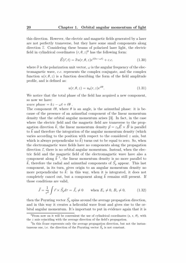
The component (1.33) is due to the divergence of the beam during its prop-agation. The first term of (1.34) depends on ℓ, where ℓ~ has been definedas the orbital angular momentum along z for the single photon; the secondterm is related to the spin, where sz~ is the spin angular momentum alongz of the single photon. The last component, (1.35), is the linear momentumin the propagation direction.

In the description of the field given by Laguerre-Gaussian modes (an-

Figure 1.3: The trajectory of the Poynting vector and the components of linear momen-tum density (source: Allen et al. 1992 [2]).


alyzed in the next section), the temporal average of the real part of thelinear momentum density of arbitrarily polarized light is given by:

ε0

2( ~E∗ × ~B + ~E × ~B∗) = iω

ε0

2(u∗~∇u − u~∇u∗) + ωkε0|u|2z + ωsz

ε0

2

∂|u|2∂r

θ

(1.36)where the first two terms are independent from polarization (one can demon-strate that the gradient is only on the azimuthal phase) and depend on thestructure of the beam phase, while the last term depends on the polariza-tion state and the gradient of the beam intensity [2]. So it is important tonotice that:

- the orbital terms are generated by the phase gradient;

- the spin term is related to the polarization and the intensity gradient.

1.3.2 The Laguerre-Gaussian modes

The field amplitude of a laser light beam is well described by the Laguerre-Gaussian (LG) modes: in the paraxial approximation such modes satisfyMaxwell’s equations [56] and represent the form of the amplitude profilesof the electric field inside a laser cavity 8. Since the electric and mag-netic fields in laser beams are not perfectly transverse, in Laguerre-Gaussianmodes appears the term exp(−iℓθ) which encodes an azimuthal phase and,consequently, an azimuthal angular momentum additional to spin angularmomentum. These modes have a rotational symmetry along their own axisof propagation and an intrinsic orbital angular momentum ℓ~ for the singlephoton.It is useful to express most beams in a complete basis set of orthogonalmodes. For OAM carrying beams this is most usually the Laguerre-Gaussianmode set. Indeed, the analogy between quantum mechanics and optics inparaxial conditions9 suggests that these modes are the autofunctions ofthe orbital angular momentum operator Lz. Thus, the Laguerre-Gaussianmodes define a basis for the orbital angular momentum description in parax-ial light beam, i.e. they constitute a complete set of orthonormal autofunc-tions, which are solutions of the paraxial wave equation.

8One can say the same for the Hermite-Gauss modes.9There is a powerful analogy between paraxial optics and quantum mechanics. Here

the Schrödinger wave equation is identical to the paraxial form of the wave equation witht replaced by z. The analogy allows much of paraxial optics, including orbital angularmomentum, to be studied using the formalism of quantum mechanics.


A Laguerre-Gaussian mode has amplitude:

upl(r, θ, z) =C

(1 + z2/z2R)1/2

[r√

2

w(z)

]ℓLlp

[2r2

w2(z)

]exp

[ −r2

w2(z)

]exp

[ −ikr2z

2(z2 + z2R)

]×

× exp(−iℓθ) exp

[i(2p + ℓ + 1) tan−1

(z

zR

)]

(1.37)

where zR is the Rayleigh range, w(z) is the beam waist, Lℓp is the associated

Laguerre polynomial, and C is the constant of normalization. The integersp and ℓ are indices characterizing the different Laguerre-Gaussian modes:

- the index ℓ represents the number of helices interweaving each otherwithin the space of a wavelength λ and is equal to the OAM parameterℓ; when Laguerre-Guassian modes are interfered with a plane wave,we observe on a screen ℓ spiral arms (fig. 1.4);

Figure 1.4: On the left: wave front shapes for different ℓ values. In the middle: LGintensity patterns on a plane perpendicular to the propagation direction. On the right:intensity patterns on a plane perpendicular to the propagation direction for Laguerre-Gaussian beams interfered with a plane wave. p = 0 for each beam. (source: OpticsGroup of the University of Glasgow, www.physics.gla.ac.uk/Optics/Miles).

- the index p constitutes the number of radial nodes; (p + 1) is thenumber of rings we see on a screen when we observe a Laguerre-Gaussian beam (fig. 1.5).


Figure 1.5: Laguerre-Gaussian intensity patterns, for different ℓ and pvalues (source: Sasada Lab., Department of Physics, Keio University,http://www.phys.keio.ac.jp/guidance/labs/sasada/research/orbangmom-en.html).

When ℓ = 0 and p = 0 Laguerre-Gaussian modes reduce to Gaussian modes(i.e. modes where the function describing the spatial distribution of thefield in the plane perpendicular to the propagation direction is a Gaussianfunction) because the beam has no orbital angular momentum.Instead, for a Laguerre-Gaussian mode with ℓ 6= 0, surfaces of constantphase have helicoidal form and the resulting phase discontinuity (the singu-larity) which is present along the axis, causes the annulment of the intensityalong the axis.

1.3.3 The Poynting vector in Laguerre-Gaussian modes

If we neglect small terms in the z coefficient, the Poynting vector for aLaguerre-Gaussian mode with linear polarization becomes [62]:

~Sp = Czr

z2r + z2

( zr

z2r + z2

r +ℓ

krθ + z

)(1.38)

where z is the distance from the beam waist, zr is the Rayleigh range,k is the wave number, and C is a constant which depends on the radialposition within the intensity distribution, the wavelength of the light and isproportional to the total power in the beam. The presence of the componentθ implicates that the Poynting vector has an azimuthal component duringits propagation: therefore it spirals around the propagation axis, as we cansee in figure 1.6.Let us summarize: the intensity pattern projected by a LG beam on a screenperpendicular to the propagation direction has the following characteristcs:

- if ℓ = 0

- for p = 0: Laguerre-Gaussian modes reduce to Gaussian modes,the beam has no orbital angular momentum. The Poynting vec-tor is parallel to the z axis, giving rise to a spot of light withintensity decreasing from the spot’s center to outside, accordingto a typical gaussian profile;

1.4. Optical vortices 25

Figure 1.6: The helical wavefront characterized by an azimuthal phase term (ℓ = 1) andthe associated Poynting vector, the azimuthal component of which gives rise to an orbitalangular momentum (source: Torres et al. 2011 [88])

- for p 6= 0: a central spot of light is still present, and around itthere are p concentric rings;

- if ℓ 6= 0: the Poynting vector, spinning around the z axis, creates a fielddistribution with (p + 1) maxima, which originate (p + 1) concentricrings around a singularity with null intensity. The radius of the ringsis proportional to the ℓ value.

From equation (1.38) we find that, away from the beam waist, the azimuthalrotational velocity is given by:

∂θ

∂z=

ℓ

krz2. (1.39)

From this equation we see that, fixing constant the radius, the Poyntingvector follows a spiral path, characterized by a constant angle between ~Spand ~k, given by

θ =ℓ

kr(1.40)

and by a step zp necessary to carry out a complete rotation of 360, expressedas:

zp =2πkr2

ℓ. (1.41)

We notice that zp ∝ r2, so in the proximity of the z axis the Poynting vectorspirals around ~k with a short step, whereas moving away from the axis ofthe beam we find that ~Sp spirals with a step greater and greater, infinite tothe limit (see figure 1.7).

1.4 Optical vortices

Traditionally wave propagation is analyzed by means of regular solutions ofwave equation. These solutions often have some singularities, namely some


Figure 1.7: Propagation of the Poyinting vector associated to the different rings of theLaguerre-Gaussiam mode p = 3, ℓ = 1 (source: Allen et al. 1995 [62]).

points or lines in the space where the mathematical quantities describingthe physical properties of waves become infinite or change abruptly. Forexample, a phase singularity is a point where the wave phase is undefinedand intensity vanishes. Phase singularities can be found in every type ofwave, from tidal waves whose singularity is the point at which all cotidallines meet and at which tide height vanishes giving rise to a whirlpool, toelectromagnetic waves.In waves of light, phase singularities [19, 21] form the so-called opticalvortices. Phase singularities are topological features of the wave front,which one can find in light beams having orbital angular momentum: in-deed, the helicoidal form of wave front causes an indetermination of phaseon the axis around which the wave front wraps itself up. This wave frontdiscontinuity along the axis has a null field intensity associated, due to thedestructive interference of all the different wave phases which meet alongthe axis [47]. In other words, the phase of an electromagnetic wave carryinga certain quantity of orbital angular momentum turns out to be undefinedalong the propagation axis, because it is where different wave phases join,giving rise to destructive interference. Therefore such phase singularitiesof the wave function appear as points where the wave function modulusbecomes equal to zero, and are called dislocations or optical vortices: sucha name is due to the structure of the surface of constant phase, which lookslike a dislocation with the form of a helix, and to the direction of the phasegradient, which spins and wraps itself up around the singularity line, simi-larly to a fluid in a water whirlpool. The Poynting vector spins around thevortex nucleus in a given direction: from equation (1.39) we infer that atthe centre of the vortex this rotational velocity is infinite. So, the featuresof an optical vortex are essentially two (fig. 1.8):


1. a wave front with a helicoidal form, therefore the beam of light isendowed with orbital angular momentum,

2. a wave front discontinuity along the propagation direction, thereforea phase discontinuity: light intensity is equal to zero along that axis(no more gaussian spot of light, but rings of light around a singularitywith null intensity).

Figure 1.8: The wave front (top) and the intensity pattern (bottom) of the simplestLaguerre-Gaussian mode. The index ℓ is referred to as the winding number, and (p + 1)is the number of radial nodes. Here we only consider the case of p = 0. The azimuthalphase term exp(iℓθ) of the Laguerre-Gaussian modes results in helical wave fronts. Thephase variation along a closed path C around the beam center is 2πℓ. Therefore, in orderto fulfill the wave equation, the intensity has to vanish in the center of the beam (source:Mair et al. 2001 [47]).

Phase singularities (or dislocations, or optical vortices) are characterizedby the fact that phase undergoes a changing of an entire multiple of 2πalong a closed circuit C around the middle of the vortex (fig. 1.9). As aconsequence, it becomes useful to define the concept of topological charge ofan optical vortex. We remind that, in order to describe the field amplitude,we have defined a complex scalar function given by eq. (1.31), which canbe expressed also in the following way:

u(~r) = |u(~r)|eiχ(~r) (1.42)

where χ(~r) represents the phase of the wave amplitude.


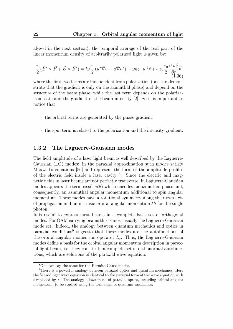
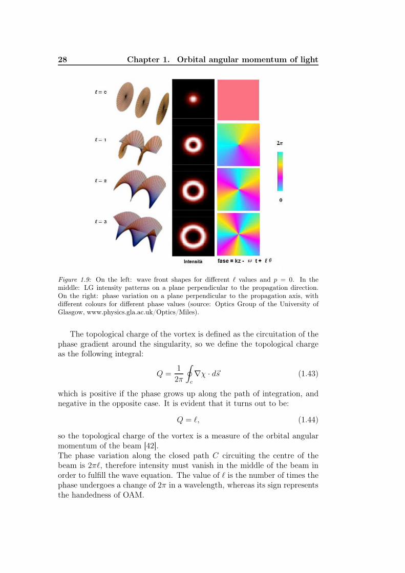
Figure 1.9: On the left: wave front shapes for different ℓ values and p = 0. In themiddle: LG intensity patterns on a plane perpendicular to the propagation direction.On the right: phase variation on a plane perpendicular to the propagation axis, withdifferent colours for different phase values (source: Optics Group of the University ofGlasgow, www.physics.gla.ac.uk/Optics/Miles).

The topological charge of the vortex is defined as the circuitation of thephase gradient around the singularity, so we define the topological chargeas the following integral:

Q =1

2π

∮

c

∇χ · d~s (1.43)

which is positive if the phase grows up along the path of integration, andnegative in the opposite case. It is evident that it turns out to be:

Q = ℓ, (1.44)

so the topological charge of the vortex is a measure of the orbital angularmomentum of the beam [42].The phase variation along the closed path C circuiting the centre of thebeam is 2πℓ, therefore intensity must vanish in the middle of the beam inorder to fulfill the wave equation. The value of ℓ is the number of times thephase undergoes a change of 2π in a wavelength, whereas its sign representsthe handedness of OAM.


Optical vortices in Nature

Optical vortices do not represent a purely artificial feature of light (orig-inated, for example, when a beam of laser light goes through a hologramcreated by computers, or a spiral phase plate [11, 89]), but can be generatednaturally by some deformations of the wave front, which can be caused bythe passing through a non linear medium.Anisotropic optical vortices occur in speckle patterns, which arise naturallyfrom the interference of a large number of more or less random plane waves[17]. At particular places in a speckle pattern the amplitude of the field van-ishes, causing the phase to be singular. Around these phase singularitiesan optical vortex is formed, whose exact form is determined by the localinterference of plane waves. Natural optical vortices are anisotropic, i.e.they still have a complex amplitude with an azimuthal behaviour charac-terized by the term exp(iℓθ) but, unlike isotropic optical vortices, the phaseincrease does not go linear with the azimuth coordinate θ. Not only doesthe phase increase in a nonlinear way around an anisotropic vortex, also theintensity profile around it is anisotropic, i.e. the lines of constant intensityare ellipses (fig. 1.10).Describing the azimuthal behaviour of the field around an anisotropic op-

Figure 1.10: Phase of the field for (a) an isotropic ℓ = 1 optical vortex and (b) ananisotropic ℓ = 1 optical vortex. Black lines (there are eight lines, from the centeroutwards) indicate equal-phase lines and are spaced π/4 radians apart. In (b) the linesare more closely spaced around the y axis, showing the anisotropic character of the vortex.In addition, the dashed lines indicate lines of constant intensity. For an isotropic opticalvortex, the lines of constant intensity are circles, while for an anisotropic optical vortexthey are ellipses (source: Berkhout 2011 [17]).

tical vortex requires more than one pure optical vortex mode, such that thefield can be decomposed in the orthogonal basis of pure vortex modes:

u(θ) =∑

ℓ

cℓ√2π

eiℓθ (1.45)


where the factor 1/√

2π ensures the normalization. The coefficient c0 isrelated to the local intensity of the field, the coefficients c−1 and c+1 arerelated to the derivatives of the field. In the case of an isotropic opticalvortex cℓ = δℓ,m, where δi,j is the Kronecker delta.

The optical vortex coronograph

Light coming from astronomical sources can be manipulated at the tele-scope. We have seen that when a beam of light carries orbital angularmomentum, its intensity vanishes on the propagation axis: this propertyof optical vortices can be used in astronomical field to detect extrasolarplanets. Using appropriate manipulation of light, one can induce orbitalangular momentum in the light coming from the on-axis star, in order toobscure it and allow to observe nearby planets, which otherwise would beinvisible because of the great difference of their magnitude with respectto the star. In this case star light behaves like a coronograph for itself[8, 24, 40, 41, 46, 49, 82].

Chapter 2Photon orbital angular momentum

and mass in a plasma vortex

As astronomers, we are interested in how the orbital angular momentum oflight can be exploited in the field of astronomy:

• astronomers may produce OAM:

- with the so-called optical vortex coronograph, an optical instru-ment that exploits the geometrical properties of optical vorticesto allow seeing very faint objects near very bright objects, thatwould normally be obscured by glare (e.g. extrasolar planets neartheir host star). Vortices are artificially produced by optical el-ements (spiral phase plates) inserted in the optical path of lightthrough the telescope, so that the light of the on-axis source (e.g.the hosting star) is rejected without altering the light of off-axissources (e.g. extrasolar planets) [8, 24, 40, 41, 46, 49, 82];

- to overcome the Rayleigh criterion limit with optical vortices, inorder to resolve two sources at angular distances much below theRayleigh limit [77];

• astronomers may use OAM as a new diagnostic observable of light,in order to get additional information about the Universe [23, 31], inparticular about:

- very massive and rotating objects, e.g. Kerr black holes, sincetheir space-time dragging can imprint OAM on light passingthrough their surroundings [81];

- inhomogeneous plasmas traversed by photons during their travelfrom the astrophysical source to the observer (this is the topicdealt with in this chapter) [80].

31

32 Chapter 2. Photon OAM and mass in a plasma vortex

In this chapter we analyze the mechanism of photon mass acquisition ina plasma and study the contribution to the mass from the orbital angularmomentum acquired by a beam of photons when it crosses a spatially struc-tured charge distribution. To this end we apply Proca-Maxwell equationsin a static plasma with a particular spatial distribution of free charges, no-tably a plasma vortex, that is able to impose OAM onto light. In additionto the mass acquisition of the conventional Anderson-Higgs mechanism, wefind that the photon acquires an additional mass from the OAM and thatthis mass reduces the Proca photon mass.The results exposed in this chapter can be found in the publication "Photonorbital angular momentum and mass in a plasma vortex" [80].

2.1 Introduction

Influenced by results derived in 1962 by Schwinger [71], in 1963 Andersonshowed that a photon propagating in a plasma acquires a mass, called alsoeffective mass, defined as:

meff =~ωpc2

(2.1)

where ωp is the plasma frequency1, ~ is the reduced Planck constant andc is the velocity of light in vacuum [5, 54]. In this process the photon ac-quires an effective mass because of its interaction with plasmons (collectiveoscillations of the free electron gas density at precise frequencies) [53].In order to study photons that have acquired an effective mass, it is con-venient to replace Maxwell’s equations by Proca-Maxwell equations, whichare the equations describing a massive electromagnetic field [29, 37]. In thischapter we are going to use this approach to analyze the contribution to themass from the orbital angular momentum acquired by a beam of photonsas it traverses a spatially structured charge distribution.OAM can be generated by the imprinting of vorticity onto the phase distri-bution of a beam when it crosses inhomogeneous non-linear optical systems[6] or particular spatial structures such as fork holograms or spiral phaseplates. Such a beam can be described by a superposition of Laguerre-Gaussian (LG) modes characterized by the two integer-valued indices ℓ andp [2]. The azimuthal index ℓ describes the number of twists of the helicalwavefront in a wavelength and the radial index p gives the number of radialnodes of the mode. The electromagnetic field amplitude of a generic LG

1Free electrons and positive ions within a plasma have densities oscillating at a naturalfrequency ωp, the plasma frequency. It defines a cutoff frequency below which there isno electromagnetic propagation and the penetrating wave drops off exponentially, whileat frequencies above ωp absorption is small and the plasma is transparent.

2.2. Photons in a static plasma vortex 33

mode, in a plane perpendicular to the direction of propagation, is

Fpl(r, θ) =

√(ℓ + p)!

4πp!

(r2

w2

)|ℓ|

L|ℓ|p

(r2

w2

)e−

r2

2w2 eiℓθ (2.2)

obeying to the orthogonality condition

∫ ∞

0

rdr

∫ 2π

0

F ∗pℓFp′ℓ′dθ = δpp′δ

ℓℓ′ (2.3)

where w is the beam waist, L|ℓ|p is the associated Laguerre polynomial, and

r and θ are the cylindrical coordinates in the plane perpendicular to thedirection of propagation z. As we stated in chapter 1, the phase factorexp(−iℓθ) is associated with an OAM of ℓ~ per photon, and a phase sin-gularity is embedded in the wavefront, along the propagation axis, with atopological charge ℓ [2, 93].As is well known, not only the linear momentum of light but also its angularmomentum can propagate to infinity [38, 72, 85]. The OAM property ofthe field remains stable during the propagation in free space and has beenexperimentally verified down to single-photon limit [58]. It has also beenstudied theoretically [83].Different is the case of photons propagating in inhomogeneous media [39].The exchange of angular momentum between a photon beam and a plasmavortex and the possible excitation of photon angular momentum states ina plasma was analyzed in ref. [55]. In this chapter we show that the OAMacquired by a photon in a spatially structured plasma can be interpreted asan additional mass-like term that appears in Proca equations. More specif-ically, we study the propagation of a photon with wavelength λ in a statichelicoidally distributed plasma with step q0 = λ/b, where b is an integer.The possibility of studying space plasma vorticity remotely by measuringthe OAM of radio beams interacting with the vortical plasma was pointedout by Thidé in 2007 [84]. Here we analyze this possibility theoreticallyby studying the exchange of angular momentum between a plasma mediumand a photon beam.

2.2 Photons in a static plasma vortex

Let us consider an isotropic plasma, cast to form a helicoidal static plasmavortex. The heavy ions constitute a neutralising background and their mo-tion can, in the first approximation, be neglected. If we consider transverseelectromagnetic waves propagating through this kind of plasma, we can


describe them by the electric field propagation equation2

(∇2 − 1

v2ph

∂2

∂t2

)~E = µ

∂~j

∂t(2.4)

where vph = (εµ)−1/2 is the phase velocity of light in a medium with permit-tivity ε and permeability µ, and the electron current~j = −en~v is determinedby the electron fluid equations

∂n

∂t+ ∇ · n~v = 0, (2.5)

∂~v

∂t+ ~v · ∇~v = − e

m( ~E + ~v × ~B). (2.6)

where n is the electron number density, ~v is the velocity of the electrons inthe medium, e is the electron electric charge and m is the electron mass.Thermal and relativistic mass effects are ignored.The presence of a static plasma perturbation with helical structure bringsabout a new definition of the mean electron velocity and density, whichbecome:

~v = ~v0(~r, t) + δ~v (2.7)

where ~v0 is the background velocity and δ~v is the perturbation associatedwith the propagating electromagnetic wave, and

n = n0 + n(r, z) cos(ℓ0θ + q0z) (2.8)

where n0 is the background plasma density, and the plasma helix vortexdensity perturbation is described by the second term. It is expressed incylindrical coordinates, ~r ≡ (r, θ, z), and it depends on the distance withrespect to the vortex axis of symmetry and can vary slowly along z, on ascale much longer than the spatial period z0 = 2π/q0 (where q0 is the helixstep)3 .So, ignoring the plasma rotation and considering the case of a static helicalperturbation, the current density of the plasma now becomes ~j = −en(~r)δ~v,and the propagation equation of the electric field takes the following form:

∇2 − 1

v2ph

∂2

∂t2−

ω2p0

v2ph

[1 + ε(r, θ, z)]

~E = 0 (2.9)

where

ω2p0 =

e2n0

ε0m(2.10)

2We use MKS system of units.3For a typical double vortex we will have ℓ0 = 1.


represents the square of the frequency of the plasma with no density per-turbation (where ε0 is the permittivity of free space), and

ε(r, θ, z) =n(r, z)

n0cos(ℓ0θ + q0z) (2.11)

expresses the vortex perturbation.We further assume that waves propagate along the vortex axis Oz, andconsider solutions of the form

~E(~r, t) = ~A(~r) exp

[−iωt + i

∫ z

k(z′)dz′]

(2.12)

where ω is the wave frequency, k = 2π/λ is the wave number, and ~A(~r) isthe wave amplitude: it varies slowly along z and satisfies 4

∣∣∣∣∣∂2 ~A

∂z2

∣∣∣∣∣ <<

∣∣∣∣∣2k∂ ~A

∂z

∣∣∣∣∣ . (2.13)

We can reduce the wave equation (2.9) to the perturbed paraxial equation:[

∇2⊥ + 2ik

∂

∂z−

ω2p0

v2ph

ε(r, θ, z)

]~A = 0 (2.14)

with the dispersion relation connecting k and ω that has the form:

k2 =1

v2ph

(ω2 − ω2p0). (2.15)

We observe that if there was no vortex perturbation, equation (2.14) wouldreduce to the usual paraxial optical equation 5. Instead, considering ourcase characterized by a vortex perturbation, a general solution to the waveequation in the paraxial approximation can be represented in a basis oforthogonal Laguerre-Gaussian modes, according to the expansion [55]

~A(r, θ, z) =∑

pℓ

Apℓ(r, z)eiℓθe−r2

2w2 epℓ (2.16)

where w ≡ w(z) is the beam waist, epℓ are unit polarization vectors and Apℓ

are the amplitudes, defined by

Apℓ(r, z) = Apℓ(z)

√(ℓ + p)!

4πp!

(r2

w2

)|ℓ|

L|ℓ|p

(r2

w2

)(2.17)

4Equation (2.13) states that an acceleration (the term on the left) is much smaller thanthe corresponding velocity (the term on the right), and so it mathematically expresses

that ~A(~r) varies slowly along z.5The paraxial equation is the equation describing the wave in the immediate vicinity

of the optical axis.


where L|ℓ|p (x) are the associated Laguerre polynomials, the integer p is the

radial quantum number and ℓ is the azimuthal quantum number. Substi-tuting equation (2.16) in equation (2.12), we can express the total electricfield as a superposition of Laguerre-Gaussian states:

~E(~r, t) =∑

pℓ

~Epℓ(~r) exp

(−iωt + i

∫ z

k(z′)dz′)

(2.18)

with~Epℓ(~r) = ~Apℓ(z)Fpℓ(r, θ) (2.19)

where Fpℓ(r, θ) is the one given in eq. (2.2). When a vortex perturbationε(r, θ, z) is present, these modes will be coupled to each other through therelation [55]

∂

∂zApℓ(z) =

i

2kv2ph

∑

p′ℓ′

K(pℓ, p′ℓ′)Ap′ℓ′ (2.20)

where K(pℓ, p′ℓ′) are the coupling coefficients, defined by:

K(pℓ, p′ℓ′) = ω2p0

∫ ∞

0

rdr

∫ 2π

0

F ∗pℓFp′ℓ′ε(r, θ)dθ. (2.21)

They can be reduced to

K(pℓ, p′ℓ′) = ω2p0δpp′

∫ 2π

0

ε(θ)ei(ℓ′−ℓ)θdθ (2.22)

when we consider the simplest case, that is the case when ε depends onlyon the azimuthal angle θ 6.Let’s try to understand the physical meaning of the mode coupling. Wehave to imagine that the photon, traveling through the static plasma vor-tex, bumps into the electrons forming the vortex, and the different andsubsequent impacts generate the photon orbital angular momentum. Ob-viously, there is not a transfer of a sharp OAM characterized by a precisetopological charge l, but as long as the photon goes through the plasma, ithits electrons and, by this way, acquires orbital angular momentum.

Generally speaking, it is important to highlight that the superposition ofstates is different from the coupling. In fact, in superposition the differentstates are independent, while in coupling the different states depend oneach other, according to a defined relation. So, in coupling, a mode is notnecessarily composed by all the other modes. An example is given by thecase analyzed right now: the mode coupling is weak, and so it is simplygiven by a basic mode and some perturbations.

6This expression remains valid when the radial scale of the plasma vortex is muchlarger than the photon beam waist w(z).


Special solution: photon beam with no initial OAM

Now we want to analyze the special case of:

- a photon beam with no initial OAM, and that can be described by~Epl = 0 for l 6= 0. We are particularly interested in this case becauseordinary stars should not emit OAM, so starlight traversing interstel-lar plasma should have no initial orbital angular momentum;

- a mode coupling sufficiently weak to consider the zero OAM modedominant over the entire interaction region, such that |Ep0| >> |Ep′l′ 6=0|.We are interested in this assumption because it reflects the character-istics of rarefied astrophysical plasmas.

So, starting from a helical static plasma perturbation defined by equation(2.9), with these assumptions we obtain [55]:

K(pl, p′l′) = πω2p0

n

n0

δpp′[δl′,−l0eiq0z + δl′,l0e

−iq0z] (2.23)

Now we substitute this expression of the coupling coefficients in the coupledmode equation (2.20), then we integrate over the axial coordinate z andfinally we obtain Apl(0) = A(0)δl0. If we assume the same polarizationstate for all the interacting modes, we find that the field mode amplitudesare given by

Ap,±l0(z) = iπA(0)

2c2

∫ z

0

ω2p0(z

′)

k(z′)

n(z′)

n0e∓iq0z

′

dz′. (2.24)

The rate of transfer of OAM from the static plasma vortex to the electro-magnetic field is described by this equation. We have to notice that thislast equation is only valid when the transfer of OAM is small, such thatthe amplitude of the initial Gaussian mode Ap0 can be considered constantalong the axis.

General solution: photon beam with an initial OAM

A more general solution, where the amplitude of the initially excited modeis allowed to change, is discussed in ref. [55]. The authors show that theinitial OAM state ℓi of the electromagnetic beam passing through the vortexplasma decays over all the other states (ℓi + uℓ0), where u is an integer,on a length scale approximately determined by the inverse of the couplingconstant, showing an effective exchange of OAM states between photonsand plasma.


2.3 Proca equations

When one considers a photon propagating in a plasma, the usual Maxwell’sequations can be replaced by the set of Proca equations (or Maxwell-Procaequatios) in which there appears a mass-like term for the photon due tolight-matter interaction [37].In the presence of charges ρ and currents

−→j , the three-dimensional version of

the Proca equations, can be written in terms of the electric ~E and magnetic~B fields (in SI units) as:

∇ · −→E =ρ

ε0

− µ2γφ (2.25)

∇×−→E = −∂

−→B

∂t(2.26)

∇ · −→B = 0 (2.27)

∇×−→B = µ0j + µ0ε0

∂−→E

∂t− µ2

γ

−→A (2.28)

(where ε0 and µ0 are the permittivity and the permeability of free spacerespectively) together with the equations

~B = ∇× ~A (2.29)

~E = −∂ ~A

∂t−∇φ (2.30)

and the Lorentz condition

∇ · −→A = − 1

c2

∂φ

∂t(2.31)

where−→A is the vector potential, c = (ε0µ0)

−1/2 is the phase velocity oflight in vacuum, and φ is the scalar potential. µ−1

γ is a characteristic lengthassociated with the photon rest mass mγ by the relation:

mγ =µγ~

c(2.32)

For mγ tending to zero, Proca equations smoothly reduce to Maxwell’sequations.The Poynting vector for massive photons depends directly on both the scalarand the vector potentials

−→S =

1

µ0

(−→E ×−→

B + µ2γφ

−→A ) (2.33)

and also the energy density of the massive electromagnetic field has anexplicit dependency on the potentials

u =1

2(ε0

−→E 2 +

1

µ0

−→B 2 + ε0µ

2γφ

2 +1

µ0µ2γ

−→A 2). (2.34)

2.3. Proca equations 39

2.3.1 Proca equations for photons in a plasma

We have seen that a photon in a plasma gains an effective mass. On theother hand we have seen Proca equations, which are equations describingmassive photons. Therefore we can try to use Proca equations to describethe motion of photons in a plasma.Before starting our analysis, it is important to remark that the scalar poten-tial φ appearing in Proca equations and in the expression of the Poyntingvector and of the energy density u for a massive electromagnetic field mustbe set equal to zero. In fact we know that along a fixed direction, e.g.the z direction, the photon has spin with only two values, ±1, the thirdcomponent Sz = 0 does not have meaning because it is not a property ofthe photon. So the photon rest mass has to be null because, according toHeitler, if the photon had a finite rest mass, three independent polarizationswould exist, including a longitudinal polarization [35]. In a plasma thereis not an effective longitudinal component of polarization, because the onewe find actually is given simply by the scattering processes with electrons,and not by a a real intrinsic nature of the photon. Therefore the lack ofthis third spin component induces to consider equal to zero the photon restmass. As a consequence φ must be null, because such a scalar field is alsomassive.

If we want to apply Proca equations to the plasma case, we have to insertthe effective photon mass that a photon acquires going through a plasma.The photon mass in Proca equations is expressed by equation

mγ =µγ~

c(2.35)

whereas the effective photon mass is

meff =ωp~

c(2.36)

so, comparing these two equations, the inverse of the characteristic lengthin a plasma, µγ, is equal to the plasma frequency: µγ = ωp.With these assumptions (φ = 0 and µγ = ωp) the equations describing amassive electromagnetic field become:

∇ · −→E =ρ

ε0(2.37)

∇×−→E = −∂

−→B

∂t(2.38)

∇ · −→B = 0 (2.39)


∇×−→B = µ0J + µ0ε0

∂−→E

∂t− ω2

p

−→A, (2.40)

the Poynting vector takes the form

−→S =

1

µ0

(−→E ×−→

B ) (2.41)

and the energy density is expressed by:

u =1

2

(ε0−→E 2 +

1

µ0

−→B 2 +

1

µ0ω2p

−→A 2

). (2.42)

Let’s start to develop the four-dimensional expression of Proca equations inthe case of a plasma. When considering the electromagnetic wave equationof the Proca field, one obtains a Klein-Gordon equation for the 4-vectorpotential Aµ:

( − µ2γ)Aµ = −µ0jµ (2.43)

where = ( ∂2

∂t2−∇2) is the D’Alembertian differential operator. By differ-

entiating this expression with respect to time, and considering the simplestcase where µγ is a constant in time, one obtains

( − µ2γ)

∂

∂tAµ = −µ0

∂

∂tjµ (2.44)

This last equation is constituted by four components, and separating thetemporal component from the spatial one we have:

( − µ2γ)

∂∂t

A0 = µ0∂∂t

ρ

( − µ2γ)

∂∂t

Ai = µ0∂∂t

ji.(2.45)

From now on we are interested only in the second equation of (2.45). Wewant to apply these equations to the case of photons moving in a plasma,in particular we consider the case of a plasma with a well-defined structure,a static plasma vortex. In this case the current density has the form~j = −en(~r)δ~v, so its derivative becomes

∂

∂tji = −e[δ~v

∂

∂tn(~r) + n(~r)

∂

∂tδ~v] = −en(~r)

∂

∂tδ~v (2.46)

where the first term in the square brackets has been eliminated becausewe are considering a static plasma vortex, so the density n = n(~r) is nota function of time. Since we are considering the case of a rarefied plasma(because it is the case of interstellar plasmas), vph ∼ c and from now onwe use the unitary value for the phase velocity of light in vacuum, i.e.

2.3. Proca equations 41

vph ∼ c = 1. Thus, from the second equation in (2.45) and from equation(2.46), in the case of a static plasma vortex one finds

( − µ2γ)

∂

∂t~A = −en(~r)

∂

∂tδ~v. (2.47)

Using equation (2.30) ( ~E = −∇φ − ∂ ~A/∂t) and remembering that we areconsidering a scalar potential φ equal to zero, we can substitute the vectorpotential so that the last equation can be expressed as

( − µ2γ)

~E = en(~r)∂

∂tδ~v. (2.48)

Explicating the D’Alembertian, assuming that δ~v is parallel to ~E (remem-ber that δ~v is the perturbation of electrons velocity associated with thepropagating electromagnetic wave), and substituting from now on the lightvelocity in vacuum (which, in our case, is a good approximation of the phasevelocity of light in the plasma, vph) with the unitary value, c = 1, we canwrite (

∂2

∂t2−∇2 − µ2

γ −en(~r)∂t~v

ε0| ~E|

)~E = 0. (2.49)

We want to compare this last equation (which is an expression of the Procaequations applied to a rarefied plasma, so that vph ∼ c, with a static vortexdensity) to the equation derived by the electric field propagation equationdeveloped for the case of a static plasma vortex, which was:

∇2 − ∂2

∂t2− ω2

p0[1 + ε(r, ϕ, z)]

~E = 0. (2.50)

In order to make equal these last two equations, (2.49) and (2.50), we arriveat the following relation:

µ2γ +

en(~r)

ε0| ~E|= ω2

p0[1 + ε(r, ϕ, z)] (2.51)

where, as we stated previously, ε0 is the permittivity constant of the vacuum,while ε expresses the vortex perturbation. Explicating the ωp0 and ε terms(defined by equations (2.10),(2.11)) we obtain

µ2γ =

e2n0

ε0m+

e2

ε0mn cos(l0ϕ + q0z) − en(r)

ε0| ~E|(2.52)

which after some passages can be written as:

µ2γ =

e

ε0

(e

m− 1

| ~E|

)[n0 − n cos(l0ϕ + q0z)]. (2.53)


This is the key equation, which shows that there is a relation between theeffective mass that a photon acquires in a plasma and the orbital angularmomentum. In fact, if we remember that:

- µγ is related to the photon effective mass gained in a plasma,

- n(r, z) cos(l0ϕ + q0z) is related to the vortex perturbation, which insection (2.2) we showed to cause a transfer of OAM to the electro-magnetic field traversing it

we understand the meaning of equation (2.53):

1- the negative term in the effective photon mass acquired in a turbulentplasma can be interpreted as an expression of orbital angular mo-mentum. It can be considered as a fictitious term, because it is aninteraction term generated by the scattering of photons with electronsin a plasma, and cannot be ascribed as an intrinsic property of thephoton;

2- when the electron number density exhibits certain spatial properties,such as vortices, any photon has an associated virtual mass term thatis smaller than that expected from Proca equations in a homogeneousplasma, because of a negative term that corresponds to a precise or-bital angular momentum component.

So every time a photon goes through a plasma, it gains this virtual massterm that corresponds to a precise orbital angular momentum component, ifthe density of electrons has certain spatial properties. The electron numberdensity does not necessary need to exhibit a vortex structure, what is nec-essary is that it is azimuthally inhomogeneous in the plane perpendicularto the propagation’s direction of the electromagnetic beam.

From an ideal to the real case of OAM transfer

If we want to study the orbital angular momentum gained by a photonpassing through a real plasma, we have to consider the special case of astatic plasma vortex, even if we will never find a plasma with such a precisewell-defined spatial distribution. We are interested in understanding thisparticular case, because it can be used as a basis to build any other type ofstructure. The real problem is extremely complex and difficult to resolve,so we can analyze the simplest special solution, and consider our problemas a superposition of many simple solutions, whose combinations could giveevery possible value of orbital angular momentum.

2.4. Conclusions 43

For example, a simple planar slab of astrophysical plasma with uniform elec-tron spatial density can be represented by the superposition of left-handedand right-handed plasma vortices that gives a final null OAM componentas expected.

2.4 Conclusions

In this chapter we have investigated the problem of photon mass in aninhomogeneous plasma and showed that part of the acquired mass term isrelated to the orbital angular momentum of light imposed by certain spatialdistributions of plasma electrons. We have focused our attention on the sim-plest case of spatial distribution described by a static plasma vortex. Thisapproach shows that the spatial distribution of charges can impose OAM,and that this OAM is related to an additional mass term that reduces theeffective mass of the photon inside a non-structured plasma. When the den-sity function of the traversed plasma is azimuthally inhomogeneous in theplane perpendicular to the propagation’s direction of the electromagneticbeam, we have found that the virtual photon mass term is smaller thanthat expected from Proca equations in a homogeneous plasma, because ofa negative term that corresponds to a precise orbital angular momentumcomponent. In this case, a cascading process of OAM transfer between theplasma and the photon beam is achieved, which is related to the electronnumber density function.Therefore, studying the OAM of light we collect with our telescopes couldgive additional information about the spatial structure of the interstellarmedium traversed by photons during their travel from the source to theobserver. OAM of light could acquire the same importance as spectroscopy:spectroscopy can give us information about the energy of light, while theorbital angular momentum could provide us information about the spatialstructure of the traversed media.


Chapter 3Experimental verification of vorticity

preservation in the far field

In the previous chapter we have shown that the orbital angular momen-tum encoded in a beam of light can bring further information about theuniverse, in particular about the spatial structure of the traversed media[80]. We also know that orbital angular momentum can be imparted by thespace-time dragging of massive rotating sources, so it can bring informationabout these kind of objects, in particular Kerr black holes [81].Therefore, if orbital angular momentum can be seen as an additional carrierof information, now it is important to test if its topology (which is connectedto the orbital angular momentum value) is preserved in the far field. Thischapter deals with an outdoor test we performed, which for astronomicalpurposes has the meaning of an experimental confirmation of a theoreticalprediction, first made almost a century ago by Abraham [1], that the to-tal electromagnetic angular momentum can propagate over huge distances.This test was done in the radio domain: since OAM is a property of theelectromagnetic field, it has the same behaviour at all wavelengths.We have shown experimentally how to propagate and use the properties oftwisted non-monochromatic incoherent radio waves to simultaneously trans-mit two radio channels on the same frequency encoded with different orbitalangular momentum states. The positive outcome of this experiment showsthat:

- non-monochromatic incoherent waves (which are interesting in thefield of astronomy, since they are the main kind of light astronomerscollect with their instruments) preserve their orbital angular momen-tum signature in far field;

- OAM states are orthogonal states, they do not influence each other,and their orthogonality is preserved.

45

46 Chapter 3. Verification of vorticity preservation in far field

Apart from the field of astronomy, in the radio domain the natural con-sequence of these properties is a novel radio technique, which allows theimplementation of, in principle, an infinite number of channels in a given,fixed bandwidth, even without using polarization, multiport or dense cod-ing techniques.The results exposed in this chapter can be found in the publication "En-coding many channels on the same frequency through radio vorticity: firstexperimental test" [78].

3.1 Introduction

Here we report the results of real-world, outdoor radio experiments in the2.4 GHz band (it’s the same band than WiFi). The results reported hereshow that OAM and vorticity are preserved throughout the long-distancepropagation. Therefore, from an astronomical point of view, i.e. when weare the receivers of electromagnetic radiation, this means that the messagebrought by light can arrive to us 1; from a telecommunications point of view,when we are also the transmitters, this means that OAM states can be usedas a new and very large set of communication channels that are mutuallyorthogonal to each other in the OAM state space [86].Our findings extend previous indoor laboratory test experiments in whichthe transmission of optical OAM states [28] and radio [79] beams wasdemonstrated.

3.2 Our apparatus: technical details

In our radio vorticity communication experiments, we generated and de-tected two orthogonal OAM channels within a fixed frequency band: oneuntwisted with OAM ℓ = 0 and the other with an ℓ = 1 OAM twist. Twoidentical WiFi FM transmitters, each with an output power of 2 Watt anddriven by a signal generator, were tuned to the carrier frequency of 2.414GHz to feed two antennae. In an FM transmission the amplitude and inten-sity of the electromagnetic wave remain constant in time, only the carrierfrequency is modulated. The signal-to-noise ratio of the WiFi modules was39 dB for the video channel and 45 dB for the audio band. The receiversensitivity was −90 dBm 2 , i.e. 10−9 mW. The transmitted signal band-widths of both signals were 15 or 27 MHz (like those used in video signals).

1Obviously, for frequency domains affected by the terrestrial atmosphere, this is truewhen we can neglect or compensate for or remove the effects of the turbulent atmosphereon the wave phase.

2The decibel (dB) is a logarithmic unit that indicates the ratio of a physical quantity(usually power or intensity) relative to a specified or implied reference level. A ratio in

3.2. Our apparatus: technical details 47

The ℓ = 0 source was radiated with linear polarization by a commercial 16.5dBi gain Yagi-Uda antenna.To generate the ℓ = 1 vortex beam, we mechanically modified a pair of 26dBi commercial off-axis steel parabolic antennas 3, with 15 offset and di-ameter D = 80 cm, to attain an off-axis spiral parabolic-shaped phase maskreflector. To get the parabolic shape the dish was transformed into a vortexreflector by attacching together the two antennas, one upon the other, andelevating, from the original shape, the surface of the antenna laying on thetop (see fig. 3.1). The elevation, H , depends on the desired ℓ value, and isrelated to the wavelength λ by the following relation:

ℓ =∆n · H

λ(3.2)

where ∆n is the difference between the refractive index of the medium be-fore the wave impinges on the antenna, and the one after. Since in our casewe have a reflection, ∆n = 2. Thus, if our wavelength is λ ∼ 12.5 cm, andif we want ℓ = 1, H has to be ∼ 6.25 cm.The expected beam waist, given by the diffraction limit of the antenna,

is ∆ϕ = 1.22λ/D ≈ 10.9. The half-power beam width (HPBW), i.e. theangular separation between the points on the antenna radiation pattern atwhich the power or, equivalently, the linear momentum, drops to half itsmaximum value is θ = kλ/D = 8.75, where k is the characteristic param-eter of the antenna 4. The ℓ = 1 beam was also linearly polarized.Additional technical details of the experiment and some definitions of an-tenna parameters can be found in the last section of this chapter and inappendix B.

decibels is ten times the logarithm to base 10 of the ratio of two quantities. For example,the ratio of a power value P1 to another power value P2 can be represented by the ratioexpressed in decibels, LdB, which is:

LdB = 10 log10

(P1

P2

). (3.1)

dBm, i.e. dB(mW), is the power relative to 1 milliwatt.dBi, i.e. dB(isotropic), is the forward gain of an antenna compared with the hypotheticalisotropic antenna, which uniformly distributes energy in all directions (linear polarizationof the electromagnetic field is assumed unless noted otherwise).

3Parabolic antennas can be classified by the type of feed, that is, how the radio wavesare supplied to the antenna. For an off-axis or offset feed parabolic antenna, the reflectoris an asymmetrical segment of a paraboloid, so the focus, and the feed antenna, arelocated to one side of the dish. The purpose of this design is to move the feed structureout of the beam path, so it does not block the beam.

4The characteristic parameter of the antenna is a factor that depends on the shape ofthe reflector and the method of illumination.


Figure 3.1: The helicoidal parabolic antenna.

3.3 Intensity mapping of the twisted field

As a fist step, we experimentally characterized the physical properties ofthe twisted uncorrelated5 non-monochromatic6 EM wave train, proving thatvorticity (and therefore OAM) can indeed be radiated into the far zone (inprinciple all the way to infinity [85]) and that the topological properties oftwisted waves, namely the presence of the singularity and the spatial phasesignature, are preserved in the far field zone.For an antenna, the Fraunhofer or Rayleigh distance dR at which the near/farfield transition zone exists, is determined by the largest dimension of theantenna, D, and the operating wavelength λ, by the following relationship:

dR = 2D2

λ. (3.3)

In our case with D = 80 cm and λ = 12.5 cm, it turns out to be 10.24m. The intensity distribution of the radio vortex was mapped out 40 m(320λ) distant from the transmitting antenna. The HPBW diameter of thetwisted parabolic antenna at 40 m distance is of the order of 6 m. The radionoise background measured in a 15 MHz bandwidth centered on the carrierfrequency ν = 2.414 GHz was −90 dBm. The polarization of the signalwas linear and kept fixed horizontally. For safety reasons a calibrated 10dBsignal attenuator was inserted at the output of the transmission line. Asshown in figure 3.2, we determined the position of the field singularity with

5The EM wave train is uncorrelated because it is composed by two independent beams,ℓ = 0 and ℓ = 1.

6The EM wave train is non-monochromatic because it is frequency-modulated (FMtransmission).

3.3. Intensity mapping of the twisted field 49

Figure 3.2: Intensity map of the radio beam vortex at 40 m (320λ) in free space in theregion around the singularity. The intensity distribution in this regions exhibits fluctu-ations caused by environmental interference effects and perturbations. The central dipindicates the region where the field singularity is located, less than 3 cm wide, with ameasured intensity of −82 dBm. The actual position of the singularity was confirmed bythe phase change measured by the two-antenna interferometer (see text). The electro-magnetic background is −90 dBm. The scale is in centimeters.

an inaccuracy of 3 cm (∼ 0.24λ). This inaccuracy was due to the experi-mental limitations dictated by the resolving power of the spectrum analyserused for sampling the electric field. The average intensity measured in the3 cm region around the singularity was −82 dBm.That the minimum found was the phase singularity of the field was con-firmed by measuring the phase distribution around it with a phase interfer-ometer: it was constructed from two identical Yagi-Uda antennae deployedalong a baseline perpendicular to the direction of the transmitter, as canbe seen in figure 3.3. Firstly we positioned the centre of the interferome-ter’s baseline where the minimum of the field was measured and then wemechanically tilted the transmitting antenna in the horizontal and verticaldirections and measured the ensuing phase change.Finally, we verified the phase and field intensity distribution of the Yagi-Uda antenna used for transmitting the untwisted signal during the followingexperiment in Venice. No appreciable phase twist in the Yagi-Uda beam


was detected.

Figure 3.3: The phase interferometer constructed from two identical Yagi-Uda anten-nae positioned along a baseline perpendicular to the direction of the transmitter (thehelicoidal parabolic antenna is in the background, on the top left corner of the picture).The two antennae are connected together with a 180-phase-shifted cable through a beamadder module, in order to obtain a phase-difference interferometer. They can be mechan-ically tilted in the horizontal and vertical directions. The center of the interferometer’sbaseline was positioned where the minimum of the field was measured.

3.4 Radio transmission with orbital angular

momentum

The purpose of the second stage of the experiment was to transmit withthe same antennas, on the same frequency of 2.414 GHz, and within a fixedgiven bandwidth, two mutually orthogonal OAM modes, ℓ = 0 and ℓ = 1at a distance of 442 meters (3536λ) from the phase-detecting interferom-eter. After having verified that the phase properties of the twisted beamwere preserved, by analyzing the beam shape with an intensity/spectrumanalyzer, we transmitted the two OAM modes from the lighthouse of SanGiorgio Island (the transmitters can be seen in figure 3.5) in the direction

3.4. Radio transmission with OAM 51

of the balcony of Palazzo Ducale in Venice (Italy), where they were received(figure 3.4). The HPBW diameter of the parabolic antenna at that distancewas 67 meters. During the experiment, we measured a maximum signalpower Pmax = 30.7 dBm, with a background noise of −87 dBm generatedby external radio sources.

Figure 3.4: View of the San Marco experiment site in Venice, Italy (reproduced fromGoogle Earth). The T and R letters indicate the locations of the transmitters andreceivers respectively.

At the phase singularity point, we expected the field to drop almost tozero, as found in experiments at optical frequencies. The narrow zone wherethe central singularity was located, defined by a 10 dB (i.e. tenfold) dropin the mean field intensity, had a diameter of about 2λ. This small regionwas contained inside a wider zone with a diameter of ∼ 190 cm (∼ 15λ)where a 3-5 dB drop in the mean field intensity was observed. Outside thisregion, at distances larger than 2 m (∼ 16λ) from the singularity, the fieldintensity was found to be more stable and flatter. The measured signal in-tensity was only 3 dB lower than expected from a non-helicoidal parabolicantenna with the same diameter. The field strength, measured around thebeam singularity, was higher than expected from a perfectly coherent beam.In fact, the signal intensity near the singularity, where the electric field isexpected to tend to zero, exhibited a more uniform and flatter intensity pro-file than expected from a coherent beam with a Laguerre-Gaussian profile.The phase distribution of the entire antenna lobe was preserved. This ac-tually resembles the behaviour typical of incoherent beams carrying OAM.Such beams preserve the phase profile but the region of the lobe in whichthe singularity is located appears much more filled by the signal becauseof the large width of the transmission band and, in our case, probably alsobecause of the shape of the transmitting antenna. The only insignificant


Figure 3.5: The two transmitters located in the lighthouse of San Giorgio island (in frontof Palazzo Ducale, at a distance of 442 m). The helicoidal parabolic antenna generatesthe ℓ = 1 signal, while the Yagi-Uda antenna below transmits the ℓ = 0 signal.

variable interference noted during the experiments was due to reflections ofthe beam from the water surface of the lagoon that varied with the tidalheight of the sea.By using an interferometric phase discrimination method we were able toseparate the two OAM modes by identifying their "phase fingerprints"[64, 79] . The receiving station consisted of a COTS (commercial off theshelf) frequency-modulation (FM) radio module receiver fed by two identi-cal 16.5 dBi Yagi-Uda antennas (hereafter called antenna A and antenna B)connected together with a 180-phase-shifted cable through a beam addermodule, in order to obtain a phase-difference interferometer (figure 3.6).We decided to use such directive antennas to spatially reduce any possiblebackground interference due to the presence of other WiFi sources. Theantenna parameters are given in the appendix at the end of this chapter.Antenna A was mounted on a mechanical translator oriented towards thedirection of the transmitting station to select one of the two channels byexploiting the spatial phase front properties of different OAM states presentin the two beams, whereas antenna B could be moved mechanically in the


Figure 3.6: Phase difference interferometer: two identical Yagi-Uda antennas are con-nected together with a 180-dephased cable through a power-combiner adder module.

orthogonal horizontal direction only.The interferometer measured the phase difference between the two anten-nas, A and B, and therefore characterized the spatial phase properties ofthe beams, i.e. the fingerprints of the vorticity OAM states of the field.To discriminate the two different spatial modes of the electromagnetic field,we aligned antenna A, antenna B and the field singularity along a line par-allel to the horizon, and the singularity was positioned in the middle ofthe segment delimited by antennas A and B (figure 3.7). If the setup wereperfectly aligned, the twisted electromagnetic wave with ℓ = 1 would haveshown an exact 180 azimuthal phase difference between the two anten-nas, subsequently compensated by the cable electric delay thus producingan intensity maximum. The untwisted beam (ℓ = 0), with 0 azimuthalphase difference, would have produced an intensity minimum for the samesettings.Electromagnetic waves with wavelength λ, propagating along the two paths

from the source to the two receiving antennae A and B, acquired a totalphase difference φ that depended on:

- the angle θ between the incident plane wavefront and the interferom-eter baseline,

- the relative azimuthal term between the two receiving antenna φℓ dueto the beam vorticity (φℓ = 0 when ℓ = 0, φℓ = π when ℓ = 1),

- a generic additional spatial/temporal phase term φ0 introduced by


Figure 3.7: Sketch of the experiment in San Marco (not to scale). From left to right:the transmitting antenna, the twisted radio beam and the two antennae A and B alignedwith the singularity of the beam. The two receiving antennae were positioned so thatthe singularity was located on the baseline between the two antennae at the midpoint ofthe segment AB. Rightmost panel: schematic representation of the experiment.

the experimental setup (e.g. cable delay, imperfect parallelism of thereceiving antennae, etc.).

This total phase difference can be approximated by:

φ = 2πd sin θ

λ+ φℓ + φ0 (3.4)

where d is the separation of the two receiving antennas. The signal wascollected equally by antennae A and B in phase and the signal of antennaA arrived at the signal adder 180 out of phase with respect to that ofantenna B because of electric λ/2 cable delay, resulting in a difference signalconfiguration, | A − B |, such that

| VA − VB |≈| V0 − V0eiφ |= 2V0 sin

(φ

2

)(3.5)

where V0 is the voltage measured at the antenna cable end (receiver input).A maximum is obtained when φ = (2k + 1)π and k is an integer.By adding a phase delay to the signal from antenna A, one can change thepointing direction of the antenna system in such a way that the segmentA−B, delimited by the two antennae, would effectively rotate rigidly aroundthe field singularity in the horizontal direction orthogonal to the propagationof the electromagnetic signal, with the result of moving the position of thenull interference fringes and compensating for the presence of additionalphases and the inclination of the interferometric base with respect to thedirection of the source. Alternatively, a similar compensation is obtainedby moving antenna A along the direction of the source by a quantity

∆x =λn

2π. (3.6)


Consequently, if we consider the ℓ = 0 signal, φℓ is null and the phasedifference between the two paths can be written as

φ = 2πd sin θ

λ− n. (3.7)

The bearing to the transmitter for ℓ = 0 is, in the ideal case, determined bya minimum or total absence of signal. The parameter n can be adjusted toimprove the tuning of the receiving system and read a signal minimum inthe exact direction to the transmitting antenna. Here, n is negative whenantenna A is moved towards the source.If the beam carries OAM, the phase distribution of the wavefront arrivingat antennae A and B will exhibit a characteristic topological signature andφℓ will be different from zero. In the simplest case, when the centre of thevortex coincides with the centre of the interferometer and φ0 is negligible,the two antennae will experience a phase gap due to the OAM of the elec-tromagnetic wave φℓ = ℓπ and a maximum of the signal is obtained whenthe phase factor is:

φ = 2πd sin θ

λ− n + ℓπ = (2k + 1)π, k ∈ Z, (3.8)

where Z is the set of all integer numbers. Considering the case where, if wedo not move antenna A, the interferometer basis is parallel to the incidentplane wavefront, the first term of equation (3.8) is null. When ℓ = 1, amaximum for the vortex is achieved when n = 0 and k = 0. Because ofdestructive interference due to the 180-dephased cable connecting antennaA and antenna B, the ℓ = 0 signal intensity will at the same time experiencea minimum. On the other hand, a maximum for the ℓ = 0 mode will beobtained when n = −π, thus, from equation (3.6), when ∆x = −λ/2, corre-sponding to a minimum for the vortex. Following these considerations, wealigned the interferometer so as to have the field singularity at the midpointof the line joining the two receiving antennas (i.e. the interferometer basis)and obtained a phase gap φℓ between the two antennae. To better optimizethe interference fringe structure we oriented the baseline by an inclinationθ ∼ 10 with respect to the balcony in order to be orthogonal to the incom-ing beam (figure 3.7).

In order to have a simple, straightforward and practical method todiscriminate between the two orthogonal OAM channels, transmitted onthe same carrier frequency, we frequency modulated them with constant-level audio signals at different modulation frequencies (400 Hz and 1000Hz for the untwisted and twisted wave, respectively) by injecting a −5dBm monophonic audio signal in the video band of each transmitter. The


thus-modulated radio signals were received by the two Yagi-Uda anten-nas, summed by a beam adder module (a 3 dB power splitter/combinerMini-Circuits ZX10-2-42+) and then re-converted (demodulated in the FMreceiver) into monophonic audio signals, that were subsequently digitallysampled, recorded and analyzed in real time with 32-bit resolution. Eachdataset so produced was 22870008 bytes long.The total signal loss measured in the receiving line of the interferometer was6 dB (we attribute it to cables losses and to the use of the 3 dB beam addermodule). In order to reduce the power of the signal we inserted a 10 dBattenuator into the receiving line so that the audio digitizer connected tothe receiver output would not saturate due to overvoltage. In a conventionalsingle-antenna receiver setup that detects linear momentum only, the tworadio signals were audible simultaneously. By mechanically moving the an-tenna A with respect to B to select one of the two orthogonal OAM beams,one signal was alternately suppressed with respect to the other due to thedifferent spatial phase signature of the two OAM states. We adjusted thebaseline in order to optimize the discrimination of the two different OAMchannels by moving antenna A.Since a FM (frequency modulation) transmission has the property of gen-erating a constant amplitude output, we adjusted the output of the twotransmitters to measure the same receiver output voltage, 1 VCC (Volt incontinuous current) for each channel. In this way we were able to character-ize the transition between equal-intensity twisted and untwisted channels.Figure 3.8 shows the voltage of the signal measured at the output of the an-tenna receiver and amplifier. The untwisted beam (line marked ’o’) showeddestructive interference in the interval 8.5-9.4 cm (approximately 0.7λ -0.8λ) from the initial antenna position. In the corresponding audio track,the carrier disappears and the 400 Hz tone is suddenly replaced by whitenoise, which appears louder due to the automatic gain control (AGC) ofthe receiver. This is a clear indication of destructive interference. Similarbehavior was observed in two other smaller regions and is possibly due toeffects of the secondary Yagi lobes that were not considered in our auto-correlation analysis. The twisted beam (red continuous line), on the otherhand, presented a richer forest of alternating maxima and minima due tothe sampling of the field from a finite-sized antenna; only near the initialposition of the antenna (0.4 - 1.6 cm) a wide region of total destructiveinterference was observed. The inner boundaries of the two main minimaregions (from the initial position of the antenna, these regions are at 0.4-1.6cm for ℓ = 1, and at 8.5-9.4 cm for ℓ = 0) are separated in distance by halfa radio wavelength, as we predicted from equation (3.8).In figure 3.9 we display the audio frequency spectrum, from 0 to 3 kHz,of the two separate OAM channels (ℓ = 0, upper panel; ℓ = 1, middle

3.5. Conclusions 57

panel) obtained from the best acquisition made during our OAM tuningexperiments. Each single channel is said to be tuned when the other oneexperiences destructive interference and the corresponding audio tone dis-appears. In the lower panel we show the spectrum of the superposed ℓ = 0and ℓ = 1 channels, measured outside the regions of destructive interfer-ence. This result is confirmed by the Tolonen-Karjalainen autocorrelationfor multi-pitch detection7 [87], as shown in figure 3.10. Whereas the ℓ = 0mode always shows a clear autocorrelation, the ℓ = 1 mode always presentsa series of harmonic tones at higher frequencies (due to the imperfection ofthe hardware we were using).We recorded three MP3 audio files of the tuning between the two OAMchannels, that are provided as additional material in our publication "En-coding many channels on the same frequency through radio vorticity: firstexperimental test" [78], available online at http://iopscience.iop.org/1367-2630/14/3/033001. The first audio file is the recording of the spatial tuningof the channel without OAM only. One can hear the main tone at 400 Hzand then strong white noise in the position where antenna A, moving inthe direction of the source with respect to antenna B, reaches the pointwhere the signal is cancelled by the interferometer. The second file showsthat the twisted beam has a much richer spatial structure than that of theuntwisted beam. Finally, the third file is the recording of the vortex tuningbetween the two different OAM states transmitted simultaneously on thesame frequency and used in the data analysis reported in figures 3.8, 3.9and 3.10.Already with this setup, one can obtain four physically distinct channelson the same frequency by additionally introducing the use of polarization(which is related to the spin angular momentum, SAM), which is indepen-dent of OAM.

3.5 Conclusions

Our experimental findings confirm that the spatial phase signature is pre-served even in the far field region and for incoherent non-monochromaticwave beams. These results open up new perspectives both for wireless com-munication and for physics and astronomy: we can hope to detect OAM inthe light coming from astrophysical sources, and get new information aboutthe sources [81] and the traversed interstellar medium [80].

7We used sound techniques because we had audio signals, and not digital signals.


Figure 3.8: Diagram of the monophonic audio recordings of the twisted/untwisted beams.The output of the two transmitters was adjusted to ensure the same maximum inputvoltage of 2 V when both channels were present, and 1 VCC max for each individualchannel. The first minimum is found at about 1 cm of antenna shift for the ℓ = 1 mode(continuous line). Here the ℓ = 0 channel (marked with symbol ’o’) has a maximum andthe associated audio tone is clearly audible. The same was found for the ℓ = 0 modearound the 9 cm antenna position. The inner boundaries of the two minima regions areseparated in distance by half a radio wavelength. Between these positions there was aforest of minima of the ℓ = 1 mode, a phenomenon due to the sampling of the field froma finite-sized antenna. Beyond the minimum located at 9 cm, two additional alternatingsignal minima due to the cross-talk of the two Yagi-Uda antennae were found.

3.5. Conclusions 59

Figure 3.9: Spectral analysis of the demodulated audio signal when the antenna interfer-ometer was tuned by the spatial motion of one antenna to receive two independent andsuperposed OAM modes in the same frequency band. The spectra are truncated at 3kHz for better clarity. Upper panel: audio frequency spectrum of the beam in the regionwhere the interferometer is tuned for the ℓ = 0 mode signal. Clearly visible is the mainpeak at 400 Hz followed by the higher-frequency harmonics. The power of the signal isdistributed with decreasing power at higher frequencies. Middle panel: audio spectrumin the position where only the ℓ = 1 mode audio signal is audible. Also in this case thepower is distributed with less power for higher-frequency harmonics of the 1 kHz mainfrequency. In both the two spectra there are no spurious frequencies introduced by theother signal. Lower panel: audio spectrum of the signal where the two beams (ℓ = 0 andℓ = 1) are not separated. Both the audio frequencies are visible.


Figure 3.10: Autocorrelation spectral analysis of the audio transmission in three differentantenna positions. Upper panel: the ℓ = 0 mode (∼408 Hz) detectable when the antennais at a position between 0.4 and 1.6 cm. Middle panel: the ℓ = 1 (1 KHz), from 8.5 cmto 9.4 cm, with the exception of the two small intervals where a cross talk of the twoantennae was observed. In the lower panel, the superposition of both the audio signalsat 400 Hz and 1 kHz is clearly evident, showing the impossibility of separating the twochannels when the moving antenna is in the interval 1.8 - 8 cm.

3.6. Appendix: technical details 61

3.6 Appendix: technical details

Hardware

To demonstrate the feasibility of implementing multiple radio communica-tion channels on the same frequency, discriminated only by their OAM, weadopted a very basic hardware configuration, comprising a couple of com-mercial audio/video tuneable receiver and 2W transmitter modules feedingthe twisted parabolic antenna for the twisted beam with OAM (ℓ = 1), anda 16.5 dBi Yagi-Uda antenna for beams without OAM (ℓ = 0) (figure 3.5).The COTS receiver was connected to two identical 12-element, 16.5 dBigain Yagi-Uda antennae (figures 3.11, 3.12 and 3.13), tuned to 2.4 GHzand mounted on the top of two identical plastic columns (ε ≈ ε0). Thebaseline between the receiving antennae was 4.50 m, with laser-controlledlevelling and calibrated mutual distance. Each of the receiving antennaewas mounted on a mechanical translator that provided fine-tuning in aninterval of 10 cm (∼ 0.8λ). The cable connections were made with BeldenH155 WiFi coaxial cable, 50 Ω impedance and 5.4 mm diameter. The veloc-ity factor in the cable for this type of cable is 79 % with (9.3 dB loss)/(100m), characterized by the producer at a frequency of 100 MHz. Then, thehalf-wavelength cable junction used to build the phase difference interfer-ometer resulted to be 4.94 cm long.

Figure 3.11: One of the two receiving Yagi-Uda antennae of the interferometer mountedon the top of an isolated plastic pillar.

For the production of the offset helicoidal parabolic antenna, from a pairof identical, 15 offset, 80 cm diameter steel parabolic antennae, the dishwas transformed into a vortex reflector by elevating, from the original shape,


Figure 3.12: Horizontal and vertical linear momentum radiation (Poynting vector) dia-grams of the lobes of the COTS Yagi-Uda antennae used in the interferometer.

Figure 3.13: Main characteristics of the Yagi-Uda antennae used in the experiment.

the surface of one of the two parabolic antennae of the quantity necessaryto produce a ℓ = 1 beam (see equation (3.2)). The main characteristics ofthe non-helicoidal parabolic antennae used to build the vortex reflector arelisted in figure 3.14.

Transmitter/receiver modules

The audio and radio signals used in the calibration and with the actual radiotransmission were generated with commercial high-quality super-heterodynefrequency modulating (FM) transmitting modules. The output impedancewas 75 Ω. The deviation in frequency relative to the carrier frequency (2.414GHz) due to the FM modulation (15 MHz) can be considered negligible andnot to cause significant distortion of the vortex or a consequent change ofthe topological charge generated by the twisted parabolic antenna.

3.6. Appendix: technical details 63

Figure 3.14: Main characteristics of an non-helicoidal parabolic antenna lobe width hav-ing the same diameter and focal ratio as the twisted parabolic antenna. The theoreticalgain is expressed as a function of the angular deviation from the beam direction.

Site of the experiment in Venice

Transmitting station: Torretta della Compagnia della Vela in San Giorgio,altitude: 10m msl (mean sea level),latitude: 4525′48′′ N,longitude: 1220′35′′ E.

Receiving station: Loggetta del Palazzo Ducale,altitude: 16m msl,latitude: 4526′00′′ N,longitude: 1220′25′′ E.

Geometrical distance between the two stations: 442m as measured withGPS and Google Maps.

Electrosmog-Loggia (Lobby) of Palazzo Ducale

The following data are environmental parameters that we measured to besure that the signals we acquired did not depend on the destructive or con-structive environmental resonances.

date: 13 June 2011time: 9.00 - 9.45 GMTheight of the balcony rail: 130cmdistance between two columns of the lobby: 214 cmSee figure 3.15 and 3.16.


Figure 3.15: Lobby of Palazzo Ducale, 50m long, location of the receiving station.

Figure 3.16: The electrosmog background measured in the lobby of Palazzo Ducale(vertical and horizontal polarizations).

Chapter 4Detection of the orbital angular

momentum of light from astrophysical

sources

In the previous chapters we have discussed the possibilities of getting newinformation about the universe thanks to the study of the orbital angularmomentum of light, and we have reported an experimental demonstrationabout the propagation and conservation of OAM in the far field regionand for incoherent non-monochromatic wave beams. If OAM can be a newastronomical observable carrying astrophysical information, and if this in-formation is preserved during its propagation, next step is trying to measureOAM enclosed in light collected by astronomical telescopes.Up to know OAM has been generated, created, observed, analyzed and ex-ploited in several fields such as radar [64], nanotechnology [30] and quantumexperiments [93]. In astronomy and space sciences it has been used to im-prove the resolving power of diffraction-limited optical instruments [77] andcoronography [24]-[49], but it has never been measured in light coming fromthe sky as a new observable containing new information. Even if theoreticalworks demonstrate that it could be produced by some astrophysical pro-cesses [31, 80, 81] , it has never been detected and used as a new diagnosticinstrument for celestial light.The first step towards this direction is the construction of astronomical de-vices able to detect the orbital angular momentum enclosed in the collectedlight. In this chapter we are going to analyze a possible way to detect OAMwith optical telescopes.

65

66 Chapter 4. Detection of OAM from astrophysical sources

4.1 Introduction

Several methods to measure orbital angular momentum of light have beenstudied in the past:

- the interference of a beam containing an optical vortex with a flat wavefront results in an interference pattern with a fork-like structure thatreveals the topological charge of the vortex [63, 74] (e.g. diffractionpattern from a triangular aperture [14, 27, 36, 76]). However, thismethod is unfavourable for many applications, in particular for thosewhere the studied beam is spread out over a large area, because itneeds an additional extended flat wave front;

- the use of diffractive optical elements (DOEs) containing an ℓ-foldfork dislocation can be used both to generate beams carrying orbitalangular momentum [10, 11, 33, 34], and to measure OAM [47]: theforked diffraction grating, which produces an helical mode in the firstdiffraction order then illuminated with a Gaussian beam, can also beused in reverse to couple light with a helical phase into a single-modefibre, measuring the power of that mode. For each ℓ value one wantsto measure, one needs a different fork hologram with the appropriatedislocation, so to check for N different states, one needs at least Nphotons;

- similarly, a spiral phase plate and q-plate technology can be used totest whether the input light is in a specific state or not, i.e. they canbe used as a filter for orbital angular momentum [51, 59];

- a system of Mach-Zender interferometers and Dove prisms can be usedto measure the OAM state, but it’s technically very challenging anddifficult to implement in large optical systems [45];

- the observation of the rotation of trapped particles in optical tweezers[26, 32];

- the rotation of a beam with OAM, which shifts the frequency [22].

However, all these methods are not appropriate for detecting OAM enclosedin light coming from astronomical objects, and a way to measure efficientlythe distribution of ℓ values contained within light has presented a challengefor many years. Astronomical observations of the orbital angular momen-tum of photons have apparently never been attempted, with the exceptionof the work of Uribe-Patarroyo et al. in 2010 [90], where they tried to mea-sure the OAM spectrum of light from an extended source, the Sun, but theydidn’t succeed.

4.2. The orbital angular momentum mode sorter 67

Recently, a method to measure the light orbital angular momentum spec-trum using an optical geometric transformation has been developed, theso-called orbital angular momentum mode sorter [15, 16, 43, 44], which sortsmany OAM states at the same time, with a great efficiency (≈ 100%) andis easy to align and operate. For these reasons we have thought to try toadapt it for optical telescopes, so that it can be used also in astronomy, andnot only on optical benches.

4.2 The orbital angular momentum mode sorter

In 2010 G. C. G. Berkhout, M. P. J. Lavery et al. ([15, 16, 43, 44]) devel-oped a new method to efficiently sort the orbital angular momentum statesof optical light using two static optical elements which map azimuthal co-ordinates to linear transverse coordinates. For each input OAM state, lightis focused to a different transverse position making possible simultaneousmeasurements over many states, thus performing an OAM spectrum.The method used in the OAM mode sorter utilizes an optical geometrictransformation enabling an efficient spatial separation and subsequent anal-ysis of many OAM states and of their superposition. The intention of theauthors was to use this OAM analyzer for communications, which require anefficient and simultaneous detection of light in different OAM states. Thesame performances are required for the detection of OAM from astronom-ical sources, since we are interested in analyzing all the OAM componentscontemporaneously enclosed in the beams of light we collect.

Multiple plane waves can be distinguished by a lens thanks to theirtransverse phase gradient. Indeed, a lens focuses a plane wave to a spot inits focal plane, whose transverse position depends on the transverse phasegradient of the wave. A requirement for the separation of any two planewaves is an additional phase change of 2π across the aperture of the lens,resulting in a difference in spot positions comparable to the Rayleigh reso-lution limit. This is the basic idea for the OAM sorter and how it separatesdifferent OAM states: a change in the mode index of ∆ℓ = 1 correspondsto an increment in the azimuthal phase change of 2π. Therefore, the twokey optical elements of the OAM mode sorter are optical components thattransform azimuthal positions into transverse positions, i.e. two optical ele-ments that transform a helically phased input beam into a transverse phasegradient output before the beam traverses the focusing lens. Acting to-gether these elements map a position (x, y) in the input plane to a position(u, v) in the output plane, with:

u = −a · ln(

x2 + y2

b

)(4.1)


v = a · arctan(y

x

)(4.2)

where a and b are constants related to the size of the optical components,and (x, y), (u, v) are Cartesian coordinate systems. This mapping trans-forms a set of concentric rings at the input plane into a set of parallel linesin the output plane. Therefore, it transforms the azimuthal phase termexp(iℓθ) into a transverse phase gradient: the phase and intensity of thebeam in the form exp(iℓθ) are transformed by the combination of the tworefractive optical elements into a complex amplitude at the output planeof the form exp(iℓv/a) 1. A spherical lens placed after this second elementthen separates the resulting transverse momentum states into specified lat-eral positions in its back focal plane (s, t), thus allowing for the efficientmeasurement of multiple OAM states simultaneously. In figure 4.1 one cansee the two refractive optical elements which convert orbital angular mo-mentum states into transverse states, while in figure 4.2 one can see theconversion of an helically phased input beam into a transverse phase gradi-ent output and, in the end, into a transverse position related to the OAMvalue of the input beam.

Figure 4.1: Refractive optical elements converting OAM states into transverse momen-tum states. In red, the image of the beam overlaid to the image of the two opticalelements (source: M. P. J. Lavery et al. 2012 [44]).

1As it is stated in Berkhout, Lavery et al. (2010) [15], the first optical element isthe key one, transforming the azimuthal position in the input beam into a transverseposition in the output beam. The resulting variation in optical path length means thatthe transformation introduces a phase distortion that needs to be corrected by a secondelement. Therefore, the second optical element, positioned in the Fourier plane of thefirst, corrects for this phase distortion, so that the the transverse beam obtained withthe first element does not closes again into a ring.

4.3. The OAM mode sorter for optical telescopes 69

Figure 4.2: Modeled and observed phase and intensity profiles at various planes in theoptical system. From left to right, the images show the modeled phase and intensitydistribution of the input beam just before the transforming optical element and just afterthe second optical element, and the modeled and observed images in the CCD plane forfive different values of ℓ. The final row shows the results for an equal superpositions ofℓ = −1 and ℓ = 2. The last two columns are 6× magnified with respect to the first twocolumns (source: G. C. G. Berkhout et al. 2010 [15]).

4.3 The OAM mode sorter for optical tele-

scopes

Since the OAM mode sorter efficiently performs the OAM spectrum of light,it paves the way to interesting astrophysical investigations which make use ofthe OAM state basis. However, the OAM mode sorter is an instrument builtto be used with laser light on optical benches, so in controlled conditions.We tried to adapt it in order to be mounted on the focal plane of a telescope,with the aim of performing the OAM spectrum of light coming from the sky.This work is the result of a period spent at the University of Glasgow, withthe Optics Group of the department of Physics and Astronomy.


OAM mode sorter configuration for the telescope

Firstly, we configured the OAM mode sorter for a 19 cm telescope, than canbe seen in figure 4.3.

Figure 4.3: The 19 cm telescope we used for the first tests to adapt the OAM mode sorterto an optical telescope. To align the OAM mode sorter, we used a Laguerre-Gaussianbeam entering in the sorter through a fiber (the yellow cable).

The telescope was a Maksutov-Newtonian reflector telescope, with thefollowing characteristics:

- f-number: f/5.3

- diameter of the primary mirror: D = 19 cm

- diameter of the secondary mirror (the central obstruction): d = 50mm(26%)

- focal length: ftelescope = 1 m.

In figure 4.5 one can see the optical elements constituting the OAMmode sorter:

1- element Ap: it is a pinhole aperture, placed on the focal plane of thetelescope, at a distance fA from lens A;

2- element A: it is a focusing lens, with focal length fA and at a distancefA from the initial pinhole aperture and the first refractive element ofthe mode sorter, S1;


3- elements S1 and S2: they are the two refractive optical elements per-forming the azimuthal to linear-transverse coordinates transformation,they are the core of the OAM mode sorter which convert orbital angu-lar momentum states into transverse momentum states. The distancebetween them is 30 cm and depends on the wavelength;

4- element B: focusing lens, with focal length fB;

5- elements M1, M2, M3: flat mirrors tilted 45 with respect to theincident beam;

6- element Micro: microscope objective at a distance fB from lens B,with a 20× magnification and focal length fMicro;

7- element Filter: 633 nm filter;

8- element CCD: CCD camera, at a distance fMicro from Micro.

We want to describe these elements.

1- The pinhole aperture Ap is necessary to filter the Poynting vectors:since now we are dealing with light from astrophysical sources (and notfrom lasers), the OAM spectrum has a very large bandwidth. There-fore we need to filter the Poynting vectors, otherwise we could detecta flat spectrum just because we are collecting only a little portion ofa spectrum with a large bandwidth.

2- Lens A has the function to reduce the beam size, which has the di-mension of the primary mirror of the telescope, and must be reducedbefore passing through S1. It is at a distance ftelescope + fA from the19 cm collecting mirror of the telescope, in order to make a telescopeconfiguration implementing the right demagnification (demagnifica-tion: M = ftelescope/fA). We chose fA = 7.5 cm in order to havethe output beam with the dimensions appropriate for the two opticallenses S1 and S2 of the OAM mode sorter (they worked best with aninput beam waist value w0 between 1.2 cm and 1.9 cm).

3- S2 is mounted on a translator, because our degrees of freedom for thealignment of the OAM mode sorter with respect to the optical axis ofthe telescope 2 were mirror M1 and lens S2. We decided to use M1

2The optical axis of the OAM mode sorter has to be aligned with the optical axis of thetelescope. Indeed, as we discussed in chapter 1, the OAM value depends on the referenceaxis and a parallel lateral displacement of the incoming beam combined with a tilt (withrespect to the optical axis of the sorter) significantly changes the OAM spectrum (seenext section). Therefore it is essential that the sorter is stable and aligned to the axis ofthe incoming beam.


and S2 because for a good alignment we have to use two decoupleddegrees of freedom. The best way for this condition to be verified ishaving the degrees of freedom in two different planes, one on a focalplane and the other on an image plane.The distance between the transformation elements S1 and S2 dependson the dispersion in the PMMA constituting these two refractive ele-ments, as one can see in figure 4.4. In our case we were using a filtermaking pass only red light with λ = 633 nm, thus the right distancewas 30 cm.

Figure 4.4: Required distance between the two transformation elements of the OAMmode sorter as due to the dispersion in the PMMA they are made of.

4- B is a spherical lens placed after lens S2, that separates the resultingtransverse momentum states into specified lateral positions in its backfocal plane, thus allowing for the efficient measurement of multipleOAM states simultaneously, so performing the OAM spectrum. Thetransverse position of spots at the back focal plane, tℓ, changes as afunction of ℓ, following the relationship:

tℓ =λfBdB

ℓ (4.3)

where dB = 18mm was the diameter of the lens.

5- M1, M2 and M3 are flat mirrors, that we decided to use in order tomake the sorter laying on the tube of the telescope and not hangingon the eyepiece. In this way it was more stable during the tracking ofthe telescope.

6- The microscope objective is used to distance the spots on the camera,corresponding to different ℓ values of the incoming beam. Instead of


using a microscope objective, according to relationship (4.3) one coulduse a spherical lens with a larger focal length fB, but we preferred thissolution in order not to elongate the rods, to preserve the stability ofthe OAM mode sorter.

7- Before the camera, we used a 633nm filter (only red light passedthrough) to protect the camera from external light. We used a 633nmfilter because the first tests of the sorter on the telescope were donein laboratory, where the light passing through the sorter was the lightof a He-Ne laser, which operates at 633nm.

Figure 4.5: The adapted OAM mode sorter on the tube of the 19 cm telescope. Ap is apinhole aperture placed on the focal plane of the telescope, A and B are focusing lenses,S1 and S2 are the two optical elements performing the azimuthal to linear-transversecoordinates transformation, M1, M2, M3 are flat mirrors tilted 45 with respect to theincoming beam, Micro is a microscope objective, Filter is a 633 nm filter and CCD isthe camera.

One of the main difficulties in adapting the OAM mode sorter for atelescope, was not knowing the precise position of the telescope’s focal plane.Indeed, even if we knew the focal length of the telescope, we didn’t knowwith high precision at which distance it was from the eyepiece, and thereforewe didn’t know exactly where lens A had to be placed. The consequence ofthe lack of this piece of information is an enlargement of the bandwidth ofthe spectrum. If lens A is not exactly at distance fA from the focal planeof the telescope, the beam coming out from it and passing through the twotransforming lenses S1 and S2 of the sorter is not collimated, giving rise toa larger bandwidth. However, even if the bandwidth is larger, this does notaffect the center of mass of the OAM spectrum.


4.4 Test of the OAM mode sorter at Celado

Observatory

After having built an OAM mode sorter for telescopes, we tested it at CeladoObservatory. We used the main telescope of the observatory, a Newtoniantelescope with the following characteristics:

- diameter of the primary mirror: D = 800 mm

- focal length: F = 3200 mm

- 6 focal positions

- location: latitude N 46 5’ 59. 99",

longitude E 11 4’ 0. 00",

altitude 1260 m

Figure 4.6: The 80cm Newtonian telescope at Celado observatory.

We were able to detect data only one night, on 22nd September 2012,because we spent the previous two nights for the tricky procedure of aligningthe sorter. The alignment of the sorter with the source (in our case with theoptical axis of the telescope) is very important because, as M. V. Vasnetsovet al. demonstrated in 2005 [92], a misalignment of the incoming beam withrespect to the optical axis of the OAM mode sorter can change the OAMspectrum. The effects are of two types:

4.4. Test of the OAM mode sorter at Celado Observatory 75

- if the beam undergoes a parallel lateral displacement, or a tilt (withrespect to the optical axis of the sorter), as a consequence a bandwidthenlargement takes place, but the center of mass of the OAM spectrumis not affected;

- if the beam undergoes both a parallel lateral displacement and a tilt,the spectrum is affected both by an enlargement of the bandwidthand by a shift of the center of mass.

On a focal position of the telescope, we mounted the adapted OAM modesorter, as can be seen in figure 4.7. To detect the spectrum, at the end ofthe sorter we used a high sensibility CCD Watech camera.

Figure 4.7: The OAM mode sorter mounted on one of the six focal positions of the80cm-Newtonian telescope.

Our first aim was simply testing our OAM mode sorter outdoor and withthe light of stars, instead of in laboratory with laser light. For this reasonthe stars we decided to observe were simply bright stars, with no predictedOAM in their light. We were simply interested in detecting the first OAMspectra from celestial objects, even if these spectra were probably centeredon a OAM value equal to zero.In figure 4.8 there is the list of the stars we pointed, the local times andexposure times of their observations, their geometric altitudes and theirapparent visual magnitudes. We decided to observe these stars because oftheir brightness. The seeing was ∼ 1.5 arcseconds. For these observations


we replaced the 633nm filter used with laser light, with a 532nm filter. Con-sequently, we optimized the OAM mode sorter for this wavelength, changingthe distance of the two refractive lenses S1 and S2 according to figure 4.4.

Figure 4.8: List of the pointed stars, with local times and exposure times of their ob-servations, their geometric altitudes and their apparent visual magnitudes given by theonline Simbad catalogue (http://simbad.u-strasbg.fr/simbad/sim-fbasic).

In spectroscopy, a spectrum shows the photon counts3 (y-axis) for eachfrequency (x-axis). Similarly, an OAM spectrum detected with an OAMmode sorter shows the CCD counts (y-axis) for each transverse position4

(x-axis), thus for each OAM value (as expressed by equation (4.3)).In figure 4.9 there is a comparison among the OAM spectra that we detected.The ordinates have been calculated averaging the CCD counts referred topixels with the same abscissa, and then normalizing each spectrum, divid-ing each y-value for the maximum y-value of that spectrum. The spectrahave been translated in order to have their maxima overlapping at the samecoordinates. One can notice that the half-spectra to the right of the cen-tral peaks have always more light than those to the left. It seems to bea systematic error, so we think that it was probably due to some inter-nal reflections. Because of this, one has to compare the left half-spectra.One can see that in general the broadening get smaller at higher altitudes,apart from Algol, which is the highest but also one of the broadest: proba-bly we just took the spectrum in a bad way (it was one of the firsts we took).

3If the data reduction has been performed, a spectrum shows the intensities or energydensities or fluxes.

4Transverse to the reference axis of the sorter.

4.5. Conclusions and future steps 77

4.5 Conclusions and future steps

Since our test at Celado observatory has been the first time someone triedto detect an OAM spectrum from astronomical sources (except for the ef-forts of Patarroyo et al. in 2002, but they didn’t succeed [90]), our aim wasjust to test the performances of the OAM mode sorter when applied to atelescope, with celestial light. The plot in figure 4.9 shows that the OAMmode sorter works even under these conditions: indeed, we can observe ageneral trend for the bandwidth, to get larger when the geometric altitudeof the stars reduces, which is in accordance with the trend predicted byRodenburg et al. [68]. Following the theoretical work of Paterson in 2005[65], they simulated in laboratory the atmospheric turbulence, which wasmodeled as a randomly varying phase aberration that obeys the statisticalspread postulated by Kolmogorov turbulence theory.The main problem of OAM in the optical domain are the effects of propaga-tion through random aberrations on coherence. For OAM detection, whatone needs is the spatial coherence of the beam, therefore the decoherence ef-fect of atmospheric turbulence cannot be neglected. If b is the beam width,and r0 the Fried parameter, what Paterson stated [65] and Rodenburg etal. found with simulations [68] is that for b << r0 the effects of the phaseaberrations are weak and the OAM scattering is small, but they increaserapidly as b becomes comparable to r0 (see figure 4.10).The trend showed by our plot in figure 4.9 seems to be in accordance withthe predictions of Paterson and Rodenburg 5. Indeed, when stars approachthe horizon, the atmosphere becomes more and more turbulent, correspond-ing to smaller values of the Fried parameter, and the bandwidth gets larger,i.e. the OAM scattering increases. Thus, we can affirm that the OAM modesorter applied to a telescope works, and our test can be considered a feasi-bility study for an instrument able to perform the OAM spectrum of lightfrom celestial objects.

Future steps

Atmospheric turbulence has recently been added to the list of mechanismsfor the formation of OAM in traveling optical waves [48, 60, 69, 70]. Inorder to get rid of the atmospheric effects on the OAM spectra, and toget information about the astrophysical sources or the interstellar mediumtraversed by light, next step could be differential interferometry. We couldbuild another sorter, in order to point at the same time two astrophysicalobjects (the object we are interested in and a reference one) which are in the

5In our case the beam width b is determined by the diameter of the telescope, D.


same isoplanatic angle6. Then, the two OAM spectra should be subtractedto reveal any change in the spectrum due to astrophysical processes and notto the atmosphere.

Figure 4.9: Spectra comparison. X-axis: transverse position with respect to the refer-ence axis of the sorter. Y-axis: normalized CCD counts. In the box, there is a legendassociating different colors to the different observed stars (some of their names have beenabbreviated), with their geometric altitudes in brackets.

6In adaptive optics, the isoplanatic angle is the angle from the reference star wherethe correction is still effective.

4.5. Conclusions and future steps 79

Figure 4.10: Probabilities of obtaining different OAM measurements P = l0 ± ∆l fora LG0

1beam plotted against the ratio of the Gaussian beam width parameter b to the

Fried parameter r0. The probability of obtaining the original l value (∆l = 0) decreasesrapidly as the Fried parameter becomes comparable to the beam width parameter. Thereis a corresponding increase in the probabilities of obtaining OAM measurements differentfrom the initial eigenvalues (∆l 6= 0), with those corresponding to adjacent azimuthalmodes increasing most rapidly (source: Paterson 2005 [65]).


Chapter 5Conclusions

This thesis highlights the relevance of the study of the orbital angular mo-mentum (OAM) of light in the field of astronomy. Up to now astronomershave not considered this observable, extracting all the information about theradiating Universe by the study of the intensity, frequency and polarizationof the light that we receive. Showing that orbital angular momentum cancarry information of astrophysical interest, we propose to the astronomicalcommunity to consider OAM as a new carrier of information and to studythe way it could be detected.

If we consider a reference frame with cylindrical coordinates, where thez-axis corresponds to the direction of propagation of the considered electro-magnetic beam, we have demonstrated that media characterized by a per-turbed density in the azimuthal component impose orbital angular momen-tum to the beam passing through [80]. When the electron number densityof a plasma exhibits certain spatial properties, such as vortices, any pho-ton has an associated virtual mass term that is smaller than that expectedfrom Proca equations in a homogeneous plasma, because of a negative termthat corresponds to a precise orbital angular momentum component. Inthis case, a cascading process of OAM transfer between the plasma andthe photon beam can be achieved, which is related to the electron numberdensity function. Therefore, studying the OAM of light we collect with ourtelescopes could give additional information about the spatial structure ofthe interstellar medium traversed by photons during their travel from thesource to the observer.

Our experimental findings demonstrate that the spatial phase signature,namely the fingerprint of orbital angular momentum, is preserved even inthe far field region and for incoherent non-monochromatic wave beams [78].These results confirm that new perspectives are opened for astronomers: if

81

82 Chapter 5. Conclusions

we can affirm that OAM is preserved when traveling in vacuum or homo-geneous media, then the OAM fingerprint imposed by interstellar media orother astrophysical processes (such as Kerr black holes)1 is preserved in itstravel to the observer.

Finally, our attempt to adapt an OAM mode sorter to a telescope andour tests at Celado observatory, show that this kind of approach could pavethe way to the first detection of the orbital angular momentum of light fromcelestial objects.

As future steps, we suggest to use at the same time two OAM modesorter fitted to an optical telescope, performing OAM differential interfer-ometry. Pointing simultaneously two stars in the same isoplanatic angle,and subtracting one spectrum by the other, we could get rid of the effectsgiven by the turbulent atmosphere. In this way, the spectrum left shouldbe the result of astrophysical processes, and not due to the atmospheredistorting the wave front.

1The orbital angular momentum imposed by the interstellar medium can be discernedby the orbital angular momentum imposed by the space-time dragging around a Kerrblack hole because of chromaticity: the former depends on the frequency of the electro-magnetic beam, the latter is the same for all the spectrum.

Appendix ASpin

In physics, spin is related to the intrinsic angular momentum of a body,contrary to the orbital angular momentum, which is related to the motionof the centre-of-mass around a point.In classical mechanics, spin angular momentum is associated to a rotationof a body around its own centre-of-mass.In quantum mechanics spin is connected to the intrinsic angular momentumassociated to particles. The spin of an elementary particle is an intrinsicphysical property, akin to the particle’s electric charge and the rest mass.Differently from rotating objects described by classical mechanics, whichderive their angular momentum from the rotation of the parts they are con-stituted of, in quantum mechanics spin is not associated with any internalstructure. For example, elementary particles (such as electrons) have spin,even if they are point particles.Spin is not expected by the quantum mechanics non-relativistic theory, andis introduced as a postulate. It is expected instead by the quantum me-chanics relativistic theory (Dirac equation). The value of the spin quantumnumber s for an elementary particle depends only on the type of particle,and cannot be altered in any way (in contrast to the spin direction). Thespin angular momentum S of any physical system is quantized. The allowedvalues of S are:

S = ~

√s(s + 1)

where ~ is the reduced Planck’s constant.Particles with integer spin quantum number (photons with s = 1 or thehypothetical graviton with s = 2) correspond to bosons, and particles withhalf-integer spin quantum number (s = 1/2 for electrons, neutrinos andquarks) correspond to fermions.Quantum mechanics states that the spin angular momentum componentsmeasured along any direction (for example along i-axis) can take only the

83

84 Appendix A. Spin

following values:Si = si~

where si is the spin projection quantum number along the i-axis, and it cantake on the following values:

si ∈ −s,−(s − 1),−(s − 2), ..., s − 2, s − 1, +s (A.1)

Conventionally, the chosen direction is the z-axis:

Sz = sz~

sz ∈ −s,−(s − 1),−(s − 2), ..., s − 2, s − 1, +s (A.2)

However, the possible values of si are not 2s + 1, but only 2s because theeigenvalue with si = 0 does not exist. For example, there are only twopossible values for particles with spin 1: sz = +1 and sz = −1. Thesevalues correspond to the quantum states with spin pointing to the +z or−z direction respectively.A pair of spin components along two non-parallel axis are subject to theuncertainty principle:

[Si, Sj] = i~ǫijkSk.

where ǫijk is the Levi-Civita pseudotensor. This relation states that if theparticle is in a spin state with, for example, the Sz component completelydetermined, then the direction of the spin component in the xy plane willbe completely indeterminate (only the amplitude will be known).

Spin of electrons

Particles with spin can have a magnetic dipole momentum, exactly as anelectrically charged body which rotates in a non-homogeneous magneticfield. This applies to electrons as well: if a beam of hydrogen atoms in theirfundamental state passes through a non-uniform magnetic field, it separatesin two beams, each of them containing half atoms. The observed forces varyfor different electrons, and such differences are attributed to spin differences.Therefore, electron spin is typically measured by observing the trajectoryin a non-homogeneous magnetic field.Because of quantum uncertainty applied to spin, we are not able to measurespin components along different axis at the same time. If we measure thespin of an electron along a random axis, we will never find a fractionary spinquantity: we can imagine that the measurement itself forces the electronto use all its spin and to direct it clockwise or counter-clockwise along theselected axis. Besides, because of the influence we exert on spin when wemeasure it, we are no more able to define the state of particle before ourmeasurement.

85

Spin of photons

The case of photons is different: photon spin is not related to any magneticdipole momentum, but it is connected to the helicity : in quantum mechanicsspin photon states are called helicity states.It’s important to underline that helicity states refer to the direction (+ or−) of a spin component Si, and not to the total spin vector. For example,let us consider a photon traveling along the direction determined by the zaxis. If the photon is in the helicity state +1, then it means that its Szcomponent of the spin vector is positive (and equal to +~). Instead, if thephoton is in the helicity state −1, then its spin component Sz is negative(and equal to −~), i.e. it is in the opposite direction with respect to thepropagation direction of the photon.The case with Sz = 0 must be excluded for a photon with null mass.

86 Appendix A. Spin

Appendix BAntenna parameters

B.1 Definitions

Antennas are characterized by a number of parameters describing their per-formances. Here a list of the main ones and some definitions necessary whenentering in the radio domain.

Radiation pattern

The antenna radiation pattern is a graphical representation of the radiationproperties of the antenna as a function of space coordinates. In most cases,the radiation pattern is determined in the far field region.Consider an antenna receiving radio waves from a distant point source.The voltage at the terminals of the antenna as a function of the direction tothe point source, normalized to unity at maximum, is called the radiationpattern of the antenna. This pattern is the same regardless of whether it isused as a transmitting antenna or as a receiving antenna, i.e. if it transmitsefficiently in some direction, it will also receive efficiently in that direction(this property is called reciprocity and follows from Maxwell’s equations).A typical power pattern is shown in figure B.1. The power pattern has aprimary maximum called the main lobe, several subsidiary maxima calledside lobes, and minima called nulls.

Half-Power BeamWidth (HPBW)

The angular width of the beam radiated by high-gain antennas is measuredby the Half-Power Beam Width (HPBW), which is the angular separationbetween the points on the antenna radiation pattern at which the powerdrops to one-half (−3 dB) its maximum value. Namely, the points at whichthe main lobe falls to half its central value are called the Half Power points

87

88 Appendix B. Antenna parameters

Figure B.1: Typical polar radiation plot, with antenna facing 0. Most antennaeshow a pattern of lobes or maxima of radiation. In a directive antenna, shown here,the largest lobe in the desired direction of propagation is called the main lobe. Theother lobes are called sidelobes and usually represent radiation in unwanted directions(http://en.wikipedia.org/wiki/Radiation_pattern).

and the angular distance between these points is called the Half PowerBeamwidth (figure B.2).

For radio astronomical applications one generally wants the HPBW to

Figure B.2: Schematic power pattern of an antenna, showing the Half-Power Beamwidth(HPBW) (http://www.ncra.tifr.res.in).

be small (so that the nearby sources are not confused with one another),and the sidelobes to be low (to minimize stray radiation). From simplediffraction theory it can be shown that the HPBW of a reflecting telescopeis given by θHPBW ∼ λ/d where λ is the wavelength of the radiation and dis the physical dimension of the telescope. So, the larger the telescope, thebetter the resolution.For parabolic antennas, the HPBW θ is given by:

θ =kλ

D(B.1)

http://en.wikipedia.org/w/index.php?title=File:Sidelobes_en.svg&page=1

http://www.ncra.tifr.res.in/gmrt_hpage/Users/doc/WEBLF/LFRA/node29.html

B.1. Definitions 89

where k is a factor which varies slightly depending on the shape of thereflector and the feed illumination pattern. For a typical parabolic antennak = 70 when θ is in degrees.

Gain

Gain is a parameter which measures the degree of directivity of the an-tenna’s radiation pattern. A high-gain antenna will preferentially radiate(and receive) in a particular direction. Specifically, the antenna gain is de-fined as the ratio of the intensity radiated by the antenna in the directionof its maximum output, at an arbitrary distance, divided by the intensityradiated at the same distance by a hypothetical isotropic antenna.The gain of an antenna is a passive phenomenon, power is not added bythe antenna, but simply redistributed to provide more radiated power in acertain direction than would be transmitted by an isotropic antenna.

Near and far field

The near field and the far field of an antenna or other isolated source ofelectromagnetic radiation are regions around the source, describing the waycharacteristics of an electromagnetic field change with distance from thesource. The basic reason an electromagnetic field changes in character withdistance from its source is that Maxwell’s equations prescribe different be-haviors of electric and magnetic fields, depending on the source terms: elec-tric fields produced by charge distribution have a different character thanthose produced by the change of magnetic fields. Similarly, Maxwell’s equa-tions show a differing behavior for the magnetic fields produced by electriccurrents, versus magnetic fields produced by the change of electric fields. Forthese reasons, in the region very close to currents and charge-separations,the electromagnetic field is dominated by electric and magnetic compo-nents produced directly by currents and charge-separations, and these ef-fects together produce the electromagnetic near field. At distances far fromcharge-separations and currents, instead, the electromagnetic field becomesdominated by the electric and magnetic fields, one indirectly produced bythe change of the other field, and thus it is no longer affected (or muchaffected) by the charges and currents at the electromagnetic source. Thismore distant part of the electromagnetic field is called far field, or radiativefield, or radiation zone, or free space, and it is the familiar type of elec-tromagnetic radiation seen in free space, far from any electromagnetic fieldsources.The main characteristics of the near field are:

- this field is dominated by the dipole radiation: both currents and theoscillating charge-distributions in antennae (and other radiators) pro-


duce dipole type field behavior, whose intensities may be very powerfulnear the source, but decay very rapidly with distance in comparisonto electromagnetic radiation (far field); strong inductive and capac-itative effects from the currents and charges in the antenna causeelectromagnetic components not to behave like far field radiation, butthese effects decrease in power far more quickly with distance than dothe far field radiation effects;

- these non-radiative near field components of electromagnetic fieldsdominate the electromagnetic field close to the object;

- absorption of radiation does affect the load on the transmitter (mag-netic induction can be seen as a very simple model of this type of nearfield electromagnetic interaction);

- the electric and magnetic fields are nearly independent of each other,and each cannot be calculated from knowing the other (thus, theymust be independently measured in the near field), the relationshipbetween E and B becomes very complex; depending on the type ofsource, the near field will be dominated by either a magnetic compo-nent, or an electric component;

- in this close-in region of an antenna, the angular field distribution isdependent upon distance from the antenna;

- all four polarization types (horizontal, vertical, circular, elliptical) canbe present.

The main characteristics of the far field are, instead:

- this field is dominated by a radiative intensity: the dipole near field in-tensities, very power near the source, decay very rapidly with distancein comparison to electromagnetic radiation. Radiative far field inten-sity decays more slowly with distance, following the inverse square lawfor total electromagnetic power that is typical of all electromagneticradiation. For this reason, the radiative component of the electro-magnetic field wins out in intensity with increasing distance. Indeed,far fields in general fall off in amplitude by 1/r. This means that thetotal energy per unit area at a distance r is proportional at 1/r2 (in-stead of 1/r3, valid for the dipole radiation). The area of the sphereis proportional to r2, so the total energy passing through the sphereis constant. This means that the far field energy radiates at infinity;

- electromagnetic radiation, or far field behaviors, dominate at greaterdistance from the object than the near field components do;

B.1. Definitions 91

- the far field is the region in which the field acts as "normal" elec-tromagnetic radiation: the power of this radiation decreases as thesquare of distance from the antenna, and absorption of the radiationhas no effect on the transmitter;

- because each component (electric and magnetic) of the electromag-netic field in the far field region is generated by a change in the othercomponent, the ratios of electric to magnetic field strength are fixedand unvarying;

- the antenna radiation pattern is independent of distance from thesource;

- electromagnetic waves are usually characterized by a single polariza-tion type (horizontal, or vertical, or circular, or elliptical).

The boundaries for these regions are approximate as there are no precisecutoffs between them (all behavioral changes with distance are smoothchanges), and experts may differ in their definitions describing these re-gions. The near field does not suddenly end where the far field begins,rather there is a transition zone between these fields where both types ofelectromagnetic field effects may be significant. In this region, near fieldbehavior dies out and ceases to be important, leaving far field effects asdominant interactions.There are different definitions about the boundaries for these regions. Oneway to define them is associated to the dimension of the antenna with re-spect to the dominant wavelength, λ.For electromagnetically short antennae, i.e. for antennae shorter than halfof the wavelength of the radiation they emit, the far and near regionalboundaries are measured in terms of simple ratio of the distance from theradiating source, r, to the wavelength of the radiation. Indeed, for suchan antenna, the near field is the region within a radius r << λ, while thefar field is the region for which r >> 2λ. Note that the dimension of theantenna, is not important and the approximation is the same for all shorterantennae (sometimes ideally called "point antennae").For electromagnetically long antennae, i.e. antennae physically larger than ahalf-wavelength of the radiation they emit, the near and far field are definedin terms of the the Fraunhofer or Rayleigh distance dR:

dR = 2D2

λ(B.2)

where D is the largest dimension of the radiator, and corresponds to thephysical length of an antenna, or the diameter of a dish antenna. Thisdistance provides the limit between the near and far field.


Bibliography

[1] V. M. Abraham, Der drehimpuls des lichtes, Physik. Zeitschr. XV,1914.

[2] L. Allen, M. W. Beijersbergen, R. J. C. Spreeuw, and J. P. Woerdman,Orbital angular momentum of light and the transformation of laguerre-gaussian laser modes, Phys. Rev. A 45 (1992), 8185.

[3] L. Allen and M. J. Padgett, The poynting vector in laguerre-gaussianbeams and the interpretation of their angular momentum density, Op-tics Communications 184 (2000), 67.

[4] M. F. Andersen, C. Ryu, Pierre Cladé, Vasant Natarajan, A. Vaziri,K. Helmerson, and W. D. Phillips, Quantized rotation of atoms fromphotons with orbital angular momentum, Phys. Rev. Lett. 97 (2006),170406.

[5] P. W. Anderson, Plasmons, gauge invariance, and mass, Phys. Rev.130 (1963), 439.

[6] F. T. Arecchi, G. Giacomelli, P. L. Ramazza, and S. Residori, Vorticesand defect statistics in two-dimensional optical chaos, Phys. Rev. Lett.67 (1991), 3749.

[7] M. Babiker, W. L. Power, and L. Allen, Light-induced torque on movingatoms, Phys. Rev. Lett. 73 (1994), 1239.

[8] C. Barbieri, F. Tamburini, G. Anzolin, A. Bianchini, E. Mari, A. Spon-selli, G. Umbriaco, M. Prasciolu, F. Romanato, and P. Villoresi,Light’s orbital angular momentum and optical vortices for astronomi-cal coronography from ground and space telescopes, Earth, Moon, andPlanets 105 (2009), no. 2-4, 283.

[9] S. M. Barnett and L. Allen, Orbital angular momentum and nonparaxiallight beams, Opt. Commun. 110 (1994), 670.

93

94 Bibliography

[10] V. Bazhenov, M. Soskin, and M. Vasnetsov, Screw dislocations in lightwave-fronts, J. Mod. Opt. 39 (1992), 985.

[11] V. Y. Bazhenov, M. V. Vasnetsov, and M. S. Soskin, Laser beams withscrew dislocations in their wavefronts, JETP Lett. 52 (1990), 429.

[12] M. W. Beijersbergen, R. P. C. Coerwinkel, and J. P. WoerdmanM. Kristensen, Helical-wavefront laser beams produced with a spiralphaseplate, Opt. Commun. 112 (1994), 321.

[13] V. B. Berestetskii, E. M. Lifshitz, and L. P. Pitaevskii, Quantum elec-trodynamics, 2nd ed., vol. 4, Oxford: Butterworth-Heinemann, 1982.

[14] G. C. G. Berkhout and M. W. Beijersbergen, Method for probing theorbital angular momentum of optical vortices in electromagnetic wavesfrom astronomical objects, Phys. Rev. Lett. 101 (2008), 100801.

[15] G. C. G. Berkhout, M. P. J. Lavery, J. Courtial, M. W. Beijersbergen,and M. J. Padgett, Efficient sorting of orbital angular momentum statesof light, Phys. Rev. Lett. 105 (2010), 153601.

[16] G. C. G. Berkhout, M. P. J. Lavery, M. J. Padgett, and M. W. Beijer-sbergen, Measuring orbital angular momentum superpositions of lightby mode transformation, Optics Letters 36 (2011), no. 10, 1863.

[17] Gregorius C. G. Berkhout, Fundamental methods to measure the or-bital angular momentum of light, Doctoral thesis, Leiden Institute ofPhysics, Leiden University, 2011.

[18] M. V. Berry, Paraxial beams of spinning lights, Singular Optics (Eds.M.S. Soskin and M.V. Vasnetsov) SPIE 3487, 1998.

[19] , Making waves in physics, Nature 403 (2000), 21.

[20] R. A. Beth, Mechanical detection and measurement of the angular mo-mentum of light, Phys. Rev. Lett. 50 (1936), 115.

[21] G. F. Brand, Phase singularities in beams, American Journal of Physics67 (1999), no. 1, 55.

[22] J. Courtial, D. A. Robertson, K. Dholakia, L. Allen, and M. J. Padgett,Rotational frequency shift of a light beam, Phys. Rev. Lett. 81 (1998),4828.

[23] N. M. Elias, Photon orbital angular momentum in astronomy, Astron.Astrophys. 492 (2008), 883.

Bibliography 95

[24] G. Foo, D. M. Palacios, and Grover A. Swartzlander Jr., Optical vortexcoronagraph, Optics Letters 30 (2005), no. 24, 3308.

[25] S. Franke-Arnold, L. Allen, and M. Padgett, Advances in optical angu-lar momentum, Laser & Photon. Rev. 2 (2008), no. 4, 299.

[26] M. E. J. Friese, J. Enger, H. Rubinsztein-Dunlop, and N. R. Hecken-berg, Optical angular-momentum transfer to trapped absorbing parti-cles, Phys. Rev. A 54 (1996), no. 2, 1593.

[27] D. P. Ghai, P. Senthilkumaran, and R. S. Sirohi, Single-slit diffrac-tion of an optical beam with phase singularity, Optics and Lasers inEngineering 47 (2009), no. 1, 123.

[28] G. Gibson, J. Courtial, M. J. Padgett, M. Vasnetsov, V. Pas’ko, S. M.Barnett, and S. Franke-Arnold, Free-space information transfer us-ing light beams carrying orbital angular momentum, Opt. Express 12(2004), 5448–5456.

[29] A. S. Goldhaber and M. M. Nieto, Photon and graviton mass limits,Rev. Mod. Phys. 82 (2010), 939.

[30] D. G. Grier, A revolution in optical manipulation, Nature 482 (2003),810.

[31] M. Harwit, Photon angular momentum in astrophysics, The Astrophys-ical Journal 597 (2003), 1266.

[32] H. He, M. E. J. Friese, N. R. Heckenberg, and H. Rubinsztein-Dunlop,Direct observation of transfer of angular momentum to absorptive par-ticles from a laser beam with a phase singularity, Phys. Rev. Lett. 75(1995), 826.

[33] N. Heckenberg, R. McDuff, C. Smith, and A. White, Generation ofoptical phase singularities by computer-generated holograms, Opt. Lett.17 (1992), 221.

[34] N. R. Heckenberg, R. McDuff, C. P. Smith, H. Rubinsztein-Dunlop, andM. J. Wegener, Laser beams with phase singularities, Opt. QuantumElectron. 24 (1992), S951.

[35] W. Heitler, The quantum theory of radiation, 3rd ed., The InternationalSeries of Monographs on Physics, Clarendon Press, Oxford, 1954.

96 Bibliography

[36] J. M. Hickmann, E. J. S. Fonseca, W. C. Soares, and S. Chávez-Cerda,Unveiling a truncated optical lattice associated with a triangular aper-ture using light’s orbital angular momentum, Phys. Rev. Lett. 105(2010), 053904.

[37] H. Hora, Plasmas at high temperature and density, Springer, 1991.

[38] J. D. Jackson, Classical electrodynamics, 3rd ed., Wiley & Sons, NewYork, NY, 1999.

[39] J. M. Jauch and F. Rohrlich, The theory of photons and electrons,Springer-Verlag, Reading, MA, 1980.

[40] G. A. Swartzlander Jr., The optical vortex coronograph, Journal of Op-tics A: Pure Appl. Opt. 11 (2009), 094022.

[41] G. A. Swartzlander Jr., E. L. Ford, R. S. Abdul-Malik, L. M. Close,M. A. Peters, D. M. Palacios, and D. W. Wilson, Astronomical demon-stration of an optical vortex coronagraph, Optics Express 16 (2008),no. 14, 10200.

[42] Y. S. Kivshar and E. A. Ostrovskaya, Optical vortices: Folding andtwisting waves of light, Optics & Photonics News 12 (2001), no. 4, 24.

[43] M. P. J. Lavery, G. C. G. Berkhout, J. Courtial, and M. J. Padgett,Measurement of the light orbital angular momentum spectrum using anoptical geometric transformation, J. Opt. 13 (2011), 064006.

[44] M. P. J. Lavery, D. J. Robertson, G. C. G. Berkhout, G. D. Love, M. J.Padgett, and J. Courtial, Refractive elements for the measurement ofthe orbital angular momentum of a single photon, Optics Express 20(2012), no. 3, 2110.

[45] J. Leach, M. J. Padgett, S. M. Barnett, S. Franke-Arnold, and J. Cour-tial, Measuring the orbital angular momentum of a single photon, Phys.Rev. Lett. 88 (2002), 257901.

[46] J. H. Lee, G. Foo, E. G. Johnson, and G. A. Swartzlander Jr., Exper-imental verification of an optical vortex coronograph, Phys. Rev. Lett.97 (2006), 053901.

[47] A. Mair, A. Vaziri, G. Weihs, and A. Zeilinger, Entanglement of theorbital angular momentum states of photons, Nature 412 (2001), 313.

Bibliography 97

[48] M. Malik, M. O’Sullivan, B. Rodenburg, M. Mirhosseini, J. Leach,M. P. J. Lavery, M. J. Padgett, and R. W. Boyd, Influence of at-mospheric turbulence on optical communications using orbital angularmomentum for encoding, Opt. Express 20 (2012), no. 12, 13195.

[49] E. Mari, G. Anzolin, F. Tamburini, M. Prasciolu, G. Umbriaco,A. Bianchini, C. Barbieri, and F. Romanato, Fabrication and testingof l = 2 optical vortex phase masks for coronography, Optics Express18 (2010), no. 3, 2339.

[50] L. Marrucci, C. Manzo, and D. Paparo, Optical spin-to-orbital angularmomentum conversion in inhomogeneous anisotropic media, PRL 96(2006), 163905.

[51] L. Marucci, E. Karimi, S. Slussarenko, B. Piccirillo, E. Santamato,E. Nagali, and F. Sciarrino, Spin-to-orbital conversion of the angularmomentum of light and its classical and quantum applications, J. Opt.13 (2011), 064001.

[52] J.C. Maxwell, A treatise on electricity and magnetism, Oxford: Claren-don Press, Art. 793, 1881.

[53] J. T. Mendonça, Theory of photon acceleration, IoP (Institute ofPhysics Publishing Bristol and Philadelphia), ISBN 0-7503-0711-0,2001.

[54] J. T. Mendonça, S. Ali, and B. Thidé, Plasmons with orbital angularmomentum, Phys. Plasmas 16 (2009), 112103.

[55] J. T. Mendonça, B. Thidé, J. E. S. Bergman, S. M. Mohammadi,B. Eliasson, W. Baan, and H. Then, Photon orbital angular momentumin a plasma vortex, arXiv:0804:3221 (2008).

[56] G. Molina-Terriza, Multipolar expansion of orbital angular momemtummodes, arXiv:0804.1494v1, 2008.

[57] G. Molina-Terriza, J. P. Torres, and L. Torner, Twisted photons, NaturePhys. 3 (2007), 305.

[58] A. T. Ò Neil, I. MacVicar, L. Allen, and M. J. Padgett, Intrinsic andextrinsic nature of the orbital angular momentum of a light beam, Phys.Rev. Lett. 88 (2002), 053601.

[59] S. S. Oemrawsingh, J. de Jong, X. Ma, and A. Aiello, High-dimensionalmode analyzers for spatial quantum entranglement, Phys. Rev. A 73(2006), 032339.

98 Bibliography

[60] D. W. Oesch and D. J. Sanchez, Creating well-defined orbital angularmomentum states with a random turbulent medium, Opt. Express 20(2012), 12292.

[61] M. Padgett and R. Bowman, Tweezers with a twist, Nature Photonics5 (2011), 343.

[62] M. J. Padgett and L. Allen, The poynting vector in laguerre-gaussianlaser modes, Optics Communications 121 (1995), 36.

[63] M. J. Padgett, J. Arlt, N. Simpson, and L. Allen, An experiment toobserve the intensity and phase structure of laguerre-gaussian lasermodes, Am. J. Phys. 64 (1996), 77.

[64] D. M. Palacios, I. D. Maleev, A. S. Marathay, and G.A. SwartzlanderJr., Spatial correlation singularity of a vortex field, Phys. Rev. Lett. 92(2004), 143905.

[65] C. Paterson, Atmospheric turbulence and orbital angular momentum ofsingle photons for optical communications, Phys. Rev. Lett. 94 (2005),153901.

[66] Poynting, The wave motion of a revolving shaft, and a suggestion asto the angular momentum in a beam of circularly polarised light, Proc.Roy. Soc. London Ser. A 82 (1909), 560.

[67] J. H. Poynting, On the transfer of energy in the electromagnetic field,Phil. Trans. 175 (1884), 343.

[68] B. Rodenburg, M. P. J. Lavery, M. Malik, M. N. O’Sullivan, M. Mirhos-seini, D. J. Robertson, M. J. Padgett, and R. W. Boyd, Influence ofatmospheric turbulence on states of light carrying orbital angular mo-mentum, Optics Letters 37 (2012), no. 17, 3735.

[69] D. J. Sanchez and D. W. Oesch, The localization of angular momen-tum in optical waves propagating through atmospheric turbulence, Opt.Express 19 (2011), 25388.

[70] , Orbital angular momentum in optical waves propagatingthrough distributed atmospheric turbulence, Opt. Express 19 (2011),24596.

[71] J. Schwinger, Gauge invariance and mass, Phys. Rev. 125 (1988), 397.

[72] J. Schwinger, L. L. DeRaad jr., K. A. Milton, and W. Tsai, Classicalelectrodynamics, Perseus Books Reading, Mass, ISBN:0-7382-0056-5,1998.

Bibliography 99

[73] N. B. Simpson, K. Dholakia, L. Allen, and M. J. Padgett, Mechanicalequivalence of spin and orbital angular momentum of light: An opticalspanner, Optics Letters 22 (1997), no. 1, 52.

[74] M. S. Soskin, V. N. Gorshkov, M. V. Vasnetsov, J. T. Malos, and N. R.Heckenberg, Topological charge and agular momentum of light beamscarrying optical vortices, Phys. Rev. A 56 (1997), 4064.

[75] A. M. Stewart, Angular momentum of the electromagnetic field: Theplane wave paradox resolved, Eur. J. Phys. 26 (2005), 635.

[76] H. I. Sztul and R. R. Alfano, Double-slit interference with laguerre-gaussian beams, Optics Letters 31 (2006), no. 7, 999.

[77] F. Tamburini, G. Anzolin, A. Bianchini, and C. Barbieri, Overcomingthe rayleigh criterion limit with optical vortices, Phys. Rev. Lett. 97(2006), 163903.

[78] F. Tamburini, E. Mari, A. Sponselli, B. Thidé, A. Bianchini, and F. Ro-manato, Encoding many channels on the same frequency through radiovorticity: First experimental test, New J. Phys. 14 (2012), 033001.

[79] F. Tamburini, E. Mari, B. Thidé, C. Barbieri, and F. Romanato, Ex-perimental verification of photon angular momentum and vorticity withradio techniques, Appl. Phys. Lett. 99 (2011), 204102.

[80] F. Tamburini, A. Sponselli, B. Thidé, and J. T. Mendoça, Photon or-bital angular momentum and mass in a plasma vortex, EPL 90 (2010),45001.

[81] F. Tamburini, B. Thidé, G. Molina-Terriza, and G. Anzolin, Twistingof light around rotating black holes, Nature Phys. 7 (2011), 195.

[82] F. Tamburini, G. Umbriaco, G. Anzolin, C. Barbieri, and A. Bianchini,Frogeye, the quantum coronagrapic mask. the photon orbital angularmomentum and its applications to astronomy, Mem. S.A.It. Suppl. 9(2006), 484.

[83] F. Tamburini and D. Vicino, Photon wave function: A covariant for-mulation and equivalence with qed, Phys. Rev. Lett. 78 (2008), 052116.

[84] B. Thidé, Nonlinear physics of the ionosphere and lois/lofar, PlasmaPhys. Control. Fusion 49 (2007), B103.

[85] , Electromagnetic field theory, 2nd ed., On-Line Textbook(http://www.plasma.uu.se/CED/Book/, 2011.

100 Bibliography

[86] B. Thidé, H. Then, J. Sjöholm, K. Palmer, J. Bergman, T. D. Carozzi,Ya.N. Istomin, N. H. Ibragimov, and R. Khamitova, Utilization ofphoton orbital angular momentum in the low-frequency radio domain,Phys. Rev. Lett. 99 (2007), 087701.

[87] T. Tolonen and M. Karjalainen, A computationally efficient multipitchanalysis model, IEEE Trans. Speech Audio Process. 8 (2000), 708.

[88] Juan P. Torres and Lluis Torner (editors), Twisted photons,applicationsof light with orbital angular momentum, WILEY-VHC, 2011.

[89] G. A. Turnbull, D. A. Robertson, G. M. Smith, L. Allen, andM. J. Padgett, The generation of free-space laguerre-gaussian modesat millimetre-wave frequencies by use of a spiral phaseplate, OpticsCommunications 127 (1995), 183.

[90] N. Uribe-Patarroyo, A. Alvarez-Herrero, A. López Ariste, A. AsensioRamos, T. Belenguer, R. Manso Sainz, C. LeMen, and B. Gelly, Detect-ing photons with orbital angular momentum in extended astronomicalobjects: Application to solar observations, Astrnomy & Astrophysics526 (2011), A56.

[91] S. J. van Enk and G. Nienhuis, Spin and orbital angular momentum ofphotons, Europhys. Lett. 25 (1994), 497.

[92] M. V. Vasnetsov, V. A. Pas’ko, and M. S. Soskin, Analysis of orbital an-gular momentum of a misaligned optical beam, Nwe Journal of Physics7 (2005), 46.

[93] A. Vaziri, G. Weihs, and A. Zeilinger, Superpositions of the orbitalangular momentum for applications in quantum experiments, J. Opt.B: Quantum Semiclass. Opt. 4 (2002), 47.

[94] A. M. Yao and M. J. Padgett, Orbital angular momentum: Origins,behavior and applications, Advances in Optics and Photonics 3 (2011),161.

Date post:	15-Feb-2019
Category:	Documents
Upload:	vunguyet
View:	216 times
Download:	0 times

STUDY OF THE PROPAGATION AND DETECTION OF THE...

Documents