Page 1
STUDY ON SURFACE WATER AVAILABILITY FOR FUTURE WATER DEMAND FOR DHAKA CITY
MD EHSANUL HAQUE
DOCTOR OF PHILOSOPHY
(WATER RESOURCES ENGINEERING)
DEPARTMENT OF WATER RESOURCES ENGINEERING
BANGLADESH UNIVERSITY OF ENGINEERING AND TECHNOLOGY
DHAKA, BANGLADESH
FEBRUARY, 2018
Page 2
STUDY ON SURFACE WATER AVAILABILITY FOR FUTURE WATER DEMAND FOR DHAKA CITY
by
Md Ehsanul Haque
A thesis submitted to the Department of Water Resources Engineering
Bangladesh University of Engineering and Technology, Dhaka in partial fulfillment of the
requirements for the degree
of
DOCTOR OF PHILOSOPHY
(WATER RESOURCES ENGINEERING)
DEPARTMENT OF WATER RESOURCES ENGINEERING
BANGLADESH UNIVERSITY OF ENGINEERING AND TECHNOLOGY
DHAKA, BANGLADESH
February, 2018
Page 3
iii
CERTIFICATE OF APPROVAL
Signature of the Student
Md Ehsanul Haque
Signature of the Supervisor
Professor Dr. Md. Abdul Matin
Page 5
iii
To
My Father Late Lt Col Shamsul Haque & My Mother Mrs Suraiya Haque
Page 6
iv
ACKNOWLEDGEMENTS
All praises are solely to the most merciful and beneficent Almighty Allah for enabling the author to
complete the research work and to prepare this manuscript for fulfillment of the degree of Doctor of
Philosophy in Water Resources Engineering. The author deems it is a great pleasure and honor to express
his deep sense of gratitude, heartfelt indebtedness and sincere appreciation to his Thesis Supervisor
Professor Dr. Md. Abdul. Matin, Department of Water Resources Engineering, Bangladesh University of
Engineering and Technology for providing scholastic guidance, supervision and affectionate inspiration for
successful achievement and outstanding contribution of the research work as well as preparation of this
thesis.
The author extends his sincere appreciation and immense indebtedness to his research to the distinguished
members Professor Dr. M. R. Kabir, Professor Dr. Muhammad Ashraf Ali, Professor Dr. Md. Sabbir
Mostafa Khan, Professor Dr. Md. Ataur Rahman, Professor Dr. Afzal Ahmed and Professor Dr. Md.
Mostafa Ali for their profound interest, valued suggestions, and praiseworthy co-operation for the
accomplishment of the research work.
The author would like to express his deep sense of respect to all other teachers and staffs of the Department
of Water Resources Engineering for their valuable teaching, suggestions and encouragement for improving
his academic knowledge during the period of his study degree of Doctor of Philosophy. The author feels it
necessary to express his indebtedness to S. M. Mahbubur Rahman and Dr. Asif Zaman for their great
assistance during analyses work.
The author expresses the deepest respect and love for his familiar members who have been supporting him
for his successful life.
Finally, the author also expresses profound indebtedness to his beloved mother, inspiring wife and sweet
daughter for their honest and heartfelt co-operation during every moment of the research work.
The Author
Page 7
v
ABSTRACT
Dhaka, the capital of Bangladesh, is one of the fastest growing cities of the world. It
remains a great challenge to ensure uninterrupted water supply in the city with adequate
quantity and quality round the year. Necessary measures are undertaken to meet the
growing demand of water supply which is presently dependent on abstraction of
groundwater. It appears that no further abstraction is feasible as the groundwater level is
declining very fast. To reduce the overwhelming dependence on groundwater resources,
surface water in the vicinity of the Dhaka city can be utilized.
This study deals with the surface water availability to meet the growing demand of Dhaka
city water supply. Primarily, the existing water supply system of the city has been
reviewed to ascertain the possible reasons of water supply crisis. Review illustrated that
rapid groundwater depletion caused by excessive extraction, extreme surface water
pollution through industrial waste and sewage disposal are the major reasons of water
crisis of the city.
Realizing the necessity to explore options of water supply system, potentials of all
available sources were critically examined through a detail analysis involving tools such
as survey, investigation, test of water quality parameter, preparation of flow and water
level hydrographs, determination of environmental flow and hydrodynamic HEC-RAS
model analysis. The study includes water demand and population projection upto 2035.
The city is surrounded by six rivers i.e., Balu, Buriganga, Sitalakhya, Dhaleswari, Turag
and Tongi khal and more so connected with two nearby large rivers such as Padma and
Meghna. The quality of water of all these surface water sources has been studied.
Analyses showed that the Balu, Buriganga, Turag and Tongi khal contain more pollutant
in dry season. However, for Dhaleswari, Sitalakhya, Padma and Meghna contain lesser
pollution. The situation worsens in dry season due to lack of precipitation and reduced
upstream flow resulting in low DO and high concentration BOD, COD, ammonium and
phosphate. The assessment revealed that the water of Dhaleswari, Sitalakhya, Padma and
Meghna remain usable after treatment throughout the year. The water quality from the
rivers Balu, Buriganga, Turag and Tongi khal found to be improved for the wet period
from May to November. To determine the water availability, flow and water level
hydrographs of 10 years from 2006 to 2016 have been used for the analyses. The flow
Page 8
vi
exceedance curve was prepared for the analysis of determination of environmental flow.
The environmental flow was calculated by Tenant, Q50 and Q90 methods. The aspects of
navigability of the rivers have also been considered to assess the impact of water
withdrawal from the selected sources. Thus, the absrtactable water was determined from
the available flow. Hydrodynamic of the river network using HEC-RAS was simulated for
various abstraction scenarios. It was observed that water velocity, depth and water level of
the selected rivers also decreased from the base flow condition after withdrawal of
required water. In terms of availability, it was observed that Buriganga, Balu, Sitalakhya,
Dhaleswari, Padma and Meghna are good source of surface water. These sources can
provide total amount of estimated future demand subjected to proper treatment upto year
2035. An evaluation has also been made for the surface water sources considering their
available quantity, required quality and cost effectiveness. In terms of cost effectiveness, it
was found that peripheral rivers are more economical compared to large rivers due to
nearby location from the city. Thus, from both data analysis and model simulation, it is
evident that surface water from rivers can solve the water crisis of the Dhaka City. The
operation plan for future water demand as proposed in this study will be able to provide
water requirements till the year 2035. It can be opined that results and suggestions put
forward in this study can be considered as an initial step towards successful attainment of
sustainable development goals for water management and sanitation.
Page 9
vi
TABLE OF CONTENTS
Declaration………………………………………………………………………………… i Acknowledgement ………………………………………………………………………… iii Abstract …………………………………………………………………………………… iv Table of Contents …………………………………………………………………………. vi List of Figures …………………………………………………………………………….. xi List of Tables ……………………………………………………………………………… xvi List of Abbrebiations ……………………………………………………………………… xix
CHAPTER 1 INTRODUCTION ……………………………………………….………... 1
1.1 General …………………………………………………………………….. 1
1.2 Rationale of this Study ................................................................................. 4
1.3 Study Area .....................…………………………………….............……. 6
1.4 Brief Description of the Peripheral Rivers System ………………………. 8
1.5 Scope and Objectives of the study ……………………………………….. 10
1.6 Organization of the Report.……………………………………………… 11
CHAPTER 2 LITERATURE REVIEW ……………………………………………….... 12
2.1 Introduction ………………………………………………………………… 12
2.2 Description of Water Quality Parameters ...................................................... 12
2.3 Quantification of Water Availability …………………………………….... 17
2.3.1 Flow Duration Curve ..................................................................................... 17
2.3.2 Environmental Flow ....................................................................................... 17
2.3.3 Use of Mathematical Model (HEC-RAS)....................................................... 18
2.4 Review of Water Supply Assessment in Various Countries .......................... 19
2.4.1 Water Demand Management in Srilanka ....................................................... 21
2.4.2 Water Supply Management in India .............................................................. 22
2.4.3 Water Supply Management in Nepal.............................................................. 23
2.4.4 Surface Water Management Plan (SWMP) in London.................................... 24
2.4.5 Surface Water Management Plan in New York, USA... ....... ....... ................. 26
2.5 Water Supply Scenario in Different Cities ...................................................... 27
Page 10
vii
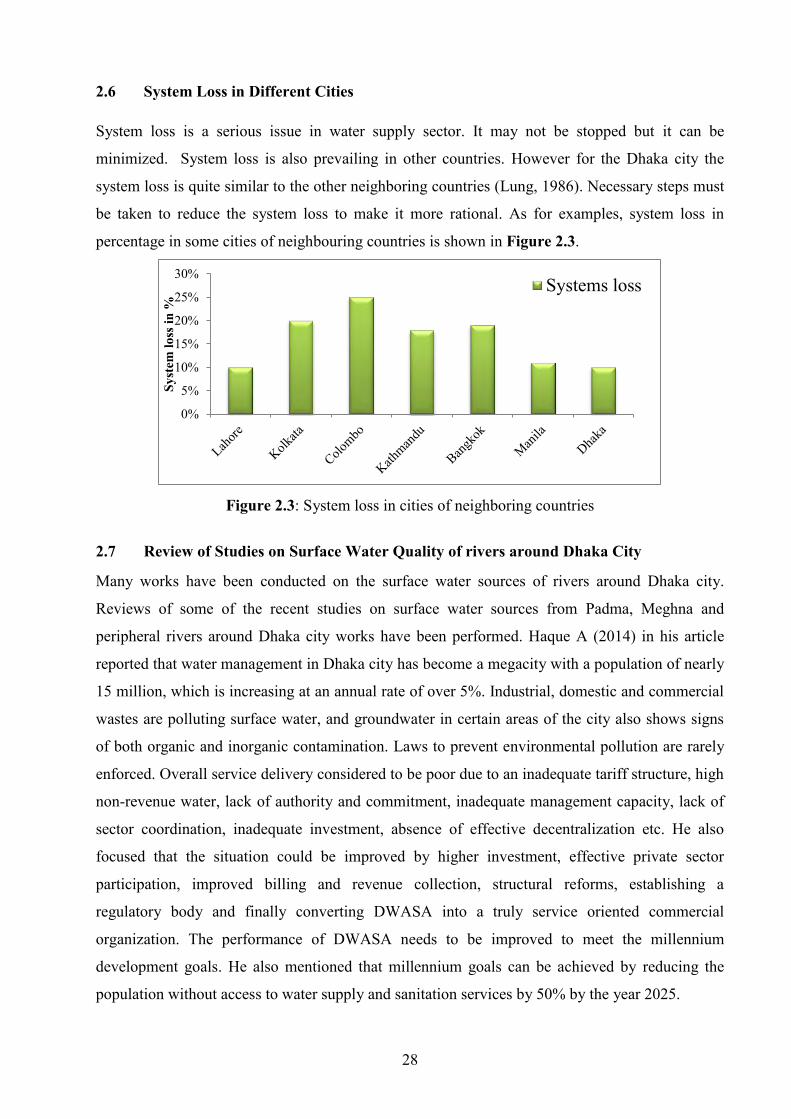
2.6 System Loss in Different Cities....................................................................... 28
2.7 Review of Studies on Surface Water Quality of rivers around Dhaka City..... 28
2.8 Review of Previous Studies on Groundwater Quality ..................................... 32
2.9 Deep Tube Wells Operated by Private Agencies .................. ......... ................... 34
2.10 Relevant Studies of Dhaka Water and Sewage Authority (DWASA)................. 34
2.11 Management Plan for Water Supply Project .................................................... 37
2.11.1 Demand and Supply Side Management .......................................................... 37
2.11.2 Water Reuse ……………………………………………………………………. 37
2.11.3 Pollution control …………………………………………………………….. 36
2.11.4 Integration of Future Sources of Supply……………………………………….. 38
2.11.5 Water Distribution System ………………………………………..……..…….. 38
2.11.6 Environmental Impact Assessment (EIA) of Industries…………..……..…….. 39
2.11.7 Enforcement of New Law: “Clean Water Act”………..……. .…… .…… .……. 39
2.11.8 Land Zoning……..……. .…… . …… .…… …… .…… …… .…… …… .……. 40
2.11.9 Coordinated Efforts ……..……. .…… . …… .…… …… .…… …… .…… …. 41
2.11.10 Maintaining ISO 14000 in industries…. .…… . …… .…… …… .…… ……. 41
2.11.11 Waste minimization in industrial processes….… . …… .…… …… .…… … 41
2.11.12 Environmental Monitoring Program ….… . …… .…… …… …… .…… …. 42
2.11.13 Clean-Up of Contaminated River Beds ….… . …… .…… …… …… .…… 42
2.11.14 Rainwater Harvesting ...................................................................................….. 43
2.11.15 Institutional Responsibilities … . …… .…… …… …… . ……………….. 43
2.12 Concluding Remarks………………………………………………………. ….. 44
CHAPTER 3 METHODOLOGY ………………………….……………………… 45
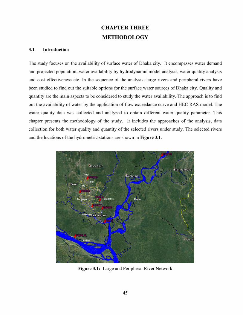
3.1 Introduction ………………………………………………………………… 45
3.2 Methodology ………………………………………………………………… 46
3.2.1 Population Prediction and Assessment of Water Demand…………………… 46
3.2.2 Water Quality Analysis ……………………………………………………… 47
3.2.3 Ground Water Data …………………………………………………………… 50
3.2.4 River Data …………………………………………………………………… 50
3.2.4.1 Bathymetry …………………………………………………………………… 50
3.2.4.2 Water Level and Discharge …………………………………………………… 50
Page 11
viii
3.2.5 Analysis of Water Availability ……………………………………………….. 51
3.2.5.1Application of Mathematical Model…………………………………………… 51
3.2.5.2 Model Calibration and Validation …………………………………………… 52
3.2.5. Analysis for Surface Water Withdrawal ……………………………………… 52
3.2.6. Evaluation of Sources ………………………………………………………… 53
3.3 Flow Diagram Showing Overall Methodology of the Study ………………… 53
3.4 Concluding Remarks ………………………………………………………… 56
CHAPTER 4 ASSESSMENT OF FUTURE WATER DEMAND 57
4.1 Introduction………………………………………………………………......... 57
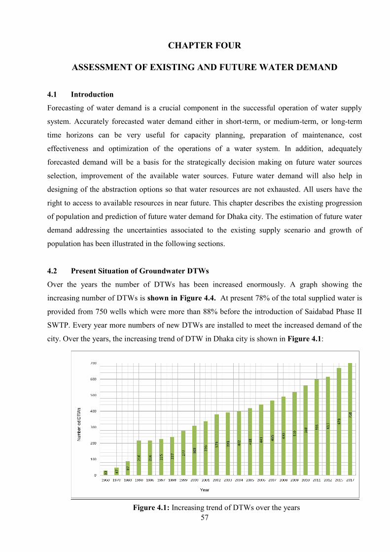
4.2 Present Situation of Groundwater DTWs ………………………………........ 57
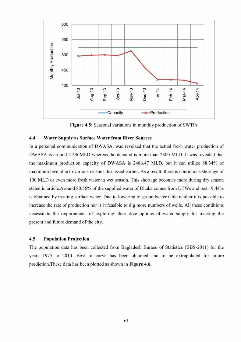
4.3 Surface Water Treatment Plants (SWTP) Operated by DWASA.....…….......... 60
4.4 Water Supply as Surface Water from River Sources..... ..... .....…….............. 61
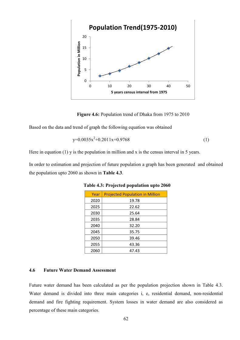
4.5 Population Projection..... ..... .....… …......…......…......…......…......….............. 61
4.6 Future Water Demand Assessment…......…......…......…......…......….............. 62
4.6.1 Residential Water Demand …......…......…......…......…......…......….............. 63
4.6.2 Non Residential Water Demand …......…......…......…......…......…......…........ 63
4.6.3 Total Future Water Demand …......…......…......…......…......…......….............. 63
4.7 Concluding Remarks …......….....…......…......…......…......…......….............. 66
CHAPTER 5 ASSESSMENT OF WATER QUALITY ………………………………… 67
5.1 General …………………..……………………………..………………….. 67
5.2 Water Quality Parameters ………………………………………………… 67
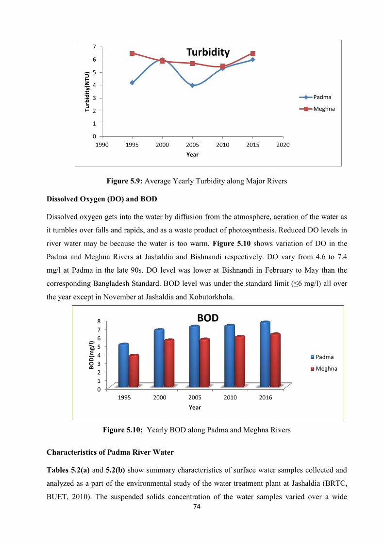
5.3 Water Quality Padma and Meghna Rivers ……………………………….. 68
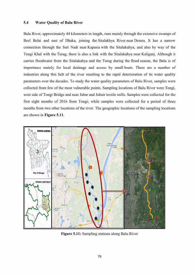
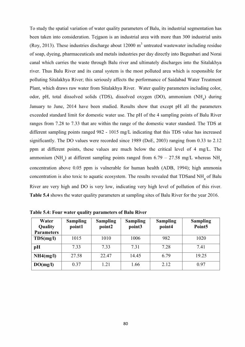
5.4 Water Quality of Balu River ........................................................................ 79
5.5 Water Quality of Sitalakhya River .............................................................. 84
5.6 Water Quality of Turag River ................................................................... 89
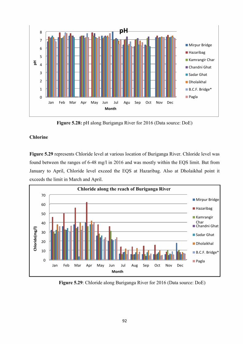
5.7 Water Quality of Buriganga River ............................................................. 90
5.8 Water Quality of Dhaleshwari River ........................................................ 95
5.9 Yearly Variation of Water Quality Parameters of the River System ………. 96
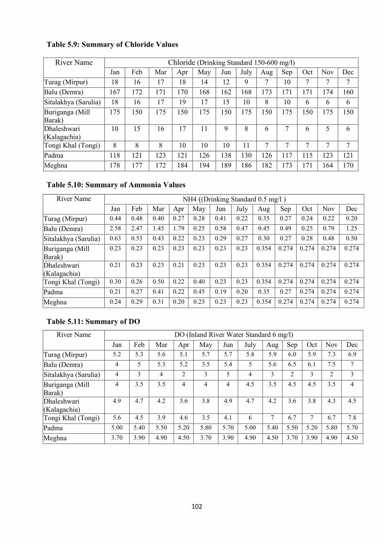
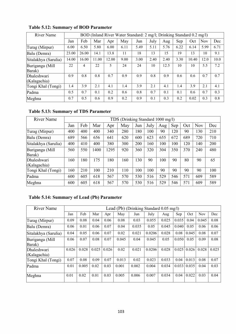
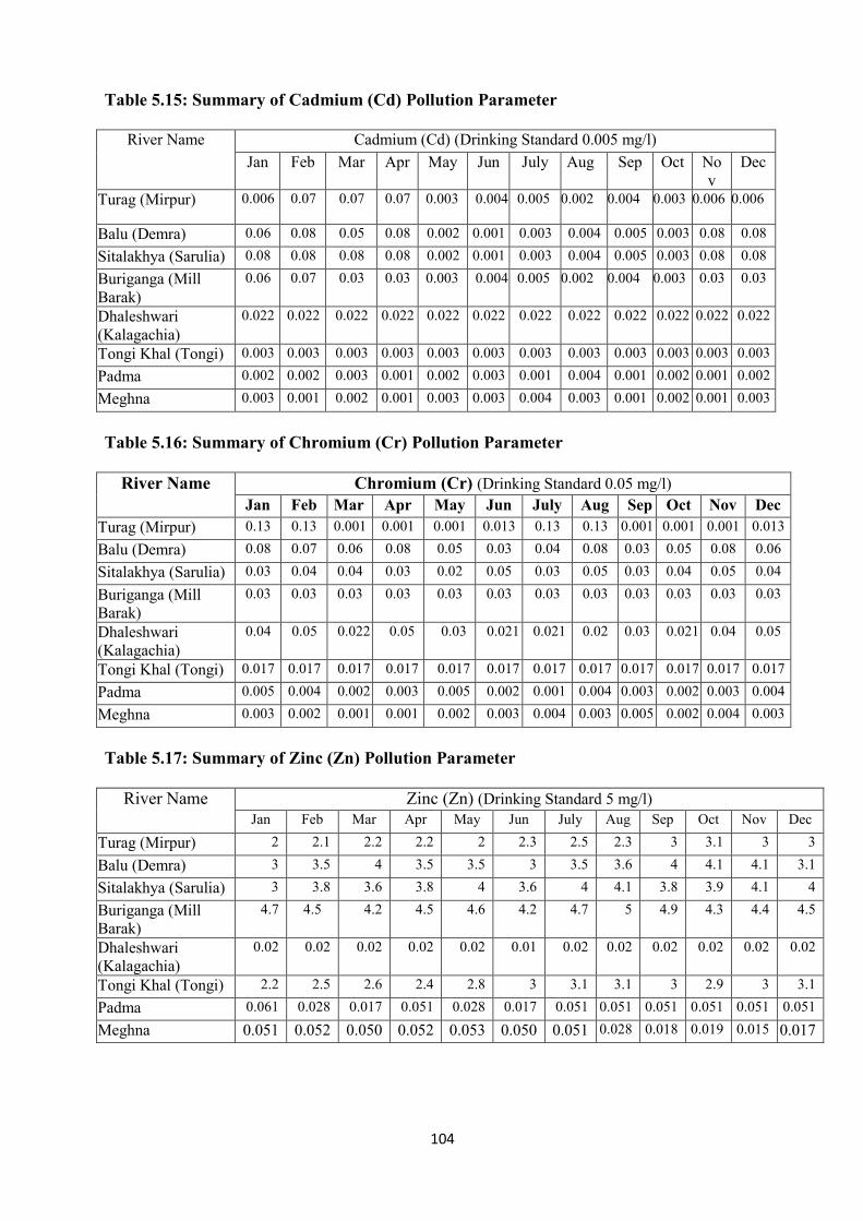
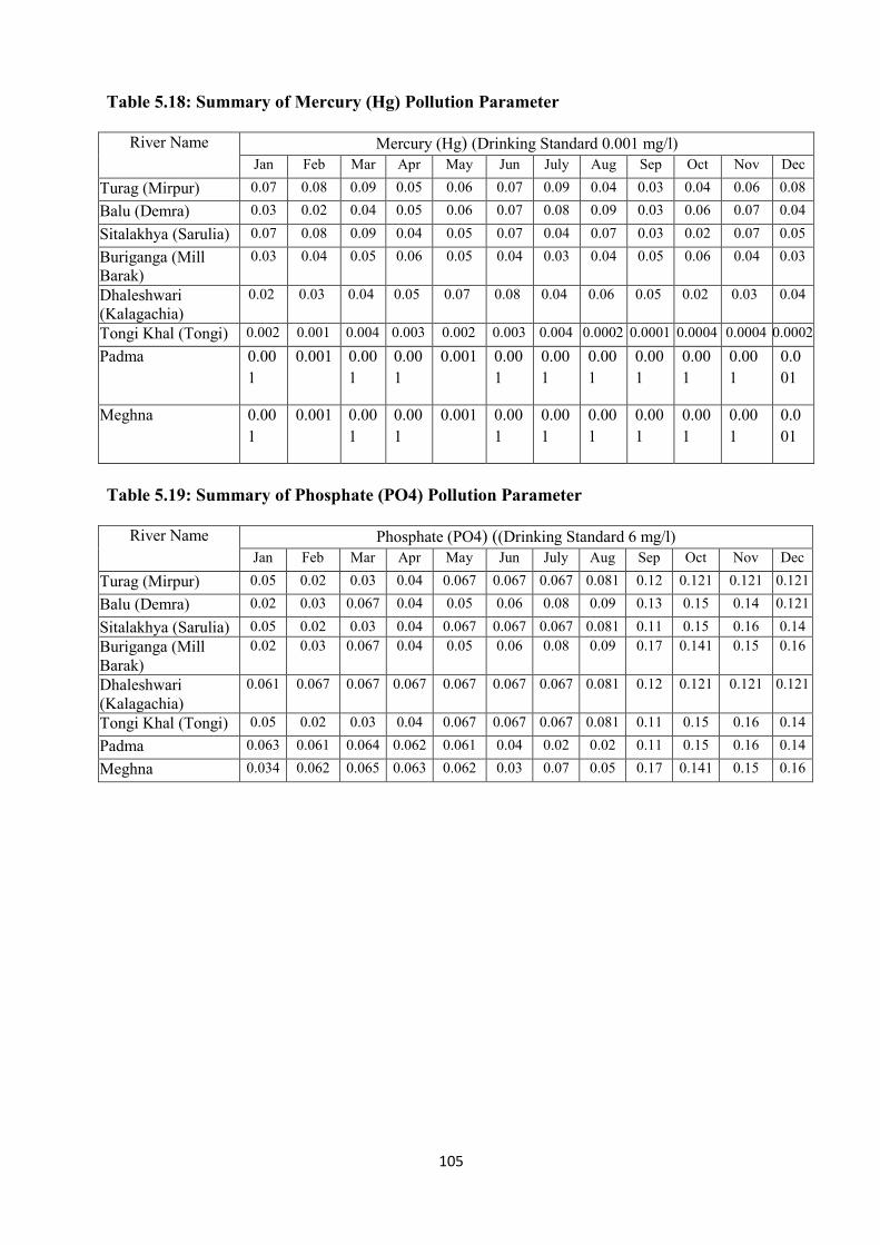
5.10 Summary of Pollutant Loading of Surface Water System of Dhaka City .... 102
Page 12
ix
5.11 Collection and Analysis of Water Samples..................... ……….……. 105
5.12 Summary and Concluding Remarks……………………………….……. 107
CHAPTER 6 ANALYSIS OF SURFACE WATER AVAILABILITY……………...... 111
6.1 Introduction ………………………………………………………………... 111
6.2 Description of Selected River Sources for Surface Water .………….......... 111
6.3 Peripheral Rivers and Major Rivers for Water Availability ……………… 113
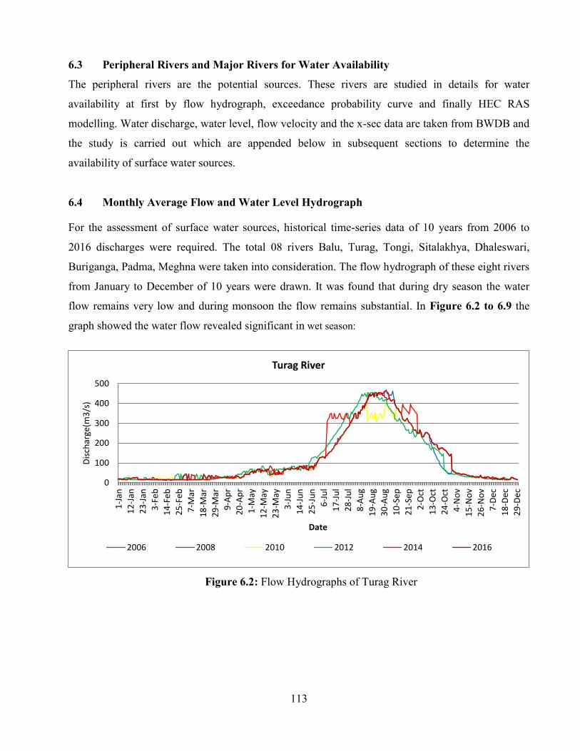
6.4 Monthly Average Flow and Water Level Hydrograph ………………….. . 113
6.5 Environmental Flow Estimation …………………………….........……… 122
6.5.1 Assessment of 10% Mean Annual Flow ...................................................... 122
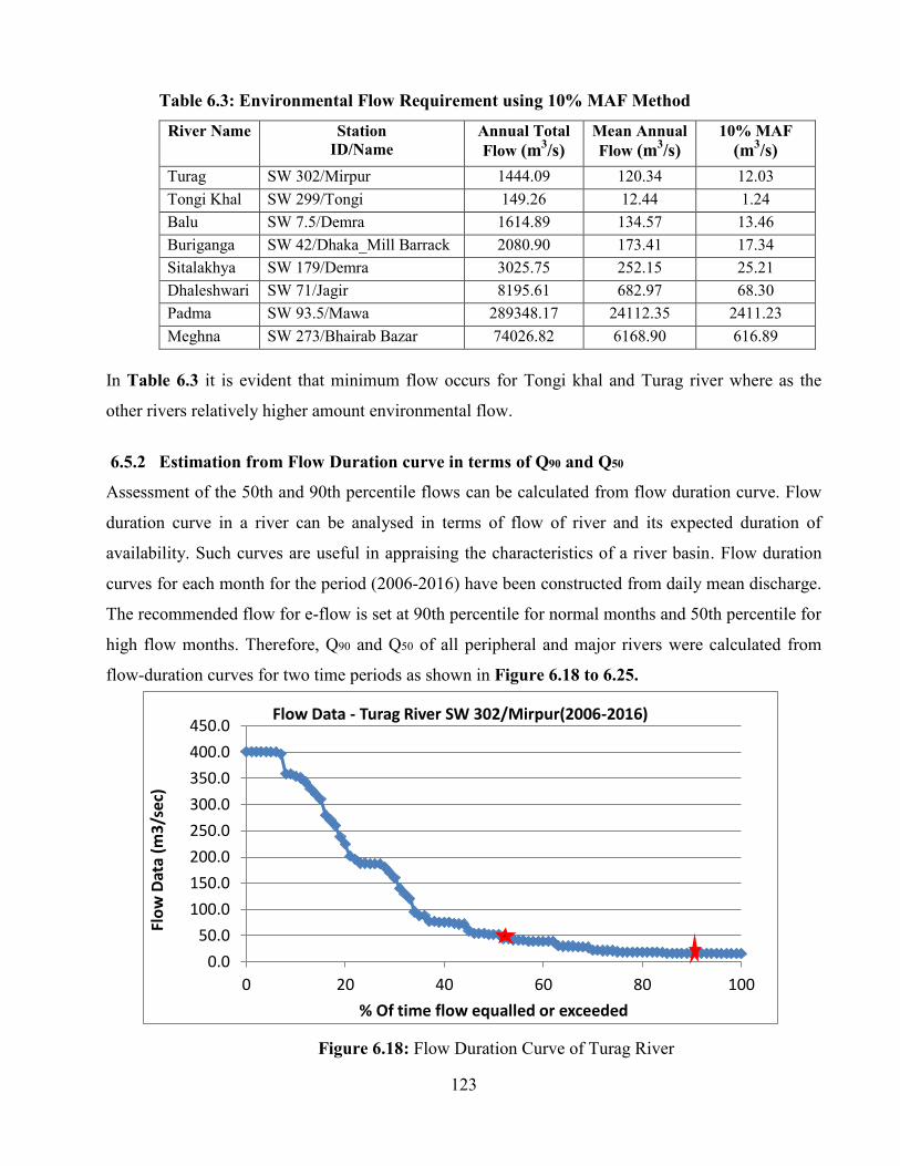
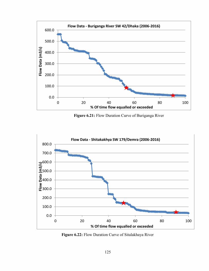
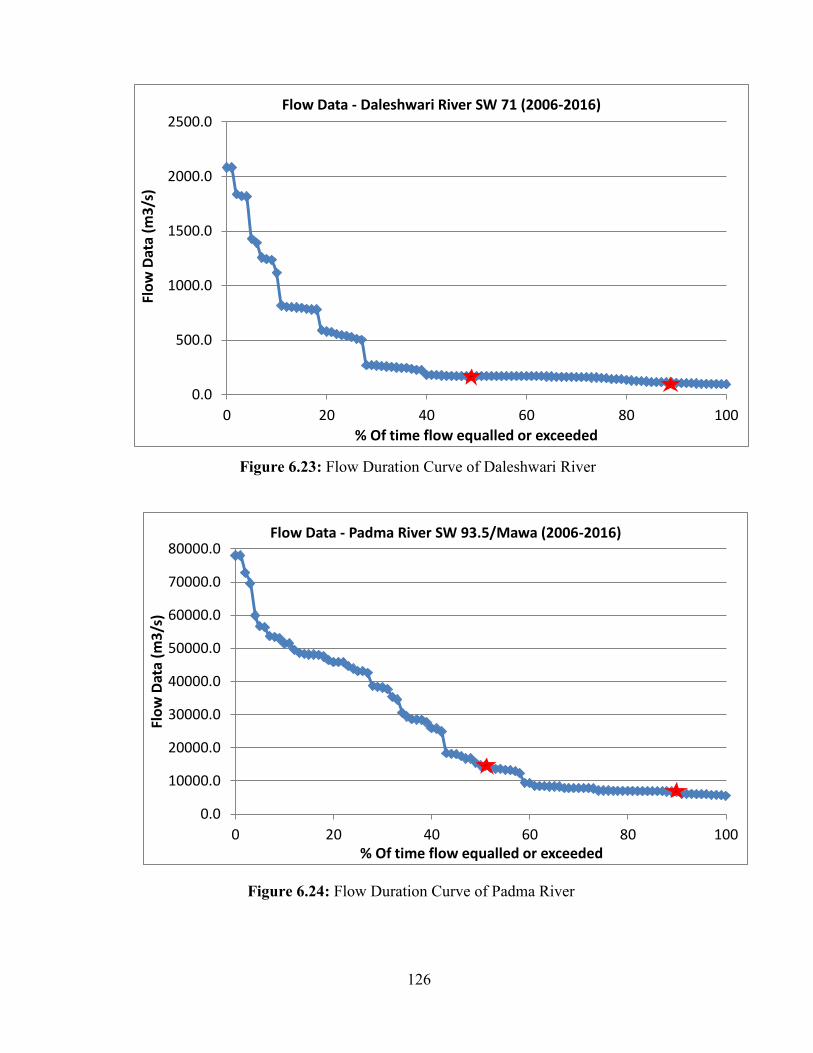
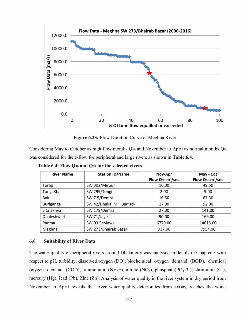
6.5.2 Estimation from Flow Duration curve in terms of Q90 and Q50 ....... ........ 123
6.6 Suitability of River Data ……………………………………………. 128
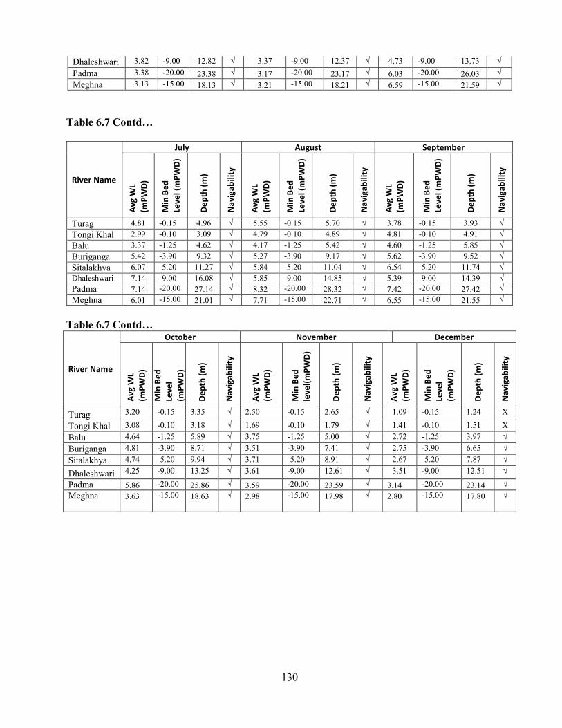
6.7 Navigability ………………………………………………………….……. 127
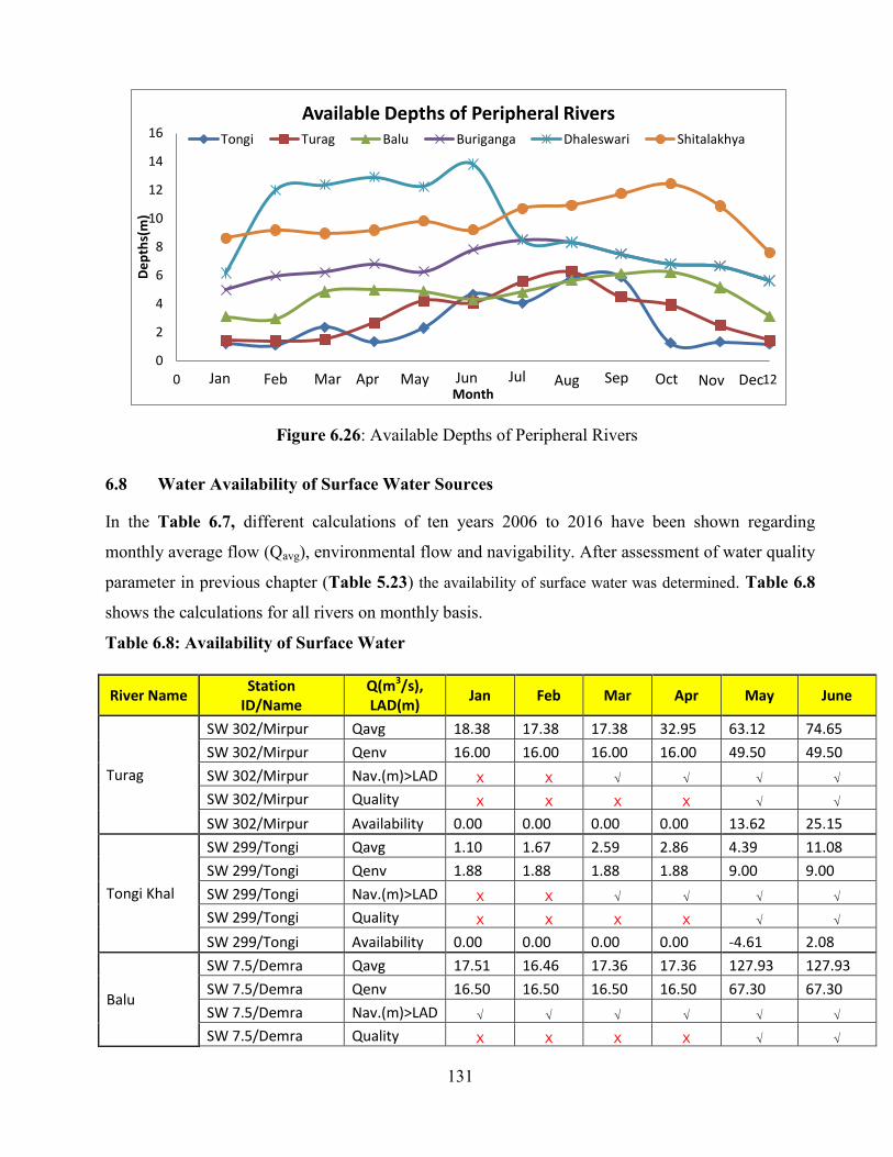
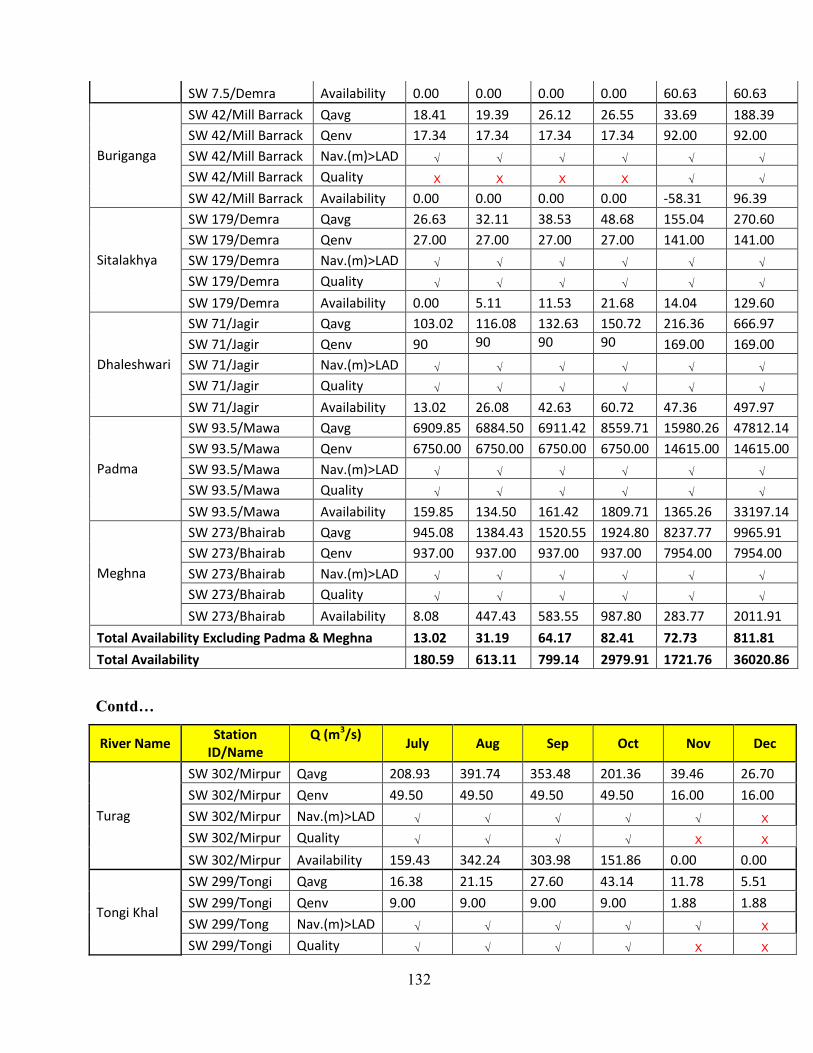
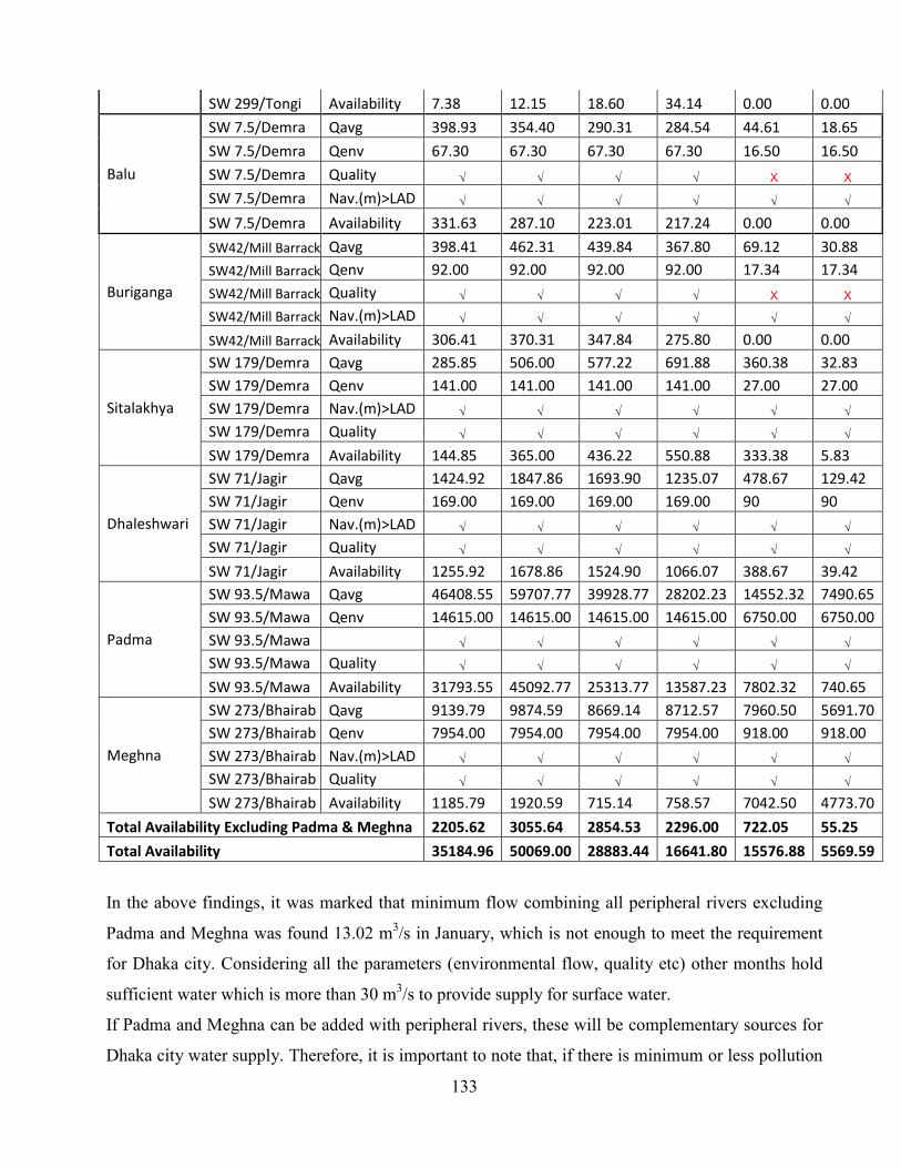
6.8 Water Availability of Surface Water Sources ……………………………. 131
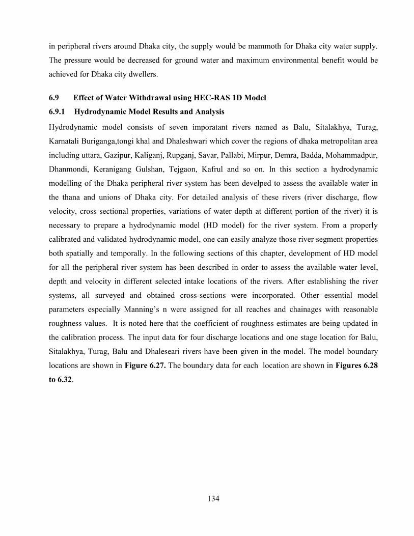
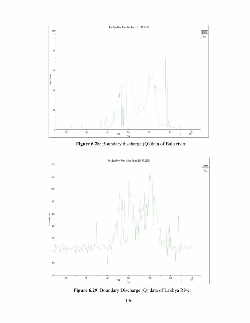
6.9 Effect of Water Withdrawal using HEC RAS 1D Model …………….… 134
6.9.1 Hydrodynamic Model Results and Analysis …………………………….. 134
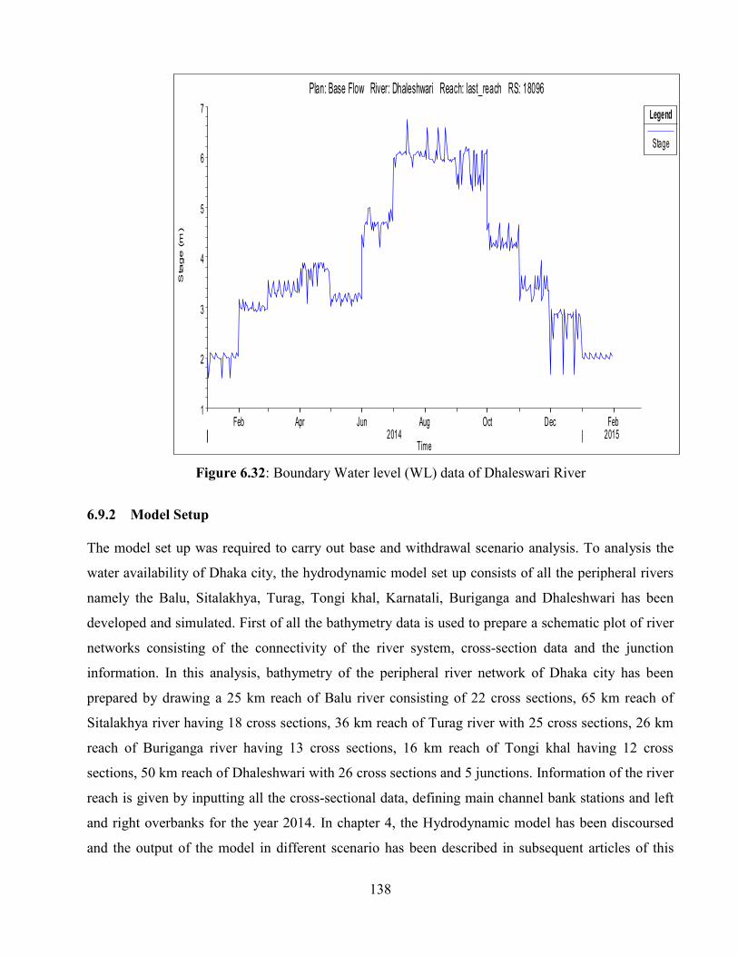
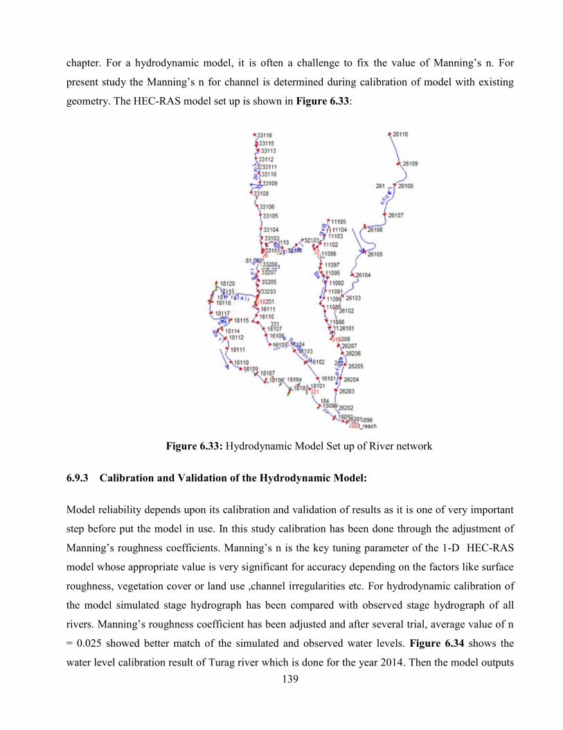
6.9.2 Model Setup ……………………………………………………..………. 138
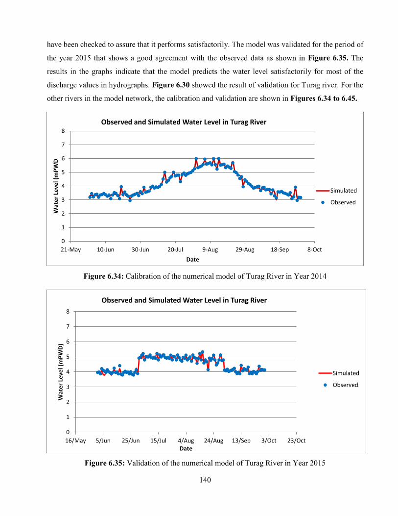
6.9.3 Calibration and Validation of the Hydrodynamic Model:……………….... 139
6.9.4 Model Results for Various Abstraction Scenarios………………………… 145
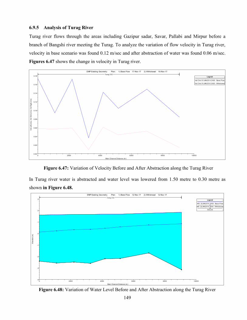
6.9.5 Analysis of Turag River ………………………………………..………… 149
6.9.6 Analysis of Tongi Khal ……………………………..…………………….. 150
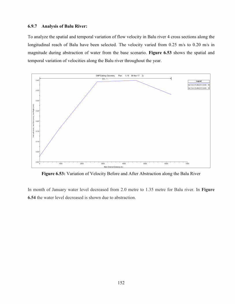
6.9.7 Analysis of Balu River ……………………………….………………….. 152
6.9.8 Analysis of Buriganga River ........................................................................ 153
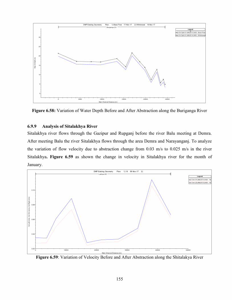
6.9.9 Analysis of Sitalakhya River.................................................................... 155
6.9.10 Analysis of Dhaleswari River ..................................................................... 157
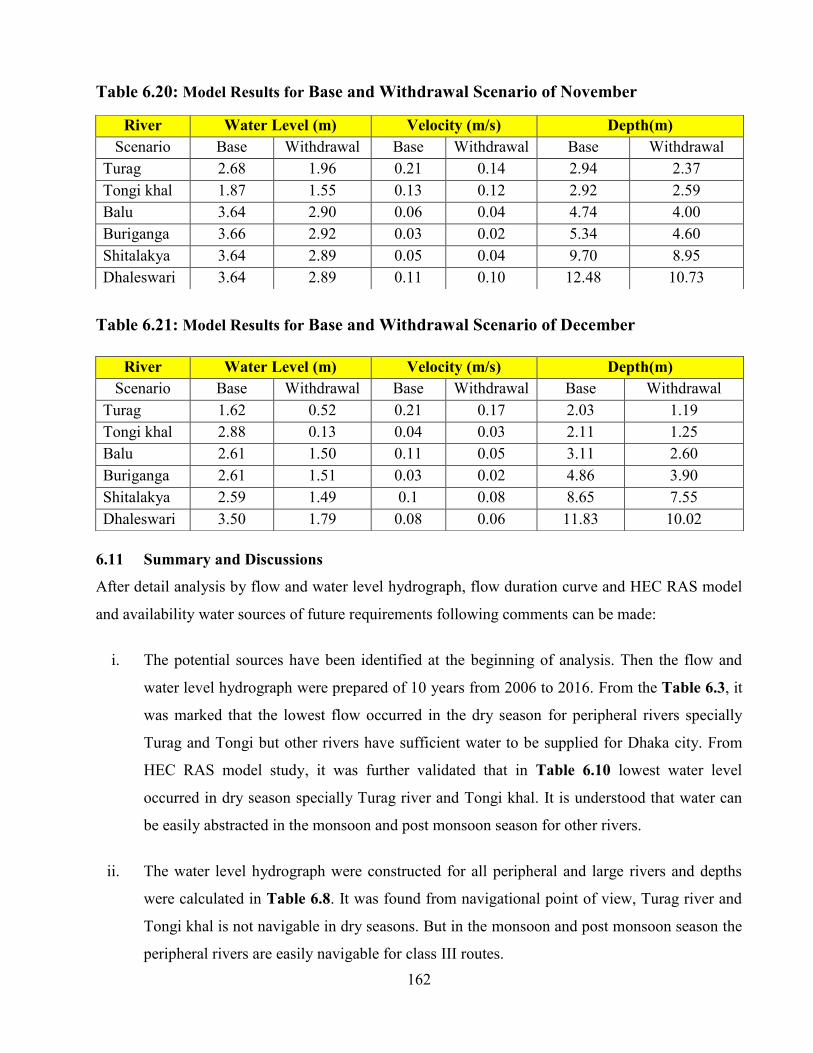
6.10 Summary Results of the Base and Withdrawal Scenario ............................ 158
6.11 Summary and Discussions ........................................................................... 162
CHAPTER 7 EVALUATION OF SURFACE WATER SOURCES FOR DHAKA CITY 165
7.1 General………………………………………………………………….. 165
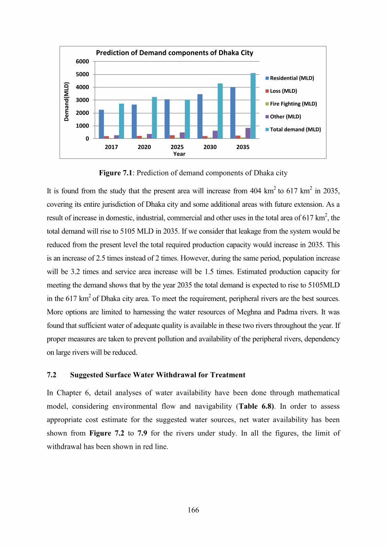
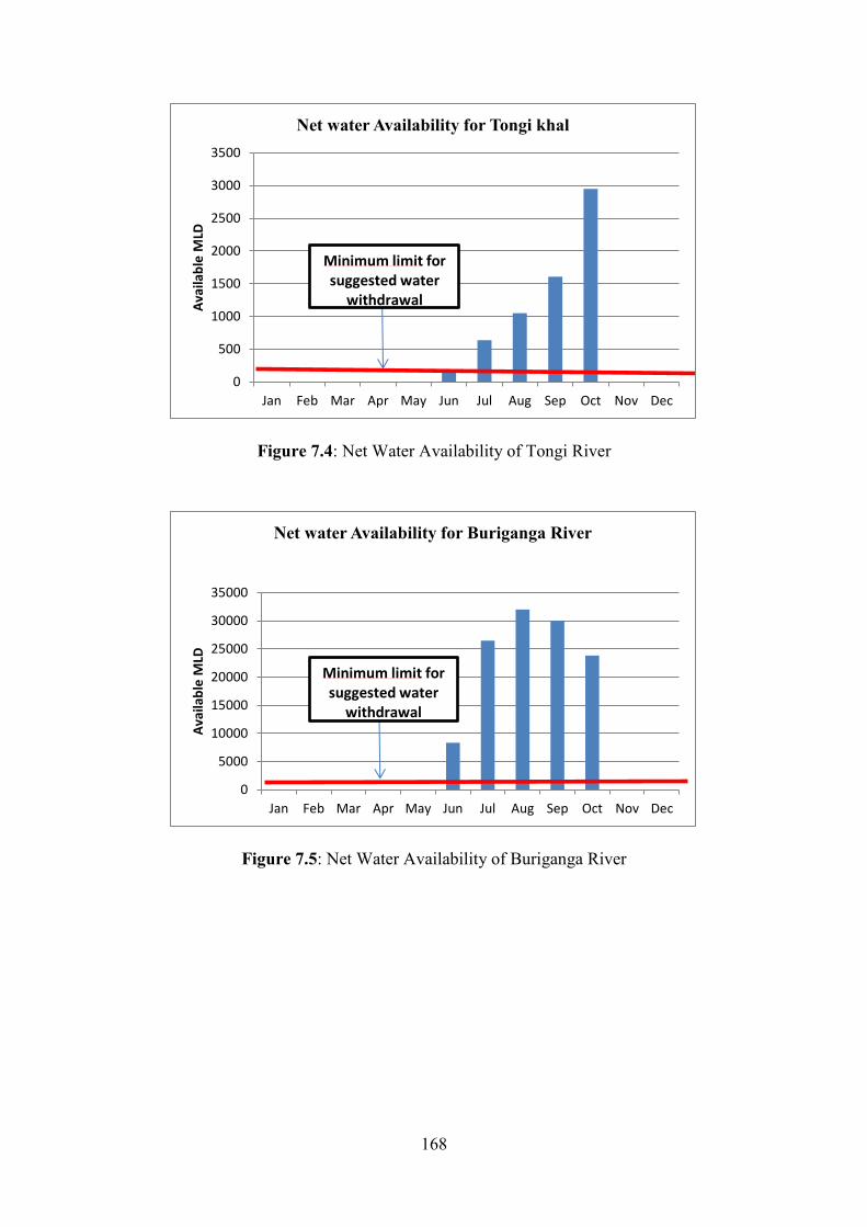
7.2 Suggested Surface Water Withdrawal for Treatment ……………………….. 166
7.3 Evaluation Criteria ......................……………………………………………… 171
7.3.1 Water Quality of Peripheral Rivers…………………………………………… 171
Page 13
x
7.3.2 Water Quality of Large Rivers………………………………………………… 172
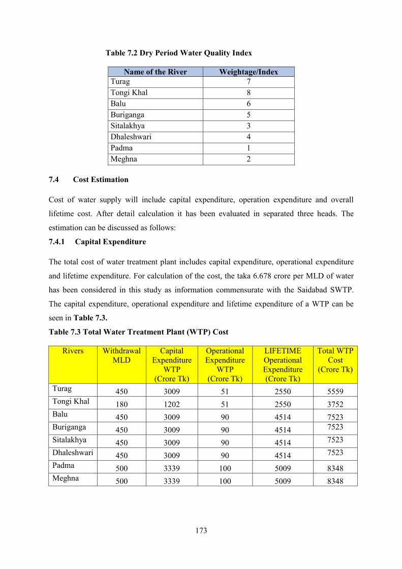
7.4 Cost Estimation ……………………………………………………………… 173
7.4.1 Capital Expenditure …………………………………………………………… 173
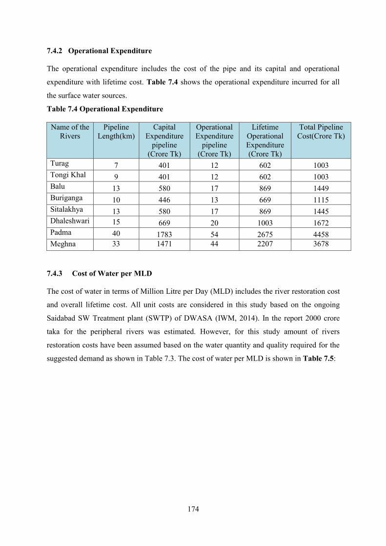
7.4.2 Operation Expenditure………………………………………………………… 174
7.4.3 Cost of Water per MLD………………………………………………………. 174
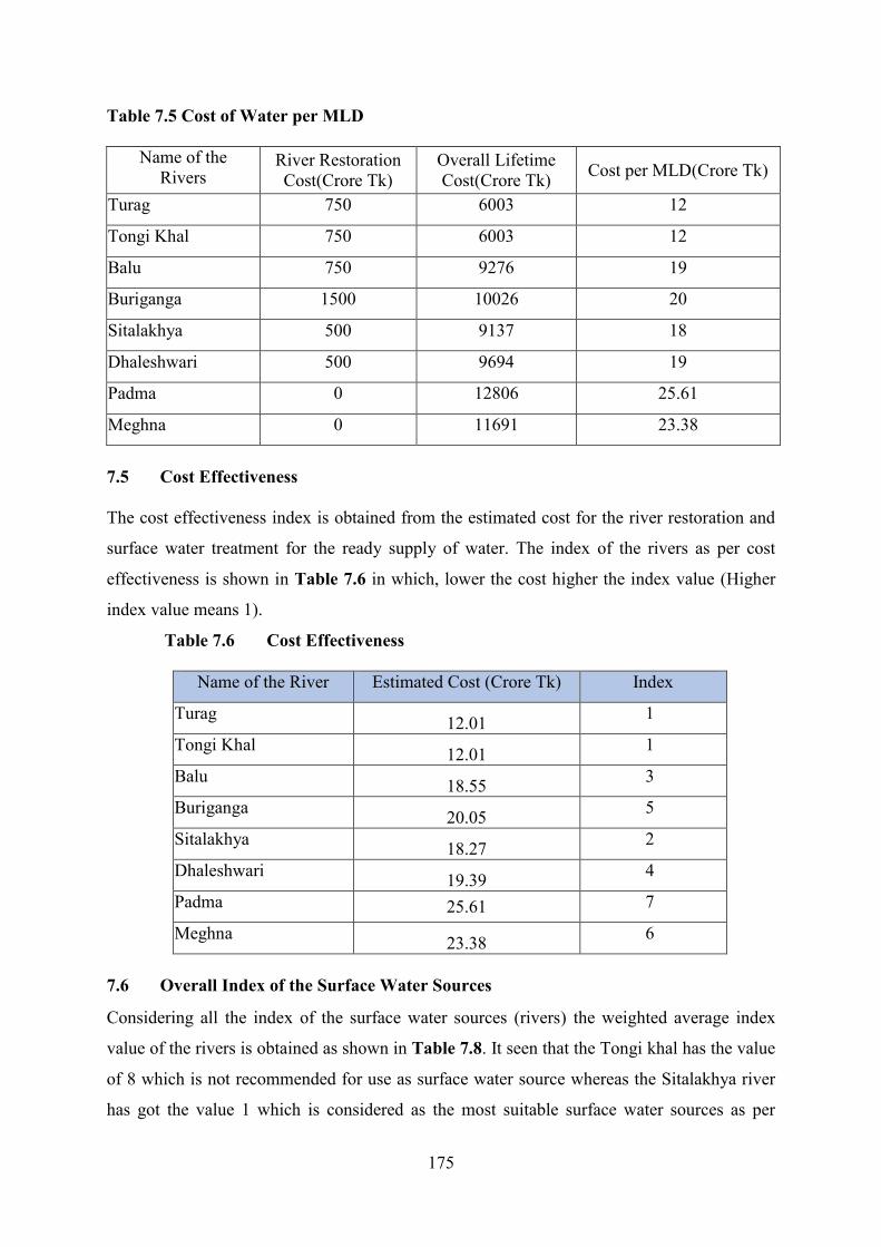
7.5 Cost Effectiveness ………………………………………………………….... 175
7.6 Overall Index of the Surface Water Sources………………………………… 175
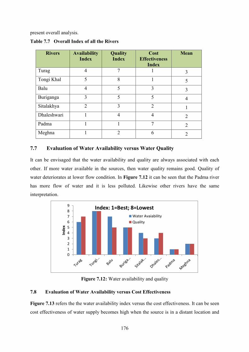
7.7 Evaluation of Water Availability versus Water Quality……………........... . 176
7.8 Evaluation of Water Availability versus Cost Effectiveness……………….. 176
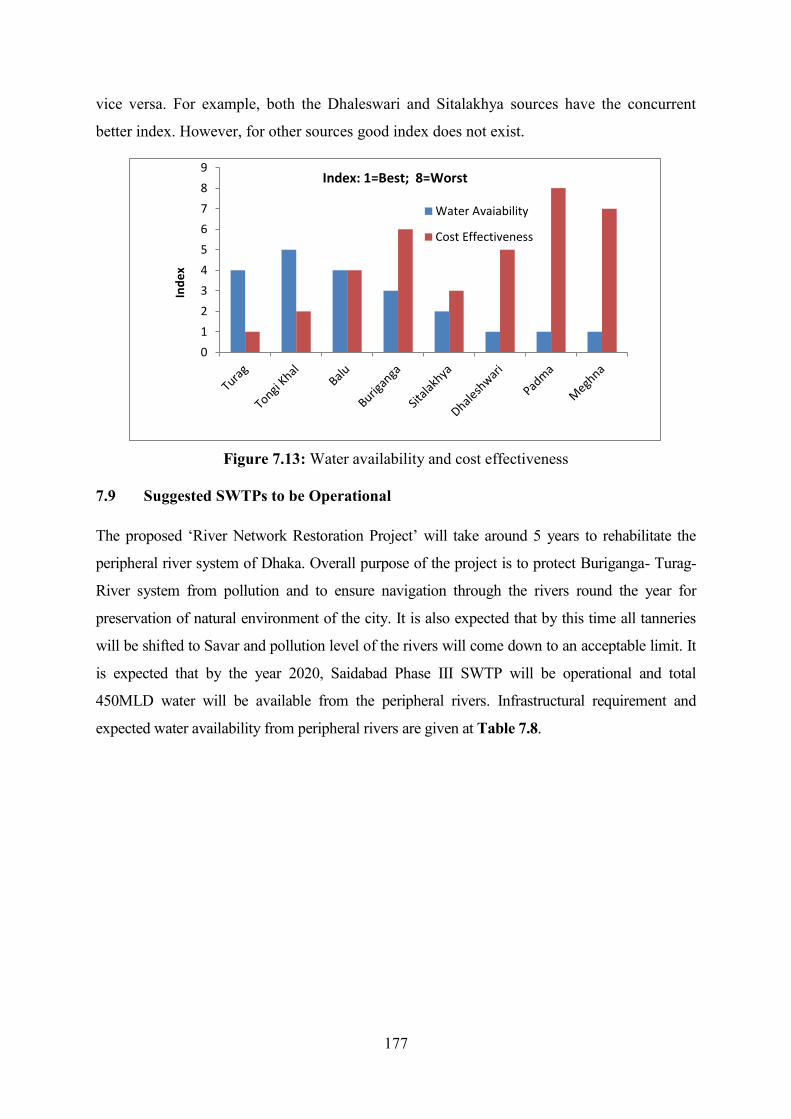
7.9 Suggested SWTP to be Operational…………………….……….…….……… 177
7.9.1 Utilization of Large Rivers ……………….………………….……………… 178
7.9.2 Paradigm Shifting towards Surface Water Sources ....................................... 179
7.10 Financial Plan ................................................................................................. 180
7.11 Concluding Remarks.…….…….… ….….…….….…….….…….….…..…. 180
CHAPTER 8 CONCLUSIONS AND RECOMMENDATIONS ……………………… . 182
8.1 General…………………………………..……………………………........ 182
8.2 Conclusions……………………………..……………………………......... 182
8.3 Recommendations for Future Study …………………………………….... 185
REFERENCES……………………………………………………………………………… 186
Page 14
xi
LIST OF FIGURES Figure 1.1 Water Supply Sources of Dhaka City ……………………..………………... 3
Figure 1.2 Peripheral Rivers around Dhaka City ………………………..………………... 4
Firure 1.3 Field Survey for Demand and Supply ………………………………… 5
Figure 1.4 Map of Study Area …………….…………………………………….……… 7
Figure 2.1 Diagram showing the coherence in plans and policy……………………….. 26
Figure 2.2 Water Supply Scenario in different cities ………….……………………….. 27
Figure 2.3 System loss in cities of neighboring countries ………….……………………….. 28
Figure 3.1 Large and Peripheral River Network.................................................................. 45
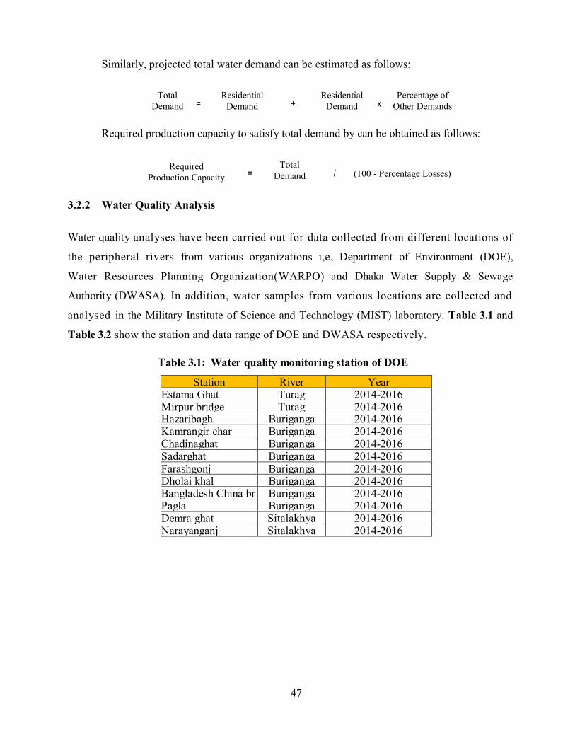
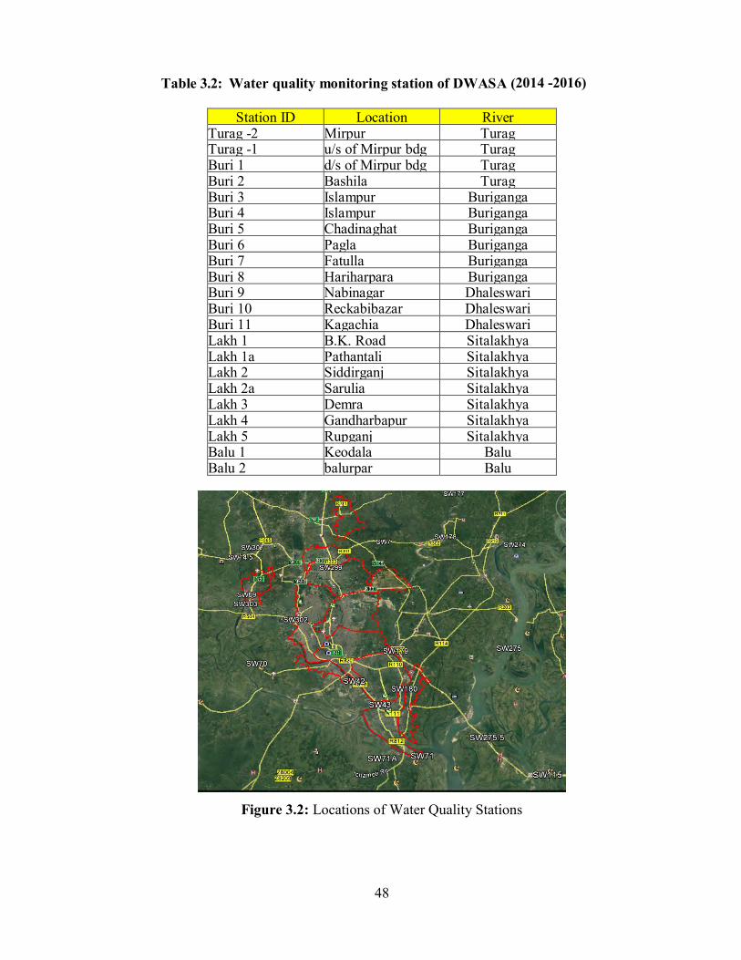
Figure 3.2 Locations of Water Quality Stations................................................................. 40
Figure 3.3 Water Samples from Rivers in September 2017.............................................. 49
Figure 3.4 Water Samples from Rivers in January 2018...................................................... 49
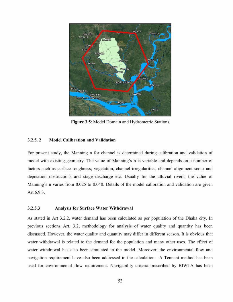
Figure 3.5 Model Domain and Hydrometric Stations...................................................... 44
Figure 3.6 Flow Diagram of Evaluating the Sources............. ................................................ 53
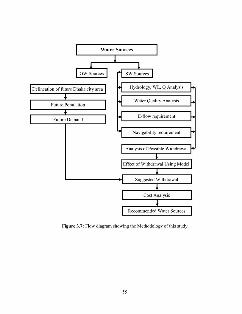
Figure 3.7 Flow diagram showing the Methodology of this study ........................................ 55
Figure 4.1 Increasing trend of DTWs over the years …………………..……… 57
Figure 4.2 Gradual increase in mining depth of DTWS …..……………………………. 58
Figure 4.3 Groundwater depletion state in Lalbagh, Motijheel and Cantonment ……. 59
Figure 4.4 Groundwater depletion state in Tejgaon, Gulshan and Dhanmondi………… 59
Figure 4.5 Seasonal variations in monthly production of SWTPs………………… …… 61
Figure 4.6 Population trend of Dhaka from 1975 to 2010 .…..………………….............. 62
Figure 4.7 Map showing population density of Dhaka city.…….…… …………………. 64
Figure 5.1 Sampling Locations of Padma River on Google Earth ................................. …….. 69
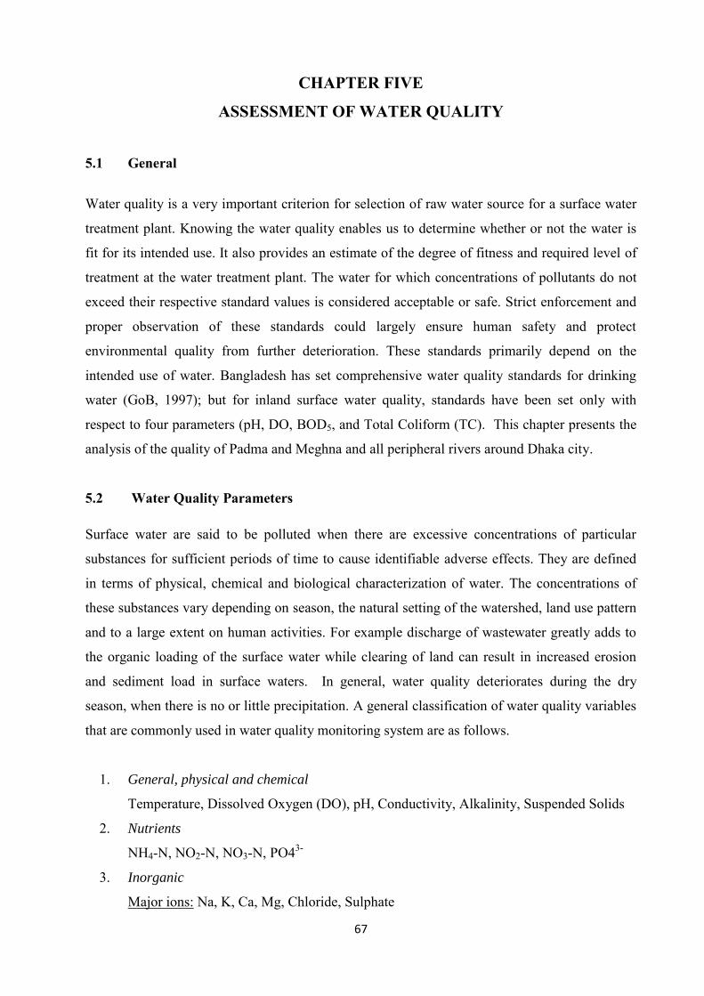
Figure 5.2 Sampling Locations of Meghna River on Google Earth ................................ 70
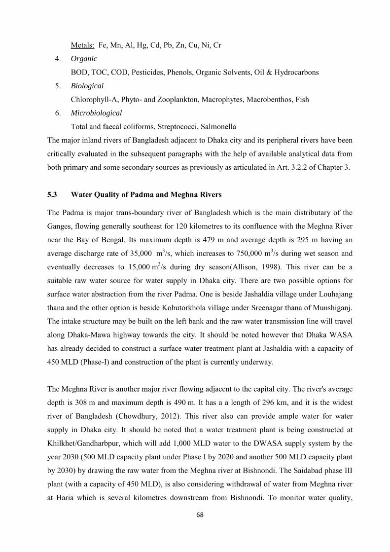
Figure 5.3 pH along Padma River for the year 2015 (Data source: WARPO) ................ 70
Figure 5.4 pH along Meghna River for the year 2016 .. ....... ....... ....... ....... ....... .............. 71
Figure 5.5 EC along Padma and Meghna Rivers at Jashaldia and Bishnandi. ....... .............. 72
Figure 5.6 Monthly EC along Major Rivers at sampling points. ....... .............. ....... .............. 72
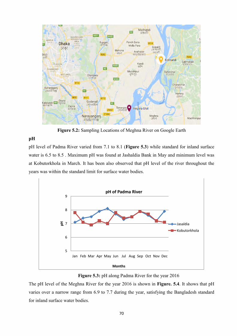
Figure 5.7 Chloride concentration along Major Rivers at Jashaldia and Bishnandi. ....... ....... 73
Figure 5.8 Chloride concentration along Major Rivers in 2016. ....... . ....... . ....... . .............. 73
Figure 5.9 Average Yearly Turbidity along Major Rivers .. ..... . ..... ........ . ....... . .............. 74
Figure 5.10 Yearly BOD along Padma and Meghna Rivers.. ..... . ..... ........ . ....... . .............. 74
Figure 5.11 Sampling stations along Balu River.. ..... . ..... ........ . ....... . .............. ....... . ......... 79
Page 15
xii
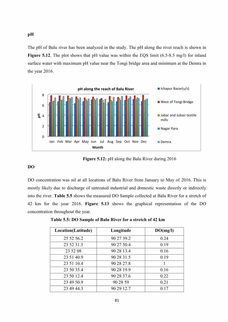
Figure 5.12 pH along the Balu River.. ..... . ..... ........ . ....... . ............ ............ ............ . . ......... 81
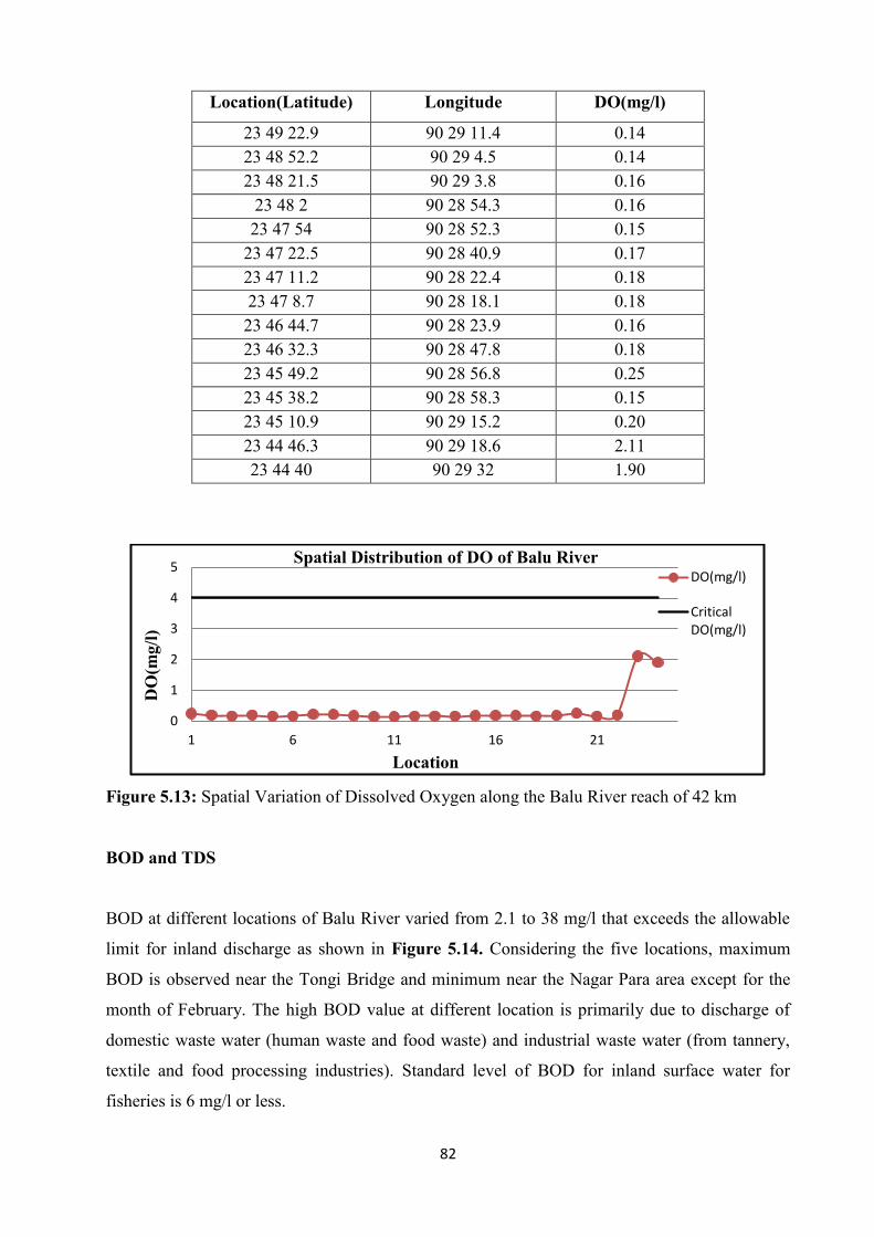
Figure 5.13 Spatial Variation of Dissolved Oxygen along the Balu River reach of 42 km…... 82
Figure 5.14 BOD along the Balu River ……………………………………………………….. . 83
Figure 5.15 TDS along the Balu River ………………………………………………………. 83
Figure 5.16 Chloride (top) along the Balu River………………………………………………. 84
Figure 5.17 Water Quality Sampling Stations for Sitalakhya River …………………………. 85
Figure 5.18 pH of Sitalakhya River for the year 2016……………………………… …..……. 85
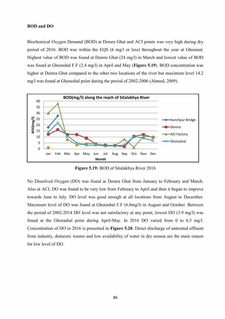
Figure 5.19 BOD of Sitalakhya River 2016……………………………… …..……. …..…… 86
Figure 5.20 DO concentration of Sitalakhya River for 2016..…………… …..……. …..…… 87
Figure 5.21 Turbidity of Sitalakhya River for the year 2016..…………… …..……. …..…… 87
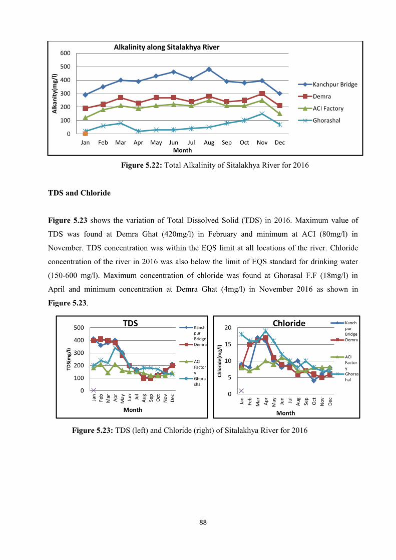
Figure 5.22 Total Alkalinity of Sitalakhya River for 2016..…………… …..………. …..…… 88
Figure 5.23 TDS (left) and Chloride (right) of Sitalakhya River for 2016…..………. …..…… 88
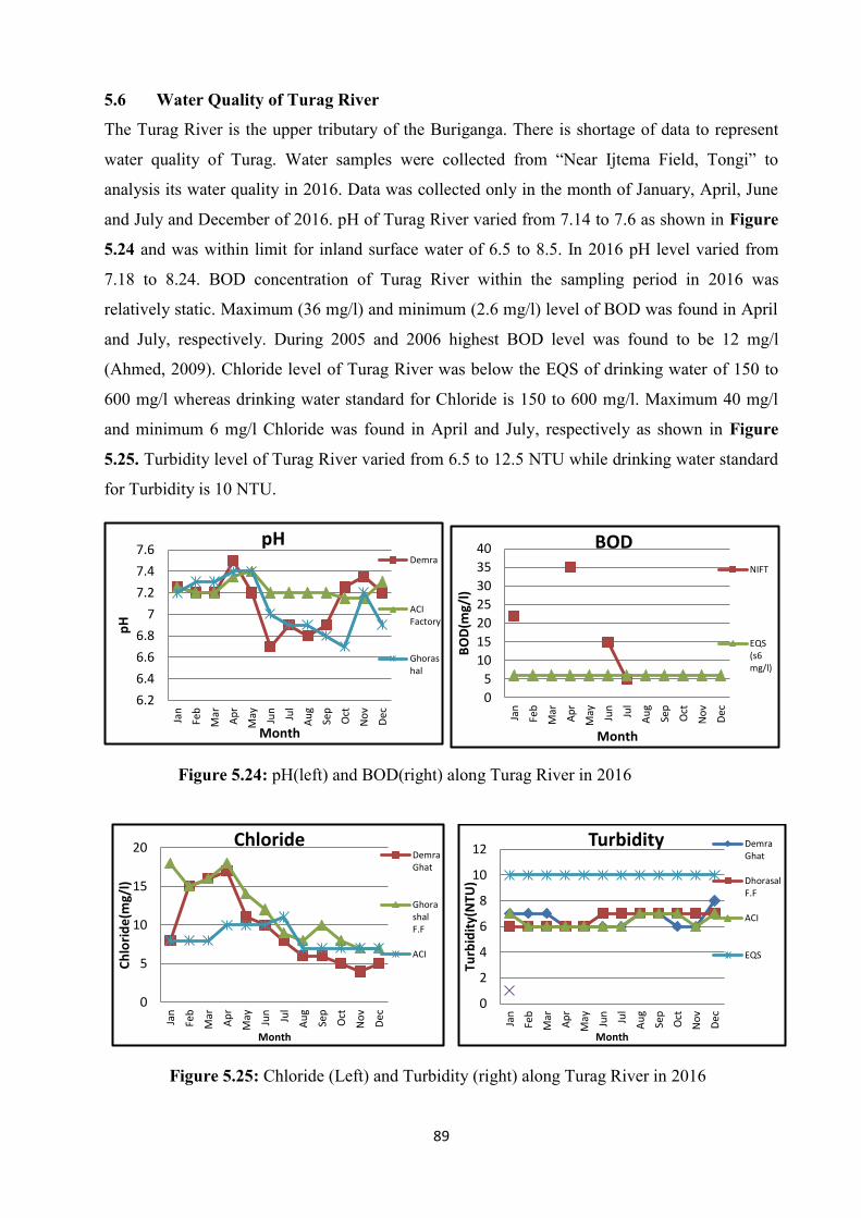
Figure 5.24 pH(left) and BOD(right) along Turag River in 2016…..……..……..……. …..… 89
Figure 5.25 Chloride (Left) and Turbidity (right) along Turag River in 2016…...……. …..……89
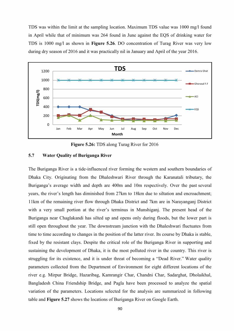
Figure 5.26 TDS along Turag River in 2016…...…...…...…...…...…...…...…...……. …..……. 90
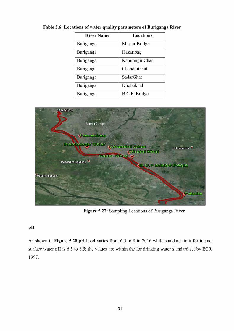
Figure 5.27 Locations of Buriganga River …...…...…...…...…...…...…...…...………. …..…… 91
Figure 5.28 pH along Buriganga River for 2016...…... ...…... ...…...…...…...………. …..…… 92
Figure 5.29 Chloride along Buriganga River in 2016...…... ...…... ...…...…..………. …..…….. 92
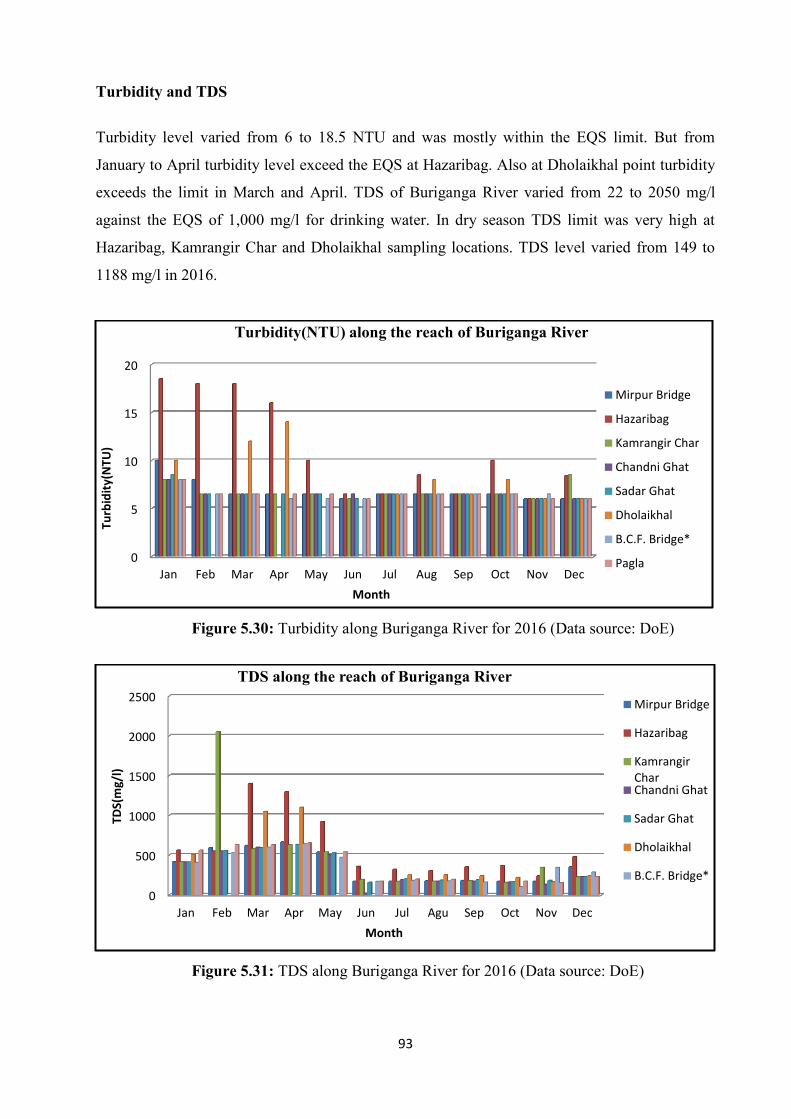
Figure 5.30 Turbidity along Buriganga River for 2016...…... ...…... ...…...…..………. …….….93
Figure 5.31 TDS along Buriganga River for 2016...…... ...…... ...…...….. ……………. …….…93
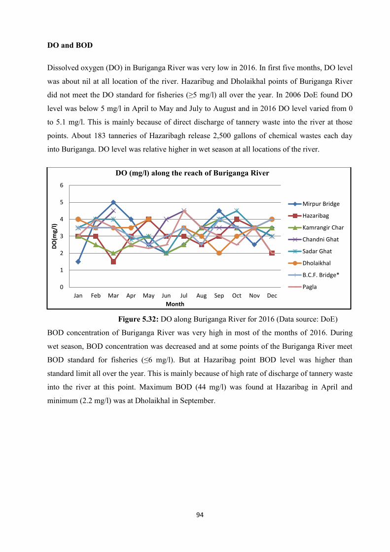
Figure 5.32 DO along Buriganga River for 2016...…... ...…... ...…...….. ……………. …….….94
Figure 5.33 BOD along Buriganga River for 2016...…... ...…... ...…...….. ……………. ………95
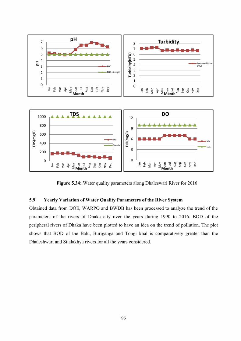
Figure 5.34 Water quality parameters along Buriganga River for 2016.….. …………… …….. 96
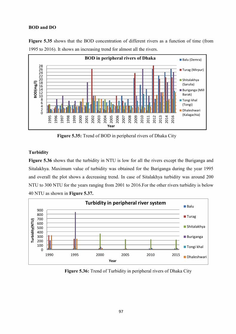
Figure 5.35 Trend of BOD in peripheral rivers of Dhaka City.….. …………… ………… … 97
Figure 5.35 Trend of DO in peripheral rivers of Dhaka City.… .. …………… ………… … 97
Figure 5.37 Trend of Turbidity in peripheral rivers of Dhaka City .................................... 98
Figure 5.38 Trend of pH in peripheral rivers of Dhaka City ............................................... 98
Figure 5.39 Trend of Chloride in peripheral rivers of Dhaka City ...................................... 99
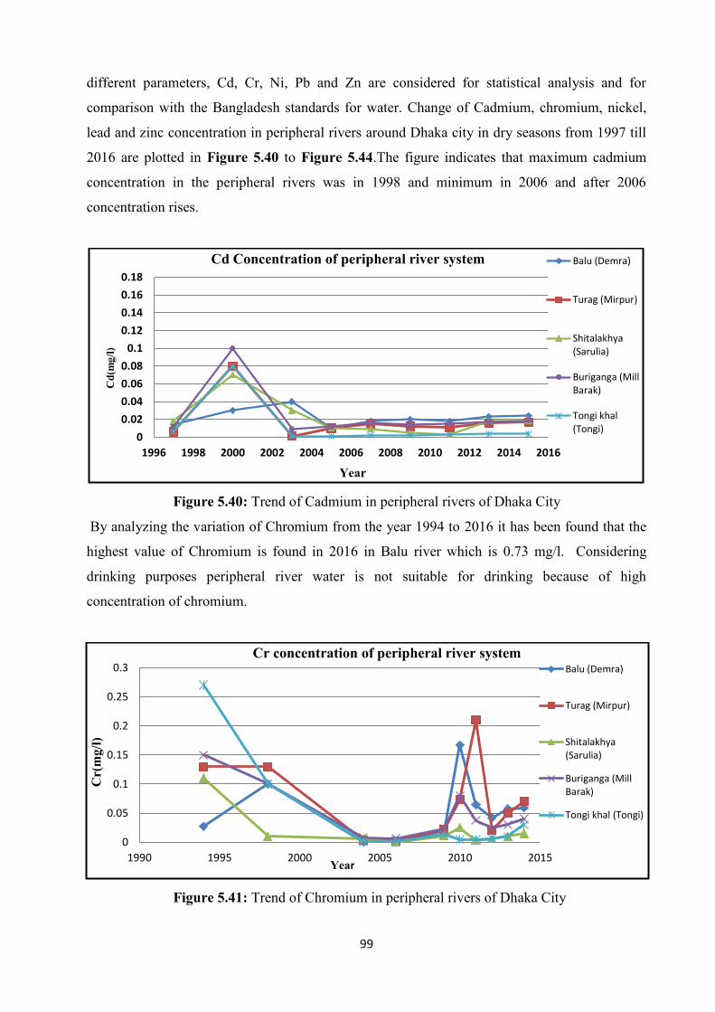
Figure 5.40 Trend of Cadmium in peripheral rivers of Dhaka City ..................................... 100
Figure 5.41 Trend of Chromium in peripheral rivers of Dhaka City ................................... 100
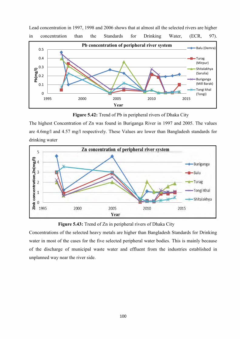
Figure 5.42 Trend of Pb in peripheral rivers of Dhaka City ................................................. 101
Figure 5.43 Trend of Zn in peripheral rivers of Dhaka City ................................................. 101
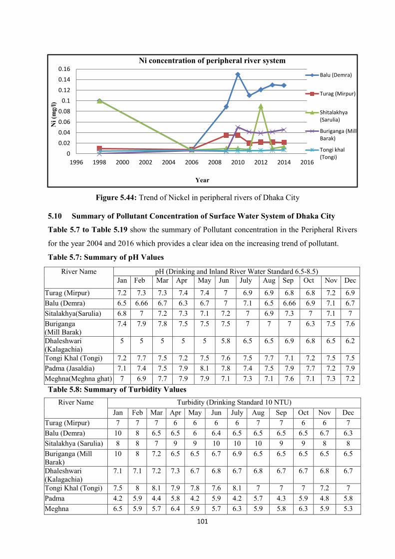
Figure 5.44 Trend of Nickel in peripheral rivers of Dhaka City .......................................... 102
Page 16
xiii
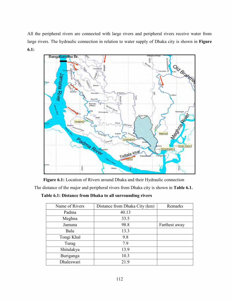
Figure 6.1 Location of Rivers around Dhaka and their Hydraulic connection ................... 112
Figure 6.2 Flow Hydrograph of Turag River.......................................................................... 113
Figure 6.3 Flow Hydrograph of Tongi khal......................... ......................... ........................ 114
Figure 6.4 Flow Hydrograph of Balu .. ......................... .................... ......................... ...... 114
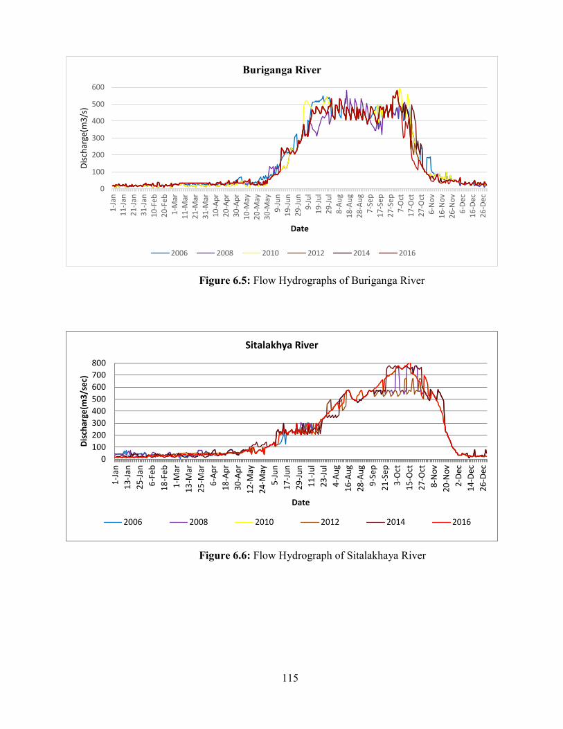
Figure 6.5 Flow Hydrograph of Buriganga .. ......................... ........................................... 115
Figure 6.6 Flow Hydrograph of Sitalakhaya ... ......................... ......................... ............... 115
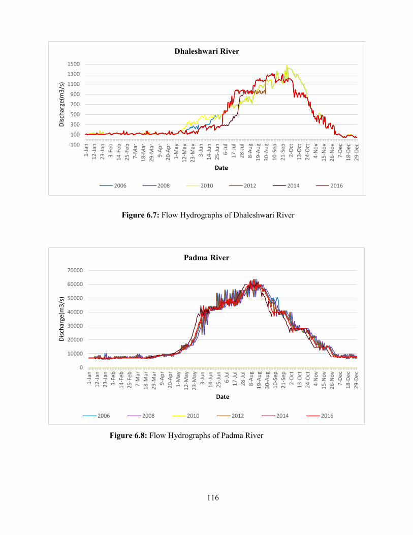
Figure 6.7 Flow Hydrograph of Dhalaeswari ... ......................... ........................................ 116
Figure 6.8 Flow Hydrograph of Padma .. ......................... ......................... ........................ 116
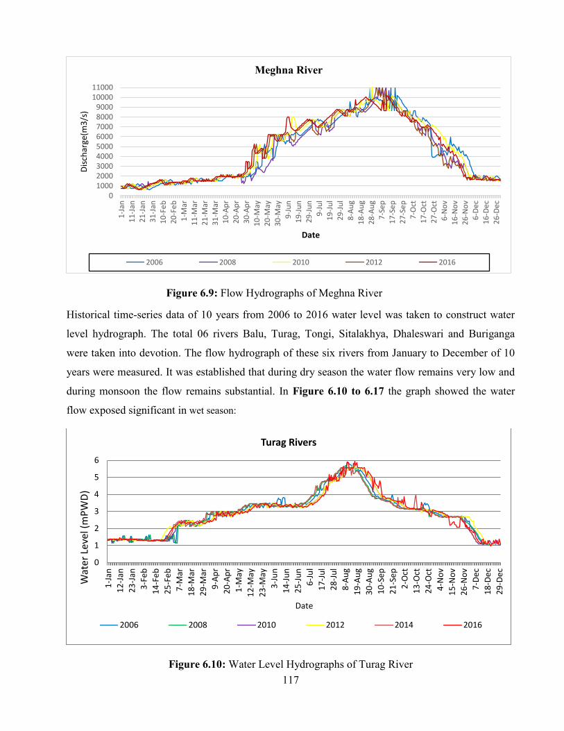
Figure 6.9 Flow Hydrograph of Meghna ... ......................... ......................... .................... 117
Figure 6.10 Water Level Hydrograph of Turag .. ......................... ......................... .............. 117
Figure 6.11 Water Level Hydrograph of Tongi Khal .. ......................... ............................. 118
Figure 6.12 Water Level Hydrograph of Balu ..... .................................... ........................... 118
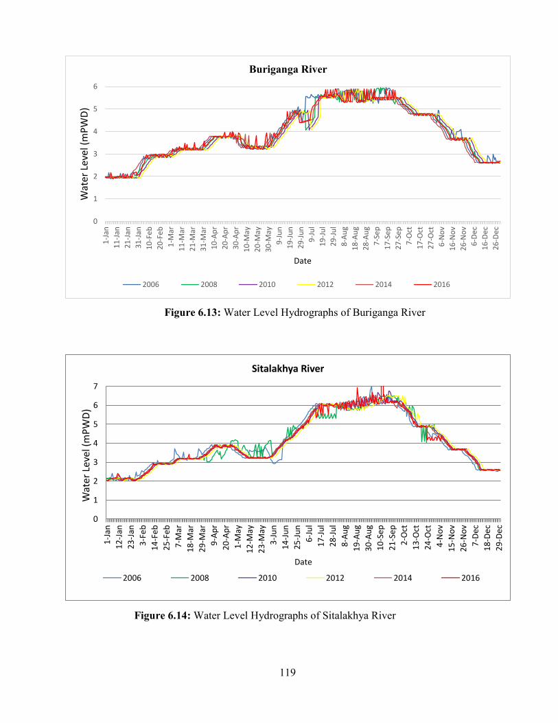
Figure 6.13 Water Level Hydrograph of Buriganga .. ......................... ......................... ...... 119
Figure 6.14 Water Level Hydrograph of Sitalakhya ... ......................... ........................... 119
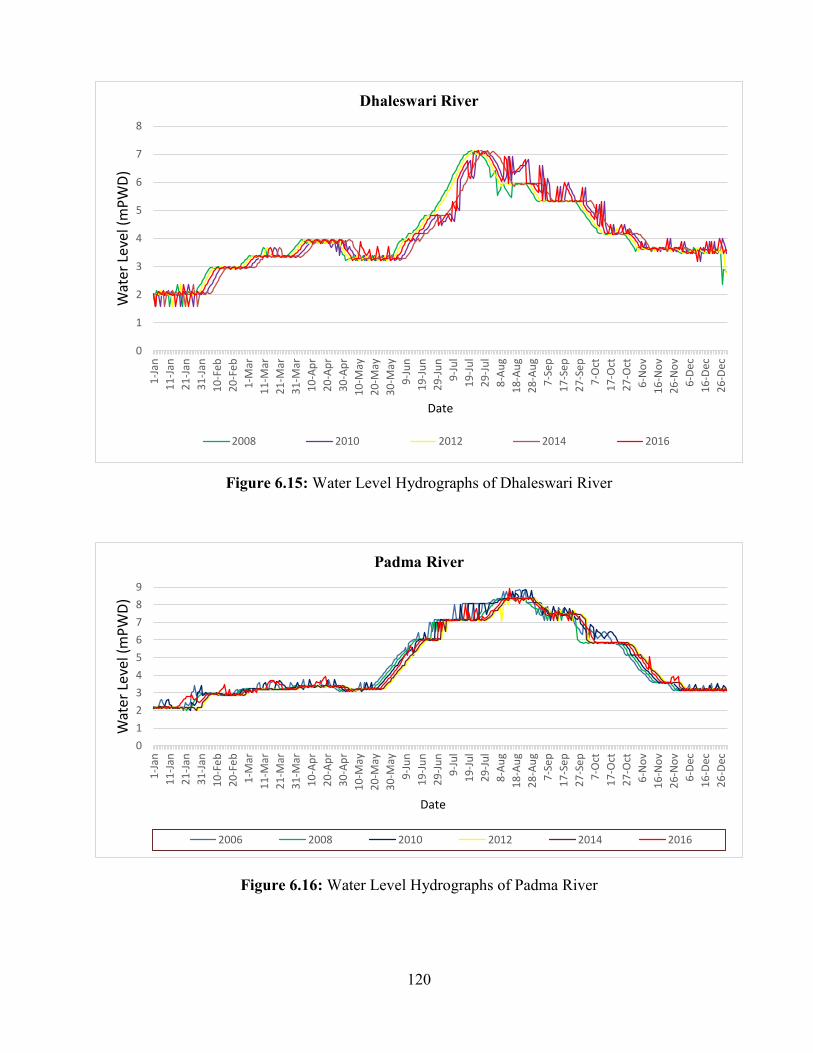
Figure 6.15 Water Level Hydrograph of Dhaleswari .. ......................... ............................. 120
Figure 6.16 Water Level Hydrograph of Padma .... ......................... .................................. 120
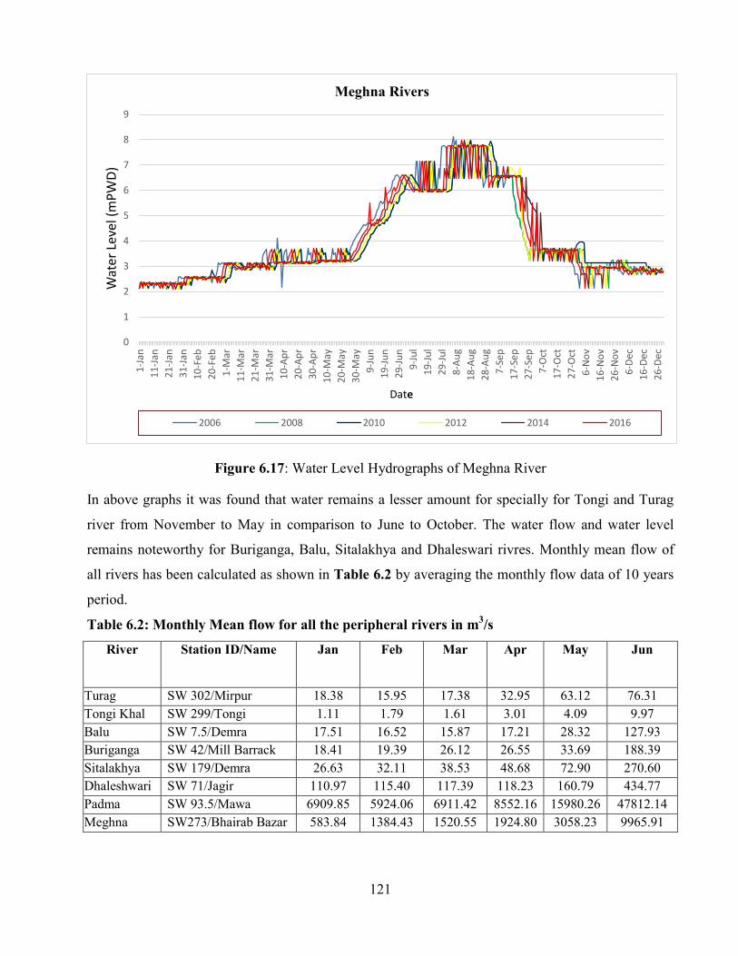
Figure 6.17 Water Level Hydrograph of Meghna ............................................................... 121
Figure 6.18 Flow Duration Curve of Turag River .............................................................. 123
Figure 6.19 Flow Duration Curve of Tongi River .............................................................. 124
Figure 6.20 Flow Duration Curve of Balu River ................................................................ 124
Figure 6.21 Flow Duration Curve of Buriganga River ....................................................... 125
Figure 6.22 Flow Duration Curve of Sitalakhya River ....................................................... 125
Figure 6.23 Flow Duration Curve of Daleshwari River ...................................................... 126
Figure 6.24 Flow Duration Curve of Padma River ............................................................. 126
Figure 6.25: Flow Duration Curve of Meghna River .. ......................... ................................... 127
Figure 6.26: Available Depths of Peripheral Rivers......... ......................... .......................... 130
Figure 6.27: HEC RAS Model Boundary Locations ................................................................. 135
Figure 6.28 Boundary discharge (Q) data of Balu river...................................................... 136
Figure 6.29 Boundary Discharge (Q) data of Lakhya River.................................................. 136
Figure 6.30 Boundary Discharge (Q) data of Turag River.................................................. 137
Figure 6.31 Boundary Discharge (Q) data of Dhaleswari River............................................... 137
Figure 6.32 Boundary Water level (WL) data of Dhaleswari River.................................. 138
Figure 6.33: Hydrodynamic model Set up of River network...................................................... 139
Page 17
xiv
Figure 6.34: Calibration of the numerical model of Turag River in Year 2014 ........................ 140
Figure 6.35: Validation of the numerical model of Turag River in Year 2015 ......................... 140
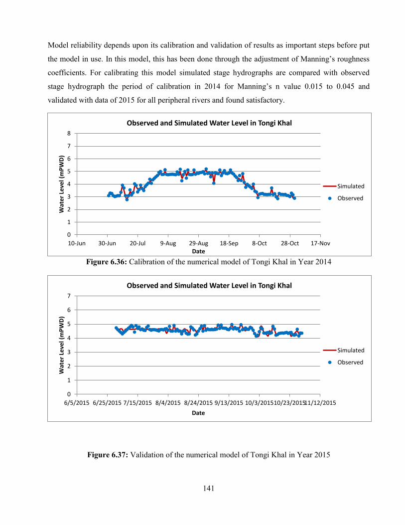
Figure 6.36: Calibration of the numerical model of Tongi Khal in Year 2014 ........................ 141
Figure 6.37: Validation of the numerical model of Tongi Khal in Year 2015 ......................... 141
Figure 6.38: Calibration of the numerical model of Balu River in Year 2014 ......................... 142
Figure 6.39: Validation of the numerical model of Balu River in Year 2015 .......................... 142
Figure 6.40: Calibration of the numerical model of Buriganga River in Year 2014 ................ 143
Figure 6.41: Validation of the numerical model of Buriganga River in Year 2015 ................. 143
Figure 6.42: Calibration of the numerical model of Sitalakhya River in Year 2014 ............... 144
Figure 6.43: Validation of the numerical model of Sitalakhya River in Year 2015 ............... 144
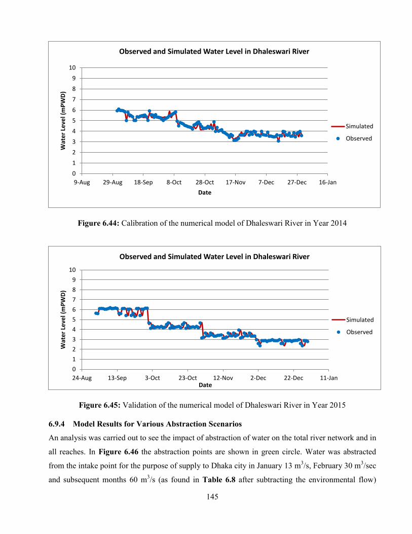
Figure 6.44: Calibration of the numerical model of Dhaleswari River in Year 2014 .............. 145
Figure 6.45: Validation of the numerical model of Dhaleswari River in Year 2015 ............... 145
Figure 6.46: Map showing the abstraction points in the river network......................................... 147
Figure 6.47: Variation of Velocity Before and After Abstraction along the Turag River ......... 149
Figure 6.48: Variation of Water Level Before and After Abstraction along the Turag River ... 149
Figure 6.49: Variation of Water Depth Before and After Abstraction along the Turag River... 150
Figure 6.50: Variation of Velocity Before and After Abstraction along the Tongi River .... ..... 150
Figure 6.51: Variation of Water Level Before and After Abstraction along the Tongi Khal .... 151
Figure 6.52: Variation of Water Depth Before and After Abstraction along the Tongi Khal .... 151
Figure 6.53: Variation of Velocity Before and After Abstraction along the Balu River ........... 152
Figure 6.54: Variation of Water Level Before and After Abstraction along the Balu River ..... 153
Figure 6.55: Variation of Water Depth Before and After Abstraction along the Balu River .... 153
Figure 6.56: Variation of Velocity Before and After Abstraction along the Buriganga River .. 154
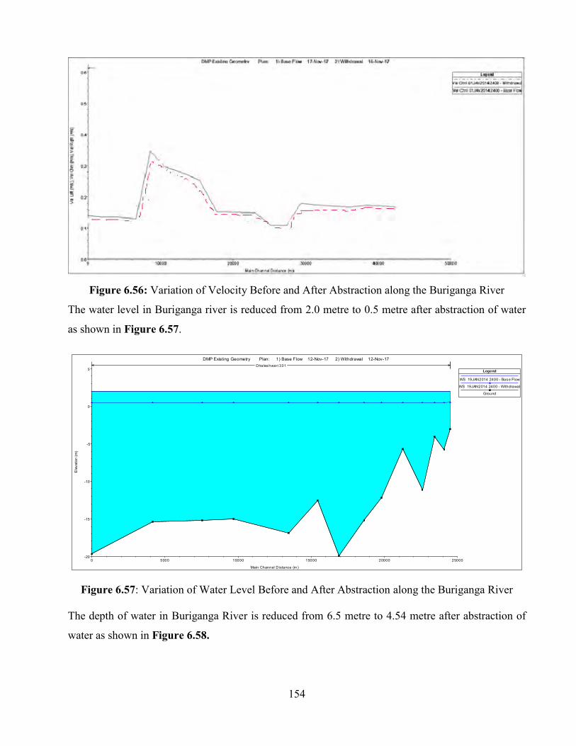
Figure 6.57: Variation of Water Level Before and After Abstraction along the Buriganga River. 154
Figure 6.58: Variation of Water Depth Before and After Abstraction along the Buriganga River.. 155
Figure 6.59: Variation of Velocity Before and After Abstraction along the Shitalakya River ....... 155
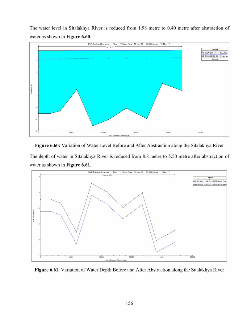
Figure 6.60: Variation of Water Level Before and After Abstraction along the Sitalakhya River . 156
Figure 6.61: Variation of Water Depth Before and After Abstraction along the Sitalakhya River . 156
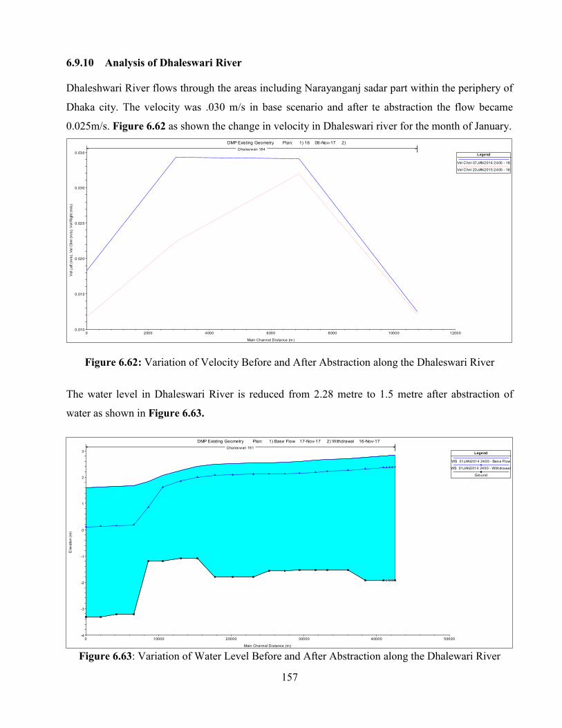
Figure 6.62: Variation of Velocity Before and After Abstraction along the Dhaleswari River .... 157
Figure 6.63 Variation of Water Level Before and After Abstraction along the Dhalewari River .. 157
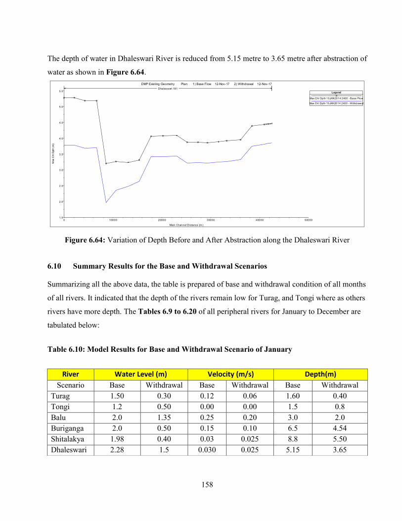
Figure 6.64 Variation of Water Depth Before and After Abstraction along the Dhaleswari River .158
Figure 7.1 Prediction of demand components of Dhaka city................................................ 160
Figure 7.2 Net Water Availability of Balu River ……………….………….………….… 167
Page 18
xv
Figure 7.3 Net Water Availability of Turag River …………….………….………….… 167
Figure 7.4 Net Water Availability of Tongi River………………….………….………….… 168
Figure 7.5 Net Water Availability of Buriganga River ………….………….………….… 168
Figure 7.6 Net Water Availability of Sitallakhya River ………….………….………….… 169
Figure 7.7 Net Water Availability of Dhaleswari River ……….………….………….… 169
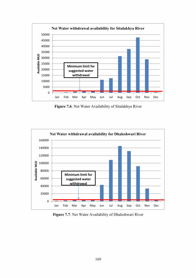
Figure 7.8 Net Water Availability of Padma River ……….………….………………… 170
Figure 7.9 Net Water Availability of Meghna River ………….………….……………… 170
Figure 7.10 Important Water Quality Parameters of Peripheral Rivers …………………. 172
Figure 7.11 Comparisons of Water Quality Parameters between Two Large Rivers (Padma
and Meghna) and One of the Peripheral Rivers (Buriganaga) ……………………………… 172
Figure 7.12 Water availability and Quality.. …………………………………………… .. 176
Figure 7.13 Water Availability and Cost Effectiveness…………………………………. 177
Figure 7.14 Shift towards surface water from ground water …………………...……….. 180
Page 19
xvi
LIST OF TABLES
Table 1.1 Study Area Coverage ………………………………………………………. 8
Table 1.2 Summary of Peripheral Rivers ……………………………………….. 10
Table 2.1 Important Water Quality Standards ……………………………………….. 16
Table 2.2 Water Supply Scenario in different cities …………………………..……… 27
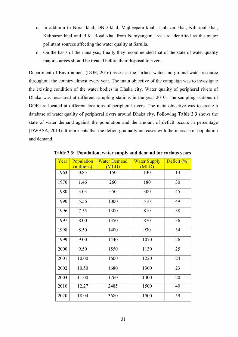
Table 2.3 Population, water supply and demand for various ……..……..……..……… 30
Table 2.4 Priority of Evaluating of Additional Measures…………………………….…. 42
Table 3.1 Water quality monitoring station of DOE ………………………………… 47
Table 3.2 Water quality monitoring station of DWASA (2014 -2016)……………… 48
Table 3.3 Bathymetry Data ………………………………………………………… 50
Table 3.4 Water Level and Discharge Stations …………………………………… 51
Table 3.5 Summary of the activities …………………………………………… 56
Table 4.1 Groundwater Depletion State in Lalbag, Motijheel, Cantonment, Mirpur,
Tejgoan and Dhanmondi................................................................................ 58
Table 4.2 Details of SWTPs.......................................................................................... 60
Table 4.3 Population Projection …………………...………….................................... 62
Table 4.4 Breakdown of indoor household water consumption from field survey....... 63
Table 4.5 Estimation of projected water demand from 2017 upto 2035...... ....... 65
Table 4.6 Estimation of projected water demand from 2040 upto 2060...... ....... 65
Table 5.1 Locations for the analysis of water quality parameters of Padma River) …. 69
Table 5.2(a) Summary characteristics of surface water samples collected in July 2009... . 75
Table 5.2(b) Summary characteristics of surface water samples collected in November 2009 75
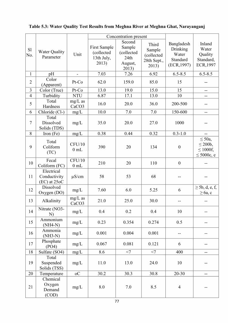
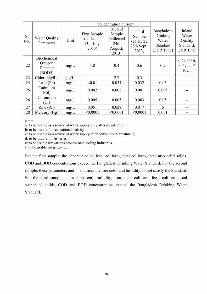
Table 5.3 Water Quality Test Results from Meghna River at Meghna Ghat, Narayanganj 77
Table 5.4 Four water quality parameters of Balu River ................................................. 80
Table 5.5 DO Sample of Balu River for a stretch of 42 km ........................................... 81
Table 5.6 Locations for the analysis of water quality parameters of Buriganga River ... 91
Page 20
xvii
Table 5.7 Summary of pH Parameter ............................................................................... 102
Table 5.8 Summary of Turbidity Parameter ..................................................................... 102
Table 5.9 Summary of Chloride Parameter ..................................................................... 103
Table 5.10 Summary of NH4 Parameter ........................................................................... 103
Table 5.11 Summary of DO Parameter .............................................................................. 103
Table 5.12 Summary of BOD Parameter .......................................................................... 104
Table 5.13 Summary of TDS Parameter ........................................................................... 104
Table 5.14 Summary of Lead (Pb) Parameter .................................................................. 104
Table 5.15 Summary of Cadmium (Cd) Pollution Parameter .......................................... 105
Table 5.16 Summary of Chromium (Cr) Pollution Parameter .......................................... 105
Table 5.17 Summary of Zinc (Zn) Pollution Parameter ................................................... 105
Table 5.18 Summary of Mercury (Hg) Pollution Parameter ............................................ 106
Table 5.19 Summary of Phosphate (PO4) Pollution Parameter ...................................... 106
Table 5.20 Summary of Pollutant Loading in the Peripheral Rivers ................................... 107
Table 5.21 Important Flow Characteristics of Padma River ………………………….... 107
Table 5.22 Important Value of Padma River ………………........................................... 108
Table 6.1 Distance from Dhaka to All Surrounding Rivers ..................................……. 112
Table 6.2 Monthly Mean flow for all the peripheral rivers in m3/s ............................... 121
Table 6.3 Environmental Flow Requirement using 10% MAF Method ........................... 123
Table 6.4 Flow Q90 and Q50 for the selected rivers................................................................ 127
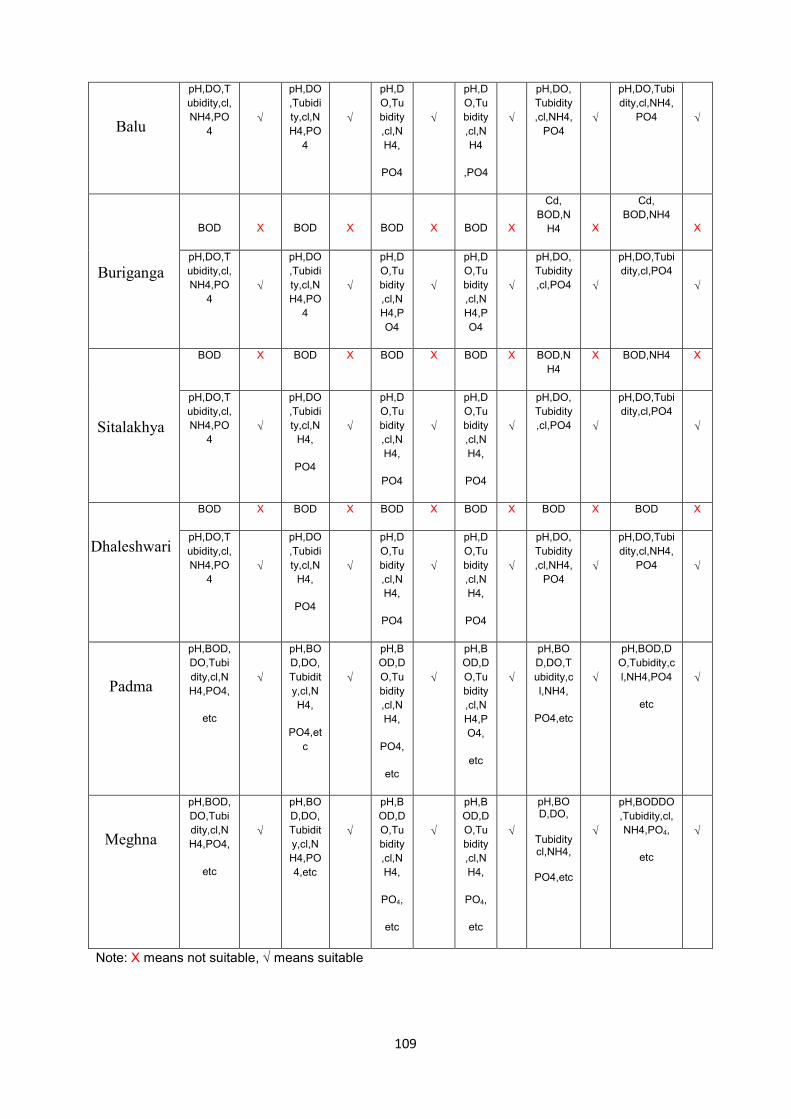
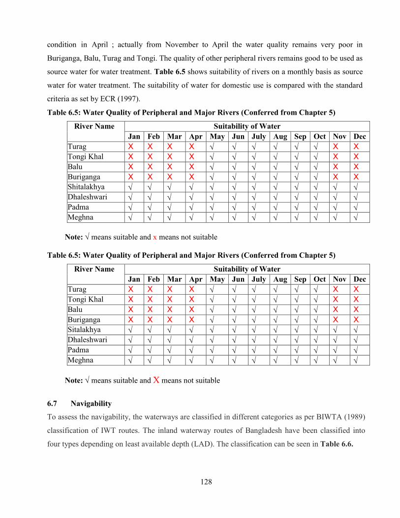
Table 6.5 Water Quality of Peripheral and Major Rivers (Conferred from Chapter 5) . 128
Table 6.6 Classification of IWT Route according to BIWTA .......................................... 128
Table 6.7 Available Depths, Water level and Navigability of Peripheral Rivers.................. 129
Table 6.8 Availability of Surface Water ........................................................................... 131
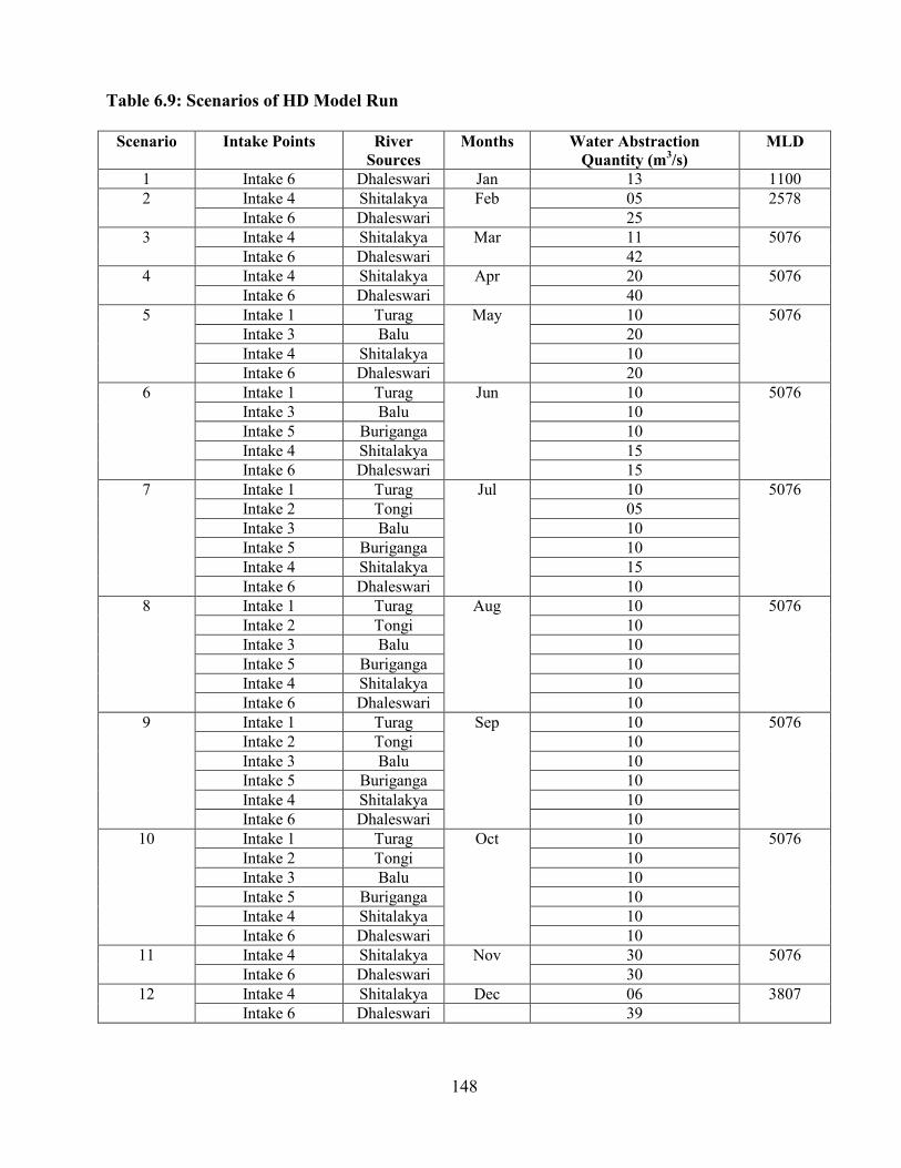
Table 6.9 Scenarios of HD Model Run............................................................................ 148
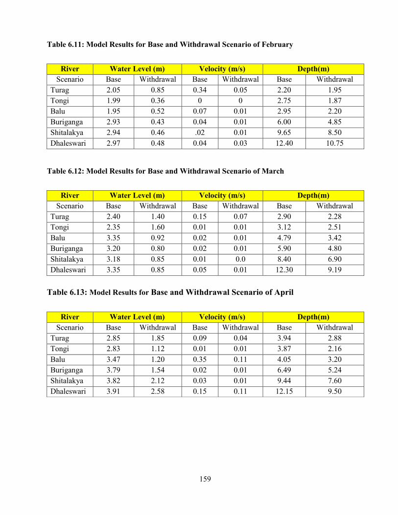
Table 6.10 Model Results for Base and Withdrawal Scenario of January............................. 158
Table 6.11 Model Results for Base and Withdrawal Scenario of February........................... 159
Table 6.12 Model Results for Base and Withdrawal Scenario of March............................... 159
Table6.13 Model Results for Base and Withdrawal Scenario of April ............................... 159
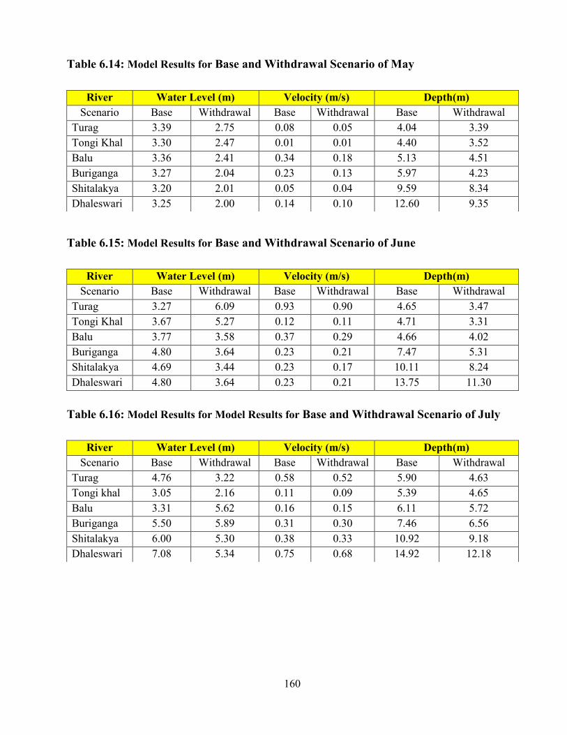
Table 6.14 Model Results for Base and Withdrawal Scenario of May ............................... 160
Table6.15 Model Results for Base and Withdrawal Scenario of June................................. 160
Table 6.16 Model Results for Base and Withdrawal Scenario of Jul .................................. 160
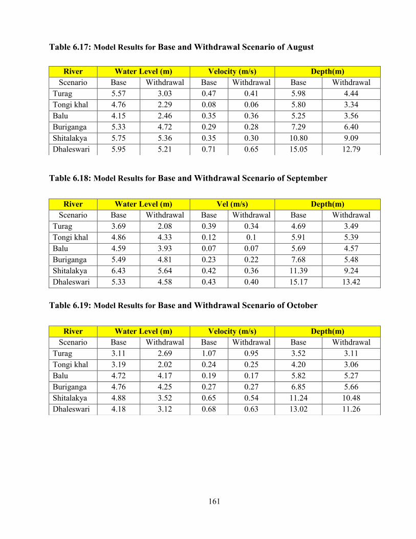
Table 6.17 Model Results for Base and Withdrawal Scenario of Aug ................................ 161
Page 21
xviii
Table 6.18 Model Results for Base and Withdrawal Scenario of Sep........................................ 161
Table 6.19 Model Results for Base and Withdrawal Scenario of Oct................................. 161
Table 6.20 Model Results for Base and Withdrawal Scenario of Nov ...................................... 162
Table 6.21 Model Results for Base and Withdrawal Scenario of Dec .................................... 162
Table 7.1 Water Availability Index ……………………………………………………… 171
Table 7.2 Dry Period Water Quality Index ........................................................................ 173
Table 7.3 Total Water Treatment Plant (WTP) Cost ....………………………………... 173
Table 7.4 Operational Expenditure ……………………………………………………… 174
Table 7.5 Cost per MLD ............................................................................................... 175
Table 7.6 Cost Effectiveness ……………………………………………………………. 175
Table 7.7 Overall Index of all the Rivers ……………………………………………….. 176
Table 7.8 Estimated Water Availability from Peripheral Rivers ………………………… 178
Table 7.9 Ongoing Water Utilization Plan of Large Rivers …………………………… 178
Table 7.10 Suggested Plan for Future Water Production ...................................................... 179
Table 7.11 Year-wise Financial Requirement (Crore Taka) ……………………………. 180
Page 22
xix
LIST OF ABBREVIATIONS
Abbreviation Meaning
BBS
Bangladesh Bureau of Statistics
BGMEA Bangladesh Garment Manufacturers and Exporters Association
BOD Biochemical Oxygen Demand
BUET Bangladesh University of Engineering and Technology
BWDB Bangladesh Water Development Board
cumec Cubic Meter per Second
DOE Department of Environment
DOH Department of Hydrology
DTW Deep Tube Well
DWASA Dhaka Water Supply and Sewerage Authority
EPB Export Promotion Bureau
FGD Focus Group Discussion
GIS Global Information System
gpcd Gallon per Capita per Day
IDI In-depth Interview
IWM Institute of Water Modeling
KII Key Informant Interview
km Kilometer
LIC Low Income Community
lpcd Liter per Capita per Day
MIST Military Institute of Science and Technology
MLD Million Liter per Day
NSU North South University
Page 23
xx
NTU Nephelometric Turbidity Units
Pt-Co Platinum-Cobalt
SPSS Statistical Package for the Social Sciences
SWTP Surface Water Treatment Plant
WARPO Water Resource Planning Organization
WHO World Health Organization
Page 24
1
CHAPTER ONE
INTRODUCTION
1.1 General
Water constitutes two-thirds of the surface of the earth. Water is an indispensable constituent of all
organisms and usually a good solvent for a large variety of ingredients. Moreover, being necessary
for most biotic processes makes it one of the major modules of socio-economic development and
scarcity alleviation. Water resources have infinite importance in human survival, socio-economic
stability and environmental sustainability. Though water covers 71 percent of the earth's surface,
but only three percent is fresh water out of which 69 percent is "trapped" as ice, mainly in the two
Polar Regions. The remaining freshwater occurs in rivers, lakes and aquifers which human being,
plants and other animal species can use. The distribution must be carefully managed to avoid
irreversible depletion of the resource (WHO/UNICEF JMP, 2012). United Nations proclaimed that
the water act as a dynamic force for a continued development and a strategic tool to fight against
poverty as per concept of sustainable development goals. 2.6 billion people have gained access to
improved drinking water sources since 1990, but 663 million people are still without safe water.
Ensure access to water and sanitation for all is the main concept of United Nations Sustainable
Development Goals (http/www.un.org). Moreover, this study also focuses implementation towards
Sustainable Development Goal (SDG- 6) prescribed by United Nations in 2016.
Water scarcity has been triggering conflict since a long time due to many tangible and intanib
factors. Kjellén and McGranahan (1997) predicted that two-thirds of the world’s population will
experience water stress condition by 2025. Many countries will experience high water stress
condition where available water resources withdrawal exceeds the limit. Statistics showed that one
in eight people does not have access to safe drinking water and two of five people do not have
adequate sanitation worldwide (Water Aid, 2010). Life cannot sustain without water. Moreover,
lack of access to adequate safe water leads to the spreading of diseases. Children and women bear
the greatest health burden associated with unsafe water and sanitation. World Health Organization
(2012) estimated that 1.73 million deaths occur each year due to diarrheal diseases attributed from
poor water supply, sanitation and hygiene. This situation becomes more problematic in South Asia,
where withdrawal rate against available resources is 48 percent (Ariyabandu, 1999).
Page 25
2
Bangladesh being a riverine country has been facing many fold challenges from safe drinking
water, say for example, unlimited flood water during wet season, increasing scarcity during dry
season and management of all resources under serious threat. Water experiences socio-ecological
resource management at which decisions are made for water scheming does not match with its
requirement. The urban water management requires a systematic process that includes planning,
research, design, engineering, regulation, and administration. Under this circumstance, the current
study has attempted to comprehend the present and future trend and extent of water demand and
supply. This study will be carried out through analyzing status of surface and groundwater and
options for surface water availability sources based upon future demand and supply projection.
Particular attention has been given to elucidate the quantity, quality and cost effectiveness to
achieve safe water to meet the future demand of Dhaka city.
A rapid increase in the pace of rural-urban migration has been very explicit in the recent decades in
Bangladesh. The urbanization coupled with pressure from fast-rising population has been exposing
the city authorities to a growing demand for increased quality and quantum of urban-specific
services. Now challenges due to rapid urbanization are multidimensional. Dhaka city has been
increasing in its volume with an annual rate of 3.5 percent following an unsystematic approach
(Islam et al., 2009) to accommodate huge population influx of more than seven million (BBS,
2009) people. Such urban sprawl exerts immense pressure on the infrastructures of the city. The
city inhabitants, therefore, are deprived of basic amenities of urban life where water supply has
appeared as the most critical issue. At present, water demand has surpassed the water supply where
25 percent of the total population of Dhaka city has no direct access to potable water (Nishat, et
al., 2008). Dhaka Water Supply and Sewerage Authority (DWASA) is the stakeholder and
responsible for water supply throughout the city, which has revised their area of responsibility over
the years. Dhaka Statistical Metropolitan Area (DSMA) covers an area of 1353 km2, out of which
Dhaka Metropolitan Area (DMA) constitutes 27 percent (360 km2). Until 1989, Dhaka Water
Supply and Sewerage Authority (DWASA) operation was limited to DMA. In 1990 DWASA
extended operating area to adjacent Narayangonj metropolitan area. In recent times, Dhaka city is
facing more difficulties in maintaining adequate water supply mainly due to following reasons:
a. Rapidly growing population and demand
b. Declining of ground water level
c. Inadequate surface water to cope with the future demand
d. Poor raw water quality
Page 26
3
e. Leakages in the system network
f. Existing inadequate pipe network design
In addition, the city water supply system is also facing challenges due to unplanned city
development and informal settlements, switching to surface water instead of groundwater and
requirement of large financial investment. However, Dhaka city water supply system has also
number of achievements. The main achievements are increase of water production, improved
service quality, reduction of non-revenue water and provision of water supply at low cost.
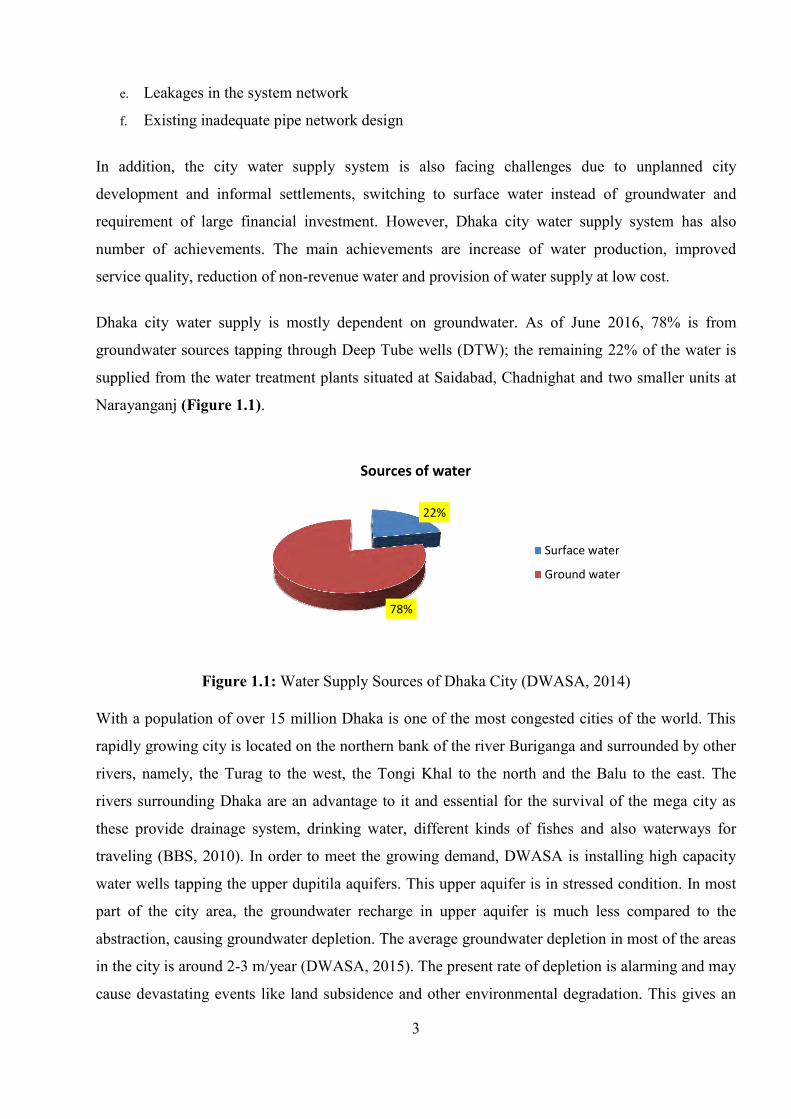
Dhaka city water supply is mostly dependent on groundwater. As of June 2016, 78% is from
groundwater sources tapping through Deep Tube wells (DTW); the remaining 22% of the water is
supplied from the water treatment plants situated at Saidabad, Chadnighat and two smaller units at
Narayanganj (Figure 1.1).
Figure 1.1: Water Supply Sources of Dhaka City (DWASA, 2014)
With a population of over 15 million Dhaka is one of the most congested cities of the world. This
rapidly growing city is located on the northern bank of the river Buriganga and surrounded by other
rivers, namely, the Turag to the west, the Tongi Khal to the north and the Balu to the east. The
rivers surrounding Dhaka are an advantage to it and essential for the survival of the mega city as
these provide drainage system, drinking water, different kinds of fishes and also waterways for
traveling (BBS, 2010). In order to meet the growing demand, DWASA is installing high capacity
water wells tapping the upper dupitila aquifers. This upper aquifer is in stressed condition. In most
part of the city area, the groundwater recharge in upper aquifer is much less compared to the
abstraction, causing groundwater depletion. The average groundwater depletion in most of the areas
in the city is around 2-3 m/year (DWASA, 2015). The present rate of depletion is alarming and may
cause devastating events like land subsidence and other environmental degradation. This gives an
22%
78%
Sources of water
Surface water
Ground water
Page 27
4
alarming indication that there is an urgent need to alleviate pressure on the upper aquifer being
exploited and explore for more suitable and sustainable sources to supplement the present water
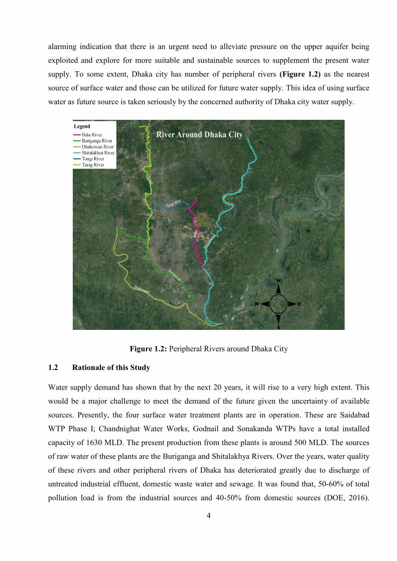
supply. To some extent, Dhaka city has number of peripheral rivers (Figure 1.2) as the nearest
source of surface water and those can be utilized for future water supply. This idea of using surface
water as future source is taken seriously by the concerned authority of Dhaka city water supply.
Figure 1.2: Peripheral Rivers around Dhaka City
1.2 Rationale of this Study Water supply demand has shown that by the next 20 years, it will rise to a very high extent. This
would be a major challenge to meet the demand of the future given the uncertainty of available
sources. Presently, the four surface water treatment plants are in operation. These are Saidabad
WTP Phase I; Chandnighat Water Works, Godnail and Sonakanda WTPs have a total installed
capacity of 1630 MLD. The present production from these plants is around 500 MLD. The sources
of raw water of these plants are the Buriganga and Shitalakhya Rivers. Over the years, water quality
of these rivers and other peripheral rivers of Dhaka has deteriorated greatly due to discharge of
untreated industrial effluent, domestic waste water and sewage. It was found that, 50-60% of total
pollution load is from the industrial sources and 40-50% from domestic sources (DOE, 2016).
Page 28
5
Although there is sufficient water in the peripheral rivers, but because of large scale pollution, the
water of the peripheral rivers is no longer considered viable for a treatment plant in the long run.
The Narayanganj WTPs (Godnail and Sonakanda) is planned to be expanded and rehabilitated to
produce more water in coming years.This scenario is considered to be realistic, yet conservative as
it assumes an increase in per capita consumption after rehabilitation of the network and a constant
(and relatively high) per capita demand hereafter.
Dhaka city is experiencing groundwater recharge deficit every year. Moreover, increased rate of
urbanization, illegal occupation, and encroachment reduce the amount and volume of surface water
bodies around the city that deteriorate the present situation.
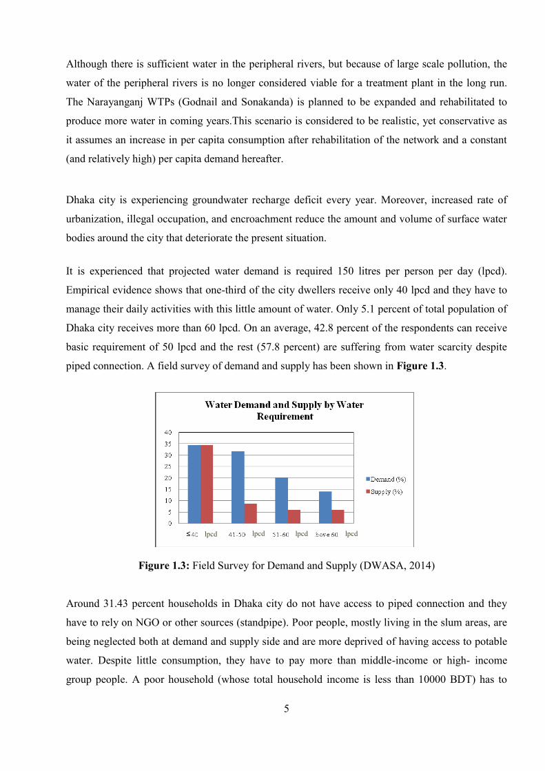
It is experienced that projected water demand is required 150 litres per person per day (lpcd).
Empirical evidence shows that one-third of the city dwellers receive only 40 lpcd and they have to
manage their daily activities with this little amount of water. Only 5.1 percent of total population of
Dhaka city receives more than 60 lpcd. On an average, 42.8 percent of the respondents can receive
basic requirement of 50 lpcd and the rest (57.8 percent) are suffering from water scarcity despite
piped connection. A field survey of demand and supply has been shown in Figure 1.3.
Figure 1.3: Field Survey for Demand and Supply (DWASA, 2014)
Around 31.43 percent households in Dhaka city do not have access to piped connection and they
have to rely on NGO or other sources (standpipe). Poor people, mostly living in the slum areas, are
being neglected both at demand and supply side and are more deprived of having access to potable
water. Despite little consumption, they have to pay more than middle-income or high- income
group people. A poor household (whose total household income is less than 10000 BDT) has to
≤ lpcd lpcd lpcd lpcd
Page 29
6
spend 500 BDT per month for 30 lpcd while a middle-income or high-income group family (whose
total household income is more than 10000 BDT) has to pay 400 BDT/month for water supply of
45-50 lpcd or more. Poor people have to buy additional water to maintain their daily activities. This
extra spending of water hinders to improve the livelihood status. Despite dominance of
uncontaminated groundwater in DWASA water supply system, the user-end water quality exceeds
World Health Organization’s (WHO) prescribed drinking water permissible limit due to poor
maintenance. A study found that about 22.86 percent city dwellers could not use the DWASA
supply for drinking purpose due to bad smell and have to rely on bottled or jar water that is of
dubious quality. On the other hand, 66 percent of the consumers boil DWASA supplied water for
drinking purpose and they have to boil the water at least for half an hour to make it potable. Among
them, at least 50 percent also use water filter to ensure maximum safety (DWASA, 2015). Two-
thirds of the Dhaka city dwellers believe that current water supply management system could not
fulfill their demand. The present study has attempted to focus few scenarios considering existing
water supply situation, future demand, water availability, water quality and finally cost
effectiveness of surface water sources of Dhaka City up to 2035. It is apprehended that all of these
scenarios showed a mismatch between water demand and supply.
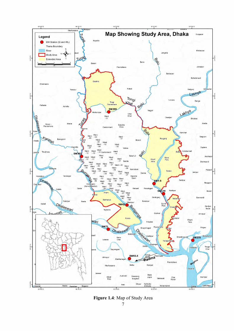
1.3 Study Area
The study area encompasses area of present Dhaka city and planned future extension. The area is
located within 90°47′ N latitude to 90°18′ E longitude. There are six rivers flowing along its
periphery, notable of which are Buriganga, Shitalakhya, Balu, Dhaleshwari, Turag and Tongikhal.
The study area covers about 617 km2 of Dhaka city as shown in Figure 1.4.
Page 30
7
Figure 1.4: Map of Study Area
Page 31
8
The existing Dhaka city service area covers approximately 497 km2 and includes some localities
that are not mentioned in DWASA 1996 Act (parts Bandar Thana). The service area would expand
to cover not only all of the existing jurisdiction area but also some neighboring locations in
Madanpur and Dhamghar area. The study area is approximately 617 km2 covering following area as
per Table 1.1. Figure 1.4 shows the study area with future extension in yellow shaded area beyond
the red boundary
Table 1.1: Study area coverage
Serial Region Area Coverage (km2)
1. Main Dhaka City 303
2. Tongi and Gachcha 61
3 Rupganj(Purbachal) 97
4. Bandar 36
5. Keraniganj and Kalagachia Approx. 120
Total 617
1.4 Brief Description of the Peripheral Rivers System Dhaka City is surrounded by rivers in its periphery as shown in Figure 1.2. Buriganga, Turag, Balu,
Shitalakhya, Dhaleswari and Tongi Khal engulf the City. The river Buriganga takes name as
Buriganga from the end of Turag at Ameen bazar union of Savar upazilla, flows through the
southern part of Dhaka city and meets Dhaleshwari River at Konda union of Keraniganj upazilla.
The main flow of the Buriganga comes from the Turag only. The present head of the Buriganga
near Chaglakandi has silted up and opens only during flood, but the lower part is still open
throughout the year. Water pollution in the River Buriganga is at its highest. The most significant
source of pollution appears to be from tanneries in the Hazaribagh area. In the dry season, the
dissolved oxygen level becomes very low or non-existent and the river becomes toxic (Quader S,
2015). Shitalakhya River having a length of 113 km flows through Monohordi Upazilla of
Norshingdi district and then east of the city of Narayanganj in central Bangladesh until it merges
with the Dhaleswari near Kalagachhiya. The river joins the river Balu at Demra, a small tributary
flowing from the north of greater Dhaka. About 20 km downstream of Demra, the Sitalakhya River
joins the Dhaleswari River at the Bandar upazilla of Narayanganj district (BWDB, 2010). There are
several different types of industries like textiles and dyeing, paper and pulp, jute, pharmaceuticals,
fertilizers, etc of moderate to big size and several urban developments along the entire stretch of the
river (Alam et al, 2012). These establishments contributed to the pollution load to the Sitalakhya
River directly or through a number of wastewater canals like DND drainage canal Killarpul khal,
Page 32
9
Kalibazar khal, Tanbazar khal etc. Domestic and industrial wastewater from Dhaka city through
Norai khal and from the Tongi industrial area through Tongi khal disposed of in the river Balu. This
also contributed to the pollution load to the river Sitalakhya. The water quality of this river is of
particular importance for both the ecological and commercial reasons and for concerns regarding
safe drinking water supply to the city as the largest surface water treatment plant in Bangladesh
located at Saidabad draws water from it through the intake at Sarulia about 400 m downstream of
its confluence with the Balu river. Balu River, a tributary of the Shitalakhy a River runs mainly
through the extensive swamps of Beel Belai and those which are located at the east of Dhaka,
joining the Shitalakhya near Demra. It has a narrow connection with the Shitalakshya through the
Suti River near Kapasia and with the Turag River by way of the Tongi Khal. There is also a link
with the Shitalakhya near Kaliganj. Although it carries flood water from the Shitalakhya and the
Turag during the flood season, the Balu is of importance mainly for local drainage and access by
small boats (Quader S, 2015). Tejgaon metropolitan area is an industrial area which dispose about
12000 m3
untreated waste per day (Roy, 2013) consisting of residue of soap, dyeing,
pharmaceuticals, metals industries etc. Effluent of this industrial area is directly discharged into
Begunbari and Narai canal which carries the waste through Balu River and ultimately flows on
Sitalakhya River which is used in Saydabad water treatment plant for meeting water consumption
demand of Dhaka city dwellers. Thus Balu river and its canal system in Dhaka east especially Narai
canal is the most polluted area which is responsible for polluting Sitalakhya day by day and the
ultimate outcome of this pollution is Saydabad water treatment plant’s being in threat. Turag River
generates from Banshi River at Kaliakair and meets Buriganga at Kholamara of Keranjiganj. Turag
is a narrow and short river originating as a side channel from the river Bangshi near north-western
part of Gazipur and reaches Tongi. At Tongi, this channel divides into two, one flows eastward
direction as river Tongi khal and then Balu while the other towards westward direction as river
Turag. The river crosses Mirpur Bridge on Dhaka Aricha Highway at Amin Bazar and finally
merges into Buriganga (Khondkar et al 2013).The Dhaleshwari River with a length of 160
kilometres is a distributary of the Jamuna River in central part of Bangladesh. It starts off the
Jamuna near the northwestern tip of Tangail District. Dhaleshwari River divides into two parts after
running a short distance from its generation point of Jamuna. The part which flows south takes
name as Kaliganga and other which flows east takes name as Barinda, then it flows as Bangshi
River (south) up to Savar. Then the same river again flows as Dhaleshwari through the southern
part of greater Dhaka Zilla and finally the two flows merge to meet the Shitalakshya River near
Narayanganj District. This combined flow goes southwards to merge into the Meghna River. At
present a branch of Turag River, generating from the Birolia union of Savar Upazilla, flowing
Page 33
10
eastward side of Tongi and meeting Balu River at Trimohoni of Uttarkhanupazilla is known as
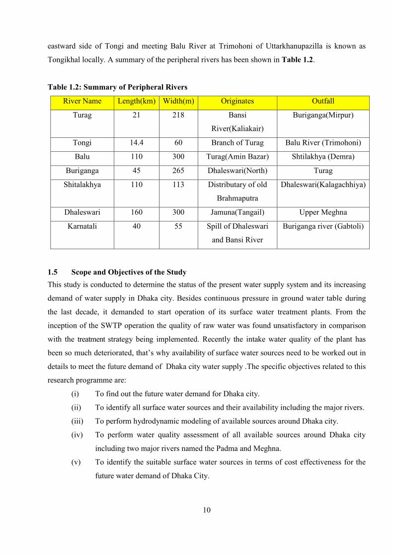
Tongikhal locally. A summary of the peripheral rivers has been shown in Table 1.2.
Table 1.2: Summary of Peripheral Rivers
River Name Length(km) Width(m) Originates Outfall
Turag 21 218 Bansi
River(Kaliakair)
Buriganga(Mirpur)
Tongi 14.4 60 Branch of Turag Balu River (Trimohoni)
Balu 110 300 Turag(Amin Bazar) Shtilakhya (Demra)
Buriganga 45 265 Dhaleswari(North) Turag
Shitalakhya 110 113 Distributary of old
Brahmaputra
Dhaleswari(Kalagachhiya)
Dhaleswari 160 300 Jamuna(Tangail) Upper Meghna
Karnatali 40 55 Spill of Dhaleswari
and Bansi River
Buriganga river (Gabtoli)
1.5 Scope and Objectives of the Study
This study is conducted to determine the status of the present water supply system and its increasing
demand of water supply in Dhaka city. Besides continuous pressure in ground water table during
the last decade, it demanded to start operation of its surface water treatment plants. From the
inception of the SWTP operation the quality of raw water was found unsatisfactory in comparison
with the treatment strategy being implemented. Recently the intake water quality of the plant has
been so much deteriorated, that’s why availability of surface water sources need to be worked out in
details to meet the future demand of Dhaka city water supply .The specific objectives related to this
research programme are:
(i) To find out the future water demand for Dhaka city.
(ii) To identify all surface water sources and their availability including the major rivers.
(iii) To perform hydrodynamic modeling of available sources around Dhaka city.
(iv) To perform water quality assessment of all available sources around Dhaka city
including two major rivers named the Padma and Meghna.
(v) To identify the suitable surface water sources in terms of cost effectiveness for the
future water demand of Dhaka City.
Page 34
11
1.6 Organization of the Report
The report is organized in eight chapters. In Chapter 1introduction of the thesis is outlined, in which
the study area, importance and objective of the study has been discussed. The review of the
literature is illustrated in Chapter 2 in which the previous study on water availability on ground
water and surface water sources has been reviewed. In Chapter 3 data collection and the
methodology of this study of water demand, quality, water availability and evaluation of surface
water sources of the study have been described. Chapter 4 will make an effort to analyze the future
population projection and future demand for the Dhaka city. In Chapter 5, water quality analysis of
surface water sources of Dhaka city has been illustrated. In Chapter 6, the analyses of availability of
surface water sources have been made. In Chapter 7, the evaluation of cost effectiveness aspects of
surface water sources has been described. Finally, conclusions and recommendations have been
summarized in Chapter 8.
Page 35
12
CHAPTER TWO
LITERATURE REVIEW
2.1 Introduction Dhaka is one of the most densely populated cities in the world, located in the central region of
Bangladesh. The city is surrounded mainly by the distributaries of Brahmaputra-Jamuna and
Meghna Rivers. These rivers are Buriganga, Dhaleswari, Balu, Turag, Tongi Khal and
Dhaleswari. Apart from these peripheral rivers there are two main rivers Padma and Meghna are
located adjacent to the capital city. The flow characteristics of the rivers are mainly controlled by the upstream flow. However, low
magnitude of tidal influence is observed at downstream of Balu and Buriganga River.
Hydrologically response of the rivers due to rapid urbanization, filling of low lands and
continuous population growth affecting the basin responses which, otherwise need to be assessed
carefully. Moreover, it is also important to assess the impacts of different potential scenarios and
different conditions. To meet the requirement of Dhaka city water demand, many analyses have
been carried out in different aspects by many researchers. Mostly all works have been carried out
related to ground water, surface water and water quality of peripheral rivers. Some of the review
of earlier works is shortly explained in subsequent paragraphs.
2.2 Description of Water Quality Parameters
Water quality in the rivers and water bodies are affected by point and non-point pollution sources.
However, the amounts and types of pollutants are not same from each source. As such,
contribution of pollutants from both sources should be assessed for effective water quality
management in river system. The point sources are outfall of pollutants from domestic, industrial
and commercial areas. In the case of non-point pollution sources the whole study area contributes
pollutants during flood events and rainfall runoff as per the land use and other conditions. To
assess the present condition of water quality, sampling has been taken from different points of the
river system. The primary objective of water quality monitoring is to obtain required information
for decision making and management and obtaining useful information depends on correct
interpretations of the measured variables in any water quality investigations. Water quality
variables, river or stream hydraulics, and the aquatic living organisms are all interrelated and
therefore interpreting the measured variables properly is vital for successful water quality
Page 36
13
monitoring plan. In following sections description of some important water quality parameters
have been briefly discussed.
Temperature of the water varies throughout the year and even throughout the day, but it will not
vary as much as the air temperature. This is important to aquatic lives, because they are very
sensitive to temperature changes. Temperature also affects aquatic life's sensitivity to toxic
wastes, parasites, and disease, either due to stress of rising water temperatures or the resulting
decrease in dissolved oxygen. Temperature and dissolved oxygen are closely related; the warmer
the water, the lesser the dissolved oxygen.
Turbidity is one of the important quality parameter. Any substance that makes water cloudy will
cause turbidity. The ability of light to pass through water depends on how much suspended
material is present. The most frequent causes of turbidity in rivers are soil erosion from mining,
dredging operations, and plankton. Erosion is a natural process which man speeds up by the use
of unsound farming practices, by logging forest areas in an uncontrolled way, by failing to
confine sediment runoff on construction sites. Rainfall causes a temporary increase in turbidity,
although this is a very common condition in Bangladesh with specific rainy seasons. Turbidity
affects fish and aquatic life by interfering with the penetration of sunlight. Water plants need light
for photosynthesis. If suspended particles block out light, photosynthesis and the production of
oxygen for fish and aquatic life will be reduced. If light levels get too low, photosynthesis may
stop altogether and algae will die. It is important to realize conditions of photosynthesis in plants,
increase respiration, oxygen use and the amount of carbon dioxide produced. Vegetation growth
in the water will be limited due to the reduced penetration of the light. Large amounts of
suspended matter may clog the gills of fish and shell fish and kill them directly. Turbid water
absorbs more sunshine, raising the temperature of the water and lowering the amount of dissolved
oxygen available for fish and aquatic life. Perhaps the most widespread problem throughout the
world is sedimentation. From above description, it is apparent that the turbidity test should be
done to know the quality of water.
Alkalinity is the water's ability to react with acids and neutralize their affect. Alkalinity protects
aquatic life by buffering the pH of the stream to a tolerable level. Total Alkalinity of range 100 -
200 mg/l will stabilize the pH level in a stream. However, alkalinity values between 20 and 200
are usually found in natural stream.
pH is one of the most common water quality tests to be performed. pH indicates the sample's
acidity, but is actually a measurement of the potential activity of hydrogen ions (H+) in the
samples. pH measurements run on a scale from 0 to 14, with pH value 7 considered as neutral.
Page 37
14
Solutions with a pH below 7 are considered acids. Solutions with a pH above 7, up to 14 are
considered bases. All organisms are subject to the amount of acidity of stream water and function
best within a given range. The pH of a body of water is affected by several factors. One of the
most important factors is the bedrock and soil composition through which the water moves both
in its bed and as groundwater. Some rock types such as limestone can, to an extent, neutralize the
acid while others, such as granite, have virtually no effect on pH. Another factor, which affects
the pH, is the amount of plant growth and organic material within a body of water. When this
material decomposes carbon dioxide is released. The carbon dioxide combines with water to form
carbonic acid. Although this is a weak acid, large amounts of it will lower the pH. This type of
effect is often seen in eutrophicated waters and can, together with the variation in the daily
oxygen content harm the fish population.
Organic pollution occurs when large quantities of organic matter reach a watercourse from
sources such as sewage, agricultural sources, urban run-off and industrial effluents such as waste
from food processing. The pollutants are a mixture of carbohydrates, fats and proteins and as such
are easily digestible by the micro-organisms that naturally reside in the receiving water body. The
bacteria reduce the amount of available oxygen in the water particularly in slow moving water. If
the lack of oxygen in water is severe may kill the fish and other aquatic life. The effects on biota
of organic pollution come from deoxygenation, toxicity and siltation acting either individually or
in combination.
Phosphates enter waterways from human and animal waste, phosphorus rich bedrock, laundry,
cleaning, industrial effluents, and fertilizer runoff. These phosphates become detrimental when
they over fertilize aquatic plants and cause eutrophication. This process results from the increase
of nutrients within the body of water which, in turn, create plant growth. Cultural eutrophication
is an unnatural speeding up of this process because of man's addition of phosphates, nitrogen, and
sediment to the water. Monitors should be aware that there are different kinds of phosphates in the
water, but a total phosphate-phosphorous reading is all that is needed to calculate the water
quality. If too much phosphate is present in the water the algae and weeds will grow rapidly and
may choke the waterway. Further, the rapid production of plant material will lead to a large
increase in oxygen levels in the daytime and a steep drop in the oxygen level during the night,
when the plants turn from oxygen production to respiration.
Nitrate in the water comes primarily from fertilizer runoff, leaky drains, and sewage discharges.
In nature, they generally are formed by the action of bacteria on ammonia and on compounds,
which contain nitrogen. Nitrite is a relatively short-lived form of nitrogen that quickly becomes
converted to nitrate by bacterial activity. Nitrate reacts directly with haemoglobin in the blood of
Page 38
15
people and destroys the ability of blood cells to transport oxygen. This condition is especially
serious in babies under three months of age as it causes a condition known as methemoglobinemia
or "blue baby" disease. Nitrate has the same effect on aquatic plant growth as phosphate and thus
the same negative effect on water quality. The plants and algae are stimulated and grow and the
plant material will provide food for fish. This may cause an increase in the fish population. But,
algae overgrowth will reduce oxygen levels in the water during the night time due to the
respiration of the algae and fish will die from oxygen related stress. Because nitrate can cause
serious illness to both wildlife and humans, acceptable nitrate levels for drinking water have been
established as 10 mg/l. Unpolluted water generally has a nitrate reading of less than 1.0 mg/l.
Ammonia in the water comes from decomposition of organic material, from sewage treatment
plants, and from scattered discharge of untreated human waste. It is also utilized by the aquatic
plants as a nutrient. Total Ammonia in water is a balance between the ionised (NH4+) and the un-
ionised (NH3) form. The pH and temperature control the balance leaving more ammonia at higher
temperature and higher pH. The problem with the un-ionised NH3 is that it is very toxic to many
species of fish and the level of toxicity is as low as 0.025 mg/L NH3. The change in pH of one
unit is not uncommon in eutrophic waters and can easily happen within hours, when the plant
growth is high.
Dissolved Oxygen (DO) in rivers varies considerably depending on many factors including
temperature, presence of biodegradable organics and the aquatic living organisms. Dissolved
oxygen gets into the water by diffusion from the atmosphere, aeration of the water as it tumbles
over falls and rapids, and as a waste product of photosynthesis. Decreased DO levels may be
indicative of too many bacteria (untreated sewage or other organic waste) which use up DO.
Another reason for decreased DO may be nutrients flow from farm lands accelerating growth of
aquatic plants. When the increased numbers of aquatic plants eventually die, they support
increasing amounts of bacteria, which use large amounts of DO for the degradation of the organic
matter. Large daily fluctuations in dissolved oxygen are characteristic of bodies of water with
extensive plant growth. DO levels rise from morning through the afternoon as a result of
photosynthesis, reaching a peak in late afternoon, photosynthesis stops at night, but plants and
animals continue to respire and consume oxygen. As a result, DO levels fall to a minimum just
before dawn. Dissolved oxygen levels may dip below 4 mg/l in such waters - the minimum
amount needed to sustain warm water fish. The generally accepted minimum amount of DO that
will support a population of various fishes is from 4 to 5 mg/l. When the DO drops below 3 mg/l,
even the hardy fish die. Depletion in DO can cause major shifts in the kinds of aquatic organisms
found in water bodies.
Page 39
16
Due to rapid urbanization, industrialization, agricultural development, excessive population
growth and upstream withdrawal of water have degraded the river water quality in Bangladesh. It
has become essential situation for our country to conserve and protect our rivers from pollution.
Despite of discontinuity in monitoring of surface water quality parameters, this analysis would
shed some light on the present concentration of water quality parameters of the major river system
of the country. Parameters like PH, DO, BOD, COD, Turbidity, TDS and Chloride were
measured more or less round the year of 2014 for the spatial analysis and data for the last 10 years
have also been collected to perform the temporal analysis. However, seasonality aspect of water
quality and impact of industrialization on water quality surfaced up from the following analyses.
Important drinking water quality standards (Ahmed and Rahman, 2012) are given in Table 2.1.
Table 2.1: Important Water Quality Standards
Serial Water Quality Parameters Unit Bangladesh Standards (ECR 1997)
WHO Guideline Values (1996)
1. Ammonia (NH3) mg/L 0.5 1.5
2. Arsenic mg/L 0.05 .01
3. BOD5 at 20° C mg/L 0.2 -
4. Cadmium mg/L 0.005 0.005
5. Calcium mg/L 75 -
6. Chloride mg/L 150-600 250
7. Chlorine mg/L 0.2 0.5
8. Chloroform mg/L 0.09 0.2
9. Chemical Oxygen Demand mg/L 4 -
10. Coliform (Fecal) No/100 ml
0 0
11. Coliform (Total) No/100 ml
0 0
12. Color Pt-Co unit
15 15
13. Dissolved Oxygen mg/L 6 -
14. Hardness (as CaCO3) mg/L 200-500 500
15. Iron mg/L 0.3-1.0 0.3
16. Lead mg/L 0.05 0.01
17. Mercury mg/L 0.001 0.001
18. Nitrate mg/L 10 50
19. Nitrite mg/L <1 3
Page 40
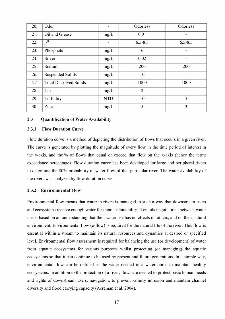
17
20. Odor - Odorless Odorless
21. Oil and Grease mg/L 0.01 -
22. pH - 6.5-8.5 6.5-8.5
23. Phosphate mg/L 6 -
24. Silver mg/L 0.02 -
25. Sodium mg/L 200 200
26. Suspended Solids mg/L 10 -
27 Total Dissolved Solids mg/L 1000 1000
28. Tin mg/L 2 -
29. Turbidity NTU 10 5
30. Zinc mg/L 5 3
2.3 Quantification of Water Availability
2.3.1 Flow Duration Curve
Flow duration curve is a method of depicting the distribution of flows that occurs in a given river.
The curve is generated by plotting the magnitude of every flow in the time period of interest in
the y-axis, and the % of flows that equal or exceed that flow on the x-axis (hence the term:
exceedance percentage). Flow duration curve has been developed for large and peripheral rivers
to determine the 80% probability of water flow of that particular river. The water availability of
the rivers was analyzed by flow duration curve.
2.3.2 Environmental Flow
Environmental flow means that water in rivers is managed in such a way that downstream users
and ecosystems receive enough water for their sustainability. It entails negotiations between water
users, based on an understanding that their water use has no effects on others, and on their natural
environment. Environmental flow (e-flow) is required for the natural life of the river. This flow is
essential within a stream to maintain its natural resources and dynamics at desired or specified
level. Environmental flow assessment is required for balancing the use (or development) of water
from aquatic ecosystems for various purposes whilst protecting (or managing) the aquatic
ecosystems so that it can continue to be used by present and future generations. In a simple way,
environmental flow can be defined as the water needed in a watercourse to maintain healthy
ecosystems. In addition to the protection of a river, flows are needed to protect basic human needs
and rights of downstream users, navigation, to prevent salinity intrusion and maintain channel
diversity and flood carrying capacity (Acreman et al. 2004).
Page 41
18
Environmental flow concept is at the core of all water management strategies for the river system
in Bangladesh. Because, investigation on e-flow requirements for rivers of Bangladesh is essential
in view of diminished flows and creation of dry beds in many rivers in lean seasons. The
environment itself is increasingly being considered as legitimate water user in many countries. As
a consequence the water requirement of the environment needs to be estimated. The amount of
water that has been allocated to the environment is a decision made by society, and is to some
extent arbitrary. Therefore, it has become essential to assess the e-flow for the sustainability of the
peripheral rivers and major rivers to use a source of supply for Dhaka city. There are numerous
methods available for the assessment of e-flows. The e-flow assessments (EFAs) are used as a
method for estimating the quantity of water required. The e-flow requirement for a river is the
minimum flow required to enhance or maintain aquatic and riparian life. More than 200
approaches have been used for determining e-flows in many different countries around the world.
The most commonly used method is the Tennant method or Montana Method ( Brij Gopal,2010).
This method is currently still the second-most widely used e-flow method in the world (Reiser et
al. 1989). It specifically links average annual flow to different categories of environmental habitat
condition. The Tennant method is based on discharge statistics and historical flows. The 10%
flow requirement for a watercourse is expressed as a percentage of the mean annual naturalized
flow at a specified site.
2.3.3 Use of Mathematical Model (HEC-RAS)
The mathematical model (HEC-RAS) developed by the Hydrologic Engineering Center (HEC) of
the US Army, is a modeling platform for simulating steady and unsteady flow conditions,
sediment transport (including mobile bed) processes and water temperature analysis. The HEC-
RAS system is comprised of a graphical user interface (GUI), separate hydraulic analysis
components, data storage and management capabilities, as well as graphics and reporting
facilities. The basic computational procedure of HEC-RAS for steady flow is based on the
solution of the one-dimensional energy equation. Energy losses are evaluated by friction and
contraction/expansion. The momentum equation may be used in situations where the water
surface profile is rapidly varied. These situations include hydraulic jumps, hydraulics of bridges,
and evaluating profiles at river confluences. For unsteady flow, HEC-RAS solves the full,
dynamic, Saint-Venant equation using an implicit, finite difference method. HEC-RAS is
equipped to model a network of channels, a dendritic system or a single river reach. Certain
simplifications must be made in order to model some complex flow situations using the HEC-
RAS one-dimensional approach (HEC-RAS, 2010). It is capable of modeling subcritical,
supercritical, and mixed flow regime flow along with the effects of bridges, culverts, weirs, and
Page 42
19
structures. Currently, the steady and unsteady flow hydraulic analysis components of HEC-RAS
are fully applied in practice. HEC-RAS model is therefore used to examine the scenario for the
determination of water availability in this study.
2.4 Review of Water Supply Assessment in Various Countries Lung W. S. (1986) developed a water assessment model for the upper James River to quantify
effect on growth of phytoplankton by phosphorus and other factors and to determine the impact of
point source phosphorus load reduction on biomass level. Variables considered in his model are
CBOD, DO, organic nitrogen, ammonia nitrogen, nitrite/nitrate nitrogen, algae and phosphorus.
Both BOD/DO kinetics and phytoplankton/nutrient dynamics are included in the model.
Calibration and verification reveal the few decisions. Light limitation causes unfavorable
conditions for algal growth which result in significant decline of phytoplankton biomass. DO
profile shows moderate depression below Richmond which is associated with BOD load from
point source and increase in algal photosynthesis. The lower level of orthophosphate in the James
River Estuary is about 0.01 mg/L of P, which is much higher than the limiting value of algal
growth. Phosphorus is not the key factor which limits phytoplankton growth in the river.
Turbidity, light, mean depth and all other factors govern in limiting phytoplankton growth in
James River Estuary.
Model projection indicated that reduction of phosphorus load from municipal waste water
treatment plant to levels that limit phytoplankton growth would facilitate the control of
phytoplankton biomass to reasonable and manageable levels. Modeling the phytoplankton
kinetics in relation to other system variables such as DO, CBOD, N, P, as well as light extinction
coefficient in the present study is expected to be performed in a similar approach adopted in this
paper. In addition, policy as well as waste management issues in the current study may be
addressed in a fashion similar to that adopted by Lung W.S. (1986).
Badruzzaman, A. B. M. and Lung W. S. (1991) developed a 3-D multilayered time variable
model to assess the temporal and spatial distribution of dissolved and particulate Cu (II) in water
and sediment layer. The author mentioned that a significant amount of pollutant have been
introduced into New York Bight for past 30 years. These are originated from transact zone which
includes New York metropolitan area, Northern New Jersey and Hadson river drainage basins
which causes accumulation of Cu(II) in water and sediment layer. Their model incorporates the
physical process of advection-dispersion and settling, chemical processes of sorption,
Page 43
20
precipitation, speciation and bio-uptake. The model developed in their study includes two sub
models one deals with transport fate and the other addresses metal chemistry.
In the model the water column is considered to be divided into 02 layers to represent seasonal
stratification in which less dense water from Hadson-Raritan estuary flows outward through the
upper layer and dense Bight water flows through the lower layer. The advective-dispersive
transport of Cu (II) is handled by the WASP and a kinetic submodel is structured to handle the
kinetic transformation processes such as adsorption, bio-uptake, bio-turbulation and sediment
burial. From the schematic representation of the processes involved in Cu(II) distribution, there
were the few conclusions. The aerobic sediment layer is considered to have diffusive exchange of
dissolved Cu (II) with both overlying water column and the underlying anaerobic sediment layer.
The particulate exchange in the water column is a function of advection and dispersive transport
and loss due to settling. The top sediment layer is assumed to have no accumulation or loss of
particulate. The bottom layer of sediment is assumed to receive the settling solid particulate from
water column and suffer due to particulate leaving the layer through sedimentation. The model
developed was run with different sets of data and they were well reflected by the model which
shows the following results. A seasonal rise and fall of metal concentration occur in the water
column. Initially more accumulation of Cu (II) in the sediment layer, but after some time, bio-
turbulation mixing causes more polluted particles to be brought into the top sediment layer from
the bottom layer and dissolved Cu (II) in the same layer increased because of Metal diffusion.
Sensitivity of their model is also tested by varying different key parameters such as settling
velocity, loading and vertical diffusion coefficient. Decreased concentration of particulate Cu (II)
in the water column and increased concentration of particulate Cu (II) in the sediment layer
occurs because of doubling the settling velocity. Increased concentration of both dissolved and
particulate Cu (II) in the water column and no change in the sediment layer occurs because of
doubling the load. The reason behind this is that the water column reaches equilibrium much
faster than sediment layer.
When vertical diffusion decreased to 1/10th of its initial value between the surface and bottom
layer, the dissolved Cu(II) diffused into the bottom water layer and remain entrapped there
increasing concentration. The study also shows that chemical speciation of Cu (II) is depended on
its concentration in water and sediments and at low concentration, only one species dominates. At
higher concentration, chemical reactions produce species reducing the dominance of one species.
Page 44
21
Bongartz et al. (2007) dealt with water characterization (assessment) and load-reduction impacts
evaluation (modeling) of stream water quality data in the Saale River basin, Germany. For a
period of 6 years the data which was sampled by government environmental agencies was
investigated to assess indicators and sources of pollution. The investigation has shown that some
selected water quality parameters can be used as catchment specific indicators for different kinds
of pollution and differentiate between human made and natural sources. Thus, management
measures which are required by the European Water Framework Directive (WFD) can be applied
according to the specifics of the various sub-catchments with pollution hotspots. The assessment
of sources of pollution via a modeling (using WASP5) exercise of the routing of different
pollutants was made in the lower part of the basin. The modeling was done to evaluate not only
the sources of the pollution but also the distribution and the accumulation within the stream
network. The method used to analysis the load-reduction impacts in this paper may be adopted to
conduct similar analysis in the current study. Liao and Xu (2008) hydrodynamic and water quality models of Suzhou Creek were developed.
Based on models, the impacts of the upstream input and local pollution loads were analyzed. The
water quality of Suzhou Creek was predicted based on the assumption that the upstream quality
was improved by one class and the tributary quality met Class V of the National Surface Water
Quality Standards. The relative ratios of tributaries meeting Class V to upstream improvement for
the water quality improvement of Suzhou Creek were also computed. From the above analysis,
the authors drew the few conclusions. The change of the water quality of upstream input impacts
more on the upstream segments of Suzhou Creek than the downstream segments. Among all
monitoring parameters, DO is most sensitive to this change. On average, the local pollution loads
impact the water quality of Suzhou Creek slightly more than the upstream input.
2.4.1 Water Demand Management in Srilanka
Srilankan water management strategies are recommended by several studies as follows:
a. Per capita consumption to be reduced from 145 lpcd to 120 or 100 lpcd by tariff itself.
b. Rainwater harvesting for urban users.
c. Promotion of alternative water uses- recycling of wastewater from industrial sector and
use of separate system for gardening etc.
d. Creation of awareness among users
e. Public Participation
Page 45
22
2.4.2 Water Supply Management in India
Water scarcity is a prime issue in Dwarka municipality in India. Dwarka district is in the Gujarat
state in north-western India. Dwarka is getting around 25% of their demand from the Delhi
Development Authority (DDA). So there is huge demand supply gap. In order to cope with
inadequacy of service utility, several strategies have emerged at the individual and community
level. Some of these strategies are discussed are follows:
a. The authority offered linear solution, withdrawing increasing volume of water and
discharging waste at ever increased levels. It caused escalating stress on receiving
environment. This approach is towards increasing the quantity of supply.
b. To make water management sustainable urban water management must integrate a larger
proportion of solutions like raising awareness to reduce consumption, law enforcement
and controls, reuse and recycling of storm-and wastewater, and climate change adaptation.
c. Raising awareness on water risks, efficient water used through the stakeholders’
involvement in water management. Identification of key actors and their role in water
management must be investigated for sustainable water management.
d. The development control, policies, laws enforcement situation must be investigated. The
estimated breakup of the per capita water demand clearly shows that 40% of the domestic
demands in Delhi need not to be potable water and recycled greywater can be used which
can be applicable for Dwarka also. The Central Groundwater Authority made it mandatory
for buildings (for plot area 100 m2 or more) in Delhi to make provision for rainwater
harvesting. The byelaw is applicable for Dwarka also; however the implementation of the
same is not being monitored by the government concerned agencies and its technological
appropriateness and maintenance is doubtful.
e. The Delhi Government has modified the building byelaws (GOI notification 28 July 2001)
to promote reuse of wastewater in buildings where daily wastewater generation is 10,000
litres or more. DDA initiated use of dual water supply systems in Dwarka in 2002-03 to
promote the reuse of rainwater and recycled wastewater.
f. The Master Plan for Delhi 2021 has also emphasized the recycling of treated wastewater
through dual supply systems, however, these concepts have not been implemented in
Dwarka until today. Government agencies also have not taken any action to implement the
act because they are not clearly aware of the technicalities for the system. The area has
been notified which means no groundwater extraction is permitted unless approved by the
Central Water Government Authority. However, it is a known fact that there is rampant
illegal boring in the area.
Page 46
23
g. The National Water Mission has given emphasis on the water use efficiency, exploring the
option to augment water supply in critical area, this mission strategies also include studies
on the management of surface water sources, management and regulation of ground water
sources, upgrading storage structures for fresh water and drainage systems for wastewater,
conservation of wasteland and development of desalination technologies. The National
Mission on Strategic Knowledge for Climate Change tends to identify the challenges of
and the response to climate change through research and technology development.
Applicability of these missions’ strategies for Dwarka is necessary for sustainable water
management.
2.4.3 Water Management in Nepal
This large scale wastage of the surface water flow is true in Nepal because out of 225 billion
cubic meter of annual surface flow, only 2% is utilized in the country and the rest drain down to
Indian plain passes through the large Gangetic plains of India and enters Bangladesh before it
finds drain down to the Bay of Bengal and join the sea. On the other hand, acute water shortage is
being felt in several part of the country. It is therefore imperative to develop additional storage in
the country to reduce this wastage to as low as possible. Nepal consists of about 80% of
the mountainous area, the rest being plains and lowland. It consists of the three roughly parallel
strips namely the northern region of the high mountains, central region and the southern region of
Terai. Nepal is under the general influence of the sub- continental climatic pattern. It has two
distinct seasons. Different water resources available in Nepal are summarized below:
a. Depending on the sources of the discharge, the rivers of Nepal are of three grades. The
first grade rivers are the Karnali, Narayani and the SaptaKoshi along with their tributaries,
having their sources in the snow and glaciers in the Himalayan Region. There are about
6000 rivers in Nepal. 1000 of which are more than 11 kms long and about 100 of them are
longer than 160 kms. The total length of all streams and rivulets exceeds 45,000 km.
b. Although ground water resources are still under investigation in Nepal, so far the most
prospective sites of the ground water resources lying mostly in the Terai and in some
mountainous valleys as well. Static water tables of the aquifers lie normally between 3 to 10 m
from the ground surface in the eastern and Central Terai with yield between 100-300 cu m/hr.
c. There are innumerable lakes and ponds, covering about 2% of the total runoff. Most of the
oxbow lakes are found in Terai. There are several hot springs known as " Tatapani" and
similarly hot suppurated water exists about 1 km south of kowaris check post in Sunkoshi
valley. In Janakpur also there are three hot springs containing sodium, potassium,
Page 47
24
sulphate, carbonate and chlorine ions. Water is mainly used in Nepal for the agricultural
domestic, industrial and the commercial purposes. About 80% of the people in Nepal are
engaged in Agriculture. Due to the shortage of water problem, in drinking water, for
domestic use, for the irrigation, fisheries hydro power, industrial work, infrastructure
development and ultimately affected the human existence. The activities like discharging
domestic sewage & sludge, industrial effluents, agricultural chemicals and the solid
wastes, encroaching riverbank for illegal settings, pig farming, vehicle repair and
slaughter of animals, all these contribute to the pollution of water resources and poor
water quality. To utilize the natural resources for the maximum benefit of the human being
it is essential that proper managing of the natural resources should be made.
d. One way to manage water resources is to increase the supply in a particular area by
building dams & reservoirs, bringing in surface water to form another area or tapping
ground water. Another approach is to improve the efficiency of the water use. Solutions
adapted by Nepal to restore the available water resources and managing water can be
discussed in following points:
e. Huge dams and reservoirs have benefits & drawback, water from rain & melting snow can be
captured and stand in large reservoirs created by damming streams. This water can then be
released to produce hydro-electric power at the dam site, to irrigate land and to provide water
carried to towns and to provide water carried to towns and the cities by the aqueducts.
Reservoirs are also can be used for the recreation activities such as swimming, fishing, boating.
f. Groundwater should be tapped for the solving water problems. Ways to slow groundwater
depletion include controlling population growth, not planting water- thirsty crops in dry
areas, developing crops strains that require less water & wasting less irrigation water.
2.4.4 Surface Water Management Plan (SWMP) in London
London has a SWMP with the purpose of sustainable surface water management decisions that
are evidence based and risk based, whilst taking climate change into account, and are inclusive of
stakeholder views and preferences. The framework for undertaking a SWMP study is illustrated
through a wheel diagram, identifying the four principal phases: Preparation; Risk Assessment;
Options; and Implementation and Review. The first three phases involve undertaking the SWMP
study, whilst the fourth phase involves producing and implementing the action plan, based on the
evidence gained from the SWMP study. It was based on a widely adopted generic approach to
evidence and risk based decision making (Arthington et al. 1998). The phases are summarized as
follows:
Page 48
25
a. The first phase of a SWMP study focuses on preparing and scoping the requirements of
the study. Initially, partners and stakeholders should identify the need to undertake a
SWMP study. The aims and objectives of the study should be established, and in parallel
the partnership will also decide how they will engage with stakeholders throughout the
SWMP study. An assessment should subsequently be undertaken to identify the
availability of information. Based on the defined objectives, current knowledge of surface
water flooding, and the availability of information, partners should agree the level of
assessment at which the SWMP study should start.
b. The outputs from the preparation phase will identify which level of risk assessment will
form the first stage of the SWMP study. The first stage is likely to be the strategic
assessment where little is known about the local flood risks. The strategic assessment
focuses on identifying areas more vulnerable to surface water flooding for further study.
The intermediate assessment, where required, will identify flood hotspots in the chosen
study area, and identify quick win mitigation measures, and scope out any requirements
for a detailed assessment. A detailed assessment of surface water flood risk may be
required to enhance the understanding of the probability and consequences of surface
water flooding and to test potential mitigation measures in high risk locations. Guidance is
provided on undertaking modelling to support a detailed assessment of surface water flood
risk and mitigation measures. The outputs from the strategic, intermediate and/or detailed
assessment should be mapped and communicated to all stakeholders including spatial
planners, local resilience forums, and the public.
c. In this phase a range of options is identified, through stakeholder engagement, which
seeks to alleviate the risk from surface water flooding in the study area. The options
identified should go through a short-listing process to eliminate those that are unfeasible.
The remaining options should be developed and tested using a consideration of their
relative effectiveness, benefits and costs. The purpose of this assessment is to identify the
most appropriate mitigation measures which can be agreed and taken forward to the
implementation phase.
d. Phase 4 is about preparing an implementation strategy (i.e. an action plan), delivering the
agreed actions and monitoring implementation of these actions. The first step is to develop
a coordinated delivery programme. Once the options have been implemented they should
be monitored to assess the outcomes and benefits, and the SWMP should be periodically
reviewed and updated, where required. In Figure 2.1 shows the diagram connecting the
coherence in plans and policy.
Page 49
26
Figure 2.1: Diagram showing the coherence in plans and policy (Arthington et al. 1998)
2.4.5 Surface Water Management Plan in New York, USA
The Bureau of Water Resource Management works to protect, manage, and conserve New York
State's groundwater and surface water supply sources, develop management strategies to enhance
and protect these waters, and protect both the groundwater and surface water quality in the New
York City Watershed and other major watersheds (Deniz et al. 2004).
a. The Bureau's work includes programs for public water supply permitting, which
includes analysis and approval of aquifer (pump) tests and reservoir capacity; drought
management; Great Lakes water withdrawal registration; statewide water withdrawal
reporting; groundwater; interstate water supply partnerships; reservoir releases; water
conservation; and water well drillers registration. The Bureau provides geotechnical
assistance to local, state, federal, and industrial/commercial entities, and has partnered
with the U.S. Geological Survey (USGS) for over 25 years to conduct a cooperative
statewide aquifer mapping program.
b. The Bureau also manages DEC's water quality and watershed protection programs for
the New York City water supply system, including Federal Safe Drinking Water Act
grants, compliance for SPDES permits within the watershed, and technical assistance
and training for wastewater treatment facility operators within the watershed.
c. The Bureau works with stakeholders and partners to improve water quality, provides
funding for Water Quality Improvement Projects, and conducts outreach and
communication activities. The Bureau's responsibilities also include developing and
managing a geographic information system (GIS) that provides information and data
Page 50
27
about New York State's waters.
d. Bureau Sections includes four sections as:
Water Quantity Management Section
New York City Watershed Section
Watersheds Program Coordinator
Non-Point Source Section
2.5 Water Supply Scenario in Different Cities
Water supply circumstances are diverse for various cities and countries. Different cities possesses
different scenario regarding water supply. The scenario reveals an impression that average
number of person per connection is more in Dhaka than other cities as shown in Figure 2.2 as
well as Table 2.2.
Figure 2.2: Water supply scenario in different cities
Table 2.2: Water supply scenario in different cities
City
Average number of persons per connection
Percentage with 24-hour Supply
Per capita consumption (lcd)
Dhaka 30 0 117
Kathmandu 10.5 0 69
Manila 9 97 127
Ho Chi Minh 8.75 75 168
Jakarta 7.5 90 76
Phnom Penh 7 100 104
Colombo 6 60 119
Vientiane 6 50 112
Delhi 5 1 109
Karachi 5 0 198
0
50
100
150
200
250
Wat
er C
onsu
mpt
ion(
lcd)
Average number of persons per connectionPercentage with 24-hour supplyPer capita consumption (lcd)
Page 51
28
2.6 System Loss in Different Cities System loss is a serious issue in water supply sector. It may not be stopped but it can be
minimized. System loss is also prevailing in other countries. However for the Dhaka city the
system loss is quite similar to the other neighboring countries (Lung, 1986). Necessary steps must
be taken to reduce the system loss to make it more rational. As for examples, system loss in
percentage in some cities of neighbouring countries is shown in Figure 2.3.
Figure 2.3: System loss in cities of neighboring countries
2.7 Review of Studies on Surface Water Quality of rivers around Dhaka City
Many works have been conducted on the surface water sources of rivers around Dhaka city.
Reviews of some of the recent studies on surface water sources from Padma, Meghna and
peripheral rivers around Dhaka city works have been performed. Haque A (2014) in his article
reported that water management in Dhaka city has become a megacity with a population of nearly
15 million, which is increasing at an annual rate of over 5%. Industrial, domestic and commercial
wastes are polluting surface water, and groundwater in certain areas of the city also shows signs
of both organic and inorganic contamination. Laws to prevent environmental pollution are rarely
enforced. Overall service delivery considered to be poor due to an inadequate tariff structure, high
non-revenue water, lack of authority and commitment, inadequate management capacity, lack of
sector coordination, inadequate investment, absence of effective decentralization etc. He also
focused that the situation could be improved by higher investment, effective private sector
participation, improved billing and revenue collection, structural reforms, establishing a
regulatory body and finally converting DWASA into a truly service oriented commercial
organization. The performance of DWASA needs to be improved to meet the millennium
development goals. He also mentioned that millennium goals can be achieved by reducing the
population without access to water supply and sanitation services by 50% by the year 2025.
0%
5%
10%
15%
20%
25%
30%
Syst
em lo
ss in
% Systems loss
Page 52
29
Karim et al. (2000) carried out field monitoring and laboratory measurement of water availability
and quality of the lower reach of the peripheral rivers for the month of January to April. He
applied 1-D WASP (Water Quality Analysis Simulation Program) by the USEPA with the
collected data to quantify the state of pollution and the assimilative capacity of the river for dry
weather condition. It was reported that the DO condition of the river water remains above the
critical level of 4.0 mg/L, supporting the survival of aquatic life including fish. He found that the
river had significant assimilative capacity and can assimilate the waste load from future new
industrial establishment without violating the DO standard under prevailing flow condition.
However, some water quality parameters like total nitrogen and suspended solids would remain
very high and cause a potential threat to the aquatic life. He stressed that necessary management,
control of projected waste loadings and ensuring current river flow must be formulated to support
balance aquatic life and increased river assimilative capacity. His study revealed that
phytoplankton growth in the river is highly suppressed due to the lower level of light penetration
caused by high turbidity in the water column.
For the feasibility study of Saidabad Water Treatment Plant, IWM (2004) analyzed the water
quality data of Sitalakhya and the Balu river. Water samples were collected from 4 locations
along the Sitalakhya river from Ghorasal to the Sarulia intake point during high tide to obtain an
idea about the distance to which the polluted water from the Balu-Sitalakhya confluence travels
upstream during high tide. The water samples test results showed high contents of ammonia upto
around 3 km from the confluence. Based on available data they found that the Balu river with
very low DO and high coliform values, especially during the dry season, appears to be more
polluted than the stretch of the Sitalakhya river. The main concern for the Saidabad water
treatment plant during the dry season is the high concentration of ammonia and algae in the intake
water. To find out an alternative location, they also analyzed Majhina about 1 km south of
Rupganj ferry-ghat for projected BOD loadings. BOD loadings were estimated for the years 2000,
2005, 2010, 2015, 2020 and 2025. Model results showed that DO level increases from the Sarulia
intake towards upstream direction. DO level at Sarulia intake point goes down to 1.0 mg/L for
2002 loading and it further goes down and reaches to 0.67 mg/L for 2025 loading conditions. The
DO level near village Atabo (1 km u/s of Rupganj Hospital) remains always above 4.0 mg/L for
all loading conditions. DO level at proposed intake location goes down to nearly 3.0 mg/L for
2025 loading condition. They concluded that there was no significant deterioration in DO level
from the Majina location which was more preferable than Atabo.
Page 53
30
Ahmed, T. (2005) investigated the effects of thermal discharges in the Sitalakhya River from the
existing and proposed thermal power plants in the Siddirganj area. The CORMIX model was used
for prediction of thermal plume for discharges of Siddirganj and Globeleq power plant under
different tidal conditions of the river during the critical dry period of the river. Water quality
simulation results of some parameters such as BOD, DO, ammonia, nitrate, phosphate was carried
out for existing conditions of the river. Sensitivity analysis was performed to assess the impact of
excess temperature caused by the thermal effluents from the power plants. The results of the
analysis showed a small decrease in BOD and ammonia, a small increase in nitrate and a
significant decrease in DO (about 0.5 mg/L) due to excess temperature.
Majumder, T. K. (2005) overviewed contamination scenario of the peripheral river system around
the Dhaka city including historical trend of the pollution. It was observed that required DO for
sustaining aquatic lives (4 mg/L) prevails only in the Dhaleswari River and in a very short
downstream reach of the Sitalakhya River throughout the year. The rest of the river reaches
maintain lower DO level, usually less than 1 mg/L, in the dry period. Ammonia level in different
reaches of the river system is well above the permitted value in the USEPA guideline to avoid
toxic effect on fishes. Concentrations of Nitrate, Phosphate, Zinc, Chromium, Lead and Mercury
in the river system are well below the allowable limits specified in different Environmental
Quality Standards (EQS).
The study findings highlights that it is essential to make provisions for improving water quality in
the peripheral rivers to sustain the city water supply system, the ecosystem in the rivers and,
above all, the overall environment of the capital city. Further detail study carried out by IWM
(2006) to assess the water of the major rivers with special reference to the intake point of
Saidabad water treatment plant. Following results have been found from the analysis:
a. Water quality at the intake point at Sarulia is highly polluted. The DO level in present
condition (0.6 mg/L) was far below the critical DO level (4 mg/L) and it continued to
decrease with increasing waste load in future. The water quality of Sitalakhya river in the
upstream of Sarulia was much better and at 7.5 km upstream it was very close to the
critical DO value.
b. The Norai khal, which falls into the Balu river at 5.5 km upstream of the Balu-Sitalakhya
confluence, is chiefly responsible for deteriorating the water quality of Balu river. Norai
khal effluents also affect the water quality at Sarulia as Sarulia is only 400 m downstream
of the Balu-Sitalakhya confluence.
Page 54
31
c. In addition to Norai khal, DND khal, Majheepara khal, Tanbazar khal, Killarpul khal,
Kalibazar khal and B.K. Road khal from Narayanganj area are identified as the major
pollutant sources affecting the water quality at Sarulia.
d. On the basis of their analysis, finally they recommended that of the state of water quality
major sources should be treated before their disposal to rivers.
Department of Environment (DOE, 2016) assesses the surface water and ground water resource
throughout the country almost every year. The main objective of the campaign was to investigate
the existing condition of the water bodies in Dhaka city. Water quality of peripheral rivers of
Dhaka was measured at different sampling stations in the year 2010. The sampling stations of
DOE are located at different locations of peripheral rivers. The main objective was to create a
database of water quality of peripheral rivers around Dhaka city. Following Table 2.3 shows the
state of water demand against the population and the amount of deficit occurs in percentage
(DWASA, 2014). It represents that the deficit gradually increases with the increase of population
and demand.
Table 2.3: Population, water supply and demand for various years
Year Population (millions)
Water Demand (MLD)
Water Supply (MLD)
Deficit (%)
1963 0.85 150 130 13
1970 1.46 260 180 30
1980 3.03 550 300 45
1990 5.56 1000 510 49
1996 7.55 1300 810 38
1997 8.00 1350 870 36
1998 8.50 1400 930 34
1999 9.00 1440 1070 26
2000 9.50 1550 1130 25
2001 10.00 1600 1220 24
2002 10.50 1680 1300 23
2003 11.00 1760 1400 20
2010 12.27 2485 1500 40
2020 18.04 3680 1500 59
Page 55
32
2.8 Review of Previous Studies on Groundwater Quality
As stated earlier 78% of Dhaka city water supply is dependent on ground water sources.
However, ground water sources are at the verge of contamination as reported by many reseschers.
The outcomes of the works are summarized as follows:
There are around 702 DTWs in the upper and lower aquifer of Dhaka city. Every year the
groundwater level is depleting at a rate of 2‐3min the upper dupitila aquifer. A study by IWM that
the rate of mining of the upper dupitila aquifer is around 14‐15% and the potential of exploitation
of the lower dupitila aquifer is limited. Therefore, the groundwater aquifers are no longer
sustainable in the long‐term identification and utilization of alternative sources to groundwater is
very important to meet the water demand of Dhaka City (IWM, 2014). A project is being carried
out by DWASA which will bring 300 MLD of groundwater in two phases from a well field in
Savar and Singair Upazilla. The most critical period of the year is March in terms of water
availability and water quality for the surface water sources. Therefore assessment of water
availability was made based on historical simulated data from March. It was found that
withdrawal for water supply from the peripheral Rivers would not result in any major change in
water depth. But the water quality is progressively declining due to increase in pollution load
from various domestic and industrial sources. The situation would further deteriorate if no
pollution control measures are implemented. Therefore, the peripheral rivers as water supply
sources for Dhaka city are considered vulnerable. Water availability analysis in the major rivers is
show that they have significant flow available. The water quality of these rivers is also acceptable.
The feasibility studies of the Gandharbapur SWTP and Saidabad Phase‐III found abstraction of
2525 MLD water is viable from Meghna River. The feasibility studies of Jashaldia SWTP found
abstraction of 900 MLD is viable from Padma River. These sources have been found to be
technically and economically feasible in the long‐term for Dhaka City. Additional analysis has
been done for resource assessment periods 2035 to 2060. The availability of suitable water from
the Meghna River for additional use has some uncertainties. However, the Padma River should be
a reliable source. Protection from pollution is required if peripheral rivers are to be considered for
future supply.
Based on the monitoring and chemical analysis of samples from groundwater wells (both HTW
and DTW) all over the Dhaka city a general trend of increasing groundwater pollution has been
identified from north to south of the city. The wells near the Buriganga River has been found to
have very high concentration of Cl-, SO4-2 and NO3
- while these are present in very small quantity
in the wells in the northern part of the city. Presence of considerably high quantity of these three
Page 56
33
ions in the wells near Buriganga suggests infiltrating surface water may contaminate the
groundwater. A zone of relatively elevated groundwater Electrical Conductivity (EC) is apparent
in the southern part of the city and this has migrated progressively towards north from 2012 to
2014 (Hasan et al. 2014).
Ahmed et el. (2012) conducted a study for the assessment of ground water quality on the Jatrabari
area, waste dumping site. He showed that a significant depth variation in groundwater EC. The
HTW water is characterized by high concentration of dissolved ions including Cl- than the DTW
water. Industrial effluent dumping sites; the Begun Bari khal at Tejgaon, Dholaikhal at
Dholaikhal engineering workshop area, Hazaribaghkhal and Buriganga at Hazaribagh tannery are
causing groundwater pollution. The impact of effluent and polluted river water is more
pronounced in shallow groundwater (<100m) as compared to deep groundwater. EC of shallow
groundwater well at Hazaribagh was 1000 S/cm whereas the EC of DWASA production well
was 650 S/cm.
An assessment of groundwater contamination by (Karim et al. 2000) revealed that higher
concentration of chromium had been detected in the samples from Zone 2 compared to other
DWASA zones where tannery was located. It is also reported that the average chromium
concentration of the 14 water samples from Zone 2 is 0.036 mg/l and the concentration varies
significantly with time. As no natural source of chromium is present, chromium rich tannery
wastewater appear to be the most likely source of chromium in groundwater. But the seasonal
variation of chromium is not clear. Apart from chromium, alarmingly high lead concentrations
were found in many DWASA groundwater samples of Zone 2. Most of the samples exceeded
WHO guideline value for drinking water (0.01 mg/l). This is a serious health concern and should
be addressed immediately. It also reveals that significant levels of Sulphide is also detected in
samples of Zone 2 but not detected in the samples from other zones except in few from Zone 4. It
also appears that the tannery wastes are responsible for high sulphide concentration. Literatures
reviewed on groundwater quality of Narayanganj area reveals the state of groundwater quality of
the Narayanganj area in the recent years and the possible causes of groundwater deterioration.
High groundwater EC values (1000 to 2900 S/cm) detected in the central and southern part of
the city, close to Sitalakhya River shows marked vertical variations in groundwater quality.
Shallow groundwater has higher dissolved solids, which demonstrates contamination in the upper
aquifer. Several heavy metals: As, Pb, Mn, Cd are found to occur above the Bangladesh and the
WHO drinking water standards in a number of samples tested. Highest concentration found was
0.075 mg/l at a HTW in Kadamrasul area of the town. The possible causes of groundwater quality
Page 57
34
deterioration for the Narayanganj area other than arsenic are Industrial contaminants, land filling
with municipal wastes, discharge and leakage from open drains and septic tanks.
2.9 Deep Tube Wells Operated by Private Agencies
At present around 1846 DTWs are operated by private agencies (DWASA, 2016). Commercial
and industrial sectors are the major stakeholders of this group. DWASA does not have any
statistics on the actual water extraction through these DTWs (Serajuddin, 2014). It is identified as
a grey area of the overall water supply system of the city. A lot of steps were taken to explore the
water consumption data of the garment industries alone. From BGMEA it was found that, at
present total 1600 garment factories are operational in the city. The average water consumption to
produce a finished 1 kilogram knitwear and woven product is around 115 liters and 130-140 liters
respectively. From Export Promotion Bureau it was found that, total 508.67 million pieces of
knitwear and 484.95 million pieces of woven products were exported during the year 2013-2014
(Bhuiyan, 2014). No data in terms of volume or weight of the total production is available with
any of the organizations. As a result, correlation between water consumption and total production
was not possible and no conclusive remark could be made on total water consumption. However,
it is perceived that, huge amount of groundwater is extracted by these types of users which need
to be identified and monitored for sustainable and efficient planning.
2.10 Relevant Studies of Dhaka Water and Sewage Authority (DWASA)
DWASA collected water sample from peripheral rivers and analyzed water quality parameters in
their laboratory. They observed that most of the water quality parameters are quite higher than
the guideline value. Thus the surface water quality was not found suitable for both domestic and
agricultural use with a very little exception like Dhaleswari and Shitalahkya river throughout the
year.
Institute of Water Modeling (DWASA, 2014) conducted feasibility study for the rehabilitation of
Buriganga-Turag-Shitalakhya river system and for the augmentation of dry season flow in the
Buriganga river. The study suggested that the project will take long time to implement and thus
not cost effective.
Rahman S (2005) made a study on water quality parameters of peripheral rivers of Dhaka city.
From the study, it was found that rivers were not suitable as a source of water supply for Dhaka
Page 58
35
city in the dry season. However, in wet season the water quality parameters were found
satisfactory.
BWDB reviewed surface water quality data of peripheral rivers of Dhaka with their 17 sampling
stations and their altogether 38 sampling stations of different organizations including DPHE, and
DWASA. They concluded that surface water quality in most part of Dhaka is not suitable for all
uses (BWDB, 2009). At that time they gave aesthetic issue of iron, chloride, TDS and hardness.
There review neither reported to show its suitability for domestic purpose.
Institute of Water Modeling (IWM, 2005) carried out an investigation on the water quality of
Shitalakhya river at the locations adjoining the Saidabad Surface Water Treatment Plant (SWTP)
in 2005. The report is focused on the water quality of Shitalakhya river close to the intake point of
Saidabad Surface Water Treatment Plant (SWTP) to justify whether the intake point is in suitable
location for water supply or not. The report found out that the intake point is in the suitable
location.
Considering the existing groundwater situation, DWASA is making a strategic effort to build
more surface water treatment plants (SWTPs). Currently, there are 4 SWTPs in operation.
Sonakanda SWTP is currently being rehabilitated and the new plant will have 12 MLD capacity.
Godnail SWTP is currently production 18MLD but after renovation works it will have 45 MLD
treatment capacity. Chandnighat SWTP has a capacity of 39 MLD after renovation work but
produces 1 MLD on an average during dry seasons due to low water levels in Buriganga River.
Even the treated water at the plant cannot meet the WHO and Bangladesh standard due to poor
intake water quality. In fact, all four SWTPs suffer this problem. Of the existing 4 plants,
Saidabad SWTP Phase-I plant is the largest and it has been operating since early 1990s, while
Phase-II plant became operational in December 2012. The objective of 1 bar pressure at the
farthest point of the main is yet to be realized. Godnail and Sonakanda SWTP Transmission Main
is currently undergoing rehabilitation (35km) and 60 km new mains of diameter 150 mm to 800
mm are being constructed. New primary and secondary distribution mains for the proposed
SWTPs will also be required.
The network suffers from lack of proper planning, ageing fixtures, poor material and poor
workmanship. The system also suffers from illegal connection and pilferage. The District Metered
Area (DMA) program plans to rehabilitate and replace the existing distribution network. DMA is
designed to be a 24 hr pressurized system that will source water from local DTWs and SWTPs i.e.
conjunctive usage. However, given the uncertainty associated with DTW supply due to
Page 59
36
mechanical and electrical failure of DTWs; the 24hr continuous pressure condition in the network
will be a challenging proposition to realize in a different situation (IWM, 2014).
DWASA prepared water supply master plan (2014), a set of guiding principles were discussed
regarding water quality and availability. It was proposed to build the capacity of the organization
should be enhanced for future requirements. Master plan also focused on improving coordination
between stakeholders, efficient management of assets and human resources. Reduction of ground
water use, protection of water supply sources to ensure pressurized water supply distribution and
identification of future urban expansion areas is also suggested in Master plan. In addition to
improving overall efficiency of operation and maintenance (O&M), the master plan suggested to
reduce non-revenue water and power consumption. Emphasis is also given to develop strategic
plan for efficient water utilization and promotion of water use conservation for demand
management. Master plan also focused on collection of revenue opportunities and collection
efforts need to be improved. For implementation of the master plan, capital expenditures
(CAPEX) needs to be clearly identified and potential funding sources have to be indicated. The
annual budget and O&M plan needs to evaluated and tariff needs to be set for DWASA
accordingly. It may be necessary to establish interim objectives that ensure a gradual progression
to full cost recovery over the years. The overall environmental condition of Dhaka is increasingly
reaching a critical situation which is mainly due to a very dense population with high growth
rates, and limited water distribution coverage for the city. On the other hand, Bangladesh is
already committed to improving the water and sanitation scenario of its urban settlements. MDG
was targeted by 2015. This commitment is further reinforced due to its policy of achieving
Sustainable Development Goals. The SDG (https://unstats.un.org/sdgs/files/metadata-
compilation/Metadata-Goal-6)has the following water related goal specified:
a. By 2030, improve water quality by reducing pollution, eliminating dumping and
minimizing release of hazardous chemicals and materials, halving the proportion of
untreated wastewater and substantially increasing recycling and safe reuse globally
b. By 2030, achieve access to adequate and equitable sanitation and hygiene for all and end
open defecation, paying special attention to the needs of women and girls and those in
vulnerable situations.
c. By 2030, achieve universal and equitable access to safe and affordable drinking water for
all.
d. By 2030, substantially increase water-use efficiency across all sectors and ensure
sustainable withdrawals and supply of freshwater to address water scarcity and
substantially reduce the number of people suffering from water scarcity.
Page 60
37
e. By 2030, expand international cooperation and capacity-building support to developing
countries in water- and sanitation-related activities and programmes, including water
harvesting, desalination, water efficiency, wastewater treatment, recycling and reuse
technologies.
f. By 2030, implement integrated water resources management at all levels, including
through transboundary cooperation as appropriate.
The Master Plan aims to achieve these goals in the context of water supply in Dhaka city.
Moreover, more reliance is given on large rivers than the peripheral rivers. The emphasis was
given for collection of surface water from large rivers specially from Padma and Meghna.
However, detail study was not conducted on peripheral rivers for the assessment of potential
sources of surface water for Dhaka city (IWM, 2014).
2.11 Management Plan for Water Supply Project
2.11.1 Demand and Supply Side Management
The Dhaka water supply authority is considering exorbitantly expensive option of bringing raw
water from distant rivers like the Meghna or the Padma, which is unlikely to be a sustainable
option. Strategically therefore, abating pollution of the Balu-Sitalakhya river system including the
internal conveyance canals through a combination of pollution prevention and control measures at
different sources would be much more cost effective and sustainable solution. Similar approach is
also to be considered for the Turag-Buriganga-Dhalswari river system (DWASA, 2014).
2.11.2 Water Reuse
The general principles and technological developments of water reuse and renovation can be
discussed as follows:
a. With the technological advancement and public acceptance, greywater seems to be a
potential source of water saving. Traditionally, greywater is defined as non-industrial
wastewater generated from domestic processes such as dish washing, laundry and bathing.
Essentially, any water, other than toilet wastes, draining from a household is greywater.
b. Greywater is a major fraction of domestic wastewater which is generally less polluted than
other types of wastewater. Burnat et al. (2007) reported that the amount of greywater
produced in household is 55% - 65% of the total amount of wastewater. This water
generated from sinks, baths, showers, or washing machines. This water can be treated
onsite or offsite for non-potable use purposes such as irrigation, toilet flushing, car
washing, dust control, soil compaction, in construction works and in industrial processes
Page 61
38
like cooling boilers and other appliances (Almeida et al. 1999). Reuse of greywater in
toilet flushing and gardening can save 31-54% of potable water in households. Water
reuse in long term will reduce the water demand and finally meet the requirement of water
in 2035.
2.11.3 Pollution control
The tanneries are responsible for causing pollution in the Buriganga River by the contribution of
toxic and persistent pollutants. Every kind of pollution making industry including tannery should
be uprooted from both sides of the Buriganga River. Proper treatment plant of sewage needed
before sewage disposal in the Buriganga, Shitalakhya, Turag, Balu River and Tongi Khal for that
pollution making industry should have effluent treatment plant (ETP).Dissolved oxygen (DO)
data measured is available only for 8 hours or less in a day which is insufficient to understand the
complete diurnal variation. Continuous measurement of DO throughout the whole day or at least
12 hours will help to understand the complete diurnal variation. Proper laws should be enforced
from the Department of Environment to reduce the pollution of the river water from adjacent
pollution. New and old industries must be regulated under pollution control law. Pagla Sewage
Treatment plant will need to be expanded to handle extra pollution load. Almost all tanneries at
Hazaribagh area have been transferred to Savar area with a provision of central effluent treatment
plant (CETP) to provide considerable opportunity to improve the water quality of Buriganga
river.
2.11.4 Integration of Future Sources of Supply
To overcome these water related problems, water can be a designing element for structuring
future development with the combination of sustainable approaches for social and physical
transformation, open up opportunities for a water management system. Therefore an integrated
approach such as an integrated water resource management (IWRM) system, which responds to
problems that are all interrelated, is required. Alternate supply and demand management tools
such as ground water recharge, rainwater harvesting, effective water pricing and reclaimed water
use are suggested to meet the deficit of the current supply system through the efficient use of the
scarce resources available. Institutional reform and improved water planning are required to
facilitate economic growth and social development. Finally, human resource development is
identified as a key factor for the sustainable effective management of this valuable resource.
2.11.5 Water Distribution System
The current distribution system is based on supplying water from the DTW of the City as
discussed. Only major source of supply is the Saidabad SWTP. As result the distribution system
Page 62
39
lacks larger pipes to transmit water from one part of the City to another. As new plants will be
constructed to meet the future demand, primary distribution lines will be required to transmit the
water from the sources. Each sector has a plant which will be built in phases. The primary
transmission main will have to be built in each sector to transmit the water from the plants.
Secondary and tertiary distribution lines will be required to distribute water to the customer end.
The current network has to be changed so that the primary distribution lines are designed
according to supplied water in different parts of the sector.
2.11.6 Environmental Impact Assessment (EIA) of Industries
Bangladesh Environment Conservation Act 1995 of the Section 12 and Rule 7 of the Environment
Conservation Rules 1997 together form the basic framework for undertaking environmental
impact assessment (EIA) for new or existing industries and projects in Bangladesh. The purpose
of EIA is to enhance industries and projects by helping prevent, minimize, mitigate or compensate
for any adverse environmental and social impacts. Since its establishment in 1989, the
Department of Environment (DoE), which is mandated for the overall improvement in
environmental governance, have not been able to adequately enforce regulations nor monitor non-
compliance. The EIA review process is open to manipulation and negotiation and is of particular
concern. The government must recognize that EIA is an important tool for environmental
management and that environmental degradation can be minimized through effective
implementation of adequately designed mitigation and monitoring plans that form major parts of
EIA. It is therefore extremely important that the government, as an immediate step towards
pollution abatement, institutes an independent EIA review body drawing experts from research
organizations, industry associations, media and the civil society, instead of current DoE in-house
review process. The outcome of the EIA review and the accepted EIA report must be displayed in
a public domain e.g., at a designated website. It is also important that regular post development
environmental monitoring undertaken by project proponent is subject to a third party verification
and that the information is disclosed to the public.
2.11.7 Enforcement of New Law: “Clean Water Act”
Enforcement of this new law could be central to resolve water pollution problems caused by
untreated municipal wastewater and industrial effluents and to mitigate the pollution caused by
runoff from agricultural lands, city streets and other non-point sources. The necessities of this
proposed act would ensure that the discharge of pollutants into water courses is a privilege and
not a right and must be authorized by a mandated agency/ authority indicating type and
concentration of pollutants, and any violation of the provision of this act will be subject to
Page 63
40
financial penalties and imprisonment. The preceding two policy recommendations on pollution
charges/ permits, and regulating ambient stream water quality can be mandated under this new
act. To facilitate the provision of this Act it is further strongly recommended that independent
“River/ Watershed Management Authorities” be instituted with full financial and administrative
power under the overall supervision of the Prime Minister’s Office. The organizational structure
and the terms of reference must be worked out in such a manner that the authorities can exercise
their power and capacity in order to achieve the very objective of “Clean Water Act”. The current
parliament should promulgate the proposed “Clean Water Act” in order to effectively minimize
pollution in the waters of Bangladesh through appropriate instruments within the provision of this
Act. Watershed or River wise independent management authorities should be instituted with full
functional authorities and financial power to implement the provisions of this Act under the
overall guidance of the office of the Honorable Prime Minister.
2.11.8 Land Zoning
Interestingly major industries are located in lusters in and around Dhaka city although there is no
formal use of industrial land zoning except Tejgaon, Tongi and Hazaribagh which has been
declared as industrial zones long ago. Land zoning has the inherent advantage of addressing
industrial pollution in terms of effluent treatment and regulatory measures. Given the current
urbanization process however, the government needs to review its earlier land use zoning
particularly Tejgaon and Hazaribagh. These two industrial clusters are the major contributors of
industrial pollution in the entire Dhaka watershed followed by Narayanganj, DEPZ and Tarabo.
Pollution load from Tejgaon is considered to be the major source of Balu-Sitalakhya pollution
while Hazaribagh along with domestic sewage causes serious pollution of Buriganga. The
decision of relocating Hazaribagh Tanneries cluster has already been taken by the government
which needs to be expedited. Government should seriously consider transformation of Tejgaon
industrial area into a commercial zone as the area is now in the center of the city. The government
should facilitate transformation of Tejgaon industrial area into a commercial zone considering its
location within the city through offering incentives for immediate relocation of major polluting
industries. The Environment Conservation Rules 1997 incorporated Environmental Quality
Standards for air, water and soil, and mandated the Department of Environment to monitor air,
water and soil quality on a regular basis in order to ensure environmental protection. The
Department of Environment has been monitoring the air, water and soil quality at selected
locations, however, not in a regular fashion. To ensure that DoE fulfils its mandate and keep the
ambient quality within the recognized limits given in the Environmental Regulation of 1997, DoE
needs to disclose its findings to the public regularly. This would generate indirect pressure from
Page 64
41
the public and from the civil society on DoE to monitor the environmental quality on a regular
basis. Such a disclosure policy can also educate others in the community to demand products that
are cleaner than others. The government can take immediate step to incorporate in the ECR 1997
through Gazette notification, public disclosure of environmental quality information through
different public media, mandatory for DoE.
2.11.9 Coordinated Efforts
Sustainable environmental improvements can only be achieved when the objectives and
requirement of environmental protection are internalized in the management of industries. For this
to work, a better understanding is needed of what motivates those responsible for pollution and
their responses to different regulations, incentives or other pressure. Industrial associations like
FBCCI, DCCI, BGMEA, Ministry of Industries, MoEF, Ministry of Water Resources, Local
Authorities, together can plan pollution prevention and management programs to orient industry
management towards improving environmental performance.
2.11.10 Maintaining ISO 14000 in industries
Environmental management system (EMS) is a program of continuous environmental
improvement that follows a defined sequence of steps drawn from established project
management practice and routinely applied for business management. The common framework
for EMS is the ISO 14000 series that consists of standards covering eco labeling and life cycle
assessment as well as EMS. The ISO 14000 standard requires that there be a environmental policy
that includes commitment to continual improvement and pollution prevention, and a commitment
to comply with relevant environmental legislation and regulation. ISO 14000 standards are
voluntary but more and more industries are adopting them. MoEF should take initiatives of
orienting industries to adopt ISO 14000 standards and introducing EMS.
2.11.11 Waste minimization in industrial processes
The minimization of wastes requiring disposal is becoming increasingly important as available
disposal options are becoming constrained both technically and economically. Waste
minimization approach often comprises avoidance that refers to actions that avoid generating
wastes and utilization that make the wastes a useful input to other processes. This concept needs
to be introduced in industries by demonstration projects. Pollution prevention programs are
virtually based on this approach of waste minimization.
Page 65
42
2.11.12 Environmental Monitoring Program Systematic observation, measurement, collection and evaluation of pollutant levels in air, water,
soil and food have so far remained extremely weak in absence of a strong institutional support.
Routine monitoring is important in identifying the possible risks associated with the levels of
pollutants. Detection of high levels of toxic pollutants exceeding baseline exposure level in any
media through monitoring might emphasize the need for effective control measures. It is therefore
extremely important that an environmental monitoring program be developed with the objective
of monitoring priority pollutants (need to be identified) within the Dhaka watershed which could
eventually be expanded to national level.
2.11.13 Clean-Up of Contaminated River Beds
It can be considered for obvious reasons that the beds of all peripheral rivers and canals within the
city are heavily contaminated by pollutants from different sources. Pollution along with other
types of degradation including erosion, encroachment, unauthorized and unabated commerce and
business on encroached lands, and the continuing spread of unplanned urbanization is posing
serious threat to the sustainability of the river systems around Dhaka city. A wide variety of
pollutants including toxic heavy metals, hydrocarbons, persistent organic pollutants (POPs),
municipal and industrial organics, sewage sludge, hospital wastes, pathogens are being
increasingly discharged into the rivers and canals in and around Dhaka City. As a result, the
grossly polluted waters and contaminated river beds have become hazardous to human health
when potentially toxic substances move through the food chain or reach groundwater used for
drinking water supplies. The current waste disposal practices within Dhaka watershed area have
virtually made the river beds as sinks for a diverse range of pollutants. Clean up of the
contaminated river beds have therefore, become a priority action while considering river pollution
abatement strategies. To be effective and sustainable this river bed clean-up action, must follow
some logical steps and be based on scientific analysis. The recent government initiative of
excavating Buriganga river bed on an experimental basis deserves appreciation in that it reflects
the positive move by the government in an effort to restore the dying rivers around Dhaka City.
However, the initiative lacks a comprehensive planning that is essential for excavation of
contaminated bed materials, contaminant characterization, treatment of various contaminants,
identification and preparation of disposal locations for final disposal of the bed materials. The
logical steps to be followed for river bed clean-up action:
Page 66
43
a. Delineation of alignment and channel width (flood plain width) of each river
b. Identification of point sources of pollution
c. Complete stoppage of pollution discharges from all identified point sources
d. Minimizing non-point source pollution through
e. changing basin management practices
f. Sampling and scientific laboratory analysis of bed sediment volume and contaminant
characteristics
g. Establishing procedure for excavation of river beds
h. Based on scientific analysis of bed sludge, separating contaminants e.g., plastics,
degradable and nondegradable
i. Identification of disposal methods and sites according to contaminant characteristics
j. Appropriate treatment and disposal of different
k. fraction of contaminants
l. Setting a realistic timeframe for phased remediation of contaminated river beds
2.11.14 Rainwater Harvesting
Rainwater should be utilized for aquifer recharging. Present “Dhaka City Building Rules 2011” of
RAJUK have made rainwater harvesting and groundwater recharge mandatory for all buildings
having roof area more than 200 m2. This rule needs to be implemented with immediate effect.
2.11.15 Institutional Responsibilities
Under Ministry of Local Government, Rural Development and Cooperatives: provision of pure,
safe, and dependable water to Dhaka citizens (including Naranyanganj); regular, safe, continuous
disposal of sewage; operation and maintenance of drains for storm water disposal; collection of
fees for these services. Register of government title for land (through Department of Survey and
Land Records), including river beds and contiguous land; through the Deputy Commissioners,
leasing of these lands, and eviction, as necessary; administration of land compensation process for
private lands. Under Ministry of Local Government, Rural Development and Cooperatives:
outside the DCC area, responsible for rural water supply; monitoring of water quality. Under
Ministry of Shipping: responsible for survey and certification of ships and boats in the river
system (including seaworthiness and waste management). Overall policy direction for industrial
development; a role in development of industry in specified zones and compliance with pollution
Page 67
44
control regulations in factory design. A priority is made in table below to take further steps for
future water supply measures for pollution control and revive the peripheral rivers. Priority of
evaluating of additional measures can be seen in Table 2.4:
Table 2.4: Priority of Evaluating of Additional Measures
Additional Measures Applicability Priority
Pollution Control Industries contribute to pollutans 1
River Restoration All Peripheral Rivers 2
Water Reuse Domestic Water 6
Transmission and Distribution All Supply Zones 8
Reviewing Land Zoning Land use zoning Tongi, Tejgaon and Hazaribagh
5
Environmental Monitoring Program Evaluation of pollutant levels in air, water, soil and food
3
Clean-Up of Contaminated River Beds All Peripheral Rivers 4
Responsibilities of Institutions Regarding Dhaka Water Quality
Must have penalty for violating the instructions of the Government
7
2.12 Concluding Remarks In the above literature review, it was clearly understood that Dhaka City water supply is a serious
concern for the future demand. The population is increasing gradually and ground water is also
declining. Moreover, water quality of the rivers around Dhaka city is becoming more vulnerable
due to pollutant loads. In recent times, no detail study is being conducted on demand and water
availability for the future demand of Dhaka city to meet from peripheral rivers. Some works have
been done by in 2014 by DWASA for large rivers to use as a source of surface water supply
without emphasizing on all the peripheral rivers. A review regarding the guidelines for water
supply management plan has also been outlined in this chapter. Keeping the requirement of future
demand for projected population, environmental sustainability and cost effectiveness analyses
was conducted as detailed in subsequent Chapters of this thesis on Padma and Meghna and all
peripheral rivers.
Page 68
45
CHAPTER THREE
METHODOLOGY
3.1 Introduction
The study focuses on the availability of surface water of Dhaka city. It encompasses water demand
and projected population, water availability by hydrodynamic model analysis, water quality analysis
and cost effectiveness etc. In the sequence of the analysis, large rivers and peripheral rivers have
been studied to find out the suitable options for the surface water sources of Dhaka city. Quality and
quantity are the main aspects to be considered to study the water availability. The approach is to find
out the availability of water by the application of flow exceedance curve and HEC RAS model. The
water quality data was collected and analyzed to obtain different water quality parameter. This
chapter presents the methodology of the study. It includes the approaches of the analysis, data
collection for both water quality and quantity of the selected rivers under study. The selected rivers
and the locations of the hydrometric stations are shown in Figure 3.1.
Figure 3.1: Large and Peripheral River Network
Sitalakhya
Dhaleswari
Tongi
Balu
Buriganga
Turag
Meghna
Padma
Page 69
46
3.2 Methodology
3.2.1 Population Prediction and Assessment of Water Demand
The assessment of water demand has been made based on population data collected data from the
year 1975 to 2010 (BBS, 2011). Using these data, a best fit prediction formula has been developed.
The projected population up to 2060 has also been estimated and compared with the census data up
to 2016.
The estimation of water demand has been assessed based on estimated projected population. The
following three major components of water consumption are used for calculation of total water
demand:
Residential consumption – split into non-low income community (non-LIC) and LIC consumption.
Population growth scenarios – based on urban development plans, scope for horizontal and vertical
expansion, broader growth drivers, etc. including proportion of population below poverty line (low-
income community).
Non Residential consumptions – Government/institutional, commercial, industry and community
consumption. Scenarios for other (commercial, industrial, institutional and community) demands as
a percentage of total residential consumption - based on type of economic growth, level of service,
etc.
Firefighting requirement– Firefighting requirement – calculated based on population:
Fire Demand (MLD) = 100*(Population/1000)/1000
System loss scenarios – based on likely infrastructure improvements especially at the distribution
level (e.g. implementation of DMAs throughout the service area).
The main outputs are:
The total water demand has been expressed in litre per capita per day (lpcd) .
Projected residential water demand (low-income and non-low-income populations) by
multiplying residential consumption (lpcd) with population estimate
Page 70
47
Similarly, projected total water demand can be estimated as follows:
Required production capacity to satisfy total demand by can be obtained as follows:
3.2.2 Water Quality Analysis
Water quality analyses have been carried out for data collected from different locations of
the peripheral rivers from various organizations i,e, Department of Environment (DOE),
Water Resources Planning Organization(WARPO) and Dhaka Water Supply & Sewage
Authority (DWASA). In addition, water samples from various locations are collected and
analysed in the Military Institute of Science and Technology (MIST) laboratory. Table 3.1 and
Table 3.2 show the station and data range of DOE and DWASA respectively.
Table 3.1: Water quality monitoring station of DOE
Station River Year Estama Ghat Turag 2014-2016 Mirpur bridge Turag 2014-2016 Hazaribagh Buriganga 2014-2016 Kamrangir char Buriganga 2014-2016 Chadinaghat Buriganga 2014-2016 Sadarghat Buriganga 2014-2016
Farashgonj Buriganga 2014-2016
Dholai khal Buriganga 2014-2016
Bangladesh China br Buriganga 2014-2016
Pagla Buriganga 2014-2016
Demra ghat Sitalakhya 2014-2016
Narayanganj Sitalakhya 2014-2016
Total Demand
Residential Demand
Residential Demand
Percentage of Other Demands = + x
Total Demand = / (100 - Percentage Losses)
Required Production Capacity
Page 71
48
Table 3.2: Water quality monitoring station of DWASA (2014 -2016)
Station ID Location River Turag -2 Mirpur Turag Turag -1 u/s of Mirpur bdg Turag Buri 1 d/s of Mirpur bdg Turag Buri 2 Bashila Turag Buri 3 Islampur Buriganga Buri 4 Islampur Buriganga Buri 5 Chadinaghat Buriganga Buri 6 Pagla Buriganga Buri 7 Fatulla Buriganga Buri 8 Hariharpara Buriganga Buri 9 Nabinagar Dhaleswari Buri 10 Reckabibazar Dhaleswari Buri 11 Kagachia Dhaleswari Lakh 1 B.K. Road Sitalakhya Lakh 1a Pathantali Sitalakhya Lakh 2 Siddirganj Sitalakhya Lakh 2a Sarulia Sitalakhya Lakh 3 Demra Sitalakhya Lakh 4 Gandharbapur Sitalakhya Lakh 5 Rupganj Sitalakhya Balu 1 Keodala Balu Balu 2 balurpar Balu
Figure 3.2: Locations of Water Quality Stations
Page 72
49
The water samples are collected from the peripheral rivers in September 2017 for the laboratory test
as shown in Figure 3.3. Again the same samples are collected from all the peripheral rivers in
2018(January) for the test can be seen in Figure 3.4. The detail of the quality parameter test has been
explained in Chapter 5.
Figure 3.3: Water Samples from Rivers in September 2017
Figure 3.4: Water Samples from Rivers in January 2018
Page 73
50
3.2.3 Ground Water Data
To assess the ground water situation of Dhaka city, historical ground water table for the year 1950-
2016 has been collected from DWASA (DWASA, 2017). Historical trends of this data have been
presented in Chapter 4.
3.2.4 River Data
3.2.4.1 Bathymetry
A hydrodynamic model HEC-RAS has been applied to estimate the quantity of surface water
available for Dhaka city. Bathymetry data for all the peripheral rivers have been collected from
BWDB. River network of Dhaka city has been set up with a network of 25 km reach of Balu river
consisting of 22 cross sections, 65 km reach of Sitalakhya river having 18 cross sections, 36 km
reach of Turag river with 25 cross sections, 26 km reach of Buriganga river having 13 cross sections,
16 km reach of Tongi khal having 12 cross sections, 50 km reach of Dhaleshwari with 26 cross
sections and 5 junctions. The bathymetry data are summarized in Table 3.3. These data have been
used for model setup.
Table 3.3: Bathymetry Data
Name of the Rivers No of Cross-sections Length of River Reach
Balu River 22 25
Sitalakhya 18 65
Turag 13 36
Buriganga 13 26
Tongi khal 12 16
3.2.4.2 Water Level and Discharge Data
Historical water level data is required for hydrological analysis of the study area. Bangladesh Water
Development Board collects water level data regularly, these water level data have been collected
for different station around Dhaka. Total 12 numbers of stations have been identified around the
study area and water level from 1990 to 2016 has been collected. A list of stations is provided in
Table 3.4. Among the 12 water level stations discharge was measured regularly. The discharge data
from these stations has also been collected.
Page 74
51
Table 3.4: Water Level and Discharge Stations
SL Water Level Station
Discharge Station
Name of Place River Year
1 SW7.5 SW7.5 (Tidal) Demra Balu 1990-2016
2 SW42 SW42 (Tidal) Mill barak Buriganga 1990-2016
3 SW71 Kalagachia Dhaleswari 1990-2016
4 SW179 SW179 (Tidal) Demra SitaLakhya 1990-2016
5 SW180 Narayanganj SitaLakhya 1990-2016
6 SW299 Tongi Tongi Khal 1990-2016
7 SW302 SW302 (Tidal) Mirpur Turag 1990-2016
3.2.5 Analysis of Water Availability
As stated earlier (Art. 2.5), two methods have been applied to analyse the availability of water.
These are analysis by flow duration curve and application of mathematical model. The description of
flow duration curve has been given in Chapter 2 Art. 2.5. However, in the following sections, a brief
methodology of mathematical model application has been described.
3.2.5.1 Application of Mathematical Model A hydrodynamic model, HEC-RAS has been developed consists of all the peripheral rivers namely
the Balu, Sitalakhya, Turag, Tongi khal, Buriganga and Dhaleshwari rivers. Bathymetry data is used
to prepare a river networks consisting of the connectivity of the river system, cross-section data and
the junction information. Initial and boundary conditions of the river network have been provided for
the year 2014. Model simulations have been carried out for unsteady flow conditions. Preprocessing
and input of all the necessary data have been made prior to model run. At all upstream and
downstream boundaries, the times-series required are provided by BWDB river levels, there are four
upstream inflow locations and one downstream water level point defined for the model. Model
Domain for the river network can be seen satellite image as shown in Figure 3.5. Model has been
calibrated for the year 2014 and validated for the year 2015.
Page 75
52
Figure 3.5: Model Domain and Hydrometric Stations
3.2.5. 2 Model Calibration and Validation
For present study, the Manning n for channel is determined during calibration and validation of
model with existing geometry. The value of Manning’s n is variable and depends on a number of
factors such as surface roughness, vegetation, channel irregularities, channel alignment scour and
deposition obstructions and stage discharge etc. Usually for the alluvial rivers, the value of
Manning’s n varies from 0.025 to 0.040. Details of the model calibration and validation are given
Art.6.9.3.
3.2.5.3 Analysis for Surface Water Withdrawal
As stated in Art 3.2.2, water demand has been calculated as per population of the Dhaka city. In
previous sections Art. 3.2, methodology for analysis of water quality and quantity has been
discussed. However, the water quality and quantity may differ in different season. It is obvious that
water withdrawal is related to the demand for the population and many other uses. The effect of
water withdrawal has also been simulated in the model. Moreover, the environmental flow and
navigation requirement have also been addressed in the calculation. A Tennant method has been
used for environmental flow requirement. Navigability criteria prescribed by BIWTA has been
Page 76
53
adopted for inland water ways requirement. Finally, it was recommended the actual quantity of water
which may be available for the supply of Dhaka city.
3.2.6 Evaluation of Sources
The surface sources are the large rivers and peripheral rivers have been assessed in terms of quality,
quantity and cost effectiveness. Based on these assessments, an attempt has been made to evaluate
the available sources in terms of their relative merits. This evaluation has been done to identify the
most appropriate surface water source for Dhaka city water supply. Figure 3.6 shows the various
scoring system for this evaluation.
Figure 3.6: Flow Diagram of Evaluating the Sources
3.3 Flow Diagram Showing Overall Methodology of the Study
As per approach and methodology, population prediction calculation and future demand was
forecasted by statistical method. Dhaka has a total population of over 16 million, and the city has
shown population growth of about 4.2% annually. The vibrant culture and thousands of Bangladeshi
businesses and international corporations has contributed to migration and population growth.
However, like many other metropolises in the world, the growing population has led to an increase
in pollution, congestion and poverty, amongst other problems. Ground water sources were evaluated
as it declining every year and surface water sources was analysed to reduce the dependency on
ground water sources. Then water quality test and analysis of different parameter were carried out to
Water Availability Index
Water Quality Index
Cost Effectiveness Index
Overall Quantification of Availability
Surface Water Availability for
Future Demand of Dhaka City
Page 77
54
see the feasibility of its use. Then the cost effectiveness was carried out for sources of surface water
i,e large and peripheral rivers. To see the surface water sources at first, flow and water level
hydrograph was constructed. After determination of environmental flow and flow exceedance curve
amount of water required for abstraction was found and validated through HEC RAS model. The
flow duration curve presented as a graph of flow rate (discharge) versus percent of time that flows
are greater than, or equal to, that flow. Exceedance probability represents the odds that a designated
value is going to be exceeded. For example, if the data regarding the average cost of bread over a 10-
year span, exceedance probability calculations would allow to determine the odds that bread will
cost more than this average when actually go to the store. Finally implementation plan is suggested
and concluded with few recommendations. Figure 3.7 consists of salient features and components
of the study.
Page 78
55
Figure 3.7: Flow diagram showing the Methodology of this study
Water Sources
Hydrology, WL, Q Analysis
GW Sources SW Sources
Water Quality Analysis
E-flow requirement
Navigability requirement
Analysis of Possible Withdrawal
Effect of Withdrawal Using Model
Suggested Withdrawal
Cost Analysis
Recommended Water Sources
Delineation of future Dhaka city area
Future Population
Future Demand
Page 79
56
3. 4 Concluding Remarks Methodology of this research has been described in this chapter. A brief summary of the activities
carried out in this study can be summarized in Table 3.5.
Table 3.5: Summary of the activities
River Analysed
Demand Prediction
Water Availability Analysis
Quality Analysis Cost Effectiveness
Padma Population projection and water demand calculated by statistical method
Water availability was carried out by discharge and WL hydrograph, exceedance curve, environmental flow requirement, navigability and was validated by HEC-RAS model
Analysis carried out by various tests of quality parameter of all rivers
Cost effectiveness analyzed by comparative data analysis respectively
Meghna Turag Tongi Khal Buriganga Dhaleswari Shitalakya
Balu
Details analyses have been carried out for the quality and quantity of the surface water sources.
These are separately described in subsequent Chapters of this thesis (Chapter 4 to Chapter 7).
Page 80
57
CHAPTER FOUR
ASSESSMENT OF EXISTING AND FUTURE WATER DEMAND
4.1 Introduction
Forecasting of water demand is a crucial component in the successful operation of water supply
system. Accurately forecasted water demand either in short-term, or medium-term, or long-term
time horizons can be very useful for capacity planning, preparation of maintenance, cost
effectiveness and optimization of the operations of a water system. In addition, adequately
forecasted demand will be a basis for the strategically decision making on future water sources
selection, improvement of the available water sources. Future water demand will also help in
designing of the abstraction options so that water resources are not exhausted. All users have the
right to access to available resources in near future. This chapter describes the existing progression
of population and prediction of future water demand for Dhaka city. The estimation of future water
demand addressing the uncertainties associated to the existing supply scenario and growth of
population has been illustrated in the following sections.
4.2 Present Situation of Groundwater DTWs
Over the years the number of DTWs has been increased enormously. A graph showing the
increasing number of DTWs is shown in Figure 4.4. At present 78% of the total supplied water is
provided from 750 wells which were more than 88% before the introduction of Saidabad Phase II
SWTP. Every year more numbers of new DTWs are installed to meet the increased demand of the
city. Over the years, the increasing trend of DTW in Dhaka city is shown in Figure 4.1:
Figure 4.1: Increasing trend of DTWs over the years
Page 81
58
The gradual mining depth of DTWs for water extraction is shown at Figure 4.2. It was shown that
mining depth for DTW is an increasing trend. For instance, in 1960 the depth was 60 m and in 2017
the depth reaches to 375 m. Some DTWs are used to extract water from a depth of 375 meters
which is an alaming situation.
Figure 4.2: Gradual increase in mining depth of DTWS
Though it was found that, pumps operated more than 20 hours a day, most of the pumps are
operating more than the recommended time. As a result, the aquifer is not getting minimum
required time for recharging. Again, the rate of groundwater depletion varies in different areas of
the city. The rate of groundwater depletion in different areas of the city is shown at Table 4.1,
Figure 4.3 and Figure 4.4.
Table 4.1: Groundwater depletion state in Lalbag, Motijheel, Cantonment, Mirpur, Tejgoan and Dhanmondi
Year
Groundwater depletion state in m Mirpur Lalbagh Motijheel Tejgaon Gulshan Cantonment Dhanmondi
2000 29.9 27.0 38.8 25.1 33.5 20.8 16.8 2001 32.5 29.2 42.7 28.0 37.3 23.6 19.6 2002 35.4 32.3 45.5 30.7 40.2 27.0 21.0 2003 38.1 35.5 48.0 33.4 42.3 30.1 23.3 2004 41.2 39.0 50.6 35.9 43.3 32.9 25.9 2005 44.2 42.7 53.4 38.5 45.2 36.1 28.6 2006 47.3 46.3 56.5 41.4 57.2 39.0 31.2 2007 50.5 50.0 59.7 44.4 49.3 41.6 34.0 2008 53.75 53.7 62.6 47.2 52.1 44.5 37.1 2009 57.1 57.0 65.7 50.6 54.7 47.5 40.5 2010 60.5 60.3 68.8 53.8 57.2 50.8 43.4 2011 64.0 63.8 72.0 57.1 60.3 54.2 47.8 2012 67.4 67.0 75.0 60.3 63.0 57.5 51.2 2013 70.9 70.9 79.0 63.6 65.8 60.9 54.9 2017 74.3 73.5 83.0 66.8 68.6 64.2 58.5
60
80
85
100
150
160
175
190
200
250
310
375
0
100
200
300
400
1960 1970 1980 1990 2000 2002 2004 2006 2008 2010 2014 2017
Dep
th o
f DTW
s (m
eter
)
Year
Page 82
59
Figure 4.3: Groundwater depletion state in Lalbagh, Motijheel and Cantonment
Figure 4.4: Groundwater depletion state in Tejgaon, Gulshan and Dhanmondi
Groundwater depletion is one of the prime causes of fresh water crisis which is directly related to
over extraction triggered by increased demand of the city. Premature well failure is another
challenge of DWASA which also affects the overall water production capacity. The expected life
time of a pump is considered to be 30 to 40 years but every year 40 to 60 DTWs are being replaced
just after an average life span of 2 to 3 years. Clogging due to over extraction and small particles
from aquifer, poor design and improper construction supervision are a few major causes of these
premature well failures. SWTPs cannot produce at their optimum capacity due to non-availability
0102030405060708090
2000
2001
2002
2003
2004
2005
2006
2007
2008
2009
2010
2011
2012
2013
2014
Lalbagh Motijheel Cantonment
Gro
undw
ater
Tab
le (m
eter
)
0
10
20
30
40
50
60
70
80
2000
2001
2002
2003
2004
2005
2006
2007
2008
2009
2010
2011
2012
2013
2014
Tejgaon Gulshan Dhanmondi
Gro
undw
ater
Tab
le (m
eter
)
Page 83
60
of surface water. Surface water pollution is another cause of fresh water crisis of the city. Due to
industrial waste, solid waste and sewage disposal the surface water of Dhaka City is getting
exceedingly polluted. The pollution level has gone so high that in many cases the water is unusable
in the SWTPs.
4.3 Surface Water Treatment Plants (SWTP) Operated by DWASA
In order to collect the information regarding the treatment capacity, production, quality parameter
and cost effectiveness on the water supply situation numbers of visits have been conducted to
existing SWTPs (Saidabad, Chadnighat, Godnail, Sonakanda) from 15 November to 25 November
2017. The officials informed that SWTPs cannot produce at their optimum capacity due to
unavailability of raw surface water. Production capacity reduces more during dry season due to less
flow of water. For example, Chandnighat SWTP has a capacity of treating 39 MLD but produces
only 3 MLD on an average during dry seasons due to low water level in Buriganga River. The use
of chemicals for the treatment of raw surface water in these SWTPs is increasing significantly. It
was also reported that if the intake water quality deteriorates more, it will not be possible to treat
any more. As a result, due to increased demand and deteriorating water quality of peripheral rivers,
supplying water from Padma and Meghna River is an utmost need. At present DWASA has 4
SWTPs with total production capacity are given at Table 4.2.
Table 4.2: Details of SWTPs
Serial Name of SWTPs Capacity (MLD) Coverage Area
1. Saidabad Water Treatment Plant (Phase 1 and 2)
450 Mods Zone 1, 2, 3, 4, 5, 6, 7
2. Chadnighat (Dhaka) Water Works
39 Mods Zone 2, 3
3. Narayanganj (Godnail) Water Works
33.17 Narayanganj west
4. Sonakanda Water Works 1 Narayanganj east
Page 84
61
Figure 4.5: Seasonal variations in monthly production of SWTPs
4.4 Water Supply as Surface Water from River Sources
In a personal communication of DWASA, was revelaed that the actual fresh water production of
DWASA is around 2196 MLD whereas the demand is more than 2300 MLD. It was revealed that
the maximum production capacity of DWASA is 2486.47 MLD, but it can utilize 88.34% of
maximum level due to various reasons discussed earlier. As a result, there is continuous shortage of
100 MLD or even more fresh water in wet season. This shortage becomes more during dry season
stated in article.Around 80.56% of the supplied water of Dhaka comes from DTWs and rest 19.44%
is obtained by treating surface water. Due to lowering of groundwater table neither it is possible to
increase the rate of production nor is it feasible to dig more numbers of wells. All these conditions
necessitate the requirements of exploring alternative options of water supply for meeting the
present and future demand of the city.
4.5 Population Projection
The population data has been collected from Bagladesh Buraeu of Statistics (BBS-2011) for the
years 1975 to 2010. Best fit curve has been obtained and to be extrapolated for future
prediction.These data has been plotted as shown in Figure 4.6.
400
450
500
550
600
Jul-1
3
Aug-
13
Sep-
13
Oct
-13
Nov
-13
Dec
-13
Jan-
14
Feb-
14
Mar
-14
Apr-1
4
Capacity Production
Mon
thly
Pro
duct
ion
Page 85
62
Figure 4.6: Population trend of Dhaka from 1975 to 2010
Based on the data and trend of graph the following equation was obtained
y=0.0035x2+0.2011x+0.9768 (1)
Here in equation (1) y is the population in million and x is the census interval in 5 years.
In order to estimation and projection of future population a graph has been generated and obtained
the population upto 2060 as shown in Table 4.3.
Table 4.3: Projected population upto 2060
Year Projected Population in Million
2020 19.78
2025 22.62
2030 25.64
2035 28.84
2040 32.20
2045 35.75
2050 39.46
2055 43.36
2060 47.43
4.6 Future Water Demand Assessment
Future water demand has been calculated as per the population projection shown in Table 4.3.
Water demand is divided into three main categories i, e, residential demand, non-residential
demand and fire fighting requirement. System losses in water demand are also considered as
percentage of these main categories.
0
5
10
15
20
0 10 20 30 40 50
Po
pu
lati
on
in M
illio
n
5 years census interval from 1975
Population Trend(1975-2010)
Page 86
63
4.6.1 Residential Water Demand
The present area of Dhaka city is 404 sq km. In 2035 the area will be 617 sqkm and in coming
future it will be even more. The breakdown of indoor household water consumption was estimated
from the survey conducted in the year 2012, 2014 and 2016 for sample size 50, 45 and 60 numbers
of families respectively.The amount of water consumed per person for personal washing
(showering, ablution and face/hand washing), clothes washing and floor washing seems to be
logical in many cases as found from collected data. The residential consumption rate is considered
150 lpcd; non- residential (other) consumption is around 12%, fire fighting 5 lpcd and system loss
is assumed as 8%. Breakdown of all possible water consumption as resulted from survey is shown
in Table 4.4.
Table 4.4: Breakdown of indoor household water consumption
Feature Collected Data in 2012
Collected Data in 2014
Collected Data in 2016
lpcd % lpcd % lpcd % Personal Washing 75 36% 70 45% 72 25% Toilet Requirement 25 17% 30 20% 28 19% Washing Apparatuses 26 16% 25 17% 24 13% Clothes Washing 25 21% 17 13% 20 12% Drinking 2 1% 2 2% 2 1% Cooking 3 3 2% 4 18% Floor washing 3 9% 2 1% 3 12% Other Uses 1 1 0% 1 0% Total 160 100% 150 100% 155 100% Sample size 50 45 60
4.6.2 Non Residential Water Demand
Non-residential water consumptions such as consumptions in government/institutional,
commercial, industrial and community buildings have been considered as a percentage 12% to 20%
of total residential consumption.
4.6.3 Total Future Water Demand
Future demand assessment incorporates the key water demand factors such as population
projection, per capita daily consumption and other residential and non-residential demands. The
water requirement has been used to assess future demand for different scenarios up to 2035.The
required production capacity was estimated for each of the scenarios based on different rates of
system losses. The population has been projected based on previous inter-census growth rates and
future urban development plans. Per capita daily consumption rates are based on the household
Page 87
64
survey findings for different structure types, possible reductions in poverty levels in the future,
expected responses to tariff re-structuring and projections of changes in housing structure types.The
proportion of non-residential (other) water demands has been based on urban development plans
and possible composition of economic activities in Dhaka. The different rates of system losses have
been based on expected implementation of existing and new Dhaka service areas and assumptions
on improved operation and maintenance of water supply infrastructures. It is expected that the
projected water demands can be updated as part of regular census in expanded urban development
plans. The extent of service area of Dhaka expanded to part of Tongi and Gachcha in the North
West, Kaliganj in the north east, Rupganj in the west, Keranigonj in the south west and Bandar in
the south east. Population density and existing and expanded Dhaka city is shown in Figure 4.7.
Figure 4.7: Map showing population density of Dhaka city
Page 88
65
Notes:
a. Initial residential consumption rate based on household demand survey
b. Area expansion in 2020 includes Purbachal, Tongi, Gachcha and part of Keraniganj and Rupganj
c. Area expansion in 2030 includes parts of Rupganj, Sonargoan and additional parts of Keraniganj. A calculation was carried out to determine the future water demand of the city. In 2017 the
estimated population is 18 million, residential consumption rate is 150 lpcd and considering other
consumption, fire fighting, loss the total demand stands 2727 MLD. At present, 8% loss considered
in the system where it is expected to improve further with the development of technology and
infrastructure. Therefore, the gradual decrease of system loss upto 2% has been considered in this
study. Likewise calculation upto 2035 year have been estimated and found around 5105 MLD can
be seen in Table 4.5. The coverage area will increase with the time.The coverage area will be
increased to 617 km2 by 2025 km2 and will be increased after the year 2045 to area upto700 km2
with more population and expansion of area (DWASA, 2016). A calculation has been made for the
same scenario upto the year of 2060 and demand w as estimated around 7091 MLD has been
shown in Table 4.6.
Table 4.5: Estimation of projected water demand from 2017 upto 2035
Year Item
2017 2020 2025 2030 2035
Coverage Area (Sq km) 404 497 617 617 617 Estimated Population Served (Million) 18 19.78 22.62 25.64 28.84 Resedential Consumption Rate (Lpcd) 150 150 150 150 150 Residential Consumption (MLD) 2250 2654.4 3059.1 3460.6 4009.2 Percentage of other Consumption (%) 12% 14% 16% 18% 20% Other Consumption (MLD) 270 371.616 489.456 622.908 841.932 Total Consumption (MLD) 2520 3026.016 3548.556 4083.508 4851.13 Fire Fighting Requirment (MLD) 5 7 8 9 11 Total Demand (MLD) 2525 3033.016 3556.556 4092.508 4862.13 Percentage of Loss% 8% 7% 6% 5% 5% Total Loss (MLD) 202.00 212.31 213.39 204.63 243.11 Required Production Capacity (MLD) 2727.00 3245.33 3769.95 4297.13 5105.24
Table 4.6: Estimation of projected water demand from 2040 upto 2060
Year Item
2040 2045 2050 2055 2060
Coverage Area (Sq km) 617 700 700 700 700 Estimated Population Served (Million) 32.20 35.75 39.46 43.36 47.43 Resedential Consumption Rate (Lpcd) 150 150 150 150 150 Residential Consumption (MLD) 4291.25 4570.8 5048.4 5327.95 5594.6 Percentage of other Consumption 22% 21% 22% 23% 24% Other Consumption 944.075 959.868 1110.65 1225.43 1342.7
Page 89
66
Total Consumption 5235.325 5530.67 6159.05 6553.378 6937.3 Fire Fighting Requirment 12 12 12 14 15 Total Demand 5247.325 5542.67 6171.05 6567.38 6952.3 Percentage of Loss 4% 3% 3% 2% 2% Total Loss 209.89 166.28 185.13 131.35 139.05 Required Production Capacity 5457.22 5708.95 6356.18 6698.73 7091.3
Final outcome of Table 4.6 is the total production capacity required for the Dhaka city which is
2727 MLD in 2017 and 5105 MLD in 2035. In the same process the demand will increase around
7091 MLD in 2060 which is very high compared to present population.
4.7 Concluding Remarks In this chapter, prediction of future population and demand has been assessed to meet the future
water requirement. The causes of water crisis of the city are the rapid groundwater depletion,
extreme surface water pollution and untreated surface water sources. It is apparent that present
amount of water supply and its infrastuctural arrangement are not sufficient to meet the future
water requirement of the Dhaka city. There is a necessity to explore surface water sources to solve
the water crisis. The Dhaka area is expected to expand from the current 404 km2 to about 617 km2
by 2035. During this period, the total population in the 617 sqkm area is expected to increase from
16 million in 2011 to 29 million by 2035. The total demand is expected to increase from about
1500 MLD in 2011 to 5105 MLD in 2035. Beyond 2035, there is likely to be around 50% increase
in total demand by the year 2060. Water consumption in Dhaka city is showing a rising trend as the
population and urban development are being expanded. This consequence needs due attention with
proper estimation and evaluation of the surface water sources.
Page 90
67
CHAPTER FIVE
ASSESSMENT OF WATER QUALITY
5.1 General
Water quality is a very important criterion for selection of raw water source for a surface water
treatment plant. Knowing the water quality enables us to determine whether or not the water is
fit for its intended use. It also provides an estimate of the degree of fitness and required level of
treatment at the water treatment plant. The water for which concentrations of pollutants do not
exceed their respective standard values is considered acceptable or safe. Strict enforcement and
proper observation of these standards could largely ensure human safety and protect
environmental quality from further deterioration. These standards primarily depend on the
intended use of water. Bangladesh has set comprehensive water quality standards for drinking
water (GoB, 1997); but for inland surface water quality, standards have been set only with
respect to four parameters (pH, DO, BOD5, and Total Coliform (TC). This chapter presents the
analysis of the quality of Padma and Meghna and all peripheral rivers around Dhaka city.
5.2 Water Quality Parameters
Surface water are said to be polluted when there are excessive concentrations of particular
substances for sufficient periods of time to cause identifiable adverse effects. They are defined
in terms of physical, chemical and biological characterization of water. The concentrations of
these substances vary depending on season, the natural setting of the watershed, land use pattern
and to a large extent on human activities. For example discharge of wastewater greatly adds to
the organic loading of the surface water while clearing of land can result in increased erosion
and sediment load in surface waters. In general, water quality deteriorates during the dry
season, when there is no or little precipitation. A general classification of water quality variables
that are commonly used in water quality monitoring system are as follows.
1. General, physical and chemical
Temperature, Dissolved Oxygen (DO), pH, Conductivity, Alkalinity, Suspended Solids
2. Nutrients
NH4-N, NO2-N, NO3-N, PO43-
3. Inorganic
Major ions: Na, K, Ca, Mg, Chloride, Sulphate
Page 91
68
Metals: Fe, Mn, Al, Hg, Cd, Pb, Zn, Cu, Ni, Cr
4. Organic
BOD, TOC, COD, Pesticides, Phenols, Organic Solvents, Oil & Hydrocarbons
5. Biological
Chlorophyll-A, Phyto- and Zooplankton, Macrophytes, Macrobenthos, Fish
6. Microbiological
Total and faecal coliforms, Streptococci, Salmonella
The major inland rivers of Bangladesh adjacent to Dhaka city and its peripheral rivers have been
critically evaluated in the subsequent paragraphs with the help of available analytical data from
both primary and some secondary sources as previously as articulated in Art. 3.2.2 of Chapter 3.
5.3 Water Quality of Padma and Meghna Rivers The Padma is major trans-boundary river of Bangladesh which is the main distributary of the
Ganges, flowing generally southeast for 120 kilometres to its confluence with the Meghna River
near the Bay of Bengal. Its maximum depth is 479 m and average depth is 295 m having an
average discharge rate of 35,000 m3/s, which increases to 750,000 m3/s during wet season and
eventually decreases to 15,000 m3/s during dry season(Allison, 1998). This river can be a
suitable raw water source for water supply in Dhaka city. There are two possible options for
surface water abstraction from the river Padma. One is beside Jashaldia village under Louhajang
thana and the other option is beside Kobutorkhola village under Sreenagar thana of Munshiganj.
The intake structure may be built on the left bank and the raw water transmission line will travel
along Dhaka-Mawa highway towards the city. It should be noted however that Dhaka WASA
has already decided to construct a surface water treatment plant at Jashaldia with a capacity of
450 MLD (Phase-I) and construction of the plant is currently underway.
The Meghna River is another major river flowing adjacent to the capital city. The river's average
depth is 308 m and maximum depth is 490 m. It has a a length of 296 km, and it is the widest
river of Bangladesh (Chowdhury, 2012). This river also can provide ample water for water
supply in Dhaka city. It should be noted that a water treatment plant is being constructed at
Khilkhet/Gandharbpur, which will add 1,000 MLD water to the DWASA supply system by the
year 2030 (500 MLD capacity plant under Phase I by 2020 and another 500 MLD capacity plant
by 2030) by drawing the raw water from the Meghna river at Bishnondi. The Saidabad phase III
plant (with a capacity of 450 MLD), is also considering withdrawal of water from Meghna river
at Haria which is several kilometres downstream from Bishnondi. To monitor water quality,
Page 92
69
water samples were collected from two locations - Meghna Ghat and Bishnandi of Araihazar
Upazilla, Narayanganj for the Meghna River by WARPO during the monsoon and dry season.
At the same time, water samples for the Padma River were collected from two locations named
Jashaldia and Kobutorkhola. These points were selected on the basis of their suitability as intake
locations. The sampling locations are summarized in Table 5.1. Figure 5.1 and Figure 5.2 show
the sampling locations of Padma and Meghna River, respectively.
Table 5.1: Locations for the analysis of water quality parameters of Padma River
River Name Latitude Longitude Location
Padma 25.46954 90.29388 Jashaldia
Padma 23.52244 90.18264 Kobutorkhola
Meghna 23.7646 90.72303 Bishnondi
Meghna 23.63823 90.62072 Meghna Ghat
Figure 5.1: Sampling Locations of Padma River on Google Earth
Page 93
70
Figure 5.2: Sampling Locations of Meghna River on Google Earth
pH
pH level of Padma River varied from 7.1 to 8.1 (Figure 5.3) while standard for inland surface
water is 6.5 to 8.5 . Maximum pH was found at Jashaldia Bank in May and minimum level was
at Kobutorkhola in March. It has been also observed that pH level of the river throughout the
years was within the standard limit for surface water bodies.
Figure 5.3: pH along Padma River for the year 2016
The pH level of the Meghna River for the year 2016 is shown in Figure. 5.4. It shows that pH
varies over a narrow range from 6.9 to 7.7 during the year, satisfying the Bangladesh standard
for inland surface water bodies.
5
6
7
8
9
Jan Feb Mar Apr May Jun Jul Aug Sep Oct Nov Dec
pH
Months
pH of Padma River
Jasaldia
Kobutorkhola
Page 94
71
Figure 5.4: pH along Meghna River for the year 2016
Electrical Conductivity (EC)
Electrical Conductivity, in particular specific conductance, is one of the most useful and
commonly measured water quality parameters. In addition to being the basis of most salinity and
total dissolved solids calculations, conductivity is an early indicator of change in a water system.
The electrical conductivity of the water depends on the water temperature: the higher the
temperature, the higher the electrical conductivity would be. The electrical conductivity of water
increases by 2-3% for an increase of 1 degree Celsius of water temperature. Many EC meters
nowadays automatically standardize the readings to 25 degree Celsius. Most bodies of water
maintain a fairly constant conductivity that can be used as a baseline of comparison to future
measurements. Significant change, whether it is due to natural flooding, evaporation or man-
made pollution can be very detrimental to water quality. Figure 5.5 shows the comparative state
of yearly average EC of Padma and Meghna Rivers from 1995 to 2016 at Jashaldia and
Bishnandi locations respectively. In both the scenario, both the river shows a gradual rise in
amount of EC. However, Figure 5.5 and Figure 5.6 show the condition of EC throughout the
year 2016 in the sample locations.
5
6
7
8
9
Jan Feb Mar Apr May Jun Jul Aug Sep Oct Nov Dec
pH
Month
pH of Meghna River
Meghna ghat
Bishnandi
Page 95
72
Figure 5.5: EC along Padma and Meghna Rivers at Jashaldia and Bishnandi
Figure 5.6: Monthly EC along Padma and Meghna Rivers at sampling points
Chloride Chloride is one of the major anions to be found in water and sewage. Its presence in large
amounts may be due to natural processes such as the passage of water through natural salt
formations in the earth or it may be an indication of pollution from sea water intrusion, industrial
or domestic waste or deicing operations. Potable water should not exceed 250 mg/L of chloride.
Figure 5.7 shows gradual change of Chloride concentrations in Padma and Meghna Rivers from
1995 to 2016 at Jashaldia and Bishnandi locations respectively; whereas Figure 5.8 shows its
depilated state throughout the year 2016 for both the rivers. Maximum concentration of chloride
is found at Bishnandi (194 mg/l in 2016) in March and minimum concentration (115mg/l in
2016) in October at Jashaldia.
0
100
200
300
400
500
600
1995 2000 2005 2010 2016
EC
(µS/
cm)
Year
EC
Padma
Meghna
0
100
200
300
400
500
600
Jan Feb Mar Apr May Jun Jul Aug Sep Oct Nov Dec
EC(µ
S/cm
)
Month
EC
Jashaldia
Kobutorkhola
Bishnandi
Meghna ghat
Page 96
73
Figure 5.7: Chloride concentration along Major Rivers at Jashaldia and Bishnandi
Figure 5.8: Chloride concentration along Major Rivers in 2016
Turbidity Turbidity is a measure of the degree to which the water loses its transparency due to the
presence of suspended particulates. The more total suspended solids in the water, the murkier it
seems and the higher the turbidity. Yearly average turbidity level of Padma River was very low
and varied from 5 to 5.5 NTU; whereas, in Meghna it is from around 6 NTU (Figure 5.9).
Highest and lowest value was found in June-July in sampling points of Meghna River and
December-January in sampling points of Padma River respectively.
0
50
100
150
200
1995 2000 2005 2010 2016
Ch
lori
de
(mg/
l)
Year
Chloride
Padma
Meghna
0
50
100
150
200
250
Jan Feb Mar Apr May Jun Jul Aug Sep Oct Nov Dec
Ch
lori
de
(mg/
l)
Month
Chloride
Jashaldia Kobutorkhola Bishnandi Meghna ghat
Page 97
74
Figure 5.9: Average Yearly Turbidity along Major Rivers
Dissolved Oxygen (DO) and BOD Dissolved oxygen gets into the water by diffusion from the atmosphere, aeration of the water as
it tumbles over falls and rapids, and as a waste product of photosynthesis. Reduced DO levels in
river water may be because the water is too warm. Figure 5.10 shows variation of DO in the
Padma and Meghna Rivers at Jashaldia and Bishnandi respectively. DO vary from 4.6 to 7.4
mg/l at Padma in the late 90s. DO level was lower at Bishnandi in February to May than the
corresponding Bangladesh Standard. BOD level was under the standard limit (≤6 mg/l) all over
the year except in November at Jashaldia and Kobutorkhola.
Figure 5.10: Yearly BOD along Padma and Meghna Rivers
Characteristics of Padma River Water Tables 5.2(a) and 5.2(b) show summary characteristics of surface water samples collected and
analyzed as a part of the environmental study of the water treatment plant at Jashaldia (BRTC,
BUET, 2010). The suspended solids concentration of the water samples varied over a wide
0
1
2
3
4
5
6
7
1990 1995 2000 2005 2010 2015 2020
Turb
idit
y(N
TU)
Year
Turbidity
Padma
Meghna
0
1
2
3
4
5
6
7
8
1995 2000 2005 2010 2016
BO
D(m
g/l)
Year
BOD
Padma
Meghna
Page 98
75
range. Chloride concentration of most surface water samples were found to be low, especially of
those collected from Padma River in November 2009. Most of the samples had relatively low
iron concentration. As expected, the As concentrations of the surface water samples have been
found to be very low.
Table 5.2(a): Summary characteristics of surface water samples collected in July 2009 (Source: BRTC, BUET, 2010)
Sl. No. Water Quality Parameter Unit Concentration
Range Present in Water Samples
Inland surface water quality standard
1 pH -- 6.89 – 7.76 6.5-8.5 2 TDS mg/l 93 – 178 -- 3 TSS mg/l 6 – 966 -- 4 Electrical Conductivity (EC) mg/l 131 – 306 -- 5 Chloride (Cl-) mg/l 2 – 20 -- 6 Ammonia (NH3-N) mg/l 0.253 – 0.580 -- 7 Iron (Fe) mg/l 0.02 – 0.52 -- 8 Arsenic (As) mg/l < 0.001 – 0.009 -- 9 Dissolved Oxygen (DO) mg/l 2.74 – 4.95 ≥ 5b, d, e, f, ≥ 6a, c 10 BOD5 mg/l 0.4 – 4.8 ≤ 2a, ≤ 3b, ≤ 6c, d, ≤ 10e, f 11 COD mg/l 5 – 38.8 -- 12 Total Coliform (TC) mg/l 650 – TNTC ≤ 50a, ≤ 200b,
≤ 1000f, ≤ 5000c, e 13 Fecal Coliform (FC) mg/l 20 – 4980 -- 14 Oil and grease mg/l < MDL --
Table 5.2(b): Summary characteristics of surface water samples collected in November 2009
Sl. No. Water Quality Parameter Unit Concentration
Range Present in Water Samples
Inland surface water quality standard
1 pH -- 7.93 – 8.42 6.5-8.5 2 TDS mg/l 112 – 150 -- 3 TSS mg/l 5 – 179 -- 4 Electrical Conductivity
(EC) µS/cm 183 – 230 --
5 Chloride (Cl-) mg/l 2 – 6 -- 6 Ammonia (NH3-N) mg/l 0.145 – 0.268 -- 7 Iron (Fe) mg/l 0.22 – 1.4 -- 8 Arsenic (As) mg/l 0.001 – 0.004 -- 9 Dissolved Oxygen (DO) mg/l 4.34 – 4.7 ≥ 5b, d, e, f, ≥ 6a, c 10 BOD5 mg/l < 0.2 – 4.8 ≤ 2a, ≤ 3b, ≤ 6c, d, ≤
10e, f 11 COD mg/l < 2 – 13 -- 12 Total Coliform (TC) mg/l 80 – TNTC ≤ 50a, ≤ 200b,
≤ 1000f, ≤ 5000c, e 13 Fecal Coliform (FC) mg/l 50 – TNTC -- 14 Oil and grease mg/l < 0.1 – 21.5 --
Page 99
76
Note:
a: to be usable as a source of water supply only after disinfection; b: to be usable for recreational activity.
c: to be usable as a source of water supply after conventional treatment; d: to be usable for fisheries.
e: to be usable for various process and cooling industries; f: to be usable for irrigation.
Dissolved oxygen (DO) concentration of the water samples collected in July varied from 2.74 to
4.95 mg/l, while it varied over a narrow range of 4.34 to 4.70mg/l for the Padma River water
samples collected in November 2009. The BOD and COD concentrations of the surface water
samples were not very high. As expected, the surface water samples have been found to contain
high concentrations of both TC and FC, common for most surface waters in Bangladesh. Some
of the samples collected from the Padma River in November 2009 were found to contain
relatively high concentrations of oil and grease.
Characteristics of Meghna River Water
Water quality of Meghna river was assessed as a part of feasibility study of Saidabad Phase III
project (BRTC, BUET, 2013). Three batches of water samples were collected from the Meghna
River at the Baidder Bazar Intake, Haria, Sonargaon, Narayanganj on 13th July, 24th August
and 28th September, 2013. The water quality characteristics of these samples provide the
baseline water quality at the intake point of the proposed WTP. Sampling location was about
100 - 150 ft from the river bank water line. Sampling was done from about one meter below the
water surface to avoid the presence of floating impurities. During each sampling, in-situ
measurements were done for the dissolved oxygen, pH, temperature and turbidity of the water
sample. Detailed laboratory analysis has been conducted on the three collected water samples to
determine the water quality. The results of the in-situ and laboratory analysis of the three
samples are presented in Table 5.3 along with Bangladesh Drinking Water Standard and inland
water quality standard (ECR, 1997).
Page 100
77
Table 5.3: Water Quality Test Results from Meghna River at Meghna Ghat, Narayanganj
Sl No.
Water Quality Parameter Unit
Concentration present Bangladesh
Drinking Water
Standard (ECR,1997)
Inland Water
Quality Standard, ECR,1997
First Sample (collected 13th July,
2013)
Second Sample
(collected 24th
August, 2013)
Third Sample
(collected 28th Sept.,
2013)
1 pH - 7.03 7.26 6.92 6.5-8.5 6.5-8.5
2 Color (Apparent) Pt-Co 62.0 159.0 85.0 15 --
3 Color (True) Pt-Co 13.0 19.0 15.0 15 -- 4 Turbidity NTU 6.87 17.1 13.0 10 --
5 Total Hardness
mg/L as CaCO3 16.0 20.0 36.0 200-500 --
6 Chloride (Cl-) mg/L 10.0 7.0 7.0 150-600 --
7 Total
Dissolved Solids (TDS)
mg/L 35.0 20.0 27.0 1000 --
8 Iron (Fe) mg/L 0.38 0.44 0.32 0.3-1.0 --
9 Total
Coliform (TC)
CFU/100 mL 390 20 134 0
≤ 50a, ≤ 200b, ≤ 1000f,
≤ 5000c, e
10 Fecal Coliform (FC)
CFU/100 mL 210 20 110 0 --
11 Electrical
Conductivity (EC) at 25oC
µS/cm 58 53 68 -- --
12 Dissolved Oxygen (DO) mg/L 7.60 6.0 5.25 6 ≥ 5b, d, e, f,
≥ 6a, c
13 Alkalinity mg/L as CaCO3 21.0 25.0 30.0 -- --
14 Nitrate (NO3-N) mg/L 0.4 0.2 0.4 10 --
15 Ammonium (NH4-N) mg/L 0.23 0.354 0.274 0.5 --
16 Ammonia (NH3-N) mg/L 0.001 0.004 0.001 -- --
17 Phosphate (PO4) mg/L 0.067 0.081 0.121 6 --
18 Sulfate (SO4) mg/L 8.6 <7 <7 400 --
19 Total
Suspended Solids (TSS)
mg/L 11.0 13.0 24.0 10 --
20 Temperature oC 30.2 30.3 30.8 20-30 --
21
Chemical Oxygen Demand (COD)
mg/L 8.0 7.0 8.5 4 --
Page 101
78
Sl No.
Water Quality Parameter Unit
Concentration present Bangladesh
Drinking Water
Standard (ECR,1997)
Inland Water
Quality Standard, ECR,1997
First Sample (collected 13th July,
2013)
Second Sample
(collected 24th
August, 2013)
Third Sample
(collected 28th Sept.,
2013)
22
Biochemical Oxygen Demand (BOD5)
mg/L 1.0 0.4 0.6 0.2 ≤ 2a, ≤ 3b, ≤ 6c, d, ≤
10e, f
23 Chlorophyll-a µg/L -- 2.7 0.3 -- -- 24 Lead (Pb) mg/L <0.01 0.034 0.032 0.05 --
25 Cadmium (Cd) mg/L 0.002 0.002 0.001 0.005 --
26 Chromium (Cr) mg/L 0.005 0.005 0.003 0.05 --
27 Zinc (Zn) mg/L 0.051 0.028 0.017 5 -- 28 Mercury (Hg) mg/L <0.0001 <0.0001 <0.0001 0.001 -- Note: a: to be usable as a source of water supply only after disinfection; b: to be usable for recreational activity c: to be usable as a source of water supply after conventional treatment; d: to be usable for fisheries e: to be usable for various process and cooling industries f: to be usable for irrigation. For the first sample, the apparent color, fecal coliform, total coliform, total suspended solids,
COD and BOD concentrations exceed the Bangladesh Drinking Water Standard. For the second
sample, these parameters and in addition, the true color and turbidity do not satisfy the Standard.
For the third sample, color (apparent), turbidity, iron, total coliform, fecal coliform, total
suspended solids, COD and BOD concentrations exceed the Bangladesh Drinking Water
Standard.
Page 102
79
5.4 Water Quality of Balu River
Balu River, approximately 44 kilometers in length, runs mainly through the extensive swamps of
Beel Belai and east of Dhaka, joining the Sitalakhya River near Demra. It has a narrow
connection through the Suti Nadi near Kapasia with the Sitalakahya, and also by way of the
Tongi Khal with the Turag; there is also a link with the Sitalakahya near Kaliganj. Although it
carries floodwater from the Sitalakahya and the Turag during the flood season, the Balu is of
importance mainly for local drainage and access by small boats. There are a number of
industries along this belt of the river resulting to the rapid deterioration of its water quality
parameters over the decades. To study the water quality parameters of Balu River, samples were
collected from few of the most vulnerable points. Sampling locations of Balu River were Tongi,
west side of Tongi Bridge and near Jabar and Jubair textile mills. Samples were collected for the
first eight months of 2016 from Tongi; while samples were collected for a period of three
months from two other locations of the river. The geographic locations of the sampling locations
are shown in Figure 5.11.
Figure 5.11: Sampling stations along Balu River
Page 103
80
To study the spatial variation of water quality parameters of Balu, its industrial segmentation has
been taken into consideration. Tejgaon is an industrial area with more than 300 industrial units
(Roy, 2013). These industries discharge about 12000 m3 untreated wastewater including residue
of soap, dyeing, pharmaceuticals and metals industries per day directly into Begunbari and Norai
canal which carries the waste through Balu river and ultimately discharges into the Sitalakhya
river. Thus Balu River and its canal system is the most polluted area which is responsible for
polluting Sitalakhya River; this seriously affects the performance of Saidabad Water Treatment
Plant, which draws raw water from Sitalakhya River. Water quality parameters including color,
odor, pH, total dissolved solids (TDS), dissolved oxygen (DO), ammonium (NH4) during
January to June, 2014 have been studied. Results show that except pH all the parameters
exceeded standard limit for domestic water use. The pH of the 4 sampling points of Balu River
ranges from 7.28 to 7.33 that are within the range of the domestic water standard. The TDS at
different sampling points ranged 982 - 1015 mg/L indicating that this TDS value has increased
significantly. The DO values were recorded since 1989 (DoE, 2003) ranging from 0.33 to 2.12
ppm at different points, these values are much below the critical level of 4 mg/L. The
ammonium (NH4) at different sampling points ranged from 6.79 – 27.58 mg/L whereas NH
4
concentration above 0.05 ppm is vulnerable for human health (ADB, 1994); high ammonia
concentration is also toxic to aquatic ecosystem. The results revealed that TDSand NH4
of Balu
River are very high and DO is very low, indicating very high level of pollution of this river.
Table 5.4 shows the water quality parameters at sampling sites of Balu River for the year 2016.
Table 5.4: Four water quality parameters of Balu River
Water Quality
Parameters
Sampling point1
Sampling point2
Sampling point3
Sampling point4
Sampling Point5
TDS(mg/l) 1015 1010 1006 982 1020
pH 7.33 7.33 7.31 7.28 7.41
NH4(mg/l) 27.58 22.47 14.45 6.79 19.25
DO(mg/l) 0.37 1.21 1.66 2.12 0.97
Page 104
81
pH
The pH of Balu river has been analyzed in the study. The pH along the river reach is shown in
Figure 5.12. The plot shows that pH value was within the EQS limit (6.5-8.5 mg/l) for inland
surface water with maximum pH value near the Tongi bridge area and minimum at the Demra in
the year 2016.
Figure 5.12: pH along the Balu River during 2016
DO
DO concentration was nil at all locations of Balu River from January to May of 2016. This is
mostly likely due to discharge of untreated industrial and domestic waste directly or indirectly
into the river. Table 5.5 shows the measured DO Sample collected at Balu River for a stretch of
42 km for the year 2016. Figure 5.13 shows the graphical representation of the DO
concentration throughout the year.
Table 5.5: DO Sample of Balu River for a stretch of 42 km Location(Latitude) Longitude DO(mg/l)
25 52 56.2 90 27 39.2 0.24 23 52 31.5 90 27 50.4 0.19 23 52 08 90 28 13.4 0.16
23 51 40.9 90 28 31.5 0.19 23 51 10.4 90 28 27.8 1 23 50 35.4 90 28 19.9 0.16 23 50 12.4 90 28 37.6 0.22 23 49 50.9 90 28 59 0.21 23 49 44.3 90 29 12.7 0.17
0
2
4
6
8
Jan Feb Mar Apr May Jun Jul Aug Sep Oct Nov Dec
pH
Month
pH along the reach of Balu River Ichapur Bazar(u/s)
West of Tongi Bridge
Jabar and Jubair textilemills
Nagar Para
Demra
Page 105
82
Location(Latitude) Longitude DO(mg/l)
23 49 22.9 90 29 11.4 0.14 23 48 52.2 90 29 4.5 0.14 23 48 21.5 90 29 3.8 0.16
23 48 2 90 28 54.3 0.16 23 47 54 90 28 52.3 0.15
23 47 22.5 90 28 40.9 0.17 23 47 11.2 90 28 22.4 0.18 23 47 8.7 90 28 18.1 0.18 23 46 44.7 90 28 23.9 0.16 23 46 32.3 90 28 47.8 0.18 23 45 49.2 90 28 56.8 0.25 23 45 38.2 90 28 58.3 0.15 23 45 10.9 90 29 15.2 0.20 23 44 46.3 90 29 18.6 2.11 23 44 40 90 29 32 1.90
Figure 5.13: Spatial Variation of Dissolved Oxygen along the Balu River reach of 42 km
BOD and TDS
BOD at different locations of Balu River varied from 2.1 to 38 mg/l that exceeds the allowable
limit for inland discharge as shown in Figure 5.14. Considering the five locations, maximum
BOD is observed near the Tongi Bridge and minimum near the Nagar Para area except for the
month of February. The high BOD value at different location is primarily due to discharge of
domestic waste water (human waste and food waste) and industrial waste water (from tannery,
textile and food processing industries). Standard level of BOD for inland surface water for
fisheries is 6 mg/l or less.
0
1
2
3
4
5
1 6 11 16 21
DO
(mg/
l)
Location
Spatial Distribution of DO of Balu River DO(mg/l)
CriticalDO(mg/l)
Page 106
83
Figure 5.14: BOD along the Balu River
TDS level was below the EQS limit except at West side of Tongi Bridge (1100 mg/l) in
February as shown in Figure 5.15. During both the dry and wet period the river carries
maximum TDS near the Tongi Bridge area and minimum near the Nagar Para area.
Figure 5.15: TDS along the Balu River
Turbidity and Chloride
From Figure 5.16, it can be observed that turbidity level at all locations of Balu River was
higher in dry season (Jan-May). Turbidity was under the drinking water standard (10 NTU) from
June to August. Discharging of untreated wastewater from industries was the prime cause of
high turbidity in dry season. Similar plot have been prepared for the Chloride level, which shows
that Chloride concentration was far below the EQS limit (150-600 mg/l) for drinking water.
0
5
10
15
20
25
30
Jan Feb Mar Apr May Jun Jul Aug Sep Oct Nov Dec
BO
D(m
g/l)
Month
BOD Ichapur Bazar(u/s)
West of Tongi Bridge
Jabar and Jubair textilemills
Nagar Para
Demra
0
100
200
300
400
500
600
700
800
Jan Feb Mar Apr May Jun Jul Aug Sep Oct Nov Dec
TDS
(mg/
l)
Month
TDS along the reach of Balu River Ichapur Bazar(u/s)
West of Tongi Bridge
Jabar and Jubair textilemills
Nagar Para
Demra
Page 107
84
Maximum (38 mg/l) and minimum (4.5 mg/l) value was found at Tongi (February and March)
and near Jabar and Jubair textile mills respectively.
Figure 5.16: Chloride (top) along the Balu River
5.5 Water Quality of Sitalakhya River
Sitalakhya River (also known as Lakhya River) is a distributary of the Brahmaputra which has
changed its course at least twice in the Bangladesh region in the fairly recent past, indirectly
affecting the flow of water in the Sitalakhya. In its initial stages it flows in a southwest direction
and then east of the city of Narayanganj in central Bangladesh until it merges with
the Dhaleswari near Kalagachhiya. A portion of its upper course is known as Banar River. The
river is about 110 kilometres long and at its widest, near Narayanganj (300 metres) across. Its
flow, measured at Demra, has reached 74 cubic metres per second (2600 cu ft/s). It remains
navigable year round. The river flows through Gazipur district forming its border
with Narsingdi for some distance and then through Narayanganj District.The river's maximum
depth is 21 metres and average depth is 10 metres. For analyses water quality of Sitalakhya river
water sample was collected from three different locations namely- DemraGhat, Ghorasal
Fertilizer Factory (Ghorasal F. F.) and ACI in 2016. The locations are shown in Google earth as
follows in Figure 5.17.
0
50
100
150
200
250
Jan Feb Mar Apr May Jun Jul Aug Sep Oct Nov Dec
Ch
lori
de
(mg/
l)
Month
Chloride
tongi bridge Ichapur Bazar J&J textile mill Demra Nagar Para
Page 108
85
Figure 5.17: Water Quality Sampling Stations for Sitalakhya River
pH
It has been observed that pH level of the river throughout the year was within the standard limit
for inland surface water (6.5-8.5 mg/l). Maximum pH was 7.49 in April at Demra Ghat and
minimum pH was 6.8 mg/l in December at Ghorasal F.F as shown in Figure 5.18. The pH was
found to vary from 7.12 to 8.3 during the period of 2002-2014 at three points of the river.
Figure 5.18: pH of Sitalakhya River for the year 2016
5
5.5
6
6.5
7
7.5
8
8.5
9
Jan Feb Mar Apr May Jun Jul Aug Sep Oct Nov Dec
pH
Month
pH along the reach of Shitalkhya River
Ghorashal
ACI Factory
Demra
Page 109
86
BOD and DO
Biochemical Oxygen Demand (BOD) at Demra Ghat and ACI points was very high during dry
period of 2016. BOD was within the EQS (6 mg/l or less) throughout the year at Ghorasal.
Highest value of BOD was found at Demra Ghat (24 mg/l) in March and lowest value of BOD
was found at Ghorashal F.F (2.4 mg/l) in April and May (Figure 5.19). BOD concentration was
higher at Demra Ghat compared to the other two locations of the river but maximum level 14.2
mg/l was found at Ghorashal point during the period of 2002-2006 (Ahmed, 2009).
Figure 5.19: BOD of Sitalakhya River 2016
No Dissolved Oxygen (DO) was found at Demra Ghat from January to February and March.
Also at ACI, DO was found to be very low from February to April and then it began to improve
towards June to July. DO level was good enough at all locations from August to December.
Maximum level of DO was found at Ghorashal F.F (6.8mg/l) in August and October. Between
the period of 2002-2014 DO level was not satisfactory at any point; lowest DO (3.9 mg/l) was
found at the Ghorashal point during April-May. In 2016 DO varied from 0 to 6.5 mg/l.
Concentration of DO in 2016 is presented in Figure 5.20. Direct discharge of untreated effluent
from industry, domestic wastes and low availability of water in dry season are the main reason
for low level of DO.
0
5
10
15
20
25
30
35
40
Jan Feb Mar Apr May Jun Jul Aug Sep Oct Nov Dec
BO
D(m
g/l)
Month
BOD(mg/l) along the reach of Sitalakhya River
Kanchpur Bridge
Demra
ACI Factory
Ghorashal
Page 110
87
Figure 5.20: DO concentration of Sitalakhya River for 2016
Turbidity and Alkalinity
Turbidity of the river varied from 6 to 6.5 NTU whereas standard limit is 10 NTU as shown in
Figure 5.21.The value of turbidity in NTU was found lowest near the Ghorashal that is below
10 NTU for the maximum months of the year 2016.The river water was more turbid near the
Kanchpur Bridge compared to the other locations and the value rises to more than 40 NTU
during the month of August and September.
Figure 5.21: Turbidity of Sitalakhya River for the year 2016
Figure 5.22 shows the alkalinity at 4 locations along the Sitalakhya river, which shows that the
alkalinity at the Kachpur bridge exceeds 450 mg/l even during the rainy season. Like all other
parameters (except DO) alkalinity is minimum near the Ghorashal area which is below 100 mg/l
for most of the months of the year.
0
1
2
3
4
5
6
Jan Feb Mar Apr May Jun Jul Aug Sep Oct Nov Dec
DO
(mg/
l)
Month
DO along the reach of Sitalakhya River
Kanchpur Bridge
Demra
ACI Factory
Ghorashal
0
10
20
30
40
50
Jan Feb Mar Apr May Jun Jul Aug Sep Oct Nov Dec
Turb
idit
y(N
TU)
Month
Turbidity (NTU) along Sitalakhya River
Kanchpur Bridge
Demra
ACI Factory
Ghorashal
Page 111
88
0
100
200
300
400
500
Jan
Feb
Mar
Ap
r
May Jun
Jul
Au
g
Sep
Oct
No
v
Dec
TDS(
mg/
l)
Month
TDS KanchpurBridgeDemra
ACIFactoryGhorashal
0
5
10
15
20
Jan
Feb
Mar
Ap
r
May Jun
Jul
Au
g
Sep
Oct
No
v
Dec
Ch
lori
de
(mg/
l)
Month
Chloride KanchpurBridgeDemra
ACIFactoryGhorashal
Figure 5.22: Total Alkalinity of Sitalakhya River for 2016
TDS and Chloride
Figure 5.23 shows the variation of Total Dissolved Solid (TDS) in 2016. Maximum value of
TDS was found at Demra Ghat (420mg/l) in February and minimum at ACI (80mg/l) in
November. TDS concentration was within the EQS limit at all locations of the river. Chloride
concentration of the river in 2016 was also below the limit of EQS standard for drinking water
(150-600 mg/l). Maximum concentration of chloride was found at Ghorasal F.F (18mg/l) in
April and minimum concentration at Demra Ghat (4mg/l) in November 2016 as shown in
Figure 5.23.
Figure 5.23: TDS (left) and Chloride (right) of Sitalakhya River for 2016
0
100
200
300
400
500
600
Jan Feb Mar Apr May Jun Jul Aug Sep Oct Nov Dec
Alk
anit
y(m
g/l)
Month
Alkalinity along Sitalakhya River
Kanchpur Bridge
Demra
ACI Factory
Ghorashal
Page 112
89
5.6 Water Quality of Turag River
The Turag River is the upper tributary of the Buriganga. There is shortage of data to represent
water quality of Turag. Water samples were collected from “Near Ijtema Field, Tongi” to
analysis its water quality in 2016. Data was collected only in the month of January, April, June
and July and December of 2016. pH of Turag River varied from 7.14 to 7.6 as shown in Figure
5.24 and was within limit for inland surface water of 6.5 to 8.5. In 2016 pH level varied from
7.18 to 8.24. BOD concentration of Turag River within the sampling period in 2016 was
relatively static. Maximum (36 mg/l) and minimum (2.6 mg/l) level of BOD was found in April
and July, respectively. During 2005 and 2006 highest BOD level was found to be 12 mg/l
(Ahmed, 2009). Chloride level of Turag River was below the EQS of drinking water of 150 to
600 mg/l whereas drinking water standard for Chloride is 150 to 600 mg/l. Maximum 40 mg/l
and minimum 6 mg/l Chloride was found in April and July, respectively as shown in Figure
5.25. Turbidity level of Turag River varied from 6.5 to 12.5 NTU while drinking water standard
for Turbidity is 10 NTU.
Figure 5.24: pH(left) and BOD(right) along Turag River in 2016
Figure 5.25: Chloride (Left) and Turbidity (right) along Turag River in 2016
0
2
4
6
8
10
12
Jan
Feb
Mar
Ap
r
May Jun
Jul
Au
g
Sep
Oct
No
v
Dec
Turb
idit
y(N
TU)
Month
Turbidity DemraGhat
DhorasalF.F
ACI
EQS
6.2
6.4
6.6
6.8
7
7.2
7.4
7.6
Jan
Feb
Mar
Ap
r
May Jun
Jul
Au
g
Sep
Oct
No
v
Dec
pH
Month
pH Demra
ACIFactory
Ghorashal
0
5
10
15
20
25
30
35
40
Jan
Feb
Mar
Ap
r
May Jun
Jul
Au
g
Sep
Oct
No
v
Dec
BO
D(m
g/l)
Month
BOD NIFT
EQS(s6mg/l)
0
5
10
15
20
Jan
Feb
Mar
Ap
r
May Jun
Jul
Au
g
Sep
Oct
No
v
Dec
Ch
lori
de
(mg/
l)
Month
Chloride DemraGhat
GhorashalF.F
ACI
Page 113
90
TDS was within the limit at the sampling location. Maximum TDS value was 1000 mg/l found
in April while that of minimum was 264 found in June against the EQS of drinking water for
TDS is 1000 mg/l as shown in Figure 5.26. DO concentration of Turag River was very low
during dry season of 2016 and it was practically nil in January and April of the year 2016.
Figure 5.26: TDS along Turag River for 2016
5.7 Water Quality of Buriganga River
The Buriganga River is a tide‐influenced river forming the western and southern boundaries of
Dhaka City. Originating from the Dhaleshwari River through the Karanatali tributary, the
Buriganga’s average width and depth are 400m and 10m respectively. Over the past several
years, the river’s length has diminished from 27km to 18km due to siltation and encroachment;
11km of the remaining river flow through Dhaka District and 7km are in Narayanganj District
with a very small portion at the river’s terminus in Munshiganj. The present head of the
Buriganga near Chaglakandi has silted up and opens only during floods, but the lower part is
still open throughout the year. The downstream junction with the Dhaleshwari fluctuates from
time to time according to changes in the position of the latter river. Its course by Dhaka is stable,
fixed by the resistant clays. Despite the critical role of the Buriganga River in supporting and
sustaining the development of Dhaka, it is the most polluted river in the country. This river is
struggling for its existence, and it is under threat of becoming a “Dead River.” Water quality
parameters collected from the Department of Environment for eight different locations of the
river e.g. Mirpur Bridge, Hazaribag, Kamrangir Char, Chandni Char, Sadarghat, Dholaikhal,
Bangladesh China Friendship Bridge, and Pagla have been processed to analyze the spatial
variation of the parameters. Locations selected for the analysis are summarized in following
table and Figure 5.27 shows the locations of Buriganga River on Google Earth.
0
200
400
600
800
1000
1200
Jan Feb Mar Apr May Jun Jul Aug Sep Oct Nov Dec
TDS(
mg/
l)
Month
TDS Demra Ghat
Ghorasal F.F
ACI
EQS
Page 114
91
Table 5.6: Locations of water quality parameters of Buriganga River
River Name Locations
Buriganga Mirpur Bridge
Buriganga Hazaribag
Buriganga Kamrangir Char
Buriganga ChandniGhat
Buriganga SadarGhat
Buriganga Dholaikhal
Buriganga B.C.F. Bridge
Figure 5.27: Sampling Locations of Buriganga River
pH
As shown in Figure 5.28 pH level varies from 6.5 to 8 in 2016 while standard limit for inland
surface water pH is 6.5 to 8.5; the values are within the for drinking water standard set by ECR
1997.
Buri Ganga
Page 115
92
Figure 5.28: pH along Buriganga River for 2016 (Data source: DoE)
Chlorine
Figure 5.29 represents Chloride level at various location of Buriganga River. Chloride level was
found between the ranges of 6-48 mg/l in 2016 and was mostly within the EQS limit. But from
January to April, Chloride level exceed the EQS at Hazaribag. Also at Dholaikhal point it
exceeds the limit in March and April.
Figure 5.29: Chloride along Buriganga River for 2016 (Data source: DoE)
0
1
2
3
4
5
6
7
8
Jan Feb Mar Apr May Jun Jul Agu Sep Oct Nov Dec
pH
Month
pH
Mirpur Bridge
Hazaribag
Kamrangir Char
Chandni Ghat
Sadar Ghat
Dholaikhal
B.C.F. Bridge*
Pagla
0
10
20
30
40
50
60
70
Jan Feb Mar Apr May Jun Jul Aug Sep Oct Nov Dec
Ch
lori
de
(mg/
l)
Month
Chloride along the reach of Buriganga River
Mirpur Bridge
Hazaribag
KamrangirCharChandni Ghat
Sadar Ghat
Dholaikhal
B.C.F. Bridge*
Pagla
Page 116
93
Turbidity and TDS
Turbidity level varied from 6 to 18.5 NTU and was mostly within the EQS limit. But from
January to April turbidity level exceed the EQS at Hazaribag. Also at Dholaikhal point turbidity
exceeds the limit in March and April. TDS of Buriganga River varied from 22 to 2050 mg/l
against the EQS of 1,000 mg/l for drinking water. In dry season TDS limit was very high at
Hazaribag, Kamrangir Char and Dholaikhal sampling locations. TDS level varied from 149 to
1188 mg/l in 2016.
Figure 5.30: Turbidity along Buriganga River for 2016 (Data source: DoE)
Figure 5.31: TDS along Buriganga River for 2016 (Data source: DoE)
0
5
10
15
20
Jan Feb Mar Apr May Jun Jul Aug Sep Oct Nov Dec
Turb
idit
y(N
TU)
Month
Turbidity(NTU) along the reach of Buriganga River
Mirpur Bridge
Hazaribag
Kamrangir Char
Chandni Ghat
Sadar Ghat
Dholaikhal
B.C.F. Bridge*
Pagla
0
500
1000
1500
2000
2500
Jan Feb Mar Apr May Jun Jul Agu Sep Oct Nov Dec
TDS(
mg/
l)
Month
TDS along the reach of Buriganga River
Mirpur Bridge
Hazaribag
KamrangirCharChandni Ghat
Sadar Ghat
Dholaikhal
B.C.F. Bridge*
Page 117
94
DO and BOD
Dissolved oxygen (DO) in Buriganga River was very low in 2016. In first five months, DO level
was about nil at all location of the river. Hazaribug and Dholaikhal points of Buriganga River
did not meet the DO standard for fisheries (≥5 mg/l) all over the year. In 2006 DoE found DO
level was below 5 mg/l in April to May and July to August and in 2016 DO level varied from 0
to 5.1 mg/l. This is mainly because of direct discharge of tannery waste into the river at those
points. About 183 tanneries of Hazaribagh release 2,500 gallons of chemical wastes each day
into Buriganga. DO level was relative higher in wet season at all locations of the river.
Figure 5.32: DO along Buriganga River for 2016 (Data source: DoE)
BOD concentration of Buriganga River was very high in most of the months of 2016. During
wet season, BOD concentration was decreased and at some points of the Buriganga River meet
BOD standard for fisheries (≤6 mg/l). But at Hazaribag point BOD level was higher than
standard limit all over the year. This is mainly because of high rate of discharge of tannery waste
into the river at this point. Maximum BOD (44 mg/l) was found at Hazaribag in April and
minimum (2.2 mg/l) was at Dholaikhal in September.
0
1
2
3
4
5
6
Jan Feb Mar Apr May Jun Jul Aug Sep Oct Nov Dec
DO
(mg/
l)
Month
DO (mg/l) along the reach of Buriganga River
Mirpur Bridge
Hazaribag
Kamrangir Char
Chandni Ghat
Sadar Ghat
Dholaikhal
B.C.F. Bridge*
Pagla
Page 118
95
Figure 5.33: BOD along Buriganga River for 2016 (Data source: DoE)
5.8 Water Quality of Dhaleshwari River
The Dhaleshwari River is a 160-km-long distributary of the Jamuna River in central Bangladesh
(BWDB, 2010). It starts off the Jamuna near the northwestern tip of Tangail. After that it divides
into two branches: the north branch retains the name Dhaleshwari and merges with the other
branch, the Kaliganga River at the southern part of Manikganj District. Finally the merged flow
meets the Sitalakhya River near Narayanganj District. This combined flow goes southwards to
merge into the Meghna River.Water samples were collected from one location for analyses. In
most cases, Water quality parameters were within the EQS limit. pH of Dhaleshwari River
varied from 6.8 to 7.2 in 2016. Maximum and minimum level was found in April and July
respectively. Again, Chloride concentration varied from 3.5 to 12 mg/l which is far below the
EQS limit (150-600 mg/l) for drinking water. Turbidity level varied from 6 to 6.5 NTU against
the EQS of 10 NTU for drinking water around the year. TDS concentration varied from 54 to
150 mg/l while drinking water standard for TDS is 1000 mg/l. Moreover, DO concentration of
Dhaleshwari River critically met the limit for fisheries during January to May. Then DO level
goes up from June towards December. Level of DO varied from 4.8 to 6.9 mg/l in 2016. BOD
value of Dhaleshwari River in 2016 varied from 2.8 to 3.8 mg/l while standard for BOD for
fisheries is 6 or below 6 mg/l. Graphical representation of water parameters are given in Figure
5.34.
0
5
10
15
20
25
30
Jan Feb Mar Apr May Jun Jul Aug Sep Oct Nov Dec
BO
D(m
g/l)
Month
BOD along the reach of Buriganga River
MirpurBridgeHazaribag
KamrangirCharChandniGhatSadar Ghat
Dholaikhal
Page 119
96
Figure 5.34: Water quality parameters along Dhaleswari River for 2016
5.9 Yearly Variation of Water Quality Parameters of the River System
Obtained data from DOE, WARPO and BWDB has been processed to analyze the trend of the
parameters of the rivers of Dhaka city over the years during 1990 to 2016. BOD of the
peripheral rivers of Dhaka have been plotted to have an idea on the trend of pollution. The plot
shows that BOD of the Balu, Buriganga and Tongi khal is comparatively greater than the
Dhaleshwari and Sitalakhya rivers for all the years considered.
0
1
2
3
4
5
6
7
Jan
Feb
Mar
Ap
r
May Jun
Jul
Au
g
Sep
Oct
No
v
Dec
pH
Month
pH
MV
EQS (s6 mg/l)
0
1
2
3
4
5
6
7
8
Jan
Feb
Mar
Ap
r
May Jun
Jul
Au
g
Sep
Oct
No
v
Dec
Turb
idit
y(N
TU)
Month
Turbidity
Measured Value(MV)
0
200
400
600
800
1000
Jan
Feb
Mar
Ap
r
May Jun
Jul
Au
g
Sep
Oct
No
v
Dec
TDS(
mg/
l)
Month
TDS
MV
Standard
0
3
6
9
12
Jan
Feb
Mar
Ap
r
May Jun
Jul
Au
g
Sep
Oct
No
v
Dec
DO
(mg/
l)
Month
DO
MV
EQS
Page 120
97
BOD and DO
Figure 5.35 shows that the BOD concentration of different rivers as a function of time (from
1995 to 2016). It shows an increasing trend for almost all the rivers.
Figure 5.35: Trend of BOD in peripheral rivers of Dhaka City
Turbidity
Figure 5.36 shows that the turbidity in NTU is low for all the rivers except the Buriganga and
Sitalakhya. Maximum value of turbidity was obtained for the Buriganga during the year 1995
and overall the plot shows a decreasing trend. In case of Sitalakhya turbidity was around 200
NTU to 300 NTU for the years ranging from 2001 to 2016.For the other rivers turbidity is below
40 NTU as shown in Figure 5.37.
Figure 5.36: Trend of Turbidity in peripheral rivers of Dhaka City
02468
10121416182022242628
19
95
19
96
19
97
19
98
19
99
20
00
20
01
20
02
20
03
20
04
20
05
20
06
20
07
20
08
20
09
20
10
20
11
20
12
20
13
20
14
20
16
BO
D(m
g/l)
Year
BOD in peripheral rivers of Dhaka Balu (Demra)
Turag (Mirpur)
Shitalakhya(Sarulia)
Buriganga (MillBarak)
Tongi khal(Tongi)
Dhaleshwari(Kalagachia)
0100200300400500600700800900
1990 1995 2000 2005 2010 2015
Turb
idit
y(N
TU)
Year
Turbidity in peripheral river system Balu
Turag
Shitalakhya
Buriganga
Tongi khal
Dhaleshwari
Page 121
98
pH
Figure 5.37 shows the trend of pH in all the peripheral rivers of Dhaka city which depicts that
pH of the peripheral river are within the range of 6.5 to 8.5 throughout the years. Buriganag
river water shows comparatively higher pH value than the others.
Figure 5.37: Trend of pH in peripheral rivers of Dhaka City
Chloride
Figure 5.38 shows the trend of chloride in all the peripheral rivers of Dhaka city which depicts
that chloride of the peripheral rivers vary over a wide range
Figure 5.38: Trend of Chloride in peripheral rivers of Dhaka City
Heavy Metals
Peripheral rivers of Dhaka City receive large quantity of untreated sewage, industrial liquid and
municipal waste everyday which leads to serious surface water contamination. It is very
important to focus on the status of heavy metal in those peripheral rivers. In this section five
0
2
4
6
8
10
12
1900 1995 2000 2005 2010
pH
Year
pH in peripheral river system Balu
Turag
Shitalakhya
Buriganga
Tongi khal
Dhaleshwari
0
50
100
150
200
1990 1995 2000 2005 2010 2015
Ch
lori
de
(mg/
l)
Year
Chloride in peripheral river system Balu (Demra)
Turag (Mirpur)
Shitalakhya(Sarulia)
Buriganga (MillBarak)
Tongi khal(Tongi)
Dhaleshwari(Kalagachia)
Page 122
99
different parameters, Cd, Cr, Ni, Pb and Zn are considered for statistical analysis and for
comparison with the Bangladesh standards for water. Change of Cadmium, chromium, nickel,
lead and zinc concentration in peripheral rivers around Dhaka city in dry seasons from 1997 till
2016 are plotted in Figure 5.40 to Figure 5.44.The figure indicates that maximum cadmium
concentration in the peripheral rivers was in 1998 and minimum in 2006 and after 2006
concentration rises.
Figure 5.40: Trend of Cadmium in peripheral rivers of Dhaka City
By analyzing the variation of Chromium from the year 1994 to 2016 it has been found that the
highest value of Chromium is found in 2016 in Balu river which is 0.73 mg/l. Considering
drinking purposes peripheral river water is not suitable for drinking because of high
concentration of chromium.
Figure 5.41: Trend of Chromium in peripheral rivers of Dhaka City
0
0.02
0.04
0.06
0.08
0.1
0.12
0.14
0.16
0.18
1996 1998 2000 2002 2004 2006 2008 2010 2012 2014 2016
Cd(
mg/
l)
Year
Cd Concentration of peripheral river system Balu (Demra)
Turag (Mirpur)
Shitalakhya(Sarulia)
Buriganga (MillBarak)
Tongi khal(Tongi)
0
0.05
0.1
0.15
0.2
0.25
0.3
1990 1995 2000 2005 2010 2015
Cr(
mg/
l)
Year
Cr concentration of peripheral river system Balu (Demra)
Turag (Mirpur)
Shitalakhya(Sarulia)
Buriganga (MillBarak)
Tongi khal (Tongi)
Page 123
100
Lead concentration in 1997, 1998 and 2006 shows that at almost all the selected rivers are higher
in concentration than the Standards for Drinking Water, (ECR, 97).
Figure 5.42: Trend of Pb in peripheral rivers of Dhaka City
The highest Concentration of Zn was found in Buriganga River in 1997 and 2005. The values
are 4.6mg/l and 4.57 mg/l respectively. These Values are lower than Bangladesh standards for
drinking water
Figure 5.43: Trend of Zn in peripheral rivers of Dhaka City
Concentrations of the selected heavy metals are higher than Bangladesh Standards for Drinking
water in most of the cases for the five selected peripheral water bodies. This is mainly because
of the discharge of municipal waste water and effluent from the industries established in
unplanned way near the river side.
0
0.1
0.2
0.3
0.4
0.5
1995 2000 2005 2010 2015
Pb
(mg/
l)
Year
Pb concentration of peripheral river system Balu (Demra)
Turag(Mirpur)
Shitalakhya(Sarulia)
Buriganga(Mill Barak)
Tongi khal(Tongi)
Page 124
101
Figure 5.44: Trend of Nickel in peripheral rivers of Dhaka City
5.10 Summary of Pollutant Concentration of Surface Water System of Dhaka City
Table 5.7 to Table 5.19 show the summary of Pollutant concentration in the Peripheral Rivers
for the year 2004 and 2016 which provides a clear idea on the increasing trend of pollutant.
Table 5.7: Summary of pH Values
River Name pH (Drinking and Inland River Water Standard 6.5-8.5) Jan Feb Mar Apr May Jun July Aug Sep Oct Nov Dec
Turag (Mirpur) 7.2 7.3 7.3 7.4 7.4 7 6.9 6.9 6.8 6.8 7.2 6.9 Balu (Demra) 6.5 6.66 6.7 6.3 6.7 7 7.1 6.5 6.66 6.9 7.1 6.7 Sitalakhya(Sarulia) 6.8 7 7.2 7.3 7.1 7.2 7 6.9 7.3 7 7.1 7 Buriganga (Mill Barak)
7.4 7.9 7.8 7.5 7.5 7.5 7 7 7 6.3 7.5 7.6
Dhaleshwari (Kalagachia)
5 5 5 5 5 5.8 6.5 6.5 6.9 6.8 6.5 6.2
Tongi Khal (Tongi) 7.2 7.7 7.5 7.2 7.5 7.6 7.5 7.7 7.1 7.2 7.5 7.5 Padma (Jasaldia) 7.1 7.4 7.5 7.9 8.1 7.8 7.4 7.5 7.9 7.7 7.2 7.9 Meghna(Meghna ghat) 7 6.9 7.7 7.9 7.9 7.1 7.3 7.1 7.6 7.1 7.3 7.2 Table 5.8: Summary of Turbidity Values
River Name Turbidity (Drinking Standard 10 NTU) Jan Feb Mar Apr May Jun July Aug Sep Oct Nov Dec
Turag (Mirpur) 7 7 7 6 6 6 6 7 7 6 6 7 Balu (Demra) 10 8 6.5 6.5 6 6.4 6.5 6.5 6.5 6.5 6.7 6.3 Sitalakhya (Sarulia) 8 8 7 9 9 10 10 10 9 9 8 8 Buriganga (Mill Barak)
10 8 7.2 6.5 6.5 6.7 6.9 6.5 6.5 6.5 6.5 6.5
Dhaleshwari (Kalagachia)
7.1 7.1 7.2 7.3 6.7 6.8 6.7 6.8 6.7 6.7 6.8 6.7
Tongi Khal (Tongi) 7.5 8 8.1 7.9 7.8 7.6 8.1 7 7 7 7.2 7 Padma 4.2 5.9 4.4 5.8 4.2 5.9 4.2 5.7 4.3 5.9 4.8 5.8 Meghna 6.5 5.9 5.7 6.4 5.9 5.7 6.3 5.9 5.8 6.3 5.9 5.3
0
0.02
0.04
0.06
0.08
0.1
0.12
0.14
0.16
1996 1998 2000 2002 2004 2006 2008 2010 2012 2014 2016
Ni (
mg/
l)
Year
Ni concentration of peripheral river system
Balu (Demra)
Turag (Mirpur)
Shitalakhya(Sarulia)
Buriganga (MillBarak)
Tongi khal(Tongi)
Page 125
102
Table 5.9: Summary of Chloride Values
River Name Chloride (Drinking Standard 150-600 mg/l) Jan Feb Mar Apr May Jun July Aug Sep Oct Nov Dec
Turag (Mirpur) 18 16 17 18 14 12 9 7 10 7 7 7 Balu (Demra) 167 172 171 170 168 162 168 173 171 171 174 160 Sitalakhya (Sarulia) 18 16 17 19 17 15 10 8 10 6 6 6 Buriganga (Mill Barak)
175 150 175 150 175 150 175 150 175 150 175 150
Dhaleshwari (Kalagachia)
10 15 16 17 11 9 8 6 7 6 5 6
Tongi Khal (Tongi) 8 8 8 10 10 10 11 7 7 7 7 7 Padma 118 121 123 121 126 138 130 126 117 115 123 121 Meghna 178 177 172 184 194 189 186 182 173 171 164 170 Table 5.10: Summary of Ammonia Values
River Name NH4 ((Drinking Standard 0.5 mg/l ) Jan Feb Mar Apr May Jun July Aug Sep Oct Nov Dec
Turag (Mirpur) 0.44 0.48 0.40 0.27 0.28 0.41 0.22 0.35 0.27 0.24 0.22 0.20 Balu (Demra) 2.58 2.47 1.45 1.79 0.25 0.58 0.47 0.45 0.49 0.25 0.79 1.25 Sitalakhya (Sarulia) 0.63 0.53 0.43 0.22 0.23 0.29 0.27 0.30 0.27 0.28 0.48 0.50 Buriganga (Mill Barak)
0.23 0.23 0.23 0.23 0.23 0.23 0.23 0.354 0.274 0.274 0.274 0.274
Dhaleshwari (Kalagachia)
0.21 0.23 0.23 0.21 0.23 0.23 0.23 0.354 0.274 0.274 0.274 0.274
Tongi Khal (Tongi) 0.30 0.26 0.50 0.22 0.40 0.23 0.23 0.354 0.274 0.274 0.274 0.274 Padma 0.21 0.27 0.41 0.22 0.45 0.19 0.20 0.35 0.27 0.274 0.274 0.274
Meghna 0.24 0.29 0.31 0.20 0.23 0.23 0.23 0.354 0.274 0.274 0.274 0.274
Table 5.11: Summary of DO
River Name DO (Inland River Water Standard 6 mg/l) Jan Feb Mar Apr May Jun July Aug Sep Oct Nov Dec
Turag (Mirpur) 5.2 5.3 5.6 5.1 5.7 5.7 5.8 5.9 6.0 5.9 7.3 6.9 Balu (Demra) 4 5 5.3 5.2 3.5 5.4 5 5.6 6.5 6.1 7.5 7 Sitalakhya (Sarulia) 4 3 4 2 3 5 4 3 2 3 2 3 Buriganga (Mill Barak)
4 3.5 3.5 4 4 4 4.5 3.5 4.5 4.5 3.5 4
Dhaleshwari (Kalagachia)
4.9 4.7 4.2 3.6 3.8 4.9 4.7 4.2 3.6 3.8 4.3 4.5
Tongi Khal (Tongi) 5.6 4.5 3.9 4.6 3.5 4.1 6 7 6.7 7 6.7 7.8 Padma 5.00 5.40 5.50 5.20 5.80 5.70 5.00 5.40 5.50 5.20 5.80 5.70
Meghna 3.70 3.90 4.90 4.50 3.70 3.90 4.90 4.50 3.70 3.90 4.90 4.50
Page 126
103
Table 5.12: Summary of BOD Parameter
River Name BOD (Inland River Water Standard: 2 mg/l; Drinking Standard 0.2 mg/l) Jan Feb Mar Apr May Jun July Aug Sep Oct Nov Dec
Turag (Mirpur) 6.00 6.50 5.80 6.00 6.11 5.49 5.11 5.76 6.22 6.14 5.99 6.71 Balu (Demra) 23.00 26.00 14.1 13.8 11 18 13 15 19 13 10 9.1
Sitalakhya (Sarulia) 14.00 16.00 11.00 12.00 9.00 3.00 2.40 2.40 3.30 10.40 12.0 10.0 Buriganga (Mill Barak)
22 4 22 5 24 24 10 12.5 10 10 5.5 7.2
Dhaleshwari (Kalagachia)
0.9 0.8 0.8 0.7 0.9 0.9 0.8 0.9 0.6 0.6 0.7 0.7
Tongi Khal (Tongi) 1.4 3.9 2.1 4.1 1.4 3.9 2.1 4.1 1.4 3.9 2.1 4.1 Padma 0.5 0.7 0.1 0.2 0.6 0.8 0.7 0.1 0.1 0.6 0.7 0.3 Meghna 0.7 0.5 0.6 0.9 0.2 0.9 0.1 0.3 0.2 0.02 0.3 0.8
Table 5.13: Summary of TDS Parameter
River Name TDS (Drinking Standard 1000 mg/l) Jan Feb Mar Apr May Jun July Aug Sep Oct Nov Dec
Turag (Mirpur) 400 400 400 340 280 180 100 90 120 90 130 210 Balu (Demra) 689 566 656 641 620 600 623 655 672 689 720 710 Sitalakhya (Sarulia) 400 410 400 380 300 200 160 100 100 120 140 200 Buriganga (Mill Barak)
560 550 1400 1295 920 360 320 304 350 370 240 480
Dhaleshwari (Kalagachia)
160 180 175 180 160 130 90 100 90 80 90 65
Tongi Khal (Tongi) 160 210 100 210 110 100 100 90 90 90 90 100 Padma 600 605 618 567 570 530 516 529 546 571 609 589 Meghna 600 605 618 567 570 530 516 529 546 571 609 589
Table 5.14: Summary of Lead (Pb) Parameter
River Name Lead (Pb) (Drinking Standard 0.05 mg/l) Jan Feb Mar Apr May Jun July Aug Sep Oct Nov Dec
Turag (Mirpur) 0.09 0.08 0.04 0.06 0.08 0.03 0.055 0.025 0.035 0.04 0.045 0.08 Balu (Demra) 0.06 0.01 0.06 0.07 0.04 0.035 0.05 0.045 0.040 0.05 0.06 0.06
Sitalakhya (Sarulia) 0.04 0.05 0.06 0.07 0.02 0.021 0.0206 0.028 0.08 0.045 0.08 0.07
Buriganga (Mill Barak)
0.06 0.07 0.08 0.07 0.045 0.04 0.045 0.05 0.050 0.05 0.09 0.08
Dhaleshwari (Kalagachia)
0.026 0.028 0.025 0.026 0.02 0.021 0.0206 0.028 0.025 0.026 0.028 0.025
Tongi Khal (Tongi) 0.07 0.08 0.09 0.07 0.013 0.02 0.023 0.033 0.04 0.013 0.08 0.07 Padma 0.01 0.005 0.02 0.03 0.001 0.002 0.004 0.034 0.033 0.035 0.04 0.03
Meghna 0.01 0.02 0.01 0.03 0.005 0.006 0.007 0.034 0.04 0.022 0.03 0.04
Page 127
104
Table 5.15: Summary of Cadmium (Cd) Pollution Parameter
River Name Cadmium (Cd) (Drinking Standard 0.005 mg/l) Jan Feb Mar Apr May Jun July Aug Sep Oct No
v Dec
Turag (Mirpur) 0.006 0.07 0.07 0.07 0.003 0.004 0.005 0.002 0.004 0.003 0.006 0.006
Balu (Demra) 0.06 0.08 0.05 0.08 0.002 0.001 0.003 0.004 0.005 0.003 0.08 0.08 Sitalakhya (Sarulia) 0.08 0.08 0.08 0.08 0.002 0.001 0.003 0.004 0.005 0.003 0.08 0.08 Buriganga (Mill Barak)
0.06 0.07 0.03 0.03 0.003 0.004 0.005 0.002 0.004 0.003 0.03 0.03
Dhaleshwari (Kalagachia)
0.022 0.022 0.022 0.022 0.022 0.022 0.022 0.022 0.022 0.022 0.022 0.022
Tongi Khal (Tongi) 0.003 0.003 0.003 0.003 0.003 0.003 0.003 0.003 0.003 0.003 0.003 0.003 Padma 0.002 0.002 0.003 0.001 0.002 0.003 0.001 0.004 0.001 0.002 0.001 0.002 Meghna 0.003 0.001 0.002 0.001 0.003 0.003 0.004 0.003 0.001 0.002 0.001 0.003
Table 5.16: Summary of Chromium (Cr) Pollution Parameter
River Name Chromium (Cr) (Drinking Standard 0.05 mg/l) Jan Feb Mar Apr May Jun July Aug Sep Oct Nov Dec
Turag (Mirpur) 0.13 0.13 0.001 0.001 0.001 0.013 0.13 0.13 0.001 0.001 0.001 0.013 Balu (Demra) 0.08 0.07 0.06 0.08 0.05 0.03 0.04 0.08 0.03 0.05 0.08 0.06 Sitalakhya (Sarulia) 0.03 0.04 0.04 0.03 0.02 0.05 0.03 0.05 0.03 0.04 0.05 0.04
Buriganga (Mill Barak)
0.03 0.03 0.03 0.03 0.03 0.03 0.03 0.03 0.03 0.03 0.03 0.03
Dhaleshwari (Kalagachia)
0.04 0.05 0.022 0.05 0.03 0.021 0.021 0.02 0.03 0.021 0.04 0.05
Tongi Khal (Tongi) 0.017 0.017 0.017 0.017 0.017 0.017 0.017 0.017 0.017 0.017 0.017 0.017 Padma 0.005 0.004 0.002 0.003 0.005 0.002 0.001 0.004 0.003 0.002 0.003 0.004 Meghna 0.003 0.002 0.001 0.001 0.002 0.003 0.004 0.003 0.005 0.002 0.004 0.003
Table 5.17: Summary of Zinc (Zn) Pollution Parameter
River Name Zinc (Zn) (Drinking Standard 5 mg/l) Jan Feb Mar Apr May Jun July Aug Sep Oct Nov Dec
Turag (Mirpur) 2 2.1 2.2 2.2 2 2.3 2.5 2.3 3 3.1 3 3
Balu (Demra) 3 3.5 4 3.5 3.5 3 3.5 3.6 4 4.1 4.1 3.1 Sitalakhya (Sarulia) 3 3.8 3.6 3.8 4 3.6 4 4.1 3.8 3.9 4.1 4 Buriganga (Mill Barak)
4.7 4.5 4.2 4.5 4.6 4.2 4.7 5 4.9 4.3 4.4 4.5
Dhaleshwari (Kalagachia)
0.02 0.02 0.02 0.02 0.02 0.01 0.02 0.02 0.02 0.02 0.02 0.02
Tongi Khal (Tongi) 2.2 2.5 2.6 2.4 2.8 3 3.1 3.1 3 2.9 3 3.1 Padma 0.061 0.028 0.017 0.051 0.028 0.017 0.051 0.051 0.051 0.051 0.051 0.051 Meghna 0.051 0.052 0.050 0.052 0.053 0.050 0.051 0.028 0.018 0.019 0.015 0.017
Page 128
105
Table 5.18: Summary of Mercury (Hg) Pollution Parameter
River Name Mercury (Hg) (Drinking Standard 0.001 mg/l) Jan Feb Mar Apr May Jun July Aug Sep Oct Nov Dec
Turag (Mirpur) 0.07 0.08 0.09 0.05 0.06 0.07 0.09 0.04 0.03 0.04 0.06 0.08 Balu (Demra) 0.03 0.02 0.04 0.05 0.06 0.07 0.08 0.09 0.03 0.06 0.07 0.04
Sitalakhya (Sarulia) 0.07 0.08 0.09 0.04 0.05 0.07 0.04 0.07 0.03 0.02 0.07 0.05 Buriganga (Mill Barak)
0.03 0.04 0.05 0.06 0.05 0.04 0.03 0.04 0.05 0.06 0.04 0.03
Dhaleshwari (Kalagachia)
0.02 0.03 0.04 0.05 0.07 0.08 0.04 0.06 0.05 0.02 0.03 0.04
Tongi Khal (Tongi) 0.002 0.001 0.004 0.003 0.002 0.003 0.004 0.0002 0.0001 0.0004 0.0004 0.0002 Padma 0.00
1 0.001 0.00
1 0.001
0.001 0.001
0.001
0.001
0.001
0.001
0.001
0.001
Meghna 0.001
0.001 0.001
0.001
0.001 0.001
0.001
0.001
0.001
0.001
0.001
0.001
Table 5.19: Summary of Phosphate (PO4) Pollution Parameter
River Name Phosphate (PO4) ((Drinking Standard 6 mg/l) Jan Feb Mar Apr May Jun July Aug Sep Oct Nov Dec
Turag (Mirpur) 0.05 0.02 0.03 0.04 0.067 0.067 0.067 0.081 0.12 0.121 0.121 0.121 Balu (Demra) 0.02 0.03 0.067 0.04 0.05 0.06 0.08 0.09 0.13 0.15 0.14 0.121
Sitalakhya (Sarulia) 0.05 0.02 0.03 0.04 0.067 0.067 0.067 0.081 0.11 0.15 0.16 0.14 Buriganga (Mill Barak)
0.02 0.03 0.067 0.04 0.05 0.06 0.08 0.09 0.17 0.141 0.15 0.16
Dhaleshwari (Kalagachia)
0.061 0.067 0.067 0.067 0.067 0.067 0.067 0.081 0.12 0.121 0.121 0.121
Tongi Khal (Tongi) 0.05 0.02 0.03 0.04 0.067 0.067 0.067 0.081 0.11 0.15 0.16 0.14 Padma 0.063 0.061 0.064 0.062 0.061 0.04 0.02 0.02 0.11 0.15 0.16 0.14 Meghna 0.034 0.062 0.065 0.063 0.062 0.03 0.07 0.05 0.17 0.141 0.15 0.16
Page 129
106
5.11 Collection and Analysis of Water Samples As a part of this study, water samples have been collected from peripheral rivers during the
months of September 2017 and January 2018. These samples were tested in the MIST laboratory
for all the water quality parameters. The results are shown in Table 5.20 and Table 5.21.
Table 5.20: Summary of Water Quality Parameter of Samples Collected in September
2017
River Name Sample 1(mg/l) for September 2017 pH Turbidity Cl TDS BOD Cd DO Pb PO4 Zn Cr Hg
Turag (Mirpur) 6.8 7.1 7 90 6.22 0.07 5.25 0.05 0.12 0.07 0.06 0.07 Balu (Demra) 7.1 9.8 129 546 11.00 0.08 11.7 0.05 0.13 0.08 0.08 0.08
Sitalakhya (Sarulia)
7.1 18 7 100 3.30 0.08 18 0.08 0.11 0.08 0.08 0.08
Buriganga (Mill Barak)
7.3 10 15 350 15.00 0.03 6.50 0.05 0.12 0.03 0.03 0.03
Dhaleshwari (Kalagachia)
7.2 17 7 100 11.00 0.022 18.0 0.025 0.13 0.02 0.02 0.017
Tongi Khal (Tongi)
7.5 7 7 90 6.22 0.019 5.25 0.013 0.12 0.02 0.01 0.02
Table 5.21: Summary of Water Quality Parameter of Samples Collected in January 2018
River Name Sample 2(mg/l) for January 2018 pH Turbidity Cl TDS BOD COD DO Pb PO4 Zn Cr Hg
Turag (Mirpur) 6.2 6.1 6.9 80 5.22 0.06 4.25 0.04 0.13 0.06 0.06 0.05 Balu (Demra) 6.5 7.8 15 145 8.00 0.07 11.6 0.06 0.14 0.07 0.07 0.06 Sitalakhya (Sarulia)
6.3 10 6 90 4.30 0.07 12 0.07 0.13 0.07 0.02 0.07
Buriganga (Mill Barak)
5.9 8 12 85 11.00 0.04 5.50 0.04 0.14 0.04 0.04 0.04
Dhaleshwari (Kalagachia)
6.9 10 6.8 88 9.00 0.021 11.0 0.03 0.15 0.03 0.02 0.01
Tongi Khal (Tongi)
6.5 6 6.9 78 7.22 0.020 6.25 0.02 0.11 0.04 0.02 0.0002
Page 130
107
5.12 Summary and Concluding Remarks
Analysis of water quality parameters in Tongi, Balu, Buriganga and Turag rivers suggests that
waters from these rivers are not suitable for use as a source of raw water for water treatment.
However, water quality of other peripheral rivers at some locations was found good and can be
used as potential source of surface water. Table 5.22 has been prepared based on the water
quality parameters as shown in Tables 5.7 to 5.19 for all the rivers. When a maximum of three
parameters fail to satisfy the standard, the water has been labeled as ‘Not Recommended (X) s
source water for water treatment. a. In Chapter 6, water availability would be discussed and an
analysis would be made to fulfill both requirements of quality and quantity to qualify a water
source as potential surface water source for water treatment and supply. After analysis of the
both criteria (quality and quantity), surface water sources would be suggested for Dhaka city
water supply.
Table 5.22: Status of Water Quality compared to Standard Limit
Rivers Jan Feb Mar Apr May Jun
Turag
Pb,Cd, BOD
X
Pb,Cd,BOD
X
Pb, Cd,
BOD
X
Pb, Cd,
BOD
X
BOD
X
BOD
X
pH,DO,Tubidity,cl,NH4,
PO4, etc
pH,DO,Tubidity,cl,NH4,
PO4, etc
pH,DO,Tubidity,cl,NH4,
PO4, etc
pH,DO,Tubidity,cl,NH4,
PO4, etc
pH,DO,Tubidity,cl,NH4,
PO4, etc
pH,DO,Tubidity,cl,NH4,
PO4, etc
Tongi Khal
Pb,Cd, BOD
X
Pb,Cd, BOD
X
Pb, Cd,
BOD
X
Pb, Cd,
BOD
X
BOD
X
BOD
X
pH,DO,Tubidity,cl,NH4,
PO4,etc
pH,DO,Tubidity,cl,NH4,PO4,etc
pH,DO,Tubidity,cl,NH4,PO4,etc
pH,DO,Tubidity,cl,NH4,PO4,etc
pH,DO,Tubidity,cl,NH4,PO4,etc
pH,DO,Tubidity,cl,NH4,
PO4,etc
Balu
Pb, Cd Cr, BOD
X
Pb, Cd
Cr, BOD
X
Pb, Cd Cr,
BOD
X
Pb, Cd Cr,
BOD
X
BOD
X
BOD
X
pH,DO,Tubidity,cl,NH4,
PO4,etc
pH,DO,Tubidity,cl,NH4,PO4,etc
pH,DO,Tubidity,cl,NH4,PO4,etc
pH,DO,Tubidity,cl,NH4,PO4,etc
pH,DO,Tubidity,cl,NH4,PO4,etc
pH,DO,Tubidity,cl,NH4,
PO4,etc
Cd, BOD,NH4
X
Cd, BOD,N
H4
X
Cd, BOD,N
H4
X
Cd, BOD,N
H4
X
BOD
X
BOD
X
Page 131
108
Buriganga
pH,DO,Tubidity,cl,NH4,
PO4,etc
pH,DO,Tubidity,cl,NH4,PO4,etc
pH,DO,Tubidity,cl,NH4,PO4,etc
pH,DO,Tubidity,cl,NH4,PO4,etc
pH,DO,Tubidity,cl,NH4,PO4,etc
pH,DO,Tubidity,cl,NH4,
PO4,etc
Sitalakhya
BOD,NH4 X BOD,NH4
X BOD X BOD X BOD X BOD X
pH,DO,Tubidity,cl
,PO4,etc
pH,DO,Tubidity
,cl, PO4,etc
pH,DO,Tubidity
,cl ,PO4,et
c
pH,DO,Tubidity,cl,PO4,
etc
pH,DO,Tubidity,cl,PO4,
etc
pH,DO,Tubidity,cl,PO4,
etc
Dhaleshwari
BOD X BOD X BOD X BOD X BOD X BOD X
pH,DO,Tubidity,cl,NH4,
PO4,etc
pH,DO,Tubidity,cl,NH4,PO4,etc
pH,DO,Tubidity,cl,NH4,PO4,etc
pH,DO,Tubidity,cl,NH4,PO4,etc
pH,DO,Tubidity,cl,NH4,PO4,etc
pH,DO,Tubidity,cl,NH4,
PO4,etc
Padma
pH, BOD,DO,Tubidity,cl,NH4,PO4,etc
pH, BOD,DO,Tubidity,cl,NH4,PO4
,etc
pH, BOD,DO,Tubidity,cl,NH4,PO4
,etc
pH, BOD,
DO,Tubidity,cl,NH4,PO4,etc
pH, BOD,DO,Tubidity,cl,NH4,PO4
,etc
pH,BOD,DO,Tubidity,cl,NH4,PO4,
etc
Meghna
pH,DO,Tubidity,cl,NH4,
PO4,etc
pH,BOD,DO,Tubidity,cl,NH4,PO4,etc
pH,BOD,DO,Tubidity,cl,NH4,PO4,etc
pH,BOD,DO,Tubidity,cl,NH4,PO4,etc
pH,BOD,DO,Tubidity,cl,NH4,PO4,etc
pH,BOD,DO,Tubidity,cl,NH4,PO4,
etc
Contd.
Rivers Jul Aug Sep Oct Nov Dec
Turag
BOD
X
BOD
X
BOD
X
BOD
X
Pb, Cd Cr,
BOD
X
Pb, Cd Cr, BOD
X
pH,DO,Tubidity,cl,NH4,PO
4,etc
pH,DO,Tubidity,cl,NH4,PO
4
pH,DO,Tubidity,cl,NH4,PO4
pH,DO,Tubidity,cl,NH4,PO4
pH,DO,Tubidity,cl,NH4,
PO4
pH,DO,Tubidity,cl,NH4,
PO4
Tongi Khal
BOD
X
BOD
X
BOD
X
BOD
X
Pb, Cd Cr,
BOD
X
Pb, Cd,Cr, BOD
X
pH,DO,Tubidity,cl,
NH4,
PO4,etc
pH,DO,Tubidity,cl,N
H4,
PO4,etc
pH,DO,Tubidity,cl,NH4,
PO4,etc
pH,DO,Tubidity,cl,NH4,
PO4,etc
pH,DO,Tubidity,cl,NH4,PO4,etc
pH,DO,Tubidity,cl,NH4,
PO4,etc
BOD
X
BOD
X
BOD
X
BOD
X Pb, Cd, Cr,DO, BOD
X Pb, Cd, Cr,DO, BOD
X
Page 132
109
Balu
pH,DO,Tubidity,cl,NH4,PO
4
pH,DO,Tubidity,cl,NH4,PO
4
pH,DO,Tubidity,cl,NH4,
PO4
pH,DO,Tubidity,cl,NH4
,PO4
pH,DO,Tubidity,cl,NH4,
PO4
pH,DO,Tubidity,cl,NH4,
PO4
Buriganga
BOD
X
BOD
X
BOD
X
BOD
X
Cd, BOD,N
H4
X
Cd, BOD,NH4
X
pH,DO,Tubidity,cl,NH4,PO
4
pH,DO,Tubidity,cl,NH4,PO
4
pH,DO,Tubidity,cl,NH4,PO4
pH,DO,Tubidity,cl,NH4,PO4
pH,DO,Tubidity,cl,PO4
pH,DO,Tubidity,cl,PO4
Sitalakhya
BOD X BOD X BOD X BOD X BOD,NH4
X BOD,NH4 X
pH,DO,Tubidity,cl,NH4,PO
4
pH,DO,Tubidity,cl,N
H4,
PO4
pH,DO,Tubidity,cl,NH4,
PO4
pH,DO,Tubidity,cl,NH4,
PO4
pH,DO,Tubidity,cl,PO4
pH,DO,Tubidity,cl,PO4
Dhaleshwari
BOD X BOD X BOD X BOD X BOD X BOD X
pH,DO,Tubidity,cl,NH4,PO
4
pH,DO,Tubidity,cl,N
H4,
PO4
pH,DO,Tubidity,cl,NH4,
PO4
pH,DO,Tubidity,cl,NH4,
PO4
pH,DO,Tubidity,cl,NH4,
PO4
pH,DO,Tubidity,cl,NH4,
PO4
Padma
pH,BOD,DO,Tubidity,cl,NH4,PO4,
etc
pH,BOD,DO,Tubidity,cl,NH4,
PO4,etc
pH,BOD,DO,Tubidity,cl,NH4,
PO4,
etc
pH,BOD,DO,Tubidity,cl,NH4,PO4,
etc
pH,BOD,DO,Tubidity,cl,NH4,
PO4,etc
pH,BOD,DO,Tubidity,cl,NH4,PO4
etc
Meghna
pH,BOD,DO,Tubidity,cl,NH4,PO4,
etc
pH,BOD,DO,Tubidity,cl,NH4,PO4,etc
pH,BOD,DO,Tubidity,cl,NH4,
PO4,
etc
pH,BOD,DO,Tubidity,cl,NH4,
PO4,
etc
pH,BOD,DO,
Tubiditycl,NH4,
PO4,etc
pH,BODDO,Tubidity,cl,NH4,PO4,
etc
Note: X means not suitable, means suitable
Page 133
110
It can be summarized that in dry season the quality of Balu, Buriganga, Turag and Tongi river
are not suitable for use as source water for water treatment; whereas in wet season the quality
becomes good to use by treatment arrangement. The quality of Sitalakhya, Dhaleswari , Padma
and Meghna was found to be for use as source water for water treatment throughout the year.
The pollution control measures need to be enforced to revive the Buriganga, Turag, Balu and
Tongi rivers. Water of these rivers needs to be protected from all types of pollutions for the
environmental safety and protection of water quality and public health.
Page 134
111
CHAPTER SIX
ANALYSIS OF SURFACE WATER AVAILABILITY
6.1 Introduction One of the main objectives of this study is to assess suitable surface water sources to complement
present water demand of Dhaka city. The analyses include both quantitative and qualitative
assessments of water availability for two major river systems and the peripheral river systems around
Dhaka city. The major rivers are Padma and Meghna and peripheral rivers are Buriganga, Balu,
Turag, Tongi, Sitalakhya and Dhaleswari. Possible sources are analysed by measuring the mean
annual flow, water level, flow exceedance curve, environmental flow and HEC RAS model. This
chapter deals with the analysis of water quantity of the rivers Padma and Meghna and all peripheral
rivers around Dhaka city to see the feasibility (from water quantity perspective) for future uses of
these surface water sources for water supply for Dhaka city. Flow duration curve and model analysis
would determine the year around water availability and also the dry season water availability. The
major rivers have been discussed then the peripheral rivers have also been discussed in terms of
mean annual flow, water level, environmental flow and model analyses was carried out after
abstraction of water and see the impact on the network for surface water availability.
6.2 Description of Selected River Sources for Surface Water
The rivers network in Dhaka city is the main source of water which covers the Dhaka city from the
outside boundary. The network includes Padma, Meghna and Jamuna as major rivers and Turag,
Tongi khal, Balu, Buriganga, Sitalakhya and Dhaleswari are the peripheral rivers. These rivers are
directly or indirectly linked as surface source to Dhaka city water supply. All these rivers may not
contribute all together as surface water source but can affect each other. So a detail description has
been given in subsequent sections to determine the potentials sources as future surface water
sources.
Page 135
112
All the peripheral rivers are connected with large rivers and peripheral rivers receive water from
large rivers. The hydraulic connection in relation to water supply of Dhaka city is shown in Figure
6.1:
Figure 6.1: Location of Rivers around Dhaka and their Hydraulic connection
The distance of the major and peripheral rivers from Dhaka city is shown in Table 6.1.
Table 6.1: Distance from Dhaka to all surrounding rivers
Name of Rivers Distance from Dhaka City (km) Remarks Padma 40.13
Meghna 33.5 Jamuna 98.8 Farthest away
Balu 13.3 Tongi Khal 9.8
Turag 7.9 Shitalakya 13.9 Buriganga 10.3 Dhaleswari 21.9
Page 136
113
6.3 Peripheral Rivers and Major Rivers for Water Availability
The peripheral rivers are the potential sources. These rivers are studied in details for water
availability at first by flow hydrograph, exceedance probability curve and finally HEC RAS
modelling. Water discharge, water level, flow velocity and the x-sec data are taken from BWDB and
the study is carried out which are appended below in subsequent sections to determine the
availability of surface water sources.
6.4 Monthly Average Flow and Water Level Hydrograph
For the assessment of surface water sources, historical time-series data of 10 years from 2006 to
2016 discharges were required. The total 08 rivers Balu, Turag, Tongi, Sitalakhya, Dhaleswari,
Buriganga, Padma, Meghna were taken into consideration. The flow hydrograph of these eight rivers
from January to December of 10 years were drawn. It was found that during dry season the water
flow remains very low and during monsoon the flow remains substantial. In Figure 6.2 to 6.9 the
graph showed the water flow revealed significant in wet season:
Figure 6.2: Flow Hydrographs of Turag River
0
100
200
300
400
500
1-J
an
12
-Jan
23
-Jan
3-F
eb
14
-Fe
b
25
-Fe
b
7-M
ar
18
-Mar
29
-Mar
9-A
pr
20
-Ap
r
1-M
ay
12
-May
23
-May
3-J
un
14
-Ju
n
25
-Ju
n
6-J
ul
17
-Ju
l
28
-Ju
l
8-A
ug
19
-Au
g
30
-Au
g
10
-Se
p
21
-Se
p
2-O
ct
13
-Oct
24
-Oct
4-N
ov
15
-No
v
26
-No
v
7-D
ec
18
-De
c
29
-De
c
Dis
char
ge(m
3/s
)
Date
Turag River
2006 2008 2010 2012 2014 2016
Page 137
114
Figure 6.3: Flow Hydrographs of Tongi Khal
Figure 6.4: Flow Hydrographs of Balu River
0
50
100
150
1-J
an1
1-J
an2
1-J
an3
1-J
an1
0-F
eb
20
-Fe
b1
-Mar
11
-Mar
21
-Mar
31
-Mar
10
-Ap
r2
0-A
pr
30
-Ap
r1
0-M
ay2
0-M
ay3
0-M
ay9
-Ju
n1
9-J
un
29
-Ju
n9
-Ju
l1
9-J
ul
29
-Ju
l8
-Au
g1
8-A
ug
28
-Au
g7
-Se
p1
7-S
ep
27
-Se
p7
-Oct
17
-Oct
27
-Oct
6-N
ov
16
-No
v2
6-N
ov
6-D
ec1
6-D
ec2
6-D
ec
Dis
char
ge(m
3/s
)
Date
Tongi Khal
2006 2008 2010 2012 2014 2016
050
100150200250300350400450500
1-J
an1
1-J
an2
1-J
an3
1-J
an1
0-F
eb
20
-Fe
b1
-Mar
11
-Mar
21
-Mar
31
-Mar
10
-Ap
r2
0-A
pr
30
-Ap
r1
0-M
ay2
0-M
ay3
0-M
ay9
-Ju
n1
9-J
un
29
-Ju
n9
-Ju
l1
9-J
ul
29
-Ju
l8
-Au
g1
8-A
ug
28
-Au
g7
-Se
p1
7-S
ep
27
-Se
p7
-Oct
17
-Oct
27
-Oct
6-N
ov
16
-No
v2
6-N
ov
6-D
ec1
6-D
ec2
6-D
ec
Dis
char
ge(m
3/s
)
Date
Balu River
2006 2008 2010 2012 2014 2016
Page 138
115
Figure 6.5: Flow Hydrographs of Buriganga River
Figure 6.6: Flow Hydrograph of Sitalakhaya River
0
100
200
300
400
500
600
1-J
an1
1-J
an2
1-J
an3
1-J
an1
0-F
eb
20
-Fe
b1
-Mar
11
-Mar
21
-Mar
31
-Mar
10
-Ap
r2
0-A
pr
30
-Ap
r1
0-M
ay2
0-M
ay3
0-M
ay9
-Ju
n1
9-J
un
29
-Ju
n9
-Ju
l1
9-J
ul
29
-Ju
l8
-Au
g1
8-A
ug
28
-Au
g7
-Se
p1
7-S
ep
27
-Se
p7
-Oct
17
-Oct
27
-Oct
6-N
ov
16
-No
v2
6-N
ov
6-D
ec1
6-D
ec2
6-D
ec
Dis
char
ge(m
3/s
)
Date
Buriganga River
2006 2008 2010 2012 2014 2016
0
100
200
300
400
500
600
700
800
1-J
an
13
-Jan
25
-Jan
6-F
eb
18
-Fe
b
1-M
ar
13
-Mar
25
-Mar
6-A
pr
18
-Ap
r
30
-Ap
r
12
-May
24
-May
5-J
un
17
-Ju
n
29
-Ju
n
11
-Ju
l
23
-Ju
l
4-A
ug
16
-Au
g
28
-Au
g
9-S
ep
21
-Se
p
3-O
ct
15
-Oct
27
-Oct
8-N
ov
20
-No
v
2-D
ec
14
-De
c
26
-De
c
Dis
char
ge(m
3/s
ec)
Date
Sitalakhya River
2006 2008 2010 2012 2014 2016
Page 139
116
Figure 6.7: Flow Hydrographs of Dhaleshwari River
Figure 6.8: Flow Hydrographs of Padma River
-100
100
300
500
700
900
1100
1300
1500
1-J
an
12
-Jan
23
-Jan
3-F
eb
14
-Fe
b
25
-Fe
b
7-M
ar
18
-Mar
29
-Mar
9-A
pr
20
-Ap
r
1-M
ay
12
-May
23
-May
3-J
un
14
-Ju
n
25
-Ju
n
6-J
ul
17
-Ju
l
28
-Ju
l
8-A
ug
19
-Au
g
30
-Au
g
10
-Se
p
21
-Se
p
2-O
ct
13
-Oct
24
-Oct
4-N
ov
15
-No
v
26
-No
v
7-D
ec
18
-Dec
29
-Dec
Dis
char
ge(m
3/s
)
Date
Dhaleshwari River
2006 2008 2010 2012 2014 2016
0
10000
20000
30000
40000
50000
60000
70000
1-J
an
12
-Jan
23
-Jan
3-F
eb
14
-Fe
b
25
-Fe
b
7-M
ar
18
-Mar
29
-Mar
9-A
pr
20
-Ap
r
1-M
ay
12
-May
23
-May
3-J
un
14
-Ju
n
25
-Ju
n
6-J
ul
17
-Ju
l
28
-Ju
l
8-A
ug
19
-Au
g
30
-Au
g
10
-Se
p
21
-Se
p
2-O
ct
13
-Oct
24
-Oct
4-N
ov
15
-No
v
26
-No
v
7-D
ec
18
-Dec
29
-Dec
Dis
char
ge(m
3/s
)
Date
Padma River
2006 2008 2010 2012 2014 2016
Page 140
117
Figure 6.9: Flow Hydrographs of Meghna River
Historical time-series data of 10 years from 2006 to 2016 water level was taken to construct water
level hydrograph. The total 06 rivers Balu, Turag, Tongi, Sitalakhya, Dhaleswari and Buriganga
were taken into devotion. The flow hydrograph of these six rivers from January to December of 10
years were measured. It was established that during dry season the water flow remains very low and
during monsoon the flow remains substantial. In Figure 6.10 to 6.17 the graph showed the water
flow exposed significant in wet season:
Figure 6.10: Water Level Hydrographs of Turag River
0100020003000400050006000700080009000
1000011000
1-J
an
11
-Jan
21
-Jan
31
-Jan
10
-Fe
b
20
-Fe
b
1-M
ar
11
-Mar
21
-Mar
31
-Mar
10
-Ap
r
20
-Ap
r
30
-Ap
r
10
-May
20
-May
30
-May
9-J
un
19
-Ju
n
29
-Ju
n
9-J
ul
19
-Ju
l
29
-Ju
l
8-A
ug
18
-Au
g
28
-Au
g
7-S
ep
17
-Se
p
27
-Se
p
7-O
ct
17
-Oct
27
-Oct
6-N
ov
16
-No
v
26
-No
v
6-D
ec
16
-Dec
26
-Dec
Dis
char
ge(m
3/s
)
Date
Meghna River
2006 2008 2010 2012 2016
0
1
2
3
4
5
6
1-J
an
12
-Jan
23
-Jan
3-F
eb
14
-Fe
b
25
-Fe
b
7-M
ar
18
-Mar
29
-Mar
9-A
pr
20
-Ap
r
1-M
ay
12
-May
23
-May
3-J
un
14
-Ju
n
25
-Ju
n
6-J
ul
17
-Ju
l
28
-Ju
l
8-A
ug
19
-Au
g
30
-Au
g
10
-Se
p
21
-Se
p
2-O
ct
13
-Oct
24
-Oct
4-N
ov
15
-No
v
26
-No
v
7-D
ec
18
-De
c
29
-De
c
Wat
er L
evel
(m
PW
D)
Date
Turag Rivers
2006 2008 2010 2012 2014 2016
Page 141
118
Figure 6.11: Water Level Hydrographs of Tongi Khal
Figure 6.12: Water Level Hydrographs of Balu River
0
1
2
3
4
5
6
1-J
an
11
-Jan
21
-Jan
31
-Jan
10
-Fe
b
20
-Fe
b
1-M
ar
11
-Mar
21
-Mar
31
-Mar
10
-Ap
r
20
-Ap
r
30
-Ap
r
10
-May
20
-May
30
-May
9-J
un
19
-Ju
n
29
-Ju
n
9-J
ul
19
-Ju
l
29
-Ju
l
8-A
ug
18
-Au
g
28
-Au
g
7-S
ep
17
-Se
p
27
-Se
p
7-O
ct
17
-Oct
27
-Oct
6-N
ov
16
-No
v
26
-No
v
6-D
ec
16
-Dec
26
-Dec
Wat
er L
evel
(m
PW
D)
Date
Tongi Khal
2006 2008 2010 2012 2014 2016
0
1
2
3
4
5
6
1-J
an
11
-Jan
21
-Jan
31
-Jan
10
-Fe
b
20
-Fe
b
1-M
ar
11
-Mar
21
-Mar
31
-Mar
10
-Ap
r
20
-Ap
r
30
-Ap
r
10
-May
20
-May
30
-May
9-J
un
19
-Ju
n
29
-Ju
n
9-J
ul
19
-Ju
l
29
-Ju
l
8-A
ug
18
-Au
g
28
-Au
g
7-S
ep
17
-Se
p
27
-Se
p
7-O
ct
17
-Oct
27
-Oct
6-N
ov
16
-No
v
26
-No
v
6-D
ec
16
-Dec
26
-Dec
Wat
er L
evel
(m
PW
D)
Date
Balu River
2006 2008 2010 2012 2014 2016
Page 142
119
Figure 6.13: Water Level Hydrographs of Buriganga River
Figure 6.14: Water Level Hydrographs of Sitalakhya River
0
1
2
3
4
5
6
1-J
an
11
-Jan
21
-Jan
31
-Jan
10
-Fe
b
20
-Fe
b
1-M
ar
11
-Mar
21
-Mar
31
-Mar
10
-Ap
r
20
-Ap
r
30
-Ap
r
10
-May
20
-May
30
-May
9-J
un
19
-Ju
n
29
-Ju
n
9-J
ul
19
-Ju
l
29
-Ju
l
8-A
ug
18
-Au
g
28
-Au
g
7-S
ep
17
-Se
p
27
-Se
p
7-O
ct
17
-Oct
27
-Oct
6-N
ov
16
-No
v
26
-No
v
6-D
ec
16
-Dec
26
-Dec
Wat
er L
evel
(m
PW
D)
Date
Buriganga River
2006 2008 2010 2012 2014 2016
0
1
2
3
4
5
6
7
1-J
an
12
-Jan
23
-Jan
3-F
eb
14
-Fe
b
25
-Fe
b
7-M
ar
18
-Mar
29
-Mar
9-A
pr
20
-Ap
r
1-M
ay
12
-May
23
-May
3-J
un
14
-Ju
n
25
-Ju
n
6-J
ul
17
-Ju
l
28
-Ju
l
8-A
ug
19
-Au
g
30
-Au
g
10
-Se
p
21
-Se
p
2-O
ct
13
-Oct
24
-Oct
4-N
ov
15
-No
v
26
-No
v
7-D
ec
18
-De
c
29
-De
c
Wat
er L
evel
(m
PW
D)
Date
Sitalakhya River
2006 2008 2010 2012 2014 2016
Page 143
120
Figure 6.15: Water Level Hydrographs of Dhaleswari River
Figure 6.16: Water Level Hydrographs of Padma River
0
1
2
3
4
5
6
7
8
1-J
an
11
-Jan
21
-Jan
31
-Jan
10
-Fe
b
20
-Fe
b
1-M
ar
11
-Mar
21
-Mar
31
-Mar
10
-Ap
r
20
-Ap
r
30
-Ap
r
10
-May
20
-May
30
-May
9-J
un
19
-Ju
n
29
-Ju
n
9-J
ul
19
-Ju
l
29
-Ju
l
8-A
ug
18
-Au
g
28
-Au
g
7-S
ep
17
-Se
p
27
-Se
p
7-O
ct
17
-Oct
27
-Oct
6-N
ov
16
-No
v
26
-No
v
6-D
ec
16
-Dec
26
-Dec
Wat
er L
evel
(m
PW
D)
Date
Dhaleswari River
2008 2010 2012 2014 2016
0
1
2
3
4
5
6
7
8
9
1-J
an
11
-Jan
21
-Jan
31
-Jan
10
-Fe
b
20
-Fe
b
1-M
ar
11
-Mar
21
-Mar
31
-Mar
10
-Ap
r
20
-Ap
r
30
-Ap
r
10
-May
20
-May
30
-May
9-J
un
19
-Ju
n
29
-Ju
n
9-J
ul
19
-Ju
l
29
-Ju
l
8-A
ug
18
-Au
g
28
-Au
g
7-S
ep
17
-Se
p
27
-Se
p
7-O
ct
17
-Oct
27
-Oct
6-N
ov
16
-No
v
26
-No
v
6-D
ec
16
-Dec
26
-Dec
Wat
er L
evel
(m
PW
D)
Date
Padma River
2006 2008 2010 2012 2014 2016
Page 144
121
Figure 6.17: Water Level Hydrographs of Meghna River
In above graphs it was found that water remains a lesser amount for specially for Tongi and Turag
river from November to May in comparison to June to October. The water flow and water level
remains noteworthy for Buriganga, Balu, Sitalakhya and Dhaleswari rivres. Monthly mean flow of
all rivers has been calculated as shown in Table 6.2 by averaging the monthly flow data of 10 years
period.
Table 6.2: Monthly Mean flow for all the peripheral rivers in m3/s
River Station ID/Name Jan
Feb Mar Apr May Jun
Turag SW 302/Mirpur 18.38 15.95 17.38 32.95 63.12 76.31 Tongi Khal SW 299/Tongi 1.11 1.79 1.61 3.01 4.09 9.97 Balu SW 7.5/Demra 17.51 16.52 15.87 17.21 28.32 127.93 Buriganga SW 42/Mill Barrack 18.41 19.39 26.12 26.55 33.69 188.39 Sitalakhya SW 179/Demra 26.63 32.11 38.53 48.68 72.90 270.60 Dhaleshwari SW 71/Jagir 110.97 115.40 117.39 118.23 160.79 434.77 Padma SW 93.5/Mawa 6909.85 5924.06 6911.42 8552.16 15980.26 47812.14 Meghna SW273/Bhairab Bazar 583.84 1384.43 1520.55 1924.80 3058.23 9965.91
0
1
2
3
4
5
6
7
8
9
1-J
an
11
-Jan
21
-Jan
31
-Jan
10
-Fe
b
20
-Fe
b
1-M
ar
11
-Mar
21
-Mar
31
-Mar
10
-Ap
r
20
-Ap
r
30
-Ap
r
10
-May
20
-May
30
-May
9-J
un
19
-Ju
n
29
-Ju
n
9-J
ul
19
-Ju
l
29
-Ju
l
8-A
ug
18
-Au
g
28
-Au
g
7-S
ep
17
-Se
p
27
-Se
p
7-O
ct
17
-Oct
27
-Oct
6-N
ov
16
-No
v
26
-No
v
6-D
ec
16
-Dec
26
-Dec
Wat
er L
evel
(m
PW
D)
Date
Meghna Rivers
2006 2008 2010 2012 2014 2016
Page 145
122
Contd.
River Station ID/Name July Aug Sep Oct Nov Dec
Turag SW 302/Mirpur 212.75 386.46 352.42 193.92 39.46 26.70 Tongi Khal SW 299/Tongi 18.39 50.33 73.35 61.36 11.22 2.73 Balu SW 7.5/Demra 398.93 354.40 290.31 284.54 44.61 18.65 Buriganga SW 42/Mill Barrack 398.41 462.31 439.84 367.80 69.12 30.88 Sitalakhya SW 179/Demra 285.85 506.00 577.22 691.88 360.38 32.83 Dhaleshwari SW 71/Jagir 665.69 1071.09 1219.09 1010.96 363.28 79.63 Padma SW 93.5/Mawa 46408.55 59707.77 39928.77 28202.23 14552.32 7490.65 Meghna SW273/Bhairab Bazar 9139.79 9874.59 8669.14 8712.57 7960.50 5691.70
From the Table 6.2, it can be seen that the water flow in dry season is reduced compared to wet
season specially for Tongi, Turag and Balu rivers. The peripheral rivers and all other major rivers
have sufficient flow that can be used as source of surface water for Dhaka city. In the following
sections, the estimation of environmental flows required for the survival of the peripheral rivers has
been discussed.
6.5 Environmental Flow Estimation
The 10% flow requirement for a watercourse is expressed as a percentage of the mean annual
naturalized flow at a specified site. The naturalized flow regime is the hydrological regime of the
watercourse with the man-made influences (e.g. abstractions of water, changes in runoff resulting
from urbanization) removed from the flow. To produce a naturalized flow series flow records are
required. In Table 6.3 the 10% mean annual flow is shown for the assessment of environmental flow
of all eight rivers under consideration:
6.5.1 Assessment of 10% Mean Annual Flow (MAF)
The most advantage of this method is that it is simple to use. Once relationships between discharge
and the river environment have been established it requires relatively few sets of data and it does not
require exorbitant fieldwork to be carried out. In addition, it does not preserve the natural variability
of the watercourse by taking account of daily and yearly variation of flows i.e. the method only
prescribes a minimum environmental base flow. The natural flow i.e. the regime before any
anthropogenic influences on the watercourse have occurred has to be established. The method does
not produce a zero flow recommendation.
Page 146
123
0.0
50.0
100.0
150.0
200.0
250.0
300.0
350.0
400.0
450.0
0 20 40 60 80 100
Flo
w D
ata
(m3
/se
c)
% Of time flow equalled or exceeded
Flow Data - Turag River SW 302/Mirpur(2006-2016)
Table 6.3: Environmental Flow Requirement using 10% MAF Method
River Name Station ID/Name
Annual Total Flow (m3/s)
Mean Annual Flow (m3/s)
10% MAF (m3/s)
Turag SW 302/Mirpur 1444.09 120.34 12.03 Tongi Khal SW 299/Tongi 149.26 12.44 1.24 Balu SW 7.5/Demra 1614.89 134.57 13.46 Buriganga SW 42/Dhaka_Mill Barrack 2080.90 173.41 17.34 Sitalakhya SW 179/Demra 3025.75 252.15 25.21 Dhaleshwari SW 71/Jagir 8195.61 682.97 68.30 Padma SW 93.5/Mawa 289348.17 24112.35 2411.23 Meghna SW 273/Bhairab Bazar 74026.82 6168.90 616.89
In Table 6.3 it is evident that minimum flow occurs for Tongi khal and Turag river where as the
other rivers relatively higher amount environmental flow.
6.5.2 Estimation from Flow Duration curve in terms of Q90 and Q50
Assessment of the 50th and 90th percentile flows can be calculated from flow duration curve. Flow
duration curve in a river can be analysed in terms of flow of river and its expected duration of
availability. Such curves are useful in appraising the characteristics of a river basin. Flow duration
curves for each month for the period (2006-2016) have been constructed from daily mean discharge.
The recommended flow for e-flow is set at 90th percentile for normal months and 50th percentile for
high flow months. Therefore, Q90 and Q50 of all peripheral and major rivers were calculated from
flow-duration curves for two time periods as shown in Figure 6.18 to 6.25.
Figure 6.18: Flow Duration Curve of Turag River
Page 147
124
Figure 6.19: Flow Duration Curve of Tongi River
Figure 6.20: Flow Duration Curve of Balu River
0.0
10.0
20.0
30.0
40.0
50.0
60.0
0 20 40 60 80 100
Flo
w D
ata
(m3
/s)
% Of time flow equalled or exceeded
Flow Data - Tongi Khal SW 299/Tongi (2006-2016)
0.0
50.0
100.0
150.0
200.0
250.0
300.0
350.0
400.0
450.0
0 20 40 60 80 100
Flo
w D
ata
(m3
/s)
% Of time flow equalled or exceeded
Flow Data - Balu River SW 7.5/Demra (2006-2016)
Page 148
125
Figure 6.21: Flow Duration Curve of Buriganga River
Figure 6.22: Flow Duration Curve of Sitalakhaya River
0.0
100.0
200.0
300.0
400.0
500.0
600.0
0 20 40 60 80 100
Flo
w D
ata
(m3
/s)
% Of time flow equalled or exceeded
Flow Data - Buriganga River SW 42/Dhaka (2006-2016)
0.0
100.0
200.0
300.0
400.0
500.0
600.0
700.0
800.0
0 20 40 60 80 100
Flo
w D
ata
(m3
/s)
% Of time flow equalled or exceeded
Flow Data - Shitakakhya SW 179/Demra (2006-2016)
Page 149
126
0.0
500.0
1000.0
1500.0
2000.0
2500.0
0 20 40 60 80 100
Flo
w D
ata
(m3
/s)
% Of time flow equalled or exceeded
Flow Data - Daleshwari River SW 71 (2006-2016)
Figure 6.23: Flow Duration Curve of Daleshwari River
Figure 6.24: Flow Duration Curve of Padma River
0.0
10000.0
20000.0
30000.0
40000.0
50000.0
60000.0
70000.0
80000.0
0 20 40 60 80 100
Flo
w D
ata
(m3
/s)
% Of time flow equalled or exceeded
Flow Data - Padma River SW 93.5/Mawa (2006-2016)
Page 150
127
Figure 6.25: Flow Duration Curve of Meghna River
Considering May to October as high flow months Q50 and November to April as normal months Q90
was considered for the e-flow for peripheral and large rivers as shown in Table 6.4.
Table 6.4: Flow Q90 and Q50 for the selected rivers
River Name Station ID/Name Nov-Apr Flow Q90 m3/sec
May - Oct Flow Q50 m3/sec
Turag SW 302/Mirpur 16.00 49.50
Tongi Khal SW 299/Tongi 2.00 9.00
Balu SW 7.5/Demra 16.50 67.30
Buriganga SW 42/Dhaka_Mill Barrack 17.00 92.00
Sitalakhya SW 179/Demra 27.00 141.00
Dhaleshwari SW 71/Jagir 90.00 169.00
Padma SW 93.5/Mawa 6779.00 14615.00
Meghna SW 273/Bhairab Bazar 937.00 7954.00
6.6 Suitability of River Data The water quality of peripheral rivers around Dhaka city was analysed in details in Chapter 5 with
respect to pH, turbidity, dissolved oxygen (DO), biochemical oxygen demand (BOD), chemical
oxygen demand (COD), ammonium (NH4+), nitrate (NO3), phosphate(PO4 3-), chromium (Cr),
mercury (Hg), lead (Pb), Zinc (Zn). Analysis of water quality in the river system in dry period from
November to April reveals that river water quality deteriorates from January, reaches the worst
0.0
2000.0
4000.0
6000.0
8000.0
10000.0
12000.0
0 20 40 60 80 100
Flo
w D
ata
(m3
/s)
% Of time flow equalled or exceeded
Flow Data - Meghna SW 273/Bhairab Bazar (2006-2016)
Page 151
128
condition in April ; actually from November to April the water quality remains very poor in
Buriganga, Balu, Turag and Tongi. The quality of other peripheral rivers remains good to be used as
source water for water treatment. Table 6.5 shows suitability of rivers on a monthly basis as source
water for water treatment. The suitability of water for domestic use is compared with the standard
criteria as set by ECR (1997).
Table 6.5: Water Quality of Peripheral and Major Rivers (Conferred from Chapter 5)
River Name Suitability of Water Jan Feb Mar Apr May Jun July Aug Sep Oct Nov Dec
Turag X X X X X X Tongi Khal X X X X X X Balu X X X X X X Buriganga X X X X X X Shitalakhya
Dhaleshwari
Padma
Meghna
Note: means suitable and x means not suitable Table 6.5: Water Quality of Peripheral and Major Rivers (Conferred from Chapter 5)
River Name Suitability of Water Jan Feb Mar Apr May Jun July Aug Sep Oct Nov Dec
Turag X X X X X X Tongi Khal X X X X X X Balu X X X X X X Buriganga X X X X X X Sitalakhya
Dhaleshwari
Padma
Meghna
Note: means suitable and X means not suitable
6.7 Navigability
To assess the navigability, the waterways are classified in different categories as per BIWTA (1989)
classification of IWT routes. The inland waterway routes of Bangladesh have been classified into
four types depending on least available depth (LAD). The classification can be seen in Table 6.6.
Page 152
129
Table 6.6: Classification of IWT Route according to BIWTA
IWT Route
LAD (m)
Selected Rivers under the IWT classification
Class- I 3.60-3.66 Padma Class- II 2.10-2.46 Meghna Class -III 1.50-1.8 Balu, Buriganga, Sitalakhya,
Dhaleswari, Turag and Tongi khal Class -IV Less than 1.50 m
It is evident from the results that in dry season it is difficult to maintain navigability as the LAD falls
below 1.5 m. However, circular waterways become navigable in wet season as these are satisfying
the criteria of class II and class III routes. The available navigable depths of all rivers in different
months and its navigability for class three type routes are shown in Table 6.7. In addition Figure
6.26 also shows the available depths for navigation for the peripheral rivers.
Table 6.7: Available Depths, Water level and Navigability of Peripheral Rivers
River Name
January February March
Avg
WL
(mP
WD
)
Min
. Be
d
Leve
l (m
PW
D)
De
pth
(m
)
Nav
igab
ility
Avg
WL
(mP
WD
)
Min
. Be
d
Leve
l (m
PW
D)
De
pth
(m
)
Nav
igab
ility
Avg
WL
(mP
WD
)
Min
. Be
d
Leve
l (m
PW
D)
De
pth
(m
)
Nav
igab
ility
Turag 1.36 -0.15 1.51 x 1.35 -0.15 1.50 x 2.34 -0.15 2.49 √
Tongi Khal 1.35 -0.10 1.45 x 1.41 -0.10 1.51 x 2.30 -0.10 2.40 √
Balu 2.05 -1.25 3.30 √ 1.84 -1.25 3.09 √ 3.41 -1.25 4.66 √
Buriganga 1.98 -3.90 5.88 √ 2.91 -3.90 6.81 √ 3.29 -3.90 7.19 √
Sitalakhya 2.00 -5.20 7.20 √ 2.98 -5.20 8.18 √ 3.11 -5.20 8.31 √
Dhaleshwari 2.07 -9.00 11.07 √ 2.94 -9.00 11.94 √ 3.41 -9.00 12.41 √
Padma 2.15 -20.00 22.15 √ 2.89 -20.00 22.89 √ 2.70 -20.00 22.70 √
Meghna 2.31 -15.00 17.31 √ 2.54 -15.00 17.54 √ 2.99 -15.00 17.99 √
Table 6.7 Contd.
River Name
April May June
Avg
WL
(mP
WD
)
Min
Be
d
Leve
l (m
PW
D)
De
pth
(m
)
Nav
igab
ility
Avg
WL
(mP
WD
)
Min
Be
d
Leve
l (m
PW
D)
De
pth
(m
)
Nav
igab
ility
Avg
WL
(mP
WD
)
Min
Be
d
Leve
l (m
PW
D)
De
pth
(m
)
Nav
igab
ility
Turag 2.71 -0.15 2.86 √ 3.45 -0.15 3.60 √ 3.21 -0.15 3.36 √
Tongi Khal 2.94 -0.10 3.04 √ 3.34 -0.10 3.44 √ 3.55 -0.10 3.65 √
Balu 3.66 -1.25 4.91 √ 3.42 -1.25 4.67 √ 3.61 -1.25 4.86 √
Buriganga 3.59 -3.90 7.49 √ 3.39 -3.90 7.29 √ 4.74 -3.90 8.64 √
Sitalakhya 3.97 -5.20 9.17 √ 3.29 -5.20 8.49 √ 4.57 -5.20 9.77 √
Page 153
130
Dhaleshwari 3.82 -9.00 12.82 √ 3.37 -9.00 12.37 √ 4.73 -9.00 13.73 √
Padma 3.38 -20.00 23.38 √ 3.17 -20.00 23.17 √ 6.03 -20.00 26.03 √
Meghna 3.13 -15.00 18.13 √ 3.21 -15.00 18.21 √ 6.59 -15.00 21.59 √
Table 6.7 Contd…
River Name
July August September
Avg
WL
(mP
WD
)
Min
Be
d
Leve
l (m
PW
D)
De
pth
(m
)
Nav
igab
ility
Avg
WL
(mP
WD
)
Min
Be
d
Leve
l (m
PW
D)
De
pth
(m
)
Nav
igab
ility
Avg
WL
(mP
WD
)
Min
Be
d
Leve
l (m
PW
D)
De
pth
(m
)
Nav
igab
ility
Turag 4.81 -0.15 4.96 √ 5.55 -0.15 5.70 √ 3.78 -0.15 3.93 √ Tongi Khal 2.99 -0.10 3.09 √ 4.79 -0.10 4.89 √ 4.81 -0.10 4.91 √ Balu 3.37 -1.25 4.62 √ 4.17 -1.25 5.42 √ 4.60 -1.25 5.85 √ Buriganga 5.42 -3.90 9.32 √ 5.27 -3.90 9.17 √ 5.62 -3.90 9.52 √ Sitalakhya 6.07 -5.20 11.27 √ 5.84 -5.20 11.04 √ 6.54 -5.20 11.74 √ Dhaleshwari 7.14 -9.00 16.08 √ 5.85 -9.00 14.85 √ 5.39 -9.00 14.39 √ Padma 7.14 -20.00 27.14 √ 8.32 -20.00 28.32 √ 7.42 -20.00 27.42 √ Meghna 6.01 -15.00 21.01 √ 7.71 -15.00 22.71 √ 6.55 -15.00 21.55 √
Table 6.7 Contd…
River Name
October November December
Avg
WL
(mP
WD
)
Min
Be
d
Leve
l
(mP
WD
)
De
pth
(m
)
Nav
igab
ility
Avg
WL
(mP
WD
)
Min
Be
d
leve
l(m
PW
D)
De
pth
(m
)
Nav
igab
ility
Avg
WL
(mP
WD
)
Min
Be
d
Leve
l
(mP
WD
)
De
pth
(m
)
Nav
igab
ility
Turag 3.20 -0.15 3.35 √ 2.50 -0.15 2.65 √ 1.09 -0.15 1.24 X
Tongi Khal 3.08 -0.10 3.18 √ 1.69 -0.10 1.79 √ 1.41 -0.10 1.51 X Balu 4.64 -1.25 5.89 √ 3.75 -1.25 5.00 √ 2.72 -1.25 3.97 √ Buriganga 4.81 -3.90 8.71 √ 3.51 -3.90 7.41 √ 2.75 -3.90 6.65 √ Sitalakhya 4.74 -5.20 9.94 √ 3.71 -5.20 8.91 √ 2.67 -5.20 7.87 √
Dhaleshwari 4.25 -9.00 13.25 √ 3.61 -9.00 12.61 √ 3.51 -9.00 12.51 √
Padma 5.86 -20.00 25.86 √ 3.59 -20.00 23.59 √ 3.14 -20.00 23.14 √ Meghna 3.63 -15.00 18.63 √ 2.98 -15.00 17.98 √ 2.80 -15.00 17.80 √
Page 154
131
Figure 6.26: Available Depths of Peripheral Rivers
6.8 Water Availability of Surface Water Sources
In the Table 6.7, different calculations of ten years 2006 to 2016 have been shown regarding
monthly average flow (Qavg), environmental flow and navigability. After assessment of water quality
parameter in previous chapter (Table 5.23) the availability of surface water was determined. Table 6.8
shows the calculations for all rivers on monthly basis.
Table 6.8: Availability of Surface Water
River Name Station
ID/Name Q(m3/s), LAD(m)
Jan Feb Mar Apr May June
Turag
SW 302/Mirpur Qavg 18.38 17.38 17.38 32.95 63.12 74.65
SW 302/Mirpur Qenv 16.00 16.00 16.00 16.00 49.50 49.50
SW 302/Mirpur Nav.(m)>LAD X X
SW 302/Mirpur Quality X X X X
SW 302/Mirpur Availability 0.00 0.00 0.00 0.00 13.62 25.15
Tongi Khal
SW 299/Tongi Qavg 1.10 1.67 2.59 2.86 4.39 11.08
SW 299/Tongi Qenv 1.88 1.88 1.88 1.88 9.00 9.00
SW 299/Tongi Nav.(m)>LAD X X
SW 299/Tongi Quality X X X X
SW 299/Tongi Availability 0.00 0.00 0.00 0.00 -4.61 2.08
Balu
SW 7.5/Demra Qavg 17.51 16.46 17.36 17.36 127.93 127.93
SW 7.5/Demra Qenv 16.50 16.50 16.50 16.50 67.30 67.30
SW 7.5/Demra Nav.(m)>LAD
SW 7.5/Demra Quality X X X X
0
2
4
6
8
10
12
14
16
0 12
De
pth
s(m
)
Month
Available Depths of Peripheral Rivers Tongi Turag Balu Buriganga Dhaleswari Shitalakhya
Jan Feb Oct Sep Aug Jul Jun May Apr Mar Dec Nov
Page 155
132
SW 7.5/Demra Availability 0.00 0.00 0.00 0.00 60.63 60.63
Buriganga
SW 42/Mill Barrack Qavg 18.41 19.39 26.12 26.55 33.69 188.39
SW 42/Mill Barrack Qenv 17.34 17.34 17.34 17.34 92.00 92.00
SW 42/Mill Barrack Nav.(m)>LAD
SW 42/Mill Barrack Quality X X X X
SW 42/Mill Barrack Availability 0.00 0.00 0.00 0.00 -58.31 96.39
Sitalakhya
SW 179/Demra Qavg 26.63 32.11 38.53 48.68 155.04 270.60
SW 179/Demra Qenv 27.00 27.00 27.00 27.00 141.00 141.00
SW 179/Demra Nav.(m)>LAD
SW 179/Demra Quality
SW 179/Demra Availability 0.00 5.11 11.53 21.68 14.04 129.60
Dhaleshwari
SW 71/Jagir Qavg 103.02 116.08 132.63 150.72 216.36 666.97
SW 71/Jagir Qenv 90 90 90 90 169.00 169.00
SW 71/Jagir Nav.(m)>LAD
SW 71/Jagir Quality
SW 71/Jagir Availability 13.02 26.08 42.63 60.72 47.36 497.97
Padma
SW 93.5/Mawa Qavg 6909.85 6884.50 6911.42 8559.71 15980.26 47812.14
SW 93.5/Mawa Qenv 6750.00 6750.00 6750.00 6750.00 14615.00 14615.00
SW 93.5/Mawa Nav.(m)>LAD
SW 93.5/Mawa Quality
SW 93.5/Mawa Availability 159.85 134.50 161.42 1809.71 1365.26 33197.14
Meghna
SW 273/Bhairab Qavg 945.08 1384.43 1520.55 1924.80 8237.77 9965.91
SW 273/Bhairab Qenv 937.00 937.00 937.00 937.00 7954.00 7954.00
SW 273/Bhairab Nav.(m)>LAD
SW 273/Bhairab Quality
SW 273/Bhairab Availability 8.08 447.43 583.55 987.80 283.77 2011.91
Total Availability Excluding Padma & Meghna 13.02 31.19 64.17 82.41 72.73 811.81
Total Availability 180.59 613.11 799.14 2979.91 1721.76 36020.86
Contd…
River Name Station
ID/Name Q (m3/s)
July Aug Sep Oct Nov Dec
Turag
SW 302/Mirpur Qavg 208.93 391.74 353.48 201.36 39.46 26.70
SW 302/Mirpur Qenv 49.50 49.50 49.50 49.50 16.00 16.00
SW 302/Mirpur Nav.(m)>LAD X X
SW 302/Mirpur Quality X X
SW 302/Mirpur Availability 159.43 342.24 303.98 151.86 0.00 0.00
Tongi Khal
SW 299/Tongi Qavg 16.38 21.15 27.60 43.14 11.78 5.51
SW 299/Tongi Qenv 9.00 9.00 9.00 9.00 1.88 1.88
SW 299/Tong Nav.(m)>LAD X X
SW 299/Tongi Quality X X
Page 156
133
SW 299/Tongi Availability 7.38 12.15 18.60 34.14 0.00 0.00
Balu
SW 7.5/Demra Qavg 398.93 354.40 290.31 284.54 44.61 18.65
SW 7.5/Demra Qenv 67.30 67.30 67.30 67.30 16.50 16.50
SW 7.5/Demra Quality X X
SW 7.5/Demra Nav.(m)>LAD
SW 7.5/Demra Availability 331.63 287.10 223.01 217.24 0.00 0.00
Buriganga
SW42/Mill Barrack Qavg 398.41 462.31 439.84 367.80 69.12 30.88
SW42/Mill Barrack Qenv 92.00 92.00 92.00 92.00 17.34 17.34
SW42/Mill Barrack Quality X X
SW42/Mill Barrack Nav.(m)>LAD
SW42/Mill Barrack Availability 306.41 370.31 347.84 275.80 0.00 0.00
Sitalakhya
SW 179/Demra Qavg 285.85 506.00 577.22 691.88 360.38 32.83
SW 179/Demra Qenv 141.00 141.00 141.00 141.00 27.00 27.00
SW 179/Demra Nav.(m)>LAD
SW 179/Demra Quality
SW 179/Demra Availability 144.85 365.00 436.22 550.88 333.38 5.83
Dhaleshwari
SW 71/Jagir Qavg 1424.92 1847.86 1693.90 1235.07 478.67 129.42
SW 71/Jagir Qenv 169.00 169.00 169.00 169.00 90 90
SW 71/Jagir Nav.(m)>LAD
SW 71/Jagir Quality
SW 71/Jagir Availability 1255.92 1678.86 1524.90 1066.07 388.67 39.42
Padma
SW 93.5/Mawa Qavg 46408.55 59707.77 39928.77 28202.23 14552.32 7490.65
SW 93.5/Mawa Qenv 14615.00 14615.00 14615.00 14615.00 6750.00 6750.00
SW 93.5/Mawa
SW 93.5/Mawa Quality
SW 93.5/Mawa Availability 31793.55 45092.77 25313.77 13587.23 7802.32 740.65
Meghna
SW 273/Bhairab Qavg 9139.79 9874.59 8669.14 8712.57 7960.50 5691.70
SW 273/Bhairab Qenv 7954.00 7954.00 7954.00 7954.00 918.00 918.00
SW 273/Bhairab Nav.(m)>LAD
SW 273/Bhairab Quality
SW 273/Bhairab Availability 1185.79 1920.59 715.14 758.57 7042.50 4773.70
Total Availability Excluding Padma & Meghna 2205.62 3055.64 2854.53 2296.00 722.05 55.25
Total Availability 35184.96 50069.00 28883.44 16641.80 15576.88 5569.59
In the above findings, it was marked that minimum flow combining all peripheral rivers excluding
Padma and Meghna was found 13.02 m3/s in January, which is not enough to meet the requirement
for Dhaka city. Considering all the parameters (environmental flow, quality etc) other months hold
sufficient water which is more than 30 m3/s to provide supply for surface water.
If Padma and Meghna can be added with peripheral rivers, these will be complementary sources for
Dhaka city water supply. Therefore, it is important to note that, if there is minimum or less pollution
Page 157
134
in peripheral rivers around Dhaka city, the supply would be mammoth for Dhaka city water supply.
The pressure would be decreased for ground water and maximum environmental benefit would be
achieved for Dhaka city dwellers.
6.9 Effect of Water Withdrawal using HEC-RAS 1D Model
6.9.1 Hydrodynamic Model Results and Analysis Hydrodynamic model consists of seven imporatant rivers named as Balu, Sitalakhya, Turag,
Karnatali Buriganga,tongi khal and Dhaleshwari which cover the regions of dhaka metropolitan area
including uttara, Gazipur, Kaliganj, Rupganj, Savar, Pallabi, Mirpur, Demra, Badda, Mohammadpur,
Dhanmondi, Keranigang Gulshan, Tejgaon, Kafrul and so on. In this section a hydrodynamic
modelling of the Dhaka peripheral river system has been develped to assess the available water in
the thana and unions of Dhaka city. For detailed analysis of these rivers (river discharge, flow
velocity, cross sectional properties, variations of water depth at different portion of the river) it is
necessary to prepare a hydrodynamic model (HD model) for the river system. From a properly
calibrated and validated hydrodynamic model, one can easily analyze those river segment properties
both spatially and temporally. In the following sections of this chapter, development of HD model
for all the peripheral river system has been described in order to assess the available water level,
depth and velocity in different selected intake locations of the rivers. After establishing the river
systems, all surveyed and obtained cross-sections were incorporated. Other essential model
parameters especially Manning’s n were assigned for all reaches and chainages with reasonable
roughness values. It is noted here that the coefficient of roughness estimates are being updated in
the calibration process. The input data for four discharge locations and one stage location for Balu,
Sitalakhya, Turag, Balu and Dhaleseari rivers have been given in the model. The model boundary
locations are shown in Figure 6.27. The boundary data for each location are shown in Figures 6.28
to 6.32.
Page 158
135
Figure 6.27: HEC RAS Model Boundary Locations
Map Showing the Boundary Locations
Page 159
136
Figure 6.28: Boundary discharge (Q) data of Balu river
Figure 6.29: Boundary Discharge (Q) data of Lakhya River
Feb Apr Jun Aug Oct Dec Feb2014 2015
0
200
400
600
800
1000Plan: Base Flow River: Balu Reach: 111 RS: 11105
Time
Flo
w (
m3/s
)
Legend
Flow
Feb Apr Jun Aug Oct Dec Feb2014 2015
-400
-200
0
200
400
600
800
1000
1200
1400Plan: Base Flow River: Lakhya Reach: 261 RS: 26101
Time
Flo
w (
m3/s
)
Legend
Flow
Page 160
137
Figure 6.30: Boundary Discharge (Q) data of Turag River
Figure 6.31: Boundary Discharge (Q) data of Dhaleswari River
Feb Apr Jun Aug Oct Dec Feb2014 2015
-100
0
100
200
300
400
500
600Plan: Base Flow River: Turag Reach: 331 RS: 33101
Time
Flo
w (
m3/s
)
Legend
Flow
Feb Apr Jun Aug Oct Dec Feb2014 2015
-2000
0
2000
4000
6000
8000Plan: Base Flow River: Dhaleshwari Reach: last_reach RS: 18096
Time
Flo
w (
m3/s
)
Legend
Flow
Page 161
138
Figure 6.32: Boundary Water level (WL) data of Dhaleswari River
6.9.2 Model Setup The model set up was required to carry out base and withdrawal scenario analysis. To analysis the
water availability of Dhaka city, the hydrodynamic model set up consists of all the peripheral rivers
namely the Balu, Sitalakhya, Turag, Tongi khal, Karnatali, Buriganga and Dhaleshwari has been
developed and simulated. First of all the bathymetry data is used to prepare a schematic plot of river
networks consisting of the connectivity of the river system, cross-section data and the junction
information. In this analysis, bathymetry of the peripheral river network of Dhaka city has been
prepared by drawing a 25 km reach of Balu river consisting of 22 cross sections, 65 km reach of
Sitalakhya river having 18 cross sections, 36 km reach of Turag river with 25 cross sections, 26 km
reach of Buriganga river having 13 cross sections, 16 km reach of Tongi khal having 12 cross
sections, 50 km reach of Dhaleshwari with 26 cross sections and 5 junctions. Information of the river
reach is given by inputting all the cross-sectional data, defining main channel bank stations and left
and right overbanks for the year 2014. In chapter 4, the Hydrodynamic model has been discoursed
and the output of the model in different scenario has been described in subsequent articles of this
Feb Apr Jun Aug Oct Dec Feb2014 2015
1
2
3
4
5
6
7Plan: Base Flow River: Dhaleshwari Reach: last_reach RS: 18096
Time
Sta
ge (m
)
Legend
Stage
Page 162
139
chapter. For a hydrodynamic model, it is often a challenge to fix the value of Manning’s n. For
present study the Manning’s n for channel is determined during calibration of model with existing
geometry. The HEC-RAS model set up is shown in Figure 6.33:
Figure 6.33: Hydrodynamic Model Set up of River network
6.9.3 Calibration and Validation of the Hydrodynamic Model:
Model reliability depends upon its calibration and validation of results as it is one of very important
step before put the model in use. In this study calibration has been done through the adjustment of
Manning’s roughness coefficients. Manning’s n is the key tuning parameter of the 1-D HEC-RAS
model whose appropriate value is very significant for accuracy depending on the factors like surface
roughness, vegetation cover or land use ,channel irregularities etc. For hydrodynamic calibration of
the model simulated stage hydrograph has been compared with observed stage hydrograph of all
rivers. Manning’s roughness coefficient has been adjusted and after several trial, average value of n
= 0.025 showed better match of the simulated and observed water levels. Figure 6.34 shows the
water level calibration result of Turag river which is done for the year 2014. Then the model outputs
Page 163
140
have been checked to assure that it performs satisfactorily. The model was validated for the period of
the year 2015 that shows a good agreement with the observed data as shown in Figure 6.35. The
results in the graphs indicate that the model predicts the water level satisfactorily for most of the
discharge values in hydrographs. Figure 6.30 showed the result of validation for Turag river. For the
other rivers in the model network, the calibration and validation are shown in Figures 6.34 to 6.45.
Figure 6.34: Calibration of the numerical model of Turag River in Year 2014
Figure 6.35: Validation of the numerical model of Turag River in Year 2015
0
1
2
3
4
5
6
7
8
21-May 10-Jun 30-Jun 20-Jul 9-Aug 29-Aug 18-Sep 8-Oct
Wat
er
Leve
l (m
PW
D
Date
Observed and Simulated Water Level in Turag River
Simulated
Observed
0
1
2
3
4
5
6
7
8
16/May 5/Jun 25/Jun 15/Jul 4/Aug 24/Aug 13/Sep 3/Oct 23/Oct
Wat
er
Leve
l (m
PW
D)
Date
Observed and Simulated Water Level in Turag River
Simulated
Observed
Page 164
141
Model reliability depends upon its calibration and validation of results as important steps before put
the model in use. In this model, this has been done through the adjustment of Manning’s roughness
coefficients. For calibrating this model simulated stage hydrographs are compared with observed
stage hydrograph the period of calibration in 2014 for Manning’s n value 0.015 to 0.045 and
validated with data of 2015 for all peripheral rivers and found satisfactory.
Figure 6.36: Calibration of the numerical model of Tongi Khal in Year 2014
Figure 6.37: Validation of the numerical model of Tongi Khal in Year 2015
0
1
2
3
4
5
6
7
8
10-Jun 30-Jun 20-Jul 9-Aug 29-Aug 18-Sep 8-Oct 28-Oct 17-Nov
Wat
er
Leve
l (m
PW
D)
Date
Observed and Simulated Water Level in Tongi Khal
Simulated
Observed
0
1
2
3
4
5
6
7
6/5/2015 6/25/2015 7/15/2015 8/4/2015 8/24/2015 9/13/2015 10/3/201510/23/201511/12/2015
Wat
er
Leve
l (m
PW
D)
Date
Observed and Simulated Water Level in Tongi Khal
Simulated
Observed
Page 165
142
Figure 6.38: Calibration of the numerical model of Balu River in Year 2014
Figure 6.39: Validation of the numerical model of Balu River in Year 2015
0
0.5
1
1.5
2
2.5
3
3.5
4
4.5
5
12-Dec 1-Jan 21-Jan 10-Feb 2-Mar 22-Mar 11-Apr 1-May 21-May 10-Jun
Wat
er
Leve
l (m
PW
D)
Date
Observed and Simulated Water Level in Balu River
Simulated
Observed
0
0.5
1
1.5
2
2.5
3
3.5
4
4.5
5
7-Dec 27-Dec 16-Jan 5-Feb 25-Feb 17-Mar 6-Apr 26-Apr 16-May
Wat
er
Leve
l (m
PW
D)
Date
Observed and Simulated Water Level in Balu River
Simulated
Observed
Page 166
143
Figure 6.40: Calibration of the numerical model of Buriganga River in Year 2014
Figure 6.41: Validation of the numerical model of Buriganga River in Year 2015
0
0.5
1
1.5
2
2.5
3
3.5
4
4.5
5
21-Jan 10-Feb 2-Mar 22-Mar 11-Apr 1-May 21-May 10-Jun
Wat
er
Leve
l (m
PW
D)
Date
Observed and Simulated Water Level in Buriganga River
Simulated
Observed
0
0.5
1
1.5
2
2.5
3
3.5
4
4.5
5
16-Jan 5-Feb 25-Feb 17-Mar 6-Apr 26-Apr 16-May 5-Jun 25-Jun
Wat
er L
evel
(m
PW
D)
Date
Observed and Simulated Water Level in Buriganga River
Simulated
Observed
Page 167
144
Figure 6.42: Calibration of the numerical model of Sitalakhya River in Year 2014
Figure 6.43: Validation of the numerical model of Sitalakhya River in Year 2015
0
1
2
3
4
5
6
7
8
28-Aug 17-Sep 7-Oct 27-Oct 16-Nov 6-Dec 26-Dec
Wat
er
Leve
l (m
PW
D)
Date
Observed and Simulated Water Level in Sitalakhya River
Simulated
Observed
0
1
2
3
4
5
6
7
8
24-Aug 13-Sep 3-Oct 23-Oct 12-Nov 2-Dec 22-Dec 11-Jan
Wat
er
Leve
l (m
PW
D)
Date
Observed and Simulated Water Level in Sitalakhya River
Simulated
Observed
Page 168
145
Figure 6.44: Calibration of the numerical model of Dhaleswari River in Year 2014
Figure 6.45: Validation of the numerical model of Dhaleswari River in Year 2015
6.9.4 Model Results for Various Abstraction Scenarios
An analysis was carried out to see the impact of abstraction of water on the total river network and in
all reaches. In Figure 6.46 the abstraction points are shown in green circle. Water was abstracted
from the intake point for the purpose of supply to Dhaka city in January 13 m3/s, February 30 m3/sec
and subsequent months 60 m3/s (as found in Table 6.8 after subtracting the environmental flow)
0
1
2
3
4
5
6
7
8
9
10
9-Aug 29-Aug 18-Sep 8-Oct 28-Oct 17-Nov 7-Dec 27-Dec 16-Jan
Wat
er
Leve
l (m
PW
D)
Date
Observed and Simulated Water Level in Dhaleswari River
Simulated
Observed
0
1
2
3
4
5
6
7
8
9
10
24-Aug 13-Sep 3-Oct 23-Oct 12-Nov 2-Dec 22-Dec 11-Jan
Wat
er
Leve
l (m
PW
D)
Date
Observed and Simulated Water Level in Dhaleswari River
Simulated
Observed
Page 169
146
which is marked green and model was run to see the effect on velocity, water level and depth of
water in all the reaches. Details of model run scenario for different withdrawal scenario have been
shown in Table 6.10.
In the subsequent paragraphs, the effect of monthly withdrawal of water on the peripheral river
reaches has been shown in Figures and Tables.
Page 170
147
Figure 6.46: Map showing the abstraction points in the river network
Page 171
148
Table 6.9: Scenarios of HD Model Run
Scenario Intake Points River Sources
Months Water Abstraction Quantity (m3/s)
MLD
1 Intake 6 Dhaleswari Jan 13 1100 2 Intake 4 Shitalakya Feb 05 2578
Intake 6 Dhaleswari 25 3 Intake 4 Shitalakya Mar 11 5076
Intake 6 Dhaleswari 42 4 Intake 4 Shitalakya Apr 20 5076
Intake 6 Dhaleswari 40 5 Intake 1 Turag May 10 5076
Intake 3 Balu 20 Intake 4 Shitalakya 10 Intake 6 Dhaleswari 20
6 Intake 1 Turag Jun 10 5076
Intake 3 Balu 10 Intake 5 Buriganga 10 Intake 4 Shitalakya 15 Intake 6 Dhaleswari 15
7 Intake 1 Turag Jul 10 5076
Intake 2 Tongi 05 Intake 3 Balu 10 Intake 5 Buriganga 10 Intake 4 Shitalakya 15 Intake 6 Dhaleswari 10
8 Intake 1 Turag Aug 10 5076
Intake 2 Tongi 10 Intake 3 Balu 10 Intake 5 Buriganga 10 Intake 4 Shitalakya 10 Intake 6 Dhaleswari 10
9 Intake 1 Turag Sep 10 5076
Intake 2 Tongi 10 Intake 3 Balu 10 Intake 5 Buriganga 10 Intake 4 Shitalakya 10 Intake 6 Dhaleswari 10
10 Intake 1 Turag Oct 10 5076
Intake 2 Tongi 10
Intake 3 Balu 10
Intake 5 Buriganga 10
Intake 4 Shitalakya 10
Intake 6 Dhaleswari 10
11 Intake 4 Shitalakya Nov 30 5076 Intake 6 Dhaleswari 30
12 Intake 4 Shitalakya Dec 06 3807 Intake 6 Dhaleswari 39
Page 172
149
6.9.5 Analysis of Turag River
Turag river flows through the areas including Gazipur sadar, Savar, Pallabi and Mirpur before a
branch of Bangshi river meeting the Turag. To analyze the variation of flow velocity in Turag river,
velocity in base scenario was found 0.12 m/sec and after abstraction of water was found 0.06 m/sec.
Figures 6.47 shows the change in velocity in Turag river.
Figure 6.47: Variation of Velocity Before and After Abstraction along the Turag River In Turag river water is abstracted and water level was lowered from 1.50 metre to 0.30 metre as
shown in Figure 6.48.
Figure 6.48: Variation of Water Level Before and After Abstraction along the Turag River
0 2000 4000 6000 8000 100000.00
0.02
0.04
0.06
0.08
0.10
0.12
0.14
0.16
0.18
DMP Existing Geometry Plan: 1) Base Flow 17-Nov-17 2) Withdrawal 16-Nov-17
Main Channel Distance (m )
Vel
Lef
t (m
/s),
Vel C
hnl (
m/s
), V
el R
ight
(m/s
)
Legend
Vel Chnl 01JAN2014 2400 - Base Flow
Vel Chnl 01JAN2014 2400 - Withdrawal
Turag 332
0 2000 4000 6000 8000 10000-4
-3
-2
-1
0
1
2
3
DMP Existing Geometry Plan: 1) Base Flow 12-Nov-17 2) Withdrawal 12-Nov-17
Main Channel Distance (m )
Ele
vatio
n (m
)
Legend
WS 22JAN2014 2400 - Bas e Flow
WS 22JAN2014 2400 - Withdrawal
Ground
Turag 332
Page 173
150
The depth of water in Turag River is reduced from 1.60 metre to 0.40 metre after abstraction of
water as shown in Figure 6.49.
Figure 6.49: Variation of Water Depth Before and After Abstraction along the Turag River
6.9.6 Analysis of Tongi Khal Tongi khal flows through the Gazipur sadar and Uttara having Gazipur sadar at left side of the left
bank and Uttara at right of the right bank.To analyze the variation of flow velocity in Tongi khal, 4
cross sections along the longitudinal reach of Tongi khal have been selected. Analysis on of the
Tongi khal, velocity remains minimum velocity happended during abstraction less than zero. Figure
6.50 shows the change in velocity in Tongi khal.
Figure 6.50: Variation of Velocity Before and After Abstraction along the Tongi River
Page 174
151
The water level in Tongi khal is reduced from 1.2 metre to 0.5 metre after abstraction of water as
shown in Figure 6.51.
Figure 6.51: Variation of Water Level Before and After Abstraction along the Tongi Khal The depth of water in Tongi khal is reduced from 1.5 metre to 0.80 metre after abstraction of water
as shown in Figure 6.52.
Figure 6.52: Variation of Water Depth Before and After Abstraction along the Tongi
0 2000 4000 6000 8000 10000 12000 140000
1
2
3
4
5
6
7
DMP Existing Geometry Plan: 1) Base Flow 12-Nov-17 2) Withdrawal 12-Nov-17
Main Channel Distance (m )
Max
Chl
Dpt
h (m
)
Legend
Max Chl Dpth 02JAN2014 2400 - Base Flow
Max Chl Dpth 02JAN2014 2400 - Withdrawal
Tongi Khal 321
Page 175
152
6.9.7 Analysis of Balu River: To analyze the spatial and temporal variation of flow velocity in Balu river 4 cross sections along the
longitudinal reach of Balu have been selected. The velocity varied from 0.25 m/s to 0.20 m/s in
magnitude during abstraction of water from the base scenario. Figure 6.53 shows the spatial and
temporal variation of velocities along the Balu river throughout the year.
Figure 6.53: Variation of Velocity Before and After Abstraction along the Balu River
In month of January water level decreased from 2.0 metre to 1.35 metre for Balu river. In Figure
6.54 the water level decreased is shown due to abstraction.
0 1000 2000 3000 4000 5000 6000 70000.00
0.05
0.10
0.15
0.20
0.25
0.30
0.35
0.40
DMP Existing Geometry Plan: 1) 16 08-Nov-17 2)
Main Channel Distance (m )
Vel
Lef
t (m
/s),
Vel
Chn
l (m
/s),
Vel
Rig
ht (
m/s
)
Legend
Vel Chnl 07JAN2014 2400 - 16
Vel Chnl 23JAN2015 2400 - 16
Balu 111
Page 176
153
Figure 6.54: Variation of Water Level Before and After Abstraction along Balu River
The depth of water in Balu River is reduced from 3.0 metre to 2.0 metre after abstraction of water as
shown in Figure 6.55.
.
Figure 6.55: Variation of Water Depth Before and After Abstraction along the Balu River
6.9.8 Analysis of Buriganga River
Buriganga river flows through the areas including Mohammadpur, Hazaribagh, kamrangir char,
Keraniganj and Narayanganj sadar part. Analysis on maximum velocity for the January month
shown that velocity of 0.15 m/s velocity happended during the abstraction having magnitude of 0.10
m/s. Figure 6.56 shown the change in velocity in Buriganga river the month of January.
0 5000 10000 15000 20000-4
-3
-2
-1
0
1
2
3
DMP Existing Geometry Plan: 1) Base Flow 12-Nov-17 2) Withdrawal 12-Nov-17
Main Channel Distance (m )
Ele
vatio
n (m
)
Legend
WS 15JAN2014 2400 - Bas e Flow
WS 15JAN2014 2400 - Withdrawal
Ground
Balu 112
0 5000 10000 15000 200000
1
2
3
4
5
6
DMP Existing Geometry Plan: 1) Base Flow 12-Nov-17 2) Withdrawal 12-Nov-17
Main Channel Distance (m )
Max
Chl
Dpt
h (m
)
Legend
Max Chl Dpth 15JAN2014 2400 - Base Flow
Max Chl Dpth 15JAN2014 2400 - Withdrawal
Balu 112
Page 177
154
Figure 6.56: Variation of Velocity Before and After Abstraction along the Buriganga River
The water level in Buriganga river is reduced from 2.0 metre to 0.5 metre after abstraction of water
as shown in Figure 6.57.
Figure 6.57: Variation of Water Level Before and After Abstraction along the Buriganga River
The depth of water in Buriganga River is reduced from 6.5 metre to 4.54 metre after abstraction of
water as shown in Figure 6.58.
0 5000 10000 15000 20000 25000-20
-15
-10
-5
0
5
DMP Existing Geometry Plan: 1) Base Flow 12-Nov-17 2) Withdrawal 12-Nov-17
Main Channel Distance (m )
Ele
vatio
n (m
)
Legend
WS 19JAN2014 2400 - Bas e Flow
WS 19JAN2014 2400 - Withdrawal
Ground
Dhales hwari 331
Page 178
155
Figure 6.58: Variation of Water Depth Before and After Abstraction along the Buriganga River 6.9.9 Analysis of Sitalakhya River
Sitalakhya river flows through the Gazipur and Rupganj before the river Balu meeting at Demra.
After meeting Balu the river Sitalakhya flows through the area Demra and Narayanganj. To analyze
the variation of flow velocity due to abstraction change from 0.03 m/s to 0.025 m/s in the river
Sitalakhya. Figure 6.59 as shown the change in velocity in Sitalakhya river for the month of
January.
Figure 6.59: Variation of Velocity Before and After Abstraction along the Shitalakya River
0 5000 10000 15000 20000 25000
0
5
10
15
20
25
30
DMP Existing Geometry Plan: 1) Base Flow 17-Nov-17 2) Withdrawal 16-Nov-17
Main Channel Distance (m )
Max
Chl
Dpt
h (m
)
Legend
Max Chl Dpth 01JAN2014 2400 - Base Flow
Max Chl Dpth 01JAN2014 2400 - Withdrawal
Buriganga 331
0 10000 20000 30000 40000 500000.02
0.04
0.06
0.08
0.10
DMP Existing Geometry Plan: 1) 16 08-Nov-17 2)
Main Channel Distance (m )
Vel
Lef
t (m
/s),
Vel C
hnl (
m/s
), V
el R
ight
(m/s
)
Legend
Vel Chnl 07JAN2014 2400 - 16
Vel Chnl 23JAN2015 2400 - 16
Lakhya 261
Page 179
156
The water level in Sitalakhya River is reduced from 1.98 metre to 0.40 metre after abstraction of
water as shown in Figure 6.60.
Figure 6.60: Variation of Water Level Before and After Abstraction along the Sitalakhya River
The depth of water in Sitalakhya River is reduced from 8.8 metre to 5.50 metre after abstraction of
water as shown in Figure 6.61.
Figure 6.61: Variation of Water Depth Before and After Abstraction along the Sitalakhya River
0 10000 20000 30000 40000 50000-12
-10
-8
-6
-4
-2
0
2
DMP Existing Geometry Plan: 1) Base Flow 17-Nov-17 2) Withdrawal 16-Nov-17
Main Channel Distance (m)
Ele
vatio
n (m
)
Legend
WS 01JAN2014 2400 - Base Flow
WS 01JAN2014 2400 - Withdrawal
Ground
Lakhya 261
0 10000 20000 30000 40000 500004
6
8
10
12
14
DMP Existing Geometry Plan: 1) Base Flow 12-Nov-17 2) Withdrawal 12-Nov-17
Main Channel Distance (m )
Max
Chl
Dpt
h (m
)
Legend
Max Chl Dpth 15JAN2014 2400 - Base Flow
Max Chl Dpth 15JAN2014 2400 - Withdrawal
Lakhya 261
Page 180
157
6.9.10 Analysis of Dhaleswari River Dhaleshwari River flows through the areas including Narayanganj sadar part within the periphery of
Dhaka city. The velocity was .030 m/s in base scenario and after te abstraction the flow became
0.025m/s. Figure 6.62 as shown the change in velocity in Dhaleswari river for the month of January.
Figure 6.62: Variation of Velocity Before and After Abstraction along the Dhaleswari River
The water level in Dhaleswari River is reduced from 2.28 metre to 1.5 metre after abstraction of
water as shown in Figure 6.63.
Figure 6.63: Variation of Water Level Before and After Abstraction along the Dhalewari River
0 2000 4000 6000 8000 10000 120000.010
0.015
0.020
0.025
0.030
0.035
DMP Existing Geometry Plan: 1) 16 08-Nov-17 2)
Main Channel Distance (m )
Vel
Lef
t (m
/s),
Vel C
hnl (
m/s
), V
el R
ight
(m/s
)
Legend
Vel Chnl 07JAN2014 2400 - 16
Vel Chnl 23JAN2015 2400 - 16
Dhaleswari 184
0 10000 20000 30000 40000 50000-4
-3
-2
-1
0
1
2
3
DMP Existing Geometry Plan: 1) Base Flow 17-Nov-17 2) Withdrawal 16-Nov-17
Main Channel Distance (m)
Ele
vatio
n (m
)
Legend
WS 01JAN2014 2400 - Base Flow
WS 01JAN2014 2400 - Withdrawal
Ground
Dhaleswari 181
Page 181
158
The depth of water in Dhaleswari River is reduced from 5.15 metre to 3.65 metre after abstraction of
water as shown in Figure 6.64.
Figure 6.64: Variation of Depth Before and After Abstraction along the Dhaleswari River
6.10 Summary Results for the Base and Withdrawal Scenarios Summarizing all the above data, the table is prepared of base and withdrawal condition of all months
of all rivers. It indicated that the depth of the rivers remain low for Turag, and Tongi where as others
rivers have more depth. The Tables 6.9 to 6.20 of all peripheral rivers for January to December are
tabulated below:
Table 6.10: Model Results for Base and Withdrawal Scenario of January
0 10000 20000 30000 40000 500001.5
2.0
2.5
3.0
3.5
4.0
4.5
5.0
5.5
DMP Existing Geometry Plan: 1) Base Flow 12-Nov-17 2) Withdrawal 12-Nov-17
Main Channel Distance (m )
Max
Chl
Dpt
h (m
)
Legend
Max Chl Dpth 15JAN2014 2400 - Base Flow
Max Chl Dpth 15JAN2014 2400 - Withdrawal
Dhaleswari 181
River Water Level (m) Velocity (m/s) Depth(m)
Scenario Base Withdrawal Base Withdrawal Base Withdrawal Turag 1.50 0.30 0.12 0.06 1.60 0.40 Tongi 1.2 0.50 0.00 0.00 1.5 0.8 Balu 2.0 1.35 0.25 0.20 3.0 2.0 Buriganga 2.0 0.50 0.15 0.10 6.5 4.54 Shitalakya 1.98 0.40 0.03 0.025 8.8 5.50 Dhaleswari 2.28 1.5 0.030 0.025 5.15 3.65
Page 182
159
Table 6.11: Model Results for Base and Withdrawal Scenario of February
Table 6.12: Model Results for Base and Withdrawal Scenario of March
Table 6.13: Model Results for Base and Withdrawal Scenario of April
River Water Level (m) Velocity (m/s) Depth(m) Scenario Base Withdrawal Base Withdrawal Base Withdrawal
Turag 2.05 0.85 0.34 0.05 2.20 1.95 Tongi 1.99 0.36 0 0 2.75 1.87 Balu 1.95 0.52 0.07 0.01 2.95 2.20 Buriganga 2.93 0.43 0.04 0.01 6.00 4.85 Shitalakya 2.94 0.46 .02 0.01 9.65 8.50 Dhaleswari 2.97 0.48 0.04 0.03 12.40 10.75
River Water Level (m) Velocity (m/s) Depth(m) Scenario Base Withdrawal Base Withdrawal Base Withdrawal
Turag 2.40 1.40 0.15 0.07 2.90 2.28 Tongi 2.35 1.60 0.01 0.01 3.12 2.51 Balu 3.35 0.92 0.02 0.01 4.79 3.42 Buriganga 3.20 0.80 0.02 0.01 5.90 4.80 Shitalakya 3.18 0.85 0.01 0.0 8.40 6.90 Dhaleswari 3.35 0.85 0.05 0.01 12.30 9.19
River Water Level (m) Velocity (m/s) Depth(m) Scenario Base Withdrawal Base Withdrawal Base Withdrawal
Turag 2.85 1.85 0.09 0.04 3.94 2.88 Tongi 2.83 1.12 0.01 0.01 3.87 2.16 Balu 3.47 1.20 0.35 0.11 4.05 3.20 Buriganga 3.79 1.54 0.02 0.01 6.49 5.24 Shitalakya 3.82 2.12 0.03 0.01 9.44 7.60 Dhaleswari 3.91 2.58 0.15 0.11 12.15 9.50
Page 183
160
Table 6.14: Model Results for Base and Withdrawal Scenario of May
Table 6.15: Model Results for Base and Withdrawal Scenario of June
Table 6.16: Model Results for Model Results for Base and Withdrawal Scenario of July
River Water Level (m) Velocity (m/s) Depth(m) Scenario Base Withdrawal Base Withdrawal Base Withdrawal
Turag 3.39 2.75 0.08 0.05 4.04 3.39 Tongi Khal 3.30 2.47 0.01 0.01 4.40 3.52 Balu 3.36 2.41 0.34 0.18 5.13 4.51 Buriganga 3.27 2.04 0.23 0.13 5.97 4.23 Shitalakya 3.20 2.01 0.05 0.04 9.59 8.34 Dhaleswari 3.25 2.00 0.14 0.10 12.60 9.35
River Water Level (m) Velocity (m/s) Depth(m) Scenario Base Withdrawal Base Withdrawal Base Withdrawal
Turag 3.27 6.09 0.93 0.90 4.65 3.47 Tongi Khal 3.67 5.27 0.12 0.11 4.71 3.31 Balu 3.77 3.58 0.37 0.29 4.66 4.02 Buriganga 4.80 3.64 0.23 0.21 7.47 5.31 Shitalakya 4.69 3.44 0.23 0.17 10.11 8.24 Dhaleswari 4.80 3.64 0.23 0.21 13.75 11.30
River Water Level (m) Velocity (m/s) Depth(m) Scenario Base Withdrawal Base Withdrawal Base Withdrawal
Turag 4.76 3.22 0.58 0.52 5.90 4.63 Tongi khal 3.05 2.16 0.11 0.09 5.39 4.65 Balu 3.31 5.62 0.16 0.15 6.11 5.72 Buriganga 5.50 5.89 0.31 0.30 7.46 6.56 Shitalakya 6.00 5.30 0.38 0.33 10.92 9.18 Dhaleswari 7.08 5.34 0.75 0.68 14.92 12.18
Page 184
161
Table 6.17: Model Results for Base and Withdrawal Scenario of August
Table 6.18: Model Results for Base and Withdrawal Scenario of September
Table 6.19: Model Results for Base and Withdrawal Scenario of October
River Water Level (m) Velocity (m/s) Depth(m) Scenario Base Withdrawal Base Withdrawal Base Withdrawal
Turag 5.57 3.03 0.47 0.41 5.98 4.44 Tongi khal 4.76 2.29 0.08 0.06 5.80 3.34 Balu 4.15 2.46 0.35 0.36 5.25 3.56 Buriganga 5.33 4.72 0.29 0.28 7.29 6.40 Shitalakya 5.75 5.36 0.35 0.30 10.80 9.09 Dhaleswari 5.95 5.21 0.71 0.65 15.05 12.79
River Water Level (m) Vel (m/s) Depth(m) Scenario Base Withdrawal Base Withdrawal Base Withdrawal
Turag 3.69 2.08 0.39 0.34 4.69 3.49 Tongi khal 4.86 4.33 0.12 0.1 5.91 5.39 Balu 4.59 3.93 0.07 0.07 5.69 4.57 Buriganga 5.49 4.81 0.23 0.22 7.68 5.48 Shitalakya 6.43 5.64 0.42 0.36 11.39 9.24 Dhaleswari 5.33 4.58 0.43 0.40 15.17 13.42
River Water Level (m) Velocity (m/s) Depth(m) Scenario Base Withdrawal Base Withdrawal Base Withdrawal
Turag 3.11 2.69 1.07 0.95 3.52 3.11 Tongi khal 3.19 2.02 0.24 0.25 4.20 3.06 Balu 4.72 4.17 0.19 0.17 5.82 5.27 Buriganga 4.76 4.25 0.27 0.27 6.85 5.66 Shitalakya 4.88 3.52 0.65 0.54 11.24 10.48 Dhaleswari 4.18 3.12 0.68 0.63 13.02 11.26
Page 185
162
Table 6.20: Model Results for Base and Withdrawal Scenario of November
Table 6.21: Model Results for Base and Withdrawal Scenario of December
6.11 Summary and Discussions
After detail analysis by flow and water level hydrograph, flow duration curve and HEC RAS model
and availability water sources of future requirements following comments can be made:
i. The potential sources have been identified at the beginning of analysis. Then the flow and
water level hydrograph were prepared of 10 years from 2006 to 2016. From the Table 6.3, it
was marked that the lowest flow occurred in the dry season for peripheral rivers specially
Turag and Tongi but other rivers have sufficient water to be supplied for Dhaka city. From
HEC RAS model study, it was further validated that in Table 6.10 lowest water level
occurred in dry season specially Turag river and Tongi khal. It is understood that water can
be easily abstracted in the monsoon and post monsoon season for other rivers.
ii. The water level hydrograph were constructed for all peripheral and large rivers and depths
were calculated in Table 6.8. It was found from navigational point of view, Turag river and
Tongi khal is not navigable in dry seasons. But in the monsoon and post monsoon season the
peripheral rivers are easily navigable for class III routes.
River Water Level (m) Velocity (m/s) Depth(m) Scenario Base Withdrawal Base Withdrawal Base Withdrawal
Turag 2.68 1.96 0.21 0.14 2.94 2.37 Tongi khal 1.87 1.55 0.13 0.12 2.92 2.59 Balu 3.64 2.90 0.06 0.04 4.74 4.00 Buriganga 3.66 2.92 0.03 0.02 5.34 4.60 Shitalakya 3.64 2.89 0.05 0.04 9.70 8.95 Dhaleswari 3.64 2.89 0.11 0.10 12.48 10.73
River Water Level (m) Velocity (m/s) Depth(m) Scenario Base Withdrawal Base Withdrawal Base Withdrawal
Turag 1.62 0.52 0.21 0.17 2.03 1.19 Tongi khal 2.88 0.13 0.04 0.03 2.11 1.25 Balu 2.61 1.50 0.11 0.05 3.11 2.60 Buriganga 2.61 1.51 0.03 0.02 4.86 3.90 Shitalakya 2.59 1.49 0.1 0.08 8.65 7.55 Dhaleswari 3.50 1.79 0.08 0.06 11.83 10.02
Page 186
163
iii. From the Table 6.5, water quality of peripheral rivers around Dhaka city was analysed with
respect to pH, turbidity, dissolved oxygen (DO), biochemical oxygen demand (BOD),
chemical oxygen demand (COD), ammonium (NH4+), nitrate (NO3 ), phosphate(PO4 3-),
chromium (Cr), mercury (Hg), lead (Pb), Zinc (Zn) etc found that water cannot be abstracted
in dry season for Tongi, Turag, Balu and Buriganga from peripheral rivers and can be
abstracted from Dhaleswari and Sitalakhya throughout the year. All the peripheral rivers are
suitable for abstraction for six months from May to October of the year. It is also understood
that water quality needs to be improved for sustainable surface water supply in Dhaka city.
From the analysis, it was also proved that industrial waste and other pollutants need to be
stopped for survival of peripheral city.In the month of January, 13 m3/sec can be supplied
from peripheral rivers where as in other months it would not be sufficient to supply for
Dhaka city. The primary source of surface water is the peripheral rivers around the city.
Restoration and rehabilitation of these rivers are mandatory to increase the flow as well as to
recover the water quality. It is revealed that during monsoon water is obtainable and
sufficient amount of water can be abstracted with reasonable treatment arrangement.
iv. In the Table 6.8, it was found out that considering average flow of water, sustainable
environmental flow and quality parameter, the peripheral rivers can alone solve the water
crisis in Dhaka city. The surface water supply can be further increased with the improvement
of quality parameter. The Padma and Meghna are the two major rivers located at some
distance from the city. These rivers have mammoth amount of water with good quality.
These rivers should only be incorporated to the water supply system after making optimum
use of peripheral rivers.
v. In HEC-RAS model analysis, it was found that the water level, velocity and depth decreased
with the withdrawal of water from the peripheral rivers. Abstraction of water changes in
thermal regime and water chemistry in 90 % of the above calculation found that flow
reduction significantly decreased water velocity 16-80% in all reaches, while depth 30–70%
and water level 35–75% also decreased. Mostly, the velocity decreased maximum in
peripheral rivers specially in dry season in each year after the abstraction of water. In
monsoon season, the water remains significant to be supplied as source of surface water. In
dry season, Sitalakhya and Dhaleswari river can be a source of supply. This supply
Page 187
164
augmented by Padma and Meghna. Padma and Meghna always remain a potential source
throughout the river for source of water supply for Dhaka city. If the surface water can be
fully utilized, it will further reduce the pressure on ground water.
vi. It can be referred from the above discussions that the only surface water supply system from
peripheral and large rivers can elucidate the fresh water crisis of the city where minimum
reliance will be given on extraction of groundwater. Subsequently, outcome of the study of
available options were further examined and validated by HEC RAS model to find out the
best possible option to solve the fresh water crisis of the city. The availability of Padma and
Meghna and peripheral rivers water supply can solve the fresh water requirement of the city
as discussed in this chapter. The amount available from the surface water sources was
evaluated as per different criteria in Chapter 7.
Page 188
165
CHAPTER SEVEN
EVALUATION OF COST EFFECTIVENESS OF
SURFACE WATER SOURCES 7.1 General
Evaluation of cost effectiveness is an important aspect to be considered after calculation of
future estimated demand and probable surface water sources. Cost effectiveness analysis is a
decision-making tool to achieve a desired output with regard to their resource utilization
(cost) and outcomes (effectiveness). Cost effectiveness analysis can be used to find the least
cost means to achieve the required surface water, or to estimate the expected costs of
achieving a particular demand. It can also be used to measure the cost of various surface
water treatment plants for achieving the required capacity. Cost effectiveness analysis has
been used for estimating the cost of capital expenditure, operational expenditure and other
associated cost. On the basis of cost effectiveness analysis, recommendations are made for
addressing development needs while contributing to an effective climate change response and
sustainable development. Water demand for the future has been estimated mainly for
residential, non-residential and firefighting requirement. The main basis of estimating the
demand is population projection for the time under consideration i.e. 2017 to 2035.The total
production capacity, however, considers physical loss or leakage from the transmission and
distribution pipelines and appurtenances. Demand of the water is continuously increasing but
the availability of the water sources needs to be ensured. In order to fulfill our demands it is
absolutely essential to maintain, conserve and use water resources very carefully. Water
supply in Dhaka faces numerous challenges such as acute water shortage, inadequate
sanitation, polluted river water, unplanned urban development, and the existence of large
slums where more than one third of its population lives. Residents of Dhaka enjoy one of the
lowest water tariffs in the world which limits any private sector investment opportunity. The
Dhaka area will be approximately 617 km2 where water needs to be distributed by the surface
water in combination with ground water. In this study, detail analysis is being carried out in
order to find out the suitable sources to provide the effective solution of water supply
problem. Figure 7.1 shows the demand components over the period from 2017 to 2035.
Page 189
166
Figure 7.1: Prediction of demand components of Dhaka city It is found from the study that the present area will increase from 404 km2 to 617 km2 in 2035,
covering its entire jurisdiction of Dhaka city and some additional areas with future extension. As a
result of increase in domestic, industrial, commercial and other uses in the total area of 617 km2, the
total demand will rise to 5105 MLD in 2035. If we consider that leakage from the system would be
reduced from the present level the total required production capacity would increase in 2035. This
is an increase of 2.5 times instead of 2 times. However, during the same period, population increase
will be 3.2 times and service area increase will be 1.5 times. Estimated production capacity for
meeting the demand shows that by the year 2035 the total demand is expected to rise to 5105MLD
in the 617 km2 of Dhaka city area. To meet the requirement, peripheral rivers are the best sources.
More options are limited to harnessing the water resources of Meghna and Padma rivers. It was
found that sufficient water of adequate quality is available in these two rivers throughout the year. If
proper measures are taken to prevent pollution and availability of the peripheral rivers, dependency
on large rivers will be reduced.
7.2 Suggested Surface Water Withdrawal for Treatment In Chapter 6, detail analyses of water availability have been done through mathematical
model, considering environmental flow and navigability (Table 6.8). In order to assess
appropriate cost estimate for the suggested water sources, net water availability has been
shown from Figure 7.2 to 7.9 for the rivers under study. In all the figures, the limit of
withdrawal has been shown in red line.
0
1000
2000
3000
4000
5000
6000
2017 2020 2025 2030 2035
De
man
d(M
LD)
Year
Prediction of Demand components of Dhaka City
Residential (MLD)
Loss (MLD)
Fire Fighting (MLD)
Other (MLD)
Total demand (MLD)
Page 190
167
Figure 7.2: Net Water Availability of Balu River
Figure 7.3: Net Water Availability of Turag River
0
5000
10000
15000
20000
25000
30000
35000
Jan Feb Mar Apr May Jun Jul Aug Sep Oct Nov Dec
Ava
ilab
le M
LD
Net Water Availability for Balu River
Minimum limit for suggested water
withdrawal
0
5000
10000
15000
20000
25000
30000
35000
Jan Feb Mar Apr May Jun Jul Aug Sep Oct Nov Dec
Ava
lab
le M
LD
Net Water Availability for Turag River
Minimum limit for suggested water
withdrawal
Page 191
168
Figure 7.4: Net Water Availability of Tongi River
Figure 7.5: Net Water Availability of Buriganga River
0
500
1000
1500
2000
2500
3000
3500
Jan Feb Mar Apr May Jun Jul Aug Sep Oct Nov Dec
Ava
ilab
le M
LD
Net water Availability for Tongi khal
Minimum limit for suggested water
withdrawal
0
5000
10000
15000
20000
25000
30000
35000
Jan Feb Mar Apr May Jun Jul Aug Sep Oct Nov Dec
Ava
ilab
le M
LD
Net water Availability for Buriganga River
Minimum limit for suggested water
withdrawal
Page 192
169
Figure 7.6: Net Water Availability of Sitalakhya River
Figure 7.7: Net Water Availability of Dhaleshwari River
0
5000
10000
15000
20000
25000
30000
35000
40000
45000
50000
Jan Feb Mar Apr May Jun Jul Aug Sep Oct Nov Dec
Ava
ilab
le M
LD
Net Water withdrawal availability for Sitalakhya River
Minimum limit for suggested water
withdrawal
0
20000
40000
60000
80000
100000
120000
140000
160000
Jan Feb Mar Apr May Jun Jul Aug Sep Oct Nov Dec
Ava
ilab
le M
LD
Net Water withdrawal availability for Dhaleshwari River
Minimum limit for suggested water
withdrawal
Page 193
170
Figure 7.8: Net Water Availability of Padma River
Figure 7.9: Net Water Availability of Meghna River
The net water availability of the peripheral rivers are gradually decreasing due to
encroachment of the river banks, disturbing the courses of rivers, fewer intakes from the
upstream rivers, filling up the rivers for urbanization, sludge and solid waste disposal in the
river bed, etc. As a result, SWTPs do not receive adequate raw water for optimum
production. This situation aggravates more during dry season, when the water level of the
rivers are minimum. The availability of water in the peripheral rivers and major rivers found
that minimum water level exits in dry period.
0
500000
1000000
1500000
2000000
2500000
3000000
3500000
4000000
4500000
Jan Feb Mar Apr May Jun Jul Aug Sep Oct Nov Dec
Ava
ilab
le M
LD
Net Water withdrawal availability for Padma River
Minimum limit for suggested water
withdrawal
0
100000
200000
300000
400000
500000
600000
700000
Jan Feb Mar Apr May Jun Jul Aug Sep Oct Nov Dec
Ava
ilab
le M
LD
Net Water withdrawal availability for Meghna River
Minimum limit for suggested water
withdrawal
Page 194
171
7.3 Evaluation Criteria The evaluation criteria are water availability, water quality and cost effectiveness. These
criteria have been determined the availability of sources by data analysis and model output
(Chapter 6). Quality have been determined by various analyses and weighted against their
results (Chapter 5). More so cost effectiveness was analysed by different capital and
maintenance cost including pipe installation cost.
Considering all the evaluation criteria, assessment has been made to find out the suitability
of the sources. In this study, index is a term indicates the ranking of similar items to assess
the suitability among the items under evaluation. For instance, index value one (1) means
highest and eight (8) means lowest ranking. The index as per the availability data is shown in
Table 7.1.In this table 7.1, index value has been given based on excess available water on the
river sources and operational period. It is seen that all the river sources have the available
water for the given operational periods as indexed between 1 and 4.
Table 7.1 Water Availability Index
Name of the River
Allowable Abstraction for June
(MLD)
Operational Period(Months)
Index
Turag 2208 6 4 Tongi Khal 180 6 5 Balu 574 6 4 Buriganga 8339 6 3 Sitalakhya 11223 10 2 Dhaleshwari 43118 12 1 Padma 2868220 12 1 Meghna 174152 12 1
7.3.1 Water Quality of Peripheral Rivers
As described in Chapter 5, it was examined that water quality of the peripheral rivers has
been deteriorated severely due to increase pressure of urbanization and industrialization.
Rivers receive discharges of domestic, industrial, agricultural waste and sewage. Few
important water quality parameters of these rivers have been shown at Figure 7.10. From the
figure it is clear that, present state of pollution of these rivers is much higher than the limits
set by WHO and DOE, Bangladesh.
Page 195
172
Figure 7.10: Important Water Quality Parameters of Peripheral Rivers
7.3.2 Water Quality of Large Rivers Water quality of River Padma and Meghna is much better than that of the peripheral rivers.
Figure 7.11 shows the comparison of some water quality parameters between these two large
rivers and one of the peripheral rivers (Buriganga). In Table 7.2 Water Quality Index is
shown as per the quality parameter.
Figure 7.11: Comparison of water quality parameters between two large rivers (Padma and
Meghna) and one of the peripheral rivers (Buriganga)
0
50
100
150
200
250
BangladeshStandard
BurigangaRiver
SitalakhyaRiver
Balu River Tongi Khal Turag River
Qu
ality
Para
mete
r(m
g/l)
Surface Water Sources
BOD5
Ammonia
Suspended Solid
Color
Turbidity
Fecal Coliform
pH
Lead
0
50
100
150
200
250
BangladeshStandards(ECR1997)
Buriganga River Padma River Meghna River
mg
/l
Surface Water Sources
Large Rivers
BOD5
Ammonia
Suspended Solid
Color
Turbidity
Chromium
pH
Lead
Fecal Coliform
Page 196
173
Table 7.2 Dry Period Water Quality Index
Name of the River Weightage/Index Turag 7 Tongi Khal 8 Balu 6 Buriganga 5 Sitalakhya 3 Dhaleshwari 4 Padma 1 Meghna 2
7.4 Cost Estimation Cost of water supply will include capital expenditure, operation expenditure and overall
lifetime cost. After detail calculation it has been evaluated in separated three heads. The
estimation can be discussed as follows:
7.4.1 Capital Expenditure The total cost of water treatment plant includes capital expenditure, operational expenditure
and lifetime expenditure. For calculation of the cost, the taka 6.678 crore per MLD of water
has been considered in this study as information commensurate with the Saidabad SWTP.
The capital expenditure, operational expenditure and lifetime expenditure of a WTP can be
seen in Table 7.3.
Table 7.3 Total Water Treatment Plant (WTP) Cost
Rivers Withdrawal MLD
Capital Expenditure
WTP (Crore Tk)
Operational Expenditure
WTP (Crore Tk)
LIFETIME Operational Expenditure (Crore Tk)
Total WTP Cost
(Crore Tk)
Turag 450 3009 51 2550 5559 Tongi Khal 180 1202 51 2550 3752 Balu 450 3009 90 4514 7523 Buriganga 450 3009 90 4514 7523 Sitalakhya 450 3009 90 4514 7523 Dhaleshwari 450 3009 90 4514 7523 Padma 500 3339 100 5009 8348 Meghna 500 3339 100 5009 8348
Page 197
174
7.4.2 Operational Expenditure The operational expenditure includes the cost of the pipe and its capital and operational
expenditure with lifetime cost. Table 7.4 shows the operational expenditure incurred for all
the surface water sources.
Table 7.4 Operational Expenditure
Name of the Rivers
Pipeline Length(km)
Capital Expenditure
pipeline (Crore Tk)
Operational Expenditure
pipeline (Crore Tk)
Lifetime Operational Expenditure (Crore Tk)
Total Pipeline Cost(Crore Tk)
Turag 7 401 12 602 1003 Tongi Khal 9 401 12 602 1003 Balu 13 580 17 869 1449 Buriganga 10 446 13 669 1115 Sitalakhya 13 580 17 869 1445 Dhaleshwari 15 669 20 1003 1672 Padma 40 1783 54 2675 4458 Meghna 33 1471 44 2207 3678
7.4.3 Cost of Water per MLD The cost of water in terms of Million Litre per Day (MLD) includes the river restoration cost
and overall lifetime cost. All unit costs are considered in this study based on the ongoing
Saidabad SW Treatment plant (SWTP) of DWASA (IWM, 2014). In the report 2000 crore
taka for the peripheral rivers was estimated. However, for this study amount of rivers
restoration costs have been assumed based on the water quantity and quality required for the
suggested demand as shown in Table 7.3. The cost of water per MLD is shown in Table 7.5:
Page 198
175
Table 7.5 Cost of Water per MLD
Name of the Rivers
River Restoration Cost(Crore Tk)
Overall Lifetime Cost(Crore Tk) Cost per MLD(Crore Tk)
Turag 750 6003 12
Tongi Khal 750 6003 12
Balu 750 9276 19
Buriganga 1500 10026 20
Sitalakhya 500 9137 18
Dhaleshwari 500 9694 19
Padma 0 12806 25.61
Meghna 0 11691 23.38
7.5 Cost Effectiveness The cost effectiveness index is obtained from the estimated cost for the river restoration and
surface water treatment for the ready supply of water. The index of the rivers as per cost
effectiveness is shown in Table 7.6 in which, lower the cost higher the index value (Higher
index value means 1).
Table 7.6 Cost Effectiveness
Name of the River Estimated Cost (Crore Tk) Index
Turag 12.01 1
Tongi Khal 12.01 1
Balu 18.55 3
Buriganga 20.05 5
Sitalakhya 18.27 2
Dhaleshwari 19.39 4
Padma 25.61 7
Meghna 23.38 6
7.6 Overall Index of the Surface Water Sources
Considering all the index of the surface water sources (rivers) the weighted average index
value of the rivers is obtained as shown in Table 7.8. It seen that the Tongi khal has the value
of 8 which is not recommended for use as surface water source whereas the Sitalakhya river
has got the value 1 which is considered as the most suitable surface water sources as per
Page 199
176
present overall analysis.
Table 7.7 Overall Index of all the Rivers
Rivers Availability Index
Quality Index
Cost Effectiveness
Index
Mean
Turag 4 7 1 3 Tongi Khal 5 8 1 5 Balu 4 5 3 3 Buriganga 3 5 5 4 Sitalakhya 2 3 2 1 Dhaleshwari 1 4 4 2 Padma 1 1 7 2 Meghna 1 2 6 2
7.7 Evaluation of Water Availability versus Water Quality It can be envisaged that the water availability and quality are always associated with each
other. If more water available in the sources, then water quality remains good. Quality of
water deteriorates at lower flow condition. In Figure 7.12 it can be seen that the Padma river
has more flow of water and it is less polluted. Likewise other rivers have the same
interpretation.
Figure 7.12: Water availability and quality
7.8 Evaluation of Water Availability versus Cost Effectiveness Figure 7.13 refers the the water availability index versus the cost effectiveness. It can be seen
cost effectiveness of water supply becomes high when the source is in a distant location and
0
1
2
3
4
5
6
7
8
9
Ind
ex
Index: 1=Best; 8=Lowest
Water Avaiability
Quality
Page 200
177
vice versa. For example, both the Dhaleswari and Sitalakhya sources have the concurrent
better index. However, for other sources good index does not exist.
Figure 7.13: Water availability and cost effectiveness
7.9 Suggested SWTPs to be Operational The proposed ‘River Network Restoration Project’ will take around 5 years to rehabilitate the
peripheral river system of Dhaka. Overall purpose of the project is to protect Buriganga- Turag-
River system from pollution and to ensure navigation through the rivers round the year for
preservation of natural environment of the city. It is also expected that by this time all tanneries
will be shifted to Savar and pollution level of the rivers will come down to an acceptable limit. It
is expected that by the year 2020, Saidabad Phase III SWTP will be operational and total
450MLD water will be available from the peripheral rivers. Infrastructural requirement and
expected water availability from peripheral rivers are given at Table 7.8.
0
1
2
3
4
5
6
7
8
9In
de
x Index: 1=Best; 8=Worst
Water Avaiability
Cost Effectiveness
Page 201
178
Table 7.8: Estimated Water Availability from Peripheral Rivers
Year 2017 2020 2025 2030 2035 Remarks Saidabad SWTP Phase I 225 225 225 225 225 Existing Saidabad SWTP Phase II 225 225 225 225 225 Existing
Proposed SWTP III from Sitalakhya
- 450 450 450 450 Ongoing
Proposed SWTP IV from Buriganga 39 39 450 450 450 Suggested
(present study) Proposed SWTP V from Buriganga 450 450 Suggested
(present study) Proposed SWTP VI from Buriganga 450 Suggested
(present study) Narayanganj SWTP 40 40 40 40 40 Existing Sonakanda SWTP 12 12 12 12 12 Existing Total (MLD) 541 991 1402 1852 2302
7.9.1 Utilization of Large Rivers The Padma and Meghna Rivers should be incorporated into the water supply system after making
optimum use of peripheral rivers. River Padma should get priority among these two rivers due to
better quality and more availability of water. Water extraction from these two sources should be
augmented gradually with increase of overall demand. Suggested utilization plan of large rivers
including time by which SWTPs should be operational are given at Table 7.9.
Table 7.9: Ongoing Water Utilization Plan of Large Rivers
Year 2017 2020 2025 2030 2035
Padma SWTP Phase I - 500 500 500 500
Meghna SWTP Phase I - 500 500 500 500
Padma SWTP Phase II - - - 500 500
Meghna SWTP Phase II - - - 500 500
Total (MLD) - 1000 1000 2000 2000
Water demand and future requirement has been estimated 5105 MLD as detailed in Chapter 4
(Table 4.5). Table 7.10 shows an estimation of suggested withdrawal plan upto 2035. After
assessment, it was found that 5402 MLD would be available to support the total requirement.
Page 202
179
Table 7.10: Suggested Plan for Future Water Production
Source Year Wise Production (MLD) Suggested Plan
2017 2020 2025 2030 2035 Remarks Oper. (months)
Saidabad SWTP Phase I 225 225 225 225 225 Existing 12 Saidabad SWTP Phase II 225 225 225 225 225 Existing 12 SWTP III from Sitalakhya - 450 450 450 450 Ongoing 10 SWTP IV from Buriganga
39 39 450 1000 1000 Suggested (present study)
6
SWTP V from Balu 450 450
Suggested (present study)
6
SWTP VI from Dhaleswari 1000 1000
Suggested (present study)
12
Narayanganj SWTP 40 40 40 40 40 Existing 6 Sonakanda SWTP 12 12 12 12 12 Existing 6 Padma SWTP Phase I - 500 500 500 500 Ongoing 12 Meghna SWTP Phase I - 500 500 500 500 Ongoing 12 Padma SWTP Phase II - - - 500 500 Ongoing 12 Meghna SWTP Phase II - - - 500 500 Ongoing 12
Total Surface Water Sources (MLD) 2402 2402 2402 5402 5402
SW sources only from
2030
12
Total Ground Water Sources (MLD) 1770 1250 1200 0 0
No GW abstraction from 2030
Total (MLD) 4172 3652 3602 4902 5402 12 7.9.2 Paradigm Shifting towards Surface Water Sources The production of surface water is increasing and dependency on ground water is considered
zero with the timeline upto the year 2035. Therefore, a paradigm shift towards surface water
sources can be seen in Figure 7.14.
Page 203
180
Figure 7.14: Shift towards surface water from ground water
7.10 Financial Plan Monetary engrossments vary with the time of implementation. However, an approximate
expenditure of the SWTP investment cost is given at Table 7.11. It is expected that, funds
will be available from different friendly countries and donors for this type of projects.
However, integrated planning by all agencies can make best utilization of all available
resources.
Table 7.11: Year-wise Financial Requirement (Crore Taka)
Source Crore Tk/MLD
production
Year Wise Financial Requirement (Crore Taka)
2017 2020 2025 2030 2035 Restoration of Peripheral river system
4,000
Saidabad SWTP Phase III 11 5,000 Chadnighat SWTP Phase II 10 5,000 Padma SWTP Phase I 10 5,000 Meghna SWTP Phase I 10 5,000 Padma SWTP Phase II 10 5,000 Meghna SWTP Phase II 10 5,000 5,000
Total 9,000 15,000 10,000 5,000
7.11 Concluding Remarks In this chapter, evaluation of cost effectiveness of sources has been made considering three
criteria for all the selected surface water sources. These criteria were excess water
0
1000
2000
3000
4000
5000
2015
2020
2025
2030
2035
Required Prodution Surface Water Total ProductionYear
Prod
uctio
n (M
LD)
Page 204
181
availability, quality parameter and cost estimation. Firstly, the availability of water was
indexed based on allowable abstractable water. Secondly, the sources were indexed based on
the quality parameter of the rivers. Then the cost evaluation was made depending on the
distance and treatment of the sources. Finally, the overall evaluation was made using average
of all the three index value. Evaluation reveals that the large rivers like Padma and Meghna
and Sitalakhya, Dhaleswari rivers remain operational almost throughout the year. But the
other peripheral rivers like Balu, Buriganga, Turag and Tongi remain unsuitable for almost
six months. However, during the wet season these sources can be utilized and found to be
cost effective.
Page 205
182
CHAPTER EIGHT
CONCLUSIONS AND RECOMMANDATIONS 8.1 General Water supply is very crucial due to increasing population growth in Dhaka city. Water
requirement is increasing day by day. The present water supply system of Dhaka is heavily
dependent on groundwater extraction. As the rate of groundwater recharge is not equal to the rate
of extraction, there is a sharp decline of groundwater table. Present rapid depletion of groundwater
only adds more disastrous consequence to these problems. All these conditions necessitate the
requirements of exploring the options for suitable surface water sources for meeting the present
and future demand of the city. In this study a comprehensive assessment has been made to explore
the surface water availability for Dhaka city. Six peripheral rivers and two large rivers were
selected for the analysis of surface water quality, water availability, water abstraction and cost
effectiveness of the sources. If the selected surface water sources can be utilized fully, it will
reduce the pressure on ground water. In previous chapters (Chapter 4 to Chapter 7), detail analyses
with summary and concluding remarks were stated. In the following the specific conclusions and
recommendations of this study have been outlined.
8.2 Conclusions
The conclusions from this study are outlined as follows:
i. The Dhaka city has been expanded from the present area 404 sq km to about 617 sq km
and continued to expand. Future population and associated water demand were assessed in details
in Chapter 4. It was found that, every year the demand of fresh water is increasing by 5%
approximately and water demand of 2017 will be doubled by 2035. The population trend was
determined based on the BBS census data from 1975 to 2010 and prediction equation was
formulated. During this period, the total population in the 617 sq km area is expected to increase
29 million by 2035. Water consumption in Dhaka city is showing an increasing trend. The total
demand is expected to increase from about 1500 MLD in 2011 to 5100 MLD in 2035. Beyond
2035, there is likely to be around 50% increase in total demand by the year 2060.
Page 206
183
ii. Dhaka City is surrounded by six peripheral rivers including large rivers Padma and
Meghna. Peripheral rivers system around Dhaka City includes Buriganga, Sitalakhya, Dhaleswari,
Balu, Turag and Tongi Khal. Water quality of the peripheral rivers has been deteriorated severely
due to increased pressure of various pollutants of urbanization and industrialization as described in
Chapter 5. Water quality of peripheral rivers around Dhaka city was analysed with respect to pH,
turbidity, dissolved oxygen, biochemical oxygen demand, chemical oxygen demand, ammonium,
nitrate, phosphate, chromium, mercury, lead, Zinc etc. During the dry period (November to April)
the water quality situation of the rivers Balu, Buriganga, Turag and Tongi khal becomes severely
bad. Therefore, water cannot be abstracted in dry season for Tongi, Turag, Balu and Buriganga
from peripheral rivers. However, the water quality parameters of these rivers appeared to be better
during the wet season. Water can only be abstracted from Dhaleswari and Sitalakhya throughout
the year. The water of Buriganga, Balu, Tongi khal and Turag remains beyond the standard limit
in dry season. Water of these rivers remains unusable if such situation cannot be improved through
treatment. The quality of Padma and Meghna remains good throughout the year. Thus the water
from Padma, Meghna, Sitalakhya and Dhaleswari can be considered natural surface water source
for Dhaka city water supply.
iii. Hydrodynamic analyses have been carried out to determine the water availability of
selected said rivers. The flow and water level hydrograph for the year 2006 to 2016 have been
used. From the hydrographs, it can be seen that the lowest flow occurred in the dry season for
peripheral rivers specially Turag and Tongi, but other rivers have sufficient water. In addition,
detail hydrodynamic analysis has been carried out using mathematical model (HEC-RAS) for the
river network of the peripheral rivers. The model result reveals that the water can be easily
abstracted in the monsoon and post monsoon season for other rivers except Turag and Tongi Khal.
iv. Impact of water abstraction on the environmental flow and on navigability has also been
assessed. Using HEC RAS model, it was found that the water level, velocity and depth decreased
due to the withdrawal of water from the peripheral rivers. Such impact of water abstraction is
significantly true especially for dry season only. Outcome of the study focuses that the water
remains sufficiently available for supply as source of surface water in monsoon season. The
Page 207
184
Padma and Meghna always remain a potential source throughout the year. In dry season,
Sitalakhya and Dhaleswari river can be utilized as a source of surface water.
v. Evaluating few criteria such as availability of water, quality and cost estimate were
examined in Chapter 7. The overall evaluation was made using mean average of all the four index
value. Based on the evaluation index value, peripheral water sources scored more than the large
rivers. The peripheral rivers are more cost effective than the large rivers as these are relatively
nearer to Dhaka city. Thus it is quite clear that peripheral rivers should be given more importance
than large rivers for future sources of supply perhaps proper restoration measures can be
implemented. Restoration and rehabilitation of peripheral river system, protection of surface water
from pollution, environmental conservation and river protection acts, relocation of tannery,
including effluent treatment plants for all industries should be considered with due importance.
vi. Suggested water withdrawal plan has been described in Chapter 7. As found from the
study, the water demand in 2035 is likely to increase up to 5105 MLD. All this amount of water
100% demand can be fulfilled from the selected surface water sources. Suggested allowable limit
of withdrawal can be 1000 MLD from Padma, 1000 MLD from Mehgna, 1000 MLD from
Dhaleswari, 900 MLD from Sitalahkya, 1000 MLD from Buriganga, 450 from MLD Balu, 450
MLD from Turag and 180 MLD from Tongi khal. Infact , this suggested plan of water availability
is the fully reverse of the existing scenario of ground water versus surface water. In this way, the
surface water can be given high importance for sustainable and environment friendly water
supply.
vii. Finally, the author has focused few aspects on the financial aspects for evaluating the
sources as well as the operational plan. Immediate restoration and rehabilitation of peripheral river
system is obligatory for existence of the city. From the analysis and discussions, it was clearly
understood that, suggested plan as shown in Table 7.10 makes optimum utilization of surface
water to fulfil the future water requirement. It has been also found that in course of time the
demand of the year 2017 would be doubled by the year 2035, but this plan can still sustain that
requirement effectively. Thus, it can be concluded with the remarks that, river based surface water
supply system both from large and peripheral rivers can effectively reduce the fresh water crisis of
Page 208
185
the city ensuring viable environmental requirements. The peripheral rivers can be major water hub
for future water supply for sustainable water environment of Dhaka city.
8.3 Recommendations for Future Study This research opens up room for further studies:
i. A study can be undertaken to find out the environmental issues to reduce the pollutant loading
for clean surface water for Dhaka City.
ii. Based on the outcome of the study, a feasibility and implementation plan can be undertaken
of treatment plants of peripheral rivers.
iii. For calculation of environmental flow wider options were considered which may be narrow
down considering Bangladesh perspective and climate change.
iv. To supplement the availability of surface water, a research may be conducted on other options
of surface water sources such as rain water harvesting and use of grey water.
v. To reduce the existing pollutants loads on the peripheral rivers, a comprehensive water
quality modelling study can be undertaken.
vi. Follow up study can be made with the newer set of data after 10 years with the change of
situation.
vii. Cost effectiveness was evaluated based on the location of the intake, quality of water and the
availability. However, future study can be undertaken using optimization model.
viii. In order to fulfil the suggested water requirement, further study can be undertaken for
restoration and rehabilitation of peripheral river system. Social awareness and peoples’
participation could be major component of the study.
Page 209
186
References
ADB (1994). Dhaka Water Supply and Management Project. Published by Dhaka Water Supply
and Sewerage Authority. Document stage: Report Project Number: 47254-003, People’s
Republic of Bangladesh for the Dhaka Water Supply Sector Development Program (Loan 2382
and 2383-BAN).
ADB (2007). Dhaka Water Supply Project, PPTA 4651-BAN Final Report. Prepared by Carl Bro
for Dhaka Water Supply and Sewerage Authority. BAN: Dhaka Water Supply Network
Improvement Project (DWSNIP) – ICB Package 2.8 (Zone 9).
Acreman, Michael C., and Michael J. Dunbar (2004). “Methods for Defining Environmental
River Flow Requirements: A Review.” Hydrology and Earth System Sciences 8 (5): pp.861–76.
Afrin, A and Sikder, M.T. (2011). Assessment of Surface and Groundwater Quality of Dhaka
City. Published in The Dhaka University Journal of Earth and Environmental Sciences, 2(1), pp
55-62.
Ahmad,S.S. (2004). Geomorphic Characteristics of the Ganges and Brahmaputra-Jamuna.. M.Sc
Engg Thesis, Department of Water Resources Engineering, BUET, P.200.
Ahmed, F, M. and Rahman, M M (2012). Water Supply and Sanitation. Dhaka: ITN-Bangladesh.
Published June 2012, 9 (2) 415-428; DOI: 10.2166/wh.2012.114.
Ahmed, T. and Gardner, S. Toze (2012). Microbiological quality of roof-harvested rainwater and health risks: A review J. Environ. Qual., 40 (1) (2011), pp. 13-21.
Ahmed, S. (2014). People and Fresh Water Ecosystems: Pressures, Responses and Resilience. A review J. Environmental Quality (2014), pp. 20-27.
Ahmed, A and Malek, M .(2013). Water demand related to availability and price. Retrieved from
www.tandfonline.com/doi/full/10. pp. 379-397, Received 09 Apr 2013, Accepted 11 Dec 2013,
published online: 17 Feb 2013.
Ahmed, L. (2009). Applicability and Constraints of Delivering Water Infrastructure via Public
Private Partnership, 27th IPMA World Congress.
Ahmed, T. (2005). Effects of Inadequate water supply and water sanitation Volume 5, Issue 1,
January 2005, pp. 42–52.
Page 210
187
Alam, A. and Kamal, M. (2006). Modelling the impact of waste load allocation on the water
quality of the Shitalakhya river. Doctoral thesis in Department of Civil Engineering, 2011-10.
URI: http://lib.buet.ac.bd:8080/xmlui/handle/123456789/407, Date: 2011-10.
Alam M A, ABM Badruzzaman, M A Ali(2012). Spatial-temporal assessment of water quality
of the Sitalakhya River, Bangladesh. International Journal of Engineering and Technology
Volume 2 No. 6, June, 2012.
Al-Jayyousi (2003). Greywater reuse: towards sustainable water management. Published in Al-
Jayyousi Desalination 156 (1-3),pp 181-192.
Allison (1998). Estimating the removal of anthropogenic organic chemicals from raw drinking
water by coagulation flocculation. Journal of Environmental Engineering 131.
Almeida, T. and Jisan, R. (1999). Integrated modeling approach for optimal management of
water. Advances in Water Resources, journal homepage: www.elsevier.com/locate/advwatres,
Available online 28 December 2006.
Annual Report (2014). Dhaka Water Supply and Sewerage Authority published by Dhaka
WASA is developing environmentally sustainable water supply system.
Ariyabandu, R. de. S., (1999). Development of Rainwater Harvesting for Domestic Water Use in
Rural Sri Lanka, Asia-Pacific Journal of Rural Development, Vol. IX, No. 1, Centre on
Integrated Rural Development of Asia and the Pacific (CIRDAP), Dhaka.
Arthington, Angela H., and Jacinta M. Zalucki, et al. (1998). “Comparative Evaluation of
Environmental Flow Assessment Techniques: Review of Methods.” LWRRDC Occasional Paper
27/98, Land and Water Resources Research and Development Corporation, Canberra, Australia.
Azad, A and .(2014). Rainwater harvesting and integrated development of agri-horti-livestock-
cumpisciculture in high altitudes for livelihood of Tribal farmers. ICAR Research Complex for
NEH Region, Umiam, Meghalaya 793 103 Received: 17 June 2014; Revised accepted: 20
September 2014.
Haque, A. (2014). Water Sector of Bangladesh in the Context of Integrated Water Resources
Management: A Review. International Journal of Water Resources Development Volume 21,
2005 - Issue 2.
Page 211
188
Aziz, M. A. (1975). A Text Book of Water Supply Engineering. Dhaka: Hafiz Book Centre.
Badruzzaman, A. B. M. and Lung W.S. (1991). Assessing Cu (II) speciation and Transport in the
New York Bight, 2nd International Conference on Estuarine and T Coastal Modelling, ASCE,
Tempa, Florida, November 13-15.
Bangladesh Bureau of Statistics (2009), Statistical pocketbook, Dhaka Online available
at:http://www.bbs.gov.bd/WebTestApplication/userfiles/Image/SubjectMatterDataIndex/pk_boo
k_09.pdf [Accessed on 22.03.2011]
Bangladesh Bureau of Statistics (2011). Statistical pocketbook, Dhaka Online
availableat:http://www.bbs.gov.bd/WebTestApplication/userfiles/Image/SubjectMatterDataIndex
/pk_book_15.pdf [Accessed on 10.03.2014]
Bangladesh Bureau of Statistics (2017). Statistical pocketbook, Dhaka Online
availableat:http://www.bbs.gov.bd/WebTestApplication/userfiles/Image/SubjectMatterDataIndex
/pk_book_13.pdf [Accessed on 10.07.2017]
Bangladesh Water Development Board (2008). Dhaka: Department of Hydrology, BWDB.
Bangladesh Water Development Board (2011). Bangladesh er Nod-Nodi, Bangladesh Water
Development Board (BWDB), Dhaka,. Bangladesh.
Bangladesher Nod Nodi, BWDB (2010). Bangladesh er Nod-Nodi, Bangladesh Water
Development Board (BWDB), Dhaka, Bangladesh.
Banglapedia (2006) Online available at: http://www.banglapedia.org/ [Accessed on 12.03.2008]
Banglapedia (2015). Guidebook for Integrated Water Resources Management: Concepts and
Tools (Draft Version), Dhaka, 2015. pp. 42–52.
Bangladesh Inland Waterways Transport Authority (1997).Section 7 of the Inland Water
Transport Authority (Amendment) Ordinance, 1977 (Ordinance No. LV of 1977.
Bangladesh Inland Waterways Transport Authority (1989). Bangladesh Inland Water Transport
Master Plan (BIWTMAS), Ministry of Shipping, August 1989.
Bhuiyan (2014) An Investigation of National Water Resources Management, Bangladesh. Asian
Journal of Applied Science and Engineering, Volume 3, No 2 (2014) ISSN 2305-915X.
Page 212
189
Bongartz,K. BongartzTimothy D. SteeleMartina BaborowskiKarl-Erich Lindenschmidt. (2007).
Monitoring, assessment and modelling using water quality data in the River Basin.
Environmental Monitoring and Assessment, December 2007, Volume 135,Issue 1–3, pp 227–
240.
Brij Gopal (2010). Environmental Flow, An introduction for water resource managers. Volume
55, Issue 1 January 2010, pp 147–170.
BRTC, BUET (2010). Department of Civil Engineering., Bureau of Research and testing and
consultation for study on ‘part of the environmental study of the water treatment plant at
Jashaldia’, Bangladesh University of Engineering and Technology, Dhaka -1000.
BRTC, BUET (2013). Department of Civil Engineering., Bureau of Research and testing and
consultation for study on ‘part of feasibility study of Saidabad Phase III project’, Bangladesh
University of Engineering and Technology, Dhaka -1000.
Burnat et al. (2007). Integrated Water Management for Environmental Flows in the Rio Grande.
Journal of Water Resources Planning and Management March 2014, Volume 140, Issue 3, ISSN
(print): 0733-9496 | ISSN (online): 1943-5452.
Butler et al. (1995). Water saving potential of domestic water reuse systems using greywater and
rainwater in combination, Water Science and Technology, Volume 39, Issue 5, 1999, pp 25-32.
BWDB (2004). Development Project Proposal for Buriganga River Restoration Project (New
Dhaleswari- Pungil- Bangshi- Turag- Buriganga River System). Dhaka: Bangladesh Water
Development Board.
BWDB (2008). Design Guidelines and Manual for River Bank Protection Works. Bangladesh
Water Development Board (BWDB), Ministry of Water Resources, Government of the People’s
Republic of Bangladesh, Dhaka.
Christova-Boal et al. (1996). An investigation into greywater reuse for urban residential
properties Desalination, Volume 106, Issues 1–3, August 1996, pp 391-397.
Deniz et al. (2004). Riverine influence on nitrogen fixation in the upwelling region off Vietnam,
South China Sea, Advances in Water Resources Engineering, Retrieved from
http://agupubs.onlinelibrary.wiley.com/hub/journal/10.1002/(ISSN)1944-8007.
Page 213
190
Dhaka Water Supply and Sewerage Authority (2013). Activities of Dhaka WASA. Dhaka:
Dhaka Water Supply and Sewerage Authority.
Dhaka Water Supply and Sewerage Authority (2014). Annual Report. Dhaka Water Supply and
Sewerage Authority (July 2013 - June 2014).
Dhaka Water Supply and Sewerage Authority. (2014). Management Information Report. Dhaka:
Global Information Department (April 2014).
Dhaka Water Supply and Sewerage Authority (2014). Water Supply Plan for Dhaka City: Draft
Final Report. Dhaka: Dhaka Water Supply and Sewerage Authority.
Dhaka Water Supply and Sewerage Authority (2015). Annual Report. Dhaka Water Supply and
Sewerage Authority (July 2014 - June 2015).
Dhaka Water Supply and Sewerage Authority. (2016). Water Supply Plan for Dhaka City: Draft
Final Report. Dhaka: Dhaka Water Supply and Sewerage Authority.
Dhaka Water Supply and Sewerage Authority (2017). Water Supply Plan for Dhaka City: Draft
Final Report. Dhaka: Dhaka Water Supply and Sewerage Authority.
Department of Environment, (2009). Report on water quality of selected rivers in Bangladesh for
1990-91 and Pollution Trend since 1984, Ministry of Environment and Forest, Government of
Bangladesh.
Environmental Monitoring Report, (2016). Department of Environment, Retrieved from
http://www.doe.gov.bd.
Department of Public Health Engineering (2010), Retrieved from https://www.dphe.gov.bd.
Environment Conservation Rules, (ECR, 97). Bangla text of the Rules was published in the
Bangladesh Gazette, Extra-ordinary Issue of 28-8-1997 and amended by Notification SRO 29-
Law/2002 of 16 February 2002.] Government of the People’s Republic of Bangladesh Ministry
of Environment and Forest, Date, 12 Bhadra 1404/27 August 1997.
Funamizu et al. (2001). Reuse of heat energy in wastewater: implementation examples in Japan,
Water Science and Technology, Published May 2001, 43 (10) 277-285.
Page 214
191
Hasan A, Fakhruddin, A. N. M., & Khan, S. I. (2014). Nanostructured materials for water
desalination, Published 17 June 2014, IOP Publishing Limited. Nanotechnology, Volume
22, Number 29.
HEC RAS (2010). HEC-RAS River Analysis System. User’s Manual. Version 4.1. U.S. Army
Corps of Engineers Hydrologic Engineering Center, Davis, CA, January 2010. Retrieved from
www.hec.usace.army.mil/software/hec-ras.
Islam et al. (2009). Rainwater: A Potential Alternative Source for Scarce Safe Drinking and
Arsenic Contaminated Water in Bangladesh.
IWM (2004). Feasibility study of Saidabad Water Treatment Plant, Dhaka: Institute of Water
Modeling. Report for Dhaka Water Supply and Sewerage Authority.
IWM (2005). New Aquifer Layer of Dhaka City. Dhaka: Institute of Water Modeling. Report for
Dhaka Water Supply and Sewerage Authority.
IWM (2006). Resource Assessment and Monitoring of Water Supply Sources for Dhaka City,
Final Report for Dhaka Water Supply and Sewerage Authority, Institute of Water Modelling,
Dhaka.
IWM (2007a). Industrial Environmental Compliance and Pollution control in Greater Dhaka-
Phase 1, Final Report, prepared by Institute of Water Modelling, for the World Bank,
Washington.
IWM(2007b). GIS based MIS, Network Analysis and System Metering, Final Report; Dhaka
Water Supply and Sewerage Authority (DWASA), prepared by Institute of Water Modelling,
Dhaka.
IWM (2008). Resource Assessment and Monitoring of Water Supply Sources for Dhaka City:
Water Abstraction Strategy, Demand Management Plan and Monitoring System, Final Report,
prepared by Institute of Water Modeling for Dhaka Water Supply and Sewerage Authority.
IWM (2011). Hydrological Setting and Dhaka Aquifer System. Report for Dhaka Water Supply
and Sewerage Authority: Institute of Water Modeling.
Page 215
192
IWM (2013). Study on Artificial Recharge to Aquifer by Rain Water Harvesting from Building
Roof-tops in Dhaka City (Pilot Project). Report for Dhaka Water Supply and Sewerage
Authority: Institute of Water Modeling.
IWM (2014). Water Supply Master Plan for Dhaka City. Dhaka: Report for Dhaka Water
Supply and Sewerage Authority.
Karim et al. (2000) Arsenic in groundwater: Testing pollution mechanisms for sedimentary
aquifers in Bangladesh, AGU Publications, Volume 37, Issue 1 January 2001 pp. 109–117.
Kashem (2014). Influence of Lime and Phosphorus on Growth Performance and Nutrient Uptake
by Indian Spinach (Basella alba L.) Grown in Soil. Open Journal of Soil Science, 2014, 4,
98102.http://www.scirp.org/journal/ojss http://dx.doi.org/10.4236/ojss.2014.43013.
Khan, A, Taqsem(2012). Dhaka Water Supply and Sewerage Authority: Performance and
Challenges: Dhaka Water Supply and Sewerage Authority.
Khondkar M and Gousia S A (2013). Seasonal Variation of Water Quality, Bangladesh J. Bot.
46(3): 971-978, 2017 September.
Kjellén, M. and McGranahan, G (1997), Urban Water-Towards Health and Sustainability,
Comprehensive Assessment of the Freshwater Resources of the World, Stockholm Environment
Institute, Sweden.
Liao, Z. and Xu, Z. (2008). Impacts of Upstream Input and Local Pollution Loads on the Water
Quality of Suzhou Creek Based on Mathematical Models, Environmental Engineering Science
Vol. 25, No. 4, pp.507 – 517.
Lung W.S. (1986). Water Quality Analysis of Dealwarer River Estuary.ASCE 94, 1968.
Majumder, T. K. (2005). Assessment of Water Quality in the Peripheral Rivers of Dhaka City,
M. Engg. Thesis, Department of Civil Engineering, BUET.
Ministry of Local Govt., Rural Development and Cooperatives (2002). Groundwater Task Force,
Government of the People's Republic of Bangladesh, Dhaka.
Ministry of Water Resources (1999). National Water Policy, Government of the People‟s
Republic of Bangladesh, Dhaka.
Page 216
193
Mizanur, R (2014). A potentially viable option in developing countries while fossil fuel reserves
are diminishing, Renewable and Sustainable Energy Reviews, Volume 29, January 2014,pp. 108-
119.
Monowar et al. (2014) An Assessment of National Water Resources Database (NWRD)
Developed by Water Resources Planning Organization (WARPO) in 2001.
Nishat, B., Rahman, S.M.M., and Kamal, M.M., (2008). Environmental Assessment of the
Surface Water Sources of Dhaka City, Proc. of International Conference on Sustainable Urban
Environmental Practices, pp. 19-30, Southeast Asia Urban Environment Applications (SEA-
UEMA), Chiang Mai, Thailand.
P.H. McGauhey (1968). Enrichment of Surface Waters, Water Environment Federation, stable
URL: http://www.jstor.org/stable/25038265,Page Count: 20.
Quader S, (2015). Drinking Water Quality Assessment: A Study of Evaluate Ground Water
Quality in Bangladesh. Ministry of Water Resources, Bangladesh Water Development Board.
Government of the People’s Republic of Bangladesh.
Rahman, A (2011). Surface water quality and risk assessment in the vicinity of Metropolitan
city. International Journal Vol.5 (1), pp.29-34, January 2013.DOI:10.5897/IJWREE12.034,ISSN:
2141-6613.
Rahman, A (2014). Probabilistic Water Demand Forecasting Using Projected Climatic Data for
Water Supply System. Water Resources Management, May 2014, Volume 28, Issue 7, pp 1959–
197.
Rathwell, K. (2009). Managing water quality in a heterogeneous landscape: a social network
perspective. Master‟s thesis, Stockholm Resilience Centre, University of Stockholm, Sweden.
Reiser, H. Hendrixson3, and L. Bach (1989) Williamson River Delta Restoration: Environmental
Impact Statement, Rerieved from https://books.google.com.bd/books.
Roy (2013). Integration of Water, Sanitation, and Hygiene, September 26, 2013
https://doi.org/10.1371/journal.pntd.0002439.
Page 217
194
Rahman S (2005). Spatial Assessment of Water Quality in Peripheral Rivers of Dhaka City for
Optimal Relocation of Water Intake Point, Management, March 2008, Volume 22, Issue 3, pp.
377–391. First Online: 26 July 2007.
Serajuddin, M (2014). Integrated Development of Surface and Groundwater: A Necessity for
Sustainable Water Supply inside Dhaka City, Technical journal of Dhaka WASA Engineers’
Association,Vol.I,PP.82-87,Bangladesh,Online http://ga.water.usgs.gov/edu/gwdepletion.html
[accessed on 23.03.2014]Sewerage Master Plan (2014).
Sustainable Development Goals (2015–2030). Retrieved from http://una-gp.org/the-sustainable-
development-goals-2030.
Uddin, A.F.M Azim and Baten, Abdul, Mohammed (2011). Water Supply of Dhaka City: Murky
Future. Dhaka: Unnayan Onneshan.
Urban Water Body Protection Law (2001). Ministry of Water Resources, National Water Policy,
Government of the People's Republic of Bangladesh, 1999; EGIS, Guidebook for Integrated
Water Resources Management: Concepts and Tools (Draft Version), Dhaka, 2001;
WARPO (2015). Water Resources Planning Organisation (WARPO), Draft Final National Water
Management Plan, Vol-1 and 2, WARPO, Dhaka, 2015.
WARPO (2016). National Water Resources Database (NWRD). Vol-1 and 2, WARPO, Dhaka,
2016.
Water Aid’s Global Strategy (2010). Water Aid, 47-49 Durham Street, London SE11 5JD, UK.
Water Quality Data of Rivers (2006-2016). Buriganga, Dhaleswari, Meghna, Balu, Sitalakhya,
Padma Department of Environment, Dhaka, August 2016.
WHO/UNICEF (2012). Joint Monitoring Programme (JMP) for Water Supply and Sanitation,
2012, Online available at: http://www.wssinfo.org/data-estimates/table/ [accessed on 27
February 2012]