Subjective Beliefs about the Income Distribution and Political Position Lionel Page and Daniel G. Goldstein * September 25, 2013 Abstract Using a novel elicitation method, we assess individuals’ beliefs about the shape of the income distribution in the United States in order to understand what role these beliefs may play in shaping political positions for or against redistribution. We find that beliefs about inequality, measured in terms of income dispersion, play only a marginal role in political positions as well as prospects of future wealth. What predicts political preferences, however, are beliefs about the level of income of the poorest members of society, consistent with quasi-maximin utility functions, and a belief in an open society with equal opportunities for all. 1 Introduction What shapes attitudes towards the redistribution of wealth in society? Political debates often take place along a left-right dimension along which the ideal level of redistribution of resources is one of the main points of disagreement (Przeworski and Sprague 1986, Poole and Rosenthal 1991, Kitschelt 1994). Left wing voters tend to support redistribution while right wing voters tend to oppose it. Models in economics and political science reflect this reality by often summarizing the entirety of political debate with the simple question of redistribution (Persson and Tabellini 2002). Understanding how people form preferences for or against redistribution is therefore a critical question in political economy. * Page: Queensland University of Technology, 2 George Street, 4000 Brisbane, Australia, li- [email protected]. Goldstein: Microsoft Research, 641 Avenue of the Americas, New York, NY, 10011, USA, [email protected]1
Transcript
Subjective Beliefs about the Income Distribution andPolitical Position
Lionel Page and Daniel G. Goldstein∗
September 25, 2013
Abstract
Using a novel elicitation method, we assess individuals’ beliefs about the shapeof the income distribution in the United States in order to understand what rolethese beliefs may play in shaping political positions for or against redistribution. Wefind that beliefs about inequality, measured in terms of income dispersion, play onlya marginal role in political positions as well as prospects of future wealth. Whatpredicts political preferences, however, are beliefs about the level of income of thepoorest members of society, consistent with quasi-maximin utility functions, and abelief in an open society with equal opportunities for all.
1 Introduction
What shapes attitudes towards the redistribution of wealth in society? Political debatesoften take place along a left-right dimension along which the ideal level of redistribution ofresources is one of the main points of disagreement (Przeworski and Sprague 1986, Pooleand Rosenthal 1991, Kitschelt 1994). Left wing voters tend to support redistribution whileright wing voters tend to oppose it. Models in economics and political science reflect thisreality by often summarizing the entirety of political debate with the simple question ofredistribution (Persson and Tabellini 2002). Understanding how people form preferencesfor or against redistribution is therefore a critical question in political economy.
∗Page: Queensland University of Technology, 2 George Street, 4000 Brisbane, Australia, [email protected]. Goldstein: Microsoft Research, 641 Avenue of the Americas, New York, NY, 10011,USA, [email protected]
1
A traditional economic approach for modeling redistribution preferences comprises twosimplifying assumptions (e.g., Persson and Tabellini 2002, section 6). First, it assumes thatvoters have perfect knowledge about the income distribution in society.1 Second, it assumesthat voters are self-interested. In this view, voters will be favorable to redistribution tothe extent that they can benefit from it, and the shape of the overall income distributionreveals the benefits for each voter. In an account that aligns with the median voter paradigm(Downs 1957), richer voters are predicted to oppose redistribution while poorer ones arepredicted to support it (Romer 1975, Meltzer and Richard 1981). A more sophisticatedmodeling approach may take into account how different voters have different weights inthe political process, for example, rich citizens can influence the political agenda throughlobbying (Benabou 2000). Another extension of the median voter theory is that voters maytake into account that their income may rise in the near future. As a consequence, votersbelow the median today may still vote against redistribution because they expect to bewealthy in the future (Benabou and Ok 2001).
In spite of their importance in classical political economy, the simplifying assumptions ofperfect knowledge and self-interest can be challenged on theoretical and empirical grounds.First, recent theoretical advances in political economy point out the importance of recog-nizing that voters’ information can be imperfect (Besley 2007). In our specific case, theassumption that voters have perfect information about the income distribution is implau-sible. Even if it is true that in most developed countries public statistics about incomeinequalities are available to all citizens from government agencies such as the US CensusBureau, people often fail to become perfectly informed due to search costs or a lack ofinterest or attention. Research by Piketty (2003) in France and by Norton and Ariely(2011) in the USA found that people make systematic mistakes when estimating the levelof inequality in their country. Piketty carried a survey in 1998 on a representative sample of2000 people in France, asking participants about their beliefs about the average income inFrance, the average income of two typical professions (cashier and middle management su-pervisor) and the percentage of people earning more than the equivalent of around $4,000and $10,000 per month. Respondents’ answers were characterized by significant biases.First, they significantly underestimated the average income (by around 30% on average).In addition, they overestimated the percentage of people with high incomes, estimating that27% of households earned above $4,000 per month and that 12% earned above $10,000.(The correct answers were 20% and 2%.) While these results suggest that respondentsoverestimated the level of inequality, beliefs about the income distribution did not seemto drive political positions concerning redistribution. In a more recent study, Norton and
1In practice, economic models often require only perfect knowledge of some characteristics of the dis-tribution, such as the mean and the median.
2
Ariely (2011) surveyed beliefs above the distribution of wealth in the USA. In 2005, theyasked a representative online sample to indicate their beliefs about the share of nationalwealth held by each quintile of the wealth distribution. Respondents underestimated thelevel of inequality, estimating that 56% of wealth was held by the richest quintile while itis actually 84%. In spite of this significant underestimation, respondents still supported amove towards greater wealth equality.
Two other recent studies address the question of the perception of inequalities and theirrole in political positions. Cruces, Perez Truglia, and Tetaz (2013) studied the views of arepresentative sample of households from greater Buenos Aires. They elicited the beliefs ofthese households about the income decile they would belong to on a national level. Theyfound systematic biases including a tendency for respondents to place themselves in themiddle of the income distribution. They also found that providing information to the re-spondent about their actual position in the distribution could change influence their statedpreferences for redistribution. Similarly, Kuziemko, Norton, Saez, and Stantcheva (2013)tested whether giving information about inequalities and their evolution could change at-titudes in favour of redistribution. In their study the information provided changed thestated perception of respondents about the importance of inequalities. It had however onlylimited impact on their views regarding reducing poverty.
If citizens find it hard to form accurate beliefs about the income distribution, it is likelyto be even harder for them to assess how difficult it is to move upward in this distribution.Several studies have shown empirical evidence of biases in the formation of subjective beliefsabout social mobility. People who grew up during recessions have been found to have atendency to believe that success is more influenced by luck than effort and they also tendto support greater levels of redistribution (Giuliano and Spilimbergo 2009). In the samespirit, positive macro-economic shocks tend to be followed by a decrease in support forredistribution (Brunner, Ross, and Washington 2011). A natural experiment by Di Tella,Galiani, and Schargrodsky (2007) also found that squatters who are randomly selected tobenefit from housing policy tend to change their beliefs about the ability to succeed onone’s own. Together, these studies suggest that individual’s beliefs about the possibility ofsocial mobility in society may not be accurate.
Second, the hypothesis of a strictly self-interested voter can also be challenged as itseems to imperfectly reflect voters’ political motivations. A body of research suggests thatvoters care about inequality in principle and have “social preferences” about the societalincome distribution. Philosopher John Rawls (1971) and the economist John Harsanyi(1975) have both argued that the level of inequality is one of the two primary things thatshould be decided by citizens willing to establish a fair society. Furthermore, a sizableliterature in experimental economics has found evidence for “inequality aversion” (Fehr
3
and Schmidt 1999, Bolton and Ockenfels 2000, Charness and Rabin 2002).2 In addition,for a given level of inequality, voters care about the fairness of the process which led toit. Philosophers writing on economic theories of justice have stressed the importance ofprocedural fairness and equality of opportunity (Nozick 1974). In particular, a given level ofinequality may be considered as fair if it came from a regime in which people received justrewards for their efforts. Accordingly, the same level of inequality may be viewed as unfairif it resulted from an unlevel playing field. Several recent papers have proposed modelsin which a belief in social mobility determines political positions: the more voters believethat social mobility is possible, the less they tend to support redistribution (Piketty 1995,Alesina and Angeletos 2005, Alesina and La Ferrara 2005, Benabou and Tirole 2006).Outside of standard economic mechanisms, it has also been suggested that a belief inequality of opportunity may decrease preferences for redistribution. In this view, voterswho believe in equality of opportunity may view the dire conditions of the poor as a resultof their choices, in particular a lack of effort (Fong 2001, Fong, Bowles, and Gintis 2006).Recent developments showing the role of reciprocity intentions (Rabin 1993, Falk, Fehr,and Fischbacher 2008) can help explain why those in poverty fail to attract empathy insocieties that believe strongly in the possibility of upward mobility.
Given the empirical evidence against the assumptions of perfect knowledge and self-interest, the above-mentioned studies have proposed new hypotheses for modeling howpolitical positions are formed. However, there is still only a limited amount of empiricalwork aimed at understanding how voters form beliefs about the income distribution andhow these beliefs shape political positions, such as preferences concerning redistribution.The present study tries to fill this gap. We elicit beliefs about the perceived shape of theUS income distribution from a large national sample of respondents using an interactivegraphical tool. We ask about a range of beliefs and values concerning inequalities (e.g.equality of opportunity, determinants of economic success, prospect of upward mobility) inorder to distinguish between competing theories about how redistribution preferences areformed.
Overall, this paper contributes to three strands of literature. First, it contributes tothe literature on the accuracy of people’s beliefs about the income distribution, extendingwhat is known about perceptions of the profoundly skewed wealth distribution (Norton andAriely 2011). In accordance with previous studies, we find systematic biases in individualbeliefs with an overestimation of average household incomes and an underestimation of thedispersion of household incomes in the USA. Relative to previous studies, we specifically
2The idea that people may prefer to live in a society with only a moderate level of inequality has givenbirth to a strand of research looking directly into individual preferences over the income distribution insociety (Harrison and Seidl 1994, Traub, Seidl, Schmidt, and Levati 2005, Amiel, Cowell, and Gaertner2009).
4
designed our study to be able to assess whether such biases are partly driven by the localcharacteristics of the geographical areas in which respondents are located. Recent studieshave pointed out that people’s beliefs about macroeconomic variables can be influencedby local variations in these variables (Snowberg, Meredith, and Ansolabehere 2011, Li,Johnson, and Zaval 2011). In the specific case of the beliefs about the income distribution,Cruces, Perez Truglia, and Tetaz (2013) suggest that the local distribution of income mayinfluence households’ beliefs about the national distribution. With a sample of respondentsspecifically selected to test this hypothesis and a wider range of local controls, we findevidence that the local average income and other local characteristics are indeed correlatedwith some beliefs about the income distribution. However, as will be explored, it is notclear whether these results actually reflect an effect of local variables on beliefs. We alsofind that the local dispersion of income is not significantly correlated with beliefs aboutincome dispersion at a national level. All these results contribute to the understanding ofhow individuals’ beliefs about the income distribution differ from the hypothesis of perfectinformation.
Second, this investigation contributes to the empirical literature on the factors influenc-ing voters’ preferences for redistribution (Fong 2001, Alesina and Angeletos 2005, Alesinaand La Ferrara 2005, Fong, Bowles, and Gintis 2006, Alesina and Giuliano 2009). Likeprevious studies, our methodology relies on the use of a survey to elicit beliefs about thelevel and causes of income inequalities. Participants answers’ are then used to test the pre-dictions made by different economic theories about the links between beliefs and positionsregarding redistribution. Relative to this literature, our study makes two contributions.First, we designed a new survey including a wider range of questions than the traditionalsurveys used to address this question (e.g., the General Social Survey and World ValueSurvey). We are therefore able to test jointly the correlations between a wider range ofbeliefs and political positions. This allows us to compare the ability of various economictheories to account for the observed data. Second, we use a novel elicitation method tomeasure individual beliefs about the income distribution: the Distribution Builder Gold-stein, Johnson, and Sharpe (2008). This interactive graphical tool allows participants toquickly and easily specify a 100 unit income distribution, providing more precise infor-mation about subjective income distributions than was possible with other methods. Inparticular, relative to traditional surveys, we are able to investigate the beliefs about thedistribution’s tail as well as its overall shape (e.g., skewness, degree of inequality). The an-swers to the other survey questions validate the use of the DB and the average distributionelicited is reasonably close from the actual distribution of incomes in the US. Using DBdata and survey responses, we find that subjective beliefs about the income distributionare indeed linked to political preferences. However, in contrast to prevalent assumptions,we do not find that the beliefs about the centrality and variance of the income distribution
5
predict political attitudes to redistribution. Instead, beliefs about the income level of thepoorest members of society are the strongest predictors of redistribution preferences. Inaddition, we find that beliefs about the ease of social mobility and the fairness of societyhave a higher correlation with political positions than do beliefs about the distributionitself. These results seem not to be driven primarily by self-interest. That is, the linkbetween beliefs about inequalities and redistribution preferences does not seem to be re-lated to respondents’ beliefs about their relative position in the income distribution or totheir subjective prospects of upward mobility. In short, our findings challenge the commonassumption of self-interest in political economy, even in its more flexible version.
Third, beyond the field of political economy, this paper adds to the literature onsocial preferences and inequality aversion. Recent experimental evidence suggests that,unlike the first models about inequality aversion (Fehr and Schmidt 1999, Bolton andOckenfels 2000), social preferences for redistribution are primarily driven by a concernfor the poorest (Charness and Rabin 2002, Engelmann and Strobel 2004, Engelmann andStrobel 2007). Our elicitation tool allows us to disentangle these two different types ofsocial preferences. Doing so, we find that participants who believe that the incomes ofthe poor are lower tend to be more in favor of redistribution, in agreement with quasi-maximin and concave altruistic utility functions (Charness and Rabin 2002, Andreoni andMiller 2002, Cox and Sadiraj 2006). Interestingly, we do find that beliefs about the overallamount of income dispersion do not correlate with preferences for redistribution. To ourknowledge, this is the first time that citizens’ political preferences for redistribution havebeen linked to their beliefs about the lower part of the income distribution, that is, concernfor the poorest.
The remainder of the paper is organized as follows. Section 2 presents a theoreticalframework showing how different types of beliefs about inequalities can play a role inpreferences for redistribution. Section 3 describes our elicitation method and the sampleof respondents. Section 4 analyzes participants’ beliefs about the income distribution andhow they relate to their individual and local characteristics. Section 5 studies how beliefsrelate to political positions. Section 6 discusses the results and concludes.
2 Theoretical framework
In line with the Social Choice literature, we consider a decision maker having to chosebetween different income distributions. If the decision maker follows the standard vonNeumann–Morgenstern axioms, she will behave, when choosing between two distributions,
6
as if she was maximizing a social welfare function (Kolm 1969, Atkinson 1970):
W (X) =
∫u(x)dF (1)
where F represents the belief of the decision maker about the distribution of income in thesociety. If the decision maker is perfectly informed (ie F is the true distribution), her choicesare driven by the function u whose curvature reflects her preferences for redistribution. Alimitation of this model is that it places the decision maker under the “veil of ignorance”(Harsanyi 1955, Rawls 1971). When making political decisions about the right level ofredistribution, the decision maker typically knows her own income and this may affect herchoice. We can modify (1) to:
W (X) =
∫u(xo, x−o)dF−o (2)
Such models are typically considered in the literature on social preferences in gametheory.3 In such a situation, the decision maker choice can be driven by her personalposition x−o, her preferences for redistribution represented by u or her belief about theincome distribution in society F .
Recent research in economics has emphasized the role of social mobility in shapingindividual preferences for redistribution. We can use this framework to represent howsocial mobility can play a role in individual preferences for mobility.4 Following Atkinsonand Bourguignon (1982), we can extend (1) to a two period model by writing the preferenceof a decision maker over distributions as:
W (X1, X2) =
∫V (u1(x1) + u2(x2))dF12 (3)
where V is a concave transformation which creates the possibility for preferences oversocial mobility as such, and F12 is the joint distribution of income over the two periods.Allowing for the decision maker to know her present income xo,1 and to form beliefs aboutthe distribution Go,2 of her income in period 2, we can generalize (2) to:
3Several models in the literature are equivalent to specific cases of (2) where u is additively separablein own and others income (Fehr and Schmidt 1999, Andreoni and Miller 2002). Such a separability hasbeen axiomatised in the two person case by (Karni and Safra 2002).
4We do not make claims of exhaustivity here. Our framework is not the only way to represent preferencesfor redistribution. More general models of preferences over distribution already exist in the one period case(Weymark 1981).
7
While the decision maker knows her income in period 1, she does not know it with cer-tainty for period 2 and forms a belief about it. Go,2 represents the corresponding subjectivedistribution of probability over future incomes. Using (4), we can decompose the sourcesof differences in political positions for redistribution as: 1) differences in preferences forfairness per se (curvatures of u1, u2, V ), 2) beliefs about present inequalities (marginaldistribution of F−o,12 in period 1), 3) differences in beliefs about social mobility in society(marginal distributions of F−o,12 in period 2 conditional on the incomes in period 1), 4)and differences in beliefs about the decision maker’s own prospects of mobility (distributionGo,2).
5
In the present study, we elicit the beliefs 2), 3), and 4) which, in this framework, couldplay a role in positions for or against redistribution. By doing so, we aim to contribute toour understanding about the role of such beliefs on political positions.
3 Method and sample
3.1 Method
An innovation of this study is the use of an interactive computer application to elicitrespondents’ beliefs about the income distribution. This elicitation was conducted usingthe Distribution Builder (DB) methodology of Goldstein, Johnson, and Sharpe (2008).The use of this application allows researchers to obtain richer data on participants’ beliefsabout the income distribution than was possible in previous survey studies. With the DB, aparticipant can quickly construct a 100 unit probability distribution over levels of householdincome through several movements of the mouse. Figure 1 shows the graphical interfaceof the application. At the start of the experiment, participants viewed a training videocovering the use of the DB and the concepts of 50th and 95th percentiles of a distribution.They were next given a practice task with the DB before being instructed to create anincome distribution with the following instruction: “Imagine that the 100 green markersrepresent 100 randomly-selected households in the US. If you had such a sample, howmany households might fall into each category of annual income? Place the 100 markers onvarious columns to show us what you think this random sample might look like.” To preventanchoring effects, the 100 markers begin off to the left or right of the chart, determinedrandomly for each participant. One of the advantages of the DB is its ability to retrievebeliefs about the tails of the income distribution which may well play a specific role in
5Maybe more precisely, the beliefs about the decision maker future mobility in relation to the overallaverage upward mobility in the population. This is the idea formalised by the POUM hypothesis (Benabouand Ok 2001).
8
preference for redistribution.
Figure 1: Distribution Builder: Participants draw a histogram with 100 markers via aninteractive interface
As a robustness and comprehension check, participants were also asked to indicate theirbeliefs about the income distribution through direct fill-in-the-blank questions. First, par-ticipants gave point estimates of what they believed to be the 50th and 95th percentilesof household income in the US. Second, participants gave estimates of the average yearlyincome of four typical professions: unskilled workers, skilled workers, medical doctors, andchairpersons of large national corporations. Drawing on multiple and repeated measure-ments for each participant, including those the contain full 100-unit histograms, shouldprovide the most detailed picture to date of what laypeople believe about the income dis-tribution. In addition, the juxtaposition of different measurement tools helps to circumventthe limitations that each technique may present individually. The above-mentioned ques-tions about the 50th and 95th percentiles have the advantage of being precise, however thenotion of percentiles may seem abstract to those not familiar with statistics. The DB shouldbe easier to understand–numerous psychological studies have found that people better un-derstand questions about probabilities when they are framed in terms of natural frequencies,as in they are in the DB (Gigerenzer 1991, Goldstein, Johnson, and Sharpe 2008). Thatsaid, the task of specifying an entire distribution may be demanding in terms of knowledgeand abstraction. The last questions about the average income of typical professions, takenfrom the International Social Survey Program, allows for the elicitation of beliefs with sim-
9
ple benchmarks (e.g., “What do you think is the average income in the USA of a chairmanof a large national corporation?” and “What do you think is the average income in theUSA of an unskilled worker in a factory?”).
To test economic theories that link impressions of income inequality to political leanings,we included questions to assess beliefs about several aspects of income inequality. Fromthe General Social Survey (2010), we employed the following items: “America has an opensociety. What one achieves in life no longer depends on one’s family background, but onthe abilities one has and the education one acquires” and “Some people say that peopleget ahead by their own hard work; others say that lucky breaks or help from other peopleare more important. Which do you think is most important?”. To measure participants’social mobility up to the present day, we asked the question: “Would you say that yourcurrent position and prospects in life are better than those of your parents at that age?”.To measure beliefs about their future prospects, participants were asked: “What is yourbest guess of what your household income will be five years from today?”. The choice ofa five year horizon is motivated both by the fact that participants are likely to be ableto assess their prospects accurately within a relatively short time horizon. We measuredpolitical positions with questions about participants’ political leaning on a left-right axis:“How would you describe yourself on the political spectrum, where left is liberal and right isconservative?” and also asked which candidate they supported in the previous presidentialelection. In addition, to understand views on redistribution, we measured agreement withthe following two items from the International Social Survey (1987): “Differences in incomein America are too large”, and “It is the responsibility of the government to reduce thedifferences in income between people with high incomes and those with low incomes”.When not asking for exact numbers, we presented respondents with the original Likertscales found in the cited publications.
3.2 Participants
Participants were 1,025 adult U.S. residents who were recruited through a national surveysampling firm and paid for their time. In order to be able to test whether local inequalityaffects national perceptions (Snowberg, Meredith, and Ansolabehere 2011, Li, Johnson,and Zaval 2011), we adopted a geographically selective sampling scheme covering the mostequal and unequal regions of the US in terms of income. Drawing upon US Census regionalclassifications that divide the country into four regions (Northeast, South, West, Midwest),we identified the 26 counties with the highest levels of inequality (as measured by Ginicoefficient) and the 26 counties with the lowest levels of inequality such that at least 10counties were sampled in each of the four regions. The firm targeted its panelists livingin specified counties to participate in the survey. To favor an even representation from all
areas, each county contributed at least 15 respondents and no more than 35 with an meanof 19.
Table 1 presents the main demographic characteristics of the sample. Our sample ofparticipants tends to have a higher proportion of females, a higher household income, and ahigher proportion of self-declared “White” participants than in the general US population.Furthermore, our selected sampling of the highest and lowest-Gini areas weights our sampletoward the extremes of income dispersion. In comparison to the demographics of the panelof respondents from the sampling firm, our sample is slightly older, richer and more feminine(see table in Appendix). Such selections are common in online experiments and in surveyquestionnaires with voluntary participations. The average answers in our study should notbe taken to represent the average view in the US population.6
Participants responded online, with the average respondent taking 20 minutes and 95%taking between 12 and 35 minutes. After the survey, participants were asked whether
6This selection is however not necessarily an issue when discussing the effect of resondents’ characteristicson their survey answer. Formally, Magee, Robb, and Burbidge (1998) show that this type of analysis isvalid as long as there is no unobservable variable influencing the choice to self-select in the sample whichis both correlated with the respondents’ characteristics and with the dependent variables studied (here thebeliefs about inequalities and political positions). This is an issue which has been investigated in depthin experimental economics where most samples are self-selected and non representative. Studies such asVon Gaudecker, Van Soest, and Wengstrom (2008), Harrison, Lau, and Elisabet Rutstrom (2009), andCleave, Nikiforakis, and Slonim (2010) have found that while samples of participants may differ from thepopulation sampled the differences between groups of different demographics are not biased. These studiesconclude that there is no selection bias based on social and risk preferences.
11
they understood the instructions and whether they gave the task their best effort; thesetwo items served as our a priori standard for inclusion in the analysis. 98% of participantsindicated comprehension and 99% indicated that they gave their best effort. At the onset ofthe study, participants indicated their sex, age, race, citizenship, ZIP code, highest level ofeducation attained, and political leaning. In addition to the surveys’ answers, we collecteddata on their geographical area. For each ZIP code area in which respondents lived, Censusdata contributed covariates such as population density, population, and beyond (as will beseen in the regression tables).
To draw generalizations only those participants who appeared to follow instructions andto have taken the task seriously, we created a retained sample of participants by eliminating:participants who did not watch the entire instructional video (13%), participants whomade fewer than five clicks on the DB needed to draw an income distribution (4%), andparticipants for whom the difference between the direct question about the 50th percentileand the 50th percentile in the DB distribution were above $80,000 (1%). In what follows,we take a conservative approach and analyze this sample of 839 participants (82% of theinitial sample) who we believe understood the task. We note, however, that this selectionmakes little difference in the overall results, for instance, the estimate of the 50th percentilediffers by less than 1 percent between the full and retained samples.7
4 Beliefs about income inequalities
4.1 Beliefs about the income distribution
4.1.1 Overall
The results from our different elicitation methods indicate that respondents overestimatethe average level of household incomes and underestimate the level of income dispersion inthe USA. We also find significant variance in beliefs across respondents.
To show a summary of respondents’ views on the income distribution, we average allthe respondents’ DB data. Figure 2 shows this average distribution over the whole sample(estimated by kernel density) and compares it to the actual distribution estimated fromthe Census data. The averaged DB distribution differs from the actual income distribution(p < 0.001, Kolmogorov Smirnov test), however it is relatively close in shape. This resultcomes from the aggregation of individual distributions and evokes the “wisdom of thecrowd”, the fact that the aggregation of individual subjective perceptions provides relativelygood estimates of the thing measured (Surowiecki 2004). In spite of this, Figure 2 shows
7A table comparing the answers of the retained and non retained sample is included in Appendix A.
12
Figure 2: Perceived and actual income distribution in the USA. Distributions are truncatedat $200,000. Comparative statistics (mean, median, interquartile range and Gini coefficient)are included in the top right frame.
that the average does not perfectly reflect the actual distribution: Respondents tend tooverestimate the median level of household income and they tend to underestimate thelevel of inequality (lower interquartile range and lower Gini coefficient).
Figure 2 masks the heterogeneity of individual answers. To observe this heterogene-ity, we look at each respondent’s beliefs about the median and interquartile range of thedistribution and we then plot the distribution of these values over the sample. Figure 3represents these distributions; it reveals that participants tend both to overestimate themedian income and to underestimate the overall level of inequality. These results are some-what similar with those of Norton and Ariely (2011), however, where those authors foundprofound deviations from the objective wealth distribution, we find that lay estimates ofthe income distribution are reasonably accurate.8
8The randomisation of the initial position of the markers on the left or on the right allows us to checkwhether the answers to the DB are very sensitive to the framing. Over the 839 participants retained,51.61% had the markers stacked on the left (proportion not significantly different from 50%: p=0.35).
13
Figure 3: Distribution of participants’ beliefs. Centrality (median) and dispersion (in-terquartile range) of the DB distributions (upward panels) and beliefs about the incomeof each profession. Scales are not constant. Actual median and interquartile range areindicated by a vertical line in top two panels, median income values for each profession aregiven in the four lower panels.
14
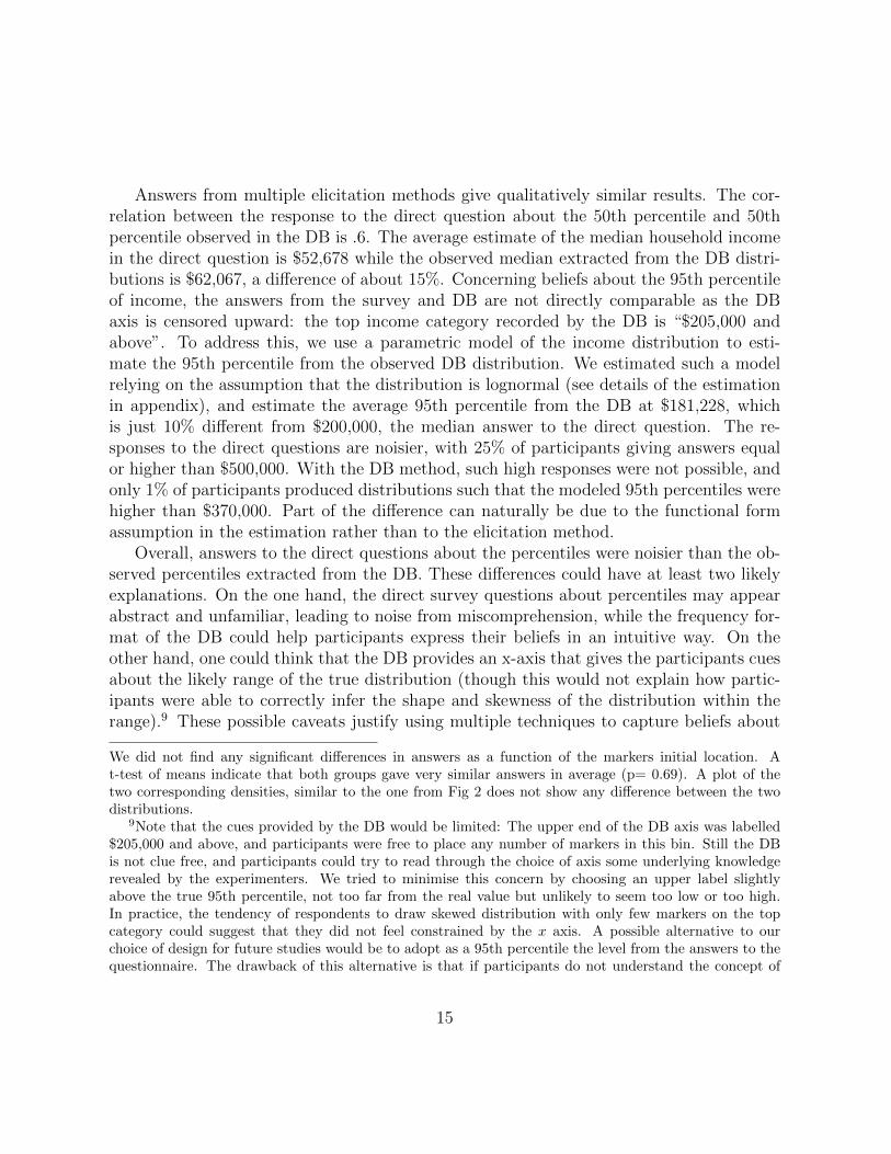
Answers from multiple elicitation methods give qualitatively similar results. The cor-relation between the response to the direct question about the 50th percentile and 50thpercentile observed in the DB is .6. The average estimate of the median household incomein the direct question is $52,678 while the observed median extracted from the DB distri-butions is $62,067, a difference of about 15%. Concerning beliefs about the 95th percentileof income, the answers from the survey and DB are not directly comparable as the DBaxis is censored upward: the top income category recorded by the DB is “$205,000 andabove”. To address this, we use a parametric model of the income distribution to esti-mate the 95th percentile from the observed DB distribution. We estimated such a modelrelying on the assumption that the distribution is lognormal (see details of the estimationin appendix), and estimate the average 95th percentile from the DB at $181,228, whichis just 10% different from $200,000, the median answer to the direct question. The re-sponses to the direct questions are noisier, with 25% of participants giving answers equalor higher than $500,000. With the DB method, such high responses were not possible, andonly 1% of participants produced distributions such that the modeled 95th percentiles werehigher than $370,000. Part of the difference can naturally be due to the functional formassumption in the estimation rather than to the elicitation method.
Overall, answers to the direct questions about the percentiles were noisier than the ob-served percentiles extracted from the DB. These differences could have at least two likelyexplanations. On the one hand, the direct survey questions about percentiles may appearabstract and unfamiliar, leading to noise from miscomprehension, while the frequency for-mat of the DB could help participants express their beliefs in an intuitive way. On theother hand, one could think that the DB provides an x-axis that gives the participants cuesabout the likely range of the true distribution (though this would not explain how partic-ipants were able to correctly infer the shape and skewness of the distribution within therange).9 These possible caveats justify using multiple techniques to capture beliefs about
We did not find any significant differences in answers as a function of the markers initial location. At-test of means indicate that both groups gave very similar answers in average (p= 0.69). A plot of thetwo corresponding densities, similar to the one from Fig 2 does not show any difference between the twodistributions.
9Note that the cues provided by the DB would be limited: The upper end of the DB axis was labelled$205,000 and above, and participants were free to place any number of markers in this bin. Still the DBis not clue free, and participants could try to read through the choice of axis some underlying knowledgerevealed by the experimenters. We tried to minimise this concern by choosing an upper label slightlyabove the true 95th percentile, not too far from the real value but unlikely to seem too low or too high.In practice, the tendency of respondents to draw skewed distribution with only few markers on the topcategory could suggest that they did not feel constrained by the x axis. A possible alternative to ourchoice of design for future studies would be to adopt as a 95th percentile the level from the answers to thequestionnaire. The drawback of this alternative is that if participants do not understand the concept of
15
income inequality, such as the items concerning the incomes of typical professions. Theseprofessional income questions also have the advantage of being more concrete than the DBtask. Figure 3 shows the distribution of beliefs for the four professions. It is interestingto observe that the answers to these questions also indicate a tendency to underestimateinequalities. Using Bureau of Labor Statistics data to approximate the values of the an-swer to the questions, we find that more than 70% of the participants provided incomes forchairpeople below the actual average income for chairpeople.10 Furthermore, a majority ofparticipants overestimated the income of skilled and unskilled workers, with 82% and 84%of participants providing incomes higher than the average income of these groups. The dataalso show a significant dispersion of answers expressing the imprecision of the participants’level of knowledge about what various workers earn.
The results of the varied elicitation methods suggest that even though each methodmay present some limitations, their use in conjunction allows for a better understanding ofindividuals’ beliefs about the income distribution.
4.1.2 Participants’ individual characteristics and subjective beliefs
To assess whether differences in subjective beliefs are associated with differences in individ-ual characteristics, we use OLS regressions to look at the correlations between the subjectivebeliefs about the income distribution and participants’ characteristics. While we find thatseveral characteristics are correlated with beliefs, we find only limited correlations betweenbeliefs and local economic variables.
We use the estimates from the DB to look at the individual differences in beliefs aboutpercentiles (namely the 10th, 25th, 50th, 75th, and 90th percentiles) of the income distri-bution. In Table 2, columns 1–6 show the results of OLS regressions with these variablesas explained variables. As a measure of income dispersion, we use the interquartile range(column 7) and we also use the two direct questions from the survey about the 50th and95th percentiles. We find that older and more educated people tend to give a more accurate
95th percentile, it can introduce noise in the elicitation procedure by creating an upper income categorywhich is way off the mark.
10We took the data from the of labor statistics (2010). While our survey questions asked for averageincome, the BLS only give data for median income. This is likely to give a lower bound for the averageincome in the profession, in particular for doctors and chairpeople where a negative skew in the distributionis likely to exist. For each category, we took a representative profession listed by the BLS (overall resultsare not sensitive to the choice of other specific professions. The BLS data gives: 1) Unskilled factory worker(Food processing workers) $23, 000 per year 2) Skilled factory workers (Industrial Machinery Mechanicsand Maintenance Workers) $44, 000 per year 3) Doctors (Physicians and Surgeons) $166, 400 per year 4)Chairman of a large national corporation (based on 158 Standard & Poors 500 index companies) $9, 000, 000per year
16
picture of the income distribution with lower income estimates for lower percentiles andhigher income estimates for higher percentiles. As a consequence, the distribution of theinterquartile range for older and more educated people is more concentrated around theactual value. Personal income correlates positively with the beliefs about the level of almostall percentiles except the highest ones. Our results suggest that wealthier participants tendto overestimate the income of the bottom 90% of the population.
Most local variables, such as local income inequality, are not correlated with beliefselicited with the DB.11 This stands in contrast to recent studies finding that local situationsaffect perceptions of global conditions (Snowberg, Meredith, and Ansolabehere 2011, Li,Johnson, and Zaval 2011, Cruces, Perez Truglia, and Tetaz 2013). The estimated numberof African Americans in a ZIP code does correlate with beliefs about income inequalities,with people living in areas with more African Americans being less likely to overestimatethe lowest percentiles of the income distribution.12
Once again, the results from the multiple elicitation methods lend support for the useof the DB. When comparing the regression results using answers about the 50th percentilesfrom the DB and from the direct questions, the results are reasonably close (see Table 2).Looking at the correlation between participants’ characteristics and their beliefs about thetypical level of income of the four specific professions gives results that are largely in linewith those collected with the DB (see Table 3). More educated participants made moreaccurate inferences about the average income of professions, providing lower estimates forskilled and unskilled workers and higher estimates for chairpeople. Participants with higherincomes overestimated the incomes of unskilled and skilled workers. Older respondentstended to give higher estimates for each profession instead of giving lower estimates forlow income professions and higher estimates for high income professions. The inclusionof local variables in these regressions shows that in areas where the average income perhousehold is higher, participants tended to have lower estimates of the yearly income ofunskilled and skilled workers and tended to provide higher estimates of a chairperson’syearly income. It is not clear a priori whether this reflects an effect of the local incomedistribution. A reference-group approach (Cruces, Perez Truglia, and Tetaz 2013) wouldon the contrary suggest that people living in richer neighborhoods overestimate the incomeof poorer households in the country. It is possible that this effect only reflects betterknowledge of the distribution by households living in richer neighborhoods–note that the
11In addition, we also tested for possible correlations between more elaborate measures of inequality,such as the Gini coefficient, between the DB distribution and the local distribution of income at the Ziplevel or in the county (using both income standard deviation and local Gini coefficients). We did not findany correlation.
12Our sample does not contain enough African American or Asian American participants to estimatesignificant differences between these categories and White Americans in terms of beliefs.
17
signs of the coefficients follow the same patterns as for the education variable.
18
(1)
(2)
(3)
(4)
(5)
(6)
(7)
(8)
(9)
10th
25th
50th
75th
90th
95th
50th
95th
Percentile
Percentile
Percentile
Percentile
Percentile
Percentile
Interquartile
Percentile
Q.
Percentile
Q.
Educa
tion
-1916.92**
-1611.10*
-2797.30**
-3436.17*
-1425.47
1997.46
-0.04
-2746.96**
8.32e+
07
(680.69)
(779.15)
(966.83)
(1394.08)
(1725.78)
(1764.24)
(0.04)
(1016.69)
(6.60e+
07)
Inco
me
0.03***
0.04***
0.06***
0.07***
0.07**
0.04
-0.00
0.05***
-613.59
(0.01)
(0.01)
(0.01)
(0.02)
(0.02)
(0.03)
(0.00)
(0.01)
(479.66)
Male
75.23
-687.19
-1771.05
-2582.94
-2164.78
-1618.98
-0.04
-4623.94**
9.66e+
07
(1121.90)
(1219.15)
(1540.45)
(2208.14)
(2740.66)
(2856.19)
(0.06)
(1519.81)
(1.29e+
08)
Age
-143.00***
-84.16*
77.94
367.14***
612.41***
667.70***
0.01***
-80.16
2.09e+
06
(34.91)
(41.30)
(55.56)
(76.99)
(97.15)
(100.06)
(0.00)
(55.24)
(1.44e+
06)
Loca
lpop.den
s.51955.37
82759.45
99530.00
175841.14
136886.77
403052.11
5.79
47742.43
-9.11e+
09
(208316.26)
(219480.23)
(246939.62)
(259634.41)
(266338.12)
(266634.19)
(6.36)
(202819.61)
(7.70e+
09)
Loca
lavg.inc.
21.22
14.06
-18.13
-75.44
-85.45
-53.83
-0.00
-37.88
2.72e+
06
(29.62)
(32.83)
(41.15)
(59.61)
(74.51)
(80.53)
(0.00)
(44.09)
(3.54e+
06)
Loca
lst.dev
.inc.
0.02
0.07
0.10
0.07
0.17
0.25
0.00
0.13
123.35
(0.09)
(0.10)
(0.13)
(0.19)
(0.24)
(0.26)
(0.00)
(0.15)
(2271.35)
Loca
lBlack
pop.
-0.16*
-0.18*
-0.11
-0.03
0.30
0.43
0.00
-0.17
9790.70
(0.07)
(0.08)
(0.12)
(0.18)
(0.24)
(0.24)
(0.00)
(0.14)
(10084.31)
Loca
lAsianpop.
0.14
0.26
0.38
0.55
0.87
0.55
-0.00
0.19
12587.45
(0.21)
(0.20)
(0.23)
(0.38)
(0.59)
(0.55)
(0.00)
(0.29)
(13277.84)
Constant
39087.33***
47056.44***
59917.51***
79771.11***
96192.39***
104404.27***
1.80***
59898.00***
-4.29e+
08
(3963.03)
(4371.96)
(5911.59)
(8472.48)
(10930.51)
(11250.73)
(0.22)
(6287.20)
(4.15e+
08)
R-squared
0.04
0.02
0.02
0.04
0.05
0.06
0.03
0.02
-0.00
N825
825
825
825
825
825
825
825
825
*p<0.05,**p<0.01,***p<0.001
Tab
le2:
Bel
iefs
abou
tth
esh
ape
ofth
ein
com
edis
trib
uti
on.
The
dep
enden
tva
riab
les
are
atth
eto
pof
each
colu
mn.
Col
um
ns
(1)
to(7
)use
the
answ
ers
from
the
DB
,co
lum
ns
(8)
and
(9)
use
the
answ
ers
toth
esu
rvey
ques
tion
nai
re.
SE
inbra
cket
s.
19
(1) (2) (3) (4) (5) (6) (7) (8)Unskilled Unskilled Skilled Skilled Doctor Doctor Chairman Chairman
Table 3: Beliefs about the income level of typical professions. The dependent variables areat the top of each column. SE in brackets.
Overall, our results are globally consistent and do not indicate any major misalignmentbetween questions and answers across the DB and the survey questions. One limitation ofthe above approach is that it only allows studying the link between individual character-istics and specific parts of the distribution or specific statistics of dispersion. This can bemisleading as there can be a link between statistics of centrality and dispersion. This is thecase in particular for skewed distributions such as the income distribution. To address thisissue, we use maximum likelihood estimation of the parameters of a lognormal distributionthat best fits the distributions participants submitted with the DB. We can then estimatejointly the measures of centrality µ and dispersion σ for each participant’s DB distributionand can then model these two parameters as a function of individuals’ characteristics. Theresults of this estimation (provided in the appendix) provide qualitatively similar resultsto those of Table 2.
4.2 Beliefs about social mobility
4.2.1 Overall
Relative to previous studies looking at beliefs about income inequality, we asked questionsabout beliefs about social mobility, both in terms of personal prospects and in terms ofbeliefs about the possibility of social mobility in the USA. These different questions allowus to look at the predictions from the perspective of different economic theories regarding
20
the links between these measures and political positions.First, we measured the respondents’ beliefs about their own social mobility both in
terms of past mobility and in terms of prospects of future mobility. In regard to their pastmobility, respondents indicated a positive appraisal of their success. Asked whether theirposition and prospects in life are better than those of their parents, 81.1% answered either“slightly agree” or “strongly agree” with 30.6% of respondents strongly agreeing. Whenasked about their future mobility, through a question about their expectations of theirfuture household income in 5 years, respondents indicated an overall positive expectationof change with an average increase of $22,050 (median $10,000) with 90% of respondentsindicating variations between -$15,000 and +$45,000.
Second, respondents were asked about their general beliefs in social mobility in the USAand its causes. Overall, answers indicated positive beliefs about social mobility. On theopen society question, 81.4% of respondents answered from “slightly agree” to “stronglyagree”, with 20.3% strongly agreeing on the assertion that the USA is an open society. Inregard to the factor explaining success, only 7% of respondents declared that luck is themain determinant of success, 48.5% declared that both luck and hard work matter and44% indicated that hard work is the “most important”.
4.2.2 Participants’ individual characteristics and subjective beliefs
As with subjective beliefs about the income distribution, we can use the respondents’answers to assess how beliefs about social mobility vary between individuals with differentcharacteristics. Moreover, given that we jointly elicit beliefs about social mobility in generaland about participants’ own social mobility, we can study whether there is a link betweenthe two. Piketty (1995) proposes a model of learning in which participants’ beliefs aboutthe degree of social mobility in society is largely determined by their own experience. Asa consequence, perceptions about the overall level of social mobility should be positivelycorrelated with perceptions of personal upward mobility. This is indeed what we find.
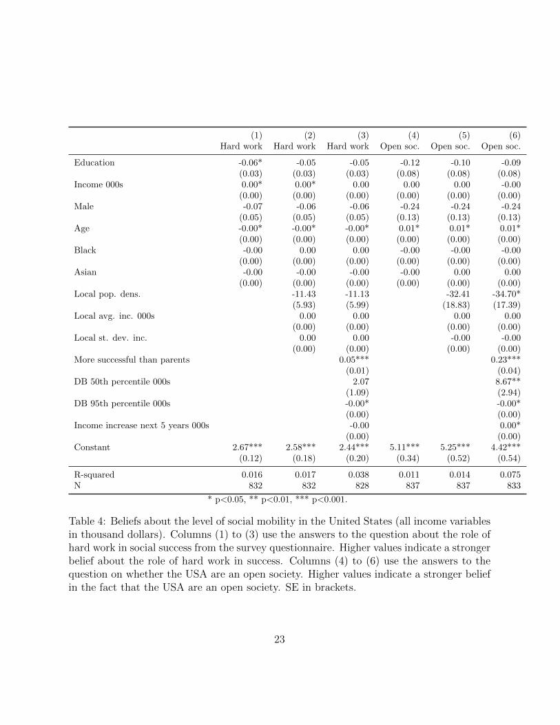
The results of regressions of the answers on the “hard work vs luck” question and on the“open society” question on the same variables as in Tables 2 and 3 are displayed in Table413 We also add variables reflecting beliefs about participants’ own social mobility at thepresent time (relative to their parents) and in the near future (expected change in incomeover the next five years). Furthermore, we include the estimated 50th and 95th percentilesfrom participants’ DB distributions to control for any correlation between shape of thesubjective distribution and beliefs about the procedural fairness leading to it. Columns1–3 show the answer to the question on hard work versus luck as the main determinant
13For this table and later tables some variables are categorical. We use OLS as a robust estimator.
21
of economic success (higher values indicate a stronger belief in the role of hard work).Columns 4–6 show the answers to the question on the open society (higher values indicatestronger belief in the openness of the American society).
With respect to demographics, age is the variable with the most consistent effect acrossdifferent sets of controls. Older participants are more likely to say that hard work is lessimportant than luck but at the same time, more likely to say that America has an opensociety where one’s success is not primarily determined by family background. We donot find that local situations predict respondents’ beliefs about equality of opportunity orsocial mobility. In terms of beliefs about the income distribution, the estimated percentileshave opposite but quite intuitive links with beliefs: a belief in a higher median income ispositively correlated with the belief in an open society, while a belief in a higher level ofincome for the top 5% of households is associated with a lower belief in social mobility (forboth items assessing it).
When introducing beliefs about participants’ own social mobility and about the incomedistribution, experienced social mobility by the participants becomes the strongest predic-tor of beliefs about equality of opportunity. Participants who declare that their currentposition and prospects are better than those which their parents faced at the same age aremuch more likely to believe in the existence of equality of opportunity. Noticeably, whenthe variable relating to doing better than one’s parents is introduced, the income variableloses significance. Overall, the importance of this variable is clearly compatible with thelearning model proposed by Piketty (1995). Beliefs about how one’s future income willincrease are slightly correlated with belief in an open society.
22
(1) (2) (3) (4) (5) (6)Hard work Hard work Hard work Open soc. Open soc. Open soc.
Table 4: Beliefs about the level of social mobility in the United States (all income variablesin thousand dollars). Columns (1) to (3) use the answers to the question about the role ofhard work in social success from the survey questionnaire. Higher values indicate a strongerbelief about the role of hard work in success. Columns (4) to (6) use the answers to thequestion on whether the USA are an open society. Higher values indicate a stronger beliefin the fact that the USA are an open society. SE in brackets.
23
5 Beliefs about income inequalities and political po-
sition
The large range of beliefs elicited (e.g., beliefs about the overall level of inequality, beliefin social mobility in general, personal experience of social mobility) allow us to study howthese different beliefs relate to political positions. To do so, we use beliefs to predict answersto two questions: a question on the preference for income redistribution, and a questionabout positioning oneself on a traditional left-right scale.
5.1 Preferences for redistribution
To study preferences for redistribution, we look at the question asking respondents whetherthey think that income differences are currently too large in America. Different theoriesmake distinct predictions about the link between beliefs about inequality and preferencesfor redistribution. First, the “inequality aversion” hypothesis, or the idea that peoplehave preferences for the level of inequality itself (Fehr and Schmidt 1999, Bolton andOckenfels 2000), predicts that the elicited beliefs about the level of income inequalitywould be the main predictors of redistribution preferences. Second, the social mobilityhypothesis (Piketty 1995, Benabou and Tirole 2006), or the reciprocity explanation (Fong,Bowles, and Gintis 2006) would suggest that the belief in an open society, hard work, andone’s personal experience of upward mobility would foster stronger preferences for redis-tribution. Finally, the idea that one’s prospect of upward mobility shapes redistributionpreferences (Hirschman and Rothschild 1973, Benabou and Ok 2001) would suggest that arespondent’s belief in the evolution of his or her income in the near future should matter.
Table 5 shows the regression results of the answers to this question on the characteristicsand beliefs of the participants. The first four columns control for beliefs about inequalityusing the DB data while the last four columns use the items about professions’ incomes.With regard to individual demographics, the results are in line with common patterns inwhich participants with higher incomes are significantly less favorable to redistributionwhile participants with higher levels of education and those from urban areas are morefavorable to it. When looking at the beliefs about income inequality, we find that thebeliefs about the level of inequality measured with an overall index of dispersion (here theinterquartile range14 from the DB) is significantly correlated with redistribution preferences(columns 1–3). Respondents who believe that the level of inequality in the US is relativelyhigh tend to be more favorable to redistribution.
14The results are robust to other specifications.
24
However, the significance of this effect disappears when controlling for beliefs aboutsocial mobility (column 4). Interestingly, when we use the items about the incomes ofspecific professions as a way to measure beliefs about income dispersion, we find that thebelief about the lowest income profession (unskilled worker in a factory) is always stronglysignificant: Participants are more likely to be in favor of income redistribution when theybelieve that unskilled workers in a factory have lower incomes (p<0.001). This suggeststhat redistribution preferences may be more sensitive to beliefs about the lower tail of theincome distribution. We investigate this possibility further below.
The prospect of upward mobility, measured by expectations of an income increase overthe next five years, is not significant at conventional level. It is near 5% in models (3)and (7), however, when we control for beliefs about social mobility in society (models(4) and (8)), the p-value climbs above 10%. Social mobility already experienced (i.e.,the question about present success relative to one’s parents) is not significantly correlatedwith preferences for redistribution when controlling for individuals characteristics. On thecontrary, we find that the beliefs about social mobility in general (questions about the USbeing an open society and whether hard work or luck is an explanation for social success)are the main predictors of preferences for redistribution. The significance of these beliefsas predictors is very strong (p<0.001) even when controlling for individual characteristics,individual experience, and personal prospects of social mobility.
Overall, our results lend support to social mobility or reciprocity explanations, andsuggest that the personal prospects of upward mobility are unlikely to be the main drivers ofredistribution preferences. In regard to the possible existence of an “aversion to inequality”,our results suggest that respondents are not so much averse to inequality or dispersionin general–as would be suggested by certain behavioral models (Fehr and Schmidt 1999,Bolton and Ockenfels 2000)–as they are to low incomes for the poorest members of thesociety, consistent with quasi-maximin preferences and a concave altruistic utility function(Charness and Rabin 2002, Andreoni and Miller 2002, Cox and Sadiraj 2006).15
15A possible concern could be that low income respondents are more knowlegeable about the income oflow income households than high income respondents who may overestimate the income from the pooresthouseholds in society. Such a situation would create the observed correlation if low income respondentstend to be in favour of redistribution and high income respondents tend to be against redistribution. Thefact that the coefficient on the belief about unskilled workers’ income does not change between column(5) and column (6) when the income of the respondent is included as a covariate tends to suggest that itis not what is driving the results. The coefficient from the income variable should partially capture thecorrelation between income and political position in column (6). The link between participants income andpolitical position could however be non linear and be imperfectly captured by the inclusion of the incomevariable in the regression. We therefore constructed a set of four dummies for the quartiles of the incomedistribution and we included them in the regression. The results show that the coefficients and their levelof significance are almost unchanged. This suggest that for respondents of different income levels, estimates
25
(1) (2) (3) (4) (5) (6) (7) (8)
Median DB 000s -0.00 -0.00 -0.00(0.00) (0.00) (0.00)
Interquantile range 0.07* 0.06* 0.04(0.03) (0.03) (0.03)
Income 000s -0.00** -0.00* -0.00** -0.00*(0.00) (0.00) (0.00) (0.00)
Male -0.11 -0.14 -0.10 -0.13(0.10) (0.10) (0.10) (0.10)
Age 0.00 0.00 0.01 0.00(0.00) (0.00) (0.00) (0.00)
Table 5: Regression of the tendency to be in favor of income redistribution (all incomevariables in thousands of dollars). SE in brackets.
5.2 Political positions
Political position was measured with a Likert scale item (henceforth, the “rightwing” vari-able) in which higher values indicate a tendency of be on the political right wing. Sim-ilar results to those we report below are obtained when looking at partisanship for theDemocrats or Republicans. We use the answers to this question to reproduce the sameregressions as in Table 5 with the political position variable as explained variable instead ofthe preference for redistribution. In this way, we can see whether the variables associatedwith a preference for less redistribution differ from those associated with a more right-wing
of income of unskilled workers is positively correlated with being against redistribution.
26
position.The results of regressions of the “rightwing” variable on beliefs about the income dis-
tribution are displayed in Table 6. As in the previous table, we do not find a significanteffect of the perceived shape of the income distribution (median, interquartile range) whenbeliefs about social mobility are controlled for. Overall, when controlling for participants’beliefs about social mobility, the only individual characteristics which remain significant areeducation and urban location. The household income variable loses significance. Partici-pants who exhibit upward mobility themselves are significantly more likely to be rightwing.However, when beliefs about social mobility in society are controlled for, this correlationvanishes. This result is in agreement with Piketty’s (1995) model of rational learning inwhich individuals use their own social mobility to infer the degree of social mobility insociety which, in turn, determines their position for more or less redistribution.16 Thecoefficients of the prospect of upward mobility over the next five years are not significant.
Here again we find that beliefs about the average income of unskilled workers are cor-related with political positions. Higher estimates of unskilled factory workers income arepositively associated with right-wing leanings. We also find that, to a lower degree, this isalso true for estimates of doctors’ incomes.
To compare the relative effect of each variable we use the model (8) and comparethe effect–on the right-wing variable–of one standard deviation in the different explainingvariables with a significant coefficient. The variables with the largest effect (above 10% ofstandard deviation) are views about the role of hard work (0.31), the existence of an opensociety (0.20), the estimated income of an unskilled factory worker (0.26), the educationlevel of the participant (-0.25) and the population density (-0.23). The effects of therespondents’ own income (0.11) and the estimated income of doctors (0.09) have relativelya lower magnitude.
Overall, these results suggest that beliefs about inequality do play a significant rolein determining political positions. However, they indicate that the effects seem to bedriven by the beliefs about equality of opportunity and beliefs about the incomes of thepoorest households in society. To further investigate the role of beliefs about the pooresthouseholds in society, we use the rich information elicited with the DB. Instead of onlyextracting the median in the distribution, we extract a wider range of percentiles in thesubjective distributions. This allows us to study whether various parts of the subjectivedistributions are more correlated with political positions than others. If a left-wing positionis linked with the view that inequality is too great, this could be driven either by a concernfor the poorest households, or by a reprobation for the incomes of the richest people, or by
16The coefficients moved in the same direction in the regression on the question asking whether incomedifferences in America are too large, but the coefficients were not significant.
27
(1) (2) (3) (4) (5) (6) (7) (8)
Median DB 0.01* 0.01 0.00(0.00) (0.00) (0.00)
Interquantile range 0.01 -0.01 0.02(0.05) (0.06) (0.06)
Income 000s 0.00* 0.00 0.00* 0.00(0.00) (0.00) (0.00) (0.00)
Male 0.15 0.21 0.11 0.18(0.13) (0.13) (0.13) (0.13)
Age 0.01* 0.01* 0.01 0.01(0.00) (0.00) (0.00) (0.00)
Table 6: Regression of the tendency to be rightwing (all income variables in thousands ofdollars). SE in brackets.
both. In Table 7, we show the results of replacing the median in models (1), (2) and (4) bykey percentiles. The coefficients for each percentile are displayed for the three regressionmodels. The results confirm those from Tables 5 and 6, namely, that the beliefs aboutthe income of the poorest households in the society are those which correlate most highlywith political positions. Providing high estimates of the poorest people’s income predictsbeing on the right, while beliefs about the income of wealthier groups do not correlate withpolitical positions. This pattern persists and stays significant even when covariates frommodels (2) and (4) of Table 6 are included in the regression. These results bring supportto those from Table 5 and Table 6 where the beliefs about unskilled workers income havea strong and very significant effect on preferences for redistribution an political positions,
28
respectively. One possible explanation could be that higher income respondents are bothless informed about low household incomes (and as a consequence overestimated them)and more conservatives. In that case, the correlation between beliefs and political positionwould just be a spurious link created by the correlation between the political position ofthe respondent and his/her degree of error made when asked to guess the level of income ofthe poorest households. We checked for such a possible explanation by running the sameregression on the subsample of respondents with an income lower than $50,000 (median ofthe US distribution of household incomes) and on the subsample of those whose income ishigher than $80,000 (75th percentile of the distribution) poorest respondents in our sample.In both samples, beliefs about the income of the poorest had a similarly positive marginaleffect on political positions. This indicates that the observed correlation between beliefsabout the lowest incomes in society and political positions is not reflecting different errorsfrom respondents.
Overall, our results suggest that, while political positions are not very sensitive to thecentrality and dispersion of the perceived income distribution, they are influenced by beliefsabout the incomes of the poorest. This result stands in contrast to views in which self-interest or a philosophical objection to inequality largely governs redistribution preferences.Interestingly, our results with the DB indicate that the beliefs about the top 5th percentileof the distribution are not correlated with political position. A limit of the DB is that ithas an upper bound at $205,000. The answers from the survey about a chairman incomeseemed to back this lack of correlation between beliefs about high income and politicalposition. The beliefs about doctors’ income do not respect this pattern. Even though thisresult is less robust and significant than the link observed for unskilled workers’ income, itmay suggest that more research is warranted about beliefs about high incomes.17
17We checked here again that this result could not simply reflect a better information from higher incomerespondents who tend to be more conservative. The magnitude of the coefficient does not decrease whenthe regressions are made within samples of richer and poorer respondents.
29
Table 7: Beliefs on different percentile of the distribution of income and rightwing position
Percentile 5 10 25 50 75 90 95
No control (1) 0.15∗∗ 0.15∗∗ 0.12∗∗ 0.08∗ 0.04† 0.02 -0.00Demographics controls (2) 0.13∗∗ 0.13∗ 0.11∗∗ 0.06† 0.03 0.01 0.00Demographic and beliefs controls (4) 0.13∗ 0.13∗ 0.11∗ 0.06† 0.03 0.01 0.00
For an increase of $10,000 in the perceived income percentile from the DB (in column), each number in the
table represents the marginal effect on the variable indicating a right wing position. The first column
represents the marginal x represents increase of $10,000 in the 5th percentile, and so on. These coefficients
are estimated by the OLS regressions from Table 6 median in columns (1), (2) and (3). The coefficients for the
percentile 50 are the same as those for the median in the Table 6. Coefficients significant at † 10%, ∗ 5%, ∗∗ 1%.
6 Discussion
The political economy and political science literatures have suggested several potential linksbetween income inequality and preferences for wealth redistribution. In this work, we haveelicited subjective beliefs about several dimensions of income inequality and investigatedboth the possible factors influencing these beliefs as well as the role these beliefs may playin determining political positions.
First, in contrast to recent studies finding evidence that local variables influence indi-vidual’s beliefs about the state of the economy nationally, we find only limited evidencethat beliefs about the national income distribution are influenced by the characteristics ofthe local income distribution (such as local average income or income dispersion). How-ever, we do find that wealthier people assume that incomes are higher (their subjectivedistributions are shifted to the right) suggesting a kind of hyper-local influence on sub-jective estimates: neighbors’ incomes do not seem to affect one’s impressions, but one’sown income does. This result is somewhat different than that of Cruces, Perez Truglia,and Tetaz (2013), which suggests that the relative position in the local income distributioninfluences a household’s beliefs in its relative position in the national income distribution.Several reasons could explain these differences such as the different countries where thestudies take place (USA and Argentina) or the different set of controls used in each study(we controlled for a wide range of local characteristics). One of the possible limitations ofour strategy to study the role of local variables is that we may have failed to identify theright level of “locality” by using the characteristics of the ZIP code area. In that sense,our lack of results with local variables should not be seen as proof that local variables donot matter. Further studies could investigate other levels of geographical locality as well
30
as the role of “local” information provided by social networks (friends, workplace).18
Second, we looked at the possible role of these beliefs in shaping preferences for redis-tribution. We find that beliefs about the income distribution are correlated with individualpreferences for redistribution. Interestingly, we do not find any effect of the standardstatistics of centrality or variance of the distribution. The main link between the perceivedincome distribution and political position on a left-right axis is the belief about incomeof the poorest members of society. We find that higher estimates of the incomes of thepoorest (whether directly stated or extracted from the lower percentiles of people’s DB ren-dering of the income distribution) are strongly correlated with a right-wing political leaning.Notably, this specific link between beliefs about the income distribution and political pref-erences is not what would naturally stem from the models of inequality aversion (Fehr andSchmidt 1999, Bolton and Ockenfels 2000) which suggest a rejection of distributions withlarger inequality. On the other hand, this result is in line with quasi-maximin and concavealtruistic utility preferences in which individuals’ utility over income distributions includesa trade off between efficiency and the conditions of those who are the worst off (Charnessand Rabin 2002, Andreoni and Miller 2002, Cox and Sadiraj 2006). Such preferences areclose to Rawls’ maximin preferences (Rawls 1971), in which people care primarily aboutensuring the highest level of resources for the poorest members of society.19
In addition to beliefs about inequalities, we find favorable support for the theory thata belief in the existence of social mobility may determine attitudes towards redistribution(Piketty 1995, Alesina and Angeletos 2005, Benabou and Tirole 2006). Previous empiricalstudies have used survey data to provide support to this idea (Piketty 1996, Corneo andGruner 2002). The present study provides further evidence by estimating the correlationbetween these beliefs and preference for redistribution while controlling for a wider rangeof beliefs about income inequality. Not only does this approach test the robustness of paststudies, it also permits for the testing of more theories than was possible with existingsurveys. In particular, we tested the joint role of beliefs about inequality and respondents’prospects of upward mobility (Hirschman and Rothschild 1973, Ravallion and Lokshin 2000,Benabou and Ok 2001, Fillippin and Checchi 2004). While a belief in social mobility ingeneral predicts political positions, it is not the case for one’s own personal chances ofupward mobility.
In the television program The West Wing, the U.S. President is asked “Who gives a
18We also investigated the effect of inequalities at the county level, with the same limited results. Ifanother level of locality is appropriate, we suspect it may be a level closer to the respondent.
19The recent “Occupy Wall Street” political movement, rallying under the cry of “We are the 99%”, usedthe high level of inequality at the top of the income distribution to mobilize support. Our results suggestthat people may be more influenced towards redistribution by focusing on the lower end of the distributioninstead.
31
damn, sir? This is a tax cut that benefits only 4,500 families.” The President replies, “Itdoesn’t matter if most voters don’t benefit. They all believe that someday they will. That’sthe problem with the American dream: it makes everyone concerned for the day they’regonna be rich.” In contrast to this opinion, which suggests that voters are concerned forthe day they will become rich, the present investigation finds empirical support for the ideathat people oppose further redistribution when they believe that anyone can become rich.
A Appendix: Survey sample
The Table below compares the sampling firm panel demographics to our sample. Thelargest differences is observed for gender with more female respondents than in the overallpanel. We have already experienced such a gender imbalance in previous uses of this firmpanel. This suggests that it may be due to a general gender differences in the propensityto participate to a survey rather than a selection induced specifically by our topic. We alsoobserve a smaller number of young participants, a larger number of participants with highincome. We have now added this information to the description of our sample.
We retained 82% of the initial sample and eliminated respondent who looked that theymay not have taken the task seriously. Table 9 compares the answers of both samples(retained and not retained). On most answers, there are no significant differences. Thestandard deviation of the distribution elicited by the DB is significantly higher in theretained sample relative to the non retained sample. It is likely to be a mechanical effectof the rule we chose: we eliminated participants who clicked less than 5 times on the DB.This is likely to eliminate participants who created DB distributions with only limiteddispersion. The retained sample also display a belief which is (marginally) significantlyhigher than for the non retained sample. Overall, our choice to retain the sample do notlead to a sample of respondents with very different answers. In particular, there are nosignificant differences in regard to the answers to the political questions.
Table 8: Comparison of the study sample with the sampling firm panel demographics
Retained sample Non retained sample t-test p-value
Mean DB 72,749 73,205 0.78Median DB 52,938 51,117 0.30St. Dev. DB 39,925 32,428 <0.001*Income chairman 1,031,365 889,892 0.02*Income doctor 258,879 258,753 0.99Income skilled w. 60,369 56,478 0.05*Income unsk. w. 32,872 31,263 0.11Open Society 5.23 5.15 0.54Hard work 2.36 2.40 0.47Parent 5.35 5.42 0.33Right wing 3.83 3.64 0.18Democrat 57.6% 58.3% 0.88N 839 186
Table 9: Comparison of the retained sample with the non retained sample
33
B Appendix: Structural estimation
Estimating a parametric distribution from DB data requires taking into account that theDB allows participants to give an estimate of the percentage of households in a series ofbrackets 10,000 dollars wide each, up to the highest bracket “$205k and above”. To sum-marize beliefs about the income dispersion in one parameter, we model the DB observationsas coming from a lognormal distribution with mean and standard deviation µ and σ. Toestimate these parameters for each participant, we maximise the log-likelihood function foreach individual i:
`(µi, σi|Mi) =100∑k=1
22∑j=1
ln
(Φ
(ln(bj)− µi
σi
)− Φ
(ln(bj)− µi
σi
))1{mki∈[bj ,bj ]}
Where Mi is the vector of observed marker values mki for the individual i, with k beingthe id of the marker for each participant, j the id of the bracket and bj, bj respectively the
lower and upper bounds of bracket j (with b1 = 0 and b22 = +∞).This model allows us to estimate how different participant characteristics correlate with
participants’ beliefs about the shape of the distribution. To do so, we sum the individuallog likelihood over the whole sample:
L(µ, σ|M) =N∑i=1
`(µi, σi|Mi) (5)
Where M is the vector of all observed marker values mki in the sample. In order toestimate links between individual and local characteristics of participants and their beliefs,we parametrize the coefficients as linear functions of vectors of observed variables X1 andX2 respectively:
µ = β1X1
σ = β2X2(6)
Table 10 shows the results of the estimations of parameters µ and σ from the lognormaldistribution by maximizing the likelihood (5). The parameters are written as linear func-tions of variables characterizing the individual and local characteristics following equation(6). To take the non-independence of observations within participants into account, we usea robust matrix of variance clustered by participants. We find that education and age aresignificant, while no local variable is significant.
Table 10: Beliefs about the moments of the distribution from the distribution builder
35
C Appendix: median comparison
An interesting feature of our design is the elicitation of the subjectif belief about the medianhousehold income using two different methods: a direct question and the DistributionBuilder. Figure 4 shows the scatterplot of the individual answers to these two methods.There are clearly lots of variations accross the two elicitation methods reflected in theoverall correlation of 0.6 between the two types of answers. We think that these differencecan be due to the abstract nature of the direct question which require participants to thinkabout the notion of percentile. This may lead to more noisy answer from guesses. Anotherpossibility is that people may take more or less care in answering each question. Overall60% of participants’s estimates about the median via these two methods are within $10,000from each other and 78% are within $20,000.
36
Figure 4: Individual answers about the median in the questionnaire and in the DB
References
Alesina, A., and G. Angeletos (2005): “Fairness and redistribution,” The AmericanEconomic Review, 95(4), 960–980.
Alesina, A., and P. Giuliano (2009): “Preferences for redistribution,” Discussion pa-per, National Bureau of Economic Research.
Alesina, A., and E. La Ferrara (2005): “Preferences for Redistribution in the Landof Opportunities,” Journal of Public Economics, 89(5-6), 897–931.
Amiel, Y., F. Cowell, and W. Gaertner (2009): “To be or not to be involved:a questionnaire-experimental view on Harsanyis utilitarian ethics,” Social choice andwelfare, 32(2), 299–316.
Andreoni, J., and J. Miller (2002): “Giving According to GARP: An ExperimentalTest of the Consistency of Preferences for Altruism,” Econometrica, 70(2), 737–753.
Atkinson, A. (1970): “On the measurement of inequality,” Journal of economic theory,2(3), 244–263.
Atkinson, A., and F. Bourguignon (1982): “The comparison of multi-dimensioneddistributions of economic status,” The Review of Economic Studies, 49(2), 183–201.
37
Benabou, R. (2000): “Unequal societies: Income distribution and the social contract,”American Economic Review, pp. 96–129.
Benabou, R., and E. Ok (2001): “Social Mobility and the Demand for Redistribution:the POUM Hypothesis.,” The Quarterly Journal of Economics, 116(2), 447–487.
Benabou, R., and J. Tirole (2006): “Belief in a Just World and Redistributive Poli-tics*,” The Quarterly Journal of Economics, 121(2), 699–746.
Besley, T. (2007): “The New Political Economy*,” The Economic Journal, 117(524),F570–F587.
Bolton, G., and A. Ockenfels (2000): “ERC: A theory of equity, reciprocity, andcompetition,” American economic review, pp. 166–193.
Brunner, E., S. Ross, and E. Washington (2011): “Economics and Policy Prefer-ences: Causal Evidence of the Impact of Economic Conditions on Support for Redistri-bution and Other Ballot Proposals,” The Review of Economics and Statistics, 93(3).
Charness, G., and M. Rabin (2002): “Understanding social preferences with simpletests,” The Quarterly Journal of Economics, 117(3), 817.
Cleave, B. L., N. Nikiforakis, and R. Slonim (2010): “Is There Selection Bias inLaboratory Experiments?,” University of Sydney - Economics Working Paper Series.
Corneo, G., and H. Gruner (2002): “Individual preferences for political redistribu-tion,” Journal of Public Economics, 83(1), 83–107.
Cox, J., and V. Sadiraj (2006): “Direct tests of models of social preferences and a newmodel,” Andrew Young School of Policy Studies Research Paper Series, 07-13.
Cruces, G., R. Perez Truglia, and M. Tetaz (2013): “Biased perceptions of incomedistribution and preferences for redistribution: Evidence from a survey experiment,”Journal of Public Economics, 98, 100–112.
Di Tella, R., S. Galiani, and E. Schargrodsky (2007): “The formation of be-liefs: evidence from the allocation of land titles to squatters,” The Quarterly Journal ofEconomics, 122(1), 209.
Downs, A. (1957): An Economic Theory of Democracy. Harper, New York.
38
Engelmann, D., and M. Strobel (2004): “Inequality aversion, efficiency, and maximinpreferences in simple distribution experiments,” The American Economic Review, 94(4),857–869.
(2007): “Preferences over Income Distribution, Experimental Evidence,” PublicFinance Review, 35(2), 285–310.
Falk, A., E. Fehr, and U. Fischbacher (2008): “Testing theories of fairness–Intentions matter,” Games and Economic Behavior, 62(1), 287–303.
Fehr, E., and K. Schmidt (1999): “A Theory of Fairness, Competition, and Coopera-tion,” The Quarterly Journal of Economics, 114(3), 817–868.
Fillippin, A., and D. Checchi (2004): “An experimental study of the POUM hypoth-esis,” Research on economic inequality, 11.
Fong, C. (2001): “Social preferences, self-interest, and the demand for redistribution,”Journal of Public Economics, 82(2), 225–246.
Fong, C., S. Bowles, and H. Gintis (2006): “Strong reciprocity and the welfare state,”Handbook on the Economics of Giving, Reciprocity and Altruism, 2, 1439–1464.
Gigerenzer, G. (1991): “How to make cognitive illusions disappear: Beyond heuristicsand biases,” European review of social psychology, 2(1), 83–115.
Giuliano, P., and A. Spilimbergo (2009): “Growing up in a Recession: Beliefs andthe Macroeconomy,” Discussion paper, National Bureau of Economic Research.
Goldstein, D., E. Johnson, and W. Sharpe (2008): “Choosing Outcomes versusChoosing Products: Consumer-Focused Retirement Investment Advice,” Journal of Con-sumer Research, 35(3), 440–456.
Harrison, E., and C. Seidl (1994): “Perceptional inequality and preferential judge-ments: An empirical examination of distributional axioms,” Public Choice, 79(1), 61–81.
Harrison, G. W., M. I. Lau, and E. Elisabet Rutstrom (2009): “Risk attitudes,randomization to treatment, and self-selection into experiments,” Journal of EconomicBehavior & Organization, 70(3), 498–507.
Harsanyi, J. (1955): “Cardinal welfare, individualistic ethics, and interpersonal compar-isons of utility,” The Journal of Political Economy, pp. 309–321.
39
Harsanyi, J. (1975): “Can the maximin principle serve as a basis for morality? A critiqueof John Rawls’s theory,” The American Political Science Review, 69(2), 594–606.
Hirschman, A., and M. Rothschild (1973): “The changing tolerance for income in-equality in the course of economic development,” The Quarterly Journal of Economics,87(4), 544.
Karni, E., and Z. Safra (2002): “Individual sense of justice: a utility representation,”Econometrica, 70(1), 263–284.
Kitschelt, H. (1994): The transformation of European social democracy. CambridgeUniversity Press.
Kolm, S.-C. (1969): “The optimal production of social justice,” in Public economics, ed.by J. Margolis, and S. Guitton, pp. 145–200. Macmillan, London.
Kuziemko, I., M. Norton, E. Saez, and S. Stantcheva (2013): “How Elastic ArePreferences for Redistribution? Evidence from Randomized Survey Experiments,” Dis-cussion paper, National Bureau of Economic Research.
Li, Y., E. J. Johnson, and Zaval (2011): “Local Warming: Daily Temperature Devi-ation Affects Beliefs and Concern about Climate Change,” Psychological Science, 22(4),454–459.
Magee, L., A. Robb, and J. Burbidge (1998): “On the use of sampling weights whenestimating regression models with survey data,” Journal of Econometrics, 84(2), 251–271.
Meltzer, A., and S. Richard (1981): “A rational theory of the size of government,”The Journal of Political Economy, pp. 914–927.
Norton, M., and D. Ariely (2011): “Building a better Ameerica one wealth quintileat a time,” Perspectives on Psychological Science, 6(1), 9.
Nozick, R. (1974): Anarchy, state, and utopia, vol. 5038. Basic Books (AZ).
of labor statistics, B. (2010): “Occupational Outlook Handbook,” US Department ofLabor, Spring.
Persson, T., and G. Tabellini (2002): Political economics: explaining economic policy.MIT press.
40
Piketty, T. (1995): “Social mobility and redistributive politics,” The Quarterly Journalof Economics, 110(3), 551.
(1996): “Mobilite economique et attitudes politiques face a la redistribution,”CEPREMAP working document No 9603.
(2003): “Attitudes vis-a-vis des inegalites de revenu en France: existerait-il unconsensus,” Comprendre, 4, 209–41.
Poole, K., and H. Rosenthal (1991): “Patterns of congressional voting,” AmericanJournal of Political Science, pp. 228–278.
Przeworski, A., and J. Sprague (1986): Paper stones: A history of electoral socialism.University of Chicago Press Chicago.
Rabin, M. (1993): “Incorporating fairness into game theory and economics,” The Amer-ican Economic Review, pp. 1281–1302.
Ravallion, M., and M. Lokshin (2000): “Who wants to redistribute?:: The tunneleffect in 1990s Russia,” Journal of Public Economics, 76(1), 87–104.
Rawls, J. (1971): “A Theory of Justice (Cambridge,” Mass.: Harvard University.
Romer, T. (1975): “Individual welfare, majority voting, and the properties of a linearincome tax,” Journal of Public Economics, 4(2), 163–185.
Snowberg, E., M. Meredith, and S. Ansolabehere (2011): “Mecro-EconomicVoting: Local Information and Micro-Perceptions of the Macro-Economy,” SSRN:http://ssrn.com/abstract=1856286.
Surowiecki, J. (2004): “The Wisdom of Crowds: Why the Many Are Smarter Than theFew and How Collective Wisdom Shapes Business,” Economies, Societies and Nations.
Traub, S., C. Seidl, U. Schmidt, and M. Levati (2005): “Friedman, Harsanyi,Rawls, Boulding–or somebody else? An experimental investigation of distributive jus-tice,” Social Choice and Welfare, 24(2), 283–309.
Von Gaudecker, H.-M., A. Van Soest, and E. Wengstrom (2008): “Selection andmode effects in risk preference elicitation experiments,” IZA Discussion Paper.
Weymark, J. (1981): “Generalized Gini inequality indices,” Mathematical Social Sci-ences, 1(4), 409–430.