AALTO UNIVERSITY School of Science and Technology Faculty of Electronics, Communications and Automation Samppa Hyrkäs COMPARISON OF WIDEBAND EARPIECE INTEGRATIONS IN MOBILE PHONE Thesis for Master of Science degree has been submitted for approval on January 4 th 2010 in Espoo, Finland Supervisor Paavo Alku, Prof. Instructor Panu Nevala, MSc.
Transcript
AALTO UNIVERSITY
School of Science and Technology
Faculty of Electronics, Communications and Automation
Samppa Hyrkäs
COMPARISON OF WIDEBAND EARPIECE INTEGRATIONS IN
MOBILE PHONE
Thesis for Master of Science degree has been submitted for approval on January 4th
2010 in Espoo, Finland
Supervisor
Paavo Alku, Prof.
Instructor
Panu Nevala, MSc.
i
AALTO UNIVERSITY SCHOOL OF SCIENCE AND TECHNOLOGY
Abstract of the Master’s Thesis
Author: Samppa Hyrkäs
Name of the thesis: Comparison of Wideband Earpiece Integrations in Mobile
Phone
Date: 04.01.2010 Number of pages: 7 + 69
Department: Department of Signal Processing and Acoustics
Professorship: S-89, Acoustics and Audio Signal Processing
Supervisor: Professor Paavo Alku
Instructor: M.Sc.(Tech) Panu Nevala
The speech in telecommunication networks has been traditionally narrowband
ranging from 300 Hz to 3400 Hz. It can be expected that wideband speech call
services will increase their foothold in the markets during the coming years.
In this thesis speech coding basics with adaptive multirate wideband (AMR-WB)
are introduced. The wideband codec widens the speech band to new range from 50
Hz to 7000 Hz using 16 kHz sampling frequency. In practice the wider band means
improvements to speech intelligibility and makes it more natural and comfortable to
listen to.
The main focus of this thesis work is to compare two different wideband earpiece
integrations. The question is how much the end-user will benefit from using a larger
earpiece in a mobile phone? To find out speaker performance, objective
measurements in free field were done for the earpiece modules. Measurements were
performed also for the phone on head and torso simulator (HATS) by wiring the
earpieces directly to a power amplifier and with over the air on GSM and WCDMA
networks. The results of objective measurements showed differences between the
earpiece integrations especially on low frequencies in frequency response and
distortion.
Finally the subjective listening test is done for comparison to see if the end-user
notices the difference between smaller and larger earpiece integrations using
narrowband and wideband speech samples. Based on these subjective test results it
can be said that the user can differentiate between two different integrations and that
a male speaker benefits more from a larger earpiece than a female speaker.
The DRC was introduced in this section because even its performance is not shown in
the frequency response and distortion measurements, it affects the end-user experience
heard from the earpiece especially in expansion and limitation parts.
5.2 Audio module in mobile phones
The speaker plays an important role but acoustics matter as well. Phones with similar a
earpiece can differ from each other due to different acoustics. The dynamic loudspeaker
is introduced with different enclosures to give an idea of possible factors that affect the
sound quality.
5.2.1 Dynamic loudspeaker
The dynamic loudspeaker is the most common speaker type in the loudspeaker industry.
In practice, all speakers used so far in mobile phones are dynamic loudspeakers.
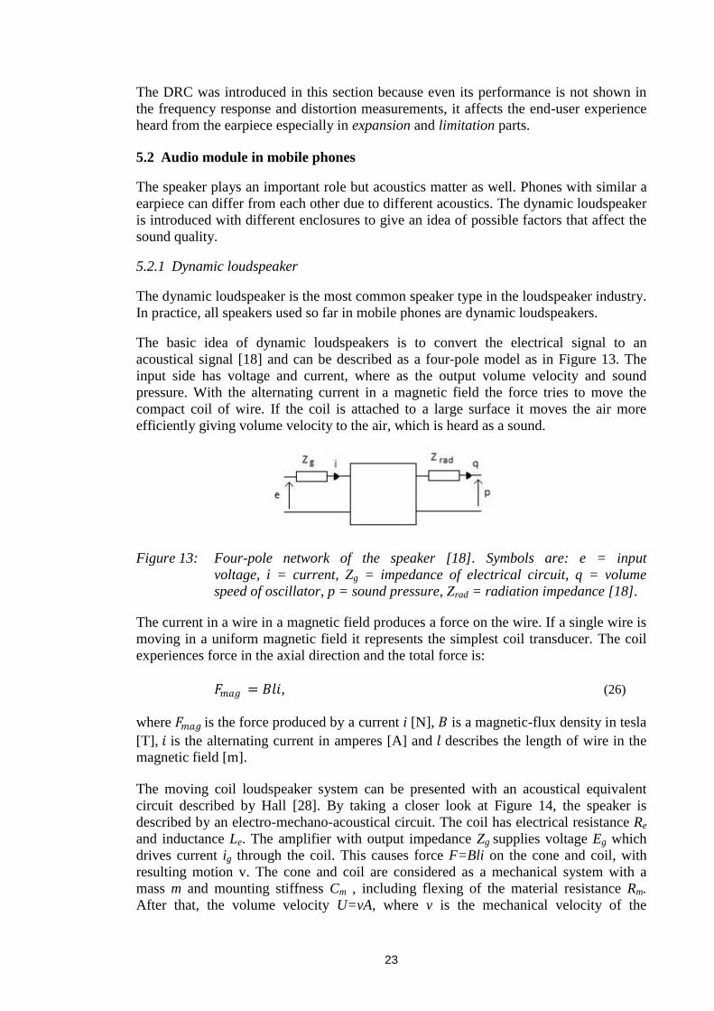
The basic idea of dynamic loudspeakers is to convert the electrical signal to an
acoustical signal [18] and can be described as a four-pole model as in Figure 13. The
input side has voltage and current, where as the output volume velocity and sound
pressure. With the alternating current in a magnetic field the force tries to move the
compact coil of wire. If the coil is attached to a large surface it moves the air more
efficiently giving volume velocity to the air, which is heard as a sound.
Figure 13: Four-pole network of the speaker [18]. Symbols are: e = input
voltage, i = current, Zg = impedance of electrical circuit, q = volume
speed of oscillator, p = sound pressure, Zrad = radiation impedance [18].
The current in a wire in a magnetic field produces a force on the wire. If a single wire is
moving in a uniform magnetic field it represents the simplest coil transducer. The coil
experiences force in the axial direction and the total force is:
𝐹𝑚𝑎𝑔 = 𝐵𝑙𝑖, (26)
where 𝐹𝑚𝑎𝑔 is the force produced by a current i [N], 𝐵 is a magnetic-flux density in tesla
[T], 𝑖 is the alternating current in amperes [A] and 𝑙 describes the length of wire in the
magnetic field [m].
The moving coil loudspeaker system can be presented with an acoustical equivalent
circuit described by Hall [28]. By taking a closer look at Figure 14, the speaker is
described by an electro-mechano-acoustical circuit. The coil has electrical resistance Re
and inductance Le. The amplifier with output impedance Zg supplies voltage Eg which
drives current ig through the coil. This causes force F=Bli on the cone and coil, with
resulting motion v. The cone and coil are considered as a mechanical system with a
mass m and mounting stiffness Cm , including flexing of the material resistance Rm.
After that, the volume velocity U=vA, where v is the mechanical velocity of the
24
membrane and A is cone area A. Volume velocity U works against the radiation
impedance Za,rad of the surrounding air to generate sound pressure p.
Figure 14: Electro-mechano-acoustical circuit of moving coil loudspeaker system.
The symbols are explained above the figure in the text [28].
The structure of a dynamic loudspeaker is quite simple. Usually the wire is wrapped as
a coil and situated between the magnetic poles. The purpose is to maximize the length
of the wire where the magnetic field is constant and perpendicular to the wire. As
mentioned earlier neither the coil itself does move much air, nor produce sound. The
efficiency is increased by attaching the coil to a movable, light and relatively large
surface diaphragm which carries lots of air along with it. Low frequencies generally
need a larger radiating area, whereas high frequencies are produced with a smaller area.
In larger speakers, or home stereo speakers, the diaphragm is usually a cone, which is
fairly stiff and light. The diaphragms in small speakers used in a mobile phones are also
quite stiff even though the material is thin.
By looking at Figure 15 the main parts [27] of the dynamic loudspeaker are shown in a
cross-section picture. However, exactly this kind of shape is not used in mobile phone
earpiece, but the principle is the same.
Figure 15: Cross-section sketch of a dynamic loudspeaker [27].
To minimize the non-linear response, the permanent magnet must be selected to
produce a constant field and the voice coil should always have the same amount of turns
in every displacement inside the gap between the poles [29]. The movement area of the
25
voice coil has to be limited in the constant field area, because if a coil exceeds that area
the magnetic force Bl drops causing non-linearity. Another problem occurs if the
speaker diaphragm movement distance is too long and exceeds the linear operation area,
which may cause mechanical damage to the speaker. In order to reduce impedance
variation, the chassis is made either to be able to conduct the heat away from the voice
coil or the chassis endures high temperatures and this way the voice coil stays in a
stable condition even in harder usage.
Voice coil suspensions keep the speaker membrane accurately centered in the magnet
gap, which is important enabling only the axial direction movement. One other function
of the suspension is that, when there is no signal, the membrane is returned back to the
equilibrium position.
The main reasons for using a dynamic speaker are the low operational voltage, small
size and low price. There are some drawbacks like low efficiency (usually 1%) and
frequency response, which is poor at low frequencies due small effective radiating area
and short membrane movement distance. The simulation of enclosure and speaker
element for design purpose is fairly straightforward due to the long history of dynamic
transducer studies.
5.2.2 Leak types, front and back cavity
A loudspeaker without an enclosure design does not provide very good acoustic
performance. Usually there are lots of compromises in mobile phone acoustic design
due purpose of use or mechanical design. The main purpose of mobile phone earpiece is
to reproduce speech, which has been narrowband until these days. In upcoming years,
there will be a need for wideband capability and that must be taken into account when
designing the acoustics for mobile phones. Therefore the front and back cavities with
different leak types are introduced in this section.
The front of the loudspeaker
There are two main possibilities to realize the front part of the speaker, called the front
resonator and open front.
Front resonator: The front cavity usually consists of the cavity itself and a cover with
sound holes. The purpose of the front cavity is to boost high frequencies thus reduce the
need for equalization. The other function is to provide protection against dust, water and
other external damage, which could be harmful for the speaker without the front cavity.
The disadvantage of the front cavity together with the sound holes is that it is a new
source of tolerance errors, but proper front cavity design can decrease the amount of
tolerance effects. Also, the cavity requires space, which is not available adequately in
mobile phone.
Open front: If there is no space for a front cavity, the speaker can be placed so near the
phone cover that the cavity is very small or does not exist. This way the acoustic
resonances are shifted to higher frequencies above the speech band, but the boosting
effect of the front resonator for the higher speech frequencies in the usable band is lost.
This leads to much heavier DSP equalization. In addition, the open-front design does
not include a lowpass feature, which can be used to filter out unwanted for example
radio frequency (RF) buzzing noise just above the speech signal band. Both of the
explained implements are shown in Figure 16.
26
Figure 16: Different mobile phone earpiece front realizations [31].
Back side of the loudspeaker
There are four main design and various hybrids available for designers to choose for the
back side of the loudspeaker.
Open back: The back of the loudspeaker is left open to the space of air inside the phone.
This method is the most common in all earpieces [31]. Even if the sound from the back
of the loudspeaker is routed through the PWB behind the speaker, the realization is
called open back. The advantages are ease of design and small space consumption.
Problems can occur on low frequencies if a large external leak is included in the
mechanics.
Closed back: In this case the loudspeaker has its back enclosed in a cavity that is sealed
or contains a small acoustically damped leak. The leak is only connected to ambient air
or air inside the phone, not to the ear. The good side of this is the isolation to the
microphone though the air path inside the phone. The downside is that the cavity should
be large, around a few cm3. In practice, the open back realization is preferred for its
small space occupation offering almost as good a result as the closed back.
Vented: The idea in vented back enclosure is to work as a bass booster. The earpiece has
a back cavity that is hermetically sealed apart from an opening with a defined cross-
sectional area and length (pipe) behind the loudspeaker. The gained resonator is tuned
near the lower limit of the frequency range of the earpiece. To make the vented structure
to work, the outer end of the vent has to be routed directly or indirectly to the user's ear.
If this is neglected and the vent is left inside the phone without acoustical connection to
ear, the performance will be worse than with other implementations. The reason for
using this design is the boosting effect for low frequencies with lower distortion thus it
is well suited for a small speaker in wideband designs. The problem with this design is
the same as with closed back design, which is the required large cavity.
Tube-loaded: The realization is about the same as vented construction, but this case the
cavity is much smaller and the vent is narrower and longer. The advantage of this
method is small bass boost, which is important in wideband implementations. Even a
relative small speaker with stiff suspension can reach low frequencies but the speaker
has to handle the required higher displacement.
27
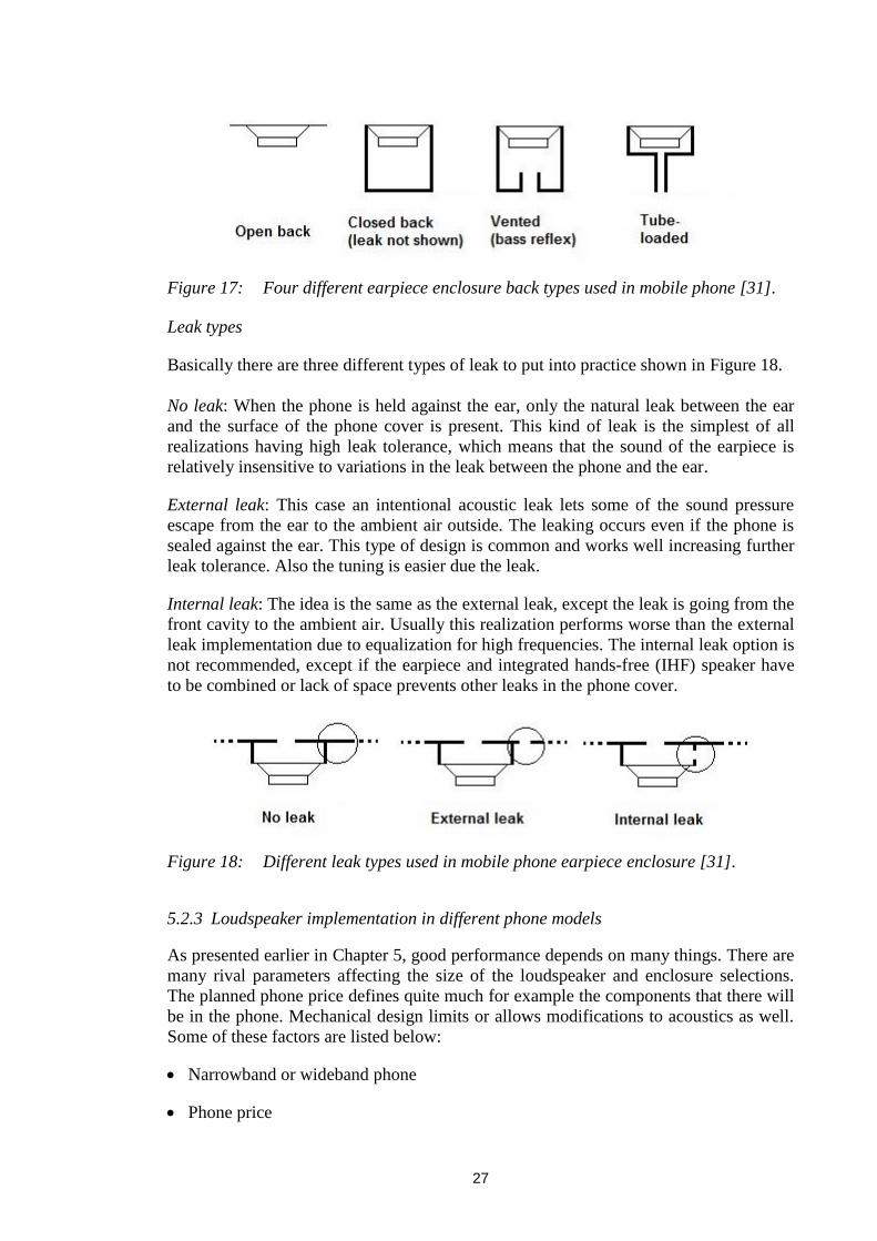
Figure 17: Four different earpiece enclosure back types used in mobile phone [31].
Leak types
Basically there are three different types of leak to put into practice shown in Figure 18.
No leak: When the phone is held against the ear, only the natural leak between the ear
and the surface of the phone cover is present. This kind of leak is the simplest of all
realizations having high leak tolerance, which means that the sound of the earpiece is
relatively insensitive to variations in the leak between the phone and the ear.
External leak: This case an intentional acoustic leak lets some of the sound pressure
escape from the ear to the ambient air outside. The leaking occurs even if the phone is
sealed against the ear. This type of design is common and works well increasing further
leak tolerance. Also the tuning is easier due the leak.
Internal leak: The idea is the same as the external leak, except the leak is going from the
front cavity to the ambient air. Usually this realization performs worse than the external
leak implementation due to equalization for high frequencies. The internal leak option is
not recommended, except if the earpiece and integrated hands-free (IHF) speaker have
to be combined or lack of space prevents other leaks in the phone cover.
Figure 18: Different leak types used in mobile phone earpiece enclosure [31].
5.2.3 Loudspeaker implementation in different phone models
As presented earlier in Chapter 5, good performance depends on many things. There are
many rival parameters affecting the size of the loudspeaker and enclosure selections.
The planned phone price defines quite much for example the components that there will
be in the phone. Mechanical design limits or allows modifications to acoustics as well.
Some of these factors are listed below:
Narrowband or wideband phone
Phone price
28
Dust and water protection
Mechanical design
Designer's set of parameters
If the phone is a wideband model the requirement for earpiece sound production
performance is different to narrowband. Using the small speaker gives more space for
other components in the phone and can be cheaper, but the low frequencies on
wideband cannot be reproduced as purely, or at all, as with a larger speaker. The
mechanical design containing cavities and leaks described earlier with DSP may help,
but a speaker has its limits and cannot break the physical laws. If the speaker is large,
lousy mechanical design or audio designers tuning parameters may be ruining the
advantages that could have been achieved by the speaker. On the other hand, using a
large speaker gives more margin to audio designers compared to small speakers.
29
6. OBJECTIVE MEASUREMENTS
It is important to show the objective results, when the subjective results are analyzed.
The purpose of objective measurements is to find out if there is any distinct differences
between the speakers 1) without the phones, 2) integrated to the phones without audio
processing and 3) integrated to the phones with audio processing. First, the theory of
objective measurements is presented and then the measurements with results of the used
phones and speakers are shown in this chapter.
6.1 Theory of audio measurements
Before the measurement results the theory behind the objective measurements are
presented in the next three sections. Impulse response, frequency response and
distortion methods are described to help to understand the measurement results later in
this chapter.
6.1.1 Transfer function
The transfer function describes an ideal system behavior with any kind of stimulus. An
ideal physical system has four properties [21]:
1) The system can be physically realized means that the system cannot produce an
output before input is applied.
2) Constant of its parameters when the system is time invariant thus the response of the
system is constant for all time values.
3) Stability limits the system's output to be a finite signal for a finite input signal.
4) A Linear system is additive and homogeneous. If the output signals are 𝑦1and 𝑦2 with
input signals 𝑥1 and 𝑥2. An additive system produces a summed output 𝑦1 + 𝑦2 from
summed input 𝑥1+ 𝑥2. A homogeneous output 𝑐𝑦1is produced from input 𝑐𝑥1, where c is
a random constant.
Figure 19: Linear, ideal system h(t) with one input x(t) and output y(t) signals [21].
The unit impulse function is defined as follows:
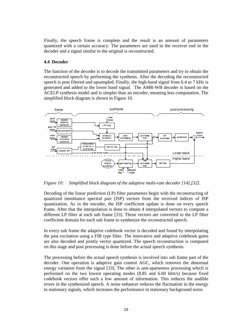
h(t) = y(t)
when
x(t) = (t)
Where h(t) is unit response function of the system, y(t) describes the output of the
system, x(t) input of the system and (t) is the ideal impulse, i.e. delta function, t is the
time from the moment when delta function enters the system. The duration of ideal
impulse is defined to approach to zero, so, in other words, the duration is infinitely
short. Also, the amplitude and energy is defined to be infinity and the integral equals 1
[22]. If the ideal impulse would be used for measuring the speakers of phones in this
30
thesis, the results with good signal-to-noise ratio would contain a high amount of
distortion, or even worse, break the speakers. It is obvious that these kind of parameters
are not for the practical part of this thesis but only for theory.
Instead of using the theoretical and unpractical method mentioned earlier, sine sweep is
used to measure the frequency response of the speakers. The simplest form of sine
swept frequency measurement is linearly or logarithmically variable sine wave, which is
fed to the device under measurement, DUT. Output signal represents the magnitude
response of the device.
Because the sinusoidal stimulus contains energy concentrated instantaneously at one
frequency, noise and other artifacts disturbing the measurement can be filtered away by
using tracking filter, i.e. a narrowband bandpass filter. One advantage of sine sweep is
its ability to measure simultaneously frequency response and the non-linear distortion
[36]. According to Farina in [36], from a sine signal used in an exponentially varied
frequency, it is possible to deconvolve simultaneously the linear impulse response of the
system and separate impulse responses for each harmonic distortion order.
6.1.2 Frequency response
When the system's output spectrum in response to an input signal is of interest, the
frequency response is the right measure. It often helps designers to implement systems
by offering additional information about the system behavior. The characteristics of the
system can be illustrated by a linear transform of the unit impulse response. The
transform function of a system can be represented in the Laplace form of the impulse
response.
𝐻 𝑠 = (𝑡)𝑒−𝑠𝑡𝑑𝑡∞
0 (27)
where H(s) is the complex-valued transfer function of a system and 𝑠 = 𝜎 + 𝑗𝜔
describes the complex frequency variable. The Laplace function, like the impulse
response is defined to begin at t = 0.
The most powerful method to represent the response in the frequency domain is the
Fourier transform [21] of the impulse response.
𝐻 𝑓 = 𝑡 𝑒−𝑗2𝜋𝑓𝑡∞
0𝑑𝑡 (28)
where H(f) is the complex frequency response of the system and f is the real-valued
frequency. When 𝜎 = 0 the Fourier transform (28) becomes the transfer function (27)
and it is investigated on the 𝑗𝜔-axis. The transfer function is not very practical and,
therefore, the frequency function is used instead. Usually, the absolute value of the
frequency response called the magnitude response |𝐻 𝑓 | describes the frequency
response curves.
The transform domain representation can be inversed to the time domain by inverse
Laplace in the s-domain or Fourier in the f-domain transform.
𝑡 =1
𝑗2𝜋 𝐻 𝑠 𝑒𝑠𝑡𝑑𝑠
𝜎+∞
𝜎−∞ (29)
𝑡 = 𝐻(𝑓)∞
−∞𝑒𝑗2𝜋𝑓𝑡𝑑𝑓 (30)
31
where 𝜎 is the real part of the complex frequency variable s.
6.1.3 Distortion
If a speaker with a completely linear transfer function would produce an identical output
signal compared to input signal there could not be any distortion. It is not a surprise that
a small speaker in mobile phone, capable of producing high sound pressure level cannot
play undistorted sound. The nonlinear distortion produces unwanted signal components,
which does not exist in original signal and adds them to the output signal.
The harmonic distortion appears on a clean sine sound in harmonic components. If the
spectrum of the signal consists of fundamental frequency A(1) and the amplitude of 𝑖𝑡 harmonic component A(i), the total harmonic distortion (THD) is defined [1] as
𝑑 = 100% 𝐴(𝑖)2𝑁
𝑖=2
𝐴(𝑖)2𝑁𝑖=1
(31)
where d is harmonic distortion, 𝐴(𝑖) is amplitude of 𝑖𝑡 harmonic component and N is
the number of harmonic components.
The distortion measurements in this thesis are done with all non-harmonic components,
background noise and noise from measurement equipment. This kind of distortion is
called THD+N. Not all distortion is a bad thing, mentioned in [1] that low order
harmonics can make the speech sound more pleasant in a telephone line than
undistorted speech.
6.2 Earpiece measurements in free field
The phones under measurements and the listening test have different size of speakers.
The physical measurements of the speakers are shown in Appendix A: and Appendix
B:. Those two speakers were measured in free field to obtain information about the
speaker performance before integrating it to the mobile phone. Both of the earpieces
were measured by Lauri Veko in the anechoic room (AR1) at the Salo Nokia premises
in November 2007.
6.2.1 Earpiece measurement procedure and equipment
The earpieces that were under evaluation were measured in the International
Electrotechnical Commission (IEC) standard baffle (a plate with a hole for speaker).
The used measurement setup was the following: The measurement adapters for both
speakers were free air adapters and designed for those two speakers. Basically, the
adapter had a hole in the front part, where the component sound hole was and the back
part was open. The measuring distance between the speaker and 1/4" free field
microphone was 1 cm. The whole measurement setup is shown in Figure 20. The
measuring equipment is listed in Table 2.
Table 2: Test equipment used in measurements of the earpieces in a baffle.
Instrument Type Comment
Audio Audio Precision Control software
measurement System Two ApWin
system Cascade
32
Instrument Type Comment
Audio Audio Precision Amos XG controls
Precision 2700 series Audio Precision, ApWin
Condensator B&K Type 4939 1/4" mic + its preamp
microphone + B&K Type 2670
preamplifier
microphone B&K Nexus Mic amplifier
amplifier
Impedance box 1ohm Shunt resistor
Rotel amplifier Speaker
amplifier with fixed gain +6dB amplifier
Figure 20: Speaker measurement set-up. A PC controls the Audio analyzer, which
brings the measurement data back to the computer.
6.2.2 Results of earpiece measurements
The speakers under evaluation were measured in a frequency range from 200 Hz to 20
kHz. The results of the frequency response measurement can be seen in Figure 21 and
distortion in Figure 22. The input voltage for both measurement was set to 0.179 Vrms.
Frequency response of the earpieces
If the wideband codec frequency range 50 - 7000 Hz is examined from the Figure 21,
the high frequency area near 7 kHz is about the same for both speakers. On the other
hand, at low frequencies, the small speaker performance is clearly worse than for the
large one. In fact, the frequencies under 400 Hz are 10 dB more silent on the small
speaker, which is not possible to compensate in the mechanical design and, therefore, is
seen later in earpiece integrated to phone in Section 6.3 results.
As can be seen from Figure 21 the large speaker frequency response curve -3 dB point
is around 300 Hz, when the small speaker has it at about 500 Hz. Also, the frequencies
between the two resonance peaks (big speaker 400 Hz-5000 Hz, small 600 Hz-7000 Hz)
varies in the large speaker only 4 dB and the small one 7 dB.
33
Figure 21: Small and large speaker frequency response in frequency range 200 Hz -
20 kHz measured with free air adapter.
Distortion in earpieces in free field
Distortion on both speaker is plotted in the same Figure 22 and notable thing is that
background noise is also included in the results. However, the small speaker has more
distortion below 650 Hz ending up to 11%. The frequency band is from 200 Hz to 20
kHz.
50
60
70
80
90
100
100 1000 10000
Mag
nit
ud
e r
esp
on
se [
dB
SP
L]
Frequency [Hz]
Speaker Frequency Response at 1mW (0.179Vrms)
Small speaker Large speaker
34
Figure 22: Small and large earpiece total harmonic distortion and noise in frequency
range 200 Hz - 20 kHz measured with free air adapter.
6.3 Measurement for wired earpieces integrated to Nokia mobile phone
After the free field measurements in Section 6.2, the speakers' performances can be
compared more or less in a theoretical aspect. If a speaker is measured in a free field
adapter it does not sound the same way when placed in a proper enclosure. Measuring
the earpieces wired to the phone means that the earpieces are integrated to the real
phone without the audio signal processing. Using the HATS' ear for measurement, the
results are one step closer to the end-user experience.
6.3.1 Selection criteria's for phones in the test
The phones that are measured in the next sections are introduced shortly before the
measurement procedure. Both of the phones were selected for this thesis on three
criterias: 1) Phones have different sized speakers 2) Support for AMR-WB codec
available, 3) is available on the market thus is not just a prototype. The other phone is a
Nokia 6220 classic introduced in Q208. It has the small speaker measured in Section
6.2. The other is the wideband phone, the Nokia 6720 classic, introduced in Q209.
Furthermore, it contains the large speaker.
6.3.2 Measurement equipment and procedure for wired earpieces
The idea of this measurement is to get data about the speakers integrated to the phone
without the influence of audio signal processing. The phones were positioned to HATS
according to the designers directions (Appendix F: and Appendix G:) and the phone
earpieces were wired directly to Audio Precision through a B&K power amplifier. After
the HATS ear the microphone signal was amplified in the B&K microphone multiplexer
and connected to a PC through Audio Precision. A block diagram of the measurement is
shown in Figure 23.
0,1
1
10
100 1000 10000
TH
D+
N [
%]
Frequency [Hz]
Speaker Total Harmonic Distortion and Noise at 1mW (0.179Vrms)
Small speaker Large speaker
35
Table 3: Used measurement equipment in HATS measurement by wiring the
earpieces directly to the power amplifier.
Instrument Type Comment
Audio Audio Precision Control software
measurement switcher Type ApWin
system SWR 2122
Audio Audio Precision Amos XG controls
Precision 2700 series Audio Precision, ApWin
Power B&K Type WR1105 Loudspeaker
amplifier amplifier
Microphone B&K Type 2822 Microphone
multiplexer amplifier
Before the actual measurement, the phone covers were opened and wires were soldered
to the earpiece springs. The proper soldering was confirmed with a multimeter by
measuring the speakers' resistances, which were about 30 Ω.
Figure 23: Measurement setup for phones measured on HATS by wiring the
earpieces.
The voltages used in the measurement were defined by Audio Precision and are
presented in Table 4.
Table 4: The input voltages for phone earpieces measured on HATS.
Type Input level [dBV] Input level [mVrms]
ERP -20 114
DRP -20 114
DRP -15 202.7
DRP -10 360.5
DRP -5 641.1
36
6.3.3 Results of the wired earpiece measurements on HATS
After the measurements Audio Precision plotted the results to Excel. The frequency
response and distortion results are shown below.
Frequency response
When phone measurements on HATS are plotted for different voltages, it can be seen
that the speaker performance is noticeably different, especially at lower frequencies.
There is a possibility to measure frequency response with ear-drum reference point
(DRP) or without ear reference point (ERP) the influence of HATS' ear auditory canal.
The reason for using DRP is that ERP measurement does not contain distortion
measurement in Audio Precision due to unlinear distortion at different frequencies.
Filtering the unlinear distortion would not be such a successful process. However, the
behavior of the speaker integrated to the phone is clearly shown in the DRP
measurements.
Figure 24: Frequency responses on range 100 - 8000 Hz measured on HATS using
different input voltage levels in N6720c and N6220c speakers.
The Ear Reference Point (ERP) results are shown for comparison for full audio path
measurements in Section 6.4. The Nokia 6220c is sealed on the HATS ear better than
the Nokia 6720c, which can be seen in Figure 25 at frequencies lower than 1 kHz. The
boosting effect from sealing helps the designer's tuning work to get the phone to fit into
the 3GPP frequency response mask. The descent of the frequency response of the Nokia
6220c from 600 Hz to 100 Hz is steeper than for the Nokia 6720c.
-20
-10
0
10
20
30
100 1000 10000
dB
Pa
Frequency [Hz]
Earpiece Power Compression on HATS DRP
Nokia 6220c -20dBV Nokia 6220c -15dBV Nokia 6220c -10dBV Nokia 6220c -5dBV
Nokia 6720c -20dBV Nokia 6720c -15dBV Nokia 6720c -10dBV Nokia 6720c -5dBV
37
Figure 25: Phones measured on HATS ERP position on frequency range 100 - 8000
Hz. HATS' ear effect is filtered away by Audio Precision measurement
system. THD+N
In the earpiece total harmonic distortion and noise (THD+N) measurement on different
voltages, the small speaker performs considerably poorly compared to the large speaker.
The distortion begins to rise faster than the large speaker under frequencies of 700 Hz.
The frequencies under 450 Hz for the small speaker THD+N results are inaccurate due
the incapability of reproducing such low frequencies. Basically, the membrane is so
small that sound production is impossible at those frequencies.
-20
-10
0
10
20
30
100 1000 10000
dB
Pa
Hz
Earpiece Frequency Response at -20 dBV at ERP
Nokia 6220c Nokia 6720c
38
Figure 26: Nokia 6720c and 6220c THD+N on different earpiece input voltages on
HATS. Measured frequency range is 100 - 8000 Hz.
6.4 Nokia mobile phone measurements over the air
The objective 3GGP [26] measurements of two Nokia phone models are shown in this
section. The idea is to compare over the air results to the speaker measurements done in
Section 6.2. It is also important to get information about the speaker integration and
audio path effects in the measurement results. These results describe the end user
hearing experience during a call.
6.4.1 Information about the phones in the test
All mobile phones that are on the market have been measured in a type approval test.
For this test, the designer defines the nominal volume level, which is a volume level
between 2/10-9/10. The selected nominal volume levels for both phones are shown in
Table 5. These volumes were used because the phones have been tuned to fit to the
masks on these specific levels.
Table 5: Nominal volumes of two Nokia phones.
Nokia 6220c
narrowband
Nokia 6220c
wideband
Nokia 6720c
narrowband
Nokia 6720c
wideband
Nominal volume 5 4 6 6
The AMR-WB speech codec was enabled in both phones for the tests.
0
10
20
30
40
50
100 1000 10000
Dis
tort
ion
%
Frequency [Hz]
Earpiece THD+N on HATS
Nokia 6220c -20dBV Nokia 6220c -15dBV Nokia 6220c -10dBV Nokia 6220c -5dBV
Nokia 6720c -20dBV Nokia 6720c -15dBV Nokia 6720c -10dBV Nokia 6720c -5dBV
39
6.4.2 Measurement equipment and procedure
Both of the phones were measured on HATS with 3GPP specification release 7 [26].
3GPP specifies test methods to allow the minimum performance requirements for the
acoustic characteristics of GSM and 3G terminals for both narrow and wideband. The
used measurement equipment in 3GPP measurements were proceeded with the list of
instruments in Table 6. This is the only measurement where Audio Precision was
replaced by Audio analyzer UPL-16.
Table 6: Equipment used in 3GPP measurements.
Instrument Type Comment
Radio Rohde & Schwarz GSM & WCDMA
communication CMU 200 network used
tester
Rohde & Schwarz Audio analyzer Sents result data to PC
UPL-16 Amos XG controls it
Head And Torso B&K Includes artificial ear
Simulator with microphone
microphone B&K Nexus HATS mic amplifier
amplifier +20dB
Once the phone was positioned to HATS the measurement was started. A PC controlled
the UPL, which fed the measurement signal to the radio communication tester and the
phone earpiece speaker signal was measured on the HATS' ear. Finally, the recorded
signal from the HATS ear is amplified 20 dB with B&K Nexus. The procedure is shown
in Figure 27.
Figure 27: Measurement setup for phone speaker frequency response and
distortion.
A picture of HATS used in this measurement and later in Section 7.2 for recording the
files for subjective test is shown in Figure 28.
40
Figure 28: Nokia 6720 classic positioned to 3GPP measurements HATS in
anechoic chamber.
Network settings for both phones were as in Table 7.
Table 7: CMU network settings in 3GPP HATS measurement.
GSM WCDMA
PCL 5 Uplink 1852.4 MHz
TCH 35 Downlink 1932.4 MHz
Codec mode 12.20 kbits Codec mode 12.65 kbps
Speech codec low Speech codec low
6.4.3 Measurement results
To ensure that the phone to be used in the recordings for subjective test is not a faulty
one, five phones of each model were measured. An average phone was selected based
on frequency response and distortion measurements. Differences in results between the
measured phones results were mostly inside ±1 dB.
Frequency response
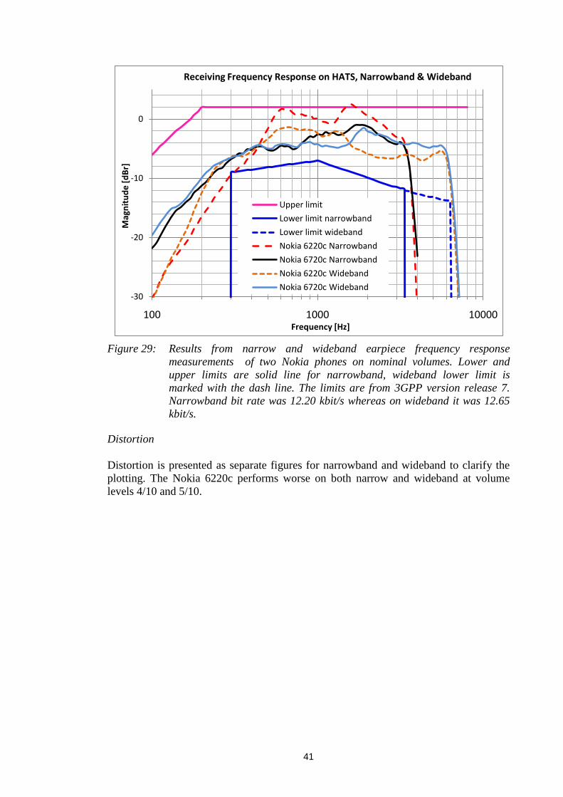
The frequency response follows the results in the previous Section 6.3.3. The Nokia
6720c has a flat response, while the Nokia 6220c fails to stay within the limits on
narrowband (red dash line in Figure 29).
41
Figure 29: Results from narrow and wideband earpiece frequency response
measurements of two Nokia phones on nominal volumes. Lower and
upper limits are solid line for narrowband, wideband lower limit is
marked with the dash line. The limits are from 3GPP version release 7.
Narrowband bit rate was 12.20 kbit/s whereas on wideband it was 12.65
kbit/s.
Distortion
Distortion is presented as separate figures for narrowband and wideband to clarify the
plotting. The Nokia 6220c performs worse on both narrow and wideband at volume
levels 4/10 and 5/10.
-30
-20
-10
0
100 1000 10000
Mag
nit
ud
e [
dB
r]
Frequency [Hz]
Receiving Frequency Response on HATS, Narrowband & Wideband
Upper limit
Lower limit narrowband
Lower limit wideband
Nokia 6220c Narrowband
Nokia 6720c Narrowband
Nokia 6220c Wideband
Nokia 6720c Wideband
42
Figure 30: Measured earpiece distortions on narrowband on nominal and maximum
volumes. Narrowband bit rate was 12.20 kbit/s and wideband bit rate was
12.65 kbit/s.
The difference between narrowband and wideband measurement result on the Nokia
6220c is emphasized by the volume level. The lower the volume, the more distortion
there is in lower signal levels.
Figure 31: Measured earpiece distortions on wideband using nominal and maximum
volumes. Narrowband bit rate was 12.20 kbit/s and wideband bit rate was
12.65 kbit/s.
0
10
20
30
40
50
60
-50 -40 -30 -20 -10 0
Ou
tpu
t SN
R [
dB
]
Input signal level [dB]
Narrowband Earpiece Distortion and noise on HATS, Nominal & Maximum Volume
Lower limit
Nokia 6220c Narrowband Volume 5
Nokia 6220c Narrowband Volume 10
Nokia 6720c Narrowband Volume 6
Nokia 6720c Narrowband Volume 10
0
10
20
30
40
50
60
-50 -40 -30 -20 -10 0
Ou
tpu
t SN
R [
dB
]
Input signal level [dB]
Wideband Earpiece Distortion and noise on HATS, Nominal & Maximum Volume
Lower limit
Nokia 6220c Wideband Volume 4
Nokia 6220c Wideband Volume 10
Nokia 6720c Wideband Volume 6
Nokia 6720c Wideband Volume 10
43
6.5 Discussions about the objective measurements
The objective measurements revealed expected differences between the small and large
speaker in capabilities of producing sound. The main reason for the differences in
results is the size of the earpiece membrane, which is discussed in the loudspeaker
theory Section 5.2.1 and seen in the free field measurement without being integrated to
the phone results in Section 6.2. After these it could be expected that there will be
differences in the results when the speakers are integrated to the phone and measured on
HATS.
Measurements on HATS illustrate the meaning of acoustics. If the measurements
without the phone audio processing are compared to 3GPP measurements where the
phone equalization and other audio enhancements are online, the results revealed that
audio processing can help to fix the problem by making the frequency response flatter.
The reason the frequency response is aimed to be flat is simply to avoid emphasizing or
diminishing certain frequencies, which could harm the understanding of hearing the
speech.
The incapability of reproducing low frequencies at a satisfying level for wideband
speech on a small earpiece can be seen from all measurements done in this chapter. The
distortion levels at different input voltage levels in Figure 26 revealed the unlinearity of
distortion on the small earpiece under frequencies of 450 Hz when the large earpiece
has fairly predictable levels until 100 Hz. In practice, the small earpiece may produce
audible distortion at low frequencies when the user sets the phone volume level to
maximum. Naturally, this limits the maximum output level that a designer can allow to
come out from the small earpiece without distortion. The other option is to damp the
low frequencies and allow the higher frequencies to sound louder. This option is
recommended only for narrowband speech and in the Nokia 6220c, the narrowband
speech is tuned to produce more higher frequencies (500 - 3000 Hz).
The differences of the two phone earpiece integration is shown on a theoretical level
and through objective measurements. The larger earpiece integration is 10 dB louder at
100 Hz and the fundamental frequency of male speech is around 100 Hz. After these
facts it can be said that the end-user should hear audible differences between the
realizations. The next chapter tries to find the answer to this and it is interesting to see
the subjective test results.
44
7. SUBJECTIVE TEST ON TWO EARPIECE INTEGRATIONS
The background of arranging the listening test is presented and the phases of processing
the subjective test files are described. In the end the listening test results are shown to
support the objective results.
7.1 Overview of subjective testing
Subjective testing is used in situations where there is no well-proven objective measure
of audio quality. The objective data can be used for speaker comparison, but the
objective measurements cannot be used in determining every audible characteristic of
the speaker. The problem is that human ears with brain analyzing do not process the
sound as microphones or measuring instruments do. When consumer buys a mobile
phone and listen to the speaker audio quality, the objective measurement data is not
available and this way the subjective experience becomes more important.
Subjective testing is a time consuming process, because a subject grades the
performance of many samples. Usually, the collected result data is quite sparse and
some variation occurs in identical samples due to the subject’s personal opinion.
However, proper test planning and constant testing conditions can decrease the variation
in the test results.
Performing a subjective test in an efficient way is a strict process. In [15] the following
procedure is suggested:
Definition of what is to be tested and null hypothesis
Selection of test paradigm
Creation of test material
Definition of sample population
Selection of listeners
Familiarization and/or training of subjects
Running the test
Analysis and reporting of results
7.1.1 Test type and listener selection
It is important to know that the selected test type affects the time consumption for
testing. There are several test methods to use for subjective testing [15]:
- Single stimulus, the mean opinion score (MOS) test belongs to absolute category
rating. Only one sample at a time is played and evaluated. The benefits are fast speed
and absolute rating.
- Paired comparison, A/B tests are for comparing relative quality of two samples A
and B. A few different possible comparison methods are:
o A or B, two possible options which is better.
45
o A or B scale, both samples are rated with the same scale.
o A or B scale with fixed reference is a test where one of the test samples is the
known reference and the other is a degraded from the reference.
o A or B scale with hidden reference is same as the previous but the reference is
not known, which enables either samples to be better.
- A, B or X test is made up of three samples. The idea is to choose, which one of two
samples, A or B is closer to the quality of X.
- A, B or C test is a triple stimulus comparison with a hidden reference. Two of three
samples are similar and one is the reference. The listener decides, which sample of
the other two samples is different to the reference and evaluates the sample.
- Rank order has several stimuli to compare. The relative order of the stimuli is rated.
Rapid ranking is a method of quality. The downside of it is that the perceptual
distance is unknown between the stimuli.
When the samples for the listening test were processed, it was time to decide the
listening test type. Because the differences between the small and large speaker are
rather small, the sensitive test type was needed. That's why the most convenient test
type for our purpose was A or B scale with a hidden reference. This method is quite
slow, but by choosing suitable amount of samples, the test duration was about 30 min
long.
The DaGuru listening test software has a few different choices for the mentioned (A/B
with hidden reference) test method and comparative mean opinion score 3 (CMOS3)
was selected. CMOS3 has a scale from -3 to 3, which was good enough for the purpose.
Choosing -3 means a lot worse and 3 a lot better than the first sample.
An important matter when setting up a listening test is the question of how many
subjects have to be recruited. Selecting the sample population type affects to the
decision about the size of the population as well as the reliability of the results. In [19]
listeners are divided into three groups:
- Naïve
o Subjects have not been selected for any discrimination or rating ability
o Subjects belong to the general public
o Discrimination and reliability skills are unknown
o In order to obtain low error variance, 24-32 listeners are required
- Experienced
o Subjects have experience in listening to a particular type of sound or product
o Experience does not promise reliability and repeatability
- Expert
o Tested subjects with normal hearing, good discrimination skill and reliability
o Subject may be over sensitive to aberrations in samples
o 10 subjects is enough for low error variance
46
7.2 Creation of test material
Before creating the listening test material the listening method had to be chosen. Several
different testing methods were discussed with the instructor of this thesis and Nokia
colleagues, resulting in three final options:
1) A real phone, listener hears a sample from a real phone in call, which is changed to
the other one after one sample is heard.
Real speaker implementation and call, speaker differences are possibly heard easier
in a noisy environment
Most accurate method as all interferences and problems of recording environment
are avoided
- The look of the phone affects the results
- Hard and laborious usage in the test, phones have to be switched many times
2) Rapid model, large and small speakers are integrated to identical rapid models, which
are changed after the sample is heard. Signal processing is done on the samples before
the test. Finally, samples are played from a laptop and fed to the speakers.
Real small and large speakers in use
The phones' look is identical and does not affect the evaluation
- Requires pre-work and signal processing before the files are ready for listening
- Hard and laborious usage in the test, phones have to be switched many times
3) Headphones, samples are recorded with HATS and processed before the test.
Samples are played from a laptop with headphones for the listeners.
Easy for listener
Listening test software can be used
No phone switching and effect on results by look
- Requires lots of work before the samples are ready for listening
- No real implementation
- Stages in signal processing diminishes large speaker advantages against small one
- Recording environment and sample processing adds interference to samples
Despite the heavy processing of samples the headphones were selected to be the
listening method for the samples. The ease of listening and answering with listening test
software was a big criteria to end up selecting the headphones. There was a plan to do a
listening test also in background noise and test intelligibility differences. Usage of
headphones was not feasible as the headphones damp the background noise.
Because the listening test was decided to proceed with headphones instead of using real
phones or rapid models, the sound files had to be processed to sound like a real phone
call in the listeners ear. Pre-processing the sound files was a laborious process, which is
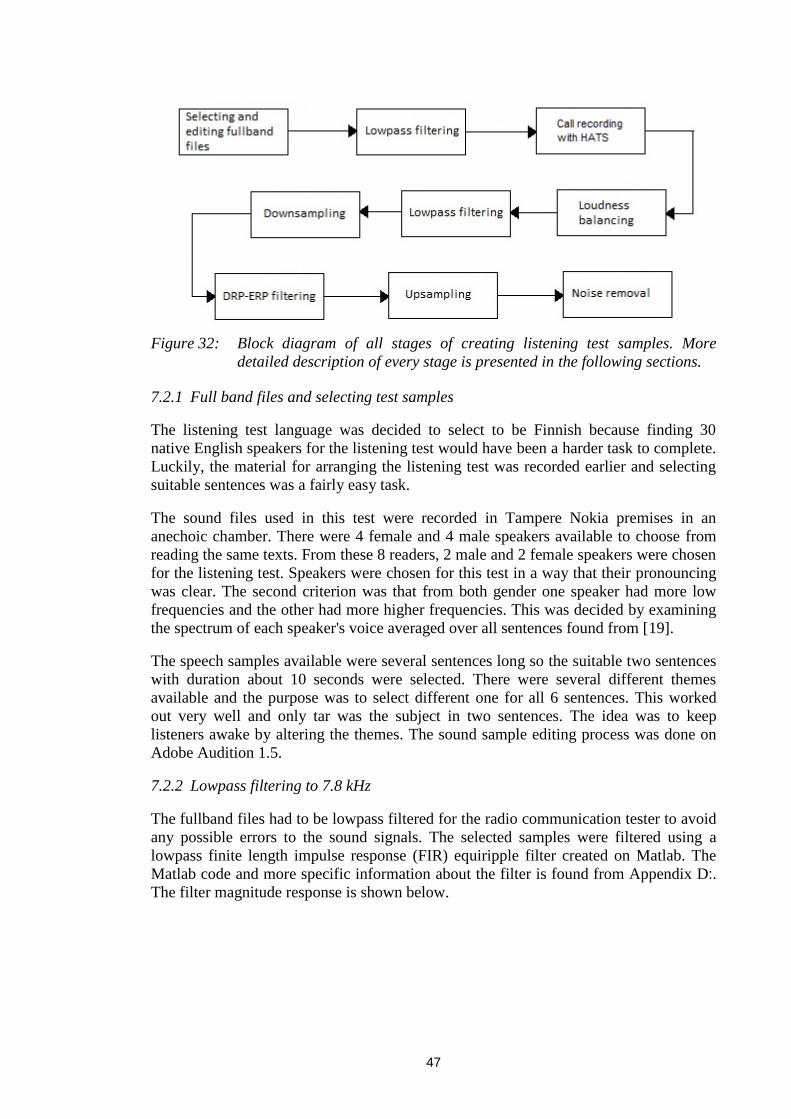
described in the nine-step block diagram in Figure 32.
47
Figure 32: Block diagram of all stages of creating listening test samples. More
detailed description of every stage is presented in the following sections.
7.2.1 Full band files and selecting test samples
The listening test language was decided to select to be Finnish because finding 30
native English speakers for the listening test would have been a harder task to complete.
Luckily, the material for arranging the listening test was recorded earlier and selecting
suitable sentences was a fairly easy task.
The sound files used in this test were recorded in Tampere Nokia premises in an
anechoic chamber. There were 4 female and 4 male speakers available to choose from
reading the same texts. From these 8 readers, 2 male and 2 female speakers were chosen
for the listening test. Speakers were chosen for this test in a way that their pronouncing
was clear. The second criterion was that from both gender one speaker had more low
frequencies and the other had more higher frequencies. This was decided by examining
the spectrum of each speaker's voice averaged over all sentences found from [19].
The speech samples available were several sentences long so the suitable two sentences
with duration about 10 seconds were selected. There were several different themes
available and the purpose was to select different one for all 6 sentences. This worked
out very well and only tar was the subject in two sentences. The idea was to keep
listeners awake by altering the themes. The sound sample editing process was done on
Adobe Audition 1.5.
7.2.2 Lowpass filtering to 7.8 kHz
The fullband files had to be lowpass filtered for the radio communication tester to avoid
any possible errors to the sound signals. The selected samples were filtered using a
lowpass finite length impulse response (FIR) equiripple filter created on Matlab. The
Matlab code and more specific information about the filter is found from Appendix D:.
The filter magnitude response is shown below.
48
Figure 33: The 7.8kHz lowpass filter magnitude response used to the full band
samples. Sampling rate was 48000Hz.
7.2.3 Call recording with HATS
The filtered files were played from a laptop and fed to a Rohde & Schwarz radio
communicator tester CMU. The laptop output signal level was adjusted according to the
CMU data sheet [37] to full-range input level in low sensitivity mode. The peak voltage
level is 1.4V and the laptop soundcard output RMS voltage level was supposed to be -
19.14 dBFS to prevent clipping of the speech signal. The required voltage level is
calculated from the following equation
𝐺𝑑𝐵 = 20log 𝑥
𝑉𝑟𝑒𝑓 (32)
−19,14𝑑𝐵 = 20𝑙𝑜𝑔 𝑥
1,4𝑉 (33)
𝑥 = 1,4𝑉 ∗ 10 −19,14
20 ≈ 155𝑚𝑉 (34)
where 𝐺𝑑𝐵 is the desired CMU input gain level in decibels, 𝑉𝑟𝑒𝑓 is the CMU maximum
input voltage peak level and 𝑥 is the CMU input voltage level for the desired decibel
value -19.14 dBFS and also the soundcard output voltage level. The result 155 mV was
measured from soundcard output when a -19 dBFS multitone was played by Adobe
Audition. The audio signal level in the phone's DSP was traced with a tracing device
(called Musti) to make sure the signal is not clipped before phone the earpiece. After
tracing showed that everything is in order, the phones were positioned to HATS and a
multitone signal was played from the laptop and volume levels were adjusted to be at a
suitable level for the actual recording process.
The CMU was used to make the call to the phone in a GSM 900 and WCDMA network.
Each phone was positioned to HATS according to the designer’s directions. The
received sound sample was recorded with HATS and amplified 20 dB on the B&K
Nexus amplifier. Finally, the samples were recorded on laptop using Adobe Audition. A
more detailed measurement setup is shown in Figure 34 and the equipment is described
below.
49
Table 8: Equipment used to record speech from phone earpiece placed on HATS.
Instrument Type Comment
Radio Rohde & Schwarz GSM & WCDMA
communication CMU 200 network used
tester
Head And Torso B&K Includes artificial ear
Simulator with microphone
microphone B&K Nexus HATS mic amplifier
amplifier
Sound card VX pocket 440 PCMCIA card with IBM
thinkpad T41
Phone signal Musti Speech signal level
tracker traced on phone DSP
Phone volumes were selected to be 6/10 and 10/10, because volume 6/10 is the level
that user would normally use in daily life and 10/10 is for the noisy environment. The
maximum level 10/10 was selected to find out if there is audible distortion in the
recordings with the small earpiece. Also, the speech signal level was higher and the
background noise was about the same, i.e. SNR was better than 6/10 level.
Figure 34: Measurement setup for live call recording with HATS. AS = Analog
Signal, RF = Radio Frequency.
7.2.4 Loudness balancing
When the samples were recorded with HATS, both the nominal and maximum volume
levels were used in the phones. It is said in [1] that usually the louder the sound is the
better it sounds to the listener. By aligning the sound level the loudness difference affect
is minimized and listeners can concentrate on evaluating correct affairs.
The balancing was done using the loudness batch tool version v1.4 and the following
parameters were given to the program: Input filename, align all samples to 27 Moore
average sones, align all samples to 27 Moore dynamic sones, align all samples to within
15% of the target sones. These parameters resulted in files having a peak amplitude of -
[36] Farina, A. Simultaneous Measurement of Impulse Response and Distortion
with a Swept-Sine Technique. AES 108th
convention. Paris. Preprint
No. 5093 (D-4). 2000. p 23.
[37] R&S CMU200 Universal Radio Communication Tester. Data sheet.
Version 08.01. 2007.
63
10. APPENDICES
APPENDIX A: Large speaker used in Nokia 6720c mobile phone
Figure 45: Large speaker dimensions used in Nokia mobile phone in listening test.
The dimensions are taken from [16].
Figure 46: Measures of the large speaker membrane used in Nokia mobile phone
in listening test.
64
APPENDIX B: Small speaker used in Nokia 6220c mobile phone
Figure 47: Small speaker dimensions used in Nokia mobile phone in listening test.
Dimensions are taken from [17].
Figure 48: Membrane measures of small speaker used in Nokia mobile phone in
listening test.
65
APPENDIX C: Listening test instructions (in Finnish)
Kuuntelukoeohje
Tässä kuuntelukokeessa kuunnellaan suomenkielisiä puhelinääninäytteitä. Näytteet
soitetaan pareittain, joista arvioidaan jälkimmäisenä kuultua näytettä verrattuna
ensimmäiseen asteikolla -3 (Paljon huonompi)…3 (Paljon parempi). Jos jälkimmäinen
on mielestäsi huonompi kuin ensimmäinen, valitse -3…-1. Jälkimmäisen ollessa
parempi kuin ensimmäinen, valitse 1...3. Jos et kuule eroa näytteiden välillä, valitse 0.
Arvioinnin perusteena on, kumpi näytteistä kuulostaa mielestäsi paremmalta.
Äänenvoimakkuus säädetään testin alussa kuuntelijalle sopivaksi, eikä sitä tarvitse
muuttaa testin aikana. Jos haluat kuulla näyteparin uudelleen, voit toistaa sen
enimmillään 2 kertaa, jottei testi mene liian pitkäksi.
Kun kuuntelukoe alkaa, ohjelma kysyy nimeäsi ja ikääsi. Voit kirjoittaa sen muodossa
NimiS 15V, jossa S on sukunimen ensimmäinen kirjain. Aluksi kuunnellaan 8
harjoitusnäyteparia, jonka jälkeen varsinainen testi alkaa. Tämän jälkeen kuunnellaan
25 paria nykyisin puhelimissa kuultavaa puhelinääntä, joiden jälkeen tulee 25 paria
tulevasta laajakaistaisesta puhelinäänestä.
Joissakin näytteissä voi olla häiriöitä (epäjatkuvuus, kohina), joita ei tarvitse huomioida
näytettä arvioidessa.
Laitathan kännykän äänettömälle testin ajaksi.
Jos kokeen aikana tulee kysyttävää, voit soittaa Sampalle 0440321069.
66
APPENDIX D: Matlab code for 7.8 khz filter
% 8kHz lowpass filter parameters (FIR equiripple)
% All frequency values are in Hz. Fs = 48000; % Sampling Frequency Fpass = 7700; % Passband Frequency Fstop = 8300; % Stopband Frequency Dpass = 0.057501127785; % Passband Ripple Dstop = 0.001; % Stopband Attenuation dens = 20; % Density Factor % Calculate the order from the parameters using FIRPMORD. [N, Fo, Ao, W] = firpmord([Fpass, Fstop]/(Fs/2), [1 0], [Dpass, Dstop]); % Calculate the coefficients using the FIRPM function. b = firpm(N, Fo, Ao, W, {dens}); % Sound file is read [x, fs, nbits] = wavread('input_file.wav'); % Sound file is filtered using filter specs above y = filter(b,1,x); % The frequency response of original sound file is calculated xF = 20*log10(abs(fft(x))); % The frequency response of original sound file is plotted figure(2); plot(xF,'g');
% Hold is done to plot both curves to same figure hold on; % The frequency response of filtered sound file is calculated yF = 20*log10(abs(fft(y))); % The frequency response of filtered sound file is plotted plot(yF,'r'); % Filtered sound file is written to hard drive wavwrite(y,Fs,nbits,'output_file');
67
APPENDIX E: Matlab code for 5.5 khz lowpass filter
% 5,5kHz lowpass filter parameters. % All frequency values are in Hz.
Fs = 48000; % Sampling Frequency Fpass = 5500; % Passband Frequency Fstop = 6400; % Stopband Frequency Dpass = 0.057501127785; % Passband Ripple Dstop = 0.001; % Stopband Attenuation dens = 20; % Density Factor % Calculate the order from the parameters using FIRPMORD. [N, Fo, Ao, W] = firpmord([Fpass, Fstop]/(Fs/2), [1 0], [Dpass, Dstop]); % Calculate the coefficients using the FIRPM function. b = firpm(N, Fo, Ao, W, {dens}); % Sound file is read [x, fs, nbits] = wavread('input_file.wav'); % Sound file is filtered using filter specs above y = filter(b,1,x); % The frequency response of original sound file is calculated xF = 20*log10(abs(fft(x))); % the frequency response of original sound file is plotted figure(2); plot(xF,'g'); hold on; % the frequency response of filtered sound file is calculated yF = 20*log10(abs(fft(y))); % the frequency response of filtered sound file is plotted plot(yF,'r'); % Filtered sound file is written to hard drive wavwrite(y,Fs,nbits,'output_file');
68
APPENDIX F: Type 4606 hats position table for Nokia 6720c
End stopper Support foot Front Rear
Endstop [mm] 13
Height[mm] 8 7
Offset [-5…5] 0 0
Centering fork Front Rear Socket position [1-5] Front 4
Offset [mm] 0 0 Spike [Position] +6,-6 +6,-6
Socket position [1-5] 1 5 Spike [Type] long long
Position Miscellaneous
DA [°] DB [°] DC [°] Pinna type Pressure force [N]
21 10 2,5 Soft 10
Nominal volume for Narrowband 6, Wideband 6
69
APPENDIX G: Type 4606 hats position table for Nokia 6220c
End stopper Support foot Front Rear
Endstop [mm] 16
Height[mm] 8 8
Offset [-5…5] 0 0
Centering fork Front Rear Socket position [1-5] Front 4
Offset [mm] 0 0 Spike [Position] +6,-6 +6,-6
Socket position [1-5] 2 3 Spike [Type] long long
Position Miscellaneous
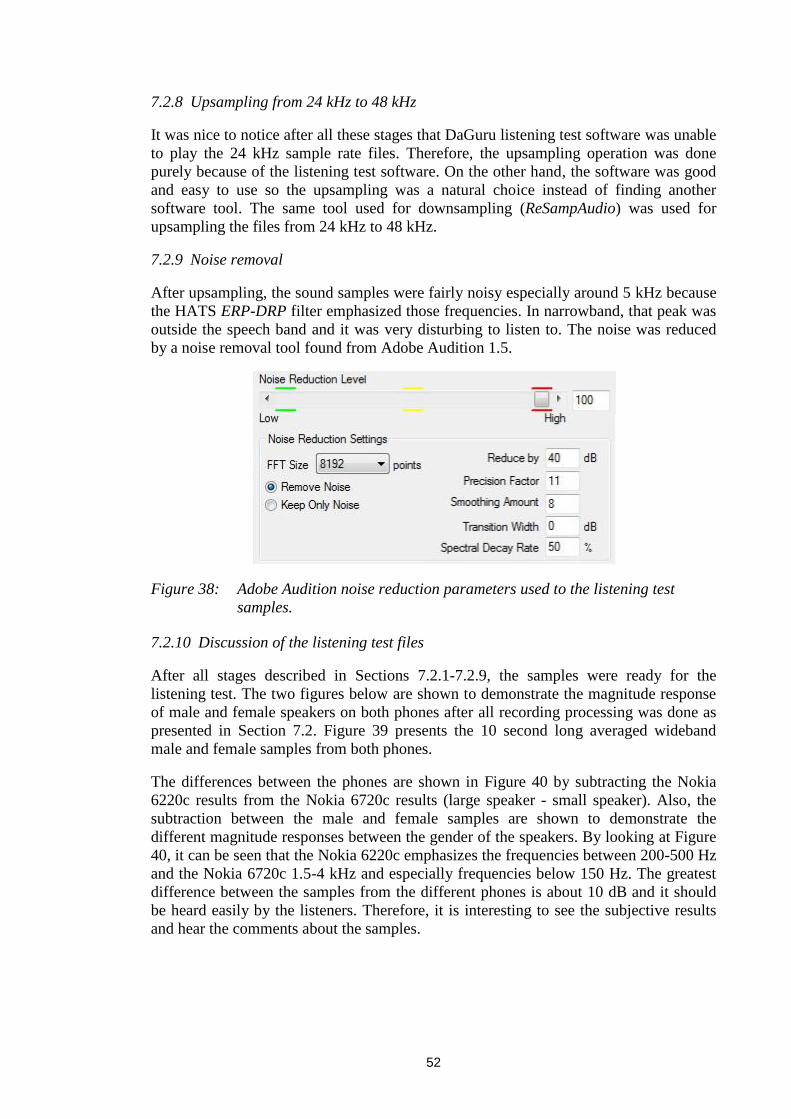
DA [°] DB [°] DC [°] Pinna type Pressure force [N]