JOURNAL OF SYMPLECTIC GEOMETRY Volume 2, Number 3, 309–355, 2004 SUBMANIFOLDS OF GENERALIZED COMPLEX MANIFOLDS Oren Ben-Bassat and Mitya Boyarchenko The main goal of our paper is the study of several classes of submanifolds of generalized complex manifolds. Along with the generalized complex submanifolds defined by Gualtieri and Hitchin in [Gua], [H3] (we call these “generalized La- grangian submanifolds” in our paper), we introduce and study three other classes of submanifolds and their relationships. For generalized complex manifolds that arise from complex (resp., symplectic) manifolds, all three classes specialize to complex (resp., symplectic) submanifolds. In general, how- ever, all three classes are distinct. We discuss some interest- ing features of our theory of submanifolds, and illustrate them with a few nontrivial examples. Along the way, we obtain a complete and explicit classification of all linear generalized complex structures. We then support our “symplectic/Lagrangian viewpoint” on the submanifolds introduced in [Gua], [H3] by defining the “generalized complex category”, modelled on the construc- tions of Guillemin-Sternberg [GS] and Weinstein [W2]. We argue that our approach may be useful for the quantization of generalized complex manifolds. Contents 1. Introduction 310 2. Generalized complex linear algebra 318 3. Generalized complex subspaces and quotients 323 4. Split subspaces and the graph condition 327 5. Generalized complex manifolds and submanifolds 331 6. The generalized complex “category” 336 7. Examples and counterexamples 338 309
Transcript
JOURNAL OFSYMPLECTIC GEOMETRYVolume 2, Number 3, 309–355, 2004
SUBMANIFOLDS OF GENERALIZED COMPLEXMANIFOLDS
Oren Ben-Bassat and Mitya Boyarchenko
The main goal of our paper is the study of several classes ofsubmanifolds of generalized complex manifolds. Along withthe generalized complex submanifolds defined by Gualtieriand Hitchin in [Gua], [H3] (we call these “generalized La-grangian submanifolds” in our paper), we introduce and studythree other classes of submanifolds and their relationships.For generalized complex manifolds that arise from complex(resp., symplectic) manifolds, all three classes specialize tocomplex (resp., symplectic) submanifolds. In general, how-ever, all three classes are distinct. We discuss some interest-ing features of our theory of submanifolds, and illustrate themwith a few nontrivial examples. Along the way, we obtain acomplete and explicit classification of all linear generalizedcomplex structures.
We then support our “symplectic/Lagrangian viewpoint”on the submanifolds introduced in [Gua], [H3] by defining the“generalized complex category”, modelled on the construc-tions of Guillemin-Sternberg [GS] and Weinstein [W2]. Weargue that our approach may be useful for the quantizationof generalized complex manifolds.
Contents
1. Introduction 310
2. Generalized complex linear algebra 318
3. Generalized complex subspaces and quotients 323
4. Split subspaces and the graph condition 327
5. Generalized complex manifolds and submanifolds 331
6. The generalized complex “category” 336
7. Examples and counterexamples 338
309
310 O. BEN-BASSAT AND M. BOYARCHENKO
8. Proofs 345
References 354
1. Introduction
1.1. Motivation. The goal of our paper is the study of certain specialclasses of submanifolds of generalized complex manifolds. The notion ofa generalized complex manifold was introduced by Nigel Hitchin in [H2].It contains as special cases both complex and symplectic manifolds. LaterMarco Gualtieri and Hitchin ([Gua], [H3]) have defined a class of subman-ifolds of generalized complex manifolds which they have called “generalizedcomplex submanifolds” and which in this paper we call “generalized La-grangian submanifolds”, for the reasons explained below. Hitchin’s andGualtieri’s notion specializes to complex submanifolds of complex manifoldsand to Lagrangian submanifolds of symplectic manifolds. In particular, if Mis a generalized complex manifold, then, in general, neither M itself nor thepoints of M are generalized complex submanifolds of M in their terminology.
Our first task, then, was to find a different definition which gives com-plex submanifolds in the complex case and symplectic submanifolds in thesymplectic case. It is also important to understand the relationship betweenour notion of a generalized complex submanifold and Hitchin and Gualtieri’snotion; and, on the other hand, to try to see if Hitchin and Gualtieri’s notioncan be used in the theory of generalized complex manifolds in a similar waythat Lagrangian submanifolds are used in symplectic geometry. For exam-ple, if φ : N → M is a diffeomorphism between two symplectic manifolds,it is well-known (see, e.g., [CdS]) that φ is a symplectomorphism if andonly if the graph of φ is a Lagrangian submanifold of N × M with respectto the “twisted product symplectic structure” on N × M . It is natural toask if the obvious generalization of this result holds for generalized complexmanifolds.
More generally, suppose (M, ωM ) is a symplectic manifold and N is asubmanifold of M which carries a symplectic form ωN . Again, it is easy tosee that ωN = ωM
∣
∣
Nif and only if the graph of the inclusion map N → M
is an isotropic submanifold of N × M with respect to the twisted productsymplectic structure. On the other hand, if M is a real manifold, N is asubmanifold of M , and both M and N are equipped with complex structures,then N is a complex submanifold of M if and only if the graph of theinclusion map N → M is a complex submanifold of N ×M with respect tothe product complex structure.
A starting point for our discussion is the observation that the conditionsappearing in Gualtieri and Hitchin’s definition of a generalized complex sub-manifold can be relaxed naturally, so that the resulting object specializes
SUBMANIFOLDS OF GENERALIZED COMPLEX MANIFOLDS 311
to complex submanifolds in the complex case and to isotropic submanifoldsin the symplectic case. We call these objects “generalized isotropic sub-manifolds.” One of the main goals of our work was trying to generalize theremarks of the previous paragraph to find a relationship between generalizedisotropic submanifolds and our notion of generalized complex submanifolds.
Another goal was to define and study the “generalized complex category”,in the spirit of [W1], [W2]. The definition is based on the notion of ageneralized Lagrangian submanifold. We believe that this “category” canbe used to study quantization of generalized complex manifolds. (The word“category” appears in quotes, because, as explained in [W1] or [W2], acertain transversality condition has to be satisfied for a pair of morphismsto be composable.)
The class of submanifolds which we call generalized complex submanifoldsis distinguished in that (in contrast to the others) its members naturally in-herit a generalized complex manifold structure from the ambient manifold.After the first version of our paper has appeared we have learned of a newdefinition of a class of submanifolds of generalized complex manifolds whichincludes the submanifolds introduced by Gualtieri and Hitchin as a sub-class. These submanifolds are called generalized complex branes in a recentpaper of Kapustin [Kap] on Topological Strings. We do not investigatethe relationships of generalized complex branes to the other submanifoldsintroduced in our paper.
1.2. Main results. Most of our paper is devoted to the study of generalizedcomplex structures on real vector spaces. Only at the end do we apply ourresults to generalized complex manifolds. While we feel that our study ofsubspaces of generalized complex vector spaces is more or less complete, it isclear that our results for generalized complex manifolds have a preliminarynature. Still, we believe that the questions that we have raised are alreadyfundamental at the vector space level and thus have to be addressed. Fur-thermore, as we show, the linear situation is far from being trivial (unlikein the theory of complex or symplectic vector spaces), due to the possibilityof a B-field transformation.1 Some unexpected features of the theory aredescribed below.
The first part of our paper is devoted to the study of induced general-ized complex structures on subspaces of generalized complex vector spaces.The situation is quite similar to the one considered by Theodore Courant in[Cou]. In fact, many of our basic constructions are straightforward modifi-cations of the ones introduced by Courant. However, there is an importantdifference: whereas a Dirac structure on a real vector space induces a Dirac
1These transformations, along with the β-field transformations, play a special role inthe theory. They were first introduced in [H2]. We recall their definition in §2.4.
312 O. BEN-BASSAT AND M. BOYARCHENKO
structure on every subspace and quotient space, this is not so for general-ized complex structures. Namely, recall that if V is a finite-dimensional realvector space, then a generalized complex structure on V can be defined by asubspace E ⊂ VC ⊕V ∗
Cwhich is isotropic with respect to the quadratic form
Q(v ⊕ f) = −f(v) and satisfies VC ⊕ V ∗C
= E ⊕ E, where the bar denotesthe complex conjugate. Now, given a real subspace W ⊆ V , we can define,as in [Cou], the subspace EW ⊂ WC ⊕ W ∗
Cconsisting of all pairs of the
form(
w, f∣
∣
WC
)
, where w ∈ WC and f ∈ VC are such that (w, f) ∈ E. It is
clear that EW is still isotropic with respect to Q. However, the conditionWC ⊕ W ∗
C= EW ⊕ EW may no longer hold.
Thus we define W to be a “generalized complex subspace” if the last con-dition does hold, so that we get an induced generalized complex structure.We then describe this induced structure in terms of spinors (Proposition3.5). The dual notion, that of a quotient generalized complex structure,is also studied. We introduce an operation which interchanges generalizedcomplex structures on a real vector space and on its dual; this operationcan then be used to reduce many statements about quotients to statementsabout subspaces (and vice versa). Hence, naturally, we devote more atten-tion to subspaces than to quotients. Since the original version of this paperwas made available we have realized that this duality operation correspondsto the idea of T-duality from the physics literature, see [KO, TW] and thereferences therein. This idea is used to establish a form of mirror symme-try for generalized complex manifolds in a recent preprint [B] by the firstauthor. We also prove the classification theorem for generalized complexvector spaces: every generalized complex structure is the B-field transformof a direct sum of a complex structure and a symplectic structure (Theo-rem 3.10). This result has applications to the study of constant generalizedcomplex structures on tori, both with regards to quantization and Moritaequivalence (cf. [TW]), and mirror symmetry (cf. [KO]).
At this point we should mention that there is some overlap between ourpaper and Gualtieri’s thesis [Gua]. Most notably, this applies to our clas-sification theorem mentioned above, which corresponds to Theorem 4.13 in[Gua]. However, the first version of our paper was placed on the e-Printarchive and submitted for publication before [Gua] became available to (usand) the general audience; in particular, we have obtained the classificationtheorem independently. Of course, many definitions given in our paper canbe found in [Gua]; they are given here for completeness, and our paper isself-contained and can be read independently of [Gua].
Let us emphasize that there are several subtle points in the theory of sub-spaces that we develop, which are not present in the theory of complex orsymplectic structures on vector spaces. For example, if W is a generalizedcomplex subspace of a generalized complex vector space V , then V/W need
SUBMANIFOLDS OF GENERALIZED COMPLEX MANIFOLDS 313
not be a generalized complex quotient of V (cf. Example 7.6). As anotherexample of “strange” behavior, we show the following. If V is any general-ized complex vector space, there is a unique maximal subspace S of V suchthat S is a GC subspace and the induced structure on S is B-symplectic(Theorem 3.11). [Hereafter, we use the expressions “B-symplectic struc-ture” and “B-complex structure” as shorthand for “B-field transform of asymplectic structure” and “B-field transform of a complex structure,” re-spectively.] Furthermore, there is a canonical complex structure J on thequotient V/S. However, V/S may not be a generalized complex quotient of
V , in the sense of Definition 3.8. (See Example 7.7.) On the other hand, ifV/S is a generalized complex quotient of V , then the induced structure onV/S is B-complex, and the associated complex structure coincides with J .
The interplay between B-field transforms and β-field transforms is alsodelicate. For instance, if a generalized complex structure is both a B-fieldtransform and a β-field transform of a (classical) complex structure, then itis, in fact, complex. The corresponding statement for symplectic structuresis false. On the other hand, it is possible to start with a classical symplecticstructure, make a B-field transform, then a β-field transform, and arrive ata classical complex structure. These features are discussed in some detail in§7.4.
To describe the results of the second part of the paper, we need to in-troduce more notation. Let V be as above, and recall that another way todescribe a generalized complex structure on V is by giving an automorphismJV of V ⊕V ∗ which satisfies J 2
V = −1 and preserves the quadratic form Q onV ⊕ V ∗. [An equivalence with the previous definition is obtained by assign-ing to such a JV its +i-eigenspace E in VC ⊕ V ∗
C.] For many considerations
it is convenient to write JV in matrix form:
JV =
(
J1 J2
J3 J4
)
,
where J1 : V → V , J2 : V ∗ → V , J3 : V → V ∗ and J4 : V ∗ → V ∗ are linearmaps.
Let W be a real subspace of V . We call W a generalized isotropic
(resp. generalized coisotropic, resp. generalized Lagrangian) subspace ofV if JV (W ) ⊆ W ⊕ Ann(W ) (resp. JV (Ann(W )) ⊆ W ⊕ Ann(W ), resp.W ⊕ Ann(W ) is stable under JV ). We say that W is split if there existsa subspace N ⊆ V such that V = W ⊕ N and W ⊕ Ann(N) ⊆ V ⊕ V ∗
is stable under J . [In fact, this is equivalent to the condition that thereis a decomposition V = W ⊕ N as a direct sum of generalized complexstructures, which explains the terminology.]
314 O. BEN-BASSAT AND M. BOYARCHENKO
On the other hand, we define the “opposite generalized complex struc-ture” on V to be the one corresponding to the automorphism
JV =
(
J1 −J2
−J3 J4
)
.
If W is equipped with some generalized complex structure JW , we say thatthis subspace satisfies the graph condition (with respect to JW ) if the graphof the inclusion map W → V is a generalized isotropic subspace of W ⊕V with respect to the “twisted product structure” on W ⊕ V , which bydefinition is the direct sum of JW and JV .
The following three results (see §4.4) explain the relations between thethree types of subspaces of a generalized complex vector space V that wehave introduced.
Theorem 1. Every split subspace is a generalized complex subspace. Fur-
thermore, it satisfies the graph condition with respect to the induced gener-
alized complex structure.
Theorem 2. A generalized complex subspace W ⊆ V satisfies the graph
condition with respect to the induced structure if and only if W is invariant
under J1.
It is worth emphasizing that if W is a generalized complex subspace andit satisfies the graph condition with respect to some generalized complexstructure, this structure does not necessarily have to be the induced one.More precisely:
Theorem 3. Suppose that W ⊆ V is an arbitrary subspace and JW is a
generalized complex structure on W such that the graph condition is satisfied.
If W is a generalized complex subspace, then the graph condition is also
satisfied with respect to the induced generalized complex structure, and JW
is a β-field transform of the induced structure on W .
In Remark 7.4, we show that a subspace satisfying the graph conditionwith respect to some generalized complex structure does not have to be ageneralized complex subspace in our sense. This may be seen as evidenceof the fact that our definition of the graph condition is too weak. Onepossible explanation for this is that, unlike the classical symplectic situation,a generalized isotropic subspace which has half the dimension of the ambientspace is not necessarily generalized Lagrangian. Thus, for example, if µ :V → W is an isomorphism of real vector spaces, and V , W are equippedwith generalized complex structures such that the graph of µ is generalizedisotropic with respect to the twisted product structure, then it does notnecessarily follow that µ induces an isomorphism between the two structures.On the other hand, we have the following
SUBMANIFOLDS OF GENERALIZED COMPLEX MANIFOLDS 315
Theorem 4. Let V , W be generalized complex vector spaces, and let µ :V → W be an isomorphism of the underlying real vector spaces. If the graph
of µ is generalized Lagrangian with respect to the twisted product structure on
V ⊕W , then µ induces an isomorphism between the two generalized complex
structures.
The global version of this result is given in Theorem 6.1.
In the second part of the paper we generalize all the notions introducedpreviously to generalized complex manifolds. In addition, we study theanalogue of the notion of an “admissible function” introduced by Courant[Cou]. This leads to the definition of the Courant sheaf: if M is a generalizedcomplex manifold, with JM the corresponding automorphism of TM⊕T ∗Mand E the −i eigenbundle of JM on TCM⊕T ∗
CM , the sections of the Courant
sheaf are pairs (f, X), where f is a complex-valued C∞ function and X is asection of TCM such that df +X ∈ E. We prove that the Courant sheaf is asheaf of local rings and also a sheaf of Poisson algebras. Moreover, for a splitsubmanifold N of a generalized complex manifold M , we define a naturaloperation of “pullback” of sections of the Courant sheaf on M to those on N(Theorem 5.13). The generalized complex structure on M can be recoveredfrom the Courant sheaf together with its embedding into C∞
M ⊕ TCM incase M is complex or symplectic, but it seems that, in general, additionalinformation is required.
The last part of the paper is devoted to the generalized complex “cat-egory”. Recall that Weinstein [W2] has introduced the symplectic “cate-gory”, based on some ideas of Guillemin and Sternberg [GS]. The objectsof this “category” are symplectic manifolds. If M and N are two symplecticmanifolds, the set of morphisms from M to N is defined to be the set ofsubmanifolds of M × N that are Lagrangian with respect to the “twistedproduct symplectic structure” on M × N . Two morphisms, M → N andN → K, can be composed provided a certain transversality condition issatisfied (see [W2] for details). In §6.2 we generalize Weinstein’s construc-tion by replacing symplectic manifolds with generalized complex manifolds,and Lagrangian submanifolds with generalized Lagrangian submanifolds. Inthe linear case (§6.3), where the transversality condition disappears, we getan honest category, thereby generalizing a construction of Guillemin andSternberg [GS]. We would like to point out that one of the applicationsof Guillemin-Sternberg-Weinstein construction is to deformation quantiza-tion and geometric quantization of symplectic manifolds (see [GS], wherethe quantization problem is solved completely in the linear case, and [W1],[W2] for a discussion of the global case). We hope that, similarly, the con-structions of Section 6 can be used for quantization of generalized complexstructures. We plan to study this in detail in subsequent publications.
316 O. BEN-BASSAT AND M. BOYARCHENKO
1.3. Structure of the paper. Our paper is organized as follows. In Sec-tion 2 we recall the basic definitions of the theory of generalized complexvector spaces. We follow [Gua] and [H3] for the most part. We also list thebasic definitions and results from the theory of spinors, referring to the book[C] for proofs. We then define an operation which interchanges generalizedcomplex structures on a real vector space with those on its dual, and weconclude the section with a discussion of B-field and β-field transforms. InSection 3 we introduce and study the notions of “generalized complex sub-spaces” (by modifying the construction of [Cou]) and “generalized complexquotients.” We also prove the classification theorem for generalized com-plex structures, as well as certain weaker but more “canonical” analoguesof the theorem; a consequence of our theory is that every generalized com-plex vector space has even dimension over R. In Section 4 we introduce thenotions of “split subspaces” and “subspaces satisfying the graph condition”and describe in detail the relationship of these notions with the more generalnotion of a generalized complex subspace.
In Section 5 we recall the definitions of generalized almost complex mani-folds and generalized complex manifolds. For the latter, we study the natu-ral generalization of the notion of “admissible function” defined by Courant,and we introduce the “Courant sheaf.” We then define the global analoguesof generalized complex subspaces and split subspaces: “generalized complexsubmanifolds” and “split submanifolds” of generalized complex manifolds.We end the section by defining the “pullback” of sections of the Courantsheaf on a generalized complex manifold to a split submanifold. In Section6, we study the “graph condition” for submanifolds of generalized complexmanifolds. This idea allows us to define the “generalized complex category”a la Weinstein [W2]. We finish by studying the simpler category of general-ized complex vector spaces, modelled on the construction of Guillemin andSternberg [GS].
In Section 7 we illustrate our main constructions and results with twotypes of examples: B-field transforms of complex and symplectic structures.(A few scattered examples also appear throughout the text.) More specif-ically, we characterize the GC subspaces (resp. subspaces satisfying thegraph condition, resp. split subspaces) of B-complex and B-symplectic vec-tor spaces, we characterize generalized isotropic (resp. coisotropic, resp.Lagrangian) subspaces of complex and symplectic vector spaces, and westate Gualtieri’s characterization of generalized Lagrangian submanifolds ofB-complex and B-symplectic manifolds. We then explain some interestingfeatures of B-field transforms of symplectic manifolds. Finally, we discussin detail some nontrivial counterexamples that we mentioned in §1.2.
We have only included the proofs of the most trivial results in the mainbody of the paper. All other proofs appear in a separate section (Section
SUBMANIFOLDS OF GENERALIZED COMPLEX MANIFOLDS 317
8) at the end of the article. This clarifies the exposition, and allows usto present our results in not necessarily the same order in which they areproved.
For the reader’s convenience, a more detailed summary appears at thebeginning of each section.
1.4. Acknowledgements. We are grateful to Marco Gualtieri for sharingsome of his notes with us, prior to the publication of his thesis. The contentof those notes was used in this paper via several of the definitions andconstructions of Sections 2, 5 and 7 as is noted in the appropriate places.We would also like to thank Tony Pantev for the suggestion to work ongeneralized complex manifolds, as well as for many useful comments on ourpaper and suggestions for improvement. Last but not least, we are indebtedto our referees for suggesting several essential improvements to the style ofour presentation and pointing out the missing references.
1.5. Notation and conventions. All vector spaces considered in this pa-per will be finite-dimensional. We will be dealing with both real and complexvector spaces. If V is a real vector space, we denote by VC its complexifica-tion. If W ⊆ V is a real subspace, we will identify WC with a subspace ofVC in the usual way. The complex conjugation on C extends to an R-linearautomorphism of VC which we denote by x 7→ x. Recall that a complexsubspace U of VC is of the form WC for some real subspace W ⊆ V if andonly if U = U .
The dual of a real or complex vector space V will be denoted by V ∗. Wewill always implicitly identify V with (V ∗)∗. If W ⊆ V is a real (resp.,
complex) subspace, we write Ann(W ) =
f ∈ V ∗
∣
∣
∣f∣
∣
W≡ 0
. Similarly, if
U ⊆ V ∗ is a real or complex subspace, we write Ann(U) =
v ∈ V∣
∣f(v) =
0 ∀ f ∈ U
.
If V is real, we identify (VC)∗ with (V ∗)C in the natural way. The naturalprojections V ⊕ V ∗ → V and V ⊕ V ∗ → V ∗, or their complexifications,will be denoted by ρ and ρ∗, respectively. We have the standard indefinitenondegenerate symmetric bilinear pairing 〈·, ·〉 on V ⊕ V ∗, given by2
〈v + f, w + g〉 = −1
2
(
f(w) + g(v))
for all v, w ∈ V, f, g ∈ V ∗.
We use the same notation for the complexification of 〈·, ·〉. Usually, if v ∈ Vand f ∈ V ∗, we will write either 〈f
∣
∣ v〉 or 〈v∣
∣ f〉 for f(v). The pairing 〈·, ·〉corresponds to the quadratic form Q(v + f) = −f(v).
The exterior algebra of a vector space V will be denoted by∧• V . If
x ∈ V and ξ ∈∧• V ∗, we write ιxξ for the contraction of x with ξ. An
element B ∈∧2 V ∗ will be identified with the linear map V → V ∗ that it
2Our convention here follows that of [H3].
318 O. BEN-BASSAT AND M. BOYARCHENKO
induces; similarly, an element β ∈∧2 V will be identified with the induced
linear map V ∗ → V . We will frequently consider endomorphisms of V ⊕V ∗.These will usually be written as 2 × 2 matrices
T =
(
T1 T2
T3 T4
)
,
with the understanding that T1 : V → V , T2 : V ∗ → V , T3 : V → V ∗ andT4 : V ∗ → V ∗ are linear maps. In this situation, elements of V ⊕ V ∗ will bewritten as column vectors: (v, f)t, where v ∈ V , f ∈ V ∗.
For us, a real (resp., complex) manifold will always mean a C∞ real (resp.,complex-analytic) finite-dimensional manifold. If M is a real manifold, byC∞
M we denote the sheaf of (germs of) complex-valued C∞ functions on M .We will denote by TM and T ∗M the tangent and cotangent bundles ofM , and by TCM and T ∗
CM their complexifications. The pairing 〈·, ·〉 de-
fined above at the level of vector spaces extends immediately to a pairing〈·, ·〉 : VC × V ∗
C→ C∞
M , where V is any vector bundle on M and VC is itscomplexification. The de Rham differential on
∧• T ∗CM will be denoted by
ω 7→ dω. For a section X of TCM , we will denote by ιX and LX the op-erators of contraction with X and the Lie derivative in the direction of X,which are C-linear operators on
∧• T ∗CM .
By a complex structure on a real vector space V we mean an R-linear au-tomorphism J of V satisfying J2 = −1. (Other authors call such a J an al-
most complex structure.) The following abbreviations will be frequently usedin our paper: GC=“generalized complex”, GAC=“generalized almost com-plex”, GCS=“GC structure”, GACS=“GAC structure”, GCM=“generalizedcomplex manifold”, GACM=“generalized almost complex manifold”.
2. Generalized complex linear algebra
2.1. Equivalent definitions. We begin by giving three ways of defining aGCS on a real vector space, and then showing their equivalence. We will seelater that in various contexts, one of these descriptions may be better thanthe others, but there is no description that is “the best” universally. Thuswe prefer to work with all of them interchangeably.
Proposition 2.1. Let V be a real vector space. There are natural bijections
between the following 3 types of structure on V .
(1) A subspace E ⊂ VC ⊕ V ∗C
such that E ∩ E = (0) and E is maximally
isotropic with respect to the standard pairing 〈·, ·〉 on VC ⊕ V ∗C.
(2) An R-linear automorphism J of V ⊕ V ∗ such that J 2 = −1 and J is
orthogonal with respect to 〈·, ·〉.(3) A pure spinor φ ∈
∧• V ∗C, defined up to multiplication by a nonzero
scalar, such that 〈φ, φ〉M 6= 0, where 〈·, ·〉M denotes the Mukai pairing
([C], [H2], [H3]).
SUBMANIFOLDS OF GENERALIZED COMPLEX MANIFOLDS 319
Remark 2.2. Our notation is different from the one of Gualtieri [Gua],who uses L ⊂ VC ⊕ V ∗
Cto denote a generalized complex structure, and E
the projection of the subspace L onto VC.
The terminology (3) is explained in §2.2 below, and the bijections aremade explicit in §8.1. A structure of one of these types will be called ageneralized complex structure on V , and a real vector space equipped witha GC structure will be called a generalized complex vector space.
Remark 2.3. In [H1], [H2] it is assumed from the very beginning thatgeneralized complex manifolds have even dimension (as real manifolds). Thereader may also assume that our GC vector spaces have even real dimension;this is used in an essential way in the arguments that involve spinors (cf.Theorem 2.5(2.5)). However, we can prove that, with the definitions of aGC structure on V in terms of E ⊂ VC ⊕ V ∗
Cor J ∈ AutR(V ⊕ V ∗), the
even-dimensionality of V is automatic (Corollary 3.12). We invite the readerto check that our proof of Corollary 3.12 does not depend on any statementsabout spinors. The result was also proved in [H3] by a different method (byshowing that a GC structure on a real manifold induces an almost complexstructure).
2.2. Recollection of spinors. Here we list the basic definitions and resultsfrom the theory of spinors, following [C] (and, in a few places, [H3]), thatwill be used in the sequel. Chevalley’s description of the theory is somewhatmore general than presented below; however, the reader should have nodifficulty modifying the notation and results of [C] to fit our situation.
Let V be a real vector space, and write V d = V ⊕V ∗. Recall the quadraticform Q(v+f) = −〈v
∣
∣ f〉 = −ιv(f) on V d. We let Cliff(V ) denote the Clifford
algebra of the complexification V dC
corresponding to the quadratic form Q.This means (see [C]) that Cliff(V ) is the quotient of the tensor algebra onV d
Cby the ideal generated by all expressions of the form e⊗e−Q(e), e ∈ V d
C.
Note that if E is any isotropic (w.r.t. Q) subspace of V dC
, then the subalgebraof Cliff(V ) generated by E is naturally isomorphic to the exterior algebra∧• E. In particular, Cliff(V ) contains S(V ) :=
∧• V ∗C
in a natural way. Wecall S(V ) the space of spinors. The subspaces of S(V ) spanned by formsof even and odd degree are denoted by S+(V ) and S−(V ), respectively. Wecall S+(V ) (resp., S−(V )) the space of even (resp., odd) half-spinors.
There exists a representation of Cliff(V ) on S(V ), with the action of thegenerating subspace V d
C⊂ Cliff(V ) being defined by
(v + f) · φ = ιvφ + f ∧ φ, v ∈ VC, f ∈ V ∗C , φ ∈ S(V ).
Let φ ∈ S(V ), φ 6= 0, and let E be the annihilator of φ in V dC
, with respect tothe action defined above. Observe that if e ∈ E, then 0 = e · e ·φ = Q(e) ·φ,whence Q(e) = 0. Thus Q
∣
∣
E≡ 0, so E is isotropic with respect to Q.
320 O. BEN-BASSAT AND M. BOYARCHENKO
Definition 2.4. We say that φ is a pure spinor if E is maximally isotropic,i.e., dimC E = dimR V . In this case, we also call φ a representative spinor
for E.
Recall from §1.5 that complex conjugation acts on V dC
and on S(V ). It isclear that φ ∈ S(V ) is a pure spinor if and only if φ is such; and if φ is arepresentative spinor for a maximally isotropic subspace E ⊂ V d
C, then φ is
a representative spinor for E, and vice versa.
The last ingredient that we need is the Mukai pairing 〈·, ·〉M : S(V ) ×S(V ) →
∧n V , where n = dimR V (see [C], §III.3.2; [H2], [H3]). However,we have decided to omit the definition of this pairing, since it is describedin detail in [C] and [H3]. The only fact that we need about this pairingis Theorem 2.5(2.5), which is proved in [H3]. We refer the reader to [H3]for a detailed discussion of the Mukai pairing that is most relevant to oursituation.
We can now state the main results from the theory of spinors that we willuse in the paper.
Theorem 2.5.
(a) Every pure spinor is either even or odd: if φ ∈ S(V ) is pure, then
φ ∈ S+(V ) or φ ∈ S−(V ).(b) Let E ⊂ V d
Cbe a maximally isotropic subspace; then the space
AE =
φ ∈ S(V )∣
∣e · φ = 0 ∀ e ∈ E
is one dimensional. Thus the nonzero elements of AE are precisely
the representative spinors for E. In other words, we have a bijective
correspondence between maximally isotropic subspaces of V dC
and pure
spinors modulo nonzero scalars.
(c) Let E, F ⊂ V dC
be maximally isotropic subspaces corresponding to pure
spinors φ, ψ ∈ S±(V ). Then E ∩ F = (0) if and only if 〈φ, ψ〉M 6= 0.(d) In particular, if E ⊂ V d
Cis a maximally isotropic subspace correspond-
ing to a pure spinor φ, then E ∩ E = (0) if and only if 〈φ, φ〉M 6= 0.(e) A spinor φ ∈ S(V ) is pure if and only if it can be written as
(2.1) φ = c · exp(u) ∧ f1 ∧ · · · ∧ fk,
where c ∈ C×, u ∈
∧2 V ∗, and f1, . . . , fk are linearly independent ele-
ments of V ∗C. If φ is representative for a maximally isotropic subspace
E ⊂ V dC, then f1, . . . , fk form a basis for E ∩ V ∗
C.
(f) Suppose that dimR V is even, and let φ ∈ S(V ) be a pure spinor written
in the form (2.1). Then, up to a nonzero scalar multiple, we have
〈φ, φ〉M = (u − u)p ∧ f1 ∧ · · · ∧ fk ∧ f1 ∧ · · · ∧ fk,
where p = n/2 − k.
SUBMANIFOLDS OF GENERALIZED COMPLEX MANIFOLDS 321
Proofs. (a) [C], III.1.5. (b) The proof is contained in [C], §III.1. (c) [C],III.2.4. (d) This is immediate from (c). (e) [C], III.1.9. (f) See [H3]. ¤
2.3. Duality. Given a real vector space V , let τ : V ⊕ V ∗ → V ∗ ⊕ V bethe transposition of the two summands. Recalling the natural identificationof V ∗∗ with V , we can also view τ as an isomorphism between V ⊕ V ∗
and V ∗ ⊕ V ∗∗. We will continue to denote by τ the induced isomorphismVC ⊕ V ∗
C→ V ∗
C⊕ V ∗∗
C∼= V ∗
C⊕ VC. This duality operation corresponds to
the idea from the physics literature of T-duality, see [KO, TW] and thereferences therein. An explicit formula for the spinor representing the dualGC structure on V ∗ in terms of the spinor representing the GC structure onV turns out to be a Fourier-Mukai type of transformation, as in explained in[B] in relationship to a version of mirror symmetry for generalized complexmanifolds.
Proposition 2.6. The isomorphism τ induces a bijection between GC struc-
tures on V and GC structures on V ∗. Explicitly, E ⊂ VC⊕V ∗C
is a GCS on Vif and only if τ(E) is a GCS on V ∗. If E corresponds to J ∈ AutR(V ⊕V ∗)as in Proposition 2.1, then τ(E) corresponds to τ J τ−1.
Proof. If is clear that τ preserves the form 〈·, ·〉, and if E ⊆ VC ⊕ V ∗C
is any
subspace, then τ(E) = τ(E). The proposition follows trivially from theseobservations. ¤
2.4. B- and β-field transforms. Let V be a real vector space and B ∈∧2 V ∗. We form the matrix (see §1.5)
B :=
(
1 0B 1
)
.
It is straightforward to verify that B is an orthogonal automorphism ofV ⊕ V ∗. Thus, if E is a GCS on V , then B ·E is another one. We call B ·Ethe B-field transform of E defined by B.
Remark 2.7. The notion of a “gauge transformation” for Dirac structureshas been introduced and studied by Severa and Weinstein in [SW], §3. Theobvious complex analogue of this notion gives rise to the B-field transformsthat we have just defined.
Similarly, if β ∈∧2 V , then the matrix
B′ :=
(
1 β0 1
)
also acts on GC structures on V ; if E is one, then B′ · E will be called theβ-field transform of E defined by β. If we look at GC structures in terms ofthe corresponding orthogonal automorphisms J of V ⊕V ∗, then the actionsof B and β are given by J 7→ B ·J ·B−1 and J 7→ B′ · J ·B′−1, respectively.We can also describe B-field transforms in terms of spinors:
322 O. BEN-BASSAT AND M. BOYARCHENKO
Proposition 2.8. Suppose that a GCS on a real vector space V is defined
by a pure spinor φ ∈∧• V ∗
C, and let B ∈
∧2 V ∗. Then the B-field transform
of this structure corresponds to the pure spinor exp(−B) ∧ φ.
We leave to the reader the task of describing β-field transforms in a similarway.
Remark 2.9. Suppose that E is a GCS on a real vector space V and E′ isthe B-field transform of E defined by B ∈
∧2 V ∗. Then, obviously, τ(E′) is
the β-field transform of τ(E), defined by the same B ∈∧2 V ∗ (but viewed
now as a bivector on V ∗). Thus, the operation τ interchanges B- and β-fieldtransforms.
Definition 2.10. Let V be a real vector space.
(1) Let J be a (usual) complex structure on V . Then
J =
(
J 00 −J∗
)
is a GC structure on V . If J is a GCS on V that can be written in thisform, we say that J is complex.
(2) A B-field (resp., β-field) transform of a complex GCS on V will bereferred to as a B-complex (resp., β-complex) structure on V .
(3) Let ω be a symplectic form on V (i.e., a nondegenerate form ω ∈∧2 V ∗).
Then
J =
(
0 −ω−1
ω 0
)
is a GC structure on V . If J is a GCS on V that can be written in thisform, we say that J is symplectic.
(4) A B-field (resp., β-field) transform of a symplectic GCS on V will bereferred to as a B-symplectic (resp., β-symplectic) structure on V .
Proposition 2.11. Let V be a real vector space and E ⊂ VC ⊕ V ∗C
a GCS
on V . Write
J =
(
J1 J2
J3 J4
)
for the corresponding orthogonal automorphism of V ⊕ V ∗. Then
(a) E is B-complex (resp., β-complex) ⇐⇒ ρ(E) ∩ ρ(E) = (0)(
resp.,
ρ∗(E) ∩ ρ∗(E) = (0))
⇐⇒ J2 = 0 (resp., J3 = 0) ⇐⇒ V ∗C
=
(V ∗C∩ E) + (V ∗
C∩ E)
(
resp., VC = (VC ∩ E) + (VC ∩ E))
;
(b) E is complex if and only if it is both B-complex and β-complex;
(c) E is B-symplectic (resp., β-symplectic) ⇐⇒ E∩V ∗C
= (0)(
resp., E∩
VC = (0))
⇐⇒ J2 is an isomorphism (resp., J3 is an isomorphism)⇐⇒ ρ(E) = VC (resp., ρ∗(E) = V ∗
C);
(d) E is symplectic if and only if J1 = 0.
SUBMANIFOLDS OF GENERALIZED COMPLEX MANIFOLDS 323
The analogue of part (b) fails in the symplectic case, as we will see in§7.4.
3. Generalized complex subspaces and quotients
3.1. Definition of GC subspaces. Let V be a real vector space with aGC structure E ⊂ VC ⊕ V ∗
C. Given a subspace W ⊆ V , we define (following
[Cou])
(3.1) EW =
(
ρ(e), ρ∗(e)∣
∣
WC
)
∣
∣
∣e ∈ E ∩(
WC ⊕ V ∗C
)
.
Clearly, EW is an isotropic subspace of WC ⊕ W ∗C. It is straightforward to
compute that dimC EW = dimR W (see Lemma 8.2); thus EW is, in fact,maximally isotropic.
Remark 3.1. The definition of EW and the fact that it is maximallyisotropic can be obtained by specializing the much more general discus-sion of the functorial properties of linear Dirac structures, cf. [BR]. Wehave included the proof in our paper for the sake of completeness.
Definition 3.2. We say that W is a generalized complex subspace of V ifEW ∩ EW = (0), so that EW is a generalized complex structure on W .In this case, we denote by JW the orthogonal automorphism of W ⊕ W ∗
corresponding to EW .
We note that a Dirac structure on a real vector space V induces a Diracstructure on every subspace of V (see [Cou]). In our situation, however, notevery subspace of a GC vector space is a GC subspace. The reason is theextra condition EW ∩ EW = (0), which has no counterpart in the theory ofDirac structures.
Examples 3.3.
(1) Consider a complex GCS on V , corresponding to a complex structure Jon V . Then a real subspace W ⊆ V is a GC subspace if and only if Wis stable under J . In this case, the induced GC structure on W is alsocomplex, corresponding to J
∣
∣
W.
(2) Consider a symplectic GCS on V , corresponding to a symplectic formω on V . Then a real subspace W ⊆ V is a GC subspace if and only ifω∣
∣
Wis nondegenerate on W . In this case, the induced GC structure on
W is also symplectic, corresponding to ω∣
∣
W.
This follows from Proposition 7.1, where we give a complete descriptionof GC subspaces of B-complex and B-symplectic vector spaces.
Remark 3.4. In general, it seems that if W is a GC subspace of a GC vectorspace V , then there is no simple relationship between JW and JV . Laterwe will see that such a relationship exists for special types of GC subspaces.
324 O. BEN-BASSAT AND M. BOYARCHENKO
It is important to understand the passage from a GCS on V to the inducedGCS on a GC subspace W ⊆ V in terms of spinors. To that end, we havethe following
Proposition 3.5. Let V be a real vector space with a GC structure E ⊂VC ⊕ V ∗
C. Let W ⊆ V be any subspace, and let j : W → V denote the
inclusion map. Then there exists a representative spinor for E of the form
φ = exp(u)∧f1∧· · ·∧fk, such that, for some 1 ≤ l ≤ k, j∗(f1), . . . , j∗(fl) are
a basis of Ann(
ρ(E)∩WC
)
⊆ W ∗C, and fl+1, . . . , fk are a basis of Ann
(
ρ(E)+
WC
)
. Moreover, φW := exp(j∗u) ∧ j∗(f1) ∧ · · · ∧ j∗(fl) is a representative
spinor for EW . In particular, W is a GC subspace of V if and only if
〈φW , φW 〉M 6= 0.
Corollary 3.6. Let V be a real vector space, let E be a GC structure on
V , and let E′ be a B-field transform of E, defined by B ∈∧2 V ∗. Then
a subspace W ⊆ V is a GC subspace of V with respect to E if and only if
it is a GC subspace with respect to E′, and in that case, E′W is a B-field
transform of EW defined by B∣
∣
W∈
∧2 W ∗.
Proof. Let j : W → V denote the inclusion map, and let φ = exp(u) ∧ f1 ∧· · · ∧ fk be a pure spinor for the structure E, such that the fi’s satisfy theconditions of Proposition 3.5. It follows from Proposition 2.8 that the spinorφ′ = exp(−B + u) ∧ f1 ∧ · · · ∧ fk is representative for E′. Now Proposition3.5 implies that
φW := exp(j∗u) ∧ j∗(f1) ∧ · · · ∧ j∗(fl)
andφ′
W := exp(−j∗B + j∗u) ∧ j∗(f1) ∧ · · · ∧ j∗(fl)
are representative spinors for EW and E′W , respectively. Since B is real, it is
immediate from Theorem 2.5(2.5) that 〈φW , φW 〉M = 〈φ′W , φ′
W 〉M , provingthe first claim. The second assertion is clear. ¤
Remark 3.7. This corollary could be obtained from a more general resultof Bursztyn and Radko ([BR], Lemma 2.11). However, our proof differsfrom the one given in loc.cit.
3.2. GC quotients and duality. Let V be a real vector space with aGCS defined by E ⊂ VC ⊕ V ∗
C. Consider a (real) subspace W ⊆ V and the
corresponding quotient V/W . Let π : V → V/W be the projection map,and let η : Ann(W ) → (V/W )∗ be the natural isomorphism. Define, duallyto (3.1),
(3.2) EV/W =
(
π(ρ(e)), η(ρ∗(e))) ∣
∣ e ∈ E ∩(
VC ⊕ Ann(WC))
.
Again, it is easy to check (cf. Lemma 8.2) that EV/W is a maximally isotropicsubspace of (V/W )C ⊕ (V/W )∗
C.
SUBMANIFOLDS OF GENERALIZED COMPLEX MANIFOLDS 325
Definition 3.8. We say that V/W is a generalized complex quotient of Vif EV/W ∩ EV/W = (0). In this case, we denote by JV/W the orthogonalautomorphism of (V/W ) ⊕ (V/W )∗ corresponding to EV/W .
Most questions about GC quotients can be easily reduced to questionsabout GC subspaces by means of the following result.
Proposition 3.9. Let V be a real vector space with a fixed GCS given by
E ⊂ VC ⊕ V ∗C. If W ⊆ V is a real subspace, then V/W is a GC quotient of
V if and only if Ann(W ) is a GC subspace of V ∗ with respect to τ(E) (cf.§2.3). Suppose that this holds, and let EV/W be the induced GCS on V/W .
Let EDV/W be the GCS on (V/W )∗ ∼= Ann(W ) induced by τ(E) ⊂ V ∗
C⊕ VC,
and let τW : (V/W ) ⊕ (V/W )∗ → (V/W )∗ ⊕ (V/W ) be the isomorphism
which interchanges the two summands. Then EDV/W = τW (EV/W ).
The proposition follows immediately from Lemma 8.1. One might expectat first that W is a GC subspace of V if and only if V/W is a GC quotientof V . We have discovered that this is not so: see Example 7.6.
3.3. Classification of GC vector spaces. We begin by defining directsums of GC vector spaces. Let U, V be real vector spaces equipped withGC structures EU ⊂ UC ⊕ U∗
C, EV ⊂ VC ⊕ V ∗
C. Let πU : U ⊕ V → U ,
πV : U ⊕ V → V be the natural projections, and let
νU,V : U ⊕ U∗ ⊕ V ⊕ V ∗∼=
−→ (U ⊕ V ) ⊕ (U ⊕ V )∗
denote the obvious isomorphism (or its complexified version). The direct
sum of the structures EU and EV is the GC structure νU,V (EU ⊕ EV ) onU ⊕ V . If EU , EV correspond to orthogonal automorphisms JU , JV , thenthe automorphism corresponding to the direct sum is νU,V (JU ⊕JV )ν−1
U,V .
Finally, if φU , φV are representative spinors for EU and EV , then π∗U (φU )∧
π∗V (φV ) is a representative spinor for the direct sum of the GC structures.
The main result of the subsection is the following “decomposition theo-rem.”
Theorem 3.10. Every GCS is a B-field transform of a direct sum of a
complex GCS and a symplectic GCS.
This decomposition is by no means unique. Let us describe the strategyof the proof of this theorem; along the way, we will give a more canonical(but weaker) version of the result. Suppose that V is a GC vector space,with the GC structure defined by E ⊂ VC ⊕ V ∗
C. Let S be the subspace of
V such that SC = ρ(E) ∩ ρ(E). It is easy to check that S is a GC subspaceof V , and in fact, the maximal such subspace so that the induced structureon S is B-symplectic. This subspace is the “B-symplectic part” of V , andis canonically determined. Moreover, S doesn’t change if we make a B-field
326 O. BEN-BASSAT AND M. BOYARCHENKO
transform of V . The next step of the proof is to choose an appropriate (non-unique) B-field transform of the whole structure on V such that S becomes“split”, i.e., such that we can find a complementary GC subspace W to S inV with V = S ⊕ W a direct sum of GC structures. To complete the proof,we show that W is B-complex.
A dual construction is obtained by considering the subspace C of V suchthat CC = (E ∩ VC) ⊕ (E ∩ VC). It may not be a GC subspace of V (seeExample 7.7); on the other hand, V/C is always a GC quotient of V , and isβ-symplectic. Note also that C is obviously invariant under J (where J isthe orthogonal automorphism of V ⊕ V ∗ corresponding to E), and J
∣
∣
Cis a
complex structure on C. Then we have the following result.
Theorem 3.11.
(a) Every GC vector space V has a unique maximal B-symplectic subspace
S. If V/S is a GC quotient of V , then it is B-complex. In any case,
V/S can be endowed with a canonical complex structure.
(b) Dually, every GC vector space V has a unique minimal subspace Csuch that V/C is a GC quotient which is β-symplectic. The subspace Ccan be endowed with a canonical complex structure, and C satisfies the
graph condition with respect to this structure. If C is a GC subspace,
the induced structure is β-complex.
Corollary 3.12. If V is a GC vector space, then dimR V is even.
Proof. By Theorem 3.11(b), there exists a subspace C ⊆ V such that C hasa complex structure and V/C is a β-symplectic GC quotient of V . Since a β-symplectic structure on a real vector space gives in particular a symplecticstructure, it follows that dimR C and dimR(V/C) are even. Hence, so isdimR V . ¤
We end by giving an explicit formula for a general B-field transform ofa direct sum of a symplectic and a complex GCS. Let S be a real vectorspace with a symplectic form ω ∈
∧2 S∗, let C be a real vector space witha complex structure J ∈ AutR(C), and form V = S ⊕ C. We identify V ∗
with S∗ ⊕ C∗ in the natural way. Let B ∈∧2 V ∗, which we view as a
skew-symmetric map B : V → V ∗, and write accordingly as a matrix
B =
(
B1 B2
B3 B4
)
,
where B1 : S → S∗, B2 : C → S∗, B3 : S → C∗, B4 : C → C∗ are linearmaps satisfying B∗
1 = −B1, B∗4 = −B4, B3 = −B∗
2 . In the result thatfollows, an automorphism J of V ⊕V ∗ is viewed as a 4×4 matrix accordingto the decomposition V ⊕ V ∗ = S ⊕ C ⊕ S∗ ⊕ C∗.
SUBMANIFOLDS OF GENERALIZED COMPLEX MANIFOLDS 327
Proposition 3.13. With this notation, let J be the automorphism of V ⊕V ∗
corresponding to the GCS on V which is the B-field transform of the direct
sum of (S, ω) and (C, J) defined by B. Then J is given by
(3.3)
J =
ω−1B1 ω−1B2 −ω−1 00 J 0 0
ω + B1ω−1B1 B2J + B1ω
−1B2 −B1ω−1 0
B3ω−1B1 + J∗B3 B4J + B3ω
−1B2 + J∗B4 −B3ω−1 −J∗
.
If πS : V → S, πC : V → C are the two projections, then the pure spinor
corresponding to J is given by
(3.4) φ = exp(−B + iπ∗Sω) ∧ π∗
C(f1) ∧ · · · ∧ π∗C(fk),
where f1, . . . , fk are a basis of the −i-eigenspace of J∗ on C∗C.
The (entirely straightforward) proof is omitted. Observe that from thisdescription, it follows that ω, J and B1, B2, B3 can be recovered from J ,while B4 can only be recovered up to the addition of a real bilinear skewform Ω on C satisfying ΩJ + J∗Ω = 0.
4. Split subspaces and the graph condition
4.1. Opposite GC structures. Let V be a real vector space, and considera GC structure on V defined in terms of an orthogonal automorphism J ofV ⊕ V ∗ or the corresponding pure spinor φ ∈
∧• V ∗C. As in §1.5, we write
J in matrix form:
J =
(
J1 J2
J3 J4
)
.
We define the opposite of J to be the GC structure on V defined by
J =
(
J1 −J2
−J3 J4
)
.
It is easy to check that J 2 = −1 and that J is orthogonal with respect tothe usual pairing 〈·, ·〉 on V ⊕ V ∗. If V and W are GC vector spaces, withthe GC structure given by JV and JW , respectively, then by the twisted
product structure on W ⊕ V we will mean the direct sum (cf. §3.3) of the
GCS JW on W and the GCS JV on V .
We can describe opposite GC structures in terms of spinors as follows.
Proposition 4.1. Suppose that the GC structure J corresponds to the pure
spinor φ, written in standard form as φ = exp(u)∧f1∧· · ·∧fk (cf. Theorem
2.5). Then J corresponds to the spinor φ = exp(−u) ∧ f1 ∧ · · · ∧ fk.
Proof. Using our classification of GC structures (Theorem 3.10), we mayassume that J has the form (3.3). Then it it clear that replacing J withthe opposite GC structure is the same as replacing ω, B1, B2, B3 and B4
328 O. BEN-BASSAT AND M. BOYARCHENKO
by their negatives. This operation replaces the spinor (3.4) by the spinorexp(B − iπ∗
Sω) ∧ π∗C(f1) ∧ · · · ∧ π∗
C(fk), whence the result. ¤
Remark 4.2. It is easy to check (without going into the proof of Proposition4.1) that the operation
φ = exp(u) ∧ f1 ∧ · · · ∧ fk 7→ φ = exp(−u) ∧ f1 ∧ · · · ∧ fk
is well defined on pure spinors. Indeed, if
exp(u) ∧ f1 ∧ · · · ∧ fk = exp(v) ∧ g1 ∧ · · · ∧ gk,
where u, v are 2-forms and fi, gj are 1-forms, then by equating the homo-geneous parts of degree k + 2m of both sides, we find that
um ∧ f1 ∧ · · · ∧ fk = vm ∧ g1 ∧ · · · ∧ gk
for all m ≥ 0, whence
(−u)m ∧ f1 ∧ · · · ∧ fk = (−v)m ∧ g1 ∧ · · · ∧ gk
for all m ≥ 0, proving our observation.
Examples 4.3.
(1) The opposite of a complex GCS is the structure itself.(2) The opposite of a symplectic GCS defined by a symplectic form ω is the
symplectic GCS defined by −ω.(3) If J is a GCS on a real vector space V and J ′ is a B-field transform of
J defined by B ∈∧2 V ∗, then J ′ is the B-field transform of J defined
by −B.4.2. Generalized Lagrangian subspaces and the graph condition.We begin by defining three types of subspaces of GCS, the last of which wasintroduced (under the name “generalized complex subspace”) by Gualtieri([Gua]) and Hitchin ([H3]).
Definition 4.4. Let V be a real vector space with a GCS defined by J ∈AutR(V ⊕ V ∗), and let W ⊆ V be a subspace.
(1) We call W a generalized isotropic subspace if J (W ) ⊆ W ⊕ Ann(W ).(2) We call W a generalized coisotropic subspace if J (Ann(W )) ⊆ W ⊕
Ann(W ).(3) We call W a generalized Lagrangian subspace if W is both generalized
isotropic and generalized coisotropic, that is, if W ⊕ Ann(W ) is stableunder J .
Examples 4.5. In the symplectic case, the three definitions specialize tousual isotropic, coisotropic and Lagrangian subspaces, respectively. In thecomplex case, all three definitions specialize to complex subspaces (i.e., thesubspaces stable under the automorphism J defining the complex struc-ture).3
3For more details, see §7.3.
SUBMANIFOLDS OF GENERALIZED COMPLEX MANIFOLDS 329
Recall from classical symplectic geometry (see, e.g., [CdS]) that if(W, ωW ) and (V, ωV ) are symplectic vector spaces, then a vector space iso-morphism W → V is a symplectomorphism if and only if its graph is aLagrangian subspace of W ⊕ V with respect to the “twisted product struc-ture” on the direct sum, defined by the symplectic form −ωW + ωV . Moregenerally, suppose (V, ωV ) is a symplectic vector space and W ⊆ V is a sub-space equipped with some symplectic form ωW . Then ωW = ωV
∣
∣
Wif and
only if the graph of the inclusion W → V is an isotropic subspace of W ⊕Vwith respect to the twisted product structure. This motivates the following
Definition 4.6. Let V be a GC vector space, and let W ⊆ V be a subspaceequipped with a GC structure. We say that W (together with the givenGCS) satisfies the graph condition if the graph of the inclusion W → V is ageneralized isotropic subspace of W ⊕V with respect to the twisted productstructure.
4.3. Split subspaces. Let V be a real vector space with a GC structuredefined by J ∈ AutR(V ⊕V ∗). The following definition is somewhat similarin spirit to the definition of generalized Lagrangian subspaces.
Definition 4.7. We say that a subspace W ⊆ V is split if there exists asubspace N ⊆ V such that V = W ⊕ N and W ⊕ Ann(N) is stable underJ .
The terminology is explained by the first part of the following result.
Proposition 4.8. Let J be a GCS on a real vector space V , and let W ⊆ Vbe a split subspace, so that V = W ⊕N for some subspace N ⊆ V such that
W ⊕ Ann(N) is stable under J . Then
(a) Both W and N are GC subspaces of V . Moreover, V = W ⊕ N is a
direct sum of GC structures.
(b) Consider the natural isomorphism ψ : W ⊕Ann(N) → W ⊕W ∗, given
by (w, f) 7→ (w, f∣
∣
W). Then the induced GCS JW on W has the form
JW = ψ (
J∣
∣
W⊕Ann(N)
)
ψ−1.
(c) The space N ⊕Ann(W ) is also stable under J , and the induced struc-
ture JN on N has a similar description.
4.4. Relations between the various notions of subspaces. We havealready seen six different notions of subspaces of GC vector spaces: GC sub-spaces, subspaces satisfying the graph condition, split subspaces, and gen-eralized isotropic/coisotropic/Lagrangian subspaces. We will now describein detail the relations between these types of subspaces. The significanceof generalized Lagrangian subspaces as graphs of isomorphisms between GCvector spaces, and, more generally, the role of generalized isotropic subspacesas the key ingredient in our notion of the graph condition, has already beenexplained. The rest is contained in the following three results.
330 O. BEN-BASSAT AND M. BOYARCHENKO
Proposition 4.9. Suppose that W is a split subspace of a GC vector space
V . Then W satisfies the graph condition with the induced GC structure.
Proposition 4.10. Suppose that V is a GC vector space with the GCS
defined by
J =
(
J1 J2
J3 J4
)
.
Then a GC subspace W ⊆ V satisfies the graph condition (with respect to
the induced structure) if and only if W is stable under J1. Moreover, in this
case, if JW denotes the induced GC structure on W , then
JW1 = J1
∣
∣
Wand JW3(w) = J3(w)
∣
∣
W∀w ∈ W.
Proposition 4.11. Suppose that J is a GCS on a real vector space V , and
suppose that W ⊆ V is a subspace equipped with a GCS K. Then
(a) W satisfies the graph condition with respect to K if and only if K1 =J1
∣
∣
W(in particular, W is stable under J1) and K3(w) = J3(w)
∣
∣
Wfor
all w ∈ W .
Now suppose that W does satisfy the graph condition with respect to K, and
assume that W is also a GC subspace4 of V . Then
(b) if JW denotes the induced GCS on W , then W also satisfies the graph
condition with respect to JW ; and
(c) K is a β-field transform of JW .
4.5. Final comments. Before moving on to the global counterpart of thetheory developed above, we would like to mention several interesting ex-amples and counterexamples that already appear on the vector space level.They are worked out in detail in Section 7.
• There exists a linear GCS which is both a B-field transform of asymplectic structure, and a β-field transform of a different symplecticstructure.
• There exists a linear GCS which is both a B-field transform of a sym-plectic structure, and a β-field transform of a complex structure.
• In particular, there exist examples where one can start with a sym-plectic structure on a vector space and deform it continuously into acomplex structure, through GC structures.
• There exists a B-symplectic vector space V and a GC subspace W ⊂ Vsuch that V/W is not a GC quotient of V . (This situation cannot occurif V is either purely complex or purely symplectic.)
• There exists a B-symplectic vector space V such that if C is the min-imal subspace of V such that V/C is a β-symplectic quotient of V(cf. Theorem 3.11), then C is not a GC subspace of V . However, thissituation cannot occur if V is B-complex.
4As we show in Remark 7.4, this condition is not automatic.
SUBMANIFOLDS OF GENERALIZED COMPLEX MANIFOLDS 331
5. Generalized complex manifolds and submanifolds
5.1. Summary. We begin the section by recalling the definitions of gener-alized almost complex and complex manifolds, following [Gua], [H2], [H3].We slightly generalize the approach of Hitchin and Gualtieri by discussinggeneralized almost complex structures on vector bundles (other than thetangent bundle to a manifold). We then explain how integrability of a gen-eralized complex structure on a manifold can be expressed in terms of theCourant bracket or the Courant-Nijenhuis tensor. We also mention that inthis more general approach, the right setting for defining integrability ofgeneralized almost complex structures seems to be the one provided by thetheory of Courant algebroids [LWX], [Roy].
We then study the analogue of Courant’s notion of an admissible function[Cou], and we define the Courant sheaf, which we show to be a sheaf of localPoisson algebras.
Next we define the generalized complex submanifolds and split subman-ifolds, as well as generalized isotropic (resp. coisotropic, resp. Lagrangian)submanifolds of generalized complex manifolds. The theory is completelyanalogous to its linear counterpart, in that integrability here plays no role:the analogue of Courant’s theorem, stating that the Dirac structure on a sub-manifold induced from an integrable Dirac structure on an ambient manifoldis itself integrable, also holds in our situation.
We conclude the section by giving a justification for our notion of a splitsubmanifold. Namely, we show that the sections of a Courant sheaf on ageneralized complex manifold can be “pulled back” to a split submanifold,in a natural (though non-canonical) way. This was our original motivationfor introducing the definition of a split submanifold.
5.2. Definitions of GAC manifolds. Let M be a real manifold. Follow-ing [Gua] and [H1]–[H3], we define a generalized almost complex structure
(GACS) on a (finite rank) real vector bundle V → M to be one of thefollowing two objects:
• A subbundle E ⊂ VC ⊕ V ∗C
which is maximally isotropic with respect
to the standard pairing 〈·, ·〉 and satisfies E ∩ E = 0; or• An R-linear bundle automorphism J of V ⊕ V ∗ which is orthogonal
with respect to 〈·, ·〉 and satisfies J 2 = −1.
The equivalence of these two descriptions is proved in the same way as in thelinear case (Proposition 2.1). If the tangent bundle TM of M is endowedwith a GACS, we call M a generalized almost complex manifold (GACM).It follows immediately from Corollary 3.12 that a GACM must have evendimension as a real manifold.
Remark 5.1. One can also describe GAC structures on vector bundles interms of spinors. First observe that it is straightforward to generalize the
332 O. BEN-BASSAT AND M. BOYARCHENKO
theory described in §2.2 to the case of vector bundles on manifolds. Namely,if V is a (finite rank) real vector bundle on a (real) manifold M and VC isits complexification, one naturally defines the “sheaf of Clifford algebras”Cliff(V ) which acts on the “bundle of spinors”
∧• V ∗C. If E ⊂ VC ⊕ V ∗
Cis a
maximally isotropic subbundle, it is easy to check (using Theorem 2.5(b))that the subsheaf of
∧• V ∗C
consisting of the (germs of) sections that areannihilated by E is a line subbundle of
∧• V ∗C. The Mukai pairing is also
defined and becomes a pairing 〈·, ·〉M :∧• V ∗
C×
∧• V ∗C→
∧n V ∗C, where n is
the rank of V . Thus, alternatively, a GACS on a real vector bundle V → Mcan be defined as the data of a line subbundle Φ ⊆
∧• V ∗C
such that, for everynonvanishing local section φ of Φ, the function 〈φ, φ〉M is nonvanishing, andφ is pointwise a pure spinor in the sense of Definition 2.4.
The following definition will be used in Section 6.
Definition 5.2. If V , W are real vector spaces equipped with GC structuresJV ∈ AutR(V ⊕ V ∗) and JW ∈ AutR(W ⊕ W ∗), an isomorphism of GC
vector spaces between V and W if a linear isomorphism of real vector spacesϕ : V
∼−→ W such that if ϕ∗ : W ∗ ∼
−→ V ∗ is the adjoint map, then(
ϕ, (ϕ∗)−1)
JV = JW (
ϕ, (ϕ∗)−1)
,
where(
ϕ, (ϕ∗)−1)
is naturally a map between V ⊕ V ∗ and W ⊕ W ∗.
If M and N are GAC manifolds, an isomorphism of GAC manifolds be-tween M and N is a diffeomorphism φ : M
∼−→ N such that for every
m ∈ M , the differential dφm : TmM → Tφ(m)N is an isomorphism betweenthe induced linear GC structures on the tangent spaces.
5.3. Integrability. Recall that an almost complex structure on a mani-fold M arises from an actual complex structure if a suitable integrabilitycondition is satisfied (this is the Newlander-Nirenberg theorem). Hitchindefines “generalized complex structures” in terms of a natural generaliza-tion of that integrability condition. To formulate this condition, let us recallfirst the definition of the Courant bracket ([Cou], p. 645) on the sections ofTCM ⊕ T ∗
CM :
[
X ⊕ ξ, Y ⊕ η]
cou= [X, Y ] + LXη − LY ξ +
1
2· d(ιY ξ − ιXη).
Here, [X, Y ] is the usual Lie bracket on vector fields.
Definition 5.3 (cf. [Gua], [H2], [H3]). Let M be a real manifold equippedwith a GACS defined by E ⊂ TCM ⊕ T ∗
CM . We say that E is integrable if
the sheaf of sections of E is closed under the Courant bracket. If that is thecase, we also say that E is a generalized complex structure on M , and thatM is a generalized complex manifold (GCM).
SUBMANIFOLDS OF GENERALIZED COMPLEX MANIFOLDS 333
Remark 5.4 (cf. [Cou], [H3]). The integrability condition for a GACS canbe expressed in terms of the corresponding automorphism J , in a way com-pletely analogous to the usual almost complex case. Namely, integrability ofa GACS defined by J is equivalent to the vanishing of the Courant-Nijenhuis
tensor
NJ (X, Y ) =[
JX,J Y]
cou− J
[
JX, Y]
cou− J
[
X,J Y]
cou−
[
X, Y]
cou
where X, Y are sections of TM ⊕ T ∗M .
Integrability can also be expressed in terms of spinors; however, we willnot use this description in our paper. We refer the reader to [H3] for adiscussion.
Examples 5.5 (cf. [Gua]).
1) Let J be a usual almost complex structure on M . Applying point-wise the construction of Definition 2.10(a), we get a generalized al-most complex structure on M . This structure is integrable in thesense of Definition 5.3 if and only if J is integrable in the sense of theNewlander-Nirenberg theorem.
2) Let ω be a nondegenerate differential 2-form on M . Applying pointwisethe construction of Definition 2.10(c), we get a generalized almostcomplex structure on M . This structure is integrable if and only ifω is closed, i.e., is a symplectic form on M .
We also note that there are global analogues of the notions of B- andβ-field transforms. For example, a closed 2-form B acts on GC structureson M in the same way as described in §2.4. We refer the reader to [Gua]for more details. Our terminology in the global case will be the same as inthe linear case; thus, for instance, we will refer to a B-field transform of acomplex (resp., symplectic) manifold as a B-complex (resp., B-symplectic)GCM.
Remark 5.6. Recall that in symplectic geometry, it is sometimes importantto consider symplectic forms on vector bundles over a manifold, other thanits tangent bundle (see [V]). Thus, if V is a (finite rank) real vector bundleon a real manifold M , one says that V is a symplectic vector bundle if V isequipped with a nondegenerate 2-form ω ∈ Γ(M,
∧2 V ∗). One can then askfor a generalization of the closedness condition on ω. An appropriate settingfor this is provided by the notion of a Lie algebroid (cf., e.g., [Roy]). A Liealgebroid structure on the vector bundle V gives a degree 1 differential dV
on the sheaf of sections of∧• V ∗, making the latter a sheaf of differential
graded algebras. The definition of dV is given by the usual Leibniz formula(cf. [Roy] or [NT]). One can now define a symplectic Lie algebroid (cf.[NT]) to be a Lie algebroid V , together with a nondegenerate 2-form ω ∈Γ(M,
∧2 V ∗), such that dV ω = 0. By taking V = TM with its standard Liealgebroid structure, we recover the usual notion of a symplectic manifold.
334 O. BEN-BASSAT AND M. BOYARCHENKO
In view of these remarks, it seems that an appropriate general settingfor the study of generalized complex structures would be the one providedby the theory of Courant algebroids (we refer the reader to [Roy] for adetailed study of these objects). We will not give the definition of a Courantalgebroid, as it is rather long and is not used anywhere in our paper. Letus only remark that, if V and V ∗ are a pair of Lie algebroids in duality([LWX] or [Roy]), then the direct sum V ⊕V ∗ acquires a natural structureof a Courant algebroid ([LWX]), and part of this structure is a bracket [·, ·]on the sections of V ⊕ V ∗ which specializes to the Courant bracket in caseV = TM (with the usual Lie bracket, and with the anchor being the identitymap) , V ∗ = T ∗M (with zero bracket and anchor). Then one can define aGACS E ⊂ VC ⊕ V ∗
Cto be integrable if the sheaf of sections of E is closed
under this bracket. In the case where V = TM , one recovers Definition 5.3.
5.4. The Courant sheaf. Let M be a GACM, with the GACS defined bya maximally isotropic subbundle E ⊂ TCM ⊕ T ∗
CM . We define the Courant
sheaf of M to be the following subsheaf COUM of C∞M ⊕ TCM :
COUM (U) =
(f, X) ∈ C∞M (U) ⊕ Γ(U, TCM)
∣
∣ df + X ∈ Γ(U,E)
,
for every open subset U ⊆ M . The origin of this definition lies in Courant’snotion ([Cou]) of an admissible function. The precise analogue of this notionin our situation is the following: if U ⊆ M is open, a function f ∈ C∞
M (U)is admissible if there exists an X ∈ Γ(U, TCM) with (f, X) ∈ COUM (U).
The main properties of the Courant sheaf are summarized in the following
Proposition 5.7. Let M be a generalized almost complex manifold.
(a) The Courant sheaf is closed under componentwise addition, and under
the multiplication defined by
(f, X) · (g, Y ) = (f · g, f · Y + g · X).
Thus, COUM is a sheaf of (commutative unital) C-algebras. In partic-
ular, the product of two admissible functions is admissible.
(b) Furthermore, COUM is a sheaf of local rings. Namely, if m ∈ M , then
the maximal ideal of the stalk COUM,m is formed by the germs of all
sections (f, X) of COUM,m, defined near m, such that f(m) = 0.(c) Assume that M is a generalized complex manifold. Then the Courant
sheaf is also closed under the bracket defined by
(f, X), (g, Y )
=(1
2·(
X(g) − Y (f))
, [X, Y ])
=(
X(g), [X, Y ])
(the last equality uses the fact that E is isotropic with respect to the
standard pairing 〈·, ·〉), where [·, ·] is the usual Lie bracket of vector
fields. With this operation, COUM is a sheaf of Poisson algebras.
SUBMANIFOLDS OF GENERALIZED COMPLEX MANIFOLDS 335
Part (c) of the proposition can be used to define a Poisson bracket on thesheaf of admissible functions, as was done in [Cou]. In §5.6, we will see thatsections of the Courant sheaf can be pulled back to a split submanifold.
Remark 5.8. All the results of Proposition 5.7 are valid for arbitrary com-plex Dirac structures; in fact, as the reader can easily verify, our proof ofthe proposition does not use the “non-degeneracy condition” E ∩ E = 0.
5.5. Submanifolds. Let S be a smooth submanifold of a real manifold M ,and let E ⊂ TCM ⊕ T ∗
CM be a GACS. Applying pointwise the construction
of §3.1 to the vector bundle TM∣
∣
Swith the GACS E
∣
∣
Sand the subbundle
TS ⊆ TM∣
∣
S, we obtain a maximally isotropic distribution ES ⊂ TCS⊕T ∗
CS.
That is, ES is a subset of TCS ⊕ T ∗CS such that the fiber of ES over every
point s ∈ S is a maximally isotropic subspace of Ts,CM ⊕ T ∗s,CM .
Caution! In general, ES is not a subbundle of TCS ⊕ T ∗CS.
We refer the reader to [Cou] for a detailed discussion of the analogoussituation for submanifolds of Dirac manifolds. In particular, Courant’s ar-guments can be easily adapted to give a necessary condition under whichES is a subbundle of TCS ⊕ T ∗
CS (cf. [Cou], Theorem 3.1.1), and to prove
that if ES is a subbundle and E is integrable, then so is ES (cf. [Cou],Corollary 3.1.4). This fact will not be used in the sequel.
Definition 5.9. We say that S is a generalized almost complex submanifold
of M if ES is a subbundle of TCS⊕T ∗CS such that ES ∩ES = 0. If moreover
M is a GCM, we will simply say that S is a generalized complex submanifold
of M .
We note, once again, that we have used different terminology than the oneintroduced by Gualtieri and Hitchin in [Gua], [H3]. They call a “generalizedcomplex submanifold” what we call a “generalized Lagrangian submanifold”in the definition below.
Definition 5.10. Let M be a generalized (almost) complex manifold, withthe generalized (almost) complex structure defined by an orthogonal auto-morphism J of TM ⊕ T ∗M . Let S be a smooth submanifold of M , and letAnn(TS) be the annihilator of the subbundle TS ⊆ TM
∣
∣
Sin T ∗M
∣
∣
S.
(1) We say that S is a generalized isotropic submanifold of M if J (TS) ⊆TS ⊕ Ann(TS).
(2) We say that S is a generalized coisotropic submanifold of M ifJ (Ann(TS)) ⊆ TS ⊕ Ann(TS).
(3) We say that S is a generalized Lagrangian submanifold of M if S is bothgeneralized isotropic and generalized coisotropic, i.e., if TS ⊕ Ann(TS)is stable under J .
336 O. BEN-BASSAT AND M. BOYARCHENKO
5.6. Split submanifolds. Let M be a generalized (almost) complex mani-fold, with the generalized (almost) complex structure defined by an orthog-onal automorphism J of TM ⊕ T ∗M . We now define the global analogueof the notion of a split subspace introduced in §4.3.
Definition 5.11. A smooth submanifold S of M is said to be split if thereexists a smooth subbundle N of TM
∣
∣
Ssuch that TM
∣
∣
S= TS ⊕ N , and
TS ⊕ Ann(N) is invariant under J .
The following result is the global version of, and immediately follows from,Proposition 4.8.
Proposition 5.12. Let J ∈ AutR(TM ⊕T ∗M) be a GACS on a real man-
ifold M , and let S ⊂ M be a split submanifold, so that TM∣
∣
S= TS ⊕N for
some subbundle N ⊆ TM∣
∣
Ssuch that TS⊕Ann(N) is stable under J . Then
S is a GAC submanifold of M . Moreover, if ψ : TS⊕Ann(N) → TS⊕T ∗Sis the natural isomorphism, then the induced GACS JS on S has the form
JS = ψ (
J∣
∣
TS⊕Ann(N)
)
ψ−1.
The last result of the section relates split submanifolds to the Courantsheaf:
Theorem 5.13. Let M , S and N ⊆ TM∣
∣
Sbe as above. Let π : TCM
∣
∣
S→
TCS denote the projection parallel to NC. For every open subset U ⊆ M ,
the map
Γ(U, C∞M ⊕ TCM) −→ Γ(U ∩ S, C∞
S ⊕ TCS),
given by (f, X) 7→(
f∣
∣
S, π(X
∣
∣
S))
, induces a ring homomorphism from
COUM (U) to COUS(U ∩ S). In particular, the restriction of an admissible
function to a split submanifold is always admissible.
6. The generalized complex “category”
6.1. The graph condition. We begin by defining twisted product struc-tures for manifolds. Let M , N be real manifolds equipped with GAC struc-tures defined by JM ∈ AutR(TM ⊕T ∗M), JN ∈ AutR(TN ⊕T ∗N). Apply-ing pointwise the construction of §4.1, we obtain the notion of the opposite
structure of JM , which we will denote by JM . It is easy to check that theopposite of an integrable GACS is again integrable. We then define thetwisted product structure on M × N to be the product of the GAC struc-tures defined by JM and JN . (We leave to the reader to define the notion ofa product of GAC structures, which is, again, completely analogous to thenotion of a direct sum of GC structures on vector spaces, defined in §3.3.Note also that the product of two integrable GAC structures is integrable.)
Now let M be a GAC manifold, and let j : S → M be a smooth sub-manifold. Suppose that S is equipped with some GACS. We then say that
SUBMANIFOLDS OF GENERALIZED COMPLEX MANIFOLDS 337
S, together with this GACS, satisfies the graph condition, if the graph of jis a generalized isotropic submanifold of S × M with respect to the twistedproduct structure. We leave it to the reader to formulate the suitable globalanalogues of the results of §4.4. Let us only remark that this definition mustbe used with some caution (cf. also §1.2 in the introduction). For instance,if j : S → M is a diffeomorphism between two real manifolds, and both Sand M are equipped with GAC structures such that j satisfies the graphcondition, then it does not follow that j induces an isomorphism betweenthe two GAC structures. The reason is that, in general (unlike the sym-plectic case) it is not true that a generalized isotropic submanifold, whichhas half the dimension of the ambient manifold, is generalized Lagrangian.However, we have the following result, which motivates the definition of thenext subsection.
Theorem 6.1. Let φ : M → N be a diffeomorphism of real manifolds, and
suppose that M , N are equipped with GAC structures. If the graph of φis generalized Lagrangian with respect to the twisted product structure on
M × N , then φ induces an isomorphism between the two GAC structures.
Remark 6.2. Using the fact that T (Graph(φ)) is the image of the map(1, φ∗) from TM to T (M×N) and that Ann(T (Graph(φ)) is the image of themap (−φ∗, 1) from T ∗(N) to T ∗(M ×N), it is easily seen that, with respectto the twisted product structure on M × N , the graph of φ is generalizedisotropic if and only if
φ∗JM1 = JN1φ∗ and φ∗JN3φ∗ = JM3
generalized coisotropic if and only if
φ∗JM2φ∗ = JN2 and φ∗JN4 = JM4φ
∗
and therefore generalized Lagrangian if and only if all of these equationshold.
6.2. Definition of the GC “category”. We now introduce a “category”that generalizes Weinstein’s definition [W2] of the symplectic “category.”Suppose that M , N are generalized complex manifolds. We define a canon-
ical relation from M to N to be a generalized Lagrangian submanifold ofM ×N with respect to the twisted product structure. Now suppose that Pis a third GCM, and let Γ ⊂ M × N , Φ ⊂ N × P be canonical relations.The set-theoretic composition of Φ and Γ is the subset
Φ Γ =
(m, p) ∈ M × P∣
∣ ∃n ∈ N with (m, n) ∈ Γ and (n, p) ∈ Φ
.
If Φ Γ is a generalized Lagrangian submanifold of M × P with respect tothe twisted product structure, we say that Φ and Γ are composable. Thiscondition can be expressed in terms of a certain transversality property.We then define the generalized complex “category” to be the category whose
338 O. BEN-BASSAT AND M. BOYARCHENKO
objects are GC manifolds, and whose morphisms are the canonical relations.The composition is only defined on pairs of composable relations; thus, whatwe get is not a “true” category.
The details of this construction will be discussed in our subsequent pub-lications.
6.3. The category of GC vector spaces. We finish the theoretical partof our paper by discussing the linear counterpart of the category introducedin §6.2. Our exposition here follows [GS]. If V , W are real vector spaces, arelation from V to W is a linear subspace of V ⊕ W . Let Z be a third realvector space, and let Γ ⊂ V ⊕W , Φ ⊂ W ⊕Z be relations. The composition
of Φ and Γ is defined as is §6.2 (see also [GS], p. 942):
(6.1) Φ Γ =
(v, z) ∈ V ⊕ Z∣
∣ ∃w ∈ W with (v, w) ∈ Γ and (w, z) ∈ Φ
.
It is clear that Φ Γ is a relation from V to Z. The main result of thesubsection is the following
Theorem 6.3. Let V , W , Z be generalized complex vector spaces, and let
Γ ⊂ V ⊕ W , Φ ⊂ W ⊕ Z be relations.
(a) If Γ, Φ are generalized isotropic subspaces with respect to the twisted
product structures on V ⊕ W and W ⊕ Z, then Φ Γ is a generalized
isotropic subspace with respect to the twisted product structure on V ⊕Z.
(b) Same statement as part (a), with “generalized isotropic” replaced by
“generalized coisotropic.”
(c) Same statement as part (a), with “generalized isotropic” replaced by
“generalized Lagrangian.”
This theorem allows us to introduce the following
Definition 6.4 (The category Can).
(1) If V , W are GC vector spaces, a canonical relation from V to W is ageneralized Lagrangian subspace of V ⊕ W with respect to the twistedproduct structure.
(2) The category Can of generalized complex vector spaces is defined as fol-lows. The objects of Can are generalized complex vector spaces. If V, Ware objects of Can, the set of morphisms from V to W is the set of canon-ical relations from V to W . The composition of morphisms is definedby (6.1).
7. Examples and counterexamples
7.1. Preliminaries. In this section we illustrate the main constructionsand results of the previous sections with examples (and counterexamples).Following the philosophy of [Gua], we consider two basic types of examples:
SUBMANIFOLDS OF GENERALIZED COMPLEX MANIFOLDS 339
B-complex and B-symplectic vector spaces. In particular, as a result of ourstudy, we will see that the three types of subspaces we have introduced (GCsubspaces, GC subspaces satisfying the graph condition with respect to theinduced structure, and split subspaces) are in general all distinct.
We begin by recalling explicit formulas for B- and β-field transforms ofsymplectic structures. We refer to [Gua] for the (straightforward) compu-
tations. Let V be a real vector space and let B ∈∧2 V ∗, β ∈
∧2 V . If J isa complex structure on V and JJ is the corresponding GCS (see Definition2.10(a)), then the transforms of J defined by B and β are given by
(
J 0BJ + J∗B −J∗
)
and
(
J −Jβ − βJ∗
0 −J∗
)
,
respectively. If ω is a symplectic form on V and Jω is the correspondingGCS (see Definition 2.10(c)), then the transforms of J defined by B and βare given by
(
ω−1B −ω−1
ω + Bω−1B −Bω−1
)
and
(
βω −βωβ − ω−1
ω −ωβ
)
,
respectively.
It is also easy to describe B-field transforms of complex and symplecticstructures in terms of the subspace E ⊂ VC ⊕ V ∗
C. Let us start with the
complex case. If J is a complex structure on V , we call the elements ofthe +i-eigenspace (resp., −i-eigenspace) of J in VC the holomorphic (resp.,antiholomorphic) vectors; and we call the elements of the +i-eigenspace(resp., −i-eigenspace) of J∗ in V ∗
Cthe holomorphic (resp., antiholomorphic)
1-forms on VC. Then the B-field transform of the complex GCS defined byJ is given by
E =
(v, ιvB + f)∣
∣ v ∈ VC is holomorphic, f ∈ V ∗C is antiholomorphic
.
On the other hand, if ω is a symplectic form on V , then the B-field transformof the symplectic GCS defined by ω is given by
E =
(v, ιv(B − iω))∣
∣ v ∈ VC
.
7.2. Subspaces, quotients and submanifolds. Let us classify GC sub-spaces of B-complex and B-symplectic vector spaces.
Proposition 7.1. Let V be a real vector space, let B ∈∧2 V ∗, and let
W ⊆ V be a subspace.
(a) If J is a complex structure on V and JJ is the associated GCS, then
W is a GC subspace of V with respect to the transform of JJ defined
by B if and only if W is invariant under J . In this case, the induced
structure on W is also B-complex, namely, it is the transform by B∣
∣
W
of the complex GCS associated to J∣
∣
W. The induced structure satisfies
the graph condition. Furthermore, W is split if and only if there exists
340 O. BEN-BASSAT AND M. BOYARCHENKO
a complement N to W in V such that N is also invariant under J ,
and N is orthogonal to W with respect to B.
(b) If W is a subspace of a B-complex GC vector space which satisfies the
graph condition with respect to some GC structure, then W is also a
GC subspace.
(c) If ω is a symplectic form on V and Jω is the associated GCS, then
W is a GC subspace of V with respect to the transform of Jω defined
by B if and only if ω∣
∣
Wis nondegenerate. In this case, the induced
structure on W is also B-symplectic, namely, it is the transform by
B∣
∣
Wof the symplectic GCS associated to ω
∣
∣
W. Furthermore, W is
split if and only if the induced structure satisfies the graph condition,
and either of these is equivalent to: if N is the orthogonal complement
to W in V with respect to ω, then N is also orthogonal to W with
respect to B.
The analogue of part (b) holds in the symplectic case, but fails in themore general B-symplectic case (cf. Remark 7.4). Using duality, it is easyto obtain a similar description of quotients of β-complex and β-symplecticstructures. We omit the simple proof of Proposition 7.1, which is a com-bination of the results of Propositions 4.9–4.11 and Corollary 3.6, and theexplicit formulas of §7.1.
This classification of GC subspaces generalizes without difficulty to a clas-sification of GC submanifolds of B-complex and B-symplectic manifolds.Thus, for example, if M is endowed with a B-field transform of a complexstructure J ∈ AutR(TM), then a submanifold j : S → M is generalizedcomplex if and only if TS ⊆ TM
∣
∣
Sis stable under J . It is easy to check
that the condition that ES be a smooth subbundle of TCS ⊕ T ∗CS (cf. §5.5)
is automatic. The induced structure on S is also B-complex, defined byJ∣
∣
TSand j∗B. A similar remark applies in the B-symplectic case. We leave
to the reader the task of formulating the suitable descriptions of submani-folds satisfying the graph condition, and of split submanifolds, completelyanalogous to Proposition 7.1.
Finally, we observe that all GC submanifolds of complex or symplecticGC manifolds are already split. In the symplectic case, the “splitting” iscanonical. More precisely, if S is a GC submanifold of a symplectic manifold(M, ω), then there exists a unique subbundle N ⊂ TM
∣
∣
Ssuch that TM
∣
∣
S=
TS ⊕ N is a direct sum of GC structures; namely, N is the orthogonalcomplement to TS with respect to ω. In the complex case, the “splitting”may not be unique, but there always exists one. Indeed, let J be a complexstructure on a real manifold M , and let S be a submanifold of M suchthat TS ⊆ TM
∣
∣
Sis J-invariant. Then J also acts on the normal bundle
SUBMANIFOLDS OF GENERALIZED COMPLEX MANIFOLDS 341
N = (TM∣
∣
S)/TS, so we get a short exact sequence
0 −→ TS −→ TM∣
∣
S−→ N −→ 0.
Since we are working in the C∞ category, there is a smooth splitting ofthis sequence σ : N → TM
∣
∣
S. We only need to make σ equivariant with
respect to J ; since J4 = 1, this is easily achieved by replacing σ with (1/4) ·∑3
k=0 Jk σ J−k.
7.3. Generalized Lagrangian subspaces and submanifolds. We nowbriefly discuss generalized isotropic, coisotropic, and Lagrangian subspaces(resp., submanifolds) of B-complex and B-symplectic GC vector spaces(resp., GC manifolds). First let J be a complex structure on a real vec-tor space V , inducing a complex GCS as usual. From Definition 2.10(a), itis clear that a subspace W ⊆ V is generalized isotropic if and only if J(W ) ⊆W , and it is generalized coisotropic if and only if J∗(Ann(W )) ⊆ Ann(W ).The latter condition is again equivalent to J(W ) ⊆ W . Thus, in the com-plex case, the following classes of subspaces are all the same: generalizedisotropic, generalized coisotropic, generalized Lagrangian, and generalizedcomplex; and they all coincide with the class of subspaces invariant underJ .
Next let ω be a symplectic form on V , inducing a symplectic GCS as usual.From Definition 2.10(c), it is clear that a subspace W ⊆ V is generalizedisotropic if and only if ω(W ) ⊆ Ann(W ), i.e., ω
∣
∣
W≡ 0, that is, W is isotropic
in the sense of classical symplectic geometry. Similarly, W is generalizedcoisotropic if and only if W is coisotropic in the classical sense; and henceW is generalized Lagrangian if and only if W is Lagrangian.
These remarks carry over to the global case without any changes. Thus,if M is a complex GCM, then the generalized isotropic (resp., coisotropic orLagrangian) submanifolds of M are precisely the complex submanifolds inthe usual sense. Similarly, if M is a symplectic GCM, then the generalizedisotropic (resp. coisotropic, resp. Lagrangian) submanifolds of M are thesubmanifolds that are isotropic (resp. coisotropic, resp. Lagrangian) in theclassical sense.
Finally, we consider the case of B-complex and B-symplectic GC man-ifolds. For simplicity, we restrict ourselves to generalized Lagrangian sub-manifolds, which are studied in detail (under the name of “generalized com-plex submanifolds”) in [Gua]. Thus, we only list the results, following[Gua].
• If M is endowed with a GCS which is a transform of a complex struc-ture on M by a B-field B ∈ Γ(M,
∧2 T ∗M), then a submanifoldj : S → M is a generalized Lagrangian submanifold if and only ifS is a complex submanifold of M , and j∗B is a form of type (1, 1) onS.
342 O. BEN-BASSAT AND M. BOYARCHENKO
• If M is endowed with a GCS which is a transform of a symplecticstructure on M by a B-field B ∈ Γ(M,
∧2 T ∗M), then a submanifoldj : S → M is a generalized Lagrangian submanifold if and only if Sis a coisotropic submanifold of M (in the classical sense), and, if TS⊥
denotes the orthogonal complement to TS in TM∣
∣
Swith respect to
the symplectic form on M , then TS is orthogonal to TS⊥ with respectto B, so that j∗B descends to TS/TS⊥; and, finally, (j∗ω)−1j∗B is analmost complex structure on TS/TS⊥.
7.4. Symplectic geometry with B-fields. Let V be a real vector space,and let ω be a symplectic form on V . We have an injective linear map
2∧
V ∗ −→ EndR(V ),
given by B 7→ T := ω−1B. A necessary and sufficient condition for T ∈EndR(V ) to be in the image of this map is that (ωT )∗ = −ωT , or, equiva-lently,
(7.1) ω(u, Tv) = ω(Tu, v) ∀u, v ∈ V.
If T satisfies (7.1), so that T = ω−1B for some B ∈∧2 V ∗, then the B-field
transform of the symplectic GCS defined by ω can be written in terms of Tas follows:
(
T −ω−1
ω (1 + T 2) −T ∗
)
.
Thus, from Proposition 2.11, we immediately get the following
Proposition 7.2. The B-field transform of ω is
• symplectic ⇐⇒ T = 0;• β-symplectic ⇐⇒ i is not an eigenvalue of T ;
• β-complex ⇐⇒ T 2 = −1.
The second possibility can be realized, e.g., by taking T = 1 (which corre-sponds to B = ω). This shows that a (nontrivial) B-field transform of a sym-plectic GCS may end up being β-symplectic as well. To show that the thirdpossibility can also be realized, let us choose a basis e1, . . . , en, f1, . . . , fnof V in which ω has the canonical form:
(7.2) ω(ei, fj) = δij , ω(ei, ej) = ω(fi, fj) = 0 ∀ i, j.
Pick any T ∈ EndR(V ), and write T with respect to this basis in block formas follows:
(7.3) T =
(
A BC D
)
.
Then (7.1) is equivalent to(
0 I−I 0
)
·
(
A BC D
)
=
(
At Ct
Bt Dt
)
·
(
0 I−I 0
)
,
SUBMANIFOLDS OF GENERALIZED COMPLEX MANIFOLDS 343
where I is the n×n identity matrix, and superscript t denotes the transpose.The last equality can be rewritten as
(7.4) D = At, Bt = −B, Ct = −C.
In particular, if n is even, we can choose A so that A2 = −1; taking B = C =0, we get an example of an operator T satisfying (7.1) such that T 2 = −1.
Observation. This provides an example of a situation where a B-fieldtransform of a symplectic GCS is also β-complex.
Remark 7.3. One of the reasons why this examples is interesting is that itprovides an example of a continuous deformation of a symplectic structureinto a complex structure through GC structures. Indeed, it suffices to ob-serve that if J is a GCS on V and B (resp., β) is a B-field (resp., β-field),and for every t ∈ [0, 1] we define Jt to be the transform of J by t ·B (resp.,t · β), then Jt depends continuously on t, and J0 = J , whereas J1 is thetransform of J by B (resp., β).
Remark 7.4. As a by-product of our discussion, we also obtain an exam-ple of a subspace of a B-symplectic vector space which satisfies the graphcondition with respect to some GC structure, but is not a GC subspace inthe sense of Definition 3.2. For example, if W is the subspace of V spannedby e1, . . . , en, then W is invariant under the operator T defined above, soT
∣
∣
Wgives a complex structure on W . It is then easy to see (using Proposi-
tion 4.11) that W satisfies the graph condition with respect to this complexstructure. However, W is obviously not a GC subspace of V (cf. Proposition7.1), since ω
∣
∣
W≡ 0.
Now let us pass to the global case. Thus ω is a symplectic form on a realmanifold M , and T is an R-linear bundle endomorphism of TM satisfying(7.1) for all sections u, v of TM . We suppose that if B is the two-form on Mcorresponding to T , then the B-field transform of the GCS defined by ω isintegrable. Let E ⊂ TCM ⊕T ∗
CM denote the maximally isotropic subbundle
corresponding to this transform. It is clear that E∩TCM is the +i-eigensheafof T on TCM . Clearly this sheaf is closed under the Lie bracket of vectorfields (because the restriction of the Courant bracket to TCM is the usualLie bracket). The same applies to E∩TCM . Now (E∩TCM)⊕(E∩TCM) isthe complexification of the subsheaf Ker(1 + T 2) ⊆ TM , whence the lattersubsheaf is integrable.
There exists a dense open set U ⊆ M on which 1+T 2 has constant rank.On this set, the three sheaves considered above become subbundles of TCM .Thus we obtain
Corollary 7.5. There exists a natural foliation of U , corresponding to the
integrable smooth distribution Ker(1 + T 2), whose leaves acquire a natural
complex structure.
344 O. BEN-BASSAT AND M. BOYARCHENKO
This corollary is a global analogue of a special case of Theorem 3.11(b).
7.5. Some counterexamples. We start by giving an example of a B-symplectic vector space V and a GC subspace W ⊂ V such that V/Wis not a GC quotient of V .
Example 7.6. Let V be a real vector space with basis p1, q1, p2, q2, and leta1, b1, a2, b2 be the dual basis of V ∗. Define ω = a1∧b1+a2∧b2, a symplecticform on V , and B = a1 ∧ a2 − b1 ∧ b2, a B-field on V . Let W be the planein V spanned by p1 and q1. Then W is a GC subspace of V , but V/W isnot a GC quotient of V .
Indeed, it is clear that W is a GC subspace of V , because ω∣
∣
Wis nondegen-
erate. Let π : V → V/W denote the quotient map, and let η : Ann(W ) →(V/W )∗ be the natural isomorphism. It follows from §7.1 and (3.2) that
EV/W =
(
π(v), η(ιv(B − iω)))
∣
∣
∣ ιv(B − iω) ∈ Ann(WC)
.
Consider the element v = p1+iq2. It is easy to compute that ιv(B−iω) = 0.
Thus, (π(v), 0) ∈ EV/W . But since p1 ∈ W , we have π(v) = π(iq2) =
π(−iq2) = −π(v), whence we also have (π(v), 0) ∈ EV/W . This implies that
EV/W ∩ EV/W 6= (0), so V/W is not a GC quotient of V .
Now we discuss a more complicated example.
Example 7.7. There exists a B-symplectic vector space V with the fol-lowing property. If C is the minimal subspace of V such that V/C is aβ-symplectic quotient of V (cf. Theorem 3.11), then C is not a GC sub-space of V . Hence, by duality, we see that there exists a β-symplectic vectorspace V such that, if S is the maximal B-symplectic subspace of V , thenV/S is not a GC quotient of V .
To find an example of such a V , we use the theory developed in §7.4.We suppose that V has a distinguished basis ei, fi
ni=1, and is equipped
with a symplectic form ω defined by (7.2). We consider an operator T onV , represented by the matrix (7.3) (where A, B, C, D are to be chosenlater). It is clear that with this notation, the subspace C ⊂ V is nothingbut the kernel of 1 + T 2. Now we note that the equation (7.1) impliesthat Ker(1 + T 2) is orthogonal to Im(1 + T 2) with respect to ω. Thus,if Ker(1 + T 2) ∩ Im(1 + T 2) 6= (0), the restriction of ω to Ker(1 + T 2) isdegenerate, so that C = Ker(1 + T 2) is not a GC subspace of V .
It remains to choose an arbitrary n×n matrix A such that Ker(1+A2)∩Im(1 + A2) 6= (0); for instance, one can take
A =
(
J I0 J
)
,
SUBMANIFOLDS OF GENERALIZED COMPLEX MANIFOLDS 345
where
J =
(
0 1−1 0
)
, I =
(
1 00 1
)
,
so that
1 + A2 =
(
0 2J0 0
)
is a nonzero nilpotent matrix. Setting D = At, B = C = 0, we obtain anexample of an operator T of the form (7.3), satisfying (7.4), and such thatKer(1 + T 2) ∩ Im(1 + T 2) 6= (0).
Remark 7.8. We leave it to the reader to check that an example of thetype presented above does not exist in the B-complex case. That is, if Vis a B-complex GC vector space, and C is the minimal subspace such thatV/C is a β-symplectic GC quotient of V , then C is a GC subspace of V ,and the induced structure on C is complex.
8. Proofs
8.1. Proofs for section 2. We start by proving Proposition 2.1. A bi-jection between the collection of J ∈ AutR(V ⊕ V ∗) and the collection ofE ⊂ VC ⊕ V ∗
Cis obtained by associating to J its +i-eigenspace in VC ⊕ V ∗
C.
[Conversely, if we start with E, we consider the C-linear automorphism ofVC ⊕ V ∗
Cdefined as multiplication by +i on E and multiplication by −i on
E; it is straightforward to check that this automorphism is induced by anR-linear automorphism of V ⊕ V ∗.] On the other hand, a bijection betweenthe collection of pure spinors φ ∈
∧• V ∗C
and the collection of E is obtainedby associating to φ its annihilator in VC ⊕ V ∗
Cwith respect to the Clifford
action (cf. §2.2). The fact that this is a bijection follows from parts (2.5)and (2.5) of Theorem 2.5.
For the subsequent arguments, we will need an explicit description of theinverse of the bijection between φ’s and E’s. Suppose that φ ∈
∧• V ∗C
isa pure spinor, written in the form of Theorem 2.5(2.5): φ = exp(u) ∧ f1 ∧· · ·∧fk. Let Φ denote the span of f1, . . . , fk; this is a k-dimensional complexsubspace of V ∗
C. We claim that
(8.1) Eφ :=
v − ιv(u) + f∣
∣ v ∈ Ann(Φ), f ∈ Φ
is the maximally isotropic subspace corresponding to φ. Indeed, it is obviousthat dimC Eφ = dimC VC, so it suffices to see that all elements of E annihilateφ. By definition of the Clifford action, we have f · φ = f ∧ φ = 0 for allf ∈ Φ. Next, if v ∈ Ann(Φ), then, using the fact that ιv is a superderivationof the algebra
∧• V ∗C, we find that
ιv(φ) = ιv(exp(u))∧ f1 ∧ · · · ∧ fk = ιv(u)∧ exp(u)∧ f1 ∧ · · · ∧ fk = ιv(u)∧φ,
whence also (v − ιv(u)) · φ = ιv(φ) − ιv(u) ∧ φ = 0. We can now give the
346 O. BEN-BASSAT AND M. BOYARCHENKO
Proof of Proposition 2.8. Let B be the orthogonal automorphism of V ⊕V ∗ corresponding to B, as defined in §2.4. Explicitly, B acts as follows:B(v + f) = v + ιv(B) + f . Now let us write φ in the canonical form: φ =exp(u)∧f1∧· · ·∧fk. It is clear from Theorem 2.5(2.5) that ψ := exp(−B)∧φis also a pure spinor. Using (8.1), we immediately find that Eψ = B · Eφ,which proves the proposition. ¤
Before we proceed, we list some useful formulas. If V is a real vectorspace and J is an R-linear automorphism of V ⊕ V ∗, written, as usual, inmatrix form:
J =
(
J1 J2
J3 J4
)
,
then the conditions that J preserves the pairing 〈·, ·〉 and satisfies J 2 = −1are equivalent to the following collection of equations:
J 21 + J2J3 = −1;(8.2)
J1J2 + J2J4 = 0;(8.3)
J3J1 + J4J3 = 0;(8.4)
J 24 + J3J2 = −1;(8.5)
J4 = −J ∗1 ;(8.6)
J ∗2 = −J2;(8.7)
J ∗3 = −J3.(8.8)
The verification of this claim is straightforward. It is used in the proofbelow.
Proof of Proposition 2.11. We first note that in parts (a) and (c), it is enoughto prove the equivalence of the given statements involving B-field transforms,because then the analogous result for β-field transforms follows formally withthe aid of duality (§2.3 and Remark 2.9). Moreover, part (b) is immediatefrom the explicit formulas of §7.1. For part (d), note that if J1 = 0, thenthe equations 8.2–8.8 imply that J4 = 0 and J2 = −J −1
3 , with J ∗2 = −J2.
Hence, taking ω = J3, we see from Definition 2.10 that E is symplectic.
The equivalences
ρ(E) ∩ ρ(E) = (0) ⇐⇒ V ∗C = (V ∗
C ∩ E) + (V ∗C ∩ E) ⇐⇒ J2 = 0
and
E ∩ V ∗C = (0) ⇐⇒ ρ(E) = VC ⇐⇒ J2 is an isomorphism
are immediate.
Now if E is B-complex (resp., B-symplectic), it is clear from §7.1 thatJ2 = 0 (resp., J2 is an isomorphism). Conversely, suppose that J2 = 0.Then it is easy to check, using the formulas (8.2)–(8.8), that J 2
1 = −1 andJ4 = −J ∗
1 . We put J = J1; thus J is a complex structure on V . If we let
SUBMANIFOLDS OF GENERALIZED COMPLEX MANIFOLDS 347
B = −(1/2) ·J3 ·J1, it is straightforward to check that B is skew-symmetricand J3 = BJ1 + J ∗
1 B. Thus E is B-complex.
Finally, suppose that J2 is an isomorphism. We put ω = −J −12 and
B = −J −12 J1. Again, it is straightforward to verify, using (8.2)–(8.8), that
ω∗ = −ω, B∗ = −B, and that J1 = ω−1B, J2 = −ω−1, J3 = ω + Bω−1B,J4 = −Bω−1. Thus E is B-symplectic, completing the proof. ¤
8.2. Proofs for section 3. We begin with the following lemma, whoseproof is completely straightforward from the definitions and is thereforeomitted. Let V be a real vector space, let E ⊆ VC ⊕ V ∗
Cbe a maximally
isotropic subspace, and let W ⊆ V be a subspace. Write τ : V ⊕ V ∗ →V ∗ ⊕ V , τW : (V/W ) ⊕ (V/W )∗ → (V/W )∗ ⊕ (V/W ) for the isomorphismsinterchanging the summands. Define EW and EV/W by the formulas (3.1)and (3.2), respectively. Note that τ(E) is a maximally isotropic subspace ofV ∗
C⊕VC and Ann(W ) is a real subspace of V ∗, so it makes sense to consider
τ(E)Ann(W ). Finally, we identify Ann(W ) with V/W in the obvious way.
Lemma 8.1. With this identification, we have
τ(E)Ann(W ) = τW (EV/W ).
Our next result is a computation.
Lemma 8.2. Let V be a real vector space with a GC structure given by E ⊆VC⊕V ∗
C. Let W ⊆ V be a subspace, and define EW , EV/W by (3.1) and (3.2),
respectively. Then dimC EW = dimR W and dimC EV/W = dimR(V/W ).
Proof. Note that the second equality is equivalent to the first, in view ofLemma 8.1. Thus we will only prove the first equality. It is clear thatρ(EW ) = ρ(E) ∩ WC, so projection to WC realizes EW as an extension
0 −→ K −→ EW −→ ρ(E) ∩ WC −→ 0,
where K, in turn, fits into a short exact sequence
0 −→ E ∩ Ann(WC) −→ E ∩ V ∗C −→ K −→ 0
(the last nonzero arrow is given by restriction to W ). Thanks to the factthat E is maximally isotropic, we have E ∩ V ∗
C= Ann(ρ(E)). Thus
E ∩ Ann(WC) = E ∩ V ∗C ∩ Ann(WC) = Ann(ρ(E) + WC),
which implies that
dimC
(
E ∩ Ann(WC))
= dimC VC − dimC(ρ(E) + WC)
= dimR V − dimR W − dimC ρ(E)
+ dimC(ρ(E) ∩ WC).
348 O. BEN-BASSAT AND M. BOYARCHENKO
Therefore
dimC(EW ) = dimC(ρ(E) ∩ WC) + dimC K
= dimC(ρ(E) ∩ WC) + dimC(E ∩ V ∗C ) − dimC
(
E ∩ Ann(WC))
= dimC(E ∩ V ∗C ) − dimR V + dimR W + dimC ρ(E) = dimR W,
completing the proof. ¤
Proof of Proposition 3.5. The product f1 ∧ · · · ∧ fk depends (up to a sign)only on the span of the fi’s, and we know from Theorem 2.5(2.5) that thespan must equal to E∩V ∗
C. Thus, we are free to choose the fi’s to be any basis
of this space. Since E is maximally isotropic, we have E ∩V ∗C
= Ann(ρ(E)),and now the existence of the basis we are looking for follows from the shortexact sequence
where we view the last space as a subspace in W ∗C. [The surjectivity follows,
for instance, from dimension counting.]Now define φW by the formula given in Proposition 3.5. Theorem 2.5(2.5)
implies that φW is a pure spinor, and (8.1) shows that
E = Eφ =
v − ιv(u) + f∣
∣ v ∈ ρ(E), f ∈ E ∩ V ∗C = Ann(ρ(E))
,
and the maximally isotropic subspace corresponding to φW is
EφW=
w − ιw(u) + g∣
∣ w ∈ Ann(ΦW ), g ∈ ΦW
,
where ΦW is the span of j∗(f1), . . . , j∗(fl), i.e., by construction, ΦW =
Ann(ρ(E)∩WC) ⊆ W ∗C. It is then clear that EW ⊆ EφW
, and equality holdsfor reasons of dimension. ¤
We now come to the proofs of Theorems 3.10 and 3.11. Let V be an arbi-trary GC vector space; we let J ∈ AutR(V ⊕ V ∗) denote the correspondingorthogonal automorphism, and E ⊂ VC ⊕ V ∗
Cthe corresponding subspace.
Let C be the real subspace of V such that CC = (E ∩ VC)⊕ (E ∩ VC). ThenC is obviously invariant under J , so J
∣
∣
Cgives a canonical complex struc-
ture on C. It is clear from Proposition 4.11(a) that C, with this structure,satisfies the graph condition. Furthermore, if C is a GC subspace of V , thenProposition 4.11(c) implies that the induced structure on C is β-complex,and the underlying complex structure coincides with J
∣
∣
C.
On the other hand, there exists a real subspace S ⊆ V such that SC =ρ(E) ∩ ρ(E). It is easy to check that S is a GC subspace of V (also see theproof of Theorem 3.10 below). Moreover, Proposition 2.11(c) implies thatS is the maximal GC subspace of V such that the induced structure is B-symplectic. Next, SC = Ann
(
(E∩V ∗C)⊕(E∩V ∗
C))
. If C is the real subspace of
V ∗ such that CC = (E∩V ∗C)⊕(E∩V ∗
C), so that C = Ann(S), then, applying
the argument of the previous paragraph to the dual structure τ(E), we see
SUBMANIFOLDS OF GENERALIZED COMPLEX MANIFOLDS 349
that V/S ∼= C∗ acquires a natural complex structure, and hence so does C.
Furthermore, if V/S is a GC quotient of V , then by Proposition 3.9, C is aGC subspace of V ∗, and now the argument of the previous paragraph showsthat C is β-complex, whence V/S is B-complex. On the other hand, if wereturn to the situation of the previous paragraph and use our results aboutS, we see that V/C is always a GC quotient of V , and the induced structureis β-symplectic; and, moreover, C is the smallest subspace of V with thisproperty. This completes the proof of Theorem 3.11.
To prove Theorem 3.10, let us begin by constructing the maximal B-symplectic GC subspace S ⊆ V as in the previous paragraph. This charac-terization of S shows that S does not change if we make a B-field transformof the GCS on V (and neither does the result of the theorem). Therefore,we assume, from the beginning, that the pure spinor defining our GCS hasthe form φ = exp(iΩ) ∧ f1 ∧ · · · ∧ fk, where Ω ∈
∧2 V ∗ is a real 2-form.We know that f1, . . . , fk form a basis for E ∩ V ∗
C= Ann(ρ(E)), and hence
f1, . . . , fk, f1, . . . , fk form a basis for Ann(SC). By Theorem 2.5(2.5), wehave, up to a nonzero scalar multiple,
0 6= 〈φ, φ〉M = Ωp ∧ f1 ∧ · · · ∧ fk ∧ f1 ∧ · · · ∧ fk,
where p = dimR S. This implies that the restriction of Ω to S must benondegenerate; write ω = Ω
∣
∣
S. Basic linear algebra shows that if W is the
orthogonal complement to S with respect Ω, then V = S ⊕ W (direct sumof vector spaces). Let πS : V → S, πW : V → W be the two projections,and let gj = fj
∣
∣
WC
(1 ≤ j ≤ k), u = iΩ∣
∣
WC
. Note that the gj , gj form a basis
of W ∗C. Now Proposition 3.5 implies that the pure spinors corresponding to
S and W are given by
φS = exp(iω) and φW = exp(u) ∧ f1 ∧ · · · ∧ fk,
respectively. Then Theorem 2.5(2.5) gives (up to a nonzero scalar multiple)
in particular, both S and W are GC subspaces of V . Moreover, by construc-tion, W ∗
C= (EW ∩W ∗
C)⊕(EW ∩W ∗
C), whence W is B-complex by Proposition
2.11(a). Finally, since the fj annihilate SC, and since S is orthogonal to Wwith respect to Ω, it is easy to see that
φ = π∗S(φS) ∧ π∗
W (φW ),
which shows that V = S ⊕W as GC vector spaces, and completes the proofof Theorem 3.10.
350 O. BEN-BASSAT AND M. BOYARCHENKO
8.3. Proofs for section 4. First let us briefly discuss the proof of Propo-sition 4.8. It is obvious that N ⊕ Ann(N) is the orthogonal complement ofW ⊕Ann(W ) with respect to our standard pairing 〈·, ·〉; since J is orthogo-nal with respect to this pairing, we see that N ⊕Ann(W ) is invariant underJ . Now let ψ : W ⊕ Ann(N) → W ⊕ W ∗ and ψ′ : N ⊕ Ann(W ) → N ⊕ N∗
be the natural isomorphisms. Invariance under J implies that
WC ⊕ Ann(NC) =(
E ∩(
WC ⊕ Ann(NC))
)
⊕(
E ∩(
WC ⊕ Ann(NC))
)
;
on the other hand, we have (by the definition of EW )
ψ(
E ∩(
WC ⊕ Ann(NC))
)
⊆ EW ,
and similarly for E. Comparing the dimensions, we see that equality in theformula above holds. Since ψ is an isomorphism, it follows that EW ∩EW =(0). The rest is obvious. We can now give the
Proofs of Propositions 4.9–4.11. Consider a real vector space V and a sub-space W ⊆ V , and suppose that V and W are equipped with GC structuresJ and K, respectively, written in the usual form as
J =
(
J1 J2
J3 J4
)
and K =
(
K1 K2
K3 K4
)
.
The graph of the inclusion W → V is the subset Γ ⊂ W ⊕ V consistingof all pairs (w, w) with w ∈ W , while Ann(Γ) is the subset of W ∗ ⊕ V ∗
consisting of all pairs (f, g) with f = −g∣
∣
W. Let Jtp denote the twisted
product structure on W ⊕ V ; thus Γ is a generalized isotropic subspace ofW ⊕ V with respect to this structure if and only if Jtp(Γ) ⊆ Γ ⊕ Ann(Γ).Explicitly, if w ∈ W , so that (w, w) ∈ Γ, then
Jtp(w, w, 0, 0) =(
K1(w),J1(w),−K3(w),J3(w))
.
Therefore, W (with the structure K) satisfies the graph condition if and onlyif
(8.9) K1 = J1
∣
∣
Wand K3(w) = J3(w)
∣
∣
W∀w ∈ W
(in particular, the first condition implies that W is invariant under J1).Note that (8.9) and (8.6) imply that K4(f
∣
∣
W) = J4(f)
∣
∣
Wfor all f ∈ V ∗.
Thus, the requirement that W satisfies the graph condition with respect toK determines K1, K3 and K4 uniquely. In view of Lemma 8.3, whose proofis given below, we see that the rest of Propositions 4.9–4.11 follow from thefollowing
Claim. If W is a GC subspace of V which is invariant under J1, and Kdenotes the induced structure, then the conditions (8.9) are satisfied.
SUBMANIFOLDS OF GENERALIZED COMPLEX MANIFOLDS 351
To prove this claim, let E be the +i-eigenspace of J in VC, and letw ∈ WC. We can write w = e + e′, where e ∈ E, e′ ∈ E. Then J (w) =i · (e − e′). Now ρ(e) + ρ(e′) = w ∈ WC, and i · (ρ(e) − ρ(e′)) = ρ(J (w)) =J1(w) ∈ WC by assumption, whence ρ(e), ρ(e′) ∈ WC. Thus, in fact,(w, 0) = (ρ(e), ρ∗(e)
∣
∣
WC
) + (ρ(e′), ρ∗(e′)∣
∣
WC
), with (ρ(e), ρ∗(e)∣
∣
WC
) ∈ EW
and (ρ(e′), ρ∗(e′)∣
∣
WC
) ∈ EW . Therefore
(
K1(w),K3(w))
= K(w, 0) = i · (ρ(e), ρ∗(e)∣
∣
WC
) − i · (ρ(e′), ρ∗(e′)∣
∣
WC
)
=(
J1(w),J3(w)∣
∣
WC
)
,
completing the proof. ¤
Lemma 8.3. Let J and J ′ be two GC structures on a real vector space Vwhich have the following forms:
J =
(
J1 J2
J3 J4
)
and J ′ =
(
J1 J ′2
J3 J4
)
(thus, only the (1, 2)-entries are different). Then there exists a β ∈∧2 V
that transforms J into J ′. Moreover, β is unique if we impose the additional
constraint that J1 β : V ∗ → V be skew-symmetric (here we view β as a
skew-symmetric linear map V ∗ → V , as explained in §1.5).
Proof. All the computations below that we omit are straightforward if oneuses (8.2)–(8.8). First one checks that the condition that β ∈
∧2 V trans-forms J into J ′ is equivalent to the following equations:
(8.10) βJ3 = J3β = 0, −J1β + βJ4 = J ′2 − J2.
Let L = (1/2) · (J2 − J ′2). If J1β is to be skew-symmetric, then (since
β is also skew-symmetric) we must have βJ4 = β∗J ∗1 = (J1β)∗ = −J1β,
which forces J1β = L. This equation and J3β = 0 imply that −β =(J 2
uniqueness of β. Conversely, if we define β by this formula, then one easilychecks that β∗ = −β, and the equations (8.10) are satisfied. This completesthe proof. ¤
8.4. Proofs for section 5.
Proof of Proposition 5.7. Part (a) is immediate from the equality d(f · g) +f · Y + g · X = f · (dg + Y ) + g · (df + X). For part (b), let (f, X) be asection of COUM defined near a point m ∈ M . Suppose that f(m) 6= 0,then there exists an open set U ∋ m such that (f, X) is defined on U ,and is nonvanishing there. Then it is easy to check that (f−1,−f−2 · X) ∈COUM (U), and (f, X) · (f−1,−f−2 · X) = (1, 0). Finally, part (c) follows
352 O. BEN-BASSAT AND M. BOYARCHENKO
from the definition of integrability in terms of the Courant bracket, and theeasily verified identity
[
df + X, dg + Y]
cou=
1
2
(
d(X(g)) − d(Y (f)))
+ [X, Y ]
for all local sections (f, X) and (g, Y ) of C∞M ⊕TCM . We leave to the reader
the straightforward but tedious verification that ·, · satisfies the Leibnizrule and the definition of a Poisson algebra; we remark that here the factthat E is isotropic is used in an essential way. (In other words, ·, · doesn’thave these properties on the bigger sheaf C∞
M ⊕ TCM .) ¤
Proof of Theorem 5.13. The given map is clearly a ring homomorphism withrespect to the ring operations defined in Proposition 5.7(a). Thus we onlyneed to check that this map takes COUM (U) into COUS(U ∩ S). Let j :S → M denote the inclusion map. We’ll show, more generally, that if X + ξis a section of E over U , where X ∈ Γ(U, TCM) and ξ ∈ Γ(U, T ∗
CM), then
π(X∣
∣
S) + j∗(ξ) is a section of ES over U ∩ S. To that end, write, on U ∩ S:
X = Y + Z, ξ = η + ζ, where Y , Z, η and ζ are sections over U ∩S of TCS,NC, Ann(NC) ⊂ T ∗
CM
∣
∣
Sand Ann(TCS) ⊂ T ∗
CM
∣
∣
S, respectively. It is clear
that Y = π(X∣
∣
S) and η
∣
∣
TCS= j∗(ξ). Thus it remains to observe that (Y, η)
is a section of E. This follows from the decomposition
X + ξ = (Y + η) + (Z + ζ) ∈(
TCS + Ann(NC))
⊕(
NC + Ann(TCS))
and the fact that each of the two direct summands on the right is J -invariant, by the definition of a split submanifold. ¤
8.5. Proofs for section 6.
Proof of Theorem 6.1. The theorem follows immediately from its linearcounterpart (Theorem 4 in the introduction), which we find convenient torestate as follows. Let V be a real vector space, and let J , K be two GCstructures on V . If the diagonal ∆ ⊂ V ⊕ V is generalized Lagrangian withrespect to the direct sum of the structures J and K, then J = K.
Now Ann(∆) = (f,−f) ∈ V ∗ ⊕ V ∗, and if v ∈ V , f ∈ V ∗, then
(J ⊕ K)(v, v, f,−f) =(
J1(v) − J2(f),K1(v) −K2(f),
−J3(v) + J4(f),K3(v) −K4(f))
.
We see that ∆ ⊕ Ann(∆) is invariant under J ⊕ K if and only if J1 = K1,J2 = K2, J3 = K3 and J4=K4, completing the proof. ¤
Proof of Theorem 6.3. In the following proof, we will always implicitly iden-tify (V ⊕ W )∗ with V ∗ ⊕ W ∗, and similarly for W ⊕ Z, V ⊕ Z. We beginwith the following
SUBMANIFOLDS OF GENERALIZED COMPLEX MANIFOLDS 353
Claim. Let (f, h) ∈ V ∗ ⊕Z∗. Then (f, h) ∈ Ann(Φ Γ) if and only if thereexists g ∈ W ∗ such that (f, g) ∈ Ann(Γ) and (−g, h) ∈ Ann(Φ).
Indeed, suppose first that there is a g ∈ W ∗ with (f, g) ∈ Ann(Γ),(−g, h) ∈ Ann(Φ). If (v, z) ∈ Φ Γ, then there exists w ∈ W such that(v, w) ∈ Γ and (w, z) ∈ Φ. Then f(v) + g(w) = 0 and −g(w) + h(z) = 0,whence f(v) + h(z) = 0. This shows that (f, h) ∈ Ann(Φ Γ).
Conversely, let (f, h) ∈ Ann(ΦΓ). Let Λ (resp., Ψ) denote the projectionof Γ (resp., Φ) onto W . Note that if (v, 0) ∈ Γ, then (v, 0) ∈ Φ Γ, so thatf(v) = −h(0) = 0; similarly, if (0, z) ∈ Φ, then (0, z) ∈ Φ Γ, whenceh(z) = 0. This shows that we can define a linear functional g1 on Λ by therule g1(w) = −f(v, w) for any v ∈ V such that (v, w) ∈ Γ. Similarly, wecan define a linear functional g2 on Ψ by the rule g2(w) = h(w, z) for anyz ∈ Z such that (w, z) ∈ Φ. Then g1 and g2 agree on Λ ∩ Ψ, because ifw ∈ Λ ∩ Ψ, then (v, w) ∈ Γ and (w, z) ∈ Φ for some v ∈ V , z ∈ Z, whenceg1(w) = −f(v) = h(z) = g2(w). Thus, there exists a linear functionalg ∈ W ∗ such that g
∣
∣
Λ= g1 and g
∣
∣
Ψ= g2. By construction, we have
(f, g) ∈ Ann(Γ) and (g, h) ∈ Ann(Ψ), proving the claim.
Now let us prove part (a) of the theorem. Let JV , JW and JZ denote theautomorphisms defining the GC structures on V , W and Z, respectively. Wewill write them in the usual 2×2 matrix form. Suppose that Γ ⊂ V ⊕W andΦ ⊂ W ⊕ Z are generalized isotropic subspace with respect to the twistedproduct structures. If (v, z) ∈ ΦΓ, then there exists w ∈ W with (v, w) ∈ Γand (w, z) ∈ Φ. Then we get
(JV ⊕ JZ)(v, z, 0, 0) =(
JV 1(v),JZ1(z),−JV 3(v),JZ3(z))
.
We have
(JV ⊕ JW )(v, w, 0, 0) =(
JV 1(v),JW1(w),−JV 3(v),JW3(w))
and
(JW ⊕ JZ)(w, z, 0, 0) =(
JW1(w),JZ1(z),−JW3(w),JZ3(z))
,
whence(
JV 1(v),JW1(w))
∈ Γ,(
JW1(w),JZ1(z))
∈ Φ,(
−JV 3(v),JW3(w))
∈ Ann(Γ), and(
−JW3(w),JZ3(z))
∈ Ann(Φ),
by assumption. This implies that(
JV 1(v),JZ1(z))
∈ Φ Γ, and, according
to the claim above,(
−JV 3(v),JZ3(z))
∈ Ann(Φ Γ). This proves thatΦ Γ is generalized isotropic with respect to the twisted product structureon V ⊕ Z.
For part (b), we assume that Γ and Φ are generalized coisotropic withrespect to the twisted product structures. Then we start with (f, h) ∈Ann(Φ Γ); according to the claim above, we can find a g ∈ W ∗ such that
354 O. BEN-BASSAT AND M. BOYARCHENKO
(f, g) ∈ Ann(Γ) and (−g, h) ∈ Ann(Φ). Then we proceed exactly as in theprevious paragraph, and we deduce that
(JV ⊕ JZ)(0, 0, f, h) ∈ (Φ Γ) ⊕ Ann(Φ Γ).
Finally, part (c) follows from parts (a) and (b). ¤
References
[B] O. Ben-Bassat, Mirror Symmetry and Generalized Complex Manifolds, math.AG/0405303, submitted for publication.
[BR] H. Bursztyn and O. Radko, Gauge equivalence of Dirac structures and symplectic
groupoids, Ann. Inst. Fourier (Grenoble) 53(1) (2003), 309–337, math.SG/0202099.
[CdS] A. Cannas da Silva, Lectures on Symplectic Geometry, Lecture Notes in Math.,1764, Springer-Verlag, Berlin, 2001.
[C] C. Chevalley, The Algebraic Theory of Spinors, part 2 of Vol. 2 of Chevalley’scollected works, Springer-Verlag, 1996.
[H3] , Geometry with B-fields, Lectures at the ‘Geometry, Topology, and Strings’miniprogram at KITP, Santa-Barbara, July 14 – August 8, 2003, available at:http://online.itp.ucsb.edu/online/mp03.
[Kap] A. Kapustin, Topological strings on noncommutative manifolds, preprint, 2003,hep-th/0310057.
[KO] A. Kapustin and D. Orlov, Vertex Algebras, Mirror Symmetry, And D-Branes: The
Case Of Complex Tori, Comm. Math. Phys. 233 (2003), 79–136, hep-th/0010293.
[LWX] Z.-J. Liu, A. Weinstein and P. Xu, Manin triples for Lie bialgebroids, J. DifferentialGeom. 45(3) (1997), 547–574, dg-ga/9508013.
[NT] R. Nest and B. Tsygan, Deformations of symplectic Lie algebroids, deformations
of holomorphic symplectic structures, and index theorems, Asian J. Math. 5(4)(2001), 599–635, math.QA/9906020.
[Roy] D. Roytenberg, Courant algebroids, derived brackets and even symplectic super-
manifolds, math.DG/9910078.
[SW] P. Severa and A. Weinstein, Poisson geometry with a 3-form background, in ‘Non-commutative geometry and string theory (Yokohama, 2001),’ Progr. Theoret.Phys. Suppl. 144 (2001), 145–154, math.SG/0107133.
[TW] X. Tang and A. Weinstein, Quantization and Morita equivalence for constant Dirac
structures on tori, preprint, 2003, math.QA/0305413.
SUBMANIFOLDS OF GENERALIZED COMPLEX MANIFOLDS 355
[V] I. Vaisman, Symplectic Geometry and Secondary Characteristic Classes, Birk-hauser Boston, 1987.
[W1] A. Weinstein, The symplectic “category”, in ‘Differential geometric methods inmathematical physics (Clausthal, 1980),’ 45–51, Lecture Notes in Math., 905,Springer, Berlin-New York, 1982.


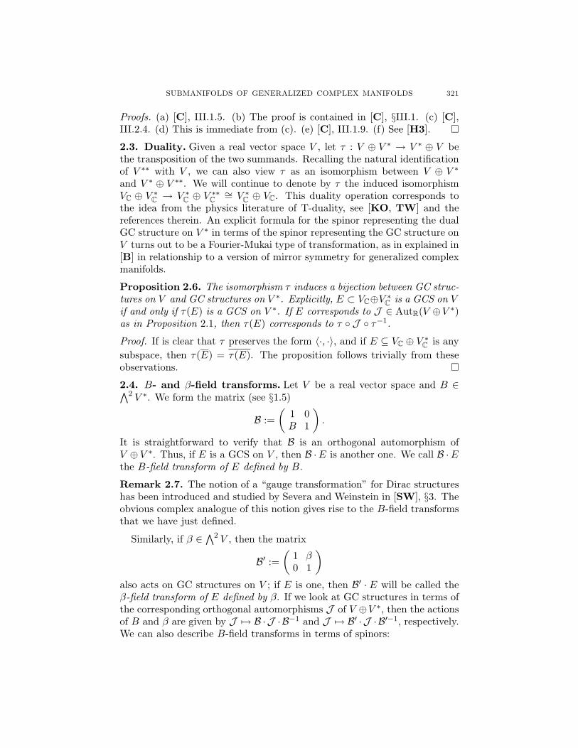


![Geometry of Lagrangian submanifolds related to ...ohnita/2014/BeamerICMSC-RCSOhnita.pdf · [Submanifolds in Riemannian manifolds] (Higher dimensional generalization of curves and](https://static.documents.pub/doc/80x56/5edc153fad6a402d66669985/geometry-of-lagrangian-submanifolds-related-to-ohnita2014beamericmsc-submanifolds.jpg)


