SUBMITTING TO IEEE TRANSACTIONS ON MEDICAL...

SUBMITTING TO IEEE TRANSACTIONS ON MEDICAL IMAGING 1

Automatic Detection of Regional Heart

Rejection in USPIO-Enhanced MRI

Hsun-Hsien Chang, Jose M. F. Moura,Fellow, IEEE,

Yijen L. Wu, and Chien Ho

Abstract

Contrast-enhanced magnetic resonance imaging (MRI) is useful to study the infiltration of cells

in vivo. This research adopts ultrasmall superparamagnetic iron oxide (USPIO) particles as contrast

agents. USPIO particles administered intravenously can beendocytosed by circulating immune cells, in

particular, macrophages. Hence, macrophages are labeled with USPIO particles. When a transplanted

heart undergoes rejection, immune cells will infiltrate theallograft. Imaged by T∗2-weighted MRI, USPIO-

labeled macrophages display dark pixel intensities. Detecting these labeled cells in the image facilitates

the identification of acute heart rejection.

This paper develops a classifier to detect the presence of USPIO-labeled macrophages in the

myocardium in the framework of spectral graph theory. First, we describe a USPIO-enhanced heart

image with a graph. Classification becomes equivalent to partitioning the graph into two disjoint

subgraphs. We use the Cheeger constant of the graph as an objective functional to derive the classifier. We

represent the classifier as a linear combination of basis functions given from the spectral analysis of the

graph Laplacian. Minimization of the Cheeger constant based functional leads to the optimal classifier.

Experimental results and comparisons with other methods suggest the feasibility of our approach to

study the rejection of hearts imaged by USPIO-enhanced MRI.

Index Terms

Cardiac magnetic resonance imaging (cardiac MRI), USPIO-enhanced MRI, contrast agents, acute

heart rejection, spectral graph theory, Cheeger constant,graph cut, graph Laplacian, classification,

classifier.

This work was supported by National Institute of Health grants R01EB/AI-00318 and P41EB001977.

H. H. Chang and J. M. F. Moura are with the Department of Electrical and Computer Engineering, Carnegie Mellon University,

5000 Forbes Ave., Pittsburgh, PA 15213, USA (email: [email protected]; [email protected]).

Y. L. Wu and C. Ho are with the Department of Biological Sciences and the Pittsburgh NMR Center for Biomedical Research,

Carnegie Mellon University, Mellon Institute, 4400 Fifth Ave., Pittsburgh, PA 15213, USA.


I. INTRODUCTION

Heart failure is a major public health crisis in the United States. It is the leading cause of

death and hospitalization in this country. For many patients with end-stage heart failure, heart

transplantation may be the only viable treatment option. Physicians typically assess for cardiac

rejection by performing frequent endomyocardial biopsies. Using biopsy samples, cardiologists

monitor immune cell infiltration and other pathological characteristics of rejection. However,

biopsies are invasive procedures that are subject to patient risk. In addition, due to limited

sampling, biopsies may not detect focal areas of rejection.

Cellular magnetic resonance imaging (MRI) is a useful tool to non-invasively monitor the

migration and localization of cells in the whole heartin vivo [1]. This imaging modality relies

on extrinsic contrast agents, such as ultrasmall superparamagnetic iron oxide (USPIO) particles.

The superior relaxivity of USPIO particles reduces signal emission in T∗2-weighted MRI [2].

In other words, the signal attenuation created in T∗2-weighted MR images localizes the cells

containing a significant number of USPIO particles.

Mammalian cells can be labeled with MRI contrast agents either ex vivoor in vivo. In the

ex vivo method, specific types of cells are isolated, labeled with contrast agents in culture,

and then reintroduced.In vivo method, contrast agents are administered intravenously.In vivo

labeling is effective for cells that can phagocytose or endocytose the contrast agents, and can be

conveniently applied in the clinical studies. We adoptin vivo labeling in this study.

After USPIO particles are administered, circulating macrophages can endocytose USPIO par-

ticles and become USPIO-labeled macrophages. When rejection occurs, the labeled macrophages

migrate to the rejecting tissue. Imaging the transplant by T∗2-weighted MRI, dark pixels represent

the infiltration of macrophages labeled by USPIO particles and identify the rejecting sites [3], [4].

For example, Figure 1 shows the left ventricular image of a rejecting cardiac allograft, where the

darker signal intensities in the myocardium reveal the presence of USPIO-labeled cells, leading

to the detection of the macrophage accumulation. To identify such regions, the first task is to

classify the USPIO-labeled dark pixels in the image.

The usual method to classify USPIO-labeled pixels is manualclassification [4]–[7], or simple

thresholding of the image. Manual classification requires cardiologists to scrutinize the entire

image to determine the location of the USPIO-labeled pixels. Manual classification is labor-


Fig. 1. A USPIO-enhanced cardiac MR image where the dark pixels are segmented. The dark pixels correspond to the locations

of USPIO-labeled abnormal cells.

intensive and operator dependent. In addition, the noise introduced during the imaging, the blur

induced by cardiac motion, and the partial volume effect make dark and bright pixels difficult

to distinguish. Thresholding the intensities is the simplest algorithm to classify USPIO-labeled

pixels; however, this method cannot handle noise. Another drawback of thresholding is that the

operator has to adjust the threshold values, which may introduce inconsistent recordings. To

reduce the labor involved with manual classification, to make the process robust to noise, and

to achieve consistent results, we propose to develop an automatic algorithm for classification of

USPIO-labeled pixels.

To design an automatic classification algorithm, we face thefollowing challenges:

1) Macrophages accumulate in multiple regions without known pattern. For example, Figure 1

displays a rejecting heart where the boundaries of macrophage accumulation are manually

determined. We can see that the macrophage spread randomly throughout the myocardium.

Since there is no model describing how macrophages infiltrate, the algorithm will rely

solely on the MRI data.

2) Due to noise and cardiac motion, the boundaries between the dark and bright pixels are

diffuse and hard to distinguish; as such, any classificationalgorithm has to be robust to

noise.

3) There are a large number of pixels in the myocardium. For instance, the heart shown in

Figure 1 has more than 2500 myocardial pixels. This means that we have to classify more


than 2500 pixels, which may involve estimating a large number of parameters. To avoid

estimating too many parameters and design the classification algorithm in a tractable way,

we transform the problem into another one that expresses theclassifier in terms of a small

number of parameters.

4) There are two types of classifiers for our design: supervised and unsupervised. Supervised

classifiers need human operators to label a subset of the pixels. The classifiers then

automatically propagate the human labels to the remaining pixels. However, the human

knowledge might be unreliable, so the classification results are sensitive to operators. To

avoid the classification inconsistency related to operatordependence, the classifier will be

unsupervised.

A. Overview of Our Approach

We formulate the task of classifying USPIO-labeled regionsas a problem of graph partition-

ing [8]. Given a heart image, the first step is to represent themyocardium as a graph. We treat all

the myocardial pixels as the vertices of a graph, and prescribe a way to assign edges connecting

the vertices. Graph partitioning is a method that separatesthe graph into disconnected subgraphs,

for example, one representing the classified USPIO-labeledregion and the other representing the

unlabeled region of the myocardium. The goal in graph partitioning is to find a small as possible

subset of edges whose removal will separate out a large as possible subset of vertices. In graph

theory terminology, the subset of edges that disjoins the graph is called acut, and the measure

to compare partitioned subsets of vertices is thevolume. Graph partitioning finds theminimal

ratio of the cut to the volume, which is called theisoperimetric numberand is also known as the

Cheeger constant[9] of the graph. Evaluating the Cheeger constant will determine the optimal

edge cut.

The determination of the Cheeger constant, and hence of the optimal edge cut, is a combinato-

rial problem. We can enumerate all the possible combinations of two subgraphs partitioning the

original graph, and then choose the combination with the smallest cut-to-volume ratio. However,

when the number of vertices is very large, the enumeration approach is infeasible. To circumvent

this obstacle, we adopt an optimization framework. We introduce a classifier, or a classification

function, that determines to which class each pixel belongs, and derive from the Cheeger constant

an objective functional to be minimized with respect to the classifier. The minimization leads to


the optimal classification.

If there is a complete set of basis functions on the graph, we can represent the classifier

by a linear combination of the basis. There are various ways to obtain the basis functions,

e.g., using the Laplacian operator [10], the diffusion kernel [11], or the Hessian eigenmap [12].

Among these, we choose the Laplacian. The spectrum of the Laplacian operator has been used

to obtain upper and lower bounds on the Cheeger constant [8];we utilize these bounds to

derive our objective functional. The eigenfunctions of theLaplacian form a basis of the Hilbert

space of square integrable functions defined on the graph. Thus, we express the classifier as

a linear combination of the Laplacian eigenfunctions. Since the basis is known, the optimal

classifier is determined by the linear coefficients in the combination. The classifier can be

further approximated as a linear combination of only themost relevantbasis functions. The

approximation reduces significantly the problem of lookingfor a large number of coefficients to

estimating only a few of them. Once we determine the optimal coefficients, the optimal classifier

automatically partitions the myocardial image into USPIO-labeled and unlabeled parts.

B. Paper Organization

This paper extends our work briefly presented in [13]. The organization of this paper is

as follows. Section II describes how we represent a heart image by a graph and introduces the

Cheeger constant for graph partitioning. Section III details the optimal classification algorithm in

the framework of spectral graph theory. In Section IV, we describe the algorithm implementation

and show our experimental results for USPIO-enhanced MRI data on heart transplants. We

contrast the proposed method with the results of manual classification, thresholding, another

graph based algorithm, and the level set approach. Finally,Section V concludes this paper.

II. GRAPH REPRESENTATION ANDGRAPH PARTITIONING

For a given USPIO-enhanced MR image, we first segment the leftventricle and remove

artifacts. Then, the myocardial pixels are arranged into a single column vector indexed by a set

of integersI = {1, 2, · · · , Nmyo}, whereNmyo is the number of myocardial pixels. The image

intensity becomes a functionf : I 7→ R. We next describe how to represent the image as a

graph.


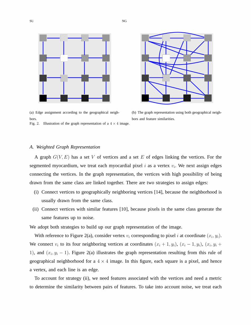
(a) Edge assignment according to the geographical neigh-

bors.

(b) The graph representation using both geographical neigh-

bors and feature similarities.Fig. 2. Illustration of the graph representation of a4× 4 image.

A. Weighted Graph Representation

A graph G(V, E) has a setV of vertices and a setE of edges linking the vertices. For the

segmented myocardium, we treat each myocardial pixeli as a vertexvi. We next assign edges

connecting the vertices. In the graph representation, the vertices with high possibility of being

drawn from the same class are linked together. There are two strategies to assign edges:

(i) Connect vertices to geographically neighboring vertices [14], because the neighborhood is

usually drawn from the same class.

(ii) Connect vertices with similar features [10], because pixels in the same class generate the

same features up to noise.

We adopt both strategies to build up our graph representation of the image.

With reference to Figure 2(a), consider vertexvi corresponding to pixeli at coordinate(xi, yi).

We connectvi to its four neighboring vertices at coordinates(xi + 1, yi), (xi − 1, yi), (xi, yi +

1), and (xi, yi − 1). Figure 2(a) illustrates the graph representation resulting from this rule of

geographical neighborhood for a4× 4 image. In this figure, each square is a pixel, and hence

a vertex, and each line is an edge.

To account for strategy (ii), we need features associated with the vertices and need a metric

to determine the similarity between pairs of features. To take into account noise, we treat each


pixel as a random variable and adopt theMahalanobis distance, [15], as similarity measure. We

stack aNw ×Nw block of pixels centered at pixeli into a column vectorxi, which we treat as

the feature vector for the vertexvi. The Mahalanobis distanceρij between the featuresxi, xj of

verticesvi, vj is, see [15],

ρij =√

(xi − xj)T Σ−1i,j (xi − xj) , (1)

where Σi,j is the covariance matrix betweenxi and xj. When the distanceρij is below a

predetermined thresholdτρ, the verticesvi, vj are connected by an edge; otherwise, they are

disconnected. Figure 2(b) shows the final graph representation of the4×4 image example using

both geographical neighbors and feature similarities.

In graph theory, we usually considerweightedgraphs [8]. Since not all connected pairs of

vertices have the same distances, we capture this fact by using a weight function on the edges.

We adopt a Gaussian kernel, suggested by Belkin and Niyogi [10] and used also by Coifman

et al. [11], to compute the weightsWij on edgeseij connecting verticesvi andvj :

Wij =

exp(

−ρ2

ij

σ2

)

, if there is edgeeij

0 , if no edgeeij

, (2)

whereσ is the Gaussian kernel parameter. The largerσ is, the more weight far-away vertices will

exert on the weighted graph. The weightWij is large when the features of two linked vertices

vi, vj are similar.

The weighted graph is equivalently represented by itsNmyo×Nmyo weighted adjacency matrix

W whose elementsWij are the edge weights in equation (2). Note that the matrixW has a

zero diagonal because we do not allow the vertices to be self-connected; it is symmetric since

Wij = Wji.

B. Graph Partitioning and the Cheeger Constant

Classification is to partition the set of pixels into disjoint sets. In graph terms, we divide the

graphG(V, E) into two subgraphs. The task is to find out a subsetE0 of edges, called anedge cut

such that removing this cut separates the graphG(V, E) into two disconnected subgraphsG1 =

(V1, E1) andG2 = (V2, E2), whereV = V1 ∪ V2, ∅ = V1 ∩ V2, andE = E0 ∪ E1 ∪ E2. Taking

the example of the4× 4 image again, the dotted edges shown in Figure 3(a) assemble an edge


(a) Dotted edges assemble an edge cut. (b) Removal of the edge cut partitions the graph.

Fig. 3. Conceptualization of an edge cut associated to the4× 4 image in Figure 2(b).

cut for the graph. The removal of this edge cut partitions thegraph into two parts as shown in

Figure 3(b).

In the framework of spectral graph theory [8], we define anoptimal edge cut by looking for

the Cheeger constantΓ(V1) of the graph,

Γ(V1) = minV1⊂V

|E0(V1, V2)|vol(V1)

, (3)

assuming that vol(V1) ≤ vol(V2). In equation (3),|E0(V1, V2)| is the sum of the edge weights in

the cutE0:

|E0(V1, V2)| =∑

vi∈V1,vj∈V2

Wij . (4)

The volume vol(V1) of V1 is defined as the sum of the vertex degrees inV1:

vol(V1) =∑

vi∈V1

di , (5)

where the degreedi of the vertexvi is defined as

di =∑

vj∈V

Wij . (6)

To denote the partition of the graph vertices, we introduce an indicator vectorχ for V1 whose

elements are defined as

χi =

1, if vi ∈ V1

0, if vi ∈ V2

. (7)


In Appendix I, we derive the Cheeger constant in terms of the indicator vectorχ:

Γ(χ) = minχ

χTLχ

χTd, (8)

whereL is the graph Laplacian defined in (48) andd is the vector collecting vertex degrees.

The optimal graph partitioning corresponds to the optimal indicator vector

χ = argminχ

χTLχ

χTd. (9)

C. Objective Functional for Cheeger Constant

In equation (8), the minimization of the cut-to-volume ratio is equivalent to minimizing an

objective functional

Q(χ) = χTLχ− βχT

d , (10)

whereβ is the weight. The objectiveQ(χ) is convex, because the graph LaplacianL is positive

semidefinite, see Appendix I. In addition, the second term0 ≤ χTd ≤ vol(V ) is finite, so the

minimizer χ exists.

Since at each vertex the indicator is either 1 or 0, see equation (7), there are2Nmyo candidate

indicator vectors. When the number of pixelsNmyo in the myocardium is large, it is not compu-

tationally feasible to minimize the objective by enumerating all the candidate indicator vectors.

The next section proposes a novel algorithm to avoid this combinatorial problem.

III. OPTIMAL CLASSIFICATION ALGORITHM

This section develops the optimal classifier that utilizes the Cheeger constant.

A. Spectral Analysis of the Graph LaplacianL

The spectral decomposition of the graph LaplacianL, which is defined in equation (48),

gives the eigenvalues{λn}Nmyon=1 and eigenfunctions{φ(n)}Nmyo

n=1 . By convention, we index the

eigenvalues in ascending order. Because the LaplacianL is symmetric and positive semidefinite,

its spectrum{λn} is real and nonnegative and its rank isNmyo− 1. In the framework of spectral

graph theory [8], the eigenfunctions{φ(n)} assemble a complete set and span the Hilbert space of

square integrable functions on the graph. Hence, we can express any square integrable function on

the graph as a linear combination of the basis functions{φ(n)}. The domain of the eigenfunctions


are vertices, so the eigenfunctions{φ(n)} are discrete and are represented by vectors. We note that

both the eigenfunctions and the vertices are indexed by the set of integersI = {1, 2, · · · , Nmyo}.Eigenfunctionφ(n) is the vector

φ(n) = [φ(n)1 , φ

(n)2 , · · · , φ(n)

Nmyo]T . (11)

We list here the properties of the spectrum of the Laplacian (see see [8] for additional details)

that will be utilized to develop the classification algorithm:

1) For aconnectedgraph, there is only one zero eigenvalueλ1, and the spectrum is

0 = λ1 < λ2 ≤ · · · ≤ λNmyo . (12)

The first eigenvectorφ(1) is constant, i.e.,

φ(1) = α[1, 1, · · · , 1]T , (13)

whereα = 1√Nmyo

is the normalization factor forφ(1).

2) The eigenvectorsφ(n) with nonzero eigenvalues have zero averages,

Nmyo∑

i=1

φ(n)i = 0 . (14)

The low order eigenvectors correspond to low frequency harmonics.

3) For aconnectedgraph, the Cheeger constantΓ defined by (8) is upper and lower bounded

by the following inequality:1

2λ2 ≤ Γ <

√

2λ2 . (15)

Due to the edge assignment strategy of geographical neighborhood, see Section II, our graphs

representing the heart images are connected. Therefore, the spectral properties in (12) and (15)

hold in our case, besides the property (14) that holds in general.

B. Expression of Classifier

We now consider the graphG(V, E) that describes the myocardium in an MRI heart image.

The classifierc partitioning the graph vertex setV into two classesV1 andV2 is defined as

ci =

1, if vi ∈ V1

−1, if vi ∈ V2

. (16)


Utilizing the spectral graph analysis, we express the classifier in terms of the eigen-basis{φ(n)}

c =

Nmyo∑

n=1

anφ(n) = Φa , (17)

wherean are the coordinates of the eigen representation,a = [a1, a2, · · · , aNmyo]T is a vector

stacking the coefficients, andΦ is a matrix collecting the eigen-basis

Φ =[

φ(1), φ(2), · · · , φ(Nmyo)]

. (18)

The design of the optimal classifierc becomes now the problem of estimating the linear com-

bination coefficientsan.

C. Objective Functional for Classification

In equation (8), the Cheeger constant is expressed in terms of the set indicator vectorχ that

takes 0 or 1 values. On the other hand, the classifierc defined in (16) takes±1 values. We relate

χ andc by the standard Heaviside functionH(x) defined by

H(x) =

1, if x ≥ 0

0, if x < 0. (19)

Hence, the indicator vectorχ = [χ1, χ2, · · · , χNmyo]T for the setV1 is given by

χi = H(ci) . (20)

In equation (20), the indicatorχ is a function of the classifierc using the Heaviside functionH.

Furthermore, by (17), the classifierc is parametrized by the coefficient vectora, so the objective

functionalQ is parametrized by this vectora, i.e.,

Q(a) = χ(c(a))TLχ(c(a))− βχ(c(a))T

d . (21)

Minimizing Q with respect toa gives the optimal coefficient vectora, which leads to the optimal

classifierc = Φa. Using eigen-basis to represent the classifier transforms the problem of the

combinatorial optimization in (10) to estimating the real-valued coefficient vectora in (21).

To avoid estimating too many parameters, we relax the classification function to a smooth

function, which simply requires the firstp harmonics in its expression in terms of the eigen-

basis. The classifierc is now

c =

p∑

n=1

anφ(n) = Φa , (22)


wherea = [a1, a2, · · · , ap]T andΦ =

[

φ(1), φ(2), · · · , φ(p)]

. The estimation of theNmyo parameters

in (17) is reduced to thep ≪ Nmyo parameters in (22). As long asp is chosen small enough,

the latter is more numerically tractable than the former.

Another concern in the objective functional (10) is the weighting parameterβ. If we knew

the Cheeger constantΓ, we could setβ = Γ and the objective function would be

Q(χ) = χTLχ− ΓχT

d . (23)

The solution would correspond toQ(χ) = 0, see (8). However, we cannot setβ = Γ beforehand,

since the Cheeger constantΓ(χ) is dependent on the unknown optimal indicator vectorχ.

We can reasonably predetermineβ by using one of the spectral properties of the graph

Laplacian: The upper and lower bounds of the Cheeger constant are related to the first nonzero

eigenvalueλ2 of the graph Laplacian, see equation (15). The bounds restrain the range of values

for the weightβ. For simplicity, we setβ to the average of the Cheeger constant’s upper and

lower bounds,

β =1

2

(

1

2λ2 +

√

2λ2

)

. (24)

D. Minimization Algorithm

Taking the gradient ofQ(a), we obtain

∂Q

∂a= 2

(

∂χT

∂a

)

Lχ− β

(

∂χT

∂a

)

d . (25)

In equation (25), the computation of(

∂χT

∂a

)

is

(

∂χT

∂a

)

=

[

∂χ1

∂a,∂χ2

∂a, · · · , ∂χNmyo

∂a

]

(26)

=

∂χ1

∂a1

∂χ2

∂a1

· · · ∂χNmyo

∂a1

...... · · · ...

∂χ1

∂ap

∂χ2

∂ap· · · ∂χNmyo

∂ap

. (27)


Using the chain rule, the entries(

∂χT

∂a

)

mnare

(

∂χT

∂a

)

mn

=∂χn

∂am

(28)

=∂χn

∂cn

∂cn

∂am

(29)

= δ(cn)∂

∑p

j=1 ajφ(j)n

∂am

(30)

= δ(cn)φ(m)n . (31)

In (30), δ(x) is the delta (generalized) function defined as the derivative of the Heaviside

functionH(x).

To facilitate numerical implementation, we use the regularized Heaviside functionHǫ and the

regularized delta functionδǫ; they are defined, respectively, as

Hǫ(x) =1

2

[

1 +2

πarctan

(x

ǫ

)

]

, (32)

and

δǫ(x) =dHǫ(x)

dx=

1

π

(

ǫ

ǫ2 + x2

)

. (33)

Replaced with the regularized delta function, the explicitexpression of(

∂χT

∂a

)

is

(

∂χT

∂a

)

=

δǫ(c1)φ(1)1 δǫ(c2)φ

(1)2 · · · δǫ(cNmyo)φ

(1)Nmyo

...... · · · ...

δǫ(c1)φ(p)1 δǫ(c2)φ

(p)2 · · · δǫ(cNmyo)φ

(p)Nmyo

(34)

= ΦT ∆ , (35)

where we define

∆ = diag(

δǫ(c1), δǫ(c2), · · · , δǫ(cNmyo))

. (36)

Substituting (35) into (25), the gradient of the objective has the compact form

∂Q

∂a= 2ΦT ∆Lχ− βΦT ∆d . (37)

The optimal coefficient vectora is obtained by looking for∂Q

∂a= 0. We have to solve the

minimization numerically, because the unknowna is inside the matrix∆ and the vectorχ. We


adopt the gradient descent algorithm to iteratively find thesolution a. The classifierc is then

determined by

c = Φa . (38)

The vertices with indicatorsχi = H(ci) = 1 correspond to classV1 and 0 correspond to class

V2. To select the desired USPIO-labeled regions, the operatorsimply chooses one of the two

classes.

E. Algorithm Summary

There are two major algorithms in the classifier development: graph representation and clas-

sification. We summarize them in the Algorithms 1 and 2, respectively.

Algorithm 1 The graph representation algorithm1: procedure GRAPHREP(f ) ⊲ Load the imagef

2: Segment the left ventricle

3: Index all the myocardial pixels by a set of integersI = {1, · · · , Nmyo}4: Initialize W as anNmyo×Nmyo zero matrix

5: for all i 6= j ∈ I do

6: Compute Mahalanobis distanceρij by (1)

7: if ρij < τρ or i, j are geographical neighborsthen

8: Wij ← Compute edge weightWij by (2)

9: end if

10: end for

11: return W

12: end procedure

IV. EXPERIMENTS

This section presents the performance of the classifier withexperimentally obtained USPIO-

enhanced MRI of phantoms and of transplanted rat hearts. We implement our algorithm with

MATLAB R© on a computer with a 3 GHz CPU and 1 GB RAM. After data acquisition, we

normalize the heart image intensities to range from 0 to 1 andmanually segment the left ventricle.


Algorithm 2 The classification algorithm1: procedure CLASSIFIER(W)

2: Compute graph LaplacianL by (48)

3: EigendecomposeL to obtain{λn} and{φ(n)}4: Compute coefficientβ by (24)

5: Initialize classifier coefficienta = 1 and objectiveQ =∞6: repeat

7: c← Compute classifierc by (22)

8: χ← Compute indicator vectorχ by (20)

9: Q← Compute objectiveQ by (21)

10: a← Computea− ∂Q

∂aby (37)

11: until ∂Q

∂a= 0

12: return χ

13: end procedure

Classifier Setting:There are several parameters needed for running the classifier; their values

are described in the following.

• Each vertexvi is associated with aNw×Nw block of pixels centered at pixeli for computing

the Mahalanobis distance, see Section II-A. We setNw = 3. If Nw is 1, noise is not taken

into account. IfNw is large, the graph takes better account of the impact of the noise but the

computational time for constructing the graph increases. Our choice ofNw is a compromise

between these two issues.

• To derive the image graph, we setσ = 0.1 when computing the edge weights in (2). This

choice ofσ is suggested by Shi and Malik [14], who indicate empiricallythat σ should be

set at10% of the range of the image intensities.

• The parameterǫ for the regularized Heaviside and delta functions in (32) and (33), respec-

tively, is set to0.1. The smaller the parameterǫ is, the sharper these two regularized functions

are. Forǫ = 0.1, the regularized functions are a good approximation to the standard ones.

• To determine the numberp of lowest order eigenfunctions used to represent the classifier

c, we tested values ofp from 5 to 20. We obtain the best results forp = 16.


• To reach the minimum of the objective functional, we solve∂Q

∂a= 0 recursively. We stop

the iterative process when the norm of the gradient is smaller than 10−4 or when the

minimization reaches200 iterations. This number of iterations led to convergence inall

of our experiments, although, in most cases, we observed convergence within the first100

iterations.

A. Phantom Study

We design a phantom to investigate how our algorithm performs under various contrast-to-noise

ratios (CNRs). The phantom sample consists of three tubes that contain different concentration

of iron-oxide particles and that are surrounded by water. Weimaged the phantom with a Bruker

AVANCE DRX 4.7-Tesla system with a5.5-cm home-built surface coil. To generate CNRs from

low to high, we run three series of scans:

• Series 1: fixed repetition time (TR) =1000 ms and number of signal averages (NEX) =2;

varied echo time (TE) =3 to 15 ms.

• Series 2: fixed TR =500 ms and TE =5 ms; varied NEX =1 to 12.

• Series 3: fixed TE =5 ms and NEX =2; varied TR =300 to 1500 ms.

To compute CNR of an image, we begin with calculating signal-to-noise ratios (SNRs) of

USPIO-labeled and -unlabeled regions:

SNRlab =average signal of USPIO-labeled regionsstandard deviation of background noise

, (39)

SNRunlab =average signal of unlabeled regions

standard deviation of background noise. (40)

Then, CNR is determined as

CNR = |SNRlab− SNRunlab| . (41)

The percentage of misclassified pixels is the criterion to evaluate the performance of the classifier.

Figure 4 plots the percentage error versus CNR for the three series of scans. With reference to

Figures 4(a), 4(b) and 4(c), the proposed algorithm achieves perfect classification when the CNR

is larger than6, but the error increases considerably when the CNR is below5. This phantom

study suggests that the MRI protocol should be designed to reach CNR =6 or above so that the

classifier can perform without errors.


TABLE I

SNRAND CNR VERSUSPOD.

POD3 POD4 POD5 POD6 POD7

SNR of USPIO-unlabeled myocardium 24.87 20.79 16.77 25.36 21.71

SNR of USPIO-labeled myocardium 12.89 13.11 9.71 11.81 10.38

CNR of USPIO-enhanced myocardium11.98 7.68 7.06 13.55 11.33

B. Cardiac Rejection Study

USPIO-Enhanced MRI of Heart Transplants: We have studied the acute cardiac rejection

of transplanted hearts using our heterotopic working rat heart model. All rats were male inbred

Brown Norway (BN; RT1n) and Dark Agouti (DA; RT1a), obtainedfrom Harlan (Indianapolis,

IN), with body weight between0.18 and0.23 kg each. We transplanted DA hearts to BN hosts.

Home-made dextran-coated USPIO particles [3] of27 nm in size were administered intravenously

one day prior to MRI with a dosage of4.5 mg per kg bodyweight.

To investigate the acute cardiac progression, we have imaged five different transplanted rat

hearts on post-operation days (PODs) 3, 4, 5, 6, and 7, individually. In our heterotopic rat cardiac

transplant model, mild acute rejection begins on POD 3, progresses to moderate rejection on

PODs 4 and 5, severe and very severe rejection on PODs 6 and 7, respectively [4]. Each heart

was imaged with ten short-axis slices covering the entire left ventricle. In vivo imaging was

carried out on the same machine in the phantom study. T∗2-weighted imaging was acquired with

gradient echo recall sequence. Respiratory as well as electrocardiogram gating is used to control

respiratory and heart motion artifacts for MR imaging. The MRI protocol has the following

parameters: TR = one cardiac cycle (about180 ms); TE = 8 to 10 ms; NEX = 4; flip angle

= 90◦; field of view = 3 to 4 cm; slice thickness =1 to 1.5 mm; in-plane resolution =117 to

156 µm. The MRI protocol is optimized to guarantee that the classifier works in a valid CNR

range. Table I summarizes the SNRs and CNRs in various POD data. The CNRs are all greater

than6, which was the threshold for the classifier to achieve perfect classification in the phantom

study.

Automatic Classification Results: Figure 5(a) shows different transplanted hearts imaged

on PODs 3, 4, 5, 6, and 7. Each image is the sixth slice out of tenacquired slices for the


heart; its location in the heart corresponds to the equator of the left ventricle. Then, we apply

our classification algorithm to the images. Figure 5(b) shows the detected USPIO-labeled areas

denoted by red (darker pixels). Unlike time-consuming manual classification, our algorithm takes

less than three minutes to determine the regional macrophage accumulation for each image.

To take into account the 3D heart, we process slices 3 to 8 out of 10 for the current study.

We do not use the first two and the last two slices because they do not clearly contain the

myocardium. The classifier automatically determines sliceby slice the USPIO-labeled regions

of the heart.

Validation with Manual Classification: Wu et al. [4] have shown that the dark patches in

the MR images are due to those macrophages labeled with USPIOparticles whose presence

is correlated histologically and immunologically with acute cardiac rejection. Since the best

validation option right now is to compare with classification results by a human expert, we treat

manually determined USPIO-labeled pixels as the gold standard. In our data set, we can see

that manual classification of the heart slices is appropriate for all PODs, except POD5, as we

will discuss shortly. Manual classification of all the heartslices at all PODs has been carried out

before running the automatic classification. Figure 5(c) shows the manually classified USPIO-

labeled regions. Our automatically detected regions show good agreement with the manual results

in all slices and PODs, except for POD5. This qualitative validation suggests that our automatic

approach is useful in the study of heart rejection based on USPIO-enhanced MRI data.

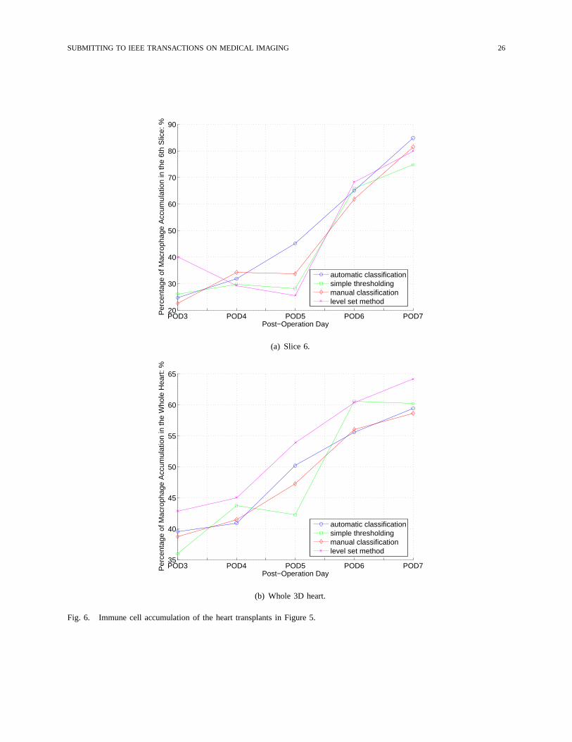
To quantitatively evaluate the quality of the automatic classification, we have compared the

total area of USPIO-labeled regions determined by the classifier and determined manually. In

Figure 6(a), we plot the total macrophage accumulation percentage for slice 6 as a function of

the PODs for the data used in Figure 5. Figure 6(b) shows similar results but for the whole 3D

heart.

To appreciate better how much the classifier deviates from manual classification, we define

the percentage error as

P (ε) =|(automatic USPIO-labeled area)− (manual USPIO-labeled area)|

myocardium area, (42)

which we show in Figure 7(a). Since the noise levels in different slices are not identical, the

classification errors vary from slice to slice. The deviation of the classifier, usually below4%,

shows the very good agreement between the classifier and manual classification for all PODs,


except POD5.

We now consider the discrepancy between the automatic classifier and the manual classification

results in POD5. The five slices in POD5 heart have percentageerrors larger than6%, with one

of them exceeding10%. POD5 data sets are the most challenging among all POD data sets.

This is because POD5 slices are the most noisy, see Table I, and where the macrophages spread

dispersively, as rejection spreads from the periphery of the heart (epicardium) to the whole heart.

With reference to the POD5 image (middle image on the left column) in Figure 5(a), we see

many dark punctate blobs corresponding to the presence of macrophages. Manual selection of

these blobs is challenging to a human operator. By missing many of these, the lines displaying the

manual classification results (percentage area or percentage volume) in Figures 6(a) and 6(b),

respectively, fail to be nondecreasing, showing a dip at POD5. Were this true, the level of

rejection would have decreased from POD4 to POD5, clearly a contradiction, since the animal

models were not treated and rejection becomes more prevalent as time progresses. In contrast,

the corresponding plot lines for the classifier are monotonic—while they track well the manual

classification results everywhere else, they deviate from the dip at POD5.

Comparisons with Other Classification Approaches:In addition to manual classification,

simple thresholding is the common automatic method used forclassification of USPIO-labeled

regions. Figure 8(a) shows the classification results obtained by thresholding the images in Fig-

ure 5(a). Figures 6(a) and 6(b) also plot the macrophage accumulation curves using thresholding.

The error analysis of the thresholding classification is shown in Figure 7(b) using the same

definition for percentage deviation in (42). Although the classification results by our classifier

and by thresholding shown in Figures 5(b) and 8(a), respectively, are visually indistinguishable,

the quantitative error analysis shown in Figure 7(b) demonstrates that the thresholding method

has higher error rates in most slices than automatic classifier. Further, thresholding is not robust,

with error rates that can range from0.5% to 18.5%, usually with error rates larger than6%.

Thresholding is prone to inconsistency because of the subjectivity in choosing the thresholds

and because it does not account for the noise and motion blurring the images.

We provide another comparison by contrasting our algorithmwith an alternative classifier,

namely, theisoperimetric partitioningalgorithm proposed by Grady and Schwartz [16]. The

isoperimetric algorithm uses also a graph representation,which includes a geographical neigh-

borhood only, not taking into account the noise for edge weights, as in our approach. The


isoperimetric algorithm tries to minimize the objective functioncTLc, wherec is the real-valued

classification function andL is the graph Laplacian. The minimization is equivalent to solving

the linear systemLc = 0. We applied this method to the images in Figure 5(a). The classification

results are shown in Figure 8(b). Comparing these results with the manual classification results

in Figure 5(c), we conclude that the isoperimetric partitioning algorithm fails completely on this

data set. The problems with this method are twofold. First, the objective function captures the

edge cut but ignores the volume enclosed by the edge cut. Thiscontrasts with our functional,

the Cheeger constant, that captures faithfully the goal of minimizing the cut-to-volume ratio.

Second, although the desired classifier of the isoperimetric partitioning is a binary function, the

actual classifier it considers is a relaxed real-valued function. Our approach addresses this issue

via the Heaviside function.

The final comparison is between our proposed method and thelevel setapproach [17], [18],

which has been applied successfully to segment the heart stuctures [19]. The level set method

finds automatically contours that are the zero level of a level set function defined on the image

and that are boundaries between USPIO-labeled and -unlabeled pixels. The optimal level set

is obtained to meet the desired requirements: (i) the regions inside and outside the contours

have distinct statistical models, (ii) the contours capture sharp edges, and (iii) the contours are

as smooth as possible. Finally, we can classify the pixels enclosed by the optimal contours

as USPIO-labeled areas. The experimental results using thelevel set approach are shown in

Figures 7(c) and 8(c). In the heart images, macrophages are present not only in large regions

but also in small blobs with irregular shapes whose edges do not provide strong forces to attract

contours. The contour evolution tends to pass small blobs and capture large continua, leading to

more misclassification than our proposed method.

The performance of our proposed classifier may be affected when artifacts are present in the

MR images. Our method establishes the graphical representation of the images from geographical

and intensity similarities among pixels. If a myocardial region has hypointensity due to artifacts,

its intensity features are similar to those of USPIO-labeled pixels and the classifier will have a

hard time to distinguish correctly between the artifacts and the USPIO-labeled regions. Although

artifacts were not present in our data sets, the operator mayneed to invoke an artifact removal

algorithm before running our classifier.

The classifier presented in this paper performs binary classification of the myocardial pixels


and then determines the rejection severity by counting the number of pixels per volume involved

in USPIO-labeling. Since macrophage infiltration depends on the rejection severity, less for mild

rejection, more for severe rejection, the USPIO-labeled rejecting tissue does not contribute the

same levels of MR signals. In future work, we will extend thisclassifier to handle multiple

classes to provide an integrated mechanism to measure rejection severity.

V. CONCLUSIONS

This paper develops an automatic algorithm to classify regional macrophage accumulation of

allografts imaged by USPIO-enhanced MRI. Automatic classification is desirable. It lightens the

manual work of an expert, prevents inconsistencies resulting from different choices of thresholds

that usually plague classification by human operators, and,by accounting in its design explicitly

for noise, it is robust to noise. The classifier developed in this paper can assist in studying

rejection in heart transplants.

We formulate the classification task as a graph partitioningproblem. We associate to an MR

image a graph where the graph vertices denote pixels and the graph edges connect neighboring

and similar pixels. We treat the classifier as a binary function on the graph. The eigendecom-

position of the graph Laplacian provides a basis to represent the classifier. The binary classifier

is relaxed to a smooth function by linearly combining several low order eigen basis functions.

The optimal classifier is designed to minimize an objective functional derived from the Cheeger

constant of the graph. Our experimental results with USPIO-enhanced MRI data of small animals’

cardiac allografts undergoing rejection show that the Cheeger graph partitioning based classifier

can determine accurately the regions of macrophage infiltration. These experiments show that

it presents better performance than other methods like the commonly used thresholding, the

isoperimetric algorithm, and a level set based approach.

APPENDIX I

EXPRESSION OF THECHEEGER CONSTANTΓ IN TERMS OF THE INDICATOR VECTORχ

We can rewrite the vertex degreedi, see (6), by considering the verticesvj in eitherV1 or V2;

i.e.,

di =∑

vj∈V1

Wij +∑

vj∈V2

Wij . (43)


Assuming that the vertexvi is in V1, the second term in equation (43) is the contribution ofvi

made to the edge cut|E0(V1, V2)|. Taking into account all the vertices inV1, we have the edge

cut

|E0(V1, V2)| =∑

vi∈V1

∑

vj∈V2

Wij (44)

=∑

vi∈V1

di −∑

vj∈V1

Wij

. (45)

To write equation (45) in a more compact form, we use the indicator vectorχ for V1, defined

in (7). It follows that the edge cut (45) is

|E0(V1, V2)| = χTDχ− χT

Wχ (46)

= χTLχ , (47)

whereD = diag(

d1, d2, · · · , dNmyo

)

is a diagonal matrix of vertex degrees, and

L = D−W (48)

is the Laplacian of the graph, see [8]. BecauseD is diagonal andW is symmetric,L is symmetric.

Further,L is positive semidefinite since the row sums ofL are zeros.

Using the indicator vectorχ, we express the volume vol(V1) as

vol(V1) =∑

vi∈V1

di = χTd , (49)

whered is the column vector collecting all the vertex degrees. Replacing (47) and (49) into the

Cheeger constant (3), we write the Cheeger constant in termsof the indicator vectorχ:

Γ(χ) = minχ

χTLχ

χTd. (50)

REFERENCES

[1] C. Ho and T. K. Hitchens, “A non-invasive approach to detecting organ rejection by MRI: monitoring the accumulation

of immune celss at the transplanted organ,”Current Pharmaceutical Biotechnology, vol. 5, pp. 551–566, December 2004.

[2] R. Weissleder, G. Elizondo, J. Wittenberg, C. A. Rabito,H. H. Bengele, and L. Josephson, “Ultrasmall superparamagnetic

iron oxide: Characterization of a new class of contrast agents for MR imaging,”Radiology, vol. 175, pp. 489–493, May

1990.

[3] S. Kanno, Y. L. Wu, P. C. Lee, S. J. Dodd, M. Williams, B. P. Griffith, and C. Ho, “Macrophage accumulation associated

with rat cardiac allograft rejection detected by magnetic resonance imaging with ultrasmall superparamagnetic iron oxide

particles,”Circulation, vol. 104, pp. 934–938, August 2001.


[4] Y. L. Wu, Q. Ye, L. M. Foley, T. K. Hitchens, K. Sato, J. B. Williams, and C. Ho, “In situ labeling of immune cells with

iron oxide particles: An approach to detect organ rejectionby cellular MRI,” Proceedings of the National Academy of

Sciences of the United States of America, vol. 103, pp. 1852–1857, February 2006.

[5] M. Hoehn, E. Kustermann, J. Blunk, D. Wiedermann, T. Trapp, S. Wecker, M. Focking, H. Arnold, J. Hescheler, B. K.

Fleischmann, W. Schwindt, and C. Buhrle, “Monitoring of implanted stem cell migrationin vivo: A highly resolvedin

vivo magnetic resonance imaging investigation of experimentalstroke in rats,”Proceedings of the National Academy of

Sciences of the United States of America, vol. 99, pp. 16267–16272, December 2002.

[6] R. A. Trivedi, J.-M. U-King-Im, M. J. Graves, J. J. Cross,J. Horsley, M. J. Goddard, J. N. Skepper, G. Quartey, E. Warburton,

I. Joubert, L. Wang, P. J. Kirkpatrick, J. Brown, and J. H. Gillard, “In vivo detection of macrophages in human carotid

atheroma: temporal dependence of ultrasmall superparamagnetic particles of iron oxide-enhanced MRI,”Stroke, vol. 35,

pp. 1631–1635, July 2004.

[7] M. Sirol, V. Fuster, J. J. Badimon, J. T. Fallon, P. R. Moreno, J.-F. Toussaint, and Z. A. Fayad, “Chronic thrombus

detection with in vivo magnetic resonance imaging and a fibrin-targeted contrast agent,”Circulation, vol. 112, pp. 1594–

1600, November 2005.

[8] F. R. K. Chung, Spectral Graph Theory, vol. 92 of CBMS Regional Conference Series in Mathematics. American

Mathematical Society, 1997.

[9] J. Cheeger, “A lower bound for the smallest eigenvalue ofthe Laplacian,” inProblems in Analysis(R. C. Gunning, ed.),

pp. 195–199, Princeton, NJ: Princeton University Press, 1970.

[10] M. Belkin and P. Niyogi, “Laplacian eigenmaps for dimensionality reduction and data representation,”Neural Computation,

vol. 15, pp. 1373–1396, June 2003.

[11] R. R. Coifman, S. Lafon, A. B. Lee, M. Maggioni, B. Nadler, F. Warner, and S. W. Zucker, “Geometric diffusions as

a tool for harmonic analysis and structure definition of data: Diffusion maps,”Proceedings of the National Academy of

Sciences of the United States of America, vol. 102, pp. 7426–7431, May 2005.

[12] D. L. Donoho and C. Grimes, “Hessian eigenmaps: Locallylinear embedding techniques for high-dimensional data,”

Proceedings of the National Academy of Sciences of the United States of America, vol. 100, pp. 5591–5596, May 2003.

[13] H.-H. Chang, J. M. F. Moura, Y. L. Wu, and C. Ho, “Immune cells detection ofin vivo rejecting hearts in USPIO-enhanced

magnetic resonance imaging,” inProceedings of IEEE International Conference of Engineering in Medicine and Biology

Society, (New York, NY), pp. 1153–1156, August 2006.

[14] J. Shi and J. Malik, “Normalized cuts and image segmentation,” IEEE Transactions on Pattern Analysis and Machine

Intelligence, vol. 22, pp. 888–905, August 2000.

[15] R. O. Duda, P. E. Hart, and D. G. Stork,Pattern Classification. New York, NY: John Wiley & Sons, second ed., 2001.

[16] L. Grady and E. L. Schwartz, “Isoperimetric graph partitioning for image segmentation,”IEEE Transactions on Pattern

Analysis and Machine Intelligence, vol. 28, pp. 469–475, March 2006.

[17] S. Osher and J. A. Sethian, “Fronts propagating with curvature-dependent speed: Algorithms based on Hamilton–Jacobi

formulations,”Journal of Computational Physics, vol. 79, pp. 12–49, November 1988.

[18] J. A. Sethian,Level Set Methods and Fast Marching Methods. New York, NY: Cambridge University Press, second ed.,

1999.

[19] C. Pluempitiwiriyawej, J. M. F. Moura, Y. L. Wu, and C. Ho, “STACS: New active contour scheme for cardiac MR image

segmentation,”IEEE Transactions on Medical Imaging, vol. 24, pp. 593–603, May 2005.


0 5 10 15 200

10

20

30

40

50

60

70

80

90

100

Contrast−to−noise ratio

Per

cent

age

erro

r: %

(a) Varied TE.

0 5 10 15 200

10

20

30

40

50

60

70

80

90

100


Per

cent

age

erro

r: %

(b) Varied NEX.

0 5 10 15 200

10

20

30

40

50

60

70

80

90

100


Per

cent

age

erro

r: %

(c) Varied TR.

Fig. 4. Percentage error on phantom experiments by varying TE, NEX and TR.


(a) USPIO-enhanced images. (b) Automatically classified results. (c) Manually classified results.

Fig. 5. Application of our algorithm to rejecting heart transplants. Red (darker) regions denote the classified USPIO-labeled

pixels. Top to down: POD3, POD4, POD5, POD6, and POD7.



30

40

50

60

70

80

90

Post−Operation Day

Per

cent

age

of M

acro

phag

e A

ccum

ulat

ion

in th

e 6t

h S

lice:

%

automatic classificationsimple thresholdingmanual classificationlevel set method

(a) Slice 6.


40

45

50

55

60

65


Per

cent

age

of M

acro

phag

e A

ccum

ulat

ion

in th

e W

hole

Hea

rt: %

automatic classificationsimple thresholdingmanual classificationlevel set method

(b) Whole 3D heart.

Fig. 6. Immune cell accumulation of the heart transplants inFigure 5.



5

10

15

20

25

30


Per

cent

age

erro

r: %

slice 3slice 4slice 5slice 6slice 7slice 8

(a) Automatic classification proposed by this paper.


5

10

15

20

25

30


Per

cent

age

erro

r: %


(b) Thresholding method.


5

10

15

20

25

30


Per

cent

age

erro

r: %


(c) Level set approach.

Fig. 7. Percentage deviation of various algorithms versus manual classification results.


(a) Thresholding method. (b) Isoperimetric algorithm. (c) Level set approach.

Fig. 8. Application of other algorithms to rejecting heart transplants. Red (darker) regions denote the classified USPIO-labeled

pixels. Top to down: POD3, POD4, POD5, POD6, and POD7.

Date post:	17-Apr-2018
Category:	Documents
Upload:	trinhxuyen
View:	219 times
Download:	4 times

SUBMITTING TO IEEE TRANSACTIONS ON MEDICAL...

Documents