0 Substitutes versus Complements among Canadian Business Risk Management Programs Nicoleta Uzea a* , Kenneth Poon b* , David Sparling c , Alfons Weersink d a Post-Doctoral Research Associate, Ivey Business School, Western University, [email protected]b Research Associate, Department of Food, Agricultural and Resource Economics, University of Guelph, [email protected]c Professor and Chair of Agri-Food Innovation, Ivey Business School, Western University, [email protected]d Professor, Department of Food, Agricultural and Resource Economics, University of Guelph, [email protected]*Senior authorship is shared by the first two authors. Selected Paper prepared for presentation at the Agricultural and Applied Economics Association’s 2014 Annual Meeting, Minneapolis, MN, July 27-29, 2014. Copyright 2014 by [Nicoleta Uzea, Kenneth Poon, David Sparling and Alfons Weersink]. All rights reserved. Readers may make verbatim copies of this document for non-commercial purposes by any means, provided that this copyright notice appears on all such copies.
Transcript
0
Substitutes versus Complements among Canadian Business Risk Management Programs
Nicoleta Uzeaa*, Kenneth Poonb*, David Sparlingc, Alfons Weersinkd
aPost-Doctoral Research Associate, Ivey Business School, Western University, [email protected] bResearch Associate, Department of Food, Agricultural and Resource Economics, University of Guelph,
[email protected] cProfessor and Chair of Agri-Food Innovation, Ivey Business School, Western University,
[email protected] dProfessor, Department of Food, Agricultural and Resource Economics, University of Guelph,
*Senior authorship is shared by the first two authors.
Selected Paper prepared for presentation at the Agricultural and Applied Economics Association’s
2014 Annual Meeting, Minneapolis, MN, July 27-29, 2014.
Copyright 2014 by [Nicoleta Uzea, Kenneth Poon, David Sparling and Alfons Weersink]. All rights
reserved. Readers may make verbatim copies of this document for non-commercial purposes by any
means, provided that this copyright notice appears on all such copies.
1
INTRODUCTION
Governments worldwide spend considerable amounts of money developing programs and policies that
are meant to help their agri-food sector survive and grow in the increasingly competitive and volatile
marketplace. In Canada, federal and provincial governments spent more than $33.6 billion1 in total over
the last agricultural policy framework, Growing Forward I (2008-2012) – that is 29.1% of the GDP
generated in agriculture over the five-year period or 13.2% of the agri-food GDP (see Figure 1 for the
annual statistics). As Figure 1 shows, the amounts spent under Growing Forward II (2013-2017) are not
likely to change substantially, at least based on preliminary figures for 2013 and budget estimates for
2014.
Figure 1. Federal and Provincial Government Expenditures in Support of the Agri-Food Sector, 2008-2014
Source: Agriculture and Agri-Food Canada, Farm Income, Financial Conditions and Government Assistance Data Book, 2011-2014. Notes: p = preliminary figures based on actuals and budget estimates when actuals are not available; e=estimated figures based on budget estimates.
Given the significant amounts of public money that governments spend on programs, a number of
questions bear consideration. For instance, do programs perform as intended? What can be done to
improve their effectiveness? Are there better ways of allocating resources (across programs) so that the
greatest possible benefits are obtained? This paper aims to answer the first two questions by examining
the business risk management (BRM) programs – the cornerstone of Canadian agricultural policy – and
to open up discussion on the third question.
1 52% of these expenses were incurred at the federal level, with the remaining 48% at the provincial level.
0%
10%
20%
30%
40%
2008 2009 2010 2011 2012 2013p 2014e
Government Expenditures in Support of the Agri-Food Sector, 2008-2014
Government Expendituresas % of Agriculture GDP
Government Expendituresas % of Agri-Food GDP
$7.5B $6.7B $6.4B $6.4B $6.6B $6.6Bp $6.2Be Total Federal and Provincial Expenditures
Growing Forward IIGrowing Forward I
2
Business risk management (BRM) continues to be the central objective of Canadian agricultural policy
even with the changes introduced under the Growing Forward II policy framework. As Figure 2 shows,
farm support payments2 make up for the largest portion of government expenditures in support of the
agri-food sector – over the period 2008-2013, the share of program payments varied between 48% in
2009 and 41% in 2013. By comparison, R&D programs attracted only between 1.8% of government
expenditures in 2009 and 3.3% in 2013, while the share of marketing and trade programs varied
between 1.1% in 2009 and 1.6% in 2011.
Figure 2. Government Expenditures in Support of the Agri-Food Sector, by Major Category, 2008-2014
Source: Agriculture and Agri-Food Canada, Farm Income, Financial Conditions and Government Assistance Data Book, 2011-2014. Notes: p = preliminary figures based on actuals and budget estimates when actuals are not available; e=estimated figures based on budget estimates.
BRM programs are meant to provide protection against market volatility and disasters, while not
impeding the flow of market signals and adaptation of the sector within the dynamic marketplace.
Appendix 1 briefly describes the suites of Canadian BRM programs under the three most recent policy
frameworks. While there have been changes in the way they operate, programs remained fairly
consistent across the three policy frameworks and include: 1) AgriInsurance (and its predecessor
Production Insurance); 2) AgriStability; 3) AgriInvest; 4) AgriRecovery, and 5) Advance Payments
Program.
The programs have been designed to work together in reducing business risk by providing protection
against different types of risks and by allowing payments to be made at different times (Table 1).
Specifically:
2 Include payments for Income Support and Stabilization programs, Ad Hoc and Cost Reduction programs,
Crop/Production Insurance programs, and Financing Assistance programs.
0%
10%
20%
30%
40%
50%
2008 2009 2010 2011 2012 2013p 2014e
Shar
e
Government Expenditures in Support of the Agri-Food Sector, by Major Category, 2008-2014
Operating and Capital
Program Payments
Research and Inspection
Development and TradeRelated Programs
Others
Growing Forward I Growing Forward II
3
- AgriInsurance provides coverage for production losses related to specific crops or commodities
caused by natural perils;
- AgriStability provides coverage for large declines in farm income caused by circumstances such
as low commodity prices, rising input costs, and production losses;
- AgriInvest helps cover small income shortfalls or make investments to reduce on-farm risks;
- AgriRecovery helps producers return their farm businesses to operation following disaster
situations by filling gaps not covered by the other BRM programs;
- Advance Payments Program improves cash flow and provides producers with flexibility in
marketing their commodities, thus allowing them to benefit from best market conditions.
In terms of timing:
- AgriInsurance payments are made soon after a loss, providing the needed cash flow during the
production year;
- AgriStability final payments are made after the production year is completed (interim payments
are available to provide early access to partial benefit);
- AgriInvest withdrawals can be made anytime throughout the year.
Table 1. Business Risk Management Programs – Risks Covered and Timing of Payments
Program Risks covered Timing of payments
AgriInsurance Production losses During production year, soon after a loss
AgriStability Large income declines (due to low commodity prices, rising input costs & production losses)
After production year is completed (interim payments available within 30 days)
AgriInvest Small income shortfalls & investments to reduce on-farm risks
Anytime throughout the year
AgriRecovery Disaster situations
Advance Payments Program Cash flow shortages Spring and fall
In addition, a number of incentives have been built into the programs to encourage producers to use the
programs together rather than substitute for one another.3 For example, because production losses
covered under AgriInsurance can also be covered under AgriStability and/or AgriInvest (provided they
translate into a whole farm loss4), some farmers may choose to participate in AgriStability and/or
AgriInvest only. The following incentives are provided to encourage producers to also participate in
AgriInsurance:
3 Note that AgriRecovery is not a program for which producers can choose to apply in advance – once
Governments decide that an initiative will be developed under AgriRecovery, the details of that initiative are made available to producers, including the process required to access the program. 4 It may be that increased prices cancel production losses; hence, AgriStability payments cannot be triggered, while
the farm could benefit from AgriInsurance proceeds. This effect is going to get even stronger with the drop in AgriStability coverage to 70% under Growing Forward II.
4
a) AgriStability payments are reduced by the amount of losses that could have been covered
under AgriInsurance;
b) AgriInsurance payments are included as allowable income in a producer’s Reference Margin
under AgriStability and Allowable Net Sales under AgriInvest. Maintaining a higher Reference
Margin means a higher level of income is protected under AgriStability. Also, the larger the
Allowable Net Sales, the larger the amount a producer can deposit in the AgriInvest account and
the larger the matching government contribution. However, AgriStability payments or
government contributions under AgriInvest are not included as allowable income in the
Reference Margin under AgriStability or the Allowable Net Sales under AgriInvest.
c) AgriInsurance payments can help fully cover negative margins. AgriStability provides negative
margin protection at 60% under Growing Forward I and 70% under Growing Forward II, and
d) AgriInsurance provides coverage for spot losses. AgriInsurance losses are determined on a crop
specific basis. If a farmer does not have a whole farm AgriStability loss, he/she may still be
protected through AgriInsurance for one or more crops.
Also, because producers may choose not to participate in AgriInsurance and/or AgriStability hoping that,
if a disaster strikes, they would receive assistance under AgriRecovery, AgriRecovery is only offered
when AgriInsurance and AgriStability cannot respond to the disaster. If it is determined that AgriStability
and AgriInsurance coverage provides assistance to respond to the disaster, then additional coverage
under AgriRecovery is not offered to those producers who chose not to participate in these programs.
Finally, in order to qualify for a cash advance under the Advanced Payments Program, a farmer must
participate in another business risk management program such as AgriInsurance.
Despite such efforts to encourage producers to participate in the programs, anecdotal evidence and a
few recent studies suggest that programs may ‘crowd out’ each other. For instance, Kimura and Anton
(2011) provide evidence based on simulation analysis that CAIS/AgriStability reduces farmers’ incentives
to participate in Crop Insurance/AgriInsurance. Also, commodity prices may have implications for how
AgriInvest and AgriStability are used. Specifically, an increase in prices increases the contribution room
for AgriInvest (contribution is based on sales), hence, increasing the incentive to participate in
AgriInvest; however, it decreases the likelihood that a farm can trigger AgriStability payments, hence,
decreasing the incentive to participate in AgriStability. Similarly, a drop in prices will encourage
participation in AgriStability and potentially discourage participation in AgriInvest (though the high rate
of return on AgriInvest contributions is expected to mitigate this effect).
Moreover, producer participation tends to drop in most programs, which raises questions about the
relevance and performance of these programs. Available data at the Ontario level (Figure 3) shows that
AgriStability and AgriInvest cover an increasingly smaller share of farms and market revenues. The
exception is Crop Insurance, but increased participation in this program is likely due mostly to the cross
compliance requirement for the Risk Management Program (RMP) imposed in 2008.
5
Figure 3. Participation Pattern in Ontario Sample – Percentage of Farms vs. Percentage of Market
Revenue, 2003-2011
The objective of this paper is four-fold:
1) understand the factors that influence producers’ decision to participate in the main BRM programs –
Crop Insurance, AgriStability, and AgriInvest;
2) understand the interlinkages between participation in these programs;
3) examine if and how those factors and relationships differ across farm sectors and sizes, and
4) assess the impact of program participation on the business risk experienced by producers.
The answers to these questions are central for policy makers in order to achieve the desired objectives.
If indeed there is substitutability between any of the programs, the current BRM suite of programs will
need to be re-designed. Moreover, if programs are not effective at reducing business risk, the whole
BRM policy will need to be re-evaluated.
EMPIRICAL MODEL
The analysis in this paper is conducted in two stages. In the first stage, we estimate dynamic multivariate
and multinomial probit models with unobserved heterogeneity to study: 1) the interrelated dynamics of
participation in Crop Insurance (CI), AgriStability (AS), and AgriInvest (AI) (participation in the programs
is assumed to be endogenously determined), and 2) the factors that affect participation in each of the
programs. In the second stage, we use the predicted probabilities for different participation states from
the first stage to examine the impact of program participation on business risk. We estimate a business
risk function using quantile regression and tobit models.
40%
50%
60%
70%
80%
90%
100%
2003 2004 2005 2006 2007 2008 2009 2010 2011
Program Participation as % of Farms vs. % of Market Revenue, 2003-2011
CAIS/AS part (% of farms)
CAIS/AS part (% of market rev)
CI part (% of farms)
CI part (% of market rev)
AI part (% of farms)
AI part (% of market rev)
Ag Policy Framework Growing Forward I
6
Program Participation Decisions
To study the interrelated dynamics of participation in the programs, we first estimate a dynamic
multivariate probit model such as the one specified in equations (1)-(6):
+ +
+ +
+ +
For an individual i (subscript not shown for simplicity), the probability of participation in CI at time t is
expressed in terms of a latent variable as specified in equation (1), the probability of participation in
AS at t is expressed by the latent variable , specified in equation (2), and the probability of
participation in AI at t is expressed by the latent variable , specified in equation (3). The dependent
variables are the dummy indicators , , and specified in equations (4)-(6) – they are equal to 1
if the individual participates in the program at time t and 0 otherwise. Explanatory variables are the
lagged participation states ( , , and ) and exogenous regressors ( ), including:
enterprise diversification, crop diversification, profitability, operating efficiency, debt coverage, past
business risk, and reliance on government payments. , , and represent the time-invariant
error terms (unobserved heterogeneity) and and represent the time-specific
idiosyncratic shocks.
The consistent estimation of this model requires a solution to the ‘initial conditions problem’ (Heckman,
1981). The problem arises due to our lack of knowledge of the data generating process that governs the
start-of-period status for participation in CI, AS and AI. We use the approach suggested by Wooldridge
(2005) to correct for the initial condition.
As an alternative to the multivariate model presented above, we also estimate a dynamic multinomial
probit model with unobserved heterogeneity in which the choice set is made up of all possible
combinations of the three BRM programs instead of just the programs by themselves. Specifically, there
are eight possible combinations that a producer can chose to adopt: 1) participate in all three programs
(CI, AS, and AI) simultaneously; 2) participate in CI and AS; 3) participate in CI and AI; 4) participate in AS
and AI; 5) participate in AS only; 6) participate in AI only; 7) participate in CI only, and 8) participate in
none of the programs. Given this choice set, the dynamic multinomial probit model can be specified as
follows:
+ +
= Ι if ˃ 0 and 0 else (4)
= Ι if
˃ 0 and 0 else (5) = Ι if
˃ 0 and 0 else (6)
7
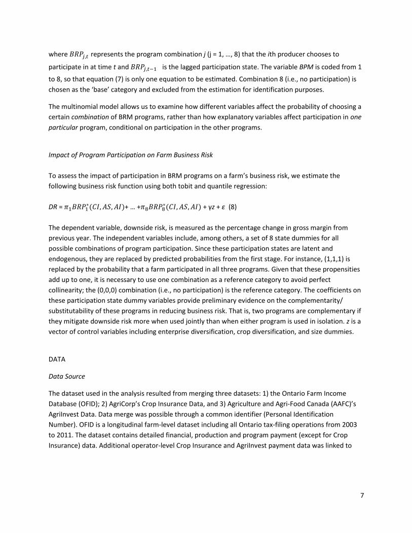
where represents the program combination j (j = 1, …, 8) that the ith producer chooses to
participate in at time t and is the lagged participation state. The variable BPM is coded from 1
to 8, so that equation (7) is only one equation to be estimated. Combination 8 (i.e., no participation) is
chosen as the ‘base’ category and excluded from the estimation for identification purposes.
The multinomial model allows us to examine how different variables affect the probability of choosing a
certain combination of BRM programs, rather than how explanatory variables affect participation in one
particular program, conditional on participation in the other programs.
Impact of Program Participation on Farm Business Risk
To assess the impact of participation in BRM programs on a farm’s business risk, we estimate the
following business risk function using both tobit and quantile regression:
DR = + … +
+ γz + ε (8)
The dependent variable, downside risk, is measured as the percentage change in gross margin from
previous year. The independent variables include, among others, a set of 8 state dummies for all
possible combinations of program participation. Since these participation states are latent and
endogenous, they are replaced by predicted probabilities from the first stage. For instance, (1,1,1) is
replaced by the probability that a farm participated in all three programs. Given that these propensities
add up to one, it is necessary to use one combination as a reference category to avoid perfect
collinearity; the (0,0,0) combination (i.e., no participation) is the reference category. The coefficients on
these participation state dummy variables provide preliminary evidence on the complementarity/
substitutability of these programs in reducing business risk. That is, two programs are complementary if
they mitigate downside risk more when used jointly than when either program is used in isolation. z is a
vector of control variables including enterprise diversification, crop diversification, and size dummies.
DATA
Data Source
The dataset used in the analysis resulted from merging three datasets: 1) the Ontario Farm Income
Database (OFID); 2) AgriCorp’s Crop Insurance Data, and 3) Agriculture and Agri-Food Canada (AAFC)’s
AgriInvest Data. Data merge was possible through a common identifier (Personal Identification
Number). OFID is a longitudinal farm-level dataset including all Ontario tax-filing operations from 2003
to 2011. The dataset contains detailed financial, production and program payment (except for Crop
Insurance) data. Additional operator-level Crop Insurance and AgriInvest payment data was linked to
8
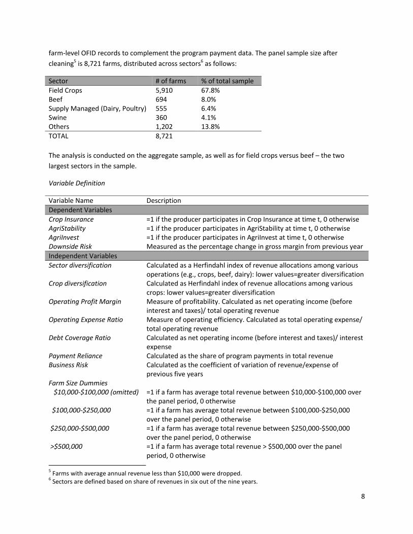
farm-level OFID records to complement the program payment data. The panel sample size after
cleaning5 is 8,721 farms, distributed across sectors6 as follows:
The analysis is conducted on the aggregate sample, as well as for field crops versus beef – the two
largest sectors in the sample.
Variable Definition
Variable Name Description
Dependent Variables
Crop Insurance =1 if the producer participates in Crop Insurance at time t, 0 otherwise AgriStability =1 if the producer participates in AgriStability at time t, 0 otherwise AgriInvest =1 if the producer participates in AgriInvest at time t, 0 otherwise Downside Risk Measured as the percentage change in gross margin from previous year
Independent Variables
Sector diversification Calculated as a Herfindahl index of revenue allocations among various operations (e.g., crops, beef, dairy): lower values=greater diversification
Crop diversification Calculated as Herfindahl index of revenue allocations among various crops: lower values=greater diversification
Operating Profit Margin Measure of profitability. Calculated as net operating income (before interest and taxes)/ total operating revenue
Operating Expense Ratio Measure of operating efficiency. Calculated as total operating expense/ total operating revenue
Debt Coverage Ratio Calculated as net operating income (before interest and taxes)/ interest expense
Payment Reliance Calculated as the share of program payments in total revenue Business Risk Calculated as the coefficient of variation of revenue/expense of
previous five years Farm Size Dummies $10,000-$100,000 (omitted) $100,000-$250,000 $250,000-$500,000 >$500,000
=1 if a farm has average total revenue between $10,000-$100,000 over the panel period, 0 otherwise =1 if a farm has average total revenue between $100,000-$250,000 over the panel period, 0 otherwise =1 if a farm has average total revenue between $250,000-$500,000 over the panel period, 0 otherwise =1 if a farm has average total revenue > $500,000 over the panel period, 0 otherwise
5 Farms with average annual revenue less than $10,000 were dropped.
6 Sectors are defined based on share of revenues in six out of the nine years.
9
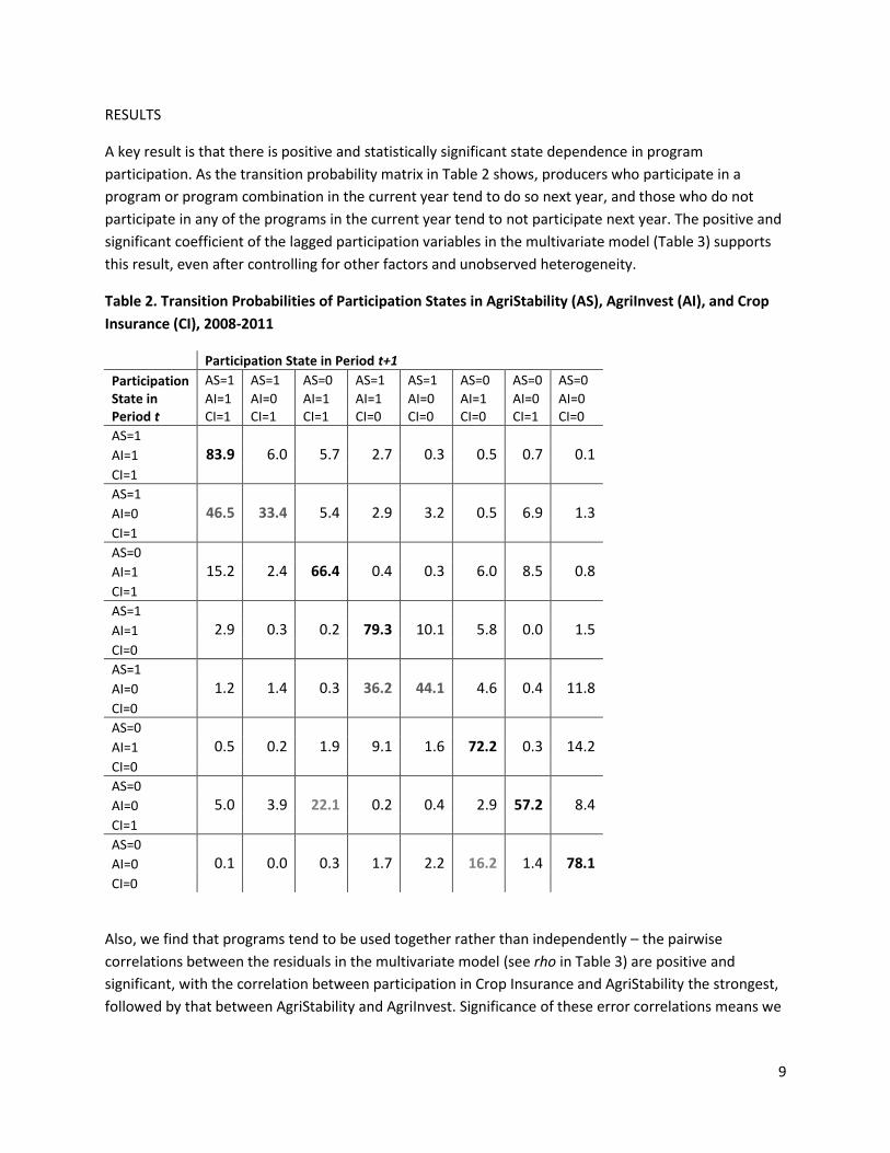
RESULTS
A key result is that there is positive and statistically significant state dependence in program
participation. As the transition probability matrix in Table 2 shows, producers who participate in a
program or program combination in the current year tend to do so next year, and those who do not
participate in any of the programs in the current year tend to not participate next year. The positive and
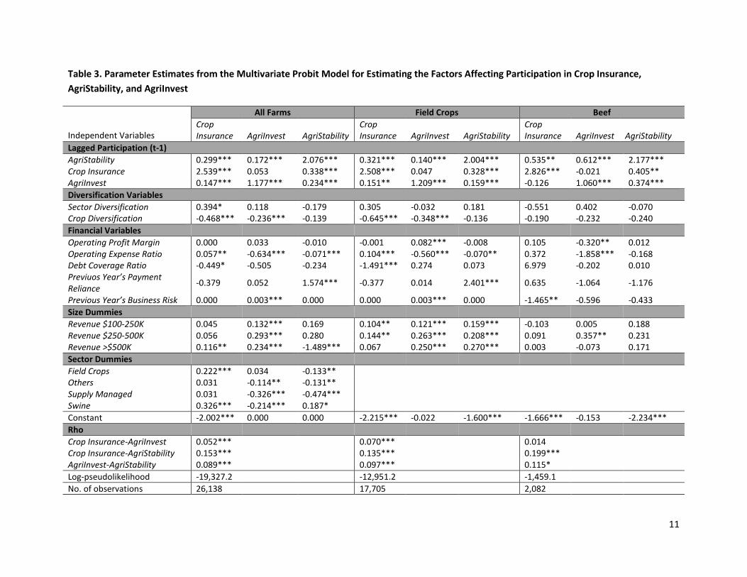
significant coefficient of the lagged participation variables in the multivariate model (Table 3) supports
this result, even after controlling for other factors and unobserved heterogeneity.
Table 2. Transition Probabilities of Participation States in AgriStability (AS), AgriInvest (AI), and Crop
Insurance (CI), 2008-2011
Also, we find that programs tend to be used together rather than independently – the pairwise
correlations between the residuals in the multivariate model (see rho in Table 3) are positive and
significant, with the correlation between participation in Crop Insurance and AgriStability the strongest,
followed by that between AgriStability and AgriInvest. Significance of these error correlations means we