Sufficient Statistics for Welfare Analysis:A Bridge Between Structural and Reduced-Form Methods

Raj Chetty UC-Berkeley and NBER

September 2008

MOTIVATION

• Two competing paradigms for policy evaluation and welfare analysis: “structural” vs. “reduced-form”

• Structural approach generally involves two steps: estimate primitives of a model and then simulate effects of policies on welfare

• Critique: difficult to identify full primitive structure without implausibly strong assumptions.

• Reduced-form: estimate statistical relationships using transparent, exogenous sources of variation for identification (“treatment effects”)

• Critique: Estimates not useful for welfare analysis because they are not deep parameters; endogenous to policy regime (Lucas 1976, Heckman and Vytlacil 2005)

SUFFICIENT STATISTICS

• Past decade of work in public economics provides a strategy that bridges the gap between the two methods

• Idea: Instead of primitives, identify “sufficient statistics” for welfare analysis that can be estimated using reduced-form methods

• Any set of primitives (

consistent with sufficient statistics (

generates the same value of welfare gain (dW/dt)

1t 2t

prefs.,

= f(,t) dW/dt used for constraints y = 1 X1 + 2 X2 +

policy analysis

dWdt t

not uniquely

identified usingidentified program evaluation

Structural Sufficient WelfarePrimitives Statistics Change

THE SUFFICIENT STATISTIC APPROACH

Intellectual History

• Idea that it is adequate to estimate “sufficient statistics” to answer some questions dates to Marschak (1954) and Koopmans (1954)

• But applied to a wide range of policy questions only in past decade

• 1950-70s – simple structural models fit to macro and micro data

• 1980s: concerns about identification of non-linear structural models with heterogeneity (e.g. Ashenfelter 1978, LaLonde 1985)

• Reduced-form, quasi-experimental methods (e.g. Angrist 1990, Card and Krueger 1995; Imbens and Wooldridge 2008)

• 1990s: Large body of “program evaluation” estimates developed

Most recent literature integrates program evaluation estimates with structural models to make statements about welfare

OBJECTIVES OF THIS TALK

1. Codify main steps and concepts of sufficient statistic approach

2. Review a set of applications, showing how several independent papers are variants on this theme

3. Discuss benefits and costs of this strategy vs. structural methods

Advantages: identify fewer parameters, weaker modelling assumptions

Disadvantages: only local welfare analysis, “black box” (no evaluation of model)

Sufficient statistic methods provide a useful complement to (rather than a substitute for) structural methods in future work

OUTLINE

1. Harberger (1964) and Extensions

2. General Framework

3. Application 1: Taxation

4. Application 2: Social Insurance

5. Application 3: Behavioral Models

6. Summary of Advantages/Disadvantages

HARBERGER (1964)

• Precursor to modern sufficient statistic literature: Harberger’s partial- equilibrium analysis of deadweight cost of taxation

• Simple model that is useful to build intuition about more sophisticated applications discussed later

• Objective: calculate excess burden (EB) of tax. How much extra revenue could be raised by lump sum taxation, keeping utility constant?

• To simplify exposition, ignore income effects (quasilinear utility)

Setup

• Individual endowed with Z units of good y (numeraire)

• Normalize price of y to 1

• Firms convert numeraire y into J other consumption goods (x1 ,…xJ )

• Producing xj units of good j requires cj (xj ) units of numeraire

• Let c(x) = cj (xj ) denote total cost of producing vector x

• Production perfectly competitive

• Let p = (p1 ,…,pJ ) denote prices of produced goods

• Government levies a unit tax t on good 1

• Goal: measure efficiency cost of this tax (social surplus from transactions that do not occur because of tax)

• Consumers take prices as given and solve

• Representative firm takes p as given and solve

• Two problems define demand supply fns. Equilibrium:

• Social welfare: sum of utility, profits, and tax revenue

maxx,y

ux1, . . . ,xJ y

s.t. px tx1 y Z

maxx px − cx

xDp xSp

Wt maxx ux Z − tx1 − px maxx px − cx tx1

maxx ux Z − tx1 − cx tx 1

Calculation of Excess Burden

• Structural method: Estimate J good supply + demand system and recover u(x) and c(x)

• Ex: use Stone-Geary or AIDS and CES production functions

• Or non parametric methods to recover preferences and technology as in Hausman (1981) and Hausman and Newey (1994)

• Econometric challenge: simultaneity.

• Need 2J instruments to identify supply and demand in J markets.

Harberger Approach

• Private sector choices are made to maximize term in curly brackets (private surplus) in social welfare function

• Envelope conditions for (x1 ,…,xJ ) yield simple formula:

• Tax induces changes in x and p, but these responses do not have a first-order effect on private surplus b/c of optimization

• Loss in surplus determined purely by difference between WTP and cost of good x1 (triangle between demand and supply)

dx1 /dt is a “sufficient statistic” for calculating dW/dt.

• Do not need to identify primitives, simplifying identification.

dWdt −x1 x1 t dx1

dt t dx1dt

Wt maxx ux Z − tx1 − cx tx1

Heterogeneity

• Benefit of sufficient statistic approach is particularly evident in a model that permits heterogeneity across individuals

• N agents with wealth Zi and utility functions

• Social welfare:

• Structural method requires estimation of demand systems for all agents

• Sufficient statistic formula is unchanged – still need only slope of aggregate demand dx1 /dt

ui xi y

Wt ∑i1N maxxi uixi Zi − tx1

i − cx t∑i1N x1

i

dWdt −∑i1

N x1i ∑ i1

N x1i t

d∑ i1N

x1i

dt t dx1dt

Discrete Choice

• Now suppose individuals can choose only one of the J products

• E.g. car models, modes of transportation, or neighborhoods

• Each product j characterized by a vector of K observable attributes

and an unobservable attribute j

• Agent i’s utility from choice j is

• Let Pij denote probability i chooses product j, Pj total expected demand for product j, and cj (Pj ) cost of production

xj x 1j,...,xKj

uij vij ij

with v ij Zi − pj j ixj

• Assume ij has a type 1 extreme value distribution (mixed logit)

• Then probability individual i chooses product j is

and consumer i’s expected surplus is

• Aggregating over consumers and including producer profits gives

Pij expvij

∑ jexpvij

Si p1, . . . ,pJ E maxui1, . . . ,uiJ log∑ j expv ij

W ∑ i log∑j expv ij pP − cP

• Structural approach to policy analysis: identify i and c(P) using methods e.g. in Berry (1994) or BLP (1995)

• Sufficient statistic: two examples

1. Tax on good 1. Then easy to establish that

2. Tax on all products in the market.

where Ep = total expenditure on products in the market

• Do not need to estimate substitution patterns within market

• Microeconomic demands not smooth but expected welfare is use similar envelope conditions

dWdt t dP1

dt

dWd ∑ j pj

dPj

d dEPd

GENERAL FRAMEWORK

• Modern sufficient statistic approach builds on Harberger’s idea

• First present a general framework that nests papers in this literature

• Explains why identification of a few sufficient statistics is adequate to answer many questions

• Provides a “recipe” for deriving such formulas in future work

• Abstractly, many government (price intervention) policies amount to levying a tax t and paying a transfer T(t)

• Redistributive taxation: transfer to another agent

• Social insurance: transfer between states

• Excess burden: transfer used to finance lump sum grant

• Develop a rubric to calculate dW/dt using sufficient statistics

Step 1: Specification of General Structure of Model

• Government levies tax on x1 and pays transfer T(t) in units of xN

• Utility: U(x1 ,…,xN )

• Constraints: G1 (x,t,T),….,GM (x,t,T)

• Private sector takes t and T as given and solves

• Note that this nests case of competitive production, with U(x)=u(x)-c(x) because decentralized eq. maxes total surplus

maxUx1, . . . ,xJ

s.t. G1x, t, T 0, . . . ,GMx, t,T 0

Step 2: Multiplier Representation for dW/dt

• Social welfare:

• Using envelope thm., welfare gain from increasing t is:

• Key unknowns: multipliers m

• Other parameters known mechanically from constraints

dWdt ∑m1

M m∂Gm∂T

dTdt

∂Gm∂t

Wt maxx1,...,xJ Ux1, . . . , xJ ∑m1M mGmx, t,T

Step 3: Map Multipliers to Marginal Utilities

• Multipliers can typically be recovered by exploiting first-order conditions

• Private sector optimization requires

• Under a mild technical condition on structure of constraints, we obtain

where Kt , kT are known functions of equilibrium quantities

Problem reduced to recovery of only two marginal utilities rather than full structure (U, G)

u′ xi −∑m1M m

∂Gm∂xi

dWdt kT

dTdt u ′xN − ktu′x1

Step 4: Recover Marginal Utilities from Observed Choices

• Final step in deriving formula is to back out the two marginal utilities from empirically observable choices

• No canned procedure; applications illustrate various methods

• Usual trick: marginal utilities appear in first-order-conditions for choices back out from high-level elasticities of behavior

• Can generally express formulas in terms of parameters that can be estimated using program-evaluation methods

• Harberger example: u’(xN ) = 1 given quasilinearity. To recover u’(x1 ), use first order condition

u′ x1 p1 t

Step 5: Empirical Implementation

• Problem in empirical implementation: program evaluation studies estimate x1 /t not dx1 /dt where t = t1 - t0

• This can give information about change in welfare from t0 to t1

• Three options:

1. Bound W(t1 )-W(t0 )

2. Take a linear approximation to demands to calculate W(t1 )-W(t0 )

3. Estimate x(t,Z) non-parametrically if data and variation permit

• Analogous to estimating full distribution of MTEs (Heckman and Vytlacil 2005)

dWdt t ft, dx1

dt , dx1dZ , dx2

dt , dx2dZ , . . .

Step 6: Structural Evaluation

• Find a vector of that matches sufficient statistics, assess plausibility

• Run three types of simulations:

1. Compare exact simulated welfare gain with that implied by sufficient statistic formula given approximations made in step 5

2. Simulate how sufficient statistics vary with t; if highly non-linear, take into account in empirics

3. Use structural model to guide out-of-sample extrapolations and solve for globally optimal policy.

• This step is often not implemented, but is critical to make reliable out- of-sample predictions using sufficient statistic methods

• Problems with sufficient statistic approach evident when structural primitives are not assessed.

APPLICATION 1: TAXATION

Feldstein, Martin. “The Effect of Marginal Tax Rates on Taxable Income: A Panel Study of the 1986 Tax Reform Act,” Journal of Political Economy, 1995.

Diamond, Peter. “Optimal Income Taxation: An Example with a U-Shaped Pattern of Optimal Marginal Tax Rates," American Economic Review, 1998.

Saez, Emmanuel. “Using Elasticities to Derive Optimal Income Tax Rates,”Review of Economic Studies, 2001.

Other Sufficient Statistic References:

Piketty (Revue Francaise 1997)Gruber and Saez (JPubE 2002)Goulder and Williams (JPE 2003)Chetty (AEJ-EP forthcoming)

Feldstein (1995, 1999)

• Following Harberger, large literature in labor estimated effect of taxes on hours worked to assess efficiency costs of taxation

• Feldstein observed that labor supply involves multiple dimensions, not just choice of hours: training, effort, occupation

• Taxes also induce inefficient avoidance/evasion behavior

• Structural approach: account for each of the potential responses to taxation separately and then aggregate

• Feldstein’s solution: elasticity of taxable income with respect to taxes is a sufficient statistic for calculating deadweight loss

Setup

• Government levies linear tax t on reported taxable income

• Agent makes N labor supply choices: l1 ,…,lN

• Each choice li has disutility i (li ) and wage wi

• Agents can shelter $e of income from taxation by paying cost g(e)

• Taxable Income (TI) is

• Consumption is given by taxed income plus untaxed income

x N 1 − tTI e

TI ∑i1N wili − e

• Social welfare:

• Totally differentiating W(t) gives

• Use first order conditions to measure marginal utilities:

• Substituting into dW/dt yields Feldstein’s formula:

• Intuition: marginal social cost of reducing earnings through each margin is equated at optimum irrelevant what causes change in TI.

g′e ti′xi 1 − twi

dWdt dTI

dt dedt 1 − g′e − ∑i1

N i′l i

dl idt

Wt 1 − tTI e − ge − ∑i1N il i t TI

dWdt

t dTIdt

• Simplicity of identification in Feldstein’s formula has led to a large literature estimating elasticity of taxable income

• Problem: since primitives are not estimated, assumptions never tested

• Chetty (2008) questions validity of assumption that g’(e) = t

• Costs of many avoidance/evasion behaviors are transfers to other agents in the economy, not real resource costs

• In a model that permits such transfer costs, Feldstein’s formula is invalid because of externality associated with sheltering

• Instead, EB depends on weighted average of taxable income and total earned income elasticities

• Practical importance: even though reported taxable income is highly sensitive to tax rates for rich, efficiency cost may not be large!

• A structural approach would not have run into this problem because g(e) would have been identified.

Saez (2001)

• Saez characterizes optimal tax rates in Mirrlees’ (1971) model using high-level sufficient statistics

• Multiple policy instruments, continuum of heterogeneous agents

• Levy tax T(z) at income level z net-of-tax income: z-T(z)

• Mirrlees characterized optimal tax rates in terms of primitives that entered complex first-order-conditions

• Offers little intuition about key determinants of T(z)

• Simulations reach variable conclusions depending on primitives

Mirrlees Model

• Individuals choose labor supply to maximize

• Government chooses tax schedule T(z) to maximize social welfare

subject to resource and IC constraints

WTz 0

Gucw,T, wlw,TdFw

G1c,z, T 0

zw,TdFw − 0

cw, TdFw − E 0

G2c,z, T 1 − T′zw − ′lw 0

uc, l c − ls.t. c wl − Twl

• Diamond and Saez obtain following formula for optimal tax T(z):

• Elasticities (z), density h(z), and marginal utility g(z) at each point of income distribution together determine optimal tax rate

• Marginal social welfare weights taken as exogenous to system

• Not an explicit formula for optimal tax; can only be used as a test.

• To compute optimal tax system, Saez calibrates structural primitives to match three parameters that enter formula and then simulates T(z)

• Optimal income tax schedule is inverse-U-shaped, with a large lump sum grant and marginal rates ranging from 50-80%.

• Illustrates power of combining sufficient statistic and structural approaches to do more than marginal welfare analysis

Tz1−Tz 1

zzhz z

1 − gz ′hz ′dz ′

APPLICATION 2: SOCIAL INSURANCE

Gruber, Jonathan. “The Consumption Smoothing Benefits of Unemployment Insurance,” American Economic Review, 1997.

Chetty, Raj. “Moral Hazard vs. Liquidity and Optimal Unemployment Insurance,” Journal of Political Economy, 2008.

Shimer, Robert and Ivan Werning. “Reservation Wages and Unemployment Insurance,” Quarterly Journal of Economics, 2007.

Other Sufficient Statistic References:

Chetty (JPubE 2006)Einav, Finkelstein, and Cullen (2008)Finkelstein, Luttmer, and Notowidigdo (2008)Chetty and Saez (2008)

Static Model of Social Insurance (Baily 1978)

• Two states: high and low (unemployed, sick ,etc.).

• Income in high state: A + wh ; in low state: A + wl

• Consumption in high state: ch ; in low state: cl

• Agent can control probability of high state via effort e at cost (e)

• Reflects search effort, investment in health, etc.

• Choose units so that probability of high state is p(e)=e.

• Imperfect private insurance: individuals can transfer $z from high state to low state via informal risksharing at cost q(bp )

• $1 increase in cl $(1-e)/e+q(bp ) reduction in ch

• Social insurance: government pays a benefit b in low state financed by a tax t(b)=b(1-e)/e

• Social welfare:

• Marginal welfare gain has marginal-utility representation:

• To convert to money-metric, compare welfare gain of increasing insurance program and wage bill in high state:

MWb dWdbb/1−e

dWdwh

b/e u ′cl−u ′ch

u ′ch− 1−e,b

e

Wb euA wh − 1 − ee bp − qbp − tb

1 − euA wl bp b − e

dWdb 1 − eu′c l − 1

1−e,be u′ch

Sufficient Statistics

Recent literature on social insurance makes two contributions:

1. Shows that formula holds in a general class of dynamic models: arbitrary choices and constraints, stochastic wages, heterogeneity

• Distills analysis to two parameters; structural models often forced to assume no borrowing or private insurance

2. Recovers marginal utility gap from choice data:

• Gruber (1997): consumption

• Shimer and Werning (2007): reservation wages

• Chetty (2008): liquidity and substitution effects in effort

u ′ c l−u ′ c h

u ′c h fobservables

Gruber (1997)

• Quadratic approximation to utility function yields

• Gruber estimates a linear consumption function:

• Plugging back into Baily’s formula yields

• Gruber estimates

=0.24, = -0.28 using consumption data from PSID and state-level changes in UI benefits in the U.S.

• With

= 1, obtains dW/db < 0; extrapolating to lower benefit levels, concludes that optimal benefit near 0.

• Limitation: value of

is highly debated; may vary with context.

Δcc hb b

dWdb b − 1−e,b

e

u ′ c l−u ′ c h

u ′c h Δc

c hb

Chetty (2008)

• Uses comparative statics of effort choice (e) to back out marginal utils.

• First order condition for effort:

• Effects of cash grant (e.g. severance pay) and higher benefit level:

• It follows that

• Liquidity effect (de/dA) measures completeness of private insurance; moral hazard effect (de/dwh ) measures efficiency cost of insurance.

′ e uc h − ucl

u′cl − u ′chu′ch

−∂e/∂A∂e/∂A − ∂e/∂b

MWb −∂e/∂A∂e/∂A − ∂e/∂b −

1−e,be

∂e/∂A u′ch − u′cl/′′e ≤ 0∂e/∂b −u′cl/′′e

145

150

155

160

165

Mea

n N

onem

ploy

men

tDur

atio

n (d

ays)

12 18 24 30 36 42 48 54 60

Previous Job Tenure (Months)

Effect of Severance Pay on Nonemployment Durations in Austria

Card, Chetty and Weber (QJE 2007)

Calibration of Chetty (2008) formula

• Chetty estimates de/dA0 and de/db using quasi-experimental variation in UI laws and severance payments.

• Plugging estimates into formula for dW/db, Chetty calculates dW/db

• Welfare gain from raising weekly benefit level by 10% from current level in U.S. (50% wage replacement) is $5.9 bil = 0.05% of GDP

• Uses structural model calibrated to match sufficient statistics to assess policy implications

• dW/db falls rapidly with b, suggesting we are near optimum

• Also conducts simulations of other policies, e.g. provision of liquidity through loans.

Combine structural and sufficient stat. approaches to extent beyond marginal policy analysis in a credible manner.

Figure 1Marginal Welfare Gain vs. Initial Benefit Level

Benefit level (b)

Mar

gina

l Wel

fare

Gai

n fro

m R

aisi

ng B

enef

it Le

vel (

)

Chetty (2008) approximate formula

Exact

dW db

APPLICATION 3: BEHAVIORAL MODELS

Chetty, Raj, Adam Looney, and Kory Kroft. “Salience and Taxation: Theory and Evidence.” American Economic Review, forthcoming.

Bernheim, Douglas and Antonio Rangel. “Beyond Revealed Preference: Choice-Theoretic Foundations for Behavioral Welfare Economics,” Quarterly Journal of Economics, forthcoming.

Orig.Tag

Exp.Tag

-.1-.0

50

.05

.1

-.02 -.015 -.01 -.005 0 .005 .01 .015 .02

Figure 2aPer Capita Beer Consumption and State Beer Excise Taxes

Cha

nge

in L

og P

er C

apita

Bee

r Con

sum

ptio

n

Change in Log(1+Beer Excise Rate)

-.1-.0

50

.05

.1

-.02 -.015 -.01 -.005 0 .005 .01 .015 .02

Figure 2bPer Capita Beer Consumption and State Sales Taxes

Cha

nge

in L

og P

er C

apita

Bee

r Con

sum

ptio

n

Change in Log(1+Sales Tax Rate)

Chetty, Looney, Kroft (2008): Welfare Analysis in Behavioral Models

• Existing results on optimal tax/transfer policy are based on models inconsistent with preceding evidence.

• Need an alternative method of analyzing welfare consequences (incidence, efficiency costs) in view of evidence to make progress.

Objective: Develop formulas for incidence and efficiency costs of taxes that allow for salience effects

• Many potential positive models for salience effects (cognitive costs, heuristics, psychological factors); difficult to distinguish

• Therefore develop a method of welfare analysis that does not rely on a specific positive model of optimization errors

Setup

• Two goods, x1 and x2 ; normalize price of x2 to 1

• Good x2 untaxed. Government levies a tax t on x1 ; tax not included in the posted price (not salient).

• Representative consumer has quasilinear utility:

• Key deviation from standard neoclassical model: do not assume that x1 is chosen to maximize U(x1 )

• Instead, take demand x1 (p,t) as an empirically estimated object, permitting dx1 /dp ≠dx1 /dt

• Place no structure on demand functions except for feasibility:

Ux1 ux 1 Z − p tx1

p tx 1p, t x 2p, t,Z Z

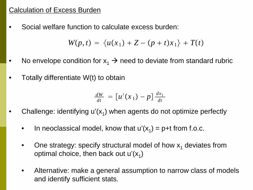
Calculation of Excess Burden

• Social welfare function to calculate excess burden:

• No envelope condition for x1 need to deviate from standard rubric

• Totally differentiate W(t) to obtain

• Challenge: identifying u’(x1 ) when agents do not optimize perfectly

• In neoclassical model, know that u’(x1 ) = p+t from f.o.c.

• One strategy: specify structural model of how x1 deviates from optimal choice, then back out u’(x1 )

• Alternative: make a general assumption to narrow class of models and identify sufficient stats.

dWdt u ′x 1 − p dx1

dt

Wp, t ux1 Z − p tx1 Tt

Preference Recovery Assumption

A1 When tax inclusive prices are fully salient, the agent chooses the same allocation as a fully optimizing agent:

Two steps in efficiency calculation:

1. Use price-demand x(p,0) to recover utility as in standard model

2. Use tax-demand x(p,t) to calculate W(t) and EB

• Easy to illustrate graphically in case of quasilinear utility

x1p, 0 x1∗p, 0 arg maxux1p, 0 Z − pxp, 0

Figure 4Excess Burden with Quasilinear Utility and Fixed Producer Prices

x

0p

0x

)(')0,( xupx

AB

C

D EG

H

F

1x*1x

I

EB ≃ − 12 t2 ∂x/∂t

∂x/∂p ∂x/∂t

p,t

xp 0, t

p 0 t

t ∂x/∂ t∂x/∂p

t ∂x∂t

Formula for EB with Optimization Errors

• When utility is quasilinear, excess burden of a small tax t is

where

• Simple modification of Harberger formula: price (or wage) and tax elasticities are together sufficient statistics

• Similar simple modification of standard formula for tax incidence

• Formula permits arbitrary optimization errors w.r.t. taxes, but requires optimization w.r.t. prices

EB ≃ − 12 t2 ∂x∂t ∂x

∂t / ∂x∂p

SUFFICIENT STATISTIC VS. STRUCTURAL APPROACHES

Advantages:

1. Simplifies identification: permits focus on estimating dx1 /dt using transparent, design-based methods (e.g. experiments)

• Can therefore be implemented with fewer assumptions than structural method (e.g. arbitrary heterogeneity)

2. Can be applied when positive model unclear

Disadvantages:

1. Can only be used for local welfare analysis around observed policies unless paired with structural model

2. “Black box”: welfare analysis never “theory free.”

• Primitives not identified cannot determine if assumptions consistent with data (Feldstein 1995, Gruber 1997)

Combining Structural and Sufficient Statistic Methods

• Sufficient statistic formulas should be used in combination with structural methods

• Evaluate structural model by testing whether its prediction for marginal welfare gains match sufficient statistic prediction

• Use structural model for overidentification tests of validity of general model used to derive suff stat. formula

• Calibrate structural model to match key moments for welfare

• Make out-of-sample predictions (e.g. optimal policy) guided by structural model

Can pick a point on interior of continuum between program evaluation and fully structural work.

POTENTIAL APPLICATIONS

• [ Labor] Training programs, minimum wage

• Lee and Saez (2008) – optimal minimum wage is a function of employment elasticity w.r.t. minimum wage

• [ Macro] Intertemporal behavior, growth models

• Aguiar and Hurst (JPE 2005) vs Scholz et al. (JPE 2006): identify key moments for calibrations.

• [IO] Analysis of competition policy, regulation

• Challenge: allowing for strategic interactions and non-marginal changes