HAL Id: tel-02060436 https://tel.archives-ouvertes.fr/tel-02060436 Submitted on 7 Mar 2019 HAL is a multi-disciplinary open access archive for the deposit and dissemination of sci- entific research documents, whether they are pub- lished or not. The documents may come from teaching and research institutions in France or abroad, or from public or private research centers. L’archive ouverte pluridisciplinaire HAL, est destinée au dépôt et à la diffusion de documents scientifiques de niveau recherche, publiés ou non, émanant des établissements d’enseignement et de recherche français ou étrangers, des laboratoires publics ou privés. Recommendation systems for online advertising Sumit Sidana To cite this version: Sumit Sidana. Recommendation systems for online advertising. Computers and Society [cs.CY]. Université Grenoble Alpes, 2018. English. NNT : 2018GREAM061. tel-02060436
Transcript
HAL Id: tel-02060436https://tel.archives-ouvertes.fr/tel-02060436
Submitted on 7 Mar 2019
HAL is a multi-disciplinary open accessarchive for the deposit and dissemination of sci-entific research documents, whether they are pub-lished or not. The documents may come fromteaching and research institutions in France orabroad, or from public or private research centers.
L’archive ouverte pluridisciplinaire HAL, estdestinée au dépôt et à la diffusion de documentsscientifiques de niveau recherche, publiés ou non,émanant des établissements d’enseignement et derecherche français ou étrangers, des laboratoirespublics ou privés.
Recommendation systems for online advertisingSumit Sidana
To cite this version:Sumit Sidana. Recommendation systems for online advertising. Computers and Society [cs.CY].Université Grenoble Alpes, 2018. English. NNT : 2018GREAM061. tel-02060436
DOCTEUR DE LA COMMUNAUTÉ UNIVERSITÉ GRENOBLE ALPESSpécialité : Mathématiques et InformatiqueArrêté ministériel : 25 mai 2016
Présentée par
Sumit SIDANA
Thèse dirigée par Massih-Reza AMINI, Professeur, Université Grenoble Alpes
préparée au sein du Laboratoire Laboratoire d'Informatique de Grenobledans l'École Doctorale Mathématiques, Sciences et technologies de l'information, Informatique
Filtrage collaboratif en ligne : application à lapublicité programmatique
Dynamic collaborative filtering for on-line advertising
Thèse soutenue publiquement le 8 novembre 2018,devant le jury composé de :
Monsieur MASSIH-REZA AMINIPROFESSEUR, UNIVERSITE GRENOBLE ALPES, Directeur de thèse Madame CHARLOTTE LACLAUMAITRE DE CONFERENCES, UNIVERSITE JEAN MONNET - SAINT-ETIENNE, Co-directeur de thèseMonsieur PATRICK GALLINARIPROFESSEUR, SORBONNE UNIVERSITES - PARIS, Rapporteur Madame JOSIANE MOTHEPROFESSEUR, UNIVERSITE TOULOUSE-JEAN JAURES, Rapporteur Madame SIHEM AMER-YAHIADIRECTRICE DE RECHERCHE, CNRS DELEGATION ALPES, Président Monsieur ROMARIC GAUDELPROFESSEUR ASSISTANT, ENSAI - RENNES, Examinateur Monsieur GILLES VANDELLERESPONSABLE SCIENTIFIQUE, SOCIETE KELKOO - ECHIROLLES, Examinateur
AcknowledgmentsFirst of all, I would like to express my gratitude to my supervisor Massih-Reza Aminiand co-supervisor Charlotte Laclau. I am grateful for your guidance, patience, advice,time-involved, and for the research ideas shared with me during these three years.The encouragement, guidance and resources you provided helped me to continue myresearch and finish this thesis.
Then, I would like to thank Patrick Gallinari and Josiane Mothe, who kindly agreedto review my Ph.D. thesis. I would also like to thank Gilles Vandelle and RomaricGaudel, who agreed to be part of my thesis committee.
Thanks to Sihem Amer-Yahia of CNRS, who first gave me an opportunity of in-ternship in LIG, where I got my first research experience, and which encouraged me tostart a PhD. I am also grateful to you for agreeing to be part of my thesis committee.
Thank you to my parents for their emotional support and encouragement duringthis PhD.
Thanks to all the AMA members (past and present) for their help and support:Bikash, Sami, Parantapa, Hamid, Yagmur, Vera, Karim, Thibaut, Anil, Julien, Myriam,Georgios, Adrien, Maziar, Hesam, Lauren, Saeed, Saeid and Vasilii.
Thanks to LIG and Universite Grenoble Alpes for their financial and logisticalsupport. Thanks to FUI for their financial participation in this thesis.
Thanks to Kelkoo and Purch engineers for providing data and advice in this PhD.
ii
Abstract
This thesis is dedicated to the study of Recommendation Systems for im-plicit feedback (clicks) mostly using Learning-to-rank and neural networkbased approaches. In this line, we derive a novel Neural-Network modelthat jointly learns a new representation of users and items in an embeddedspace as well as the preference relation of users over the pairs of itemsand give theoretical analysis. In addition we contribute to the creation oftwo novel, publicly available, collections for recommendations that recordthe behavior of customers of European Leaders in eCommerce advertis-ing, Kelkoo1 and Purch2. Both datasets gather implicit feedback, in formof clicks, of users, along with a rich set of contextual features regardingboth customers and offers. Purch’s dataset, is affected by popularity bias.Therefore, we propose a simple yet effective strategy on how to overcomethe popularity bias introduced while designing an efficient and scalablerecommendation algorithm by introducing diversity based on an appro-priate representation of items. Further, this collection contains contextualinformation about offers in form of text. We make use of this textual in-formation in novel time-aware topic models and show the use of topicsas contextual information in Factorization Machines that improves perfor-mance. In this vein and in conjunction with a detailed description of thedatasets, we show the performance of six state-of-the-art recommendermodels.
Keywords. Recommendation Systems, Data Sets, Learning-to-Rank, Neu-ral Network, Popularity Bias, Diverse Recommendations, Contextual in-formation, Topic Model.
U ⊆ N ; U = u1, · · · , un is the set of n users or the set of indexes over usersI ⊆ N ; I = i1, · · · , im is the set of m items or the set of indexes over itemsR = a sparse preference matrix of size n×mrui = Rating given by user u for item i
rui = Predicted rating of target user u of item i
pu = Latent feature vector of user uqi = Latent feature vector of item i
(i, u, i′) = A triplet composed by the indexes of an item i, a user u and a second item i′
u = Preference relation
Uu = The transformed embedding vector of user uVi = The transformed embedding vector of item i
Sn = A random set of size n of interactions by building triplets (i, u, i′)
Nu,k = A ranked list of the k M preferred items for each user in the test setSku = the list of items and k its sizeV`1i (resp. V`1
i′ ) = the `1-normalized embedding associated with item i (resp. i′)β is the diversity inducing regularization parameter whose role is to induce more orless diversity in the final list of recommended itemsP = PostsG = RegionsT = Time periodsPtg = Posts from region g during time tDtg = Document-set built by mapping the content of each post p ∈ Ptg to a document
1
CONTENTS CONTENTS
2
1. INTRODUCTION
Chapter 1
Introduction
In the recent years, recommender systems (RS) have attracted a lot of interest in bothindustry and academic research communities, mainly due to new challenges that thedesign of a decisive and efficient RS presents. Given a set of customers (or users), thegoal of RS is to provide a personalized recommendation of products to users whichwould likely to be of their interest. This process is described in Figure 1.1. Commonexamples of applications include the recommendation of movies (Netflix, AmazonPrime Video), music (Pandora), videos (YouTube), news content (Outbrain) or ad-vertisements (Google). The development of an efficient RS is critical from both thecompany and the consumer perspective. On one hand, users usually face a very largenumber of options: for instance, Amazon proposes over 20,000 movies in its selec-tion, and it is therefore important to help them to take the best possible decision bynarrowing down the choices they have to make. On the other hand, major companiesreport significant increase of their traffic and sales coming from personalized recom-mendations: Amazon declares that 35% of its sales is generated by recommendations,two-thirds of the movies watched on Netflix are recommended and 28% of ChoiceS-tream users said that they would buy more music, provided the fact that they meet theirtastes and interests.1
This thesis is part of the FUI project Calypso, which is designed with the maingoal of improving the performance of the e-commerce advertisements, that will begenerating a large part of the income of the partner companies, namely Kelkoo and
1Talk of Xavier Amatriain - Recommender Systems - Machine Learning Summer School 2014 @CMU.
3
1. INTRODUCTION
Figure 1.1 – A model is learned based on the set of available user preferences overitems. It is then used to recommend new items to the same set of users (or new users).
Purch. With the help of predictive machine learning approaches, the project proposesto increase the probability of clicking on the products presented to Internet users inadvertising inserts on the sites of both partners and purchased on advertising marketplaces. Internet advertising has become a major economic challenge for online sellingcompanies that have to optimize their catalogs in real time, in order to propose theproducts to users that fit the best to their interests and preferences. The companies arerequired to display advertisements and offers which user may be interested in engagingand buying. The overall model needs to address several challenges including but notlimited to, being scalable in order to deal with a large amount of data, work withhighly sparse and implicit feedback, and being able to handle heterogeneous contextualinformation regarding both the users and the products.
1.1 Challenges in Online Adverstising
While building efficient and scalable models for online advertising, there are variouschallenges and issues which need to be addressed. These are as follows.
Types of feedback
The majority of approaches for RS are based on the previous feedback given by theusers of the system. These feedback can be of different nature when items are presentedto her/him, and we broadly classify them as being either implicit or explicit.
Explicit feedback is probably the most common one in the literature, and can be in
4
1. INTRODUCTION
the form of ratings1, up-votes or likes, for instance. However, while explicit feedbackgenerally provides a relevant signal for making recommendation, it is also much moredifficult to gather than implicit one, as one needs to convince the user to rate or ex-plicitly tell their preference after having consumed the item. For this reason, feedbackused for building efficient RS has evolved over time, from explicit feedback to mostlyimplicit one.
Implicit feedback is usually inferred from user’s behavior while interacting withthe system, and include clicking on items, bookmarking a page or listening to a song.Implicit feedback, as contrary to explicit feedback, is in abundance and does not re-quire an extra effort from user’s side. However, it also presents several challengingcharacteristics. Firstly, implicit feedback does not clearly depict the preference of auser for an item; for instance a user listening to a song or clicking on a product doesnot necessarily mean that he or she likes the corresponding item. For this reason, onecannot measure the degree of preference from such type of interactions. Secondly,these data present a scarcity of negative feedback, i.e., only positive observations. Thisis because a user not clicking on a product may be because of various reasons, suchas, lack of time, or the offer not being in display region of the banner. For this rea-son, considering the lack of any positive signal as a negative signal introduces bias inbuilding models. There are no true negatives in implicit feedback.
However, because of its presence in abundance and availability, research on im-plicit feedback has gained increasing attention in very recent years [He et al., 2016]and have been greatly encouraged by competitions organized by some of the majorindustrial actors, like Criteo2, Outbrain3, or Spotify4, for instance.
Sparsity
Given large sets of users and items, sparsity arises from the fact that users in generalrate or click only a very limited number of items, compared to the number of itemsavailable in the catalogue that are shown to them. This problem is extremely commonin recommender systems, see for example the degree of sparsity present in RS bench-
marks shown in Table 1.1, and needs to be taken into account while designing a RS.In addition, for data extracted from online advertising, which interests us in this thesis,this phenomenon is even more pronounced.
Table 1.1 – Statistics of various collections used in our experiments after preprocessing.# of users # of items # of interactions Sparsity
Finally, popularity-bias is another prevalent issue in RS and raises the question of howwe recommend instead of just what we recommend to the users.
Indeed, the goal of a RS is to have fewer flops on the top [Paudel et al., 2017] ofthe recommended list, and inducing more diversity in this recommended list ensuresthat user may prefer to interact with at least some items in contrast to the situationwhere we introduce just monotonous relevant items. In addition, the recent work of[Abdollahpouri et al., 2017] shows that diversity can be used in order to control thepopularity bias in such type of data, also known as the problem of long tail i.e. asituation where a large majority of items have only very few ratings or clicks, eitherbecause they are new or just unpopular. In recent works [Herlocker et al., 2004; McNeeet al., 2006], it has been shown that only recommending relevant items (within thesemantics of items which are the more likely to be of interest for users) has its limitsand that adding notions of diversity and discovery in the process can highly increasethe performance of a recommendation system [Bradley and Smyth, 2001; McSherry,2002; Smyth and McClave, 2001; Zhang and Hurley, 2008].
1.2 Contributions
In this thesis, we tried to address these challenges by exploring different type of RSmodels.
6
1. INTRODUCTION
These models are mainly evaluated on the basis of two newly created datasets,KASANDR and PANDOR, arising from the real online traffic recorded by the two part-ners of the project, and that we made publicly available to the research community,along with a detailed description. We show that PANDOR, in particular, suffers frompopularity bias and propose diversity based approach, which are based on regulariza-tion, in order to handle diversity.
Then, in order to deal with the textual content in that we had in hand, we developtwo novel time-aware topic modelling approaches, which are able to extract latenttopics in temporally sequenced textual data. We show that topics derived from thistime-aware topic model can be used to improve the performance of RS models.
Furthermore, for the personalized recommendation part, we propose a novel neural-network based architecture which can handle data sparsity by learning both a gooddense representation of users and items, as well as the ranked list of the preferencesfor all users. This model, in addition to be efficient with implicit feedback, also allowsto deal with large datasets and can easily integrate contextual information, of diversenature.
1.3 Thesis structure
The rest of this thesis is organized into 5 chapters. The main contents of each chapterare summarized below:
Chapter 2 : Describes some common state-of-the-art approaches developed in RS.We mainly focused on collaborative filtering, learning to rank, item-embedding anddiversity based approaches for recommender systems as our contributions also buildupon these ideas.
Chapter 3 : Presents in detail large scale data sets we have contributed to RS com-munity during the discourse of this thesis. In particular, we describe basic character-istics of KASANDR and PANDOR and how making them public can help RS researchcommunity to benchmark their approaches and models on these data sets.
7
1. INTRODUCTION
Chapter 4 : Details the topic-modelling techniques to extract evolution of latent con-cepts with time from textual data and how they can be applied in context of RS. We firststudy general purpose topic modeling techniques. Then, we present two novel time-aware topic models. We study these approaches as an application to health monitoringand run experiments to show how our models outperform the existing techniques topredict the evolution of topics with time.
Chapter 5 : Presents a neural network to optimize two loss functions simultaneouslyin order to come up with better representation and ranking functions. In particular, welearn embedding based representations and pairwise ranking function by optimizingtwo losses simultaneously. We then extend this neural network to recommend, notonly relevant offers, but diverse offers as well.
Chapter 6 : Sets out the experiments we conducted in order to show the efficiencyof our models. We first study various settings of the parameters and their effects onperformance of the neural network we developed. Then, we go on to show that it out-performs the existing techniques in recommending offers when the prediction functionis learned using implicit feedback. Then, we give benchmark results on popular RS al-gorithms which have been known to perform well on implicit feedback on KASANDR.Then, we run experiments on PANDOR and present results of various baselines. Weshow that baselines run on PANDOR suffer from popularity bias and performance ofmodels can be improved by using diversity based regularizers. We also show the resultsof the models can be improved by using topics from time-aware topic models.
8
2. RECOMMENDER SYSTEMS: STATE-OF-THE-ART AND EVALUATION
Chapter 2
Recommender Systems:state-of-the-art and evaluation
9
2. RECOMMENDER SYSTEMS: STATE-OF-THE-ART AND EVALUATION
2.1 Definition of Personalized Recommendation
Personalized recommendations consist of selecting products or offers from the catalogthat create a relevant, individualized interaction environment designed to enhance theexperience of the user. It uses insight based on the user’s personal data, as well asbehavioral data about the actions of similar individuals, to deliver an experience thatmeets specific needs and preferences. Advantage of using personalized approachesto recommendation is that these approaches generally outperform non-personalizedcounterparts in performance and are interesting both from academic and industry pointof view.
Before the breakthrough of ML in RS, recommendations were made based on non-ML approaches, such as for instance, random-based approach, consisting of recom-mending random items to a given user, or popularity-based approaches consisting ofrecommending the most popular items to all users. While these type of approaches areusually outperformed by personalized recommendation methods, they can still be usedto deal with specific challenges such as user and item cold-start.
In this chapter, we give a brief overview of three families of RS models that arearguably the most widely used for our task, notably: collaborative filtering, learning-to-rank and deep learning. The remainder of this chapter is organized as follows.Section 2.2 describes the content filtering approaches principle, their advantages andproblems. Section 2.3 presents the general idea behind collaborative filtering (CF).We first define CF and then categorize them into memory-based CF and latent factormodels. Specifically, we describe Matrix Factorization, Factorization Machines. Then,in section 2.4, we discuss ranking-based CF approaches in detail. We discuss howpairwise learning-to-rank has been applied to recommender systems. In Section 2.5,we give details of how deep learning approaches have been successfully applied toRS. We discuss the concept of representation learning in detail. Finally, in section 2.7,we discuss various evaluation approaches widely used in RS and specifically the oneswhich are relevant to our contributions.
10
2. RECOMMENDER SYSTEMS: STATE-OF-THE-ART AND EVALUATION
2.2 Content Based Recommender Systems
Content-based filtering approaches utilize a series of discrete characteristics of an itemin order to recommend additional items with similar properties [Mooney and Roy,1999]. These approaches present numerous advantages as we are assisted by an in-creased availability of content information and semantic relationship data, through so-cial tagging, reviews, platform like BabelNet or Wikipedia. Perhaps, the first popularcontent based recommender system was built by [Kamba et al., 1996], where the sys-tem architects built a personalized news recommender system.
Content-based recommender systems can be broadly classified in two ways in orderto recommend on the basis of content (product attributes). Firstly, long term techniquesconsist of building profile of content preferences. Secondly, content based techniquesare also good at helping users browse through catalogs/baskets. For example, whilepurchasing things at Amazon, usually we are shown the items similar to the itemswe already have in our basket. Content filtering works by first building profile ofeach item by using TF-IDF (documents), meta-data (movies) or tags (images). Then,user profiles are built by aggregating profiles of items rated or consumed by them.Unrated items are then evaluated by taking the dot-product between item-profile anduser-profile.
The biggest issues with content-based recommender systems is that item-profileshave to be built and good domain knowledge of items is required, which is not alwaysfeasible. Additionally, user cold-start problem cannot be solved by content-based rec-ommender systems. For more details on content-based recommender systems, we referthe reader to the surveys of [Lops et al., 2011; Pazzani and Billsus, 2007].
2.3 Collaborative Filtering
Collaborating Filtering are the set of techniques which ignore user and item attributesbut focus on user-item interactions. They are the pure behavior based recommendationtechniques. Traditionally, we distinguish between memory-based and model-basedapproaches. The latter approach is arguably the most popular one nowadays, and inthis section we focus on three of them, including Matrix Factorization, Ranking CF
11
2. RECOMMENDER SYSTEMS: STATE-OF-THE-ART AND EVALUATION
and Factorization Machines, which are of particular interest to us in this thesis.
2.3.1 Memory-based CF
Memory-based techniques use the data (likes, votes, clicks, etc) that you have to es-tablish correlations between either users or items to recommend an item i to a user uwho has never seen it before. In the case of user-based approach, we get the recom-mendations from items seen by the users who are closest to u. In contrast, item basedapproach tries to compare items using their characteristics (movie genre, actors, bookspublisher or author etc) to recommend similar new items 1.
User-user CF (UUCF) is the most commonly used form of personalized memory-based CF [Herlocker et al., 1999]. In order to predict which items should be displayedor recommended to a given user, the system relies on the analysis of the neighborhoodof this particular user. This neighborhood is composed based on past interactions, andinclude other users who have presented similar taste for other items.
More formally, given a set of items I ⊆ N, and a set of users U ⊆ N, and a sparsematrix of ratings R, we compute the prediction rui as follows:
• For all users v, u ∈ U, such that u 6= v, compute wuv (a simlarity metric - eg.Pearson correlation coefficient)
• Select a neighborhood of users Nk ∈ U with highest wuv
– May limit the neighborhood to top-k neighbours
– May limit neighborhood to wuv > ε, where ε is a similarity threshold.
• Compute prediction
User-user CF suffers from sparsity issues. With large item-sets and small numberof ratings or clicks, too often, there are points where no recommendations for a user,who doesn’t have common ratings with other users, can be made. Many solutions havebeen proposed to address this problem, with item-item Collaborative filtering being themost common one.
2. RECOMMENDER SYSTEMS: STATE-OF-THE-ART AND EVALUATION
Item-item collaborative filtering (IICF) was first introduced by [Sarwar et al., 2001]and overcomes sparsity and computational issues of UUCF in areas where m >> n
(m: number of users, n: number of items). Item-item similarity is on the items whichare co-rated and can also be used to directly recommend top-k items [Deshpande andKarypis, 2004] in the case of implicit feedback.
While memory-based approaches were the the first ones present in commercial RS,they present numerous drawbacks, which are as follows. Firstly, the RS datasets suf-fer from sparsity. Evaluation of RS systems goes through large item sets and users’interactions on these item sets are under 1%. There is a poor relationship among likeminded but sparse-rating users and memory-based CF fail to capture similarity be-tween such users. Secondly, it is difficult to make predictions based on nearest neigh-bor algorithms and accuracy of recommendation may be poor. Thirdly, scalability isan issue with memory-based CF. Computation of nearest neighbor requires computa-tion that grows with both the number of users and the number of items. Instead ofusing all previous ratings to make a prediction, model-based approaches first build amodel from theses ratings, and use this model to make further recommendations. Inwhat follows, we describe some popular model-based methods which have establishedthemselves as main baselines over the past years.
2.3.2 Matrix Factorization and Low-Rank Approximation
Principle of Matrix Factorization Ratings can be seen as matrix or dyadic repre-sentation as shown in Figure 2.1. But, ratings matrix is an over fit representation ofuser tastes and item attributes. This rating matrix can actually be seen as the productof lower dimensional matrices representing user tastes and item attributes. This ideagives rise to notion of factorizing matrix into lower dimensional matrices.
Formally, we aim to find the users and items feature matrices, denoted by U andV, respectively, minimizing the squared error over the known ratings,
(U,V) = arg minU,V
∑∀(u,i)∈S
(rui −UuVTi )2,
where U ∈ Rn×k, V ∈ Rm×k, are latent representations of users and items, definedin a lower-dimensional space, i.e., k min(n,m). However, since a large part of
13
2. RECOMMENDER SYSTEMS: STATE-OF-THE-ART AND EVALUATION
the ratings in the matrix are unknown, one usually considers the following regularizedoptimization problem (S is the set of observed ratings)
(U,V) = arg minU,V
∑(u,i)∈S
(rui −UuVTi )2 + λ(‖U‖2
F + ‖V‖2F ), (2.3.1)
where λ controls the extent of regularization to avoid overfitting, and can be determinedby cross-validation.
To proceed, we introduce the main optimization approaches which have been pro-posed in order to solve this minimization problem, over the past years.
Figure 2.1 – Principle of Matrix Factorization.
Optimization approaches
We can broadly distinguish three main approaches, which propose to optimize theproblem defined above: the Singular Value Decomposition (SVD), Stochastic GradientDescent (SGD) and Alternating Least Squares (ALS).
Singular Value Decomposition (SVD) proposes to decompose a given matrix R ∈Rn×m as follow
R = PΣQ>,
where P and Q are two squared orthogonal matrices of size n and m, respectively, andΣ is a diagonal matrix of size n×m that contains the non-increasing and non-negativesingular values of R. SVD presents several interesting properties, including the fact
14
2. RECOMMENDER SYSTEMS: STATE-OF-THE-ART AND EVALUATION
that it can be used on any matrix which contains real entries, and one can show thatit gives the best rank-k approximation of the original ratings matrix under the globalroot mean squared error (RMSE), meaning that this approximation is optimal in theFrobenius norm.
However, SVD also admits import downsides, especially in the context of Recom-mender Systems. Firstly, decomposing the ratings matrix is slow, which can be animportant issue as in RS, one need to handle an extremely large volume of data in avery limited amount of time. Secondly, SVD can only be applied on complete matrix,meaning that one need to know the preferences of all users for all the movies in ad-vance, a situation that will of course make RS unnecessary. To overcome the latter,some imputation strategies have been proposed, such as imputing the mean rating ofitems or even null values [Sarwar et al., 2000]. While this strategy allows to obtain acomplete matrix, it also introduces an important bias in the data and requires to dealwith a larger amount of (superficial) data.
Stochastic gradient descent(SGD) The optimization of Equation 2.3.1 using Stochas-tic Gradient Descent (SGD) was first popularized by [Funk, 2006]. The algorithm firstinitializes the user and item latent matrices, U and V, then loops through all ratings inthe training set. For each training instance, the following prection error is computed:
eui = rui −V>i Uu.
Then, based on this prediction error, the latent features Vi and Uu are modified in theopposite direction of the gradient in the following manner:
Vi ← Vi + γ · (eui ·Uu − λ ·Ui),
Uu ← Uu + γ · (eui ·Vi − λ ·Uu),
where γ is the learning rate of the gradient descent, and λ is the regularization pa-rameter defined above. Then, the prediction is made using the updated Uu and Vi.This process of updating the parameters and predicting the rating using updated pa-rameters keeps going on until a fixed number of iterations or if the error eui is below aspecific threshold. The number of iterations or the threshold is usually fixed by cross-
15
2. RECOMMENDER SYSTEMS: STATE-OF-THE-ART AND EVALUATION
validation. SGD based approach is both easy in implementing and has a fast runningtime [Koren, 2008; Paterek, 2007; Takacs et al., 2007]. Indeed, if we set the numberof epochs to T , and k is the dimension size of Vi and Uu, then the time complexity ofthe SGD procedure is O(Nk).
Alternating least squares (ALS) Alternating Least Squares (ALS), initially pro-posed by [Jain et al., 2013], relies on an iterative optimization procedure that consistsof the two following steps
1. Fix the item latent matrix V and solve the quadratic equation (see Eq. 2.3.1) forthe user latent matrix U, i.e.
Uu = (∑
(u,i)∈S
ViV>i + λId)−1
∑(u,i)∈S
ruiVi. (2.3.2)
2. Fix the user latent matrix U and solve the same quadratic equation, this time forthe user latent matrix V, i.e.
Vi = (∑
(u,i)∈S
UuU>u + λId)−1
∑(u,i)∈S
ruiUu. (2.3.3)
where Id is the identity matrix. As for SGD, the algorithm alternates between thesetwo steps until convergence or for a number of iterations given in advance. While SGDis faster than ALS, still ALS is desirable in couple of cases. On the one hand, ALScomputes each Vi independently of the other item factors, and each Uu independentlyof the other user factors, giving rise to potentially massive parallelization of the algo-rithm [Zhou et al., 2008]. On the other hand, ALS is also more preferable in the caseof implicit datasets; because the training set cannot be considered sparse, looping overeach single training case as gradient descent does, is not practical [Hu et al., 2008a].
Other formulations of Matrix Factorization
Adding bias : There are systematic biases present in ratings. For example, someusers are generous and tend to give higher ratings than others. Likewise, some itemstend to get higher ratings than others as they are more popular and perceived in a better
16
2. RECOMMENDER SYSTEMS: STATE-OF-THE-ART AND EVALUATION
way. To address these issues the Equation 2.3.1 provides fairly simple way of incorpo-rating such biases. The system then minimizes the following objective function:
arg minU,V,b
∑u,i
(rui − µ− bu − bi −V>i (Uu))2 + λ(|| Uu ||2 + || Vi ||2 +b2
u + b2i ),
where µ is the overall average rating; b = (bu, bi) contains the deviations of user u anditem i from µ, respectively.
Next, we present another version of this model, which, by adding variables, can beoptimized for implicit preferences.
Matrix Factorization for implicit feedback All the above matrix factorization meth-ods have been used for learning latent user and item factors from explicit feedback. Thetraditional model with bias was then extended by [Koren, 2008], where an extra termwas added in for incorporating implicit feedback as follows:
arg minU,V,b
(∑u,i
rui − µ− bu − bi −V>i (Uu+ | N(u) |−12
∑j∈N(u)
yj))2 + λ(|| Uu ||2
+ || Vi ||2 +b2u + b2
i ),
where N(u) is the set of items for which user u expressed implicit preference (e.g.click, like);
∑j∈N(u) yj is the vector for a user u who showed a preference for items in
N(u); finally, bu, bi are the biases introduced in Equation 2.3.2.
[Hu et al., 2008c] also came up with a novel version of MF able to handle forimplicit feedback. To proceed, they propose the following objective function in theirformulation:
arg minU,V,b
∑u,i
cui(rui −V>i Uu)2 + λ(
∑u
|| Uu ||2 +∑i
|| Vi ||2),
where cui means the extent to which we penalize the error on user u on item i. Thestandard choice for cui in the explicit feedback case is cui = 1, if (u, i) ∈ S and 0
otherwise, where S are the set of observed ratings. While Matrix Factorization ap-proaches are the most commonly used approach for RS, it is difficult to use contextual
17
2. RECOMMENDER SYSTEMS: STATE-OF-THE-ART AND EVALUATION
information along with such approaches. Factorization Machines, which we discussnext, overcome this drawback.
2.3.3 Factorization Machines
Factorization machines (FM) are a generic approach that allows to mimic most fac-torization models by feature engineering. This way, FM combine the generality offeature engineering with the superiority of factorization models in estimating interac-tions between categorical variables of large domain1. FM [Rendle, 2010] can be seenas a hybrid solution between classification approaches (such as SVM) and factorizationapproaches (such as matrix factorization). FM is known to handle very high sparsity,runs in linear time and can handle contextual information. Matrix Factorization can beshown to be just the special case of FM.
Let us consider the simple example presented in Figure 2.2, where we have
Factorization machines are the general predictors like SVM working with real valuedfeature vector. FM relies on a specific feature representation, which differs from theclassic dyadic representation User-Items: each user, item and contextual information istransformed into a real valued feature vector with the corresponding target. In Figure2.2, there are first | U | binary indicator variables (blue), that represent active user oftransaction. The next | I | binary indicator variables hold the active item. Then, thereare other user and item features which may be real valued.
FM break the independence of interaction parameters by factorizing them. Theprediction function of FM is given by:
f(x) := w0
bias
+n∑i=1
wixi
Linear Regression
+n∑i=1
∑j>i
∑k
vikvjk
factorization
〈xi, xj〉interaction
(2.3.4)
1http://www.libfm.org/
18
2. RECOMMENDER SYSTEMS: STATE-OF-THE-ART AND EVALUATION
Figure 2.2 – Factorization Machines : from a dyadic representation to a new featurespace (taken from Minchul Kim, 2017).
The model parameters that have to be estimated in equation 2.3.4 are:
Θ = w0 ∈ R,w ∈ R,V ∈ Rn×k
A row v i within V describes the i-th variable with k factors. Then, [Rendle et al.,2011] extended their model to handle context as well. Another significant extension ofFM came in the form of Field-aware factorization machines [Juan et al., 2016b] whereauthors used different latent factors for different feature parameter pairs.
f(x) :=n∑
j1=1
n∑j2=j1+1
(wj1,f2 · wj2,f1)xj1 , xj2 .
There are various disadvantages of using FM/FFM. Firstly, performance of FM/FFMdepends on features in data, and as we keep adding features to FM/FFM to increaseperformance, the running time keeps getting slow. To overcome this drawback a lighterversion of FFM was developed 1. Additionally, [Juan et al., 2017] discuss tweaks andtricks as to how FFM was used in industry. Secondly, FFM is a classification basedapproach and treates all the unobserved feedback as equally negative. This drawbackcan be overcome by using learning-to-rank based approaches, which we discuss next.
2. RECOMMENDER SYSTEMS: STATE-OF-THE-ART AND EVALUATION
2.4 Collaborative Ranking
Most recommendations are presented in a sorted list with highest predicted score at thefirst positions. Recommendation can, therefore, be understood as a ranking problem.Therefore, learning-to-Rank for recommendations is a more realistic problem to solve,as compared to, the rating prediction problem addressed by standard CF approaches.
2.4.1 Learning-to-Rank
Learning-to-Rank (LTR) defines the task to automatically construct a ranking modelusing training data, such that the model can sort new objects according to their degreesof relevance, preference, or importance [Liu, 2009] for a given user. Motivated byautomatically tuning the parameters involved in the combination of different scoringfunctions, LTR approaches were originally developed for Information Retrieval (IR)tasks and are grouped into three main categories: pointwise, listwise and pairwise.LTR models represent a rankable item – e.g. documents, offers etc. – given somecontext – e.g. a user – as a numerical vector.
In the context of RS, considering a set of users U and a set of items I, we aim todiscover, for each user u ∈ U a total ordering over I, where i u i′ implies that i ispreferred to i′ for u. Then, the goal is to learn a ranking function f , defined such thatf : U×I→ R preserves the preference order as much as possible. That is, given a useru, for all i u i′ , we want f to satisfy f(u, i) u f(u, i′). Over the past years, severalways to learn the ranking function f have been proposed, and they can be classifiedinto three groups.
Pointwise approaches Pointwise approaches [Crammer and Singer, 2001; Li et al.,2007] assume that each item pair has an ordinal score. Ranking is then formulated asa regression problem, in which the rank value of each item is estimated as an abso-lute quantity. Formally, in point-wise approaches, the function f directly approximatef(u, i) ≈ rui,∀(u, i) ∈ S. In this case, the ordered sequence of f(u, i1), . . . , f(u, im)
is the total ordered list of preference for a user u.
In the case where relevance judgments are given as pairwise preferences (ratherthan relevance degrees), it is usually not straightforward to apply these algorithms for
20
2. RECOMMENDER SYSTEMS: STATE-OF-THE-ART AND EVALUATION
learning. Moreover, pointwise techniques do not consider the interdependency amongitems, so that the position of items in the final ranked list is missing in the regression-like loss functions used for parameter tuning.
Listwise approaches On the other hand, listwise approaches [Shi et al., 2010; Xuand Li, 2007; Xu et al., 2008] take the entire ranked list of items for each query as atraining instance. As a direct consequence, these approaches are able to differentiatedocuments from different queries, and consider their position in the output ranked listat the training stage. Listwise techniques aim to directly optimize a ranking measure,so they generally face a complex optimization problem dealing with non-convex, non-differentiable and discontinuous functions. Among popular approaches, we can citeCliMF [Shi et al., 2012], which optimizes a lower bound of the smoothed reciprocalrank of “relevant” items in ranked recommendation lists to learn a ranking functionwhich operates on a binary rating matrix and uses a variant of latent factor collaborativefiltering. [Shi et al., 2013] proposed an extension of CliMF that takes into accountratings with multiple level of relevance and optimizes a smooth approximations ofthe Expected Reciprocal Rank (ERR). Finally, CoFiRank [Weimer et al., 2007] uses amatrix factorization technique with a trace norm regularization on the factors) to handleexplicit feedback by optimizing various looses including a smooth approximation ofthe Normalized Discounted Cumulative Gain (NDCG).
Pairwise approaches Finally, in pairwise approaches [Cohen et al., 1999; Freundet al., 2003; Joachims, 2002; Pessiot et al., 2007], the ranked list is decomposed into aset of item pairs. Ranking is therefore considered as the classification of pairs of items,such that a classifier is trained by minimizing the number of misorderings in ranking.Therefore, in this case, the ranking function f(u, i) does not try to approximate rui, butrather focus on preserving the relative order of preferences between two ratings givenby the same user.
In the test phase, the classifier assigns a positive or negative class label to an itempair that indicates which of the items in the pair should be ranked higher than the other
21
2. RECOMMENDER SYSTEMS: STATE-OF-THE-ART AND EVALUATION
one. More formally, the goal is to minimize a risk function
L(f) = E
1
|I+u ||I−u |
∑i∈I+u
∑i′∈I−u
1yi,u,i′f(i,u,i′)<0
, (2.4.1)
where I+u and I−u are the sets of preferred and non-preferred items, respectively, for a
given user u; yi,u,i′ ∈ −1,+1 is the desired output, and is defined over each triplet(i, u, i′) ∈ I+
u × U× I−u as:
yi,u,i′ =
1 if i u i′,−1 otherwise.
(2.4.2)
Typical pairwise losses considered in the case include the Hinge function, the ex-ponential function or surrogate of the logistic loss [Chen et al., 2009].
Next, we present some popular pairwise ranking approaches that were successfullyapplied in the context of recommender system built to handle implicit feedback, inmore details.
2.4.2 Pairwise-Ranking for Recommendation Systems
Bayesian Personalized Ranking (BPR) [Rendle et al., 2009] propose a Bayesiananalysis of the pairwise ranking problem, implicitly assuming that users prefer itemsthat they have already interacted with, at some other time. More precisely, given θthe set of parameters of a model (e.g. factorization matrix), BPR aims to maximizep(θ| u ) ∝ p( u |θ)p(θ) posterior probabilities. Following this formulation, the opti-mization of θ can be achieved through the optimization of criterion, namely BPR-Opt,which is related to the AUC (Area Under the Curve) (i.e., ROC curve) metric and op-timizes it implicitly. Let us denote the optimization function of BPR-Opt by F (θ),BPR-Opt→ F (θ)
The gradient of BPR-Opt with respect to the model parameters is, then, expressedas:
∇θF =∑u,i,i′∈S
∂
∂θlnσ(yu,i,i′)− λ
∂
∂θ|| θ ||2
where, θ are the model parameters, yu,i,i′ is the prediction that i is preferred over i′ by
22
2. RECOMMENDER SYSTEMS: STATE-OF-THE-ART AND EVALUATION
u (i.e. f(u, i, i′)), σ is the Sigmoid function and S is the training data
Algorithm 1 presents the procedure for learning the parameters in BPR, where onecan use Stochastic Gradient Descent to optimize the BPR-Opt criterion.
Rank-ALS [Jahrer and Tscher, 2012] came up with the ranking based formulation ofcollaborating filtering for implicit feedback. The pairwise ranking objective functionthey minimize is the following:
arg minU,V
∑u,i
cu,i∑j∈I
sj[(V>i Uu −V>j Uu)− (rui − ruj)]2 (2.4.3)
[Takacs and Tikk, 2012], then used Alternating Least Squares for minimizing the ob-jective function of 2.4.3 and coined the term RankALS for their algorithm. In theequation 2.4.3,cu,i is the extent to which we penalize the error on user u and item i. Here, the authorsassumed cui = 0 if rui = 0, and 1 otherwise. This setting selects user-item pairs corre-sponding to positive feedback. sj sets the importance weight to be given to the j − thitem in the objective function.
Hybrid approaches [Balakrishnan and Chopra, 2012] use Probabilistic Matrix Fac-torization (PMF) as first step. Then, they use pointwise and pairwise Learning toRank methods (given in [Burges, 2010]) by using features learned during the first stepof PMF. A very similar model is built by [Volkovs and Zemel, 2012], who also doPMF at the first step and use neighborhood approach for reducing the feature space.
23
2. RECOMMENDER SYSTEMS: STATE-OF-THE-ART AND EVALUATION
[Liu and Aberer, 2014] optimize a pairwise Learning-to-rank loss, whereas [Lee et al.,2014] optimize a structured ouput loss. Finally, [Guillou, 2016], in his thesis workedon Ranking using (No-)Click Implicit Feedback in sequential recommendation of mul-tiple items.
Pairwise Ranking with Neural Networks Perhaps the first Neural Network modelfor ranking is RankProp, originally proposed by [Caruana et al., 1995]. RankProp isa pointwise approach that alternates between two phases of learning the desired realoutputs by minimizing a Mean Squared Error (MSE) objective, and a modification ofthe desired values themselves to reflect the current ranking given by the net. Later on[Burges et al., 2005] proposed RankNet, a pairwise approach, that learns a preferencefunction by minimizing a cross entropy cost over the pairs of relevant and irrelevantexamples. SortNet proposed by [Rigutini et al., 2008, 2011] also learns a preferencefunction by minimizing a ranking loss over the pairs of examples that are selectediteratively with the overall aim of maximizing the quality of the ranking. The three ap-proaches above consider the problem of Learning-to-Rank for IR and without learningan embedding.
2.5 Deep Learning for Recommender Systems
Deep learning has proved its mettle in Speech Recognition, Computer Vision and Nat-ural Language Processing and in recent years, there have been significant advances indeep learning applications for recommender systems.
For instance, deep learning has been used in collaborative filtering [Covingtonet al., 2016a; Dai et al., 2016; Elkahky et al., 2015; He and McAuley, 2015; Qu et al.,2016; Salakhutdinov et al., 2007; Wang et al., 2014, 2016; Wu et al., 2016; Zheng et al.,2016]. Recurrent Neural Networks (RNNs) being the model of choice for sequentialtype data, session-based recommendations have been done using RNNs[Chatzis et al.,2017; Hidasi and Karatzoglou, 2017; Hidasi et al., 2015, 2016; Quadrana et al., 2017;Ruocco et al., 2017; Smirnova and Vasile, 2017; Suglia et al., 2017; Tan et al., 2016;Twardowski, 2016] and in feature extraction directly from content[Bansal et al., 2016;He and McAuley, 2016; McAuley et al., 2015; van den Oord et al., 2013]. However,since our method in further chapters are based on embeddings and using learning to
24
2. RECOMMENDER SYSTEMS: STATE-OF-THE-ART AND EVALUATION
rank in deep learning framework, this section is dedicated to discussing methods sur-rounding those ideas and approaches.
Specializing Joint Representations for the task of Product Recommendation DLRS 2017, August 27, 2017, Como, Italy
model second order interactions by merging information throughReLUs. In our paper, we propose the Cross Interaction Unit, a sim-pler solution that allows fast convergence and good performancewith modeling second order interactions.
In terms of architecture, our work is also similar to the oneproposed by [8], that introduces a scalable solution for video rec-ommendation at YouTube. Unlike their proposed solution, where,in order to support user vector queries, the candidate generationstep co-embeds users and items, we are interested to co-embed justthe product pairs because for most ecommerce website the numberof products is smaller than the number of website users. In ourapproach, the personalization step can happen aer the per-itemcandidates are retrieved.
3 PROPOSED APPROACH: OVERVIEW3.1 ArchitectureOur proposed approach takes the idea of specializing the inputrepresentations to the recommendation task and generalizes it forinputs of dierent types, in order to leverage all product informationand in particular, product images, product title and description text.
e main criteria for the architecture is to allow for the simpleplugin of new sources of signal and for the upgrade of existing em-bedding solutions with new versions (e.g. to replace AlexNet withInception NN for image processing). As a result, the Content2Vecarchitecture has three types of modules, as shown in Figure 1:
• Content-specic embedding modules that take raw prod-uct information and generate the product vectors. In thispaper we cover embedding modules for text, image, cate-gorical aributes and product co-occurrences (descriptionof the dierents tested modules in Section 4).
• e Joint Product Embedding modules that merge allthe product information into a joint product representation.e two dierent architectures for this module are detailedin Section 5.
• e Output layer that computes the probability for twoproducts to be cobought or not (this layer is a sigmoidover the inner product between the two unied productembedding vectors)
Content2Vec training follows the architecture, learning module-by-module. In the rst stage, we initialize the content-specicmodules with embeddings from proxy tasks (classication for image,language modeling for text) and re-specialize them to the task ofproduct recommendation. For the specialization task, as mentionedin Section 1, we frame the objective as a link prediction task wherewe try to predict the pairs of products purchased together. Wedescribe the loss function in Section 3.2 and the dierent modulesin Section 4.
In the second stage, we concatenate the modality-specic em-bedding vectors generated in the rst stage into a general productvector that is fusioned into a joint representation using the secondmodule. is will be described in depth in Section 5.
Finally, in the third stage, given the updated product vectorsfrom stage two, we compute the nal probability of being coboughtusing the output layer.
Figure 1: Content2Vec architecture combines content-specic modules to produce embedding vector for each prod-uct, then uses these vectors to compute similarities betweenproducts. e modality-specic modules are presented insection 4 and the Joint Product Embedding module in Sec-tion 5
3.2 Learning a pair-wise item distanceWe aim at learning a distance between products that is aligned withthe probability of two products being of interest for the same user.e previous work on learning pair-wise item distances concen-trated on using ranking loss [26] or siamese networks with L2 loss[11]. In [43], they introduce the logistic similarity loss :
where: = (ai ,bj ) is the set of model parameters, where ai and bj are theembedding vectors for the products A and B,X+i j is the frequency of the observed item pair ij (e.g. the frequencyof the positive pair ij),X
i j is the frequency of the unobserved item pair ij (we assume thatall unobserved pairs are negatives), is the sigmoid functionand the similarity distance is dened as:
sim(ai ,bj ) = < ai ,bj > + (2)
In the following, we detail the dierent modules used to learnthe distance between products. Based on these modules, we cancompute some similarities between products based either on theirtext, their image or their collaborative ltering data. We combinethese metrics in the nal module. ese modules could also be usedon their own since they are trained separately to predict whethertwo products are related or not.
4 CONTENT-SPECIFIC EMBEDDINGMODULES
Content-specic modules can have various architectures and aremeant to be used separately in order to increase modularity. eirrole is to map all types of item signal into embedded representa-tions. In Figure 2 we give an illustrative example of mapping a
Figure 2.3 – Content2Vec architecture combines content specific modules to produceembedding vector for each product, then uses these vectors to compute similaritiesbetween products. Figure taken from [Nedelec et al., 2017]
Figure 2.4 – Architecture of Prod2Vec and User-Prod2Vec [figure from [Grbovic et al.,2016]]
2.5.1 Representation Learning (RL) with Embeddings
Vector space model is well known in Information retrieval, in which documents arerepresented as vector. Idea of projecting words to a k-dimensional space has alsostarted becoming popular in recent years. The major idea behind latent space projec-tions and putting objects in a different and continuous dimensional space, is that theobjects will have a representation (a vector) that has more interesting semantic char-acteristics than basic objects. There are various ways of representing words in vector
25
2. RECOMMENDER SYSTEMS: STATE-OF-THE-ART AND EVALUATION
form. The most naive form of representing words is 1-hot encoding. Given a vocabu-lary of words with their positions in vocabulary fixed, 1-hot representation is a vectorbased representation of the word in which all the entries are zero except at the positionof the word. But, the drawback of such a representation of words is due to the factthat they cannot model meaningful semantic relation ships among words. Research invector representations of words has taken off since the work of [Mikolov et al., 2013a],who represent words as embedding vectors. These models are based on a distributionalhypothesis stating that words, occurring in the same context with the same frequency,are similar. In order to capture such similarities, these approaches propose to embedthe word distribution into a low-dimensional continuous space using Neural Networks,leading to the development of several powerful and highly scalable language modelssuch as the Word2Vec Skip-Gram (SG) model [Mikolov et al., 2013b,c; Shazeer et al.,2016]. Word2Vec models come in two flavours: Skip-gram model and Continous bagof words (CBOW) and were first applied efficiently in Natural language processingtasks[Bengio et al., 2003; Mikolov et al., 2013a,d; Pennington et al., 2015]. Word2Vecmaximizes the probability of the context given the target word. Neural language mod-els and word embeddings, in particular, have proven themselves to be successful inmany natural language processing tasks including speech recognition, information re-trieval and sentiment analysis.
This idea of words occurring in a sequence paves the way for their application inRS also as items in RS are also consumed in sequence and prediction of context ofitems given a particular item sets an ideal analogy between word representations anditem representations. The recent work of [Levy and Goldberg, 2014] has shown newopportunities to extend the word representation learning to characterize more compli-cated pieces of information. In fact, this paper established the equivalence between SGmodel with negative sampling, and implicitly factorizing a point-wise mutual informa-tion (PMI) matrix. Further, they demonstrated that word embedding can be appliedto different types of data, provided that it is possible to design an appropriate contextmatrix for them. Next, we demonstrate how embeddings and vector representations ofusers and items can also be learned using neural networks and various works whichhave applied this idea to RS.
26
2. RECOMMENDER SYSTEMS: STATE-OF-THE-ART AND EVALUATION
2.5.2 Users and Items Representation Learning (RL) with Embed-dings
This idea has been successfully applied to recommendation systems where differentapproaches attempted to learn representations of items and users in an embedded spacein order to meet the problem of recommendation more efficiently [Covington et al.,2016b; Grbovic et al., 2015; Guardia-Sebaoun et al., 2015; He et al., 2017; Liang et al.,2016]. In recommendations, notion of words is replaced with items in a session/user-profile. Various approaches have been developed on this idea, such as, Item2Vec[Barkan and Koenigstein, 2016b], Prod2Vec, Bagged-Prod2Vec and User-Prod2Vec[Grbovic et al., 2016], Meta-Prod2Vec [Vasile et al., 2016a] and Content2Vec [Ned-elec et al., 2017].
In [He et al., 2017], the authors used a bag-of-word vector representation of itemsand users, from which the latent representations of latter are learned through word-2-vec. [Liang et al., 2016] proposed a model that relies on the intuitive idea that thepairs of items which are scored in the same way by different users are similar. Theapproach reduces to finding both the latent representations of users and items, withthe traditional Matrix Factorization (MF) approach, and simultaneously learning itemembeddings using a co-occurrence shifted positive PMI (SPPMI) matrix defined byitems and their context. The latter is used as a regularization term in the traditionalobjective function of MF. Similarly, in [Grbovic et al., 2015], the authors proposedProd2Vec, which embeds items using a Neural-Network language model applied to atime series of user purchases. This model was further extended in [Vasile et al., 2016b]who, by defining appropriate context matrices, proposed a new model called Meta-Prod2Vec. Their approach learns a representation for both items and side informationavailable in the system. The embedding of additional information is further used toregularize the item embedding. Inspired by the concept of sequence of words; theapproach proposed by [Guardia-Sebaoun et al., 2015] defined the consumption of itemsby users as trajectories. Then, the embedding of items is learned using the SG modeland the users’ embeddings are further used to predict the next item in the trajectory. Inthese approaches, the learning of item and user representations are employed to makeprediction with predefined or fixed similarity functions (such as dot-products) in theembedded space.
27
2. RECOMMENDER SYSTEMS: STATE-OF-THE-ART AND EVALUATION
2.6 Diversity in Recommender Systems
More recent research on recommender systems have started to focus on tackling theproblem of how we recommend and not just what we recommend to the users. Theideal balance of how much diverse, relevant or novel the top recommended items aredepends on the user in question. Although, the objective in recommendations is usuallyto have fewer flops on the top, inducing more diversity in the top items ensures thatuser may prefer to interact with at least some items in contrast to the situation wherewe introduce just monotonous relevant items. In recent works [Herlocker et al., 2004;McNee et al., 2006], it has been shown that only recommending relevant items (withinthe semantics of items which are the more likely to be of interest for users) has its limitsand that adding notions of diversity and discovery in the process can highly increasethe performance of a recommendation system [Bradley and Smyth, 2001; McSherry,2002; Smyth and McClave, 2001; Zhang and Hurley, 2008].
In past years, approaches that propose to tackle the problem of finding an accuracy-diversity trade-off mainly rely on the re-ranking, a.k.a, Maximum Marginal Relevanceprinciple, introduced originally in [Carbonell and Goldstein, 1998]. The re-rankingprocedure is in two steps: first produce a list of the most relevant items for each user,using some individual scores s(u, i),∀u ∈ U and i ∈ I; then re-rank the previously ob-tained list to enhance diversity using various diversity metrics [Deselaers et al., 2009;Drosou and Pitoura, 2009; Zhang and Hurley, 2008; Ziegler et al., 2005].
There have been works on strategies which do not involve re-ranking but clusteringof items. For example, [Zhang and Hurley, 2009] partition the user’s profile into clusterof items and recommend items from these clusters. In [Boim et al., 2011], authorscluster the items and then recommend a set of representative items, one for each cluster.[Li and Murata, 2012], use multi-dimensional clustering in order to provide diversifiedrecommendations. [Shi, 2013] use graph-based approach and pose the problem ascost-flow to do bi-clustering and non-negative matrix factorization thus increasing theprobability of non-tail items.
A recent article proposed to avoid re-ranking by directly optimizing a loss thattakes into account both the diversity and the accuracy while building a list of itemsfor each user. In (Learning to Recommend Accurate and Diverse Items [Cheng et al.,2017]), they consider the problem as a structural learning problem, where the set of
28
2. RECOMMENDER SYSTEMS: STATE-OF-THE-ART AND EVALUATION
recommended items is optimized through structural SVM and a loss function com-bining diversity and accuracy. The main drawback of this approach is that, due tocomputational issue, they start by selecting a set of candidate items for each user, byonly keeping items preferred by the user in the past.
There also have been works on multi-objective optimization, which try to opti-mize different objective functions for accuracy, diversity etc. For example, [Ribeiroet al., 2012] use the concept of pareto-efficiency to optimize accuracy, diversity andnovelty simultaneously. [Su et al., 2013] include diversity term in matrix factorizationobjective function. [Hurley, 2013] incorporate diversity in learning to rank objective.[Wasilewski and Hurley, 2016b] also add diversity term in constrained ProbabilisticLatent Semantic Analysis (PLSA).
In RankALS [Wasilewski and Hurley, 2016a], a diversity regularization term isadded, thus taking into account diversity in a single step learning. The objective thatthey intend to minimize is given by
LRankALS(Θ) + λreg(U,V),
where λ is the parameter controlling the amount of diversity. The loss LRankALS
is the one defined in Equation 2.4.3. The authors derived various forms for the regu-larization term from the expected intra-list diversity (EILD) metric (which we definein section 2.7), all based on a distance matrix between items using some availablecharacteristics (i.e. the genre of movies for the problem of movie recommendation).
Diverse and Novel Recommendations using Re-inforcement Learning
Reinforcement learning methods solve sequential decision-making tasks, where thedecision is taken under uncertainty. At each time step, the system made of agent andenvironment is in a given state. The agent takes an action, and gets a reward or acost of taking that action. In the end, the goal is to maximize the cumulative reward.One of the specific cases of Re-inforcement Learning is that of the point of view ofthe Multi-Armed Bandit setting, where there is only one state. Recommender Sys-tems can be seen as Multi-Armed Bandit setting, where agent has to take action as towhat to recommend next to the user so as to maximize the cumulative reward (clicksor the time-spent on the website). In a real-world recommender system, there is a
29
2. RECOMMENDER SYSTEMS: STATE-OF-THE-ART AND EVALUATION
need for adaptibility and reinforcement learning would embed perfectly to suit thatneed [Guillou, 2016]. One specific consequence of Re-inforcement Learning is thatof explore-exploit dilemma. Exploit is the step, where we recommend anitem which led to the best feedback in the past. Explore step enables us to recom-mend an item which hopefully brings information on the users tastes. [Tang et al.,2014; Xing et al., 2014; Zhao et al., 2013] have applied explore-exploit techniques torecommender systems. Indeed, in many recommendation applications such as newsrecommendations, it becomes important to adapt to ever-changing user interests andkeep recommending new and diverse items to the user so that user doesn’t get bored[Zheng et al., 2018].
2.7 Evaluation of Recommender Systems
Most researchers who suggest new recommendation algorithms also compare the per-formance of their new algorithm to a set of existing approaches. Such evaluationsare typically performed by applying some evaluation metric that provides a rankingof the candidate algorithms (usually using numeric scores). RS are highly applica-tion oriented and they have specific goals and tasks. Evaluation should focus on theapplication goals and tasks [Gunawardana and Shani, 2015].
2.7.1 Prediction Accuracy
At the core of most RS systems lie the prediction model. Typical predictions consistof:
• What rating will a user give to an item ?
• Will the user select (e.g. click on) an item ?
• What is the order of usefulness of items to a user ?
Rating prediction accuracy
The RS is evaluated through its prediction for the items by users in test set, by com-paring how close they are to the real ones. Most popular and widely used metrics arethe folowing:
30
2. RECOMMENDER SYSTEMS: STATE-OF-THE-ART AND EVALUATION
Mean Absolute Error (MAE) measures the average absolute deviation between thereal and predicted rating.
MAE =1
| J |∑
(u,i)∈J
| rui − rui |
Mean squared error (MSE) Compared to MAE, MSE puts the emphasis on largeerrors.
MSE =1
| J |∑
(u,i)∈J
(rui − rui)2
The Root of the mean squared error(RMSE) is the square-root of the MSE value,and it is often employed in large number of collaborative filtering papers.
RMSE =√MSE
But, rating prediction task has been shown to have disadvantages. A system in whichalmost all ratings are around 3 in a 1 to 5 stars scale, would get a good evaluation scoreby predicting a 3 for every item. However, it would be more important to put moreweight on high ratings to be able to correctly predict them from the point of view ofthe user. Moreover, high ratings do not necessarily mean high usage. People do notreally watch more 5 star movies than the 3 star movies. The feedback given by theuser has evolved from ratings to user-consumption of an item over time. Therefore,rating prediction has been deemed unfit from user’s utility point of view[Basilico andRaimond, 2017].
Usage Prediction Accuracy
Usage prediction accuracy measures, as contrary to rating-prediction, evaluate andprecise if the RS is capable of making relevant recommendations. They compare thelist of recommended items by the RS with the ground truth of user’s preferences. Therelevancy of an item can be defined in different ways: in case of implicit feedback, suchas clicks, an item may be considered relevant if the user clicks on it. In case of explicitfeedback, such as ratings, an item may be considered relevant if the user provides
31
2. RECOMMENDER SYSTEMS: STATE-OF-THE-ART AND EVALUATION
rating greater than 3.5 (on a scale of 1-5). Let L(s) denote the recommendation listand R denote the relevant items for a user, the two metrics can be defined:
• the Precision measures the fraction of relevant items recommended in the list
Precision =| R⋂L(s) |
| L(s) |
• the Recall measures which fraction of the relevant items have been retrieved inthe set of recommendation
Recall =| R⋂L(s) || R |
The scores of Precision and Recall can be conflicting and usually there is a trade-off between the two for any algorithm. Increasing the size of recommendationlist will increase the recall, but decreases precision at the same time. This prob-lem is often solved by using F1 Score, which is harmonic mean of precision andrecall.
F1 = 2 · Precision ·RecallPrecision+Recall
2.7.2 Ranking Measures
In RS systems, user usually receives a predicted sorted ranked list of recommendationscontaining top-k items. In an ideal case, ranked list of items should have highly pre-ferred items higher in the list. Recommendations can, therefore, be studied as a rankingproblem. Ranking measures have been used to evaluate how good is the evaluation bydirectly optimizing ranking measures.
Mean Average Precision@k (MAP@k) Precision@k is defined as the precision(i.e. the percentage of relevant items among the first k recommendations) at the po-sition k in the ranked results. Average Precision@k (AP) is computed by taking theaverage of Precision@i, ∀i ∈ [1, k]:
AP@k =1
# relevant at k
k∑1
Precision@k · rel(i),
32
2. RECOMMENDER SYSTEMS: STATE-OF-THE-ART AND EVALUATION
where rel(i) is an indicator function equalling 1 if the item at rank k is a relevant rec-ommendation, zero otherwise. Then, the mean of AP@k across all users is [email protected], we detail the step by step procedure of calculating MAP@k:
Precision@K
• Set a rank threshold K
• Compute % relevant in top K
• Ignores documents ranked lower than K
• Ex:
– Precision@3 : 2/3
– Precision@5 : 3/5
Average of P@K
• Ex: has AvgPrec=13(1
1+ 2
3+ 3
5) ' 0.76
The recommendation performance of all methods is evaluated on the test set. Foreach user in the test set, a ranking of items (only the items that the user interactedwith) is generated and the mean average precision (MAP) is computed with a cut-offof different k. Then, the mean of these AP@k (as defined in equation 2.7.2) acrossall relevant queries is the MAP@k. In the case of recommendations, MAP@k is theAP@k across multiple rankings of all users.
2.7.3 Diversity Measures
Most of the RS focus on the relevance of items being recommended to the user. Bydoing that, RS increase the sale of popular items. Also, these monotonous recommen-dations may also bore user and may mean less engagement with the system. In order toovercome these issues, RS often try to introduce diversity in their recommendations.Diversity of recommendations is often computed by computing Expected Intra-ListDistance (EILD). Intra-List distance of any list L(s) of items recommended to a par-ticular user is given by:
ILD(Lu) =1
N(N − 1)
∑i,j∈L(s)
d(i, j) (2.7.1)
33
2. RECOMMENDER SYSTEMS: STATE-OF-THE-ART AND EVALUATION
EILD is then given by averaging over all users:
EILD =1
|U |∑u∈U
ILD (2.7.2)
Distance d(i, j) between two items i and j is computed using meta-data of items suchasitem-genre, item-category or item-embeddings. High value of EILD indicates highdiversity. For more detailed reading on diversity metrics, one may refer to [Castellset al., 2015]
2.7.4 Online-Testing
In online-testing evaluation takes place within the real application on the real users.Typically, one or more recommender models are compared and user is assigned to oneof the alternative systems uniformly at random, so that comparisons between alterna-tive recommender systems is fair. Usually, it is also beneficial to single out differentconcepts. For example, if we are testing the accuracy of the system, user interfacemust be fixed across different recommender models. Many real-world systems employonline testing systems because of their advantages over offline counterparts.
Online-testing gives results over real users. Online-evaluation takes into accountvarious factors which might effect real-time recommendations. There could be diversefactors effecting recommendations such as the user’s intent, the user’s personality, suchas how much novelty or diversity vs. how much risk they are seeking, the user’s con-text, how much they trust the system and the interface through which the recommen-dations are presented. Online evaluation provides strongest evidence to the true valueof the system by taking into account all the above mentioned factors. Performance ismeasured on the real application and results are trustworthy.
But, there are various problems also. Online-testing impacts real users and hencetest system must be decent enough because varying user experience may be deemedbad. A test system that provides irrelevant recommendations, may discourage the testusers from using the real system ever again. An extensive offline study must, therefore,be performed before doing online experimentation and an evidence should be obtainedthat candidate algorithms are reasonable enough to be tested online. Online-testing isalso a lengthy process and may take long time. A more in-depth analysis on online
34
2. RECOMMENDER SYSTEMS: STATE-OF-THE-ART AND EVALUATION
evaluation has been provided in [Gunawardana and Shani, 2015], who provide moredetails on significance testing and confidence intervals in online-evaluation.
A/B Testing A/B testing (bucket tests or split-run testing) is a randomized experi-ment with two variants, A and B. A/B tests are controlled experiments with thousandsof users, which are applied to establish causal relationships between new treatmentand change in user behavior with high probability [Kohavi, 2015]. Two versions (Aand B) are compared, which are identical except for one variation that might affecta user’s behavior. Online A/B testing is generally used by companies to evaluate theimpact of new technology by running it in a real production environment. Each newsoftware implementation is tested by comparing its performance with the previous pro-duction version through randomized experiments. As an example, moving credit cardoffers from Amazon’s home page to shopping cart page boosted profits by tens of mil-lions of dollars 1. Good A/B metrics are of critical importance in order to make sounddata-driven decisions. [Machmouchi and Buscher, 2016] do an in-depth study on theprinciples of design of online A/B metrics.
However, [Gilotte et al., 2018] have mentioned concerns for using online-version ofA/B testing and design efficient offline estimators for offline A/B evaluation. [Joachimsand Swaminathan, 2016] also do an indepth study on offline counterfactual evaluationof online A/B metrics
2.8 Conclusion
In this chapter, we described the state-of-the-art personalized recommendation tech-niques. We first discussed content based recommendation techniques. Then, we de-scribe in detail collaborative filtering techniques being used. We go on to describe,in detail, learning-to-rank based methods for implicit feedback. We go on to detailthe methods being used for representation learning for implicit feedback. Then, wedescribe the methods to make recommendations, not just relevant, but diverse. Wefinally discuss offline and online methods for evaluating recommendations.
1Kohavi, Ron, and Stefan H. Thomke. ”The Surprising Power of Online Experiments: Getting theMost Out of A/B and Other Controlled Tests.” Harvard Business Review 95, no. 5 (September-October2017): 7482.
35
2. RECOMMENDER SYSTEMS: STATE-OF-THE-ART AND EVALUATION
36
3. DATA-COLLECTIONS
Chapter 3
Data-collections
37
3. DATA-COLLECTIONS
3.1 Introduction
Nowadays, there are multiple learning based engines for optimizing the performance ofadvertising campaigns. Most of these engines are developed in the sense to be genericand adaptable for any type of advertiser on Internet, and allow to operate on differentmarketing axes, including commercial performance. A competitive engine has precisecampaign objectives defined according to quantitative criteria, whether financial (prof-itability), media (traffic) or commercial (conversion, registration, purchase), and canachieve these objectives through a fine user targeting and sophisticated algorithms al-lowing to decide which ads should be displayed or when to stop presenting a given adto the user. This fine ad targeting is primarily based on the collection and processingof the browsing history of the users, that can be traced using web cookies. Therefore,our first goal, in this thesis, is to collect, register and extract enough data in order toperform a first offline evaluation of the proposed models.
Hereafter, we describe two datasets, KASANDR and PANDOR that we extractedfrom Kelkoo’s and Purch’s traffic, respectively. They are designed to investigate awide range of recommendation algorithms as they include many contextual featuresabout both customers and proposed offers. For comprehensiveness, a description ofside information and statistics are presented. The description of these datasets arepublished in SIGIR’17 [Sidana et al., 2017] and RecSys’18 [Sidana et al., 2018b].
3.2 Collection of the data
For building state of the art and novel RS models, the following constraints are takeninto account. There are two components to the recommendation model: offline andonline. Offline model is built on daily basis and takes long term user-personalizing intoaccount, while the online model needs to be updated on hourly basis and takes contextof the user as well as the model (built during the offline phase) into account. To makereal time recommendations, various aggregate statistics, such as, number of uniqueusers, number of returning users (within the month), number of new users (withinthe month), number of actions by user (min, max, avg) need also to be maintained.Finally, offers need to be recommended in real time with a time window of less thanten milliseconds. Keeping in view all these requirements, for building offline model,
38
3. DATA-COLLECTIONS
data is pushed into HDFS by batch importers at Kelkoo and Purch in compressedformat (.parquet) each day. For doing online updates of the model, data is pushedby real time importers into AEROSPYKE based database. Kelkoo’s one month logsare big enough (950 GB uncompressed) to not fit in one system. This leads to a lot ofscalability issues, which come up when pre-processing data of this size. SPARK, whichis a technology developed for handling big data and building machine learning modelsin a distributed manner, was used to do pre-processing and build dataset formats onwhich RS baselines can be built.
There were numerous bugs found in the initial stages of cleaning and pre-processingthe data. We found that:
• We found that maximum number of the clicks were done by bots and not ahuman and many users have done no click at all.
• We found that many offers which were being clicked were never shown to theusers.
• Users were tracked by maintaining cookies and this user-tracking system wasnot profound.
We removed/minimized the effects of these problems before starting to build RS base-lines over the data.
KASANDR
The dataset records interactions of Kelkoo’s customers between June, 1st 2016 andJune, 30th 2016. It is designed to provide useful information in order to create anddevelop effective algorithms for the recommendation task. Kelkoo’s traffic can bebroadly classified according to 4 service types: (1) Ads, (2) Kelkoo’s Website, (3)Kelkoo’s Partners, (4) Kelkoo Feed System (KFS) which are summarized in Table 3.1.Kelkoo has collaboration with around 1000 partners (publishers/affiliates) on whichusers are advertised with offers. Various scenarios in which database at Kelkoo getspopulated can be broadly classified into 4 different types:
39
3. DATA-COLLECTIONS
- User visits Kelkoo’s website and enters a search keyword. In this case, 1 PageView,1 SearchView (with unique SearchId), N OfferViews (all having unique Offer-ViewId, where OfferViewId is the concatenation of searchId and offerId) aregenerated. If the user does a click, 1 ClickView (with unique ClickId) is gener-ated.
- User browsing through Kelkoo’s or partner’s website is shown an ad (either astandard ad, or the user is retargeted, or on the basis of user’s context, for exam-ple, the content of the page user is browsing). In this case also, 1 PageView, 1SearchView (with unique SearchId - search keywords generated based on the adcontent) and N OfferViews (1 per offer) are generated.
- User enters search keywords in Kelkoo’s partner’s website which does not cacheoffers. For each such search, a new Search Id is generated and hence new Offer-ViewId is generated (as OfferViewId is concatenation of Search Id and Offer Id).In this case, there is no way to confirm that offer was displayed to the user.
- User enters search keywords in Kelkoo’s partner’s website on which offers arecached. In this case several users can see the same set of offers cached by thepartner, hence, generating the same OfferViewId. In this case also, it can not besaid for sure that the offer is displayed to the user.
Table 3.1 – Counts of the number of clicks done for each service type.
Type Ads Kelkoo site Partners’Api Kelkoo Feed SystemCount 597,513 1,320,958 10,396,319 2,650,391
PANDOR
PANDOR is also designed to provide useful information in order to create and developeffective algorithms for online advertising. The dataset records the behavior of usersof Tom’s Hardware website1 during one month; from 1st April 2018 to 30th April2018. PANDOR gathers implicit feedback in the form of both impressions and clicks,given by users who have interacted with Purch online ads displayed on web articles.
Information is collected when a user, browsing through Purch’s websites (e.g. Tom’shardware), is shown an ad (either a standard ad, or on the basis of user’s context, forexample, the content of the page that the user is browsing). In this context, 1 PageViewand N OfferViews (N being the number of displayed offers) are generated. Then, if theuser clicks on one of the offers that is shown to him, 1 ClickId is generated.
Next, we present the main characteristics of each of these datasets.
3.3 KASANDR Dataset
In the following, we describe the structure of KASANDR and present its basic statistics.
3.3.1 Structure of the data
The dataset is divided into four main databases that contain implicit feedback (offerviews, clicks) of the users that have interacted with Kelkoo ads as well as a lot ofcontextual information (for full details, see Table 3.2). For privacy reasons, the UserID,name of the merchant and source were anonymized. In terms of contextual features,we have the following attributes:
- All four main files contain information about the geographic location of the userand the timestamp of each interaction. As mentioned previously, the data werecollected across 20 countries and we provide the country code associated witheach user.
- The click file contains the category of clicked products. There are more than650 categories, provided by Kelkoo, organized hierarchically (according to twolevels). We provide an XML file that describes this hierarchy and contains cate-gories’ ID and label.
- The search table contains details about the users query: the string used to retrieveoffers (QueryString), the list of filters apply to some of the queries to refine thesearch and a Boolean feature that indicates whether or not the query is filled bythe user in the search box (isPrompt).
41
3. DATA-COLLECTIONS
Table 3.2 – Description of free-available files. train set and test set have been createdfrom Click and Offers for training recommender algorithms and further details are innext section.
File name Format FeaturesPage View csv UserId, CountryCode, Timestamp, Url
Product Cat xml id and labels of product category presented as a treetrain set csv UserId, OfferId, Service Type, ProductCategory, Country, Merchant, Feedback (1 or -1)test set csv UserId, OfferId, Service Type, ProductCategory, Country, Merchant, Feedback (1 or -1)
Finally, we also provide the train set and the test set used in the next section. Allthese files and additional details about the features can be found on-line1.
3.3.2 Basic statistics
Table 3.3 and 3.4 report some basic descriptive statistics of the whole data. As outlinedin these tables, we gather actions made by 123 million users over 56 million offers. Intotal, over the 3 billion offers displayed to those users, only 16 million were clickedresulting in the mega-sparsity of KASANDR.
Table 3.3 – Overall Dataset Statistics: 2016-06-01 to 2016-06-30.
# of users # of unique offers # of offers shown # of clicks123,529,420 56,667,919 3,210,050,267 16,107,227
Table 3.4 – Overall Dataset Aggregate Statistics.
Sparsity 99.9999997848%Average # of Offers Shown to 1 user 26Maximum # of clicks done by 1 user 3,722Minimum # of clicks done by 1 user 0Average # of clicks done by 1 user 0.13
Average # of clicks done by 1 user (if user did at least one click) 1.71
Figure 3.1(a) shows that the number of users fall sharply as the number of clicksrise, and most of the times either 3 or 6 offers are shown to the users. Figure 3.1(b)
depicts how the number of users and the number of clicks vary during the month.We can see that both numbers remain stable over the weeks. In addition, as previouslymentioned, the data is collected across 20 countries and most of the clicks are generatedby France and Italy, followed by Germany (see Figure 3.1(c)).
0
5x10⁶
1x10⁷
1.5x10⁷
2x10⁷
1 2 3 4 5 6 7 8 9 10 11
#U
sers
#Clicks/Offer Views
#Users vs. #Clicks
#Users vs. #Offer views
1
10
100
1000
10000
100000
1x10⁶
1x10⁷
1x10⁸
22 23 24 25 26
Count
Week
#users
#clicks
Figure 3.1 – (a) Number of clicks and number of offer views vs. number of users; (b)Number of clicks and number of users who did at least one click per week
From Table 3.5, one can observe that, over a month of data, very few number ofusers actually return to the system, when compared to the number of new users thatemerge every week. This observation indicates that the time-window considered formaking recommendation is important and gives information on how often a recom-mender model should be trained (offline) in order to provide relevant recommenda-tions.
Table 3.5 – Number of new users and returning users per week.
Week Number # New Users # Returning Users23 36,932,009 165,95124 26,736,201 199,46725 22,358,876 185,74926 13,908,242 135,303
Kelkoo’s June data consists of many features which were made available to us towork with. For instance, it consists of nine different sources/partners from which datais collected. Apart from that, 461128 keywords and 680 different categories are con-tained in Click logs. Country-wise distribution of categories and merchants is shownin Figure 3.3
Next, we present PANDOR, another large scale dataset with rich text information.
43
3. DATA-COLLECTIONS
0
500000
1x10⁶
1.5x10⁶
2x10⁶
2.5x10⁶
3x10⁶
3.5x10⁶
fr it de
es
uk
no
br
dk
se
nl
be
pl
fi ru pt
nb
at
ie ch
cz
#C
licks
Country Code
0
2e+06
4e+06
6e+06
8e+06
1e+07
1.2e+07
it fr es
de
se
uk
no
dk
nl
pl
br
be
at
fi ch
ie ru pt
cz
nb
#O
ffers
Country Code
0.00*10+00
5.00*10+06
1.00*10+07
1.50*10+07
2.00*10+07
2.50*10+07
3.00*10+07
3.50*10+07
4.00*10+07
4.50*10+07
fr it es
se
no
dk
uk
de
nl
br
be
fi pl
at
ch
cz
nb
pt
ru ie
#U
sers
Country Code
Figure 3.2 – (a) Number of clicks per country. (b) Number of offers per country. (c)Number of users per country.
0
200
400
600
800
1000
1200
it fr de pl be se no es nl dk nb uk at br ie fi ch ru pt cz
#M
erc
ha
nts
Country Code
Number of Merchants versus Country
50
100
150
200
250
300
350
fr uk it dk es nl de no se ie pl at ch br cz fi ru pt be nb
#C
ate
go
rie
s
Country Code
Number of Categories versus Country
Figure 3.3 – (a) Number of Merchants per country. (b) Number of categories percountry.
44
3. DATA-COLLECTIONS
3.4 PANDOR Dataset
This Section presents in detail, another novel and publicly available dataset for onlinerecommendation provided by Purch1. The dataset, referred to as PANDOR, records thebehavior of users of Tom’s Hardware website2 during one month; from 1st April 2018to 30th April 2018. PANDOR gathers implicit feedback in the form of both impressionsand clicks, given by users who have interacted with Purch online ads displayed on webarticles.
3.4.1 Structure of PANDOR
The dataset contains implicit feedback (offer views, clicks) of the users that have in-teracted with Purch’s ads (see Table 3.6 for details where we list the features we useto train our baselines). It should be noted that the dataset which we are going to makepublic also contains contextual information about offers such as keywords, titles, at-tributes and url of the page (and its anonymized text) on which offer was displayed.As some of the baselines we run later do not use contextual information, and to keepthe comparison fair, we do not use them in the baselines we compare on PANDOR.However, baselines and our approach can be easily adapted to make use of all the con-textual information we provide with this dataset. For privacy reasons, the UserID wasanonymized. For each feedback (positive and negative), the Timestamp is recorded.
Table 3.6 – Description of train set, test set and Ratings files in PANDOR.
File name Format FeaturesRatings csv utcDate, userId, offerViewId, offerId, wasClickedtrain set csv UserId, OfferId, Feedback (1 or -1), Timestamptest set csv UserId, OfferId, Feedback (1 or -1), Timestamp
Finally, we also provide the train set and the test set used in the next section. Allthese files and additional details about the features can be found online.3
1http://www.purch.com/2http://www.tomshardware.com3For research purpose we will make available all the files along with all the contextual information
as well as the codes that we used in our experiments and the pre-processed data sets.
Some statistics are provided in Tables 3.7 and 3.8, highlighting the complexity of theproposed data, both in terms of sparsity and size. As outlined in Table 3.7, the datasetsgather the actions of close to 2M users over 3.7K products. We further describe morecontextual information present in PANDOR in Table 3.10. By one event, we mean theact of being shown a banner of advertisements to a user. As can be seen from thatTable, PANDOR is also suitable for text based Recommender Systems. This text basedinformation present in PANDOR makes it fit for applying topic modeling techniquesfor getting meaning semantics as a preprocessing step. Among the 48M interactionsobserved, only 337K resulted in a positive feedback, i.e., click. Furthermore, one canobserve that the maximum number of clicks done by one user is 119 while the averagenumber of clicks is below 0.057 (see Table 3.8).
Table 3.7 – Overall Dataset Statistics, from 2018-04-01 to 2018-04-30.
# of users # of unique offers # of offers shown # of clicks5,894,431 14,716 48,754,927 337,511
Table 3.8 – Overall Dataset Aggregate Statistics.
Maximum # of offers shown to 1 user 2,029Average # of Offers Shown to 1 user 8.271Maximum # of clicks done by 1 user 119Minimum # of clicks done by 1 user 0Average # of clicks done by 1 user 0.057
Average # of clicks done by 1 user (if user did at least one click) 1.351
Table 3.9 – Number of new users and returning users per week.
Week Number # New Users # Returning Users14 1,387,876 9915 1,298,355 59216 1,447,586 64717 1,395,424 774
From Figure 3.4(a), one can observe that the number of users fall sharply as thenumber of clicks rise. In addition, the majority of users were shown one offer (i.e.
46
3. DATA-COLLECTIONS
1⋅100
1⋅105
1⋅106
1 3 5 7 9 11
13
15
17
19
21
#U
se
rs
#Clicks
#clicks#impressions
100
101
102
103
104
105
106
W1 W2 W3 W4 W5
Co
un
t
Week
#users
#clicks
0
50000
100000
150000
200000
250000
300000
0 500 1000 1500 2000 2500 3000
Co
un
t
Items
0
500
1000
1500
2000
2500
3000
0 500 1000 1500 2000 2500 3000
Co
un
t
Items
Figure 3.4 – (a) Number of clicks and number of offer views vs. number of users; (b)Number of clicks and number of users who did at least one click per week; (c) Longtail item : number of time each item is recommended; (d) Long tail item : number oftime each item is clicked
Table 3.10 – Overall Dataset Textual Statistics, from 2018-04-01 to 2018-04-30.
# Events 48,602,664# Events where user did at least 1 click 4,544,848
# Events which have at least 1 page text words 1,212,170# Events which have at least 1 product text words 450,050
# Events which have at least 1 keyword 4,492,544Page text vocabulary size 9,111
Product text vocabulary size 6,016Keyword vocabulary size 543
# Offers which have at least 1 text word 2,701 (27.4%)# Pages which have at least 1 text word 1,990 (28.1%)
impressions), while, the number of users that were shown 2 to 7 offers are quite bal-anced. Figure 3.4(b) depicts how the number of users and the number of clicks vary
47
3. DATA-COLLECTIONS
during the month the dataset was collected. We can see that both numbers remain sta-ble over the weeks. Finally, an important specificity of the dataset is that, at the time itwas extracted, the actual recommendation system in production was mainly based onthe popularity of the items, meaning that the ads displayed to any particular user weremostly related to the most clicked or sold products. Another part of recommendationssystem is based on LDA-based user profile similarity. As a result, the coverage ofitems is extremely low and the dataset presents what is referred to as the long-tail phe-nomenon or the popularity bias in the literature [Anderson, 2006; Park and Tuzhilin,2008](see Figure 3.4(c)).
Other dataset collections We briefly mention the other datasets, we are going touse in experiments section 6.3 here. These collections are not the contributions ofthis thesis, but some popular collections, which RS community tend to use for benchmarking their models. In particular, we use ML-100K, ML-1M and NETFLIX. Allof these are explicit feedback datasets and synthetically made implicit by consideringrating ≥ four as one (and less than four as 0). More details about these datasets andanalysis will be done in Section 6.3
3.4.3 Summary
In this chapter, we presented novel datasets in order to encourage future research onrecommendation systems using implicit feedback. They are designed to investigatea wide range of recommendation algorithms as it includes many contextual featuresabout both customers and proposed offers. For comprehensiveness, a description ofside information and statistics are presented.
Another interesting perspective include the integration of textual information avail-able in KASANDR and PANDOR using the URL to retrieve the content of the page onwhich the item is presented, the tag associated to it, or the query string entered by theuser for his search. For this purpose, models based on text mining, semantic analysisor natural language processing can be investigated. We also left aside other featuresin the experimentation such as the consumer’s behavior w.r.t. the type of device thats/he is using or the price of the items which we believe that they can greatly impact theperformance of RS.
48
4. EXTRACTING LATENT TOPICS OVER TIMELY RELATED ARTICLES
Chapter 4
Extracting latent topics over timelyrelated articles
49
4. EXTRACTING LATENT TOPICS OVER TIMELY RELATED ARTICLES
4.1 Introduction
Recommendations are actions at a moment in time. This moment can be controlled bythe user’s actions such as visit time of the user or session length of the user. Time is acritical aspect in any RS [Basilico and Raimond, 2017]. Hence, some works have triedto address this aspect of time [Ding and Li, 2005; Koren, 2010; Rendle et al., 2010;Shani et al., 2005; Zimdars et al., 2013]. Recurrent Neural Networks (RNNs) have beenused for session-based recommendations [Chatzis et al., 2017; Hidasi and Karatzoglou,2017; Hidasi et al., 2015, 2016; Quadrana et al., 2017; Ruocco et al., 2017; Smirnovaand Vasile, 2017; Tan et al., 2016; Twardowski, 2016]. Comprehensive survey hasbeen done in time-aware recommendations [Campos et al., 2014].
On a similar note, textual data plays an important role in content-based recommen-dations. [Musto et al., 2016, 2017] use textual data in order to provide content-basedrecommendations. RS data are usually sparse with users providing very little feedbackabout their preferences. There are wide variety of textual data, which can provide anextra feedback signal. Textual data such as product-reviews gives an explicit prefer-ence signal of the user. On the other hand, page browsing, search-text, offer (title, tagsand categories), which user clicked on, provide implicit preference of users. All theseexplicit or implicit feedback, if modeled properly, can help boost performance of RSmodels.
Topic modeling is a good way to exploit textual data and to extract relevant in-formation and topics. These relevant topics can be used as a contextual informationin wide variety of RS. In other words, the topics inferred from text can be used assupplementary feature in RS models.
This contextual information of topics can also be used in content-filtering basedRS. For example, on a news website, a particular user has viewed/engaged with aparticular set of page views. The text contained in these page-views can then be usedto model the topics of interest to the user. These topics can then be used to makefuture recommendations to the user by building long term user-profile by aggregatingthe topics of pages which user has engaged in the past. The topics of interest of theuser also evolves with time. This evolution of intent of the user with time is also ofinterest in making recommendations to the user.
All the above approaches rely on how well are we able to model the topics of
50
4. EXTRACTING LATENT TOPICS OVER TIMELY RELATED ARTICLES
underlying document collections as well as on how these underlying topics and theintent of the user over these topics evolve over time. In this vein, we make use of bothtext and time and use topic-model based approaches.
In what follows, we present various topic-modelling techniques. In Section 4.3,we first define general-purpose topic modelling techniques. Then we present a noveltemporal topic model, which we developed during the course of this thesis, in Sec-tion 4.2.2. We then depict the efficacy of the two novel temporal topic models onhealth-based recommendations by using perplexity in the results Section 4.5 ofthis chapter. Then, in experiments Section 6.4, we use topics derived from one ofthese temporal topic models as contextual information in Factorization Machines, apopular approach for RS with implicit feedback. This chapter is the extension of workpublished in SIGIR’16 [Sidana et al., 2016] and IEEE TKDE’18 [Sidana et al., 2018a]
4.2 General-purpose topic modelling
In this section, we describe two topic models, which are central to our work. Thesetopic models are used to model general purpose topics. In Section 4.2.1, we describe,in detail, Latent Dirichlet Allocation (LDA). Then, in Section 4.2.2, we proceed withthe description of the Topic Aspect Model (TAM), which, not only takes into account,the topics associated with document, but also aspects. Aspect, which we describe innext section, is underlying theme or perspective of the text contained in the document.
4.2.1 Latent Dirichlet Allocation (LDA)
LDA represents each document as a probability distribution over k topics [Blei et al.,2003]. Each topic z in turn is represented as a probability distribution φz over a set ofwords and both follow multinomial distribution. Figure 4.1, shows the plate diagramof LDA. The topic distribution of the document d is denoted by θd and the word dis-tribution of the topic z is denoted by φz. In other words, topics assigned to words indocument d follow a multinomial distribution with parameter θd and words are gen-erated (once the topic z has been assigned) by again using a multinomial distributionwith parameter φz. In this manner, each document holds its own multinomial topicdistribution vector and each topic, in turn, holds its own multinomial word distribution
51
4. EXTRACTING LATENT TOPICS OVER TIMELY RELATED ARTICLES
vector. The topic distribution θd of a document d and the word distribution φz of a topicz are, themselves, generated according to a Dirichlet (prior) distribution. In Figure 4.1,α is the dirichlet prior to the topic distribution θ and β is the dirichlet prior to worddistribution φ. The prior distribution is our belief about topic and word distributionsbefore seeing any data. We take Dirichlet as the prior, because, Dirichlet is the con-jugate prior to Multinomial and this ensures that posterior distribution of topics andwords is of the same type as their prior distribution. The vectorial parameters α and βof these Dirichlet distributions are assumed to be common to the whole corpus. Thelesser the sum of α, more spread out is the weight to all the topics in a given document.If we consider M as the number of documents each of length and Ni as the number ofwords in the vocabulary, then generative process of LDA is as follows:
Generative Process of LDAChoose θi ∼ Dir(α);Choose φz ∼ Dir(β) ;for each of the word positions i,j, where i ∈ 1, . . . ,M , and j ∈ 1, . . . , Nido
Choose a topic zi,j ∼Mult(θi). ;Choose a word wi,j ∼Mult(φki,j).;
Values of α and β are often pre-chosen before running LDA. Lower values ofDirichlet parameters tend to make it more spread out, while large values tend to makethe distribution more peaky. Hence, if we think the documents are about many topics,it may make more sense to take lower values of α parameter. Given the words ofthe document, the goal of the LDA, is to infer the topic assignments z to each of thewords. Once the topic assignments to words have been inferred, topic distribution θcan be calculated. Exact inference of the posterior distribution of the latent variablesz is intractable. In practice, a Markov chain Monte Carlo algorithm, namely, GibbsSampling [Andrieu et al., 2003] is used to do approximate inference of latent variables.In a Gibbs Sampler, new values of all the latent variables are iteratively sampled foreach token i from the posterior probability conditioned on the previous state of themodel (i.e., the current values for all other tokens). One can refer to [Blei et al., 2003]for more details on all the inference equations involved in LDA.
52
4. EXTRACTING LATENT TOPICS OVER TIMELY RELATED ARTICLES
α θ z w
φ
K
β
NM
Figure 4.1 – Latent Dirichlet Allocation.
4.2.2 Topic-Aspect Model (TAM)
Paul and Girju [2010] came up with a topic-aspect model TAM. We show the platediagram of TAM in Figure 4.2. In TAM also, each document is a probabilistic multi-nomial distribution over topics, denoted by θ in Figure 4.2. Each topic is a probabilisticdistribution over words, denoted by φ. θ has a Dirichlet prior, namely α and φ has aDirichlet prior β. Words within each topic are semantically related somehow.
The novelty of TAM compared to other topic models, is a second mixture compo-nent that can affect the nature of a documents content. We broadly define an aspectof a document as a characteristic that spans the document such as an underlying themeor perspective. In Figure 4.2, aspect is denoted as the variable y. Binary switch-ing variable x determines if the word comes from the aspect-neutral word distributionor aspect-dependent distribution. A computational linguistics paper may have botha computational aspect and a linguistic aspect. For instance, the computational as-pect of the SPEECH RECOGNITION topic might focus on Markov models and errordetection, while the linguistic aspect might focus on prosody. Other computationallinguistics topics would likewise have words that are characteristic of each aspect. x isdrawn from a binomial distribution parameterized by π, which has a beta prior γ.
TAM also includes a additional mixture component to distinguish common wordsand functional words from topical words. All the common background words thatappear independently of a document’s topical content are included in the case of l =
0. A common word like using would likely belong to background level, as it is notparticularly topical. In the lower level l = 1, each word is associated with a topic. l isdrawn from binomial distribution parameterized by the parameter λ.
53
4. EXTRACTING LATENT TOPICS OVER TIMELY RELATED ARTICLES
wl
x y z
θπ
λ
γ
α
φ
β
Z + Y A + YN
D
A
Figure 4.2 – Topic Aspect Model.
If the word is generated from the background model, the word is sampled fromP (word|l = 0, x = 0) or P (word|l = 0, x = 1, aspect) depending on if the aspect-independent or -dependent model is used. If the word is generated from topical model,it is sampled from P (word|l = 1, x = 0, topic) or P (word|l = 1, x = 1, aspect, topic).
Just like the LDA model, Gibbs sampling can be used for inference and parameterestimation for TAM as well. In what follows, we propose the time-aware topic modelsas topics which are time-dependent tend to be more meaningful than time-oblivioustopics in applications such as RS.
4.3 Temporal Latent Topic Models
In this Section, we describe topic models, which take time at which topics are inferredinto account. First, we describe a simple yet effective technique which builds on thetop of LDA in Section 4.3.1. Then, in Section 4.3.2, we describe a novel topic model,which treats time as an observed random variable inside TAM .
4.3.1 Temporal-LDA (TM–LDA)
In order to take into account the evolution of the underlying topics of a dynamic collec-tion of documents with time (e.g., a microblog or a facebook page), Wang et al. (2012)
54
4. EXTRACTING LATENT TOPICS OVER TIMELY RELATED ARTICLES
introduced a modified version of the LDA model, TM–LDA [Wang et al., 2012]. In[Wang et al., 2012], TM–LDA was introduced to extend LDA with modeling evolutionof topics of dynamic collection of documents over time. Topic distribution of the i–thdocument, θi is assumed to depend linearly on the topic distribution of the previousdocument, θi−1. At the heart of the algorithm lies the following equation.
θi ≈θi−1.M
‖θi−1.M‖`1(4.3.1)
where M is a k × k matrix, called the transition matrix, and k is the number of topics.To obtain the transition matrix, the authors propose to solve the following least squaresproblem (‖ · ‖F denotes the Frobenius norm and X denotes the search space):
M = arg minX
‖A.X −B‖F (4.3.2)
where A and B are as specified below.
A =
θ1
...θi−1
, B =
θ2
...θi
(4.3.3)
TM–LDA is quite elegant in modeling general purpose topics over time. But, onesignificant disadvantage of using TM–LDA, is the huge amount of postprocessing,which is required to model transition matrices.
4.3.2 Time-Aware Topic-Aspect Model
TAM can then be extended to include a document level characteristic a such as the oneshown in Plate diagram 4.3. Document level characteristic could be anything such asoverall sentiment of the document or a disease in case of health document. Indeed,recommender system documents are often accompanied by document reviews suchas Amazon product reviews 1 and have an overall sentiment attached to them. a isdrawn from multinomial distribution η with a Dirichlet prior σ. If a is considered assentiment, then, possible values of a can be positive, negative or more generally, could
1http://jmcauley.ucsd.edu/data/amazon/links.html
55
4. EXTRACTING LATENT TOPICS OVER TIMELY RELATED ARTICLES
contain more values such as very-positive, positive, neutral, negative, very-negative.
Sentiment towards topics also evolves over time. For example, in news recom-mender systems, taste of users towards various topics keep changing with time and itbecomes important that any RS we build to recommend news to users, is time-awareof such evolving interests. Hence, we introduce a random variable t for time in TAMas shown in Plate diagram 4.4. Here document level characteristic a such as sentimentis drawn depending on time t. Time t itself is drawn from a multinomial distribution ψdrawn from Dirichlet prior µ.
Generative process of time-aware TAM with document level characteristic a is asfollows:
Generative process of time-aware TAM with document level characteristic aSet the background switching binomial λDraw a sentiment distribution η ∼ Dir(σ)Draw A multinomials ψA ∼ Dir(µ)Draw word multinomials φ ∼ Dir(β) for the topic, sentiment, and backgrounddistributionsfor each message 1 ≤ m ≤ D do
Draw a switching distribution π ∼ Beta(γ0, γ1)Draw a sentiment a ∼Mult(η)Draw a time stamp t ∼Mult(ψa)Draw a topic distribution θ ∼ Dir(αa)for each word wi ∈ Nm do
Draw aspect yi ∈ 0, 1, 2(observed)Draw background switcher l ∈ 0, 1 ∼ Bi(λ)if l == 0: then
Draw wi ∼Mult(φB,y)(a background)else
Draw xi ∈ 0, 1 ∼ Bi(π)if xi == 0 :(Draw word from topic z) then
Draw topic zi ∼Mult(θ)Draw wi ∼Mult(φz)
else(draw word from sentiment a aspect y)Draw wi ∼Mult(φa,y)
56
4. EXTRACTING LATENT TOPICS OVER TIMELY RELATED ARTICLES
wl
x y z
a θπ
λ
ησγ
α
φ
β
Z + Y A + YN
D
A
Figure 4.3 – Topic Aspect Model with a document level charateristic a. This a couldbe seen as over all sentiment of the document.
Document-level Gibbs sampling for a is given by following equation:
P (am|a−m,w, t, y, x, l)
∝ P (am|a−m)P (tm|t−m, a, µ)
Nm∏n
p(wm,n|a,w−(m,n), y, x, l)
(4.3.4)
The inference equations for other latent variables stay the same as TAM and aredetailed in [Paul and Girju, 2010]. In the next section, we divide data temporally intotrain and test and compare all the topic models on health text (tweets) in their abilityto predict topics of non-seen future text. We use perplexity (which we describe in thenext section) in order to do so.
57
4. EXTRACTING LATENT TOPICS OVER TIMELY RELATED ARTICLES
wl
x y z
at θπ
λ
ησγ ψ
µ
α
φ
β
Z + Y A + YN
D
A
A
Figure 4.4 – Time-Aware Topic Aspect Model. Sentiment a is time-aware.
Table 4.1 – Mapping tweets to documents
Term DescriptionP postsG regionsT time periodsPtg posts from region g during time tDtg document-set built by mapping the content
of each post p ∈ Ptg to a document
4.4 Application to health monitoring on social mediaover time
Henceforth, we apply the topic models which we described so far with an applicationto health monitoring on Twitter over time. Twitter has become a major source of datafor early monitoring and prediction in areas such as health [Manikonda and Choud-hury, 2017], disaster management [Chowdhury et al., 2013] and politics [Davidsonet al., 2017]. In the health domain, the ability to model transitions for ailments anddetect statements like “people talk about smoking and cigarettes before talking aboutrespiratory problems”, or “people talk about headaches and stomach ache in any or-
58
4. EXTRACTING LATENT TOPICS OVER TIMELY RELATED ARTICLES
der”, benefits syndromic surveillance and helps measure behavioral risk factors andtrigger public health campaigns. Notations we used in this section are summarized inTable 4.1.
4.4.1 TM–LDA applied to health documents
First model is a direct application of TM–LDA which is described in Section 4.3.1 tohealth documents and the resulting model is coined the term TM–ATAM [Sidana et al.,2016]. TM–ATAM, at its heart, solves following equation:
Atg ≈ At−1g .M (4.4.1)
where
At−1g =
Θ1g
...Θt−1g
, Atg =
Θ2g
...Θtg
(4.4.2)
M is an unknown transition matrix which is obtained by solving the following leastsquare problem:
minM‖Atg − At−1
g .M‖F
TM–ATAM thus learns a transition matrix which is used to model health topics.
4.4.2 T–ATAM
T–ATAM is a direct application of time-aware topic aspect model, which was describedin the Section 4.2.2 to health documents with the only difference that instead of sam-pling a sentiment for each document, we sample an ailment/disease for a documentsince the corpus we are using is health tweets [Sidana et al., 2018a]. In Figure 4.4,Document-level random variable a is treated as ailment. The plate diagram and gen-erative process stays the same. For aspects, we use symptom, treatment and generalrelated aspects in health documents.
59
4. EXTRACTING LATENT TOPICS OVER TIMELY RELATED ARTICLES
We conduct experiments to evaluate the performance of TM–ATAM and T–ATAM onthe real world data. In section 4.5.1, we describe the data we use for experiments.Then, in section 4.5.2, we compare different topic models which we described aboveusing perplexity.
4.5.1 Data
We employ Twitters Streaming API to collect tweets between 2014-Oct-8 and 2015-May-31. We use the Decahose Stream1 which gives a 10% random sample of the totaltweets generated each day. The collected tweets were subjected to two pre-processingsteps. We removed retweets and tweets containing URLs; they were almost alwaysfalse positives (e.g., news articles about the flu, rather than messages about a usershealth). Since our interest lies in public health discourse on social media, we onlykeep tweets containing one of 20,000 health-related keywords obtained from wrong-diagnosis.com. This website lists detailed information about ailments, symptoms andtreatments. Resulting tweets were given to an SVM classifier [Cortes and Vapnik,1995] with linear kernel and uni-gram, bi-gram and tri-gram word features. To train theclassifier, a modest-sized sample of the original corpus was annotated through crowd-sourcing efforts where annotators were asked to label 5, 128 tweets. The precision andrecall of the employed classifier are 0.85 and 0.44. In our case, we focused on high pre-cision as high quality health tweets is a pre-requisite for both TMATAM and TATAMto function efficiently. Table 4.2 shows that out of the 1.36B tweets we collected, 698Kwere health-related.
4. EXTRACTING LATENT TOPICS OVER TIMELY RELATED ARTICLES
4.5.2 Comparison between models
The probabilistic Ailment Topic Aspect Model was designed specifically to uncoverlatent health-related topics in a collection of tweets [Paul and Dredze, 2011] In thissection, we compare the performance of TM–ATAM and T–ATAM against ATAMTM–LDAand LDA.
Perplexity We use perplexity, an empirical measure often used in NLP. 1 Perplexityof a language model measures how accurately the model can explain previously unseendata/documents. Given a language model l and a document d, perplexity is defined asbelow.
Perplexity(l) = 2−∑wi∈d
log pl(wi) (4.5.1)
This formula of perplexity for a document d can be converted to a formula of perplexityfor a set of documents Dt
g as follows:
Perplexity Dtg(l) = 2
−∑wi∈d
log
∑d∈Dtg
pl(wi)
|Dtg | (4.5.2)
It denotes the perplexity of language model l on a document-set at geo-granularity gand temporal granularity t. Higher probability of words that occur in unseen docu-ments results in lower perplexity and is hence better.
Figure 4.5 shows that TM–ATAM and T–ATAM consistently beats TM–LDA andATAM in predicting future health topics on the test month by computing lower per-plexity on the words of the tweets of the test month in all social media active states.
4.6 Conclusion
In this Chapter, we first describe how topics derived from topic models can be used forrecommendations. To this end, we first described numerous topic models which can beused to model general topics of given document collections. In particular, we describeLDA, TAM and then introduce a document-level characteristic a as a random latentvariable within TAM. This a is described as an overall sentiment of the document or
4. EXTRACTING LATENT TOPICS OVER TIMELY RELATED ARTICLES
100000
1e+06
1e+07
1e+08
1e+09
1e+10
Arizona
California
Connecticut
Illinois
NewJersey
OhioOklahoma
Pennsylvania
Gauteng
Tennessee
Texas
Singapore
Dublin
JakartaRaya
JervisBay
KualaLumpur
Manila
NewHampshire
Pasay
Putrajaya
Pe
rple
xity
Region
Empirical comparison of T-ATAM, TM-ATAM, ATAM, TM-LDA and LDA.
TATAM
TM-ATAM
ATAM
TM-LDA
LDA
Figure 4.5 – Perplexity comparison of T–ATAM, TM–ATAM, TM–LDAand ATAMfor top 20 social media active regions.
an ailment in case of health documents. Then, we introduce temporal nature of thesetopics and go on to describe time based topic models.
We first describe a simple yet effective extension of LDA for modelling topic tran-sitions by solving a least squares problem between historical and present topic distri-butions. The topics, thus modeled, can be used as contextual information and fed intoexisting RS models. This model can be useful in the cases where, besides clicks, wejust have item text (title, tag, description) information and can help in dealing withsparsity of data.
Then, we introduce time as a random variable in TAM. This time-aware TAM canbe used to model topics of news articles and to build profiles of the user by aggregatingthe topics of the news articles which user has engaged in. These profiles can then beused to recommend future articles to the user.
Finally, we show the effectiveness of time-based topic models as an applicationto health monitoring on social media over time. In particular, we use perplexity forcomparing performance of various topic models in their ability to detect transition andtopic predictions in health documents.
62
5. JOINTLY LEARNING EMBEDDINGS AND USER PREFERENCE THROUGHIMPLICIT FEEDBACK
Chapter 5
Jointly Learning embeddings and userpreference through implicit feedback
63
5. JOINTLY LEARNING EMBEDDINGS AND USER PREFERENCE THROUGHIMPLICIT FEEDBACK
5.1 Introduction
In recommender systems, latent factor models have had quite a bit of success. Inthese models user and items are often represented as latent vectors. In recent years,using embeddings as latent vectors have become popular. Additionally, learning torank based methods have quite a bit of success in recommender systems. In this work,we are interested in the learning of user preferences, mostly, provided in the form ofimplicit feedback in RS. Our aim is twofold and concerns:
• the development of a theoretical framework for learning user preference in rec-ommender systems and its analysis in the worst case where all users provide aminimum of positive/negative feedback;
• the design of a new neural-network model based on this framework that learnsthe preference of users over pairs of items and their representations in an embed-ded space simultaneously without requiring any contextual information.
In Section 5.2, we first describe the theoretical study of the work. Then, in Section 5.3,we describe a neural network to learn representation and pairwise ranking objectivefunction simultaneously. Then, finally in Section 5.4, we study how the neural networkcan be extended to handle diversity. This chapter is under review for a publication.
5.2 Theoretical Study
We denote by U ⊆ N (resp. I ⊆ N) the set of indexes over users (resp. the set ofindexes over items). Further, for each user u ∈ U, we consider two subsets of itemsI−u ⊂ I and I+
u ⊂ I such that;
i) I−u 6= ∅ and I+u 6= ∅,
ii) for any pair of items (i, i′) ∈ I+u × I−u ; u has a preference, symbolized by u .
Hence i u i′ implies that, user u prefers item i over item i′.
From this preference relation, a desired output yi,u,i′ ∈ −1,+1 is defined over each
64
5. JOINTLY LEARNING EMBEDDINGS AND USER PREFERENCE THROUGHIMPLICIT FEEDBACK
triplet (i, u, i′) ∈ I+u × U× I−u as:
yi,u,i′ =
1 if i u i′,−1 otherwise.
(5.2.1)
Learning objective
The learning task we address is to find a scoring function f from the class of functionsF = f | f : I× U× I→ R that minimizes the ranking loss:
L(f) = E
1
|I+u ||I−u |
∑i∈I+u
∑i′∈I−u
1yi,u,i′f(i,u,i′)<0
, (5.2.2)
where |.| measures the cardinality of sets and 1π is the indicator function which isequal to 1, if the predicate π is true, and 0 otherwise. Here we suppose that there existsa mapping function Φ : U× I→ X ⊆ Rk that projects a pair of user and item indicesinto a feature space of dimension k, and a function g : X × X → R such that eachfunction f ∈ F can be decomposed as:
∀u ∈ U, (i, i′) ∈ I+u × I−u , f(i, u, i′) = g(Φ(u, i))− g(Φ(u, i′)). (5.2.3)
In the next section we will present a Neural-Network model that learns the mappingfunction Φ and outputs the function f based on a non-linear transformation of theuser-item feature representation, defining the function g.
The previous loss (5.2.2) is a pairwise ranking loss and it is related to the Areaunder the ROC curve [Usunier et al., 2005]. The learning objective is, hence, to find afunction f from the class of functions F with a small expected risk, by minimizing theempirical error over a training set
S = (zi,u,i′.= (i, u, i′), yi,u,i′) | u ∈ U, (i, i′) ∈ I+
u × I−u ,
constituted over N users, U = 1, . . . , N, and their respective preferences over M
65
5. JOINTLY LEARNING EMBEDDINGS AND USER PREFERENCE THROUGHIMPLICIT FEEDBACK
items, I = 1, . . . ,M and is given by:
L(f, S) =1
N
∑u∈U
1
|I+u ||I−u |
∑i∈I+u
∑i′∈I−u
1yi,u,i′ (f(i,u,i′))<0
=1
N
∑u∈U
1
|I+u ||I−u |
∑i∈I+u
∑i′∈I−u
1yi,u,i′ (g(Φ(u,i))−g(Φ(u,i′)))<0. (5.2.4)
However this minimization problem involves dependent random variables as for eachuser u and item i; all comparisons g(Φ(u, i)) − g(Φ(u, i′)); i′ ∈ I−u involved in theempirical error (5.2.4) share the same observation Φ(u, i). Different studies proposedgeneralization error bounds for learning with interdependent data [Amini and Usunier,2015]. Among the prominent works that address this problem are a series of contri-butions based on the idea of graph coloring introduced in [Janson, 2004], and whichconsists in dividing a graph Ω = (V,E) that links dependent variables represented byits nodes V into J sets of independent variables, called the exact proper fractional coverof Ω and defined as:
Definition 1 (Exact proper fractional cover of Ω, [Janson, 2004]). Let Ω = (V,E) bea graph. C = (Mj, ωj)j∈1,...,J, for some positive integer J , with Mj ⊆ V andωj ∈ [0, 1] is an exact proper fractional cover of Ω, if: i) it is proper: ∀j, Mj is anindependent set, i.e., there is no connections between vertices in Mj; ii) it is an exact
fractional cover of Ω: ∀v ∈ V,∑
j:v∈Mjωj = 1.
The weight W (C) of C is given by: W (C).=∑J
j=1 ωj and the minimum weightχ∗(Ω) = minC∈K(Ω)W (C) over the set K(Ω) of all exact proper fractional covers of Ω
is the fractional chromatic number of Ω.Figure 5.1 depicts an exact proper fractional cover corresponding to the problem
we consider for a toy problem with M = 1 user u, and |I+u | = 2 items preferred over
|I−u | = 3 other ones. In this case, the nodes of the dependency graph correspond to 6
pairs constituted by; pairs of the user and each of the preferred items, with the pairsconstituted by the user and each of the no preferred items, involved in the empiricalloss (5.2.4). Among all the sets containing independent pairs of examples, the oneshown in Figure 5.1,(c) is the exact proper fractional cover of the Ω and the fractionalchromatic number is in this case χ∗(Ω) = |I−u | = 3.
By mixing the idea of graph coloring with the Laplace transform, Hoeffding like
66
5. JOINTLY LEARNING EMBEDDINGS AND USER PREFERENCE THROUGHIMPLICIT FEEDBACK
x1+
x2+
x3-
x1+ x1
-( , )
x1+ x2
-( , )
x1+ x3
-( , )
x2+ x1
-( , )
x2+ x2
-( , )x2+ x3
-( , )
x1+ x1
-( , ) x1+ x2
-( , )x1+ x3
-( , )
x2+ x1
-( , ) x2+ x2
-( , )x2+ x3
-( , )
M1
M2
M3
x1+ x1
-( , ) x1+ x2
-( , )x1+ x3
-( , )
x2+ x1
-( , ) x2+ x2
-( , )x2+ x3
-( , )
M1, w1=1
M3, w3=1
M2, w2= 41
x1+ x1
-( , )
x1+ x2
-( , )
x1+ x3
-( , ) x2+ x1
-( , )
x2+ x2
-( , )
x2+ x3
-( , )
M1, w1=1
M3, w3=1
M2, w2=1
(a) (b) (c)
x1+
x2+
x1-
x2-
x3-
x2-
x1-
Figure 5.1 – A toy problem with 1 user who prefers |I+u | = 2 items over |I−u | = 3 other
ones (top). The dyadic representation of pairs constituted with the representation ofthe user and each of the representations of preferred and non-preferred items (middle).Different covering of the dependent set, (a) and (b); as well as the exact proper frac-tional cover, (c), corresponding to the smallest disjoint sets containing independentpairs.
concentration inequalities for the sum of dependent random variables are proposedby [Janson, 2004]. In [Usunier et al., 2006] this result is extended to provide a gen-eralization of the bounded differences inequality of [McDiarmid, 1989] to the case ofinterdependent random variables. This extension then paved the way for the definitionof the fractional Rademacher complexity that generalizes the idea of Rademacher com-plexity and allows one to derive generalization bounds for scenarios where the trainingdata are made of dependent data.
In the worst case scenario where all users provide the lowest interactions over theitems, which constitutes the bottleneck of all recommendation systems:
∀u ∈ S, |I−u | = n−∗ = minu′∈S|I−u′|, and |I+
u | = n+∗ = min
u′∈S|I+u′ |,
the empirical loss (5.2.4) is upper-bounded by:
L(f, S) ≤ L∗(f, S)
=1
N
1
n−∗ n+∗
∑u∈U
∑i∈I+u
∑i′∈I−u
1yi,u,i′f(i,u,i′)<0.(5.2.1)
67
5. JOINTLY LEARNING EMBEDDINGS AND USER PREFERENCE THROUGHIMPLICIT FEEDBACK
Following [Ralaivola and Amini, 2015, Proposition 4], a generalization error boundcan be derived for the second term of the inequality above based on local RademacherComplexities that implies second-order (i.e. variance) information inducing faster con-vergence rates.
For sake of presentation and in order to be in line with the learning representationsof users and items in an embedded space introduced in Section 5.3, let us considerkernel-based hypotheses with κ : X × X → R a positive semi-definite (PSD) kerneland Φ : U×I→ X its associated feature mapping function. Further we consider linearfunctions in the feature space with bounded norm:
GB = gw Φ : (u, i) ∈ U× I 7→ 〈w,Φ(u, i)〉 | ||w|| ≤ B (5.2.2)
where w is the weight vector defining the kernel-based hypotheses and 〈·, ·〉 denotesthe dot product. We further define the following associated function class:
and the parameterized family FB,r which, for r > 0, is defined as:
FB,r = f : f ∈ FB,V[f ].= Vz,y[1yf(z)] ≤ r,
where V[.] denotes the variance. The fractional Rademacher complexity introduced in[Usunier et al., 2006] entails our analysis:
RS(F) =2
mEξ
n−∗∑j=1
EMjsupf∈F
∑α∈Mjzα∈S
ξαf(zα),
where m = N ×n+∗ ×n−∗ is the total number of triplets z in the training set and (ξi)
mi=1
is a sequence of independent Rademacher variables verifying P(ξi = 1) = P(ξi =
−1) = 12.
Theorem 1. Let U be a set of M independent users, such that each user u ∈ U
prefers n+∗ items over n−∗ ones in a predefined set of I items. Let S = (zi,u,i′
.=
(i, u, i′), yi,u,i′) | u ∈ U, (i, i′) ∈ I+u × I−u be the associated training set, then for any
68
5. JOINTLY LEARNING EMBEDDINGS AND USER PREFERENCE THROUGHIMPLICIT FEEDBACK
1 > δ > 0 the following generalization bound holds for all f ∈ FB,r with probability
at least 1− δ:
L(f) ≤ L∗(f, S) +2BC(S)
Nn+∗
+
5
2
√2BC(S)
Nn+∗
+
√r
2
√ log 1δ
n+∗
+25
48
log 1δ
n+∗,
where C(S) =
√1n−∗
∑n−∗j=1 EMj
[∑α∈Mjzα∈S
d(zα, zα))
], zα = (iα, uα, i
′α) and
d(zα, zα) = κ(Φ(uα, iα),Φ(uα, iα))
+κ(Φ(uα, i′α),Φ(uα, i
′α))−2κ(Φ(uα, iα),Φ(uα, i
′α)).
Proof. As the set of users U is supposed to be independent, the exact fractional coverof the dependency graph corresponding to the training set S will be the union of theexact fractional cover associated to each user such that cover sets which do not containany items in common are joined together.
Following [Ralaivola and Amini, 2015, Proposition 4], for any 1 > δ > 0 we havewith probability at least 1− δ:
ES [L∗(f, S)]− L∗(f, S)
≤ infβ>0
(1 + β)RS(FB,r) +5
4
√2r log 1
δ
n+∗
+25
16
(1
3+
1
β
)log 1
δ
n+∗
The infimum is reached for β∗ =
√2516
log 1δ
n+∗ ×RS(FB,r)
which by plugging it back into
the upper-bound, and from equation (5.2.1), gives:
L(f) ≤ L∗(f, S) + RS(FB,r) + 52
(√RS(FB,r) +
√r2
)√log 1
δ
n+∗
+ 2548
log 1δ
n+∗. (5.2.3)
Now, for all j ∈ 1, . . . , J and α ∈ Mj , let (uα, iα) and (uα, i′α) be the first and
the second pair constructed from zα, then from the bilinearity of dot product and the
69
5. JOINTLY LEARNING EMBEDDINGS AND USER PREFERENCE THROUGHIMPLICIT FEEDBACK
Cauchy-Schwartz inequality, RS(FB,r) is upper-bounded by:
2
mEξ
n−∗∑j=1
EMjsupf∈FB,r
⟨w,∑α∈Mjzα∈S
ξα (Φ(uα, iα)− Φ(uα, i′α))
⟩
≤ 2B
m
n−∗∑j=1
EMjEξ
∥∥∥∥∥∥∥∑α∈Mjzα∈S
ξα(Φ(uα, iα)− Φ(uα, i′α))
∥∥∥∥∥∥∥≤ 2B
m
n−∗∑j=1
EMjξ
∑α,α′∈Mjzα,zα′∈S
ξαξα′d(zα, zα′))
1/2
, (5.2.4)
where the last inequality follows from Jensen’s inequality and the concavity of thesquare root, and
d(zα, zα′) = 〈Φ(uα, iα)− Φ(uα, i′α),Φ(uα, iα)− Φ(uα, i
′α)〉 .
Further, for all j ∈ 1, . . . , n−∗ , α, α′ ∈ Mj, α 6= α′; we have Eξ[ξαξα′ ] = 0, [Shawe-Taylor and Cristianini, 2004, p. 91] so:
RS(FB,r) ≤2B
m
n−∗∑j=1
EMj
∑α∈Mjzα∈S
d(zα, zα))
1/2
=2Bn−∗m
n−∗∑j=1
1
n−∗
EMj
∑α∈Mjzα∈S
d(zα, zα))
1/2
.
By using Jensen’s inequality and the concavity of the square root once again, we finallyget
RS(FB,r) ≤2B
Nn+∗
√√√√√√ n−∗∑j=1
1
n−∗EMj
∑α∈Mjzα∈S
d(zα, zα))
. (5.2.5)
The result follows from equations (5.2.3) and (5.2.5).
70
5. JOINTLY LEARNING EMBEDDINGS AND USER PREFERENCE THROUGHIMPLICIT FEEDBACK
This result suggests that :
• even though the training set S contains interdependent observations; following[Vapnik, 2000, theorem 2.1, p. 38], theorem 1 gives insights on the consistencyof the empirical risk minimization principle with respect to (5.2.1),
• in the case where the feature space X ⊆ Rk is of finite dimension; lower valuesof k involves lower kernel estimation and hence lower complexity term C(S)
which implies a tighter generalization bound.
5.3 A Neural Network model to learn user preference
Some studies proposed to find the dyadic representation of users and items in an em-bedded space, using neighborhood similarity information [Volkovs and Yu, 2015] orthe Bayesian Personalized Ranking (BPR) [Rendle et al., 2009]. In this section, wepropose a feed-forward Neural Network, denoted as NERvE, to jointly learn the em-bedding representation, Φ(.), as well as the scoring function, f(.), defined previously.The input of the network is a triplet (i, u, i′) composed by the indexes of an item i, auser u and a second item i′; such that the user u has a preference over the pair of items(i, i′) expressed by the desired output yi,u,i′ , defined with respect to the preference re-lation u (Eq. 5.2.1). Each index in the triplet is then transformed to a correspondingbinary indicator vector i,u, and i′ having all its characteristics equal to 0 except the onethat indicates the position of the user or the items in its respective set, which is equal to1. Hence, the following one-hot vector corresponds to the binary vector representationof user u ∈ U as shown in Figure 5.2:
1
↓ . . .u−1
↓u
↓u+1
↓ . . .N
↓u⊤ = (0, . . . , 0, 1, 0, . . . , 0).
1
Figure 5.2 – one-hot vector corresponds to the binary vector representation of useru ∈ U.
71
5. JOINTLY LEARNING EMBEDDINGS AND USER PREFERENCE THROUGHIMPLICIT FEEDBACK
The network then entails three successive layers, namely Embedding (SG), Map-
ping and Dense hidden layers depicted in Figure 5.3.
BinarizationInput
i i
uu
i′i′
Embedding MappingΦ(., .)
Dense g Output
g(Φ(u, i)) − g(Φ(u, i′))
1
Figure 5.3 – The architecture of NERvE trained to reflect the preference of a user uover a pair of items i and i′.
• The Embedding layer transforms the sparse binary representations of the userand each of the items to a denser real-valued vectors. We denote by Uu andVi the transformed vectors of user u and item i; and U = (Uu)u∈U and V =
(Vi)i∈I the corresponding matrices. Note that as the binary indicator vectorsof users and items contain one single non-null characteristic, each entry of thecorresponding dense vector in the SG layer is connected by only one weight tothat characteristic.
• The Mapping layer is composed of two groups of units each being obtained fromthe element-wise product between the user representation vector Uu of a user uand a corresponding item representation vector Vi of an item i inducing thefeature representation of the pair (u, i); Φ(u, i).
• Each of these units are also fully connected to the units of a Dense layer com-posed of successive hidden layers (see Section 6.3 for more details related to thenumber of hidden units and the activation function used in this layer).
72
5. JOINTLY LEARNING EMBEDDINGS AND USER PREFERENCE THROUGHIMPLICIT FEEDBACK
The model is trained such that the output of each of the dense layers reflects the re-lationship between the corresponding item and the user and is mathematically definedby a multivariate real-valued function g(.). Hence, for an input (i, u, i′), the outputof each of the dense layers is a real-value score that reflects a preference associatedto the corresponding pair (u, i) or (u, i′) (i.e. g(Φ(u, i)) or g(Φ(u, i′))). Finally, theprediction given by NERvE for an input (i, u, i′) is:
f(i, u, i′) = g(Φ(u, i))− g(Φ(u, i′)). (5.3.1)
Algorithmic implementation
We decompose the ranking loss as a linear combination of two logistic surrogates:
Lc,p(f,U,V, S) = Lc(f, S) + Lp(U,V, S), (5.3.2)
where the first term reflects the ability of the non-linear transformation of user and itemfeature representations, g(Φ(., .)), to respect the relative ordering of items with respectto users’ preferences:
The second term focuses on the quality of the compact dense vector representations ofitems and users that have to be found, as measured by the ability of the dot-product inthe resulting embedded vector space to respect the relative ordering of preferred itemsby users:
Lp(U,V, S) = 1|S|∑
(zi,u,i′ ,yi,u,i′ )∈S
[log(1 + eyi,u,i′U
>u (Vi′−Vi)) + λ(‖Uu‖+ ‖Vi′‖+ ‖Vi‖)
],
(5.3.4)where λ is a regularization parameter for the user and items norms. Finally, one
can also consider a version in which both losses are assigned different weights:
where α ∈ [0, 1] is a real-valued parameter to balance between ranking prediction
73
5. JOINTLY LEARNING EMBEDDINGS AND USER PREFERENCE THROUGHIMPLICIT FEEDBACK
ability and expressiveness of the learned item and user representations. Both optionswill be discussed in the experimental section.
Training phase
The training of the NERvE is done by back-propagating [Bottou, 2012] the error-gradients from the output to both the deep and embedding parts of the model usingmini-batch stochastic optimization (Algorithm 1).
During training, the input layer takes a random set Sn of size n of interactions bybuilding triplets (i, u, i′) based on this set, and generating a sparse representation fromid’s vector corresponding to the picked user and the pair of items. The binary vectorsof the examples in Sn are then propagated throughout the network, and the rankingerror (Eq. 5.3.2) is back-propagated.
Algorithm 2 NERvE.: Learning phaseRequire:
T : maximal number of epochsA set of users U = 1, . . . , NA set of items I = 1, . . . ,Mfor ep = 1, . . . , T do
Randomly sample a mini-batch Sn ⊆ S of size n from the original user-itemmatrixfor all ((i, u, i′), yi,u,i′) ∈ Sn do
Propagate (i, u, i′) from the input to the output.Retro-propagate the pairwise ranking error (Eq. 5.3.2) estimated over Sn.
Ensure: Users and items latent feature matrices U,V and the model weights.
Model Testing
As for the prediction phase, shown in Algorithm 2, a ranked list Nu,k of the k M
preferred items for each user in the test set is maintained while retrieving the set I.Given the latent representations of the triplets, and the weights learned; the two firstitems in I are placed in Nu,k in a way which ensures that preferred one, i∗, is in thefirst position. Then, the algorithm retrieves the next item, i ∈ I by comparing it to i∗.This step is simply carried out by comparing the model’s output over the concatenatedbinary indicator vectors of (i∗, u, i) and (i, u, i∗).
74
5. JOINTLY LEARNING EMBEDDINGS AND USER PREFERENCE THROUGHIMPLICIT FEEDBACK
Hence, if f(i, u, i∗) > f(i∗, u, i), which from Equation 5.3.1 is equivalent tog(Φ(u, i)) > g(Φ(u, i∗)), then i is predicted to be preferred over i∗; i u i∗; andit is put at the first place instead of i∗ in Nu,k. Here we assume that the predicted pref-erence relation u is transitive, which then ensures that the predicted order in the list isrespected. Otherwise, if i∗ is predicted to be preferred over i, then i is compared to thesecond preferred item in the list, using the model’ prediction as before, and so on. Thenew item, i, is inserted in Nu,k in the case if it is found to be preferred over anotheritem in Nu,k.
By repeating the process until the end of I, we obtain a ranked list of the k mostpreferred items for the user u. Algorithm 2 does not require an ordering of the wholeset of items, as also in most cases we are just interested in the relevancy of the topranked items for assessing the quality of a model. Further, its complexity is at mostO(k ×M) which is convenient in the case where M >> 1. The merits of a similaralgorithm have been discussed by [Ailon and Mohri, (2008] but, as pointed out above,the basic assumption for inserting a new item in the ranked list Nu,k is that the predictedpreference relation induced by the model should be transitive, which may not hold in
Algorithm 3 NERvE.: Testing phaseRequire:
A user u ∈ U; A set of items I = 1, . . . ,M;A set containing the k preferred items in I by u;Nu,k ← ∅;The output of NERvE. learned over a training set: fApply f to the first two items of I and, note the preferred one i∗ and place it at thetop of Nu,k;for i = 3, . . . ,M do
if g(Φ(u, i)) > g(Φ(u, i∗)) thenAdd i to Nu,k at rank 1
elsej ← 1while j ≤ k AND g(Φ(u, i)) < g(Φ(u, ig))) // where ig = Nu,k(j) doj ← j + 1
if j ≤ k thenInsert i in Nu,k at rank j
Ensure: Nu,k;
75
5. JOINTLY LEARNING EMBEDDINGS AND USER PREFERENCE THROUGHIMPLICIT FEEDBACK
general.
In our experiments, we also tested a more conventional inference algorithm, whichfor a given user u, consists in the ordering of items in I with respect to the output givenby the function g, and we did not find any substantial difference in the performance ofNERvE..
5.4 Diversity
Additionally, we demonstrate how PANDOR can be of a great interest for developingnovel algorithms incorporating diversity in RS, where the feedback provided are im-plicit and no meta information about the proposed items is available. Indeed, although,the goal of a RS is to have fewer flops on the top of the recommended list, inducingmore diversity in this recommended list ensures that user may prefer to interact withat least some items in contrast to the situation where we introduce just monotonousrelevant items. In addition, the recent work of [Abdollahpouri et al., 2017] shows thatdiversity can be used in order to control the popularity bias in such type of data, alsoknown as the problem of long tail i.e. a situation where a large majority of items haveonly very few ratings or clicks, either because they are new or just unpopular.
5.4.1 Incorporating diversity to handle popularity bias in recom-mender sytems
Hereafter, we propose to explore the ability of diversity in RS to overcome the strongbias induced by popular items, or items with high CTR. Also, we focus only on thesetting in which we test on all items as most approaches fail to provide good results onsuch setting. To this end, we propose to evaluate two approaches. The first one wasinitially proposed by [Wasilewski and Hurley, 2016a] and consider the objective func-tion of Rank-ALS [Takacs and Tikk, 2012] augmented with a regularization term thatconsists of the intra-list diversity (ILD) measure. Then, without loss of generality, wepropose to build upon NERvEc. The diversity regularizers, we add here for RankALSor NERvEc, can be used with any loss function. In [Wasilewski and Hurley, 2016a],the authors used the movies’ genre to compute distances between two items. However,
76
5. JOINTLY LEARNING EMBEDDINGS AND USER PREFERENCE THROUGHIMPLICIT FEEDBACK
on many occasions item metadata is not available. To overcome this problem of ab-sence of item metadata, we propose to compute item embeddings as meta data [Barkanand Koenigstein, 2016a]. Here, we would like to stress on the fact that computing em-beddings with the Item2Vec [Barkan and Koenigstein, 2016a] technique to measurediversity is a fresh departure from previous works on this topic; indeed, in our case,item diversity is not related to the characteristics of the items themselves, such as thegenre, or the category, but rather to the diversity of the sequence of items displayedto users. This means that our goal is to, somehow, force the RS algorithm to displayvarious diverse sequences of items to each user. We compute item embeddings, withGensims based Skip-Gram implementation of Word2Vec (adapted to Item2Vec). Weset the dimension to 20 and consider 3 as the context window.
NERvEc with diversity For NERvEc, we propose to minimize the objective func-tion of NERvEc and to incorporate diversity within the list of items recommended toeach user through a penalty term based on the Kullback-Leibler (KL). To this end, wepropose to measure the dissimilarities between each pair of items i ∈ Su (where Sku de-notes the list of items and k its size) of the loss function associated to this new problemcan be written as
LNERvEc(f, U, V, S) + β1
|U |∑u∈U
(1
k(k − 1)
) ∑i,i′∈Sku
KL(V`1i ||V
`1i′ ),
where V`1i (resp. V`1
i′ ) is the `1-normalized embedding associated with item i (resp.i′); β is the diversity inducing regularization parameter whose role is to induce moreor less diversity in the final list of recommended items. Positive values of β implyminimizing diversity and vice versa. We cross-validate the value of β on a validationset built from the original training set.
5.5 Conclusion
We presented and analyzed a learning to rank framework for recommender systemswhich consists of learning user preferences over items. We showed that the minimiza-tion of pairwise ranking loss over user preferences involves dependent random vari-ables and provided a theoretical analysis by proving the consistency of the empirical
77
5. JOINTLY LEARNING EMBEDDINGS AND USER PREFERENCE THROUGHIMPLICIT FEEDBACK
risk minimization in the worst case where all users choose a minimal number of pos-itive and negative items. From this analysis, we then proposed NERvE, a new neural-network based model for learning the user preference, where both the user’s and item’srepresentations and the function modeling the user’s preference over pairs of items arelearned simultaneously. The learning phase is guided using a ranking objective that cancapture the ranking ability of the prediction function as well as the expressiveness ofthe learned embedded space, where the preference of users over items is respected bythe dot product function defined over that space. The training of NERvE is carried outusing the back-propagation algorithm in mini-batches defined over a user-item matrixcontaining implicit information in the form of subsets of preferred and non-preferreditems. The learning capability of the model over both prediction and representationproblems show their interconnection and also that the proposed double ranking objec-tive allows to conjugate them well. Finally, we proposed an objective function whichextends objective function of NERvEc which incorporates diversity within the list ofitems recommended to each user through a penalty term based on the Kullback-Leibler(KL).
78
6. EXPERIMENTAL RESULTS
Chapter 6
Experimental Results
79
6. EXPERIMENTAL RESULTS
6.1 Introduction
This Chapter details the results of all the experiments which we conducted in orderto depict the efficacy of the models we developed and datasets we contributed. Byefficacy of datasets, we mean that the datasets are well suited for setting benchmarksfor recommender models developed for leveraging implicit feedback.
In Section 6.3, we first show the performance of NERvE on many implicit feed-back datasets as compared to other state-of-the-art methods in RS for implicit feed-back. Then, in Section 6.4, we present the first results of state-of-the-art models usingcontextual information on KASANDR, the data-set which we contributed. We proceedby presenting the results that we obtained on PANDORin Section 6.4. In particular,we demonstrate how the performance of the baselines gets strongly affected due topopularity bias in the dataset, and how by introducing diversity in Section 6.4 wecan overcome this problem. Later in the same Section 6.4, we show how introducingcontextual information such as topics (extracted from TM–LDA) can boost the perfor-mance of Factorization Machines (a popular baseline for RS).
We run all experiments on a cluster of five 32 core Intel Xeon @ 2.6Ghz CPU (with20MB cache per core) systems with 256 Giga RAM running Debian GNU/Linux 8.6(wheezy) operating system.
6.2 Baselines and Evaluation Protocol
We describe all the approaches we are going to test against. We choose three non-machine learning approaches:
• The random rule (Rand), that consists of recommending random items to theuser,
• The popularity rule (Pop), that consists of recommending items with the bestdegree of success among all users,
• the past interaction technique (PastI), that consists of recommending items thatthe user has already interacted with.
80
6. EXPERIMENTAL RESULTS
We implement our version of Pop, PastI and Rand. We choose various machine learn-ing approaches which are meant for handling implicit feedback in RS as follows:
• Matrix Factorization (MF) [Koren et al., 2009]. For MF, we use built-in imple-mentation of Spark which is based on [Hu et al., 2008a].
• Factorization Machines (FM) [Rendle, 2010]. In terms of implementation, weuse LIBFM
• Field-Aware Factorization Machines (FFM) [Juan et al., 2016a]. FFM has wontwo recent world-wide click-through rate prediction competitions (hosted byCriteo and Avazu). In terms of implementation, we use LIBFFM for FFM, re-spectively.
• Rank-ALS [Takacs and Tikk, 2012], a ranking formulation of Matrix Factoriza-tion presented in Section 2.4.2;
• Bayesian Personalized Ranking (BPR) [Rendle et al., 2009], a pairwise rankingapproach; provides an optimization criterion based on implicit feedback; whichis the maximum posterior estimator derived from a Bayesian analysis of the pair-wise ranking problem, and proposes an algorithm based on Stochastic GradientDescent to optimize it. The model can further be extended to the explicit feed-back case.
• LightFM [Kula, 2015], that relies on learning the embedding of users and itemswith the Skip-gram model while optimizing a ranking loss. LightFM was firstproposed to deal with the problem of cold-start using meta information. As withour approach, it relies on learning the embedding of users and items with theSkip-gram model and optimizes the cross-entropy loss.
• Co-Factor [Liang et al., 2016], is a model for implicit feedback, constraintsthe objective of matrix factorization to jointly use item representations witha factorized shifted positive pointwise mutual information matrix of item co-occurrence counts. The model was found to outperform WMF [Hu et al., 2008b]also proposed for implicit feedback.
81
6. EXPERIMENTAL RESULTS
• NERvEc,p uses a linear combination of Lp and Lc as the objective function,with α ∈]0, 1[. We study the two situations presented before (w.r.t. the pres-ence/absence of a supplementary weighting hyper-parameter).
• NERvEp focuses on the quality of the latent representation of users and items bylearning the preference and the representation through the ranking loss Lp (Eq.5.3.4).
• NERvEc focuses on the accuracy of the score obtained at the output of the frame-work and therefore learns the preference and the representation through the rank-ing loss Lc (Eq. 5.3.3).
Please note that we show results on subset of baselines in each section whereverit is feasible to run them.
Finally, we consider two settings w.r.t. to the set of items selected for the prediction.
1. Item recommendation only relies on past interacted offers, that is, we only considerfor a given user, the items that the user interacted with in the training phase. Byinteracted, we mean the user was either shown the offer or user clicked on the offer.In the context of movie recommendation, a shown item is defined as a movie forwhich the given user provided a rating. For KASANDR, PANDOR and KASANDR-GER, the definition is quite straight-forward as the data were collected from anon-line advertising platform, where the items are displayed to the users, who caneither click or ignore them. While this is probably the most popular setting in theliterature, it is also the less realistic one, as in an real online setting one has toconsider all the available items when making prediction.
2. The RS considers the full set of items as possible candidate for the prediction.
The first setting is arguably the most common in academic research, but is abstractedfrom the real-world problem as at the time of making the recommendation, the notionof shown items is not available, therefore forcing the RS to consider the set of all itemsas potential candidates. The goal of the second setting is to reflect this real-worldscenario, and we can expect lower results as compared to the first setting as the sizeof the search space of items increases considerably. To summarize, predicting onlyamong the items that were shown to user evaluates the model’s capability of retrieving
82
6. EXPERIMENTAL RESULTS
highly rated items among the shown ones, while predicting among all items measuresthe performance of the model on the basis of its ability to recommend offers whichuser would like to engage in. We proceed with the presentation of the results obtainedwith our model, NERvE on some popular benchmarck datasets.
6.3 NERvE Results
We conduct a number of experiments aimed at evaluating how the simultaneous learn-ing of user and item representations, as well as the preferences of users over items canbe efficiently handled with NERvE.. To this end, we consider four real-world bench-marks commonly used for collaborative filtering. We validate our approach with re-spect to different hyper-parameters that impact the accuracy of the model and compareit with competitive state-of-the-art approaches. All subsequently discussed compo-nents were implemented in Python3 using the TensorFlow library with version 1.4.0.1
Datasets
We report results obtained on three publicly available movie datasets, for the taskof personalized top-N recommendation: MOVIELENS2 100K (ML-100K), MOVIE-LENS 1M (ML-1M) [Harper and Konstan, 2015], NETFLIX3, and one clicks dataset,KASANDR-GER 4 [Sidana et al., 2017], a recently released data set for on-line adver-tising.
• ML-100K, ML-1M and NETFLIX consists of user-movie ratings, on a scale ofone to five, collected from a movie recommendation service and the Netflix com-pany. The latter was released to support the Netlfix Prize competition5. For allthree datasets, we only keep users who have rated at least five movies and removeusers who gave the same rating for all movies. In addition, for NETFLIX, we takea subset of the original data and randomly sample 20% of the users and 20% ofthe items. In the following experiments, as we only compare with approaches
1https://www.tensorflow.org/.2https://movielens.org/3http://academictorrents.com/details/9b13183dc4d60676b773c9e2cd6de5e5542cee9a4https://archive.ics.uci.edu/ml/datasets/KASANDR5B. James and L. Stan, The Netflix Prize (2007).
Figure 6.1 – MAP@1 as a function of the dimension of the embedding for ML-100K,ML-1M and KASANDR-GER.
developed for the ranking purposes and our model is designed to handle implicitfeedback, these three data sets are made binary such that a rating higher or equalto 4 is set to 1 and to 0 otherwise.
• The original KASANDR dataset contains the interactions and clicks done by theusers of Kelkoo, an online advertising platform, across twenty Europeans coun-tries. In this article, we used a subset of KASANDR that only considers inter-actions from Germany. It gathers 17,764,280 interactions from 521,685 userson 2,299,713 offers belonging to 272 categories and spanning across 801 mer-chants. For KASANDR-GER, we remove users who gave the same rating for alloffers. This implies that all the users who never clicked or always clicked oneach and every offer shown to them were removed.
84
6. EXPERIMENTAL RESULTS
Table 6.1 provides the basic statistics on these collections after pre-processing, asdiscussed above.
Table 6.1 – Statistics of various collections used in our experiments after preprocessing.
# of users # of items # of interactions SparsityML-100K 943 1,682 100,000 93.685%ML-1M 6,040 3,706 1,000,209 95.530%NETFLIX 90,137 3,560 4,188,098 98.700%KASANDR-GER 25,848 1,513,038 9,489,273 99.976%
0.8
0.82
0.84
0.86
0.88
0.9
0.1 0.2 0.3 0.4 0.5 0.6 0.7 0.8 0.9
MA
P
alpha
MAP@1
MAP@5
MAP@10
(a) ML-100K
0.81
0.82
0.83
0.84
0.85
0.86
0.87
0.88
0.1 0.2 0.3 0.4 0.5 0.6 0.7 0.8 0.9
MA
P
alpha
MAP@1
MAP@5
MAP@10
(b) ML-1M
0.94
0.95
0.96
0.97
0.98
0.99
0.1 0.2 0.3 0.4 0.5 0.6 0.7 0.8 0.9
MA
P
alpha
MAP@1
MAP@5
MAP@10
(c) KASANDR-GER
0.8
0.82
0.84
0.86
0.88
0.9
0.10.2
0.30.4
0.50.6
0.70.8
0.9
MA
P
@
MAP@1
MAP@5
MAP@10
(d) NETFLIX
Figure 6.2 – MAP@1, MAP@5, MAP@10 as a function of the value of α for ML-1M,ML-100K and KASANDR-GER.
Compared baselines
In order to validate the framework defined in the previous section, we propose to com-pare the following approaches: BPR-MF, Co-Factor, LightFM, NERvEp, NERvEc,NERvEc,p.
85
6. EXPERIMENTAL RESULTS
Table 6.2 – Best parameters for NERvEp, NERvEc and NERvEc,p when prediction isdone on only shown offers; k denotes the dimension of embeddings, λ the regulariza-tion parameter. We also report the number of hidden units per layer.
Table 6.3 – Best parameters for NERvEp, NERvEc and NERvEc,p when prediction isdone on all offers; k denotes the dimension of embeddings, λ the regularization pa-rameter. We also report the number of hidden units per layer.
For each dataset, we sort the interactions according to time, and take 80% for trainingthe model and the remaining 20% for testing it. In addition, we remove all users andoffers which do not occur during the training phase. We study two different scenariosfor the prediction phase: (1) interacted offers (2) all items as defined in section 6.2.
As a result, in this setting, for ML-100K, ML-1M, KASANDR-GER and NETFLIX,we only consider in average 25, 72, 6 and 8 items for prediction per user.
All comparisons are done based on the Mean Average Precision (MAP) 2.7.2. Inthe following results, we report MAP at different rank ` = 1 and 10.
Hyper-parameters tuning
First, we provide a detailed study of the impact of the different hyper-parameters in-volved in the proposed framework NERvE.. For all datasets, hyper-parameters tuningis done on a separate validation set.
• The size of the embedding is chosen among k ∈ 1, . . . , 20. The impact of kon the performance is presented in Figure 6.1.
• We use `2 regularization on the embeddings and choose λ ∈ 0.0001, 0.001, 0.005
, 0.01, 0.05.
86
6. EXPERIMENTAL RESULTS
• We run NERvE with 1 hidden layer with relu activation functions, where thenumber of hidden units is chosen in 16, 32, 64.
• In order to train NERvE, we use ADAM [Kingma and Ba, 2014] and found thelearning rate η = 1e − 3 to be more efficient for all our settings. For otherparameters involved in Adam, i.e., the exponential decay rates for the momentestimates, we keep the default values (β1 = 0.9, β2 = 0.999 and ε = 10−8).
• Finally, we fix the number of epochs to be T = 10, 000 in advance and the sizeof mini-batches to n = 512.
• One can see that all three versions of NERvE perform the best with a quite smallnumber of hidden units, only one hidden layer and a low dimension for the rep-resentation. As a consequence, they involve a few number of parameters to tunewhile training.
• In terms of the ability to recover a relevant ranked list of items for each user,we also tune the hyper-parameter α (Eq. 5.3.5) which balances the weight givento the two terms in NERvEc,p. These results are shown in Figure 6.2, where thevalues of α are taken in the interval [0, 1]. While it seems to play a significantrole on ML-100K and KASANDR-GER, we can see that for ML-1M the resultsin terms of MAP are stable, regardless the value of α.
From Figure 6.1, when prediction is done on the interacted offers, it is clear that bestMAP@1 results are generally obtained with small sizes of item and user embeddedvector spaces k. These empirical results support our theoretical analysis where wefound that small k induces smaller generalization bounds. This observation on thedimension of embedding is also in agreement with the conclusion of [Kula, 2015],which uses the same technique for representation learning. For instance, one can seethat on ML-1M, the highest MAP is achieved with a dimension of embedding equalsto 1. Since in the interacted offers setting, the prediction is done among the veryfew shown offers, NERvE makes non-personalized recommendations. This is due tothe fact that having k = 1 means that the recommendations for a given user witha positive (negative) value is done by sorting the positive (negative) items accordingto their learned embeddings, and in some sense, can therefore be seen as a bi-polar
87
6. EXPERIMENTAL RESULTS
popularity model. This means that in such cases popularity and non-personalized basedapproaches are perhaps the best way to make recommendations. For reproducibilitypurpose, we report the best combination of parameters for each variant of NERvE inTable 6.2 and Table 6.3. Hereafter, we compare and summarize the performance ofNERvE. with the baseline methods on various data sets. Empirically, we observed thatthe version of NERvEc,p where both Lc and Lp have an equal weight while traininggives better results on average, and we decided to only report these results later.
Tables 6.4 and 6.5 report all results. In addition, in each case, we statistically com-pare the performance of each algorithm, and we use bold face to indicate the highestperformance, and the symbol ↓ indicates that performance is significantly worst thanthe best result, according to a Wilcoxon rank sum test used at a p-value threshold of0.01 [Lehmann and D’Abrera, 2006].
Setting 1 : interacted items
When the prediction is done over offers which user interacted with (Table 6.4), theNERvE architecture, regardless the weight given to α, beats all the other algorithmson KASANDR-GER, ML-100K and ML-1M. However, on NETFLIX, BPR-MF out-performs our approach in terms of MAP@1. This may be owing to the fact that thebinarized NETFLIX movie data set is strongly biased towards the popular movies andusually, the majority of users have watched one or the other popular movies in suchdata sets and rated them well. In NETFLIX, around 75% of the users have given rat-ings greater to 4 to the top-10 movies. We believe that this phenomenon adverselyaffects the performance of NERvE. However, on KASANDR-GER, which is the onlytrue implicit dataset NERvE significantly outperforms all other approaches.
Setting 2 : all items
When the prediction is done over all offers (Table 6.5), we can make two observations.First, all the algorithms encounters an extreme drop of their performance in terms ofMAP. Second, NERvE framework significantly outperforms all other algorithms on alldatasets, and this difference is all the more important on KASANDR-GER, where forinstance NERvEc,p is in average 15 times more efficient. We believe, that our model isa fresh departure from the models which learn pairwise ranking function without the
88
6. EXPERIMENTAL RESULTS
knowledge of embeddings or which learn embeddings without learning any pairwiseranking function. While learning pairwise ranking function, our model is aware ofthe learned embeddings so far and vice-versa. We demonstrate that the simultaneouslearning of two ranking functions helps in learning hidden features of implicit data andimproves the performance of NERvE.
Comparison between NERvE versions
One can note that while optimizing ranking losses by Eq. 5.3.2 or Eq. 5.3.3 or Eq.5.3.4, we simultaneously learn representation and preference function; the main dif-ference is the amount of emphasis we put in learning one or another. The results pre-sented in both tables tend to demonstrate that, in almost all cases, optimizing the linearcombination of the pairwise-ranking loss and the embedding loss (NERvEc,p) indeedincreases the quality of overall recommendations than optimizing standalone losses tolearn embeddings and pairwise preference function. For instance, when the predictionis done over offers which user interacted with (Table 6.4), (NERvEc,p) outperforms(NERvEp) and (NERvEc) on ML-1M, KASANDR-GER and NETFLIX. When predic-tion is done on all offers (Table 6.5), (NERvEc,p) outperforms (NERvEp) and (NERvEc)on KASANDR-GER. Thus, in case of interacted offers setting, optimizing ranking andembedding loss simultaneously boosts performance on all datasets. However, in thesetting of all offers, optimizing both losses simultaneously is beneficial in case of trueimplicit feedback datasets such as KASANDR-GER(recall that all other datasets weresynthetically made implicit).
Table 6.4 – Results of all state-of-the-art approaches for implicit feedback when predic-tion is done only on offers shown to users. The best result is in bold, and a ↓ indicatesa result that is statistically significantly worse than the best, according to a Wilcoxonrank sum test with p < .01.
Table 6.5 – Results of all state-of-the-art approaches for recommendation on all im-plicit feedback data sets when prediction is done on all offers. The best result is inbold, and a ↓ indicates a result that is statistically significantly worse than the best,according to a Wilcoxon rank sum test with p < .01
In this Section, we provide results obtained from baseline methods including non-machine learning approaches and three algorithms that have proven efficient for therecommendation task based on implicit feedback for the two datasets described inChapter 3.
To proceed, we recall the main characteristics of KASANDR and PANDOR in Table3.3 and 3.7 respectively.
Results on KASANDR
Compared methods In order to depict the effectiveness of KASANDR as a noveldataset which is suitable to test recommendation models using meta-information andencourage future research on recommendation systems using implicit feedback, weshow results of following baselines on KASANDR: Pop, PastI, Rand, MF, FM, FFM,FFM-F. We also perform parameter tuning for the aforementioned machine learningalgorithms on a different validation set and report the optimum ones in Table 6.6.
Table 6.6 – Parameters used for compared approaches.
Furthermore, because we run the tested approaches per country, we define macro
90
6. EXPERIMENTAL RESULTS
MAP as:Macro MAP@k =
1
| c |∑c∈C
MAP@k(c)
and micro MAP as:
Micro MAP@k =C∑c=1
ncNMAP@k(c),
where c, nc and N are the country, number of users in that country and total numberof users, respectively. One can observe that Micro MAP takes into account the size ofthe traffic within each country and gives more weight to bigger countries while MacroMAP simply averages the results obtained for all countries.
Table 6.7 – Comparison between all tested methods in terms of Micro and Macro MAPfor non-machine learning based methods. The best results are in bold.
Experimental setting Furthermore, we only keep the users who clicked at least onceand the offers which were either shown or clicked by such users. For all interactions,we assigned +1 (positive feedback) if the user clicked on an offer that was shown tohim, and -1 if the user did not click (negative feedback).
Finally, we sort the data w.r.t the timestamp and further divide it into 70% fortraining and 30% for testing, for all recommender algorithms. Such temporal split
91
6. EXPERIMENTAL RESULTS
makes more sense than random split because the interest of users change over time andis also more realistic with respect to the on-line setting. For experiments on KASANDR,we consider only the setting of interacted items.
Tables 6.7 and 6.8 reports MAP@5, 30 and 100 of all compared methods. Asexpected, non-machine learning methods namely Rand, Pop and PastI do not performwell. Similarly, we observe that MF also performs poorly when compared to FM andFFM. This result can be attributed to the fact that the number of new users in the testset is larger than the number of returning ones, and MF is well-known to fail to learnany latent factors for such users.
However, FM and its extension FFM are designed in a way that allow them toovercome this drawback and to learn from a reduced amount of positive feedback. ForFFM, we include the userId, offerId, country code, offer category and merchant, asfields.
Then, we also propose to compute two supplementary count features from the rawdata: the number of times the user clicked, regardless of the items, and the number oftime an offer is clicked, regardless of the users. This version is referred to as FFM-Fin the following. As shown in Table 6.8, FFM-F outperforms all the other models. Webelieve there is still room for improvement of FFM by doing such feature engineering;for instance by including the same count but computed on different time-windows,such as per week, as for now we consider the whole month.
One can also observe that results in terms of Macro MAP for FM and all its deriva-tives are usually higher than the results in terms of Micro MAP. A very simple expla-nation comes from the fact that the latter takes into account the size of the traffic ofeach country, and for instance, FFM-F obtains a MAP of 0.6397 for France versus aMAP of 0.9787 for Ireland which generates less traffic.
Finally, Table 6.9 reports the training and testing time for each approach on allcountries. Not surprisingly, non-machine learning approaches are less computation-ally demanding. We can also see that FFM-F is only slightly slower than FFM, as itincludes the two extra quantitative features but still much more faster than MF.
In this section, we presented KASANDR in a hope to encourage future research onrecommendation systems using implicit feedback. It is designed to investigate a widerange of recommendation algorithms as it includes many contextual features aboutboth customers and proposed offers. For comprehensiveness, we gave a description of
92
6. EXPERIMENTAL RESULTS
Table 6.9 – Training and testing time (in seconds).
side information and statistics. We also conducted experiments and compared strongbaselines approaches, where we observed that, FFM was the best approach for thisproblem. We also demonstrated that feature engineering can greatly improve the resultsand should be more investigated on KASANDR.
Another interesting perspective include the integration of textual information avail-able in KASANDR using the URL to retrieve the content of the page on which the itemis presented, the tag associated to it, or the query string entered by the user for hissearch. For this purpose, models based on text mining, semantic analysis or naturallanguage processing can be investigated. We also left aside other features in the exper-imentation such as the consumer’s behavior w.r.t. the type of device that s/he is usingor the price of the items which we believe that they can greatly impact the performanceof RS. In the next section, we discuss PANDOR, which has rich text information andsuffers from popularity bias.
Results on PANDOR
Compared approaches First, we compare the performance of different state-of-the art approaches that do not take into account the diversity for recommendation.The tested methods include: two non-machine learning approaches and five machine-learning based approaches which were developed to deal with highly sparse data andimplicit feedback: Pop, Rand, Rank-ALS, BPR, FM, LightFM.
We don’t use Macro MAP@k or Micro MAP@k in case of PANDOR as we don’thave country information in PANDOR. However, as PANDORsuffers from popularitybias, we show diversity results by using EILD.
Evaluation Protocol We filter out users without a single click; the dataset contains1,767,589 interactions from 119,536 unique users on 2,840 unique items. In addition,we sort all interactions according to time, then take the first 70% interactions for train-ing the models, and the remaining 30% for testing. Finally, we consider both settings
93
6. EXPERIMENTAL RESULTS
w.r.t. to the set of items selected for the prediction as defined in section 6.2.
1. Item recommendation only relies on past interacted offers
2. The RS considers the full set of items as possible candidate for the prediction.
For the first setting, the average number of interacted items per user is 20.653 , i.e.the prediction is done over 20.653 items on average, while for the second one, theprediction is over 2840 items. The accuracy of the ranking list of items is evaluated bythe Mean Average Precision (MAP) obtained for the set of top k= 1, 5 and 10 items.Then, following [Wasilewski and Hurley, 2016a], we use the EILD (expected intra-listdiversity) to measure diversity. High value of EILD indicates high diversity, and wereport this metric at k=10. Because of the absence of meta information on the items,the distance between items is computed as the distance between their embeddings. Wegive more details about this choice on Page 94, where we give diversity results.
The results of comparing all methods on PANDOR, in both settings are summarizedin Tables 6.10 and 6.11. One can see that on interacted items, LightFM significantlyoutperforms all competing approaches and achieved reasonable performance for thistask. However, looking at the results of the second setting, the compared approachesgive very low performance, and BPR-MF and NERvEgive slightly better performancethan LightFM and FM. Figure 6.3 provides a deeper analysis of these results for FMand LightFM, which are supposed to be particularly efficient for this type of data. Thisfigure shows the rank of items as a function of their click-through rate (CTR) i.e. theratio of clicks to impressions of an item, for FM, LightFM and Popularity. We canmake two observations: (1) FM’s recommendation is driven by items with the highestCTR (in the top 1%); (2) LightFM behaves like Popularity, recommending only themost clicked items.
Next, we demonstrate how incorporating diversity using item embeddings, in Rank-ALS and NERvE, can enhance these results.
Diversity Results We run diversity tests on PANDOR. We propose to explore theability of diversity in RS to overcome the strong bias induced by popular items, oritems with high CTR. Also, we focus only on the setting in which we test on all items asmost approaches fail to provide good results on such setting. To this end, we propose to
94
6. EXPERIMENTAL RESULTS
Table 6.10 – MAP@k obtained for all compared approaches on interacted items onPANDOR. The best results are in bold.
Figure 6.3 – Rank of recommended items as a function of their CTR. Here the resultsare for the setting where all items are considered for making prediction. The dot linerepresents the average CTR of all items.
95
6. EXPERIMENTAL RESULTS
Table 6.11 – MAP@k obtained for all compared approaches on all items on PANDOR.
HM(MAP@10,EILD) while maximizing diversity -0.75 0.006 0.635
evaluate two approaches. The first one was initially proposed by [Wasilewski and Hur-ley, 2016a] and consider the objective function of Rank-ALS [Takacs and Tikk, 2012]augmented with a regularization term that consists of the intra-list diversity (ILD) mea-sure. Then, without loss of generality, we propose to build upon NERvE. The diversityregularizers, we add here for RankALS or NERvE, can be used with any loss function.In [Wasilewski and Hurley, 2016a], the authors used the movies’ genre to computedistances between two items. We propose to compute item embeddings as meta data[Barkan and Koenigstein, 2016a]. Here, we would like to stress on the fact that com-puting embeddings with the Item2Vec [Barkan and Koenigstein, 2016a] technique tomeasure diversity is a fresh departure from previous works on this topic; indeed, in ourcase, item diversity is not related to the characteristics of the items themselves, such asthe genre, or the category, but rather to the diversity of the sequence of items displayedto users. This means that our goal is to, somehow, force the RS algorithm to displayvarious diverse sequences of items to each user. We compute item embeddings, withGensims based Skip-Gram implementation of Word2Vec (adapted to Item2Vec). Weset the dimension to 20 and consider 3 as the context window.
96
6. EXPERIMENTAL RESULTS
Table 6.13 – Results of RankALS coupled with diversity. HM denotes the harmonicmean of MAP and EILD
NERvEand RankALS with diversity In Section 5.4, we described the way of incor-porating diversity in NERvE. Next, we describe the way of doing it in RankALS andthe results we obtained after doing the same. In RankALS [Wasilewski and Hurley,2016a], a diversity regularization term is added, thus taking into account diversity in asingle step learning, as we propose for NERvE. From the EILD metric, the authors de-rived various forms for the regularization term, all based on a distance matrix betweenitems using some available characteristics. In this work, we compute the distance be-tween items embeddings as described previously.
Best results are summarized in Tables 6.12, 6.13 and 6.14. Overall, one can ob-serve that in both cases, adding diversity based on embeddings, results in significantboost of the RS performance in terms of MAP, and allows Rank-ALS and NERvEtooutperform BPR-MF (which was found to be the strongest baseline in this setting). ForNERvE, one can also note that by taking negative β, we are actually able to improveMAP and EILD computed in Table 6.11. This observation stresses the fact that byintroducing more diversity in recommendations on data sets such as PANDOR, whichwere built by popularity biased algorithms, we are actually able to improve the rele-vance of recommended offers. For Rank-ALS, the gap in terms of MAP between theversions with and without diversity is even more important.
97
6. EXPERIMENTAL RESULTS
Topic-Modelling application to RS
In chapter 4, we had first introduced topic models and how topics derived from suchtopic models can be used to make recommendations. In this section, we use one of thetopic models described in Section 4.3, namely TM–LDA, and feed the topics derivedfrom it, as contextual information to Factorization Machines.
Experimental setting We first sort the dataset temporally. Then, we remove all theusers who did not do a single click during the whole time period. We, then, take first80% for training and remaining 20% for testing. We make use of Page Text for runningTM–LDA. This is because pages, which users are browsing on, depict the interest ofthe user and indeed, offers to be shown at any given time should match the interest ofthe user. We remove all the pages from test period which were not there in the trainingperiod. Various statistics of data are summarized in Table 6.15.
#Unique Pages 1770# Total Interactions with Page Text 605,386
# Interactions in training data 578618# Interactions in test data 26768
As for the baselines, we compare against Factorization Machine without any con-textual information. We also compare against two non-machine learning baselines,namely, Random and Popularity. The results are shown in Table 6.16. Using TM–LDAbased topics as contextual information in Factorization Machines improves recommen-dations as shown in Table 6.16.
Table 6.16 – MAP@k improves after putting TM–LDA-based topics as contextual in-formation in Factorization Machines on interacted items on PANDOR. The best resultsare in bold.
In this chapter, we first described the results on NERvE, a neural network to learngood representation and pairwise ranking function simultaneously. We assessed andvalidated the proposed approach through extensive experiments, using four popularcollections proposed for the task of recommendation. Furthermore, we studied twodifferent settings for the prediction phase and demonstrate that the performance ofeach approach is strongly impacted by the set of items considered for making the pre-diction. In both the settings, NERvEoutperforms the other approaches using MAP asa metric. We run recommender baselines meant to learn from implicit feedback onKASANDR and set benchmarks which may be helpful for RS community. We then de-scribe PANDOR and baseline results on PANDOR and how the preliminary results sufferfrom popularity bias, a known problem in RS. We introduce diversity in loss functionsof NERvE and Rank-ALS, and depict improvement in preliminary results. Finally, weshowcase the use of contextual information such as time and text by using TM–LDAbased topics in Factorization Machines and show using this information can lead tosignificant improvement of results.
99
6. EXPERIMENTAL RESULTS
100
7. CONCLUSIONS AND FUTURE PERSPECTIVES
Chapter 7
Conclusions and future perspectives
In this thesis, we first presented and focused on Kelkoo’s June data and Purch’s onemonth data of implicit preference signals (clicks) from twenty European countries.Working with industry data presents interesting challenges. Kelkoo’s data was bigenough (353 GB compressed and 650 GB uncompressed) to not fit in one system. Thisled us to spend considerable time on reading the data in main memory and preprocessand cleaning the data so that RS models could be build on the data. SPARK, which is atechnology developed for handling big data and building machine learning models in adistributed manner, was used to do pre-processing and build dataset formats on whichRS baselines can be built.
There were numerous bugs found in the initial stages of cleaning and preprocessingthe data. For instance, we found that maximum number of the clicks were done by botsand not a human and many users have done no click at all. We also found that manyoffers which were being clicked were never shown to the users. Additionally, userswere tracked by maintaining cookies and this user-tracking system was not profound.
Having removed/mimimized the effect of the bugs, we started reading literature andfound out that all the traditional classification based RS models use ratings as input andconverting clicks (which were available to us) into ratings was an unnatural thing to do.Nevertheless, we started by treating number-of-clicks as a rating and no-click as zeros.This led to a problem of mega-sparsity where almost all interactions were no-clicks.
We started building models on this big and skewed data. We began with simple ap-proaches such as recommending most popular items and items, which user interactedin past. Our next objective was to see if Machine Learning based approaches can do
101
7. CONCLUSIONS AND FUTURE PERSPECTIVES
better than these simple approaches, which served as the baselines which needed to beoutperformed. We saw that Matrix Factorization based approach, which was the win-ning approach for Netflix prize, did not perform very well on this data. Most probableexplanation for this in literature has been (and which we also observed) that matrix fac-torization based approach tries to optimize Root Mean Squared Error (RMSE) whichis well suited for ratings and not clicks. Additionally, matrix factorization based ap-proaches do not make use of contextual information. Some of these shortcomingswere overcome by making use of Factorization Machines and Field-Aware Factoriza-tion Machines. We tried to put FFM in Kelkoo’s production system and is one of ourfuture perspectives. We also built numerous RS models developed for implicit feed-back for KASANDR and compared their performances. KASANDR dataset containstwenty countries and we evaluate the RS baselines on all the twenty countries usingMicro-MAP and Macro-MAP.
Having computed the basic statistics and run the baselines, we contributed KASANDR
and the baseline results, as well as rich meta-information accompanying it as a bench-mark, which can be useful for research community working in RS. We presented anddescribed these contextual features present in the data set.
Then, we started working on another industry dataset, coined the name, PANDOR.We computed all the basic statistics and did feature study as before. We also notedthat PANDOR is the dataset in which items recommended to the user have popularitybias in it. Due to this bias, performance of all the RS baselines get affected. In orderto overcome the popularity bias, we introduce diversity term in cost function of tworanking algorithms. We noted that by introducing diversity, performance of baselinesimproved. As before, we contributed this dataset along with contextual informationaccompanying it to RS community. Diversity results were also presented along withother learning-to-rank based baselines developed for handling implicit feedback.
When optimizing on clicks, we came to understand that main objective is to comeup with an item, which user is most likely to click, so that this item can be presentedon top of the list of recommended items. We also observed that deep learning basedmethods are increasingly being applied to the problem of RS leading to considerableincrease in performance over traditional methods. This observation led to switch ofour focus from classification based approaches to learning-to-rank and neural networkbased methods.
102
7. CONCLUSIONS AND FUTURE PERSPECTIVES
We developed a neural network, coined the term NERvE, which learns by minimiz-ing two losses simultaneously during backpropogation. One of the losses involved fo-cuses on learning representations. Representations are based on a technique developedrecently called Item2Vec. The other loss function stresses on pairwise learning-to-rank
function. The Neural Network framework was developed in Tensorflow. Tensorflowimplements all the backpropogation based gradients by itself. We just need to specifythe structure of the network and associated loss functions. We rigorously tuned param-eters involved in learning the predictions and monitor the performance of this neuralnetwork by trying out many parameter values for all the parameters. We study the per-formance of this neural network under three different settings. Two settings consist ofminimizing the individual loss functions and the third setting consists of minimizingboth the losses simultaneously. We test this model on many RS data sets, includingKASANDR. We noted that by minimizing these two losses simultaneously, we are ableto outperform many popular baselines on many implicit feedback datasets.
New to PANDOR dataset was also the rich textual information accompanying it.As KASANDR, PANDOR also suffers from the problem of mega-sparsity as most ofthe interactions are no-clicks (non-positive feedback). In order to handle the prob-lem of sparsity, many works have suggested to make use of meta-data. We thoughtto make use of topic outputs of time-aware topic models to be used in RS modelsas contextual information. So, we used two novel time-aware topic modelling tech-niques, namely, TM–ATAM and T–ATAM. Both of these topic modelling techniquesare time-aware and are fresh departure from topic modeling techniques which are time-oblivious. TM–ATAM involves post-processing of inferences in order to come up witha transition matrix, entries of which, model the quantity by which topics will trans-form into another with time. In particular, it solves a least squares problem betweendistributions of consecutive temporal posts. T–ATAM treats time as a random observedvariable inside the model itself and doesn’t require any post processing. We show thatthese time-aware topic models perform very well on health dataset by using perplexity.Then, we test our hypothesis that, using contextual information can help RS models.In order to do that, we show that topics learned by using a time-aware general pur-pose model (such as TM–LDA) improves performance of Factorization Machines forrecommending products. With that said, we list down some of the ideas pertaining totemporal topic models we would like to test as future perspectives in next section.
103
7. CONCLUSIONS AND FUTURE PERSPECTIVES
In all the above mentioned RS models, one perennial problem facing RS is that,we test against the offers shown to the user in the test set. However, offers shown touser are the result of the model, which was used to show those offers. But, there couldhave been many offers which user would have clicked had they been shown to him/her.We discuss this problem of bias introduced because of using a particular model in nextsection and approaches which have been suggested to overcome this problem.
Future perspectives
Here, we made an attempt to solve some of the central problems surrounding RS. How-ever, numerous improvements and extensions over the models which we developedand we aspire to develop are possible. In this vein, we provide different perspectivesin which the existing models can be extended or new models can be developed.
First of all, the idea of feeding contextual information present in NERvE, and look-ing at the change in effects in performance excites us. This contextual information caneither be item meta-information present in the data or topics inferred from time-awaretopic models. We also intend to apply topic modeling techniques to content-filteringrecommendation techniques. We would like to extend NERvE in order to take intoaccount additional contextual information regarding users and/or items. More specif-ically, we are interested in the integration of data of different natures, such as text ordemographic information. We believe that this information can be taken into accountwithout much effort and by doing so, it is possible to improve the performance of ourapproach and tackle the problem of providing recommendation for new users/items atthe same time, also known as the cold-start problem. The second important extensionwill be the development of an on-line version of the proposed algorithm in order tomake the approach suitable for real-time applications and on-line advertising.
A natural problem arising from the online aspect of RS, and commonly referred toas cold-start, describes a situation when one needs to address new users and/or items.Traditional RS rely on past interaction data in order to generate new recommendations.Therefore, those approaches fail to generate relevant recommendations for new usersand items arriving into the system due to missing information about their past inter-actions. The simple strategy is to recommend the most popular items to a new user.
104
7. CONCLUSIONS AND FUTURE PERSPECTIVES
Another way is to use, when available, contextual information regarding the new user,such as the gender or demographic information (i.e. country of residence), to recom-mend items liked by similar users for whom we have past feedback [Balabanovic andShoham, 1997; Basu et al., 1998; Claypool et al., 1999; Pazzani, 1999]. To addressthe issue of item cold-start, one can use content-based approaches, relying on the useof contextual information such as the title of the offer or the genre of a movie to infersimilarity with other items already present in the system [Chu and Park, 2009; Goodet al., 1999; Park et al., 2006; Schein et al., 2002; Stern et al., 2009]. This idea ofusing contextual information excites us and we would like to extend NERvE by us-ing contextual information in order to handle the problem of user cold-start and itemcold-start.
Treating recommender problem as a sequential learning problem is interesting frommany view-points. Problem of recommendations is a natural sequential learning prob-lem because user’s interest changes rapidly and recommender model also need to adaptto ever-changing user’s interests. In this vein, collaborative bandits (reinforcementlearning) can be applied to come up with better recommendations. Collaborative ban-dits handle explore-exploit dilemma very well, where, explore step tries to discovernew interests of the user and meet ever-changing demands of the user, while exploitstep tries to recommend to the user using whatever has been learned about the user sofar. Also, user can click on what we show. But, what we show is the result of whatour model predicted was good. In other words, there are no counterfactuals. This isthe problem with implicit feedback, that, it has got no real negatives. Explore-exploit
approaches are potential solution to this problem.
Another line of research, we want to consider, is intent-aware or session-awarerecommendations. Recurrent Neural Networks (RNNs) also handle recommendationsas a sequence and have been shown to perform very well recently in session basedrecommendations. We would like to also adapt the techniques we have developed toadapt to the framework of RNNs and monitor the performance.
One more future perspective, which can have impact in performance of RS, thatwe want to consider is value-aware recommendations. The approaches developed inthis domain consider that not all clicks/actions have same “reward”. These approachesfocus on the trade-offs between long-term retention vs. short-term clicks (clickbait).In this thesis, we have been focussing on clicks as target, but focussing just on clicks
105
7. CONCLUSIONS AND FUTURE PERSPECTIVES
may not generate revenue for the company or value for the customer.One area of research is in the direction of full-page optimization. This area takes
recommendations into multi-task learning domain, where we would like to jointly op-timize for the set of items to recommend and their placement on the page and alsoincorporate those other factors such as diversity, freshness, coverage of items beingrecommended.
Personalizing how we recommend and not just what we recommend is one anotherline of research we would like to explore. Ideal balance of diversity, novelty, popular-ity, freshness, etc. may depend on the person. In other words, how we present itemsor explain recommendations can also be personalized. These techniques also aim tobalance the needs of lean-back users and power users on the interaction level.
All in all, a lot of topics and challenging problems still remain unsolved in RS andrecommender problem, in general, is still far from being perfectly solved problem.
106
7. CONCLUSIONS AND FUTURE PERSPECTIVES
Published articles
1. Learning to Recommend Diverse Items over Implicit Feedback on PANDORwith Charlotte Laclau, Massih-Reza Amini, RecSys 2018.
2. Health Monitoring on Social Media over Time with Sihem Amer-Yahia, Mar-ianne Clausel, Majdeddine Rebai, Son T Mai, Massih-Reza Amini in IEEETransactions on Knowledge and Data Engineering Journal, 30(8), pp. 1467–1480, 2018.
3. KASANDR: A Large-Scale Dataset with Implicit Feedback for Recommenda-tion with Charlotte Laclau, Massih-Reza Amini, Gilles Vandelle, Andr Bois-Crettez, SIGIR 2017.
4. Health Monitoring on Social Media over Time with Shashwat Mishra, SihemAmer-Yahia, Marianne Clausel, Massih-Reza Amini, SIGIR 2016.
Submitted articles
5. Representation Learning and Pairwise Ranking for Implicit Feedback in Recom-mendation Systems with Mikhail Trofimov, Oleg Horodnitskii, Charlotte Laclau,Yury Maximov, Massih-Reza Amini
107
7. CONCLUSIONS AND FUTURE PERSPECTIVES
108
REFERENCES REFERENCES
References
Himan Abdollahpouri, Robin Burke, and Bamshad Mobasher. Controlling popularitybias in learning-to-rank recommendation. In Proceedings of RecSys, pages 42–46,New York, NY, USA, 2017. ACM. 6, 76
Nir Ailon and Mehryar Mohri. An efficient reduction of ranking to classification. InProceedings of COLT, pages 87–98, (2008). 75
Massih-Reza Amini and Nicolas Usunier. Learning with Partially Labeled and Inter-
dependent Data. Springer, New York, NY, USA, 2015. ISBN 978-3-319-15726-9.66
Chris Anderson. The Long Tail: Why the Future of Business Is Selling Less of More.Hyperion, 2006. 48
Christophe Andrieu, Nando de Freitas, Arnaud Doucet, and Michael I. Jordan. Anintroduction to MCMC for machine learning. Machine Learning, 50(1-2):5–43,2003. doi: 10.1023/A:1020281327116. URL https://doi.org/10.1023/
A:1020281327116. 52
Marko Balabanovic and Yoav Shoham. Content-based, collaborative recommendation.Commun. ACM, 40(3):66–72, 1997. 105
Suhrid Balakrishnan and Sumit Chopra. Collaborative ranking. In WSDM, 2012. 23
Trapit Bansal, David Belanger, and Andrew McCallum. Ask the GRU: Multi-tasklearning for deep text recommendations. In Proceedings of the 10th ACM Confer-
ence on Recommender Systems, Boston, MA, USA, September 15-19, 2016, pages107–114, 2016. 24
Oren Barkan and Noam Koenigstein. ITEM2VEC: neural item embedding for collab-orative filtering. In International Workshop on Machine Learning for Signal Pro-
cessing, MLSP, pages 1–6, 2016a. 77, 96
Oren Barkan and Noam Koenigstein. Item2vec: Neural item embedding for collabo-rative filtering. In Proceedings of the Poster Track of RecSys, 2016b. 27
Justin Basilico and Yves Raimond. Deja vu: The importance of time and causality inrecommender systems. In Proceedings of RecSys, page 342. ACM, 2017. 31, 50
Chumki Basu, Haym Hirsh, and William W. Cohen. Recommendation as classifica-tion: Using social and content-based information in recommendation. In AAAI/IAAI,pages 714–720. AAAI Press / The MIT Press, 1998. 105
Yoshua Bengio, Rejean Ducharme, Pascal Vincent, and Christian Janvin. A neuralprobabilistic language model. Journal of Machine Learning Research, 3:1137–1155,2003. 26
David M. Blei, Andrew Y. Ng, and Michael I. Jordan. Latent Dirichlet Allocation.Journal of Machine Learning, 3:993–1022, 2003. 51, 52
Rubi Boim, Tova Milo, and Slava Novgorodov. Diversification and refinement in col-laborative filtering recommender. In Proceedings of CIKM, pages 739–744, 2011.28
Leon Bottou. Stochastic gradient descent tricks. In Neural Networks: Tricks of the
Trade - Second Edition, pages 421–436. 2012. 74
Keith Bradley and Barry Smyth. Improving recommendation diversity, 2001. 6, 28
Christopher J. C. Burges. From RankNet to LambdaRank to LambdaMART: Anoverview. Technical report, Microsoft Research, 2010. 23
Christopher J. C. Burges, Tal Shaked, Erin Renshaw, Ari Lazier, Matt Deeds, NicoleHamilton, and Gregory N. Hullender. Learning to rank using gradient descent. InProceedings of ICML, pages 89–96, 2005. 24
110
REFERENCES REFERENCES
Pedro G. Campos, Fernando Dıez, and Ivan Cantador. Time-aware recommender sys-tems: a comprehensive survey and analysis of existing evaluation protocols. User
Jaime G. Carbonell and Jade Goldstein. The use of mmr, diversity-based reranking forreordering documents and producing summaries. In Proceedings of SIGIR, pages335–336, 1998. 28
Rich Caruana, Shumeet Baluja, and Tom M. Mitchell. Using the future to sort out thepresent: Rankprop and multitask learning for medical risk evaluation. In Proceed-
ings of NIPS, pages 959–965, 1995. 24
Pablo Castells, Neil J. Hurley, and Saul Vargas. Novelty and diversity in recommendersystems. In Recommender Systems Handbook, pages 881–918. 2015. 34
Sotirios Chatzis, Panayiotis Christodoulou, and Andreas S. Andreou. Recurrent latentvariable networks for session-based recommendation. CoRR, abs/1706.04026, 2017.24, 50
Wei Chen, Tie-Yan Liu, Yanyan Lan, Zhiming Ma, and Hang Li. Ranking measuresand loss functions in learning to rank. In Proceedings of NIPS, pages 315–323.Curran Associates, Inc., 2009. 22
Peizhe Cheng, Shuaiqiang Wang, Jun Ma, Jiankai Sun, and Hui Xiong. Learning torecommend accurate and diverse items. In Proceedings of the 26th International
Conference on World Wide Web, WWW ’17, 2017. 28
Soudip Roy Chowdhury, Muhammad Imran, Muhammad Rizwan Asghar, SihemAmer-Yahia, and Carlos Castillo. Tweet4act: Using incident-specific profiles forclassifying crisis-related messages. In 10th Proceedings of the International Confer-
ence on Information Systems for Crisis Response and Management, Baden-Baden,
Germany, May 12-15, 2013., 2013. 58
Wei Chu and Seung-Taek Park. Personalized recommendation on dynamic contentusing predictive bilinear models. In Proceedings of WWW, pages 691–700. ACM,2009. 105
111
REFERENCES REFERENCES
Mark Claypool, Anuja Gokhale, Tim Miranda, Pavel Murnikov, Dmitry Netes, andMatthew Sartin. Combining content-based and collaborative filters in an onlinenewspaper, 1999. 105
William W. Cohen, Robert E. Schapire, and Yoram Singer. Learning to order things.J. Artif. Intell. Res. (JAIR), 10:243–270, 1999. 21
Corinna Cortes and Vladimir Vapnik. Support-vector networks. Machine Learning,20(3):273–297, 1995. doi: 10.1007/BF00994018. URL http://dx.doi.org/
10.1007/BF00994018. 60
Paul Covington, Jay Adams, and Emre Sargin. Deep neural networks for youtuberecommendations. In Proceedings of the 10th ACM Conference on Recommender
Systems, RecSys ’16, 2016a. 24
Paul Covington, Jay Adams, and Emre Sargin. Deep neural networks for youtuberecommendations. In Proceedings of RecSys, pages 191–198, 2016b. 27
Koby Crammer and Yoram Singer. Pranking with ranking. In Proceedings of NIPS,pages 641–647, 2001. 20
Hanjun Dai, Yichen Wang, Rakshit Trivedi, and Le Song. Recurrent coevolutionaryfeature embedding processes for recommendation. CoRR, abs/1609.03675, 2016.24
Thomas Davidson, Dana Warmsley, Michael W. Macy, and Ingmar Weber. Automatedhate speech detection and the problem of offensive language. In Proceedings of
the Eleventh International Conference on Web and Social Media, ICWSM 2017,
Montreal, Quebec, Canada, May 15-18, 2017., pages 512–515, 2017. 58
Thomas Deselaers, Tobias Gass, Philippe Dreuw, and Hermann Ney. Jointly optimis-ing relevance and diversity in image retrieval. In Proceedings of CIVR, 2009. 28
Mukund Deshpande and George Karypis. Item-based top-N recommendation algo-rithms. ACM Trans. Inf. Syst., 22(1):143–177, 2004. 13
Yi Ding and Xue Li. Time weight collaborative filtering. In Proceedings of the 14th
ACM International Conference on Information and Knowledge Management, CIKM’05, 2005. 50
Marina Drosou and Evaggelia Pitoura. Diversity over continuous data. IEEE Data
Eng. Bull., 32(4):49–56, 2009. 28
Ali Mamdouh Elkahky, Yang Song, and Xiaodong He. A multi-view deep learning ap-proach for cross domain user modeling in recommendation systems. In Proceedings
of WWW, pages 278–288, 2015. 24
Yoav Freund, Raj D. Iyer, Robert E. Schapire, and Yoram Singer. An efficient boostingalgorithm for combining preferences. Journal of Machine Learning Research, 4:933–969, 2003. 21
Simon Funk. Netflix update: Try this at home. http://sifter.org/simon/
journal/20061211.html, 2006. 15
Alexandre Gilotte, Clement Calauzenes, Thomas Nedelec, Alexandre Abraham, andSimon Dolle. Offline A/B testing for recommender systems. In Proceedings of the
Eleventh ACM International Conference on Web Search and Data Mining, WSDM
5-9, 2018, pages 198–206, 2018. 35
Nathaniel Good, J. Ben Schafer, Joseph A. Konstan, Al Borchers, Badrul Munir Sar-war, Jonathan L. Herlocker, and John Riedl. Combining collaborative filtering withpersonal agents for better recommendations. In AAAI/IAAI, pages 439–446. AAAIPress / The MIT Press, 1999. 105
Mihajlo Grbovic, Vladan Radosavljevic, Nemanja Djuric, Narayan Bhamidipati, JaikitSavla, Varun Bhagwan, and Doug Sharp. E-commerce in your inbox: Product rec-ommendations at scale. In Proceedings of SIGKDD, pages 1809–1818, 2015. 27
Mihajlo Grbovic, Vladan Radosavljevic, Nemanja Djuric, Narayan Bhamidipati, JaikitSavla, Varun Bhagwan, and Doug Sharp. E-commerce in your inbox: Product rec-ommendations at scale. CoRR, abs/1606.07154, 2016. 25, 27
Elie Guardia-Sebaoun, Vincent Guigue, and Patrick Gallinari. Latent trajectory mod-eling: A light and efficient way to introduce time in recommender systems. InProceedings of RecSys, pages 281–284, 2015. 27
Frederic Guillou. On Recommendation Systems in a Sequential Context. (Des Systemes
de Recommandation dans un Contexte Sequentiel). PhD thesis, Charles de GaulleUniversity, Lille, France, 2016. 24, 30
Asela Gunawardana and Guy Shani. Evaluating recommender systems. In Recom-
mender Systems Handbook, pages 265–308. 2015. 30, 35
F. Maxwell Harper and Joseph A. Konstan. The movielens datasets: History and con-text. ACM Trans. Interact. Intell. Syst., 5(4):19:1–19:19, December 2015. 83
Ruining He and Julian McAuley. VBPR: visual bayesian personalized ranking fromimplicit feedback. CoRR, abs/1510.01784, 2015. 24
Ruining He and Julian McAuley. VBPR: visual bayesian personalized ranking fromimplicit feedback. In Proceedings of the Thirtieth AAAI Conference on Artificial
Intelligence, February 12-17, 2016, Phoenix, Arizona, USA., pages 144–150, 2016.24
Xiangnan He, Hanwang Zhang, Min-Yen Kan, and Tat-Seng Chua. Fast matrix factor-ization for online recommendation with implicit feedback. In Proceedings of SIGIR,pages 549–558. ACM, 2016. 5
Xiangnan He, Lizi Liao, Hanwang Zhang, Liqiang Nie, Xia Hu, and Tat-Seng Chua.Neural collaborative filtering. In Proceedings of WWW, pages 173–182, 2017. 27
Jonathan L. Herlocker, Joseph A. Konstan, Al Borchers, and John Riedl. An algorith-mic framework for performing collaborative filtering. In SIGIR ’99: Proceedings
of the 22nd Annual International ACM SIGIR Conference on Research and Devel-
opment in Information Retrieval, August 15-19, 1999, Berkeley, CA, USA, pages230–237, 1999. 12
Jonathan L. Herlocker, Joseph A. Konstan, Loren G. Terveen, and John Riedl. Eval-uating collaborative filtering recommender systems. ACM Trans. Inf. Syst., 22(1):5–53, 2004. 6, 28
114
REFERENCES REFERENCES
Balazs Hidasi and Alexandros Karatzoglou. Recurrent neural networks with top-kgains for session-based recommendations. CoRR, abs/1706.03847, 2017. 24, 50
Balazs Hidasi, Alexandros Karatzoglou, Linas Baltrunas, and Domonkos Tikk.Session-based recommendations with recurrent neural networks. CoRR,abs/1511.06939, 2015. 24, 50
Balazs Hidasi, Massimo Quadrana, Alexandros Karatzoglou, and Domonkos Tikk.Parallel recurrent neural network architectures for feature-rich session-based recom-mendations. In Proceedings of the 10th ACM Conference on Recommender Systems,
Boston, MA, USA, September 15-19, 2016, pages 241–248, 2016. 24, 50
Yifan Hu, Yehuda Koren, and Chris Volinsky. Collaborative filtering for implicit feed-back datasets. In Proceedings of ICDM, pages 263–272, 2008a. 16, 81
Yifan Hu, Yehuda Koren, and Chris Volinsky. Collaborative filtering for implicit feed-back datasets. In Proceedings of ICDM, pages 263–272, 2008b. 81
Yifan Hu, Yehuda Koren, and Chris Volinsky. Collaborative filtering for implicit feed-back datasets. In Proceedings ICDM, pages 263–272, 2008c. 17
Neil J. Hurley. Personalised ranking with diversity. In Proceedings of RecSys, pages379–382, 2013. 29
Michael Jahrer and Andreas Tscher. Collaborative filtering ensemble for ranking. InKDD Cup, volume 18 of JMLR Proceedings, pages 153–167. JMLR.org, 2012. 23
Prateek Jain, Praneeth Netrapalli, and Sujay Sanghavi. Low-rank matrix completionusing alternating minimization. In Symposium on Theory of Computing Conference,pages 665–674, 2013. 16
S. Janson. Large Deviations for Sums of Partly Dependent Random Variables. Random
Structures and Algorithms, 24(3):234–248, 2004. 66, 67
Thorsten Joachims. Optimizing search engines using clickthrough data. In Proceed-
ings of SIGKDD, pages 133–142, 2002. 21
115
REFERENCES REFERENCES
Thorsten Joachims and Adith Swaminathan. Counterfactual evaluation and learning forsearch, recommendation and ad placement. In Proceedings of the 39th International
ACM SIGIR conference on Research and Development in Information Retrieval,
SIGIR, pages 1199–1201, 2016. 35
Yu-Chin Juan, Yong Zhuang, Wei-Sheng Chin, and Chih-Jen Lin. Field-aware fac-torization machines for CTR prediction. In Proceedings of RecSys, pages 43–50,2016a. 81
Yu-Chin Juan, Yong Zhuang, Wei-Sheng Chin, and Chih-Jen Lin. Field-aware factor-ization machines for CTR prediction. In Proceedings of the 10th ACM Conference
on Recommender Systems, pages 43–50, 2016b. 19
Yuchin Juan, Damien Lefortier, and Olivier Chapelle. Field-aware factorization ma-chines in a real-world online advertising system. In Proceedings of WWW (Com-
panion Volume), pages 680–688. ACM, 2017. 19
Tomonari Kamba, Krishna Bharat, and Michael C. Albers. The krakatoa chronicle:An interactive personalized newspaper on the web. World Wide Web Journal, 1(1),1996. 11
Diederik P. Kingma and Jimmy Ba. Adam: A method for stochastic optimization.CoRR, abs/1412.6980, 2014. 87
Ron Kohavi. Online controlled experiments: Lessons from running a/b/n tests for12 years. In Proceedings of the 21th ACM SIGKDD International Conference on
Knowledge Discovery and Data Mining, KDD ’15, 2015. 35
Yehuda Koren. Factorization meets the neighborhood: a multifaceted collaborativefiltering model. In Proceedings of the 14th ACM SIGKDD International Conference
on Knowledge Discovery and Data Mining, Las Vegas, Nevada, USA, August 24-27,
Yehuda Koren, Robert M. Bell, and Chris Volinsky. Matrix factorization techniquesfor recommender systems. IEEE Computer, 42(8):30–37, 2009. 81
116
REFERENCES REFERENCES
Maciej Kula. Metadata embeddings for user and item cold-start recommendations. InProceedings of the 2nd Workshop on New Trends on Content-Based Recommender
Systems co-located with RecSys., pages 14–21, 2015. 81, 87
Joonseok Lee, Samy Bengio, Seungyeon Kim, Guy Lebanon, and Yoram Singer. Localcollaborative ranking. In Proceedings of the 23rd International Conference on World
Wide Web, WWW ’14, 2014. 24
E.L. Lehmann and H.J.M. D’Abrera. Nonparametrics: statistical methods based on
ranks. Springer, 2006. 88
O. Levy and Y. Goldberg. Neural word embedding as implicit matrix factorization. InProceedings of NIPS, pages 2177–2185, 2014. 26
Ping Li, Christopher J. C. Burges, and Qiang Wu. Mcrank: Learning to rank usingmultiple classification and gradient boosting. In Proceedings of NIPS, pages 897–904, 2007. 20
Xiaohui Li and Tomohiro Murata. Using multidimensional clustering based col-laborative filtering approach improving recommendation diversity. In 2012
IEEE/WIC/ACM International Conferences on Web Intelligence and Intelligent
Dawen Liang, Jaan Altosaar, Laurent Charlin, and David M. Blei. Factorization meetsthe item embedding: Regularizing matrix factorization with item co-occurrence. InProceedings of RecSys, pages 59–66, 2016. 27, 81
Tie-Yan Liu. Learning to rank for information retrieval. Foundations and Trends in
Information Retrieval, 3(3):225–331, 2009. 20
Xin Liu and Karl Aberer. Towards a dynamic top-n recommendation framework. InEighth ACM Conference on Recommender Systems, RecSys ’14, pages 217–224,2014. 24
Pasquale Lops, Marco de Gemmis, and Giovanni Semeraro. Content-based recom-mender systems: State of the art and trends. In Recommender Systems Handbook,pages 73–105. Springer, 2011. 11
117
REFERENCES REFERENCES
Widad Machmouchi and Georg Buscher. Principles for the design of online A/B met-rics. In Proceedings of the 39th International ACM SIGIR conference on Research
and Development in Information Retrieval, SIGIR 2016, Pisa, Italy, July 17-21,
2016, pages 589–590, 2016. 35
Lydia Manikonda and Munmun De Choudhury. Modeling and understanding visualattributes of mental health disclosures in social media. In Proceedings of the 2017
CHI Conference on Human Factors in Computing Systems, Denver, CO, USA, May
06-11, 2017., pages 170–181, 2017. 58
Julian J. McAuley, Christopher Targett, Qinfeng Shi, and Anton van den Hengel.Image-based recommendations on styles and substitutes. In Proceedings of the 38th
International ACM SIGIR Conference on Research and Development in Information
Retrieval, Santiago, Chile, August 9-13, 2015, pages 43–52, 2015. 24
C. McDiarmid. On the method of bounded differences. Survey in Combinatorics,pages 148–188, 1989. 67
Sean M. McNee, John Riedl, and Joseph A. Konstan. Being accurate is not enough:how accuracy metrics have hurt recommender systems. In Extended Abstracts Pro-
ceedings of the Conference on Human Factors in Computing Systems, CHI, pages1097–1101, 2006. 6, 28
David McSherry. Diversity-conscious retrieval. In Advances in Case-Based Reason-
ing, 6th European Conference, ECCBR, pages 219–233, 2002. 6, 28
Tomas Mikolov, Kai Chen, Greg Corrado, and Jeffrey Dean. Efficient estimation ofword representations in vector space. CoRR, abs/1301.3781, 2013a. URL http:
//arxiv.org/abs/1301.3781. 26
Tomas Mikolov, Kai Chen, Greg Corrado, and Jeffrey Dean. Efficient estimation ofword representations in vector space. CoRR, abs/1301.3781, 2013b. 26
Tomas Mikolov, Ilya Sutskever, Kai Chen, Greg S Corrado, and Jeff Dean. Distributedrepresentations of words and phrases and their compositionality. In Proceedings of
Tomas Mikolov, Ilya Sutskever, Kai Chen, Gregory S. Corrado, and Jeffrey Dean.Distributed representations of words and phrases and their compositionality. In Pro-
ceedings of NIPS, pages 3111–3119, 2013d. 26
Raymond J. Mooney and Loriene Roy. Content-based book recommending usinglearning for text categorization. CoRR, cs.DL/9902011, 1999. 11
Cataldo Musto, Giovanni Semeraro, Marco de Gemmis, and Pasquale Lops. Learn-ing word embeddings from wikipedia for content-based recommender systems. InProceedings of ECIR, volume 9626 of Lecture Notes in Computer Science, pages729–734. Springer, 2016. 50
Cataldo Musto, Marco de Gemmis, Giovanni Semeraro, and Pasquale Lops. A multi-criteria recommender system exploiting aspect-based sentiment analysis of users’reviews. In Proceedings of RecSys, RecSys ’17, 2017. 50
Thomas Nedelec, Elena Smirnova, and Flavian Vasile. Specializing joint representa-tions for the task of product recommendation. In Proceedings of the 2nd Workshop
on Deep Learning for Recommender Systems, DLRS@RecSys, pages 10–18, 2017.25, 27
Seung-Taek Park, David M. Pennock, Omid Madani, Nathan Good, and Dennis De-Coste. Naıve filterbots for robust cold-start recommendations. In Proceedings of
SIGKDD, pages 699–705, 2006. 105
Yoon-Joo Park and Alexander Tuzhilin. The long tail of recommender systems andhow to leverage it. In Proceedings of RecSys, pages 11–18, New York, NY, USA,2008. ACM. 48
Arkadiusz Paterek. Improving regularized singular value decomposition for collabo-rative filtering. 01 2007. 16
Bibek Paudel, Thilo Haas, and Abraham Bernstein. Fewer flops at the top: Accuracy,diversity, and regularization in two-class collaborative filtering. In Proceedings of
RecSys, pages 1–6. ACM, 2017. 6
Michael J. Paul and Mark Dredze. You Are What You Tweet: Analyzing Twitter forPublic Health. In ICWSM’11, 2011. 61
119
REFERENCES REFERENCES
Michael J. Paul and Roxana Girju. A two-dimensional topic-aspect model for discov-ering multi-faceted topics. In AAAI. AAAI Press, 2010. 53, 57
Michael J. Pazzani. A framework for collaborative, content-based and demographicfiltering. Artificial Intelligence Review, 1999. 105
Michael J. Pazzani and Daniel Billsus. Content-based recommendation systems. InThe Adaptive Web, volume 4321 of Lecture Notes in Computer Science, pages 325–341. Springer, 2007. 11
Jeffrey Pennington, Felix X. Yu, and Sanjiv Kumar. Spherical random features forpolynomial kernels. In Proceedings of NIPS, pages 1846–1854, 2015. 26
Jean-Francois Pessiot, Tuong-Vinh Truong, Nicolas Usunier, Massih-Reza Amini, andPatrick Gallinari. Learning to rank for collaborative filtering. In Proceedings of
ICEIS, pages 145–151, 2007. 21
Yanru Qu, Han Cai, Kan Ren, Weinan Zhang, Yong Yu, Ying Wen, and Jun Wang.Product-based neural networks for user response prediction. In IEEE 16th Interna-
tional Conference on Data Mining, ICDM 2016, December 12-15, 2016, Barcelona,
Spain, pages 1149–1154, 2016. 24
Massimo Quadrana, Alexandros Karatzoglou, Balazs Hidasi, and Paolo Cremonesi.Personalizing session-based recommendations with hierarchical recurrent neuralnetworks. In Proceedings of the Eleventh ACM Conference on Recommender Sys-
Liva Ralaivola and Massih-Reza Amini. In Proceedings of ICML, pages 2436–2444,2015. 68, 69
Steffen Rendle. Factorization machines. In Proceedings of ICDM, pages 995–1000,2010. 18, 81
Steffen Rendle, Christoph Freudenthaler, Zeno Gantner, and Lars Schmidt-Thieme.BPR: bayesian personalized ranking from implicit feedback. In Proceedings of UAI,pages 452–461, 2009. 22, 71, 81
120
REFERENCES REFERENCES
Steffen Rendle, Christoph Freudenthaler, and Lars Schmidt-Thieme. Factorizing per-sonalized markov chains for next-basket recommendation. In Proceedings of the
19th International Conference on World Wide Web, WWW 2010, Raleigh, North
Carolina, USA, April 26-30, 2010, pages 811–820, 2010. 50
Steffen Rendle, Zeno Gantner, Christoph Freudenthaler, and Lars Schmidt-Thieme.Fast context-aware recommendations with factorization machines. In Proceedings
of SIGIR, pages 635–644. ACM, 2011. 19
Marco Tulio Ribeiro, Anısio Lacerda, Adriano Veloso, and Nivio Ziviani. Pareto-efficient hybridization for multi-objective recommender systems. In Proceedings of
RecSys, pages 19–26, 2012. 29
Leonardo Rigutini, Tiziano Papini, Marco Maggini, and Monica Bianchini. A neuralnetwork approach for learning object ranking. In Proceedings of ICANN, pages899–908, 2008. 24
Leonardo Rigutini, Tiziano Papini, Marco Maggini, and Franco Scarselli. Sortnet:Learning to rank by a neural preference function. IEEE Trans. Neural Networks, 22(9):1368–1380, 2011. 24
Massimiliano Ruocco, Ole Steinar Lillestøl Skrede, and Helge Langseth. Inter-sessionmodeling for session-based recommendation. In Proceedings of the 2Nd Workshop
on Deep Learning for Recommender Systems, DLRS 2017, 2017. 24, 50
Ruslan Salakhutdinov, Andriy Mnih, and Geoffrey E. Hinton. Restricted boltzmannmachines for collaborative filtering. In Proceedings of ICML, pages 791–798, 2007.24
Badrul M. Sarwar, George Karypis, Joseph A. Konstan, and John T. Riedl. Applicationof dimensionality reduction in recommender system – a case study. In IN ACM
WEBKDD WORKSHOP, 2000. 15
Badrul Munir Sarwar, George Karypis, Joseph A. Konstan, and John Riedl. Item-basedcollaborative filtering recommendation algorithms. In Proceedings of the Tenth In-
ternational World Wide Web Conference, WWW 10, Hong Kong, China, May 1-5,
2001, pages 285–295, 2001. 13
121
REFERENCES REFERENCES
Andrew I. Schein, Alexandrin Popescul, Lyle H. Ungar, and David M. Pennock. Meth-ods and metrics for cold-start recommendations. In Proceedings of SIGIR, pages253–260. ACM, 2002. 105
Guy Shani, David Heckerman, and Ronen I. Brafman. An mdp-based recommendersystem. Journal of Machine Learning Research, 6:1265–1295, 2005. 50
John Shawe-Taylor and Nello Cristianini. Kernel Methods for Pattern Analysis. Cam-bridge University Press, New York, NY, USA, 2004. ISBN 0521813972. 70
Noam Shazeer, Ryan Doherty, Colin Evans, and Chris Waterson. Swivel: Improvingembeddings by noticing what’s missing. arXiv preprint arXiv:1602.02215, 2016.26
Lei Shi. Trading-off among accuracy, similarity, diversity, and long-tail: a graph-basedrecommendation approach. In Proceedings of RecSys, pages 57–64, 2013. 28
Yue Shi, Martha Larson, and Alan Hanjalic. List-wise learning to rank with matrixfactorization for collaborative filtering. In Proceedings of RecSys, pages 269–272,2010. 21
Yue Shi, Alexandros Karatzoglou, Linas Baltrunas, Martha Larson, Nuria Oliver, andAlan Hanjalic. Climf: learning to maximize reciprocal rank with collaborative less-is-more filtering. In Sixth ACM Conference on Recommender Systems, RecSys,pages 139–146, 2012. 21
Yue Shi, Alexandros Karatzoglou, Linas Baltrunas, Martha Larson, and Alan Han-jalic. xclimf: optimizing expected reciprocal rank for data with multiple levels ofrelevance. In Seventh ACM Conference on Recommender Systems, RecSys, pages431–434, 2013. 21
Sumit Sidana, Shashwat Mishra, Sihem Amer-Yahia, Marianne Clausel, and Massih-Reza Amini. Health monitoring on social media over time. In SIGIR, pages 849–852. ACM, 2016. 51, 59
Sumit Sidana, Charlotte Laclau, Massih-Reza Amini, Gilles Vandelle, and Andre Bois-Crettez. KASANDR: A large-scale dataset with implicit feedback for recommenda-
122
REFERENCES REFERENCES
tion. In Proceedings of the 40th International ACM SIGIR Conference on Research
and Development in Information Retrieval, pages 1245–1248, 2017. 38, 83
Sumit Sidana, Sihem Amer-Yahia, Marianne Clausel, Majdeddine Rebai, Son T. Mai,and Massih-Reza Amini. Health monitoring on social media over time. IEEE Trans.
Knowl. Data Eng., 30(8):1467–1480, 2018a. 51, 59
Sumit Sidana, Charlotte Laclau, and Massih-Reza Amini. Learning to recommend di-verse items over implicit feedback on PANDOR. In Proceedings of the 12th ACM
Conference on Recommender Systems, RecSys 2018, Vancouver, BC, Canada, Oc-
tober 2-7, 2018, pages 427–431, 2018b. 38
Elena Smirnova and Flavian Vasile. Contextual sequence modeling for recommenda-tion with recurrent neural networks. In Proceedings of the 2nd Workshop on Deep
Learning for Recommender Systems, DLRS@RecSys 2017, Como, Italy, August 27,
2017, pages 2–9, 2017. 24, 50
Barry Smyth and Paul McClave. Similarity vs. diversity. In Proceedings of Inter-
national Conference on Case-Based Reasoning, ICCBR, pages 347–361, 2001. 6,28
David H. Stern, Ralf Herbrich, and Thore Graepel. Matchbox: large scale onlinebayesian recommendations. In Proceedings of WWW, pages 111–120. ACM, 2009.105
Ruilong Su, Li’ang Yin, Kailong Chen, and Yong Yu. Set-oriented personalized rank-ing for diversified top-n recommendation. In Proceedings of RecSys, pages 415–418,2013. 29
Alessandro Suglia, Claudio Greco, Cataldo Musto, Marco de Gemmis, Pasquale Lops,and Giovanni Semeraro. A deep architecture for content-based recommendationsexploiting recurrent neural networks. In Proceedings of UMAP, pages 202–211.ACM, 2017. 24
Gabor Takacs and Domonkos Tikk. Alternating least squares for personalized ranking.In Proceedings of RecSys, pages 83–90, 2012. 23, 76, 81, 96
123
REFERENCES REFERENCES
Gabor Takacs, Istvan Pilaszy, Bottyan Nemeth, and Domonkos Tikk. Major compo-nents of the gravity recommendation system. SIGKDD Explorations, 9(2):80–83,2007. 16
Yong Kiam Tan, Xinxing Xu, and Yong Liu. Improved recurrent neural networks forsession-based recommendations. CoRR, abs/1606.08117, 2016. 24, 50
Liang Tang, Yexi Jiang, Lei Li, and Tao Li. Ensemble contextual bandits for personal-ized recommendation. In RecSys, pages 73–80. ACM, 2014. 30
Bartlomiej Twardowski. Modelling contextual information in session-aware recom-mender systems with neural networks. In Proceedings of the 10th ACM Conference
on Recommender Systems, Boston, MA, USA, September 15-19, 2016, pages 273–276, 2016. 24, 50
Nicolas Usunier, Massih Amini, and Patrick Gallinari. A data-dependent generalisa-tion error bound for the AUC. In ICML workshop on ROC Analysis in Machine
Learning, 2005. 65
Nicolas Usunier, Massih-Reza Amini, and Patrick Gallinari. Generalization errorbounds for classifiers trained with interdependent data. In Proceedings of NIPS,pages 1369–1376, 2006. 67, 68
Aaron van den Oord, Sander Dieleman, and Benjamin Schrauwen. Deep content-basedmusic recommendation. In Advances in Neural Information Processing Systems 26:
27th Annual Conference on Neural Information Processing Systems 2013. Proceed-
ings of a meeting held December 5-8, 2013, Lake Tahoe, Nevada, United States.,pages 2643–2651, 2013. 24
Vladimir Vapnik. The nature of statistical learning theory. Springer Science & Busi-ness Media, 2000. 71
Flavian Vasile, Elena Smirnova, and Alexis Conneau. Meta-prod2vec: Product em-beddings using side-information for recommendation. In Proceedings of RecSys,pages 225–232, 2016a. 27
124
REFERENCES REFERENCES
Flavian Vasile, Elena Smirnova, and Alexis Conneau. Meta-prod2vec: Product em-beddings using side-information for recommendation. In Proceedings of RecSys,pages 225–232, 2016b. 27
Maksims Volkovs and Guang Wei Yu. Effective latent models for binary feedback inrecommender systems. In Proceedings of SIGIR, pages 313–322, 2015. 71
Maksims Volkovs and Richard S. Zemel. Collaborative ranking with 17 parameters.In Advances in Neural Information Processing Systems, pages 2303–2311, 2012. 23
Hao Wang, Naiyan Wang, and Dit-Yan Yeung. Collaborative deep learning for recom-mender systems. CoRR, abs/1409.2944, 2014. 24
Hao Wang, Xingjian Shi, and Dit-Yan Yeung. Collaborative recurrent autoencoder:Recommend while learning to fill in the blanks. CoRR, abs/1611.00454, 2016. 24
Yu Wang, Eugene Agichtein, and Michele Benzi. TM-LDA: Efficient Online Modelingof Latent Topic Transitions in Social Media. In KDD’12, pages 123–131, 2012. 55
Jacek Wasilewski and Neil Hurley. Incorporating diversity in a learning to rank rec-ommender system. In Proceedings of FLAIRS, pages 572–578, 2016a. 29, 76, 94,96, 97
Jacek Wasilewski and Neil Hurley. Intent-aware diversification using a constrainedPLSA. In Proceedings of RecSys, pages 39–42, 2016b. 29
Markus Weimer, Alexandros Karatzoglou, Quoc V. Le, and Alexander J. Smola. COFIRANK - maximum margin matrix factorization for collaborative ranking. In Ad-
vances in Neural Information Processing Systems, pages 1593–1600, 2007. 21
Yao Wu, Christopher DuBois, Alice X. Zheng, and Martin Ester. Collaborative de-noising auto-encoders for top-n recommender systems. In Proceedings of the Inter-
national Conference on Web Search and Data Mining, pages 153–162, 2016. 24
Zhe Xing, Xinxi Wang, and Ye Wang. Enhancing collaborative filtering music recom-mendation by balancing exploration and exploitation. In ISMIR, 2014. 30
125
REFERENCES REFERENCES
Jun Xu and Hang Li. Adarank: a boosting algorithm for information retrieval. InProceedings of SIGIR, pages 391–398, 2007. 21
Jun Xu, Tie-Yan Liu, Min Lu, Hang Li, and Wei-Ying Ma. Directly optimizing evalu-ation measures in learning to rank. In Proceedings of SIGIR, pages 107–114, 2008.21
Mi Zhang and Neil Hurley. Avoiding monotony: improving the diversity of recom-mendation lists. In Proceedings of RecSys, pages 123–130, 2008. 6, 28
Mi Zhang and Neil Hurley. Novel item recommendation by user profile partitioning.In 2009 IEEE/WIC/ACM International Conference on Web Intelligence, WI 2009,
Milan, Italy, 15-18 September 2009, Main Conference Proceedings, pages 508–515,2009. 28
Xiaoxue Zhao, Weinan Zhang, and Jun Wang. Interactive collaborative filtering. InProceedings of the 22nd ACM international conference on Conference on informa-
Guanjie Zheng, Fuzheng Zhang, Zihan Zheng, Yang Xiang, Nicholas Jing Yuan, XingXie, and Zhenhui Li. DRN: A deep reinforcement learning framework for newsrecommendation. In Proceedings of the 2018 World Wide Web Conference on World
Wide Web, WWW, pages 167–176, 2018. 30
Yin Zheng, Bangsheng Tang, Wenkui Ding, and Hanning Zhou. A neural autoregres-sive approach to collaborative filtering. CoRR, abs/1605.09477, 2016. 24
Yunhong Zhou, Dennis M. Wilkinson, Robert Schreiber, and Rong Pan. Large-scaleparallel collaborative filtering for the netflix prize. In Algorithmic Aspects in In-
formation and Management, 4th International Conference, AAIM, pages 337–348,2008. 16
Cai-Nicolas Ziegler, Sean M. McNee, Joseph A. Konstan, and Georg Lausen. Improv-ing recommendation lists through topic diversification. In Proceedings of WWW,pages 22–32, 2005. 28
Andrew Zimdars, David Maxwell Chickering, and Christopher Meek. Using temporaldata for making recommendations. CoRR, abs/1301.2320, 2013. 50


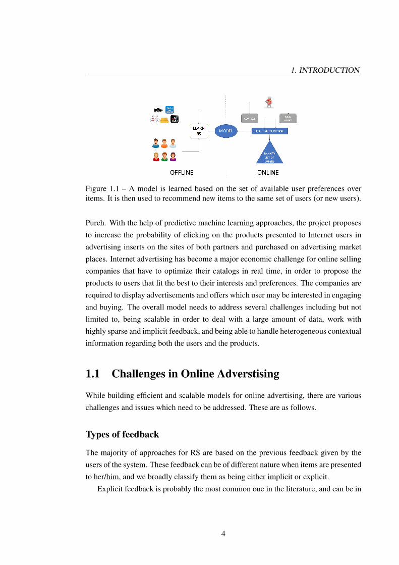
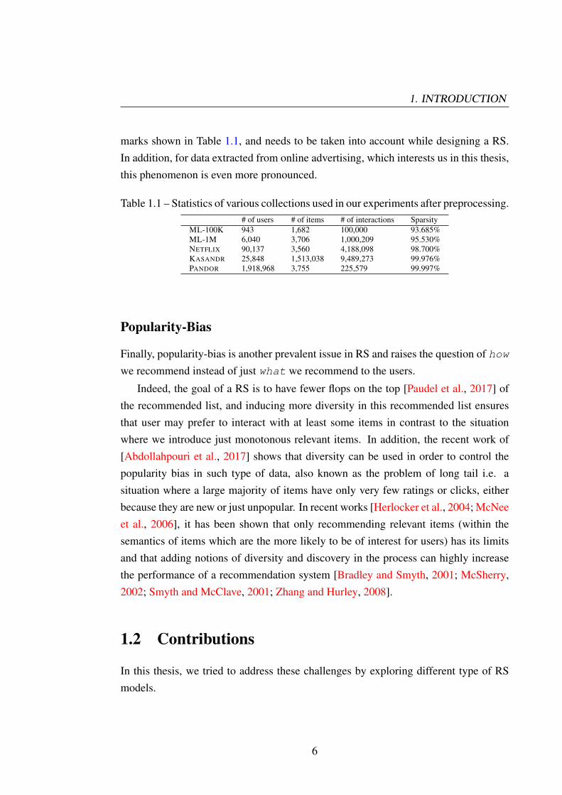


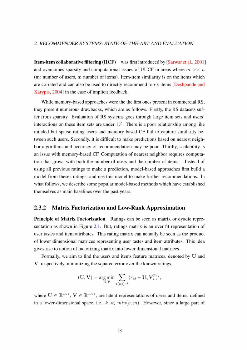
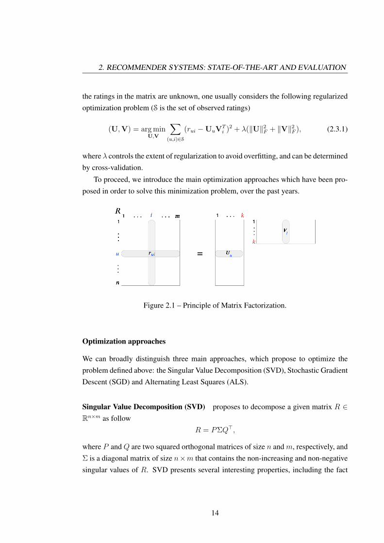


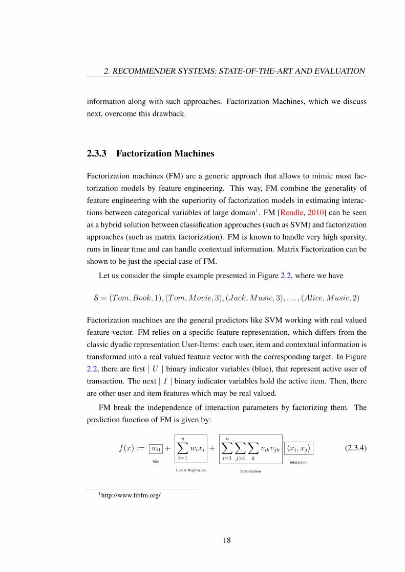
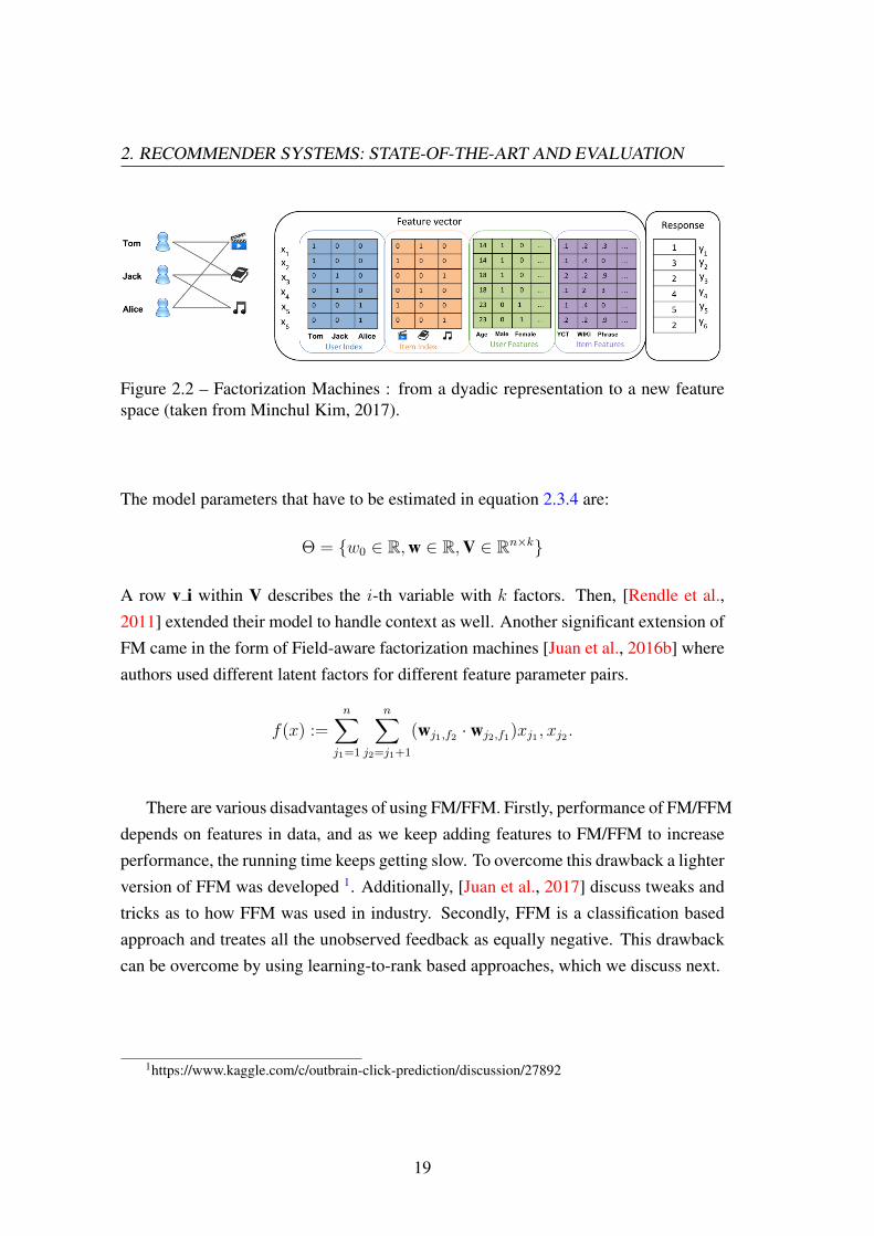


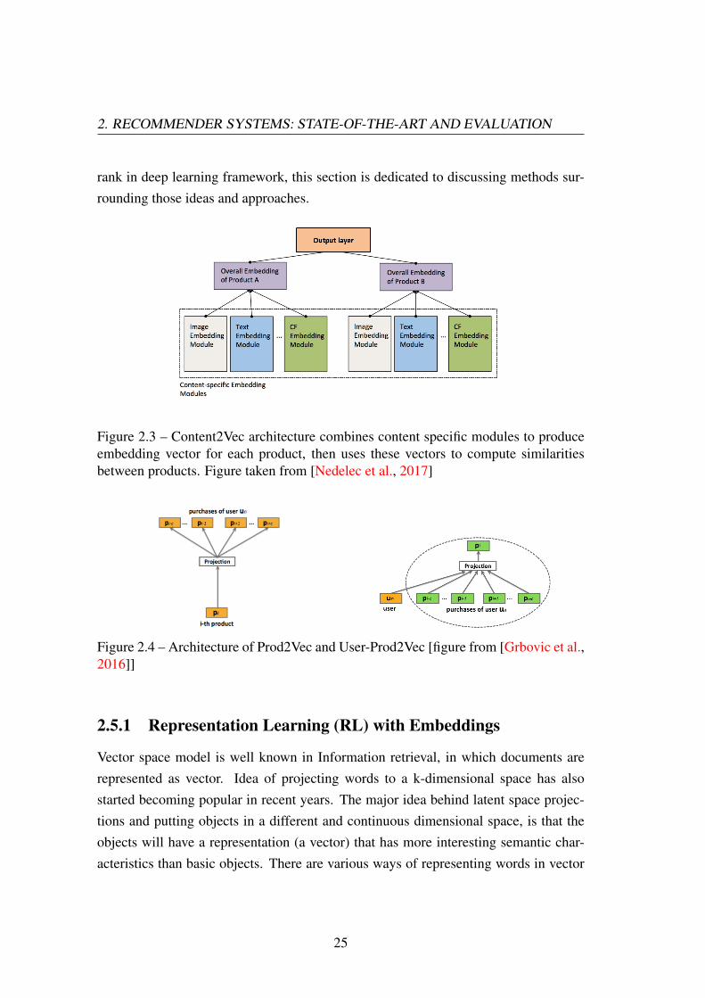

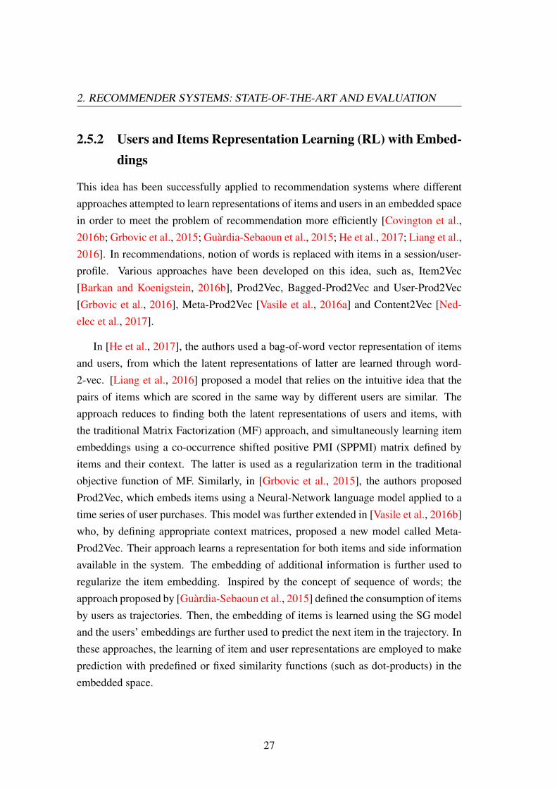


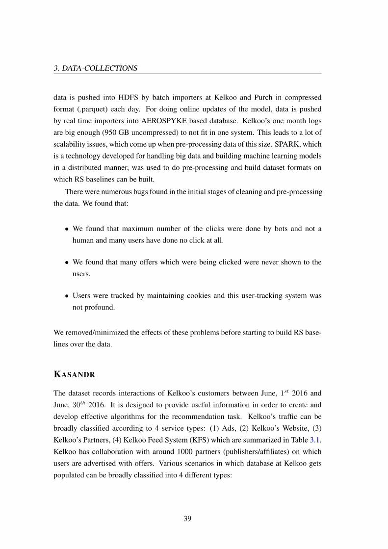


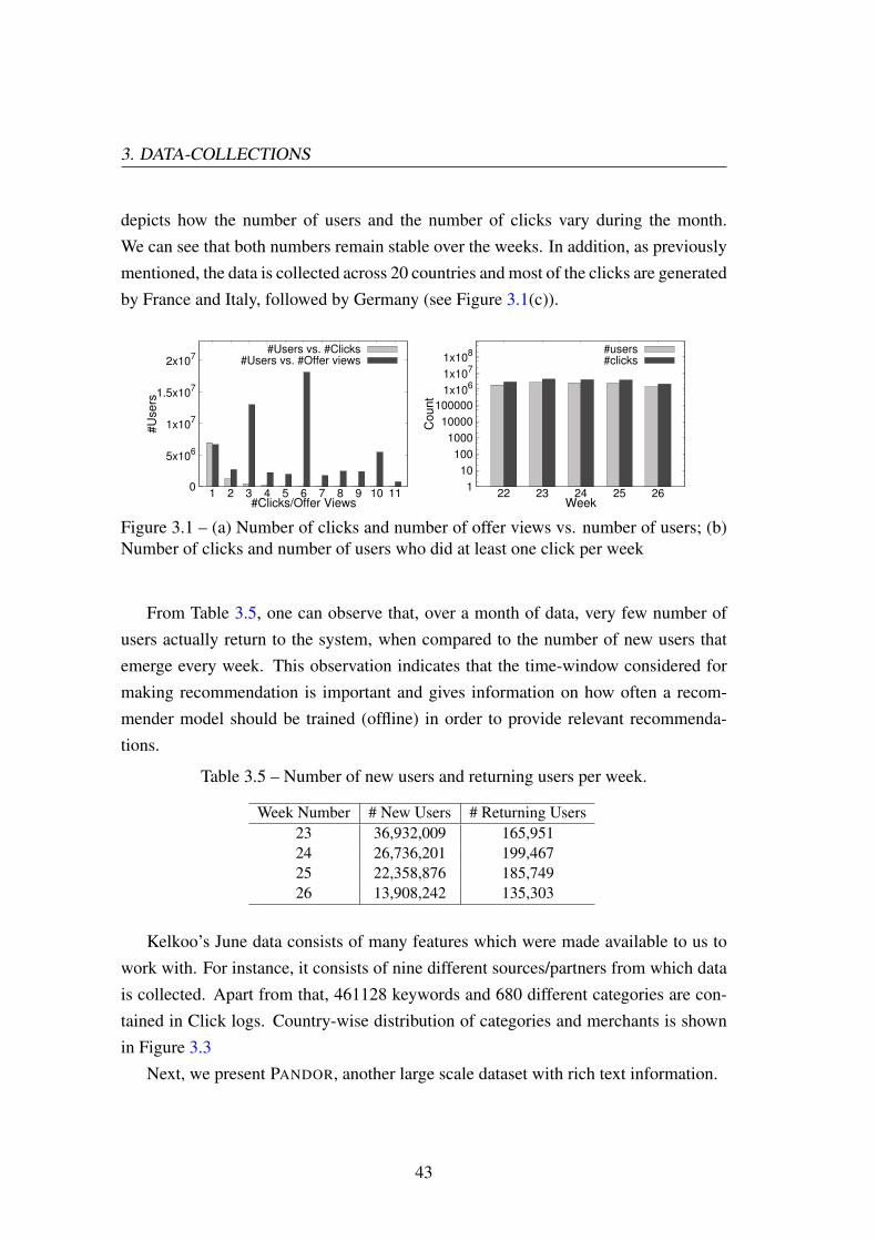
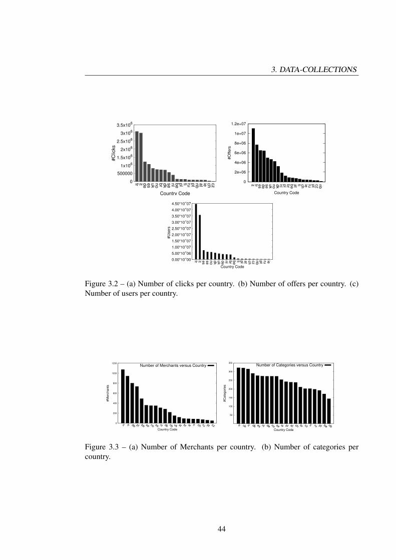

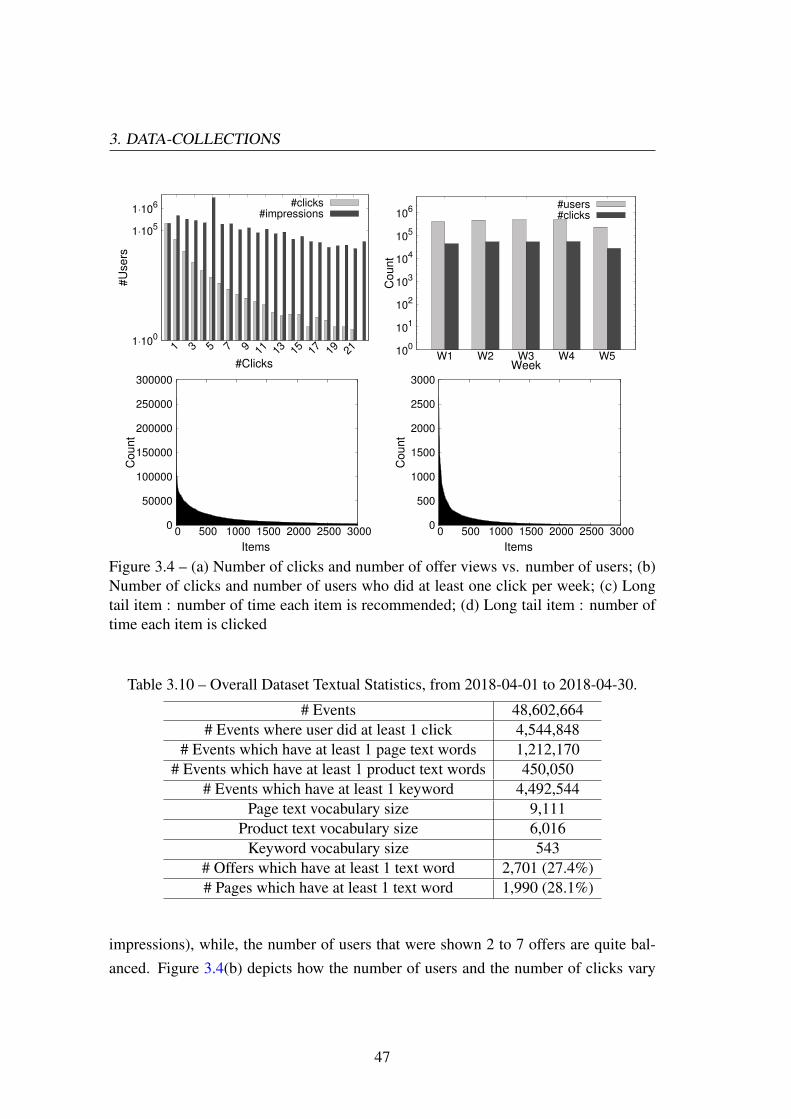

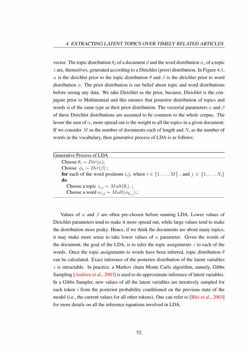
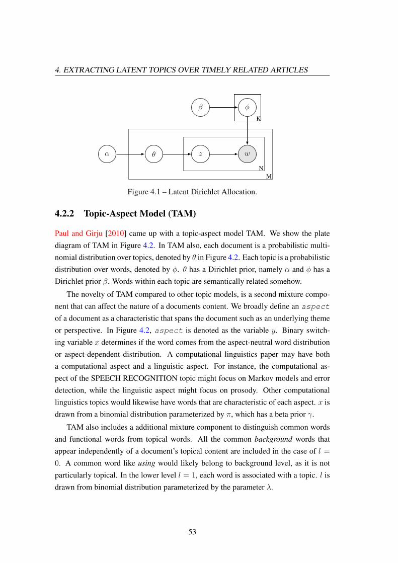


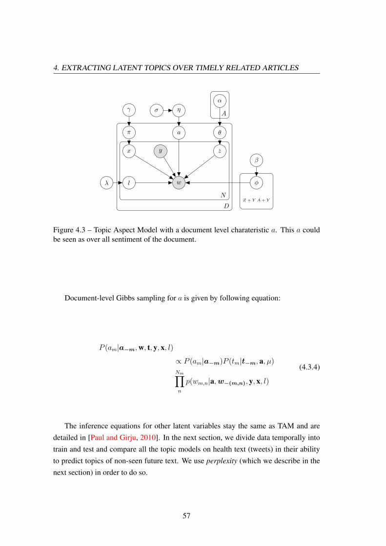
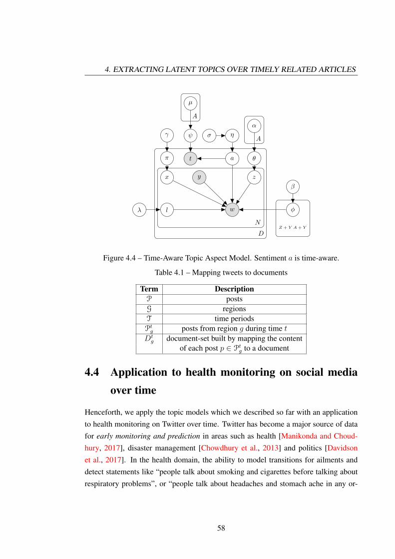

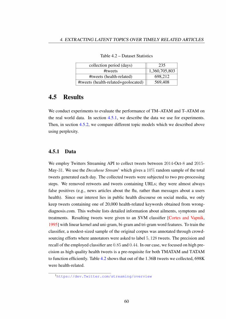


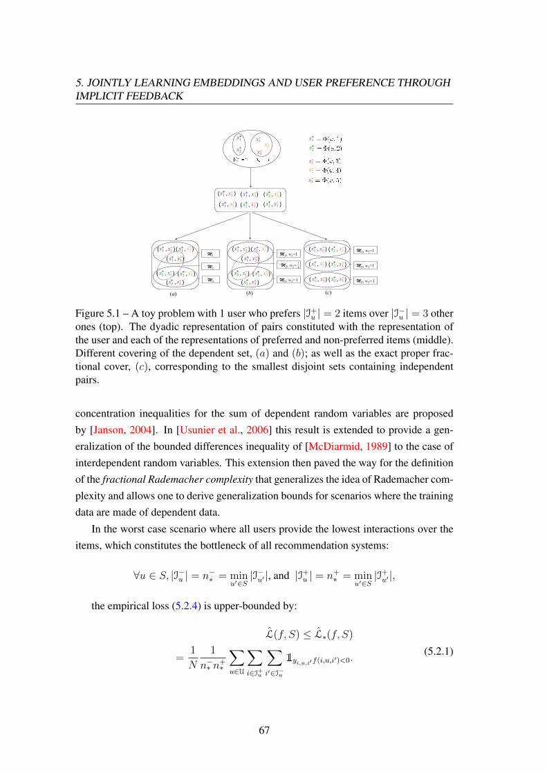


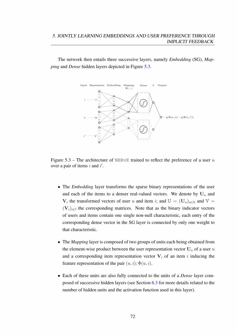


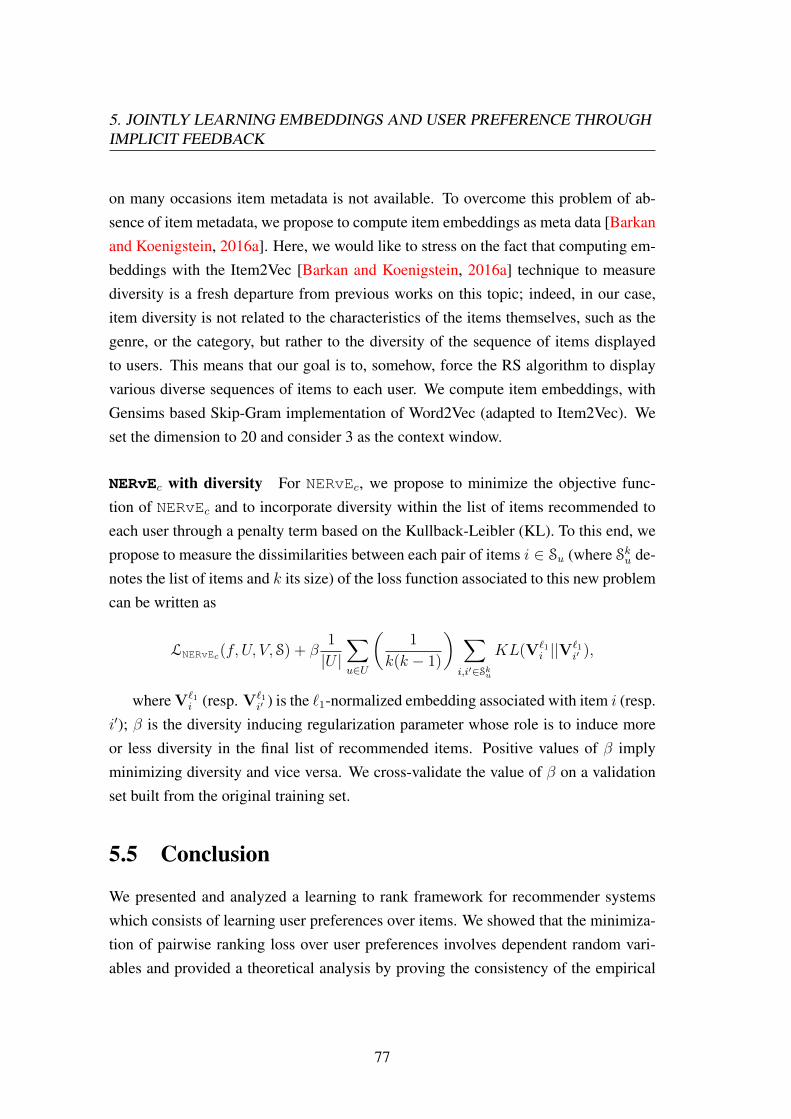


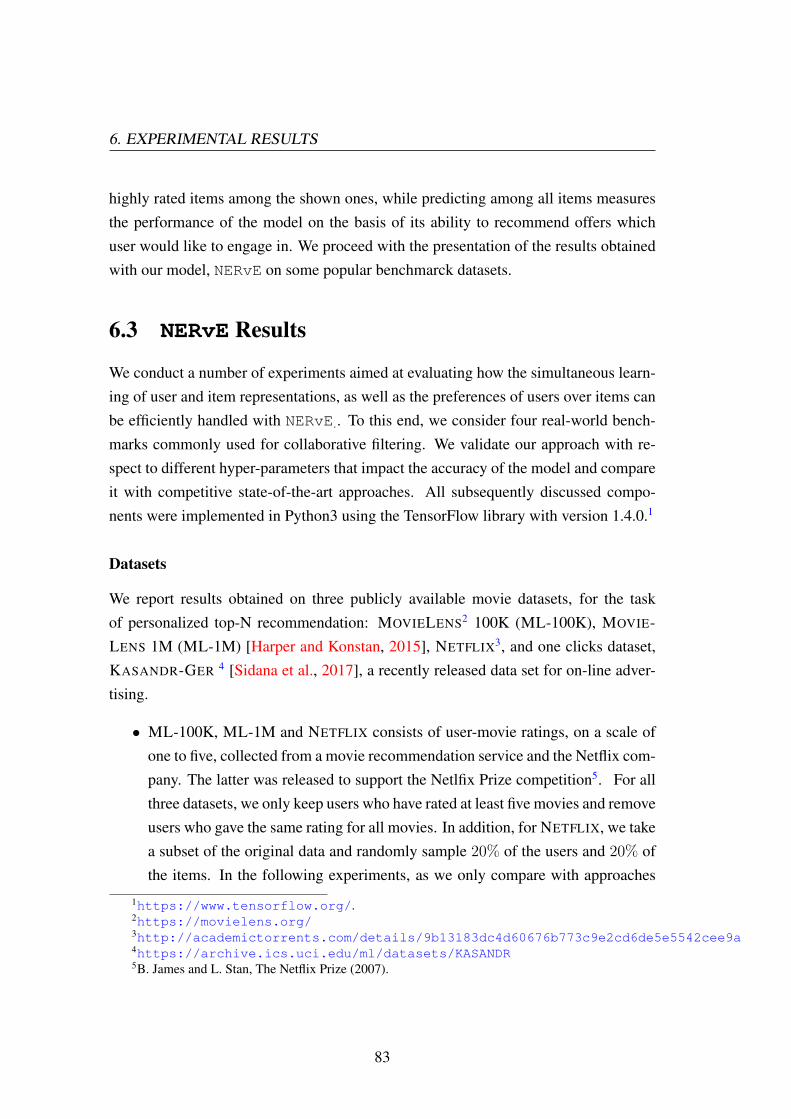
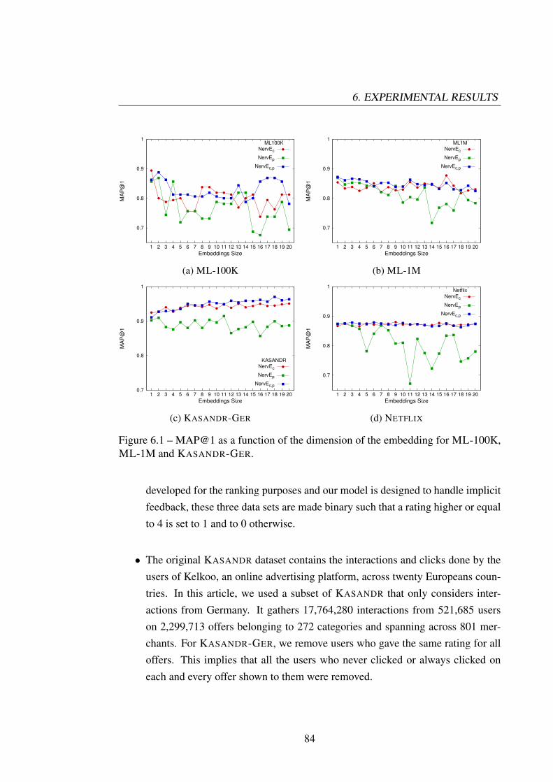
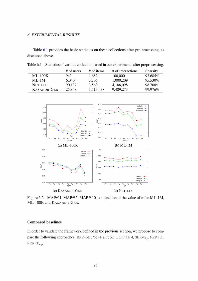
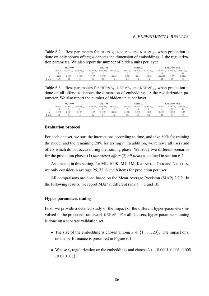


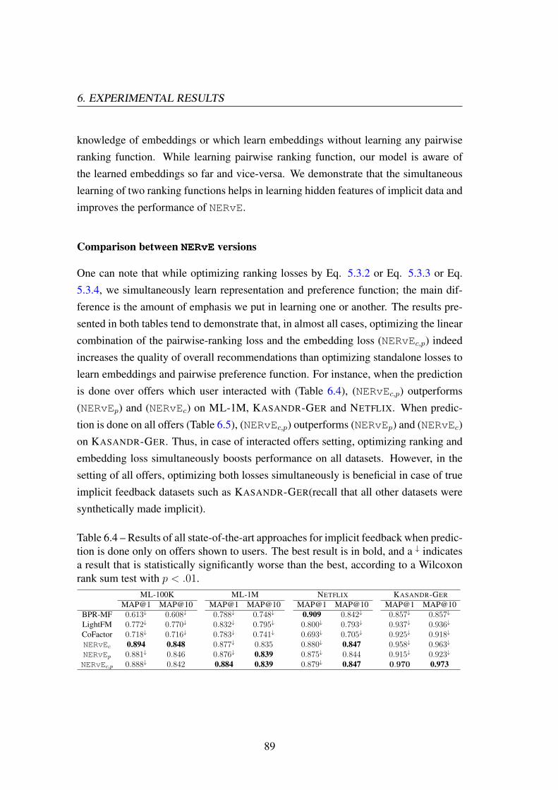


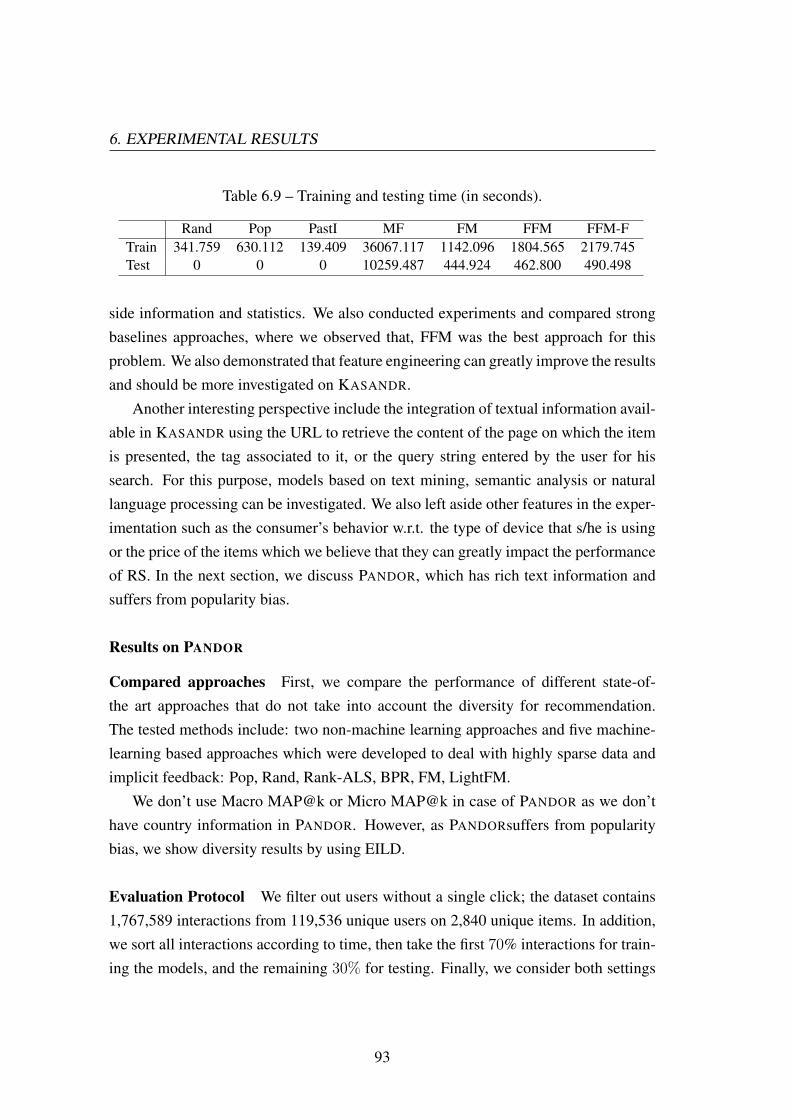
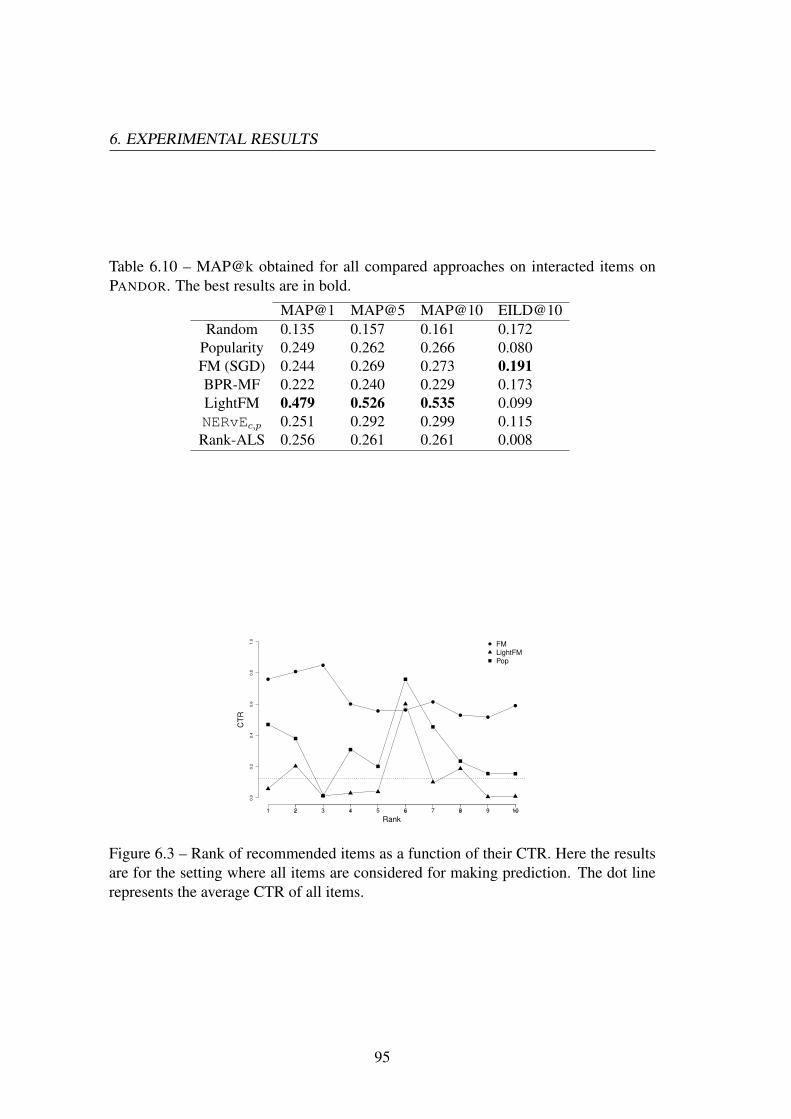
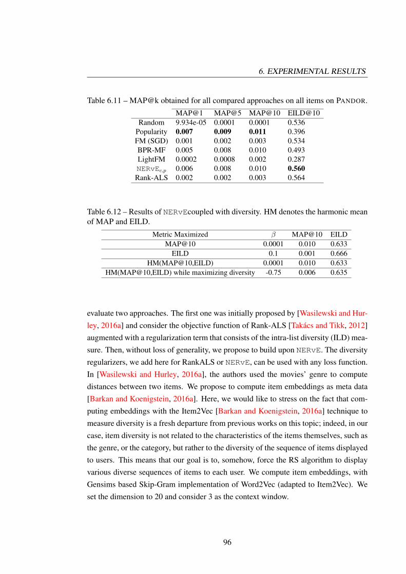
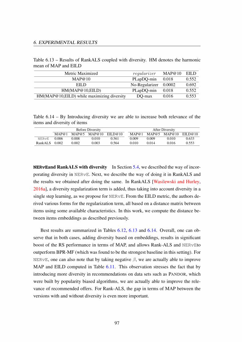
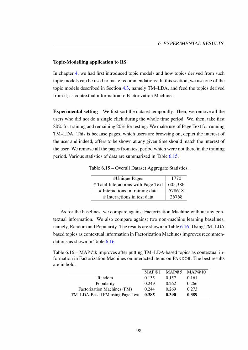


![Roadmap for technology and product development of airship by ml sidana et al[1]](https://static.documents.pub/doc/80x56/58a9fb8e1a28abec248b52b3/roadmap-for-technology-and-product-development-of-airship-by-ml-sidana-et-al1.jpg)


