SET Summary for Chesapeake Bay-MD Reserve Page 1

Summary for Outreach Wetland Surface Elevation Table (SET) Data

for Chesapeake Bay-MD National Estuarine Research Reserve (CBM)

Maryland, 2010-2016

To learn more about project, project team, and related products visit: nerrssciencecollaborative.org/project/Cressman18

Contact: Kim Cressman, Grand Bay National Estuarine Research Reserve, kimberly.cressman@dmr.ms.gov

SET Outreach Tools 2020-02-26

This document is intended for use as an outreach tool to help National Estuarine Research Reserve (NERR) Education and Coastal Training Program staff present and describe information relating to Surface Elevation Table (SET) data. These products are output from a 2018-2019 NERRS Science Collaborative Catalyst Grant project nicknamed “SETr”.

Importance of Tidal Wetlands and Sea Level

Tidal wetlands are very important to coastal areas - they provide wildlife habitat, including nursery habitat for commercial and recreational fish species; are areas for recreational and economic opportunity; store carbon; and offer flood protection. There are a variety of tidal wetlands: submerged vegetation (such as eelgrass), marshes, forested swamps, and mangroves. The type of wetland in a given location is related to elevation and inundation (flooding) regime - how often the surface of the wetland is flooded by the tide, and the salinity of those tidal waters. For example, eelgrass meadows have lower elevations than marshes and are more frequently submerged. Many factors affect wetland elevation, including shallow surface components - such as organic matter buildup by plant roots and sediment deposits at the surface - and sub-surface components such as geologic uplift or subsidence. The data described here focus on changes due to shallow surface components.

Long term sea level rise (SLR) rates vary regionally due to processes such as subsidence, which causes increased relative SLR rates, or isostatic rebound from glaciation, which causes the land surface to rise and leads to a decrease in relative SLR. Even changes in ocean surface currents can affect sea levels observed at particular locations. Similarly, there is variability in changes to surface elevation of wetlands at both the local and regional level due to a variety of drivers, such as human disturbance, whether systems are ocean or river driven, inundation patterns, and plant community composition.

SET Summary for Chesapeake Bay-MD Reserve Page 2

Analyzing rates of marsh surface elevation change, in the context of local sea level changes, can help identify patterns to determine how resilient tidal wetlands across the nation are to SLR.

Background on SETs - National level

The “Sentinel Site Application 1” (SSAM-1) module of the NERR Sentinel Site Program integrates water level data, System-Wide Monitoring Program (SWMP) abiotic data, vegetation data, and elevation measurements, for the purpose of assessing the impacts of sea level change on tidal wetlands. Surface Elevation Table (SET) technology, a means of measuring changes to the height of the wetland substrate, is a widely implemented component of SSAM-1. In this project, previously collected NERRS SET data was analyzed to answer the question – are marsh surfaces keeping pace with sea level rise? Note that this is an analysis looking back through time; it is not a forecasting tool.

A Surface Elevation Table (SET) consists of two main parts: 1) a portable apparatus designed to attach to 2) a permanent sampling station. The permanent station consists of a rod driven into the ground as deeply as possible (point of refusal), to which a receiver was attached and permanently cast in a cement collar (referenced as #1 ‘SET mark’ in Figure 1). The portable SET apparatus consists of a vertical stand, which attaches to the receiver, and a horizontal arm that reaches out over the marsh surface. For measurements, the portable apparatus is temporarily attached to the SET receiver such that the arm is horizontally level. A long narrow pin of a known length (see #4 in Figure 1) is inserted vertically through each of nine holes drilled through the arm. The observer then measures the height of each pin above the arm (#3 in Figure 1). The arm is then moved to another one of the directions around the SET mark and the process is repeated. The arm has typically four (but as many as eight) possible orientations. This allows for a minimum of 36 measurements taken at any given SET.

SET Summary for Chesapeake Bay-MD Reserve Page 3

Figure 1. Example of a SET. Pin heights above the horizontal arm (A) are a proxy for the shape of the marsh surface (B) (adapted from Lynch et al. 2015).

Any descriptive information pertinent to the measurements at each pin is also recorded (e.g., mounds or divots on the substrate such as crab burrows, or the sediment surface being difficult to interpret due to the pin being located in water).

These measurements are repeated over time. Because of the stability of the SET mark, each pin is lowered to the surface in the same location, time after time. The measurement can be used to calculate where the surface is, and other measurements can relate it back to standard frameworks, such as local mean sea level. After several years, scientists can calculate a “rate of change” for the marsh surface. Is it getting higher, lower, or not changing?

Because tidal wetlands are so important to coastal areas, we especially want to know if the surface is growing quickly enough to keep up with sea level rise.

SET Summary for Chesapeake Bay-MD Reserve Page 4

Figure 2. SET apparatus installed and observer taking measurement with meter stick atop the SET arm (photo credit Hudson River NERR).

Background on SETs - Reserve level

Each reserve is in charge of its own SET data. As part of the SETr project, 15 reserves sent their data files to the project team, and each was reworked into the same data format. Because of this standardization, we can generate several tables and graphs that look the same for each reserve; but each one uses the individual reserve’s data! This document contains data for your reserve.

Pin measurements are stored in a spreadsheet that contains columns for the SET ID, date of measurement, measured height of the pin above the SET apparatus arm, and QA/QC codes (concise codes to mark common issues with a pin measurement). A separate spreadsheet contains metadata: higher-level information about the SETs themselves, such as its exact location (latitude and longitude), the most common vegetation type around the SET, typical salinity in the nearby water body, and other general information.

Information from both spreadsheets is pulled together to communicate about the SETs and how they are changing.

## Warning: The following SET IDs exist in your metadata, but not in your ## data. Output may not match what you expect.IPT1L, IPT1H, IPT2L, IPT2H, ## RRT3L, RRT3H, RRT4L, RRT4H, MT4L, MT4H, MT5L, MT5H, RRT1LS3, RRT1LS4, ## RRT1HS5, RRT2LS7, RRT2LS8

## Warning: Column `set_id`/`unique_set_id` joining factors with different ## levels, coercing to character vector

SET Summary for Chesapeake Bay-MD Reserve Page 5

Reserve-level context • Local rate of sea level change is 3.82 +/- 0.24 mm/yr.

• This rate is reported by Solomons Island, MD, NWLON station number 8577330 based on

data from 1937 to 2018. SET-level characteristics Setting

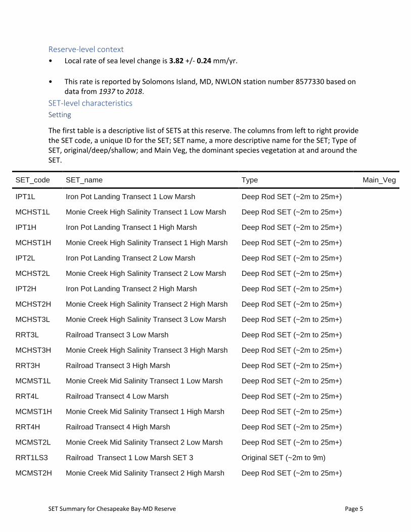
The first table is a descriptive list of SETS at this reserve. The columns from left to right provide the SET code, a unique ID for the SET; SET name, a more descriptive name for the SET; Type of SET, original/deep/shallow; and Main Veg, the dominant species vegetation at and around the SET.

SET_code SET_name Type Main_Veg

IPT1L Iron Pot Landing Transect 1 Low Marsh Deep Rod SET (~2m to 25m+)

MCHST1L Monie Creek High Salinity Transect 1 Low Marsh Deep Rod SET (~2m to 25m+)

IPT1H Iron Pot Landing Transect 1 High Marsh Deep Rod SET (~2m to 25m+)

MCHST1H Monie Creek High Salinity Transect 1 High Marsh Deep Rod SET (~2m to 25m+)

IPT2L Iron Pot Landing Transect 2 Low Marsh Deep Rod SET (~2m to 25m+)

MCHST2L Monie Creek High Salinity Transect 2 Low Marsh Deep Rod SET (~2m to 25m+)

IPT2H Iron Pot Landing Transect 2 High Marsh Deep Rod SET (~2m to 25m+)

MCHST2H Monie Creek High Salinity Transect 2 High Marsh Deep Rod SET (~2m to 25m+)

MCHST3L Monie Creek High Salinity Transect 3 Low Marsh Deep Rod SET (~2m to 25m+)

RRT3L Railroad Transect 3 Low Marsh Deep Rod SET (~2m to 25m+)

MCHST3H Monie Creek High Salinity Transect 3 High Marsh Deep Rod SET (~2m to 25m+)

RRT3H Railroad Transect 3 High Marsh Deep Rod SET (~2m to 25m+)

MCMST1L Monie Creek Mid Salinity Transect 1 Low Marsh Deep Rod SET (~2m to 25m+)

RRT4L Railroad Transect 4 Low Marsh Deep Rod SET (~2m to 25m+)

MCMST1H Monie Creek Mid Salinity Transect 1 High Marsh Deep Rod SET (~2m to 25m+)

RRT4H Railroad Transect 4 High Marsh Deep Rod SET (~2m to 25m+)

MCMST2L Monie Creek Mid Salinity Transect 2 Low Marsh Deep Rod SET (~2m to 25m+)

RRT1LS3 Railroad Transect 1 Low Marsh SET 3 Original SET (~2m to 9m)

MCMST2H Monie Creek Mid Salinity Transect 2 High Marsh Deep Rod SET (~2m to 25m+)

SET Summary for Chesapeake Bay-MD Reserve Page 6

SET_code SET_name Type Main_Veg

RRT1LS4 Railroad Transect 1 Low Marsh SET 4 Original SET (~2m to 9m)

MCMST3L Monie Creek Mid Salinity Transect 3 Low Marsh Deep Rod SET (~2m to 25m+)

RRT1HS5 Railroad Transect 1 High Marsh SET 5 Original SET (~2m to 9m)

MCMST3H Monie Creek Mid Salinity Transect 3 High Marsh Deep Rod SET (~2m to 25m+)

RRT2LS7 Railroad Transect 2 Low Marsh SET 7 Original SET (~2m to 9m)

RRT2LS8 Railroad Transect 2 Low Marsh SET 8 Original SET (~2m to 9m)

MT4L Mataponi Creek Transect 4 Low Marsh Deep Rod SET (~2m to 25m+)

MT4H Mataponi Creek Transect 4 High Marsh Deep Rod SET (~2m to 25m+)

MT5L Mataponi Creek Transect 5 Low Marsh Deep Rod SET (~2m to 25m+)

MT5H Mataponi Creek Transect 5 High Marsh Deep Rod SET (~2m to 25m+)

Sampling Information

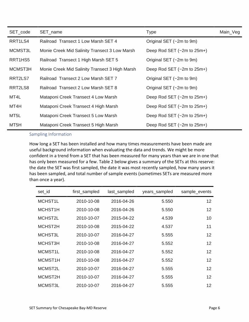
How long a SET has been installed and how many times measurements have been made are useful background information when evaluating the data and trends. We might be more confident in a trend from a SET that has been measured for many years than we are in one that has only been measured for a few. Table 2 below gives a summary of the SETs at this reserve: the date the SET was first sampled, the date it was most recently sampled, how many years it has been sampled, and total number of sample events (sometimes SETs are measured more than once a year).

set_id first_sampled last_sampled years_sampled sample_events

MCHST1L 2010-10-08 2016-04-26 5.550 12

MCHST1H 2010-10-08 2016-04-26 5.550 12

MCHST2L 2010-10-07 2015-04-22 4.539 10

MCHST2H 2010-10-08 2015-04-22 4.537 11

MCHST3L 2010-10-07 2016-04-27 5.555 12

MCHST3H 2010-10-08 2016-04-27 5.552 12

MCMST1L 2010-10-08 2016-04-27 5.552 12

MCMST1H 2010-10-08 2016-04-27 5.552 12

MCMST2L 2010-10-07 2016-04-27 5.555 12

MCMST2H 2010-10-07 2016-04-27 5.555 12

MCMST3L 2010-10-07 2016-04-27 5.555 12

SET Summary for Chesapeake Bay-MD Reserve Page 7

set_id first_sampled last_sampled years_sampled sample_events

MCMST3H 2010-10-07 2016-04-27 5.555 12

Graphs Changes through time at individual SETs Single SET

Figure 3 is a graph of data from a single SET at this reserve. The x-axis shows measurement date; as we move from left to right in the graph, we move through time. The y-axis shows change since the first measurement (often referred to as “baseline”). Remember how we said there are 36 measurements on each date? You’re only seeing one point on each date in this graph, because 36 measurements is a lot! For simplicity, all 36 pin heights for a date have been averaged together.

Is the marsh surface getting higher, lower, or staying the same at this SET?

Figure 3. Average marsh height at one SET over time, as compared to the first reading.

Now, let’s add a line, from a statistical procedure called linear regression. For most SETs, a line is a useful simplification of the data. The data points bounce around a bit, but may still show that the marsh surface is changing over time. A linear regression takes all of this information and condenses it, mathematically, in ways that we can use to compare different sites. The slope of the line, in mm/year, gives us a general idea of how quickly the surface at a SET is changing. We refer to this slope as the rate of elevation change at the SET.

SET Summary for Chesapeake Bay-MD Reserve Page 8

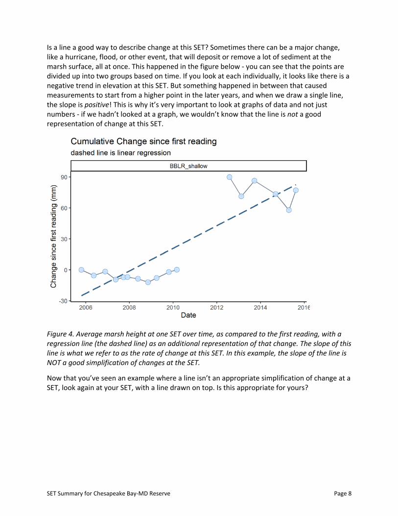
Is a line a good way to describe change at this SET? Sometimes there can be a major change, like a hurricane, flood, or other event, that will deposit or remove a lot of sediment at the marsh surface, all at once. This happened in the figure below - you can see that the points are divided up into two groups based on time. If you look at each individually, it looks like there is a negative trend in elevation at this SET. But something happened in between that caused measurements to start from a higher point in the later years, and when we draw a single line, the slope is positive! This is why it’s very important to look at graphs of data and not just numbers - if we hadn’t looked at a graph, we wouldn’t know that the line is not a good representation of change at this SET.

Figure 4. Average marsh height at one SET over time, as compared to the first reading, with a regression line (the dashed line) as an additional representation of that change. The slope of this line is what we refer to as the rate of change at this SET. In this example, the slope of the line is NOT a good simplification of changes at the SET.

Now that you’ve seen an example where a line isn’t an appropriate simplification of change at a SET, look again at your SET, with a line drawn on top. Is this appropriate for yours?

SET Summary for Chesapeake Bay-MD Reserve Page 9

Figure 5. Average marsh height at one SET over time, as compared to the first reading, with a regression line (the dashed line) as an additional representation of that change. The slope of this line is what we refer to as the rate of change at this SET.

What we really want to know is, how does the slope of that line compare to the rate (slope) of sea level change? Is one steeper than the other? In the next graph (Figure 5), we add a red line to represent change in sea level, based on the long-term rate calculated from a nearby tide station, as described earlier.

SET Summary for Chesapeake Bay-MD Reserve Page 10

Figure 6. Average marsh surface height at one SET over time, as compared to the first reading. The solid blue line is a linear regression of the SET data, and the red line shows the rate of sea level change.

Finally, we simplify a bit by removing the points themselves, keeping only the lines (Figure 6). It will become clear why we needed to simplify when we put all the SETs from this reserve together in one graphic.

SET Summary for Chesapeake Bay-MD Reserve Page 11

Figure 7. Average marsh surface height at one SET over time, as compared to the first reading. Gray line represents the data; the solid blue line is a linear regression of the data; the red line shows the rate of sea level change.

All SETs at this reserve

Here is a birds-eye view of all SETs at this reserve! Does it look like SETs at this reserve are generally keeping up with sea level rise? (Are the blue lines steeper than the red lines?)

SET Summary for Chesapeake Bay-MD Reserve Page 12

Figure 8. Average marsh surface height at each of this reserve’s SETs over time, as compared to each SET’s first reading. Each panel is one SET, with a gray line for the data, a solid blue line as a linear regression of the data, and a red line showing the rate of sea level change.

Comparisons to 0 and SLR

In this section, we’ll look at how the rate of marsh surface change compares to 0 (i.e. no change in surface elevation) and to local sea level change. We’ll start simple; with a gray vertical line at 0, a blue vertical line at the local rate of sea level rise (SLR), and a dot to represent the rate of change at each SET (rate of change increases from left to right on the x-axis).

Note - the rate of change at each SET can be:

• lower than 0: losing elevation

• higher than 0, but lower than SLR: gaining elevation but not as fast as the sea level is rising

SET Summary for Chesapeake Bay-MD Reserve Page 13

• higher than SLR: rate of elevation gain is exceeding local sea level rise rates

Figure 9. Summary graph of the rate of marsh surface elevation change at each SET.

Describing uncertainty

Of course, these calculated rates have some associated uncertainty. Here, we represent that with “whiskers” to show 95% confidence intervals. The wider the confidence interval is (whiskers are further apart), the less certain we are about the calculations:

SET Summary for Chesapeake Bay-MD Reserve Page 14

Figure 10. Summary graph of the rate of marsh surface elevation change at each SET, with whiskers to indicate 95% confidence intervals.

And: the calculated rate of sea level change ALSO has some associated uncertainty. Here, that is represented by light blue shading:

SET Summary for Chesapeake Bay-MD Reserve Page 15

Figure 11. Summary graph of the rate of marsh surface elevation change at each SET, with whiskers to indicate 95% confidence intervals for the SETs and shading to represent a 95% confidence interval for sea level change.

Now we’ll do the same building up, with a twist. Different plant communities may show different patterns in change over time. If vegetation information for the SETs was provided in the metadata document, it will be represented in the following graphs by coloring points by that dominant vegetation. If this information was not provided, figures 12-14 will not be generated.

Some questions we can answer from this graph:

1. Are most of the SETs at your reserve showing trends that are greater than 0 but less than sea level change (e.g. to the left of the blue shading?)

2. Are the SETs within a similar dominant vegetation community showing similar trends to each other?

3. How do the trends between dominant vegetation communities compare to each other? Are some vegetation communities gaining or losing elevation more quickly than others?

4. What does it mean when the whiskers (confidence intervals) on the SET data overlap the variability in SLR data (blue band)?

SET Summary for Chesapeake Bay-MD Reserve Page 16

On a map

Here we display SET locations on a map, with color-coded arrows to represent the rate of elevation change at a SET compared to either 0 (Figure 14) or to long-term sea level change (Figure 15).

Where are the changes happening within the reserve? Do you see any spatial patterns? What could be the reasons for these, based on what you know about the landscape of your reserve?

Compared to 0

First, are the SETs generally gaining or losing elevation? And does location - near the seaward edge of the marsh vs. upslope - matter? We can determine this by comparing each SET’s rate of elevation change (the slope of the linear regression in the first set of graphs) to 0. Up arrows depict SETs with positive rates of change - meaning increasing elevation - and down arrows show negative rates of change - decreasing elevation. If the arrows are red or blue, this means that 0 was not inside the confidence interval for that SET, and we are confident that the change at that SET is not 0 (meaning the elevation is changing). If the arrows are gray, we would not confidently claim a difference from 0.

Figure 15. Map of this reserve, showing how the rate of elevation change at each SET compares to 0.

Compared to SLR

The map below is similar to that above, but:

SET Summary for Chesapeake Bay-MD Reserve Page 17

• An up arrow represents a SET where the rate of elevation change (represented as a point in the dot-and-whisker graphs above) is higher than the rate of sea level change (the vertical blue line from those graphs), and a down arrow represents a SET where the rate of elevation change is lower than the rate of sea level change.

• Instead of asking “is 0 inside the confidence interval for each SET”, we ask if the confidence interval for sea level change overlaps the confidence interval for a SET - do the whiskers overlap the blue shading? It’s important to note for more science-minded audiences that this is not the same as the formal hypothesis tests we learned about in introductory statistics. We are comparing confidence intervals to get a general idea of how these different rates of change relate to each other.

– If the confidence intervals do not overlap, the arrows are red or blue and we would be confident saying the SET is changing at a different rate (faster or slower) than sea level is changing.

– If the confidence intervals do overlap, the arrow is gray and we are not confident that there is a difference between the SET’s rate of elevation change and that of sea level.

Figure 16. Map of this reserve, showing how the rate of elevation change at each SET compares to the rate of long-term sea level change.

Studying the maps for a while may allow you to see patterns that weren’t clear from the tables or graphs alone. What kinds of questions do you have about marsh elevation change after

SET Summary for Chesapeake Bay-MD Reserve Page 18

looking at these depictions of SET data? Can you think of any other factors that might influence this change, or help you interpret what you’ve seen here?