100
September 2013 I www.epa.gov/hfstudy Summary of the Technical Workshop on Water Acquisition Modeling: Assessing Impacts Through Modeling and Other Means June 4, 2013

September 2013 I www.epa.gov/hfstudy
Summary of the Technical Workshop on Water
Acquisition Modeling: Assessing Impacts Through Modeling and Other Means
June 4, 2013

EPA’s Study of the Potential Impacts of Hydraulic Fracturing on Drinking Water Resources: Summary of June 4, 2013, Technical Workshop on Water Acquisition Modeling: Assessing Impacts Through Modeling and Other Means
ii
Disclaimer
This report was prepared by EPA with assistance from Eastern Research Group, Inc., an EPA
contractor, as a general record of discussions during the June 4, 2013, technical workshop on
wastewater treatment and related modeling. The workshop was held to inform EPA’s Study of
the Potential Impacts of Hydraulic Fracturing on Drinking Water Resources. The report
summarizes the presentations and facilitated discussions on the workshop topics and is not
intended to reflect a complete record of all discussions. All statements and opinions expressed
represent individual views of the invited participants; there was no attempt to reach consensus on
any of the technical issues being discussed. Except as noted, none of the statements in the report
represent analyses or positions of EPA.
Mention of trade names or commercial products does not constitute endorsement or
recommendations for use.

EPA’s Study of the Potential Impacts of Hydraulic Fracturing on Drinking Water Resources: Summary of June 4, 2013, Technical Workshop on Water Acquisition Modeling: Assessing Impacts Through Modeling and Other Means
iii
Table of Contents
Meeting Agenda ........................................................................................................................1
List of Meeting Participants .....................................................................................................3
Introduction...............................................................................................................................5
Summary of Presentations for Session 1: Data on Water Acquisition and Water
Recycling/Reuse.........................................................................................................................6
Summary of Discussions Following Session 1: Data on Water Acquisition and Water
Recycling/Reuse.........................................................................................................................9
Summary of Presentations for Session 2: Hydraulic Fracturing Water Acquisition and
Water Availability Modeling Approaches .............................................................................. 12
Summary of Discussions Following Session 2: Hydraulic Fracturing Water Acquisition and
Water Availability Modeling Approaches .............................................................................. 14
Concluding Remarks............................................................................................................... 17
Appendix A. Extended Abstracts from Session 1: Data on Water Acquisition and Water
Recycling/Reuse.................................................................................................................... A-1
Water Acquisition: Analysis of Existing Data .................................................................... A-2
Sources of Data for Quantifying Hydraulic-Fracturing Water Use in Texas ....................... A-6
Water Acquisition for Unconventional Natural Gas Development Within the Susquehanna
River Basin .......................................................................................................................A-16
Recycling and Reuse of Produced Water to Reduce Freshwater Use in Hydraulic Fracturing
Operations ........................................................................................................................A-20
Appendix B. Extended Abstracts from Session 2: Current and Future Trends in Hydraulic
Fracturing Wastewater Management .................................................................................. B-1
Evaluating Scenarios of Potential Impact of Water Acquisition for Hydraulic Fracturing .... B-2
Mapping Water Availability and Cost in the Western United States .................................... B-6
Integrated, Collaborative Water Research in Western Canada ........................................... B-21
Appendix C. Poster Abstracts ............................................................................................. C-1
A Simulation Framework for Integrated Water and Energy Resource Planning ................... C-2
Utilizing Produced Water and Hydraulic Fracturing Flowback as a New Water Resource . C-13

EPA’s Study of the Potential Impacts of Hydraulic Fracturing on Drinking Water Resources: Summary of June 4, 2013, Technical Workshop on Water Acquisition Modeling: Assessing Impacts Through Modeling and Other Means
1
Meeting Agenda
Technical Workshop on Water Acquisition Modeling:
Assessing Impacts Through Modeling and Other Means
June 4, 2013
US EPA Conference Center at One Potomac Yards
Arlington, VA
8:00 am Registration/Check-in
8:30 am Welcome and Introductions ............................................................................ Ramona Trovato, US EPA
8:40 am Opening Remarks ................................................................... Glenn Paulson, Science Advisor, US EPA
8:45 am Purpose of Workshop ............................................................................................ Workshop Co-Chairs:
Jennifer Orme-Zavaleta, US EPA
James Richenderfer, Susquehanna River Basin Commission
Session 1: Data on Water Acquisition and Water Recycling/Reuse 8:55 am Panel Presentations:
EPA Data Review Projects ..................................................................... Andrew Gillespie, US EPA
Sources of Data to Understand Hydraulic Fracturing Water Use in Texas ..................... J-P Nicot, University of Texas at Austin
Water Acquisition for Unconventional Natural Gas Development Within the Susquehanna
River Basin ............................................. James Richenderfer, Susquehanna River Basin Commission
Recycling and Reuse of Produced Water to Reduce Freshwater Use in Hydraulic Fracturing
Operations........................................................... Matthew Mantell, Chesapeake Energy Corporation
Questions of Clarification
Break (10 minutes)
Facilitated discussion among workshop participants focusing on key questions:
What existing sources of data could be used to better understand the effects of hydraulic fracturing
water acquisition on water system availability?
What are key attributes of a scientifically robust approach to measuring and monitoring hydraulic
fracturing water use and disposition?
What is the current state of industry practice with respect to recycling/reusing water for hydraulic
fracturing operations?
What are the long-term lifecycle implications and regional trends of recycling/reusing water in
hydraulic fracturing operations?

EPA’s Study of the Potential Impacts of Hydraulic Fracturing on Drinking Water Resources: Summary of June 4, 2013, Technical Workshop on Water Acquisition Modeling: Assessing Impacts Through Modeling and Other Means
2
11:45 am Summary of Session 1 ........................................................................................... Workshop Co-Chairs
12:00 pm Lunch and Poster Session
Session 2: Hydraulic Fracturing Water Acquisition and Water Availability Modeling Approaches
1:30 pm Panel Presentations:
Evaluating Scenarios of Potential Impact of Water Acquisition ............ Stephen Kraemer, US EPA
Mapping Water Availability and Cost in the Western United States ....................Vincent Tidwell,
Sandia National Laboratory
Integrated, Collaborative Water Research in Western Canada....... Ben Kerr, Foundry Spatial Ltd.
Water Need and Availability for Hydraulic Fracturing in the Bakken Formation, Eastern
Montana .................................................................... Mitchell Plummer, Idaho National Laboratory
Questions of Clarification
Break (10 minutes)
Facilitated discussion among workshop participants focusing on key questions:
What would a more generalized, conceptual model look like for assessing hydraulic fracturing
impacts in different areas of the US and at different scales?
What factors should be included in a generalized model?
3:45 pm Summary of Session 2 ........................................................................................... Workshop Co-Chairs
3:55 pm Closing Remarks ............................................................................................ Ramona Trovato, US EPA
4:00 pm Adjourn
Poster Session A Simulation Framework for Integrated Water and Energy Resource Planning
Robert Jeffers, Idaho National Laboratory
Utilizing Produced Water and Hydraulic Fracturing Flowback as a New Water Resource David Stewart, Energy Water Solutions, LLC
EPA’s Study of the Potential Impacts of Hydraulic Fracturing on Drinking Water Resources: Summary of June 4, 2013, Technical Workshop on Water Acquisition Modeling: Assessing Impacts Through Modeling and Other Means
3
List of Meeting Participants Bruce Baizel Earthworks
Michael G. Baker
Ohio Environmental Protection Agency
Lily Baldwin
Chevron Energy Technology Company
Laura Belanger
Western Resource Advocates
Lisa Biddle
US EPA Office of Water
Jeanne Briskin
US EPA Office of Research and
Development
Thomas Chambers
Southwestern Energy Company
Corrie Clark
Argonne National Laboratory
Bruce Curtis
Kleinfelder, Inc.
R. Jeffrey Davis
Cardno ENTRIX
Michael Dunkel
Pioneer Natural Resources
H. Thomas Fridirici
Pennsylvania Department of Environmental
Protection
Andrew Gillespie*
US EPA ORD/National Exposure Research
Laboratory
Rowlan Greaves
Southwestern Energy Company
Christopher Harto
Argonne National Laboratory
David Hollas
Halliburton Energy Services, Inc.
Robert Jeffers
Idaho National Laboratory
Stephen Jester
ConocoPhillips
Mary Kang
Princeton University
Ben Kerr*
Foundry Spatial Ltd.
Stephen Kraemer*
US EPA ORD/National Exposure Research
Laboratory
Dan Luecke
Consultant
Matthew Mantell*
Chesapeake Energy Corporation
Mike Mathis
Chesapeake Energy Corporation
Lisa Matthews
US EPA Office of Research and Development
Jan Matuszko
US EPA Office of Water
* Presenter

EPA’s Study of the Potential Impacts of Hydraulic Fracturing on Drinking Water Resources: Summary of June 4, 2013, Technical Workshop on Water Acquisition Modeling: Assessing Impacts Through Modeling and Other Means
4
Adam McDonough
American Water Works Service Company, Inc.
Kenneth Nichols
CH2M HILL
Jean-Philippe Nicot*
University of Texas at Austin
Jennifer Orme-Zavaleta (co-chair)
US EPA ORD/National Exposure Research
Laboratory
Glenn Paulson US EPA, Science Advisor
Mitchell Plummer*
Idaho National Laboratory
James Richenderfer* (co-chair)
Susquehanna River Basin Commission
Andrew Ross
Colorado Department of Public Health and
Environment
Chantal Savaria
Savaria Experts-Conseils Inc.
Kelly Smith
US EPA ORD/National Risk Management
Research Laboratory
Daniel Soeder
US Department of Energy
David Stewart
Energy Water Solutions, LLC
Kate Sullivan
US EPA ORD/National Exposure Research
Laboratory
Patrick Sullivan
Aquilogic, Inc.
Brenan Tarrier
New York State Department of Environmental
Conservation
Joel Thompson
Stantec, Inc.
Amy Tidwell
ExxonMobil Upstream Research Company
Vincent Tidwell*
Sandia National Laboratories
D. Steven Tipton
Newfield Exploration Company
Ramona Trovato
US EPA Office of Research and Development
Denise Tuck
Halliburton Energy Services, Inc.
Jim Weaver
US EPA ORD/National Risk Management
Research Laboratory
W. Joshua Weiss
Hazen and Sawyer, P.C.
Lloyd Wilson
New York State Department of Health
* Presenter

EPA’s Study of the Potential Impacts of Hydraulic Fracturing on Drinking Water Resources: Summary of June 4, 2013, Technical Workshop on Water Acquisition Modeling: Assessing Impacts Through Modeling and Other Means
5
Introduction
At the request of Congress, the U.S. Environmental Protection Agency (EPA) is conducting a
study to better understand the potential impacts of hydraulic fracturing on drinking water
resources. The scope of the research includes the full cycle of water associated with hydraulic
fracturing activities. In the study, each stage of the water cycle is associated with a primary
research question:
Water acquisition: What are the possible impacts of large volume water withdrawals
from ground and surface waters on drinking water resources?
Chemical mixing: What are the possible impacts of hydraulic fracturing fluid surface
spills on or near well pads on drinking water resources?
Well injection: What are the possible impacts of the injection and fracturing process on
drinking water resources?
Flowback and produced water: What are the possible impacts of surface spills on or
near well pads of flowback and produced water on drinking water resources?
Wastewater treatment and waste disposal: What are the possible impacts of
inadequate treatment of hydraulic fracturing wastewaters on drinking water resources?
In 2013, EPA hosted a series of technical workshops related to its Study of the Potential Impacts
of Hydraulic Fracturing on Drinking Water Resources. The workshops included Analytical
Chemical Methods (February 25, 2013), Well Construction/Operation and Subsurface Modeling
(April 16–17, 2013), Wastewater Treatment and Related Modeling (April 18, 2013), Water
Acquisition Modeling (June 4, 2013) and Hydraulic Fracturing Case Studies (July 30, 2013). The
workshops were intended to inform EPA on subjects integral to enhancing the overall hydraulic
fracturing study, increasing collaborative opportunities and identifying additional possible future
research areas. Each workshop addressed subject matter directly related to the primary research
questions.
For each workshop, EPA invited experts with significant relevant and current technical
experience. Each workshop consisted of invited presentations followed by facilitated discussion
among all invited experts. Participants were chosen with the goal of maintaining balanced
viewpoints from a diverse set of stakeholder groups including industry; nongovernmental
organizations; other federal, state and local governments; tribes; and the academic community.
The fourth workshop, Water Acquisition Modeling: Assessing Impacts Through Modeling and
Other Means, was co-chaired by Dr. Jennifer Orme-Zavaleta (EPA) and Dr. James Richenderfer
(Susquehanna River Basin Commission [SRBC]). A morning session addressed Data on Water
Acquisition and Water Recycling/Reuse while the afternoon session focused on Hydraulic
Fracturing Water Acquisition and Water Availability Modeling Approaches. In addition, several
experts shared technical knowledge during a poster session (see Appendix C of this report).

EPA’s Study of the Potential Impacts of Hydraulic Fracturing on Drinking Water Resources: Summary of June 4, 2013, Technical Workshop on Water Acquisition Modeling: Assessing Impacts Through Modeling and Other Means
6
Summary of Presentations for Session 1: Data on Water Acquisition and Water Recycling/Reuse
Susan Hazen, Hazen Consulting and Support Services, opened the workshop. She noted that
EPA was looking for individual participants’ frank input and opinion and was not trying to reach
consensus on the topics; the workshop was not being held under the rules of the Federal
Advisory Committee Act (FACA). Ramona Trovato, Associate Assistant Administrator of
EPA’s Office of Research and Development, and Dr. Glenn Paulson, Science Advisor to the
EPA Administrator, welcomed the participants and thanked them for contributing their
knowledge and experience to help answer the water acquisition research questions in EPA’s
drinking water study. Workshop Co-Chairs Dr. Jennifer Orme-Zavaleta, Director of EPA’s
National Exposure Research Laboratory, and Dr. James Richenderfer, Director of Technical
Programs for the Susquehanna River Basin Commission, also welcomed the participants. They
explained that the purpose of the workshop was to hear different stakeholders’ perspectives and
to better understand industry practices and how they are changing.
Dr. Andrew Gillespie, EPA National Exposure Research Laboratory, provided an overview of
EPA’s drinking water study approach to studying the water acquisition stage of the water cycle,
and described EPA’s analysis of existing data about water acquisition for hydraulic fracturing
operations. He noted that the primary research question associated with the water acquisition
stage of the hydraulic fracturing water cycle is “What are the possible impacts of large volume
water withdrawals on drinking water resources?” The secondary research questions related to
water acquisition are:
How much water is used in hydraulic fracturing operations, and what are the sources of
this water?
How might water withdrawals affect short- and long-term water availability in an area
with hydraulic fracturing activity?
What are the possible impacts of water withdrawals for hydraulic fracturing operations on
local water quality?
Dr. Gillespie noted that hydraulic fracturing accounts for a very small fraction of the nation’s
annual water use (less than 0.1 percent). However, the impacts of withdrawal may not be visible
at a national scale or state scales. The potential for greater impacts may exist at the local level,
depending on such factors as the catchment area and distribution of hydraulic fracturing
operations in a given area, the local geology and hydrology, competing local water needs, and
climate and seasonal variations. Dr. Gillespie discussed some anecdotal evidence of increased
recycling/reuse of produced and flowback water, noting that participants in the April 4, 2013,
technical workshop on wastewater had discussed the importance of local conditions for recycling
and reuse, the potential for cost savings, and possible reduction in freshwater utilization. He then
described the existing data that EPA is analyzing to answer the research questions: scientific
literature, FracFocus data, information from nine service companies that hydraulically fractured
24,925 wells in 2009–2010, and well files from 331 oil and gas wells across the United States.

EPA’s Study of the Potential Impacts of Hydraulic Fracturing on Drinking Water Resources: Summary of June 4, 2013, Technical Workshop on Water Acquisition Modeling: Assessing Impacts Through Modeling and Other Means
7
Dr. Jean-Philippe Nicot, Bureau of Economic Geology, University of Texas at Austin,
discussed sources of data for understanding hydraulic fracturing water use in Texas. Data on
hydraulic fracturing water use in Texas are readily available from operators themselves or from
the regulating agency, the Railroad Commission of Texas (RRC). In Texas, hydraulic fracturing
occurs in oil and gas plays, shales, and tight formations. In 2011, there was an increase in
completion water use in oil/liquid plays because of the decrease in gas prices. Dr. Nicot noted
that operators have to report completion water use to the RRC; several private vendors make
these data available in a useful form. He described the process he uses to determine the accuracy
of RRC data by checking water intensity and proppant loading. He stated that little is known
about ground water versus surface water use, the amount of reuse and recycling, or brackish
water use, because these data are not captured in the state database. This information must be
obtained from operators and the approximately 100 Groundwater Conservation Districts (GCDs)
in the state. He stated that hydraulic fracturing water use (the amount of water needed to perform
hydraulic fracturing stimulation) and water consumption (the amount of water lost to the system)
are both small at the state level. However, there has been a large increase in water use in sparsely
populated counties, because of the low baseline (i.e., the amount of water used by the local
population is small). Work is underway to compare hydraulic fracturing water use and water
consumption to the amount of water available. It is important, he noted, to account for the fact
that water used in a county may not come from that county.
Dr. James Richenderfer, SRBC, discussed water acquisition for unconventional natural gas
development in the Susquehanna River Basin. The SRBC regulates surface water and ground
water withdrawals, consumptive use and diversions (not water quality). Because the SRBC knew
so little about the unconventional oil and gas industry, it set all regulatory thresholds for the
industry at “gallon one.” Major changes have been made to SRBC regulations to stay ahead of
industry. For example, if a company gets approval for withdrawal and wants to share water with
other companies, this is encouraged because the impact on ecosystems will be smaller. The basin
has water quality issues due to legacy acid mine drainage, and SRBC encourages the use of
lesser-quality waters for hydraulic fracturing. Another change was a significant investment in
information technology to allow online application and reporting. Dr. Richenderfer described
challenges for the SRBC, including the extent of operation in headwaters, where the most
pristine, sensitive ecosystems are found; the nomadic and short-term nature of projects; increased
volume of applications; withdrawals that are distant from the consumptive use; the rapid
evolution of the industry in contrast to the pace of bureaucracy involved in environmental
protection; and the high level of public scrutiny. He noted that the basin water use profile for the
Marcellus for 2008–2012 shows an average of 4.4 million gallons used per well for hydraulic
fracturing (86 percent freshwater and 14 percent flowback reused). He described characteristics
of SBRC reviews: science-based decision-making, consideration of cumulative impacts,
recognition that the location of withdrawals is more important than withdrawal amounts, and use
of interruptible courses (“pass-bys”) to minimize impacts on aquatic systems during low flow
periods.
Matthew Mantell, Chesapeake Energy Corporation, discussed recycling and reuse of produced
water to reduce freshwater use in hydraulic fracturing operations. He presented current numbers
for water use and water use efficiency for the major plays in which Chesapeake operates. He
noted that water use is the most efficient in the Marcellus, at 0.76 gallons per million Btu
(MMBtu) of energy. He stated that despite the perceived large volume of water used in drilling
and hydraulic fracturing, water efficiency of unconventional oil and gas is in line with

EPA’s Study of the Potential Impacts of Hydraulic Fracturing on Drinking Water Resources: Summary of June 4, 2013, Technical Workshop on Water Acquisition Modeling: Assessing Impacts Through Modeling and Other Means
8
conventional energy (1 to 3 gallons of water per MMBtu for conventional [vertical] natural gas
vs. 0.76 to 2.97 gallons per MMBtu for Chesapeake deep shale natural gas) because horizontal
completions produce comparatively more energy. He presented treatment specifics and
applications for produced water treatment, including sedimentation and filtration, chemical
precipitation, dissolved air floatation, evaporation, thermal distillation, electrocoagulation,
crystallization and direct reuse (no treatment). In Chesapeake’s experience, produced water from
the Marcellus shale is suitable for treatment by sedimentation and filtration, and almost all
produced water is reused. New friction reducers have allowed Chesapeake to substantially
increase the use of high total dissolved solids brine for hydraulic fracturing, e.g., in Mississippi
Lime wells. Mr. Mantell noted that environmental and economic benefits must be considered
when evaluating reuse versus disposal; saltwater disposal wells in close proximity to operations
are a low-cost, low-energy alternative to advanced treatment for reuse. He noted that state water
use policies are based on a unique understanding of local needs and resources, and all water
users must comply with state water programs. Finally, he stated that the chemical process of
burning natural gas (methane) for energy results in the production of new water molecules,
which over the well production lifecycle will partly or fully offset water lost through subsurface
injection.

EPA’s Study of the Potential Impacts of Hydraulic Fracturing on Drinking Water Resources: Summary of June 4, 2013, Technical Workshop on Water Acquisition Modeling: Assessing Impacts Through Modeling and Other Means
9
Summary of Discussions Following Session 1: Data on Water Acquisition and Water Recycling/Reuse
Following questions of clarification, participants were asked to consider the following questions
during the discussion:
What existing sources of data could be used to better understand the effects of hydraulic
fracturing water acquisition on water system availability?
What are key attributes of a scientifically robust approach to measuring and monitoring
hydraulic fracturing water use and disposition?
What is the current state of industry practice with respect to recycling/reusing water for
hydraulic fracturing operations?
What are the long-term lifecycle implications and regional trends of recycling/reusing
water in hydraulic fracturing operations?
Key themes from Session 1 discussion:
Existing sources of data. Individual participants made the following comments about data that
could help EPA understand the effects of hydraulic fracturing water acquisition on water
availability:
A participant encouraged the use of Dr. Nicot’s data on recycling and brackish water use.
A participant stated that EPA faces challenges in getting data about how much water
companies are obtaining from public water systems (PWSs). He stated that where ground
water is limited, PWSs are being approached for water for hydraulic fracturing. He noted
that some of the water availability problems are self-imposed (e.g., selling beyond
capacity).
A participant said that it was important not to “double-count” when a company purchases
water from a municipal water supply that has already been “counted” as withdrawn.
Several participants stated that the data analysis should consider regulatory/legal policies
and requirements (state and local regulations, court decrees, interstate agreements) that
affect where and when water may be withdrawn. It was stated that the uncertainty about
where and when water will be withdrawn is much greater than the uncertainty about how
an aquifer will respond.
A participant stated that projections of future drilling activity by industry will be the best
predictor of future water use.
A participant recommended that EPA define what it means by “drinking water” in the
current study (e.g., does it include irrigation waters, or water meeting drinking water
standards?).

EPA’s Study of the Potential Impacts of Hydraulic Fracturing on Drinking Water Resources: Summary of June 4, 2013, Technical Workshop on Water Acquisition Modeling: Assessing Impacts Through Modeling and Other Means
10
Key attributes of a scientifically robust approach. Individual participants made the following
comments about the attributes of a scientifically robust approach to measuring and monitoring
hydraulic fracturing water use and disposition:
A participant said that the model should function at multiple scales to understand how
water acquisition affects local communities, and it should include water use for
agriculture.
A participant stated that it is important for the modeling effort to include areas
experiencing more aggressive hydraulic fracturing activity.
A participant suggested that the modeling effort prioritize areas that are heavily
populated, such as the Denver basin, where there is intense competition for water
supplies.
A participant recommended that, in addition to looking at impacts on drinking water
resources, EPA take a broader approach and consider economic and other impacts, such
as the relative carbon intensity of unconventional resources versus coal.
Current industry practices. Individual participants made the following statements regarding
current industry practices with respect to recycling and reusing water for hydraulic fracturing
operations:
A participant stated that industry is continually looking for water supplies and ways to
store water to accommodate sudden changes in demand.
A participant stated that many companies use injection wells for disposal, but because of
conflicts over surface water use (e.g., in the Colorado/Utah region), reuse technologies
should be considered.
A participant suggested that refracturing may not be an important factor in understanding
water use: because refracturing gas wells provides a marginal return on investment,
industry is likely to drill new wells rather than refracture existing ones.
Long-term lifecycle implications and regional trends. Individual participants made the
following comments regarding long-term lifecycle implication and future trends:
A participant said that the lifecycle of the play matters with respect to water use; in the
early stages of development, drilling occurs in many areas of the play and water use is
less efficient, but companies are committed to putting an infrastructure in place over time
that leads to greater water efficiency (e.g., pipelines for water distribution).
A participant noted that the uncertainty in the play lifecycle is important to consider; the
estimated ultimate recovery and estimates of the number of wells that need to be
developed can vary widely.
A participant stated that water use by oil and gas companies can result in additional
funding for municipalities and landowners to improve water infrastructure, which could
lead to a net reduction in water use in the long term.

EPA’s Study of the Potential Impacts of Hydraulic Fracturing on Drinking Water Resources: Summary of June 4, 2013, Technical Workshop on Water Acquisition Modeling: Assessing Impacts Through Modeling and Other Means
11
It was stated that future trends in water use will depend, in part, on economic and policy
factors such as how gas prices compare with the price of other fuels, how electricity
generation evolves, and whether there is increased use of natural gas in cars.

EPA’s Study of the Potential Impacts of Hydraulic Fracturing on Drinking Water Resources: Summary of June 4, 2013, Technical Workshop on Water Acquisition Modeling: Assessing Impacts Through Modeling and Other Means
12
Summary of Presentations for Session 2: Hydraulic Fracturing Water Acquisition and Water Availability
Modeling Approaches
Dr. Stephen Kraemer, EPA National Exposure Research Laboratory, gave a presentation on
evaluating scenarios of potential impact of water acquisition. This aspect of the EPA study
focuses on the secondary research question “How might water withdrawals affect short- and
long-term water availability in an area with hydraulic fracturing activity?” Dr. Kraemer
described an activity–stressor/pathway–impact framework for understanding how consumptive
use of source water affects drinking water quality (including drinking water quantity). EPA is
conducting water availability modeling to evaluate possible impacts of large-volume
consumptive water withdrawals supporting hydraulic fracturing compared to water availability in
representative basins under hypothetical, yet possible, future scenarios. He described the
approach used in this modeling, which involves selecting representative watersheds, establishing
baseline hydrological conditions, modifying baselines to include recent water withdrawals
(including for hydraulic fracturing), designing future scenarios, running simulations, and
investigating the impacts. The two watersheds selected for initial modeling, the Susquehanna
River Basin and the Upper Colorado River Basin, allow EPA to explore and identify potential
differences in water acquisition due to differences in geology and geography. EPA developed a
spatial structure/segmentation informing watershed models for each study area, and is building
on two previously calibrated and verified watershed models. Future scenarios are bounded with
three possibilities: business as usual, increased well density (energy plus) and increased
recycling rates (recycling plus). Dr. Kraemer noted that in the May 2013 Science Advisory
Board consultation, several panelists suggested that looking at the large basin/watershed scale
might not capture the signal of impact, and they recommended refining the scale of the
assessments (both spatially and temporally).
Dr. Vincent Tidwell, Sandia National Laboratory, discussed mapping water availability and cost
in the western United States. He described a project funded by the U.S. Department of Energy’s
Office of Electricity to investigate potential impacts of limited water availability in long-term
transmission planning (e.g., where to site the next power plant so that it has water available to it).
He noted that new thermoelectric development is a small part of consumptive use, but like
hydraulic fracturing, it is a new use. He described mapping of water availability, cost and future
projected demand for the 17 conterminous states in the western United States. Water availability
was mapped according to five sources: unappropriated surface water, unappropriated ground
water, appropriated surface/ground water, municipal/industrial wastewater, and shallow brackish
water. State and federal water experts were brought together to develop water availability and
cost metrics that reflect the underlying complexity of the system. Dr. Tidwell presented maps of
water availability for the five sources of water, future demand for water, relative cost of water
and environmental risk. Dr. Tidwell described an interactive decision support system, the Water
Use Data Exchange (WaDE), developed to allow better sharing of water use, allocation and
planning data among the western states and the federal government. He also described efforts to
extend the mapping effort to the eastern United States, and work to assess carbon dioxide saline
formation sinks, a potential source of water for thermoelectric plants as well as hydraulic
fracturing.

EPA’s Study of the Potential Impacts of Hydraulic Fracturing on Drinking Water Resources: Summary of June 4, 2013, Technical Workshop on Water Acquisition Modeling: Assessing Impacts Through Modeling and Other Means
13
Ben Kerr, Foundry Spatial Ltd., described integrative collaborative water research in western
Canada. He described the surface characteristics and water requirements of the major western
Canadian shale plays (Horn River, Montney and Duvernay) and collaborative research projects
undertaken since 2008. The Horn River Basin Aquifer Project led to the development of a
treatment plant for saline water, the first of its kind in Canada. The Northeast British Columbia
Hydrology Modeling project was undertaken to represent the spatial and temporal variability of
long-term average surface runoff, to be used in issuing water authorizations. The project resulted
in the development of an interactive query tool for decision support via the Web. An integrated
multi-year assessment of water resources for unconventional oil and gas plays in West-Central
Alberta involves compiling existing data, interpreting key factors controlling water availability,
and integrating the results from surface to deep subsurface zones. A Web-based mapping
framework gives all partners access to the hydrometric data. Mr. Kerr emphasized the
advantages of an integrated water resources approach that provides detailed information on all
water sourcing options, brings together all stakeholders, presents project results in a unified
framework to allow for direct comparison of each option, and communicates information to all
interested parties.
Dr. Mitchell Plummer, Energy Resource Recovery and Sustainability Department, Idaho
National Laboratory, discussed water needs and availability for hydraulic fracturing in the
Bakken formation of eastern Montana. He stated that the U.S. Geological Survey (USGS) has
declared the Bakken the largest continuous oil accumulation it has ever assessed. While most
development in the Bakken thus far has occurred in western North Dakota, it may expand to
eastern Montana. The Montana Bureau of Mines and Geology is undertaking strategic
preparation for increasing tight oil development in the state. This effort includes evaluating
projected water needs for hydraulic fracturing, characterizing the Fox Hills/Hell Creek aquifer,
developing an approach for optimizing water usage with respect to aquifer sustainability and
evaluating potential aquifer contamination impacts. Dr. Plummer described competing water
management goals (e.g., availability for ranching, agriculture, drinking water and energy
development) and issues with water sources in the state. He noted that transportation costs
constitute about 80 percent of total costs for water acquisition and disposal. He presented
preliminary results of aquifer modeling to examine the sensitivity of the Fox Hills/Hell Creek
aquifer to ground water extraction.

EPA’s Study of the Potential Impacts of Hydraulic Fracturing on Drinking Water Resources: Summary of June 4, 2013, Technical Workshop on Water Acquisition Modeling: Assessing Impacts Through Modeling and Other Means
14
Summary of Discussions Following Session 2: Hydraulic Fracturing Water Acquisition and Water Availability
Modeling Approaches
Following questions of clarification, participants were asked to consider the following questions
during the discussion:
What would a more generalized, conceptual model look like for assessing hydraulic
fracturing impacts in different areas of the United States and at different scales?
What comments do participants have on the model for the two selected basins?
What factors should be included in a generalized model?
What kinds of data are necessary and available?
Key themes from Session 2 discussion:
Individual participants offered the following comments and recommendations about a
generalized conceptual model, including factors that should be included:
Several participants stated their agreement with EPA’s focus on the basin level for initial
modeling.
A participant stated that changes in percentages of the water budget are very small, and it
is important to incorporate uncertainty and sensitivity analyses.
A participant stated that it is important to coordinate with USGS, which has conducted
some of the premier water resources studies in the nation. The participant stated that it
would be important to determine how to extrapolate the data in these studies to other
regions in a meaningful way, given geologic variability.
A participant stated that cost data and economic considerations (e.g., regarding
acquisition, transport and disposal) are a critical component of any model, but weren’t
included in EPA’s presentation. An EPA participant stated that the focus has not been on
economics, but on intrinsic water availability; however, EPA will use U.S. Energy
Information Administration (EIA) data on production in different plays. EIA’s modeling
system does include economic predictions, so economic considerations are indirectly
included.
A participant raised the issue of considering the water efficiency of thermoelectric energy
compared to that of other energy sources. An EPA participant noted that EPA first needs
to understand how changes in a water system impact a basin, and then more elaborate
drivers for those changes can be built into an econometric framework. A participant
stated that a model should account for future energy projections and for other industries
that will compete for water use.

EPA’s Study of the Potential Impacts of Hydraulic Fracturing on Drinking Water Resources: Summary of June 4, 2013, Technical Workshop on Water Acquisition Modeling: Assessing Impacts Through Modeling and Other Means
15
A participant suggested factoring in the regulatory regime as part of the increased well
density (“energy plus”) scenario, especially for years of low flow; otherwise the model
outcomes would be unrealistic. An EPA participant noted that the models of the future
are not predictions, but possibilities, and that EPA is exploring ways to represent low
flow criteria based on drinking water or environmental standards.
A participant stated that ground water impacts take place over a longer time period than
surface water impacts, and that seasonal time steps could be used for ground water.
It was suggested that a model account for the fact that industry is flexible and will shift to
ground water or alternative sources of water when needed.
A participant recommended that modeling consider hydrologic interaction between
surface water and ground water. The use of the USGS model GSFLOW (a model
coupling ground water and surface water flow) was suggested.
A participant suggested that EPA include in the modeling effort an area dominated by
ground water sources.
A participant raised the question of how water quality is considered in modeling (e.g.,
from stream flow depletion or lowering of the water table). An EPA participant requested
that participants share any published information they have related to water quality.
A participant noted that total daily maximum load (TMDL) reports and some USGS
gauges have water quality information.
A participant recommended looking at potential consequences of changing the water
aquifer gradient when the pattern of water extraction changes (e.g., whether contaminated
ground water could contaminate additional wells).
A participant stated that it is difficult to get data and simulate with any confidence how
long it takes saltwater to make its way up to a well. He mentioned work presented at the
biannual Saltwater Intrusion Modeling Conference using SEAWAT with MT3D and
MODFLOW models to simulate the movement of saltwater.
A participant suggested that EPA define what it means by “long term,” and suggested
consideration of cumulative impacts and potential impacts after operations cease. The
participant recommended extending the temporal scale to 2050 or 2100 to include
impacts of climate change in the modeling effort.
Participants made the following comments regarding the modeling presented for the two selected
basins:
Regarding the time scale of data, a participant stated that the sophistication and accuracy
of the model should be commensurate with the precision and accuracy of the data. The
participant thought that using hourly input data might mislead the public about how
accurate the model actually is, and a monthly time scale might be better. An EPA
participant noted that some hourly meteorology data are available, but that EPA is

EPA’s Study of the Potential Impacts of Hydraulic Fracturing on Drinking Water Resources: Summary of June 4, 2013, Technical Workshop on Water Acquisition Modeling: Assessing Impacts Through Modeling and Other Means
16
conducting validation/verification calibration on a stepwise basis, and will first see how
well the models perform on annual and monthly water budgets.
A participant stated that the public will see the results of EPA’s modeling in only two
locations, and that it would be important to conduct abbreviated of qualitative analyses of
other study areas.
For the Colorado River basin, a participant recommended using the state’s decision
support system model rather than USGS stream gauge data, stating that the river flow is
affected by artificial features, such as dams and reservoirs, and salinity is a significant
issue.
A participant asked about documentation for how the model was selected and
constructed. An EPA participant noted that the study progress report (available at
http://www2.epa.gov/hfstudy/potential-impacts-hydraulic-fracturing-drinking-water-
resources-progress-report-december) describes factors taken into account for model
selection, including that the model be open source, publicly available and vetted for the
appropriate types of analyses.

EPA’s Study of the Potential Impacts of Hydraulic Fracturing on Drinking Water Resources: Summary of June 4, 2013, Technical Workshop on Water Acquisition Modeling: Assessing Impacts Through Modeling and Other Means
17
Concluding Remarks
Ramona Trovato and Dr. Glenn Paulson thanked the participants on behalf of EPA for
contributing their time and expertise, and for the high-level, constructive comments they brought
to the workshop. They encouraged the participants to submit data and scientific literature to
inform the current drinking water resources study, noting that stakeholder input will help ensure
that EPA’s drinking water study is based on sound science and reflects the most up-to-date
practices and data from this rapidly changing industry.

EPA’s Study of the Potential Impacts of Hydraulic Fracturing on Drinking Water Resources: Summary of June 4, 2013, Technical Workshop on Water Acquisition Modeling: Assessing Impacts Through Modeling and Other Means
A-1
Appendix A.
Extended Abstracts from Session 1: Data on Water Acquisition and Water Recycling/Reuse

EPA’s Study of the Potential Impacts of Hydraulic Fracturing on Drinking Water Resources: Summary of June 4, 2013, Technical Workshop on Water Acquisition Modeling: Assessing Impacts Through Modeling and Other Means
A-2
Water Acquisition: Analysis of Existing Data1
Andrew Gillespie
U.S. Environmental Protection Agency, Office of Research and Development
Information presented in this abstract is part of the EPA’s ongoing study. EPA intends to use
this, combined with other information, to inform its assessment of the potential impacts to drinking water resources from hydraulic fracturing. Mention of trade names or commercial
products does not constitute endorsement or recommendation for use.
Introduction
In 2011, the EPA began research to assess the potential impacts, if any, of hydraulic fracturing
on drinking water resources, and to identify the driving factors that may affect the severity and
frequency of such impacts. Scientists are focusing primarily on hydraulic fracturing of shale
formations to extract natural gas, with some study of other oil-and gas-producing formations,
including tight sands, and coalbeds.
The EPA has designed the scope of the research around five stages of the hydraulic fracturing
water cycle. Each stage of the cycle is associated with a primary research question:
Water acquisition: What are the possible impacts of large volume water withdrawals
from ground and surface waters on drinking water resources?
Chemical mixing: What are the possible impacts of hydraulic fracturing fluid surface
spills on or near well pads on drinking water resources?
Well injection: What are the possible impacts of the injection and fracturing process on
drinking water resources?
Flowback and produced water: What are the possible impacts of flowback and
produced water (collectively referred to as “hydraulic fracturing wastewater”) surface
spills on or near well pads on drinking water resources?
Wastewater treatment and waste disposal: What are the possible impacts of inadequate
treatment of hydraulic fracturing wastewater on drinking water resources?
This presentation focuses on the water acquisition stage of the water cycle. The EPA is
working to better characterize the amounts and sources of water currently being used for
hydraulic fracturing operations, including recycled water, and how these withdrawals may
impact local drinking water quality and availability. To that end, secondary research questions
related to water acquisition have been developed as follow:
1 Material in this abstract is drawn primarily from “Study of the Potential Impacts of Hydraulic Fracturing on
Drinking Water Resources: PROGRESS REPORT, US EPA, December 2012, EPA/601/R-12/011

EPA’s Study of the Potential Impacts of Hydraulic Fracturing on Drinking Water Resources: Summary of June 4, 2013, Technical Workshop on Water Acquisition Modeling: Assessing Impacts Through Modeling and Other Means
A-3
How much water is used in hydraulic fracturing operations, and what are the sources of
this water?
How might water withdrawals affect short-and long-term water availability in an area
with hydraulic fracturing activity?
What are the possible impacts of water withdrawals for hydraulic fracturing operations on
local water quality?
The EPA is using a transdisciplinary research approach to investigate the potential relationship
between hydraulic fracturing and drinking water resources. This approach includes compiling
and analyzing data from existing sources, evaluating scenarios using computer models, carrying
out laboratory studies, assessing the toxicity associated with hydraulic fracturing-related
chemicals, and conducting case studies.
For specific questions related to water availability, EPA is undertaking two different kinds of
research activities to address these research questions. One set of activities involves scenario
evaluation in different water basins using spatially-explicit models and different assumptions
regarding future water usage. This line of work is the subject of another presentation, and is not
discussed further here. The set of research activities, and the topic of this presentation, involves
analysis of data from existing sources.
Water Usage in Hydraulic Fracturing
Hydraulic fracturing fluids are usually water-based, with approximately 90% of the injected fluid
composed of water (GWPC and ALL Consulting, 2009). Estimates of water needs per well have
been reported to range from 65,000 gallons for coalbed methane (CBM) production up to 13
million gallons for shale gas production, depending on the characteristics of the formation being
fractured and the design of the production well and fracturing operation (GWPC and ALL
Consulting, 2009; Nicot et al., 2011). Assuming an average use of 100 gallons per person per
day, five million gallons of water are equivalent to the water used by approximately 50,000
people for one day. The source of the water may vary, but is typically ground water, surface
water, or treated wastewater, as illustrated in Figure 1. Industry trends suggest a recent shift to
using treated and recycled produced water (or other treated wastewaters) as base fluids in
hydraulic fracturing operations.
According to the latest (2005) published estimates of water usage by the USGS (Kenny et al.,
2009), the US uses approximately 1.5 x 10¹⁴
gallons of water per year, of which 1.5 x 10¹²
(or ~
1%) is used for mining, oil and gas. The US EPA estimates that hydraulic fracturing use in
2009-10 ranged from 7 to 14 x 109 gallons, equivalent to less than 0.1% of the total US usage in
2005 (US Environmental Protection Agency, 2011). At the national level, it appears that
hydraulic fracturing accounts for a very small fraction of the Nation’s water use.
However, water use for hydraulic fracturing may vary significantly over space and time, with
potential impacts depending on the scale and distribution of hydraulic fracturing operations in a

EPA’s Study of the Potential Impacts of Hydraulic Fracturing on Drinking Water Resources: Summary of June 4, 2013, Technical Workshop on Water Acquisition Modeling: Assessing Impacts Through Modeling and Other Means
A-4
given area, the local geology and hydrology, competing local water needs, and with climate and
seasonality. Thus a complete analysis of potential impacts on drinking water associated with
hydraulic fracturing needs to consider multiple scales.
Figure 1. Water acquisition. Water for hydraulic fracturing can be drawn from a variety of sources
including surface water, ground water, treated wastewater generated during previous hydraulic fracturing
operations, and other types of wastewater.
Analysis of Existing Data on Water Availability
Data from multiple sources have been obtained for review and analysis. First, the EPA is
reviewing scientific literature relevant to the research questions posed in this study. A Federal
Register notice was published on November 9, 2012, requesting relevant, peer-reviewed data and
published reports, including information on advances in industry practices and technologies.
Second, additional data come directly from the oil and gas industry with high levels of oil and
gas activity.
Information on practices used in hydraulic fracturing (including water acquisition) has
been collected from nine companies that hydraulically fractured a total of 24,925 wells
between September 2009 and October 2010.
Well construction and hydraulic fracturing records provided by well operators are being
reviewed for 331 oil and gas wells across the United States; data within these records are

EPA’s Study of the Potential Impacts of Hydraulic Fracturing on Drinking Water Resources: Summary of June 4, 2013, Technical Workshop on Water Acquisition Modeling: Assessing Impacts Through Modeling and Other Means
A-5
being scrutinized for, among other things, information regarding the volume and sources
of water used during hydraulic fracturing.
Additional data on water use for hydraulic fracturing are being pulled from over 12,000
well-specific chemical disclosures in FracFocus, a national hydraulic fracturing chemical
registry operated by the Ground Water Protection Council and the Interstate Oil and Gas
Compact Commission.
The EPA plans to synthesize results from these different projects, including a critical literature
review, in a report of results that will answer as completely as possible the study’s research
questions.
References
Ground Water Protection Council and ALL Consulting. 2009. Modern Shale Gas Development
in the US: A Primer. Ground Water Protection Council and ALL Consulting for US
Department of Energy. Available at
http://www.netl.doe.gov/technologies/oilgas/publications/epreports/shale_gas_primer_20
09.pdf. Accessed December 12, 2012.
Kenny, J.F., Barber, N.L., Hutson, S.S., Linsey, K.S., Lovelace, J.K., and Maupin, M.A., 2009,
Estimated use of water in the United States in 2005: U.S. Geological Survey Circular
1344, 52 p.
Nicot, J., Hebel, A., Ritter, S., Walden, S., Baier, R., Galusky, P., Beach, J., Kyle, R., Symank,
L. and Breton, C. 2011. Current and Projected Water Use in the Texas Mining and Oil
and Gas Industry. The University of Texas at Austin Bureau of Economic Geology for
Texas Water Development Board. Available at
http://www.twdb.texas.gov/publications/reports/contracted_reports/doc/0904830939_Min
ingWaterUse.pdf. Accessed November 10, 2012.
US Environmental Protection Agency. 2011. Plan to Study the Potential Impacts of Hydraulic
Fracturing on Drinking Water Resources. EPA/600/R-11/122. Available at
http://www.epa.gov/hfstudy/. Accessed November 27, 2012.

EPA’s Study of the Potential Impacts of Hydraulic Fracturing on Drinking Water Resources: Summary of June 4, 2013, Technical Workshop on Water Acquisition Modeling: Assessing Impacts Through Modeling and Other Means
A-6
Sources of Data for Quantifying Hydraulic-Fracturing Water Use in Texas
Jean-Philippe Nicot
Bureau of Economic Geology, The University of Texas at Austin, Austin, TX
The statements made during the workshop do not represent the views or opinions of EPA.
The claims made by participants have not been verified or endorsed by EPA.
Introduction
In 2011, ~82,000 acre-feet (AF; 1 AF =325,851 gallons) of water was used for hydraulic
fracturing (HF) completions in Texas (Nicot et al., 2012; Error! Reference source not found.). This
amount represents a small fraction of total state water use as reported by the Texas Water
Development Board (TWDB). Water use has averaged 15 million AF/yr in the past 10 years,
with interannual variations related to population growth and irrigation needs. The focus on Texas
is justified by (1) the size of the state with multiple plays undergoing HF, either so-called shale
plays (for example, Barnett, Eagle Ford, Haynesville, and Wolfcamp shales), which are actually
source rocks for hydrocarbons, or tight formations (for example, Cotton Valley, Cleveland, or
Spraberry Formations), which are reservoirs with very low permeability; both types produce
either oil or gas or both (Figure 2); and (2) hydrocarbon production from unconventionals
relative to production in the entire U.S. Gas production from shales in 2011 was ~3 Tcf (3×10¹²
standard cubic feet), 35% of the entire U.S. shale-gas production (EIA, 2013a; RRC, 2013a). Oil
production in 2012 was 730 million barrels (MMbbl), 31% of the entire U.S. oil production
(EIA, 2013b; RRC, 2013a) and a significant fraction of which is produced through HF.
Information about formations that have HF-enhanced production is available on the Railroad
Commission of Texas (RRC) website (RRC, 2013b). Eagle Ford Shale produced 175 MMbbl of
oil and condensate, and the Barnett Shale produced 1.77 Tcf, both in 2012 (RRC, 2013b). In the
following sections, we examine the sources or potential sources informing water use by the oil
and gas industry and, more generally, water use by all stakeholders.
Hydraulic Fracturing Water Use
In Texas, operators are required to report completion information to the regulating agency
(RRC). Before drilling a well, including recompletion of an existing well, operators must apply
to the RRC for a drilling permit (form W-1). Once the well is completed, operators submit a W-2
form (for oil-producing wells) or G-1 form (for gas-producing wells). The W-2 and G-1 forms
contain self-reporting information about well stimulation, including HF (RRC, 2013c). The
completed forms can be consulted at RRC facilities, downloaded as scanned files from the RRC
website (RRC, 2013d), and are available for purchase in a relatively cumbersome format with
information captured from the forms (RRC, 2013e). However, the RRC makes the sharing of this
information in the public domain easy with frequent updates; several large and small vendors
collect the information, update it as it becomes available from the RRC, and provide it in a form
that can be queried for a fee. The data must nevertheless be edited for typos and other errors that
would bias the results if not attended to. Water-use intensity (water volume used per unit length
of lateral) and proppant loading (amount of proppant per unit volume of water) are examples of
ratios that are used to test for errors (see Nicot et al., 2011, and Nicot and Scanlon, 2012, for

EPA’s Study of the Potential Impacts of Hydraulic Fracturing on Drinking Water Resources: Summary of June 4, 2013, Technical Workshop on Water Acquisition Modeling: Assessing Impacts Through Modeling and Other Means
A-7
details). Wells with limited or clearly erroneous data are given water-use values derived from the
field average or median water use. Once water use for individual wells is known, it can be
summed for any arbitrary geographic area (usually county). Similar information is now available
from the website FracFocus (http://fracfocus.org/welcome), but, as of May 2013, not in a format
that can be queried, although several groups have started to arrange raw data to allow them to be
queried. Since February 2012, State of Texas regulations have required operators to submit
water-use information to the FracFocus website.
Water use, however, is different from water consumption, and definitions across professional
fields vary slightly. Water use is generally defined as the amount of water needed to perform HF
stimulation, whatever the source of the water. In the context of a power plant, water use would
be equivalent to water withdrawal and represents the amount of water needed for the plant to
operate normally. Water consumption is defined as the amount of water lost to the system, with
actual numbers hinging on the definition of the system and of its boundaries. For a power plant,
the system is defined as the plant, and consumption is the amount lost to evaporation, the rest
being returned to the (surface) water body. In the HF context, however, water consumption is
equivalent to the amount of water originating from surface-water bodies or groundwater aquifers,
which in this case compose the system. Additional water used for HF is derived from reuse and
recycling of used-water streams. For example, flowback and produced water from nearby and
earlier HF operations can be reused. Flowback is generally defined as fluids with the same
geochemical identity as those of the HF fluid, whereas produced water is generally understood
as coming from the brine or saline fluid residing in the formation. However, in most cases, the
transition period between the two end members is long and complex. Wastewater streams from
industrial or municipal treatment plants are another potential source. Unfortunately, such
information about the actual source(s) of HF water (surface water, groundwater, other, or a mix
thereof) is not captured by the various RRC databases and must be accessed in indirect ways that
can be categorized as information obtained from (1) water users (the industry) or (2) water
providers. Because oil and gas operations are fragmented among thousands of different operators
across the state, even so-called majors and large independents do not control a large percentage
of most plays. Therefore, interaction with operators to learn about their operations must be
complemented by an independent approach. Only a multipronged approach with independent
results consistent with one another can reduce uncertainty.
Water rights follow two very different regimes in Texas: surface water belongs to the State,
whereas the Texas Supreme Court recently (TSC, 2012) confirmed that groundwater belongs to
the landowner. The prior appropriation doctrine “first in time, first in rights” for surface-water
rights is followed by the State of Texas, which grants permits to users in order of seniority. The
system managed by the Texas Commission on Environmental Quality (TCEQ) is complex, the
basic information about which is accessible in a public database (TCEQ, 2013b). Many water
rights are held by quasi-governmental entities, such as the Trinity River Authority of Texas
(TRA) or the Brazos River Authority (BRA) in the Barnett Shale area. Information on water
sales to oil and gas operators can therefore be accessed, in particular volumes. The information,
however, unavailable from the internet, is typically aggregated over a large area and may be
mixed with other similar usage, such as water use for quarrying operations. Local water districts
(such as the Tarrant Regional Water District) and municipalities (for example, the City of
Arlington) have provided water to oil and gas operators for the same Barnett Shale play. The

EPA’s Study of the Potential Impacts of Hydraulic Fracturing on Drinking Water Resources: Summary of June 4, 2013, Technical Workshop on Water Acquisition Modeling: Assessing Impacts Through Modeling and Other Means
A-8
information is also in the public domain but is not compiled across organizations and is
accessible only in aggregated form and, in a time-consuming step, by contacting individual
entities. Water-source determination is simpler in areas of the state having little surface water (to
the west and south), where most, if not all, HF water is from groundwater.
In Texas, groundwater withdrawals follow the rule of capture that is sometimes moderated by
rules of Groundwater Conservation Districts (GCD’s). Approximately 100 GCD’s cover a
significant fraction of the state (TWDB, 2013a). Their number recently increased in parallel with
HF activities, although some areas within plays that have HF operations are not part of a GCD—
for example Webb County in the Eagle Ford Shale next to the border with Mexico or some
counties in the Permian Basin. In such cases, groundwater withdrawals for HF may remain
uncertain but might be estimated as a complement to surface-water use. Depending on the GCD,
groundwater use directed to HF may or may not be available. Some GCD’s require registering
and reporting of water but do not put limits on pumpage, whereas others meter groundwater
pumpage and put a cap on the amount that can be extracted. Each GCD has to be contacted
individually because no central database exists. TWDB and Regional Water Planning Groups
(TWDB, 2013b) collect and present abundant information on pumping, but obtaining specific
HF-related information can be a challenge.
Nicot et al. (2012) relied mostly on information from operators to report the split between
surface-water and groundwater sourcing in Texas (Figure 3). Toward the west and south,
groundwater use increases mostly because of more limited surface-water resources and follows
precipitation distribution across the state, reaching ~80% in the Anadarko Basin, 90% in the
Eagle Ford Shale, and close to 100% in the Permian Basin. Surprisingly, the amount of
groundwater use toward the east also increases, according to interview results, with ~70% of HF
water use sourced from groundwater in East Texas (Haynesville and other tight formations).
These data are in contrast to observations in the Louisiana section of the Haynesville Shale,
where operators, after relying heavily on groundwater, now rely mostly on surface water
(Hanson, 2009). In addition to possible sample bias because surface water is generally plentiful
in East Texas, this behavior may be occurring because groundwater is regulated by the Louisiana
Department of Natural Resources, whereas in the Haynesville Shale, Texas section, rule of
capture applies because no GCD exists to potentially limit groundwater use.
The amount of non-fresh water used for HF also varies across plays (Figure 4) and across
operators. The amount of recycled water used in HF (which is different from amount of
recycling) is generally low across the state, at a few percent in the Barnett, Haynesville, and
Eagle Ford shales. It is also low in the Permian Basin. More recycling occurs in the Anadarko
Basin because flowback/produced water is less saline than elsewhere. Note that the amount of
recycled water is used for new HF operations is contingent to the amount available for recycling.
The amount is generally low for producing shales—for example, ~15% and ~20% of HF water in
the Haynesville and Eagle Ford Shales and somewhat higher, ~60%, in the Barnett Shale after 1
year (Figure 5). Tight formations, such as the Cotton Valley in East Texas (~60%) or in the
Permian Basin (75–80% on average) or Anadarko Basin (100% on average), generally produce
more water than do shales. Producing more water means that more water is available for
recycling. In Texas, most flowback/produced water is injected into deep injection wells—
information that has recently become specifically available from the RRC (RRC, 2013f). In the

EPA’s Study of the Potential Impacts of Hydraulic Fracturing on Drinking Water Resources: Summary of June 4, 2013, Technical Workshop on Water Acquisition Modeling: Assessing Impacts Through Modeling and Other Means
A-9
past, injection from HF operations was combined with conventional salt water disposal and
collected through the H-10 form (RRC, 2013c).
In conclusion, if data on HF water use are relatively easy to access, water consumption and water
sourcing are more difficult to evaluate. Information on water quality and brackish-water use is
also lacking. So that the lack of neatly compiled information can be compensated for, all
information sources must be considered and their consistency ensured. In addition, HF water use
and consumption must be understood within the context of water use and consumption of all
other sectors.
Comparison with Other Water Uses
Several papers and reports have documented that HF water use is a small fraction of the total
water use in the state (for example, Nicot et al., 2012, for Texas; Murray, 2013, for Oklahoma;
Colorado state agencies for Colorado, 2013). However, HF demands are irregularly distributed
throughout the state and, in Texas; HF water use fraction of total water use can be much higher
at the county level (Nicot, 2013). TWDB has commonly reported results from annual mandatory
and voluntary water use surveys (TWDB, 2013c), but information in terms of true water
consumption is less available. Clearly, in order for HF water use and consumption to be better
compared with total water use and consumption for a given geographic area, water use and water
consumption must be characterized and differentiated. State-level water use is generally reported
at ~15 million AF distributed among irrigation, municipal, and manufacturing, along with other
minor water uses (Figure 6). Irrigation is the largest sector, and 85% of irrigation water use has
been estimated to have been actually consumed (Solley et al., 1998; Scanlon et al., 2010).
Municipal water use is the second-largest sector, and consumptive use could amount to ~30% of
water use at the state level (Hermitte and Mace, 2012); the remainder is treated and disposed of
into surface-water bodies to be reused downstream (for example, the Dallas-Fort Worth
metroplex and Houston through the Trinity River).
If comparing state HF and total water use turned out to be straightforward, comparison at the
county level could be more challenging because of the discrepancy between point of withdrawal
and point of use. For example, Fort Worth and adjoining communities receive most of their
water through the Tarrant County Regional Water District, which imports water from sometimes
distant counties. In other words, large water users in Tarrant County do not rely on local
resources. Therefore, locally sourced HF water may seem artificially to be a small fraction of
total water use but, in a true comparison, it should be compared with other locally sourced water
usage, such as groundwater used in some suburbs. Differentiating between local and other water
sources is especially difficult for large urban counties, some of which overlie shale plays and
other tight formations. In addition to Tarrant County in the Barnett Shale play, San Antonio and
Bexar and surrounding counties in or near the Eagle Ford play offer the same challenges. Water
use in rural counties is locally sourced, but significant amounts of water may be transferred to
distant cities. Municipal water of some midsize cities can also be sourced away from the county
in which they are located. Such complex interactions can be partly exposed through (1) the
TCEQ WUD database, which provides information on the source of the municipal water but not

EPA’s Study of the Potential Impacts of Hydraulic Fracturing on Drinking Water Resources: Summary of June 4, 2013, Technical Workshop on Water Acquisition Modeling: Assessing Impacts Through Modeling and Other Means
A-10
its amount (TCEQ, 2013b), and (2) abundant documentation from Regional Water Planning
Groups (TWDB, 2013b).
Conclusions
Data to quantify HF water use in Texas are plentiful and originate either from the operators
themselves or from water providers or permitting authorities. Data sources fall into two broad
categories: (1) centralized databases with easy access and (2) data dispersed through several
agencies and other entities. However, the political climate and the high-level interest in these
data have driven several of these agencies to collect HF data, most likely improving future data
collection. Groundwater use is typically less regulated and sometimes unregulated, and accurate
records are more difficult to collect. In addition, although significant numbers of data are
potentially available about ground- and/or surface-water HF use, collecting these data from many
entities with various legal statuses and goals represents a large effort. Ultimately, HF water-use
data may be patchy, but they are crucial to our ability to crosscheck data from different sources
and assess their consistency. Also, when aquifer heads or water tables are being considered, all
usage must be documented accurately, in addition to areas where HF is taking place. For
example, droughts typically increase groundwater withdrawals for all uses, and access to such
data is important to an understanding of the impact of HF water use.
References
Colorado Division of Water Resources, Colorado Water Conservation Board, and Colorado Oil
and Gas Conservation Commission (2013) Water Sources and Demand for the Hydraulic
Fracturing of Oil and Gas Wells in Colorado from 2010 through 2015, 9 p.
EIA (Energy Information Administration) (2013a) Natural Gas Gross Withdrawals and
Production, http://www.eia.gov/dnav/ng/ng_prod_sum_dcu_NUS_a.htm, May.
EIA (Energy Information Administration) (2013b) Crude Oil Production,
http://www.eia.gov/dnav/pet/pet_crd_crpdn_adc_mbbl_a.htm, May.
Hanson, GM (2009) Water: A natural resource critical for development of unconventional
resource plays: GCAGS Trans., 59:325–328.
Hermitte, SM, and Mace RE (2012) The Grass Is Always Greener...Outdoor Residential Water
Use in Texas: Texas Water Development Board, Technical Note 12-01, 43 p.
Murray, KE (2013) State-scale perspective on water use and production associated with oil and
gas operations, Oklahoma, U.S.: Environ. Sci. Technol., 47:4918−4925.
Nicot, J-P (2013) Hydraulic fracturing and water resources: a Texas study, Gulf Coast
Association of Geological Societies Transactions, 63, accepted manuscript

EPA’s Study of the Potential Impacts of Hydraulic Fracturing on Drinking Water Resources: Summary of June 4, 2013, Technical Workshop on Water Acquisition Modeling: Assessing Impacts Through Modeling and Other Means
A-11
Nicot, J-P, Hebel, AK, Ritter, SM, Walden, S, Baier, R, Galusky, P, Beach, JA, Kyle, R,
Symank, L, and Breton, C (2011) Current and Projected Water Use in the Texas Mining
and Oil and Gas Industry: The University of Texas at Austin, Bureau of Economic
Geology, Contract Report prepared for Texas Water Development Board, 357 p.
Nicot, J-P, Reedy, RC, Costley, R, and Huang, Y (2012) Oil & Gas Water Use in Texas: Update
to the 2011 Mining Water Use Report: The University of Texas at Austin, Bureau of
Economic Geology, final report prepared for Texas Oil & Gas Association, 97 p.
Nicot, J-P, and Scanlon, BR (2012) Water use for shale-gas production in Texas, U.S.: Environ.
Sci. Technol., 46:3580‒ 3586.
RRC (Railroad Commission) (2013a) Texas Petrofacts,
http://www.rrc.state.tx.us/data/petrofacts/index.php, May.
RRC (Railroad Commission) (2013b) http://www.rrc.state.tx.us/, May.
RRC (Railroad Commission) (2013c), Oil & Gas Forms in Alphabetical Order,
http://www.rrc.state.tx.us/forms/forms/og/alpha.php, May.
RRC (Railroad Commission) (2013d) Oil & Gas Well Records, http://rrcsearch.neubus.com/esd-
rrc/#results, May
RRC (Railroad Commission) (2013e) Oil & Gas Well Data,
http://www.rrc.state.tx.us/data/datasets/WellData.php, May
RRC (Railroad Commission) (2013f) RRC online system, H10 Filing System,
http://webapps.rrc.state.tx.us/H10/h10PublicMain.do, May
Scanlon, BR, Reedy, RC, and Gates, JB (2010) Effects of irrigated agroecosystems: (1) Quantity
of soil water and groundwater in the Southern High Plains, Texas: Water Resour. Res.,
46:W09537, doi:10.1029/2009WR008427.
Solley, WB, Pierce, RR, and Perlman, HA (1998) Estimated Use of Water in the United States in
1995: US Geological Survey Circular 1200, 71 p.
TCEQ (Texas Commission on Environmental Quality) (2013a) Water Rights Database and
Related Files, http://www.tceq.texas.gov/permitting/water_rights/wr_databases.html,
May.
TCEQ (Texas Commission on Environmental Quality) (2013b) Search the Water Utility
Database (WUD), http://www10.tceq.state.tx.us/iwud/, May.
TSC (Texas Supreme Court), 2012, Case Number 08-0964. The Edwards Aquifer Authority and
The State of Texas v. Burrell Day and Joel McDaniel,
http://www.search.txcourts.gov/CaseSearch.aspx?coa=cossup, May.

EPA’s Study of the Potential Impacts of Hydraulic Fracturing on Drinking Water Resources: Summary of June 4, 2013, Technical Workshop on Water Acquisition Modeling: Assessing Impacts Through Modeling and Other Means
A-12
TWDB (Texas Water Development Board) (2013a) Groundwater Conservation Districts,
http://www.twdb.state.tx.us/mapping/doc/maps/gcd_only_8x11.pdf, May.
TWDB (Texas Water Development Board) (2013b) Regional Water Planning,
http://www.twdb.state.tx.us/waterplanning/rwp/index.asp, May
Figure 1. HF water use in Texas.

EPA’s Study of the Potential Impacts of Hydraulic Fracturing on Drinking Water Resources: Summary of June 4, 2013, Technical Workshop on Water Acquisition Modeling: Assessing Impacts Through Modeling and Other Means
A-13
Figure 2. Some HF plays in Texas.
Figure 3. Estimate of groundwater/surface water split for selected plays. Background shows outline of major
aquifers, as well as main rivers. Figure based on operator information equivalent to ~30% of statewide HF
water use. From Nicot (2013).

EPA’s Study of the Potential Impacts of Hydraulic Fracturing on Drinking Water Resources: Summary of June 4, 2013, Technical Workshop on Water Acquisition Modeling: Assessing Impacts Through Modeling and Other Means
A-14
Figure 4. Fraction of HF water sourced from brackish water and from recycling in selected plays.
Background shows 2011 HF water use. Figure based on operator information equivalent to ~30%
of statewide HF water use. From Nicot (2013).

EPA’s Study of the Potential Impacts of Hydraulic Fracturing on Drinking Water Resources: Summary of June 4, 2013, Technical Workshop on Water Acquisition Modeling: Assessing Impacts Through Modeling and Other Means
A-15
Figure 5. Amount of flowback/produced water relative to amount injected after 1 year of production in
selected plays. Background shows 2011 HF water use. Figure based on operator information equivalent to
~30% of statewide HF water use. From Nicot (2013).
Figure 6. Average statewide water use for the 2001–2010 period in Texas. Total water use
~15 million AF.

EPA’s Study of the Potential Impacts of Hydraulic Fracturing on Drinking Water Resources: Summary of June 4, 2013, Technical Workshop on Water Acquisition Modeling: Assessing Impacts Through Modeling and Other Means
A-16
Water Acquisition for Unconventional Natural Gas Development
Within the Susquehanna River Basin
Jim Richenderfer
Director, Technical Programs
Susquehanna River Basin Commission
The statements made during the workshop do not represent the views or opinions of EPA.
The claims made by participants have not been verified or endorsed by EPA.
Introduction and Background
The Susquehanna River Basin Commission (SRBC) is a federal compact formed by an act of
Congress between New York, Pennsylvania, Maryland, and the federal government. The federal
government is represented by the U.S. Army Corps of Engineers.
The Susquehanna River Basin (Basin) is approximately 27,510 square miles in size. It is home
to approximately 4.3 million people, comprises 43 percent of the watershed area of the
Chesapeake Bay, and sends on average approximately 18 million gallons per minute (or
26 billion gallons per day) to the Chesapeake Bay. Approximately 84 percent of the Basin is
underlain by natural gas containing geologic formations, including the well-known Marcellus
Shale and Utica Shale Formations.
The development of oil and gas resources within the Susquehanna River Basin is not new to the
Basin. Development of these energy resources using conventional vertical wells has been
ongoing for decades. However, what is new to the Basin is the use of unconventional horizontal
drilling techniques in concert with high volume, high pressure hydraulic fracturing techniques.
These techniques enable the gas industry to successfully access the Marcellus Shale located
5,000 to 7,000 feet below grade and facilitate the movement of the natural gas from the
surrounding shale formation into the newly drilled wells. To complete the hydraulic fracturing
process, approximately four and a half million gallons of water are needed per horizontal well.
The majority of the Marcellus Shale play has occurred and will continue to occur within the
northern tier counties of the Pennsylvania portion of the Basin, primarily within the Appalachian
Plateau. The Plateau is generally characterized by relatively small watersheds occupied by
pristine, low order headwater streams. In these headwater areas, the typical streamflow rates are
relatively low, are hydrologically flashy in nature, lack any significant baseflow component,
have limited recharge areas, and commonly support cold water aquatic ecosystems. These cold
water ecosystems can be more sensitive to environmental changes, including flow alteration,
than the warm water ecosystems located farther down-basin.
In the spring of 2008, when the Marcellus Shale play first began within the Basin, very little was
known regarding the quantities of water needed and the patterns of water use associated with the
unconventional gas industry. For those reasons, the SRBC made the decision to regulate all
surface water and groundwater withdrawals and all consumptive use of water for unconventional
gas development beginning at “gallon one.” This extremely low threshold differs from the
normal 100,000 gallon per day threshold for all other withdrawals and 20,000 gallons per day

EPA’s Study of the Potential Impacts of Hydraulic Fracturing on Drinking Water Resources: Summary of June 4, 2013, Technical Workshop on Water Acquisition Modeling: Assessing Impacts Through Modeling and Other Means
A-17
threshold for all other consumptive uses. In addition, approvals have been written for a term of 4
years as opposed to the more common 15-year period. This conservative approach has been
effective and remains in place today.
Water Acquisition: Withdrawal and Consumptive Use Approval Process
In general, the gas industry relies on water taken from surface water withdrawals, groundwater
withdrawals, public water systems, wastewater treatments plants (public or private), and from
impaired waters such as mine drainage. To date, the gas industry has focused primarily on
surface water withdrawals, with public water systems second in order of preference. Only a few
groundwater withdrawals and mine drainage waters have been approved by the commissioners,
and to date they have been responsible for only a very small percentage of the total water used by
the industry. Given the very dry conditions that frequently occur in the upper basin in late
summer and early fall, and the frequency with which the gas industry has had to suspend its
water withdrawals due to low flow conditions during these periods, it is believed that the gas
industry may refocus some of its future attention on the development of groundwater
withdrawals.
To gain approval from the SRBC for either surface water withdrawals, groundwater withdrawals,
or consumptive use, the natural gas industry is required to make a formal application. General
information required in both withdrawal applications and consumptive use applications include
the exact location of the proposed withdrawal or use (latitude/longitude), the maximum
instantaneous rate of the requested withdrawal, and the maximum daily amount of the
withdrawal or consumptive use. In addition, there are public notices and legal notices that must
be filed, adjacent landowner notices that must be given, and other legal requirements regarding
ownership or legal access to the proposed point of withdrawal.
Site-specific technical information submitted by the applicant, together with site inspections and
information generated by SRBC staff, are critical parts of the technical review process for each
withdrawal or consumptive use application. Once all of the regulatory requirements have been
met and a project has been approved by the SRBC, daily monitoring data and compliance data
are required as conditions of the approval. These data are submitted quarterly online by the
unconventional natural gas industry. This information has enabled SRBC staff to clearly define
the water use profile for the industry.
Water Withdrawals and Consumptive Use Rates
With respect to regulated surface water withdrawals made during calendar year 2012, the
unconventional natural gas industry ranks fourth, with an average withdrawal rate of 8 million
gallons per day (MGD), behind electric generation (2,749 MGD), water supply (57 MGD), and
manufacturing (25 MGD). The consumptive use monitoring data indicate that the
unconventional natural gas industry ranks second (currently at 9.3 MGD) behind electric
generation (92.7 MGD), with water supply (8.9 MGD) and manufacturing (8.3 MGD) ranked a
close third and fourth, respectively.

EPA’s Study of the Potential Impacts of Hydraulic Fracturing on Drinking Water Resources: Summary of June 4, 2013, Technical Workshop on Water Acquisition Modeling: Assessing Impacts Through Modeling and Other Means
A-18
As of December 31, 2012, a total of 10,285 MGD of water (10.285 billion gallons) were
consumptively used by the unconventional gas industry within the Basin since the Marcellus
play began in early 2008. This number represents the total consumptive water use for all of the
individual gas companies involved in the play (an industry-wide total).
As previously noted, the water consumptively used by the unconventional gas industry originates
primarily from one of two types of approved water sources: surface water withdrawals docketed
(approved) by the SRBC, and from bulk water purchased from public water suppliers that were
approved but not docketed by the SRBC. The relative amounts of water taken from these two
primary types of approved sources have varied over time. During the early stages of the play
(calendar year 2008), the majority of water (approximately 75 percent) was taken from public
water systems, while approximately 25 percent of the water was taken from docketed surface
water withdrawals under the direct control of individual gas companies. No approved
groundwater withdrawals occurred for the unconventional gas industry during 2008.
During calendar year 2009, on average, approximately 46 percent of the water was taken from
docketed sources and 54 percent was taken from public water systems. During calendar year
2010, the docketed water withdrawals increased to 87 percent of the water taken, and public
systems dropped to approximately 13 percent of the water taken. No approved groundwater
withdrawals occurred for the unconventional gas industry during calendar years 2009 or 2010.
Calendar year 2011 found the industry taking approximately 77 percent of their water from
docketed sources and 23 percent from public water systems. Less than 1 MGD of groundwater
and mine drainage were withdrawn by the industry during calendar year 2011.
By calendar year 2012, the industry was taking approximately 73 percent of their water from
docketed surface water sources and 27 percent from public water systems. Reliance on
groundwater withdrawals and mine drainage for calendar year 2012 remained below 1 MGD for
the industry. The overall trends in water takings in amounts and source types during the 5-year
period (2008 through 2012) were the result of the industry establishing more docketed surface
water withdrawal approvals over time and relying less on the more expensive public water
systems for their water needs.
Water Use Profile for Hydraulic Fracturing
By December 31, 2012, after the Marcellus play had been in progress for more than 5 years, a
total of 1,977 unconventional natural gas wells had been hydraulically fractured within the
Basin. On average, each well’s hydraulic fracturing effort consumed 4.4 million gallons of
water. Eighty-six (86) percent of that average amount of water was comprised of freshwater
(3.8 million gallons), and 14 percent (0.6 million gallons) was comprised of reused flowback
waters from previous fracturing events. The amount of flowback waters that returned to each
wellhead within the first 30 days after fracturing pressures were released ranged from a low of
5 percent (220,000 gallons) to a high of 12 percent (528,000 gallons).

EPA’s Study of the Potential Impacts of Hydraulic Fracturing on Drinking Water Resources: Summary of June 4, 2013, Technical Workshop on Water Acquisition Modeling: Assessing Impacts Through Modeling and Other Means
A-19
The SRBC places a very high priority on the sustainability of the water resources within the
Basin. All projects, whether proposed by individuals, by municipalities, or by industries, are
evaluated from a sustainability perspective. Great efforts are made by SRBC staff to thoroughly
study and understand the hydrologic attributes of each subbasin in which a water-related project
is proposed. Common hydrologic tools used in these efforts include calculations of surface
water and groundwater budgets, definition of recharge areas, cumulative impacts, potential
impacts on existing water users, and trend analyses to name just a few. In addition, for every
surface water project (and some groundwater projects), reference streamflow gages are
identified, passby triggers are calculated when needed to protect aquatic ecosystems during low
flow periods, and environmental assessments including aquatic resource surveys are routinely
performed. All of these steps are part of the ongoing efforts of the SRBC to best manage in a
sustainable manner the valuable water resources of the Basin.
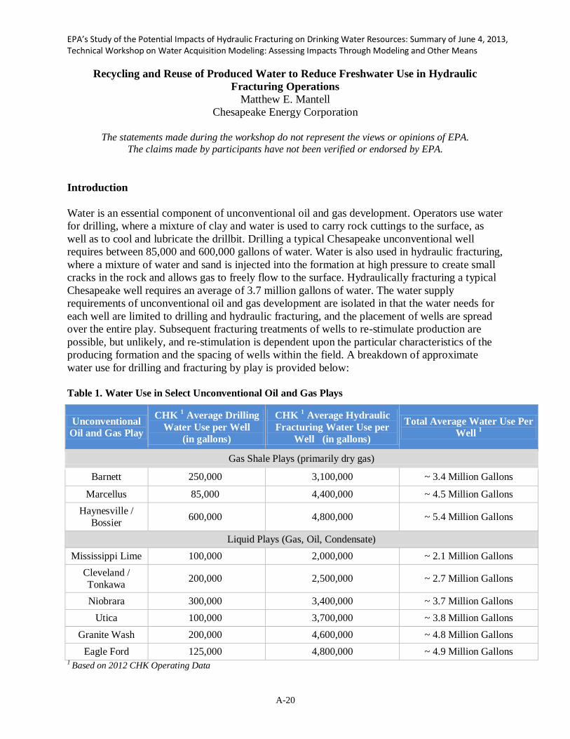
EPA’s Study of the Potential Impacts of Hydraulic Fracturing on Drinking Water Resources: Summary of June 4, 2013, Technical Workshop on Water Acquisition Modeling: Assessing Impacts Through Modeling and Other Means
A-20
Recycling and Reuse of Produced Water to Reduce Freshwater Use in Hydraulic
Fracturing Operations
Matthew E. Mantell
Chesapeake Energy Corporation
The statements made during the workshop do not represent the views or opinions of EPA.
The claims made by participants have not been verified or endorsed by EPA.
Introduction
Water is an essential component of unconventional oil and gas development. Operators use water
for drilling, where a mixture of clay and water is used to carry rock cuttings to the surface, as
well as to cool and lubricate the drillbit. Drilling a typical Chesapeake unconventional well
requires between 85,000 and 600,000 gallons of water. Water is also used in hydraulic fracturing,
where a mixture of water and sand is injected into the formation at high pressure to create small
cracks in the rock and allows gas to freely flow to the surface. Hydraulically fracturing a typical
Chesapeake well requires an average of 3.7 million gallons of water. The water supply
requirements of unconventional oil and gas development are isolated in that the water needs for
each well are limited to drilling and hydraulic fracturing, and the placement of wells are spread
over the entire play. Subsequent fracturing treatments of wells to re-stimulate production are
possible, but unlikely, and re-stimulation is dependent upon the particular characteristics of the
producing formation and the spacing of wells within the field. A breakdown of approximate
water use for drilling and fracturing by play is provided below:
Table 1. Water Use in Select Unconventional Oil and Gas Plays
Unconventional
Oil and Gas Play
CHK 1 Average Drilling
Water Use per Well
(in gallons)
CHK 1 Average Hydraulic
Fracturing Water Use per
Well (in gallons)
Total Average Water Use Per
Well 1
Gas Shale Plays (primarily dry gas)
Barnett 250,000 3,100,000 ~ 3.4 Million Gallons
Marcellus 85,000 4,400,000 ~ 4.5 Million Gallons
Haynesville /
Bossier 600,000 4,800,000 ~ 5.4 Million Gallons
Liquid Plays (Gas, Oil, Condensate)
Mississippi Lime 100,000 2,000,000 ~ 2.1 Million Gallons
Cleveland /
Tonkawa 200,000 2,500,000 ~ 2.7 Million Gallons
Niobrara 300,000 3,400,000 ~ 3.7 Million Gallons
Utica 100,000 3,700,000 ~ 3.8 Million Gallons
Granite Wash 200,000 4,600,000 ~ 4.8 Million Gallons
Eagle Ford 125,000 4,800,000 ~ 4.9 Million Gallons 1 Based on 2012 CHK Operating Data

EPA’s Study of the Potential Impacts of Hydraulic Fracturing on Drinking Water Resources: Summary of June 4, 2013, Technical Workshop on Water Acquisition Modeling: Assessing Impacts Through Modeling and Other Means
A-21
Produced Water Management
Produced water plays a key role in the environmental and economic viability of unconventional
oil and gas development. Produced water is a byproduct of all oil and natural gas (energy)
development. In order to successfully develop these resources, produced water has to be
effectively managed.
For the purposes of this discussion, produced water is all water that is returned to the surface
through a well borehole and is made up of water injected during the fracture stimulation process,
as well as natural formation water. Produced water is typically produced for the lifespan of a
well, although quantities may vary significantly by play. Produced water quality can also vary
tremendously from brackish (not fresh, but less saline than seawater) to saline (similar salinity to
seawater) to brine (which can have salinity levels multiple times higher than seawater).
Furthermore, the term flowback refers to the process of excess fluids and sand returning through
the borehole to the surface. For this discussion, the water produced during flowback operations is
considered produced water.
The feasibility of produced water reuse is dependent on three major factors. First is the quantity
of the produced water generated, including the initial volume of produced water generated
(typically during the first few weeks after stimulation). The second factor is the duration in time
of produced water generation, including the rate at which water is generated and how it declines
over time. Wells that produce significant volumes of produced water during the initial time
period are preferred for reuse due to the logistics involved in storing and transporting the water
for reuse. A continuous volume can keep tanks and trucks moving, increasing the economic
efficiency of reusing the produced water from one wellsite to another. The Mississippi Lime and
Permian Basin wells produce the highest amount of initial produced water. These plays contain
wells that produce over one million gallons of water in the first 10 days after completion. This
volume is sufficient to provide nearly 50% of the water needed to fracture a new well in these
plays. The Barnett, Eagle Ford, Granite Wash, Cleveland / Tonkawa Sand, Niobrara, Marcellus
and Utica Shale all produce a significant volume of initial produced water, enabling the
effectiveness of reuse. These plays produce between 300,000 to 1,000,000 gallons of water per
well in the first 10 days after completion (a volume sufficient to provide approximately 10% to
40% of the total water needed to fracture a new well (see Table 1 above). The Haynesville Shale
produces less water, approximately 250,000 gallons per well in the first 10 days after
completion. This is approximately 5% of the total water needed to fracture a new well, and
thereby less favorable in terms of reuse (due to logistics as mentioned above) (Chesapeake
Energy, 2012).
Long-term produced water production is also important because wells that produce large
volumes of produced water for long periods of time will require a disposal or reuse option that is
located in close proximity to the wellsite in order to retain the economic viability of the
operation. The unit of measurement used for comparison of long term produced water is gallons
of water per million cubic feet (MMCF) of gas or hydrocarbon liquid equivalent (MMCFe). This
unit of measurement for comparing volumes is exclusive to unconventional plays because there
appears to be a direct correlation between hydrocarbon production and long term produced water
generation in the major unconventional plays. Mississippi Lime and Permian Basin wells

EPA’s Study of the Potential Impacts of Hydraulic Fracturing on Drinking Water Resources: Summary of June 4, 2013, Technical Workshop on Water Acquisition Modeling: Assessing Impacts Through Modeling and Other Means
A-22
generate the largest volumes of produced water of the unconventional plays at greater than 5,000
gallons per MMCFe. Both of these plays and basins are believed to contain larger volumes of
natural formation water present in, and in close proximity to the target oil and gas development
zone. The Barnett Shale and Cleveland / Tonkawa Sand also generate relatively large amounts of
long term produced water, on the order of greater than 2,000 gallons per MMCFe. The Granite
Wash, Niobrara, Eagle Ford, and Haynesville Shale are moderate produced water generating
plays at approximately 500 to 2,000 gallons per MMCFe. These shale formations are relatively
desiccated and allow less fluid production per MMCFe. The lowest long term produced water
volumes come from the Marcellus and Utica Shales. These plays are highly desiccated
formations that tend to bind water to the shale through physical / chemical interactions. Water
production in both plays is less than 500 gallons per MMCFe with some wells producing
virtually no water with long term hydrocarbon production (Chesapeake Energy, 2012).
The third major factor in produced water reuse is the quality of the produced water. Total
dissolved solids (TDS), total suspended solids (TSS) (the larger suspended particulates in water),
scale causing compounds (calcium, magnesium, sulfate) and bacteria growth all have a major
effect on the feasibility of reusing produced water. Also, in the emerging liquids rich plays,
hydrocarbon content in the produced water also can have a major impact on the ability to treat,
store, and reuse produced water. Historically, TDS has been managed in the reuse process by
blending with freshwater to reduce the TDS. Blending was necessary because high TDS can
decrease the effectiveness of certain chemicals used for friction reduction which can be
problematic in the hydraulic fracturing process. However, new advancements in the development
of salt tolerant friction reducers by chemical suppliers have allowed operators to significantly
increase the amount of produced water reused in fracturing operations. TSS, on the other hand,
can be managed with relatively inexpensive filtration systems. Filtration of TSS is necessary
because elevated solids can cause well plugging, decrease biocide effectiveness and interfere
with other additives. Scale and bacteria causing compounds (particularly sulfates, calcium, and
magnesium) can be managed with chemical treatments or advanced filtration, but each additional
treatment step reduces the economic efficiency of the process. Hardness compounds (calcium
and magnesium) can be managed with blending, but sulfate content should be kept as low as
possible to prevent the formation of barium sulfate scale in the formation (many of the
formations contain naturally high amounts of barium). Hydrocarbons can be managed with
mechanical and chemical separation processes. It is very important to control hydrocarbon
content because it can prevent the activation of certain hydraulic fracturing additives if
hydrocarbon containing produced water is blended into a future completion (frac). The ideal
produced water for reuse has low hydrocarbon content, low TSS and little to no scale or bacteria
causing compounds.
Produced Water Treatment Options: The Chesapeake Experience
While produced water is generated with the production of oil and gas (energy) as stated above,
energy also plays a key role in determining the best way to manage produced water. Most
produced water is of relatively poor quality and may contain very high levels of natural salts and
minerals that have dissociated from the target hydrocarbon reservoir.

EPA’s Study of the Potential Impacts of Hydraulic Fracturing on Drinking Water Resources: Summary of June 4, 2013, Technical Workshop on Water Acquisition Modeling: Assessing Impacts Through Modeling and Other Means
A-23
Many different technologies are available for treatment and reuse of produced water but most
can be categorized into one of eight different treatment types. This paper will discuss the basics
of each treatment type, and will offer an operator’s perspective and experience with the
application of the technology on unconventional oil and gas produced water.
Sedimentation and Filtration: Sedimentation is simply gravity separation in a tank or
impoundment. This is the most basic of all water “treatment” processes. No chemicals or energy
are added to the water and it involves simply storing fluid for a period of time to allow the
suspended solids to “fall” out of solution. In the oilfield, this “treatment” type is only effective
for removing or settling suspended solids and if there is any type of entrainment mechanism at
work in the fluid, the solids will not properly settle out. Filtration is another simple produced
water treatment option that typically involves the use of porous media (either a “sock” or “sand”
column filter) to filter solid particles out of solution. Filtration is a great option because it is
inexpensive, the media is easy to dispose or back wash, and the systems are very easy to operate.
Most oilfield filtration systems operate on a pressure differential where sensors detect a set
pressure value (based on a clogged or dirty filter) and trigger a filter replacement or a backwash
cycle. Chesapeake Energy has utilized both sedimentation and filtration technologies extensively
in the Marcellus Shale for over 3 years. There are numerous providers offering sedimentation
and filtration “treatment systems” and the water quality in the Marcellus Shale is suitable for
these systems due to the low hydrocarbon content of the water and the low scaling tendency of
the dissolved salts that remain in solution. Chesapeake’s program in the Marcellus Shale has
been tremendously successful by reducing water disposal volumes by over 95% and is also
extremely cost effective through the reduction in transportation, water acquisition, and produced
water disposal costs. (Chesapeake Energy, 2012)
Chemical Precipitation: Chemical precipitation has a long and successful history in conventional
drinking water treatment systems. The technology utilizes chemicals and the processes of
coagulation, flocculation and sedimentation to remove contaminants from water. Coagulation
and flocculation are processes that increase the tendency of small particles in aqueous suspension
to attach to one another and accumulate in size and weight to allow for the process of gravity
settling (sedimentation) to remove the contaminants from solution (American Water Works
Association, 1999). Due to the history of the technology in municipal wastewater treatment,
many chemical precipitation providers are expanding their focus into oil and gas produced water
treatment. Typically these systems are more expensive than sedimentation and filtration options
as discussed above, but they are less expensive than the more advanced treatment options
involving membranes and thermal processes discussed below. Chesapeake Energy is currently
utilizing a chemical precipitation system (followed by filtration) to treat produced water and
drilling wastewater in the Utica Shale. The system involves chemical precipitation with a
coagulant (currently utilizing aluminum chloride) to remove suspended solids, followed by a
series of filters and the addition of a small amount of biocide to control bacteria growth in the
treatment process. All of the treated water is tested for remaining contaminants (specifically
hardness, sulfates, hydrocarbons, and TDS) and then is blended with fresh water for use in
subsequent completion operations (Chesapeake Energy, 2013).
Dissolved Air Flotation: Dissolved Air Flotation and its comparable sister technology (Induced
Gas Flotation) utilize a chemical polymer with an air or gas stream injected through a column of

EPA’s Study of the Potential Impacts of Hydraulic Fracturing on Drinking Water Resources: Summary of June 4, 2013, Technical Workshop on Water Acquisition Modeling: Assessing Impacts Through Modeling and Other Means
A-24
fluid to promote the “floating” of contaminants to the surface so they can be removed through a
skimming mechanism at the top of the column. This treatment technology is particularly
effective for produced waters with free or entrained hydrocarbons due to the fact that
hydrocarbons naturally “float” on water. This treatment technology is slightly more expensive
than most chemical precipitation options, but it is great for hydrocarbon removal and often does
not require the use of secondary filtration to remove the remaining suspended solids. As a result,
this technology has a promising future for use in the emerging oil and hydrocarbon liquid rich
unconventional plays. Chesapeake Energy is currently evaluating this technology for produced
water reuse in a number of liquid rich operating areas.
Evaporation: Evaporation is less of a produced water “treatment” technology and more of a
“waste reduction” technology. The process is very simple and uses natural processes of
evaporation to turn a portion of produced water into water vapor. Evaporation systems in the
oilfield are very energy intensive and recover no fluid or water. Due to the energy intensity of the
systems, costs can vary depending on the available energy or heat source. Many providers are
focused on using “waste heat” to drive their evaporation systems. From late 2009 to 2012
Chesapeake Energy tested and operated an evaporative reduction and solidification system in the
Barnett Shale. The utilized system was designed to run off of “waste heat” from a nearby
Chesapeake owned compressor station which was intended to reduce or eliminate the need for
the system to consume fuel. The project was successful because Chesapeake was able to
significantly reduce a large amount of produced water from being disposed of in a nearby
permitted underground injection well. However, the technology struggled to maintain the
anticipated cost effectiveness and was plagued by technical problems running off of the waste
heat from the nearby compressors (Chesapeake Energy, 2012).
Thermal Distillation: Thermal distillation is an advanced water treatment technology that targets
the removal of total dissolved solids (or salts) from produced water. The most common type of
thermal distillation method utilized in the oilfield is Mechanical Vapor Recompression (MVR).
MVR utilizes low pressure to evaporate produced water and mechanically recompresses steam to
produce the distilled water effluent. MVR systems require pretreatment with either chemical
precipitation or dissolved air flotation (as discussed above) in order to remove suspended solids
and hydrocarbons. Due to the addition of the more expensive thermal component, these systems
can be significantly higher in cost than the “pretreatment” systems (chemical precipitation and
dissolved air floatation) alone. Chesapeake Energy is currently running some long term trials
with a MVR unit in the Anadarko Basin in northwest Oklahoma and the Texas panhandle.
Chesapeake’s purpose in trialing this advanced treatment system is to help manage the risk
associated with the transport and storage of high TDS waters over long distances. Specifically,
the MVR system being utilized by Chesapeake produces three streams: one sludge waste stream
of mainly suspended solids that can be dried and landfilled, one “clean” high TDS brine waste
stream that can be transported by truck and utilized as a clay stabilizer or winterizing agent on
the next completion, and finally the distilled pure effluent stream which can be transported by
pipeline and stored in a similar method to fresh water due to the highly pure nature of the water
(Chesapeake Energy, 2013).
Electro-Coagulation: Electro-coagulation is an electrically driven treatment process that utilizes
fewer chemicals. In these systems an electric charge is passed through the fluid stream that

EPA’s Study of the Potential Impacts of Hydraulic Fracturing on Drinking Water Resources: Summary of June 4, 2013, Technical Workshop on Water Acquisition Modeling: Assessing Impacts Through Modeling and Other Means
A-25
changes the surface charge on the solid particles and causes them to agglomerate and drop out of
solution or be more efficiently filtered from solution. Electro-coagulation systems are
increasingly being offered by numerous providers, and the systems are good at removing
suspended solids and most heavy metals. The system does not treat total dissolved solids nor
does it remove hydrocarbons and it can be relatively energy intensive and does require
knowledgeable operators. Chesapeake Energy has not found a suitable application for this
technology but continues to evaluate electro-coagulation systems to see if they can compete in
terms of economics and performance versus other treatment systems.
Crystallization: Crystallization is the most comprehensive and advanced treatment technology
available for produced water on the market today. Crystallizers are utilized to completely remove
all dissolved solids (including all salts) from solution and can achieve a zero liquid waste
discharge (only solid salt and distilled water outputs). Crystallizers do require pretreatment (via
chemical precipitation, dissolved air floatation, or membrane filtration), followed by distillation,
before the crystallization step is applied. Due to the advanced and comprehensive nature of the
treatment system, and the thermal energy input required to run the system, this is the most
expensive treatment option available, but as mentioned, it does eliminate the need for liquid
disposal. Chesapeake Energy has been in discussions with a number of vendors about the
possibility of utilizing a crystallizer at some point in the future in the Marcellus Shale, but at this
time Chesapeake has no current or planned use.
Reverse Osmosis Membranes: Reverse Osmosis (RO) membrane filtration is the preferred
treatment technology for seawater desalination and the technology has naturally migrated over
for consideration in the oilfield. Due to the nature of the technology, RO systems require a very
steady water quality and a comprehensive pretreatment system to ensure suspended solids and
hydrocarbons do not impact the membrane as they can immediately foul or ruin most RO
membranes. RO systems are also very prone to scaling without comprehensive pretreatment and
output efficiency begins to decline sharply for TDS levels above that of seawater. Due to the
high salinity and variability in water quality of most unconventional produced water brines, RO
has limited potential in most unconventional plays. For reference, most unconventional produced
water TDS levels can easily reach 2-5 times the TDS content in typical seawater. Due to these
hurdles, Chesapeake Energy has not found a suitable application for the technology, but as new
advancements in scale and hydrocarbon resistant coatings and robust membrane materials
advance, potential applications could emerge in the future (Chesapeake Energy, 2013).
Despite the numerous classifications and types of treatment technologies described above, all
treatment processes have energy, environmental and economic impacts that are directly impacted
by produced water quality. Simple conventional water treatment processes (coagulation,
flocculation, sedimentation, and filtration) do require energy, but are typically much less energy
intensive than advanced salt separation treatment processes (reverse osmosis membranes,
thermal distillation systems, and crystallization systems). Furthermore, some of the water
treatment processes such as coagulation and flocculation, dissolved air floatation, distillation,
and crystallization require chemicals (sometimes in large volumes) which also have energy,
environmental and economic related impacts.

EPA’s Study of the Potential Impacts of Hydraulic Fracturing on Drinking Water Resources: Summary of June 4, 2013, Technical Workshop on Water Acquisition Modeling: Assessing Impacts Through Modeling and Other Means
A-26
Advancements in Hydraulic Fracturing Chemistries Reduce Need for Fresh Water
Chesapeake Energy has been very involved with a number of hydraulic fracturing chemical
suppliers in getting salt or “brine” tolerant chemicals developed in an effort to increase the use of
produced water in fracturing operations. One area of tremendous success has been the industry
development of salt tolerant friction reducers. Friction reducers are polymers that are the primary
component of “slickwater” fracturing fluid systems. In the past, high TDS produced waters
would prevent the fresh water-based friction reducers from working properly. With the
advancements in chemistry, these new friction reducers have allowed Chesapeake Energy to
substantially increase the percentage of high TDS brine utilized in hydraulic fracturing
operations. Specifically, in the Mississippi Lime play in northwest Oklahoma, Chesapeake has
completed over three dozen wells using 100% high TDS (over 200,000 ppm TDS) produced
water. A recent evaluation of the trial program has shown no detrimental impact to production
utilizing the high TDS produced water and the program has yielded some substantial economic
benefits (particularly the reduction in produced water sent to disposal). The one water quality
criteria that must be managed very carefully in these direct reuse applications is the presence of
hydrocarbons in the produced water which can interfere with friction reducer performance. Also,
the new salt tolerant chemistries are more expensive than their fresh water counterparts, an
important consideration to keep in mind. Chesapeake Energy is continuing to work with
chemical suppliers to develop other salt tolerant hydraulic fracturing products including gelling
agents and cross linkers (which can be particularly susceptible to some dissolved solids)
(Chesapeake Energy, 2013).
Other Considerations
Outside of treatment for reuse, disposal, via permitted, Class II UIC wells, is the long standing
and safe, produced water management option. Outside of the Marcellus Shale, salt water disposal
wells (SWDs) are by far the most common method of disposing of produced fluids from
unconventional oilfield operations. Surface discharge via wastewater treatment plants has
historically been a common treatment technique in the northeast United States, but has been
phased out due to strict discharge regulations and natural evolution of the industry due to the
Marcellus Shale development. As a note, Chesapeake Energy does not currently discharge any
produced water either directly, or via wastewater treatment plants in any operating area.
Conclusions
Energy, environmental and economic considerations must be carefully considered when
discussing possible reuse and disposal options for produced water. Much discussion and
technology development has focused on treatment technologies that can treat produced water so
it is suitable for some form of reuse. These options include reuse in oil and gas operations,
municipal, agricultural, and/or industrial operations. Lower dissolved solids produced water (<
30,000 ppm TDS) may be feasible for treatment to reuse outside of oil and gas operations.
Higher dissolved solid produced waters (> 30,000 ppm TDS) should only be reused where the
high salt/salinity content can be kept in solution (to avoid the intense energy input to separate

EPA’s Study of the Potential Impacts of Hydraulic Fracturing on Drinking Water Resources: Summary of June 4, 2013, Technical Workshop on Water Acquisition Modeling: Assessing Impacts Through Modeling and Other Means
A-27
salts). Operators have successfully demonstrated this ability by using conventional treatment
processes on high TDS waters and managing the TDS by blending the fluids in hydraulic
fracturing operations, or by utilizing new salt tolerant hydraulic fracturing additives. The
feasibility of relying on high TDS produced waters for potential municipal or agricultural water
supply does not make sense from an energy, economic or environmental perspective due to the
availability of alternative low quality water resources that could be treated to acceptable
standards with far lower energy inputs. This includes municipal wastewater, brackish
groundwater, and even seawater when logistically feasible. Based on this same logic,
environmental and economic benefits may directly correlate when evaluating reuse versus
disposal. For example, in areas with extensive salt water disposal well infrastructure like the
Barnett Shale or Mississippi Lime, salt water disposal wells are in close proximity to operations,
and are a low cost, low energy, safe and effective alternative to advanced reuse. The energy
requirements needed to treat Barnett Shale or Mississippi Lime produced water (outside of direct
filtration and blending) is significant. Since all energy sources result in some form of air
emissions, water use, and/or waste generation; reusing produced water in these plays using an
advanced treatment technology may have greater negative environmental impacts than salt water
disposal. Furthermore, oil and gas operations that keep dissolved solids in solution and use the
fluid in completion operations for subsequent wells can effectively reduce the volume of fresh
water needed for future operations by significant amounts. The onshore unconventional oil and
gas industry has recently been very successful in utilizing conventional, low energy treatment
systems to remove suspended solids, metals, and hydrocarbons from produced water and then
reusing this water in hydraulic fracturing operations. From an energy efficiency standpoint, this
is a much more efficient use of energy and water than treating produced water to drinking water
standards.

EPA’s Study of the Potential Impacts of Hydraulic Fracturing on Drinking Water Resources: Summary of June 4, 2013, Technical Workshop on Water Acquisition Modeling: Assessing Impacts Through Modeling and Other Means
A-28
APPENDIX A: Removal of Water from the Effective Hydrologic Cycle: Concerns Put to
Rest
One of the major criticisms to the use of water in the development of oil and natural gas supplies,
particularly in the hydraulic fracturing of unconventional oil and gas plays, is the so-called
“permanent removal” of water from the surface and near sub-surface hydrologic cycle referred to
in this paper as the effective hydrologic cycle. While the focus of this paper is recycling and reuse
of produced water to reduce fresh water use in hydraulic fracturing operations, it is important to
address this “permanent removal” from the effective hydrologic cycle criticism.
Like all energy development, all oil and natural gas development activities use water resources.
In unconventional oil and gas development, water is used specifically for drilling and hydraulic
fracturing. As discussed earlier, the majority of water is used in the hydraulic fracturing process.
Water demands for hydraulic fracturing and the volumes of produced water generated can vary
significantly between plays. Highly desiccated, water loving formations like the Marcellus and
Utica Shales trap and bind a majority of the water used in the hydraulic fracturing process to the
formation. As a result, these wells, over their productive lifetime, will generate only a fraction of
the produced water used during the fracturing process. Higher water bearing plays or plays near
water bearing formations like the Mississippi Lime and Barnett Shale generate much higher
volumes of produced water. These wells over their lifespan will generate many times the original
volume used in the fracturing process. However, regardless of how much produced water is
generated, the safest and highly preferred disposal method for produced water is underground
injection via permitted Class II SWDs. (Chesapeake Energy, 2012)
Regardless of the unconventional play, since the majority of produced water either remains in the
formation or is disposed of in another suitable geologic formation (via Class II SWDs), this
water is indeed removed from the effective hydrologic cycle. This may lead some to criticize and
treat oil and natural gas water use differently than other major water users like power plants who
consume water during the cooling process. The argument is the power plant type of consumption
is evaporation and the volume of water evaporated is simply released to the atmosphere as water
vapor and is still in the effective hydrologic cycle.
These concerns about the permanent loss of water from the effective hydrologic cycle via drilling
and hydraulic fracturing can easily be addressed with a simple explanation of natural gas
combustion (and a slightly more complicated variation can explain liquid hydrocarbon
combustion). When natural gas is combusted with oxygen (air) it forms two by-products, carbon
dioxide and water vapor. The balanced combustion reaction is shown below:
CH4 + 2O2 CO2 + 2H2O
It is the generation of water vapor that ultimately offsets the removal of water from the effective
hydrologic cycle. Based on some common assumptions about natural gas and natural gas
combustion, approximately 10,675 gallons of water vapor are produced with the combustion of
one MMCF of natural gas. (These calculations are shown in detail along with all assumptions in
Appendix below.) This volume of water vapor generation was applied to determine
approximately how much natural gas needs to be generated and combusted to offset the volume
of water used in the development of a typical dry gas well in each of the major shale gas plays.

EPA’s Study of the Potential Impacts of Hydraulic Fracturing on Drinking Water Resources: Summary of June 4, 2013, Technical Workshop on Water Acquisition Modeling: Assessing Impacts Through Modeling and Other Means
A-29
The results are calculated and shown in Table 2 including the average amount of time needed for
a typical Chesapeake well to produce the volume of natural gas needed to offset the water used
in the well.
Table 2: Water Vapor Combustion and Effective Hydrologic Cycle Volume Recovery by Major
Shale Gas Play
Shale Play
Average
Water Use
Per Well
(in gallons)*
CHK Estimated
Average Natural
Gas Production
Over the Life of
Well
(in cubic feet) **
Cubic Feet of Natural Gas
Needed for Combustion to
Offset Shale Gas Water
Use (Based on 10,675
gal/MMCF Natural Gas
Combusted)
Time for an
Average CHK
Well to Produce
Needed Natural
Gas to Offset
Water Used in
Well
Haynesville 5,400,000 6,500,000,000 505,000,000 < 6 Months
Marcellus 4,500,000 5,750,000,000 421,000,000 < 6 Months
Barnett 3,400,000 3,300,000,000 320,000,000 < 6 Months
Source: *Chesapeake 2012, **Chesapeake 2012a
As shown above, a well in any of the three major shale gas plays produces enough natural gas in
less than six months, that when combusted, offsets the entire volume of water used in the
development of that well. Keep in mind these wells are anticipated to produce natural gas for
more than 20 years (Chesapeake Energy, 2012).

EPA’s Study of the Potential Impacts of Hydraulic Fracturing on Drinking Water Resources: Summary of June 4, 2013, Technical Workshop on Water Acquisition Modeling: Assessing Impacts Through Modeling and Other Means
A-30
Water Vapor from the Combustion of Natural Gas Calculations
Assumptions:
Typical natural gas makeup assumptions:
Methane (CH4) ~ 95%
Ethane (C2H6) Propane (C3H8) n-Butane (C4H10) ~5% combined Carbon Dioxide (CO2) Nitrogen (N) Sulfur (S)
Due to variations in natural gas makeup (above), the conservative approach was to only use methane to calculate water vapor production, although ethane (C2H6), propane (C3H8) and n-
butane (C4H10) when combusted will also produce water vapor.
Balanced Equation for Methane Combustion: CH4 + 2O2 CO2 + 2H2O
Assume normal temperature and pressure (68oF and 1atm)
Volume of 1 mole of CH4 at 68oF is 0.0026 lb mole/ft
3
Molecular weight of water is 18 lb/lb mole
Liquid water density at 68oF is 8.33 lbs/gallon
Calculations:
Step One: Determine how much methane is in one million cubic feet (MMCF) of natural gas:
1. 1,000,000 cu-ft of natural gas x 0.95 (methane component) = 950,000 cu-ft of CH4
Step Two: Determine the number of pound mol of CH4 using the assumption above for the volume of one
mole of CH4.
2. 950,000 cu-ft of CH4 x (0.0026 lb mol CH4 / ft3 of CH4) = 2,470 lb mol CH4
Step Three: Using the balanced equation above, determine how many pounds of mols of water vapor are
produced in the combustion process.
3. 2,470 lb mol CH4 x (2 lb mol H2O / 1 lb mol CH4) = 4,940 lb mol H2O
Step Four: Using the molecular weight of water, determine how many pounds of water vapor are
produced in the combustion process.
4. 4,940 lb mol H2O x (18 lb H2O/1 lb mol H2O) = 88,920 lb H2O
Step Five: Using the liquid water density, determine the volume of water vapor produced. 5. 88,920 lb H2O x (1 gal H2O/8.33 lb H2O) = 10,675 gals H2O (as vapor) per MMCF
Note: Not all natural gas that is consumed is combusted. According to a 1995 DOE Topical Report on “Economic Evaluation and Market Analysis for Natural Gas Utilization,” approximately 3.5% (relatively
negligible) of natural gas is used as feedstock for ammonia, methanol, ethylene and hydrogen production.

EPA’s Study of the Potential Impacts of Hydraulic Fracturing on Drinking Water Resources: Summary of June 4, 2013, Technical Workshop on Water Acquisition Modeling: Assessing Impacts Through Modeling and Other Means
A-31
References
Chesapeake Energy, operational experience, 2012.
American Water Works Association (1999) Water Quality and Treatment: A Handbook of Community Water Supplies. 6.1-6.2.
Chesapeake Energy, operational experience, 2013.
Chesapeake Energy, corporate data, 2012a.

EPA’s Study of the Potential Impacts of Hydraulic Fracturing on Drinking Water Resources: Summary of June 4, 2013, Technical Workshop on Water Acquisition Modeling: Assessing Impacts Through Modeling and Other Means
B-1
Appendix B.
Extended Abstracts from Session 2: Current and Future Trends in Hydraulic Fracturing Wastewater
Management

EPA’s Study of the Potential Impacts of Hydraulic Fracturing on Drinking Water Resources: Summary of June 4, 2013, Technical Workshop on Water Acquisition Modeling: Assessing Impacts Through Modeling and Other Means
B-2
Evaluating Scenarios of Potential Impact of Water Acquisition for Hydraulic Fracturing
Stephen R. Kraemer
U.S. Environmental Protection Agency, Office of Research and Development
Information presented in this abstract is part of the EPA’s ongoing study. EPA intends to use
this, combined with other information, to inform its assessment of the potential impacts to drinking water resources from hydraulic fracturing. Mention of trade names or commercial
products does not constitute endorsement or recommendation for use.
The US EPA Hydraulic Fracturing (HF) study is evaluating the question “How might water
withdrawals affect short- and long-term water availability in an area with hydraulic fracturing
activity?” The project described here is using computer simulations to evaluate future scenarios
of water withdrawals supporting HF and the potential impact on water resources available for
drinking water use. The background and progress of this project is contained in Study of the
Potential Impacts of Hydraulic Fracturing on Drinking Water Resources: Progress Report (US
EPA, 2012). The Quality Assurance Project Plan (QAPP) outlines the approach for the basin
scale assessment (Cadmus, 2012).
An outline of the project critical path for modeling impact is shown in Figure 1.
Figure 7. Watershed modeling critical paths, from setup to calibration/validation to scenario runs
starting with the foundational baseline/historical, updating to baseline/current, culminating in the
evaluation of the futures (business-as-usual, energy plus, and recycling plus).
The EPA recognizes the unique circumstances of the geography and geology of every
unconventional oil and gas resource and has chosen two study sites to initially explore and
identify the potential differences related to water acquisition. The study areas include: the
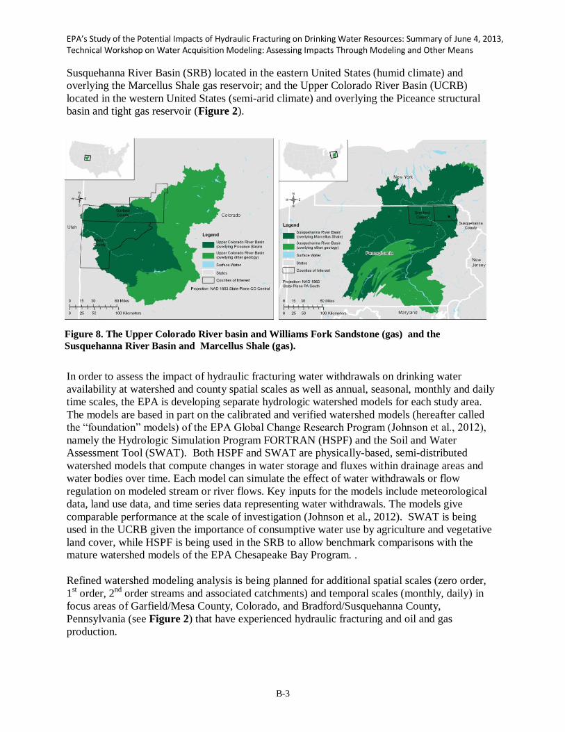
EPA’s Study of the Potential Impacts of Hydraulic Fracturing on Drinking Water Resources: Summary of June 4, 2013, Technical Workshop on Water Acquisition Modeling: Assessing Impacts Through Modeling and Other Means
B-3
Susquehanna River Basin (SRB) located in the eastern United States (humid climate) and
overlying the Marcellus Shale gas reservoir; and the Upper Colorado River Basin (UCRB)
located in the western United States (semi-arid climate) and overlying the Piceance structural
basin and tight gas reservoir (Figure 2).
In order to assess the impact of hydraulic fracturing water withdrawals on drinking water
availability at watershed and county spatial scales as well as annual, seasonal, monthly and daily
time scales, the EPA is developing separate hydrologic watershed models for each study area.
The models are based in part on the calibrated and verified watershed models (hereafter called
the “foundation” models) of the EPA Global Change Research Program (Johnson et al., 2012),
namely the Hydrologic Simulation Program FORTRAN (HSPF) and the Soil and Water
Assessment Tool (SWAT). Both HSPF and SWAT are physically-based, semi-distributed
watershed models that compute changes in water storage and fluxes within drainage areas and
water bodies over time. Each model can simulate the effect of water withdrawals or flow
regulation on modeled stream or river flows. Key inputs for the models include meteorological
data, land use data, and time series data representing water withdrawals. The models give
comparable performance at the scale of investigation (Johnson et al., 2012). SWAT is being
used in the UCRB given the importance of consumptive water use by agriculture and vegetative
land cover, while HSPF is being used in the SRB to allow benchmark comparisons with the
mature watershed models of the EPA Chesapeake Bay Program. .
Refined watershed modeling analysis is being planned for additional spatial scales (zero order,
1st order, 2
nd order streams and associated catchments) and temporal scales (monthly, daily) in
focus areas of Garfield/Mesa County, Colorado, and Bradford/Susquehanna County,
Pennsylvania (see Figure 2) that have experienced hydraulic fracturing and oil and gas
production.
Figure 8. The Upper Colorado River basin and Williams Fork Sandstone (gas) and the
Susquehanna River Basin and Marcellus Shale (gas).

EPA’s Study of the Potential Impacts of Hydraulic Fracturing on Drinking Water Resources: Summary of June 4, 2013, Technical Workshop on Water Acquisition Modeling: Assessing Impacts Through Modeling and Other Means
B-4
Acknowledgements
This work was supported by EPA Contract EP-C-08-002, Task Order 32 (Stephen Kraemer, EPA
WAM) to The Cadmus Group, Inc.(Laura Blake, Project Manager, Jonathan Koplos, Andy
Somor, Corey Godfrey) in conjunction with subcontractors AQUA TERRA Consultants (Paul
Duda, John Imhoff, Tony Donigian) and Texas A&M University (Debjani Deb, Raghavan
Srinivasan). We also acknowledge the contributions in the area of data collection by Shaw
Environmental Consultants (Johnathan Shireman) under EPA Contract EP-C-08-034, Work
Assignment HF-2-10 (Susan Mravik, EPA WAM). Jim Kitchens is the project Quality
Assurance Manager. Refinement modeling work continues with the assistance of Yusuf
Mohamoud, Chris Knightes, Mark Gabriel, Lourdes Prieto, and Keewook Kim, John Johnston,
Kate Sullivan, and Roy Sidle of the EPA ORD laboratory in Athens, Georgia.
References
Cadmus Group, Inc, 2012. Quality Assurance Project Plan: Modeling the Impact of Hydraulic
Fracturing (HF) on Water Resources Based on Water Acquisition Scenarios, Prepared by
the Cadmus Group, Inc., in conjunction with subcontractors AQUA TERRA Consultants
and Texas A&M University, (revised September 4, 2012).
http://www2.epa.gov/hfstudy/quality-assurance-project-plan-modeling-impact-hydraulic-
fracturing-water-resources-based-0
Johnson, T.E., J.B. Butcher, A. Parker, and C.P. Weaver, 2012. Investigating the Sensitivity of
the U.S. Streamflow and Water Quality to Climate Change: U.S. EPA Global Change
Research Program’s 20 Watersheds Project, Journal of Water Resources Planning and
Management, ASCE, 138:453-464.
US EPA, 2012. Study of the Potential Impacts of Hydraulic Fracturing on Drinking Water
Resources: Progress Report, EPA 601/R-12/011 (December 2012). www.epa.gov/hfstudy

EPA’s Study of the Potential Impacts of Hydraulic Fracturing on Drinking Water Resources: Summary of June 4, 2013, Technical Workshop on Water Acquisition Modeling: Assessing Impacts Through Modeling and Other Means
B-6
Mapping Water Availability and Cost in the Western United States Vincent C. Tidwell,
1 Barbara D. Moreland,
1 Katie M. Zemlick,
1 Barry L. Roberts,
1 Howard Passell
1
Daniel Jensen,2 Christopher Forsgren,
2 Gerald Sehlke
3
Margaret Cook,4 Carey King,
4 and Sara Larsen
5
1Sandia National Laboratories 2Idaho National Laboratory
3University of Idaho
4University of Texas
5Western States Water Council
The statements made during the workshop do not represent the views or opinions of EPA.
The claims made by participants have not been verified or endorsed by EPA.
Introduction
Concern over the availability of water to meet future energy sector demands has been expressed
(GAO 2013; DOE 2006). In 2011 the Department of Energy’s Office of Electricity initiated a
project with the Western Electricity Coordinating Council (WECC) and the Electric Reliability
Council of Texas (ERCOT) to investigate potential impacts of limited water availability on long
term transmission planning. Technical support for the effort is led by Sandia National
Laboratories with the supported of Argonne National Laboratory, Idaho National Laboratory, the
National Renewable Energy Laboratory, Pacific Northwest National Laboratory, the University
of Texas, and the Electric Power Research Institute.
As a basis for transmission planning, water availability, cost, and projected future demand are
mapped for the 17-conterminous states in the western U.S. Specifically, water availability is
mapped according to five unique sources including unappropriated surface water, unappropriated
groundwater, appropriated surface/groundwater, municipal waste water, and brackish
groundwater. Associated costs to acquire, convey and treat the water, as necessary, for each of
the five sources are also estimated. To complete the picture, competition for the available water
supply is projected over the next 20 years.
Methods
Raw data were acquired from a variety of sources. Where available, data were collected directly
from the western states. In collecting the data we worked directly with state water data experts to
identify and at times gain access to the data. In most cases the data came from the state’s water
plan that was generally available from on-line sources. Efforts were made to vet the collected
water data with the state experts to verify the fidelity of data collected and any data
conversion/translation made to render the data in a consistent and comparable format. Federally
reported data were used as necessary to fill in gaps, including information derived from the U.S.
Geological Survey, Environmental Protection Agency, Energy Information Administration, U.S.
Department of Agriculture and others.
This analysis makes use of multiple data sets from multiple sources reported at differing
geographic resolutions (e.g., point, county, watershed, state). For purposes of this analysis, a

EPA’s Study of the Potential Impacts of Hydraulic Fracturing on Drinking Water Resources: Summary of June 4, 2013, Technical Workshop on Water Acquisition Modeling: Assessing Impacts Through Modeling and Other Means
B-7
consistent reference system is required. The 8-digit Hydrologic Unit Code (HUC) watershed
classification (e.g., Seaber et al. 1987) is adopted, which resolves the 17 western states into1208
unique hydrologic units. The 8-digit HUC is selected as it provides a physically meaningful unit
relative to water supply/use and provides the highest level of detail that can be justified with the
data consistently available across all 17 western states. For raw data reported in point-format,
translation to the 8-digit HUC is achieved by simple aggregation/averaging. For raw data
reported in polygonal-format, translation follows a simple population or areal weighting. In the
case of water use data, the 1995 USGS water use reported at the 8-digit level (Solley et al. 1995)
provides the needed spatial weighting function.
There are no definitive measures of water availability and cost that entirely span the full 17-state
region. Rather, these metrics must be developed from the raw data collected from the states and
federal agencies. The challenge is to formulate water availability and cost metrics that
appropriately balance the underlying complexity of the system (e.g., physical hydrology, climate,
use characteristics, technology and water management institutions) with the data that is
consistently available across the entire western U.S. To assist in striking such a balance, water
availability/cost metrics are formulated with the help of subject experts. Specifically,
representatives from the Western Governors’ Association, Western States Water Council, USGS,
and individual state water management agencies assisted in defining appropriate and informative
water metrics (in total the team included 11 participants plus the author team). These metrics
were developed and vetted over a two month period during 6 webinars lasting roughly 90
minutes each. The resulting metrics are described below.
Water Availability Metrics
Unappropriated Surface Water
States exercise full authority in matters pertaining to off-stream water use. In the western states
water is managed according to the doctrine of prior appropriation, which defines a system of
priority where the first to make beneficial use of water has the first right to it in times of drought.
Access to this water requires only a permit or water right issued by the state’s water management
agency. However, any new water development is allocated the most junior priority in the basin,
thus delivery in times of drought may be limited. Whether water is available for new
development depends on characteristics of the physical water supply, the water rights structure in
relation to supply, and related instate compacts and international treaties. Additionally,
navigational or environmental regulation may further limit allocation or timing of deliveries.
Particularly in arid regions the states have estimated how much surface water is available for
new development. Although the states have different terms for such water, we refer to it as
unappropriated surface water.
For purposes of this analysis, state estimated unappropriated surface water values are adopted
where available, including Arizona, Colorado, Nevada, New Mexico, Oklahoma, Oregon, Texas,
Utah, and Wyoming. Estimates of available unappropriated surface water are based on years
with normal stream flow. Although availabilities based on drought flows would yield a more
dependable estimate for new development, such estimates were available only for a single state,
Texas. For states that have not estimated unappropriated surface water availability, efforts are
made to first identify basins closed to new appropriation, in such cases available unappropriated

EPA’s Study of the Potential Impacts of Hydraulic Fracturing on Drinking Water Resources: Summary of June 4, 2013, Technical Workshop on Water Acquisition Modeling: Assessing Impacts Through Modeling and Other Means
B-8
water is set equal to zero. In the remaining open basins, streams tend to lack regulation by
interstate compacts and flows tend to be large with respect to water use. Given this lack of
stringent control on water use, environmental concerns are the most likely factor to constrain
new water development. A widely used environmental standard in the U.S. (Reiser et al. 1989) is
based on studies by Tennant (1976) which found streams maintain excellent to good ecosystem
function when stream flows are maintained at levels of ≥60-30% of the annual average. For this
study we adopt a conservative threshold of 50% to define unappropriated surface water. Thus for
basins where estimates are not available directly from the states, unappropriated surface water is
calculated as:
where j designates the watershed, Qavg is the long term annual average gauged stream flow, C is
the total consumptive use of water upstream of the gauging point. Annual average stream flow
data are taken from the National Hydrography Dataset (NHDPlus 2005) while consumptive
water use data are taken directly from individual state estimates.
Unappropriated Groundwater
States exercise full authority over the allocation of groundwater resources. Determining the
availability of groundwater for future development is complicated by numerous factors including
the manner with which groundwater is managed (e.g., strict prior appropriation, right of capture);
the physical hydrology of the basin; degree of conjunctive management between surface and
groundwater resources; allowable depletions, and a variety of other issues. Except in very limited
cases, the states have not broadly estimated and published data on the availability of
unappropriated groundwater.
Given the aforementioned complexity and relative lack of supporting data, a simple water
balance approach is adopted to identify potable groundwater that is potentially available for
development. That is, unappropriated groundwater is set equal to the difference between annual
average recharge and annual groundwater pumping. Recharge rates are taken from U.S.
Geological Survey (2003), which are derived from stream baseflow statistics, while pumping
rates are taken from state data where available or from U.S. Geological Survey (Kenny et al.
2009) otherwise.
To account for unique groundwater management and/or aquifer characteristics, further
restrictions on unappropriated groundwater availability are introduced. Specifically, availability
is set to zero in watersheds located within state defined groundwater protection zones (data
acquired directly from each state). Groundwater availability is likewise set to zero in watersheds
realizing significant groundwater depletions (historical groundwater declines exceeding 40 ft. as
given by Reilly and others [2008]). Finally, groundwater availability is set equal to zero in any
watershed that 10% or less of its land area is underlain by a principle aquifer (Reilly et al. 2008).
Appropriated Water
This source attempts to quantify water that could be made available for new development by
abandonment and transfer of the water right from its prior use. Such transfers have traditionally
involved sales of water rights off irrigated farm land to urban uses. The potential for such
transfers is estimated based on the irrigated acreage in a given watershed that is devoted to low

EPA’s Study of the Potential Impacts of Hydraulic Fracturing on Drinking Water Resources: Summary of June 4, 2013, Technical Workshop on Water Acquisition Modeling: Assessing Impacts Through Modeling and Other Means
B-9
value agricultural production; specifically, irrigated hay and alfalfa. Data (irrigated acreage and
water volume applied) are taken from the U.S. Department of Agriculture’s Agricultural Census
(USDA 2007). There is often resistance to large areas of irrigated agriculture being abandoned.
As such, land abandonment is limited to 5% of the total irrigated acreage in the watershed. This
limit is based on the state projected average decline in irrigation across the western U.S.
For watersheds experiencing significant groundwater depletions (see unappropriated
groundwater metric above) the available appropriated water is reduced by 50%. This is to
account for the fact that some portion of future water rights abandonment is likely to be used to
offset the groundwater depletion (Brown 1999).
Municipal Waste Water
Non-fresh water supplies offer important opportunities for new development. Municipal waste
water is rapidly being considered as an alternative source of water for new development,
particularly in arid regions. Municipal waste water discharge data is relatively consistently
available throughout the U.S. The Environmental Protection Agency publishes a pair of
databases (Permit Compliance System [EPA 2011], and Clean Watershed Needs Survey [EPA
2008]) that provide information on the location, discharge, and level of treatment for most waste
water treatment plants in the U.S. Additionally, the U.S. Geological Survey (Kenny et al. 2009)
publishes municipal waste water discharge values aggregated at the county level. These three
sources of information are combined to provide a comprehensive view of current waste water
discharge across the West. Lastly, the projected growth in municipal waste water discharge to
2030 is estimated (see future Water Demand section below) and added to the current discharge
rates.
However, not all of this discharge is available for future use. A considerable fraction of waste
water discharge is currently re-used by industry, agriculture, and thermoelectric generation. Re-
use estimates are determined both from the U.S. Geological Survey (Kenny et al. 2009) data as
well as the Environmental Protection Agency databases (as they record the point of discharge,
e.g., stream, agriculture, power plant and in some cases are designated as discharging to ‘reuse’).
These re-use estimates are subtracted from the projected discharge values.
In western states the availability of municipal waste water must consider return flow credits.
Those municipalities that discharge to perennial streams receive return flow credits for treated
waste water. This water is not available for new development as it is already being put to use
downstream. Unfortunately, there are no comprehensive data on waste water return flow credits.
In efforts to identify plants that are likely credited for their return flows, those plants that directly
discharge to a perennial stream are identified (point of discharge is identified in the databases
noted above). These plants are excluded as a source of available municipal waste water.
Shallow Brackish Groundwater
For this analysis brackish water availability is limited to resources no deeper than 2500 feet and
salinities below 10,000 total dissolved solids (TDS). Deeper, more concentrated resources would
generally be very expensive to exploit.
Estimates of brackish groundwater resources across the western U.S. are very spotty. To cover
this entire area requires the use of multiple sources of information. The best quality data are state

EPA’s Study of the Potential Impacts of Hydraulic Fracturing on Drinking Water Resources: Summary of June 4, 2013, Technical Workshop on Water Acquisition Modeling: Assessing Impacts Through Modeling and Other Means
B-10
estimated volumes of brackish groundwater that are potentially developable; however, this data
is only available for Texas (LBG-Guyton Associates 2003), New Mexico (Huff 2004), and
Arizona (McGavock 2009). States limit exploitation of the resource by applying some type of
allowable depletion rule. In this case it is assumed that only 25% of the resource can be depleted
over a 100 year period of time (annual available water is determined by multiplying estimated
total volume of brackish water by 0.0025).
The next best source of data is reported use of brackish groundwater as published by the U.S.
Geological Survey (Kenny et al. 2009). This does not provide a direct measure of available
water, simply an indication that brackish water of developable quality is present. Conservatively
we assume that double the existing use could be developed up to a maximum limit of 8.4X10⁻²
acre-feet per year (AF/yr). Also assumed is that the minimum quantity available is 8.4X10⁻³
AF/yr.
Finally, if a watershed has no brackish water volume estimate or brackish water use then the
presence of brackish groundwater wells is used. The U.S. Geological Survey maintains the
National Water Information System (NWIS) database which contains both historical and real-
time data of groundwater well depth and quality (USGS 2011). Where at least one well exists
brackish water availability is set to 8.4X10⁻³
AF/yr. To avoid brackish water that is in
communication with potable stream flow, availability is set to zero when the average depth to
brackish water is less than 50 ft. and the salinity is less than 3000 TDS.
Water Cost Metrics
Each of the five sources of water carry a very different cost associated with utilizing that
particular supply. The interest here is to establish a consistent and comparable measure of cost to
deliver water of potable quality to the point of use. As with water availability, costs are resolved
at the 8-digit HUC level. Considered are both capital and operating and maintenance (O&M)
costs. Capital costs capture the purchase of water rights as well as the construction of
groundwater wells, conveyance pipelines, and water treatment facilities, as necessary. All capital
costs are amortized over a 30-yr horizon and assume a discount rate of 6%. O&M costs include
expendables (e.g., chemicals, membranes), labor, waste disposal as well as the energy to lift,
move and treat the water. Below, specifics unique to each source are discussed.
Unappropriated Surface Water
No costs are assigned to unappropriated surface water. It is recognized that there are costs
associated with constructing intake structures and permitting. Such costs are not considered in
part because of the wide range of variability across use types and location. More importantly,
similar intake and permitting costs will be realized with all five sources of water, thus estimating
these uncertain costs are of little value to this effort.
Unappropriated Groundwater
Estimated costs consider both capital and O&M costs to lift water for use. Capital costs for
drilling are estimated along with electricity to lift water following the approach outlined in
Watson and others (2003). Depth to groundwater is taken from U.S. Geological Survey well log
data (USGS 2011) and averaged at the 8-digit HUC level.

EPA’s Study of the Potential Impacts of Hydraulic Fracturing on Drinking Water Resources: Summary of June 4, 2013, Technical Workshop on Water Acquisition Modeling: Assessing Impacts Through Modeling and Other Means
B-11
Appropriated Surface Water
Water rights transfer costs are based on historic data collected by the Water Strategist and its
predecessor the Water Intelligence Monthly (Water Strategist 2012). Costs are estimated by state
because of the limited availability of data. Only transactions involving permanent transfers from
agriculture to urban/industrial use are considered. Recorded transfers are averaged by year and
by state and the average of the last 5 years used for purposes of this study. No efforts are made to
project how costs may vary in time given the wide range of factors and associated uncertainty
that plays into the water transfers market.
Municipal Waste Water
Estimated costs consider expenses to lease the waste water from the municipality, convey the
water to the new point of use, and to treat the waste water. Fees charged to lease treated waste
water from the municipality were estimated based on the initial work of the Electric Power
Research Institute (EPRI 2008). Values reported in the EPRI report were verified and updated as
necessary based on a review of fees published on line. As no geospatial or plant related trends
were noted in the pricing an average of the reported fees was adopted for this study, which was
calculated at $1.21 per thousand gallons.
Conveyance of treated waste water from the treatment plant to the point of use is a potentially
important cost. Considered are both capital construction costs for a pipeline and O&M costs
principally related to electricity for pumping. Associated costs calculations are consistent with
Watson and others (2003). The key factor in this analysis is the distance between the treatment
plant and point of use. Distance values are calculated as a function of the land use density around
the existing treatment plant. Land use densities were calculated within a 5 mile buffer around all
existing treatment plants with conveyance distances simply distributed according to a rank order
of land density with low values given a conveyance distance of 1 mile to the highest land use
density given a distance of 5 miles.
It is assumed that all waste water must be treated to advanced standards before it can be re-used.
This conservative assumption was adopted considering both realized improvements in
downstream operations (e.g., increased cycles of use, reduced scaling, improved feed quality)
and the current trend of regulation toward requiring advanced treatment (EPRI 2008). Plants
operating at primary or secondary treatment levels (EPA 2008; 2011) are assumed to be
upgraded to advanced standards. Capital construction costs are based on the analysis of Woods et
al. (2012), which scale according to treatment plant throughput and original level of treatment.
Associated O&M costs consider expenses for electricity, chemicals and labor.
Shallow Brackish Groundwater
Estimated costs consider both capital and O&M costs to capture and treat the brackish
groundwater. Cost calculations follow standards outlined in the Desalting Handbook for Planners
(Watson et al. 2003). Capital costs include expenses to drill and complete the necessary
groundwater wells and construct a treatment plant utilizing reverse osmosis. Number of wells
and treatment plant capital costs are based on the treated volume of water, which is assumed to
be 4.2X10⁻²
AF/yr. Other key design parameters include the depth of the brackish water and TDS.
These data averaged at the 8-digit HUC level, were estimated from the U.S. Geological Survey

EPA’s Study of the Potential Impacts of Hydraulic Fracturing on Drinking Water Resources: Summary of June 4, 2013, Technical Workshop on Water Acquisition Modeling: Assessing Impacts Through Modeling and Other Means
B-12
brackish groundwater well logs (USGS 2011). O&M costs capture expenses for labor, electricity,
membranes and brine disposal.
Water Demand
There are a number of water use sectors competing for the available water supplies mapped
above. As with water availability we worked closely with state water managers to characterize
projected water demand across the western U.S. Acquired data has largely come from the state’s
individual water plans and online databases (see Table 1). Water demands are distinguished
according to current verses projected future demands; withdrawal verses consumptive use; and,
the source water (e.g., surface water, groundwater, waste water, saline/brackish water). Demands
are also distinguished by use sector; specifically, municipal/industrial, thermoelectric, and
agriculture.
Water demand projections vary by state in terms of spatial resolution, target dates, and categories
of growth. All projected demands are mapped to an 8-digit HUC level following a strategy
similar to that adopted and discussed for water availability. Projections were also uniformly
adjusted to the year 2030. This was achieved through simple linear extrapolation between current
use estimates and that projected at target dates beyond 2030. Although data were collected for all
reported growth scenarios (e.g., high, medium and low), the medium growth projections are
reported here.
Results
Water Availability
Water availability is mapped for the five unique sources of water for the 17 conterminous
western states at the 8-digit HUC level as shown in Figure 1. Water availability for all five
sources is mapped using a consistent but non-linear scale. Watersheds marked in white designate
basins with no availability for that source of water (or insufficient information to suggest a
reliable supply in the case of brackish groundwater). A quick review of all five maps clearly
reveals significant variability across the five sources of water as well as watershed-to-watershed
variability within each source of water. The expressed variability is a function of the physical
hydrology, water use characteristics, and water management practices unique to each watershed.
Another notable feature is the lack of available water for any of the three potable water sources
in the state of California. This reflects the fact that California requires new thermoelectric power
plants to fully exhaust alternative water sources before considering freshwater (California Water
Code, Section 13552).
Availability of unappropriated surface water (Figure 1a), that water that only requires a permit
from the state’s water management agency to develop, is largely limited to the north. Little to no
unappropriated surface water is available in Arizona, New Mexico, Nevada, eastern Colorado
and southern California and Texas. Also note that several large watersheds are closed to new
water appropriations in Oregon, Wyoming and Montana. However, where unappropriated
surface water is available, appropriable volumes tend to be large relative to other sources.

EPA’s Study of the Potential Impacts of Hydraulic Fracturing on Drinking Water Resources: Summary of June 4, 2013, Technical Workshop on Water Acquisition Modeling: Assessing Impacts Through Modeling and Other Means
B-13
Availability of unappropriated groundwater (Figure 1b) is similar to that of unappropriated
surface water. Notable differences are Nevada and northern Arizona. Nevertheless, availability is
very limited in the Southwest with pockets of closed groundwater basins in the Northwest.
Where available, unappropriated groundwater volumes tend to be relatively large.
Availability of appropriated water, both surface and groundwater that must be transferred from
another use, is consistently distributed throughout the west (Figure 1c). Quantities likely to be
transferred are relatively small, generally less than 2500 AF/yr. The greatest availability
corresponds to regions with heavy irrigated agriculture including, southern Arizona, central
California, eastern Colorado, panhandle of Texas, central Washington, and the Snake River basin
in Idaho.
Availability of municipal waste water is sporadically distributed across the west (Figure 1d).
Availability is most uniform in the far eastern portion of the study area where the density of
communities is the greatest. The highest availabilities are associated with large metropolitan
areas such as along the southern coast of California and near Tucson and Phoenix in Arizona.
Brackish groundwater is available throughout much of the west except in the far Northwest
(Figure 1e). The highest availabilities are noted in Arizona, New Mexico and Texas, where
detailed brackish groundwater studies have been conducted. Thus mapped availability is more an
indication of what we know and currently use than an indication of the actual resource in the
ground.
Future Water Demand
Projected future demands for water (consumptive use) are mapped in Figure 1f. Mapped are new
demands projected between 2010 and 2030. Excluded from these projected demands is water for
new thermoelectric development as that component will be developed through interaction with
the WECC and ERCOT planning process. Demands are mapped at the same scale as water
availability (Figures 1a-e) but with the color scale reversed to distinguish high demands with hot
colors. A noteworthy aspect of the map is the large regions with zero to negative projected future
demands (white areas on map). These are regions where the state projects some level of
abandonment of irrigation combined with limited rural population growth. While the states
project little growth (or declines) in irrigated agriculture, healthy increases in the municipal and
industrial sectors are expected. It follows that the largest growth is clustered around metropolitan
areas; particularly, along the West Coast (north and south), Tucson/Phoenix, Dallas/Fort Worth,
Houston, Denver, Salt Lake City, Las Vegas and Albuquerque.
Water Budget
Comparison of water availability with projected future demand provides an indication where
future consumption will challenge available supplies unless measures are taken. To explore this
issue available water sources (Figure 1a-e) are aggregated and the projected future demand
(Figure 1e) subtracted to yield a simple water budget at the 8-digit HUC level across the
conterminous western U.S. Two budgets are constructed, one that only considers unappropriated
surface/groundwater sources (Figure 2a) and a second that considers all five sources of available

EPA’s Study of the Potential Impacts of Hydraulic Fracturing on Drinking Water Resources: Summary of June 4, 2013, Technical Workshop on Water Acquisition Modeling: Assessing Impacts Through Modeling and Other Means
B-14
water (Figure 2b). The unappropriated water budget is constructed as this is generally the first
supplies of water that are considered because they have the lowest utilization costs (see below).
As expected, unappropriated surface and groundwater supplies are unlikely to be sufficient to
meet future demands throughout much of the Southwest. This is indicated by the broad areas
with negative water budget values, where projected future demand exceeds the available supply
(areas mapped as white). The few exceptions are the far East and the intermountain region in
Colorado and Utah. There are also a few pockets of negative water budgets in the Northwest,
generally in areas of heavy irrigation. In total 399 watersheds have 2030 water demands that
exceed the available unappropriated surface and groundwater. These watersheds are home to
nearly 50 million people or 54% of the western states population.
The picture improves considerably when all five water sources are considered (Figure 2b).
Fortunately, appropriated, brackish, and municipal waste water tend to be available in
watersheds with limited or no unappropriated water supply. In fact, only 69 watersheds have
insufficient supplies to meet 2030 demand when all five sources of water are considered.
However, these watersheds tend to be associated with areas experiencing strong urban growth;
specifically, over 30 million people or 38% of the western states population.
It is recognized that in many cases, plans are in place aimed at addressing the identified short
fall. Unfortunately, there is a lack of uniform and comparable data on planned projects across the
West. Additionally, project planning runs the full spectrum from conceptualization to initial
construction. As such, no attempt has been made to quantify “new” sources of water, as there is
no means of quantifying such efforts in a consistent and comparable manner.
Water Cost
Water costs associated with all sources of water except unappropriated surface water are mapped
in Figure 3. In order to map all four costs comparably, a non-linear color scale was necessitated
to capture the broad range in values. Note that costs were not calculated for watersheds where a
particular supply of water was unavailable (watersheds mapped white).
Each water supply shows some degree of watershed-to-watershed variability. This variability is
masked to some extent for the brackish and wastewater maps by the large bin sizes necessitated
for the scale. Variability in cost for unappropriated groundwater largely corresponds with the
average depth to groundwater. Appropriated water transfers are seen to be more costly in the
Southwest where water supplies are most limited. Municipal waste water costs tend to increase
as the size of the waste water treatment plant decreases and the level of treatment increases.
Brackish water costs tend to increase as depth and TDS increases.
The most important feature of these maps is the significant variability across sources, particularly
between fresh and non-fresh. Average costs for unappropriated groundwater run $107/AF while
appropriated water is estimated at $21/AF. Alternatively non-fresh supplies are considerably
more expensive with municipal waste water running $400/AF and brackish water $704/AF.
Historically, development has largely relied on inexpensive unappropriated water or transfers of

EPA’s Study of the Potential Impacts of Hydraulic Fracturing on Drinking Water Resources: Summary of June 4, 2013, Technical Workshop on Water Acquisition Modeling: Assessing Impacts Through Modeling and Other Means
B-15
appropriated water. The cost of water is likely to play a much more important role in planning
and design of future development.
Decision Support System
To help visualize and analyze the breadth of water and energy data collected through the project
a web-served, interactive decision support system (DSS) has been developed. The DSS is created
in ArcView Geographic Information System. Data are imported as unique data layers in point or
polygonal format. Broad data types include individual power plant attributes (e.g., type, capacity,
water source, water use), water demand (current/future, source, withdrawal/consumption, sector),
water supply (gauged flows, groundwater recharge, reservoir storage), institutional controls (e.g.,
unappropriated water, closed basins, compact deliveries), and planning metrics (water
availability, cost, environmental). All data are rendered in consistent units for the 17
conterminous western United States. Data can be viewed over a range of different reference
systems including 8-digit HUC, county, state, and interconnection. Data can be viewed, overlaid,
and displayed in bar and pie charts.
The DSS is implemented within the framework of the Water Use Data Exchange, which is a
collaborative effort between the WSWC, the Western States Federal Agency Support Team
(WestFAST), the WGA, and the Department of Energy Labs. The purpose of the Water Use Data
Exchange is to better enable the western states to share water use, water allocation, and water
planning data with one another and with the Federal Government. It also seeks to improve the
sharing of Federal data that supports state water planning efforts.
The exchange relies upon a web-services-based approach allowing each of the states to maintain
their current data systems as they currently exist, with their data mapped to a standard format.
Using automated processes, these data are published over the web using eXtensible Markup
Language (XML) and are discoverable via a common catalog that is maintained at the WSWC.
Acknowledgements
Key to this effort was a team of volunteer water management experts who helped construct the
water availability and cost metrics reported in this paper. In particular, the authors would like to
recognize Bret Bruce (U.S. Geological Survey), Dan Hardin (Texas Water Development Board),
Sara Larsen (Western States Water Council), Dave Mitamura (Texas Water Development
Board), Andy Moore (Colorado Water Conservation Board), Ken Stahr (Oregon Water
Resources Department), Todd Stonely (Utah Division of Water Resources), Steve Wolff
(Wyoming State Engineer’s Office), and Dwane Young (Environmental Protection Agency). The
work described in this article was funded by the U.S. Department of Energy’s Office of
Electricity Delivery and Energy Reliability through the American Recovery and Reinvestment
Act of 2009 under Contract No. M610000581. Sandia National Laboratories is a multi-program
laboratory managed and operated by Sandia Corporation, a wholly owned subsidiary of
Lockheed Martin Corporation, for the U.S. Department of Energy’s National Nuclear Security
Administration under contract DE-AC04-94AL85000.
EPA’s Study of the Potential Impacts of Hydraulic Fracturing on Drinking Water Resources: Summary of June 4, 2013, Technical Workshop on Water Acquisition Modeling: Assessing Impacts Through Modeling and Other Means
B-16
Reference
Brown, Thomas C. 1999. Past and future freshwater use in the United States: A technical
document supporting the 2000 USDA Forest Service RPA Assessment. Gen. Tech. Rep.
RMRS-GTR-39. Fort Collins, CO: U.S. Department of Agriculture, Forest Service, Rocky
Mountain Research Station, 47 p.
DOE (Department of Energy), 2006. Energy Demands on Water Resources, Report to Congress
in the Interdependencies of Energy and Water, December 2006. Available at:
http://www.sandia.gov/energy-water/docs/121-RptToCongress-EWwEIAcomments-
FINAL.pdf.
EPRI. 2008. Use of Alternate Water Sources for Power Plant Cooling. Palo Alto, CA: Electric
Power Research Institute. 10014935.
GAO (General Accounting Office), 2013. Energy-Water Nexus,
http://www.gao.gov/key_issues/energy_water_nexus/issue_summary.
Huff, G.F. 2004. An Overview of the Hydrogeology of Saline Ground Water in New Mexico.
Water Desalination and Reuse Strategies for New Mexico, September. New Mexico Water
Resources Research Institute. www.wrri.nmsu.edu/publish/watcon/proc49/huff.pdf.
Kenny, R.F., N.L. Barber, S.S. Hutson, K.S. Linsey, J.K. Lovelace and M.A. Maupin, 2009.
Estimated use of water in the United States in 2005, U.S. Geological Survey Circular 1344,
52p.
LBG-Guyton Associates, 2003. Brackish groundwater manual for Texas regional water planning
groups: Report prepared for the Texas Water Development Board, available at:
www.twdb.state.tx.us
McGavock, E., 2009. Opportunities for desalination of brackish groundwater in Arizona,
Montgomery and Associates, available at:
http://www.elmontgomery.net/documents/salinityPoster.pdf
NHDPlus, 2005, National Hydrography Dataset Plus, edition 1.0, U.S. Environmental Protection
Agency and the U.S. Geological Survey, http://www.horizon-systems.com/NHDPlus.
Reilly, T.E., K.F. Dennehey, W.M. Alley, and W.L. Cunningham, 2008. Ground-water
availability in the United States in 2008, U.S. Geological Survey Circular 1323.
Reiser, D. W., T. A. Wesche, and C. Estes. 1989. Status of instream flow legislation and practice
in North America. Fisheries 14(2):22–29.
Seaber, P.R., Kapinos, F.P., and Knapp, G.L., 1987, Hydrologic Unit Maps: U.S. Geological
Survey Water-Supply Paper 2294, 63 p.

EPA’s Study of the Potential Impacts of Hydraulic Fracturing on Drinking Water Resources: Summary of June 4, 2013, Technical Workshop on Water Acquisition Modeling: Assessing Impacts Through Modeling and Other Means
B-17
Solley, W. B.; Pierce, R. R.; Perlman, H. A.1995. Estimated Use of Water in the United States in
1995. U.S. Geological Survey Circular 1200, Reston.
Tennant, D. L. 1976. Instream flow regimens for fish, wildlife, recreation and related
environmental resources. Fisheries 1(4):6–10.
U.S. Department of Agriculture, 2007. The Census of Agriculture, available at:
http://www.agcensus.usda.gov/.
U.S. EPA, 2008. Clean Watershed Needs Survey (CWNS), available at,
www.epa.gov/owm/mtb/cwns/.
U.S. EPA, 2011. Permit Compliance System (PCS) Database, available at
www.epa.gov/enviro/facts/pcs/.
U.S. Geological Survey, 2003. Estimated Mean Annual Natural Ground-Water Recharge in the
Conterminous United States, available at:
http://water.usgs.gov/lookup/getspatial?rech48grd.
U.S. Geological Survey, 2011. National Water Information System, available at:
http://water.usgs.gov/nwis.
Water Strategist, 2012. Published by Stratecon, Inc., PO Box 963, Claremont, CA, available at
www.waterstrategist.com.
Watson, I.C., O. Morin and L. Henthorne, 2003. Desalting handbook for planners, 3rd Ed. U.S.
Bureau of Reclamation.
Woods, G.J., Kang, D., Quintanar, D.R., Curley, E.F., Davis, S.E., Lansey, K.E., Arnold, R.G.,
2012. Centralized vs. decentralized wastewater reclamation in the Houghton Area of
Tucson, AZ, Journal of Water Resources Planning and Management. Published online
April 3, 2012.

EPA’s Study of the Potential Impacts of Hydraulic Fracturing on Drinking Water Resources: Summary of June 4, 2013, Technical Workshop on Water Acquisition Modeling: Assessing Impacts Through Modeling and Other Means
B-18
Figure 1. Water availability and future demand. Mapped are water availability metrics for a) unappropriated surface water, b) unappropriated groundwater,
c) appropriated water, d) municipal waste water, e) brackish groundwater, and f) projected increase in consumptive water use between 2010 and 2030. All metrics
are mapped at the 8-digit HUC level. All are mapped to a consistent non-linear color scale; however the color scheme is reversed between availability and demand
(e.g., hot colors indicate limited availability and high demand).
f)
a) b) c)
b) c) a)
d) e)

EPA’s Study of the Potential Impacts of Hydraulic Fracturing on Drinking Water Resources: Summary of June 4, 2013, Technical Workshop on Water Acquisition Modeling: Assessing Impacts Through Modeling and Other Means
B-19
Figure 2. Water budgets constructed by aggregating available water and subtracting projected future demand. Budgets were
constructed a) considering only unappropriated water sources, and b) all water sources. Areas in white suggest there is insufficient
supply to meet projected demands in that basin.
a) b)

EPA’s Study of the Potential Impacts of Hydraulic Fracturing on Drinking Water Resources: Summary of June 4, 2013, Technical Workshop on Water Acquisition Modeling: Assessing Impacts Through Modeling and Other Means
B-20
Figure 3. Water cost. Mapped are water cost metrics for a) unappropriated groundwater, b) appropriated water,
c) municipal waste water, and d) brackish groundwater. All metrics are mapped at the 8-digit HUC level. All are
mapped to a consistent non-linear color scale.
a) b)
d) c)

EPA’s Study of the Potential Impacts of Hydraulic Fracturing on Drinking Water Resources: Summary of June 4, 2013, Technical Workshop on Water Acquisition Modeling: Assessing Impacts Through Modeling and Other Means
B-21
Integrated, Collaborative Water Research in Western Canada Ben Kerr
Integrated Water Resources / Foundry Spatial Ltd.
The statements made during the workshop do not represent the views or opinions of EPA.
The claims made by participants have not been verified or endorsed by EPA.
Introduction
Water is a key requirement for the production of oil and gas from many shale and tight sand
reservoirs. The volume of water required for hydraulic fracturing depends on the unique
characteristics of each geologic formation, but is typically 2-18 million gallons per well.
Multiple source options exist to supply water requirements, including surface water, shallow
fresh groundwater, deep saline groundwater, recycled flow-back and produced water from
existing producing wells, and treated wastewater from other sources. The viability of each of
these sources varies geographically depending on numerous factors.
Beginning in 2008, several collaborative projects have been undertaken and continue to be
executed across Western Canada to regionally characterize the suitability of water sourcing
options for emerging shale gas and oil developments. Based on the results of these studies, oil
and gas companies operating in Western Canada have developed innovative projects to access
water. Companies have also been able to make transparent water sourcing decisions based on a
solid foundation of publicly available geoscience data and tools describing water availability
from surface water, shallow groundwater and deep saline aquifers.
Integrated Water Resources (IWR) is a team made up of three Canadian companies: Foundry
Spatial Ltd., Petrel Robertson Consulting Ltd., and Strategic West Energy Ltd. These firms have
broad experience in water-related projects associated with unconventional oil and natural gas
plays. Over the past 5 years, several large projects have been completed by IWR in plays across
Western Canada, and in the process several key factors to project success have been identified.
Western Canadian Shale Plays
Significant deposits of shale occur across the Western Canadian Sedimentary Basin. The
Devonian Horn River and Triassic Montney in British Columbia have been initial targets of
significant investments starting in the middle and latter part of the last decade (Figure 1).
Current investment continues in the Montney in Alberta along with the Duvernay and Muskwa
shales, with recent estimates of over 3,000 tcf of gas, 58.6 billion bbl of natural gas liquids, and
423 billion bbl of oil (Rokosh 2012). Early stage exploration is also underway in the Central
Mackenzie Valley in the Northwest Territories, and in several areas of the Yukon Territory.
Initial geologic work in the Horn River identified very thick, organic-rich shales and drilling
results proved that significant initial production rates and reserves were possible (Crum 2008).
Water requirements for individual wells in the Horn River are typically between 6 and 18 million
gallons (Paulson 2012). The sparsely populated, surface terrain of the Horn River Basin is

EPA’s Study of the Potential Impacts of Hydraulic Fracturing on Drinking Water Resources: Summary of June 4, 2013, Technical Workshop on Water Acquisition Modeling: Assessing Impacts Through Modeling and Other Means
B-22
predominantly muskeg and spruce forest, with little pre-existing development or hydrometric
and climatic data, which provides challenges for water sourcing.
Figure 1. Major shale plays in Western Canada

EPA’s Study of the Potential Impacts of Hydraulic Fracturing on Drinking Water Resources: Summary of June 4, 2013, Technical Workshop on Water Acquisition Modeling: Assessing Impacts Through Modeling and Other Means
B-23
Development in the Montney play in British Columbia continues, with higher natural gas liquids
and closer proximity to market and existing transportation infrastructure than the Horn River
Basin. Significant exploration activity is currently underway in Alberta focusing also on oil-
prone and liquids-rich plays. The Montney and Duvernay fairways in Alberta extend
southeastward from the BC / Alberta border, and parallel the Rocky Mountains.
Water requirements for completions in these plays range from 2.5-15 million gallons per well
(Paulson 2012, Heffernan 2013). Surface terrain in these regions ranges from coniferous forests
in the foothills through deciduous forests to grass and rangelands moving into the prairies.
Several major tributary rivers of the Mackenzie River flow through these plays. Groundwater
provides an important source for rural communities and agricultural use in many areas.
Further north, in the Northwest Territories and Yukon, several major oil and gas companies have
acquired the rights to explore for oil and gas, but are at the early stages of appraisal. These areas
are north of 60 degrees latitude and are typically sparsely populated portions of the boreal forest,
and have limited hydrometric and climatic data.
Water Research
The Horn River Basin Producers Group (HRBPG) formed in 2007 and has more than 10 member
companies active in the region. In late 2008, the HRBPG in partnership with Geoscience BC
identified the need for regional study of potential deep saline aquifers to support water sourcing
and also spent fluid disposal. From this partnership the Horn River Basin Aquifer Project was
initiated and Petrel Robertson Consulting was appointed as project manager. The project
produced a stratigraphic framework, and undertook a systematic hydrogeological investigation
into the reservoir capacity and productivity / injectivity potential (PRCL 2010). This work
identified significant potential in the Debolt formation, a deep, non-potable carbonate aquifer
(Figure 2). The identification of this water source led to the development of Encana and
Apache’s Debolt Water Treatment Plant, the first of its kind in Canada, and the Pressurized
Fracturing on Demand system by Nexen. Subsequent work continued in 2011 to undertake
research on surface water and shallow, fresh groundwater.

EPA’s Study of the Potential Impacts of Hydraulic Fracturing on Drinking Water Resources: Summary of June 4, 2013, Technical Workshop on Water Acquisition Modeling: Assessing Impacts Through Modeling and Other Means
B-24
Figure 2. Horn River Basin stratigraphy (PRCL 2010).
In the Montney play in BC, a similar collaborative project was begun in early 2010. Led by
Geoscience BC, several oil and gas operators with land holdings in the area were brought
together with government agencies, academia, and local communities to undertake regional
studies of the surface water, shallow groundwater, and deep saline aquifer resources.
Contrasting with the staged work completed further north in the Horn River Basin, from the
outset each water source was considered in the Montney Water Project (MWP). Foundry Spatial
was the lead contractor on the surface water components, with Petrel Robertson Consulting
completing deep saline aquifer work and Strategic West Energy providing overall technical
project management. This project provided partner companies and other stakeholders in the
region with information on the viability of each water source option across the play (Brown
2011). Two organizations involved in the MWP, Shell Canada and the City of Dawson Creek,
have since collaborated on the Dawson Creek Reclaimed Water Project. The facility constructed
treats municipal wastewater for use by Shell in hydraulic fracturing in their nearby operations,
and also provides the City of Dawson Creek with additional water for municipal use or sale to
other industrial clients.
Another project stimulated by the MWP was the Northeast Water Tool (NEWT, Figure 3).
Foundry Spatial worked closely with hydrologists at the BC Oil and Gas Commission and
Ministry of Forests, Lands and Natural Resource Operations to undertake hydrological modeling
across much of Northeast BC (Chapman 2011, Wilford 2012).

EPA’s Study of the Potential Impacts of Hydraulic Fracturing on Drinking Water Resources: Summary of June 4, 2013, Technical Workshop on Water Acquisition Modeling: Assessing Impacts Through Modeling and Other Means
B-25
Figure 3. NEWT decision support map interface.
The modeling objective was to represent the spatial and temporal variability of long-term
average surface runoff, to be used by licensing authorities in issuing water authorizations. The
model was a custom, fully distributed, physically based equation model calibrated using detailed
climate, vegetation and topography and validated using existing hydrometric data from BC,
Alberta and the Northwest Territories. Model results were integrated with the BC Freshwater
Atlas, which allowed for up and downstream query capabilities. Query functionality was built
into a web-based decision support system, which is currently publicly available
(http://www.bcogc.ca/public-zone/northeast-water-tool-newt) and provides on-demand
information on modeled water availability, environmental flow requirements, and existing
licensed allocations in the watershed context, at any scale and for any location across Northeast
BC (Figure 4).

EPA’s Study of the Potential Impacts of Hydraulic Fracturing on Drinking Water Resources: Summary of June 4, 2013, Technical Workshop on Water Acquisition Modeling: Assessing Impacts Through Modeling and Other Means
B-26
Figure 4. Example report output from NEWT.
The Integrated Water Resources (IWR) team is currently delivering the largest integrated,
collaborative water project to date across a significant portion of Alberta, including the fairways
of the Montney and Duvernay plays (Figure 5). The Integrated Assessment of Water Resources
for Unconventional Oil and Gas Plays in West-Central Alberta Project is a multi-year project,
nearing the completion of the initial year. First year activities have focused on compiling
existing data and research results, interpreting key factors controlling water availability, and
integrating the results from surface to deep subsurface zones. The project is supported by the
Petroleum Technology Alliance of Canada, the Canadian Association of Petroleum Producers,
and eight mid to large size producers with land holdings in the region. The project is well
aligned with emerging regulatory developments in Alberta targeting the unconventional gas
industry (ERCB 2012) and will assist project participants with numerous aspects related to water
acquisition and management.

EPA’s Study of the Potential Impacts of Hydraulic Fracturing on Drinking Water Resources: Summary of June 4, 2013, Technical Workshop on Water Acquisition Modeling: Assessing Impacts Through Modeling and Other Means
B-27
Figure 5. Integrated Assessment of Water Resources for Unconventional
Oil and Gas Plays, West-Central Alberta, surface (green, 142,000 km2) and
subsurface (blue, 91,000 km2) study areas.
Key Findings
Initial geoscience research activities in Western Canada that addressed water sourcing needs for
the unconventional oil and gas industry were targeted at identifying fresh water alternative water
sources for use in hydraulic fracturing. This remains a key motivating factor for continued work,
and is mandated in industry operating practices (CAPP 2012). The IWR team has developed a
unique approach that provides information on saline water sources alongside freshwater
resources. Freshwater is currently the dominant source of water used for hydraulic fracturing,
and will continue to play an important component of water sourcing strategies where saline,
EPA’s Study of the Potential Impacts of Hydraulic Fracturing on Drinking Water Resources: Summary of June 4, 2013, Technical Workshop on Water Acquisition Modeling: Assessing Impacts Through Modeling and Other Means
B-28
recycled, or treated industrial wastewater cannot meet needs. Understanding the geographic
availability of freshwater alternatives will be a critical factor in the development of transparent
water sourcing and management strategies.
Collaboration has proven to be critical to project success. By bringing together multiple oil and
gas producers with government agencies, community groups and others, a significantly expanded
geographic scope for projects has been made possible. Having a diverse set of perspectives
involved has ensured the delivery of well rounded projects and allowed all stakeholders to work
from a level playing field. By having access to third party research on all available options for
water sourcing, each concerned party can engage in discussions on the advantages and
disadvantages of each potential source, and transparent, defendable decisions can be made, as
ultimately all project results are made publicly available.
Each IWR project is based on a robust spatial database. This ensures that data collected for
every component comes together in a compatible format and at an appropriate scale for
comparison. Continual communication amongst the research team working on various
components identifies common ground and potential areas of collaboration in representing and
understanding processes that overlap between the surface water, shallow groundwater, and deep
saline aquifer components.
Project partners have access to the spatial database compiled during the projects, and receive all
of the compiled data for integration into their corporate systems after project completion.
Foundry Spatial has developed a web-mapping framework, NOLA, that acts as a key hub for
partners to interact with the data. NOLA allows users to investigate the characteristics of various
layers of information across the study area visually, and also to interact with spatial analysis
results quantifying unique characteristics of sub-basins within the study, typically including:
monthly and annual precipitation and temperature
annual runoff, flood and drought flows
current and historical weather data
current and historical hydrometric monitoring - quality and quantity
vegetation / landuse characteristics
surficial materials, infiltration and recharge
shallow fresh aquifer potential
existing water well development and groundwater chemistry
deep saline aquifer potential
By integrating information on each water source, industry partners and concerned stakeholders
can compare the potential from each in a consistent manner. The guiding principle is to provide
easy access to transparent analysis on documented data sets, thereby improving understanding of
the relevant information and supporting better water sourcing decisions.

EPA’s Study of the Potential Impacts of Hydraulic Fracturing on Drinking Water Resources: Summary of June 4, 2013, Technical Workshop on Water Acquisition Modeling: Assessing Impacts Through Modeling and Other Means
B-29
Summary
Shale gas and oil resources are significantly changing the global energy landscape. Developing
these resources presents several challenges. These include drilling and producing wells in
regions with little previous oil and gas activity, and the requirement for sourcing and handling
much larger volumes of water than associated with conventional oil and gas activities. Water is
a critical resource for the environment, economy, and society, and its management requires
balancing sometimes conflicting priorities. Past project experience has shown that bringing
together diverse groups of stakeholders, including industry, government, and local communities
in integrated, collaborative water research projects, results in improved and informed water
management decision-making.
Acknowledgements
The author would like to thank collaborators in past and current projects, including Strategic
West Energy Ltd., Petrel Robertson Consulting Ltd., Dendrite Geoscience, Geoscience BC, BC
Oil and Gas Commission, BC Ministry of Forests, Lands and Natural Resource Operations, BC
Ministry of Energy and Mines, Alberta Ministry of Environment and Sustainable Resource
Development, Alberta Energy Resources Conservation Board, Cequence Energy, Chevron,
Canadian Natural Resources Ltd., EnCana Corporation, Husky Energy, Talisman Energy,
ConocoPhillips, Shell, ARC Resources Ltd., Devon Energy and Progress Energy.

EPA’s Study of the Potential Impacts of Hydraulic Fracturing on Drinking Water Resources: Summary of June 4, 2013, Technical Workshop on Water Acquisition Modeling: Assessing Impacts Through Modeling and Other Means
B-30
References
Brown, D.A. 2011. Overview of the Montney Water Project: a new Geoscience BC initiative in
northeastern British Columbia (NTS 093P, 094A, B); in Geoscience BC Summary of
Activities 2010, Geoscience BC, Report 2011-1, p.195-200.
Canadian Association of Petroleum Producers (CAPP). 2012. #5 CAPP Hydraulic Fracturing
Operating Practice: Water Sourcing, Measurement and Reuse. Canadian Association of
Petroleum Producers Publication Number 2012-0035.
Chapman, A., B. Kerr, D. Wilford. 2011. Hydrological modeling and decision-support tool
development for water allocation, northeastern British Columbia, in Geoscience BC
Summary of Activities 2011, Geoscience BC, Report 2012-1, p. 81-86.
Crum, J. "Apache Corporation 2008 Analyst Review", Presentation, Calgary, Alberta, October
23, 2008
Energy Resources Conservation Board (ERCB). 2012. Regulating Oil and Gas in Alberta - a
Discussion Paper. http://www.ercb.ca/about-us/what-we-do/current-projects/urf
Heffernan, K. "Hydraulic Fracturing and Oil and Gas Development.", Presentation to Calgary
Chamber of Commerce, Calgary, AB, April 10, 2013.
Paulson, K. "Regulating Water Use in B.C.", Presentation to Keepers of the Water Conference
2012, Fort Nelson, BC, September 27, 2012.
Petrel Robertson Consulting Ltd. (PRCL). 2010. Horn River Basin Aquifer Characterization
Project, Geological Report. Prepared for Horn River Basin Producers Group and
Geoscience BC.
Rokosh, C.D., S. Lyster, S.D.A. Anderson, A.P. Beaton, H. Berhane, T. Brazzoni, D. Chen, Y.
Cheng, T. Mack, C. Pana, J.G. Pawlowicz. 2012. Summary of Alberta's shale- and
siltstone-hosted hydrocarbon resource potential. Energy Resources Conservation Board,
ERCB/AGS Open File Report 2012-06, pp. 327.
Wilford, D., A.S. Hickin, A. Chapman, J. Kelly, E.P. Janicki, B. Kerr, C. van Geloven, T.
Dessouki, K. Henry, K. Heslop, D. Kirste, M. McCarville, K. Ronneseth, M. Sakals, M.
Wei. 2012. Collaborative interagency water projects in British Columbia: introduction to
the Northeast British Columbia Aquifer Project and Streamflow Modeling Decision
Support Tool; in Geoscience Reports 2012, British Columbia Ministry of Energy and
Mines, p. 79-89.

EPA’s Study of the Potential Impacts of Hydraulic Fracturing on Drinking Water Resources: Summary of June 4, 2013, Technical Workshop on Water Acquisition Modeling: Assessing Impacts Through Modeling and Other Means
C-1
Appendix C.
Poster Abstracts

EPA’s Study of the Potential Impacts of Hydraulic Fracturing on Drinking Water Resources: Summary of June 4, 2013, Technical Workshop on Water Acquisition Modeling: Assessing Impacts Through Modeling and Other Means
C-2
A Simulation Framework for
Integrated Water and Energy Resource Planning
Robert Jeffers
Idaho National Laboratory
The statements made during the workshop do not represent the views or opinions of EPA.
The claims made by participants have not been verified or endorsed by EPA.
Introduction
Affordable electricity and accessible, clean water are fundamental to economic production and
human livelihood. They are so much so in fact that wars are now fought over energy resources
and access to water commonly separates the poor from the desperate and oppressed poor (The
World Bank, 2010). While these problems are world-reaching, even the richest nations struggle
to equitably and economically plan for the acquisition, use, and distribution of energy and water
resources. In the United States for example, groundwater aquifers are being drained for
agricultural production, electricity generation suffers unplanned shutdowns during extreme
droughts, and questions surrounding hydraulic fracturing of natural gas are causing many to
doubt the future of their water supplies (Tidwell et al., 2009). Improved water and energy
planning can help avoid these negative outcomes.
The primary purpose of this work is to improve the holistic value of energy development
strategies by integrating water resources management criteria into the energy system planning
process. Many energy planners fail to adequately incorporate the long-term public interest,
instead targeting least-cost development. To assess performance given the long-term goals of the
public alongside the goals of private energy development, this work integrates multiple decision
criteria for water and energy stakeholders into a simulation framework for integrated resource
planning. The simulation framework presented – titled the Water and Energy Simulation Toolset
(WEST) – combines salient aspects of many disparate models into one system for the purpose of
exposing decision makers and stakeholders to a coupled representation of water and energy
systems subject to multiple scenarios.
A Western Energy-Water Collision
The details of both the water and energy planning processes create difficulty for even the richest
societies. For instance, water quality and water availability are closely coupled with economic
development and the productivity of managed and natural ecosystems. Merely assessing water
availability can be a daunting task, highly dependent on spatial and temporal scales. Finally, to
appropriately plan one must understand the potential for changes in all of these aspects through
time. This is not to mention the effort of navigating a thick political atmosphere, bureaucratic red
tape, and the host of private interests all trying to manipulate the planning process for personal
gain.
The United States suffers from a fragmented approach to water resource planning and
management. Over 20 different federal agencies have various responsibilities for national water

EPA’s Study of the Potential Impacts of Hydraulic Fracturing on Drinking Water Resources: Summary of June 4, 2013, Technical Workshop on Water Acquisition Modeling: Assessing Impacts Through Modeling and Other Means
C-3
policy, and in most cases water resource planning is performed at a state level by an additional
host of agencies (US DOE, 2006; Jackson et al., 2001). In an assessment on water resource
planning research, the National Research Council found that government organizations
overseeing management of water lack top-down vision because authority is spread among these
agencies at both federal and state levels (Committee on Assessment of Water Resources
Research, 2004). For example, many states decouple the management of water quality and
quantity, with separate agencies commonly attempting to coordinate via interpersonal
communication and offline agreement. Instead, a comprehensive water resource plan should
include policy to manage water availability and quality from a holistic viewpoint. The plan
should be comprehensive not only in its technical breadth, but also in the people it involves in
the process and the viewpoints it incorporates, in order to truly understand how to best increase
benefit to the public.
Effective planning for the sustainable use of water resources requires understanding of how the
intricacies of law set the rules for the use of water. In the West, laws governing water use have
evolved in a commonly water-limited environment. As the West was settled rapidly in the mid
1800’s, early state and territory governments (most notably in Colorado and California) found
that traditional riparian water law limited the productive and equitable use of land, particularly
for the agricultural and mining interests that dominated early settlements (Reisner, 1993). These
pioneers developed the water governing system of prior appropriation, which is commonly
summarized as “first in time, first in right.” Ownership of the water is assigned to the state, but
the right to divert and apply that water to a beneficial use may be held by an individual. That
individual is said to have a water right, which confers an associated date of appropriation, a
location of use, and an amount of water ideally commensurate with the stated beneficial use. It is
the state’s role to ensure that all senior water rights holders are given priority over those junior, if
in fact the seniors continue to put their water to beneficial use and that use is within the laws that
govern waste and abandonment.
In Idaho, one of the most famous instances of conflict over water availability is also a prime
example of a problem for integrated energy-water management. In the early 1950’s, the Idaho
Power Company (IPCo) and the US Army Corps of Engineers were each planning hydropower
projects on the Hells Canyon of the Snake River. The competing projects were the main act in a
national battle between public and private power ideologies (Brooks, 2006). To gain the support
of the Idaho State Government, IPCo agreed to subordinate its water right at Hells Canyon to
future upstream development. This means that they would have a right to use any water that
passed through the facility, but this right would always be junior to upstream users. Partially due
to the state’s support for the project, IPCo won the hydropower permit from the Federal Power
Commission and by 1967 the Hells Canyon Complex was complete. To date, it is IPCo’s largest
power producer and an important revenue source (Idaho Power, 2011). With the new
hydropower complex, IPCo was flush with inexpensive generation so they lowered rates for
agricultural users, partially to encourage investment in electric groundwater pumps which were
undergoing rapid technological advancement (Galbraith, 2010). Groundwater pumpers spread
across the Snake River Basin, to the point that irrigated land in Southeast Idaho is nearly half-
sourced by groundwater resources today. At the same time, surface water users were becoming
more diversion efficient, increasingly using sprinkler technology instead of flood irrigation
practices. This combination of increased pumping from new groundwater users and decreased

EPA’s Study of the Potential Impacts of Hydraulic Fracturing on Drinking Water Resources: Summary of June 4, 2013, Technical Workshop on Water Acquisition Modeling: Assessing Impacts Through Modeling and Other Means
C-4
recharge from existing surface water users has caused levels in the Eastern Snake Plain Aquifer
(ESPA) to decline rapidly over the past three decades. Springflows from the ESPA have
similarly declined, and IPCo relies on these springflows for a large fraction of their hydropower
generation. With a dose of irony, IPCo is in direct conflict for water with the groundwater
pumpers that they helped thrive.
In 1978, a group of ratepayers noticed the decreasing springflows and sued IPCo claiming that
the electric utility was not doing everything in its power to protect its water rights at its older
dams, which themselves are upstream of the Hells Canyon Complex. In response, IPCo initiated
Idaho Power Co. v. State (104 Idaho 575) seeking a determination of validity for water rights at
all of its dams and contesting the state water plan at the time. The resulting settlement is called
the Swan Falls Agreement, which confirmed IPco’s senior rights, and required IDWR to enforce
a minimum flow downstream of the major agricultural producers. Historically, IDWR has been
able to meet the Swan Falls right primarily with springflows from the ESPA in summer, but
because of the declining groundwater levels this is impossible in years of consecutive drought.
IDWR’s plan to recover the aquifer levels is called the Comprehensive Aquifer Management
Plan (CAMP), which has a goal to increase the water budget to the aquifer by 500 kAF/yr and is
funded largely by taxpayer dollars.
The Swan Falls Agreement, subsequent adjudication, and CAMP highlight the need for
integrated planning from a water law perspective in Idaho. Instead of waiting for senior users to
make water calls and often settling water disputes in court, it would be more cost effective to
plan in advance for changes in water demand. These changes can be driven by electricity
development, such as those experienced in the 1970’s after the construction of the Hells Canyon
Complex. At the time very little was known about the connectivity between the ESPA and the
Snake River. If this knowledge were available, however, increasing the integration between
planning for energy generation and water allocation would have avoided much of the cost and
conflict being experienced today.
Modeling and Simulation for Integrated Energy-Water Planning
As indicated in the preceding description, many problems that involve energy and water
feedback require tightly coupled understanding of these systems’ co-dependencies. To combine
the strengths of models with high realism (Hamlet et al. 2009, Elsner et al. 2009) with models
which are highly usable for integrated analysis (Ford, 1996; Tidwell et al., 2004), the Water and
Energy Simulation Toolset (WEST) manages complexity using an object-oriented system
dynamics approach (Li et al., 2010). Object-oriented system dynamics combines the object-
oriented programming philosophy to create abstraction of categorical complexity (Meyer, 2000),
along with the system dynamics philosophy that describes dynamic behavior with a series of
stocks (accumulators), flows (derivatives), and feedback loops (Forrester, 1969; Forrester, 1971).
WEST is currently primarily a hydrology modeling tool. However, it is structured so that the
collection of objects may evolve depending on the problem at hand. It simulates multiple criteria
relevant to water resource managers and electricity development planners, but it uses hydrologic
variables such as streamflow, snowpack, and agricultural diversions to determine these criteria. It
simulates natural hydrology as well as human behavior relevant to electricity and water supply

EPA’s Study of the Potential Impacts of Hydraulic Fracturing on Drinking Water Resources: Summary of June 4, 2013, Technical Workshop on Water Acquisition Modeling: Assessing Impacts Through Modeling and Other Means
C-5
and demand. The four WEST components are the natural water balance, irrigated agriculture,
managed reservoir, and groundwater aquifer components. The detailed rationale, design, and
defense of each component are performed by Jeffers (2013). A high-level view of the inputs and
outputs for each component is shown in Figure 1. Every component-level input in figure 1 that is
not precipitation or temperature is calculated using other components, giving rise to endogenous
behavior. In contrast to the low number of inputs, WEST models can have thousands of outputs,
because a large number of physically representative behaviors are simulated by each component.
A summary of the most relevant physical variables for each component is included in Table 1.
Figure 1. An “input-output” depiction of the four WEST components.
Octagons are the modeling components, while circles are variables that
pass in and out of the components.
Natural Water Balance
MonthlyPrecipitation
Monthly MeanTemperature
Total Runoff
Seepage toGroundwater
NaturalConsumption
Groundwater Aquifer
Total Pumping
Total RechargeSpringflow
Interaquifer Flow
Managed Reservoir
Irrigated Agriculture
Inflow Dam Release
Snow WaterEquivalent
ReservoirStorage
HydropowerProduction
DownstreamRequests
DownstreamFlows
Aquifer Storage
AgriculturalConsumption
Return Flow
AgriculturalSeepage to
Groundwater
Surface WaterDiversion
AgriculturalPumping
StandardizedPrecipitation
StandardizedTemperature
StandardizedReservoirStorage
StandardizedSnow WaterEquivalent
Non-ag diversionrequests

EPA’s Study of the Potential Impacts of Hydraulic Fracturing on Drinking Water Resources: Summary of June 4, 2013, Technical Workshop on Water Acquisition Modeling: Assessing Impacts Through Modeling and Other Means
C-6
Table 1. A list of selected physical variables within each WEST component
Component Name Stocks Flows
Natural water balance snow water equivalent,
upper Soil Moisture,
lower Soil Moisture
snowfall, rainfall, incident moisture, direct runoff,
surface runoff, baseflow, evapotranspiration, soil
seepage, groundwater seepage
Irrigated agriculture N/A surface agriculture diversions, surface managed
recharge diversions, groundwater pumping,
groundwater pumping losses, canal losses, water
applied to fields, field evapotranspiration, lateral
returns, groundwater seepage
Groundwater aquifer groundwater storage total recharge, total pumping, interaquifer flow,
springflow
Managed reservoir reservoir storage reservoir inflow, reservoir outflow
Modeling the Snake River Basin using WEST
WEST was utilized to simulate the major criteria that water and energy planners use in the Snake
River Basin. These criteria are summarized in table 2. The resulting proof-of-concept WEST
model is called the Cutthroat River Model, in which the names of geographic features have been
changed for learning purposes. Figure 2 depicts the collection of watersheds, reservoirs, and
groundwater bodies that were assessed over the Snake River Basin. The study area in figure 2
spans over 190,000 square kilometers (73,000 square miles). The Snake River stretches from its
clean, clear headwaters in western Wyoming and eastern Idaho south to Idaho’s “fertile
crescent,” and turns north again at the Idaho-Oregon border, passing through Hells Canyon on its
way to join the Columbia River in Washington. In 2005, Idaho withdrew 21.9 million acre-feet
(AF) from its rivers and aquifers, third in the nation behind California and Texas (Kenny et al.,
1995). The use of groundwater in Idaho is significant, consisting of about 20% of annual
withdrawal. Almost all water withdrawal in Idaho – 98% – is performed by irrigated agriculture
and aquiculture. The great majority of this agricultural withdrawal is from the Snake River and
its connected aquifers. Because of fast drainage by the SRB’s sandy-loam soils, application of
water by irrigated agriculture is among the most intense in the nation, exceeding 5 acre-feet of
water per acre per year.

EPA’s Study of the Potential Impacts of Hydraulic Fracturing on Drinking Water Resources: Summary of June 4, 2013, Technical Workshop on Water Acquisition Modeling: Assessing Impacts Through Modeling and Other Means
C-7
Figure 2. Geography of the WEST proof-of-concept study area and the Cutthroat River Model’s fictionally-
named watersheds. The area of the underlying Cutthroat Aquifer (ESPA) is shown with blue hashing. The
river flows from east to west.
Detailed connection diagrams describing the Cutthroat River Model are available in (Jeffers,
2013) to aid in understanding the description of model development. The only time series inputs
for WEST models are watershed-scale monthly precipitation and temperature. Watershed
polygons for Geographic Information System (GIS) applications were obtained from the USGS
Watershed Boundary Dataset (US Geological Survey, 2013), from which smaller 8-digit
Hydrologic Unit Code watersheds were joined to create six macro watersheds and compute their
area. The Parameter-elevation Regressions on Independent Slopes Model (PRISM) was used for
precipitation and temperature input, whose results are available for download (PRISM Climate
Group, 2011). PRISM data was aggregated to a single value for each watershed in each month.
The amount of land irrigated using surface water and groundwater was obtained from Hoekema
(2011).
Table 2. Water Management Goals in the Cutthroat River Model
Water Management Goal Metric of Performance Units
Electricity generation Average energy generated per year aMW
Flood control Average yearly volume above flood stage AF/yr
Agricultural delivery Percentage of agricultural requests denied %
Environmental protection Average volume of deficit versus targets AF/yr
Groundwater maintenance Mean flow from King and Barley Springs ft3/s

EPA’s Study of the Potential Impacts of Hydraulic Fracturing on Drinking Water Resources: Summary of June 4, 2013, Technical Workshop on Water Acquisition Modeling: Assessing Impacts Through Modeling and Other Means
C-8
Simulating the Dynamic Problem
Figure 3 illustrates the results of calibrating the Cutthroat River Model to historic Snake River
behavior. The model exhibits a good fit to historic data (detailed analysis in Jeffers, 2013). To
project the potential behavior of the Snake River assuming that no changes in management,
climate, or behavior modes occur into the future, climate inputs of 1970-1999 were looped three
times and named the past, present, and future eras, respectively. There is also a three year input
buffer before 1970 to give the model a warm-up period. Thus, the simulation begins with
hypothetical inputs in 1967, runs through the observed climate and behavior for the past era, and
projects using the looped climate inputs for the present and future eras. This is called the long-
term planning mode of the Cutthroat River Model.
Figure 3. Declining springflows were reconstructed from spring gauge data and are represented for Barley
Springs and King Springs. The simulated Barley Springs flow matches the reconstructed data well, while the
simulated King Springs flow more closely matches a three-year average of the reconstructed data.
Figure 4 illustrates the problems apparent if no changes in management practices occur into the
future era that represents years 2030-2059. Hydropower at the Deep Canyon Complex decreases
by 36 aMW (6%) between past and future eras. The monthly average hydropower profiles
suggest this decrease happens nearly equally in every month. A greater number of agricultural
delivery requests are denied in Open Plains, and in the future more requests are denied in Open
Plains than in Barley Falls. This suggests that it may be harder to follow priority of water rights
in the future because Open Plains agricultural users will rely more heavily on storage higher in
the system. Environmental flow deficits are increasing at Deep Canyon but stay stable in Barley
Falls, and flooding declines on average. As suggested, Open Plains releases an increasing
amount of water to meet IPC’s instream right.
1/1/1975 1/1/1980 1/1/1985 1/1/1990 1/1/1995 1/1/2000 1/1/2005 1/1/2010
2,000
3,000
4,000
ft³/s
Barley Springs reconstructed springflow Barley Springs flow
Reconstructed and simulated springflow at Barley Springs
1/1/1975 1/1/1980 1/1/1985 1/1/1990 1/1/1995 1/1/2000 1/1/2005 1/1/2010
4,500
6,000
7,500
ft³/s
King Springs reconstructed springflow King springs smoothed reconstructed springflow
King Springs flow
Reconstructed and simulated springflow at King Springs
86 87 88 89 90 91 92 93 94 95 96 97 98 990
10,000
20,000
30,000
40,000
ft³/s
Headwaters Observed Streamflow Headwaters Streamflow
Observed and simulated streamflow at the Headwaters
86 87 88 89 90 91 92 93 94 95 96 97 98 990
500,000
1,000,000
AF
BF Res Observed storage Barley Falls Reservoir Storage
Observed and simulated reservoir storage at Barley Falls
01 02 03 04 05 06 07 08 090
500
1,000
MW
Deep Canyon Observed Generation Deep Canyon complex generation
Observed and simulated generation at Deep Canyon

EPA’s Study of the Potential Impacts of Hydraulic Fracturing on Drinking Water Resources: Summary of June 4, 2013, Technical Workshop on Water Acquisition Modeling: Assessing Impacts Through Modeling and Other Means
C-9
Figure 4. Due to the declining springflows, a number of management criteria exhibit negative outcomes.
These undesirable outcomes are shown in red, while desirable outcomes are in green and mixed outcomes in
yellow.
Testing Proposed Policies
The results of the base case indicate that, with no action, declining springflows will lead to an
increase in the number of years with competition for water between agricultural and energy
users, as well as among agricultural users themselves. This behavior has been suggested on the
Snake River for some time (Darrington et al., 2009). Table 3 outlines the CAMP policies that
IDWR have suggested and the Idaho legislature has approved for reversing the declining
springflows from the Eastern Snake Plain Aquifer. These three policies were designed to recover
springflows, but to be truly comprehensive they should account for all five of the management
criteria. Each policy was implemented in the Cutthroat River Model, and the absolute average of
each criterion for the future area is shown in Table 4. Notably, the groundwater to surface water
conversion policy is the worst performer in the agricultural delivery and hydropower categories,
and it is the best performer in none of the categories. This information weeded out conversion as
a potential “worst” policy. Also, each policy only has a minor impact on hydropower generation,
about 1% at the most in the future era.

EPA’s Study of the Potential Impacts of Hydraulic Fracturing on Drinking Water Resources: Summary of June 4, 2013, Technical Workshop on Water Acquisition Modeling: Assessing Impacts Through Modeling and Other Means
C-10
Table 3. Comprehensive Aquifer Management Policies
Policy Name Description
Groundwater to surface water
conversion
Approximately 100 kAF/yr by transitioning groundwater pumpers to
surface water use
Agricultural demand reduction Reducing withdrawal by 250-350 kAF/yr between surface and
groundwater users by means of contractual agreements, crop mix
changes, fallowing, land purchases, or other mechanisms
Managed aquifer recharge Increasing the aquifer water budget by 150-250 kAF/yr by diverting
from surface water to managed recharge sites, nominally in spring
and fall when demand is low
Weather modification A pilot program to increase precipitation through cloud seeding. Not
simulated in the Cutthroat River model.
After removing the conversion policy, the performance metrics were normalized by the business-
as-usual case and plotted on the radar diagram shown in figure 5. Values toward the edge of the
radar diagram indicate desirable performance, while values toward the origin indicate
undesirable performance. In this way, shapes with higher area are likely better at more criteria
than shapes with smaller area. Notably, springflow recovery appears to be as good as the sum of
its parts, as indicated by the case with all policies in place. Agricultural deliveries become less
reliable with any policy other than demand reduction. Demand reduction also improves
environmental flow deficits and hydropower production quite well. Only managed recharge is
able to curb flooding more than the business-as-usual scenario. The scenario with all policies in
place appears to be a good middle ground between improving springflows and satisfying the
hydropower interests.
Table 4. Average values in the future era for the five performance metrics under standard policies. Orange
indicates undesirable performance while green indicates desirable performance.
Conclusions
If the CAMP policies outlined in table 3 are not enacted, the results of the Cutthroat River Model
suggest that the basin will not be as productive as the historic period of 1970-1999. Surface
water irrigators, especially those in the Open Plains region, would find decreasing delivery
reliability because they are more dependent on the upper Barley Falls Reservoir due to the
decreased flow from Barley Springs. Because Open Plains surface water diverters have senior
rights in general compared to Barley Falls diverters, this scenario could result in more calls for
curtailment of groundwater pumpers and Barley Falls diverters. Courts would continue to face
problems with futile calls and may need to curtail water users out of priority. At the same time,
Idaho Power shareholders may notice the 6% decrease in average hydropower generation and
call for more water to be released from Open Plains Reservoir to meet the Swan Falls instream
right. Environmental interests around the Deep Canyon Complex may also notice that less water
is being released in spring and fall for anadromous fish passage downstream because Idaho
All Standard Policies - Future Era
Performance Metric No Change GW-SW Conversion Demand Reduction Managed Recharge All Policies
Mean Springflows, ft3s-1 6131 6276 6206 6358 6582
Undelivered Ag Obligation, % 0.177 0.273 0.082 0.222 0.217
Flooding, AF/yr 1926 1814 2120 1613 2057
Environmental Deficits, AF/yr 26098 25442 25555 26711 25147
Hydropower, aMW 699 698 704 698 702
Policy Name

EPA’s Study of the Potential Impacts of Hydraulic Fracturing on Drinking Water Resources: Summary of June 4, 2013, Technical Workshop on Water Acquisition Modeling: Assessing Impacts Through Modeling and Other Means
C-11
Power is trying to hold water back for peak electricity demand season. Flood control downstream
of Open Plains will be more effective due to the decreased springflows. This may be the new
normal if no CAMP policies are enacted.
Figure 5. A radar diagram showing the relative performance of selected policies
compared to business-as-usual. All policies together do well on several fronts, but
are somewhat undesirable in terms of flood control and agricultural deliveries.
If CAMP provisions are implemented as-is, they won’t improve all water and energy
management goals in the Snake River Basin. Namely, groundwater to surface water conversion
policies help springflow by 2.4% compared to business as usual, but put additional stress on
agricultural deliveries, hydropower, and environmental flows. Managed recharge helps
springflows by 3.7%, but can negatively impact environmental flows and hydropower. This
result is somewhat counterintuitive. The hydropower is down even though springflows are higher
because surface water is being removed from the system for recharge, and the springflows take
around 40 years to fully come to a new equilibrium. Demand reduction helps the most criteria,
but it also has the highest potential to decrease agricultural production and leaves more potential
for downstream flooding.
This paper has introduced WESTs ability to model the water and energy planning criteria of the
Snake River Basin. It shows the ability of WEST to be calibrated to historic conditions in the
Snake River Basin and summarizes the important behavioral elements of the Cutthroat River
Model. The performance metrics that reflect basin management criteria are currently changing
Springflows
AgriculturalDeliveries
FloodControl
EnvironmentalFlows
Hydropower
Comparison of standard policies versus business-as-usual
All Standard Policies, thick black, best springflows and environmental flows
Standard demand reduction, long dashes, best ag delivery and hydropower
Standard managed recharge, light dash-dot, best flood control, good springflow
Business as usual, short dashes, not best at anything

EPA’s Study of the Potential Impacts of Hydraulic Fracturing on Drinking Water Resources: Summary of June 4, 2013, Technical Workshop on Water Acquisition Modeling: Assessing Impacts Through Modeling and Other Means
C-12
through time, and the CAMP policies that IDWR has designed to alleviate the problem of
declining springflows are evaluated holistically. The recommendation to IDWR is that CAMP
policies of managed recharge and agricultural demand reduction should be enhanced beyond
their current levels, while the policy of groundwater to surface water conversion should be
considered as a less desirable option for holistic management.
References
Brooks, K.B. (2006) Public Power, Private Dams: The Hells Canyon High Dam Controversy.
University of Washington Press, Seattle, WA, 290 pp.
Committee on Assessment of Water Resources Research (2004) Confronting the Nation’s Water
Problems: the role of research. National Research Council, Washington DC.
Elsner, M.M., Cuo, L., Voisin, N., Deems, J.S., Hamlet, A.F., Vano, J.A., et al. (2010)
Implications of 21st century climate change for the hydrology of Washington State.
Climatic Change 102, pp. 225-260.
Ford, A. (1996) Testing the Snake River Explorer. System Dynamics Review, Vol. 12 (4) pp.
305-329.
Forrester, J.W. (1969) Urban Dynamics. MIT Press, Cambridge, MA.
Forrester, J.W. (1971) Counterintuitive Behavior of Social Systems. Theory and Decision Vol. 2
pp. 109-140.
Galbraith, K. (2010) Why Is a Utility Paying Customers? The New York Times, January 24,
2010 p. BU1.
Hamlet, A.F., Lee, S.Y., Mickelson, K.B., Elsner, M.M. (2009) Effects of Projected Climate
Change on Energy Supply and Demand in the Pacific Northwest and Washington State.
Climatic Change pp. 1-26.
Hoekema, D.J. (2011) A system dynamics approach for climate change impact analysis in the
Snake River Basin. Boise State University Graduate College, Master’s Thesis, Chair: V.
Sridhar.
Idaho Power Company (2011) 2011 Integrated Resource Plan. Accessed January, 2012.
Available online: <http://www.idahopower.com/default.cfm>
Jackson, R.B., Carptenter, S.R., Dahm, C.N., McKnight, D.M., Naiman, R.J., Postel, S.L.,
Running, S.W. (2001) Water in a Changing World. Ecological Applications Vol. 11 (4)
pp. 1027-1045.

EPA’s Study of the Potential Impacts of Hydraulic Fracturing on Drinking Water Resources: Summary of June 4, 2013, Technical Workshop on Water Acquisition Modeling: Assessing Impacts Through Modeling and Other Means
C-13
Jeffers, R.F. (2013) Dynamic Simulation for Integrated Water and Energy Resource Planning. A
dissertation submitted to Washington State University, School of the Environment.
Accepted, May 2013. In press.
Kenny, J.F., Barber, N.L., Hutson, S.S., Linsey, K.S., Lovelace, J.K., Maupin, M.A. (2009)
Estimated use of water in the United States in 2005. U.S. Geological Survey Circular
1344, 52 p.
Li, L., Xu, H., Chen, X., Simonovic, S.P. (2010) Streamflow forecast and reservoir operation
performance assessment under climate change. Water Resources Management 24, pp. 83-
104.
Meyer, B. (2000) Object-Oriented Software Construction. Prentice Hall, New York, NY.
PRISM Climate Group (2011) Parameter-Elevation Regressions on Independent Slopes Model.
Accessed Online, Jan. 2011. <http://www.prism.oregonstate.edu/>
Reisner, M. (1993) Cadillac Desert: The American West and Its Disappearing Water. Penguin
Books, 608 p.
Tidwell, V., Passell, H. Conrad, S., Thomas, R. (2004) System dynamics modeling for
community-based water planning: Application to the Middle Rio Grande. Journal of
Aquatic Sciences, 66, 357-372.
Tidwell, V., Malczynski, L., Kobos, P., Castillo, C. (2009) Decision Support for Integrated
Water-Energy Planning. Sandia Report SAND2009-6521.
US Department of Energy (2006) Energy Demands on Water Resources. Report to Congress on
the Interdependency of Energy and Water. Washington, D.C.
US Geological Survey (2011) National Water Information System. Accessed December 21,
2011: <http://waterdata.usgs.gov/nwis/>
World Bank (2010) Sustaining Water for All in a Changing Climate. World Bank Group
Implementation Progress Report of the Water Resources Sector Strategy, The
International Bank for Reconstruction and Development, Washington, D.C.

EPA’s Study of the Potential Impacts of Hydraulic Fracturing on Drinking Water Resources: Summary of June 4, 2013, Technical Workshop on Water Acquisition Modeling: Assessing Impacts Through Modeling and Other Means
C-13
Utilizing Produced Water and Hydraulic Fracturing Flowback as a New Water Resource
David R. Stewart, R. Forbes Guthrie, Andrew D.R. Stewart
Stewart Environmental Consultants, LLC
The statements made during the workshop do not represent the views or opinions of the EPA.
The claims made by the participants have not been verified or endorsed by the EPA.
Introduction
The energy industry has an issue with produced water and its associated costs. Produced water
and hydraulic fracturing flowback water (referred to as produced water throughout this paper) is
generally mineralized and contains particulate and dissolved organics. This water is brought to
the surface during an oil and gas operation. These operations consist of conventional and
unconventional oil and gas wells. Depending on the source of the produced water, the amounts
of water can be significant, such as tight sands or coal bed methane water.
This paper will discuss the research regarding the use of produced water as a new water resource.
We will cover four different facilities and different types of produced water from both
conventional and unconvential sources. The treatment and discharge of produced water is
specifically applicable to the western United States where a continuing draught is occurring.
Produced water will provide new water in the surface streams. Due to water law, prior
appropriation doctrine (first in use is first in right), this will allow energy companies a new
income stream if the proper treatment is performed to allow discharge of this produced water.
We also believe that produced water can be part of the portfolio of water rights that can assist
with less dependence of agricultural to urban water rights transfers. It is important to note that
agriculture will require an increase in water in order to meet the requirements of the market and
the goals of the USDA. Therefore, the treatment and discharge of produced water will help to
meet the needs of agriculture as well as allow for the increase in domestic energy development
by removal of the constraint of injection wells on energy production.
Volumes of Produced Water
Approximately 21 to 25 billion barrels of produced water are generated from more than 1 million
wells in the United States. This equates to 3.2 million acre feet of water annually. This will
support over 10 million people annually based on 0.3 af/home per year.
Population growth, drought in the western United States and climate change have substantially
increased the demand for water in the arid west. This lack of water is creating a water crisis in
the west. The areas of high demand was highlighted in the US Bureau of Reclamation Study –
Water 2025. In reviewing this report, we combined data from the USGS on the location of
produced water and the projected water short areas of the western US. This information is found
in Figure 1. As shown in this figure, the produced water generation is either directly in the area
of a water short location, such as the front range of Colorado or can be delivered through a
stream system such as the lower Colorado River area of Las Vegas, the Central Arizona Project
and the Metropolitan Water District Colorado River Aqueduct.

EPA’s Study of the Potential Impacts of Hydraulic Fracturing on Drinking Water Resources: Summary of June 4, 2013, Technical Workshop on Water Acquisition Modeling: Assessing Impacts Through Modeling and Other Means
C-14
Figure 10. Colorado River Basin
Water – Energy – Agriculture Nexus
There is a water – energy - agriculture nexus that needs to resolved in order to help in the
development of domestic energy and also the development of water resources in the western US.
Currently, it is estimated that between 20% to
30% of our energy in both electricity and natural
gas in the west is for the movement of water.
This is a significant number that needs to be
improved.
For produced water, it is estimated that 30% of
the energy that was brought to the surface in the
form of oil or natural gas is being expended in the
reinjection of this produced water back into the
subsurface through Class II injection wells.
Energy producers will save a considerable
amount of costs associated with reinjection
through a Class II injection well with this proposed program of beneficial use of the produced
water. When comparing the energy needed for reinjection of 30% to the cost of treatment of 5%
to 8%, there is a significant savings in the energy needed for disposal.
Beneficial Use of Produced Water – Colorado River Basin
Figure 2 provides a profile of the Colorado River basin, which
shows both the upper and lower basin under the seven state
compact. As shown, this figure shows that the projects in the
upper basin will deliver water to the natural stream system. The
system is then capable of delivering water to the lower basin
through the Colorado River system.
In order for this to occur, there will need to be studies by the
Colorado River Seven States Commission regarding the use and
application of this water. However, based on the existing water
shortages that are projected for this area, it appears that the
timing is correct for this to proceed in a study and analysis phase.
It is estimated that the amount of produced water that could be
generated during production of unconventional energy
resources, such as CBM or tight sands gas well fields could range from 500,000 to 1,000,000
acre feet per year. At the present time, the need for this water is being discussed by the Upper
Colorado River Basin Commission.
The Raton Basin has a considerable amount of produced water that can be delivered to the
Arkansas River near Pueblo Colorado. Through exchanges and utilization of the various ditch
systems in the area, we can deliver this water to Pueblo, Colorado Springs and southern
Denver/Aurora areas.
Figure 9. Produced Water Generation overlain
on Water Short Areas

EPA’s Study of the Potential Impacts of Hydraulic Fracturing on Drinking Water Resources: Summary of June 4, 2013, Technical Workshop on Water Acquisition Modeling: Assessing Impacts Through Modeling and Other Means
C-15
Who Owns this Produced Water
Historically, produced water has been re-injected through a Class II injection well, placed in an
evaporation pit or disposed of through a direct discharge. All of these techniques have some
adverse environmental impacts.
We have worked with various energy companies to turn this wastewater into an asset. This
marketable product is achieved through a treatment system that achieves discharge standards
through an NPDES permit system. We then go
through the regulatory and legal hurdles to be able
to take this treated water and sell it as an
augmentation water.
Colorado has the most complicated and controlled
system of water rights in the west. It is the only
state which has their own water court system. In
Colorado, the groundwater is classified as either
tributary to a stream or non-tributary. Most
produced water, due to the geologic formation, is
likely non-tributary. This will allow for the
complete consumption or utilization to exhaustion
of this water.
Recently, Colorado passed HB 1303 and SB 165, which are a result of a produced water case in
southwest Colorado (Vance vs Simpson/Wolfe). In this particular case, the produced water had a
tributary component. Due to this factor, the State Engineer was required to classify the
withdrawal of this produced water as a beneficial use. This required the energy company to
obtain a permit from the State Engineer’s office.
The Wellington Colorado case (Wellington Water Works vs. Dumont) is a case where the water
right was obtained and is consistent with the Colorado Supreme Court decision in the Vance
case. Specifically, if the energy company wants to utilize the produced water beneficially, they
need to do the following:
1. Obtain a beneficial use permit from the State Engineer
2. Contact the Colorado Department of Public Health and Environment for a preliminary
effluent limit determination for discharge to a surface water.
3. Obtain a discharge permit from the Colorado Oil and Gas Conservation Commission.
4. Apply to Water Court to obtain a vested right in the produced water for beneficial use.
We followed this path in the Wellington case and were able to obtain the water court ruling in
March 2008. As stated above, other states are not as burdensome with their requirements and
likely will follow the prior appropriation doctrine which would allow the first in use to have the
first in right.
Figure 11. Raton Basin for CBM Production

EPA’s Study of the Potential Impacts of Hydraulic Fracturing on Drinking Water Resources: Summary of June 4, 2013, Technical Workshop on Water Acquisition Modeling: Assessing Impacts Through Modeling and Other Means
C-16
Wellington Colorado Production Water Plant
The first produced water from a conventional oil and gas field project to beneficially use this
water is near Wellington, Colorado. This project is treating oil production water as a new water
resource. This new water resource will be used to augment shallow water aquifers to prevent
injury to senior water users. The oil company is embarking on this project to increase oil
production. A separate company will then purchase and utilize this water as an augmentation
water source. This water is under a preliminary contract to allow the Town of Wellington and
northern Colorado water users to increase their drinking water supplies significantly. In this
example, the Town of Wellington can increase their water supply by 300 percent due to this new
water source.
The overall process of this project was to accomplish the following:
Obtain concurrence with the State Engineer that this water was non-tributary. This was
accomplished in 2004.
A discharge permit was required from the Colorado Oil and Gas Conservation
Commission with a technical review by the Colorado Department of Public Health and
Environment. This permit was obtained in December 2005.
A water court ruling is required to allow this water to be used in perpetuity. This was
granted in March 2008.
As shown by the above timeline, this project has taken a significant amount of time. One of the
issues in this project is being the first entity to accomplish these tasks. Now that a precedent has
been set, we believe that this will proceed in a more timely manner in the future.
The economic reasons for this plant are as follows:
The cost of the production water treatment plant is approximately $2,000 to $3,000 per
ac-ft of capacity. The operational cost for this plant is approximately $350 per ac-ft.
The cost of the reverse osmosis plant for the drinking water portion of the plant is $2,000
to $3,000 per ac-ft.
For the two plants, the cost for capacity is $4,000 to $6,000 per ac-ft.
The market for this water is $15,000 to $20,000 per ac-ft for the non-tributary water, and
the market for the finished water is an additional $15,000 per ac-ft.
Therefore, for an investment of $4,000 to $6,000 per ac-ft, the return is close to $35,000
per ac-ft.
In addition, the energy company is able to expand their production by over 50 percent based on
the capacity of the treatment facility.
We believe that the economic value will only increase in the future. This is due to the lack of
water in the western United States.

EPA’s Study of the Potential Impacts of Hydraulic Fracturing on Drinking Water Resources: Summary of June 4, 2013, Technical Workshop on Water Acquisition Modeling: Assessing Impacts Through Modeling and Other Means
C-17
Utah Facility
The Upper Colorado River Basin represents a considerable opportunity for appropriation of
produced water, as previously discussed. In 2010, we commissioned a produced water treatment
facility in Westwater Utah. Water treated at this facility originates from produced waters within a
75-mile radius, primarily from oil and CBM operations in the Uinta and Piceance basins. Prior to
the commissioning of the plant, primary the disposal method for this water was evaporation.
Increased regulatory pressures on evaporative pits with regards to VOC emissions and disposal
of RCRA regulated hazardous sludge placed question on the long-term viability of disposal at the
regional evaporative pit, providing validity to the operation of a centralized mechanical treatment
facility.
The service area of the Westwater Utah facility is approximately 75miles in radius, with most of
the energy companies producing small to moderate volumes of water. Though the individual
volumes of produced water are relatively small, the potential aggregate for that radius totals over
60,000bbl/day or roughly 22,000,000bbl/yr. The plant facilities have been designed to modularly
expand to treat up to that volume in 5000bbl/day increments.
The first phase of this facility is currently on line, with treatment capacity of 10,000bbl/day via
two Class II injection wells. The disposal water is treated prior to injection to remove constants
harmful to the injection formation, also preserving integrity of a large helium dome underlying
the facility. The second phase of the facility, treating water for reuse and stream discharge will
come on line in the Fall of 2013, transitioning the Class II injection wells to brine disposal wells.
As this is a centralized facility, the primary economic driver for use of this facility is cost. These
economics are broken into three components: disposal, transport and exploration water
acquisition. Due to volumes, the disposal cost is on-par with local evaporative disposal rates,
additionally removing any uncertainty around long-term viability of disposal by evaporation and
the associated liability issues. Transportation cost is addressed in providing the disposal haulers
with outbound loads of exploration water, treated to their standards for exploration. This model
represents a considerable savings, in that their trucks are now fully loaded both inbound and
outbound, decreasing hauling cost, road use and carbon footprint in the area. Exploration water is
provided to energy companies through processing of the produced water to standards required in
their process. The exploration water is sold at prices on-par with their traditional sources, usually
agricultural water, but with higher consistency and long-term availability.
Processing produced water to standards of reuse provides economic and strategic benefits to
energy producers as well as environmental sustainability. Aside from economic and long-term
water management benefits to the energy producers, the environmental benefits from this project
are significant, namely, use-avoidance of fresh water. The pressure on regional fresh water
supplies, traditionally sourced from agricultural water rights is considerably mitigated in this
business model. Consumptive use water is preserved for flow into the Colorado River Basin.
Additionally, as the plant capacity expands, more water will be treated than can be sold for
energy exploration. The balance of this water will be treated NPDES standards for surface-
discharge and appropriated as a senior water right as agricultural augmentation water, further
taking pressure off fresh water consumption in the Colorado River Basin.

EPA’s Study of the Potential Impacts of Hydraulic Fracturing on Drinking Water Resources: Summary of June 4, 2013, Technical Workshop on Water Acquisition Modeling: Assessing Impacts Through Modeling and Other Means
C-18
Coal Bed Methane Project - Wyoming
A third example is the CBM production waters that are being developed in the west. We
performed a study of CBM waters in southwest Wyoming. These waters need to be removed in
order to develop the resource of CBM. This is a difficult water to dispose of due to the organics
and mineral content of the water. Technologies have been developed to treat this water, but the
beneficial use of this water has not been researched or developed. Potential uses of this water are
for municipal augmentation of a new water resource, industrial and agricultural interests as well
as environmental enhancement through the creation of wetlands and in-stream flows.
The typical CBM project produces approximately 10,000 ac-ft per year. The cost of a treatment
facility will be approximately $8 to $12 million. This will include a membrane treatment facility
as well as brine management and treatment.
We are currently going through the determination of the tributary/non-tributary status of the
groundwater. Based on our most current analysis, we believe that the water will be totally non-
tributary. This water will have a projected value between $500 to $5,000 per ac-ft per year on an
annual basis.
The cost of treatment of this water for CBM production water has been estimated between $0.25
to $0.75 per barrel. The cost of deep well injection has been as high at $2.00 per barrel. This
translates into a cost of $2,000 to $8,000 per ac-ft for treatment and $16,000 per ac-ft for
disposal. The market price for this water is close to $20,000 per ac-ft for a long-term lease. If
the energy companies are currently paying $2.00 per bbl for disposal, then treatment would
lower their overall costs. In addition, the first activity at a CBM facility is the dewatering phase.
If the water could be sold at this point, then the cost of development is greatly reduced.
Tight Sand Project – Central Wyoming
In 2011 we were engaged by a major energy company to design and perform an on-site pilot
study to validate the technical efficiencies and costs to process high volumes of their tight sands
produced water at a centralized collection facility in Freemont County, Wyoming. Previous
disposal was via evaporation. Increased volumes and tightening regulations of evaporative pits
necessitated the company to explore mechanical treatment options. At full capacity, treatment
volumes would total over 90,000,000bbl/yr, with discharge into tributaries of the Wind River.
The discharge volume from this facility alone will total over 11,000af/yr.
Both regulatory compliance and treatment cost were primary drivers in this project. Arguably,
evaporative disposal is a low-cost solution. Regulatory scrutiny and tightening regulations of
evaporative pits, primarily with regards to VOC emissions and hazardous sludge generation,
have substantially shifted disposal strategies for producers of large volumes of water. This
project is a very good example. Additionally, the volumes of water generated allow for very high
economies of scale in the deployment of mechanical treatment processes. Our study showed that
this water could be treated to discharge standards at under $0.30/bbl, which was on par with
costs for evaporative disposal rates in the area. These economics present considerable savings to
energy companies by removing transportation costs. Additionally, this type of centralized water

EPA’s Study of the Potential Impacts of Hydraulic Fracturing on Drinking Water Resources: Summary of June 4, 2013, Technical Workshop on Water Acquisition Modeling: Assessing Impacts Through Modeling and Other Means
C-19
filtration facility addresses liabilities with regards to disposal of RCRA regulated solid waste
sludge and also allows for long-term water management planning, removing from the equation
uncertainties relative to the ability to obtain disposal contracts in evaporative pits.
It is interesting in that the volume of treated water, totaling over 11,000af/yr was not considered
as an asset by the energy company, but only as a liability. The disposition of this water into the
Wind River basin, ultimately into the Boysen Reservoir and Bighorn River represents a
considerable water rights asset and a drought-proof volume of water maintaining in-stream flow.
If appropriated as non-tributary water, this water has a value of $5,500,000 to $55,000,000 per
year in addition to the environmental benefits of providing consistent temporal stream flows.
Conclusions
The conclusions of this work are that produced water can be an asset to the company if treated
correctly. In order to achieve this asset, treatment to meet discharge standards needs to be part of
the engineering process. Also, water rights need to be a consideration. If these are done, then
this wastewater can be sold, typically at a profit and result in a favorable income to the company.
References
Alleman, David, Duda, John R., Hocheiser, 2007, DOE – NETL, Produced Water from Oil and
Natural Gas Operations – Setting the Context, Water Program 063
Clark, C.E., and J.A. Veil, 2009, Produced Water Volumes and Management Practices in the
United States, ANL/EVS/R-09/1, prepared by the Environmental Science Division,
Argonne National Laboratory for the U.S. Department of Energy, Office of Fossil
Energy, National Energy Technology Laboratory
Cohen, R., 2007, “The Water-Energy Nexus”, Southwest Hydrology, V 6, No. 5
Norton, Gale, 2005, “Water 2025 – Preventing Crisis and Water Conflicts in the West”, United
States Bureau of Reclamation, US Department of Interior
Personal conversation regarding water needed for agriculture with Mr. Pat O’Toole, President of
Family Farm Alliance, May 2013


