summary report - The Innovative Pavement Research Foundation

An IPRF Research Report Innovative Pavement Research Foundation Airport Concrete Pavement Technology Program

Report IPRF-01-G-002-05-2 JOINT LOAD TRANSFER IN CONCRETE AIRFIELD PAVEMENTS: SUMMARY REPORT

Programs Management Office 9450 Bryn Mawr Road Rosemont, IL 60018 August, 2011

i

An IPRF Research Report Innovative Pavement Research Foundation Airport Concrete Pavement Technology Program

Report IPRF-01- G-002-05-2 JOINT LOAD TRANSFER IN CONCRETE AIRFIELD PAVEMENTS: SUMMARY REPORT

Lead Investigator and Author

Christopher R. Byrum, PhD, PE

Principal Investigators

Starr D. Kohn, PhD, PE (decd) Chuck A. Gemayel, PE Shiraz Tayabji, PhD, PE

Contributing Authors Phillip J. Barton, PE

Dan Ye, PhD, PE Ray Rollings, PhD, PE

Anastasios, M. Ioannides, PhD, PE Rohan W. Perera, PhD, PE

Programs Management Office 9450 Bryn Mawr Road Rosemont, IL 60018

ii

PREFACE This report has been prepared by the Innovative Pavement Research Foundation (IPRF) under the Airport Concrete Pavement Technology Program. Funding is provided by the Federal Aviation Administration (FAA) under Cooperative Agreement Number 01-G-002. Dr. Satish Agrawal is the Manager of the FAA Airport Technology R&D Branch and the Technical Manager of the Cooperative Agreement. Mr. Jim Lafrenz is the IPRF Cooperative Agreement Program Manager. The IPRF and the FAA thank the Technical Panel that willingly gave of their expertise and time for the development of this report. They were responsible for the oversight and the technical direction. The names of those individuals on the Technical Panel follow. Mr. Stan Herrin, P.E. Crawford, Murphy, and Tilly, Inc. Dr. Wayne Seiler, P.E. All About Pavements, Inc. Mr. Gary Harvey, P.E. Othon, Inc. Dr. David Brill, P.E. FAA Technical Advisor The contents of this report reflect the views of the authors who are responsible for the facts and the accuracy of the data presented within. The contents do not necessarily reflect the official views and policies of the FAA. ACKNOWLEDGEMENTS The project team would like to acknowledge the contributions by the staff of the following:

Federal Aviation Administration Airport Authorities that supported the field testing

The contents of this report reflect the views of the authors, who are responsible for the facts and the accuracy of the data presented. The contents do not necessarily reflect the official views and policies of the FAA. This report does not constitute a standard, specification, or regulation.

iii

TABLE OF CONTENTS

CHAPTER 1. INTRODUCTION ............................................................................................................................... 1

1.1 PROJECT SCOPE............................................................................................................................................... 2 1.2 RESEARCH APPROACH .................................................................................................................................. 3

CHAPTER 2. BACKGROUND INFORMATION .................................................................................................. 6

2.1 DEFINITIONS .................................................................................................................................................... 6 2.2 BRIEF HISTORY OF THE 25% ADJUSTMENT FACTOR ............................................................................. 8

CHAPTER 3. DEVELOPMENT OF THE TEST PLAN ...................................................................................... 10

3.1 KEY VARIABLES AFFECTING LOAD TRANSFER ................................................................................... 10 3.2 AIRFIELD TESTING PLAN ........................................................................................................................... 11 3.3 THE TEST SITES ............................................................................................................................................ 12 3.4 TEST EQUIPMENT AND PROCEDURES .................................................................................................... 14

CHAPTER 4. DATA ANALYSIS PROCEDURES ............................................................................................... 18

4.1 FWD DATA ANALYSIS ................................................................................................................................. 18 4.2 SLAB CURLING AND WARPING ANALYSIS PROCEDURE .................................................................... 24

CHAPTER 5: RANGE OF OBSERVED JOINT BEHAVIOR ............................................................................. 26

CHAPTER 6: MODELING THE OBSERVED JOINT BEHAVIORS ................................................................ 30

6.1 SIMPLIFIED METHOD FOR PREDICTING THE CHARACTERISTIC JOINT STIFFNESS CURVE ........ 30 6.2 THE COMPREHENSIVE CALIBRATED JOINT BEHAVIOR MODEL ....................................................... 33

CHAPTER 7: COMPARING TEST SITE DATA TO FINITE ELEMENT ANALYSES ................................. 39

7.1 ANALYSIS OF CURLING AND WARPING EFFECTS ................................................................................ 40 7.2 COMPARISON OF ILSL2 TO FEAFAA ......................................................................................................... 41 7.3 SUMMARY OF SLAB EDGE STRESS LT BEHAVIOR FROM FEM MODELS .......................................... 43 7.4 RECOMMENDED RANGES OF LT COEFFICIENTS FOR DESIGNS ......................................................... 45 7.5 BEST ESTIMATE OF LT ................................................................................................................................. 49

CHAPTER 8: SUMMARY AND CONCLUSIONS ............................................................................................... 56

BIBLIOGRAPHY ...................................................................................................................................................... 65

1

CHAPTER 1. INTRODUCTION

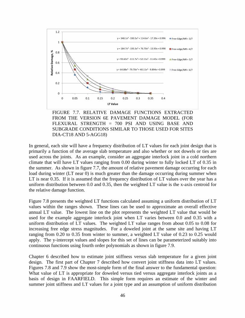
This research was performed under the Innovative Pavement Research Foundation (IPRF) in cooperation with the Federal Aviation Administration (FAA) as project number IPRF-01-G-002-05-2. The project initiated in the fall of 2007 and was completed in the summer of 2011. This summary report is an abridged version of the full report developed for the IPRF study and highlights the key findings and recommendations. Refer to the full report for more details and analyses. A majority of the heavy duty pavements that support large aircraft are constructed with jointed portland-cement concrete (PCC) pavement. This project studied the structural behavior of in-service jointed PCC pavements in the context of new state of the art structural analysis and pavement thickness design tools being developed by the FAA. The behavior of the joints that connect concrete slabs together is complex. Understanding how these joints transfer heavy aircraft wheel loads from slab to slab was the focus of this study. Historically, the load transfer and stress reduction effects from joints in concrete pavements have not been directly simulated in structural analysis models used for pavement thickness design by the FAA (FAA AC 150/5320 versions 6D and 6E). Instead, simplified “free-edge” loading structural analysis is performed using single-slab models without joints and with loads placed along the un-restrained edge of the slab. The free-edge stresses that result are then empirically adjusted using a long-ago established standard 25% stress reduction factor to account for the ability of joints to transfer load. The reduced free-edge stress values from these models are then used in empirically calibrated pavement damage equations for design of slab thickness for airfield pavements (US Army Corps of Engineers 1946; Parker et al., 1979; Rollings 1989; Brill, 2010). Joint load transfer is not a constant but rather is a stochastic variable changing continually as a function of temperature, and degrading over time due to repeated loading. Hence a fundamental issue is whether or not to model these changes in load transfer as part of the design process, or to simply assign a simplified lower limit value, such as the 25% factor concept. The simplified 25% reduction factor has allowed the complex behavior of joints and the mathematics associated with characterizing joint behavior to be eliminated from the thickness design process. PCC pavement damage models have been calibrated to the “free-edge stress” analysis approach using field test sites. The current design philosophy can be considered a simplified mechanistic-empirical design procedure. Since the late 1900’s, modern non-destructive field evaluation devices and techniques, along with computer based structural analysis capabilities have revealed new insights on slab and joint behaviors. These new insights have forced the research and design community to critically re-examine the simplified “75% of free-edge stress” design approach, leading to this study.

2

1.1 PROJECT SCOPE The IPRF request for proposal document for this project included a list of questions that served as the basis for this study of joint load transfer behavior. The questions are as follows:

What is the genesis of the assumption that a partial load transfer of the load at a joint reduces flexural stress by 25%?

What were the variables examined that resulted in the adoption of the 25% value?

What variables used in the development of the current 25% assumption are valid and applicable to pavement design as it exists today?

How sensitive are the pavement thickness design protocols being used to the assumed load transfer variables?

Do the minimum design requirements dictate the thickness requirement?

Is it feasible to dictate the use of a “short duration” period of low load transfer for the design?

Under what conditions is there a difference in load transfer efficiency for a dowelled, tied, and plain contraction joint?

On a contraction joint, does the depth of saw cut impact the value of load transfer efficiency?

Is there an ambient environment regime where load transfer efficiency is nearly constant?

Is there an ambient temperature environment when load transfer efficiency has a minimum value?

Can ambient environment be a design variable? If so, what are the conditions that must be satisfied before a reasonable value for load transfer can be assigned?

What are the variables that affect the quantitative value of load transfer efficiency and are those variables equally significant?

If not equally significant, what variables can be ignored for the purpose of assigning a value for load transfer?

Is there a simple technique that can be employed to determine when aircraft gear configuration will significantly influence the quantitative value of load transfer efficiency?

Is there sensitivity in the thickness computation that is a result of the interaction between gear configuration, slab curling, slab warping, slab size and load transfer for a given set of variables?

What metric is best used to define and model joint load transfer when data are collected using a Falling Weight Deflectometer (FWD)?

When using the FWD is it necessary to correct for slab bending?

What dynamic loading is required to evaluate load transfer efficiency?

3

Clearly the list of questions regarding joint load transfer that led to this research project is broad in scope. In order to thoroughly evaluate these questions, the following tasks and milestones were accomplished:

Performed an extensive literature review regarding joint load transfer and the history of the 25% load transfer adjustment factor.

Recognized that joint stiffness is the key mechanistic parameter used in finite element method (FEM) pavement analysis models that controls load transfer characteristics of joints.

Recognized that there was no existing way of directly computing joint stiffness using FWD joint load test data, and developed a new procedure for calculation of joint stiffness.

Recognized this new method allowed two new ways of backcalculating apparent modulus of subgrade reaction along joint lines for a field test site.

Performed detailed full-day site evaluations at heavy-duty jointed concrete pavement test sites using advanced mechanistic pavement evaluation procedures.

Performed a detailed analysis of FWD data from the Denver International Airport (DIA) instrumented test site, the NAPTF CC2 test strip study, and highway test sites.

Documented the range of joint stiffness versus deflection load transfer efficiency trends expected for pavements between about 8 and 22 inches in thickness.

Documented the effects of curling and temperature changes on joint stiffness and load transfer behavior.

Developed a comprehensive joint stiffness prediction tool that can predict joint stiffness versus average slab temperature as a function of slab length and other design parameters for doweled joints and aggregate interlock joints.

Matched FEM models and Skarlatos/Ioannides slab edge response models to the computed joint load transfer responses from test sites.

Performed load transfer sensitivity studies using calibrated FEM and Skarlatos/Ioannides models for various sizes of single wheel loads and multiple wheel gears.

Established simplified methods for estimating an effective Load Transfer (LT) value for a joint design considering climate variations and the FAA pavement damage model.

1.2 RESEARCH APPROACH The research plan developed for this project included detailed structural evaluations at eleven heavy-duty airfield concrete pavement test sites in the USA across different climate zones. The evaluations included:

4

measuring deflections using a heavy-weight FWD, measuring slab end slopes for use in slab curling analysis, measuring slab rotations using accelerometers, and measuring changes in joint opening size.

The testing was repeated multiple times during the day to study the impact of joint opening and slab temperature changes on joint load transfer. The intensive 8-10 hour on-site evaluation procedure is non-destructive and required no pavement sampling. These detailed evaluations have highlighted key differences between field joint behavior and how joints have typically been simulated in modern pavement structural analyses. Figure 1.1 shows a joint cross section highlighting key joint behaviors that are not easy to simulate. Once a pavement joint fully cracks, a joint opening develops as the ends of the slabs pull apart. In addition, slab ends will typically develop some slight differential settlements, which will cause small vertical offsets to develop between adjacent crack face roughness features. Load transfer is typically higher when loading the low slab. Load transfer is lower when loading the higher slab due to this off-set slack effect. The joint opening size can change dramatically from summer to winter, ranging from completely closed to completely open in regions having large seasonal thermal variation and for longer slab lengths. Dowels and tie bars are often installed across the joints to reduce the effect of off-set slack and differential settlement and to keep joints stiffer during cold weather. In general, the joint opening size, the roughness and stiffness of the crack face contact, and the amount and type of steel present across the joint control how load is transferred from slab to slab through the joint.

High Slab:Stiffer Support

ButLower LTE

Low Slab:Softer Support

ButHigher LTE

Fault

Differential Settlement or Erosion

Opening

Starting at a Very Early Age:Low-Slab drops down and rests on High-Slab aggregate interlock

Off-set Slack

Crack Face Roughness

Aggregate Interlock Forces

FIGURE 1.1 ILLUSTRATION OF PAVEMENT JOINT BEHAVIOR The most important structural analysis aspect regarding joint load transfer is the vertical shear stiffness of the fault shaped deflection that occurs along the joint line due to loading. In modern pavement analysis software, the pavement joint stiffness is the analysis input parameter that

5

controls how much force is passed through joints. Defining how joint stiffness varies over time of day and seasonally was a primary focus of this research. When interpreting joint stiffness using FWD measurements, joint stiffness is best characterized as having the three following components:

kJ = kJ-D/s + kJ-AGG + kJ-Base , lb/in/in (1) where,

kJ = Total calculated joint stiffness from a joint load test, lb/in/in. kJ-D/s = Stiffness from discrete devices (dowels, ties,…) with stiffness, D, spacing, s. kJ-AGG = Stiffness contribution from PCC slab crack face aggregate interlock. kJ-Base = Apparent joint stiffness contribution caused by elastic solid base effects.

The base component is related to the amount of “apparent” shear force transferred across the joint that is caused by the elastic solid base or subbase behavior beneath the joints. kJ-Base is not a true component of joint stiffness, but the base effect may appear as contributing to the total joint stiffness when estimating stiffness using FWD slab deflections. It is difficult to account for this third “base/subbase” component of apparent deflection load transfer across joints. It is also difficult to separate out how much of the computed total joint stiffness is due to dowels versus the aggregate interlock along the crack face. The on-site mechanistic evaluations conducted across the USA resulted in a database of FWD deflection measurements and slab curling data for airfield concrete slabs in the 14 to 22 inch thickness range, for a wide range of joint conditions and types. From this database, practical guidelines for in-service structural joint stiffness values and load transfer adjustment factors were developed for use in the design of jointed concrete pavements. For over a decade, the FAA has been developing modern structural analysis tools to replace the long-used Westergaard free-edge stress equations and layered elastic half-space analysis methods (Parker et al., 1979; Brill, 1998; Kawa et al., 2002; Brill, 2010). The new FAA analysis tools incorporate FEM structural analysis. There are two primary FEM formulations that are currently supported by FAA; a single 30-ft x 30-ft flat-slab free-edge model being used for thickness design in the Version 6E FAARFIELD software, and a more detailed jointed model for research having up to nine-slabs, and the ability to simulate curling of the slabs and referred to as the FEAFAA software. The enhanced FEAFAA software uses linear elastic joints, where joint stiffness is modeled as a constant linear stiffness value. This research project had the overall goal of evaluating joint load transfer behavior at airfield test sites and developing recommendations for joint load transfer to be used with design procedures and modern single slab and multi-jointed-slab FEM analyses.

6

CHAPTER 2. BACKGROUND INFORMATION 2.1 DEFINITIONS The study of load transfer across joints in PCC pavement systems has been intensive in the past with a large body of literature available. Over the years, three widely-used definitions for load transfer at a pavement joint or crack have been developed that are most relevant to this study. These definitions are as follows:

Deflection-based Load Transfer Efficiency (LTE) =

L

U

(2)

Stress-based Load Transfer Efficiency (LTE) =

L

U

(3)

Percent of “Free-Edge Stress” Load Transferred (LT) =

F

LF

)( (4)

Where,

L = Deflection of the loaded side of the joint U = Deflection of the unloaded side of the joint L = Bending stress in the loaded slab U = Bending stress in the unloaded slab L = Bending strain in the loaded slab edge at the joint F = Bending strain for “Free-Edge” loading conditions

Current technology and equipment can accurately measure slab edge deflections and deflection load transfer efficiency using nondestructive load tests. However, accurately measuring the stress or strain in concrete slabs is quite difficult. Theoretical slab models or real slabs instrumented with strain gauges are necessary to get estimates of stress or change in stress, which is directly related to measurable strain. The Percent of Free Edge Stress Load Transferred (LT) concept evolved in direct support of airfield pavement design and is related to testing of instrumented slabs using embedded strain gages focused on measuring slab edge bending strain caused by heavy wheel loads. Often, the free-edge strain was not actually measured but was assumed to be equal to the sum of the loaded slab strain and the unloaded slab strain measured for a joint load test. It is this stress reduction LT concept that was the primary focus of this research. LT is best defined as the percent reduction of the free-edge load bending stress caused by the joint load transfer effect, or more specifically, joint stiffness. The Load Transfer Efficiency (LTE) concepts are different than LT and are more widely used because of current abilities to measure joint deflections and compare these joint deflections with deflections computed using FEM analysis of jointed pavements. The following paragraphs provide detailed descriptions of joint types commonly used in airfield concrete pavement designs. The corresponding joint types currently specified in FAA AC 150/5320-6E are shown in parenthesis:

7

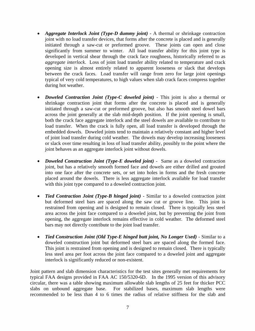
Aggregate Interlock Joint (Type-D dummy joint) - A thermal or shrinkage contraction joint with no load transfer devices, that forms after the concrete is placed and is generally initiated through a saw-cut or preformed groove. These joints can open and close significantly from summer to winter. All load transfer ability for this joint type is developed in vertical shear through the crack face roughness, historically referred to as aggregate interlock. Loss of joint load transfer ability related to temperature and crack opening size is almost entirely related to apparent looseness or slack that develops between the crack faces. Load transfer will range from zero for large joint openings typical of very cold temperatures, to high values when slab crack faces compress together during hot weather.

Doweled Contraction Joint (Type-C doweled joint) - This joint is also a thermal or

shrinkage contraction joint that forms after the concrete is placed and is generally initiated through a saw-cut or preformed groove, but also has smooth steel dowel bars across the joint generally at the slab mid-depth position. If the joint opening is small, both the crack face aggregate interlock and the steel dowels are available to contribute to load transfer. When the crack is fully open, all load transfer is developed through the embedded dowels. Doweled joints tend to maintain a relatively constant and higher level of joint load transfer during cold weather. The dowels may develop increasing looseness or slack over time resulting in loss of load transfer ability, possibly to the point where the joint behaves as an aggregate interlock joint without dowels.

Doweled Construction Joint (Type-E doweled joint) - Same as a doweled contraction

joint, but has a relatively smooth formed face and dowels are either drilled and grouted into one face after the concrete sets, or set into holes in forms and the fresh concrete placed around the dowels. There is less aggregate interlock available for load transfer with this joint type compared to a doweled contraction joint.

Tied Contraction Joint (Type-B hinged joint) - Similar to a doweled contraction joint

but deformed steel bars are spaced along the saw cut or groove line. This joint is restrained from opening and is designed to remain closed. There is typically less steel area across the joint face compared to a doweled joint, but by preventing the joint from opening, the aggregate interlock remains effective in cold weather. The deformed steel bars may not directly contribute to the joint load transfer.

Tied Construction Joint (Old Type-E hinged butt joint, No Longer Used) - Similar to a

doweled construction joint but deformed steel bars are spaced along the formed face. This joint is restrained from opening and is designed to remain closed. There is typically less steel area per foot across the joint face compared to a doweled joint and aggregate interlock is significantly reduced or non-existent.

Joint pattern and slab dimension characteristics for the test sites generally met requirements for typical FAA designs provided in FAA AC 150/5320-6D. In the 1995 version of this advisory circular, there was a table showing maximum allowable slab lengths of 25 feet for thicker PCC slabs on unbound aggregate base. For stabilized bases, maximum slab lengths were recommended to be less than 4 to 6 times the radius of relative stiffness for the slab and

8

foundation system. In the 2002 changes to Version 6D, a new note was added in the jointing requirements stating that joint spacing for all sites should be less than 20 feet unless the design engineer had good reason to allow longer slab dimensions. The 2002 version also recommended that joint spacing for stabilized bases be less than 5 times the radius of relative stiffness. In the current Version 6E of the advisory circular, joint spacing tables are provided for both stabilized and non-stabilized bases and no reference to radius of relative stiffness is present. The Version 6E tables limit joint spacing to be less than 20 feet. Therefore, in Version 6E, the 20-ft maximum joint spacing became a requirement and not a recommendation as it was in previous versions. The United States Air Force started using a maximum joint spacing of 20 feet in the mid 1980’s. This research project has verified that slab length is a critical parameter with respect to joint load transfer and slab curling stresses. Changing from 25-ft slab length to 20 feet results in up to 50 percent reduction in residual curling stresses, and will result in greater aggregate interlock. 2.2 BRIEF HISTORY OF THE 25% ADJUSTMENT FACTOR The unprecedented size of military aircraft used in World War II (WWII) forced the United States military to become actively involved in development of appropriate design and construction criteria for airfields. Since the 1940’s the military has played an active role in the airfield pavement arena as aircraft continued to evolve (Rollings, 2003; Ahlvin, 1991; Lenore and Remington, 1972). The FAA’s general design philosophy followed the military practices and only fairly recently have there been some divergence in design models and the approach used to establish the design requirements. In a series of tests during WWII, Corps of Engineers investigators established the current framework for military airfield rigid pavement design that included such salient features as:

The Westergaard models were used to predict strains and stresses in airfield pavement,

critical stresses were assumed to be caused by edge-loading adjacent to the joints,

slow moving or stationary aircraft were recognized to cause higher stresses than rapidly moving aircraft,

the importance of controlling non-load related curling stress was recognized,

repetitions of load were an important design factor, and

properly designed joints could reduce free edge strain by transferring load from one slab to another.

Following WWII through the Cold War and into the War on Terrorism, military airfield pavement design continued to evolve to meet changing needs and used theoretical development, small scale model tests, full-scale accelerated traffic tests, instrumented in-service pavements, and observation of airfield performance to support the evolution of design concepts (Rollings, 2003; Rollings and Pittman, 1992; Ahlvin, 1991; Rollings, 1989; Rollings, 1981; Hutchinson and

9

Vedros, 1977; Ahlvin et al., 1971; Hutchinson, 1966; Sale and Hutchinson, 1959; Mellinger and Carlton, 1955). A theoretical treatment of the load transfer issue was also developed by a doctoral student of Professor Westergaard under contract with the Army Corps of Engineers, but it received little attention until the mid 1990’s (Skarlatos, 1949; Ioannides and Hammons, 1996). This Skarlatos/Ioannides joint model was used extensively in this research. FAA and military design procedures did not evolve independently, but were intertwined from 1940 through the early 1990's with the military essentially establishing methodology and FAA accepting or modifying it to meet their needs. The Lockbourne and model tests of the 1940’s found that the Westergaard interior stress was not the critical state but edge stress was. The military funded Westergaard to help develop his revised free-edge stress equations (Westergaard, 1948). These equations were for single wheel load simulations and this is when the early models of the B-36 aircraft came out having a large 75,000 lb single wheel gear load. The 1948 Westergaard equations do not handle multiple-wheel loading configurations directly. Pickett and Ray (1950) eventually published their well-known multi-wheel influence diagram solution to Westergaard’s free-edge formulation. The Corps of Engineers used these influence diagrams to develop the pavement design curves of this era. Military design of this era used the Westergaard edge stress formulation for stress calculation, made adjustments for load transfer, and used available full scale traffic tests to relate the design factor (calculated stress and flexural strength) to coverages (cycles of stress at a point), which was a fatigue analysis. During the 1970’s, the layered elastic half-space analysis procedures for airfield pavements were developed (Parker et al., 1979). This design approach included an abstract calibrated procedure for estimating critical slab edge stress using analysis of a layered elastic half-space with no slab edges. Starting in about 1979, the FAA changed their official design criteria to be based on Westergaard’s free-edge stress equation in FAA AC 150/5320-6C (Barenberg and Arntzen, 1981) and variations of this approach have been used up to current times, until arrival of Version 6E and the single-slab three-dimensional FEM structural analysis model contained in the FAARFIELD software. The long established 25% stress reduction LT factor for joints has been incorporated in most of these pavement thickness design procedures.

10

CHAPTER 3. DEVELOPMENT OF TEST PLAN 3.1 KEY VARIABLES AFFECTING LOAD TRANSFER Based on an extensive literature review completed as a part of this study, the key variables related to joint stiffness and the load transfer characteristics of joints are provided below. The variables are divided into two sections. The first section contains the key primary variables that control the load transfer magnitude from a mechanistic perspective. The second section includes important secondary variables that cause variation in the effects of the primary mechanistic variables. In general, the joint stiffness is the key structural analysis parameter controlling how load is transferred through a pavement joint for a given pavement cross section. 3.1.1 Primary Variables affecting Load Transfer through PCC Slab Joints

1. Joint Opening- This is the primary factor controlling the effective joint stiffness for aggregate interlock joints without load transfer devices. At temperatures significantly below the casting temperatures for the concrete slabs, the joints will open and lose ability to transfer loads due to loss of aggregate interlock.

2. Joint Shear Face Roughness- The size, hardness, and durability of the shape irregularities that form along the crack faces will control aggregate interlock stiffness and how the joint responds to changes in joint opening size.

3. Joint Load Transfer Devices- Devices such as dowel and tie bars placed across joints help maintain load transfer ability during cold weather. Tied joints reinforced with deformed bars are designed to stay closed during cold weather and keep the cracks tightly together, keeping aggregate interlock high. Dowel-bars and tie-bars work in combination with aggregate interlock in the overall total joint stiffness response. When the joint opening becomes large enough to eliminate aggregate interlock, the dowel bar and its embedment zone support condition (modulus of dowel-concrete interaction, often called K or DCI) are the only joint load transfer mechanism.

4. Slab Thickness- There is a general trend of increasing joint stiffness for increasing slab thickness as the crack face area increases. However, there is also a general trend of lower achievable stress load transfer, LT, between slabs as the slab thickness increases. This is related to the fact that flexural rigidity of slabs increases in proportion with the slab thickness cubed, while the available joint shear area and joint stiffness only increases in proportion to slab thickness. Joints become relatively less efficient as slab thickness increases.

5. Slab Curvature- Changes in slab curvature from curling and warping does not directly affect joint stiffness, but does significantly affect the total joint deflections and overall load transfer behavior. Curling and warping can also cause residual tensile and laminar shear stresses to develop in slabs that will combine with wheel load stress and eventually may lead to cracking of the slabs due to fatigue.

11

6. Load Magnitude- Larger multi-wheel gears mobilize greater stress load transfer than smaller single wheel loads for a given joint stiffness condition.

3.1.2 Secondary Variables (Significant Cause Factors for Primary Variables)

1. Air Temperature- Typical daily and annual changes in air temperature are the primary cause for changes in the joint opening size and the slab curvature changes from curling.

2. Annual Precipitation and Humidity- In general, warping of concrete panels is related to

annual precipitation and humidity variations. Flatter slabs and smaller joint openings are associated with higher and more uniform precipitation rates.

3. Slab Length Relative to Thickness- For the same slab thickness, longer slabs will

develop larger joint openings and typically have greater curling deformations and residual thermal stresses in response to daily changes in temperature (Westergaard, 1927; Teller & Sutherland 1936; Finney & Oehler, 1959). Because typical airfield slabs are relatively short compared to their thickness, the slabs tend to curl relatively freely and have lower residual curling stress levels. Thermal gradient effects are expressed more in the form of deflection response than stress response for typical airfield pavements incorporating joint spacing less than 20 feet.

3.2 AIRFIELD TESTING PLAN After considering the key factors affecting joint load transfer and the capabilities of the FWD and other available tools for on-site evaluations, a comprehensive full-day mechanistic evaluation procedure was developed. The goal was to measure a site’s joint responses three times per day, sampled over the full daily thermal curling cycle, while quantifying curling. The on-site testing procedures included:

1. FWD Testing- A roughly square test site was established at each airfield typically six slabs by six slabs in size. An FWD test pattern was established and the pattern repeated typically three times from mid-morning to early-afternoon.

2. Slab Curvature (Curling) Measurements- Analysis of slab curling was accomplished using an analysis of the variation of slab end slopes. A DIPSTICK slope measurement device was used to obtain slope samples at ends of slabs. These values are used to quantify slab curvature changes occurring during testing.

3. Joint Opening Change Measurements- High resolution deflection measurement devices were epoxy mounted over joints to measure the change in joint opening, or “joint closure” that occurred during the testing window from mid-morning to early afternoon, relative to a zero value taken immediately after installation.

4. Slab Rotation Measurements- Two seismic geophones were set at the far edges of slabs during FWD joint load tests in attempt to quantify the dynamic uplift of the far slab edges that may occur as a result of slab rotation or tilting under load.

12

3.3 THE TEST SITES Figure 3.1 shows the general locations of the airfield test sites that were subjected to the full evaluation procedure. The locations of the additional DIA, NAPTF, and Road test sites that had useful pre-existing FWD data are also shown. The full airfield test sites are named starting with a number, 1 through 11, listed in order of decreasing mid-panel structural stiffness. The site number is followed by the base type code; AGG, CT, or AC for unbound aggregate base, cement treated base, or asphalt concrete base, respectively. The site base code is followed by a number representing the design slab thickness at the test sites. In general, coring of the pavement slabs in order to accurately measure slab thickness was not allowed. Therefore, this research relied on the “design thickness” as the basis for the assumed slab thickness for all analyses. The design thickness was obtained from construction plans for the test site areas. Figure 3.2 shows the pavement cross sections from design plans for the eleven full test sites.

✈

✈✈

✈

✈

2-AC17

DIA 1-AC18(22) & 4-AC18

✈

✈ ✈10-AGG14

5-AGG18

8-AGG15 & 11-CT14

3-CT16

6-CT16

✈

7-AGG17& 9-AGG14

✈NAPTF

Road-AGG10b

Road-CT8

Road-AGG10

Road-AGG9

FIGURE 3.1. MAP SHOWING GENERALIZED TEST SITE LOCATIONS

13

FIGURE 3.2. DESIGN CROSS SECTIONS FOR THE ELEVEN AIRFIELD TEST SITES

14

3.4 TEST EQUIPMENT AND PROCEDURES 3.4.1 Falling Weight Deflectometer Heavy-weight FWD devices were used as the primary joint structural behavior evaluation tool. FWD testing was performed using a Dynatest Model 8081 or similar FWD. This device is capable of applying loads in the range of 6,500 to 54,000 lb and recording the resulting pavement surface deflections at several locations at and near the applied load.

FIGURE 3.3. THE HEAVY-WEIGHT FALLING WEIGHT DEFLECTOMETER The FWD sensor set-up used was the typical seven-sensor line with sensors spaced at 12 inches apart from the center of the load plate, spanning a total distance of 72 inches. For the FWD joint load test, the deflection load transfer efficiency is defined as follows:

Deflection-based FWD Load Transfer Efficiency (LTE) = 100

6

6D

D (5)

Where, D-6 = Loaded slab load plate sensor deflection about 6 inches from joint D6 = Unloaded slab sensor deflection about 6 inches from joint

The FWD testing resulted in about 250 to 500 mid-slab load tests and 500 to 1000 joint load tests per site. This load versus deflection data was used to analyze and solve the Load Transfer (LT) problem. 3.4.2 The DIPSTICK Slope Measurements Slab shape changes caused by thermal curling were quantified using the FACE corporation DIPSTICK hand-held slope measurement device as shown in figure 3.5. This device is considered an ASTM Class A profiling device and provides an accurate way to measure slope

15

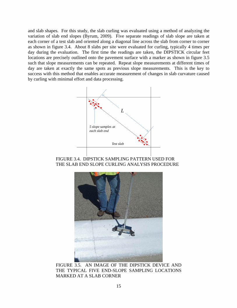
and slab shapes. For this study, the slab curling was evaluated using a method of analyzing the variation of slab end slopes (Byrum, 2009). Five separate readings of slab slope are taken at each corner of a test slab and oriented along a diagonal line across the slab from corner to corner as shown in figure 3.4. About 8 slabs per site were evaluated for curling, typically 4 times per day during the evaluation. The first time the readings are taken, the DIPSTICK circular feet locations are precisely outlined onto the pavement surface with a marker as shown in figure 3.5 such that slope measurements can be repeated. Repeat slope measurements at different times of day are taken at exactly the same spots as previous slope measurements. This is the key to success with this method that enables accurate measurement of changes in slab curvature caused by curling with minimal effort and data processing.

L

Test slab

5 slope samples ateach slab end

FIGURE 3.4. DIPSTICK SAMPLING PATTERN USED FOR THE SLAB END SLOPE CURLING ANALYSIS PROCEDURE

FIGURE 3.5. AN IMAGE OF THE DIPSTICK DEVICE AND THE TYPICAL FIVE END-SLOPE SAMPLING LOCATIONS MARKED AT A SLAB CORNER

16

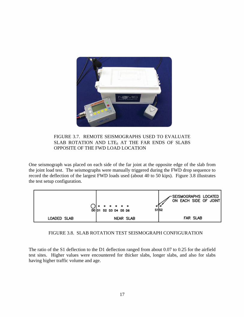
3.4.3 Measurement of Changes in Joint Opening Size Upon first arrival at the test site in the early morning, the joint opening sizes are about as large as they will be during the testing window. Shortly after arrival, brackets were epoxy mounted to each side of several joints in order to support digital deflection indicators having a 0.0001-inch resolution. These devices measured the change in joint opening, or “joint closure” that occurs from morning to afternoon during the site visit. Figure 3.6 shows a typical device set-up. FIGURE 3.6. MITUTOYO DIGITAL INDICATORS USED TO MEASURE THE CHANGES IN JOINT OPENING SIZE 3.4.4 Seismic Geophones for Slab Rotations The test routine also included measuring slab rotations during FWD testing. Slab rotation was measured by utilizing two additional Nomis Mini SUPERGRAPH seismographs as shown in figure 3.7. The seismographs are portable and measure frequency response with a seismic velocity range of 0 to 10 inches per second. The seismic velocity is then converted to deflection estimates using computer software that integrates the measured velocity data. The seismographs are similar to the velocity transducers used by the FWD device to quantify deflections.

17

FIGURE 3.7. REMOTE SEISMOGRAPHS USED TO EVALUATE SLAB ROTATION AND LTE AT THE FAR ENDS OF SLABS OPPOSITE OF THE FWD LOAD LOCATION

One seismograph was placed on each side of the far joint at the opposite edge of the slab from the joint load test. The seismographs were manually triggered during the FWD drop sequence to record the deflection of the largest FWD loads used (about 40 to 50 kips). Figure 3.8 illustrates the test setup configuration.

FIGURE 3.8. SLAB ROTATION TEST SEISMOGRAPH CONFIGURATION

The ratio of the S1 deflection to the D1 deflection ranged from about 0.07 to 0.25 for the airfield test sites. Higher values were encountered for thicker slabs, longer slabs, and also for slabs having higher traffic volume and age.

18

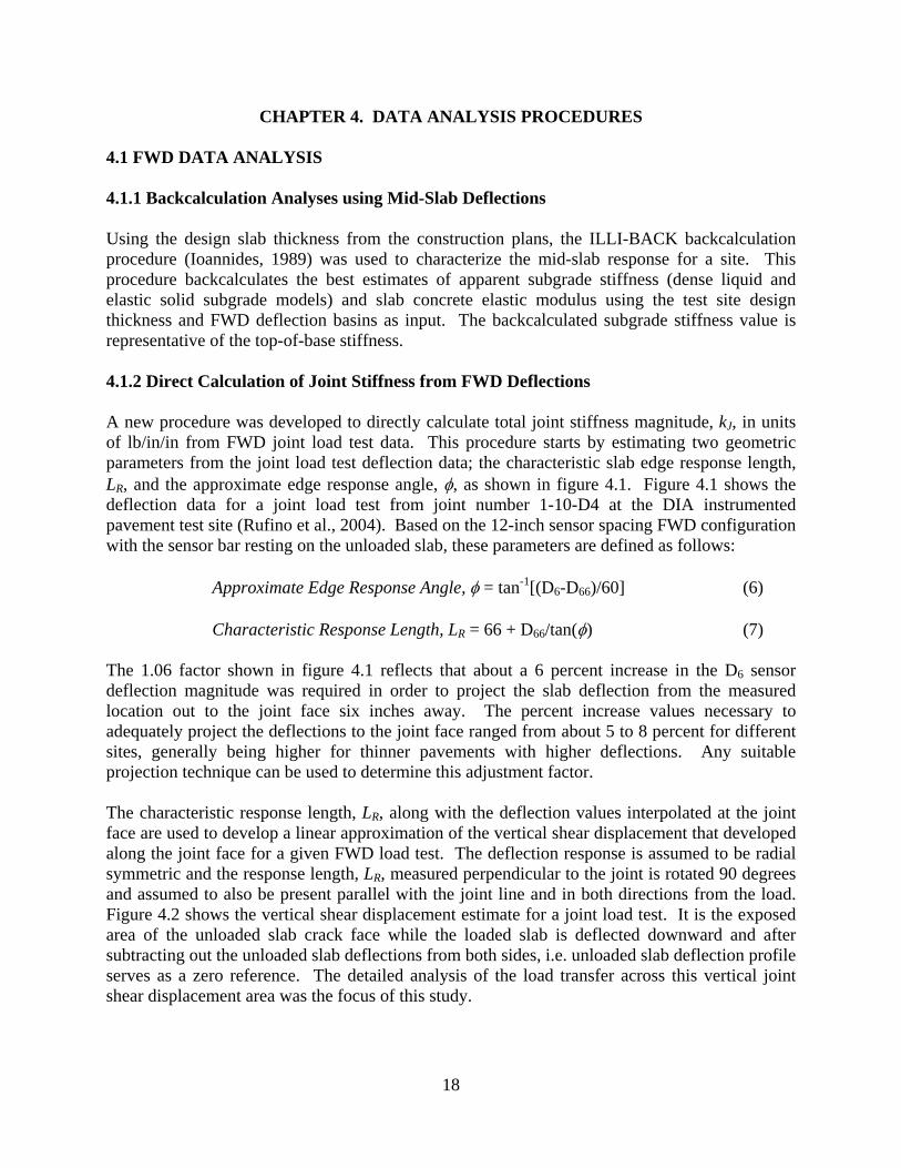
CHAPTER 4. DATA ANALYSIS PROCEDURES 4.1 FWD DATA ANALYSIS 4.1.1 Backcalculation Analyses using Mid-Slab Deflections Using the design slab thickness from the construction plans, the ILLI-BACK backcalculation procedure (Ioannides, 1989) was used to characterize the mid-slab response for a site. This procedure backcalculates the best estimates of apparent subgrade stiffness (dense liquid and elastic solid subgrade models) and slab concrete elastic modulus using the test site design thickness and FWD deflection basins as input. The backcalculated subgrade stiffness value is representative of the top-of-base stiffness. 4.1.2 Direct Calculation of Joint Stiffness from FWD Deflections A new procedure was developed to directly calculate total joint stiffness magnitude, kJ, in units of lb/in/in from FWD joint load test data. This procedure starts by estimating two geometric parameters from the joint load test deflection data; the characteristic slab edge response length, LR, and the approximate edge response angle, , as shown in figure 4.1. Figure 4.1 shows the deflection data for a joint load test from joint number 1-10-D4 at the DIA instrumented pavement test site (Rufino et al., 2004). Based on the 12-inch sensor spacing FWD configuration with the sensor bar resting on the unloaded slab, these parameters are defined as follows:

Approximate Edge Response Angle, = tan-1[(D6-D66)/60] (6)

Characteristic Response Length, LR = 66 + D66/tan() (7)

The 1.06 factor shown in figure 4.1 reflects that about a 6 percent increase in the D6 sensor deflection magnitude was required in order to project the slab deflection from the measured location out to the joint face six inches away. The percent increase values necessary to adequately project the deflections to the joint face ranged from about 5 to 8 percent for different sites, generally being higher for thinner pavements with higher deflections. Any suitable projection technique can be used to determine this adjustment factor. The characteristic response length, LR, along with the deflection values interpolated at the joint face are used to develop a linear approximation of the vertical shear displacement that developed along the joint face for a given FWD load test. The deflection response is assumed to be radial symmetric and the response length, LR, measured perpendicular to the joint is rotated 90 degrees and assumed to also be present parallel with the joint line and in both directions from the load. Figure 4.2 shows the vertical shear displacement estimate for a joint load test. It is the exposed area of the unloaded slab crack face while the loaded slab is deflected downward and after subtracting out the unloaded slab deflections from both sides, i.e. unloaded slab deflection profile serves as a zero reference. The detailed analysis of the load transfer across this vertical joint shear displacement area was the focus of this study.

19

0

5

10

15

20

25

30

-25 0 25 50 75 100 125 150

Distance from Joint, in

Defle

ctio

n,

mil

1-10-D4

D-6D6

D66

L R

(D-6- D6)1.06 = Vertical Joint Shear Displacementnear the Load

LOAD

Slab Plan View

jointLoadplate

FWD sensor

Deflection Profile

FIGURE 4.1. PLOT SHOWING THE FWD JOINT LOAD TEST DEFLECTION PROFILE CHARACTERISTICS, ALONG WITH THE EDGE RESPONSE ANGLE, , AND RESPONSE LENGTH, LR, FOR LOAD PLACED AT LOCATION D-6

LR LR

(D-6- D6)1.06

Joint Relative Shear Displacement Area Approximation

Unloaded Slab

LOAD

FIGURE 4.2. LINEARLY-APPROXIMATED JOINT VERTICAL SHEAR DISPLACEMENT PROFILE MOBILIZED ALONG THE JOINT FACE

In the context of joint stiffness (lb/in/in) the deflection difference profile along the joint is integrated to obtain the area of the deflection difference function, or shear area. This shear area is multiplied by the joint stiffness constant parameter, kJ, to obtain the total force mobilized and transferred through the joint. Using the geometry in figure 4.2, the total vertical force transmitted through the joint by shear is approximated as follows:

Total Joint Vertical Shear Force = ½ (2LR)(D-6-D6)1.06(kJ) (8)

20

The unknowns in the above equation are the joint stiffness value, kJ, and the total joint vertical shear force. The total joint shear force is not equal to the FWD load magnitude. Another separate equation is needed that can be solved for the Total Joint Vertical Shear Force variable to enable a final solution for the magnitude of joint stiffness. The LTE and FWD load magnitude can also be used to estimate the total joint vertical shear force. Figure 4.3 shows the simplified procedure for obtaining the necessary second equation for the total joint vertical shear force. The key assumption is that the overall subgrade resistance force, R, under each slab is proportional to the slab edge deflection.

P = FWD Drop Load

RR(LTE)

Joint Shear Force = R(LTE)

P = R + R(LTE)= R(1+LTE)

R = P/(1+LTE)

Subgrade Reaction“springs”

Total Joint Vertical Shear Force = P(LTE)/(1+ LTE)

FIGURE 4.3. SIMPLIFIED FORCE DISTRIBUTION MODEL FOR ESTIMATING THE TOTAL JOINT VERTICAL SHEAR FORCE

To calculate the total joint stiffness, kJ , the two equations for Total Joint Vertical Shear Force are set equal to each other and rearranged to solve for joint stiffness magnitude. The resulting equation to solve for kJ from FWD data using the 12-inch sensor spacing and sensor bar on the unloaded slab is as follows:

kJ = P(LTE)/[(1+LTE)(D-6-D6)(1 + i%)(66+60D66/(D6-D66))] (9) The i% factor is the percent increase factor needed to project the sensor readings out to the joint line. The term is an unknown function that converts the simplified linearly approximated shear area calculated above into the true shear area, and this function value was set equal to 1.0 for this study. The subscript values for the sensor deflections (i.e. D6, D-6, and D66) indicate the sensor distance, in inches, from the joint line. The equation’s geometry parameters must be adjusted to match any different FWD sensor configuration used. Testing many joints at a uniform test site and plotting the LTE versus joint stiffness data reveals the site’s characteristic joint stiffness versus LTE response trend associated with the site’s cross section properties. Plotting the characteristic joint stiffness data reveals information regarding joint type and cross section variability, along with any curling or joint opening effects that may

21

be occurring during the testing window. Figure 4.4 shows the computed joint stiffness data for site 2-AC17, which was resting on weak clay subgrade. Once the overall characteristic joint stiffness response trends are obtained from a test site, structural analysis models such as FEM jointed slab models or the Skarlatos/Ioannides infinite-edge model can be fit to these data. The FWD-based joint stiffness versus LTE curves obtained from the test sites are the primary data used as the basis for the recommendations resulting from this research project. In general, prior to establishing a method as described above for calculating joint stiffness directly from FWD load test data, it was not possible to develop such information for a test site.

0%

10%

20%

30%

40%

50%

60%

70%

80%

90%

100%

0 50000 100000 150000 200000 250000 300000

LTE

-del

ta

Joint Stiffness, lb/in/in

Site 2-AC17

6:00-9:30 AM

9:45-11:30 AM

11:45-1:45 PM

LTE= 89%

Possible Un-Cracked/Locked Joints 13%

All Joints Median = 125,300 lb/in/in at 79% LTE

Without locked/uncracked:Median = 113,600 lb/in/in at 78% LTE

FIGURE 4.4. AN EXAMPLE OF RELATIVELY UNIFORM JOINT STIFFNESS RESPONSE FOR A HEAVY DUTY RUNWAY HAVING WEAK CLAYEY SUBGRADE

4.1.3 Fitting the Skarlatos/Ioannides Model to the Characteristic Joint Stiffness Data There are two forms of the Skarlatos/Ioannides load transfer regression equations (Ioannides & Hammons, 1996) that can be used with the computed joint stiffness versus LTE characteristic data. These equations simulate two infinite slabs connected by one infinitely long joint. These equations can easily be “fit” to the FWD-based joint stiffness data from a site. One form is demonstrated here and is referred to as the “LTE regression for the Skarlatos/Ioannides model” shown below:

22

(10)

Where,

kJ = AGG = q0 = joint stiffness, lb/in/in

= wheel load radius, inches ℓ = pavement radius of relative stiffness, inches k = modulus of subgrade reaction, psi/in

For each test site, the FWD-based joint stiffness versus LTE data is set up to solve the following generalized matrix equation:

[Measured LTE] = [Skarlatos LTE as f(site best-fit kℓ )] + [error] (11) A computer optimization routine is used to find the single best-fit slab-edge modulus of subgrade reaction (k-value) for the site that minimizes the sum of squared errors for the error matrix. The field measured data, the design thickness, the estimated slab elastic modulus, and the LTE form of the Skarlatos/Ioannides model are used in the minimization problem to find the best-fit subgrade k-value at the joints with typical model fit as shown in figure 4.5. This is a new rational backcalculation method for apparent slab edge support magnitude for a test site using the general assumptions of dense liquid foundation and two semi-infinite slabs with a single infinite joint. It is referred to as the “Backcalculated Skarlatos Infinite Edge Modulus of Subgrade Reaction Value”, or kSkarlatos. Because the Skarlatos/Ioannides/Westergaard model assumes infinite slab dimensions along and away from the joint line, the backcalculated kSkarlatos represents a lower bound solution for the support magnitude at joints.

23

0

10

20

30

40

50

60

70

80

90

100

0% 20% 40% 60% 80% 100%

Ska

rlat

os

LT

E, %

Measured LTE

Site 2-AC17Skarlatos Equation Matching LTE :Best-f it Joint Subgrade k = 200 psi/inchEC = 6,440,000 psiPCC Thickness = 17 inches

FIGURE 4.5. BEST-FIT SKARLATOS/IOANNIDES LTE REGRESSION MODEL FOR SITE 2-AC17

The Skarlatos/Ioannides model above with a kSkarlatos = 200 psi/in is considered the “calibrated” Skarlatos/Ioannides LTE joint behavior model that best reproduces the computed joint stiffness data from site 2-AC17. It should be noted that the method used to calculate joint stiffness values from the site is not related to the Skarlatos/Ioannides equation. The relatively good fit between the measured LTE and the Skarlatos predicted LTE when using the computed stiffness data from this new technique is an indication that in-service joint behavior at this test site is very much like Skarlatos predicted it would be. The overall site 2-AC17 average mid-panel backcalculated modulus of subgrade reaction from ILLI-BACK was 430 psi/in. Therefore, the Skarlatos/Ioannides infinite edge type Slab Support Ratio calculated for site 2-AC17 is 200/430 or about 0.47. 4.1.4 Fitting a Finite Element Model to the Characteristic Joint Stiffness Data To evaluate factors such as slab length variations or slab curling effects, FEM analyses of jointed slabs was performed. This study primarily used the FEM software ILSL2 (Ioannides & Khazanovich, 1998), to match computed responses with the test site response data. The design slab thickness and the ILLI-BACK determined slab concrete elastic modulus value were used for the slab properties in the FEM models. In general, the ILLI-BACK mid-panel backcalculated subgrade k-value represents an upper bound for subgrade stiffness expected to be present at joints, while the backcalculated Skarlatos/Ioannides infinite slab edge subgrade k-value represents a lower bound solution for the support at joints. Figure 4.6 shows the characteristic joint stiffness data from site 2-AC17, along with Skarlatos/Ioannides and ILSL2 joint stiffness curves for the upper and lower bound subgrade k-values of 200 and 430 psi/in. The Skarlatos/Ioannides model with a subgrade k-value of 200 psi/in was the best-fit model and runs through the center of the FWD data population. The best-fit FEM model has a subgrade k-value of about 375 psi/in. These calibrated response models fit to the measured data are based on the FWD load plate size. These calibrated models can be used to infer trends for other load area

24

sizes or multi-wheel gears and to calculate apparent load transfer percentages for a wide range of conditions and simulations.

0%

10%

20%

30%

40%

50%

60%

70%

80%

90%

100%

0 50000 100000 150000 200000 250000 300000

LTE

-del

ta


Site 2-AC17

6:00-9:30 AM

9:45-11:30 AM

11:45-1:45 PM

ILSL2, k=200 flat

ILSL2, k=430 flat

Skarlatos LTE k = 200

Skarlatos LTE k = 430

ILSL2, k=375 flat

LTE>89% = locked/un-cracked

FIGURE 4.6. PLOT SHOWING HOW THE BEST-FIT SKARLATOS/IOANNIDES SLAB EDGE SUBGRADE k-value (200 PSI/IN), AND THE ILLI-BACK MID-PANEL SUBGRADE k-value (430 PSI/IN) ACT AS UPPER AND LOWER FEM SOLUTION BOUNDARIES, WITH BEST-FIT ILSL2 FEM k-value AT ABOUT 375 PSI/IN

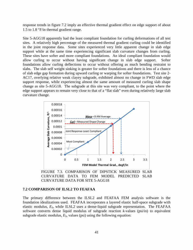
4.2 SLAB CURLING AND WARPING ANALYSIS PROCEDURE Slab curling and warping were evaluated using a method for analyzing the variation of slab end slopes (Byrum, 2009). Figure 4.7 shows an example of results for test slabs from site 5-AGG18, along with summary data from a 500-ft long highway site 55-3009. There is considerable variation in the average value of curvature, or apparent locked-in warp, in each of the slabs represented as lines on the plot. Both test sites had a range of average slab curvatures (warp) of about 0.0009 ft-1, and this is a typical range for a relatively uniform test site. Finishing and texture also affect the average slab curvature (warp) measurement from slab to slab. The overall site average slab curvature present just after sunrise, when the effective linear portion of the thermal gradient reaches zero magnitude, is the approximate locked-in warp value. The change in curvature measured in each slab is shown to be nearly identical and this change in curvature is the curling effect. To demonstrate the precision of the estimate for the curling related change in curvature at site 5-AGG18, the average curvature change from the seven slabs was about 0.000111 ft-1. The standard error for this mean value is estimated as; the standard deviation of the curvature change values (0.000012 ft-1) divided by the square root of seven or

25

approximately 0.0000045 ft-1. The standard error is about 4% of the typical range of curling related slab curvature change, which can be as high as 0.0001 to 0.0002 ft-1 change from mid-morning to early-afternoon on thermally active days. Therefore, the measured average curvature change caused by curling is a good estimate of the true mean value of curling with seven slabs as its basis. The overall 8 AM approximate average slab curvature from the seven slabs was about 0.00013 ft-1, with a positive value meaning upward curvature or joints lifted. This is the approximate locked-in warp magnitude at the test site.

500-ft Highway Site 5-AGG18GPS3 55-3009 8AM average AM-PM Change

average curvature, 1/ft 0.000547 0.000126 0.000111min. curvature 0.000203 -0.000362 0.000089max. curvature 0.001077 0.000555 0.000124

st. dev. of curvature 0.00021 0.000287 0.000012number of slabs 33 7 7

‐0.0006

‐0.0004

‐0.0002

0

0.0002

0.0004

0.0006

0.0008

6:00 AM 8:00 AM 10:00 AM 12:00 PM 2:00 PM 4:00 PM 6:00 PM

Slab

Curvature, 1/ft

Approximate Time of DIPSTICK Slope Reading

Site 5‐Agg18: Per Slab Curvature Data

FIGURE 4.7. TYPICAL RESULTS OF DIPSTICK SLAB END SLOPE CURLING AND WARP ANALYSIS

26

CHAPTER 5. RANGE OF OBSERVED JOINT BEHAVIOR Figure 5.1 shows the overall summary plot of the FWD-based joint stiffness data obtained from the test sites. This is the primary data set used as the basis for recommendations derived from this research. Each site has a considerable range of LTE and joint stiffness values that follow the general Skarlatos/Ioannides-type trend shape. Although this plot is too cluttered to assess any individual site well, there is a strong basic trend in this data related to pavement cross section. The thinner 8-11 inch slabs occupy the upper and left portion of the plot while the heavy duty 17-22 inch thick slabs occupy the lower right portion of the plot. At a joint stiffness value of about 50,000 lb/in/in, an 18-22 inch slab was revealing an LTE of about 63%, while a 9-10 inch slab has an LTE of about 85%. The apparent warm weather joint “lock-up” stiffness values (at LTE of about 86 to 90 percent) are about 100,000 and 250,000 lb/in/in for the 10 and 20 inch slab thickness, respectively.

30%

40%

50%

60%

70%

80%

90%

100%

0 50000 100000 150000 200000 250000

LTE‐delta


1‐AC18(22)‐a

1‐AC18(22)‐b

DIA‐CT18

2‐AC17

3‐CT16

4‐AC18‐a

4‐AC18‐b

5‐AGG18

6‐CT16

7‐AGG17

8‐AGG15

9‐AGG14

10‐AGG14

11‐CT14

NAPTF‐CT11, new

NAPTF‐CT11, failed

Road2‐AGG10

Road3‐AGG10

Road1‐AGG9

FIGURE 5.1. THE JOINT STIFFNESS DATA FROM THE TEST SITES (kJ<250 KIP/IN/IN, LTE > 30%, 5.91 INCH RADIUS FWD LOAD PLATE)

27

The joint load test data from the test sites was further broken down to individual joint types and by Round of testing as shown in figure 5.2 for test site 5-AGG18. This test site is within a heavy duty runway landing zone area. The transverse doweled joints are saw-cut joints and are confined in both directions by hundreds of feet of additional concrete slabs. The runway is only 6 slabs wide so the longitudinal joints are not nearly as confined as the transverse joints. The longitudinal joints have flat construction joint faces and it appears that the faces began to lock-up during the Round 3 testing. However, during Round 1 and Round 2, the faces may have been disengaged, with the joint stiffness mobilized primarily through the dowels. The transverse saw-cut joints with dowel bars appear to have had greater mobilization of aggregate interlock in the morning, with increasing aggregate interlock as temperatures increased. The slab corner tests showed the most sensitivity to time of day as the thermal expansion and contraction occurs in two dimensions at the corners and is magnified.

0

20000

40000

60000

80000

100000

120000

140000

160000

180000

T. Doweled Contraction

L. Doweled Contraction

L. Doweled Construction

Corners

Avg. Joint Stiffness, lb/in/in

Site 5‐AGG18

AM

Late AM

Early PM

FIGURE 5.2. BEHAVIOR OF INDIVIDUAL JOINT TYPES AT SITE 5-AGG18

Figures 5.3 and 5.4 show the winter and summer testing results for site 1-AC18(22). During winter, there was a steady increase in joint stiffness during testing indicating about 25,000 lb/in/in of aggregate interlock had mobilized in addition to the stiffness level that was present during morning testing. It is unclear as to how much of the morning joint stiffness of about 60,000 lb/in/in is from dowels versus aggregate interlock. Corner stiffness remained low during winter indicating that aggregate interlock was only just starting to mobilize, if any, at corners. Both joint types had reached about 90,000 lb/in/in stiffness during the winter afternoon testing. The summer testing revealed that as a result of continued joint closure, total joint stiffness had risen to about 120,000 lb/in/in for the contraction joints, but had stayed at about 90,000-100,000 lb/in/in for the construction joints. This is an indication that the available aggregate interlock for the construction joints was limited compared to that available for the naturally cracked contraction joints. During summer testing, the corners appear as stiff as the joints, whereas during winter the corner stiffness was much softer than the joints.

28

0

20000

40000

60000

80000

100000

120000

140000

160000

AM Late AM Early PM


Site 1‐AC18(22); Winter 2009

Doweled Construction

Doweled Contraction

Corners

FIGURE 5.3. BREAKDOWN OF JOINT STIFFNESS BY JOINT TYPE AND ROUND OF TESTING FOR SITE 1-AC18(22) FOR WINTER OF 2009

0

20000

40000

60000

80000

100000

120000

140000

160000

AM Late AM Early PM


Site 1‐AC18(22); Summer 2010

Doweled Construction

Doweled Contraction

Corners

FIGURE 5.4. BREAKDOWN OF JOINT STIFFNESS BY JOINT TYPE AND ROUND OF TESTING FOR SITE 1-AC18(22) FOR SUMMER OF 2010

Corners were not tested during the “Early PM” in the summer of 2010. Detailed breakdowns of the joint behaviors such as these allowed a better understanding of the relative contributions of dowels versus aggregate interlock in terms of the total joint stiffness. The analyses also allowed development of plots such as figure 5.5, which provides a summary of the median and minimum computed joint stiffness values for the doweled joint types from the test sites.

29

0

25000

50000

75000

100000

125000

150000

175000

200000


Doweled Joint Stiffness Summary Median

Minimum

FIGURE 5.5. MEDIAN AND MINIMUM JOINT STIFFNESS VALUES FOR DOWELED JOINT TYPES (L = LONGITUDINAL, T = TRANSVERSE, CN = CONSTRUCTION, CT = CONTRACTION)

The direct joint stiffness determination procedure has enabled backcalculation of the modulus of dowel-concrete interaction factors for the doweled joints from the test sites. The results are provided in figure 5.6. The overall test group average modulus of dowel-concrete interaction, K, matching the site median joint stiffness values was about 3,100,000 psi. The overall test group average modulus of dowel-concrete interaction value matching the minimum FWD-based joint stiffness values obtained for the various joint types was about 810,000 psi.

0

2,000,000

4,000,000

6,000,000

8,000,000

10,000,000

Dowel‐Concrete Interaction (K) psi/in

Max Possible Dowel‐Concrete Interaction, K*completely ignoring possible aggregate interlock

Median

Minimum

FIGURE 5.6. SUMMARY OF BACKCALCULATED MODULUS OF DOWEL-CONCRETE INTERACTION VALUES MATCHING THE MEDIAN AND MINIMUM JOINT STIFFNESS VALUES FROM FIGURE 5.5

30

CHAPTER 6. MODELING THE OBSERVED JOINT BEHAVIOR Two joint behavior prediction tools were developed under this study to reproduce the joint stiffness behaviors observed in the field and for use in pavement design:

1. A simplified model that allows the development of the characteristic joint stiffness response curve for a design. Output from this procedure consists of estimated joint stiffness versus LTE.

2. A comprehensive joint model that predicts joint behavior as a function of more factors such as joint opening size, slab temperature, slab length, materials variations, and traffic, for both doweled and aggregate interlock joints. The detailed model output consists of joint stiffness and LTE as a function of slab temperature.

6.1 SIMPLIFIED METHOD FOR PREDICTING THE CHARACTERISTIC JOINT STIFFNESS CURVE To establish the joint stiffness versus LTE prediction model, Skarlatos/Ioannides edge response curves were fit to the entire computed joint stiffness versus LTE data set displayed in figure 5.1. The slab thickness values in the Skarlatos/Ioannides curves were varied over the range of 7 to 22 inches. The concrete elastic modulus values were fixed at 5,000,000 psi for all curves. Then, the slab edge subgrade k-values were varied in the Skarlatos/Ioannides equations until the set of Skarlatos/Ioannides curves were back-predicting the general thickness related trend observed in the computed joint stiffness data. Figure 6.1 shows the three resulting Skarlatos/Ioannides control curves for the simplified model. The Skarlatos/Ioannides model subgrade k-values of 120, 180, and 240 psi/in can be considered empirically calibrated edge support values that force the Skarlatos Equation developed by Ioannides & Hammons, 1996 to fit the computed data, while assuming a constant slab elastic modulus of 5,000,000 psi. The banded zone highlighted around an LTE value of 90 percent is the zone where the joint stiffness trend lines become relatively asymptotic with respect to LTE. Significant slab bending moment is being transmitted across joint faces for high LTE values above this transition zone and the concept of linear joint stiffness becomes invalid.

31

30%

40%

50%

60%

70%

80%

90%

100%

0 50000 100000 150000 200000 250000

LTE‐delta


1‐AC18(22)‐a

1‐AC18(22)‐b

DIA‐CT18

2‐AC17

3‐CT16

4‐AC18‐a

4‐AC18‐b

6‐CT16

7‐AGG17

8‐AGG15

10‐AGG14

11‐CT14

NAPTF‐CT11, new

NAPTF‐CT11, failed

Road2‐AGG10

Road3‐AGG10

Road1‐AGG9

Skarlatos, k=120, H=7"



FIGURE 6.1. THE THREE SKARLATOS CURVES USED FOR ESTIMATING A SITE SPECIFIC CHARACTERISTIC JOINT STIFFNESS CURVE FOR FWD LOADING

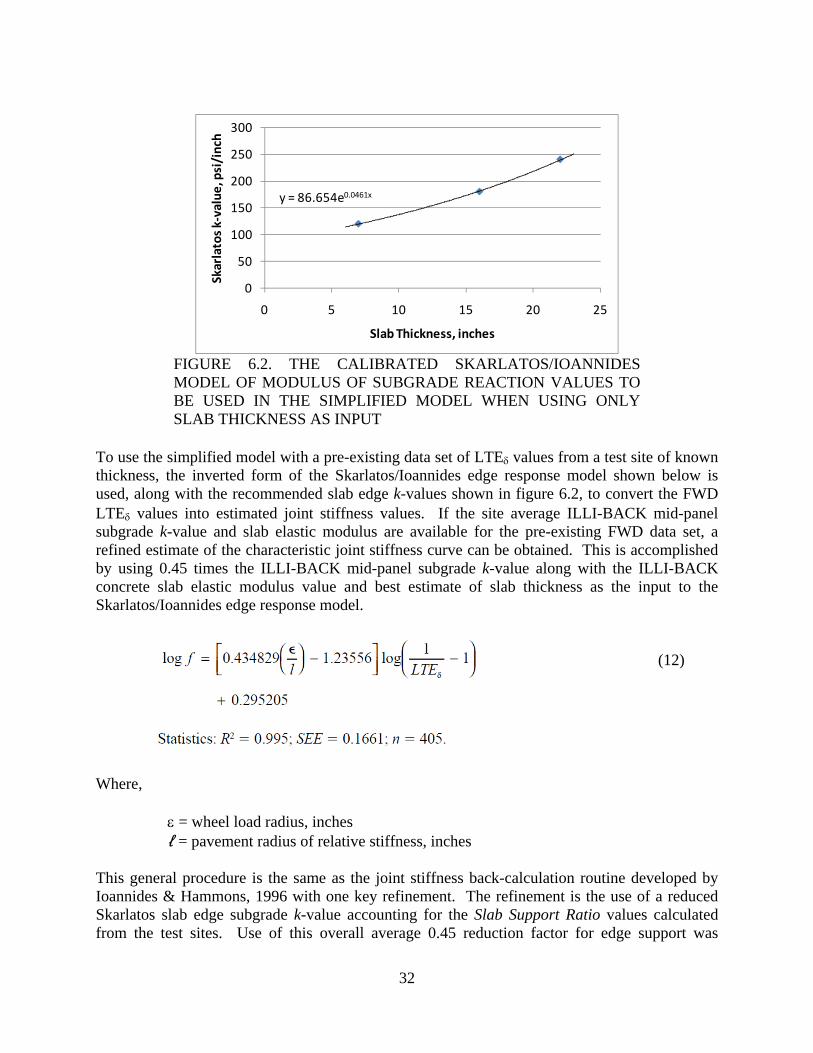
The recommended slab edge subgrade k-values to be used in the simplified model when only an estimate of slab thickness is available are shown in figure 6.2. Use of these values will simulate newer pavement conditions with slightly less wear and slightly higher slab support ratio values than observed at the in-service test sites. Aging and loss of support will reduce effective slab support ratio values. This “effect” can be simulated by reducing the slab edge subgrade k-value in the Skarlatos/Ioannides model for a given slab thickness.

32

y = 86.654e0.0461x

0

50

100

150

200

250

300

0 5 10 15 20 25

Skarlatos k‐value, psi/inch

Slab Thickness, inches

FIGURE 6.2. THE CALIBRATED SKARLATOS/IOANNIDES MODEL OF MODULUS OF SUBGRADE REACTION VALUES TO BE USED IN THE SIMPLIFIED MODEL WHEN USING ONLY SLAB THICKNESS AS INPUT

To use the simplified model with a pre-existing data set of LTE values from a test site of known thickness, the inverted form of the Skarlatos/Ioannides edge response model shown below is used, along with the recommended slab edge k-values shown in figure 6.2, to convert the FWD LTE values into estimated joint stiffness values. If the site average ILLI-BACK mid-panel subgrade k-value and slab elastic modulus are available for the pre-existing FWD data set, a refined estimate of the characteristic joint stiffness curve can be obtained. This is accomplished by using 0.45 times the ILLI-BACK mid-panel subgrade k-value along with the ILLI-BACK concrete slab elastic modulus value and best estimate of slab thickness as the input to the Skarlatos/Ioannides edge response model.

(12)

Where,

= wheel load radius, inches ℓ = pavement radius of relative stiffness, inches

This general procedure is the same as the joint stiffness back-calculation routine developed by Ioannides & Hammons, 1996 with one key refinement. The refinement is the use of a reduced Skarlatos slab edge subgrade k-value accounting for the Slab Support Ratio values calculated from the test sites. Use of this overall average 0.45 reduction factor for edge support was

33

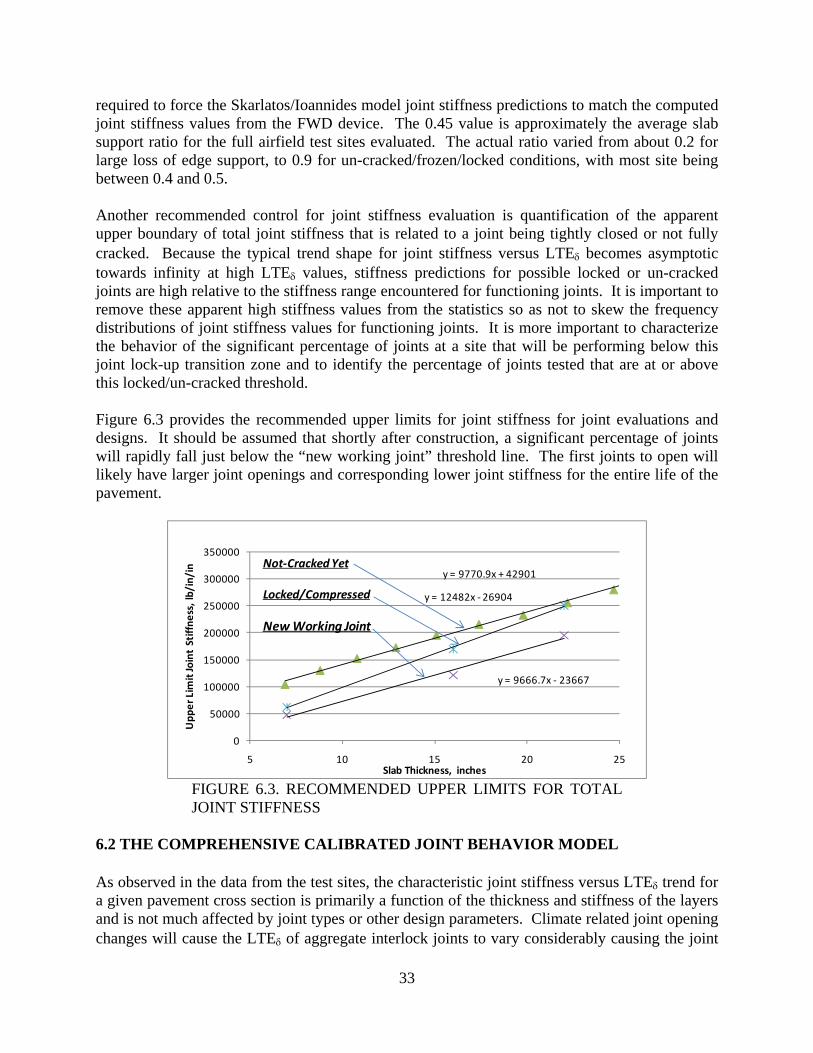
required to force the Skarlatos/Ioannides model joint stiffness predictions to match the computed joint stiffness values from the FWD device. The 0.45 value is approximately the average slab support ratio for the full airfield test sites evaluated. The actual ratio varied from about 0.2 for large loss of edge support, to 0.9 for un-cracked/frozen/locked conditions, with most site being between 0.4 and 0.5. Another recommended control for joint stiffness evaluation is quantification of the apparent upper boundary of total joint stiffness that is related to a joint being tightly closed or not fully cracked. Because the typical trend shape for joint stiffness versus LTE becomes asymptotic towards infinity at high LTE values, stiffness predictions for possible locked or un-cracked joints are high relative to the stiffness range encountered for functioning joints. It is important to remove these apparent high stiffness values from the statistics so as not to skew the frequency distributions of joint stiffness values for functioning joints. It is more important to characterize the behavior of the significant percentage of joints at a site that will be performing below this joint lock-up transition zone and to identify the percentage of joints tested that are at or above this locked/un-cracked threshold. Figure 6.3 provides the recommended upper limits for joint stiffness for joint evaluations and designs. It should be assumed that shortly after construction, a significant percentage of joints will rapidly fall just below the “new working joint” threshold line. The first joints to open will likely have larger joint openings and corresponding lower joint stiffness for the entire life of the pavement.

y = 9770.9x + 42901

y = 9666.7x ‐ 23667

y = 12482x ‐ 26904

0

50000

100000

150000

200000

250000

300000

350000

5 10 15 20 25

Upper Limit Joint Stiffness, lb/in/in

Slab Thickness, inches

Not‐Cracked Yet

Locked/Compressed

New Working Joint

FIGURE 6.3. RECOMMENDED UPPER LIMITS FOR TOTAL JOINT STIFFNESS

6.2 THE COMPREHENSIVE CALIBRATED JOINT BEHAVIOR MODEL As observed in the data from the test sites, the characteristic joint stiffness versus LTE trend for a given pavement cross section is primarily a function of the thickness and stiffness of the layers and is not much affected by joint types or other design parameters. Climate related joint opening changes will cause the LTE of aggregate interlock joints to vary considerably causing the joint

34

stiffness magnitude to drift back and forth along nearly the full range of the characteristic joint response trend from summer to winter. Adding dowels will keep LTE higher during winter, resulting in less movement back and forth along the characteristic joint stiffness trend. The analysis of the joint stiffness data indicated that a comprehensive joint stiffness behavior model that included the primary mechanistic joint behavior parameters was needed in order to simulate significant effects caused by slab temperature variations. Past research has shown that LTE tends to have a relatively linear trend with respect to average slab temperature, with slope d(LTE)/dT (Prozzi et al., 1993; Kazahnovich & Gotlif, 2003). The magnitude of the rate of change is related primarily to slab length and roughness/tortuosity of the crack face. A rough crack face or a short slab will have a flatter LTE versus temperature slope, whereas a smooth face or long slab will have a steep slope, or sudden loss of LTE with slab thermal contraction. The TLock temperature is the point at which the joint faces completely compresses shut and full “locked” joint stiffness is mobilized. The TRelease temperature is the point at which the joint faces no longer have shear contact while deflecting under loads, and joint stiffness due to aggregate interlock is zero. The new comprehensive joint behavior model predicts the TLock and TRelease temperatures and the LTE thermal rate of change for a given aggregate interlock joint design. This model also uses a “calibrated” doweled joint model combined with the aggregate interlock model to simulate dowel effects. The calibrated Skarlatos/Ioannides edge models are then matched to the predicted linear LTE versus temperature trends to estimate joint stiffness trends as a function of slab temperature for a given pavement design. Existing joint opening models can be used to estimate the magnitude of another key derivative, dO/dT, the change in joint opening size, O, as a function of temperature and slab dimensions. Past research has shown that this derivative function is also generaly linear with respect to temperature. Therefore, the d(LTE)/dT constant can simply be divided by the dO/dT constant to get the variable d(LTE)/dO for the aggregate interlock component of a given joint design. This is a key parameter, d(LTE)/dO, for aggregate interlock joints and represents the change in LTE with respect to change in joint opening size. At DIA, the d(LTE)/dO parameter was carefully measured and the aggregate interlock joints were found to experience approximately 0.9 to 1.3 percentage point loss in LTE for each 1 mil increase in joint opening. For purposes of this research, a loss rate of 1.3 LTE percent for each 1 mil of joint opening is considered an average typical loss rate for sawed joint crack face conditions. The Michigan Department of Transportation (MDOT) joint opening model was selected to predict the assumed dO/dT magnitude as a function of design slab length (Finney and Ohler, 1959). The detailed measurements at DIA form the model’s assumed basis for the typical LTE loss rate, d(LTE)/dO, for aggregate interlock. The 17 years of joint opening size measurements by MDOT form the basis of the model’s assumed joint opening rate, dO/dT, as a function of slab length. These two expressions are then divided to obtain the LTE change rate with respect to temperature, d(LTE)/dT, for various joint designs. Figure 6.4 shows the joint behavior presentation scheme used for the final comprehensive joint behavior model. This figure represents the calibrated DIA joint behavior model. The solid lines in the lower plot represent

35

aggregate interlock joints, while the dashed lines represent doweled joint behavior. In cold temperatures, doweled joint stiffness is controlled by the dowel component of total stiffness, while the aggregate interlock component drops to zero for open joints.

y = 1.266x ‐ 22.319

0

10

20

30

40

50

60

70

80

90

0 20 40 60 80 100 120

LTE‐delta, %

Average Daily Temperature, degF

Predicted LTE vs. Temperature

New Agg. Joint LTE‐delta

Aged Agg. Joint LTE‐delta

DIA Avg Agg Dummy Joint

0

50000

100000

150000

200000

250000

0 20 40 60 80 100 120


Average Daily Temperature, degF

Predicted Joint Stiffness vs. Temperature

New Agg Joint

Aged Agg Joint

New Doweled Joint

Aged Doweled Joint

FIGURE 6.4. THE COMPREHENSIVE JOINT MODEL PREDICTS LTE AS A FUNCTION OF SLAB TEMPERATURE AND THEN USES THE CALIBRATED SKARLATOS/IOANNIDES EDGE MODEL AND THE FAA DOWELED JOINT MODEL TO PREDICT JOINT STIFFNESS VERSUS SLAB TEMPERATURE

Figure 6.5 shows the estimated variation of joint stiffness for doweled and aggregate interlock joints for a simulated annual sine-wave temperature range with overall variation similar to the climate at DIA. The new-condition joint simulations provide good estimates of how joint

36

stiffness varied at DIA based on close matches to the measured data from that site. The end-of-life joint simulation includes projections of how joints will deteriorate over time. The end-of-life predictions reflect the amount of dowel-concrete interaction and aggregate interlock loss that was observed in test sections of various age. In general, it is not known at this time how loss of joint stiffness develops as a function of age. However, it has been observed that doweled joints can lose stiffness substantially with accumulating age and traffic. The flat top for the doweled joint lines represents the upper-limit of joint stiffness recommended for the 18 inch slab thickness at DIA (see figure 6.3).

0

50000

100000

150000

200000

250000

0 50 100 150 200 250 300 350 400


Day of the Year

Age = 0 Joint Behavior

Avg Agg. Int.

AM Agg. Int.

PM Agg. Int.

Dowels Lower

Limit

Dowels Avg

Dowels AM

Dowels PM

0

50000

100000

150000

200000

250000

0 50 100 150 200 250 300 350 400


Day of the Year

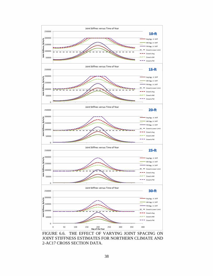
End of Life Joint Behavior

Avg Agg. Int.

AM Agg. Int.

PM Agg. Int.

Dowels Lower

Limit

Dowels Avg

Dowels AM

Dowels PM

FIGURE 6.5. ESTIMATES OF JOINT STIFFNESS VERSUS TIME OF YEAR FOR DOWELED AND AGGREGATE INTERLOCK CONTRACTION JOINTS FROM THE COMPREHENSIVE JOINT BEHAVIOR MODEL

The comprehensive model reveals that joint stiffness behavior is perhaps most sensitive to the design joint spacing. Slab length controls the joint opening rate parameter, dO/dT. To demonstrate the joint spacing effect, figure 6.6 shows the results of varying slab length from 10

37

to 30 feet on aggregate interlock joint stiffness and using site 2-AC17 site design parameters. This plot simulates how aggregate interlock joints would behave in a cooler northern USA climate, as a function of slab length and assuming northern spring or fall typical construction temperatures. The model predicts that at a joint spacing of about 16 to 17 feet, the aggregate interlock and LT will drop to zero during cold weather for just a few days during the coldest part of the year. For a joint spacing of 30 feet, the aggregate interlock joints have an estimated zero stiffness and LT for about 165 of the cooler days, a much longer period.

38

0

50000

100000

150000

200000

250000

0 50 100 150 200 250 300 350 400


Day of the Year

Joint Stiffnes versus Time of Year

Avg Agg. Jt. Stiff

AM Agg. Jt. Stiff

PM Agg. Jt. Stiff

Dowels Lower Limit

Dowels Avg

Dowels AM

Dowels PM

0

50000

100000

150000

200000

250000

0 50 100 150 200 250 300 350 400


Day of the Year


Avg Agg. Jt. Stiff

AM Agg. Jt. Stiff

PM Agg. Jt. Stiff

Dowels Lower Limit

Dowels Avg

Dowels AM

Dowels PM

0

50000

100000

150000

200000

250000

0 50 100 150 200 250 300 350 400


Day of the Year


Avg Agg. Jt. Stiff

AM Agg. Jt. Stiff

PM Agg. Jt. Stiff

Dowels Lower Limit

Dowels Avg

Dowels AM

Dowels PM

0

50000

100000

150000

200000

250000

0 50 100 150 200 250 300 350 400


Day of the Year


Avg Agg. Jt. Stiff

AM Agg. Jt. Stiff

PM Agg. Jt. Stiff

Dowels Lower Limit

Dowels Avg

Dowels AM

Dowels PM

0

50000

100000

150000

200000

250000

0 50 100 150 200 250 300 350 400


Day of the Year


Avg Agg. Jt. Stiff

AM Agg. Jt. Stiff

PM Agg. Jt. Stiff

Dowels Lower Limit

Dowels Avg

Dowels AM

Dowels PM

FIGURE 6.6. THE EFFECT OF VARYING JOINT SPACING ON JOINT STIFFNESS ESTIMATES FOR NORTHERN CLIMATE AND 2-AC17 CROSS SECTION DATA.

39

CHAPTER 7. COMPARING TEST SITE DATA TO FINITE ELEMENT ANALYSES The data obtained from the field test sites and the resulting calibrated joint stiffness models have established the joint design input for FEM analyses. The calibrated joint stiffness input takes into account the effects of typical loss of support along slab edges, looseness of aggregate interlock, and dowels on overall joint stiffness. FEM models matching four of the test site FWD data sets were developed using the ILSL2 software. These calibrated FEM models were used to calculate Load Transfer, LT values for different loads and gear configurations. When using FEM models and simulating loads plus curling, it is the percentage stress reduction in the loaded slab caused by joint stiffness, as compared to a free-edge loading condition that is the key index of Load Transfer, LT. The percent stress reduction in the loaded slab must be directly obtained from the jointed FEM model loaded slab stresses as follows: % Reduction in Loaded Slab Free-Edge Stress, LT = [L(L+T) (free-edge, kJ=0) - L(L+T) (kJ >0)]/L(L+T) (free edge, kJ =0)] (13) The stress value L(L+T) is the calculated combined wheel load plus temperature curling (L+T) stress in the FEM model loaded slab for varying joint stiffness values. The edge stress values for kJ greater than zero are compared to the free edge stress values calculated for kJ = 0. Figure 7.1 shows FEM generated LT curves for a 210-kip B747 gear simulation in the calibrated DIA FEM model, compared to a 40-kip FWD load simulation. The most critical LT curves are for the simulated downward slab curling. Wheel loads and curling both cause combining tension at the bottom of slab edge beneath the wheel load during downward curling. The LT value is lowest and bottom-of-slab edge stress is highest when slabs are curled downwards, when the top of the slab is significantly warmer than the bottom.

-20

-10

0

10

20

30

40

50

60

1000 10000 100000 1000000

LT, %


Flat LT-40 kip Single

up-curl Loaded Slab % Reduction 40-kip

down-curl Loaded Slab % Reduction 40-kip

Flat B747 4-wheel

Curled up B747 4-wheel

Curled down B747 4-wheel

40-kip Single FWD Load, versus B747 4-Wheel GearDIA FEM Model, k=250 pci, +/- 2 DegF/in Gradients

25%

FIGURE 7.1. COMPARISON OF LT CURVES FOR FWD LOADS AND B747 4-WHEEL GEAR LOADS SHOWING HOW LARGER LOADS/GEARS ACHIEVE HIGHER LT THAN SMALL CONCENTRATED SINGLE LOADS

40

7.1 ANALYSIS OF CURLING AND WARPING EFFECTS This section describes how to match the slab curvature changes measured in the field along with the FWD-based joint stiffness versus LTE data, to FEM model responses estimated for curling. The process is demonstrated using the data from site 5-AGG18. This test site showed the largest curling related variation of joint load transfer efficiency of all airfield pavement test sites. Figure 7.2 shows the computed joint stiffness versus LTE data along with the FEM model estimated characteristic joint stiffness curves for 0, 1, 2, and 3 F/in upward curling (morning) thermal gradients. The flat slab FEM curve hugs the lower boundary of the FWD data set, and increasing upward curling explains the observed changes in the joint stiffness responses at the site. Based on the range of measured response at the site, the apparent joint support changes caused by curling are equal to the effects calculated for a 1.5 to 1.8 F/in thermal gradient change in the FEM model. The variation appears to be closer to 1.5 F/in for higher stiffness values and closer to 1.8 F/in for lower stiffness values. This procedure provides a method for back-calculating apparent thermal gradients at a site as viewed through joint response data.

0%

10%

20%

30%

40%

50%

60%

70%

80%

90%

100%

0 50000 100000 150000 200000 250000 300000

LTE

-del

ta


Site 5-AGG18 Curling Simulation

Early AM

Late AM

Early PM

ILSL2 Flat

1degF/in

2degF/in

3degF/in

ILSL2 k = 450 psi/in

FIGURE 7.2. COMPARISON OF FWD JOINT STIFFNESS VERSUS LTE DATA, TO FEM MODEL CURLING SIMULATIONS FOR THE CALIBRATED ILSL2 FEM MODEL FOR SITE 5-AGG18

The measured slab curvature data are now compared to the FEM model predicted slab curvature in figure 7.3. The slab end slope sampling was applied to the FEM model slab shapes to obtain average slab curvature values for different thermal gradients. Pavement surface temperature ranged between about 80 and 130 F during testing at site 5-AGG18. For the measured curling curvature change of 0.00011 ft-1, the FEM model predicts that a linear thermal gradient of about 2.1 F/in would be required to develop this magnitude of curvature. The computed joint stiffness

41

response trends in figure 7.2 imply an effective thermal gradient effect on edge support of about 1.5 to 1.8 F/in thermal gradient range. Site 5-AGG18 apparently had the least compliant foundation for curling deformations of all test sites. A relatively high percentage of the measured thermal gradient curling could be identified in the joint response data. Some sites experienced very little apparent change in slab edge support while at the same time experiencing significant slab curvature changes from curling. These sites have softer and more compliant foundations. An ideal compliant foundation would allow curling to occur without having significant change in slab edge support. Softer foundations allow curling deflections to occur without offering as much bending restraint to slabs. The slab self weight sinking is greater for softer foundations and there is less of a chance of slab edge gap formation during upward curling or warping for softer foundations. Test site 2-AC17, overlying relative weak clayey subgrade, exhibited almost no change in FWD slab edge support response, while experiencing almost the same amount of measured curling slab shape change as site 5-AGG18. The subgrade at this site was very compliant, to the point where the edge support appears to remain very close to that of a “flat slab” even during relatively large slab curvature change.

0

0.00002

0.00004

0.00006

0.00008

0.0001

0.00012

0.00014

0.00016

0.00018

0 0.5 1 1.5 2 2.5 3 3.5

Average

Slab Curvature, ft

‐1

FEM Model Thermal Grad., degF/in

Curl = Measured Shape Change

Joint Response‐Least Compliant

Most Compliant

Warp = 8 AM Average

FIGURE 7.3. COMPARISON OF DIPSTICK MEASURED SLAB CURVATURE DATA TO FEM MODEL PREDICTED SLAB CURVATURE DATA FOR SITE 5-AGG18

7.2 COMPARISON OF ILSL2 TO FEAFAA The primary difference between the ILSL2 and FEAFAA FEM analysis software is the foundation idealizations used. FEAFAA incorporates a layered elastic half-space subgrade with elastic modulus, ES, while ILSL2 uses a dense-liquid subgrade representation. The FEAFAA software converts dense liquid modulus of subgrade reaction k-values (psi/in) to equivalent subgrade elastic modulus, ES, values (psi) using the following equation:

42

284.126 kES (14)

The FEAFAA simulations for this study assumed the base and subgrade layers to have the same elastic modulus. For dense liquid subgrade k-values of 200 psi/in and 430 psi/in, the converted elastic moduli are about 23,500 psi and 62,500 psi, respectively using this equation. ILLI-BACK was used for analysis of the FWD mid-panel load test data from the test sites. This software will backcalculate both dense-liquid and elastic-solid subgrade parameters. The backcalculation results from the test sites allow an independent check of the above equation. Figure 7.4 shows this comparison. Each data point represents an overall test site average based on hundreds of mid-panel load tests. Most of the test sites ended up significantly above the FAA equation trend line, with only one site (5-AGG18) being below. The best-fit power function for the full test site data, with similar form to the FAA equation, is provided. This relation represents apparent equivalencies for top-of-base foundation stiffness.

y = 380.22x0.8723

R² = 0.9159

0

20000

40000

60000

80000

100000

120000

140000

0 100 200 300 400 500 600 700 800

Elastic Solid

Modulus, Es, psi

Dense Liquid Modulus of Subgrade Reaction, k, psi/in

ILLIBACK Subgrade Parameter Comparison

Full Airfield Test Site Averages

FAA; Es = 26k^(1.284)

FIGURE 7.4. A COMPARISON OF THE k TO ES CONVERSION EQUATION FROM FEAFAA TO THE OVERALL TEST SITE AVERAGE TOP-OF-BASE SUPPORT VALUES OBTAINED USING ILLI-BACK

In order to compare FEAFAA to ILSL2, two-slab models having nearly identical cross sections were established in both software packages, simulating site 2-AC17. The characteristic joint stiffness curves generated from the two FEM analyses are shown in figure 7.5 overlying the computed joint stiffness data. The upper and lower limit subgrade k-values of 200 and 430 psi/in determined from Skarlatos/Ioannides-Edge and ILLI-BACK mid-panel analyses were used to develop the FEM curves. The FEAFAA generated joint stiffness curves do not match the measured trend as well as the ILSL2 curves. This is due primarily to the elastic solid subgrade model in FEAFAA. The best fit FEAFAA curve is approximately the k=200 psi/in equivalent (ES = 23,500 psi) curve.

43

Although not demonstrated here in this summary report, the FEAFAA software typically predicts lower LT values than ILSL2 for a given joint stiffness and pavement cross section. FEAFAA also predicts greater changes in LT from curling. LT curve shapes are similar for both procedures.

0%

10%

20%

30%

40%

50%

60%

70%

80%

90%

100%

0 50000 100000 150000 200000 250000 300000

LTE

-del

ta


Site 2-AC17

6:00-9:30 AM

9:45-11:30 AM

11:45-1:45 PM

ILSL2, k=200 flat

ILSL2, k=430 flat

FEAFAA, flat, k=200

FEAFAA, flat, k=430

LTE= 89%Possible Un-Cracked, 13%

FIGURE 7.5. COMPARISON OF CHARACTERISTIC JOINT STIFFNESS CURVES GENERATED USING FEAFAA AND ILSL2 FOR SITE 2-AC17

7.3 SUMMARY OF SLAB EDGE STRESS LT BEHAVIOR FROM FEM MODELS To demonstrate a typical range of LT values calculated from the FEM models for various load types and a range of thermal gradients, a summary LT versus joint stiffness plot for the DIA FEM simulations is provided in figure 7.6. Load simulations included:

40-kip FWD load used for matching to field measurements 200 psi contact pressure simulations at 30, 60 and 90 kips 90-kip two-wheel gear similar to a B737 gear 210-kip four-wheel gear similar to a B747 gear

The thermal gradients simulated (± 2 F/in) are relatively large and represent the outer boundaries of likely variation that will be observed at an airfield site. The 30-kip, 60-kip and 90-kip loads at 200 psi contact pressure demonstrate the effects of increasing load area size on LT values for single wheel loads. If the site subgrade is highly compliant to curl and warp, the joint LT values will stay near the flat slab zero gradient values (similar to site 2-AC17). If the subgrade is not compliant, LT values could vary about the flat slab values to some extent between the ranges shown (similar to site 5-AGG18). LT values are lowest for the downward curling simulations and for small area high contact pressure single wheel loads.

44

0

0.05

0.1

0.15

0.2

0.25

0.3

0.35

0.4

0.45

0.5

0 50000 100000 150000 200000 250000 300000

LT

Joint Stiffness (lb/in./in.)

Site DIA-CT18, Flat Analyses35-kip FWD, 12-in dia. 30-kip Single, 200 psi

60-kip Single, 200 psi 90-kip Single, 200 psi

B737- Dual B747- Tandem Duals

0

0.05

0.1

0.15

0.2

0.25

0.3

0.35

0.4

0.45

0.5

0 50000 100000 150000 200000 250000 300000

LT


Curled Down Analyses35-kip FWD, 12-in dia. 30-kip Single, 200 psi

60-kip Single, 200 psi 90-kip Single, 200 psi


0

0.05

0.1

0.15

0.2

0.25

0.3

0.35

0.4

0.45

0.5

0 50000 100000 150000 200000 250000 300000

LT


Curled Up Analyses

35-kip FWD, 12-in dia. 30-kip Single, 200 psi

60-kip Single, 200 psi 90-kip single, 200 psi


FIGURE 7.6. SUMMARY OF LT FUNCTIONS FOR VARIOUS LOAD TYPES FOR THE CALIBRATED ILSL2 FEM MODEL FOR SITE DIA-CT18 (k=250 psi/in, Ec=5,000,000 psi, Edge Length = 18.75 feet, ± 2 F/in gradients)

45

In chapter 5 it was demonstrated how joint stiffness varies as a function of average slab temperature. This previous discussion showed how LT varies as a function of joint stiffness for various load types using a calibrated FEM model. The site specific LT versus joint stiffness curves can be linked back to the site specific joint stiffness versus average slab temperature curves to establish a pavement design-specific set of LT versus average slab temperature curves for single-wheels, 2-wheel gears, and 4-wheel gears. If desired, climate models can be used to estimate a frequency distribution of slab temperature for a design year, and models from this study used to develop a frequency distribution of LT values for a given design year. If desired, the LT distribution can be transformed into a distribution of actual edge stress occurring over a given year for various loads and times of day. The combination of the closed form joint behavior models and the closed form LT prediction models allows the simulation of slab edge damage to be determined hour by hour if desired. These models were used to perform various sensitivity studies and develop recommendations regarding joint load transfer. 7.4 RECOMMENDED RANGES OF LT COEFFICIENTS FOR DESIGNS This section presents a discussion of how the research observations and models developed in this study can be integrated into an LT design scheme that is useful in the context of the current FAARFIELD single-slab FEM analysis, which does not use temperature gradient curling simulations. The effect of joint load transfer variations on pavement thickness design is highly dependent on the type of material damage model being used as the basis of thickness design calculations. The FAARFIELD single-slab FEM model rests a wheel or gear load on the slab edge and calculates a slab free edge stress for use in design. The traditional 25% edge stress reduction LT value is then applied to the free edge stress values for all load cases. These “75% of free edge stress” values are then entered into the current pavement damage model (Brill, 2010) and the damage caused by each load is estimated and accumulated. Slab thickness is adjusted until the accumulated damage is just less than 100 percent for the proposed amount and type of traffic at the facility. After reviewing the Version 6E damage model form, it was apparent that relative-damage functions could be generated from the damage model in a somewhat generic way for a wide range of loads. Four ratios of free edge stress to concrete modulus of rupture were used (3/7, 4/7, 5/7, and 6/7) and then a range of LT values were applied to the free-edge stresses. The number of passes to failure was determined for each simulated LT value and design stress/strength ratio and plotted as relative damage as shown in figure 7.7. The relative damage functions can be suitably reproduced using a series of fourth order polynomials. The coefficients for the four polynomials shown can be further parameterized as a series of third order polynomials. This nested polynomial parameterization allows a relative damage versus LT function to be determined for any free edge stress magnitude around the range of 0.4 to 0.9 times the concrete flexural strength and is considered suitable for use in design.

46

y = 348.1x4 ‐ 330.5x3 + 114.6x2 ‐ 17.39x + 0.996

y = 184.7x4 ‐ 193.3x3 + 76.70x2 ‐ 13.93x + 0.998

y = 93.62x4 ‐ 111.7x3 + 52.11x2 ‐ 11.42x + 0.999

y = 64.88x4 ‐ 79.70x3 + 40.11x2 ‐ 9.894x + 0.999

0

0.2

0.4

0.6

0.8

1

1.2

0 0.05 0.1 0.15 0.2 0.25 0.3 0.35 0.4

Relative

Damage, %

LT Value

Free‐Edge/MR = 3/7

Free‐edge/MR = 4/7



FIGURE 7.7. RELATIVE DAMAGE FUNCTIONS EXTRACTED FROM THE VERSION 6E PAVEMENT DAMAGE MODEL (FOR FLEXURAL STRENGTH = 700 PSI AND USING BASE AND SUBGRADE CONDITIONS SIMILAR TO THOSE USED FOR SITES DIA-CT18 AND 5-AGG18)

In general, each site will have a frequency distribution of LT values for each joint design that is primarily a function of the average slab temperature and also whether or not dowels or ties are used across the joints. As an example, consider an aggregate interlock joint in a cold northern climate that will have LT values ranging from 0.00 during winter to fully locked LT of 0.35 in the summer. As shown in figure 7.7, the amount of relative pavement damage occurring for each load during winter (LT near 0) is much greater than the damage occurring during summer when LT is near 0.35. If it is assumed that the frequency distribution of LT values over the year has a uniform distribution between 0.0 and 0.35, then the weighted LT value is the x-axis centroid for the relative damage function. Figure 7.8 presents the weighted LT functions calculated assuming a uniform distribution of LT values within the ranges shown. These lines can be used to approximate an overall effective annual LT value. The lowest line on the plot represents the weighted LT value that would be used for the example aggregate interlock joint when LT varies between 0.0 and 0.35 with a uniform distribution of LT values. The weighted LT value ranges from about 0.05 to 0.08 for increasing free edge stress magnitudes. For a doweled joint at the same site and having LT ranging from 0.20 to 0.35 from winter to summer, a weighted LT value of 0.23 to 0.25 would apply. The y-intercept values and slopes for this set of lines can be parameterized suitably into continuous functions using fourth order polynomials as shown in figure 7.9. Chapter 6 described how to estimate joint stiffness versus slab temperature for a given joint design. The first part of Chapter 7 described how convert joint stiffness data into LT values. Figures 7.8 and 7.9 show the most-simple form of the final answer to the fundamental question: What value of LT is appropriate for doweled versus tied versus aggregate interlock joints as a basis of design in FAARFIELD. This simple form requires an estimate of the winter and summer joint stiffness and LT values for a joint type and an assumption of uniform distribution

47

of LT values between winter and summer minimum and maximum values. This model is based on the current Version 6E pavement damage model. The weighted LT model in figure 7.9 can easily be programmed into a design routine. The line solutions for weighted LT are numerically stable and can be interpolated for any stress level between 0.0 and 1.0 times the flexural strength. However, the fourth-order polynomial representations for the relative damage curves in figure 7.7 become unstable for ratios of free-edge stress to concrete flexural strength values below 0.4. For ratio values less than 0.4, the curve for the 3/7 ratio should be used.

y = 0.071x + 0.014

y = 0.059x + 0.067

y = 0.032x + 0.131

y = 0.017x + 0.186

y = 0.038x + 0.211

y = 0.052x + 0.241

0

0.05

0.1

0.15

0.2

0.25

0.3

0.35

0 0.2 0.4 0.6 0.8 1

Weigh

ted LT Value

Free‐Edge Stress/Flexural Strength Ratio

0 to 0.35

0.05 to 0.35

0.1 to 0.35

0.15 to 0.35

0.2 to 0.35

0.25 to 0.35

Winter to Summer Joint LT Range

FIGURE 7.8. THE SIMPLIFIED WEIGHTED LT VALUES

48

y = ‐235.6667x4 + 125.9148x3 ‐ 18.8214x2 + 0.4431x + 0.0714

0

0.01

0.02

0.03

0.04

0.05

0.06

0.07

0.08

0 0.05 0.1 0.15 0.2 0.25 0.3

Winter Coolest Day LT Value

LT Slope

y = 183.3333x4 ‐ 98.6444x3 + 14.7583x2 + 0.5201x + 0.0144

0

0.05

0.1

0.15

0.2

0.25

0.3

0 0.05 0.1 0.15 0.2 0.25 0.3

Winter Coolest Day LT Value

LT Intercept

FIGURE 7.9. WEIGHTED LT INTERCEPT AND SLOPE VALUES TO BE USED TO PREDICT THE WEIGHTED LT VALUES

Figure 7.10 links the FEM generated LT curves to the comprehensive joint behavior model to predict LT as a function of average slab temperature for the DIA pavement design. The corresponding LTE and joint stiffness versus temperature trends were shown in figure 6.4. These plots can be used as a guide to estimate the winter LT values for a given site for thicker airfield pavements having joint spacing between about 16 and 22 feet and construction temperatures similar to those at the DIA instrumented test site. The plots show the new and projected older joint LT conditions for doweled and aggregate interlock joints. This plot reveals a key finding. The LT versus average slab temperature prediction is a nearly linear trend for the aggregate interlock component of total joint stiffness. LT versus slab temperature can be suitably approximated using a line between the TLock and TRelease temperatures, with LT = 0.0 at release and LT equal to the upper limit value associated with the upper limit joint stiffness for a given pavement cross section and load configuration at the TLock temperature (probably between 0.3 and 0.35). In general, the joint stiffness versus average slab temperature trends have significant upward curvature, while the LT versus joint stiffness trends have significant downward curvature. When these two relations are combined, the LT versus average slab temperature trend that results is nearly linear for aggregate interlock.

49

0

0.05

0.1

0.15

0.2

0.25

0.3

0.35

0.4

0 20 40 60 80 100 120

LT Factor

Average Slab Temperature, degF

Predicted LT vs. Temperature (New Joints)

AGG: 60‐k Single

AGG: 2 wheel gear

AGG: 4 wheel gear

DOWELS: 60‐k Single

DOWELS: 2 wheel gear


0

0.05

0.1

0.15

0.2

0.25

0.3

0.35

0.4

0 20 40 60 80 100 120

LT Factor

Average Slab Temperature, degF

Predicted LT vs. Temperature (Old Joints)

AGG: 60‐k Single

AGG: 2 wheel gear

AGG: 4 wheel gear

DOWELS: 60‐k Single



FIGURE 7.10. PLOTS TO BE USED FOR PREDICTING THE WINTER LT VALUES, GENERATED BY COMBINING THE FEM LT CURVES AND THE COMPREHENSIVE JOINT BEHAVIOR MODEL

7.5 BEST ESTIMATE OF LT The following example demonstrates how to combine all of the analytical procedures developed from this study to obtain the best possible estimate of weighted LT for a given pavement design and load scenario. Figure 7.11 shows measured average slab temperature data from DIA along with predicted temperatures from the integrated climate model (Rufino, Roesler and Barenberg 2004). The detailed LT prediction process uses this type of site temperature data and includes the following steps:

50

1. Establish an estimated frequency distribution of the average slab temperature data for a

given year for the design site as shown in figure 7.12. Average slab temperatures will vary less than average air temperatures.

2. Use the comprehensive joint stiffness behavior model from Chapter 6 to convert the x-axis temperature data from figure 7.12 into joint stiffness values as shown in figure 7.13. Figure 7.13 provides the frequency distribution of average joint stiffness values for a year for the various joint designs being used at the DIA site.

3. Use the FEM generated LT versus joint stiffness functions to convert the x-axis joint stiffness values into LT values for various wheel loads and gears, as shown in figure 7.14 for a B737 gear assembly.

4. Multiply the LT frequency distribution by the relative damage weighting function from figure 7.7 to obtain the damage weighted LT frequency distributions for the different joint designs as shown in figure 7.15.

5. Establish the weighted LT function’s x-axis centroid values. These values are the best guess single weighted annual LT values considering the best estimates of slab temperature variation at a site.

This example assumed a compliant softer subgrade and used the flat slab LT curves and did not simulate curling variations in LT. This is the type of “average-daily-value” analysis that would be used, for example, when annual temperatures are being accounted for, while curling variations are not being accounted for. This is the type of LT estimation process that is considered most appropriate for use with the current FAARFIELD single slab model framework that does not simulate curling variations.

FIGURE 7.11. DIA AIRPORT MEASURED VERSUS PREDICTED AVERAGE SLAB TEMPERATURE DATA FROM RUFINO, ROESLER AND BARENBERG, 2004

51

0

10

20

30

40

50

60

70

80

90

100

0 20 40 60 80 100 120

Percent, or Days per Year

Average Slab Temperature, degrees F

DIA Climate Data

Cumulative Dist. (Rufino et al 2004)

1‐Year Frequency Dist. Of Avg. Temp. (5‐degree ranges)

FIGURE 7.12. THE ANNUAL FREQUENCY DISTRIBUTION OF AVERAGE SLAB TEMPERATURE FOR THE DIA SITE

0

10

20

30

40

50

60

70

80

90

100

0 50000 100000 150000 200000 250000

Days per Year

Average Joint Stiffness, lb/in/in

DIA Joint Stiffness Yearly Distributions

Agg Interlock Joints

Doweled Joints

FIGURE 7.13. ANNUAL FREQUENCY DISTRIBUTIONS OF JOINT STIFFNESS AT DIA

52

0

10

20

30

40

50

60

70

80

90

100

0 0.05 0.1 0.15 0.2 0.25 0.3 0.35 0.4

Days per Year

B737 Gear LT Values

DIA Joint LT Yearly Distributions


Doweled Joints

FIGURE 7.14. THE FREQUENCY DISTRIBUTION OF LT VALUES AT DIA

0

2

4

6

8

10

12

14

16

18

20

0 0.05 0.1 0.15 0.2 0.25 0.3 0.35 0.4

Weighted Count per Year

B737 Gear LT Values

DIA Damage‐Weighted LT for a Year


Doweled Joints

0.110.32

FIGURE 7.15. DAMAGE-WEIGHTED LT FREQUENCY DISTRIBUTIONS AT DIA AND OVERALL WEIGHTED LT VALUES

Comparing the results in figure 7.15 to the simplified weighted LT values in figure 7.8 reveals similar results. If one were to select the simplified trend for DIA for aggregate interlock joints having winter to summer LT range of 0.05 to 0.35, which generally matches the actual LT frequency distribution range as shown in figure 7.14, the predicted weighted LT values would be about 0.09 to 0.12, as compared to 0.11 obtained using an actual temperature frequency

53

distribution estimate. This comparison should give confidence in using the simplified winter to summer LT range (figure 7.8) as the basis of design. As can be observed, the relatively accurate frequency distribution for LT values is not a uniform distribution. Because of the nature of the damage function, these weighted LT value trends are dominated by how the pavement system will behave in cooler weather. As shown in figure 7.12, the frequency distribution of temperatures has two primary peaks and these peaks represent the typical winter and summer equilibrium conditions at a site (solstices). Spring and fall are times of maximum rates of change and there are fewer days per year in these intermediate temperature ranges. Slab temperature frequency distributions for Denver, Colorado are dominated more by the winter equilibrium conditions as a result of being situated well north of the equator. As demonstrated, it is difficult to predict the winter LT value for a given design site. The winter LT prediction is perhaps most sensitive to the joint spacing selected for design. Figure 7.16 provides a guide for estimating the effective thermal range for the aggregate interlock component of a joint design and as a function of slab length. The upper plot provides a relatively accurate prediction of the temperature range from TLock to TRelease. This upper plot was obtained from the DIA-calibrated comprehensive joint behavior model. The lower plot uses the temperature range data to estimate the site average TRelease temperature for the aggregate interlock component of joint stiffness, plotted for varying average slab temperatures present during the few days after construction. The lower plot arbitrarily assumed the TLock temperature would be about 20 F higher than the average slab temperature present during the few days after construction. The values in the plots are representative of newer joint conditions. Aging will reduce the aggregate interlock thermal range and increase the release temperatures. Changing from a 25-ft joint spacing to a 20-ft joint spacing is estimated to lower the TRelease temperature for aggregate interlock by about 20 F. To estimate if the winter LT will be zero for aggregate interlock at a site, compare the estimated release temperature for the proposed joint spacing and slab early life temperatures to the typical average winter temperatures at the site.

54

y = 2429.6x‐1.187

0

20

40

60

80

100

120

140

0 10 20 30 40 50

Agg. Interlock Therm

al Range, degF

Slab Length, feet

‐100

‐80

‐60

‐40

‐20

0

20

40

60

80

100

0 10 20 30 40 50

Agg. Interlock Release Temp., degF

Slab Length, feet

45

55

65

75

85

95

FirstWeek Average

Slab Temperature

FIGURE 7.16. THE SENSITIVITY OF MEASURED DIA AGGREGATE INTERLOCK THERMAL RANGE (TLock – TRelease) TO SLAB LENGTH AND EARLY LIFE AVERAGE SLAB TEMPERATURES AFTER PLACEMENT

Addition of dowel and tie bars can keep LT values high during the winter. Testing of doweled joints has revealed that the modulus of dowel-concrete interaction can deteriorate significantly over time and from repeated traffic. Doweled joints must be properly designed considering dowel-to-concrete bearing stresses and loads on individual dowels. If the dowel-concrete interaction support zone is over-stressed dowels will lose support more rapidly over time. This study used the typical FAA doweled joint stiffness equation and performed backcalculations of apparent modulus of dowel-concrete interaction factors for doweled joint designs. In general, use the FAA doweled joint stiffness equation along with the following recommendations to develop joint stiffness estimates for doweled joint designs:

Limit the assumed modulus of dowel-concrete interaction for new joints to 5,000,000 psi/in.

55

The average modulus of dowel-concrete interaction during the service life will likely be about 3,000,000 psi/in.

In heavy traffic areas the modulus of dowel-concrete interaction will likely drop to levels below 1,000,000 psi/in near the end of the service life.

Set the D/s dowel component of joint stiffness determined from the FAA doweled joint stiffness equation to be just less than the recommended upper limit total joint stiffness values for locked joints shown in figure 6.3 for a given design slab thickness.

Aggregate interlock can be assumed to be present and vary with temperature in doweled contraction joints.

Construction joints were perhaps the most variable and least predictable type of joint. Aggregate interlock friction available on smoother construction joint faces is generally less than available on rougher cracked contraction joint faces. In addition, given the more complex construction process for a construction joint, it appears that dowel stiffness is generally reduced for construction joints as compared to cast-in dowel assemblies used for contraction joints. Further study is needed to better quantify construction joint stiffness and LT versus contraction joint stiffness and LT. In general aggregate interlock should be ignored for flat-faced construction joint designs and all joint resistance attributed to the dowel bars or tie-bars. As an interim guide until better data is available, the modulus of dowel concrete interaction factors recommended above for doweled contraction joints should be multiplied by 75% for use with doweled construction joint designs. In general, it will likely be either the plain aggregate interlock joints or the doweled construction joints that will be the weakest joints with lowest load transfer ability at an airfield test site. Tied contraction joints are generally designed to remain closed retaining nearly full aggregate interlock. The joint stiffness and corresponding LT values for new working joints shown in figure 6.3 can be assumed to be present at all times of the year for tied joints. However, a line of tied joints may cause greater joint openings to develop for joint lines adjacent to the tied joint lines. Excessive amounts of tied joints can result in slab cracking. Tied joints must be used with care and in strategic locations. Doweled and/or aggregate interlock joints are needed to allow and control thermal expansion and contraction and joint opening sizes. Random cracks will likely behave similar to aggregate interlock joints but possibly with poor spalling performance as the pavement ages.

56

CHAPTER 8. SUMMARY AND CONCLUSIONS This research project set out to address a long list of key questions regarding concrete airfield pavement joint load transfer behavior and history. This list of questions was presented in the beginning of this report and is now revisited. Brief summary answers are provided below for each question.

What is the genesis of the assumption that a partial load transfer of the load at a joint reduces flexural stress by 25%?

Answer: Detailed pavement analysis began to be used in the early and mid 1990s as a result of rapidly increasing demand for aircraft and increasing sizes of aircraft, WWII and other factors. The first tools to arrive for pavement slab analysis could not consider multiple slabs with joint effects in mathematical simulations. Only free-edge stress prediction equations were available (Westergaard, 1926). The 25% factor was a result of extensive research studies designed to calibrate the available free-edge stress model by Westergaard to field measurements of bending strain at real pavement joints. It was recognized early that LT was a dynamic stochastic variable and would vary considerably. The 25% factor is a design allowance factor and is not to be considered a real value present at all times in the field.

What were the variables examined that resulted in the adoption of the 25% value?

Answer: Test sites were established and strain gages installed in slab edges adjacent to joints. The test sites had varying slab thickness and foundation materials. Various load sizes and different types of joints were evaluated.

What variables used in the development of the current 25% assumption are valid and applicable to pavement design as it exists today?

Answer: All of the variables originally reviewed are still applicable today.

How sensitive are the pavement thickness design protocols being used to the assumed load transfer variables?

Answer: The sensitivity is closely related to the pavement damage model used for thickness design calculations. One way to view this sensitivity is through the relative damage functions provided in figure 7.7. For example, for LT values of 0.25 and 0.20, the relative damage factors are about 0.02 and 0.05, respectively. This means that less than 40 percent of the allowable traffic would be available for a design using 0.2 as the LT factor compared to an LT factor of 0.25.

Do the minimum design requirements dictate the thickness requirement?

Answer: When using the current FAA pavement damage model, the selection of the load transfer coefficient will dictate the required design thickness.

Is it feasible to dictate the use of a “short duration” period of low load transfer for the design?

Answer: It does appear feasible to develop such a design scheme. However, this research has shown that the LT factor for aggregate interlock joints will vary with a

57

nearly linear trend with respect to slab temperature. LT values will range from zero (for open joints) to about 0.35 (for joints tightly closed). For sites having longer slab lengths greater than 20 feet, it may be necessary to assign a short duration period of zero LT for aggregate interlock joints during the colder portions of winter in cold northern climates, as demonstrated in figure 6.6. For properly designed doweled and tied joints it does not appear necessary to use a period of low load transfer. The concept of the damage weighted annual effective LT is a better way of addressing seasonal variations in LT.

Under what conditions is there a difference in load transfer efficiency for a doweled, tied, and plain contraction joint?

Answer: The primary condition for which there are significant differences is cold weather when slabs contract and joint openings become large. The three joint types above all have fundamentally different behaviors. Tied joints are designed to remain tightly closed retaining high aggregate interlock stiffness and high LT during cold weather. In a properly designed tied joint, load transfer is mobilized primarily through aggregate interlock. LT values will remain high for tied joints during all slab temperatures provided the tie steel does not yield or break. Doweled joints are designed to open and close, and during winter all load transfer will be through the dowels. Dowel effectiveness will be dependent on how well the dowels are supported in the slabs. Aggregate interlock joints can completely lose all load transfer ability during cold weather.

On a contraction joint, does the depth of saw cut impact the value of load transfer efficiency?

Answer: Although this was not directly studied, it is clear that the answer is yes. The amount of aggregate interlock joint stiffness available will depend on the amount of joint crack face area that develops shear contact during joint deflections. However, it is more important to provide adequate saw cut depth to promote cracking of fresh concrete at the desired joint locations. Deeper saw cuts will result in less aggregate interlock joint stiffness being available and will also result in higher load related shear stresses on the aggregate interlock surfaces that do remain after saw cutting.

Is there an ambient environment regime where load transfer efficiency is nearly constant?

Answer: There are two ambient temperature regimes where joint stiffness and load transfer are nearly constant, very cold temperatures (joints fully open) and very hot temperatures (joints fully closed). When joints become fully closed, the upper limit joint stiffness trend lines provided in figure 6.3 should be considered to be present for all temperatures above the joint lock-up temperature.

Is there an ambient temperature environment when load transfer efficiency has a minimum value?

Answer: Yes it is during very cold weather. When joints become fully open during cold weather, aggregate interlock joints will have a constant zero LT value for longer slab lengths and higher paving temperatures (see figures 6.6 and 7.10). Doweled joints can also lose all aggregate interlock during cold weather and the load transfer will be constant and related to the dowel support quality.

58

Can ambient environment be a design variable? If so, what are the conditions that must be satisfied before a reasonable value for load transfer can be assigned?

Answer: Yes, ambient temperatures expected at a design site should be a design consideration. This research has shown that slab temperature is one of the most important parameters regarding load transfer. The calibrated joint stiffness versus slab temperature models and the FEM LT versus joint stiffness curves developed for this study were necessary in order to be able to obtain reasonable estimates for load transfer coefficients for designs as a function of ambient temperature variations.

What are the variables that affect the quantitative value of load transfer efficiency and are those variables equally significant?

Answer: Perhaps the most significant factor affecting load transfer is the choice of whether or not to use load transfer devices. If the design site will experience cold weather with temperatures well below the concrete casting temperatures, joint openings will likely be large during cold weather. If joint openings are expected to be large at a site (i.e., very cold winters), then load transfer devices are more desired. The two most important variables are slab length and ambient temperature variations and these appear to be roughly equally significant. These variables are followed by factors such as the concrete coefficient of thermal expansion. A high thermal expansion coefficient indicates a greater chance of larger joint openings during cold weather. Downward slab curling can cause an increase in load-related slab edge stress while at the same time causing a decrease in the LT factor.

If not equally significant, what variables can be ignored for the purpose of assigning a value for load transfer?

Answer: This study revealed that base type has relatively small effect on load transfer and may be ignored. There is some evidence that joints over cement treated bases may experience larger slab edge gaps during upward curling.

Is there a simple technique that can be employed to determine when aircraft gear configuration will significantly influence the quantitative value of load transfer efficiency?

Answer: Yes. Although it was not demonstrated in this summary report, the full report for this study provides regression formulae that can predict LT values for single wheel loads, two-wheel gears and four-wheel gears as a function of joint stiffness values for use in pavement analysis. Figure 7.6 demonstrates these curves showing how wheel load area size and gear type affected LT values.

Is there sensitivity in the thickness computation that is a result of the interaction between gear configuration, slab curling, slab warping, slab size and load transfer for a given set of variables?

Answer: Yes. Figure 7.6 demonstrates the sensitivity of LT to variations in joint stiffness and curling magnitudes for the DIA pavement design. Figure 8.1 shows a simplified example that demonstrates the thickness design sensitivity to the LT value assumed. For the example, free-edge stress values were calculated for a 60-kip 200 psi wheel load simulation for varying slab thickness values. Then various LT values were

59

applied to the free-edge stress values to develop the curves on the plot. For this example, assume the FAA pavement damage model indicates that the LT-adjusted edge stress must be limited to 450 psi for the 60-kip load in order to support the number of effective aircraft coverages proposed for the example design. If the traditional LT factor of 0.25 is applied to the free edge stress, the required slab thickness is about 15.1 inches. If the site design used all doweled joints with effective damage weighted LT values of 0.3, the required slab thickness would be about 14.6 inches. If the design were to use primarily aggregate interlock contraction joints and had a damage weighted LT value of about 0.05 (northern climate with cold winters and warm summer construction), the required slab thickness would be about 17.6 inches. Each type of gear at a design site will have a different value of effective limiting LT-adjusted edge stress that is related to the traffic mix and the number of coverages anticipated at the design site. Each type of gear will have a set of LT-adjusted stress curves as shown below.

200

250

300

350

400

450

500

550

600

650

700

14 16 18 20 22

LT‐Adjusted Edge

Stress, psi

Required Slab Thickness, in

60‐kip 200 psi Single Wheel

free edge

LT = 0.05

LT = 0.1

LT = 0.15

LT = 0.2

LT = 0.25

LT = 0.3

LT = 0.35

FIGURE 8.1. THE SENSITIVITY OF REQUIRED PAVEMENT SLAB THICKNESS VERSUS ASSUMED LT VALUE FOR THE EXAMPLE ALLOWABLE SLAB EDGE STRESS OF 450 PSI

What metric is best used to define and model joint load transfer when data are collected using a Falling Weight Deflectometer (FWD)?

Answer: The FWD device is designed to quantify slab deflections and therefore the deflection based load transfer efficiency (LTE) is the best index to obtain with the FWD device. Although not presented in this summary report, part of this research project included reviewing time history data for dynamic FWD joint load tests. Three different ways of calculating load transfer efficiency were evaluated: LTE calculated at the time of maximum load, LTE calculated at the time of maximum joint deflection difference, and LTE calculated using the maximum displacement values obtained from each FWD

60

sensor (the traditional method). It was determined that the best index is the LTE

determined with the traditional method using the maximum sensor displacements.

When using the FWD is it necessary to correct for slab bending?

Answer: Past research has proposed a bending correction factor for use with FWD joint load tests (Khazanovich and Gotliff, 2003). This bending correction factor adjusts the LTE measured from FWD deflections taken at 6-inches from the joint line to account for slab bending deflections occurring in the small zone on 6 inches on either side of the joint and between the FWD sensors. This past research has been primarily based on thinner roadway slab evaluations. Because airfield slabs are relatively thick and typically have relative dense edge subgrade support, it is not considered necessary to use this type of bending correction factor for thick heavy duty airfield pavement FWD evaluations. This slab bending correction is more important for thinner concrete slabs.

What dynamic loading is required to evaluate load transfer efficiency?

Answer: This is the one question on the list that remains relatively untested. A special load testing device would be needed to evaluate different loading rate effects on load transfer efficiency. The FWD device is a stationary dynamic load pulse type load test. This dynamic pulse can be considered to be somewhat like a rolling wheel load. When considering the typical load pulse duration for the FWD it is similar to the load pulse duration that would be generated by an aircraft wheel moving at about 40 mph. Therefore, it is safe to assume that the deflections measured using the FWD load test are smaller than deflections that would be measured for a static load test with the same load magnitude. In order to develop a longer duration load pulse, the FWD device would have to be modified to use a softer rubber buffer system for the FWD drop weight impact, along with a heavier drop weight. A device capable of using variable loading rates and heavy loads was not readily available for this study.

The researchers of the past studied load transfer and assigned the single 0.25 LT factor to all joints. Although the research behind this design allowance is sound, this 0.25 factor is clearly too large for aggregate interlock joints or for older worn doweled joints for pavement sites subject to cold weather. Table 8.1 provides what is considered to be revised overall average LT allowances for designs and considering the results and observations from this study. These are LT values expected for larger multi-wheel landing gears. It represents a step forward in understanding and away from past use of a global single value for all joint types. The table presents single representative LT design allowances for different joint types and broken down into three categories related to temperatures expected at the site. The category of Southern USA or Mild Climate is defined as sites where paving temperatures are likely to be below the average temperature for the pavement during the service life and joint openings will likely remain relatively small retaining significant aggregate interlock during most of the winter (Examples: California/Oregon Coast, Hawaii, Florida). The category of Middle USA Variable Climates is defined as sites where paving temperatures are likely to be about at or just below the average temperature for the pavement during service life and joint openings will vary more and be open larger during winter, but without fully opening and reaching a zero joint stiffness condition (North Carolina, Georgia and Tennessee). The category of Northern USA is defined as sites where paving temperatures are likely to be above the average temperature for the pavement

61

during service life and joint openings will likely be larger and more variable with joints having a zero joint stiffness condition during the winter (Minnesota, Michigan, and Wisconsin). As demonstrated in figure 7.15, the weighted LT values for aggregate interlock and doweled joints at DIA were 0.11 and 0.32, respectively. DIA would be right near the border of the Northern USA category.

TABLE 8.1. SIMPLIFIED LT VALUES CONSIDERING THERMAL EFFECTS AND JOINT TYPES

Southern USA or Middle USA NorthernJoint Type or Mild Climate Variable Climates USA

Aggregate Interlock Joint 0.2 0.15 0.1Doweled Contraction Joint 0.3 0.3 0.25

Doweled Construction Joint 0.25 0.25 0.2Fully Tied Joint 0.3 0.3 0.3

The magnitude of joint stiffness is the primary input variable for modern pavement FEM analyses that controls how much load is transferred from slab to slab and the overall load transfer, LT, value for a joint. In real pavement systems, the joint opening size, the roughness and stiffness of the crack face contact, and the amount and type of load transfer devices (dowels, tie bars) present across the joint control how load is transferred from slab to slab through the joint. During the literature review phase of the project, it was realized that there were no pre-existing methods for computing joint stiffness directly from joint deflection measurements. At the same time, it was realized that some way of directly calculating joint stiffness was required in order to accomplish the objectives of this research project. Therefore, considerable effort was put forth to develop a method for direct calculation of joint stiffness using non-destructive FWD data from joint load tests. This was the first major accomplishment of this study. The development of the new method for computing joint stiffness allowed new methods for back-calculating the modulus of subgrade reaction k-value along joint lines using the Skarlatos/Ioannides model or FEM models calibrated to match a site-specific LTE versus joint stiffness response. This was the second major accomplishment for this study. This accomplishment allowed a direct comparison of mid-slab support to slab edge support using the Slab Support Ratio concept. A detailed on-site non-destructive mechanistic evaluation procedure was developed for this study. The testing started typically before sunrise and extended to early afternoon and was designed to measure a site’s typical thermal curling response and how this curling affected joint load transfer. The evaluation procedure was performed thirteen times at eleven heavy duty airfield test sites. Data from additional test sites such as DIA, NAPTF, and LTPP GPS3 highway sites were also evaluated and used for this study. The establishment of the joint stiffness and FWD database was the third major accomplishment of this study. The field evaluations showed that the average Skarlatos-type Slab Support Ratio value was about 0.45 for typical in-service airfield pavements. Curling can cause apparent Slab Support Ratio to range from about 0.25 to 0.75 from morning to afternoon for sites experiencing large curling

62

shape change. Curling and warping trends measured at the airfield sites generally match trends previously measured at highway sites. Apparent slab edge loss of support and joint looseness were evaluated. Results showed that the magnitude of joint looseness that will develop near the end of service life can be assumed to be about 5 to 10 percent of the unloaded slab edge deflection magnitude for a typical 40-kip FWD load. The field evaluations allowed backcalculations of apparent modulus of dowel-concrete interaction values for in-service doweled joints. The overall average in-service modulus of dowel-concrete interaction was about 3,000,000 psi/in. The extensive joint behavior data were used to develop comprehensive joint stiffness prediction tools for jointed concrete pavements. The development of these tools was the fourth major accomplishment of this study. These models use the derivative concepts of dLTE/dT and dO/dT, along with the MDOT joint opening size prediction equation to develop a useful tool for predicting joint stiffness for aggregate interlock joints as a function of average slab temperature and pavement design parameters. For doweled joints, the stiffness prediction equation commonly used by FAA for joint designs is used to predict the component of joint stiffness added by load transfer devices. The joint stiffness models can demonstrate how joint stiffness will vary with slab temperature, by joint type, slab length and other parameters. The model can also simulate aging by reducing factors such as the modulus of dowel-concrete interaction for doweled joints, or by reducing dLTE/dO for the aggregate interlock component of joint stiffness. FEM pavement analysis software was calibrated to reproduce the measured joint responses. Using these calibrated FEM models, Load Transfer (LT) curves were developed for various wheel load sizes, 2-wheel gears and 4-wheel gears, as a function of joint stiffness and as a function of FEM model curling temperature gradients. The summary LT versus joint stiffness plots demonstrate the full range of LT values expected at commercial airfields. These LT versus joint stiffness curves can be combined with the joint stiffness versus temperature curves generated from the joint behavior model to obtain LT estimates as a function of average slab temperature for a design site. The FEM models are also used to show how slab curling affects joint behavior. The development of the calibrated FEM models and the FEM LT curves for various load sizes and gears was the fifth major accomplishment of this study. The pavement damage model contained within the FAA AC 150/5320 6E pavement thickness design model is combined with the joint stiffness versus temperature curves, and the LT versus joint stiffness curves to develop the concept of a “damage weighted LT value” for a given joint design at a site. Because of the nature of the pavement damage model and because LT values drop as joint opening size increases, the weighted LT value is dominated by how the joints will behave during cold weather. Simplified recommendations are provided for selecting a representative single value of LT for a given joint design. This was the underlying primary objective for this research project and represents the sixth major accomplishment of this study. In general, aggregate interlock joints having no load transfer devices will have a linear loss in LTE as a function of average slab temperature. In climates having a wide range of annual temperatures, and for long slabs, aggregate interlock joints will likely range from fully closed/locked during summer to fully open with zero LT during the coldest days of winter. As

63

slab lengths become shorter and winter slab temperatures warmer, the winter LT and joint stiffness values may be above zero. Adding load transfer devices will keep the winter LT values high provided the joints are properly designed. If the modulus of dowel-concrete interaction zone surrounding the dowel bars is over-stressed or becomes deteriorated, the dowels may become ineffective and the joint will lose load transfer ability over time, perhaps completely, such that the doweled joint behaves as an aggregate interlock joint. Tied joints using deformed steel essentially are designed to remain closed and keep aggregate interlock stiffness at levels more associated with summer joint opening sizes. A properly functioning tied joint develops total joint stiffness more from aggregate interlock than from the tie steel. The aggregate interlock component of construction joint smooth faces has smaller magnitude than naturally cracked faces. It is generally recommended that only the dowel component of total joint stiffness be used for construction joint designs. The detailed site evaluations reveal that it should be assumed that initial dowel-concrete interaction modulus values will be lower for construction joints, and that the dowel-concrete interaction modulus will deteriorate faster for construction joints. This study has clearly shown that smooth-face longitudinal doweled construction joints should use lower design joint stiffness and LT than transverse naturally cracked doweled joints across the paving lanes. Additional side-by-side comparisons, as demonstrated herein, will be required before these differences can be accurately quantified. Regarding joint design philosophy, it is recommended that the dowel component of total joint stiffness not be set too high. The dowel component of total joint stiffness should be designed to be less than the “locked” upper limit total joint stiffness values recommended from this study and presented in Chapter 6. There may be undesirable stress concentration effects around dowels if the dowel shear stiffness is significantly larger than the slab concrete shear stiffness. Based on this study, it is recommended that FWD evaluations for sites be focused on testing during the cooler periods of the year. However, wet frozen foundation conditions should be avoided. It should be attempted to occasionally obtain data below freezing but this data should be obtained in the fall season before the foundation becomes frozen solid. Testing during the warmer summer months will reveal more locked joints and reveal less critical information. Pavements built in cooler weather will generally have higher load transfer values than those built in warmer weather, but paving temperature is not necessarily a controllable design value. The relation between the paving temperatures, joint opening size, and the TLock and TRelease temperatures for aggregate interlock joints deserves additional future studies. Even if pure aggregate interlock joints are not being constructed much in the future, the aggregate interlock mechanism is still occurring with the doweled joints and should be studied independently. It will be easier to quantify this effect by evaluating pure aggregate interlock joints without having to attempt to mathematically separate out dowel effects. It is difficult to precisely determine how much of a total computed joint stiffness is from dowels versus aggregate interlock. In general, this study has demonstrated how a properly designed nondestructive mechanistic evaluation procedure can be used to quantify a site’s key mechanistic responses. These fundamental mechanistic responses are common to most joint-related pavement analysis

64

procedures and evaluation schemes. In this study, these mechanistic responses were compared specifically to the FAA airfield pavement design concepts; the LT value and the FAA AC 150/5320 6E pavement damage model. The result is a suitable solution of the Load Transfer, LT design problem in the context of the Version 6E damage model. Obtain the full report from this study for more details and analyses.

65

BIBLIOGRAPHY Advisory Circular AC 150/5320-6D (1995), with four official changes. Federal Aviation Administration. Advisory Circular AC 150/5320-6E (2010). Federal Aviation Administration. Ahlvin, R. G. (1991). “Origin of Developments for Structural Design of Pavements”, Technical Report GL-91-1, USAE Waterways Experiment Station, Vicksburg, MS. Ahlvin, R. G. et al. (1971). “Multiple-Wheel, Heavy Gear Load Pavement Tests”, Technical Report No. S-71-1, 5 volumes, USAE Waterways Experiment Station, Vicksburg, MS. Armaghani J.M., Lybas J.M., Tia M., Ruth B.E., (1986). “Concrete Pavement Joint Stiffness Evaluation”. Transportation Research Record 1099, TRB. Barenberg E. J. and R. E. Smith. (1979). “Longitudinal Joint Systems in Slip-Formed Rigid Pavements, Vol. I: Literature Survey and Field Inspection” Report No. FAA-RD-79-4-I, Federal Aviation Administration, Washington, D.C. Barenberg, E.J. Arntzen, D.M. (1981). “Design of Airport Pavement as Affected by Load Transfer and Support Conditions”. Proceedings of the Second International Conference on Concrete Pavements. Purdue University. Barker W.R. (1981). “Introduction to a Rigid Pavement Design Procedure”. Proceedings of the Second International Conference on Concrete Pavements. Purdue University. Bradbury, R.D. (1938). “Reinforced Concrete Pavements”, Wire Reinforcement Institute, Washington, DC. Brill, D.R. (1998). “Development of Advanced Computational Models for Airport Pavement Design”. DOT/FAA/AR-97/47. US DOT Office of Aviation Research. Brill, D.R. (2010). “Calibration of FAARFIELD Rigid Pavement Design Procedure”. DOT/FAA/AR-09/57. Office of Research and Technology Development, Washington, DC 20591. Bush III, A.J. Hall, J.W. (1981). “Experience with Nondestructive Structural Evaluation of Airport Pavements”. Proceedings of the Second International Conference on Concrete Pavements. Purdue University. Bush III, A.J., Alexander, D.R., Hall, J.W. (1985). “Nondestructive Airfield Rigid Pavement Evaluation”. Proceedings of the Third International Conference on Concrete Pavements. Purdue University.

66

Bush III, A.J., Brown, W.R., Bailey, C.E. (1989). “An Evaluation Procedure for Rigid Airfield Pavements”. Proceedings of the Fourth International Conference on Concrete Pavements. Purdue University. Byrum, C.R., Hansen W., Kohn S.D. (1997) “The Effects of Strength and Other Properties on the Performance of PCC Pavements”. Proceedings of the Sixth International Conference on Concrete Pavements Design and Materials for High Performance. Purdue University, Nov. 18-21, 1997. Byrum, C.R. (2009) “Measuring Curvature in Concrete Slabs and Connecting the Data to Slab Modeling Theory”. Transportation Research Record 2094, Transportation Research Board, National Academy Press, Washington DC. Byrum, C.R. (2000). “A High Speed Profiler Based Slab Curvature Index for Jointed Concrete Pavement Curling and Warping Analyses”. Ph.D. Dissertation, University of Michigan, 2001. Byrum, C.R. (2001). “The Effect of Locked-in Curvature on Pavement Performance”. Published in a book titled, “Long-Term Pavement Performance: Making Something of It”. Edited by R.G. Hicks and J. B. Sorenson. American Society of Civil Engineers, 2001. Crovetti, J.A. (1994). “Design and Evaluation of Jointed Concrete Pavement Systems Incorporating Open-Graded Permeable Bases”. PhD Dissertation, University of Illinois at Urbana-Champaign Department of Defense. (2001). “Pavement Design for Airfields” UFC 3-260-02, Washington, DC. Fine, Lenore and Remington (1972). “The US Army in WWII: The Corps of Engineers: Construction in the United States”, Office of the Chief of Military History, US Army, Washington, D.C. Finney, E., Oehler, L. (1959). “Final Report- Design Project Michigan Test Road”. Michigan State Highway Department Report No. 302, Project No 39 F-7(2). Gillespie, T. D. et al. (1993). “Effects of Heavy-Vehicle Characteristics on Pavement Response and Performance”. NCHRP Report 353, TRB National Research Council. Washington D. C. Grau, R. W. (1972). “Strengthening of Keyed Longitudinal Construction Joints in Rigid Pavements” Miscellaneous Paper S-72-43. US Army Engineer Waterways Experiment Station, Vicksburg, MS. Guo, H., Larson, R.M., Snyder, M.B. (1993). “A Non-Linear Mechanistic Model for Dowel Looseness in PCC Pavements”. Proceedings of the Fifth International Conference on Concrete Pavements. Purdue University. Hammons, M., D. Pittman, and D. Mathews. (1995). “Effectiveness of Load Transfer Devices”

67

DOT/FAA/AR-95/80, Federal Aviation Administration, Washington, D.C. Hammons, M. I (1998). “Advanced Pavement Design: Finite Element Modeling for Rigid Pavement Joints, Report II: Model Development”. DOT/FAA/AR-97/7. US DOT Office of Aviation Research. Hansen, W. et al. (1996). “The Effect of Higher Strength and Associated Concrete Properties on Pavement Performance (Interim Report)”. FHWA DTFH61-95-R-00108. Hutchinson, R. L. and P. Vedros (1977). “Performance of Heavy-Load Portland Cement Concrete (Rigid) Airfield Pavements” Proceedings of the 1st International Conference on Concrete Pavements, Purdue University, West Lafayette, IN. Hutchinson, R. L. (1966). “Basis for Rigid Pavement Design for Military Airfields”, Miscellaneous Paper No. 5-7, USAE Ohio River Division Laboratory, Cincinnati, OH. Ioannides, A. M. and M. I. Hammons. (1996). “Westergaard-Type Solution for Edge Load Transfer Problem” Transportation Research Record 1525, Transportation Research Board, Washington, D.C. Ioannides, A.M. and Khazanovich, L., "Nonlinear Temperature Effects on Multi-Layered Concrete Pavements," Journal of Transportation Engineering, ASCE, 124, 2, (Mar./Apr., 1998): 128-136. Jensen, E.A., Hansen, W. (2001). “Mechanism of Load Transfer Crack Width Relation in JPCP: Influence of Coarse Aggregate Properties”. Proceedings of the Seventh International Conference on Concrete Pavements. Purdue University. Jun, D.X., Ming, H.X., Jun, Z.J., (1997). “The Loss of Load Transfer Capacity at Joints of Airfield Concrete Pavements Under Repetitive Loads”. Proceedings of the Sixth International Conference on Concrete Pavements. Purdue University. Kawa, I. et al. (2002) “Implementation of Rigid Pavement Thickness Design for New Pavements” Proceedings of the 2002 Airport Technology Transfer Conference. Federal Aviation Administration. May, 2002. Kazuyuki, K., Nakagawa, S., Nishizawa, T., Kasahara, A. (1993). “Evaluation Method for Joint Load Transfer Efficiency in Concrete Pavements”. Proceedings of the Fifth International Conference on Concrete Pavements. Purdue University. Khazanovich L. Gotlif, A. (2003) “Evaluation of Joint and Crack Load Transfer- Final Report”. FHWA-RD-02-088. National Technical Information Services, 2003. Kohn, S.D. (1985). “Evaluation of the FAA Design Procedure for High Traffic Volume Rigid Pavements”. Proceedings of the Third International Conference on Concrete Pavements. Purdue University.

68

Kohn, S.D., Gemayel, C.A., Alexander, D.R. Tons, E. (1989). “Development of a Thickness Design Procedure for Stabilized Layers under Rigid Airfield Pavements”. Proceedings of the Fourth International Conference on Concrete Pavements. Purdue University. Marsey, W., Dong, M. (2004) “Profile Measurements of Portland Cement Concrete Test Slab at the National Airport Test Facility”. Proceedings of the 2004 FAA Worldwide Airport Technology Transfer Conference. Mellinger, F. and P. Carlton. (1955). “Application of Models to Design Studies of Concrete Airfield Pavements” Proceedings of the 34th Annual Meeting, Highway Research Board, Washington, D.C. Nishizawa, T., Koyanagawa, M., Takeuchi, Y., Kimura, M. (2001). “Study on Mechanical Behavior of Dowel Bar in Transverse Joint of Concrete Pavement”. Proceedings of the Seventh International Conference on Concrete Pavements. Purdue University. Nishizawa, T., Fukuda, T., Matsuno, S., (1989). “A Refined Model of Doweled Joints for Concrete Pavement using FEM Analysis”. Proceedings of the Fourth International Conference on Concrete Pavements. Purdue University. Nishizawa, T., Ozeki, T., Katoh, K., Matsui, K., (2009). “FEM Analysis of Thermal Stresses in Thick Airfield Concrete Slabs”. Proceedings of the 88th Annual Meeting of the Transportation Research Board, pre-print CD ROM. The National Academies. Owusu-Antwi, EB., Meyer, A.H., Hudson, W.R., (1989). “Preliminary Evaluation of Procedures for the Assessment of Load Transfer Across Joints and Cracks in Rigid Pavements using the Falling Weight Deflectometer”. Proceedings of the Fourth International Conference on Concrete Pavements. Purdue University. Parker Jr., F., Barker, W., Gunkel, R., Odom, E. (1979) Development of a Structural Design Procedure for Rigid Airport Pavements. FAA-RD-77-81. U.S.D.O.T. 1979. Pringle, T. (1950). “Structural Design of Joints for Airport Pavements” American Concrete Institute Title No. 46-59 Prozzi, J., Balmaceda, P., De Beer, M. (1993). “Nondestructive Tests Procedure for Field Evaluation of Transverse Joints in Concrete Pavements”. Proceedings of the Fifth International Conference on Concrete Pavements. Purdue University. Ricalde, L (2007). Analysis of HWD Data from CC2 Traffic Tests at the National Airport Pavement Test Facility. Proceedings of the 2007 FAA Worldwide Airport Technology Transfer Conference.

69

Roesler, J.R., Hiller, J.E., Littleton, P.C. (2005). “Large Scale Airfield Concrete Slab Fatigue Tests”. Proceedings of the Eighth International Conference on Concrete Pavements. Purdue University. Roesler, J., Evangelista, F., Domingues, M. (2007). “Effect of gear positions on airfield rigid pavement critical stress locations”. Proceedings of the 2007 FAA Worldwide Airport Technology Transfer Conference. Atlantic City, NJ. 2007. Rollings, R. S. (2003). “Evolution of Airfield Design Philosophies” Proceedings, XXII World Road Congress, Permanent International Association of Road Congresses, Durban, South Africa. Rollings, R. S. (2001). “Concrete Pavement Design: Its More than a Thickness Design Chart” Proceedings, 7th International Conference on Concrete Pavements, Orlando, Florida. Rollings, R. S. and D. W. Pittman. (1992). "Application of Field Instrumentation and Performance Monitoring of Rigid Pavements,"ASCE Journal of Transportation Engineering, Vol. 118, No. 3. Rollings, R. S. and M. P. Rollings. (1991). “Pavement Failures: Oversights, Omissions, and Wishful Thinking,” ASCE Journal of Performance of Constructed Facilities, Vol. 5, No. 4. Rollings, R. S. (1987). “Design of Rigid Overlays for Airfield Pavements,” doctoral dissertation, University of Maryland, (UMI Dissertation Information Services, No. 8808598). Rollings, R. S. (1989). “Developments in the Corps of Engineers Rigid Airfield Pavement Design,” Proceedings, 4th International Conference on Concrete Pavements, Purdue University, West Lafayette, IN. Rollings, R. S. (1981). “Corps of Engineers Design Procedures for Rigid Airfield Pavements,” Proceedings, 2nd International Conference on Concrete Pavements, Purdue University, West Lafayette, IN. Rufino, D.M., Roesler, J. Berenberg, E., Tutumuler, E. (2001). “Analysis of Pavement Responses to Aircraft and Environmental Loading at Denver International Airport”. Proceedings of the Seventh International Conference on Concrete Pavements. Purdue University. Rufino, D.M. (2003). “Mechanistic Analysis of In-Service Airfield Concrete Pavement Responses”. PhD Dissertation, University of Illinois at Urbana-Champaign. Rufino, D.M., Roesler, J. Berenberg, E (2004). “Mechanistic Analysis of Pavement Responses From Denver International Airport”. FAA Center of Excellence for Airport Technology. C.O.E. Report No. 26. Rufino, D., Roesler, J. (2004) “Effect of pavement temperature on concrete pavement joint responses” Proceedings of the 2004 FAA Worldwide Airport Technology Transfer Conference. Atlantic City, NJ. 2004.

70

Sale, J.P. (1977). “Rigid Pavement Design for Airfields”. Proceedings of the First International Conference on Concrete Pavements. Purdue University. Sale, J. P. and R. L. Hutchinson. (1959). “Design of Rigid Pavement Design Criteria for Military Airfields” Journal of the Air Transport Division, Vol. 85, No. 3, ASCE. Skarlatos, M.S. and Ioannides A.M. (1998). "The Theory of Concrete Pavement Joints" Proceedings, Fourth International Workshop on design theories and their verification of concrete slabs for pavements and railroads, 10-11 September, Bussaco, Portugal, pp. 187-208. Skarlatos, M. S. (1949). “Deflections and Stresses in Concrete Pavements of Airfields with Continuous Elastic Joints” Report AD 628501, US Army Engineer Ohio River Division Laboratories. Strauss, P.J., Perrie, B.D., du Plessis, L., Rossmann, D. (2005). “Load Transfer through Aggregate Interlock: Crack Width, Aggregate Type, and Performance”. Proceedings of the Eighth International Conference on Concrete Pavements. Purdue University. Tabatabaie, A.M. et al (1979). “Longitudinal Joint Systems in Slip-Formed Rigid Pavements, Vol. II: Analysis of Load Transfer Systems for Concrete Pavements” Report No. FAA-RD-79-4-I, Federal Aviation Administration, Washington, D.C. Teller, L.W., Sutherland E.C. (1936). “The Structural Design of Concrete Pavements Part 2- Observed Effects of Variations in Temperature and Moisture on Size Shape and Stress Resistance of Concrete Pavements”. Public Roads Journal of Highway Research, USDA Vol 16., No. 9. Teller, L.W., Sutherland E.C. (1936). “The Structural Design of Concrete Pavements Part 3- A Study of Concrete Pavement Cross Sections”. Public Roads Journal of Highway Research, USDA Vol 16., No. 10. Teller, L.W., Sutherland E.C. (1936). “The Structural Design of Concrete Pavements Part 4- A Study of the Structural Action of Several Types of Transverse and Longitudinal Joint Designs”. Public Roads Journal of Highway Research, USDA Vol 17., No. 7 and No. 8 Teller, L.W., Cashell, H.D. (1958). “Performance of Dowelled Joints under Repetitive Loading”. Public Roads, Volume 30, No. 1. US Department of Commerce. US Army Corps of Engineers. (1950a). “Lockbourne No. 2 - Experimental Mat,” Rigid Pavement Laboratory. US Army Corps of Engineers. (1950b). “Lockbourne No. 2 - Modification, Multiple-Wheel Study,” Rigid Pavement Laboratory.

71

US Army Corps of Engineers. (1946). “Lockbourne No. 1 Test Track, Final Report,” Rigid Pavement Laboratory. Van Breemen, W., Finney, E. (1950). “Design and Construction of Joints in Concrete Pavements”. American Concrete Institute Title No. 46-59. Westergaard, H. M., (1948). “New Formulas for Stresses in Concrete Pavements of Airfields,” Transactions, ASCE, Vol. 113, pp. 425-444. Westergaard, H.M. (1927). “Analysis of Stresses in Concrete Roads Caused by Temperature”. Public Roads Journal of Highway Research, USDA Vol 8., No. 3. Westergaard, H.M. (1926). “Stresses in Concrete Pavements Computed by Theoretical Analysis”. Public Roads Journal of Highway Research, USDA, Vol. 7., No. 2. Zollinger, D.G., Soares, J. (1999) “Performance of Continuously Reinforced Concrete Pavements: Volume VII: Summary”. FHWA-RD-98-102. Federal Highway Administration.

Date post:	11-Feb-2022
Category:	Documents
Upload:	others
View:	2 times
Download:	0 times

summary report - The Innovative Pavement Research Foundation

Documents