32
Summer School on Multidimensional Poverty 8–19 July 2013 Institute for International Economic Policy (IIEP) George Washington University Washington, DC
| Date post: | 28-Dec-2015 |
| Category: |
Documents |
| Upload: | christopher-gibbs |
| View: | 214 times |
| Download: | 0 times |

Summer School on Multidimensional Poverty
8–19 July 2013
Institute for International Economic Policy (IIEP)George Washington University
Washington, DC

Changes in Bolivia, Ethiopia, Nepal and Uganda
30%
35%
40%
45%
50%
55%
60%
65%
70%
75%
80%
0% 10% 20% 30% 40% 50% 60% 70% 80% 90% 100% 110%
Ave
rage
Inte
nsity
of
Pove
rty
(A)
Percentage of People Considered Poor (H)
Poorest Countries, HighestMPI
The size of the bubbles is a proportional representation of the total number of MPI poor in each country
UgandaBolivia
Nepal
Ethiopia

How the best countries reduced MPI
-8.00
-7.00
-6.00
-5.00
-4.00
-3.00
-2.00
-1.00
0.00
Nepal(.350)
Bangladesh(.365)
Rwanda(.460)
Ann
ualiz
ed A
bsol
ute
Cha
nge
in p
ropo
rtio
n w
ho is
poo
r and
dep
rive
d in
...
Nutrition
Child MortalityYears of SchoolingAttendance
Cooking FuelSanitation
Water
Electricity
Floor
Assets

xi1 xi2 xi3 xi4 xi5 Ci(k>=2)
g0(k>=2): 0 0 0 0 0 00 0 0 0 0 00 0 0 0 0 01 1 1 0 1 41 0 0 1 0 2
CenH: 2/5 1/5 1/5 1/5 1/5
The AF method and two points in time
Time 2Time 1xi1 xi2 xi3 xi4 xi5 Ci(k>=2)
g0(k>=2): 0 0 0 0 0 00 0 0 0 0 00 1 1 0 0 21 1 1 0 1 41 1 1 1 1 5
CenH: 2/5 3/5 3/5 1/5 2/5
In this example we know how each individual have change over time, like in panel data, when using cross sectional data we do not have this level of detail.
H= 3/5A= 11/5 * 1/3 =11/15
M0 = 3/5 * 11/5 = 11/25
H= 2/5A= 6/5*1/2 = 6/10
M0 = 2/5 * 6/10 = 6/25

Annualized Absolute Change:
Annualized Relative Change:
ΔX=(Xt’-Xt)Absolute Change:
Relative Change: %ΔX=(Xt’-Xt)/Xt
ΔX=(Xt’-Xt)/(t’-t)
%ΔX=(Xt’-Xt)/Xt (t’-t)
Variation over time
If we would like to compare different
periods
Group decomposition of change in poverty
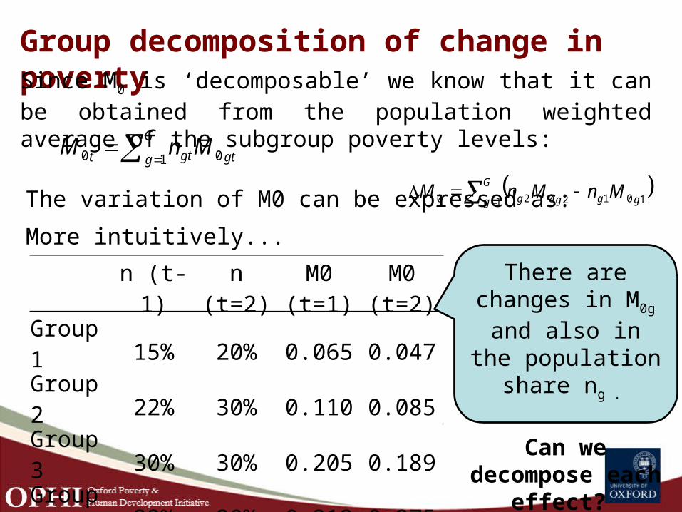
Group decomposition of change in poverty
The variation of M0 can be expressed as:
Since M0 is ‘decomposable’ we know that it can be obtained from the population weighted average of the subgroup poverty levels:
G
g gtgtt MnM1 00
G
g gggg MnMnM1 1012020
More intuitively...
n (t-1)n
(t=2)M0
(t=1)M0
(t=2)Group 1 15% 20% 0.065 0.047Group 2 22% 30% 0.110 0.085Group 3 30% 30% 0.205 0.189Group 4 33% 20% 0.312 0.275Total 100% 100% 0.198 0.147
There are changes in M0g and also in the
population share ng .
Can we decompose
each effect?
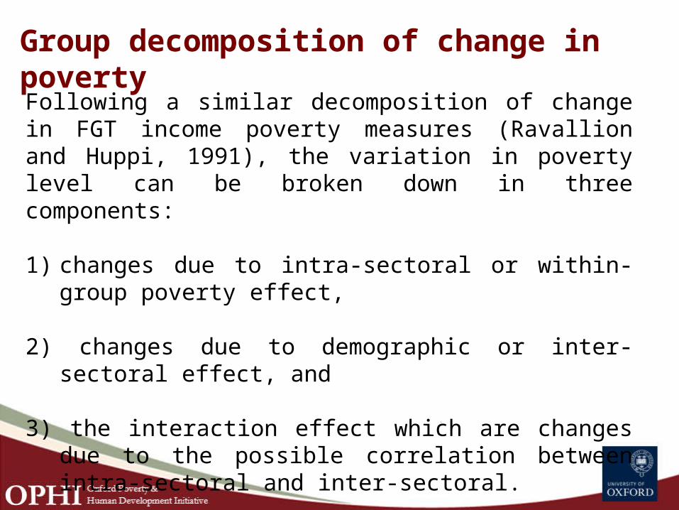
Group decomposition of change in poverty Following a similar decomposition of change in FGT income poverty measures (Ravallion and Huppi, 1991), the variation in poverty level can be broken down in three components:
1) changes due to intra-sectoral or within-group poverty effect,
2) changes due to demographic or inter-sectoral effect, and
3) the interaction effect which are changes due to the possible correlation between intra-sectoral and inter-sectoral.

Group decomposition of change in poverty
n2
n1
M02 M01
Δ n= n2-n1
Δ M0= M02-M01
So the overall change in the adjusted headcount between two periods t (1 and 2) can be express as follows:
G
g
G
g gggg
G
g gggggg nnMMnnMMMnM1 1 1210201 1210102010
Within-group poverty effect
Demographic or sectoral
effect
Interaction or error term
(within-group * demographic)
The interaction effect is difficult to interpret and
there is an arbitrariness in
the period of reference
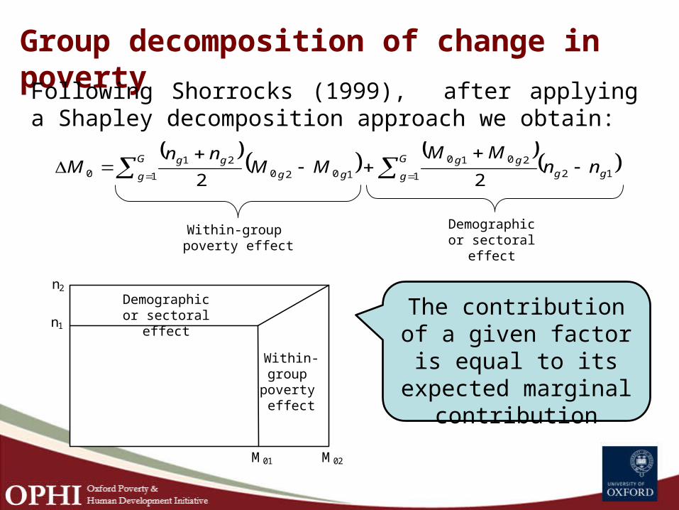
Group decomposition of change in poverty Following Shorrocks (1999), after applying a Shapley decomposition approach we obtain:
Within-group poverty effect
Demographic or sectoral
effect
The contribution of a given factor is
equal to its expected marginal
contribution
121
2010
1 102021
0 22 gg
G
g
ggG
g gg
gg nnMM
MMnn
M
n2
n1
M02 M01
Within-group
poverty effect
Demographic or sectoral
effect

Group decomposition of change in poverty
Within-group Effect
Demographic effect ΔM0
Group 1 2.7% 0.8% 3.5%Group 2 23.1% 8.5% 31.5%Group 3 34.3% -0.1% 34.1%Group 4 8.9% 0.5% 9.4%Group 5 23.8% -2.8% 21.0%Group 6 8.6% -8.2% 0.4%Overall Population 101.4% -1.4% 100%
Group 3 contributes the most to overall poverty reduction which is almost exclusively due to a within-group effect.
Group 2 contributes nearly as much as group 3 but part of the effect is due to reducing the population share.
Despite reducing poverty, group 6 had an almost cero overall effect because of an increase in population share
The marginal figures shows how much the overall within-group effect would have been if we extract the demographic effect

Decomposition by incidence and
intensity

14
-.030 -.025 -.020 -.015 -.010 -.005 .000 .005 .010
Annualized Absolute Variation in MPI-.030 -.020 -.010 .000 .010
NepalRwandaBangladeshGhanaTanzaniaCambodiaBoliviaUgandaEthiopia 1Ethiopia 2LesothoNigeriaKenyaMalawiZimbabweIndiaPeruColombiaSenegalGuyanaJordanArmeniaMadagascar
Annualized Absolute Variation in MPI-.030 -.020 -.010 .000 .010
NepalRwandaBangladeshGhanaTanzaniaCambodiaBoliviaUgandaEthiopia 1Ethiopia 2LesothoNigeriaKenyaMalawiZimbabweIndiaPeruColombiaSenegalGuyanaJordanArmeniaMadagascar
Annualized Absolute Variation in MPI
79%
68%
67%79%
21%
32%
33%21%
71%
74%85%
78%37%
45%83%
94%83%
60%79%
88%86%
90%
16%
95%
107%
29%
26%15%
22%
63%55%
17%
6%17%
40%
21%12%
14%10%
16%
Intensity and Incidence: both reduce MPI
68%45%
94%
32%55%
6%
Rwanda 2005-2010
Ethiopia 2005-2011
Nigeria 2003-2008
Incidence of poverty effect (H)Intensity of poverty effect (A)
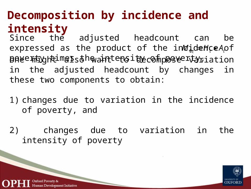
Decomposition by incidence and intensity Since the adjusted headcount can be expressed as the product of the incidence of poverty times the intensity of poverty, one might also want to decompose variation in the adjusted headcount by changes in these two components to obtain:
1) changes due to variation in the incidence of poverty, and
2) changes due to variation in the intensity of poverty
ttt AHM 0
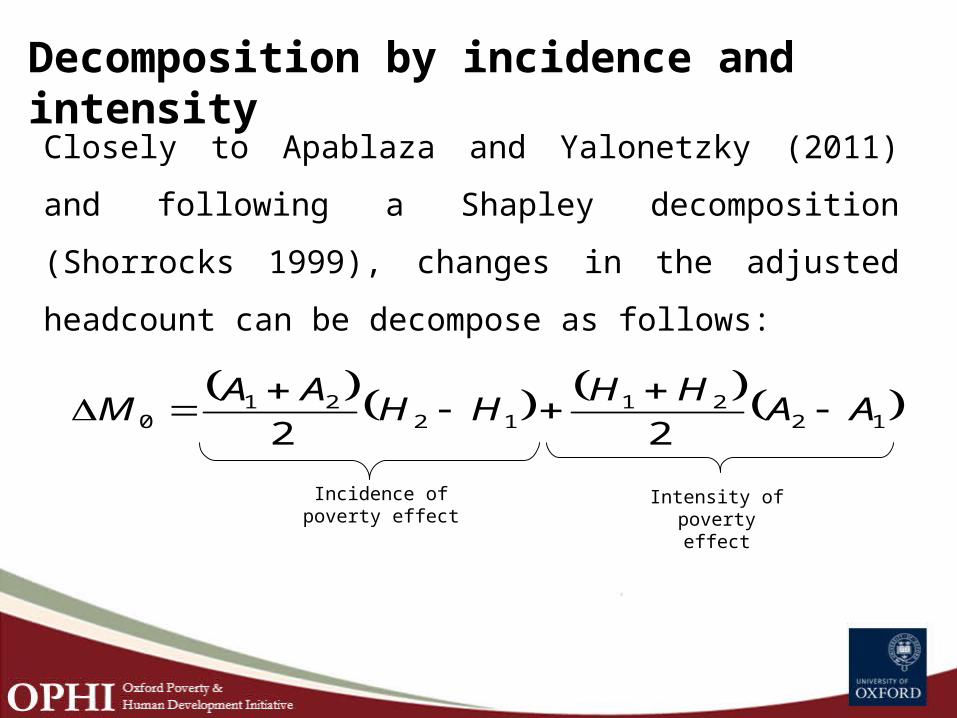
Decomposition by incidence and intensityClosely to Apablaza and Yalonetzky (2011) and
following a Shapley decomposition (Shorrocks
1999), changes in the adjusted headcount can be
decompose as follows:
Incidence ofpoverty effect
Intensity ofpoverty effect
1221
1221
0 22AA
HHHH
AAM
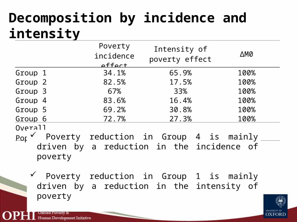
Decomposition by incidence and intensity
Poverty incidence effect
Intensity of poverty effect ΔM0
Group 1 34.1% 65.9% 100%Group 2 82.5% 17.5% 100%Group 3 67% 33% 100%Group 4 83.6% 16.4% 100%Group 5 69.2% 30.8% 100%Group 6 72.7% 27.3% 100%Overall Population 72.1% 27.9% 100%
Poverty reduction in Group 4 is mainly driven by a reduction in the incidence of poverty
Poverty reduction in Group 1 is mainly driven by a reduction in the intensity of poverty

Decomposition of the variation in intensity
of poverty by dimension

19
Variation in M0 and its components(figures from Roche 2013, Child Poverty)
Absolute Variation 1997 2000 1997-2000M0 0.555 0.495 -6%***H 82.9% 75.8% -7.1%***A 66.9% 65.3% -1.6%***
Raw Headcount ratio Health 43.5% 39.8% -3.7%**Nutrition 74.3% 62.2% -12.1%***Water 4.7% 3.6% -1.1%Sanitation 72.5% 68.4% -4.1%**Shelter 95.9% 94.1% -1.8%**Information 68.5% 65.3% -3.2%*
Censored Headcount ratio (Health 41.3% 37.1% -4.1%**Nutrition 68.4% 56.0% -12.5%***Water 4.6% 3.4% -1.2%Sanitation 69.8% 63.8% -6.0%***Shelter 82.6% 75.4% -7.3%***
Information 66.0% 61.3% -4.7%***
Note: *** statistically significant at α=0.01, ** statistically significant at α=0.05, * statistically significant at α=0.10
The raw and censored
headcount tells us about the
reduction in each dimension and its
relation to multidimensional
poverty reduction.
We can compute the
contribution of each dimension to changes in
intensity

Raw and Censored Headcount RatiosFrom previous sessions we know that…
Raw headcount: The raw headcount of dimension j represents the proportion of deprived people in dimension j, given by
Censored headcount: The censored headcount represents the proportion deprived and poor people in dimension j. It is computed from the censored deprivation matrix by
Intensity of poverty: The intensity of poverty is define as the average deprivations shared across the poor and is given by
ng
H jj
0
nkg
Ch jj
)(0
)()( qkcA
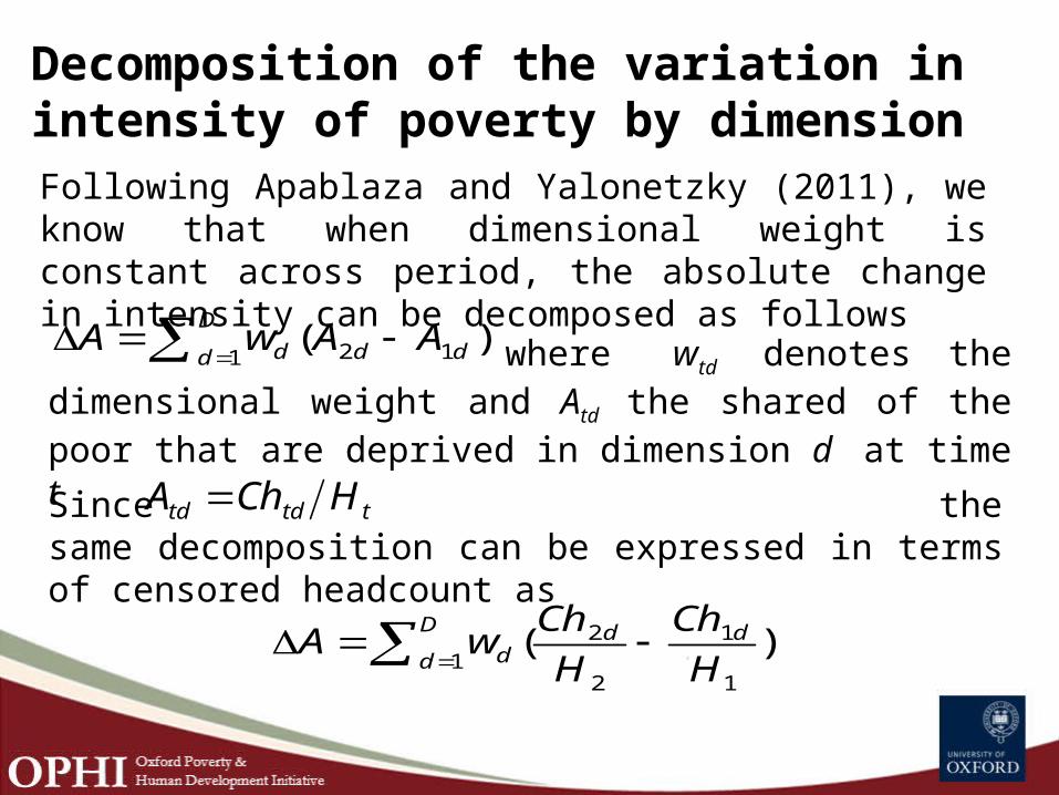
Decomposition of the variation in intensity of poverty by dimensionFollowing Apablaza and Yalonetzky (2011), we know that when dimensional weight is constant across period, the absolute change in intensity can be decomposed as follows
where wtd denotes the dimensional weight and Atd the shared of the poor that are deprived in dimension d at time t
)( 121 dd
D
d d AAwA
Since the same decomposition can be expressed in terms of censored headcount as
ttdtd HChA
)(1
1
2
2
1 H
Ch
H
ChwA ddD
d d

Decomposition by incidence and intensity(figures from Roche 2013, Child Poverty)
Absolute Variation 1997 2000 1997-2000M0 0.555 0.495 -6%***H 82.9% 75.8% -7.1%***A 66.9% 65.3% -1.6%***
Raw Headcount ratio Health 43.5% 39.8% -3.7%**Nutrition 74.3% 62.2% -12.1%***Water 4.7% 3.6% -1.1%Sanitation 72.5% 68.4% -4.1%**Shelter 95.9% 94.1% -1.8%**Information 68.5% 65.3% -3.2%*
Censored Headcount ratio Health 41.3% 37.1% -4.1%**Nutrition 68.4% 56.0% -12.5%***Water 4.6% 3.4% -1.2%Sanitation 69.8% 63.8% -6.0%***Shelter 82.6% 75.4% -7.3%***
Information 66.0% 61.3% -4.7%***
Note: *** statistically significant at α=0.01, ** statistically significant at α=0.05, * statistically significant at α=0.10
ContributionM0 100%H 72%A 28%ΔA 100%Health 63%Nutrition 24%Water 3%Sanitation 14%Shelter 0%Information -3%
The contribution helps to understand
the relation between changes in
multidimensional poverty and
changes in raw and censored
headcount. It helps to analyse this together as it is mediated by the
identification step
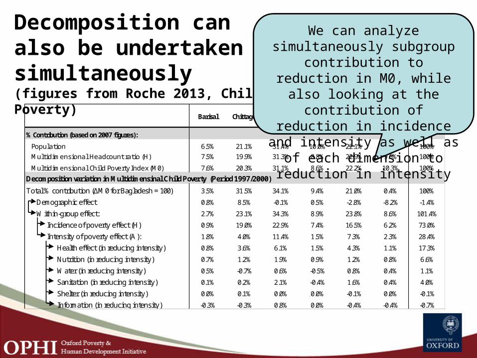
Decomposition can also be undertaken simultaneously(figures from Roche 2013, Child Poverty)
% Contribution (based on 2007 figures):
Population 6.5% 21.1% 31.4% 10.0% 22.1% 8.9% 100%Multidimens ional Headcount ratio (H) 7.5% 19.9% 31.3% 8.8% 22.9% 9.6% 100%
Multidimens ional Chi ld Poverty Index (M0) 7.6% 20.3% 31.1% 8.6% 22.2% 10.3% 100%
Decomposition variation in Multidimensinal Child Poverty (Period 1997/2000)
Total % contribution (ΔM0 for Bagladesh = 100) 3.5% 31.5% 34.1% 9.4% 21.0% 0.4% 100%
Demographic effect 0.8% 8.5% -0.1% 0.5% -2.8% -8.2% -1.4%
Within-group effect: 2.7% 23.1% 34.3% 8.9% 23.8% 8.6% 101.4%
Incidence of poverty effect (H) 0.9% 19.0% 22.9% 7.4% 16.5% 6.2% 73.0%
Intensity of poverty effect (A): 1.8% 4.0% 11.4% 1.5% 7.3% 2.3% 28.4%
Health effect (in reducing intensity) 0.8% 3.6% 6.1% 1.5% 4.3% 1.1% 17.3%
Nutrition (in reducing intensity) 0.7% 1.2% 1.9% 0.9% 1.2% 0.8% 6.6%
Water (in reducing intensity) 0.5% -0.7% 0.6% -0.5% 0.8% 0.4% 1.1%
Sanitation (in reducing intensity) 0.1% 0.2% 2.1% -0.4% 1.6% 0.4% 4.0%
Shelter (in reducing intensity) 0.0% 0.1% 0.0% 0.0% -0.1% 0.0% -0.1%
Information (in reducing intensity) -0.3% -0.3% 0.8% 0.0% -0.4% -0.4% -0.7%
BagladeshBarisal Chittago Dhaka Khulna Rajshahi Sylhet
We can analyze simultaneously subgroup
contribution to reduction in M0, while also looking at the contribution of reduction in incidence and intensity as
well as of each dimension to reduction in intensity

Suggestion1. The starting point is the simple analysis of variation of
changes in M0 and its elements – often it is informative to analyze both absolute and relative variation
2. Check for statistical significance of differences that are key for your analysis. Reporting the SE and/or Confidence Interval is a good practice so the reader can make other comparison
3. Undertake robustness test of the main findings (by range of weights, deprivation cut-off and poverty cut-offs)
4. The analysis of changes in M0 should be undertaken integrated with changes in its elements: incidence, intensity, and dimensional changes (it is useful to analyze both raw and censored headcount)
5. It is important for policy to differentiate the within group effect and demographic effect when analysing the contribution of each subgroup to overall change in Multidimensional Poverty. The demographic factors can further be studied with demographic data regarding population growth and migration.

Thank you
www.ophi.org.uk

APPENDIX:The AF method and two
points in time – variation in M0 and its constitutive
elements

The AF method and two points in time
xi1 xi2 xi3 xi4 xi5 Ci
g0: 0 0 0 0 0 00 1 0 0 0 10 1 1 0 0 21 1 1 0 1 41 1 1 1 1 5
RawH: 2/5 4/5 3/5 1/5 2/5
Time 1
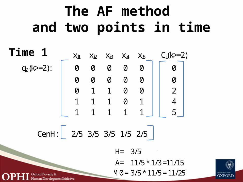
xi1 xi2 xi3 xi4 xi5 Ci(k>=2)
g0(k>=2): 0 0 0 0 0 00 0 0 0 0 00 1 1 0 0 21 1 1 0 1 41 1 1 1 1 5
CenH: 2/5 3/5 3/5 1/5 2/5
The AF method and two points in time
H= 3/5A= 11/5 * 1/3 =11/15
M0 = 3/5 * 11/5 = 11/25
Time 1
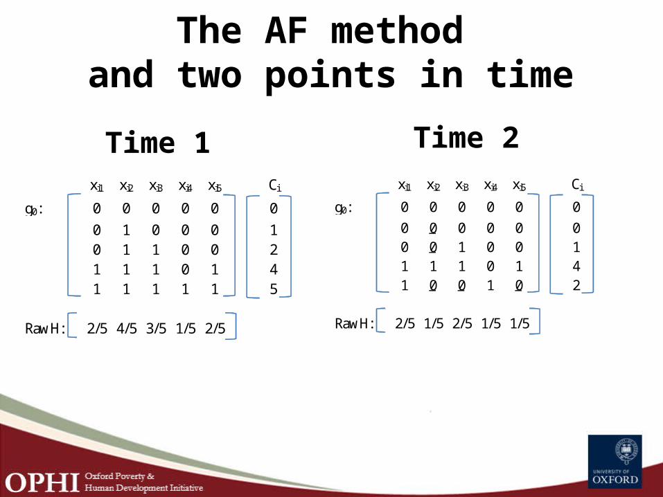
The AF method and two points in time
Time 2Time 1xi1 xi2 xi3 xi4 xi5 Ci
g0: 0 0 0 0 0 00 1 0 0 0 10 1 1 0 0 21 1 1 0 1 41 1 1 1 1 5
RawH: 2/5 4/5 3/5 1/5 2/5
xi1 xi2 xi3 xi4 xi5 Ci
g0: 0 0 0 0 0 00 0 0 0 0 00 0 1 0 0 11 1 1 0 1 41 0 0 1 0 2
RawH: 2/5 1/5 2/5 1/5 1/5

xi1 xi2 xi3 xi4 xi5 Ci(k>=2)
g0(k>=2): 0 0 0 0 0 00 0 0 0 0 00 0 0 0 0 01 1 1 0 1 41 0 0 1 0 2
CenH: 2/5 1/5 1/5 1/5 1/5
The AF method and two points in time
Time 2Time 1xi1 xi2 xi3 xi4 xi5 Ci(k>=2)
g0(k>=2): 0 0 0 0 0 00 0 0 0 0 00 1 1 0 0 21 1 1 0 1 41 1 1 1 1 5
CenH: 2/5 3/5 3/5 1/5 2/5
In this example we know how each individual have change over time, like in panel data, when using cross sectional data we do not have this level of detail.
H= 3/5A= 11/5 * 1/3 =11/15
M0 = 3/5 * 11/5 = 11/25
H= 2/5A= 6/5*1/2 = 6/10
M0 = 2/5 * 6/10 = 6/25

The AF method and two points in time: Consider ci vector or CH
vectorTime 2Time 1
H= 3/5A= 11/5 * 1/3 =11/15
M0 = 3/5 * 11/5 = 11/25
H= 2/5A= 6/5*1/2 = 6/10
M0 = 2/5 * 6/10 = 6/25
RawH: 2/5 4/5 3/5 1/5 2/5
0 0 1 0 0 11 1 1 0 1 41 0 0 1 0 2
RawH: 2/5 1/5 2/5 1/5 1/5
0 0 0 0 0 00 1 1 0 0 21 1 1 0 1 41 1 1 1 1 5
CenH: 2/5 3/5 3/5 1/5 2/5
0 0 0 0 0 00 0 0 0 0 01 1 1 0 1 41 0 0 1 0 2
CenH: 2/5 1/5 1/5 1/5 1/5
Variation
ΔRawH: 0 -3/5 -1/5 0 -1/5
ΔCenH: 0 -2/5 -1/5 0 -1/5
ΔH= -1/5ΔA= -2/15
ΔM0 = -5/15
It won’t stop here – we could also perform further analysis on inequality among the poor based on the ci vector or assessing changes
in association or joint distribution

Reporting changes in Censored Heacount
Time 2Time 1
0 0 0 0 0 00 1 1 0 0 21 1 1 0 1 41 1 1 1 1 5
CenH: 2/5 3/5 3/5 1/5 2/5
0 0 0 0 0 00 0 0 0 0 01 1 1 0 1 41 0 0 1 0 2
CenH: 2/5 1/5 1/5 1/5 1/5
Variation
ΔCenH: 0 -2/5 -1/5 0 -1/5
Computing change
ΔX=(X2-X1)
-6
-5
-4
-3
-2
-1
0
Ghana Nigeria Ethiopia
Ann
ualiz
ed A
bsol
ute
Cha
nge
in th
e Pe
rcen
tage
Who
is P
oor a
nd D
epriv
ed in
...
Assets
Cooking Fuel
Flooring
Safe Drinking WaterImproved SanitationElectricity
Nutrition
Child Mortality
School AttendanceYears of Schooling


