Sunlight refraction in the mesosphere of Venus during the transit on June 8th, 2004

P. Tanga a,!, T. Widemann b, B. Sicardy b, J.M. Pasachoff c, J. Arnaud d,1, L. Comolli e, A. Rondi f, S. Rondi f,P. Sütterlin g,2

a Laboratoire Cassiopée UMR6202, Université de Nice Sophia-Antipolis, CNRS, Observatoire de la Côte d’Azur, BP 4229, 06304 Nice Cedex 4, Franceb LESIA-Observatoire de Paris, CNRS, UPMC Université Paris 6, Université Paris-Diderot, 5, place Jules Janssen, 92195 Meudon Cedex, FrancecWilliams College Hopkins Observatory, Williamstown, MA 01267-2565, USAd Laboratoire Fizeau UMR6525, Université de Nice Sophia-Antipolis, CNRS, Observatoire de la Côte d’Azur, BP 4229, 06304 Nice Cedex 4, FranceeGruppo Astronomico Tradatese, Via Mameli 13, 21049 Tradate, Italyf Société Astronomique de France, 3 rue Beethoven, 75016 Paris, Franceg Sterrekundig Institut, Utrecht University, Postbus 80 000, 3508 TA Utrecht, The Netherlands

a r t i c l e i n f o

Article history:Received 29 July 2011Revised 1 December 2011Accepted 1 December 2011Available online 20 December 2011

Keywords:VenusVenus, AtmosphereAtmospheres, Structure

a b s t r a c t

Many observers in the past gave detailed descriptions of the telescopic aspect of Venus during its extre-mely rare transits across the Solar disk. In particular, at the ingress and egress, the portion of the planet’sdisk outside the Solar photosphere has been repeatedly perceived as outlined by a thin, bright arc (‘‘aure-ole’’). Those historical visual observations allowed inferring the existence of Venus’ atmosphere, thebright arc being correctly ascribed to the refraction of light by the outer layers of a dense atmosphere.On June 8th, 2004, fast photometry based on electronic imaging devices allowed the first quantitativeanalysis of the phenomenon. Several observers used a variety of acquisition systems to image the event– ranging from amateur-sized to professional telescopes and cameras – thus collecting for the first time alarge amount of quantitative information on this atmospheric phenomenon. In this paper, after reviewingsome elements brought by the historical records, we give a detailed report of the ground based observa-tions of the 2004 transit. Besides confirming the historical descriptions, we perform the first photometricanalysis of the aureole using various acquisition systems. The spatially resolved data provide measure-ments of the aureole flux as a function of the planetocentric latitude along the limb. A new differentialrefraction model of solar disk through the upper atmosphere allows us to relate the variable photometryto the latitudinal dependency of scale-height with temperature in the South polar region, as well as thelatitudinal variation of the cloud-top layer altitude. We compare our measurements to recent analysis ofthe Venus Express VIRTIS-M, VMC and SPICAV/SOIR thermal field and aerosol distribution. Our resultscan be used a starting point for new, more optimized experiments during the 2012 transit event.

! 2011 Elsevier Inc. All rights reserved.

1. Introduction

Since the mid 18th century, observers have reported unusualfeatures of the telescopic image of Venus near the inferior conjunc-tion, promptly attributed to its atmosphere. Some of them are atthe reach of modest instruments (although at small angular dis-tance from the Sun), such as the cusp extension first describedby Schroeter (1791), which tends to transform the thin crescentof Venus into a ring of light (e.g. Russell, 1899; Dollfus andMaurice, 1965).

One of the most relevant features pertaining to ground-basedstudies of the Venus atmospheric structure has been observed only

during transits, close to the phases of ingress (between 1st and 2ndcontact) and egress (between 3rd and 4th contact) as a bright arcoutlining – in part or entirely – the portion of Venus’ disk projectedoutside the solar photosphere. Traditionally the first account of thisphenomenon was attributed to Mikhail V. Lomonosov (1711–1765)who reported his observations of the transit at St. Petersburg Obser-vatory on May 26, 1761 (Marov, 2005). Actually the poor perfor-mance of his small refractor hints that most probably otherobservers (such as Chappe d’Auteroche, Bergman, and Wargentin)were the first genuine witness on the same date (Link, 1969; Pasac-hoff and Sheehan, 2012). However, Lomonosov correctly attributedthe putative phenomenon to the presence of an atmosphere aroundthe planet, refracting the sunlight in the observer’s direction.

In the following, adopting a denomination widely used in thehistorical accounts, we will often call this arc ‘‘aureole’’. Since boththe aureole and the cusp extension occur close to the planet termi-nator, they are also collectively known as ‘‘twilight phenomena’’.For detailed historical reviews the interested reader can refer to

0019-1035/$ - see front matter ! 2011 Elsevier Inc. All rights reserved.doi:10.1016/j.icarus.2011.12.004

! Corresponding author.E-mail address: Paolo.Tanga@oca.eu (P. Tanga).

1 Deceased on September 11, 2010.2 Present address: Institute for Solar Physics, The Royal Swedish Academy of

Sciences, Alba Nova University Center, 106 91 Stockholm, Sweden.

Icarus 218 (2012) 207–219

Contents lists available at SciVerse ScienceDirect

Icarus

journal homepage: www.elsevier .com/locate / icarus

Link (1969) and Edson (1963). Of course, in this context we neglectthe initial motivation for the observation of transits: the determi-nation of the Astronomical Unit by the solar parallax (proposedby E. Halley in 1716), whose interest is purely historical today.

Venus transits are rare, as they occur in pairs 8 years apart, eachpair separated by 121.5 or 105.5 years, alternating betweendescending node (June pairs: 1761/1769, 2004/2012,. . .), andascending node (December pairs: 1631/1639, 1874/1882, 2117/2125,. . .). As a consequence, data concerning the aureole are corre-spondingly sparse and, up to the last event, they have been obtainedby simple visual inspection,mainly by using refracting telescopes ofmodest aperture (typically up to 15–20 cm). This limitation wasmainly due to the constraint of organizing complex expeditionsincluding the delicate transportation of all the instruments.

The 2004 event represents a giant leap in the observation ofVenus transits, as the modern imaging technologies available allowfor the first time a quantitative analysis of the atmospheric phe-nomena associated to the transit of Venus.

We performed measurements of the aureole on the originalimages obtained through several different instruments, and com-pared them both with a simple refraction model and with observa-tions obtained in the past. This work summarizes the aspect ofVenus close to the Sun’s limb during the June 8, 2004 transit as ob-served by ground-based instruments. A recent paper (Pasachoffet al., 2011) deals with imaging using NASA’s then operating Tran-sition Region and Coronal Explorer solar observatory (TRACE).

Since the ground-based observations were not specifically orga-nized beforehand, data at our disposal are rather heterogenous. Inorder to bridge the gap between past visual observations throughsmall telescopes and today’s technologies, we decided to consideraccounts obtained both with professional instruments and low-cost amateur telescopes, either by CCD imaging or by direct imageinspection by experienced observers. In fact, as shown in recentstudies of distant Solar System objects based on stellar occultationcampaigns (e.g. Widemann et al., 2009) while CCD imaging offerstoday the most valuable quantitative measurements, small tele-scopes and visual observations allow a significant increase of con-strains on the phenomena – and in the case of Venus, the mostdirect comparison to past reports. The results obtained from theanalysis of the most significant image sets, representing a certainvariety of instrument size and quality, are illustrated in this paper.

The paper is organized as follows. First, we describe the condi-tions of the 2004 event, and the reconstruction of limb geometry(Section 2). We then provide an extensive review of the measuredspatial and temporal variations for the brightness of the aureoleinwide or narrow-band photometry (Sections 3 and 4).We then ad-dress the basic physical principles of the atmospheric differentialrefraction model producing the aureole (Section 5) and we use itfor the interpretation of the observations (6). In Section 7, the mod-eling of the aureole is compared to recent analysis of the Venus Ex-press observations (VIRTIS-M, VeRa and SPICAV/SOIR) regardingthe thermal field and cloud-deck altitude and haze distribution per-taining to this study, as well as ground-based mid-infrared spec-troscopy of non-LTE CO2 emission. The comparison is discussed.

2. Geometry of the transit in 2004

For simplicity and following Link (1969) hereinafter we call‘‘phase’’ (f) of the event the fraction of Venus diameter externalto the solar photosphere. A value f = 0 corresponds to the planetentirely projected on the Sun, tangent to its limb. When f = 0.5,the planet centre will be exactly on the solar limb, and so on.

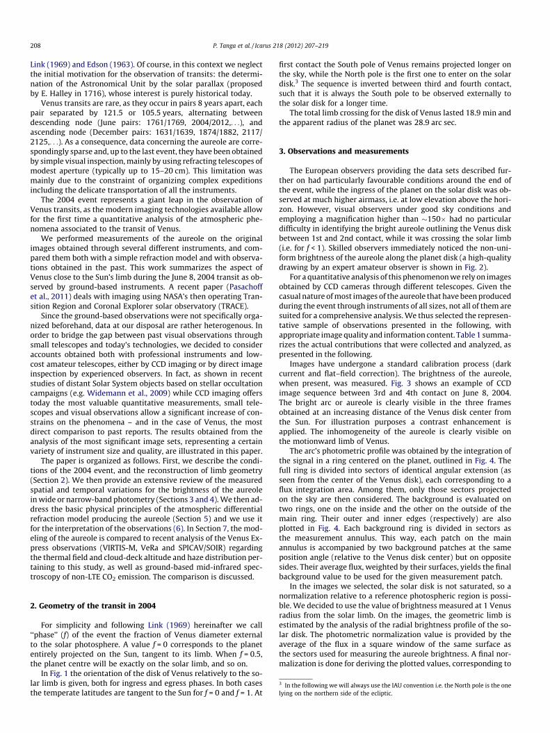
In Fig. 1 the orientation of the disk of Venus relatively to the so-lar limb is given, both for ingress and egress phases. In both casesthe temperate latitudes are tangent to the Sun for f = 0 and f = 1. At

first contact the South pole of Venus remains projected longer onthe sky, while the North pole is the first one to enter on the solardisk.3 The sequence is inverted between third and fourth contact,such that it is always the South pole to be observed externally tothe solar disk for a longer time.

The total limb crossing for the disk of Venus lasted 18.9 min andthe apparent radius of the planet was 28.9 arc sec.

3. Observations and measurements

The European observers providing the data sets described fur-ther on had particularly favourable conditions around the end ofthe event, while the ingress of the planet on the solar disk was ob-served at much higher airmass, i.e. at low elevation above the hori-zon. However, visual observers under good sky conditions andemploying a magnification higher than !150" had no particulardifficulty in identifying the bright aureole outlining the Venus diskbetween 1st and 2nd contact, while it was crossing the solar limb(i.e. for f < 1). Skilled observers immediately noticed the non-uni-form brightness of the aureole along the planet disk (a high-qualitydrawing by an expert amateur observer is shown in Fig. 2).

For a quantitative analysis of this phenomenonwe rely on imagesobtained by CCD cameras through different telescopes. Given thecasual nature ofmost images of the aureole that have beenproducedduring the event through instruments of all sizes, not all of them aresuited for a comprehensive analysis.We thus selected the represen-tative sample of observations presented in the following, withappropriate image quality and information content. Table 1 summa-rizes the actual contributions that were collected and analyzed, aspresented in the following.

Images have undergone a standard calibration process (darkcurrent and flat–field correction). The brightness of the aureole,when present, was measured. Fig. 3 shows an example of CCDimage sequence between 3rd and 4th contact on June 8, 2004.The bright arc or aureole is clearly visible in the three framesobtained at an increasing distance of the Venus disk center fromthe Sun. For illustration purposes a contrast enhancement isapplied. The inhomogeneity of the aureole is clearly visible onthe motionward limb of Venus.

The arc’s photometric profile was obtained by the integration ofthe signal in a ring centered on the planet, outlined in Fig. 4. Thefull ring is divided into sectors of identical angular extension (asseen from the center of the Venus disk), each corresponding to aflux integration area. Among them, only those sectors projectedon the sky are then considered. The background is evaluated ontwo rings, one on the inside and the other on the outside of themain ring. Their outer and inner edges (respectively) are alsoplotted in Fig. 4. Each background ring is divided in sectors asthe measurement annulus. This way, each patch on the mainannulus is accompanied by two background patches at the sameposition angle (relative to the Venus disk center) but on oppositesides. Their average flux, weighted by their surfaces, yields the finalbackground value to be used for the given measurement patch.

In the images we selected, the solar disk is not saturated, so anormalization relative to a reference photospheric region is possi-ble. We decided to use the value of brightness measured at 1 Venusradius from the solar limb. On the images, the geometric limb isestimated by the analysis of the radial brightness profile of the so-lar disk. The photometric normalization value is provided by theaverage of the flux in a square window of the same surface asthe sectors used for measuring the aureole brightness. A final nor-malization is done for deriving the plotted values, corresponding to

3 In the following we will always use the IAU convention i.e. the North pole is the onelying on the northern side of the ecliptic.

208 P. Tanga et al. / Icarus 218 (2012) 207–219

256°.46

6°.13

Fig. 1. Sketch of Venus’ disk orientation at the ingress (left panel) or egress (right) of the transit. The grayed area corresponds to the Sun’s photosphere at the epoch when theVenus disk is externally tangent to the Sun (first and fourth contact: t1 and t4 respectively). The solar limb is also indicated at the second and third contact (labeled t2 and t3)and when projected on the center of Venus. The solid arrows indicate the direction of the apparent motion of the planet relative to the Sun. The vertical dashed linecorresponds to the sky North–South direction, while the dash-dotted one represents the sky-projected rotation axis of Venus.

Fig. 2. Drawings of Venus at the beginning (three leftmost panels) and end of the event (remaining two panels), as seen visually by an expert amateur astromer (MarioFrassati, Italy) through a 20 cm Schmidt-Cassegrain telescope. Courtesy of the archive of Sezione Pianeti, Unione Astrofili Italiani.

Table 1Measured observations. The availability of ingress (‘‘In’’ column) or egress (‘‘Ex’’) images is given. The number of measured images follows. These are final images, as a result of anaveraging process when needed. The final column identifies the filter name and/or their central wavelength/width. See case by case detailed explanations in the text.

Observer Instrument Site In Ex No. images k/FWHM (nm)

J. Arnaud Themis Tenerife (Spain) – X 50 VL. Comolli 20 cm Schmidt-Cass. Tradate (Italy) X X 50 VP. Suetterlin DOT La Palma (Spain) X 21 430.5/1.0, G

X 21 431.9/0.6, Blue cont.X 21 655.0/0.6, Red cont.X 21 396.8/0.1, Ca II H

S. Rondi 50 cm Tourelle refr. Pic du Midi (France) X 32 NaD1/10

Fig. 3. Three images concerning the final phases of the transit obtained by the DOT telescope in the ‘‘G’’ band. Each image has been altered in contrast (gamma = 0.4) in orderto better show the thin and faint arc of light outlining (partially or completely) the Venus limb. The orientation is the same as in Fig. 1. The bright saturated area is the solarphotosphere. The progressive reduction in extension and brightness of the aureole with time is clearly visible.

P. Tanga et al. / Icarus 218 (2012) 207–219 209

the flux coming from an unresolved, thin segment of aureole 1 arc-sec in length, normalized to the brightness of a square patch ofphotosphere having a surface of 1 arcsec2.

In the following, we present technical details of each data set,with the corresponding aureole luminosity derived. The error barsgiven in the plots are computed by considering the Poissonian sta-tistics of the photometric noise. We indicate by Ns and Nb the num-ber of photoelectrons coming from the aureole and the background,respectively, in each arc bin. The uncertainty that we consider isr = (Ns + Nb)0.5. In our case, Nb # Ns, thus the only relevant contri-bution to noise comes from the background, and is a function ofthe distance of the arc element from the solar limb. The cameraread-out-noise is cleary smaller than the background contributionand can be discarded as well. The same applies to noise associatedto the dark current, since exposure times are extremely short.

From a practical point of view, we have verified that r appearsto be fairly constant over the entire arc, growing of about 50% onlyfor measurement points very close to the solar limb. For this rea-son, we choose to show only one error bar, common to all curves,except in the case of observations obtained at the DOT telescopewhich are used for modelling the aureole flux. In the related plots,two error bars separately for low and high f values, provide anadditional information on the amount of noise variation in time.

3.1. Tourelle Solar Telescope – Pic du Midi, France

Only the ingress has been imaged by this station, since cloudshave prevented a clear view of the final phases. Given the imagescale, the radius of Venus is 142.5 pixels. For a set of selectedimages in which the aureole is well visible at the visual inspection,its integrated flux was determined using different widths of themeasuring ring, from 2 to 14 pixel. The resulting ‘‘growth curve’’

(Howell, 1989) shows the convergence toward the inclusion ofthe complete flux coming from the arc. The flux was consideredto be completely inside the ring at a width of 9 pixel, then usedfor all measurements. The arc was sampled at angular steps of 9".

Also, it was found that due to the faintness of the aureole, a use-ful improvement of the SNR was obtained by averaging images bygroups of 3. The final image set obtained this way was much easierto measure than the original single frames. In the following discus-sion of Pic du Midi data we call ‘‘images’’ the members of this finalset.

The arc is present on 16 images, and a photometric profile wasderived for each. Given the poor signal-to-noise ratio (SNR) thecurves were later average by four, obtaining the result presentedin Fig. 5. The profiles have been trimmed in order to exclude theregion in which the measurement areas (main or backgroundpatch) are contaminated by the photosphere. In other words, onlythe portion corresponding to the arc projected on the sky is plot-ted. In the case of the Tourelle telescope, the background stronglycontaminates the signal when the planet is about halfway into theingress. We thus had to be very conservative concerning the frac-tion of arc to be considered.

Despite the averaging, the result is still affected by a significantnoise, as indicated by the size of the vertical bars in Fig. 5, repre-senting the 1-sigma level. For this reason, small scale fluctuationsin the brightness profile probably do not have a strong statistic sig-nificance if considered separately. However, some general trendsare present and repeat from one curve to the other. For example,a general slope of the curve bottom is present. Also, at large valuesof f (lowest curves) a maximum in intensity is detectable close tothe South pole of the planet. Interestingly, the maximum is not ex-actly centered on the pole, a feature that repeats in the other datasets described further on. The intensity minimum coincides ratherwell with the position angle of the equator of Venus (bar on theleft). Even at later times, represented by the curves at the highestvalues, the trend of growing brightness toward the pole is present.In all cases, if we neglect the extreme tips of the arc very close tothe photosphere, the aureole flux is less than about 2% the photo-spheric value, and is detectable down to about 0.2%.

N

Fig. 4. Scheme of the procedure adopted for the measurements and implementedin a custom software. Here black is used to represent the sky background and thedisk of Venus. The four white circles define three concentric rings, with the aureoleentirely contained in the central one. The nearby external and internal rings areused for evaluating the background. Each ring is divided in sectors of equal angularsize. One of them is represented for the aureole (solid rectangle) and thecorresponding background areas (dotted). The dashed angle represents the positionangle (relative to the celestial North) used for representing the brightness profiles infollowing plots. The dashed-dotted line represents the orientation of the rotationaxis of Venus.

Fig. 5. Photometric profile of the aureole during ingress, obtained at the Tourelletelescope, Pic du Midi. The plotted value represents the flux coming from a segmentof 1 arcsec of the aureole, normalized to the flux coming from a 1 arc sec2 surface ofthe solar photosphere at 1 Venus radii from the solar limb (measured on the sameset of images). The horizontal axis shows the position angle along the Venus limb,with the usual conventions in the equatorial reference: origin of angles at thecelestial N, increasing toward E. The two vertical lines represent the position angleof the equator (left, ‘‘E’’ label) and the South pole (right, ‘‘S’’). The flux from theaureole increases with time. Upper curves, with the planet about halfway across thesolar limb, cover a short angular range since their extremes are strongly contam-inated by a high background. Labels indicate the values of f associated to each curve.

210 P. Tanga et al. / Icarus 218 (2012) 207–219

3.2. 20 cm Schmidt-Cassegrain-Tradate, Italy

L. Comolli observed the event by a digital video-camera, withexposure times variable between 1/2000 and 1/50 s. Only the short-est exposures have been used, since they do not present saturationon the solar photosphere, thus allowing a normalization equivalentto those presented in the other cases. Each analyzed image is the re-sult of the sumof the best 200–300 frames over!1 minof recording.

Both ingress and egress were imaged and analyzed, using a stepof 4.5" over the Venus limb. The measured flux distribution duringegress is well consistent with DOT data (presented below), but lim-ited by a far lower resolution. For this reason they are not plottedhere. More interesting is the comparison of the ingress luminosityprofiles to the results obtained by the Tourelle Solar Telescopeimages.

Five profiles were obtained and are presented in Fig. 6. Theyconfirm, from both the point of view of the distribution and theflux values, the data obtained at the Tourelle telescope. Discrepan-cies around 15% at f ! 0.5 in the faintest part of the aureole appearsmall when taking into account the wide difference in equipmentand site, however they clearly hint to the difficulty of obtainingclean and appropriate signals at such small solar elongations.

3.3. Themis Solar Telescope – Pico del Teide Observatory, Tenerife,Spain

Themis data are complementary to the Pic duMidi observations,since fromthis site itwas the exit phase to be imaged, both throughanarrow-bandH-alfa filter and a filter centered at 430 nm. The imagesampling is lower (Venus radius!70 pixels) but a large image rate isavailable (1 image each 1.06 s). The sequence was thus divided intodifferent sets of images, containing 20–60 frames each. The mostpopulatedsets correspond to the largest valuesof f, containinganex-tremely faint aureole slowly fading into the background.

Inside each set, each image was re-sampled with a re-alignmentof the disk of Venus relatively to an image chosen as reference. Anautomated procedure based on the computation of cross-correla-tions by Fast Fourier Transforms was used, providing the shift toapply to each image. Small relative image drifts are thus mini-mized and the SNR of the faint arc is preserved during the sum-ming procedure that yields a final image for each set.

In this way, 50 images were derived from the sum of the framesinside each set, and measured as those of the previous section. Thenormalization procedure adopted was also the same. Due to poorseeing, a width of 7 pixels was needed to include the entire flux.

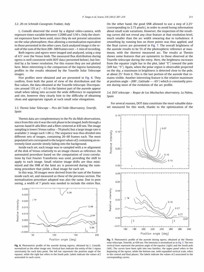
On the other hand, the good SNR allowed to use a step of 2.25"(corresponding to 2.75 pixels), in order to avoid losing informationabout small scale variations. However, the inspection of the result-ing curves did not reveal any clear feature at that resolution level,much smaller than the arc width smearing due to turbulence. Asmoothing by running box on three points was thus applied, andthe final curves are presented in Fig. 7. The overall brightness ofthe aureole results to be 5% of the photospheric reference at max-imum, with the shortest measured arc. The results at Themisshows some features that are symmetric to those observed at theTourelle telescope during the entry. Here, the brightness increasesfrom the equator (right bar in the plot, label ‘‘E’’) toward the pole(left bar, ‘‘S’’). Again, when the polar region is observable projectedon the sky, a maximum in brightness is detected close to the pole,at about 25" from it. This is the last portion of the aureole that re-mains visible. Another interesting feature is the relative maximumat position angle !200", (latitude !$65") which is constantly pres-ent during most of the evolution of the arc profile.

3.4. DOT telescope – Roque de Los Muchachos observatory, La Palma,Spain

For several reasons, DOT data constitute the most valuable data-set measured for this work, thanks to the optimization of the

Fig. 6. Photometric profile of the aureole during ingress, obtained by L. Comolli,normalized as the other image sets. Vertical bars indicate the entity of the 1-sigmauncertainty for each data point. The left bar represents the position angle of theequator, while the right bar refers to the South pole. Labels indicate the values of fassociated to each curve.

Fig. 7. Photometric profile of the aureole during egress, obtained at the Themissolar telescope, Tenerife, at 430 nm. The intensity is normalized as in Fig. 5. The twovertical lines represent the position angle of the equator (right) and the South pole(left). The curves have been split into two families: the upper panel refers to thebeginning of the egress, while the bottom one, with expanded vertical scale, refersto the central and final phases. The labels indicate the values of f associated to thecorresponding curves.

P. Tanga et al. / Icarus 218 (2012) 207–219 211

instrument for solar observations (Bettonvil et al., 2003; Ruttenet al., 2004). First of all, the image sampling (0.07 arcsec/pixel) pro-vides a comfortable scale for measurements, resulting in a Venusdisk with a radius of 415 pixels. Also, images in four narrow bands(usually employed for solar studies) are available, all having aFWHM of 1 nm or less (Table 1). Four cameras were workingsimultaneously in the four bands, taking every minute an imageburst of 100 frames at 6 frames/s. For our measurements, allframes of each burst have been aligned and summed up to obtaina single image each minute. Due to very strong turbulence thealignment process has been very critical, and was obtained byapplying a Sobel edge enhancement filter with a threshold andthen using the Hough transform (Yuen et al., 1989) to find the pre-cise position of the disk of Venus in each image.

Fluxes were obtained for both the aureole and the backgroundwith the same method as with the previous data set. A step of 2"along the Venus limb was used for measurements. We show inFig. 8 the photometric profile referred to the G band. This resultis very similar to both the blue and red continuum images (Figs.9 and 10). Only in the Ca II H band (Fig. 11) some differences ap-pear under the form of additional peaks in the profile. Although asignature of high-contrast chromospheric structures in their re-fracted image cannot be completely ruled out, those features aremost probably related to the inner corona extending outward fromthe solar limb and contaminating the signal of the aureole, since itsflux cannot be easily excluded from the measurement areas.

However, as far as the main features are concerned, they arevery similar in all the four bands. For example, in all of them theshape of the profile soon after the third contact (first curves in

Fig. 8. Photometric profile of the aureole during egress, obtained at the DOT solartelescope, La Palma, in the G band. The intensity is normalized as in Fig. 5. The twovertical lines represent the position angle of the equator (right) and the South pole(left). The curves have been split into two families: the upper panel refers to thebeginning of the egress, while the bottom one, with expanded vertical scale, refersto the central and final phases. The time interval between each curve is 60 s. For aneasier visibility of the bottom panel, each curve has a step of 7 " 10$4 added inintensity relatively to its lower neighbor. The labels indicate the values of fassociated to the corresponding curves. Two levels of uncertainty (r) related to aposition angle in the range 150–250" are given in the two panels. The upper one isapplicable to values of f < 0.4, while the other one refers to f = 0.7.

Fig. 9. As in Fig. 8 in the blue continuum at 431.9 nm.

Fig. 10. As in Fig. 8 in the red continuum at 655 nm. Relative to the otherwavelength bands, here three curves are missing due to corrupted data files.

212 P. Tanga et al. / Icarus 218 (2012) 207–219

the upper panel, Fig. 8) has a similar shape, showing a bump athigh negative latitudes. This aspect is consistent with the observa-tions obtained at the Themis telescope. This maximum of luminos-ity at later phases is located between 160 and 210 degrees ofposition angle, and appears to have a double peak.

Compared to the Themis data, the DOT curves show an overalllower signal. Their internal consistency and the difficulties encoun-tered in measuring the Themis images affected by poor seeing sug-gest that the DOT measurements are probably much more reliable.Also, the low-resolution images by Comolli confirm the flux valuesobtained for the DOT. For these reasons, this data set is chosen forthe detailed analysis in the following.

4. Lightcurves and colors

In order to study a possible wavelength dependence of the aure-ole and its variation in time, we used the DOT images for the egressphase. Thefluxwasmeasuredon three arc segments centered on thepole, on the brightest part of the aureole at position angle 195" (posi-tion A) and on the faintest part at 218" (position B) as shown in thescheme of Fig. 12. Point B corresponds to a region at latitude 45"S.

The measurements were made on arc lengths of 10 degrees, inthe G band, blue and red continuum. The results are shown inFig. 13. On all the three plots, different wavelengths appear to fol-low a similar trend. This is expected especially for the blue contin-uum and the G band, which are very close in wavelength.

The fastest fall of flux in red continuum beyond t ! 12 min is afeature common to all the light curves, suggesting a certainchromaticity of the aureole. However, the related error bars arevery large in this interval. At the same time, images aroundt ! 9–10 min are affected by a momentary seeing worsening, soeven the color differences at these epochs are to be consideredwith caution. Also, the divergence of the blue and G fluxes beyondt ! 11 min is almost certainly spurious (due to the similarwavelength) and further underlines the difficulty of comparingvery low fluxes.

In conclusion, we cannot firmly state that the images at our dis-posal reveal a significant departure of the aureole color from thesolar spectrum.

5. Modeling the aureole

5.1. The refraction model

The aureole observed during Venus transits can be explained bythe refraction of solar rays through the planet outer atmosphericlayers. The rays that pass closer to the planet center are more devi-ated by refraction than those passing further out. The image of agiven solar surface element is flattened perpendicularly to Venus’limb by this differential deviation, while conserving the intensityof the rays, i.e. the brightness of the surface element per unit sur-face. This holds as long as the atmosphere is transparent, i.e. aboveabsorbing clouds or aerosol layers.

The refractive deviation of light is related to the physical struc-ture of the planet atmosphere. The formalism of this deviation hasbeen studied by Baum and Code (1953), for the cases of stellar occ-ultations by planets. Their approach assumes that (i) the local den-sity scale height H of the atmosphere is constant and much smallerthan the planet radius Rv, (ii) the atmosphere is transparent, (iii)and it has spherical symmetry.

This approach is still valid in our case, but has to be modified toaccount for the finite distance and size of the Sun. In the followingwe will consider that the physical properties of the transparentatmospheric layers vary smoothly with altitude, and remain aboutconstant over a scale height. Note that the assumption H% Rv isvalid here, as H is smaller than the atmospheric layer of Venus,in turn % the planet radius. Note also that the locally sphericalsymmetry is achieved for Venus’ atmosphere. As to the transpar-ency assumption, it must be dropped when the rays are going deepenough for the atmosphere to become opaque.

We model the aureole brightness as follows:

(1) We consider a surface element dS on the Sun. A ray emittedby dS will reach the observer O after being refracted by anangle x in Venus’s atmosphere (see Fig. 14). Note that we

Fig. 11. As in Fig. 8 in the Ca II band at 396.8 nm.

Fig. 12. Geometry at f = 0.5 during the final phases of the event. The large dotsindicate the points that where chosen for studying the variation of the arcbrightness in time. A corresponds to the brightest portion, and B to the faintest.

P. Tanga et al. / Icarus 218 (2012) 207–219 213

adopt here the convention x 6 0. To each element dS corre-sponds an image dS0 that will appear as an aureole nearVenus’s limb (Fig. 15).During its travel to Earth, the ray passes at a closest distanceof r from the planet center. Furthermore, dS projects itself ata distance ri from Venus’ center C, as seen from O. Note thatri is an algebraic quantity which is negative if dS and dS0 pro-ject themselves on opposite side relative to the planet centerC, and positive otherwise, see Figs. 14 and 15.

(2) The refraction angle x is given by Baum and Code (1953):

x & $m'r(!!!!!!!!!!!!!!!2pr=H

p; '1(

where m is the gas refractivity, decreasing exponentially withr. This quantity is related to the gas number density n bym = K ) n, where K is the specific refractivity. For CO2, we have4

K = 1.67 " 10$29 m3 molecule$1.(3) It can be shown that surface element dS0 is radially shrunk

with respect to dS by a factor U = 1/[1 + D ) (@x/@r)], whereD is the distance from Venus to Earth. Note that since theatmosphere is assumed to have a constant density scaleheight, @x/@r = $x/H, thus:

D' D

r

ri

Sun

surfa

ce

Venus

observerC

dS

dS'

O

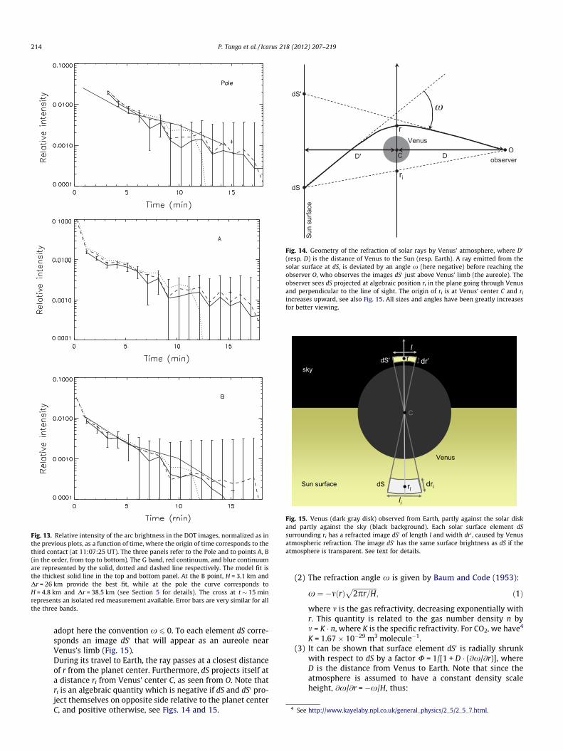
Fig. 14. Geometry of the refraction of solar rays by Venus’ atmosphere, where D0

(resp. D) is the distance of Venus to the Sun (resp. Earth). A ray emitted from thesolar surface at dS, is deviated by an angle x (here negative) before reaching theobserver O, who observes the images dS0 just above Venus’ limb (the aureole). Theobserver sees dS projected at algebraic position ri in the plane going through Venusand perpendicular to the line of sight. The origin of ri is at Venus’ center C and riincreases upward, see also Fig. 15. All sizes and angles have been greatly increasesfor better viewing.

Fig. 13. Relative intensity of the arc brightness in the DOT images, normalized as inthe previous plots, as a function of time, where the origin of time corresponds to thethird contact (at 11:07:25 UT). The three panels refer to the Pole and to points A, B(in the order, from top to bottom). The G band, red continuum, and blue continuumare represented by the solid, dotted and dashed line respectively. The model fit isthe thickest solid line in the top and bottom panel. At the B point, H = 3.1 km andDr = 26 km provide the best fit, while at the pole the curve corresponds toH = 4.8 km and Dr = 38.5 km (see Section 5 for details). The cross at t ! 15 minrepresents an isolated red measurement available. Error bars are very similar for allthe three bands.

r

ri

C

Sun surface

Venus

sky

dri

dr’

dS

dS'

l

li

Fig. 15. Venus (dark gray disk) observed from Earth, partly against the solar diskand partly against the sky (black background). Each solar surface element dSsurrounding ri has a refracted image dS0 of length l and width dr0 , caused by Venusatmospheric refraction. The image dS0 has the same surface brightness as dS if theatmosphere is transparent. See text for details.

4 See http://www.kayelaby.npl.co.uk/general_physics/2_5/2_5_7.html.

214 P. Tanga et al. / Icarus 218 (2012) 207–219

U & 11$ Dx=H

'2(

(4) It is convenient to take as a reference radius the closestapproach distance r1/2 corresponding toU = 0.5 (so so-called‘‘half-light radius’’ in the stellar occultation context). Thusx1/2 = $H/D. Re-arranging the various equations given

above, one finds K ) n1=2 &!!!!!!!!!!!!!!!!!!!!!!!!!!!!!!!H3='2pr1=2D2(

q, where n1/2 is

the gas number density at r1/2. The latter equation permitsto derive the numerical value of the half-light radius, oncean atmospheric model of the planet is given, that is, oncethe density profile n(r) is specified.

(5) From Eq. (1), we derive:

x & $HD) e$'r$r1=2(=H '3(

Simple geometrical consideration show that we also have:x = $k(r $ ri)/D, where k = 1 + D/D0 (D0 being the distance of Venusto the Sun). Combining this equationwithEqs. (2) and (3),weobtain:

1k

1U$ 1

" #* log

1U$ 1

" #&

r1=2 $ riH

'4(

This is the Baum and Code formula (apart for the correcting fac-tor k, which is equal to unity in the original formula since D0 = +1for stellar occultations).

Thus, for each value of ri, we can calculate the corresponding va-lue U(ri), using a classical Newton iterative numerical scheme.

For each value of ri, we can also calculate the correspondingclosest approach radius r by combining Eqs. (2) and (3):

r & r1=2 $ H ) log 1U$ 1

" #'5(

To calculate the flux dF received from an aureole element ofsurface dS0 with length l and width dr0 (Fig. 15), it is enough to notethat the surface brightness of dS and dS0 are the same if the atmo-sphere is transparent, i.e. that dF = S+(ri)ldr0, where S+(ri) is the fluxreceived from a unit surface on the Sun at ri (taking into account thelimb-darkening effect). Thus, we can re-write this equation asdF = S+(ri)U(ri)li dri.

The aureole is not radially resolved, so we have only access tothe flux integrated along ri, i.e. to:

F &Z ri;max

ri;min

S+'ri(U'ri( ) li ) dri '6(

The lower bound of the integral, ri,min, corresponds to the valueof r corresponding to an opaque cloud or aerosol layer at altitudercut. The upper bound of the integral, ri,max, corresponds the solarlimb, beyond which no more photons are emitted.

By applying this model, in the following we will determine thescale height H and the half occultation radius relative to slantedopacity s ! 1 (Dr = r1/2 $ rcut) best reproducing the observations. Ingeneral, different portions of the arc can yield different values ofthese parameters, thus providing a useful insight of variations inthe physical properties of the Cytherean atmosphere as a functionof latitude.

6. Derivation of the physical parameters

We used the Eq. (4) for modeling the refraction in the atmo-sphere of Venus and the flux in the observed aureole. Essentially,the mathematical model depends upon two parameters: the alti-tude of the half-occultation level relative to an underlying totallyopaque layer (Dr) and the optical scale height of the atmosphereH, second free parameter of Eq. (4).

Since our brightness measurements are referred to differentepochs, the model must fit at the same time not only single-epochprofiles, but also their evolution. Although free parameters of Eq.(4), r1/2 and H are quantities that are not physically independentsince they are both related to local physical structure of the meso-sphere of Venus. We will thus check afterwards the physical con-sistency of our results.

The source of refracted rays (the solar photosphere) is com-puted as a smooth function of the radial photometric profile ofthe Sun (given by Hestroffer and Magnan (1998)), whose parame-ters are determined by a fit to the profile measured on the solarphotosphere imaged close to the Cytherean disk.

Fig. 16 shows a typical outcome of themodel for different phasesf of Venus ingress or egress, considering the atmospheric propertiesto be constant all along the planet limb. When Venus appears lar-gely overlapped to the solar disk, the refracted flux is dominatedby the arc extremes, where it approaches the solar limb. This is aconsequence of a very small bending of the light path occurringhigh in the atmospheric layer involved. When f > 0.5, the regionsof the photosphere contributing to the arc brightness are all fartheraway than the Venus disk center – so the larger deviation associatedto a deeper pass of the solar light inside the atmosphere is needed.In such situation, the arc extremes are fainter than the center, sincetheir brightness sources – being on the opposite side of the planetcenter – are on the strongly darkened photospheric limb. For highervalues of f the signal rapidly fades. The cut-off at zero flux is a fea-ture of the model due to the opaque layer, blocking the refractedrays that cross the atmosphere below a given altitude.

Diminishing H determines a stronger refraction that increasesthe amount of light coming from regions that are farther away fromVenus on the solar photosphere. The slope of the flux decrease thatis observed when Venus exits the photosphere (i.e. when f isincreasing) will also be less steep (Fig. 17).

Another feature of the model outcome is the symmetry relativeto the axis joining the center of the disks of Venus and the Sun. It isthus clear that the asymmetries and features visible in the mea-surements must be related to latitude variations of the physicalproperties in the refracting atmospheric layers.

We searched for the values of Dr and H that better fit the timevariations reproduced in Fig. 13, separately for the Pole (or, equiv-alently, the point A) and the point B. The procedure we adoptedstarted with a search for the value of Dr, which mainly affectsthe amount of aureole flux at small f (i.e. when Venus is nearlycompletely on the solar disk). Then, H is varied in order to obtainthe right slope for the flux variation in time. The procedure is re-peated until a convergence to the observed data is obtained.

Fig. 16. Relative intensity of the arc brightness for H = 4.8 km, Dr ! 38.5 km asderived from the model. Labels correspond to the f fraction of disk overlap.

P. Tanga et al. / Icarus 218 (2012) 207–219 215

The central portion of the arc, for which the longest time seriesis available, is best fitted by Heq = 3.1 km andDreq = 26 km (Fig. 13).This region corresponds to intermediate latitudes (!45" – point B).

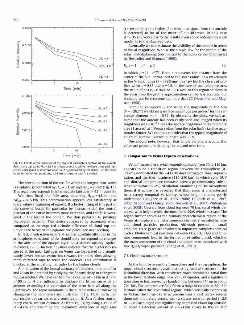
We then fitted the Pole area, obtaining Hpole = 4.8 km andDrpole = 38.5 km. This determination appears less satisfactory atlow f values (beginning of egress). If a better fitting of this part ofthe curve is forced (in particular by increasing Dr) the centralplateau of the curve becomes more extended, and the fit is wors-ened in the rest of the domain. We thus preferred to privilegethe overall better fit. This choice appears to be reasonable whencompared to the expected altitude difference of cloud top andupper haze between the equator and poles (see next section).

In fact, if refraction occurs at similar absolute altitudes in theatmosphere, variations of Dr should only correspond to changesin the altitude of the opaque layer, i.e. a slanted opacity (opticalthickness) s ! 1. Our best fit values indicate that the higher flux re-ceived at the polar latitudes on Venus can be related to a signifi-cantly lower aerosol extinction towards the poles, thus allowingmore refracted rays to reach the observer. This contribution isblocked at the equatorial latitudes by the higher clouds.

An indication of the formal accuracy of the determination of Drand H can be obtained by studying the fit sensitivity to changes inthe parameters. We have verified that a change of !3 km in Dr and!100 m in H are sufficient to displace the fitting curve of anamount exceeding the extension of the error bars all along thelightcurves. The rapid variations in the aureole behavior followingchanges in the parameters are illustrated in Fig. 17. In particular,our results appear extremely sensitive on H. As a further consis-tency check, we can estimate Dr from Eq. (3) by using a value ofH ! 4 km and assuming the maximum deviation of light rays

(corresponding to a highest f at which the signal from the aureoleis detected) to be of the order of x = 40 arcsec. In this caseDr ! 35 km, very close to the results given above obtained by a fullmodel fit to the observed data.

Eventually we can estimate the visibility of the aureole in termsof visual magnitude. We use the simple law for the profile of thesolar limb darkening (normalized to the Sun’s center brightness)by Hestroffer and Magnan (1998):

I'l( & 1$ u'1$ la( '7(

in which l = (1 $ r2)0.5. Here, r represents the distance from thecenter of the Sun, normalized to the solar radius. At a wavelengthin the V-band range (k = 579.9 nm) this law fits the observed pro-files when u = 0.85 and a = 0.8. In the case of our reference areathe value of r is rv = 0.969, so Iv = 0.428. In this region so close tothe solar limb the profile approximation can be less accurate, butit should not be erroneous by more than 2% (Hestroffer and Mag-nan, 1998).

From the computed Iv and using the magnitude of the Sun(V = $26.71) we obtain a surface magnitude per arcsec2 for the ref-erence element mv = $10.87. By observing the plots, we can as-sume that the aureole has been easily seen and imaged when itsbrightness was !10$2 times the surface brightness of the referencearea (1 arcsec2 at 1 Venus radius from the solar limb), i.e. five mag-nitudes fainter. We can thus consider that the typical magnitude ofan arc of aureole 1 arcsec in length was $5.9.

One should note, however, that ample variations around thisvalue are present, both along the arc and over time.

7. Comparison to Venus Express observations

Venus’ mesosphere, which extends typically from 70 to 110 km,appears to be a transition region between the troposphere (0–70 km), dominated by the !4 Earth days retrograde zonal superro-tation, and the thermosphere (110–250 km) in which solar EUVand diurnal temperature contrasts drive a predominantly subso-lar-to-antisolar (SS–AS) circulation. Monitoring of the mesophericthermal structure has revealed that this region is characterizedby a strong temporal variability, whose origin remains poorlyunderstood (Bougher et al., 1997, 2006; Lellouch et al., 1997,2008; Sandor and Clancy, 2005; Gurwell et al., 2007; Widemannet al., 2008). Upward from cloud top near 70 km, zonal winds de-crease with height while thermospheric SSAS winds increase. Theregion further serves as the primary photochemical region of theVenus atmosphere and heterogeneous chemistry revealed by hazeand cloud particles production. Although present in smallamounts, trace gases are involved in important complex chemicalcycles. Photochemical reactions between CO2, SO2, H2O and chlo-rine compounds lead to the formation of sulfuric acid, which isthe main component of the cloud and upper haze, associated withlow H2SO4 vapor pressure (Zhang et al., 2010).

7.1. Cloud and haze structure

At the limit between the troposphere and the mesosphere, theupper cloud structure reveals distinct dynamical structure in thelatitudinal direction, with convective, wave-dominated zonal flowin the lower latitude range near Venus’s equator, and a significanttransition to less convective banded flow between 45" up to about70"–80". The temperature field forms a bulge of cold air at 60"–80"latitude called the ‘‘cold collar region’’, which vertically extends upto 75 km. The torus-like structure encloses a vast vortex severalthousand kilometers across, with a slower rotation period (!2.5to !2.8 Earth days) and significantly depressed cloud top altitude,at about 62–65 km instead of 70–74 km closer to the equator

Fig. 17. Effects of the variation of the physical parameters controlling the aureoleflux. In the top panel, Heq = 4.8 km is kept constant, while the three simulated lightcurves correspond to different values of Dreq (indicated by the labels). On the otherhand, in the bottom panel Dreq = 38 km is constant and H is varied.

216 P. Tanga et al. / Icarus 218 (2012) 207–219

(Piccioni et al., 2007). The structure of the cloud tops is especiallypoorly investigated since it falls between the altitude rangessounded by solar/stellar occultations and that studied by descentprobes. Recent analysis has been performed on board Venus-Ex-press (Svedhem et al., 2007) based on depth of CO2 bands at1.6 lm measured by VIRTIS (Ignatiev et al., 2009), and CO + CO2

gaseous absorption in the 4.5–5 lm range using VIRTIS and VeRatemperature profiles (Lee et al., 2010) while Luz et al. (2011)brought the first extensive characterization of the vortex dynamicsand its precession motion. Although the absolute cloud top altitudepoleward and equatorward of the polar collar differs when apply-ing the two modeling techniques (63–69 km/74 ± 1 km in Ignatievet al., 2009; 62–64 km/ 66 km in Lee et al., 2010), their relative dif-ference is comparable (1–2 scale heights). The latitudinal extent ofthis polar depression matches well the brightest portion of theaureole observed southward of 65"–70" near the South polar limbin DOT telescope data (see Fig.8a of Ignatiev et al., 2009). Interest-ingly, similar agreement can be traced back to Russell’s drawings of1874 (see Link, 1969 and Fig. 1 of Pasachoff et al., 2011).

7.2. Haze aerosols

The Venus upper haze (70–90 km) was first evidenced by mea-surements from Pioneer Venus orbiter limb scans at 365 and690 nm at northern midlatitude. It is mainly composed of submi-cron sulfuric acid (H2SO4) aerosol particles with typical radii from0.1 to 0.3 lm (Lane and Opstbaum, 1983; Sato et al., 1996). Wil-quet et al. (2008) also present the first evidence for a bimodal par-ticles distribution, similar to the two modes in the upper clouds, atthe latitudes probed during the observation of solar and stellar occ-ultations by ESA’s Venus Express, with typical radii of mode-2 par-ticles between !0.4 and 1 lm. These measurements wereperformed close to the polar regions. From the results of Wilquetet al. (2008) the absorption at different wavelengths as a functionof the altitude can be deduced. In general, the absorption levels arefound to be 6 ± 1 km higher in the visible domain (SPICAV-IR at757 nm) than at 3 lm.

As an integrated aerosol optical depth !1 is measured a fewdensity scale heights above the cloud tops, we note that the slantedgeometry of the aureole must reach half occultation level r1/2 wellabove the upper haze. Quantitatively, the altitude of the aureole’shalf–occultation level in the polar region will be found by addingthe value of Drpole = 38.5 km to the altitude where aerosols slantedopacity s ! 1. Recent VEx/SOIR results (Wilquet et al., 2011, per-sonal communication) place that altitude at 73 ± 2 km in the3 lm band, to be further increased by 6 ± 1 km to retrieve its valuein the visible domain, as above. The final sum thus yieldsr1/2 ! 117.5 ± 4 km at the pole. Most recent VEx/SOIR results inte-grated over four years of observations (Wilquet et al., 2011) furtherindicate an altitude of longitudinally averaged, integrated aerosoloptical depth !1 increasing toward the equator, with an altitudeof 81 ± 2 km for latitudes between 35"S and 55"S. Therefore, asDreq = r1/2 $ rcut is significantly smaller than Drpole the resultingvalue of r1/2 at mid-latitude differ from our calculation in the polarregion by about two scale heights (Table 2). We can thus considerthat our results only show marginal latitudinal variation of the

altitude for the half-occultation level along the terminator,although in a region of important temperature variation whichneed to be independently assessed. The same SPICAV/SOIR resultsshow that, under reasonable assumptions, the refraction index atvisible wavelengths is fairly constant, thus confirming that the pro-cess is not a source of relevant chromatic effects in the aureole.

7.3. Temperature structure

Only scarce measurements of vertical temperature profiles havebeen performed above 100 km altitude, where temperature fields,especially in the polar region, as well as their time variability, arestill debated (see, e.g., Vandaele et al., 2008; Clancy et al., 2008,2011; Piccialli et al., 2008, 2011). Inverted equator-to-pole temper-ature gradient on isobaric surfaces above 75 km, were first re-ported by NASA’s Pioneer Venus Infrared Radiometer and radiooccultation measurements (Taylor et al., 1983; Newman et al.,1984), Venera-15 Fourier Spectrometry data (Zasova et al., 2006)and more recently ESA’s Venus Express, e.g. Grassi et al. (2008),Piccialli et al. (2008) using VIRTIS-M observations; Tellmannet al. (2009) based on VeRa radio occultations on board VEx. Thecollar region also divides the atmosphere vertically. Below the col-lar, the atmosphere cools with increasing latitude. Above, the tem-perature gradient is reversed, as diabatic heating or dynamicallycontrolled processes could be responsible for the observed struc-tures (Schubert et al., 1980; Tellmann et al., 2009). At the altitudeof the collar and closer to the poles, the atmosphere is almost iso-thermal and also much warmer than the surrounding areas. Verti-cal temperature profiles are fairly constant with altitude betweenaround 50 and 100 km, above which they begin to rise sharply inthe mesosphere, see e.g. Fig. 2 in Mueller-Wodarg et al. (2006).

Retrieving the temperature using the density scale heightshould be made with caution. The transition between stable andadiabatic regions is fairly smooth at equatorial latitudes, butabrupt at middle and polar latitudes (Tellmann et al., 2009). A sig-nificant vertical temperature gradient is a potential issue when try-ing to compare the density scale height to the temperature scaleheight (see the discussion related to Titan’s mesosphere refractiv-ity in Sicardy et al. (2006)). However, we consider the mid-occulta-tion level probed by the arc in the !115 km region (see Table 2) asisothermal. This is an acceptable hypothesis since the diurnal aver-age of dT/dz on the background atmosphere (Hedin et al., 1983) isnegligible, although significant local-time and daily variability hasbeen retrieved (Clancy et al., 2008, 2011; Sonnabend et al., 2008,2011). In particular, the elevated value of Tiso = 212 K at120.5 ± 4 km at 68"S is in agreement with high kinetic tempera-tures derived from heterodyne mid-infrared spectrum of non-LTEemission at terminator, see in particular Table 1 of Sonnabend etal. (2011). This result suggests a warmer or rapidly variable tem-perature condition in the altitude range.

7.4. Physical interpretation

In order to check the consistency of our results with the knownphysics of Venus atmosphere, we can compute the expected valueof the density scale height H at the altitude of the refracting layer.The temperature scale height is defined as H = kT(mg)$1, where k isthe Boltzmann’s constant, while T, m and g respectively representtemperature, molecular mass and gravitational acceleration atthe altitude considered. As discussed above, we consider a locallyisothermal atmosphere. For our computation we derive the valueof g as a function of altitude. We derived an altitude for the opaquelayer from SOIR aerosol transmittance measurements near 3 lm(Wilquet et al., 2011, Wilquet, personal communication), andadded 6 ± 1 km for transferring to the visible domain. We thenadopt the model by Hedin et al. (1983) describing the atmospheric

Table 2Results of modelling and retrieved half-light altitude r1/2, scale height H (in km) andtemperature along the Lomonosov’s arc, assuming a locally isothermal atmosphere.Explanations of symbols in the text. Tiso =m(z)g(z)H/k. Tmod (K) from Hedin et al.(1983).

Point Lat. Dr H rcut r1/2 Tiso (K) Tmod (K)

A 68"S 38.5 ± 3 4.8 ± 0.1 76 ± 2 120.5 ± 4 212 138–190B 45"S 26.0 ± 3 3.1 ± 0.1 81 ± 2 113.0 ± 4 137 143–185

P. Tanga et al. / Icarus 218 (2012) 207–219 217

structure on Venus at noon and midnight, around the equator. Weconsider that an appropriate temperature estimation can be ob-tained by averaging the two profiles. Differences may be present,since we observe directly at the terminator, but the temperaturedata by SOIR obtained at a similar geometry (Mahieux et al.,2010) do not show significant discrepancies relative to the model.CO2 is the dominant gas on the dayside below 160 km and on thenightside below 140 km, replaced at higher altitudes by O. Meanmolecular mass remains close to 44 a.m.u. below 130 km, whereCO2 dominates, and decreases towards higher altitudes (Hedinet al., 1983; Mueller-Wodarg et al., 2006). Although day–night dif-ferences in composition are substantial, we also may consider lon-gitudinally averaged values at the altitude considered. Concerningm, since the layer is in the heterosphere, a decrease due to fraction-ation has to be taken into account, due to the decrease in CO2 rel-ative to other components, in particular atomic oxygen O,molecular nitrogen N2 and He. As a result, at 120 km we use anaverage molecular mass of 42.9, and a day-night longitudinal aver-age T = 164 K, obtaining H = 3.7 km. An equal value is obtained at115 km. Both are in remarkable agreement with the average oneobtained from the aureole measurements, H = 3.95 km (see Table2). Finally, we noted that our results only show marginal latitudi-nal variation of 1–2 scale heights for the altitude for the half–occultation level along the terminator, near 117 km.

8. Conclusions

Our results represent the first successful model of the aureole ofVenus, observed during solar transits. We are able to reproduce themain features of the lower mesosphere observational constraints:longitudinally averaged thermal structure near 117 km, slantedopacity of aerosols and their meridional variation, with consistentphysical parameters.

The results obtainedby this first set ofmeasurements are encour-aging and suggest that more accurate planning will produce moreprecise data. Improvements are also possible concerning the refrac-tion model, which could be completed by a more realistic, gradualtransition from transparency to absorption at the cloud deck levelbased onmost recent results on the latitudinal distribution of upperhaze aerosols. Also, the contribution of scattered light in addition torefracted light could be included. In fact, the absorption curves inWilquetet al. (2008)Fig. 3 arewavelengthdependent, i.e. theopaquelayer altitude inourmodel canbe functionof the color. As a result theaureole should not be perfectly ‘‘gray’’, suggesting that future obser-vations capable of accurate multicolor photometry should investi-gate this possibility.Even a gray absorption would cause the solarflux in the aureole to look dimmer than without aerosols, whichwould be wrongly interpreted as a drop in scale height, i.e. in localtemperature at tangent point altitude, in the inversion code.

In the two hemispheres, the cold collar temperature structureand the polar regions are very similar (Tellmann et al., 2009), sothe latitudinal variations obtained for the 2004 transit around theSouth polar region might tentatively apply to the North polar datawe expect to acquire in June 2012. Recent interpretations also attesta general N–S symmetry in the latitudinal variation of aerosolsextinction (Wilquet et al., 2011). Given the difference in brightnessbetween the arc and the solar photosphere, accuratemeasurementsof this phenomena are challenging. The degree of turbulence, themagnification, the amount of light scattering in the optics are allelements that contribute in determining the effective visibility ofthe aureole in a given instrument, and the accuracy of the measure-ments. The transit of June 2012 will be our last opportunity forobserving the aureole using this spatially resolved technique, untilthe next pair of transits of Venus, which will be in the ascendingnode, on 11 December 2117 and 8 December 2125.

Acknowledgments

We thank the referees for useful comments on the manuscript,M. Frassati and Unione Astrofili Italiani for the use of the drawingreproduced in Fig. 2. We also thank Valérie Wilquet, Ann-CarineVandaele and Arnaud Mahieux of the Belgium Institute for SpaceAeronomy for sharing their work in progress on the longitudinallyaveraged optical extinction of mesospheric aerosols on Venus. R.Hammerschlag (Dutch Open Telescope, La Palma) provided valu-able help and comments.

References

Baum, W.A., Code, A.D., 1953. A photometric observation of the occultation of rArietis by Jupiter. Astron. J. 58, 108–112.

Bettonvil, F.C.M., Hammerschlag, R.H., Sutterlin, P., Jagers, A.P.L., Rutten, R.J., 2003.Multi-wavelength imaging system for the Dutch Open Telescope. In: Keil, S.L,Avakyan, S.V. (Eds.), Innovative Telescopes and Instrumentation for SolarAstrophysics. Proc. SPIE 4853, pp. 306–317.

Bougher, S.W., Alexander, M.J., Mayr, H.G., 1997. Upper atmosphere dynamics:Global circulation and gravity waves. In: Bougher, S.W., Hunten, D.M., Phillips,R.J. (Eds.), Venus II. University of Arizona Press, Tucson, pp. 259–291.

Bouguer, S.W., Rafkin, S., Drossart, P., 2006. Dynamics of the Venus upperatmosphere: Outstanding problems and new constraints expected from VenusExpress. Planet. Space Sci. 54, 1371–1380.

Clancy, R.T., Sandor, B.J., Moriarty-Schieven, G.H., 2008. Venus upper atmosphericCO, temperature, and winds across the afternoon/evening terminator from June2007 JCMT sub-millimeter line observations. Planet. Space Sci. 56, 1344–1354.

Clancy, R.T., Sandor, B.J., Moriarty-Schieven, G., 2011. Thermal structure and COdistribution for the Venus mesosphere/lower thermosphere: 2001–2009inferior conjunction sub-millimeter CO absorption line observations. Icarus, inpress. doi:10.1016/j.icarus.2011.05.032.

Dollfus, A., Maurice, E., 1965. Étude de l’allongement des cornes du croissant deVénus. C.R. Acad. Sci. 260, 427–430.

Edson, J.B., 1963. The twilight zone of Venus. In: Kopal, Z. (Ed.), Advances inAstronomy and Astrophysics, vol. 2. Cambridge Scientific Publishers, London,New York, pp. 17–31.

Grassi et al., 2008. Retrieval of air temperature profiles in the venusian mesospherefrom VIRTIS-M data: Description and validation of algorithms. J. Geophys. Res.113, E00B09.

Gurwell, M.A., Melnick, G.J., Tolls, V., Bergin, E.A., Patten, B.M., 2007. SWASobservations of water vapor in the Venus mesosphere. Icarus 188, 288–304.

Hedin, A.E., Niemann, H.B., Kasprzak, W.T., 1983. Global empirical model of theVenus thermosphere. J. Geophys. Res. 88 (A1), 73–83.

Hestroffer, D., Magnan, C., 1998. Wavelength dependency of the solar limbdarkening. Astron. Astrophys. 333, 338–342.

Howell, S.B., 1989. Two-dimensional aperture photometry: Signal-to-noise ratio ofpoint-source observations and optimal data-extraction techniques. Publ.Astron. Soc. Pacific 101, 616–622.

Ignatiev, N.I. et al., 2009. Altimetry of the Venus cloud tops from the Venus Expressobservations. J. Geophys. Res. 114, E00B43.

Lane, W.A., Opstbaum, R., 1983. High altitude Venus haze from Pioneer Venus limbscans. Icarus 54, 48–58.

Lee, Y.J. et al., 2010. Vertical structure of the Venus cloud top from the VeRa andVIRTIS observations onboard Venus Express. EGU General Assembly 2010, 12,EGU2010-11522-1 (abstract).

Lellouch, E., Clancy, T., Crisp, D., Kliore, A.J., Titov, D., Bougher, S.W., 1997.Monitoring of mesospheric structure and dynamics. In: Bougher, S.W.,Hunten, D.M., Phillips, R.J. (Eds.), Venus II. University of Arizona Press, Tucson,pp. 295–324.

Lellouch, E., Paubert, G., Moreno, R., Moullet, A., 2008. Monitoring Venus’mesospheric winds in support of Venus Express: IRAM 30-m and APEXobservations. Planet. Space Sci. 56, 1355–1367.

Link, F., 1969. Eclipse Phenomena in Astronomy. Springer-Verlag, Berlin.Luz, D. et al., 2011. Venus southern polar vortex reveals processing circulation.

Science 332 (6029), 577.Mahieux, A. et al., 2010. Densities and temperatures in the Venus mesosphere and

lower thermosphere retrieved from SOIR on board Venus Express: Retrievaltechnique. J. Geophys. Res. (Planets) 115, E14, E1201.

Marov, M.Y., 2005. Mikhail Lomonosov and the discovery of the atmosphere ofVenus during the 1761 transit. In: Kurtz, D.W., Bromage, G.E. (Eds.), Transits ofVenus: New Views of the Solar System and Galaxy, IAU Colloq. 196. CambridgeUniversity Press, pp. 209–219.

Mueller-Wodarg, I.C.F., Forbes, J.M., Keating, G.M., 2006. The thermosphere of Venusand its exploration by a Venus Express Accelerometer Experiment. Planet. SpaceSci. 54, 1415–1424.

Newman, M., Schubert, G., Kliore, A.J., Patel, I.R., 1984. Zonal winds in the middleatmosphere of Venus from Pioneer Venus radio occultation data. J. Atmos. Sci.41, 1901–1913.

Pasachoff, J.M., Sheehan, 2012. Lomonosov, the discovery of Venus’s atmosphere,and eighteenth-century transits of Venus. J. History Heritage Astron., submittedfor publication.

218 P. Tanga et al. / Icarus 218 (2012) 207–219

Pasachoff, J.M., Schneider, G., Widemann, T., 2011. High-resolution satellite imagingof the 2004 transit of Venus and asymmetries in the Cytherean atmosphere.Astron. J. 141, 112.

Piccialli, A. et al., 2008. Cyclostrophic winds from the Visible and Infrared ThermalImaging Spectrometer temperature sounding: A preliminary analysis. J.Geophys. Res. 113, E00B11.

Piccialli, A., Tellmann, S., Titov, D.V., Limaye, S.S., Khatuntsev, I.V., Pätzold, M.,Häusler, B., 2011. Dynamical properties of the Venus mesosphere from theradio-occultation experiment VeRa onboard Venus Express. Icarus, in press.doi:10.1016/j.icarus.2011.07.016.

Piccioni, G. et al., 2007. South-polar features on Venus similar to those near thenorth pole. Nature 450, 637–640.

Russell, H.N., 1899. The atmosphere of Venus. Astrophys. J. 9, 284–299.Rutten, R.J., Hammerschlag, R.H., Bettonvil, F.C.M., Sutterlin, P., de Wijn, A.G., 2004.

DOT tomography of the solar atmosphere. Astron. Astrophys. 413, 1183–1189.Sandor, B.J., Clancy, R.T., 2005. Water vapor variations in the Venus mesosphere

from microwave spectra. Icarus 177, 129–143.Sato, M., Travis, L.D., Kawabata, K., 1996. Photopolarimetry analysis of the Venus

atmosphere in polar regions. Icarus 124, 569–585.Schroeter, J.H., 1791. Selenotopographische Fragmente zur Genauern Kenntniss der

Mondfläche, ihrer Erlittenen Veränderungen und zeichnungen, UniversitätsGöttingen.

Schubert, G. et al., 1980. Structure and circulation of the Venus atmosphere. J.Geophys. Res. 85, 8007–8025.

Sicardy, B. et al., 2006. The two Titan stellar occultations of 14 November 2003. J.Geophys. Res. 111, E11S91.

Sonnabend, G., Sornig, M., Scheider, R., Kostiuk, T., Delgado, J., 2008. Temperaturesin Venus upper atmosphere from mid-infrared heterodyne spectroscopy of CO2

around 10 lm wavelength. Planet. Space Sci. 56 (10), 1407–1413.Sonnabend, G., Krötz, P., Schmülling, F., Kostiuk, T., Goldstein, J., Sornig, M., Stupar,

D., Livengood, T., Hewagama, T., Fast, K., Mahieux, A., 2011. Thermospheric/mesospheric temperatures on Venus: Results from ground-based high-

resolution spectroscopy of CO2 in 1990/1991 and comparison to results from2009 and between other techniques. Icarus, in press. doi:10.1016/j.icarus.2011.07.015.

Svedhem, H., Titov, D.V., Taylor, F.W., Witasse, O., 2007. Venus as a more Earth-likeplanet. Nature 450, 629–632.

Taylor, F.W., Hunten, D.M., Ksanfomality, L.V., 1983. The thermal balance of themiddle and upper atmosphere of Venus. In: Hunten, D.M., Colin, L., Donahue,T.M., Moroz, V.I. (Eds.), Venus. University of Arizona Press, Tucson, AZ, pp. 650–680.

Tellmann, S., Paetzold, M., Hausler, B., Bird, M.K., Tyler, G.L., 2009. Structure ofVenus neutral atmosphere as observed by the Radio Science experiment VeRaon Venus Express. J. Geophys. Res. (Planets) 114, E00B36.

Vandaele, A.C. et al., 2008. J. Geophys. Res. (Planets) 113, E00B23.Widemann, T., Lellouch, E., Donati, J.-F., 2008. Venus Doppler winds at cloud tops

observed with ESPaDOnS at CFHT. Planet. Space Sci. 56 (10), 1320–1334.Widemann, T. et al., 2009. Titania’s radius and an upper limit on its atmosphere

from the September 8, 2001 stellar occultation. Icarus 199 (2), 458–476.Wilquet, V. et al., 2008. Preliminary characterization of the upper haze by SPICAV/

SOIR solar occultation in UV to mid-IR onboard Venus Express. J. Geophys. Res.(Planets) 114, E00B42.

Wilquet, V., Drummond, R., Mahieux, A., Robert, S., Vandaele, A.C., Bertaux J.L.,2011b. Optical extinction due to aerosols in the upper haze of Venus: Four yearsof SOIR/VEX observations from 2006 to 2010. Icarus, in press. doi:10.1016/j.icarus.2011.11.002.

Yuen, H.K., Illingworth, J., Kittler, J., 1989. Detecting partially occluded ellipses usingthe Hough transform. Image Vis. Comput. 7, 31–37.

Zasova, L.V., Moroz, V.I., Linkin, V.M., Khatuntsev, I.V., Maiorov, B.S., 2006. Structureof the venusian atmosphere from surface up to 100 km. Cosmic Res. Engl.Transl. 44 (4), 364–383.

Zhang, X., Liang, M., Montmessin, F., Bertaux, J.-L., Parkinson, Ch., Young, Y.L., 2010.Photolysis of sulphuric acid as the source of sulphur oxides in the mesosphereof Venus. Nat. Geosci. Lett. 3, 834–837.

P. Tanga et al. / Icarus 218 (2012) 207–219 219