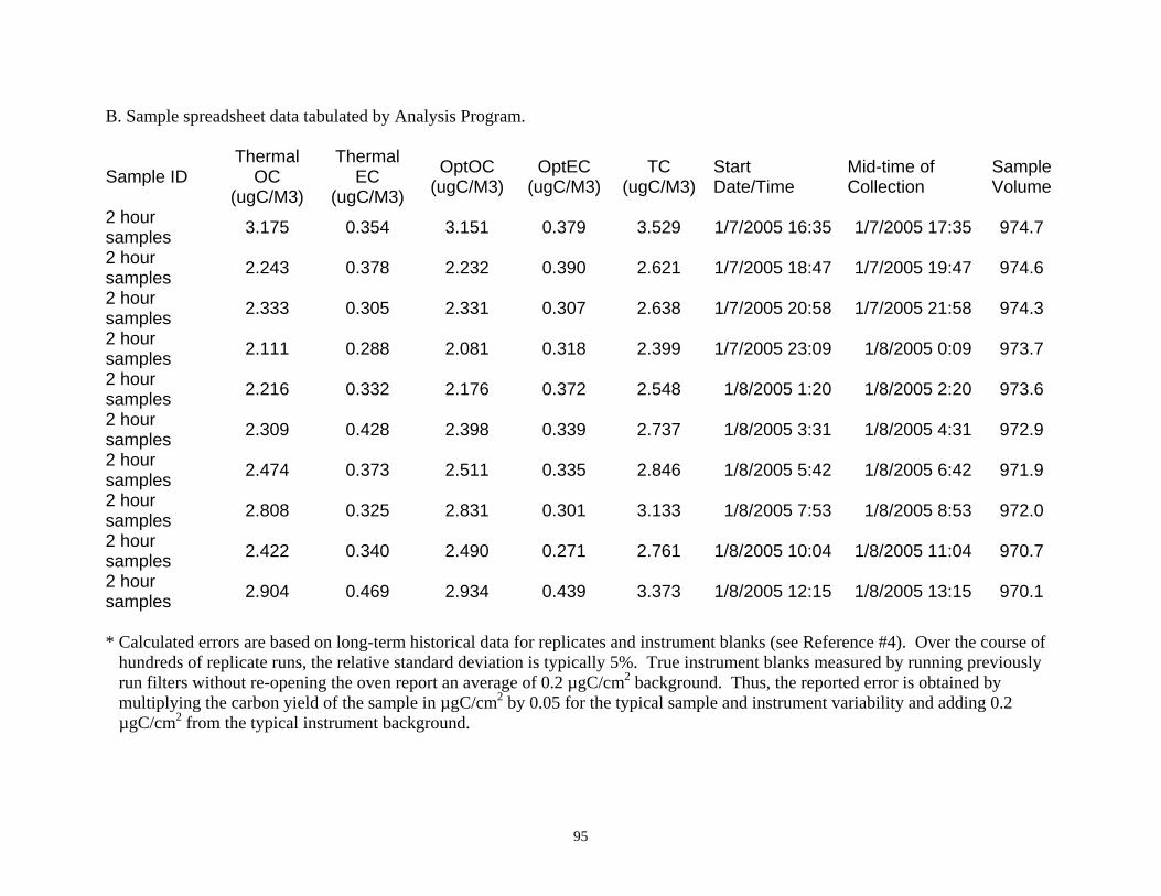
Sunset Laboratory Inc. S S E EM MI I - - C CO ON NT TI I N NU UO OU US S O OC C E E C C C CA AR RB BO ON N A AE ER RO OS S O OL L A AN NA AL L Y YZ ZE ER R A GUIDE TO RUNNING AND MAINTAINING THE SUNSET LABORAORY SEMI-CONTINUOUS OCEC ANALYSER Sunset Laboratory Inc. 10180 SW Nimbus Ave. Suite J-5 Portland, OR 97223
Transcript
Sunset Laboratory Inc.
SSEEMMII--CCOONNTTIINNUUOOUUSS OOCCEECC
CCAARRBBOONN AAEERROOSSOOLL AANNAALLYYZZEERR
A GUIDE TO RUNNING AND MAINTAINING THE SUNSET LABORAORY
IInnttrroodduuccttiioonn Congratulations; you have purchased the finest Semi-Continuous OCEC Carbon Aerosol analysis instrument on the market today. Sunset Laboratory Inc. has been a leader in the development of the OCEC aerosol analyzer since the early 1980’s and has offered commercial laboratory instruments for more than 12 years. Sunset Laboratory has performed much of the instrument development leading to the current state of thermal/optical OC/EC measurement techniques. In addition, Sunset Laboratory has performed literally thousands of OC/EC analyses ranging from mining samples to ambient atmospheric samples. The Semi-Continuous OCEC Analyzer is the latest addition to our growing line of products and services in the field of carbon aerosol analysis. TThheeoorryy ooff AAnnaallyyssiiss OOppeerraattiioonn Sunset Laboratory’s Semi-Continuous OCEC instrument has been developed as a field deployable alternative to integrated filter collection with subsequent laboratory analysis. This instrument can provide time-resolved OCEC analyses on a semi-continuous basis with OCEC (organic and elemental carbon) results comparable to the recognized NIOSH Method 5040. As currently performed, a quartz filter punch is mounted in the instrument, then samples are collected for the desired time period. Once the collection is complete, the oven is purged with helium, a stepped-temperature ramp increases the oven temperature to 850 °C, thermally desorbing organic compounds and pyrolysis products into a manganese dioxide (MnO2) oxidizing oven. As the carbon fragments flow through the MnO2 oven, they are quantitatively converted to CO2 gas. The CO2 is swept out of the oxidizing oven with the helium stream and measured directly by a self-contained non-dispersive infrared (NDIR) detector system. A second temperature ramp is then initiated in an oxidizing gas stream and any elemental carbon is oxidized off the filter and into the oxidizing oven and NDIR. The elemental carbon is then detected in the same manner as the organic carbon. Three characteristic components of this method are important in the strength of the analysis. The first of these is the optical detection and correction for elemental carbon. Elemental carbon is naturally present in many of these samples from some combustion source such as a diesel exhaust. This black material is a very strong absorber of light, and almost always the only absorber in the red light region. In addition to this elemental carbon in the sample, elemental carbon can be formed from some charring of the organic carbon fraction of the sample as it is pyrolyzed during the initial temperature ramp. This can begin occurring as low as 300 °C depending on the organic components on the filter. This charring of organic carbon could result in an artificially low measurement of the organic carbon and a higher than actual measurement for the original elemental carbon if no correction is made. The Sunset Laboratory thermal/optical method uses the high light absorbance characteristic of elemental carbon to correct for the pyrolysis-induced error. This is done by incorporating a tuned diode laser (red 660 nm), focused through the sample chamber
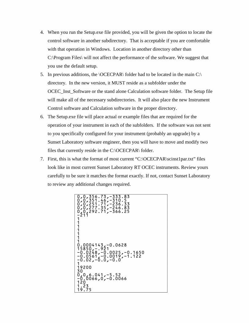
such that the laser beam passes through the mounted filter in the sample oven. Initial absorbance of the modulated laser beam is recorded. As the oven ramp proceeds, the laser absorbance is monitored continuously by the data system. Any charring of the organic carbon results in an increase in absorbance of the laser. After the initial temperature ramp, when the helium is switched to a He/O2 mixture, all of the elemental carbon is oxidized off and the laser absorbance is reduced to the background level. When the resulting NDIR data are reviewed with an overlay of the laser absorbance, the point in the second phase oxidizing ramp at which the laser absorbance equals the initial laser absorbance is the split point. Any elemental carbon detected, before this point, is said to have had been formed pyrolytically by charring of the organic carbon. This carbon is subtracted from the elemental carbon area observed during the oxidizing phase of the analysis and is assigned as organic carbon. The primary assumption, for this correction, is that the particulate bound elemental carbons and the pyrolytically formed elemental carbons have the same absorption coefficient. Carefully prepared standard samples suggest that this correction is satisfactory. The second component of the analysis is the use of a sensitive, linear detector for this measurement. Historically, this has been a flame ionization detector. Recently Sunset Laboratory has introduced is own self-contained flow-through NDIR system. This unit provides results comparable to FID at typical ambient levels. It is a RISC-processor controlled pseudo-dual beam instrument with temperature stabilized source and a linearized signal output. Calibrations are constant for up to a year. NDIR eliminates the requirement for air or hydrogen at the field site significantly reducing the requirements for consumable gases. The conversion to NDIR of the Sunset Laboratory field analyzer represents a significant step forward in reliability and reduced complexity. The third important component of the measurement system is the incorporation of a fixed volume loop used to inject an external standard at the end of every analysis. This external standard data is incorporated into every data package and is used along with the known carbon concentration in the loop to calculate the analytical results. By having every sample correlated to an external standard injection with each analysis, small variations in instrument performance normalized out resulting in a very stable, repeatable analytical method.
Safety The purpose of this section is to provide information on the safety precautions that should be taken around the instrument. Types of safety issues: 1. Laser 2. High voltage wiring 3. Weight 4. Temperature Laser The Sunset Laboratory Semi-Continuous OCEC Carbon Aerosol Analyzer uses a laser diode for the transmission light source during the sample collection and analysis. As such, a report on its configuration has been filed with the Food and Drug Administration; Center for Devices and Radiological Health (CDRH). Caution: use of control, adjustments, or performance of procedures other than specified herein may result in hazardous radiation exposure. The Sunset Laboratory Semi-Continuous OCEC Carbon Aerosol Analyzer is classified as a Class 1 Laser Product, which means that there is no laser radiation exposure during operation and maintenance. The interlocked laser system is embedded in the instrument with a closed optical system. The interlock-protected laser shroud covers the laser aperture/photodetector preventing any direct or collateral exposure to the laser system. The attached photodetector head also serves as an additional non-interlocked protective housing covering the laser aperture and sealing the entire system. In order to gain access to the photodetector head to change filters, the operator must remove the protective laser shroud. When this operation is performed, it actuates the interlock shutting down the laser via an electromechanical switch. Once the shroud is removed (and the laser disabled), the operator can safely remove the photodetector head and change the filter. Secondary protection is provided by the instrument housing, which is secured by a series of screws. Some weakly scattered laser light may be indirectly observed during operation but is not measurable above background lighting. The source laser diode is rated as a Class IIIb product as a standalone unit and emits sufficient optical power to constitute a possible hazard to the human eye if directly exposed to the beam. Therefore, the present Semi-Continuous OCEC analyzer optical system has no user serviceable parts. All repairs and services must be performed by one of Sunset Laboratory’s trained technicians. As a Class I Laser Product, no laser hazard warnings are required on the exterior of the instrument. However, when the maintenance access panel is opened, the first of several laser radiation warning labels are observed. This is located on the laser shroud/interlock
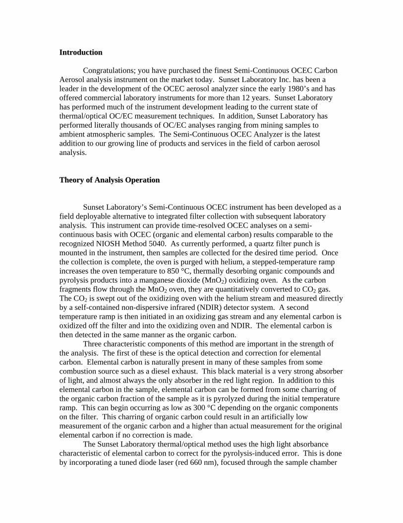
housing. It warns that laser radiation may be present if the shroud is removed and the interlock is defeated. This is shown below:
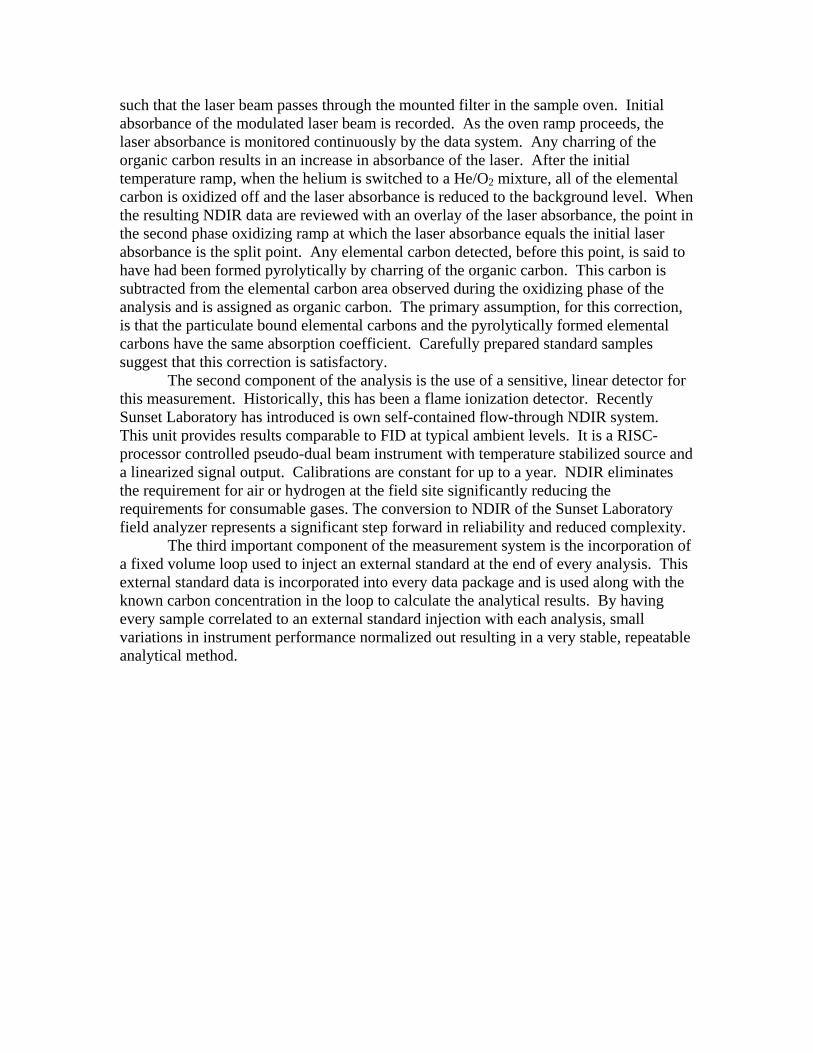
The interlock system can only be defeated by the use of a special override key. The key will only be provided to Sunset Laboratory- trained Service Technicians. No keys will be provided to the user. When the laser shroud is removed, two more labels may be observed. The first label is on the aluminum photodetector head, mounted over the end of the optical path, which serves as a non-interlocked protective housing and source detector. This effectively seals off the laser radiation system preventing exposure as long as the photodetector remains installed. The protective housing label, shown below; indicates the type and power of the laser which may be present if the photodetector head is removed with the interlock system defeated.
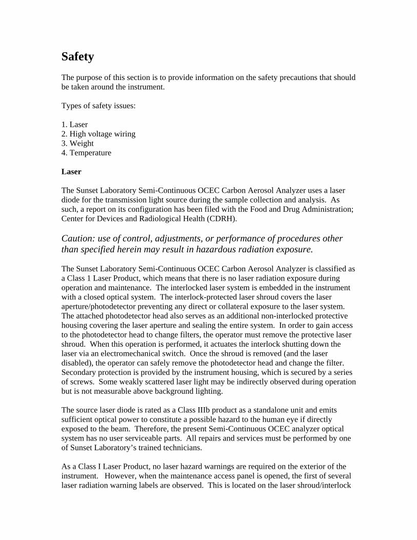
Should the photodetector (and thus, the associated warning label) be removed, a second warning label located on the mounting plate indicates the open laser aperture. This label also indicates the type and power of the laser diode and warns that direct exposure is possible at the open aperture if the system is opened and the interlock is defeated. This label is reproduced below:
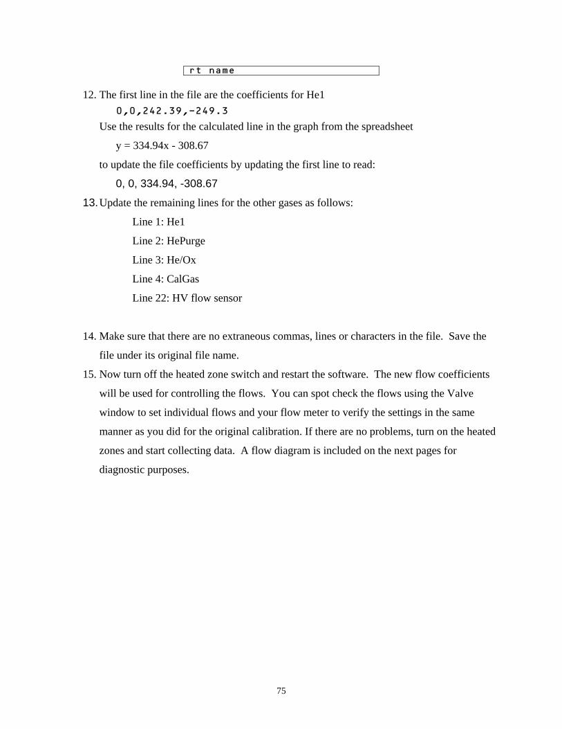
No hazardous exposure is possible under normal operating conditions and/or maintenance procedures. The protective interlock system shall only be defeated by a trained service technician using prescribed procedures from the factory. A fourth label, located on the outside of the case on the back, serves as the product identification and product certification as required under 21 CFR 1010.2 and 1010.3. This label, shown below also the instrument serial number, manufacturing completion date and place of manufacture.
Sunset Laboratory Inc. certifies that this product conforms to all applicable provisions of 21 CFR Subchapter J in effect as of the Date of Manufacture. Any effort to defeat the interlock system of service the laser system in this instrument by anyone other than a trained service technician could result in a dangerous exposure to laser radiation. Furthermore, any effort to service, alter or modify the optical system by the user may void the warranty and absolves Sunset Laboratory Inc. of any liability regarding exposure to laser radiation.
High Voltage Wiring Sunset Laboratory Inc. uses either 115V or 230V AC electric power to operate its Semi-Continuous OCEC instruments. In general, the AC wiring is isolated to the closed area under the instrument cabinet and properly labeled with a “Danger High Voltage” label. Any repair work in this area should only be performed by a trained technician. Every reasonable effort has been made to isolate the AC power from the user. However, no service work should ever be performed on the instrument unless the AC power cord has been unplugged from the AC power inlet. High Temperatures In general, the analyzer uses high temperature to analyze for the carbon content of the aerosol samples. Heated zones are marked in bright red warning labels. Avoid contact with these areas. The ovens should be allowed to cool completely before beginning any maintenance or repair work. Weight The instrument weighs approximately 30 pounds. Use caution when lifting and moving the device to avoid causing injury.
I Health and Safety Warnings
The Sunset Laboratory Thermal/Optical Carbon Analyzer uses high temperatures (up to 870C) and laser radiation to perform the required steps in this analytical procedure. Under normal operation, the analyst is protected from exposure to these energy sources. However, during repair or trouble shooting, when the instrument cover is removed, the analyst must take the following precautions:
a) Before attempting any repairs, turn off the power and wait for all heated zones to cool.
b) For most repair work, unplug power to the ovens and avoid contact with any power sources in the oven cabinet.
c) Although the laser source has an interlock protection system, if the interlock is overridden, direct exposure to the laser can occur under certain conditions. Do not look directly at the laser source as permanent eye damage can occur.
d) Use caution when handling all support gas cylinders and regulators. Always have cylinders properly chained to a safety rack.
e) Always wear Safety Glasses and a dust mask when removing and installing the ceramic insulation in the ovens during the installation of heating coils. The insulation does not contain asbestos, however, safe handling of the high
temperature insulation should be considered as a good precaution against unknown health hazards.
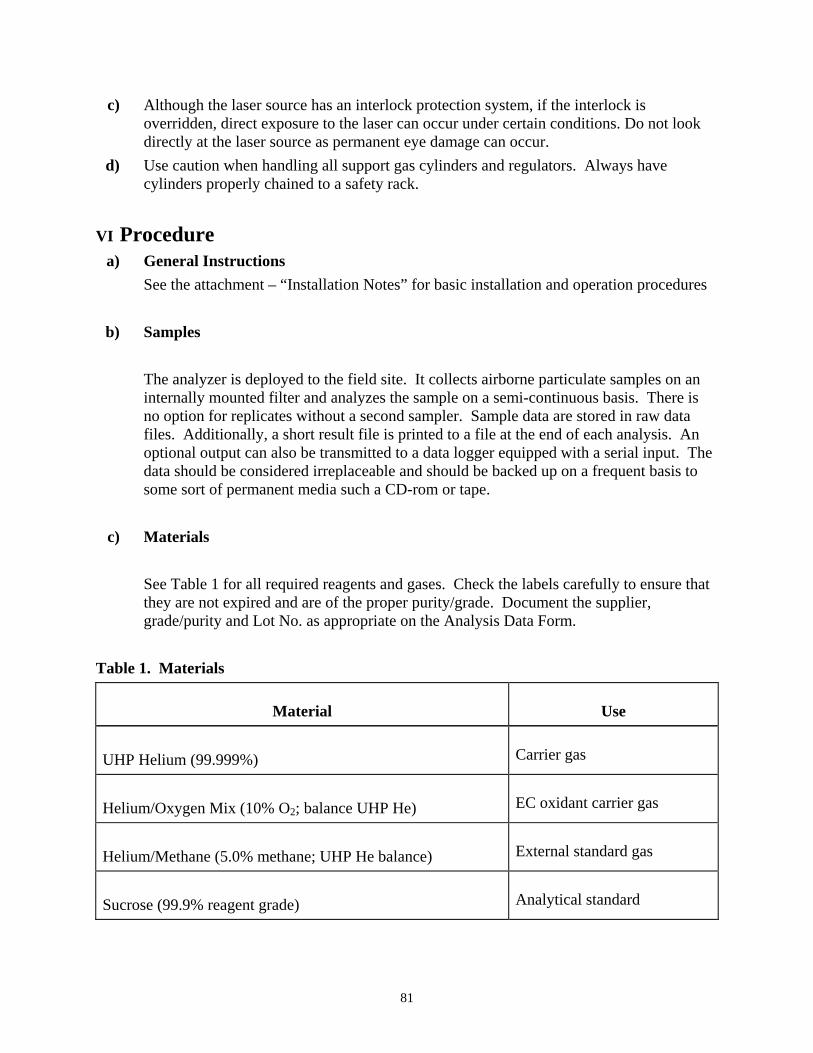
1. PPoowweerr – The Sunset Laboratory Semi-Continuous OCEC Instrument requires a separately fused 120/240V AC power receptacle (15 Amp). The single power line is sufficient to power all phases of the instrument operation. Separate switches are provided to isolate the heated zones from the CPU and blower. This is necessary for testing and troubleshooting.
2. SSuuppppoorrtt GGaasseess – there are five support gases (to be) supplied by the customer along with regulators. These are required to be at the site prior to setting up an installation.
a. HHeelliiuumm –the main carrier gas is helium. This should be at least 99.999% ultra high purity grade with low moisture, hydrocarbon, carbon dioxide, carbon monoxide and oxygen background. (a GC quality oxygen trap is also recommended for the regulator outlet). CO2 and hydrocarbon content should be less that 1 ppm.
b. HHeelliiuumm//ooxxyyggeenn – this is a custom blend gas with 10% oxygen and 90% helium balance. It should be ordered with sufficient lead time by the customer to allow for blending by the gas vendor (typically 2-4 weeks). The helium should be the same quality as the main source helium and the oxygen should be 99.999% or better with low moisture, hydrocarbon, carbon dioxide, carbon monoxide and hydrocarbon background. (CO2 and hydrocarbon levels should be less than 1 ppm).
c. HHeelliiuumm//mmeetthhaannee- this is also a custom blend with 5.0% methane and 95% helium balance. Again, this should be ordered with sufficient lead time by the customer to allow for blending by the gas vendor (typically 2-4 weeks). The helium should be the same quality as the main source helium and the methane should be research grade or better with low moisture background.
3. CCoommppuutteerr – Sunset Laboratory will typically supply a laptop computer for
field operation of the semi-continuous analyzer. It will come with the operating software pre-installed. Training on the operation and use of the software will be provided at the time of initial installation. An un-interruptible power supply (UPS) for the computer (but not the instrument) is also highly recommended to maintain the integrity of the system in the event of a power outage. User supplied computers should be at least 500 MHz Pentium II or better with 10 GB hard drive, 256 M memory, 2 serial ports and preferably a R/W CD drive. Laptop computers are preferred for field deployment because they are small and offer temporary battery operation in the event of a power outage. The 2 serial ports are mandatory for the operation of the instrument. Many laptops today offer only 1 serial port (and some with no serial ports). The best solution to this is to obtain a PCMCIA card based serial port(s). These devices are far more reliable (for now) than the USB port serial devices.
Check with Sunset Laboratory for detailed specification and recommendations.
4. Sampling System – The Sunset Labs Semi-Continuous analyzer is equipped with a 3/8” stainless steel ball valve port located on the back of the unit as the sample inlet. Samples are pulled through the ball valve, across the mounted quartz filter, through a mass flow meter and out to the remote sample pump. Initiation of sampling is facilitated through a remote controlled power cord. This can be used to turn on a pump or actuate a 120 VAC solenoid valve to start and stop sample collection. A ballast tank is also provided to prevent filter disruption at the initiation of sampling. Because of the wide range of possible samples and customer sampling requirements, no additional sample introduction components are provided with the basic instrument package. The following components are suggested (or required) to complete the initial installation.
a. Pump (required) – an oil-less carbon vane pump with a minimum capacity of 24 liters/min at –15 psi vacuum.
b. ¼” Tubing (required) – sample vacuum ports on the rear of the instrument are ¼” Swageloc tube ports. The customer shall provide sufficient Teflon or nylon tubing as required to reach the ballast tank and pump.
c. Organic denuder (optional) – organic denuders have been shown to reduce the effects of vapor phase organic adsorption to the cleaned quarts filter. These are currently available as multiple concentric tube and parallel plate devices. Sunset Labs can provide additional advice towards the proper sizing and acquisition of these devices. Sunset Laboratory can provide a parallel plate organic denuder at additional cost.
d. PM (particulate material) sizing inlet (optional) – most typical sampling operations required some type of particulate sizing inlet such as a cyclone or impactor for controlling the range of particle sizes collected for the sample. These are highly recommended as different size fractions can be contributed from different sources. A carefully controlled sample size fraction will provide much clearer information about the target sample source. Sunset Laboratory can provide an 8 Lpm cyclone sized for the instrument for an additional fee.
Installation The purpose of this section is to provide information on the installation of the instrument. The instrument will arrive in a custom shipping case at least several days prior to the installation appointment. Sunset Laboratory personnel will coordinate an appointment date and verification of receipt of all of the required components prior to installation. Installation requirements for the instrument itself are relatively minor. It is likely that significantly more effort will be required to design and install a proper sample inlet system to meet experimental requirements. Installation Sequence There are six basic steps for the installation and operation of the Sunset Labs Semi-Continuous OCEC Analyzer. 1. Site preparation 2. Instrument placement and integration into the planned sample inlet 3. Hardware connections with support gases and computer 4. Sample filter installation 5. Software installation 6. Calibration and establishment of preliminary sample procedures. SSiittee PPrreeppaarraattiioonn The suggested installation site should be in a dry, well-ventilated field laboratory with a hard surface work area. The instrument is NOT weatherproof because of the optical requirements of the analysis method. The minimum required workbench area is approximately 3’ by 2.5’ not including space for the computer. The computer is connected to the instrument using 2 serial port cables and should be located such that an easy view of the screen is possible from the instrument. Support gas cylinders can be remotely located for convenience or safety requirements. These should be plumbed with 1/8” tubing run to the proposed installation site with sufficient excess to facilitate easy connections to the flow control system. Recommended tubing is NO-OXTM or copper. These should be properly labeled to prevent confusion during installation and maintenance. Unpacking Unless the boxes are badly damaged in shipping and you are directed to do by Sunset Laboratory, it is not recommended that they be unpacked prior to the initial installation as
several of the quartz components are very fragile. The Sunset Laboratory Semi-Continuous OCEC analyzer consists of three major sub-system components; the CPU, data acquisition and valve control hardware; the main analysis and sample oven; and the NDIR detector unit. These components are combined into a single unit and shipped in a custom shipping case. Lifting The instrument is tightly packed in the custom shipping container to minimize any problematic damage during shipping. Method 1. With the exception of the instrument, remove all items from the case.
2. Have two people lift the instrument from the case and place in the site for the
instrument.
Initial Design and Setup
Prior to receipt and installation, due consideration should be made regarding the experimental requirements for the sampler inlet. The default is 8.0 LPM/ PM 2.5. These include: 1. PM size speciation (cut point) requirements 2. Pump size requirements 3. Protection of sampler inlet and instrument 4. Humidity control 5. Organic artifacts PM size (cut point) requirements Must be addressed with the appropriate system flow and properly designed cyclones or impactors to achieve the desired size speciation. Pump size requirements This will likely be determined as a result of bypass plumbing, secondary sampling components, etc. as required to establish the desired PM sampling and cut point requirements. The Sunset Laboratory Semi-Continuous OCEC analyzer typically uses 8 lpm (nominal) for its sample flow with a 3/8” Swageloc tube sample inlet. The pumping system requires a minimum of 15” mercury (vacuum) at 8.0 LPM. Protection of the sampler inlet and instrument from direct contact with the environmental elements
Protect the sampler inlet and instrument from direct contact with the environmental elements. The instrument is reasonably rugged but is not designed for exposure to the weather (particularly liquid water). Humidity control Consideration for the effects of relative humidity need to be made with regards to the sampler inlet and/or the sampling station! If you are sampling in the summer in 90 degree weather and 70% relative humidity outdoors and your sample lines come into an air conditioned instrument room at 70 degrees, condensation could occur in the sample lines with possible problems. Either the sample inlet lines need to be maintained at a constant RH or the instrument room needs to be maintained at a temperature above the dew point of the sample air! Organic artifacts It has been shown that quartz filters will adsorb organic vapors from the sample air resulting in a positive artifact. Consideration needs to be made as to how this will be addressed through the use of organic denuders or other study experiments to evaluate artifact formation. Instrument Placement and External Connections Method 1. Based on preliminary site planning, the instrument should be placed such that there is
easy access to the sample inlet (or manifold) with a minimum number of bends in the
sample train tubing. The instrument is best suited for placement with the front facing
forward for easy access to the laser and filter mount. Locate the instrument to
maximize the availability of air flow to the base of the instrument for maximum oven
cooling.
2. Install the sample inlet system. The user is required to configure the system
consistent with their study design and the sampling site constraints. Fundamentally,
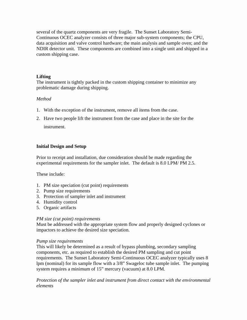
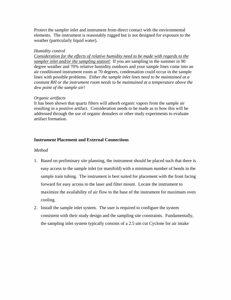
the sampling inlet system typically consists of a 2.5 um cut Cyclone for air intake
and particle size speciation, linked to an organic denuder (note directional flow of
air),
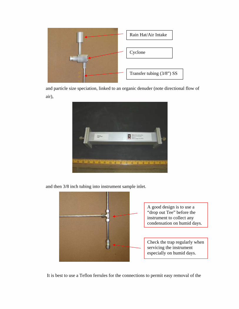
and then 3/8 inch tubing into instrument sample inlet.
It is best to use a Teflon ferrules for the connections to permit easy removal of the
Rain Hat/Air Intake
Cyclone
Transfer tubing (3/8”) SS
A good design is to use a “drop out Tee” before the instrument to collect any condensation on humid days.
Check the trap regularly when servicing the instrument especially on humid days.
sample lines at a later date. Note: Either Copper or S.S tubing can be used. It must
be extremely clean from the standpoint of organics such as manufacturing oils. S.S
tubing is preferred. If there is any doubt as to cleanliness, the tubing can be
cleaned with reagent grade methylene chloride, acetone or methanol and then
dried. Alternately, a propane torch can used to heat the length of tubing while
blowing N2 through the system to remove any volatile organics.
3. Connect the vacuum pump line to the back of the instrument marked “vacuum
pump”. The vacuum pump should have sufficient capacity to pull at least 16 inches
Hg vacuum at 16 lpm. Two different options are available for this configuration:
a. If using a “house vacuum” type system where the pump is on constantly, the
vacuum line should be plumbed into the solenoid valve (provided) on the
“VAC” port. The other side of the solenoid valve should be connected to the
inlet of the ballast tank. The solenoid valve should then be plugged into the
solid state relay control box.
b. If the pump is to be turned on concurrent with the start of sampling, connect
the vacuum pump directly to the ballast tank inlet and plug the pump AC
power to the solid state relay control box. The pump can be run on an
intermittent or continuous basis depending on sampling and noise
requirements.
c. Plug the solid state relay control box to a 120 VAC outlet of sufficient
capacity to support the pump. Large pumps can draw a significant current
load. Plug the digital control cable into the instrument on the “Pump SSR”
control socket.
4. Place the external temperature thermocouple just inside the cyclone rain hat at a point
where the tip is near the sample inlet but out of direct sunlight. Plug the sensor to the
“Ambient Temp” socket.
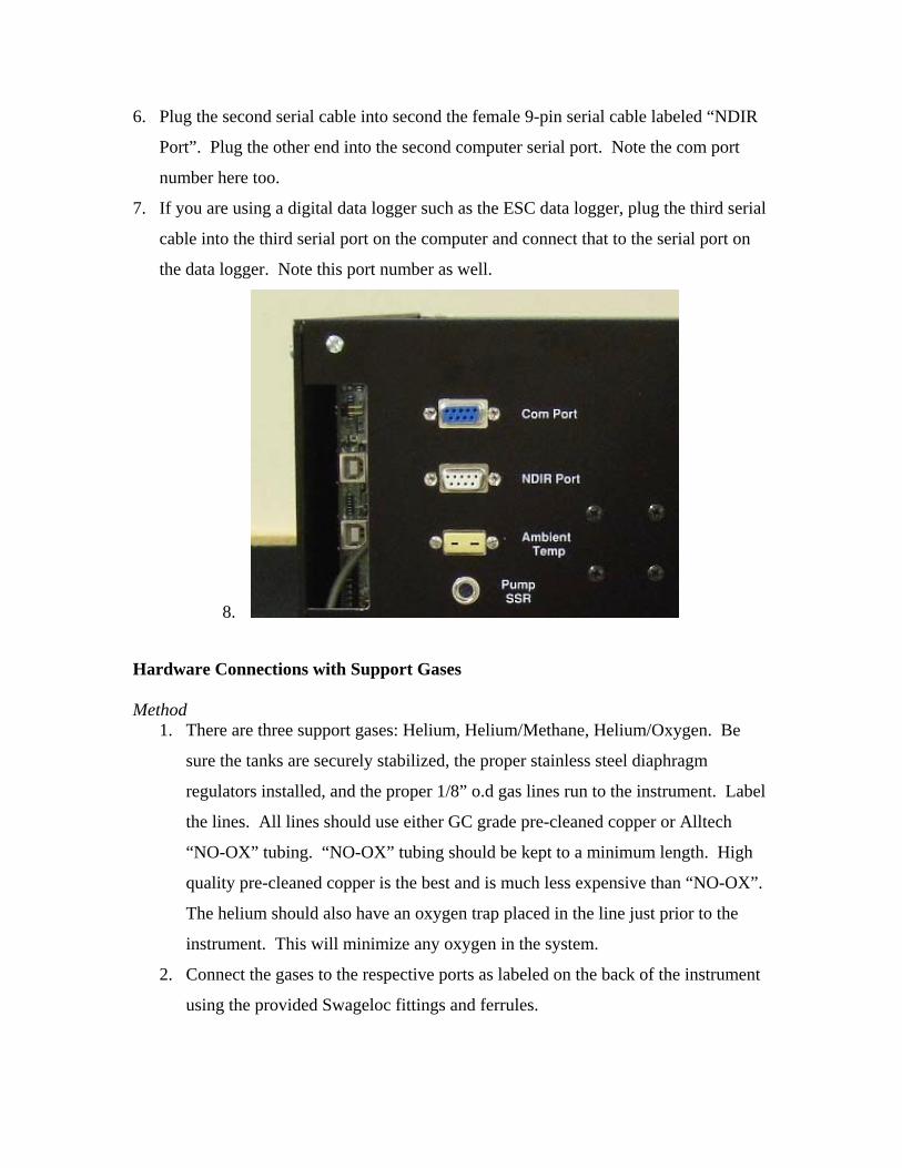
5. Plug the first serial cable into the instrument main board in the top 9-pin female serial
port connector (labeled “Com Port”). Plug the other end into the computer serial port.
If the computer has a hardware serial port, use that for the main communication port.
Note the port number.
6. Plug the second serial cable into second the female 9-pin serial cable labeled “NDIR
Port”. Plug the other end into the second computer serial port. Note the com port
number here too.
7. If you are using a digital data logger such as the ESC data logger, plug the third serial
cable into the third serial port on the computer and connect that to the serial port on
the data logger. Note this port number as well.
8.
Hardware Connections with Support Gases Method
1. There are three support gases: Helium, Helium/Methane, Helium/Oxygen. Be
sure the tanks are securely stabilized, the proper stainless steel diaphragm
regulators installed, and the proper 1/8” o.d gas lines run to the instrument. Label
the lines. All lines should use either GC grade pre-cleaned copper or Alltech
“NO-OX” tubing. “NO-OX” tubing should be kept to a minimum length. High
quality pre-cleaned copper is the best and is much less expensive than “NO-OX”.
The helium should also have an oxygen trap placed in the line just prior to the
instrument. This will minimize any oxygen in the system.
2. Connect the gases to the respective ports as labeled on the back of the instrument
using the provided Swageloc fittings and ferrules.
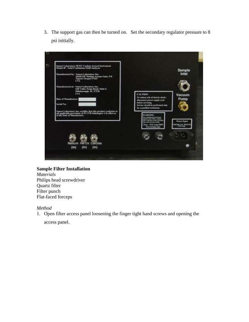
3. The support gas can then be turned on. Set the secondary regulator pressure to 8
psi initially.
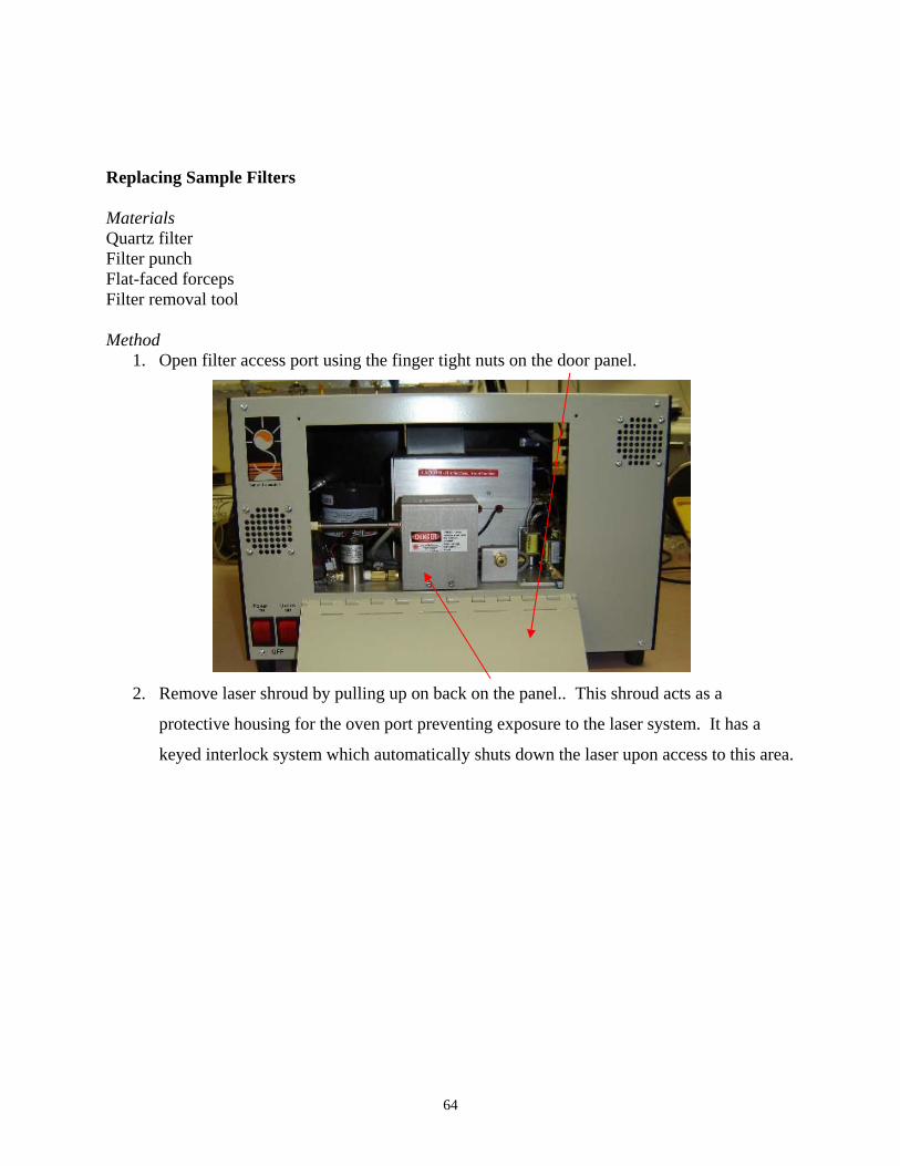
Sample Filter Installation Materials Philips head screwdriver Quartz filter Filter punch Flat-faced forceps Method 1. Open filter access panel loosening the finger tight hand screws and opening the
access panel.
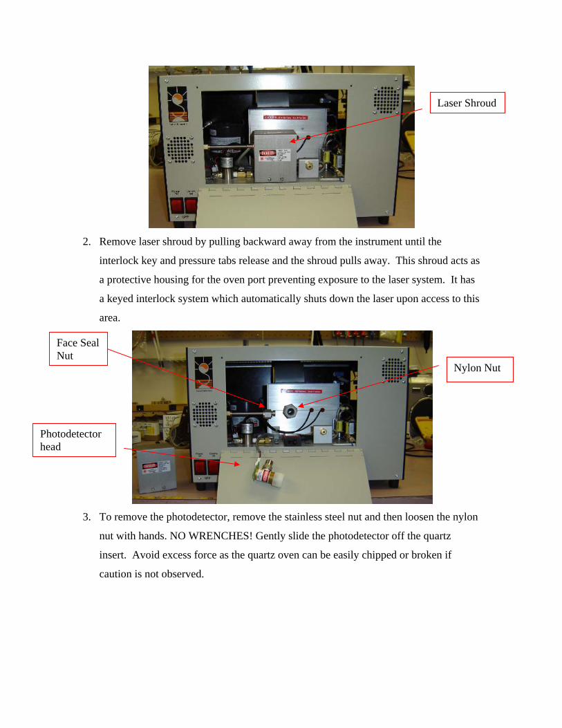
2. Remove laser shroud by pulling backward away from the instrument until the
interlock key and pressure tabs release and the shroud pulls away. This shroud acts as
a protective housing for the oven port preventing exposure to the laser system. It has
a keyed interlock system which automatically shuts down the laser upon access to this
area.
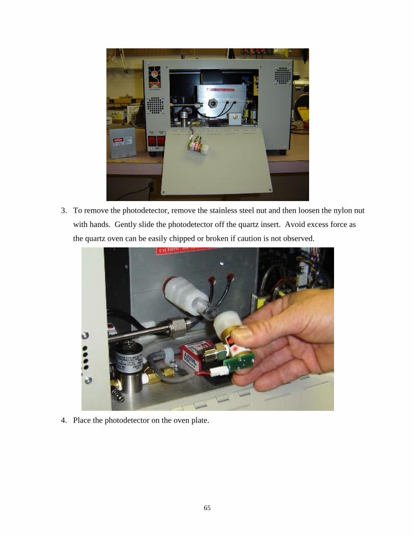
3. To remove the photodetector, remove the stainless steel nut and then loosen the nylon
nut with hands. NO WRENCHES! Gently slide the photodetector off the quartz
insert. Avoid excess force as the quartz oven can be easily chipped or broken if
caution is not observed.
Laser Shroud
Nylon Nut
Face Seal Nut
Photodetector head
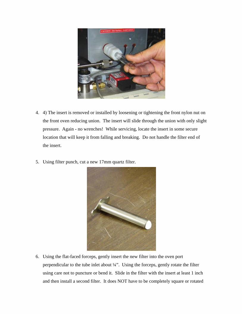
4. 4) The insert is removed or installed by loosening or tightening the front nylon nut on
the front oven reducing union. The insert will slide through the union with only slight
pressure. Again - no wrenches! While servicing, locate the insert in some secure
location that will keep it from falling and breaking. Do not handle the filter end of
the insert.
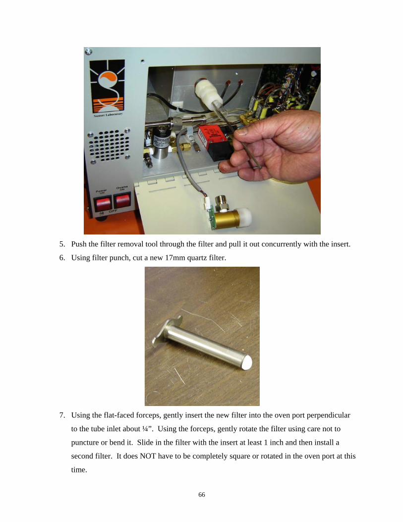
5. Using filter punch, cut a new 17mm quartz filter.
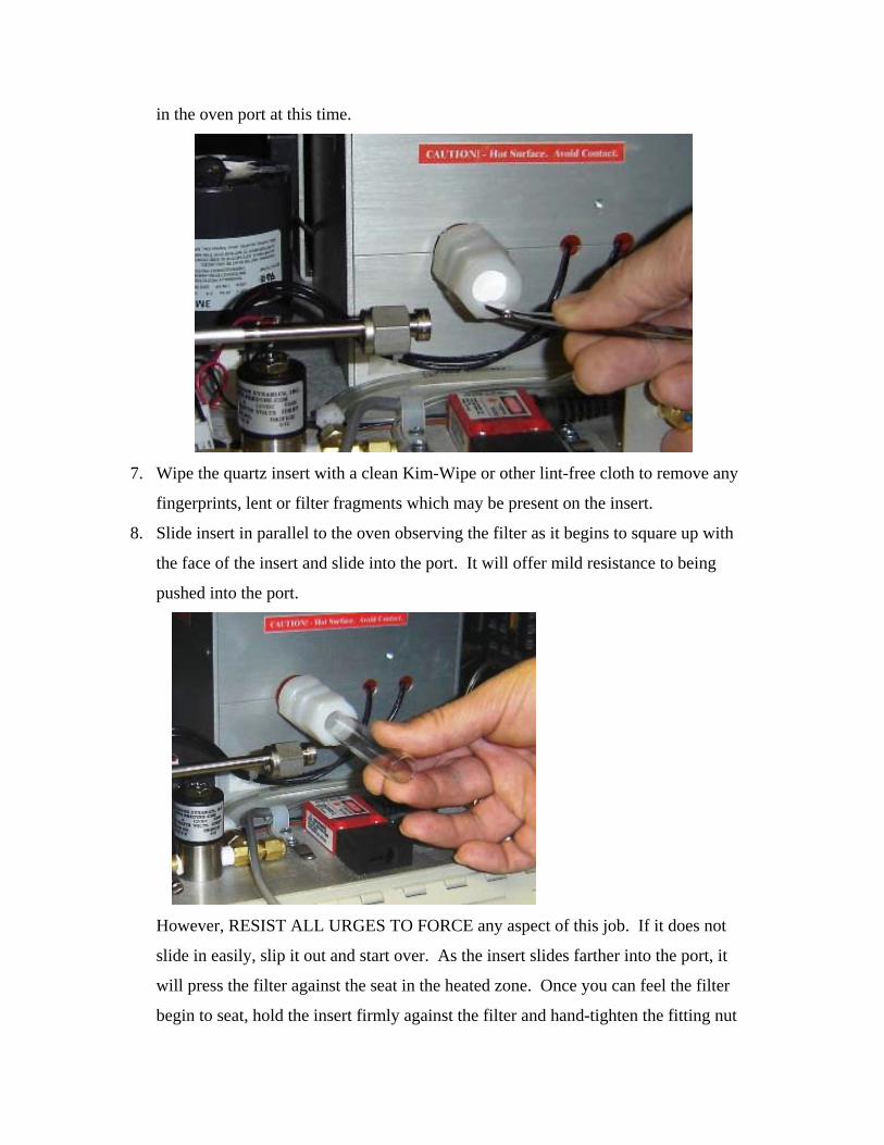
6. Using the flat-faced forceps, gently insert the new filter into the oven port
perpendicular to the tube inlet about ¼”. Using the forceps, gently rotate the filter
using care not to puncture or bend it. Slide in the filter with the insert at least 1 inch
and then install a second filter. It does NOT have to be completely square or rotated
in the oven port at this time.
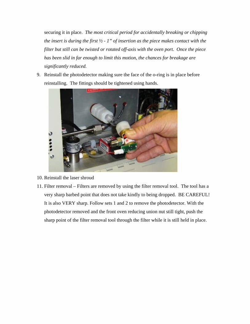
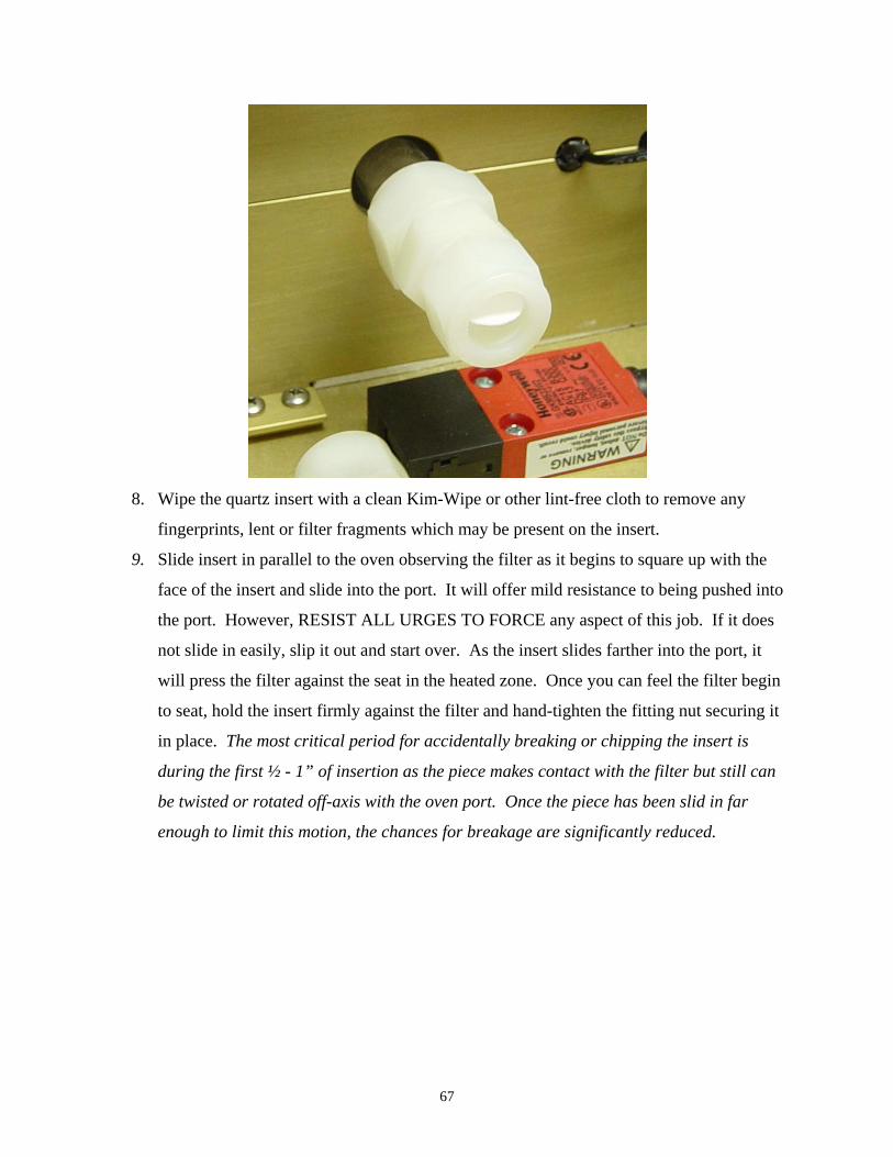
7. Wipe the quartz insert with a clean Kim-Wipe or other lint-free cloth to remove any
fingerprints, lent or filter fragments which may be present on the insert.
8. Slide insert in parallel to the oven observing the filter as it begins to square up with
the face of the insert and slide into the port. It will offer mild resistance to being
pushed into the port.
However, RESIST ALL URGES TO FORCE any aspect of this job. If it does not
slide in easily, slip it out and start over. As the insert slides farther into the port, it
will press the filter against the seat in the heated zone. Once you can feel the filter
begin to seat, hold the insert firmly against the filter and hand-tighten the fitting nut
securing it in place. The most critical period for accidentally breaking or chipping
the insert is during the first ½ - 1” of insertion as the piece makes contact with the
filter but still can be twisted or rotated off-axis with the oven port. Once the piece
has been slid in far enough to limit this motion, the chances for breakage are
significantly reduced.
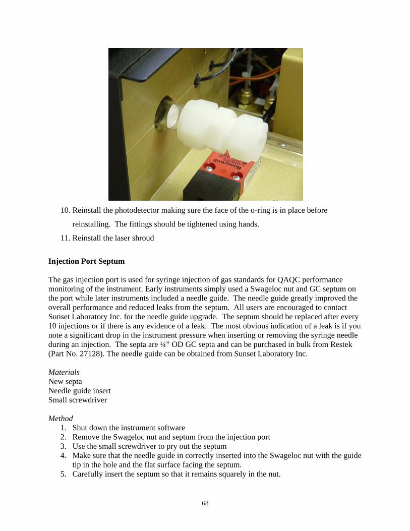
9. Reinstall the photodetector making sure the face of the o-ring is in place before
reinstalling. The fittings should be tightened using hands.
10. Reinstall the laser shroud
11. Filter removal – Filters are removed by using the filter removal tool. The tool has a
very sharp barbed point that does not take kindly to being dropped. BE CAREFUL!
It is also VERY sharp. Follow sets 1 and 2 to remove the photodetector. With the
photodetector removed and the front oven reducing union nut still tight, push the
sharp point of the filter removal tool through the filter while it is still held in place.
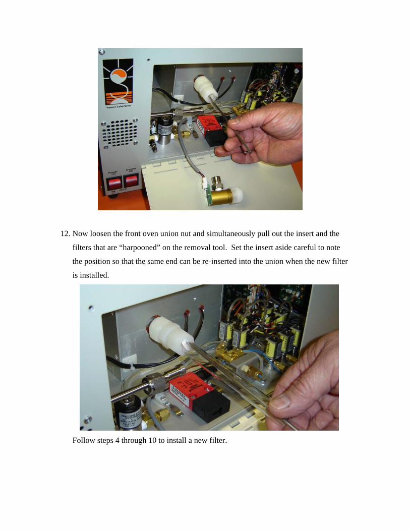
12. Now loosen the front oven union nut and simultaneously pull out the insert and the
filters that are “harpooned” on the removal tool. Set the insert aside careful to note
the position so that the same end can be re-inserted into the union when the new filter
is installed.
Follow steps 4 through 10 to install a new filter.
Software Installation The RT carbon analyzer uses two software programs, one to control the instrument and one to calculate (reprocess) the data. The optional computer from Sunset Laboratory will come with the software installed. Existing computers will need to have the software programs as provided on the accompanying CD installed. A PC-type computer is required for operation of the instrument and must have Microsoft Windows XP Professional; Service Pack 2 installed as the operating system. (Win 2K service pack 4 is still supported but not preferred. Windows VISTA is not supported). Instruments delivered within the United States will be shipped with a new computer with the current software pre-installed and tested. Warranty on Sunset Laboratory Inc. provided computers shall be for 90 days only. Any repairs or damage after the warranty period shall be the responsibility of the purchaser. International purchases may include a computer as an option where allowed by United States export laws. At a minimum, the computer, whether provided by Sunset Laboratory Inc. or the client, shall include:
1. Windows XP Professional; Service Pack 2. (We currently have no experience with the new Windows Vista operating system. For the time being, we are only supporting XP Professional until the Vista system can be thoroughly investigated and any necessary software changes made to adapt to the new system.)
2. 2 GHz processor or better 3. 512 Mb ram 4. Read/Write CD/Rom 5. 2 serial ports. Serial ports may be directly from the main computer CPU board or
USB2.0-to-Serial converter cables. On client provided computers, it is the obligation of the client to configure the serial ports and assure that there are no conflicts between ports or interrupts. We will help where we can but it is your obligation.
6. Small footprint computer case or laptop Method
1. You must run first the “setup.exe” file provided with the disk (or file upload) in the
Setup subfolder under the main Install folder.
2. After you run the setup file, you must then change the format of at least one file and
move several others.
3. First, note the location (default) of the new software:
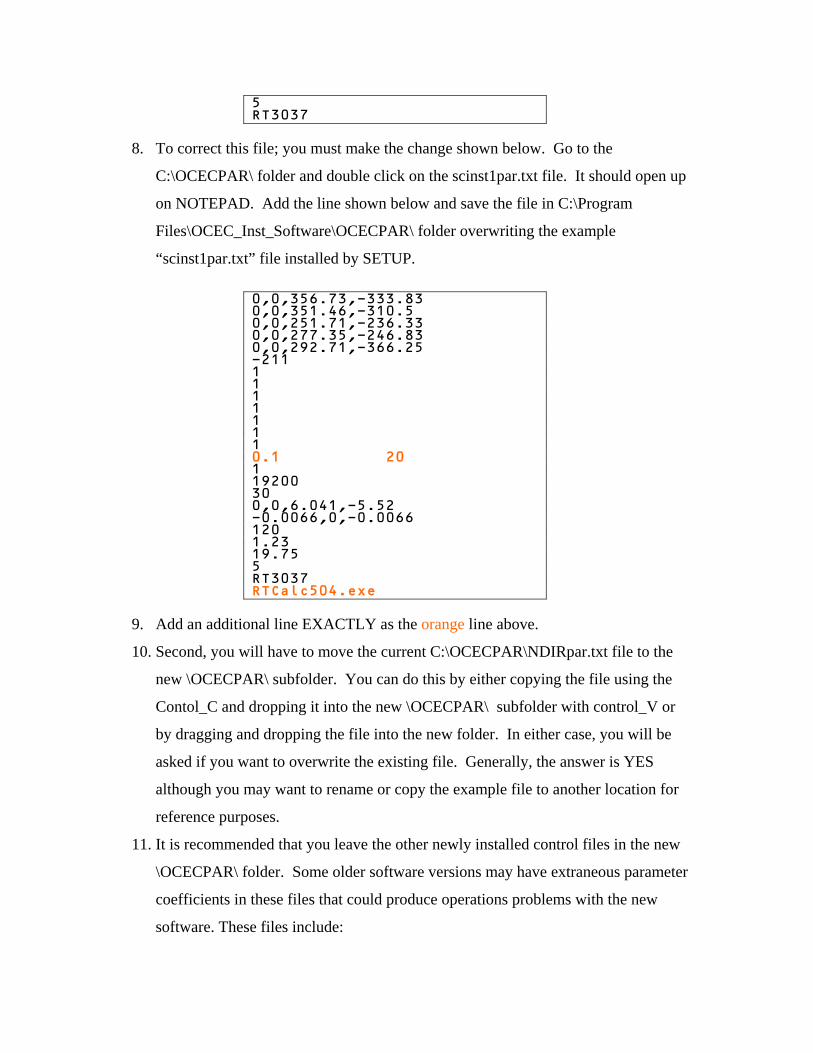
9. Add an additional line EXACTLY as the orange line above.
10. Second, you will have to move the current C:\OCECPAR\NDIRpar.txt file to the
new \OCECPAR\ subfolder. You can do this by either copying the file using the
Contol_C and dropping it into the new \OCECPAR\ subfolder with control_V or
by dragging and dropping the file into the new folder. In either case, you will be
asked if you want to overwrite the existing file. Generally, the answer is YES
although you may want to rename or copy the example file to another location for
reference purposes.
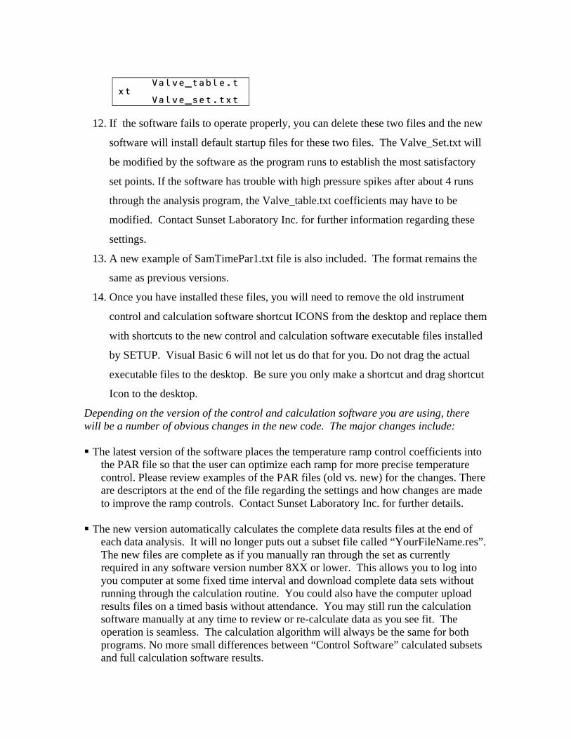
11. It is recommended that you leave the other newly installed control files in the new
\OCECPAR\ folder. Some older software versions may have extraneous parameter
coefficients in these files that could produce operations problems with the new
software. These files include:
Valve_table.txt Valve_set.txt
12. If the software fails to operate properly, you can delete these two files and the new
software will install default startup files for these two files. The Valve_Set.txt will
be modified by the software as the program runs to establish the most satisfactory
set points. If the software has trouble with high pressure spikes after about 4 runs
through the analysis program, the Valve_table.txt coefficients may have to be
modified. Contact Sunset Laboratory Inc. for further information regarding these
settings.
13. A new example of SamTimePar1.txt file is also included. The format remains the
same as previous versions.
14. Once you have installed these files, you will need to remove the old instrument
control and calculation software shortcut ICONS from the desktop and replace them
with shortcuts to the new control and calculation software executable files installed
by SETUP. Visual Basic 6 will not let us do that for you. Do not drag the actual
executable files to the desktop. Be sure you only make a shortcut and drag shortcut
Icon to the desktop.
Depending on the version of the control and calculation software you are using, there will be a number of obvious changes in the new code. The major changes include: The latest version of the software places the temperature ramp control coefficients into
the PAR file so that the user can optimize each ramp for more precise temperature control. Please review examples of the PAR files (old vs. new) for the changes. There are descriptors at the end of the file regarding the settings and how changes are made to improve the ramp controls. Contact Sunset Laboratory Inc. for further details.
The new version automatically calculates the complete data results files at the end of
each data analysis. It will no longer puts out a subset file called “YourFileName.res”. The new files are complete as if you manually ran through the set as currently required in any software version number 8XX or lower. This allows you to log into you computer at some fixed time interval and download complete data sets without running through the calculation routine. You could also have the computer upload results files on a timed basis without attendance. You may still run the calculation software manually at any time to review or re-calculate data as you see fit. The operation is seamless. The calculation algorithm will always be the same for both programs. No more small differences between “Control Software” calculated subsets and full calculation software results.
The new software has better control of the flows on the of the carrier gases. Adjust
your carrier gas inlet pressures to between 15 and 30 PSI for R4 instruments (6 to 8 for R3 instruments). The control software will then optimize the starting points for each mode over the course of several analyses and refine those as conditions change.
After the system has run for several cycles, you can “AUTOZERO” the gas flows. This
is performed by having the system in “IDLE”. Check the Valve_Values_Table on the lower screen. When the window pops up, hit the “AUTOZERO Gases” button and wait for the instrument to complete the cycle. It will then save the new zero intercepts in the scinst1par.txt file for current and future reference.
There is an “Autostart” function that pops up each time the software is started. If left
unattended, it will automatically start the instrument up in using the Sample File named SamTimePar1.txt located in the \OCECPAR\ subfolder. This is useful for recovering from a power failure. If the software is installed on a newer desktop, the user can go into the computer setup files available at the startup of the computer and set the power recovery mode to restart the computer after the loss of power. If a shortcut to the RT OCEC software has been placed in the “All Users” startup menu, then the system will recover and Autostart from a hard power failure unattended. Laptops should use one of the newer UPS systems which will keep the laptop operational for up to 2 days after a power failure. The software will recover and restart the instrument in either case once power is restored.
The new software has a number of new Error Message boxes that pop up in the event of
a number of problems that may occur. These include the loss of support gases and the failure to heat as a result of a burned out heating coil.
Two different options for digital output to a data logger are available. The default is a
formatted but not fixed length format while a fixed length format can be selected by checking a box in the lower screen. Contact Sunset Laboratory for more information on this option.
Several bugs and errors that were a nagging problem with the older software have been
corrected. These include the occasional failure to write results files to the disk that were the result of a “Divide by Zero” error. This apparently was embedded in the old calculation routine in the control software. This has been removed.
The use of “0” time collections for QAQC purposes no longer results in the loss of the
“Start Analysis” button that sometimes occurred in the older software requiring a restart to clear the flag.
The new software versions will collect samples up to 24 hours without hanging up.
Serial port configuration - NDIRpar.txt and Scinst1par.txt files
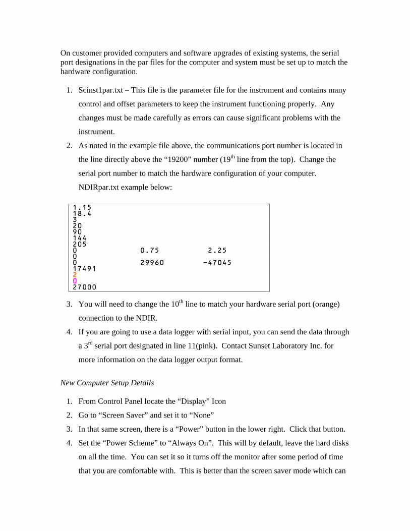
On customer provided computers and software upgrades of existing systems, the serial port designations in the par files for the computer and system must be set up to match the hardware configuration.
1. Scinst1par.txt – This file is the parameter file for the instrument and contains many
control and offset parameters to keep the instrument functioning properly. Any
changes must be made carefully as errors can cause significant problems with the
instrument.
2. As noted in the example file above, the communications port number is located in
the line directly above the “19200” number (19th line from the top). Change the
serial port number to match the hardware configuration of your computer.
3. You will need to change the 10th line to match your hardware serial port (orange)
connection to the NDIR.
4. If you are going to use a data logger with serial input, you can send the data through
a 3rd serial port designated in line 11(pink). Contact Sunset Laboratory Inc. for
more information on the data logger output format.
New Computer Setup Details
1. From Control Panel locate the “Display” Icon
2. Go to “Screen Saver” and set it to “None”
3. In that same screen, there is a “Power” button in the lower right. Click that button.
4. Set the “Power Scheme” to “Always On”. This will by default, leave the hard disks
on all the time. You can set it so it turns off the monitor after some period of time
that you are comfortable with. This is better than the screen saver mode which can
consume a considerable quantity of memory and cause the software to drop
communications.
5. In the “Advanced” tab, it is recommended that you have the computer ask you what
to do when you press the “shut off” button.
6. On laptops, have it “do nothing” when you close the top. It should not ever go into
“sleep” or “hibernate” mode.
7. If you have purchased a small desktop, you can go into the EEPROM setup of you
computer when it starts up by holding the F2 key. In the POWER scheme, you can
have it Resume what ever condition is was in the event of a power outage. For
example, if it was on (and presumably collecting samples) it would re-boot when
power comes back.
8. You should set the computer up so that the default user does not have a password
and does not come up in the “Welcome” screen.
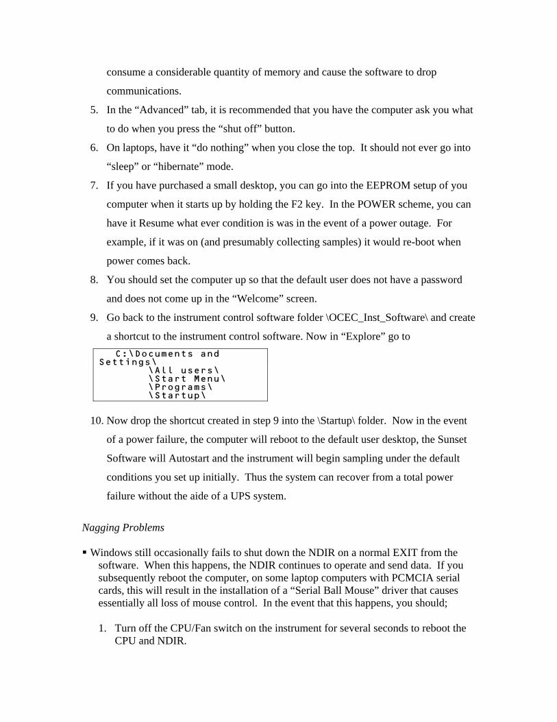
9. Go back to the instrument control software folder \OCEC_Inst_Software\ and create
a shortcut to the instrument control software. Now in “Explore” go to
C:\Documents and Settings\ \All users\ \Start Menu\ \Programs\ \Startup\
10. Now drop the shortcut created in step 9 into the \Startup\ folder. Now in the event
of a power failure, the computer will reboot to the default user desktop, the Sunset
Software will Autostart and the instrument will begin sampling under the default
conditions you set up initially. Thus the system can recover from a total power
failure without the aide of a UPS system.
Nagging Problems Windows still occasionally fails to shut down the NDIR on a normal EXIT from the
software. When this happens, the NDIR continues to operate and send data. If you subsequently reboot the computer, on some laptop computers with PCMCIA serial cards, this will result in the installation of a “Serial Ball Mouse” driver that causes essentially all loss of mouse control. In the event that this happens, you should;
1. Turn off the CPU/Fan switch on the instrument for several seconds to reboot the
CPU and NDIR.
2. Shut down the computer. While it is down, pull out the PCMCIA card. Restart the computer. After it completely recovers, then re-insert the PCMCIA card. This should clear the problem driver condition.
3. In the future, if you are going to shut down and reboot (as we suggest every time you service the instrument) then you should also turn off the CPU/fan switch on the instrument to clear it as well. This will prevent the previous problem.
Occasionally, there are serial communication losses. This is not common but can
usually be corrected by setting the serial buffers to a smaller value so that Windows services these more frequently. Ask Sunset Laboratory about how to set these up for your system.
Oven Installation The main quartz oven has two heated zones: the front oven and the back oven. New instruments will have the oven and heating coils installed, conditioned and ready to operate. The front oven is used to collect and analyze the samples. It is only heated during the analysis phase while remaining at or near ambient temperature during the sampling phase. The back oven contains the MnO2 oxidizer and is heated to 850oC during the analysis phase. In order to insure a controlled sample temperature, the back oven is maintained at 500oC during sampling. The two zones will be delivered pre-configured to perform at the prescribed temperatures and the oven installed. For the procedure for oven installation, see the servicing chapter on page ____.
Laser Installation The laser is mounted within the optical system and no mounting or adjustment is necessary. For the procedure for the laser setup, see the servicing chapter on page ____. NDIR Signal The NDIR serial port is connected to the 9-pin DIN connector located on the back/center of the instrument. This cable is connected to the other serial port on the computer. 1. Go to the “C:\ocecpar\ndirpar.txt” file and type in the correct serial port number (2 –
6). (See section “Files used by the Sunset Laboratory Inc. RT-OCEC analyzer”).
2. When the instrument starts, the “CO2” signal reported on the screen will begin
reporting a CO2 level after about a minute of software initialization.
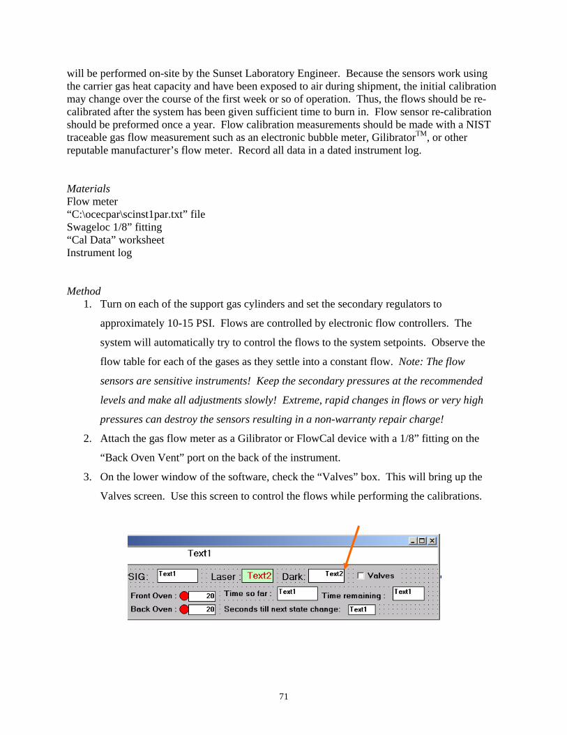
Flow Sensor Calibration The instrument will come with an initial flow calibration from the factory. The flow calibration parameters are contained in the “C:\ocecpar\scinst1par.txt” file. Flow sensor calibration is a multi-step process which must be performed in the correct order. Initial offsets and a calibration check will be performed on-site by the Sunset Laboratory Engineer. Because the sensors work using the carrier gas heat capacity and have been exposed to air during shipment, the initial calibration may change over the course of the first week or so of operation. Thus, the flows should be re-calibrated after the system has been given sufficient time to burn in. Observe the Sunset Laboratory Engineer carefully during this phase of the installation and follow the procedure carefully. If performed properly and the data logged correctly into the instrument parameter file, the observed flow reading on the flow table should be correct (± 5 %) for an extended period. Re-calibration once a year is recommended. The slope values for the sensors tend to remain fairly constant over time but the Zeros do drift. It is recommended that you AutoZero the sensors each week as a routine procedure while servicing the instrument. Initialization 1. Switch on the CPU/Fan switch to the Main Oven Box only!! Do not turn on the
heated zone power yet!
2. Click on the Semi-Continuous OCEC Startup Icon. The system should begin
operation by reporting temperatures and showing flow sensor flow rates.
3. If the system does not start, shut down the software from the PC and restart.
4. If it does not start this time, go into the “C:\ocecpar\scinst1par.txt” file and be sure
the serial port setting is correct (1 – 6) for the instrument and try again. (See section
“Files used by the Sunset Laboratory Inc. RT-OCEC analyzer”). The instrument
software should start and begin controlling the instrument. If you have problems,
contact your Sunset Laboratory Representative.
Final Installation Steps 1. Restart the software to initialize the new coefficients. The software will control the
flows for each of the sample and analysis modes. The temperature for the “Back
Oven” should begin to climb on the software monitor screen. After a short period of
time, this will stabilize at their preset default settings: 500°C.
2. After this has been operational for at least 15 minutes, go to the menu and run the
“Clean Oven” step. This will heat front oven to clean it out and burn off any residual
binder from the heating coil sheathing, clean off the new filters and remove any
residual organic material from the front oven. The instrument should now be fully
configured and ready to perform the carbon calibrations and begin running samples.
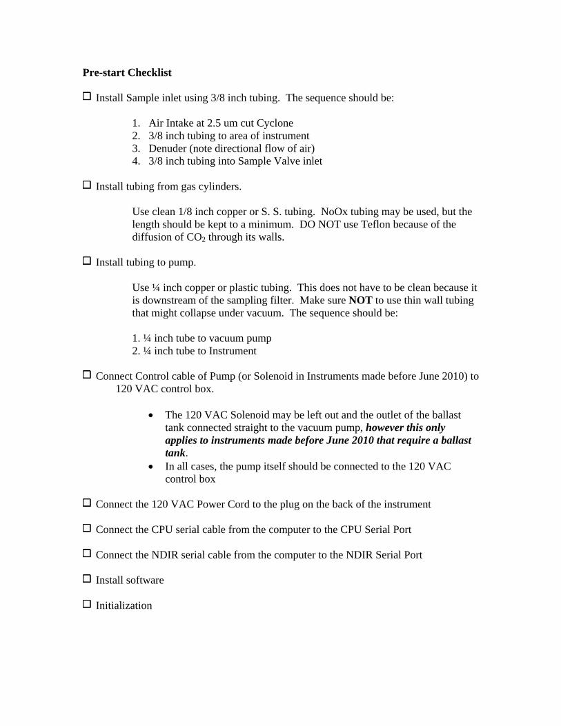
Pre-start Checklist
Install Sample inlet using 3/8 inch tubing. The sequence should be: 1. Air Intake at 2.5 um cut Cyclone 2. 3/8 inch tubing to area of instrument 3. Denuder (note directional flow of air) 4. 3/8 inch tubing into Sample Valve inlet
Install tubing from gas cylinders.
Use clean 1/8 inch copper or S. S. tubing. NoOx tubing may be used, but the length should be kept to a minimum. DO NOT use Teflon because of the diffusion of CO2 through its walls.
Install tubing to pump.
Use ¼ inch copper or plastic tubing. This does not have to be clean because it is downstream of the sampling filter. Make sure NOT to use thin wall tubing that might collapse under vacuum. The sequence should be:
1. ¼ inch tube to vacuum pump 2. ¼ inch tube to Instrument
Connect Control cable of Pump (or Solenoid in Instruments made before June 2010) to
120 VAC control box.
The 120 VAC Solenoid may be left out and the outlet of the ballast tank connected straight to the vacuum pump, however this only applies to instruments made before June 2010 that require a ballast tank.
In all cases, the pump itself should be connected to the 120 VAC control box
Connect the 120 VAC Power Cord to the plug on the back of the instrument
Connect the CPU serial cable from the computer to the CPU Serial Port
Connect the NDIR serial cable from the computer to the NDIR Serial Port
Install software
Initialization
Operation The purpose of this section is to provide information on the use of the instrument. Software overview A PC-type computer is required for operation of the instrument and must have Microsoft Windows XP Professional (Service Pack 2 or higher) installed as the operating system. Windows VISTA(updated with all Service Pack 2) and Windows 7 are also compatible and may be used. The software for instrument operation and results calculations are designed to run on the included Computerized Display/Data Acquisition System. This software is included with the Base Instrument. The PC based software is currently written in Microsoft Visual Basic 6.0. Software is provided either with a computer supplied by Sunset Laboratory or on an Installation disk. (See software installation section XYZ2)
1. Instrument Operation Application - controls the instrument operation and data collection during sample analysis; saves the raw data for calculations later.
2. Calculation Application - uses the raw data produced from the instrument and
calculates organic and elemental carbon, creates a spreadsheet-usable reduced data file of the results and optional prints the individual analysis report.
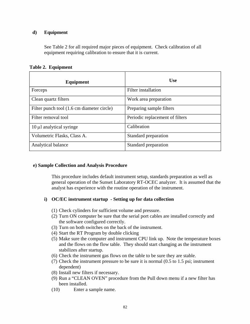
Controls on the instrument Essentially all of the control components of the instrument are controlled by the PC. The user can set up most all of the variable features from within the software environment. See section XX below for a complete discussion of the software. Samples The analyzer is deployed to the field site. It collects airborne particulate samples on an internally mounted filter and analyzes the sample on a semi-continuous basis. There is no option for replicates without a second sampler. Sample data are stored in raw data files. Additionally, a short result file is printed to a file at the end of each analysis. An optional output can also be transmitted to a data logger equipped with a serial input. The data should be considered irreplaceable and should be backed up on a frequent basis to some sort of permanent media such a CD or tape. Materials and equipment
See the example Standard Operating Procedure In Section XXX for a detailed discussion of the required materials and equipment for routine sample collection and instrument calibration and maintenance. Operating parameters
Quartz Punch Size: 16.5 mm diameter punched using the provided filter punch. Deposit size related to insert inlet size
Standard Analysis time: ~ 8.5 minutes (not including 2 minutes of
purging time). Other methods are possible by change the appropriate parameters
Sampling Time: pull-down list options ; or file controlled
Check up the box for “cycle” to continuously measure OC/EC. Then the
instrument starts to run on the following minute.
Check “start analysis” button for 1 cycle measurement.
Clear the check mark for “cycle” to make the current measurement the last measurement.
Output Data o During sampling, data is averaged every 1 minute. o During analysis, data is averaged every 1 second. o Data is saved and a complete set of calculations are performed at the
end of the analysis. o Preliminary EC/TC measurements are calculated and plotted at the end
of each analysis.
Output file can be copied and calculated during sampling, but not during analysis of the current sample. This will result in a “file conflict” error and could terminate the run.
Windows XP Professional is recommended as computer operating
program. Window 98 could cause some problems in the communication between computer and the analyzer. Windows Vista is not currently supported
Output Data file name is not updated while collecting the sample or
analyzing. The measurement data are stored in the file at the end of each analysis. Disruptions in the operation result in the data loss only for the current sample.
Startup and Running a Sample (the Short List)
Before proceeding, assure that the gas lines are properly connected to the back of the instrument and that the gas cylinder valves are all open and the secondary regulator pressures are set from 8 to 10 PSI on Model 3 instruments and 15 – 20 PSI on Model 4 instruments. Also, if there are ON/OFF valves inline for the gases, make sure they are open.
1. Check cylinders for sufficient volume and pressure. 2. Be sure that the serial port cables are installed correctly and the software
configured correctly. 3. Turn on the Computer. 4. Turn ON both switches of the Semi-Continuous OCEC Instrument (the back left
hand side for Model 3 and lower right front for Model 4). Then start the RTOCEC application program on the PC by clicking on the ICON located on the Desktop.
5. Make sure the computer and instrument CPU link up. Note the temperature boxes and the flows on the flow table. They should start changing as the instrument stabilizes after startup.
6. Check the pressure. In the Off-line Mode it should be in the range of 0.1 to 0.5 psi depending upon flow rates and temperature of the Back Oven. While analyzing On-Line, it should increase to as much as 3.0 psi.. This Oven pressure will change, depending upon flow rates and resistances of the MnO2 Oxidizer Bed.
7. Check the instrument gas flows on the table to be sure they are stable. 8. Install new filters if necessary. 9. Clean Oven by selecting CLEAN OVEN from the OPTIONS Menu. 10. Enter a sample name in the SAMPLE ID #. 11. Select the proper PARAMETER FILE to be used for analyzing the samples. By
default it is “rtquartz.par”. 12. If you desire the raw data to go into an automatically generated file each day, the
default ending of “\” is already selected. To have the data go into a file of another name, type the name of the file in the OUTPUT RAW DATA FILE box after the “\” already there. Be sure and end the filename with the extension “txt”(example: yourfilename.txt)
13. Determine how the instrument will be cycled; either by sampling for a fixed time followed by the analysis; or by starting sampling times and pre-determined times and lengths from an external file.
14. Make sure the Cycle Box is checked for continuous operation. 15. Click on “Start”.
Shutdown
1. If you are intending to return to the Analyzer later in the day or over the next several days click on the upper left “Run” menu and “Exit All Off”
2. Switch off the “Power” switches. 3. Close all of the gases at the regulators on the cylinders. 4. Go have a Beer.
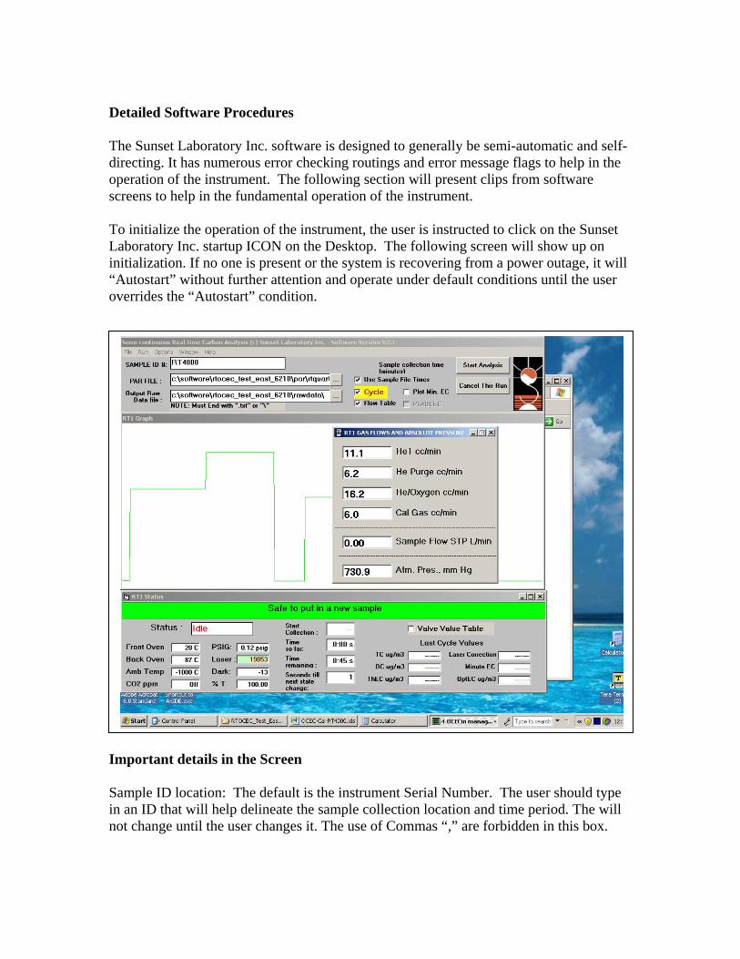
Detailed Software Procedures The Sunset Laboratory Inc. software is designed to generally be semi-automatic and self-directing. It has numerous error checking routings and error message flags to help in the operation of the instrument. The following section will present clips from software screens to help in the fundamental operation of the instrument. To initialize the operation of the instrument, the user is instructed to click on the Sunset Laboratory Inc. startup ICON on the Desktop. The following screen will show up on initialization. If no one is present or the system is recovering from a power outage, it will “Autostart” without further attention and operate under default conditions until the user overrides the “Autostart” condition.
Important details in the Screen Sample ID location: The default is the instrument Serial Number. The user should type in an ID that will help delineate the sample collection location and time period. The will not change until the user changes it. The use of Commas “,” are forbidden in this box.
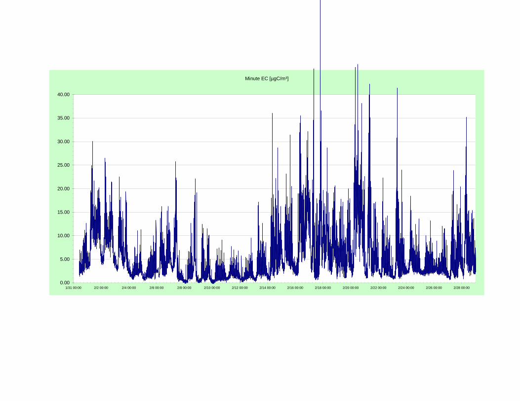
PAR File: This is the sample analysis protocol. The default is RT-Quartz.par and is a short version of the NIOSH 5040. Output Raw Data File: This is the folder location of the raw and post-run calculated data. If the user leaves the file format (default) as shown – c:\....\rawdata\ then the raw data and calculated data will be automatically named in the format “SLI_date_code.TXT”and will be changed every day at midnight to reflect the new data. If the user opts to put in their own name, then it will remain until changed by the user. All files are appended and never overwritten to avoid loss of data. “Use Sample File Times” Checkbox: The default is to use the a file called “SamTimePar1.txt” to define the sample start times. When un-checked, a run time menu will appear that allows the user to choose a fixed collection time. The instrument will collect and analyze samples as fast as possible within this time limits “Cycle” checkbox: The default is “Checked” and causes the instrument to collect and analyze samples until told to stop “Flow Table” checkbox: The default is “checked” and causes the Flow rate Table to be drawn on the screen. This can be moved to a position just off of the run-time screen for continuous viewing. “Plot Min. EC” Checkbox: The default is “Un-Checked”. This box will plot the “once per minute” optical EC during the sample collection on the screen. This is only for user observation. No files are created from the use of this box. A “Minute-EC” file is always created with the data calculation so that the user can observe and plot the Optical EC with every data set. “Valve Values Table” Checkbox: The default is “Un-Checked”. This box brings up the voltage control valve controls used in the mass flow control of the carrier gases. This is a very powerful tool that will be discussed more thoroughly below. More instrument parameters and control information is available by expanding the lower RT1 Status screen.
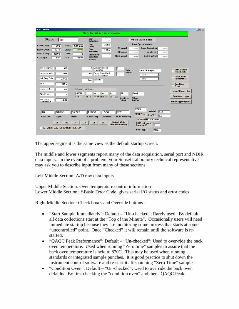
The upper segment is the same view as the default startup screen. The middle and lower segments report many of the data acquisition, serial port and NDIR data inputs. In the event of a problem, your Sunset Laboratory technical representative may ask you to describe input from many of these sections. Left-Middle Section: A/D raw data inputs Upper Middle Section: Oven temperature control information Lower Middle Section: SBasic Error Code, gives serial I/O status and error codes Right Middle Section: Check boxes and Override buttons.
“Start Sample Immediately”: Default – “Un-checked”; Rarely used. By default, all data collections start at the “Top of the Minute”. Occasionally users will need immediate startup because they are monitoring some process that starts at some “uncontrolled” point. Once “Checked” it will remain until the software is re-started.
“QAQC Peak Performance”: Default – “Un-checked”; Used to over-ride the back oven temperature. Used when running “Zero time” samples to assure that the back oven temperature is held to 870C. This may be used when running standards or integrated sample punches. It is good practice to shut down the instrument control software and re-start it after running “Zero Time” samples
“Condition Oven”: Default – “Un-checked”; Used to override the back oven defaults. By first checking the “condition oven” and then “QAQC Peak
Performance” boxes, the user can then highlight the “Desired Back Oven Temperature” value (500 in the screen display) and type in another temperature. This is used to condition a new oven or may be used by the Sunset Lab technician to correct a problem.
Reload Parameter Files Button – If you make changes such a s flow sensor calibration coefficients, these can be reloaded dynamically by “hitting” this button. You should only do this in the “Idle” mode. This is most useful while performing flow calibrations. Do not use this while collecting or analyzing a sample. The very best way to be sure that all of the parameters are reloaded is by shutting down the software and re-starting.
Test Data Logger Button – Sends a test string to the appointed data logger serial port.
Lower Section: NDIR Data and control buttons. These should only be used when directed by your Sunset Laboratory technical representative during trouble shooting.
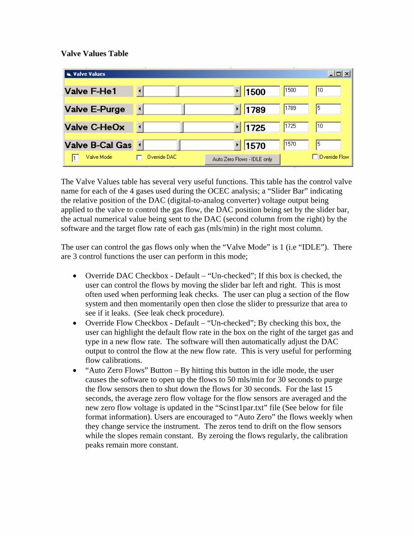
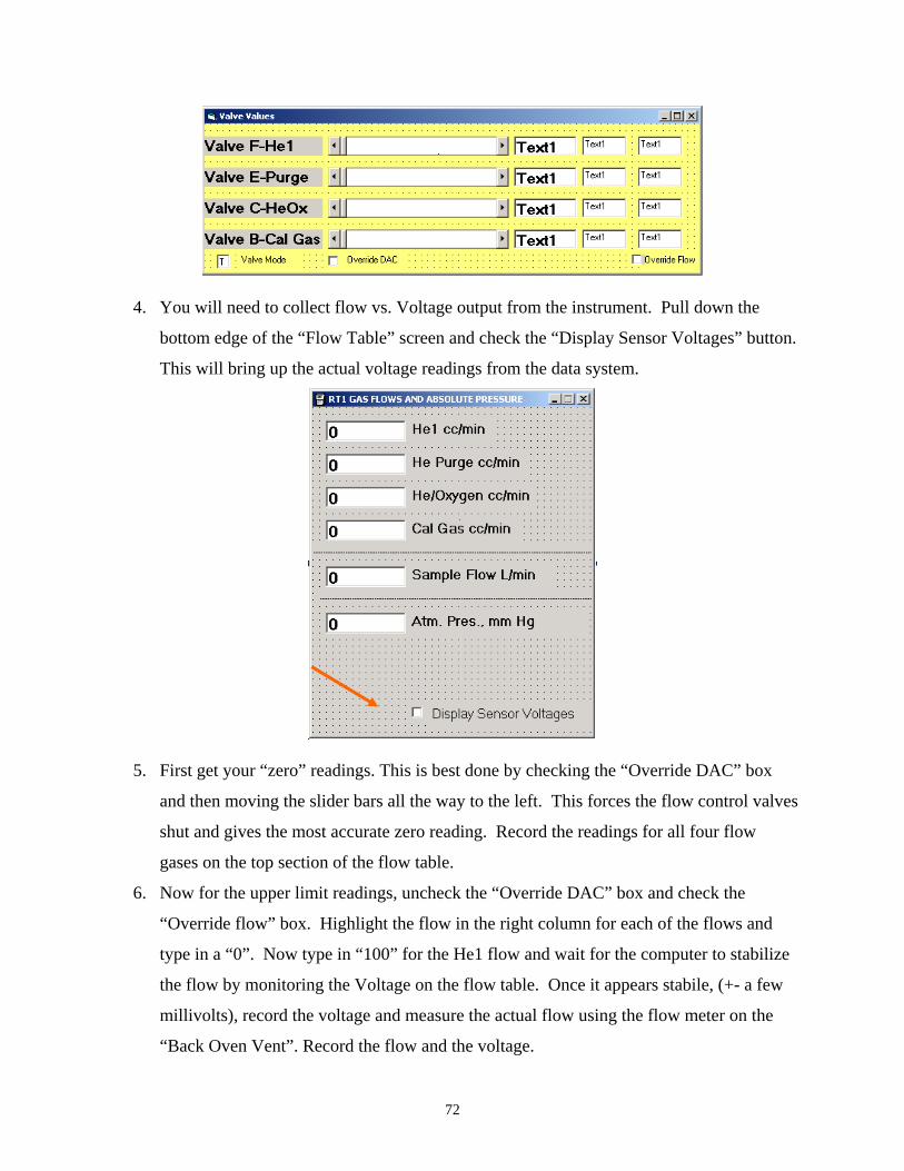
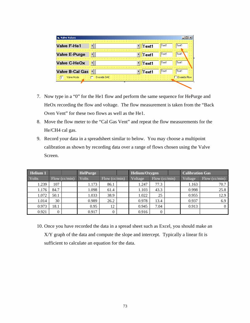
Valve Values Table
The Valve Values table has several very useful functions. This table has the control valve name for each of the 4 gases used during the OCEC analysis; a “Slider Bar” indicating the relative position of the DAC (digital-to-analog converter) voltage output being applied to the valve to control the gas flow, the DAC position being set by the slider bar, the actual numerical value being sent to the DAC (second column from the right) by the software and the target flow rate of each gas (mls/min) in the right most column. The user can control the gas flows only when the “Valve Mode” is 1 (i.e “IDLE”). There are 3 control functions the user can perform in this mode;
Override DAC Checkbox - Default – “Un-checked”; If this box is checked, the user can control the flows by moving the slider bar left and right. This is most often used when performing leak checks. The user can plug a section of the flow system and then momentarily open then close the slider to pressurize that area to see if it leaks. (See leak check procedure).
Override Flow Checkbox - Default – “Un-checked”; By checking this box, the user can highlight the default flow rate in the box on the right of the target gas and type in a new flow rate. The software will then automatically adjust the DAC output to control the flow at the new flow rate. This is very useful for performing flow calibrations.
“Auto Zero Flows” Button – By hitting this button in the idle mode, the user causes the software to open up the flows to 50 mls/min for 30 seconds to purge the flow sensors then to shut down the flows for 30 seconds. For the last 15 seconds, the average zero flow voltage for the flow sensors are averaged and the new zero flow voltage is updated in the “Scinst1par.txt” file (See below for file format information). Users are encouraged to “Auto Zero” the flows weekly when they change service the instrument. The zeros tend to drift on the flow sensors while the slopes remain constant. By zeroing the flows regularly, the calibration peaks remain more constant.
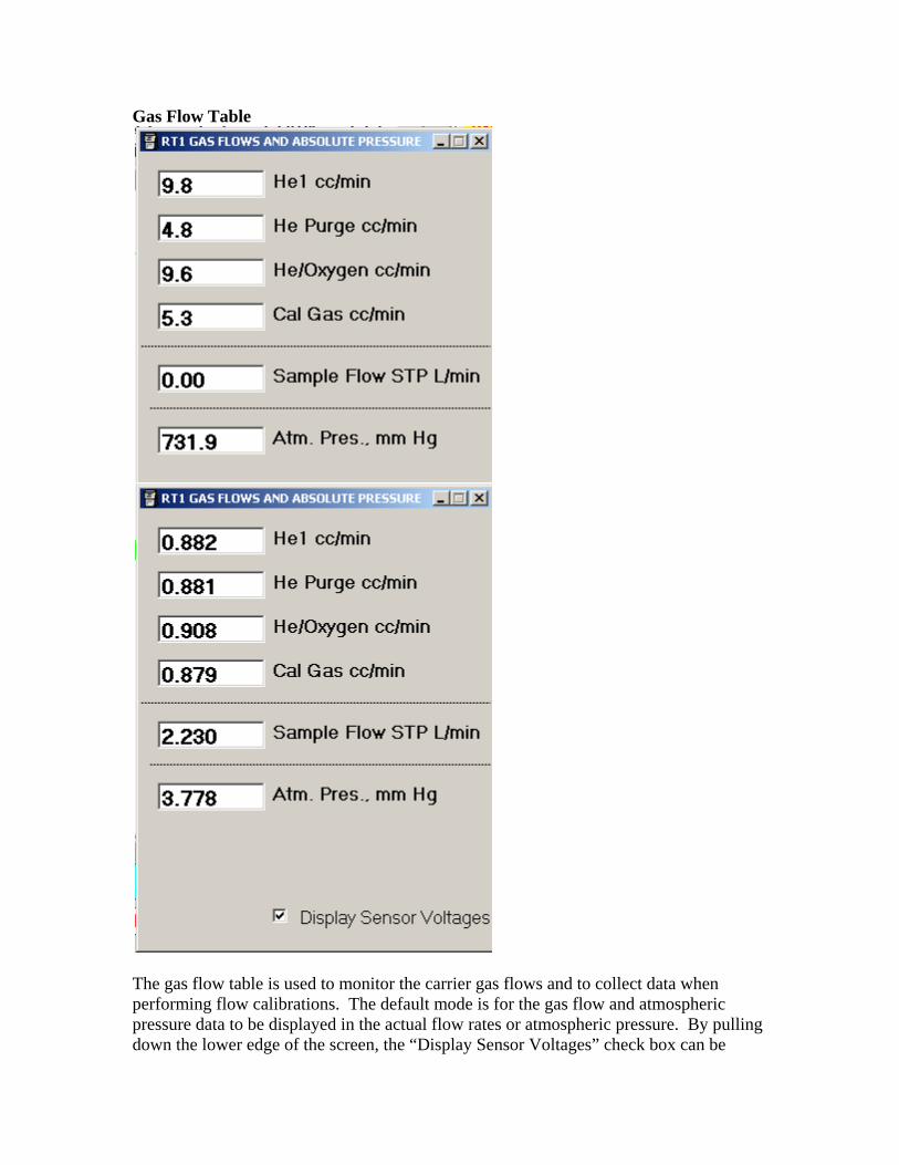
Gas Flow Table
The gas flow table is used to monitor the carrier gas flows and to collect data when performing flow calibrations. The default mode is for the gas flow and atmospheric pressure data to be displayed in the actual flow rates or atmospheric pressure. By pulling down the lower edge of the screen, the “Display Sensor Voltages” check box can be
exposed (Default – “Un-checked”). When checked, the actual voltage outputs for each device is displayed. These are used to perform flow calibrations. (See Flow Calibration Procedure – Section XYZ).
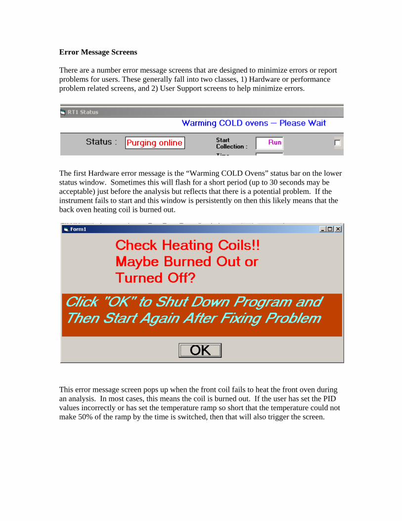
Error Message Screens There are a number error message screens that are designed to minimize errors or report problems for users. These generally fall into two classes, 1) Hardware or performance problem related screens, and 2) User Support screens to help minimize errors.
The first Hardware error message is the “Warming COLD Ovens” status bar on the lower status window. Sometimes this will flash for a short period (up to 30 seconds may be acceptable) just before the analysis but reflects that there is a potential problem. If the instrument fails to start and this window is persistently on then this likely means that the back oven heating coil is burned out.
This error message screen pops up when the front coil fails to heat the front oven during an analysis. In most cases, this means the coil is burned out. If the user has set the PID values incorrectly or has set the temperature ramp so short that the temperature could not make 50% of the ramp by the time is switched, then that will also trigger the screen.
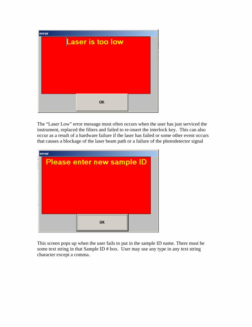
The “Laser Low” error message most often occurs when the user has just serviced the instrument, replaced the filters and failed to re-insert the interlock key. This can also occur as a result of a hardware failure if the laser has failed or some other event occurs that causes a blockage of the laser beam path or a failure of the photodetector signal
This screen pops up when the user fails to put in the sample ID name. There must be some text string in that Sample ID # box. User may use any type in any text string character except a comma.
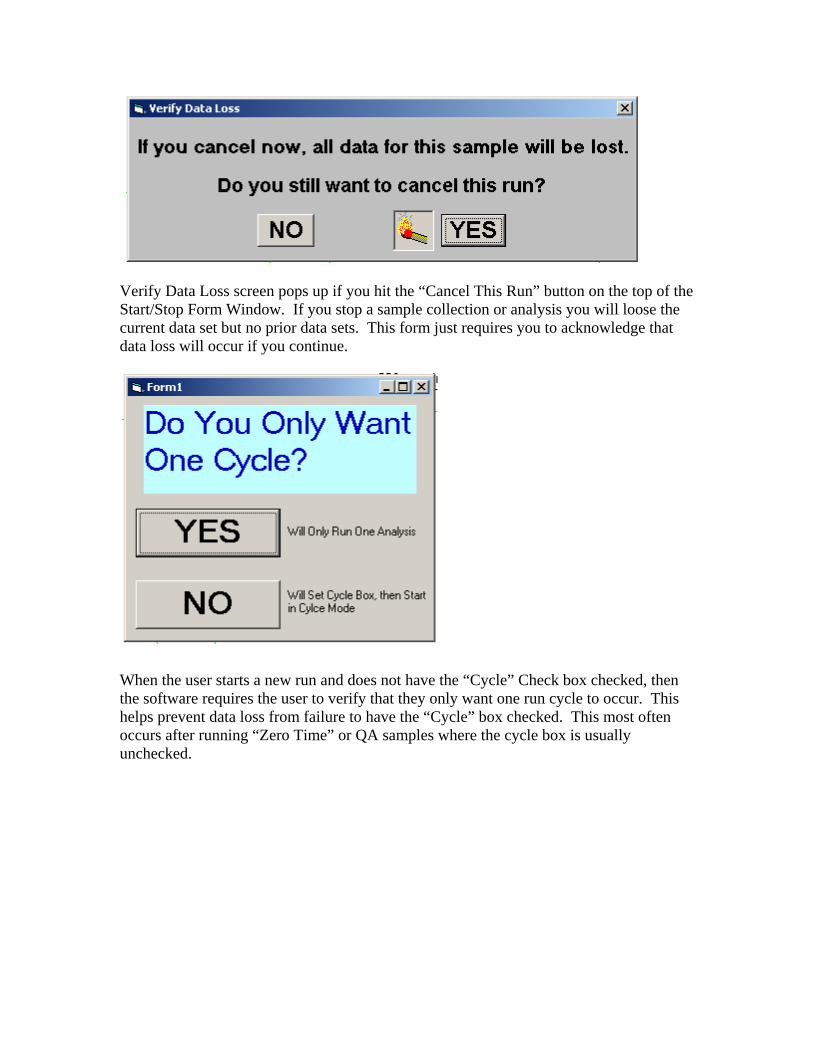
Verify Data Loss screen pops up if you hit the “Cancel This Run” button on the top of the Start/Stop Form Window. If you stop a sample collection or analysis you will loose the current data set but no prior data sets. This form just requires you to acknowledge that data loss will occur if you continue.
When the user starts a new run and does not have the “Cycle” Check box checked, then the software requires the user to verify that they only want one run cycle to occur. This helps prevent data loss from failure to have the “Cycle” box checked. This most often occurs after running “Zero Time” or QA samples where the cycle box is usually unchecked.
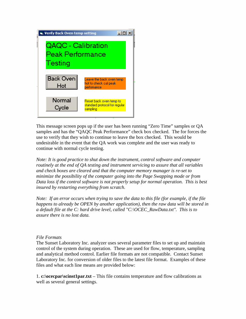
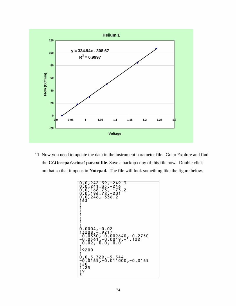
This message screen pops up if the user has been running “Zero Time” samples or QA samples and has the “QAQC Peak Performance” check box checked. The for forces the use to verify that they wish to continue to leave the box checked. This would be undesirable in the event that the QA work was complete and the user was ready to continue with normal cycle testing. Note: It is good practice to shut down the instrument, control software and computer routinely at the end of QA testing and instrument servicing to assure that all variables and check boxes are cleared and that the computer memory manager is re-set to minimize the possibility of the computer going into the Page Swapping mode or from Data loss if the control software is not properly setup for normal operation. This is best insured by restarting everything from scratch. Note: If an error occurs when trying to save the data to this file (for example, if the file happens to already be OPEN by another application), then the raw data will be stored in a default file at the C: hard drive level, called "C:\OCEC_RawData.txt". This is to assure there is no lost data. File Formats The Sunset Laboratory Inc. analyzer uses several parameter files to set up and maintain control of the system during operation. These are used for flow, temperature, sampling and analytical method control. Earlier file formats are not compatible. Contact Sunset Laboratory Inc. for conversion of older files to the latest file format. Examples of these files and what each line means are provided below: 1. c:\ocecpar\scinst1par.txt – This file contains temperature and flow calibrations as well as several general settings.
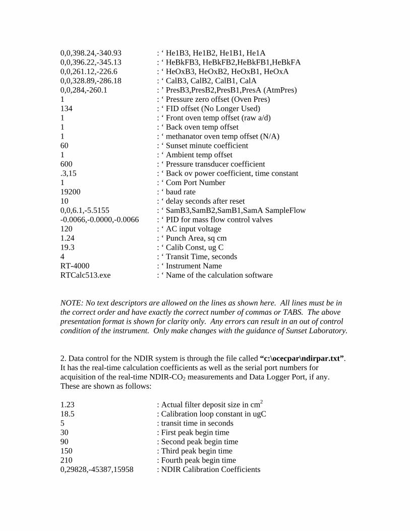
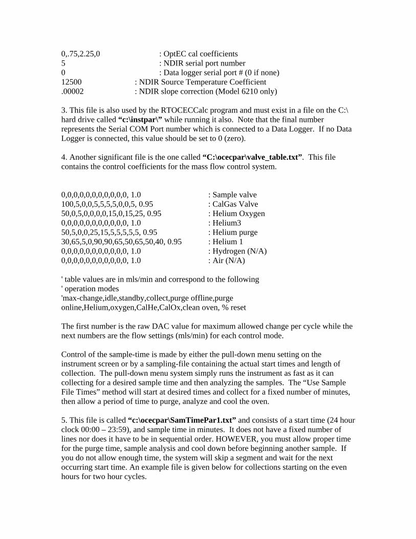
0,0,398.24,-340.93 : ‘ He1B3, He1B2, He1B1, He1A 0,0,396.22,-345.13 : ‘ HeBkFB3, HeBkFB2,HeBkFB1,HeBkFA 0,0,261.12,-226.6 : ‘ HeOxB3, HeOxB2, HeOxB1, HeOxA 0,0,328.89,-286.18 : ‘ CalB3, CalB2, CalB1, CalA 0,0,284,-260.1 : ’ PresB3,PresB2,PresB1,PresA (AtmPres) 1 : ‘ Pressure zero offset (Oven Pres) 134 : ‘ FID offset (No Longer Used) 1 : ‘ Front oven temp offset (raw a/d) 1 : ‘ Back oven temp offset 1 : ‘ methanator oven temp offset (N/A) 60 : ‘ Sunset minute coefficient 1 : ‘ Ambient temp offset 600 : ‘ Pressure transducer coefficient .3,15 : ‘ Back ov power coefficient, time constant 1 : ‘ Com Port Number 19200 : ‘ baud rate 10 : ‘ delay seconds after reset 0,0,6.1,-5.5155 : ‘ SamB3,SamB2,SamB1,SamA SampleFlow -0.0066,-0.0000,-0.0066 : ‘ PID for mass flow control valves 120 : ‘ AC input voltage 1.24 : ‘ Punch Area, sq cm 19.3 : ‘ Calib Const, ug C 4 : ‘ Transit Time, seconds RT-4000 : ‘ Instrument Name RTCalc513.exe : ‘ Name of the calculation software NOTE: No text descriptors are allowed on the lines as shown here. All lines must be in the correct order and have exactly the correct number of commas or TABS. The above presentation format is shown for clarity only. Any errors can result in an out of control condition of the instrument. Only make changes with the guidance of Sunset Laboratory. 2. Data control for the NDIR system is through the file called “c:\ocecpar\ndirpar.txt”. It has the real-time calculation coefficients as well as the serial port numbers for acquisition of the real-time NDIR-CO2 measurements and Data Logger Port, if any. These are shown as follows: 1.23 : Actual filter deposit size in cm2 18.5 : Calibration loop constant in ugC 5 : transit time in seconds 30 : First peak begin time 90 : Second peak begin time 150 : Third peak begin time 210 : Fourth peak begin time 0,29828,-45387,15958 : NDIR Calibration Coefficients
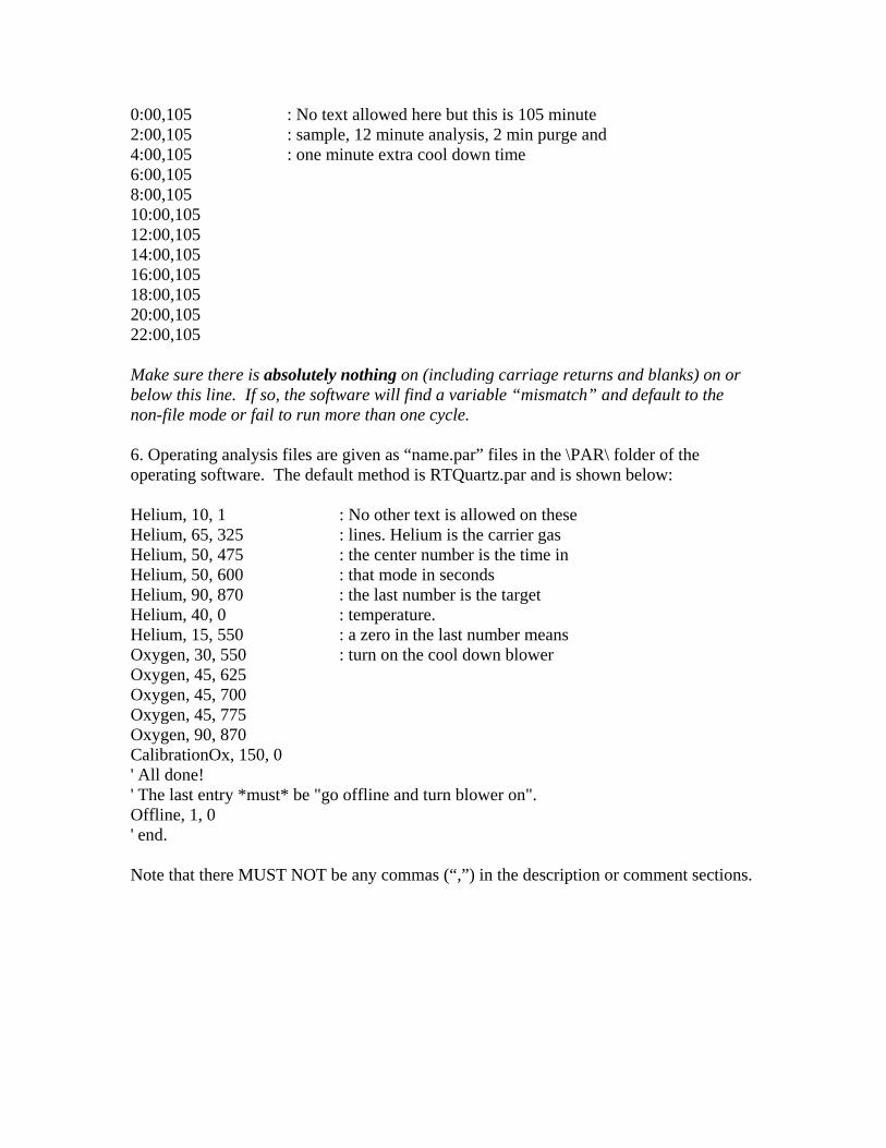
0,.75,2.25,0 : OptEC cal coefficients 5 : NDIR serial port number 0 : Data logger serial port # (0 if none) 12500 : NDIR Source Temperature Coefficient .00002 : NDIR slope correction (Model 6210 only) 3. This file is also used by the RTOCECCalc program and must exist in a file on the C:\ hard drive called “c:\instpar\” while running it also. Note that the final number represents the Serial COM Port number which is connected to a Data Logger. If no Data Logger is connected, this value should be set to 0 (zero). 4. Another significant file is the one called “C:\ocecpar\valve_table.txt”. This file contains the control coefficients for the mass flow control system. 0,0,0,0,0,0,0,0,0,0,0, 1.0 : Sample valve 100,5,0,0,5,5,5,5,0,0,5, 0.95 : CalGas Valve 50,0,5,0,0,0,0,15,0,15,25, 0.95 : Helium Oxygen 0,0,0,0,0,0,0,0,0,0,0, 1.0 : Helium3 50,5,0,0,25,15,5,5,5,5,5, 0.95 : Helium purge 30,65,5,0,90,90,65,50,65,50,40, 0.95 : Helium 1 0,0,0,0,0,0,0,0,0,0,0, 1.0 : Hydrogen (N/A) 0,0,0,0,0,0,0,0,0,0,0, 1.0 : Air (N/A) ' table values are in mls/min and correspond to the following ' operation modes 'max-change,idle,standby,collect,purge offline,purge online,Helium,oxygen,CalHe,CalOx,clean oven, % reset The first number is the raw DAC value for maximum allowed change per cycle while the next numbers are the flow settings (mls/min) for each control mode. Control of the sample-time is made by either the pull-down menu setting on the instrument screen or by a sampling-file containing the actual start times and length of collection. The pull-down menu system simply runs the instrument as fast as it can collecting for a desired sample time and then analyzing the samples. The “Use Sample File Times” method will start at desired times and collect for a fixed number of minutes, then allow a period of time to purge, analyze and cool the oven. 5. This file is called “c:\ocecpar\SamTimePar1.txt” and consists of a start time (24 hour clock 00:00 – 23:59), and sample time in minutes. It does not have a fixed number of lines nor does it have to be in sequential order. HOWEVER, you must allow proper time for the purge time, sample analysis and cool down before beginning another sample. If you do not allow enough time, the system will skip a segment and wait for the next occurring start time. An example file is given below for collections starting on the even hours for two hour cycles.
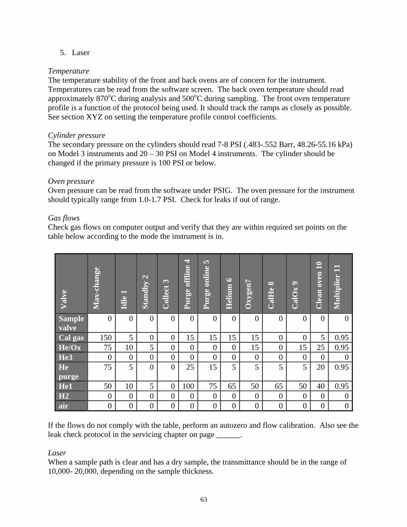
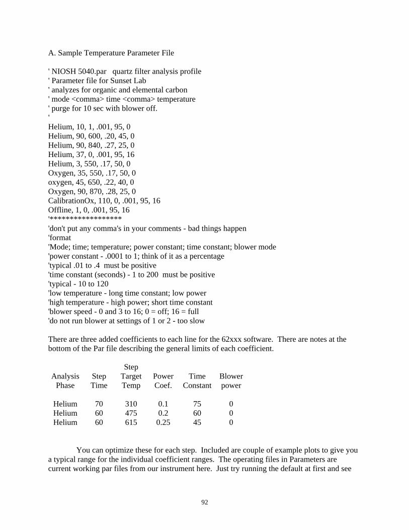
0:00,105 : No text allowed here but this is 105 minute 2:00,105 : sample, 12 minute analysis, 2 min purge and 4:00,105 : one minute extra cool down time 6:00,105 8:00,105 10:00,105 12:00,105 14:00,105 16:00,105 18:00,105 20:00,105 22:00,105 Make sure there is absolutely nothing on (including carriage returns and blanks) on or below this line. If so, the software will find a variable “mismatch” and default to the non-file mode or fail to run more than one cycle. 6. Operating analysis files are given as “name.par” files in the \PAR\ folder of the operating software. The default method is RTQuartz.par and is shown below: Helium, 10, 1 : No other text is allowed on these Helium, 65, 325 : lines. Helium is the carrier gas Helium, 50, 475 : the center number is the time in Helium, 50, 600 : that mode in seconds Helium, 90, 870 : the last number is the target Helium, 40, 0 : temperature. Helium, 15, 550 : a zero in the last number means Oxygen, 30, 550 : turn on the cool down blower Oxygen, 45, 625 Oxygen, 45, 700 Oxygen, 45, 775 Oxygen, 90, 870 CalibrationOx, 150, 0 ' All done! ' The last entry *must* be "go offline and turn blower on". Offline, 1, 0 ' end. Note that there MUST NOT be any commas (“,”) in the description or comment sections.
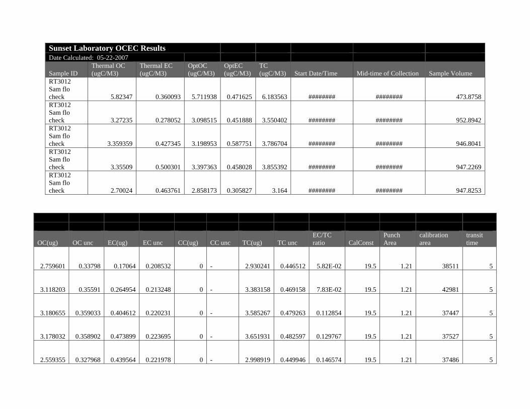
Data Analysis The purpose of this section is to provide information on the OC/EC analysis program, assist in determining what values are appropriate, and provide remedial action for problems. OC/EC Analysis Program The Sunset Laboratory OC/EC Analysis Program is used to calculate the results from a sample set after the data are stored under the base file name. The data are summed over the range to yield the total carbon results. The overall carbon response is based on a multi-point external calibration. The external methane standard for every cylinder is calibrated against the external multi-point calibration. The external methane standard is run at the end of every sample. This known amount is used to normalize the response factor for each sample. This essentially cancels out small drifts in detector response over time. The software determines an initial NDIR response baseline prior to the desorption and analysis. The area at each point along the thermogram curve minus the baseline is multiplied against the calibration response to determine the carbon. The automated OC/EC split point is calculated from where the laser absorbance in the oxidizing phase of the EC analysis matches the initial absorbance measured when the sample was first inserted into the oven. Carbon observed before the split point is considered organic carbon and carbon after the split is considered elemental carbon. The analyst has several options in computing the results from a set of experiments. These should be exercised with caution based on the extent of the analyst’s experience. The analysis program can batch process all of the sample data sets in a file without further review. It is recommended that the analyst study each individual data set as it is processed to look for any anomalies. During the processing, the analyst can calculate carbonate (if evolved as a single peak) by using the manual integration feature in the program. When re-integrating, the program draws a baseline between the designated points and calculates the peak area. The program will then automatically call this area carbonate and subtract it from the initial area for organic carbon (which includes carbonate, if present). There is no option for validating the presence of carbonate (as there is with integrated sample filters) because all of the sample is consumed during the analysis. If necessary, the OC/EC split point can be manually set (reassigned) by moving the cursor to the desired point. The software will calculate the split based on that point. This decision is based on the analyst’s experience and information about the sample. Method 1. Click on the designated calculation software file RTCalcxxx.exe. This can be found in
the primary control software folder on the C drive or the shortcut Icon on the
Desktop.
2. The software will automatically open the raw data folder. Select a sample file to be
analyzed. An uncalculated sample will be specified as the samplename.txt at the
end.
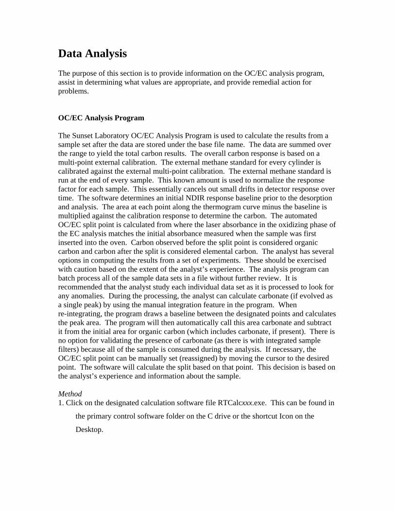
3. Selecting a sample will then open up the OC/EC analysis program.
4. On the left-hand side of the screen is the icon that is shown below. From here, the split
point can be changed, the scale factors can be changed, the sample can be
calculated, the sample can be printed, and all of the samples can be calculated.
5. Once the specifications are adjusted, press calculate sample. A screen will come up
that looks like below.
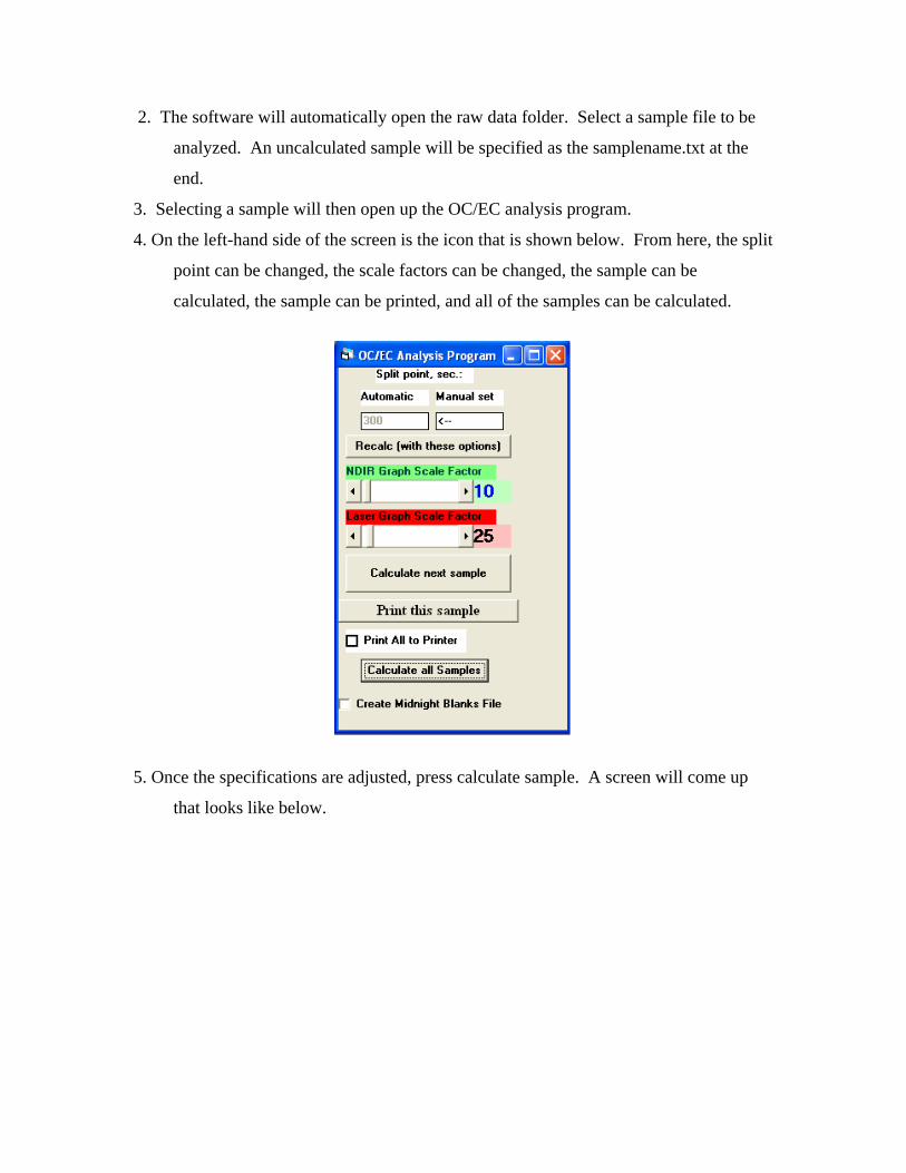
6. If there is carbonate in the sample, the results can be changed to accommodate this.
Place the cursor in the start box and press the right arrow. This will cause a dotted
line to move to the right. Move this line until the beginning of the desired curve.
Then place the cursor in the end box and press the left arrow until the second dotted
line moves to the end of the curve desired. When the curve of carbonate is enclosed
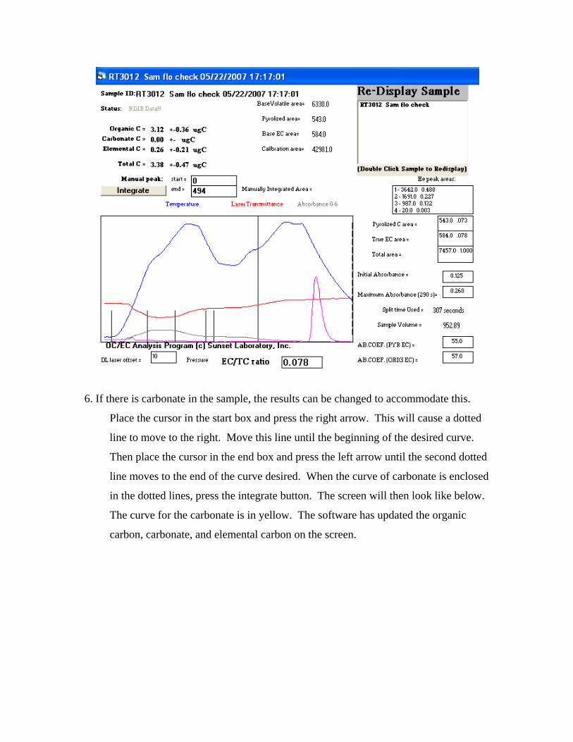
in the dotted lines, press the integrate button. The screen will then look like below.
The curve for the carbonate is in yellow. The software has updated the organic
carbon, carbonate, and elemental carbon on the screen.
7. Once a sample set has been calculated, the results can be found in the instrument’s
main subfolder on the C drive. Click on the raw data file. Under the raw data file,
there will be sample sets with different specifications at the end. For each sample
set there are four different files: thesamplesetname.txt,
thesamplesetname_BlanksRes.txt, thesamplesetname_MinuteEC.txt, and
Column Name Column Description Sample ID Name of sample Thermal OC (ugC/M3) Amount of thermal organic carbon Thermal EC (ugC/M3) Amount of thermal elemental carbon OptOC (ugC/M3) Amount of optical organic carbon TC (ugC/M3) Amount of total carbon Start Date/Time Date and time at which sample started running Mid-time of Collection
Time in which the collection is halfway
Sample Volume Volume of sample OC(ug) Amount of organic carbon OC unc Organic carbon uncertainty EC(ug) Amount of elemental carbon EC unc Elemental carbon uncertainty CC(ug) Amount of carbonate carbon CC unc Carbonate uncertainty TC(ug) Amount of total carbon TC unc Total carbon uncertainty EC/TC ratio ratio of the Total carbon the elemental carbon. Indicative of
the degree of diesel in the sample
CalConst constant for the methane carbon in the fixed calibration loop Punch Area Area of your filter punch calibration area Area of the calibration peak transit time time in seconds determined for the individual instrument as
the time offset between the laser signal (which is essentially real time and the FID signal which occurs after the sample carbon transits through the oxidizer oven, methanator oven and associated tubing. The FID results are shifted in time that many seconds so that the data correspond to the observed laser signal.
Split time(sec) laser computed split time between OC and EC
Manual split?(sec) split time that can be set by the analyst if they choose Init.Abs. Apparent absorbance based on the initial laser signal and
final laser signal after analysis Abs.Coef. Apparent absorption coefficient of the EC on the filter based
on the Thermally measured EC and the Initial Abs.
Atm.Pres.mmHg local apparent atmospheric pressure at the time of analysis
60
OCPk1,ug C/cub m OCPk2,ug C/cub m OCPk3,ug C/cub m OCPk4,ug C/cub m
The Peaks are based on the area under the peak during each of 4 temperature ramps under helium. Some people claim they can get source data from evaluating the peak ratios
Pyrolized C/cub m carbon associated with Pyrolysis as determined by the laser split point
True EC/cub m Optical EC (ugC) Apparent EC on the filter based on a fixed absorption
coefficient and the apparent absorbance (init Abs)
OptEC ABS Apparent absorbance based on the initial and final laser reading during the thermal analysis
OptABS Coef Absorption coefficient calculated from the absorbance the calculated elemental carbon
Opt Coef X^3 Coefficient for the polynomial fit of the Optical EC Opt Coef X^2 Coefficient for the polynomial fit of the Optical EC Opt Coef X^1 Coefficient for the polynomial fit of the Optical EC Opt Coef X^0 Coefficient for the polynomial fit of the Optical EC CO2_ndirC3 Coefficient for the polynomial fit of the NDIR CO2_ndirC2 Coefficient for the polynomial fit of the NDIR CO2_ndirC1 Coefficient for the polynomial fit of the NDIR CO2_ndirC0 Coefficient for the polynomial fit of the NDIR Laser Correction Correction factor based on the laser attenuation as a function
of heating. Begin Int - beginning integration point
Acceptance Criteria
Parameter Number Limit Single point external standards 1 per week Calculated ± 5.0 % Instrument blanks 1 per week Value ± 0.3 µg C Multipoint external standard set 1 per 100 samples Calculated ± 5.0 %
61
Remedial Action External standard out of range - carefully prepare and re-run two standards. If standards are still uniformly out range then:
Check gas flows (see maintenance
chapter on page ____) Check for leaks (see servicing
chapter on page _____) Check system temperatures (see
maintenance chapter on page ____) Re-make stock solution. Re-run
samples (See operation chapter on page ____)
Perform multipoint calibration and update calibration parameter file (see calibration chapter on page ____)
Check for leaks (see servicing chapter on page ____)
Check system pressure (see maintenance chapter on page ____)
Check oxygen trap (see servicing section on page ____)
Check gas lines to be sure no Teflon is used
External methane standard out of range
Check carrier gas flow rates.
Recalibrate if necessary (see maintenance chapter on page ____)
Check system pressure (see maintenance section on page ____)
Check for leaks (see servicing chapter on page ____)
62
Maintenance The purpose of this section is to supply you with information that will help keep the instrument in top condition. The information provided includes a maintenance timeline, routine inspections, sample filter replacement, denuder filter replacement, cleaning cyclone protocol, and flow sensor calibration. The instrument requires virtually no routine maintenance over extended periods of time. Proper care of the instrument will result in reliable performance and an extended lifetime. For warranty information see appendix. Maintenance Timeline Daily
Check the instrument for error flags that show hardware problems
Weekly Run calibration check (for protocol see
calibration chapter on page ____) Replace sample filters (see protocol on
page____) Routine inspections (see section on page
____)
Monthly Replace denuder filters (see protocol on
page ____) Clean Cyclone (see protocol on page ____)
Semi-annual Re-calibrate flow sensors (see protocol on
page ____) Clean sample inlet components (See
section on page____)
Routine Inspections The instrument should be checked regularly for:
1. Temperature stability 2. Gas Cylinder pressure 3. Oven pressure 4. Carrier Gas flows (autozero weekly)
63
5. Laser Temperature The temperature stability of the front and back ovens are of concern for the instrument. Temperatures can be read from the software screen. The back oven temperature should read approximately 870oC during analysis and 500oC during sampling. The front oven temperature profile is a function of the protocol being used. It should track the ramps as closely as possible. See section XYZ on setting the temperature profile control coefficients. Cylinder pressure The secondary pressure on the cylinders should read 7-8 PSI (.483-.552 Barr, 48.26-55.16 kPa) on Model 3 instruments and 20 – 30 PSI on Model 4 instruments. The cylinder should be changed if the primary pressure is 100 PSI or below. Oven pressure Oven pressure can be read from the software under PSIG. The oven pressure for the instrument should typically range from 1.0-1.7 PSI. Check for leaks if out of range. Gas flows Check gas flows on computer output and verify that they are within required set points on the table below according to the mode the instrument is in.
If the flows do not comply with the table, perform an autozero and flow calibration. Also see the leak check protocol in the servicing chapter on page ______. Laser When a sample path is clear and has a dry sample, the transmittance should be in the range of 10,000- 20,000, depending on the sample thickness.
1. Open filter access port using the finger tight nuts on the door panel.
2. Remove laser shroud by pulling up on back on the panel.. This shroud acts as a
protective housing for the oven port preventing exposure to the laser system. It has a
keyed interlock system which automatically shuts down the laser upon access to this area.
65
3. To remove the photodetector, remove the stainless steel nut and then loosen the nylon nut
with hands. Gently slide the photodetector off the quartz insert. Avoid excess force as
the quartz oven can be easily chipped or broken if caution is not observed.
4. Place the photodetector on the oven plate.
66
5. Push the filter removal tool through the filter and pull it out concurrently with the insert.
6. Using filter punch, cut a new 17mm quartz filter.
7. Using the flat-faced forceps, gently insert the new filter into the oven port perpendicular
to the tube inlet about ¼”. Using the forceps, gently rotate the filter using care not to
puncture or bend it. Slide in the filter with the insert at least 1 inch and then install a
second filter. It does NOT have to be completely square or rotated in the oven port at this
time.
67
8. Wipe the quartz insert with a clean Kim-Wipe or other lint-free cloth to remove any
fingerprints, lent or filter fragments which may be present on the insert.
9. Slide insert in parallel to the oven observing the filter as it begins to square up with the
face of the insert and slide into the port. It will offer mild resistance to being pushed into
the port. However, RESIST ALL URGES TO FORCE any aspect of this job. If it does
not slide in easily, slip it out and start over. As the insert slides farther into the port, it
will press the filter against the seat in the heated zone. Once you can feel the filter begin
to seat, hold the insert firmly against the filter and hand-tighten the fitting nut securing it
in place. The most critical period for accidentally breaking or chipping the insert is
during the first ½ - 1” of insertion as the piece makes contact with the filter but still can
be twisted or rotated off-axis with the oven port. Once the piece has been slid in far
enough to limit this motion, the chances for breakage are significantly reduced.
68
10. Reinstall the photodetector making sure the face of the o-ring is in place before
reinstalling. The fittings should be tightened using hands.
11. Reinstall the laser shroud
Injection Port Septum The gas injection port is used for syringe injection of gas standards for QAQC performance monitoring of the instrument. Early instruments simply used a Swageloc nut and GC septum on the port while later instruments included a needle guide. The needle guide greatly improved the overall performance and reduced leaks from the septum. All users are encouraged to contact Sunset Laboratory Inc. for the needle guide upgrade. The septum should be replaced after every 10 injections or if there is any evidence of a leak. The most obvious indication of a leak is if you note a significant drop in the instrument pressure when inserting or removing the syringe needle during an injection. The septa are ¼” OD GC septa and can be purchased in bulk from Restek (Part No. 27128). The needle guide can be obtained from Sunset Laboratory Inc. Materials New septa Needle guide insert Small screwdriver Method
1. Shut down the instrument software 2. Remove the Swageloc nut and septum from the injection port 3. Use the small screwdriver to pry out the septum 4. Make sure that the needle guide in correctly inserted into the Swageloc nut with the guide
tip in the hole and the flat surface facing the septum. 5. Carefully insert the septum so that it remains squarely in the nut.
69
6. Screw the nut back onto the port until you just feel the septum begin to seat on the face of the port. Turn an additional ½ turn. Do not over tighten the nut as this will cut and core out the septum causing it to fail quickly
Replacing Denuder Filters Under continuous use, Sunset Laboratory Inc. recommends that the parallel plate filters be changed at least once a month to minimize the possibility of VOC breakthrough. If an increase above typical adsorbed VOC is observed on quartz backup filters, then the carbon filters should be changed immediately. Filter sets are available from Sunset Laboratory Inc. or they can be cut as needed by the customer. The bulk filter material is supplied by Schleicher and Scheull, Inc., Reference Number 10320163, Phone Number 1-800-645-2302. The strips can be cut with a good quality paper cutter to the dimensions of 1.25” x 8.0” (The bulk material is 8” x 10” so a 1.25” wide strip can be cut from the 8” side minimizing the number of cuts necessary to produce the desired size.). Fifteen strips are necessary for each replacement set. Materials Philips head screwdriver New filter material Method
1. To change the filters, remove the denuder from the sample train and place on a flat
surface.
2. Unscrew the front plate and set aside on the table.
3. Slide out the parallel plate insert tray and place on the table.
4. The filter plates are stacked in the tray and separated by 2 mm spacer rods. Remove all
of the filters and spacers.
5. Discard the old filter material.
6. Install the new filter strips in the reverse order separating each with a spacer rod on each
side. Be sure to place a strip in the bottom of the tray against the aluminum surface and
last strip at the top of the tray so that when it is re-inserted into the denuder that there is
no exposed aluminum surface in the parallel plate sector of the denuder.
7. Carefully re-insert the tray being sure that the top filter is not dislodged as the tray slides
into the outer shell. Also be sure that the flow direction indicated matches the outside
direction arrow.
70
8. Re-attach the front cover with the o-ring properly seated. When tightening the screws,
assure that they are uniformly tightened to affect a good seal. The end plate does not
have to be so tight that it contacts the outer shell.
Cleaning Cyclone and Inlet tubing The sampling inlet of all sampling systems needs to be cleaned periodically. The cyclone inlet accumulates the larger particles from the sample air stream. There are also some vapor phase losses to the walls of the cyclone and connective tubing. All of this must be cleaned periodically (6 months) to minimize high blanks and adsorbed vapor artifacts. Materials 1/8” Allen wrench Methanol, acetone or methylene chloride small brush such as a gun cleaning brush and cloth clean, high pressure air or nitrogen source Method
1. Remove cyclone from sample inlet by pulling it. Be careful not to damage the o-rings.
2. Lift the rain hat off the cyclone.
3. Unscrew the dust port
4. Disassemble the cyclone body by removing the three screws using Allen wrench.
5. Take small brush, methanol, or high pressure device and clean the body
6. Reassemble
7. Disassemble the tubing.
8. Rinse with methanol
9. If possible, swab with a brush or cloth
10. Blow dry with high pressure clean air or nitrogen. Even better, heat with a heat gun
while flushing with gas.
11. Reassemble everything.
Flow Sensor Calibration Flow sensor calibration is multi-step process which must be performed in the correct order. If performed properly and the data logged correctly into the instrument parameter file, the observed flow reading on the flow table should be correct (± 5 %) for an extended period. The instrument will come with an initial flow calibration from the factory. Initial offsets and a calibration check
71
will be performed on-site by the Sunset Laboratory Engineer. Because the sensors work using the carrier gas heat capacity and have been exposed to air during shipment, the initial calibration may change over the course of the first week or so of operation. Thus, the flows should be re-calibrated after the system has been given sufficient time to burn in. Flow sensor re-calibration should be preformed once a year. Flow calibration measurements should be made with a NIST traceable gas flow measurement such as an electronic bubble meter, GilibratorTM, or other reputable manufacturer’s flow meter. Record all data in a dated instrument log. Materials Flow meter “C:\ocecpar\scinst1par.txt” file Swageloc 1/8” fitting “Cal Data” worksheet Instrument log Method
1. Turn on each of the support gas cylinders and set the secondary regulators to
approximately 10-15 PSI. Flows are controlled by electronic flow controllers. The
system will automatically try to control the flows to the system setpoints. Observe the
flow table for each of the gases as they settle into a constant flow. Note: The flow
sensors are sensitive instruments! Keep the secondary pressures at the recommended
levels and make all adjustments slowly! Extreme, rapid changes in flows or very high
pressures can destroy the sensors resulting in a non-warranty repair charge!
2. Attach the gas flow meter as a Gilibrator or FlowCal device with a 1/8” fitting on the
“Back Oven Vent” port on the back of the instrument.
3. On the lower window of the software, check the “Valves” box. This will bring up the
Valves screen. Use this screen to control the flows while performing the calibrations.
72
4. You will need to collect flow vs. Voltage output from the instrument. Pull down the
bottom edge of the “Flow Table” screen and check the “Display Sensor Voltages” button.
This will bring up the actual voltage readings from the data system.
5. First get your “zero” readings. This is best done by checking the “Override DAC” box
and then moving the slider bars all the way to the left. This forces the flow control valves
shut and gives the most accurate zero reading. Record the readings for all four flow
gases on the top section of the flow table.
6. Now for the upper limit readings, uncheck the “Override DAC” box and check the
“Override flow” box. Highlight the flow in the right column for each of the flows and
type in a “0”. Now type in “100” for the He1 flow and wait for the computer to stabilize
the flow by monitoring the Voltage on the flow table. Once it appears stabile, (+- a few
millivolts), record the voltage and measure the actual flow using the flow meter on the
“Back Oven Vent”. Record the flow and the voltage.
73
7. Now type in a “0” for the He1 flow and perform the same sequence for HePurge and
HeOx recording the flow and voltage. The flow measurement is taken from the “Back
Oven Vent” for these two flows as well as the He1.
8. Move the flow meter to the “Cal Gas Vent” and repeat the flow measurements for the
He/CH4 cal gas.
9. Record your data in a spreadsheet similar to below. You may choose a multipoint
calibration as shown by recording data over a range of flows chosen using the Valve
Screen.
Helium 1 HelPurge Helium/Oxygen Calibration Gas Volts Flow (cc/min) Volts Flow (cc/min) Voltage Flow (cc/min) Voltage Flow (cc/min)
12. The first line in the file are the coefficients for He1
0,0,242.39,-249.3
Use the results for the calculated line in the graph from the spreadsheet
y = 334.94x - 308.67
to update the file coefficients by updating the first line to read:
0, 0, 334.94, -308.67
13. Update the remaining lines for the other gases as follows:
Line 1: He1
Line 2: HePurge
Line 3: He/Ox
Line 4: CalGas
Line 22: HV flow sensor
14. Make sure that there are no extraneous commas, lines or characters in the file. Save the
file under its original file name.
15. Now turn off the heated zone switch and restart the software. The new flow coefficients
will be used for controlling the flows. You can spot check the flows using the Valve
window to set individual flows and your flow meter to verify the settings in the same
manner as you did for the original calibration. If there are no problems, turn on the heated
zones and start collecting data. A flow diagram is included on the next pages for
diagnostic purposes.
76
Analytical flow system
77
Sample Flow System
78
Standard Operating Procedure (SOP) For the Analysis of Organic and Elemental Carbon
(OC/EC) Using the Sunset Laboratory Semi-Continuous Carbon Aerosol Analyzer
January 10, 2005
Sunset Laboratory Inc.
Sunset Laboratory Inc.
10180 SW Nimbus Avenue Suite J-5
Portland, Oregon 97223
79
Table of Contents I Scope and Applicability ....................................................................................................................................... 80 II Summary of Method ............................................................................................................................................ 80 III Working Definitions ...................................................................................................................................... 80 IV Health and Safety Warnings .......................................................................................................................... 80 V Procedure ........................................................................................................................................................... 81
a) General Instructions.................................................................................................................................... 81 b) Samples ......................................................................................................................................................... 81 c) Materials ...................................................................................................................................................... 81 d) Equipment .................................................................................................................................................... 82 e) Sample Collection and Analysis Procedure ............................................................................................... 82
i) OC/EC instrument startup - Setting up for data collection ............................................................... 82 VI Calibration and Audit Procedures ............................................................................................................. 83
i) Test Equipment and Materials .............................................................................................................. 83 (3) Basic Performance Calibrations ............................................................................................................ 84 VII Data Analysis - Calculations .................................................................................................................. 86 VIII Results ................................................................................................................................................. 86
IX Remedial Action .......................................................................................................................................... 87 X Instrument/Equipment Inspection, Testing, and Maintenance ............................................................... 87
a) Routine instrument inspection .................................................................................................................. 87 b) Testing ...................................................................................................................................................... 87
c) Maintenance .................................................................................................................................................. 88 Pre-start checklist - New Installation ............................................................................................................... 94
This SOP describes the analytical method to determine the levels of organic and elemental carbon in particulates collected using the Sunset Laboratory semi-continuous carbon aerosol analyzer (RT-OCEC). The particulate samples are collected by the instrument using a predetermined sample schedule and analyzed by a thermal/optical method. Time resolution of 30 minutes to 8 + hours are possible.
III Summary of Method
A quartz filter is mounted in the quartz oven and samples are collected for the specified time. After the sample is collected, the system closes off the sample port, purges the analytical flowpath with helium and performs the thermal/optical analysis. The thermally removed carbon components are converted to CO2 which is subsequently measured by non-dispersive infrared (NDIR). External sucrose solution and methane gas carbon standards are used for NDIR calibration. Correction for the pyrolytically generated carbon (char) that sometimes forms during the first stage of the analysis is based on filter absorbance measurements. The pyrolysis step is facilitated using a laser absorbance technique.
IV Working Definitions
Organic Carbon (OC) - Optically transparent carbon removed (through thermal desorption or pyrolysis) and char deposited when heating a filter sample to a preset maximum (840 C) in a non-oxidizing (helium) carrier gas.
Elemental Carbon (EC) - Carbon (e.g., in soot particle cores) that can only be removed from the filter under an oxidizing carrier gas (He/O2). Optically absorbing carbon removed at high temperatures (e.g. 850 C ) in a non-oxidizing carrier gas when internal (sample matrix) oxidants are present.
V Health and Safety Warnings
The Sunset Laboratory Thermal/Optical Carbon Analyzer uses high temperatures (up to 870C) and laser radiation to perform the required steps in this analytical procedure. Under normal operation, the analyst is protected from exposure to these energy sources. However, during repair or trouble shooting, when the instrument cover is removed, the analyst must take the following precautions:
a) Before attempting any repairs, turn off the power and wait for all heated zones to cool.
b) For most repair work, unplug power to the ovens and avoid contact with any power sources in the oven cabinet.
81
c) Although the laser source has an interlock protection system, if the interlock is overridden, direct exposure to the laser can occur under certain conditions. Do not look directly at the laser source as permanent eye damage can occur.
d) Use caution when handling all support gas cylinders and regulators. Always have cylinders properly chained to a safety rack.
VI Procedure
a) General Instructions
See the attachment – “Installation Notes” for basic installation and operation procedures
b) Samples
The analyzer is deployed to the field site. It collects airborne particulate samples on an internally mounted filter and analyzes the sample on a semi-continuous basis. There is no option for replicates without a second sampler. Sample data are stored in raw data files. Additionally, a short result file is printed to a file at the end of each analysis. An optional output can also be transmitted to a data logger equipped with a serial input. The data should be considered irreplaceable and should be backed up on a frequent basis to some sort of permanent media such a CD-rom or tape.
c) Materials
See Table 1 for all required reagents and gases. Check the labels carefully to ensure that they are not expired and are of the proper purity/grade. Document the supplier, grade/purity and Lot No. as appropriate on the Analysis Data Form.
Table 1. Materials
Material
Use
UHP Helium (99.999%)
Carrier gas
Helium/Oxygen Mix (10% O2; balance UHP He)
EC oxidant carrier gas
Helium/Methane (5.0% methane; UHP He balance)
External standard gas
Sucrose (99.9% reagent grade)
Analytical standard
82
d) Equipment
See Table 2 for all required major pieces of equipment. Check calibration of all equipment requiring calibration to ensure that it is current.
Table 2. Equipment
Equipment
Use
Forceps Filter installation
Clean quartz filters Work area preparation
Filter punch tool (1.6 cm diameter circle) Preparing sample filters
Filter removal tool Periodic replacement of filters
10 l analytical syringe Calibration
Volumetric Flasks, Class A. Standard preparation
Analytical balance Standard preparation
e) Sample Collection and Analysis Procedure
This procedure includes default instrument setup, standards preparation as well as general operation of the Sunset Laboratory RT-OCEC analyzer. It is assumed that the analyst has experience with the routine operation of the instrument.
i) OC/EC instrument startup - Setting up for data collection
(1) Check cylinders for sufficient volume and pressure. (2) Turn ON computer be sure that the serial port cables are installed correctly and
the software configured correctly. (3) Turn on both switches on the back of the instrument. (4) Start the RT Program by double clicking (5) Make sure the computer and instrument CPU link up. Note the temperature boxes
and the flows on the flow table. They should start changing as the instrument stabilizes after startup.
(6) Check the instrument gas flows on the table to be sure they are stable. (7) Check the instrument pressure to be sure it is normal (0.5 to 1.5 psi; instrument
dependent) (8) Install new filters if necessary. (9) Run a “CLEAN OVEN” procedure from the Pull down menu if a new filter has
been installed. (10) Enter a sample name.
83
(11) Select the proper parameter file to be used for analysis. By default it is “rtquartz.par”.
(12) If you desire the raw data to go into an automatically generated file each day, the default ending of “\” is already selected. To have the data go into a file of another name, type the name of the file after the “\” already there. Be sure and end the filename with the extension “txt”( example: yourfilename.txt)
(13) Determine how the instrument will be cycled; either by sampling for a fixed time followed by the analysis; or by starting sampling times and pre-determined times and lengths from an external file.
(14) Make sure the Cycle Box is checked for continuous operation. (15) Click on “Start”
VII Calibration and Audit Procedures
Calibration and Audit procedures are related in that each is designed to check the instrument performance. Calibration measurements are performed to set up critical instrument performance parameters while Audit measurements are more routine measurements performed to assure the instrument is operating within a desired specification. Many of the techniques and procedures are similar.
i) Test Equipment and Materials
(1) Preparation of Carbon Standard Stock Solution
(a) Weigh 10.00 ± 0.01 g of sucrose on the analytical balance and quantitatively
transfer it into a 1 liter volumetric flask. Dissolve in and dilute to volume with DDi H2O. Record in the laboratory notebook. This will serve as the general QA/QC performance standard. Concentration = 4.207 g C/l solution. Note the date and replace every 6 months. Pour about 20 mL of the standard into a clean glass vial (with Teflon cap liner) and place the rest in the refrigerator.
(b) For a “low-level” working standard, make a 1 to 4 dilution in a volumetric flask with DDI H2O. This solution has 1.05 µgC/µl of solution and is used for the lowest concentration standard of a multi-point calibration. Note the date and replace every 6 months. Pour about 20 mL of the standard into a clean glass vial (with Teflon cap liner) and place the rest in the refrigerator.
(2) External Standard
The external standard is the mixed helium/methane cylinder noted in Table 1. Methane in a sample loop is automatically injected at the end of every analysis. The analytical result is normalized to the response of the methane standard to adjust for slight variations in flow rates that might occur during the day. At 760 torr and 298 K, a 5.00% methane in helium mixture contains 24.54 g of carbon per ml of gas.
84
(3) Basic Performance Calibrations
The Sunset Laboratory OC/EC instrument is calibrated during the initial installation using a multipoint external standard calibration. The external standard calibration is used to determine the carbon in the external standard gas loop. The external standard carbon content is dependent on the volume of the loop (nominally 0.8 ml) and the concentration of methane in the methane/helium tank standard. Once the standard loop carbon in determined, a parameter file is set up containing (among others) three calibration parameters; 1) the measured deposit area, 2) the calibration constant which is the number of µg carbon in the loop specific to the cylinder of helium/methane mix provided at the site, and 3) the transit time which is the time required for methane generated from a sample to reach the NDIR. These parameters are often stable for many months. External standards should be run according to program requirements with results monitored on a control chart. See sections on Acceptance Criteria and Remedial Action when the external standard responses fall out of accepted range.
(a) External Standard Loop Calibration using the stock sucrose solution
(i) Punch out three new, clean 16 mm diameter filter sections of quartz filter with the circular filter punch.
(ii) Insert 2 of the filters in the oven as required for a normal analysis cycle. Place the third filter horizontally in the quartz tube insert as close to the end as possible so that it will be in close proximity to the 2 vertically mounted filters. Re-install the insert and photodetector as required for a normal analysis.
(iii)Go to the “Run” Pull-down Menu and left-click on the Clean Oven cycle to completely clean the filter punches.
(iv) Wait for the instrument to complete the clean cycle and the status window to read “Safe the put in a new Sample”
(v) Expand the lower status window to full screen and check the “QAQC Peak Performance” Box. This will set the back oven to a constant value during the calibration testing. You will be asked to verify this setting each time you run a sample.
(vi) Go to the top Start Window and un-check the “Cycle” box and set the sample time to “0”.
(vii) Go to the “Parameter File” field and select sucrose-TC.par from the PAR folder.
(viii) Using the precision syringe, measure a sample volume of from 5 - 10 l of the standard carbon (sucrose) solution.
(ix) Remove the photodetector head and slide out the quartz insert. (x) Carefully apply the solution on the filter suspended in the quartz insert.
Re-install the quartz insert and photodetector promptly. Use caution so as not to contaminate the insert or quartz filter. Record the exact volume of the aliquot in the log book.
(xi) Go to the user interface field that is labeled “Output Raw Data file” and type a new name for the raw data file.
85
(xii) In the “Sample ID” field in the top “Start” window, type in the expected carbon loading.
(xiii) Start the analysis. Wait for the instrument to run through its analysis protocol and return to the Idle mode and safe to put in a new sample.
(xiv) Analyze a range of samples as required for the calibration. A typical multi-point calibration for ambient filters would include; 1. A 10 µl sample from the “low-level” working standard yielding 10.5
µg carbon. 2. A 5 µl sample from the standard carbon stock solution yielding 21.03
µg carbon. 3. A 10 µl sample from the standard carbon stock solution yielding 42.07
µg carbon.
(b) External Standard analysis using a fix volume standard gas injection. (i) Check the OC/EC oven to determine if the temperature is cool enough to
insert a sample. (Flashing green screen section on the computer monitor). (ii) Expand the lower status window to full screen and check the “QAQC Peak
Performance” Box. This will set the back oven to a constant value during the calibration testing. You will be asked to verify this setting each time you run a sample.
(iii)Go to the top Start Window and un-check the “Cycle” box and set the sample time to “0”.
(iv) Go to the “Parameter File” field and select cal-injection.par from the PAR folder.
(v) Go to the “Sample ID” field in the top and type in 1.0 ml cal gas sample. (vi) Go to the lower status window and check the “Valve Values Table”
checkbox. (vii) A new window will pop up with the gas flow controls present.
Check the “Override flows” box at the lower right of the panel. Highlight the bottom right number (Default = 5) for the flow rate of the Cal Gas. Change the value to 25 and wait for the new flow setting to stabilize.
(viii) Using a 1.0 ml gas tight syringe, collect a cal gas sample from the back “Cal Gas Vent” port.
(ix) Start the analysis. Wait for the Analyze mode and the temperature to stabilize. Inject the gas sample in a steady single motion in 1 – 2 seconds. Leave the syringe in the septum until the peak has finished eluting then remove the syringe and wait for the analysis to finish.
(x) Calculate the result and verify that the carbon measured is within (±) 5.0% of the expected total carbon.
(xi) Calculations:
Total Carbon (ugC) = (mls inj) x (% methane/100) x 12 x ( P/RT) x 1000 Where: P/RT = pressure (atm) / (.082 x Temp (K)
86
VIII Data Analysis - Calculations
a) The Sunset Laboratory OC/EC Analysis Program is used to calculate the results from a sample set after the data are stored under the base file name. The OC/EC calculation program is initiated by clicking on the icon. The program then asks for the file name to perform calculations. In general, the following software parameters apply to all calculations;
b) The overall carbon response is based on a multi-point external calibration. c) The external methane standard for every cylinder is calibrated against the external multi-
point calibration. d) The external methane standard is run at the end of every sample. This known amount is
used to normalize the response factor for each sample. This essentially cancels out small drifts in detector response over time.
e) The software determines an initial NDIR response baseline prior to the desorption. The area at each point along the thermogram curve minus the baseline is multiplied against the calibration response to determine the carbon. The data are summed over the range to yield the total carbon results.
f) The automated OC/EC split point is calculated from where the laser absorbance in the oxidizing phase of the EC analysis matches the initial absorbance measured when the sample was first inserted into the oven. Carbon observed before the split point is considered organic carbon and carbon after the split is considered elemental carbon.
g) The analyst has several options in computing the results from a set of experiments. These
should be exercised with caution based on the extent of the analyst’s experience.
h) The analysis program can batch process all of the sample data sets in a file without further review. It is recommended that the analyst study each individual data set as it is processed to look for any anomalies.
i) During the processing, the analyst can calculate carbonate (if evolved as a single peak) by using the manual integration feature in the program. This must be performed by setting the left and right cursors on the beginning and ending points of the carbonate peak. When re-integrating, the program draws a baseline between the designated points and calculates the peak area. The program will then automatically call this area carbonate and subtract it from the initial area for organic carbon (which includes carbonate, if present). There is no option for validating the presence of carbonate (as there is with integrated sample filters) because all of the sample is consumed during the analysis.
j) If necessary, the OC/EC split point can be manually set (reassigned) by moving the cursor to the desired point. The software will calculate the split based on that point. This decision is based on the analyst’s experience and information about the sample.
IX Results
a) The analysis software automatically stores the data in a spreadsheet format for compilation. The spreadsheet format is illustrated in Attachment B. The data for each sample may also be printed in graphic form with the temperature, laser absorbance, and
87
NDIR profiles. The net results are tabulated and a line is provided for the analyst’s signature. An example of this results output is provided in Attachment C.
Table 4. Acceptance Criteria
Parameter Number Limit Single point external standards 1 per week Calculated ± 5.0 % Instrument blanks 1 per week Value ± 0.3 µg C Multipoint external standard set 1 per 100 samples Calculated ± 5.0 %
X Remedial Action
a) External standard out of range - carefully prepare and re-run two standards. If standards are still uniformly out range then; i) Check gas flows ii) Check for leaks iii) Check system temperatures iv) Re-make stock solution. Re-run samples v) Perform multipoint calibration and update calibration parameter file
b) System blanks too high
i) Check for leaks ii) Check system pressure iii) Check oxygen trap iv) Check gas lines to be sure no Teflon is used
c) External methane standard out of range
i) Check carrier gas flow rates. Recalibrate if necessary ii) Check system pressure iii) Check for leaks
XI Instrument/Equipment Inspection, Testing, and Maintenance
a) Routine instrument inspection
i) Check cylinder pressures - replace as necessary ii) Observe oven pressure - check for leaks if out of typical range (1.0 - 1.7 psi). iii) Observe standby temperatures of back oven and methanator oven prior to startup. If
out of range, determine cause and initiate repair. iv) Check gas flows on computer output and verify that they are within required set
points. If out of range, look for system leaks. Repair or adjust as necessary. b)Testing
i) The instrument requires virtually no routine maintenance over extended periods of time. Breakage or failure can occasionally occur with the components described below. If breakage or failure occurs, components should be replaced as necessary with replacements from Sunset Laboratory. Sunset Laboratory has Power Point presentations available for many of the typical maintenance repair procedures.
ii) Replacement of quartz oven - the quartz oven/MnO2 converter almost never fails
except in the case of operator breakage or development of cracks. If this occurs, the oven will have to be replaced. Begin by cooling the oven to ambient and shutting off all gas flows. Unplug all electrical power. Begin disassembly by removing the thermocouple, photodetector and top cover. Next, carefully remove all insulation from the oven area. Disconnect the heating coils and carefully unwrap them from the oven assembly. Remove the top oven supports and lift out the oven. Remove the thermocouple from the back of the instrument. Remove the desorption oven thermocouple by disconnecting the Swagelok fitting. Replace in reverse order using care in installing the oven thermocouple, heating coils and insulation. Once installed, re-start gas flows to purge with helium and initiate startup sequence in the software.
iii) Replacement of heating coils - heating coils will occasionally burn out. When this happens, they will have to be replaced. Follow the replacement steps for the appropriate component above (Maintenance, Steps 1 and 2) until the coil can be removed. Replace with Sunset Laboratory replacement part. Assemble in reverse order.
89
XII References
a)NIOSH Method 5040 (1998), In NIOSH Manual of Analytical Methods (NMAM), 4th ed., 2nd Supplement, ed. Cassinelli M.E., O’Connor P.F. [Supplement to DHHS (NIOSH) Publication No. 94-113]
b)M. E. Birch, Analyst (1998), 123:851-857 c)M. E. Birch, R. A. Cary (1996) Aerosol Science and Technology, 25:221-241 d)Cass, et. Al.
90
XIII Revision History
91
XIV Attachments
92
A. Sample Temperature Parameter File ' NIOSH 5040.par quartz filter analysis profile ' Parameter file for Sunset Lab ' analyzes for organic and elemental carbon ' mode <comma> time <comma> temperature ' purge for 10 sec with blower off. ' Helium, 10, 1, .001, 95, 0 Helium, 90, 600, .20, 45, 0 Helium, 90, 840, .27, 25, 0 Helium, 37, 0, .001, 95, 16 Helium, 3, 550, .17, 50, 0 Oxygen, 35, 550, .17, 50, 0 oxygen, 45, 650, .22, 40, 0 Oxygen, 90, 870, .28, 25, 0 CalibrationOx, 110, 0, .001, 95, 16 Offline, 1, 0, .001, 95, 16 '****************** 'don't put any comma's in your comments - bad things happen 'format 'Mode; time; temperature; power constant; time constant; blower mode 'power constant - .0001 to 1; think of it as a percentage 'typical .01 to .4 must be positive 'time constant (seconds) - 1 to 200 must be positive 'typical - 10 to 120 'low temperature - long time constant; low power 'high temperature - high power; short time constant 'blower speed - 0 and 3 to 16; 0 = off; 16 = full 'do not run blower at settings of 1 or 2 - too slow There are three added coefficients to each line for the 62xxx software. There are notes at the bottom of the Par file describing the general limits of each coefficient.
You can optimize these for each step. Included are couple of example plots to give you
a typical range for the individual coefficient ranges. The operating files in Parameters are current working par files from our instrument here. Just try running the default at first and see
93
what it looks like. We believe all of the files I sent you are "error free" in terms of the setup. You have to be careful with the changes you make. Usually save a backup of a working parameter before you change anything. The software will mostly find any typos you make and tell you the line number of the error. A couple of kinds of errors will cause the software to bail out completely but is not catastrophic as it would only happen in the calling of the par file and not a failure in the middle of a run. With a little practice, the profiles can be dialed in very precisely.
94
Pre-start checklist - New Installation (1) Install Sample inlet using 3/8 inch tubing. The sequence should be:
(a) Air Intake at 2.5 um cut Cyclone (b) 3/8 inch tubing to area of instrument (c) Denuder (note directional flow of air) (d) 3/8 inch tubing into Ball Valve inlet
Note: Either Copper or S.S tubing can be used. It must be extremely clean from the standpoint of organics such as manufacturing oils. S.S tubing is preferred. If there is any doubt as to cleanliness, the tubing can be cleaned with reagent grade methylene chloride and then dried. Alternately, a propane torch can used to heat the length of tubing to remove any volatile organics.
(2) Install tubing from gas cylinders.
Use clean 1/8 inch copper or S. S. tubing. NoOx tubing may be used, but the length should be kept to a minimum. DO NOT use Teflon because of the diffusion of CO2 through its walls.
(3) Install tubing to pump.
Use ¼ inch copper or plastic tubing. This does not have to be clean because it is downstream of the sampling filter. Make sure NOT to use thin wall tubing that might collapse under vacuum. The sequence should be:
(a) ¼ inch tube to one end of ballast tank (b) ¼ inch tube containing bleed orifice and vacuum gauge at other end of ballast
tank (c) ¼ inch tube to 120 VAC Sampling Solenoid – if used (d) ¼ inch tube to vacuum pump
(4) Connect Control cable of Pump (or Solenoid) to 120 VAC control box. The 120 VAC Solenoid may be left out and the outlet of the ballast tank connected straight to the vacuum pump. In this case, the pump itself should be connected to the 120 VAC control box
(5) Connect the 120 VAC Power Cord to the plug on the back of the instrument (6) Connect the CPU serial cable from the computer to the CPU Serial Port (7) Connect the NDIR serial cable from the computer to the NDIR Serial Port
95
B. Sample spreadsheet data tabulated by Analysis Program.
* Calculated errors are based on long-term historical data for replicates and instrument blanks (see Reference #4). Over the course of
hundreds of replicate runs, the relative standard deviation is typically 5%. True instrument blanks measured by running previously run filters without re-opening the oven report an average of 0.2 µgC/cm2 background. Thus, the reported error is obtained by multiplying the carbon yield of the sample in µgC/cm2 by 0.05 for the typical sample and instrument variability and adding 0.2 µgC/cm2 from the typical instrument background.