SUPERPOSITIONS AND HIGHER ORDER GAUSSIAN BEAMSâˆ— 1

COMMUN. MATH. SCI. c© 2008 International Press

Vol. 6, No. 2, pp. 449–475

SUPERPOSITIONS AND HIGHER ORDER GAUSSIAN BEAMS∗

NICOLAY M. TANUSHEV†

Abstract. High frequency solutions to partial differential equations (PDEs) are notoriouslydifficult to simulate numerically due to the large number of grid points required to resolve the waveoscillations. In applications, one often must rely on approximate solution methods to describe thewave field in this regime. Gaussian beams are asymptotically valid high frequency solutions concen-trated on a single curve through the domain. We show that one can form integral superpositions ofsuch Gaussian beams to generate more general high frequency solutions to PDEs.

As a particular example, we look at high frequency solutions to the constant coefficient waveequation and construct Gaussian beam solutions with Taylor expansions of several orders. Sincethis PDE can be solved via a Fourier transform, we use the Fourier transform solution to gauge theerror of the constructed Gaussian beam superposition solutions. Furthermore, we look at an examplefor which the solution exhibits a cusp caustic and investigate the order of magnitude of the waveamplitude as a function of frequency at the tip of the cusp. We show that the observed behavior isin agreement with the predictions of Maslov theory.

Key words. high frequency waves, superpositions, Gaussian beams, caustics, ray methods,wave equation, caustics

AMS subject classifications. 35L05, 41A60, 65M25

1. Introduction

Computation of high frequency waves is a necessity in many scientific applications.Fields requiring such computations include the semi-classical limit of the Schrodingerequation, communication networks, radio antenna engineering, laser optics, underwa-ter acoustics, seismic wave propagation, and reflection seismology. These phenomenaare modeled by partial differential equations (PDEs). The direct numerical integra-tion of these PDEs is not computationally feasible, since one needs a tremendousnumber of grid points to resolve the rapid oscillations of the waves. As a result, one isforced to rely on approximate solutions which are valid in the high frequency regime.

Gaussian beams are approximate high frequency solutions to PDEs which areconcentrated on a single ray through space-time. They derive their name from the factthat these solutions look like Gaussian distributions on planes perpendicular to the ray.The existence of such solutions has been known to the pure mathematics communitysince sometime in the 1960s, and these solutions have been used to obtain results onpropagation of singularities in PDEs ([4] and [8]). More general solutions that arenot necessarily concentrated on a single ray can be obtained from a superpositionof Gaussian beams. Such superpositions have been investigated in [5], [6], and [7].In geophysical applications, Gaussian beam superpositions have been used to modelthe seismic wave field [1] and for seismic migration [3]. More recently, they havebeen used to model the stationary-in-time atmospheric waves that result from steadyairflow over topography [9].

Gaussian beams are closely related to geometric optics, also known as the WKBmethod or ray-tracing. In both approaches, the solution of the PDE is assumed to be

∗Received: December 16, 2007; accepted (in revised version): April 2, 2008. Communicatedby Olof Runborg. This work was partially supported by the National Science Foundation (UCLAVIGRE Grant No. DMS-0502315 and UT Austin RTG Grant No. DMS-0636586).

†Department of Mathematics, University of Texas at Austin, Austin, TX 78712,([email protected]).

449

450 SUPERPOSITIONS AND HIGHER ORDER GAUSSIAN BEAMS

of the form

eikφ

[

a0 +1

ka1 + ...+

1

kNaN

]

, (1.1)

where k is the high frequency parameter, aj ’s are the amplitude functions, and φ is thephase function. One then substitutes this form into the PDE to find the equations thatthe amplitudes and phase functions have to satisfy. Gaussian beams and geometricoptics differ in the assumptions on the phase: the geometric optics method assumesthat the phase is a real valued function, while the Gaussian beam construction doesnot.

Geometric optics has been widely used to model high frequency wave propaga-tion in the applied mathematics community. A common problem with this methodis that solving the equation for the phase using the method of characteristics leadsto singularities which invalidate the approximation. Generally speaking, this break-down occurs when nearby rays intersect, resulting in a caustic where geometric opticsincorrectly predicts that the amplitude of the solution is infinite.

The geometric optics solution can be extended past caustics, once they are identi-fied, by Maslov’s method. However, caustics can occur anywhere in the domain, andtheir correction in numerical schemes is non-trivial. Intuitively speaking, Gaussianbeams do not develop caustics, since they are concentrated on a single ray, and oneray cannot develop a caustic. Thus, a Gaussian beam is a global solution of the PDE.Mathematically, this stems from the fact that the standard symplectic form and itscomplexification are preserved along the flow defined by the Hessian matrix of thephase. Hence, superpositions of Gaussian beams enjoy an advantage over geometricoptics in that Gaussian beam solutions are global and their superposition provides avalid approximation at caustics wherever they occur.

Each Gaussian beam is constructed from a Taylor expansion of the phase andamplitude functions. The Taylor coefficients satisfy a system of ordinary differentialequations (ODEs). In numerical simulations, once the numerical computations arecomplete, the wave field is given by a function. To obtain the highly oscillatorysolution, this function is then evaluated at each grid point of the domain. Increasingthe number of points in the domain simply means that this function needs to beevaluated at more points; no additional integration of the ODEs is required. Ingeometric optics approaches the wave field is calculated at points along rays in thedomain. To increase the number of points in the domain, one has to either addmore rays (which is usually numerically too expensive) or one has to interpolate thesolution. This interpolation adds an additional layer of error to the geometric opticssolution.

There are some tricks to limiting the interpolation error, such as inserting addi-tional rays only where the rays paths are diverging. However, all of these improve-ments are accomplished through complicated numerical procedures. Geometric opticssuffers from errors in satisfying the PDE, errors in the numerical ODE integration anderrors in interpolating the solution. The interpolation errors are hard to quantify sincethey depend on properties of the function, such as its curvature, and on the locationof the points used for interpolating.

The accuracy of the Gaussian beam solution is controlled by the well-posednesstheory for the PDE. Usually, these estimates state that some norm of the error isbounded by a constant (which may depend on the time t) times some appropriatenorm of the error in the initial data and the error in satisfying the PDE. Thus, the

NICOLAY M. TANUSHEV 451

sources of error in the Gaussian beam solution are the error in approximating theinitial data, errors in satisfying the PDE and errors in the numerical solution of thesystem of ODEs that define each beam. This gives the Gaussian beam solution astrong advantage over geometric optics, since it quantifies the error in the computedsolution. Furthermore, since increasing the resolution of the solution can be accom-plished without re-integration of the ODEs, one can easily examine a specific portionof the domain. In other words, the Gaussian beam solution provides an easy way to“zoom” into particular regions of the domain, which is a useful tool in applications.

In this paper we will consider Gaussian beam solutions to the constant coefficientwave equation,

¤u≡utt−u=0 in R+×R2,

with u and ut given at t=0.

This problem in particular was chosen because it is easily solved using a Fouriertransform. We will use this solution to benchmark the Gaussian beam solutions.

2. Convergence of Gaussian beam superpositions

Throughout this section we will use the notation

T yj [f ](x)

to denote the jth-order Taylor polynomial of f about y at the point x and

Ryj [f ](x)

to denote its remainder. That is,

f(x)=T yj [f ](x)+Ry

j [f ](x).

Theorem 2.1. Let φ0∈C∞(Rn) be a real-valued function, a0∈C∞0 (Rn), and ρ∈

C∞0 (Rn) be such that ρ≥0, ρ≡1 in a ball of radius δ >0 about the origin.

Define

u(x)=a0(x)eikφ0(x),

v(x;y)=

(

k

2π

)n2

ρ(x−y)T yj [a0](x)eikT y

j+2[φ0](x)−k|x−y|2/2.

Then

∣

∣

∣

∣

∣

∣

∣

∣

∫

Rn

v(x;y)dy−u(x)

∣

∣

∣

∣

∣

∣

∣

∣

L2

≤Ck− j+1

2 ,

for some constant C.


Proof. Estimating the norm, we have

∣

∣

∣

∣

∣

∣

∣

∣

∫

Rn

v(x;y)dy−u(x)

∣

∣

∣

∣

∣

∣

∣

∣

L2

≤∣

∣

∣

∣

∣

∣

∣

∣

∣

∣

∫

Rn

(

k

2π

)n2

ρ(x−y)T yj [a0](x)eikT y

j+2[φ0](x)−k|x−y|2/2dy−a0(x)eikφ0(x)

∣

∣

∣

∣

∣

∣

∣

∣

∣

∣

L2

≤∣

∣

∣

∣

∣

∣

∣

∣

∣

∣

∫

Rn

(

k

2π

)n2

ρ(x−y)T yj [a0](x)e−ikRy

j+2[φ0](x)−k|x−y|2/2dy−a0(x)

∣

∣

∣

∣

∣

∣

∣

∣

∣

∣

L2

≤∣

∣

∣

∣

∣

∣

∣

∣

∣

∣

(

k

2π

)n2∫

Rn

[

ρ(x−y)T yj [a0](x)−a0(x)

]

e−ikRyj+2

[φ0](x)−k|x−y|2/2dy

∣

∣

∣

∣

∣

∣

∣

∣

∣

∣

L2

+

∣

∣

∣

∣

∣

∣

∣

∣

∣

∣

(

k

2π

)n2∫

Rn

a0(x)[

e−ikRyj+2

[φ0](x)−1]

e−k|x−y|2/2dy

∣

∣

∣

∣

∣

∣

∣

∣

∣

∣

L2

:= I +J.

We proceed by looking at the two pieces I and J independently. Since

ρ(x−y)T yj [a0](x)−a0(x)=(ρ(x−y)−1)a0(x)+ρ(x−y)(T y

j [a0](x)−a0(x))

=(ρ(x−y)−1)a0(x)−ρ(x−y)Ryj [a0](x),

we have:

I ≤∣

∣

∣

∣

∣

∣

∣

∣

∣

∣

(

k

2π

)n2∫

Rn

|(ρ(x−y)−1)a0(x)|e−k|x−y|2/2dy

∣

∣

∣

∣

∣

∣

∣

∣

∣

∣

L2

+

∣

∣

∣

∣

∣

∣

∣

∣

∣

∣

(

k

2π

)n2∫

Rn

|ρ(x−y)Ryj [a0](x)|e−k|x−y|2/2dy

∣

∣

∣

∣

∣

∣

∣

∣

∣

∣

L2

≤∣

∣

∣

∣

∣

∣

∣

∣

∣

∣

(

k

2π

)n2

|a0(x)|∫

Rn

|y|j+1

δj+1e−k|y|2/2dy

∣

∣

∣

∣

∣

∣

∣

∣

∣

∣

L2

+

∣

∣

∣

∣

∣

∣

∣

∣

∣

∣

(

k

2π

)n2∫

Rn

χ(x)C|y|j+1e−k|y|2/2dy

∣

∣

∣

∣

∣

∣

∣

∣

∣

∣

L2

≤Ck− j+1

2 ,

where χ(x)∈C∞0 (Rn) such that χ(x)≥0 and χ(x)≡1 for x∈supp(a0)+supp(ρ).

We now estimate J :

J ≤∣

∣

∣

∣

∣

∣

∣

∣

∣

∣

(

k

2π

)n2

|a0(x)|∫

Rn

[

∣

∣1−cos(kRyj+2[φ0](x))

∣

∣

2

+∣

∣sin(kRyj+2[φ0](x))

∣

∣

2]1/2

e−k|x−y|2/2dy

∣

∣

∣

∣

∣

∣

∣

∣

∣

∣

L2

≤∣

∣

∣

∣

∣

∣

∣

∣

∣

∣

(

k

2π

)n2

|a0(x)|∫

Rn

2k|Ryj+2[φ0](x)|e−k|x−y|2/2dy

∣

∣

∣

∣

∣

∣

∣

∣

∣

∣

L2


≤∣

∣

∣

∣

∣

∣

∣

∣

∣

∣

(

k

2π

)n2

|a0(x)|∫

Rn

2k|y|j+3e−k|y|2/2dy

∣

∣

∣

∣

∣

∣

∣

∣

∣

∣

L2

≤Ck− j+1

2 .

Thus,∣

∣

∣

∣

∣

∣

∣

∣

∫

Rn

v(x;y)dy−u(x)

∣

∣

∣

∣

∣

∣

∣

∣

L2

≤Ck− j+1

2 .

A result of this form also holds under much weaker assumptions on φ0 and a0:

Theorem 2.2. Let φ0∈C2(Rn) be a real-valued function and let a0∈L2(Rn). For

all ǫ>0, there exist functions a and φ such that for sufficiently large k,∣

∣

∣

∣

∣

∣

∣

∣

∫

Rn

v(x;y)dy−u(x)

∣

∣

∣

∣

∣

∣

∣

∣

L2

≤ ǫ,

with

u(x)=a0(x)eikφ0(x),

v(x;y)=

(

k

2π

)n2

a(y)eikφ(x;y)−k|x−y|2/2.

Before we proceed with the proof of this theorem, it is useful to record the fol-lowing two lemmas.

Lemma 2.3. For f ∈C∞0 , let

f∗k (x)=

(

k

2π

)n2∫

Rn

f(y)e−ikR(x,y)−k|x−y|2/2dy,

with k >0 and R a real-valued function. Then

||f∗k ||L2 ≤||f ||L2 .

Proof. Note that(

k

2π

)n2∫

Rn

e−k|x−y|2/2dy =1.

Using the definition of f∗k and Holder’s inequality, we have:

|f∗k (x)|≤

∫

∣

∣

∣

∣

∣

(

k

2π

)n2

e−ikR(x,y)−k|x−y|2/2f(y)

∣

∣

∣

∣

∣

dy

≤∫

∣

∣

∣

∣

∣

(

k

2π

)n2

e−k|x−y|2/2f(y)

∣

∣

∣

∣

∣

dy

≤[

∫

|f(y)|2(

k

2π

)n2

e−k|x−y|2/2dy

]12[

∫ (

k

2π

)n2

e−k|x−y|2/2dy

]12

≤[

∫

|f(y)|2(

k

2π

)n2

e−k|x−y|2/2dy

]12

,


which implies that

|f∗k (x)|2≤

∫

|f(y)|2(

k

2π

)n2

e−k|x−y|2/2dy.

After integrating over x, we have

||f∗k ||L2 ≤||f ||L2 .

Lemma 2.4. Let F ∈C2(Rn;R). We have the following expansion for F :

F (x)=F (y)+∇F (y) ·(x−y)+1

2(x−y) ·HF (y)(x−y)+R(x,y),

where HF (y) denotes the Hessian matrix of F at y and

R(x,y)=(x−y) ·[∫ 1

0

(1− t)[HF (tx+(1− t)y)−HF (y)]dt

]

(x−y).

Proof. The proof of this lemma follows from the Fundamental Theorem of Cal-culus and integration by parts. We omit the proof for brevity.

Proof. (Theorem 2.2) By Lem. 2.4 we have the following expansion for φ0(x):

φ0(x)=φ0(y)+∇φ0(y) ·(x−y)+1

2(x−y) ·Hφ0(y)(x−y)+R(x,y),

with Hφ0(y) and R(x,y) as defined in the Lemma.Now choose a∈C∞

0 (Rn), such that ||a0−a||L2 <ǫ/2, and define

φ(x;y)=φ0(y)+∇φ0(y) ·(x−y)+1

2(x−y) ·Hφ0(y)(x−y)

and

v(x;y)=

(

k

2π

)n2

a(y)eikφ(x;y)−k|x−y|2/2.

We now estimate∣

∣

∣

∣

∣

∣

∣

∣

u(x)−∫

Rn

v(x;y)dy

∣

∣

∣

∣

∣

∣

∣

∣

L2

=

∣

∣

∣

∣

∣

∣

∣

∣

∣

∣

a0(x)eikφ0(x)−(

k

2π

)n2∫

Rn

a(y)eikφ(x;y)−k|x−y|2/2dy

∣

∣

∣

∣

∣

∣

∣

∣

∣

∣

L2

=

∣

∣

∣

∣

∣

∣

∣

∣

∣

∣

eikφ0(x)

[

a0(x)−(

k

2π

)n2∫

Rn

a(y)e−ikR(x,y)−k|x−y|2/2dy

]∣

∣

∣

∣

∣

∣

∣

∣

∣

∣

L2

≡||a0(x)−a∗k(x)||L2

≤||a0(x)−a(x)||L2 + ||a(x)−a∗k(x)||L2

≤ ǫ/2+ ||a(x)−a∗k(x)||L2 .


Thus, we need to verify that ||a−a∗k||L2 ≤ ǫ/2 as k→∞. First, we verify this over a

compact domain Ω:

||a−a∗k||

2L2,Ω =

∫

Ω

∣

∣

∣

∣

∣

a(x)−(

k

2π

)n2∫

Rn

a(y)e−ikR(x,y)−k|x−y|2/2dy

∣

∣

∣

∣

∣

2

dx

=

∫

Ω

∣

∣

∣

∣

∣

(

k

2π

)n2∫

Rn

[

a(x)−a(y)e−ikR(x,y)]

e−k|x−y|2/2dy

∣

∣

∣

∣

∣

2

dx.

Continuing the estimate, by Holder’s inequality, we have

||a−a∗k||

2L2,Ω≤

(

k

2π

)n2∫

Ω

∫

Rn

∣

∣

∣a(x)−a(y)e−ikR(x,y)∣

∣

∣

2

e−k|x−y|2/2dydx

≤ 2

(

k

2π

)n2∫

Ω

∫

Rn

[

|a(x)−a(y)|2 +∣

∣

∣a(y)(

1−e−ikR(x,y))∣

∣

∣

2]

e−k|x−y|2/2dydx,

and letting (x−y)=z/k1/2 and eliminating y, we get

||a−a∗k||

2L2,Ω ≤ 2

(

1

2π

)n2∫

Ω

∫

Rn

∣

∣

∣a(x)−a(x−z/k1/2)∣

∣

∣

2

e−|z|2/2dzdx

+ 2

(

1

2π

)n2∫

Ω

∫

Rn

∣

∣

∣a(x−z/k1/2)(

1−e−ikR(x,x−z/k1/2))∣

∣

∣

2

e−|z|2/2dzdx

:= I +J

Let D=supp(a). Since a is compactly supported and smooth,

• the measure of D is finite, µ(D)<∞,

• |a(x)|<M , for some M >0, and

• a is globally Lipschitz, |a(x)−a(x−z/k1/2)|≤L|z|/k1/2.Estimating I and J independently, we have

I = 2

(

1

2π

)n2∫

Ω

∫

Rn

∣

∣

∣a(x)−a(x−z/k1/2)∣

∣

∣

2

e−|z|2/2dzdx

≤ 2

(

1

2π

)n2∫

Ω

∫

Rn

L2|z|2k

e−|z|2/2dzdx

≤ 2L2µ(Ω)

(

1

2π

)n2∫

Rn

|z|2k

e−|z|2/2dz

≤ ǫ2/32 for large enough k

We take a minute to estimate the remainder, −ikR(x,x− zk1/2 ), for large k. Let r be

large enough, so that

8M2µ(Ω)

(

1

2π

)n2∫

|z|>r

e−|z|2/2dz≤ ǫ2/64.

Then

− ikz

k1/2·[∫ 1

0

(1− t)[

Hφ0(tx+(1− t)(x− z

k1/2))−Hφ0(x−

z

k1/2)]

dt

]

z

k1/2

=−iz ·[∫ 1

0

(1− t)[

Hφ0(x+(t−1)z

k1/2)−Hφ0(x−

z

k1/2)]

dt

]

z.


Since Hφ0 is continuous, it is uniformly continuous over compact sets in (x,z). Thus,for |z|≤ r and every δ >0, for sufficiently large k, we have that

|− ikR(x,x−z/k1/2)|<δ.

Thus for small enough δ, we have the following estimate for J :

J ≤ 2

(

1

2π

)n2∫

Ω

∫

|z|≤r

∣

∣

∣a(x−z/k1/2)(1−e−ikR(x,x−z/k1/2))∣

∣

∣

2

e−|z|2/2dzdx

+ 8M2

(

1

2π

)n2∫

Ω

∫

|z|>r

e−|z|2/2dzdx

≤ 2

(

1

2π

)n2

M2µ(Ω)µ(z : |z|≤ r)(|1−cos(δ)|2 + |sin(δ)|2)+ǫ2/64

≤ ǫ2/32.

Putting all of these estimates together, we see that

||a−a∗k||2L2,Ω≤ ǫ2/32+ǫ2/32

≤ ǫ2/16

and

||a−a∗k||L2 = ||a−a∗

k||L2,D + ||a−a∗k||L2,Dc

≤ ǫ/4+ ||a∗k||L2,Dc

≤ ǫ/4+ ||a∗k||L2 −||a∗

k||L2,D

≤ ǫ/4+ ||a||L2 −||a∗k||L2,D

≤ ǫ/4+ ||a||L2,D−||a∗k||L2,D

≤ ǫ/4+ ||a−a∗k||L2,D

≤ ǫ/4+ǫ/4

≤ ǫ/2,

where we have used Lem. 2.3. Thus, for large enough k,∣

∣

∣

∣

∣

∣

∣

∣

u(x)−∫

Rn

v(x;y)dy

∣

∣

∣

∣

∣

∣

∣

∣

2

≤ ǫ/2+ ||a(x)−a∗k(x)||L2

≤ ǫ,

which proves the result.

3. Constant coefficient wave equation

In this section, we investigate Gaussian beam solutions to the constant-coefficientwave equation,

¤u≡utt−u=0 in R+×R2,

u=f(x) for t=0, (3.1)

ut =g(x) for t=0.

This problem was chosen in particular because it is easily solved using a Fouriertransform. The solution of the initial value problem can be immediately written in


terms of the Fourier transform in the space variables x of the initial data (η is thedual variable):

uF =1

2F−1

Ff(

ei|η|t +e−i|η|t)

+Fgi|η|

(

ei|η|t−e−i|η|t)

.

We will use the Fourier Transform solution to benchmark the Gaussian beam solutions.The wave equation (3.1) is well-posed, and we have the following estimate for the

solution.

Theorem 3.1. Let u satisfy

utt−u=F (t,x) in [0,T ]×Rn,

u=f(x) for t=0,

ut =g(x) for t=0,

with F , f and g compactly supported. Then

[

||∇u||2L2(Rn) + ||∂tu||2L2(Rn)

]12 ≤

[

||f ||2H1(Rn) + ||g||2L2(Rn)

]12

+T supt∈[0,T ]

||F (t,·)||L2(Rn)

for t∈ [0,T ].

Proof. This result can be obtained by differentiating the energy ||∇u||2L2(Rn) +

||ut||2L2(Rn) in t.

3.1. Gaussian beam solutions.

Phase and Amplitude Equations. Upon substituting the ansatz

u=eikφ

[

a+1

kb

]

(3.2)

into

utt−u=0 (3.3)

and collecting powers of the large parameter, k, we obtain the following equations forthe phase and amplitudes:

k2 :(−φ2t +φ2

x1+φ2

x2)a = 0,

k1 :2i(φtat−φx1ax1

−φx2ax2

)+ i(φtt−φx1x1−φx2x2

)a+(−φ2t +φ2

x1+φ2

x2)b = 0,

k0 :2i(φtbt−φx1bx1

−φx2bx2

)+ i(φtt−φx1x1−φx2x2

)b+(att−ax1x1−ax2x2

) = 0.

These equations simplify to:

2(φtφt−φx1φx1

−φx2φx2

)=0,

2(φtat−φx1ax1

−φx2ax2

)=−a¤φ, (3.4)

2(φtbt−φx1bx1

−φx2bx2

)= i¤a−b¤φ.

The first equation is called the eikonal equation, and the others are referred to as thetransport equations. In the spirit of the Gaussian beam construction (see AppendixA.1 of [9], or Section 2.1 of [8]), we will not look for global solutions of these equations.


Instead, we will solve them on a single characteristic originating from a point y =(y1,y2) on the initial data surface t=0. Thus, we will view these equations as ODEsalong the characteristic. In order to solve these ODEs for the phase, the amplitudesand their derivatives, we need initial conditions. We can find the initial conditionsfrom the initial data for the PDE and the eikonal and transport equations, since theyhold for all x on t=0. With

u|t=0 =f =

[

A(x)+1

kB(x)

]

eikΦ(x),

ut|t=0 =g =[kC(x)+D(x)]eikΦ(x)

at t=0,

φ=Φ, φx =∇xΦ, φt =Φ±t ≡±

√

|∇xΦ|,a+ +a− =A, iΦ+

t a+ + iΦ−t a− =C, a±

t = 2∇xΦ·∇xa±−a±¤Φ

2Φ±

t

,(3.5)

and so on. The “±” gives us two waves, one propagating in one direction and theother propagating in the opposite direction. For the remainder of the paper, we willassume that the initial data for the PDE is chosen to give one-way propagating wavesand we will drop the “±” notation, so

φ=Φ, φx =∇xΦ, φt =Φt ≡√

|∇xΦ|,a=A, at = 2∇xΦ·∇xA−A¤Φ

2Φt,

(3.6)

and

ut|t=0 =g =

[

kΦt

(

A+1

kB

)

+At +1

kBt

]

eikΦ(x).

Once the ODEs have been solved, we have the phase and amplitudes along withtheir derivatives on the characteristic. We extend them away from the characteristicthrough a Taylor expansion and a localizing cut-off function.

The accuracy of the Gaussian beam superposition solution depends on the accu-racy of the individual beams. Two factors that control this accuracy are

• the number of terms in the Taylor expansions for the phase and amplitudes,

• the number of terms in the ansatz (1.1).These two factors are not independent. As can be seen in the construction of Gaussianbeams, the Taylor coefficients of each one of the amplitudes in the ansatz (1.1) dependson the coefficients of the previous amplitudes and the phase. In other words, we can’tdefine arbitrarily many Taylor coefficients for the aj amplitude without a certainnumber of the coefficients of the al amplitudes for l=0,... ,(j−1) and of the phase φ.On the other hand, while we can define the Taylor coefficients of the phase without anyof the amplitude coefficients, taking many coefficients is unnecessary, since eventuallytheir overall effect on the accuracy of the Gaussian beam solution is smaller than thatof amplitudes that have been omitted by truncating the asymptotic expansion of theansatz (1.1) at N . We keep these two competing factors in mind when defining thehigher order Gaussian beams in the next several sections.

First Order Gaussian Beam Solution To obtain a Gaussian Beam solution, as abare minimum, we must take terms up to 2nd order for φ and up to 0th order for thefirst amplitude function a in their respective Taylor expansions. We refer to this as a


“first” order Gaussian beam. The equations for the characteristic (T ,X ) originatingfrom y at t=0 are

T = 2τ, T (0) = 0,

X = −2ξ, X (0) = y =(y1,y2),τ = 0, τ(0) = Φt(y),

ξ = 0, ξ(0) = ∇yΦ(y),

(3.7)

where ˙ signifies differentiation with respect to the ray parameter s. Also, recall thatτ =φt and ξ =∇xφ.

Proceeding, we get an equation for φ,

φ = 0, φ(0) = Φ(y), (3.8)

and its second derivatives,

φαβ =−2φtαφtβ +2φx1αφx1β +2φx2αφx2β ,

where α and β stand for any one of t, x1 or x2. The initial conditions are

(φαβ)=

∗ ∗ ∗∗ Φx1x1

+ i Φx1x2

∗ Φx1x2Φx2x2

+ i

,

where the ∗’s are chosen so that

φαβ =φβα,

0= φα =2φtφtα−2φx1φx1α−2φx2

φx2α.

The +i term is added to give the initial data a Gaussian beam profile.Note that the equations for the second derivatives of φ are nonlinear. One can

rewrite them as a nonlinear Ricatti matrix equation. Even though this matrix equa-tion is also nonlinear, for the initial condition that we have chosen, there exists aglobal solution. One shows this by rewriting the Ricatti equations in terms of twolinear matrix equations (see Appendix A.1 of [9], or Section 2.1 of [8]). Although onecan use these two linear equations to compute the second derivatives of φ, it is moreadvantageous in simulations to integrate the nonlinear version of the equations, sincethere are fewer equations and there is no need to invert a matrix.

Finally, we have the transport equation,

a = −a¤φ, a(0) = A(y).

Second Order Gaussian Beam Solution. A “second” order Gaussian beam hasterms up to 3rd order for the phase and up to 1st order for the first amplitude a.As before, we obtain equations for these quantities by differentiating the eikonal andtransport equations (again, α, β and γ can be any one of t, x1 or x2):

φαβγ = −2φtγφtαβ +2φx1γφx1αβ +2φx2γφx2αβ

+∂γ (−2φtαφtβ +2φx1αφx1β +2φx2αφx2β) .

The initial conditions for these equations come from the relations given by the deriva-tives of the eikonal equation on the initial surface t=0. One must remember toinclude the +i imaginary part in the appropriate second derivatives. This imaginary


part carries through in the initial conditions for the third and higher derivatives ofthe phase.

The equations for the derivatives of the first amplitude are

aα =−2atφtα +2ax1φx1α +2ax2

φx2α +∂α(−a¤φ).

The initial conditions are obtained from the relations given by the derivatives of thefirst amplitude equation on t=0.

Third Order Gaussian Beam Solution. A “third” order Gaussian beam hasterms up to 4th order for the phase, up to 2nd order for the first amplitude a, and upto 0th order for the second amplitude b. The equations are as follows (α, β, γ and δcan be any one of t, x1 or x2):

φαβγδ =−2φtδφtαβγ +2φx1δφx1αβγ +2φx2δφx2αβγ

+∂δ (−2φtγφtαβ +2φx1γφx1αβ +2φx2γφx2αβ)

+∂δγ (−2φtαφtβ +2φx1αφx1β +2φx2αφx2β) ,

aαβ =−2atαφtβ +2ax1αφx1β +2ax2αφx2β

+∂β (−2atφtα +2ax1φx1α +2ax2

φx2α)

+∂αβ(−a¤φ),

b= i¤a−b¤φ.

The initial conditions are obtained as in the case of second order Gaussian beams.Superpositions. After the equations for the various phase and amplitude Taylor

coefficients have been solved, we know the characteristic path, (T (s;y),X (s;y)), thatoriginates from (0,y1,y2). Evaluating all of the Taylor coefficients and paths for s sothat T (s;y)= t, we can define the following Gaussian beams:

v1(t,x;y)=ρ(x−X )[

TX0 [a](x)

]

eikTX2 [φ](x),

v2(t,x;y)=ρ(x−X )[

TX1 [a](x)

]

eikTX3 [φ](x),

v3(t,x;y)=ρ(x−X )

[

TX2 [a](x)+

1

kTX

0 [b](x)

]

eikTX4 [φ](x),

where TYj [f ](z) is the jth order Taylor polynomial of f about Y evaluated at z, and ρ

is a cut-off function such that on its support the Taylor expansion of φ has a positiveimaginary part. We form the superpositions

uj(t,x)=k

2π

∫

suppf

vj(t,x;y)dy (3.9)

for j =1,2,3. As the vj ’s are asymptotic solutions of the wave equation, so will betheir superpositions uj . All that remains to be checked is that these superpositionsaccurately approximate the initial data. Evaluating at t=0, we find that

v1(0,x;y)=ρ(x−y)eikT y2 [Φ](x)−k|x−y|2/2 (T y

0 [A](x)) ,

v2(0,x;y)=ρ(x−y)eikT y3 [Φ](x)−k|x−y|2/2 (T y

1 [A](x)) ,

v3(0,x;y)=ρ(x−y)eikT y4 [Φ](x)−k|x−y|2/2

(

T y2 [A](x)+

1

kT y

0 [B](x)

)

.


Note that differentiating these expressions in x will either introduce a factor of k orlower the order of the Taylor expansion for the amplitude by 1. Differentiating ρ yieldsan expression which vanishes in a neighborhood of y, so this term is smaller than anyinverse power of k in the superposition as k→∞. Thus, by applying Theorem 2.1,we have

||u1|t=0−f ||H1 ≤Ck−1/2+1,

||u2|t=0−f ||H1 ≤Ck−1+1,

||u3|t=0−f ||H1 ≤Ck−3/2+1.

We also need to look at the initial data for the time derivative of the solution. Wecompute that

∂tv1(t,x;y)=ds

dt

[

ikρ(x−X )TX0 [a](x)

(

TX2 [φ](x)−XjT

X1 [φxj

](x))

−Xjρxj(x−X )TX

0 [a](x)+ρ(x−X )TX0 [a](x)

]

eikTX2 [φ](x).

Recognizing that

ds

dt

(

TXj [f ](x)−XlT

Xj−1[fxl

](x))

=TXj−1[ft](x)+Ej ,

where Ej is a remainder term that is O(|x−X|j) and evaluating at t=0, we have

∂tv1(0,x;y)=[

ikρ(x−y)T y0 [A](x)T y

1 [Φt](x)+O(k|x−y|2 +1)]

eikT y2 [Φ](x)−k|x−y|2/2.

Similarly, we compute that

∂tv2(t,x;y)=ds

dt

[

ikρ(x−X )TX1 [a](x)

(

TX3 [φ](x)−XjT

X2 [φxj

](x))

+ρ(x−X )(

TX1 [a](x)−XjT

X0 [axj

](x))

−Xjρxj(x−X )TX

1 [a](x)]

eikTX3 [φ](x)

and

∂tv3(t,x;y)=ds

dt

[

ikρ(x−X )

(

TX2 [a](x)+

1

kTX

0 [b](x)

)

(

TX4 [φ](x)−XjT

X3 [φxj

](x))

+ρ(x−X )(

TX2 [a](x)−XjT

X1 [axj

](x))

+1

kρ(x−X )TX

0 [b](x)

−Xjρxj(x−X )

(

TX2 [a](x)+

1

kTX

0 [b](x)

)]

eikTX4 [φ](x).

Again, substituting and evaluating at t=0, we have

∂tv2(0,x;y)=[

ikρ(x−y)T y1 [A](x)T y

2 [Φt](x)+O(k|x−y|3)+ρ(x−y)T y

0 [At](x)+O(|x−y|)+O(|x−y|∞)]eikT y

3 [Φ](x)−k|x−y|2/2


and

∂tv3(0,x;y)=

[

ikρ(x−y)

(

T y2 [A](x)+

1

kT y

0 [B](x)

)

(

T y3 [Φt](x)+O(|x−y|4)

)

+ρ(x−y)T y1 [At](x)+O(|x−y|2 +k−1)

+O(|x−y|∞)

]

eikT y4 [Φ](x)−k|x−y|2/2.

Thus, by applying Theorem 2.1 and using the ideas of its proof, we have that

||∂tu1|t=0−g||L2 ≤Ck1/2,

||∂tu2|t=0−g||L2 ≤Ck0,

||∂tu3|t=0−g||L2 ≤Ck−1/2.

Finally, we look at Fj =¤uj in the L2(R2) norm. We have

||Fj(t,·)||2L2 =

∫

R2

∣

∣

∣

∣

∣

∫

suppf

¤ujdy

∣

∣

∣

∣

∣

2

dx

=

∫

R2

∣

∣

∣

∣

∣

∫

suppf

k

N−2∑

l=−2

cjl k

−leikφdy

∣

∣

∣

∣

∣

2

dx,

where N is the number of terms in asymptotic expansion (1.1), i.e., N =1 for 1st and2nd order beams and N =2 for 3rd order beams. By the construction of Gaussianbeams, each cj

l vanishes to order j−2l−3 on the characteristic and is independent of

k, as these cjl ’s were used to define the eikonal and transport equations (3.4).

Now, estimating this integral,

∫

R2

∣

∣

∣

∣

∣

∫

suppf

kN−2∑

l=−2

cjl k

−leikφdy

∣

∣

∣

∣

∣

2

dx

≤µ(suppf)∫

suppf

∫

R2

∣

∣

∣

∣

∣

k

N−2∑

l=−2

cjl k

−l

∣

∣

∣

∣

∣

2

e−2kIm[φ]dxdy.

We estimate the contribution of each beam, as in Lem. 2.8 in [8], by introducing ray-centered and k−1/2 rescaled coordinates, z. Note that on t∈ [0,T ], there is a positivefunction α(y) such that kIm[φ]≥α(y)|z|2 and thus we have that

||Fj(t,·)||2L2

≤C

N−2∑

l,s=−2

∫

suppf

∫

R2

k2−l−s∣

∣

∣cjl (t,k

−1/2z,y)cjs(t,k

−1/2z,y)∣

∣

∣e−α(y)|z|2k−1dzdy.

As cjl c

js vanishes to 2(j− l−s−3) on the characteristic,

kj−l−s−2∣

∣

∣cjl (t,k

−1/2z,y)cjs(t,k

−1/2z,y)∣

∣

∣

is bounded as k→∞. Hence


||Fj(t,·)||2L2 ≤∫

suppf

CT (y)k−j+3dy,

where CT (y) is a continuous function, since the Gaussian beams depend continuouslyon y. Thus,

||Fj(t,·)||L2 ≤CT k−j+3

2 ,

which immediately gives us

||F1(t,·)||L2 ≤CT k1,

||F2(t,·)||L2 ≤CT k1/2,

||F3(t,·)||L2 ≤CT k0.

We note that this estimate is not sharp. For example, in the case of no caustics, onecan improve this estimate by k−1. It seems that one can also improve this estimatewhen caustics are present.

Putting all of these estimates together, we have the estimates

[

||∇(u1−u)||2L2 + ||∂t(ut−u1)||2L2

]12 ≤CT (k1/2 +Tk1),

[

||∇(u2−u)||2L2 + ||∂t(ut−u2)||2L2

]12 ≤CT (k0 +Tk1/2),

[

||∇(u3−u)||2L2 + ||∂t(ut−u3)||2L2

]12 ≤CT (k−1/2 +Tk0).

It appears that the first three orders of Gaussian beam superpositions do not convergeas k→∞. However, there are two things that one must keep in mind. First, theestimate on Fj is not sharp, and second, the energy in the initial data is on the orderof k. If one were to rescale this energy to be of order 1 and improve the estimate onF by any small amount, all three superposition solutions will converge as k goes toinfinity.

3.2. Simple example of an initial value problem: traveling waves. Wechoose the initial data for the PDE (3.1) to be

f =u|t=0 =eikΦ(x)

[

A(x)+1

kB(x)

]

,

where

Φ(x)=x5 +y5 +x3 +y3 +x+y,

A(x)=sin(x),

B(x)=0,

and

g =ut|t=0 =eikΦ

[

ikΦt

(

A+1

kB

)

+At +1

kBt

]

,

where Φt, At and Bt are determined by the equations in Section 3.1 to give waves thatpropagate in only one direction (i.e., with positive square root in Equation (3.5)). Wealso fix the high frequency parameter k =200.


Ref

x1

x 2

−0.25 −0.2 −0.15 −0.1 −0.05 0 0.05 0.1 0.15 0.2 0.25−0.25

−0.2

−0.15

−0.1

−0.05

0

0.05

0.1

0.15

0.2

0.25

−0.2

−0.15

−0.1

−0.05

0

0.05

0.1

0.15

0.2

Fig. 3.1. Initial data for the wave equation: Traveling Waves

Comparisons. The numerical calculations of the Fourier transform solution andthe Gaussian beam superpositions were carried out using a combination of Matlaband C. The Fourier transform solution will be used as the “true” solution to find theerror in the wave field that is present in the Gaussian beam superpositions. For 2nd

and 3rd order beams, the required cut-off function ρ is obtained by mollifying thecharacteristic function of the set where the quadratic imaginary part of the phase istwice the rest of the imaginary part.

Figure 3.2 shows the absolute value of the difference between the Fourier transformsolution and the Gaussian beam superpositions along x2 =0 at t=0, while Figure3.3 shows the same difference at t=0.2. The numerically computed norms of thedifferences are given in Table 3.1. As suggested by Theorem 2.1, the approximationof the initial data improves significantly with the addition of more terms in the Taylorexpansions.

Difference at t=0 Difference at t=0.2L2-norm H1-norm L2-norm H1-norm

1st order 0.011102 3.4491 0.017991 6.53492nd order 0.0012565 0.39494 0.0029652 1.09693rd order 7.9522×10−6 0.0024564 0.00027218 0.098785

Table 3.1. Norm differences between the Fourier transform solution and the Gaussian beamsuperpositions for the traveling waves example.


−0.25 −0.2 −0.15 −0.1 −0.05 0 0.05 0.1 0.15 0.2 0.250.01

0.015

0.02

0.025

0.03

0.035

|u1−u

F| to t=0 on x

2=0

x1

|u1−

u F|

−0.25 −0.2 −0.15 −0.1 −0.05 0 0.05 0.1 0.15 0.2 0.250

1

2

3

4

5x 10

−3 |u2−u

F| to t=0 on x

2=0

x1

|u2−

u F|

−0.25 −0.2 −0.15 −0.1 −0.05 0 0.05 0.1 0.15 0.2 0.250

0.5

1

1.5

2

2.5

3x 10

−5 |u3−u

F| to t=0 on x

2=0

x1

|u3−

u F|

Fig. 3.2. Differences between the Fourier transform solution and the Gaussian beam superposi-tion solutions at t=0 for x2 =0 for the traveling waves example. Note that the scale for each graphis different.

3.3. Initial value problem for an expanding ring of waves. We choosethe initial data for the PDE (3.1) to be

f =u|t=0 =eikΦ(x)

[

A(x)+1

kB(x)

]

,

where

Φ(x)=1

2

(

1−√

x21 +x2

2

)

,

A(x)=

exp(

(10(|x|−1)2−1)−1 +1)

for 10(|x|−1)2 <1,

0 otherwise,

B(x)=0,


−0.25 −0.2 −0.15 −0.1 −0.05 0 0.05 0.1 0.15 0.2 0.250.01

0.02

0.03

0.04

0.05

0.06

0.07

0.08

|u1−u

F| to t=0.2 on x

2=0

x1

|u1−

u F|

−0.25 −0.2 −0.15 −0.1 −0.05 0 0.05 0.1 0.15 0.2 0.250

0.002

0.004

0.006

0.008

0.01

0.012

0.014

|u2−u

F| to t=0.2 on x

2=0

x1

|u2−

u F|

−0.25 −0.2 −0.15 −0.1 −0.05 0 0.05 0.1 0.15 0.2 0.250

0.2

0.4

0.6

0.8

1x 10

−3 |u3−u

F| to t=0.2 on x

2=0

x1

|u3−

u F|

Fig. 3.3. Differences between the Fourier transform solution and the Gaussian beam superpo-sition solutions at t=0.2 for x2 =0 for the traveling waves example.

and

g =ut|t=0 =eikΦ

[

ikΦt

(

A+1

kB

)

+At +1

kBt

]

,

where Φt, At and Bt are determined by the equations in Section 3.1 to give anexpanding ring of waves. This amounts to taking the positive square root in Equation(3.5). We also fix the high frequency parameter k =500.

Figure 3.5 shows a set of characteristics with |y|=1 for T =0 to 6 for the ex-panding ring of waves example. Note that the characteristics are spreading apartquickly.

Comparisons. The numerical calculations of the Fourier transform solution andthe Gaussian beam superpositions were carried out using a combination of Matlaband C. The Fourier transform solution will be used as the “true” solution to find theerror in the wave field that is present in the Gaussian beam superpositions. For 2nd

and 3rd order beams, the required cut-off function ρ is obtained by mollifying thecharacteristic function of the set where the quadratic imaginary part of the phase istwice the rest of the imaginary part.


|f |

x1

x 2

−2 −1 0 1 2−2

−1.5

−1

−0.5

0

0.5

1

1.5

2

0

0.1

0.2

0.3

0.4

0.5

0.6

0.7

0.8

0.9

1

Ref

x1

x 2

0.2 0.4 0.6 0.8 1 1.20.2

0.4

0.6

0.8

1

1.2

−1

−0.8

−0.6

−0.4

−0.2

0

0.2

0.4

0.6

0.8

1

Fig. 3.4. Initial data for the wave equation: ring of expanding waves.

−8 −6 −4 −2 0 2 4 6 8−8

−6

−4

−2

0

2

4

6

8Characteristics

x1

x 2

Fig. 3.5. A set of characteristics for the wave equation for an expanding ring of waves.

Figure 3.6 shows the absolute value of the difference between the Fourier transformsolution and the Gaussian beam superpositions along x2 =0 at t=0, while Figure 3.7shows the same difference at t=2. Note that the places where the error is highestcorrespond to the places where the amplitude has the largest gradient. This is in partthe reason that the improvement in approximation of the initial data isn’t as drasticas in the previous example. The numerically computed norms of the differences aregiven in Table 3.2.

Ray Divergence. As shown in Figure 3.5, for this particular initial data, therays diverge quickly as time increases. However, since the accuracy of the Gaussian


−4 −3 −2 −1 0 1 2 3 40

0.02

0.04

0.06

0.08

0.1

|u1−u

F| to t=0 on x

2=0

x1

|u1−

u F|

−4 −3 −2 −1 0 1 2 3 40

0.01

0.02

0.03

0.04

0.05

0.06

|u2−u

F| to t=0 on x

2=0

x1

|u2−

u F|

−4 −3 −2 −1 0 1 2 3 40

0.01

0.02

0.03

0.04

|u3−u

F| to t=0 on x

2=0

x1

|u3−

u F|

Fig. 3.6. Differences between the Fourier transform solution and the Gaussian beam superpo-sition solutions at t=0 for x2 =0 for the expanding ring of waves example. Note that the scale foreach graph is different.

Difference at t=0 Difference at t=2L2-norm H1-norm L2-norm H1-norm

1st order 0.081451 19.7417 0.085706 20.34782nd order 0.062182 15.0985 0.064387 15.85503rd order 0.043014 10.4802 0.046284 11.7977

Table 3.2. Norm differences between the Fourier transform solution and the Gaussian beamsuperpositions for the expanding ring of waves example.

beam superposition depends on how well the initial data is resolved and how accuratethe individual Gaussian beams are as solutions of the wave equation, the individualGaussian beams interfere in just the right way to maintain an accurate solution.In other words, the Gaussian beams stretch in the direction in which the rays arediverging to fill in regions of low ray density (see Figure 3.8). We can see the result


−4 −3 −2 −1 0 1 2 3 40

0.01

0.02

0.03

0.04

0.05

0.06

|u1−u

F| to t=2 on x

2=0

x1

|u1−

u F|

−4 −3 −2 −1 0 1 2 3 40

0.005

0.01

0.015

0.02

0.025

0.03

|u2−u

F| to t=2 on x

2=0

x1

|u2−

u F|

−4 −3 −2 −1 0 1 2 3 40

0.005

0.01

0.015

0.02

0.025

|u3−u

F| to t=2 on x

2=0

x1

|u3−

u F|

Fig. 3.7. Differences between the Fourier transform solution and the Gaussian beam superpo-sition solutions at t=2 for x2 =0 for the expanding ring of waves example.

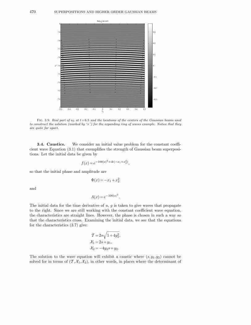
of this in Figure 3.9. While the beam centers are fairly far apart, they still providean accurate solution.

Real part of a single Gaussian beam at t=6.5

x1

x 2

−2 −1.5 −1 −0.5 0 0.5 1 1.5 27

7.2

7.4

7.6

7.8

8

Fig. 3.8. Real part of a single 3rd order Gaussian beam at t=6.5 for the expanding ring ofwaves example.


x1

x 2

Reu3 at t=6.5

−0.5 −0.4 −0.3 −0.2 −0.1 0 0.1 0.2 0.3 0.4 0.57

7.1

7.2

7.3

7.4

7.5

7.6

7.7

7.8

7.9

8

−0.3

−0.2

−0.1

0

0.1

0.2

0.3

Fig. 3.9. Real part of u3 at t=6.5 and the locations of the centers of the Gaussian beams usedto construct the solution (marked by ‘×’) for the expanding ring of waves example. Notice that theyare quite far apart.

3.4. Caustics. We consider an initial value problem for the constant coeffi-cient wave Equation (3.1) that exemplifies the strength of Gaussian beam superposi-tions. Let the initial data be given by

f(x)=e−100|x|2+ik(−x1+x22),

so that the initial phase and amplitude are

Φ(x)=−x1 +x22

and

A(x)=e−100|x|2 .

The initial data for the time derivative of u, g is taken to give waves that propagateto the right. Since we are still working with the constant coefficient wave equation,the characteristics are straight lines. However, the phase is chosen in such a way sothat the characteristics cross. Examining the initial data, we see that the equationsfor the characteristics (3.7) give:

T =2s√

1+4y22 ,

X1 =2s+y1,

X2 =−4y2s+y2.

The solution to the wave equation will exhibit a caustic where (s,y1,y2) cannot besolved for in terms of (T ,X1,X2), in other words, in places where the determinant of


the Jacobian matrix of the transformation,

∣

∣

∣

∣

∣

∣

∣

2√

1+4y22 0 8sy2√

1+4y22

2 1 0−4y2 0 1−4s

∣

∣

∣

∣

∣

∣

∣

=2√

1+4y22(1−4s)− 8sy2

√

1+4y22

(−4y2)

vanishes. Setting this expression equal to 0, we get

0=2√

1+4y22(1−4s)+

32sy22

√

1+4y22

,

0=(1+4y22)(1−4s)+16sy2

2 ,

0=1−4s+4y22 .

In space-time coordinates, (T ,X1,X2), this surface is given parametrically for p∈[1/4,∞), q∈ (−∞,∞) by

T =4p3/2,

X1 =2p+q, (3.10)

X2 =±(4p−1)3/2.

Since this is not a smooth surface, the solution to the wave equation develops a cuspcaustic (see Figure 3.10).

The equations for the various Taylor coefficients that are needed to form Gaussianbeams of first, second and third order are the same as in the previous section. Theirsuperpositions are formed as before as well.

3.4.1. Numerical calculations in the presence of caustics. Since thecharacteristics converge towards the x2 axis, the (x1,x2) support of the solution iscompressed in the x2 direction at the caustic and then it spreads apart once the rayshave passed through the caustic (see Figure 3.11). The time series shown in Figure3.11 is for a solution of the wave equation generated using a superposition of thirdorder Gaussian beams. Note that since this solution is a superposition of Gaussianbeams, it provides an accurate solution before, at and after the cusp caustic (at timet= .5). In fact, as can be seen from equations (3.10), after time t= .5 the solution iscontinuously passing through a caustic.

For the numerical calculations, a superposition of third order Gaussian beams isused to form the solution with k =104. The superposition integral (3.9) is discretizedusing a 43 by 43 grid on [−.2,.2]× [−.2,.2], and the magnitude of the solution |u| isevaluated on [−.2,1.2]× [−.2,.2] using 1401×401 grid points.

3.4.2. Order of magnitude of wave amplitude at cusp caustic. Maslovtheory predicts that the order of magnitude of the solution to the wave equation ata cusp caustic is O(k1/4) as k→∞. For a discussion of the asymptotic behavior ofthe solution, we refer the reader to [10], Chapter 6, and for a systematic classificationof several types of caustics to Chapter 7, Section 9, of [2]. To verify this behaviornumerically, we evaluate the Gaussian beam superposition at the tip of the causticfor several values of the large frequency parameter k. The superposition integral (3.9)is discretized on a parabolic grid centered about (0,0). That is, the grid points are


0

0.5

1

1.5

2

00.5

11.5

−1

−0.5

0

0.5

1

t

Cusp Caustic

x1

x 2

0 0.5 1 1.5 2−1

−0.8

−0.6

−0.4

−0.2

0

0.2

0.4

0.6

0.8

1Cusp Caustic

t

x 2

0 0.5 1 1.5−1

−0.8

−0.6

−0.4

−0.2

0

0.2

0.4

0.6

0.8

1Cusp Caustic

x1

x 2

0 0.5 1 1.5 20

0.2

0.4

0.6

0.8

1

1.2

1.4

1.6

Cusp Caustic

t

x 1

Fig. 3.10. A set of rays that form a cusp caustic. The bold line shows the caustic set that isenveloped by this particular set of rays, which are shown by the gray lines.

located on the family of curves y1 =y22 +c. For the discretization in the y2 direction,

the interval [−.2,.2] is discretized using an equispaced grid. The y1 direction is dis-cretized using the same distance between grid points as in the y2 direction with 9nodes. The exact numerical values used for the discretization are given in Table 3.3.The parabolic grid is used to minimize the calculation time, and Gaussian beams thatdon’t contribute to the solution magnitude are left out of the summation for the samereason.

A comparison between the theoretical asymptotic behavior of the magnitude ofthe solution and experimental results is shown is Figure 3.12. Note that the largerdifference at the lower frequencies does not necessarily mean that the Gaussian beamsuperposition is providing an erroneous result. The Maslov prediction is an asymptoticone, so it may not be valid at the lower frequencies.

4. Conclusion

We have shown that integral superpositions of Gaussian beams can be used to ap-proximate the initial data for PDE. Thus, through the well-posedness of the PDE, the


|u| at t=0.25

x1

x 2

−0.2 0 0.2 0.4 0.6 0.8 1−0.2

0

0.2

|u| at t=0.5

x1

x 2

−0.2 0 0.2 0.4 0.6 0.8 1−0.2

0

0.2

|u| at t=0.75

x1

x 2

−0.2 0 0.2 0.4 0.6 0.8 1−0.2

0

0.2

|u| at t=0

x1

x 2

−0.2 0 0.2 0.4 0.6 0.8 1−0.2

0

0.2

0

0.5

1

0.20.40.60.811.21.4

0

2

4

6

8

0.20.40.60.811.21.4

|u| at t=1

x1

x 2

−0.2 0 0.2 0.4 0.6 0.8 1−0.2

0

0.2

0

0.5

1

Fig. 3.11. Time series of a solution of the wave equation with localized waves passing througha cusp caustic. Solution was computed using a superposition of third order Gaussian Beams.


k y2 Nodes |u| k y2 Nodes |u|1,000 13 3.2211 375,000 253 24.35621,250 15 3.5473 500,000 291 26.30722,500 21 4.7616 625,000 325 27.91413,750 27 5.6188 750,000 357 29.29165,000 31 6.2964 875,000 385 30.50386,250 33 6.8577 1,000,000 413 31.59057,500 37 7.3406 1,250,000 461 33.48588,750 39 7.7667 2,500,000 651 40.067710,000 43 8.1484 3,750,000 797 44.463412,500 47 8.8135 5,000,000 921 47.856925,000 65 11.1066 6,250,000 1,029 50.658837,500 81 12.6194 7,500,000 1,127 53.064850,000 93 13.7773 8,750,000 1,217 55.184962,500 103 14.7272 10,000,000 1,301 57.087675,000 113 15.5388 12,500,000 1,455 60.410287,500 123 16.2510 25,000,000 2,057 71.9804100,000 131 16.8882 37,500,000 2,519 79.7282125,000 147 17.9965 50,000,000 2,907 85.7177250,000 207 21.8198

Table 3.3. Details of the discretization used to obtain the magnitude of the wave equationsolution at a cusp caustic.

103

104

105

106

107

108

100

101

102 Magnitude at Cusp Caustic

k

|u|

1.02k1/4

Fig. 3.12. Comparison of the solution magnitude at a cusp caustic with Maslov theory pre-diction. Maslov theory predicts that |u|=O(k1/4). This behavior is present in the Gaussian beamsuperposition solution.


integral superposition gives an approximate solution. In particular, we have proveda well-posedness estimate for the wave equation and used a Gaussian beam superpo-sition to approximate the solution to the 2-D wave equation for an expanding ringof waves. The Gaussian beams in this particular case stretch to fill in the gaps thatresult due to the divergence in the rays. In traditional geometric optics methods, onewould need to insert more rays to resolve the wave field in such places. Since this isnot necessary in the presented method, this example shows the power of the Gaussianbeam method.

Another advantage of the Gaussian beam method is that the obtained solution isglobal. This means that even in the presence of caustics the Gaussian beam solutionis valid, before, after and at the caustic region. As an example, we have computed theorder of magnitude of the solution at a cusp caustic as a function of the high frequencyparameter and compared it to the asymptotic behavior predicted by Maslov theory.While in geometric optics methods the solution can be extended past caustics by usinga phase correction, a computation of the solution at a caustic is not possible. Theidentification of caustics and their corrections are non-trivial in standard geometricoptics. Using Gaussian beams, one can easily compute the global wave field.

REFERENCES

[1] V. Cerveny, M. Popov and I. Psencık, Computation of wave fields in inhomogeneous media —Gaussian beam approach, Geophys. J. R. Astr. Soc., 70, 109–128, 1982.

[2] V. Guillemin and S. Sternberg, Geometric Asymptotics, Mathematical Survey and Monographs,American Mathematical Society, 14, 1977.

[3] N.R. Hill, Prestack Gaussian-beam depth migration, Geophysics, 66, 1240–1250, 2001.[4] L. Hormander, On the existence and the regularity of solutions of linear pseudo-differential

equations, L’Enseignement Mathematique, XVII, 99–163, 1971.[5] L. Klimes, Expansion of a high-frequency time-harmonic wavefield given on an initial surface

into Gaussian beams, Geophys. J.R. Astr. Soc., 79, 105–118, 1984.[6] L. Klimes, Discretization error for the superposition of Gaussian beams, Geophys. J.R. Astr.

Soc., 86, 531–551, 1986.[7] S. Leung, J. Qian and R. Burridge, Eulerian Gaussian beams for high frequency wave propa-

gation, Geophysics, 72, SM61–SM76, 2007.[8] J. Ralston, Gaussian beams and the propagation of singularities, Sudies in PDE, Stud. Math.,

23, 206–248, 1982.[9] N.M. Tanushev, J. Qian and J.V. Ralston, Mountain waves and Gaussian beams, SIAM Mul-

tiscale Modeling and Simulation, 6, 688–709, 2007.[10] M.E. Taylor, Partial Differential Equations I: Basic Theory, Appl. Math. Sci., Springer-Verlag,

115, 1996.

Date post:	11-Feb-2022
Category:	Documents
Upload:	others
View:	4 times
Download:	0 times

SUPERPOSITIONS AND HIGHER ORDER GAUSSIAN BEAMSâˆ— 1

Documents