bibbild.abo.fibibbild.abo.fi/ediss/2014/suominen_petteri.pdf · Supervised by Academy Professor...

Thermal reactions of the

major hydrocarbon components of biomass gasification gas

Petteri Suominen

Petteri Suominen | Therm

al reactions of the major hydrocarbon com

ponents of biomass gasification gas | 2014

Painosalama Oy | ISBN 978-952-12-3150-6

9 7 8 9 5 2 1 2 3 1 5 0 6

Laboratory of Industrial Chemistry and Reaction Engineering

Process Chemistry Centre

Department of Chemical Engineering

Åbo Akademi University

Turku/Åbo 2014

Thermal reactions of the major hydrocarbon components of biomass gasification gas

Petteri Suominen

Laboratory of Industrial Chemistry and Reaction Engineering Process Chemistry Centre

Department of Chemical Engineering Åbo Akademi University

Turku/Åbo 2014

Supervised by

Academy Professor Tapio Salmi Laboratory of Industrial Chemistry and Reaction Engineering Process Chemistry Centre Åbo Akademi University

Reviewers Professor Pertti Koukkari VTT Technical Research Centre of Finland Professor Juha Tanskanen Chemical Process Engineering, Faculty of Technology University of Oulu Opponent Professor Juha Tanskanen Chemical Process Engineering, Faculty of Technology University of Oulu

ISBN 978-952-12-3150-6 Painosalama Turku/Åbo 2015

iii

Rome wasn't build in a day.

- But they were laying bricks every day

Even if the dream is big and sometimes seemingly unreachable,

just do your daily work and don't lose the sight of your dream

iv

Preface

This work was done between February 2008 and December 2013 at the Laboratory of Industrial

Chemistry and Reaction Engineering, Department of Chemical Engineering at Åbo Akademi

University. The research is a part of activities of the Åbo Akademi Process Chemistry Centre (PCC), a

centre of excellence financed by Åbo Akademi University.

I would like to express my gratitude to my supervisor, Professor Tapio Salmi for his guidance which

has been irreplaceable for writing this thesis. Likewise, the help of Dr. Pekka Simell (VTT) and Dr.

Matti Reinikainen (VTT) is greatly appreciated. Also, invaluable help has been provided by Dr. Kari

Eränen with instrumentation and experimental work.

I would like to thank all my colleagues from the Laboratory of Industrial Chemistry and Reaction

Engineering. It has been a privilege and great opportunity to work with all of you. A special thank to

Dr. Teuvo Kilpiö for sharing his knowledge and thoughts about modeling.

Last but by no means least, I would like thank my family members for their patience during past years.

Thank you Hanna and my parents. And of course my aunt Leila.

The financial support of the Finnish Funding Agency for Technology and Innovation (TEKES) through

the UCGFunda project (2008-2011) is gratefully acknowledged. In addition, the financial support from

the Makarna Olins foundation (2011-2012) and Åbo Akademi University is gratefully acknowledged.

Åbo, November 2014

Petteri Suominen

v

Abstract

Gasification of biomass is an efficient method process to produce liquid fuels, heat and electricity. It is

interesting especially for the Nordic countries, where raw material for the processes is readily available.

The thermal reactions of light hydrocarbons are a major challenge for industrial applications. At

elevated temperatures, light hydrocarbons react spontaneously to form higher molecular weight

compounds. In this thesis, this phenomenon was studied by literature survey, experimental work and

modeling effort.

The literature survey revealed that the change in tar composition is likely caused by the kinetic entropy.

The role of the surface material is deemed to be an important factor in the reactivity of the system. The

experimental results were in accordance with previous publications on the subject. The novelty of the

experimental work lies in the used time interval for measurements combined with an industrially

relevant temperature interval.

The aspects which are covered in the modeling include screening of possible numerical approaches,

testing of optimization methods and kinetic modelling. No significant numerical issues were observed,

so the used calculation routines are adequate for the task. Evolutionary algorithms gave a better

performance combined with better fit than the conventional iterative methods such as Simplex and

Levenberg-Marquardt methods.

Three models were fitted on experimental data. The LLNL model was used as a reference model to

which two other models were compared. A compact model which included all the observed species

vi

was developed. The parameter estimation performed on that model gave slightly impaired fit to

experimental data than LLNL model, but the difference was barely significant.

The third tested model concentrated on the decomposition of hydrocarbons and included a theoretical

description of the formation of carbon layer on the reactor walls. The fit to experimental data was

extremely good. Based on the simulation results and literature findings, it is likely that the surface

coverage of carbonaceous deposits is a major factor in thermal reactions.

vii

Referat

Termiska reaktioner av låga kolväten med låga molekylvikter

Förgasning av biomassa erbjuder en effektiv process för produktion av bränsle, värme och elektricitet.

Speciellt användbar är processen för de nordiska länderna som är rika på råmaterial med tanke på

denna process. De termiska reaktionerna framför en stor utmaning för hela processen. Vid höga

temperaturer, kolväten med låga molekylvikter reagerar spontant och producerar tyngre molekyler. I

denna avhandling har detta fenomen studerats genom litteratursökning, experimentellt arbete samt

matematisk modellering.

Litteraturarbetet avslöjade att skillnaderna i tjärans sammanfattning beror på kinetisk entropi.

Ytmaterialet är en viktig variabel i reaktiviteten för systemet. De experimentella resultaten

överensstämmer med tidigare publicerade data. Nyheten i det experimentellt arbetet ligger i det

använda intervallet för reaktionstiderna samt industriellt relevant temperaturintervall.

De synpunkter som täcks av matematisk modellering är analys av möjliga numeriska problem, test av

olika optimeringsmetoder samt kinetisk modellering. Inga betydande numeriska onoggrannheter

observerades och de använda beräkningsrutinerna ansågs vara tillfredsställande. Evolutionära

algoritmer fungerade effektivare och gav bättre anpassning till mätdata jämfört med de konventionella

iterativa metoder så som Simplex- och Levenberg-Marquardt-metoder.

viii

Tre olika modeller anpassades till experimentella data. LLNL modellen användes som referensmodell

för de två övriga modeller. En kompakt modell som innehåller alla observerade komponenter

utvecklades. Parameterestimering visade att anpassningen till experimentell data var en aning sämre än

för LLNL -modellen men skillnaden var inte avsevärd.

Den tredje testade modellen koncentrerade sig på sönderfall av kolväten och inkluderade en teoretisk

beskrivning av formation av kolskikt på reaktorväggarna. Anpassningen till experimentella data var

ytterst bra. På basis av simuleringar och litteraturarbete, kan man konstatera högst sannolikt att ytans

täckningsgrad av kolrester är en betydande faktor i högtemperaturreaktioner.

ix

Articles & manuscripts

This thesis is a monography based on the following articles and manuscripts.

I. Thermal Reactions of the Main Hydrocarbon Components in Gasification Gas, submitted

II. Parameter Estimation of Complex Chemical Kinetics with Covariance Matrix Adaptation

Evolution Strategy, MATCH, Communications in Mathematical and in Computational Chemistry

68 (2012) No. 2, 469-476

III. A reduced reaction mechanism for light hydrocarbon thermal reactions, submitted

IV. Peak Function as a Correction Term for Radical Reaction Kinetics, submitted

V. Modeling of thermal reactions of methane-ethene-hydrogen mixture in quartz glass reactor,

submitted

Articles I-V were written and edited by the author. All the experiments, coding and modeling was

made by the author.

x

Conference presentations related to thesis

A reduced reaction mechanism for light hydrocarbon thermal reactions – oral presentation

EU COST Action CM0901 Annual Meeting 2011 Zaragoza, Spain

Parameter Estimation of Complex Chemical Kinetics with Covariance Matrix Adaptation Evolutionary

Strategy – oral presentation, Advanced Computational Methods in Engineering 2011 Liége, Belgium

xi

Other scientific work

Hydrogenation of sugars – combined heat and mass transfer

Kilpiö, T., Suominen, P., Salmi, T., Sugar hydrogenation – combined heat and mass transfer, Computer

Aided Chemical Engineering, 32 (2013), 67-72

Mass Transfer in a Porous Particle – MCMC Assisted Parameter Estimation of Dynamic Model under

Uncertainties

Suominen, P., Kilpiö, T., Salmi, T., Mass Transfer in a Porous Particle – MCMC Assisted Parameter

Estimation of Dynamic Model under Uncertainties, Computer Aided Chemical Engineering, 33 (2014),

277-82

Mass Transfer in a Porous Particle – MCMC Assisted Parameter Estimation of Dynamic Model under

Uncertainties – accepted for oral presentation

24th European Symposium on Computer Aided Process Engineering 2014 Budapest, Hungary

Hydrogenation of sugars – combined heat and mass transfer – poster presentation

23rd European Symposium on Computer Aided Process Engineering 2013 Lappeenranta, Finland

xii

Contents

Preface ......................................................................................................................................................iv Abstract ..................................................................................................................................................... v Referat ..................................................................................................................................................... vii Articles ..................................................................................................................................................... ix Conference presentations related to thesis ................................................................................................ x Other scientific work ................................................................................................................................ xi Contents .................................................................................................................................................. xii 1 Introduction ....................................................................................................................................... 1

1.1 Biomass gasification .................................................................................................................. 1 1.2 Aim and scope of this thesis ....................................................................................................... 4

2 Experimental section ......................................................................................................................... 5 2.1 Materials ..................................................................................................................................... 5 2.2 Reactor system ........................................................................................................................... 6 2.3 Analytical procedure .................................................................................................................. 7

3 Modeling aspects .............................................................................................................................. 9 3.1 Optimization approach ............................................................................................................. 10

3.1.1 Evolution algorithms in general ........................................................................................ 11 3.1.2 Evolutionary strategy with covariance matrix adaptation ................................................ 13 3.1.3 In-house stochastic optimization routine based on the PyEvolve ..................................... 13

3.2 Parameter estimation software ................................................................................................. 13 3.3 Key reactions ............................................................................................................................ 15 3.4 Entropy contributions ............................................................................................................... 17 3.5 Modified Arrhenius equation – thermodynamic explanation for challenges in modeling ....... 19 3.6 Positive and non-positive activation energies .......................................................................... 20 3.7 The models used ....................................................................................................................... 22

3.7.1 LLNL model ..................................................................................................................... 22 3.7.2 A compact model .............................................................................................................. 22 3.7.3 A surface activity corrected model ................................................................................... 31

3.8 Reactor model .......................................................................................................................... 34 4 Experimental results, modeling and discussion .............................................................................. 35

4.1 Experimental results ................................................................................................................. 35

4.2 Summary of modeling efforts .................................................................................................. 47 4.2.1 Amount of good solutions ................................................................................................. 52 4.2.2 Differential algebra ........................................................................................................... 52 4.2.3 Unconventional modelling solutions ................................................................................ 52

4.3 Discussion – gas-phase or surface reaction? ............................................................................ 55 5 Conclusions ..................................................................................................................................... 59 Notations ................................................................................................................................................. 63 References ............................................................................................................................................... 64 Appendix I .............................................................................................................................................. 68 Appendix II ............................................................................................................................................. 83 APPENDIX III ......................................................................................................................................... 135

1

1 Introduction

1.1 Biomass gasification

Gasification is a process which converts carbon-containing feedstock at high temperature to syngas.

Optimal syngas is a mixture of hydrogen and carbon monoxide with a minor amount of carbon dioxide.

The difference between combustion and gasification is in the amount oxygen. In gasification, the

amount of oxygen is very small compared to combustion.

The gasification process consists of five principal processes. Dehydration, pyrolysis, combustion,

gasification and water-gas shift reaction. During dehydration, water in the gasified material is

evaporated. The second step, pyrolysis, produces volatiles and char. After the pyrolysis, resulting char,

which can be up to 70 % lighter than the raw material, is gasified and partially burnt. The simplified

reaction mechanism for combustion is presented in Eq. 1. Carbon containing compounds (CCC) react

with oxygen to produce carbon dioxide and other oxides depending on the composition of the

feedstock. Simultaneously, char (CHAR) is gasified by steam. The reaction is given in Eq. 2. The

water-gas shift reaction presented in Eq. 3. is a reversible reaction and it alters the carbon monoxide –

hydrogen ratio of syngas depending on the process conditions. In practice, syngas contains besides the

desired components also methane and other light hydrocarbons. A reaction which produces methane is

given in Eq. 4. A subsequent reaction producing ethane is shown in Eq. 5.

CCC + O2 → CO2 + H2O (1)

CHAR + H2O → H2 + CO (2)

1

Introduction

2

CO + H2O ↔ H2 + CO2 (3)

4 CO + 2 H2O → CH4 + 3 CO2 (4)

CH4 + CH4 → C2H4 + 2 H2 (5)

Gasification as such is an old process. First industrial-scale applications are from the 19th

century as

town gas was produced either by gasification or carbonization. In 1920’s, applications to manufacture

synthetic chemicals were introduced and during World War I and II, the production of liquid fuels was

an important application of gasification. The renaissance of gasification began in 1990’s when the

awareness of the green-house effect was increased. The gasification of biomass offers an carbon-

neutral way to produce energy.

The total use of biomass for energy production is globally approximately 52 EJ/a1. This is one tenth of

the total global energy supply. Almost two thirds of this amount is consumed in developing countries

for cooking and heating. However, gasification as a process for the utilization of biomass is still quite a

minor application. Less than 5 MWth of synthesis gas is produced globally2.

Gasification of biomass is an efficient alternative for liquid fuel production via Fischer-Tropsch-

synthesis or for power and heat production. The gasification process has attended a large global

attention and is particularly important for Nordic countries which are rich in woody biomass per capita.

One of the biggest challenges in the gasification of biomass is accompanied with tar formation. This is

an obstacle specific to biomass treatment as the gasification of coal does not produce these

components. Tar formation has been studied intensively but it still remains a challenge3. Tar

components cause problems in several steps of the process, for instance, during cleaning and reforming

2

Introduction

3

processes4 by blocking the pipelines. To overcome this big problem, fundamental knowledge about the

tar formation and decomposition is needed. This implies that the reaction mechanisms and kinetic

models of the radical and catalytic reactions involved should be determined.

At elevated temperatures, hydrocarbons undergo thermal reactions, which include rearrangement

reactions, polymerizations, redistribution reactions and numerous decomposition reactions5. Even if the

amount of tar components formed during the gasification could be suppressed, the lighter

hydrocarbons, such as methane and ethene continuously react to produce tar throughout the process,

provided that the temperature is sufficiently high. Tar can block pipelines and cause catalyst

deactivation. Therefore, an accurate model of the cleaning and reforming processes must include even

thermal reactions. In order to develop a model for these steps, it is necessary to understand the various

reactions, which produce tar out of lighter hydrocarbons and to reveal how the tar components

decompose.

The thermal reactions of the two major hydrocarbons in the gasification gas, ethene6 and methane

7,8,9,

have been investigated previously. There has been published even a study on a ethene-methane mixture

but the pressures investigated were below atmospheric, the temperature range was narrower and the

residence times used in the experiments were several magnitudes larger than in this work10

.

Thermal reactions of hydrocarbons have been discussed traditionally in the context of crude oil

cracking11

. The thermal reactions are mostly considered to be reactions between radicals, but some

important reaction routes between a radical species and a molecular species12,13

have been suggested,

too. The reaction mechanisms are in general very complex.

3

Introduction

4

A particular challenge in modeling this phenomenon is the high uncertainty in published parameter

values. Several articles give uncertainties of up to an order of magnitude. This has lead to much debate

in scientific community about the accurate values of the kinetic values and in many cases modeling

efforts concentrate in fine-tuning a certain part of a large reaction mechanism.

1.2 Aim and scope of this thesis

The aim of this thesis was to investigate how the main hydrocarbon components in gasification gas

react under the conditions of gasification gas reforming. The scope of the thesis is limited to

atmospheric pressure in order to exclude the pressure from the variable list. The modeling part of the

thesis concerns parameter estimation of complex systems appearing in the gasification gas, and

discusses the reliability of the literature data of kinetic parameters.

4

Introduction

5

2 Experimental section

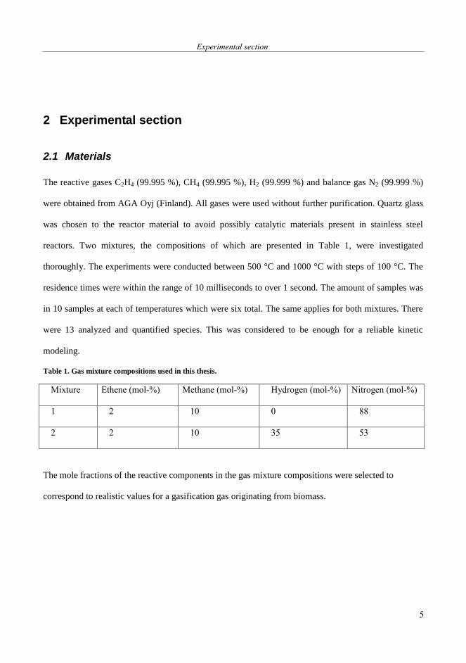
2.1 Materials

The reactive gases C2H4 (99.995 %), CH4 (99.995 %), H2 (99.999 %) and balance gas N2 (99.999 %)

were obtained from AGA Oyj (Finland). All gases were used without further purification. Quartz glass

was chosen to the reactor material to avoid possibly catalytic materials present in stainless steel

reactors. Two mixtures, the compositions of which are presented in Table 1, were investigated

thoroughly. The experiments were conducted between 500 °C and 1000 °C with steps of 100 °C. The

residence times were within the range of 10 milliseconds to over 1 second. The amount of samples was

in 10 samples at each of temperatures which were six total. The same applies for both mixtures. There

were 13 analyzed and quantified species. This was considered to be enough for a reliable kinetic

modeling.

Table 1. Gas mixture compositions used in this thesis.

Mixture Ethene (mol-%) Methane (mol-%) Hydrogen (mol-%) Nitrogen (mol-%)

1 2 10 0 88

2 2 10 35 53

The mole fractions of the reactive components in the gas mixture compositions were selected to

correspond to realistic values for a gasification gas originating from biomass.

5

Experimental section

6

2.2 Reactor system

A tubular reactor (i.d. 9 mm, length 300 mm) operating in upflow mode was placed in a tubular oven

(Carbolite Furnaces MTF 12/25A) for heating. The gas flows were controlled by mass flow controllers

(Brooks 5850). The stainless steel tubesbetween the reactor and the analyzer, gas chromatograph

(Hewlett-Packard 6890N) (GC), were heated to 170 C by electric coils to avoid condensation of high

molecular weight products. The pressure in the system was monitored on-line and kept at the

atmospheric level by withdrawing samples by a continuously running vacuum pump after the GC. This

allowed higher flow rates as only a small portion of the total flow passed the narrow GC lines. If the

whole flow would have been directed through the GC, the pressure in the system would have raised up

to 2 atm. The reactor system is illustrated in Figure 1. The experimental setup is similar to ones used in

many literature sources. None of the experimental setups in literature use a vacuum pump for sampling

which enabled higher flow rates and lower residence times than are typically used in studies of this

phenomenon.

6


7

Figure 1. Flowsheet of experimental apparatus.

2.3 Analytical procedure

The products were analyzed by an on-line GC (Hewlett-Packard 6890N) with two columns in series:

Porapak HP-Plot Q (length 30 m, i.d. 0.53 mm, film 25 μm) and HP-Mol Sieve (length 30 m, i.d. 0.53

mm, film 40 μn). Hydrogen and the lightest hydrocarbons were allowed to pass both columns but

heavier hydrocarbons passed the first column only.

The main hydrocarbons, C1-C4 alkanes, alkenes, alkynes and 1,3-butadiene were calibrated against an

internal standard. Off-line GC-MS (Agilent 6890N with Agilent 5973Network mass detector) was used

7


8

to identify the unknown compounds. The hydrocarbon concentrations were quantified by flame

ionization detector (FID) and hydrogen concentration by a thermal conductivity detector (TCD).

The calibration gas mixtures which were used in the calibration have relative uncertainties, which

influences the accuracy of the analysis results. These effects were calculated and they all were below

0.1 %. The repeatability of the analysis was checked by doing parallel measurements at randomly

selected temperatures and residence times. For each point tested the relative standard deviations were

below 1.0 %.

8


9

3 Modeling aspects

Modeling the thermal reactions of light hydrocarbons is in general a very tedious task. There are

basically two possible directions where to proceed; either large, detailed models varying from several

hundreds of reactions14,15

to over 16000 elementary reactions16

and everything in between17

or,

alternatively engineering models based on the few non-elementary reactions can be considered.

For industrial applications, models based purely on hydrocarbon reactions are not sufficient as there are

minor and trace compounds present in the gasification gas, for instance ammonia, NOx, hydrogen

sulfide, and SOx, in product mixtures which affect the product distributions. Therefore, detailed models

become even larger. They are needed to gain insight in the mechanisms of soot formation. As the

models grow larger, their applicability to practical cases which require rapid solutions, is reduced.

Engineering models have their advantages as well as their disadvantages. Their computational cost is

much lower, but they do not offer any mechanistic explanation to the physical phenomena behind the

soot formation. They are also restricted to a quite narrow operating window. New parameters must be

estimated always when the operating conditions are altered. The issue is that the new parameters might

significantly differ from the old ones which makes the parameter estimation task harder. This kind of

model has always a strongly adaptive character.

The parameter estimation, which is a numerical optimization problem, becomes more and more

challenging as the dimensionality of the system increases. This is mainly because the choice of the

initial parameter values becomes harder and harder as the amount of local minima increases in the

9

Modeling aspects

10

objective function. Another issue in the parameter estimation is presented in Figure 2. If the shape of

the minimum is highly oblong, the path which an iterative method such as a Newton or a quasi-Newton

algorithm takes may become long and the maximum allowed number of iterations is reached before the

absolute minimum is reached.

Figure 2. Badly chosen initial value for a gradient-based method.

3.1 Optimization approach

Stochastic optimization methods such as evolutionary algorithms (EA), swarm algorithms, simulated

annealing, quantum annealing and many others offer a way to overcome to some extent the previously

presented problems related to the dimensionality of the optimization problem. A recent review article

was written by L. Elliott et al.18

The main challenge in using classical Newton and quasi-Newton algorithms is the need of finding

suitable initial values for the algorithm. If suitable initial values are found, iterative methods

outperform the stochastic methods. In recent years, hybrid algorithms19

have gained popularity to

combine the advantages of the both optimization method classes.

10

Modeling aspects

11

An interesting idea was presented by L. Elliott et al.20

. In their work, they combined the parameter

estimation with the mechanism reduction scheme. The results obtained by this method in their study are

comparable to those obtained by commonly used mechanism reduction methods.

As a working hypothesis, it was assumed that a probable cause for the inaccuracies in model

predictions could be the challenges in optimization. For that reason, a state-of-art, stochastic

optimization algorithm, evolutionary strategy with covariance matrix adaptation(CMA-ES)21

was

tested in this study.

The detailed models of tar formation from light hydrocarbons are very complex, consisting of several

hundreds of reactions. As the amount of estimated parameters can be as high as three times the amount

of reactions, parameter estimation of chemical kinetics for tar formation is a practical example of an

optimization problem, for which conventional gradient/derivative based algorithms are difficult to

implement. It has been proposed that the limit above which stochastic optimization methods

outperform the gradient based methods is as low as ten dimensions.

After noticing that the problem was not in optimization, a more easily applicable stochastic

optimization routine build around the PyEvolve22

package was used.

3.1.1 Evolution algorithms in general

Evolution algorithms are effective and robust methods for optimization. Their biggest disadvantage is

the poor convergence performance and therefore they are most efficient in global optimization

11

Modeling aspects

12

problems that have many local optima. They have been used in parameter estimation of complex

chemical kinetics, but have not gained popularity over conventional gradient/derivative based methods,

which are computationally lighter in simpler parameter estimation tasks. In large parameter estimation

tasks, however, evolution algorithms have a clear advantage as the choice of initial parameter values is

by far simpler task as it is for gradient/derivative based methods.

Evolution algorithms can be divided in different techniques based on the implementation details. These

techniques include genetic algorithm, genetic programming, evolution programming, neuroevolution

and evolution strategy. For this paper, an evolution strategy (ES) was chosen for parameter estimation.

The selection process in evolution strategies is based on the fitness rankings rather than the actual

fitness values and it is deterministic. This is one of the main reasons for the robustness of ESs. Besides

selection, mutation is used as a search operator. The step-size of mutation is often governed by self-

adaptation to keep the progress in the evolution window. Another technique to ensure the convergence

to the optimum of a function is cumulative step size adaptation.

Evolution strategies have been previously used in parameter estimation of complex chemical kinetics

by Polifke et al23

. In that work, a simple (μ + λ)-ES by Rechenberg et al24

. was used. Some

improvements to this work has been proposed by Elliott el al18

. including addition of recombination

operation, which is occasionally used in evolution strategies to prevent the algorithm to stuck on local

optima. Other types of evolution algorithms, mainly genetic algorithms, and also other types of

stochastic algorithms, such as particle swarm and differential evolution (DE) have also been applied to

parameter estimation in chemical kinetics.

12

Modeling aspects

13

3.1.2 Evolutionary strategy with covariance matrix adaptation

To our work, an evolution strategy with covariance matrix adaptation (CMA-ES) by Hansen and

Ostermeier21

was chosen. Hansen and Ostermeier depict the step to CMA-ES from an ES with isotropic

mutation distribution as comparable to a step from a simple gradient-based method to a quasi-Newton

method, e.g. a step from local gradient to approximation of inverse Hessian matrix. CMA-ES has

already been applied to many real-world search problems. The advantage of CMA-ES over the

conventional ESs is the added invariance properties.

3.1.3 In-house stochastic optimization routine based on the PyEvolve

For parameter estimation of the surface corrected model, a stochastic optimization routine was

programmed. The software utilizes the PyEvolve package22

. The algorithm behind the package is not as

sophisticated as the CMA-ES but much more easier to implement in practice and actually just as

effective. The code of the our implemantion is presented in Appendix 2.

3.2 Parameter estimation software

The parameter estimation software mostly used in our laboratory, Modest25

, was soon deemed too

cumbersome to be applied in this kind of work. The reason for this is that many of the published

models are available as a Chemkin26

input file which is completely different from Modest input files.

Therefore, a new parameter estimation software was designed and programmed. The software is

presented in detail in Appendix 1. It is based on the Chemkin II software26

which was distributed as a

source code. The parameter estimation software utilized the pre-processor and Senkin modules of the

Chemkin II to simulate the reaction scheme. The CMA-ES parameter estimation software was used to

13

Modeling aspects

14

find the optimal values for kinetic parameters. The software includes also an in-house driver and post-

processor. The software is schematically presented in Figure 3.

Figure 3. A schematic view of the parameter estimation software use in this work.

The initial strategy parameters are manually inserted to CMA-ES algorithm. Likewise, the model is

written to an input file to the SENKIN module of the CHEMKIN II software package. The parameter

estimation is started and CMA-ES sends the proposed coefficients for parameters to in-house driver

program. The SENKIN module simulates the model with parameter values, which are calculated to be

the product of the proposed coefficient and literature value of the respective kinetic parameter. After a

successful simulation, the in-house driver starts the in-house post-processor, which calculates the sum

of squares of the simulated values and our experimental results. The post-processor returns this value

to driver which returns it to CMA-ES algorithm as a fitness value. At the same time, both in-house

modules record the all-time best values. CMA-ES then proposes new values for coefficients, which

14

Modeling aspects

15

undergo the same process until a termination condition is met. When a termination condition is met,

CMA-ES produces the results of its workings. The in-house driver produces a CHEMKIN input file

with best found parameter values and post-processor gives results in a form, which can easily be

plotted graphically.

3.3 Key reactions

The reaction network for this kind of system is complex. Figure 4 presents the possible reactions of

hydrogen radicals with ethyne, ethene and ethane. There are two principal reactions: abstraction and

addition. A radical species is created in both cases. The same applies for ethane and ethyne.

Figure 4. Hydrogen radical attack on ethyne, ethene and ethane.

The situation increases rapidly in complexity as illustrated in Figure 5. The number of possible

reactions is now five as the length of hydrocarbon increases by one carbon atom. If similar figures

would be drawn for even longer hydrocarbon species, the amount of reactions would increase further.

15

Modeling aspects

16

Figure 5. Hydrogen radical attack on propene.

It is worth noticing that at elevated temperatures, a variety of energetically strained radicals can exist

which additionally increases the size of the reaction system.

Obviously, the hydrocarbons do not necessarily react solely with hydrogen radicals. It is totally

possible that the opposite occurs, that is, hydrogen molecule reacts with hydrocarbon radicals, and the

hydrocarbon-hydrocarbon reactions are also possible. The only limitation is that the molecule-molecule

reactions are much slower than the molecule-radical reactions. Radical-radical reactions can also occur

but the low concentrations of the radical species make these reactions less probable.

Campbell et al27

have studied the methyl radical coupling in the presence of catalytic materials. They

concluded that at least 40 % of the ethane formed is a result of gas-phase reactions, not surface

reactions. Cho et al.28

concluded that the formation of hydrocarbon radicals cannot be solely a gas-

16

Modeling aspects

17

phase process. Grubbs and George29

have studied the effect of different reactor materials on the

hydrogen radical concentrations and their results show that there is a clear difference in the

concentrations depending on the reactor material.

It seems that even though the formation of radicals occurs in large extent on the surfaces of the reactor,

even on the catalytically inactive ones, the radicals react in gas phase. Therefore, the physical

properties of the surfaces in the reactor vessel affect strongly the product distributions. To further

complicate the issue, the carbonaceous deposits formed in the reactor have different surface properties

than the reactor materials which results in time-dependent sorption effects.

The results obtained by Kopinke et al.30

show that the formation of carbon layer depends on the reactor

material. The process on steel surface is highly erratic. Some unsteady behavior can be observed also

on quartz surfaces but the experimental data show that the process proceeds in S-curve like fashion.

The erratic characteristics of the carbon layer formation on steel surfaces is an unfortunate effect in

modeling industrial applications. Fortunately, the surface area-to-volume ratio31

in industrial

applications is such that the importance of the surface reactions is likely to be less than in a laboratory

scale.

3.4 Entropy contributions

In an ab initio study, Li and Brenner32

calculated rate constants and analyzed the enthalpy and entropy

effects on them. Based on quantum chemical calculations, they concluded that at temperatures relevant

to this study, the entropy is an important variable when considering the product distributions. The

17

Modeling aspects

18

translational entropy increases the probability of the β-scission reaction, which is illustrated in Figure

6, compared to the addition of a hydrogen atom to an unsaturated hydrocarbon. These calculations are

in accordance with experimental results of Rye33

and Balooch and Olander34

. Similar results were also

obtained by Frenklach35

by numerical simulations.

Figure 6. Beta-scission reaction.

Rotational entropy favors hydrogen abstraction reactions. Perhaps the most notable consequence of the

entropy considerations is how the β-scission is favored over the hydrogen addition reaction at higher

temperatures. This was experimentally observed by Rye33

and similar results were obtained by Li and

Brenner32

by quantum chemical calculations. Without taking the entropy effects into account, addition

reactions would dominate over β-scission even at high temperatures. Interestingly, the tar formed in

lower temperatures is aliphatic but aromatic tar is formed at higher temperatures. The results obtained

by Spence and Vahrman36

show that over 10 % of dry tar can consist of paraffins and olefins. There is

no literature about significant amounts of aliphatic compounds present in tars from high-temperature

gasification processes.

Surface chemical studies would be highly interesting in estimating the role of entropy in the tar

formation. A possible explanation to different kinds of tar produced in different temperatures is the

reduction of rotational and translational entropy for molecules in an interaction with a surface. This

would cause different products for pure gas-phase systems as well as catalyzed, Eley-Rideal and

Langmuir-Hinshelwood types of reaction systems. Studying this would require experimental work to

18

Modeling aspects

19

determine at which temperatures surface reactions are possible on pure quartz and on carbonaceous

deposits.

3.5 Modified Arrhenius equation – thermodynamic explanation for challenges in modeling

An interesting aspect in modelling the chemistry related to combustion and gasification processes is a

modified Arrhenius equation presented in Eq. 6. The resemblence to an expression used in transition

state theory (TST), which is shown in Eq. 7, is apparent.

TR

En

ref

a

T

TAk

exp

(6)

TR

H

R

S

bcc

h

Tkk

,,

expexp (7)

Based on the literature findings presented in previous chapter, it is clear that the entropy contributes to

the product distributions of the thermal reactions. This leads intuitively to think that the exponential

temperature dependency in modified Arrhenius equation in this application, actually depicts the

entropy contribution of the reaction. If this thought is developed further, a probable cause for deviation

of the predictions by detailed reaction mechanisms can be worked out. There are namely problems

with applying transition theory to high temperature radical reactions.

First, the transition theory assumes that all the intermediate species can reach a Bolzmann distribution

of energies. That is, the intermediate species are enough stable and therefore being enough long-lived.

If this is not a case, then the momentum of reaction trajectory from reactants to intermediates can be

19

Modeling aspects

20

transferred to products, which affects the product distributions. As many of the hydrocarbon radical

species are short-lived, there is a good chance that the product distributions differ from the theoretical

ones even though the kinetic constants would be correctly defined for every elementary reaction in

mechanism.

Second, the transition state theory fails if the atomic nuclei do not behave according classic mechanics.

In quantum mechanics, for every barrier with finite amount of energy exists a possibility that a particle

can tunnel across. Many of the activation energies are low in radical species reactions. Therefore,

probability for tunneling increases and again, the product distributions may differ from the ones

predicted by classical kinetics.

Third, according to transition state theory the reactions proceed through the lowest energy saddle point

at potential energy surface. This is the case for reactions at low temperatures but at high temperatures,

higher energy vibrational modes are populated. This leads to more complex behavior of the molecules

and ultimately to transition states which are far away from the energetic minimum. And even this

phenomenon increases the deviation from the predicted product distributions.

3.6 Positive and non-positive activation energies

Conventionally, the activation energy of a reaction is considered to be equivalent to the energy barrier

between two minima of the potential energy. The value of activation energy is positive for both exo-

and endothermic reactions. In some cases the activation energy can be non-positive. The theoretical

background for this phenomenon has been published by Houk and Rondan37

and Mozurkewich and

20

Modeling aspects

21

Benson38

. The background is most easily presented by the Tolman interpretation of the activation

energy39

presented in Eq. 8.

Eact = <E>TS - <E>R (8)

The activation energy (Eact) is a difference of the average energies of the transition state (<E>TS) and

reactants (<E>R). Three cases are possible.

In the first case, the transition state is a tight one. Some of the degrees of freedom are transformed to

vibrational modes as the reactants are transformed to the transition state. Generally, this has a very

minor effect on the average internal energy by the decrease in the kinetic energy and the increase in the

potential energy by the breaking and forming of the bonds is much larger. In this case, which is also the

most common one, the activation energy is positive.

The second alternative is that the transition state is loose. Neither the changes in the potential energy or

the kinetic energy are significant and the activation energy is very close to zero.

A negative activation energy is the consequence of the third alternative. This can happen if the reaction

which is assumed to be elementary is not truly elementary but proceeds via a stable intermediate. In

this case, the types of the transition states between the reactants and the intermediate, and the

intermediate and the products together with the magnitudes of their energy thresholds dictate the sign

of the activation energy.

21

Modeling aspects

22

3.7 The models used

3.7.1 LLNL model

The LLNL model40

is a classical detailed reaction mechanism for gas-phase reactions of light

hydrocarbons. It includes 687 reversible reactions and has been validated for n-butane, propane,

ethyne, ethane and methane. It was chosen to be the standard model to which the other tested models

were compared.

3.7.2 A compact model

In many literature sources, it is stated that some of the kinetic parameters for detailed mechanisms of

gasification and combustion are not estimable at all or only in order of magnitude. The assumption was

made that a reduction of the dimensionality of the model would result in easier parameter estimation

tasks. Therefore, a compact model which includes all the observed species, was designed. The reaction

mechanism consists of 37 reversible reactions and 30 species. This model is presented in Table 2.

Table 2. Rate constant parameters after the parameter estimation. Units are cm, mole, cal, K and Pa. Reference is

for the publication from which the reaction has been taken.

reaction A n Ea Ref

1 32524242 HCHCHCHC 4.72E14 0.00 7.13E4

41

2 352442 CHHCCHHC 1.41E9 0.00 1.00E3

14

22

Modeling aspects

23

3 HHH 2 6.55E4 0.00 1.02E5 41

4 HHCHHC 52242 1.03E13 0.00 6.82E4

41

5 HCHCH 34 6.26E20 0.00 1.02E5

41

6 HHCHCHC 644232 4.98E11 0.00 7.31E3

41

7 23242 HHCHHC 7.00E13 0.00 2.87E3 41

8 62325242 HCHCHCHC 1.38E13 0.00 2.19E4 41

9 HHCHHC 62252 2.56E12 0.00 1.30E4

41

10 1045252 HCHCHC 1.07E13 0.00 0 41

11 945242 HCHCHC 2.83E11 0.00 8.06E3

41

12 HHCHC 8494 9.71E13 0.00 3.84E4

42

13 63539422 HCHCHCHC 7.22E11 0.00 9.00E3 43

14 36394 CHHCHC 1.97E13 0.00 3.00E4

14

15 73342 HCCHHC 3.34E11 0.00 7.71E3

14

16 22833273 HCHCHCHC 1.22E12 0.00 0 44

17 HHCCHCH 5233 1.05E13 0.00 1.07E4

45

23

Modeling aspects

24

18 HHCHC 2232 7.74E16 0.00 3.61E4

41

19 22232 HHCHHC 9.73E13 0.00 0 41

20 23242 HHCHHC 2.99E14 0.00 1.54E4 41

21 234 HCHHCH 1.84E14 0.00 1.25E4 41

22 422323 CHHCHCCH 3.92E11 0.00 0 41

23 25363 HHCHHC 3.14E13 0.00 5.63E3 46

24 22242 HMHCMHC 4.00E15 0.00 9.03E4 41

25 25464 HHCHHC 3.40E12 0.00 6.00E4 47

26 33354 CHHCHHC 9.81E13 0.00 0

14

27 HHCHCHC 563333 2.96E12 0.00 0

48

28 HHCHC 2333 4.96E12 0.00 7.84E4

14

29 562333 HCHCHC 4.93E13 0.00 0

14

30 87356 HCCHHC 3.95E12 0.00 0 14

31 62555364 HCHCHCHC 9.74E12 0.00 2.26E4 14

32 HHCHHC 66256 3.95E12 0.00 7.89E3

14

24

Modeling aspects

25

33 HHCHCHC 682256 3.95E12 0.00 1.01E4

41

34 25868 HHCHHC 2.51E14 0.00 1.60E4 41

35 7102258 HCHCHC 4.09E13 0.00 1.01E4

41

36 HHCHHC 8102710 1.02E14 0.00 7.89E3

41

37 HHHCHCHC 8105555 9.83E10 0.00 8.00E3

41

The presented reaction mechanism is based on the literature survey. Main source of reaction and kinetic

data is the kinetic database of National Institute of Standards and Technology (NIST). The species in

the model were chosen based on our experimental work. After the selection of the species, some well-

known reactions were chosen as a backbone of the model. Then several combinations of different

published reactions were tested and the combination which gave the best fit to experimental data was

chosen. During the whole process of selecting reactions, the different stages of chain reaction were

considered, so that the necessary branching was obtained.

The goal of the modelling was to keep to the number of reactions to the minimum, with reasonable

accuracy, so that the model could be implemented to engineering environment tools where

computational effort is required to other calculations as well. The model was also limited to gas-phase

reactions at the moment. Different surface reactions are of even greater interest than the gas-phase

reactions but the analysis of such reactions would require a new experimental setup.

25

Modeling aspects

26

The mechanism is initiated by the reactions 1-5 forming the hydrogen, methyl, vinyl and ethyl radicals.

The first molecular product formed is 1,3-butadiene by the Reaction 6. Also C2-species, ethyne and

ethane are formed in the early phase of the reaction scheme. There are several reactions leading to these

species. They are needed to obtain the necessary form of the chain reaction with enough branching

reactions compared to inhibiting ones. Combination reactions between C2-species form the C4-species

and C3-species are formed mainly from the rearrangement reaction between C2-species and C4-species

or by decomposition reactions of C4-species, although one reaction, number 15, between a C2-species

and methyl leads to formation of propyl radical.

1,3-butadiene is an important intermediate to the formation tar and soot precursors. Consecutive

reactions with hydrogen radicals form a propargyl and propadienylidene radicals which form phenyl

radical by the Reactions 30 and 32. Another route to cyclic compounds which was chosen to model

proceeds also via 1,3-butadiene. Together with allyl radical it forms cyclopentadienyl which can react

to other cyclic and polycyclic compounds. Ethyne is an important species for the growth of the

aromatic compounds and the consecutive addition of ethyne to phenyl yields naphthalene according to

Reactions 33-36. Naphthalene is also the heaviest compound in our model.

Hydrogen radicals are the driving force in the chain reaction. They are formed in 14 different reactions

and consumed in 8 reactions. This explains also the importance of the form of the reaction mechanism.

The mechanism needs to be constructed so that the formation rate of hydrogen radicals is equivalent to

the formation rate of hydrogen radicals in the reactor. In a way, this may seem obvious but in

constructing a reduced reaction mechanism which depicts the formation of tar and soot from the lighter

hydrocarbons, it is not necessary to model every reaction and species. Some of the reactions and

26

Modeling aspects

27

species have very little or even no effect on the outcome of the model. These can be identified by

mathematically analysing the equation system.

3.7.2.1 Sensitivity analysis of the reduced reaction mechanism

The sensitivity analysis was performed by SENKIN part of the Chemkin 2 software package. The

results of these analyses were used to identify the most dominant parameters in the system. The

sensitivity coefficients were calculated to the reactants: hydrogen, methane and ethene. Besides these,

benzene was investigated by sensitivity analysis. This is unfortunately only a theoretical investigation

as no experimental data is available for benzene. Benzene is among the unwanted species and therefore

interesting compound for the sensitivity analysis. A positive coefficient indicates that the reaction

enhances the species production and a negative one is a sign of opposite effect.

3.7.2.1.1 Methane

In the presence of hydrogen, methane at 1000 °C was sensitive to three reactions. Its production was

enhanced by the Reactions 27 and 30. The Reaction 33 competes with the Reaction 30 and therefore

methane production was negatively influenced by it. At 900 °C, the same reactions were important but

two new important reactions appeared. Reaction 22 consumes methane and Reaction 24 forms

methane. At 800 °C, methane is no longer sensitive towards Reactions 24 and 33. As temperature is

lowered to 700 °C and 600 °C, only Reaction 27 remains influential on the methane concentration. At

500 °C, methane is not sensitive to any of the reactions. This according to literature findings which

propose that methane works as a radical transfer species. Our experimental work does also support this

as methane is neither formed nor consumed at lower temperatures. It seems that methane does have a

27

Modeling aspects

28

minor role in the formation aromatic compounds but otherwise it only affects the overall reactivity of

the system.

In comparison, if the mixture did not contain hydrogen methane sensitivity was considerably lower at

lower temperatures. On contrary, high temperatures exhibit a different behaviour. Methane sensitivity

is higher if no initial hydrogen is present in the mixture. The probable cause is the formation of

hydrogen from the methane by direct decomposition which is reported to happen at temperatures above

875 °C. At high temperatures, aromatic compounds are forming and as with previous mixture, methane

is slightly affected by the Reactions 27, 30, 33, 34 and 37 at 900 °C and 1000 °C. Likewise, at 800 °C

is still high enough temperature for the formation of aromatic compounds and methane was sensitive to

Reactions 30, 33 and 34. Reactions 30 and 34 lower the methane concentration and Reactions 37, 33

and 27 increase it. At 700 °C, there is a clear difference to hydrogen containing mixture. Methane was

sensitive to Reactions 30 and 33 instead of 27 and interestingly Reaction 30 affects negatively the

concentration of methane rather than positively as it was the case in the hydrogen containing mixture.

This depends most likely on the fact there is very little hydrogen in the system competing for the

methyl radicals as the formation of hydrogen begins at temperatures over 700 degrees in hydrogen free

mixtures. At 600 and 500 °C methane was even more passive than in the presence of hydrogen.

3.7.2.1.2 Hydrogen

Initially hydrogen free mixture produces hydrogen at elevated temperatures. The sensitivity analysis of

this mixture at 1000 degrees shows that many reactions affect the system. Reactions 18, 24, 27, 33 and

37 enhance the consumption of hydrogen and Reactions 22, 30 and 34 produce hydrogen. Termination

Reactions 22 and 30 cause the increase in hydrogen production as the amount free radicals in the

28

Modeling aspects

29

system diminishes and this increases the probability hydrogen radicals abstract hydrogen from

molecular species. The Reaction 27 increases the concentration of phenyl radicals which then react

with hydrogen and Reaction 24 produces precursor to this pathway. At 900 °C Reaction 21 is also

sensitive for the hydrogen concentration and produces hydrogen. At 800 °C, same reactions were

detected. Difference is that Reactions 18, 33 and 37 have a positive effect on the hydrogen

concentration whereas Reaction 22 starts consuming hydrogen. At temperature below 800 °C, only

traces of hydrogen were observed in the experiments. This does not though affect the sensitivity

analyses. Same reactions are sensitive as a new reaction, Reaction 15 becomes relevant. This indicates

that the radical transfer properties of methane are important. As temperature is lowered by another 100

°C to 600 °C, same reactions are still important, but also Reaction 25 becomes important. This would

indicate that 1,3-butadiene plays some role also in the formation of aliphatic tar and not just in the

formation of aromatic tar and soot compounds. At the lowest temperature in our work, the amount of

relevant reactions increases. This suggests that hydrogen has an important role in the formation

aliphatic tar compounds.

There were plenty of important reactions in the initially hydrogen free mixture but the case is different

for hydrogen containing mixture. At 1000 °C and 900 °C only 3 reactions are sensitive. These are

numbers 27 and 30 which consume hydrogen and number 33 which forms hydrogen. At 800 °C two

more hydrogen consuming reactions are found, numbers 21 and 22. This is caused most likely by the

radical transfer properties of methane. At 700 °C Reaction 33 produces hydrogen and Reactions 15, 20

and 22 consume it. At 600 °C and 500 °C only hydrogen consuming reactions were of some

importance, namely 20 and 22.

29

Modeling aspects

30

3.7.2.1.3 Ethene

Ethene has the highest conversions of the initial compounds. At 1000 °C without initial hydrogen its

consumption is enhanced by the Reactions 33 and 37 and production is enhanced by the Reactions 30

and 34. At 900 °C the same reactions are enhancing the production but there are more reaction

affecting the consumption, namely Reactions 18, 21, 22, 24, 25, 33 and 37. One hundred degrees lower,

at 800 °C still the same reactions are responsible for the enhancement of production rate but the

consuming reactions alter again. This time the Reactions 21, 27, 33 and 37 were analysed. Even in the

context of ethene reactivity, the transfer from aromatic products to aliphatic products can be observed

in the sensitivity analysis. At 700 °C, Reactions 30 and 34 are enhancing the production of ethylene but

amount of important consuming reactions diminishes and only Reaction 33 was identified by the

sensitivity analysis. At even lower temperatures, there are no clearly influential reactions.

Comparison to hydrogen containing mixture it is interesting that as was the case with methane, the

reactions effects can be inverted between the two mixtures. At 1000 °C, both Reaction 30 and 33 have

opposite effects compared to hydrogen-free mixture. Reaction 33 enhances the formation and

Reactions 24, 27 and 30 do the opposite. This is actually the opposite to the behaviour of methane. At

900 °C the situation is basically the same, only the numerical values are slightly lower and also

Reaction 22 is important. At 800 °C only consuming reactions were found. These are Reactions 15, 20,

21, 22, 24, 25, 27, 30 and 33. 700 °C is similar, there is one more consuming reaction, Reaction 19, and

the values are lower. At 600 °C, Reactions 15, 20, 21, 22, 27, 33 and 34 enhance the consumption of

ethene. At 500 °C, the consuming reactions are 20, 22, 27 and 34.

30

Modeling aspects

31

3.7.2.1.4 Benzene

Benzene is one of the unwanted products of the thermal reactions. At 1000 °C, the strongest favouring

effect on the formation comes from the Reactions 7 and 27. This corresponds to pathway via 1,3-

butadiene. The strongest opposite effect comes from the Reactions 3 and 33. Reaction 33 is not wanted

as it leads to heavier aromatic compounds. Reaction 3 is also the strongest inhibiting reaction at 900

°C. The strongest formation favouring Reactions are 1 and 33. At 800 °C, strongest formation favoring

Reactions are 1, 2, and 33. The strongest reactions in favouring the consumption are 6 and 9. At 700 °C

and below, it becomes harder and harder to find reactions which would favour the consumption of

benzene. Other side is that the production rate of benzene becomes practically zero.

Results from the hydrogen containing mixture are quite similar at 1000 °C differing only slightly in

magnitude. At 900 °C and below it is not possible to find reactions which would favour the

consumption of benzene. It seems that hydrogen plays an important role in the formation of tar and

soot.

3.7.3 A surface activity corrected model

The reaction mechanism presented in Eq 9-15 was fitted to experimental data49

. As proposed by Cho et

al 50

, even though the reactions mostly occur in gas-phase, the formation of radical species takes largely

place on the surfaces of the reactor walls. Therefore, the mechanism includes a component for

carbonaceous deposit (CD) on the reactor wall. The surface properties of quartz glass and the formed

carboneous deposits are different and assumptions was made that carbon coating is more active in

forming hydrocarbon radicals. Another assumption is that the formation of the layer occurs so that the

growth of an existing deposit is more likely than a formation of a new nucleiting centre. This

assumption is in accordance with the visual inspection of the reactor as after experiments with short

31

Modeling aspects

32

residence times, the reactor walls were covered with spots of deposits. With longer residence times,

these spots grow in area.

The mechanism consists of six irreversible reactions and a sigmoidal growth curve for carbonaceous

deposits (CD).

PSEUDOCDCH 4 (9)

PSEUDOHCHC 4242 (10)

PSEUDOCDHC 42 (11)

PRODUCTSCDPSEUDO (12)

4CHCDPSEUDO (13)

42HCCDPSEUDO (14)

221

0

1

)( A

e

AAtCD

dx

xt

(15)

The idea behind the surface activity corrected model is that the formation of carbonaceous deposit on

the reactor walls has a different proficiency to form hydrocarbon radicals than the clean quartz glass

surface. The activity is assumed to increase in a fashion of a sigmoidal curve. This assumption was

made based on visual inspections made occasionally on the reactor after an experiment. If the residence

time was short, there were only tiny black spots spread around the reactor walls. With prolonged

residence times, the spots grew covered more and more of the surface.

32

Modeling aspects

33

The purpose of this model is to answer the question whether the reactor surfaces affect the outcome of

gas-phase reaction scheme. That is why the model concentrates on the decomposition of methane and

ethene.

The mechanism consists of five components: methane (CH4), ethene (C2H4), pseudo intermediate

(PSEUDO), stable products (PRODUCTS) and carbonaceous deposits (CD). Other components besides

CD are stoichiometric but to depict a sigmoidal curve with elementary kinetics would have required

several more reactions and therefore a Bolztmann curve was chosen to model the growth of the carbon

layer on the reactor surface.

The Bolztmann curve is a sigmoidal curve which has four parameters. A1 and A2 are the initial and

final value. Two other parameters, x0 and dx correspond to point of inflection and time constant. For

the parameter A2, unity was chosen for value. The parameter values for A1, x0 and dx were estimated.

The Bolztmann curve was chosen over other sigmoidal curves because of its combination of simplicity

and easy adjustability.

Many sources suggest that a molecule-molecule reaction between two ethene molecules is a typical

initiation reaction for thermal reactions of major hydrocarbon components in biomass gasification gas.

Therefore, it was chosen as an initiation reaction to mechanism. But a mechanism consisting only of

molecule-molecule reactions is unrealistic and five reactions, one for each hydrocarbon component

and three for pseudo intermediate was taken into mechanism. These reactions represent molecule-

radical reactions.

33

Modeling aspects

34

This approach is limited to mixtures containing large amounts of hydrogen. Based on the work of Li

and Brenner32

it was supposed that mainly hydrogen radicals affect reactivity.

3.8 Reactor model

Two reactor models were used in this study. The common thing for both is that the reactor is a tube

reactor with plug flow. The plug flow conditions were confirmed by calculating the Reynolds number

for the lowest used flows. In the first one, a temperature profile for the lower half of the reactor was

measured. A pocket inside the reactor for the thermocouple does not allow measurements for the upper

part of the reactor and therefore it was assumed that the temperature profile in the reactor was

symmetric for the lower and the upper part of the reactor. The second model was an isothermal one.

This type of model which takes into account only the isothermal part of the reactor is occasionally used

in modeling thermal reactions. In a modern oven, the non-isothermal part is rather short compared to

the iso-thermal one and it is assumed that it has a minor effect on the product distributions.

34

Modeling aspects

35

4 Experimental results, modeling and discussion

4.1 Experimental results

The experiments at the temperature interval of 500-1000ºC follow the pattern previously described by

Zhil’tsova et al51

. There is a short induction period followed by a phase of an exponential growth. The

exponential growth then decelerates to a more slowly reacting phase, either a growing or decreasing

one, depending on the species. Eventually, a steady-state operation is reached. Our experimental results

follow the three first phases but a steady-state operation was not reached in all temperatures. The

concentration profiles of individual components for the two mixtures are presented in Figures 7-18.

The chosen components are: hydrogen, methane, ethyne, ethene, ethane and 1,3-butadiene.

35

Experimental results, modeling and discussion

36

Figure 7. Hydrogen concentrations for mixture 1 as function of residence time.

Figure 8. Hydrogen concentrations for mixture 2 as function of residence time.

36


37

Figure 9. Methane concentrations for mixture 1 as function of residence time.

Figure 10. Methane concentrations for mixture 2 as function of residence time.

37


38

Figure 11. Ethane concentrations for mixture 1 as function of residence time.

Figure 12 Ethane concentrations for mixture 2 as function of residence time

38


39

Figure 13. Ethene concentrations for mixture 1 as function of residence time.

Figure 14. Ethene concentrations for mixture 2 as function of residence time.

39


40

Figure 15. Ethyne concentrations for mixture 1 as function of residence time.

Figure 16. Ethyne concentrations for mixture 2 as function of residence time.

40


41

Figure 17. 1,3-butadiene concentrations for mixture 1 as function of residence time.

Figure 18. 1,3-butadiene concentrations for mixture 2 as function of residence time.

41


42

From Figures 7-8, the following observations can be made: in the experiments with hydrogen

containing mixtures, the yield of hydrogen is more or less constant, while hydrogen is starting to form

at 700 °C in the experiments without initial hydrogen in the initial mixture. This supports the reported

behavior of the tar formation. Between 700 and 800 °C, there is a shift from the aliphatic tar to the

aromatic one and therefore it can be expected that hydrogen is formed.

At 700 °C, the steady-state is obtained at approximately 900 ms and the yield of hydrogen exceeds

slightly 0.1 mol-%. At 800 °C, these values are 900 ms and 1 mol-%. As the temperature is raised to

900 °C, the figures become 600 ms and 3 mol-%. At our highest temperature 1000 °C, the steady-state

is obtained even faster, in 400 ms and the yield of hydrogen is 10 mol-%.

The hydrogen concentration profiles for the mixture without initial hydrogen show that the hydrogen

starts to form from the hydrocarbons somewhere within the interval 700-800 C. This is also the same

interval where the tar composition turns from aliphatic waxes to aromatic compounds. This

phenomenon was not observed in the mixture with initial hydrogen. Therefore, in practical

applications, the formation of hydrogen cannot be used as an indication of the formation of aromatic

species.

As a result of the large excess of hydrogen in mixture 2, more ethane is formed compared to mixture

1. This would indicate that ethene as presented in Figures 13-14, and at higher temperatures even

acetylene are hydrogenated to ethane. At higher temperatures, ethane concentrations are significantly

lower than those of acetylene. This is expected as acetylene is the most thermally stable C2-species.

42


43

Below 800 °C, ethene behaves quite similarly for both mixtures. The hydrogen needed to convert

ethene to ethane is formed mainly from methane if it is not present in the mixture initially. Above 800

°C, the ethane formation is reduced if no initial hydrogen is present.

Acetylene is formed at temperatures exceeding 700 °C. It seems that acetylene has an important role

in the formation of aromatic tar compounds.

An interesting observation from the methane concentration profiles showns in Figures 9-10 is that

hydrogen stabilizes methane. Unfortunately, this effect is only temporary and after a certain delay,

similar concentrations are obtained. This is likely to be caused by a direct decomposition to elements.

This phenomenon is becomes visible at 875 °C52

. However, at higher temperatures the decomposition

curves have very similar topologies, indicating that even relatively small amounts of hydrogen are

sufficient to have an impact on the hydrocarbon reactivities.

The yields of ethane in Figures 11-12 show a different behavior from hydrogen. In the hydrogen-

containing mixture, the yields have a maximum at 600 °C. The amounts change from 500 °C to 1000

°C as follows: 0.2, 0.8, 0.5, 0.2, 0.15, and 0.15 mol-%. The respective times to obtain these yields are

1000, 900, 400, 100, 100, and 100 ms. It is worth noticing that at temperatures 900 °C and 1000 °C,

ethane has a maximum yield at approximately 100 ms, after which the yields start to decrease. In non-

hydrogen mixtures, the behavior is different from the hydrogen containing mixtures. The times needed

to obtain the steady-state or the maximum yields are higher up to 800 °C. The values listed in the same

order as previously: not observed, 1000, 900, 400, 100, and 100 ms. The maximum yields are

practically similar in the investigated temperature interval, namely 0.01 mol-%.

43


44

Figures 15-16 show how acetylene was formed at 700 °C and 800 °C faster in the hydrogen

containing mixture. The maximum yields were approximately the same, 0.015 mol-% and 0.15 mol-%

respectively. At 900 °C and 1000 °C, the acetylene formation took place faster and the maximal yields

were higher, 0.5 mol-% and 1.0 mol-%, respectively.

C3-species are also important intermediate products in the tar formation process. Interestingly,

propene was never observed in significant amounts. Contrary to ethane, propane is formed only in

hydrogen-free mixtures. Therefore, the hydrogenation of unsaturated C3-species does not occur in

significant amounts. This is especially interesting as the lighter C2-species are readily hydrogenated. A

possible explanation for this behavior could be that propyne is resonance-stabilized with two isomers,

propyne and propadiene. Propyne and propene are formed at temperatures over 700 °C, as there is no

initial hydrogen present in the system and at temperatures exceeding 900 °C for the hydrogen-

containing mixtures. Propene is likely to be consumed in dimerization reactions, too.

The product distributions of these dimerization reactions are expectedly influenced by the

temperature profile of the reactor. Allylic hydrogen is more reactive than vinylic hydrogen and

therefore leading to non-conjugated C6-species especially at low temperatures. These species can

relatively easily undergo rearrangement and cyclization reactions to mono-unsaturated cyclic

compounds, which were observed in small quantities by off-line GC-MS. At higher temperatures even

vinylic hydrogen is likely to be radicalized forming higher molecular-weight compounds with

conjugated double bonds. For instance, a reaction between two propene molecules with vinylic radicals

can react to 2,4-hexadiene.

44


45

At high temperatures, propene is formed and consumed rapidly most likely indicating the formation

of heavier hydrocarbons; for instance, formation of cyclopentadiene according to reaction 6. However,

at lower temperatures, a steady-state of the propene yield is obtained. As propene is formed only in

hydrogen-free mixtures at lower temperatures, this could be interpreted as an indication of balanced

dimerization reactions and corresponding decomposition reactions.

Besides 1,3-butadiene in Figures 17-18, C4-species were observed in few occasions. At 500 °C, n-

butane was detected in small amounts, indicating the formation of aliphatic tar. On the contrary, at 900

and 1000 °C, minor amounts of butenes and butanes were formed. 1,3-butadiene, on the other hand,

was observed at each temperature and mixture. As reaction 3 shows, this compound is formed easily

from the ethene which is abundantly converted to other hydrocarbons. Therefore, it seems that this

compound is one of the most important intermediate products in the formation both aliphatic and

aromatic tars.

Many of the compounds found in the product mixture are known from previous works done on the

pyrolysis of ethene 6,53

. However, the product distributions obtained in this study differ vastly from the

values reported previously. According to Back et al6., propene, ethane and 1- butene are the main

products of ethene pyrolysis at 500 °C. Practically no propene was observed in our experiments and

1,3-butadiene was one of the main components instead. Compared to Norinaga et al14

., the biggest

difference is the low amounts of the C3-species in their work carried out at 900 °C. This can be

explained, if the proposed decomposition reaction to ethenyl and methyl radicals is considered

reversible and therefore balanced by the concentration of methyl radicals. The major reason for the lack

of 1-butene in our experiments is probably the shorter residence times compared to those used by

Bossard and Back10

.They proposed that 1-butene is formed mainly by decomposition reactions and

45


46

these decomposition reactions are favored by low pressures54

. Though methane conversions are low

compared to ethylene conversions, it seems that even minute amounts methane-derived radicals affect

the thermal chemistry of hydrocarbons.

The amount of carbon deposited in the reactor is higher than for the gasification gas when

considering the mixture without hydrogen. When hydrogen is added to the reacting mixture, the

amounts of tar compounds in the reactor correspond more accurately to those of real gasification gas.

This is in accordance with hydrogen content inhibiting carbon deposition as proposed previously by

Becker et al55

.

Considering the thermal stability of the hydrocarbons, it is easy to notice that most of the light

molecular weight compounds are intermediates. The huge difference in magnitude of the ethyne and

1,3-butadiene concentrations in two mixtures, indicate that hydrogen has a major role in the reactivity

of these compounds.

Perhaps the most striking feature of the experimental data is the clear peak in the profiles before 0.5

seconds. At first, this was thought to be caused by mistakes in the experimental work but the

phenomenon is too consistent to be caused by an inadequate laboratory practice. There are probably

few experimental points which are caused by larger experimental scattering but in large scale, the

probable reason is the growth of carbonaceous deposits on the quartz surface. The exact mechanism is

unknown but the curvature of the profiles suggests that the mechanism resembles the Kisliuk

mechanism56

, i.e, the growth of existing deposits is more probable than the formation of new centra of

growth.

46


47

4.2 Summary of modeling efforts

A purely homogeneous gas-phase reaction model is not suitable for a quantitative description of the

system. Even the tested detailed model had difficulties in predicting the behavior of the system

correctly.

A hypothesis was that this problem could be solved by parameter estimation. The uncertainties of the

published kinetic parameter values57

are high. The uncertainties range from 30 % up to a factor of 10.

As Figures 19-20 demonstrate, this is not the case, even though a better fit to experimental data was

obtained but still better results were needed. A CMA-ES algorithm21

along with other schemes was

tested and even though the evolutionary algorithms gave a better fit to the experimental data than

iterative methods, probably due to the high dimensionality of the problem, the accuracy of the

predictions remained inadequate.

47


48

Figure 19 Our compact model at 1000°C

Figure 20 LLNL model at 1000°C

48


49

Similar results were obtained by estimating the parameters of the LLNL model40

and our compact

model. The simulation results by the LLNL have a slightly better accuracy than our compact model but

the difference is not large. It is worth noticing that the LLNL with its approximately 600 reactions is

much smaller than the detailed models which comprise of over ten thousand reactions.

Comparing the predictions of LLNL n-butane flame model and our model, it can be noticed that their

predictions on the major species are very similar. The only observable difference is the fact that LLNL

model performs better when the residence time exceeds approximately 1 s. This is due to fact that

LLNL model includes the formation of carbonaceous deposits, whereas our model is limited to gas-

phase reactions only. This indicates that the gas-phase pre-equilibrium is reached in approximately 1 s,

but the formation of condensed phase continues to grow slowly.

Figures 19-20 show that, both the LLNL and the developed reduced, reaction mechanism are able to

describe the behaviour of the system quantitatively. The developed model performs well with short

residence times. At longer residence times, the lack of depositing carbon affects the model predictions

slightly negatively. To compare the goodness of the fit for the developed model regression analysis was

performed in Excel by data analysis tool pack. The R2 value of the model was 0.823 prior to the

parameter estimation and 0.966 after the parameter estimation. The calculated sum of least square

values was over 10 % lower for the parameter estimated model.

The major source of error in model are the minor compounds, such as ethyne and 1,3-butadiene, which

are expected to participate in the formation of tar and soot. Therefore, a model which is limited to gas-

49


50

phase reactions, cannot predict these compounds accurately. Another possible source of error, a minor

one compared to the previous one, is the analysis of hydrogen. Hydrogen is analysed by a temperature

conductivity detector, which does not have the same detection limits as the flame ion detector gives for

the analysis of hydrocarbons.

The goodness of the fit was estimated by the sum of squares, which was calculated from experimental

results of our own. Kinetic experiments were conducted at six temperatures from 500 °C to 1000 °C

and for two different compositions. Both mixtures contained 2 mol-% ethene and 10 mol-% methane

and the other one had 35 mol-% of hydrogen. Nitrogen was used as a balance gas. All in all, 120

experimental points were recorded for the calculation of sum of squares. The experimental setup is

presented in detail in Suominen et al49

. In case of a detailed kinetic model from LLNL, the sum of

squares was lower, even though the magnitude was the same as with our reduced kinetic model prior to

the parameter estimation.

A regression analysis of the model predictions and the experimental values was performed by the data

analysis toolpack in Excel. It was observed that the R2-value, the coefficient of determination,

increased significantly by the parameter estimation and was 0.966 after the parameter estimation. The

R2-value is a measure of how likely the model predicts the future outcomes. The sum of square values

in both cases were over 10 % lower after the parameter estimation compared to prior the parameter

estimation. Graphical illustrations of the experimental values compared to model predictions prior to

and after parameter estimation are presented in Figure 19-20.

In case of the LLNL model, the advantage of the adaptation of the mutation distribution could not be

observed as the parameter values were not allowed to change more than 5 % and the best combination

50


51

of parameter values was found at less than 30n function evaluations which is according to Hansen and

Ostermeier21

the limit for the adaptation to improve the strategy behaviour. In the case of our reduced

model, more evaluations were required to obtain a solution with an acceptable accuracy. Therefore, the

adaptation did have time to evolve. The same restriction of 5 % was applied even here. Even in this

case, the full advantage of the adaptation as the limit of 100n2 function evaluations was not reached.

During the development of our model, we tried to perform the parameter estimation on preliminary

models, too. In a case when the estimated parameters were not close to the literature findings,

considerably more function evaluations were needed to reach a satisfactory accuracy for the model. In

attempts like these, no restrictions were applied. This indicates that CMA-ES could be an interesting

candidate for parameter estimation in such applications, where the magnitudes of the parameters are

unknown and the amount of parameters is large. Possible applications are problems, in which diffusion

and/or adsorption effects are added to complex chemical kinetics.

Hansen and Kern58

have reported that increasing the population, in many cases, considerably increases

the performance of the algorithm. In our applications, this kind of behaviour could not be observed in

significant magnitude. As some test functions in their report did not either exhibit such behaviour, this

cannot considered a surprising result. It is, though, possible that the population size should have been

increased even more than we did to obtain an increase in algorithm performance.

Different parameter estimation approaches were tested. We tried to estimate all the parameters in the

modified Arrhenius equation presented in Eq. 6 and different combinations of them. The most efficient

way was to estimate only one parameter. Intuitively, this is clear as the size of covariance matrix

increases but the amount of data from which it is estimated does not increase.

51


52

4.2.1 Amount of good solutions

The difficulties in the parameter estimation lead to a hypothesis that there are many possible reaction

mechanisms which give a good fit to experimental data. This assumption was tested by Markov Chain

Monte Carlo (MCMC) assisted parameter estimation technique, where all possible reactions were given

two parameters: a numeric rate constant and a Boolean parameter which either includes or excludes the

reaction from the model. The purpose was to test whether the MCMC could converge to a right

mechanism and to determine the amount of mechanisms which yield a good fit to experimental data. In

the scheme, a mechanism of eight species was used. The pseudo experimental data consisted of

simulation results at eight time points. The scheme was not able to the converge to right solution and

the amount of solutions with good fit to experimental data was estimated to be approximately 2.5 %.

4.2.2 Differential algebra

Differential algebra was tested to study the parameter estimability of the system. A similar approach as

suggested in G. Margaria et al.59

, N. Meshkat et al.60

and M. P. Saccomani et al.61

was tested but even

the compact model was too large that the Rosenfeld-Groebner algorithm could have utilized. This is a

definitely interesting approach to evaluate the parameter estimability in the future but the extremely

high computational cost is too high for applications such as ours for the time being.

4.2.3 Unconventional modelling solutions

If a sigmoidal function such as a Boltzmann function, which is given in Equation 16, was used to

model the growth of the deposits, the fit on experimental data is excellent. Similar results can be

52


53

obtained by a peak function correction to radical concentrations as suggested by Suominen and Salmi62

.

The sigmoidal function is presented below in Figure 21.

221

1

A

e

AAty

dx

xt o

(16)

Figure 21 An example of Boltzmann function

Basically, the success behind this function is that even the clean quartz glass creates radicals, in much

slower rate than the carbenous deposits, though. By adjusting parameter A1, the initial level can be

53


54

altered. Parameter dx affects the velocity by which the deposits grow and parameter A2 gives the upper

limit, in this case, the evident choice is unity which corresponds logically to the situation where the

whole quartz surface is covered by carbenous deposits. Finally, the parameter x0 affects the placement

of the point of inflection, e.g. the point where the second derivative changes the sign.

Figure 22 concentration profiles at 700 °C; methane dashed line, ethylene dot-dashed line

54


55

The modeling results fit very well the experimental data as Figure 22 demonstrates. For methane and

ethene, the fit is excellent. The swag at the lower temperatures is caused by the formation of the

carbenous deposits on the reactor walls. The side product of this process is methane. The lower the

temperature, the later the swag appears on the methane concentration profile. At temperatures high

enough, the concentration profile of methane is flat indicating that the formation of carboneous

deposits is so fast that our experimental setup cannot observe it.

Figure 23 presents the same experimental results without the correction. If the concentration profiles

corrected for surface activity are compared to simulations of the same system without the CD effect, it

is clear that the surface coverage of carbonaceous deposits is an important variable in the system

studied. Modeling the delay without the sigmoidal curve would require a much more complex

mechanism than ours.

4.3 Discussion – gas-phase or surface reaction?

The experimental data are in accordance with the previous studies on thermal reactions of light

hydrocarbons. The reactivity of the mixture increases with temperature and more unsaturated

compunds are formed at elevated temperatures

The HACA-mechanism63,64,65

, hydrogen abstraction – C2H2 addition, is a classical theory for modelling

the growth of aromatic species. There are several cases where the HACA-mechanism fails to explain

the growth of aromatic molecules. Perhaps the main reason is that the HACA-mechanism is a slow

mechanism66,67

. Other proposed, more rapid, mechanisms include the PAC-mechanism, phenyl

addition/cyclization, and MAC-mechanism, methyl addition/cyclization, ring-ring condensation, aryl-

55


56

aryl combination, particle filler model and condensation of an aromatic radical to a neutral species. A

comparative study of the mechanisms was written by Shukla and Koshi.68

It is outside the scope for this thesis to analyze the soot formation in detail, but it is important that

components which are a part of these mechanisms are observed in this study. These compounds include

hydrogen, methane, ethyne and indirectly 1,3-butene as an intermediate to six-membered ring

structures and ethane which is a stable product at lower temperatures. These compounds are chosen to

be discussed in more detail.

A similar computational chemistry approach as Li and Brenner32

performed for ethyne, ethene, ethane

and methane would be interesting to be applied for three and four carbon atom molecules. In this way,

a better understanding for the possibilities of controlling the soot formation could be obtained.

The carbenous deposits on the reactor surface affect the system to a great extent. Even though they can

be used to control the amount of tar formed, they also affect the conversion of light hydrocarbons if the

reactor material has different surface properties than the carbonaceous deposits.

To which extent the reactions occur in the gas phase is an important and interesting question for which

our experimental apparatus could not produce necessary data. The literature concerning this issue is

controversial. If the change in tar composition from aliphatic to aromatic compounds is taught to be

caused by the kinetic entropy, then the proportion of high molecular weight aliphatic compounds to

aromatic compounds could be used to estimate the relation of gas-phase and surface reactions. As the

kinetic entropy is severely reduced during sorption, the reactions should be directed towards the

56


57

aliphatic compounds even at elevated temperatures. Therefore, it seems that gas-phase reactions are

the dominant ones at least at elevated temperatures.

The importance of the surfaces in forming radical ions is not as contradictory as the gas-phase versus

surface reaction issue. A significant amount of radicals are formed on the surface. The formed

carbenous deposits have different physical properties than the quartz glass used as the reactor material

and the concentration profiles of the product mixture exhibit a behaviour which can be explained by a

sigmoidal type of growth of the surface coverage by the carbonaceous deposits. An interesting question

remains: to which extent the surface material affects the formation of radicals and how important is the

specific surface area? Unfortunately we were unable to isolate enough carboneus deposits from the

reactor to be able to measure its surface area. Nor were we able to make any measurements considering

the possible time-dependent behaviour of the carbonaceous deposits.

Another problem related to the reactor material exists. This challenge is illustrated by Kopinke et al.30

Their measurements of deposits reveal that the mass of deposits in a steel reactor does not follow

neither a linear nor an exponential growth. The same phenomenon was observed even in their

measurements of deposits in quartz glass reactor but a distinct growth pattern can still be observed.

This is an unfortunate effect when considering the modelling of soot formation in industrial scale

equipment. Fortunately, the surface area-volume ratio31

for industrially applied reactors is more

advantageous and the overall effect is likely to be less than in laboratory scale.

Figure 23 illustrates different reaction types. Reaction A is an Eley-Rideal type of reaction where one

reactant is in the gas-phase while the other one is adsorbed on the surface. Reaction B illustrates a

Langmuir-Hinshelwood type of reaction. The difference to the reaction A is that both reactants are

57


58

adsorbed on the surface. In reaction C, a radical species is formed as a molecular species comes in

contact with a surface. Finally, reaction D depicts a situation where a molecule forms radical species in

the gas-phase. The letter M is used to mark an atom or molecule to which the reacting species collides.

Figure 23. Different reaction types: A) Eley-Rideal B) Langmuir Hinshelwood C) Radical formation on surface D)

Radical formation in gas-phase.

58


59

5 Conclusions

Description of the thermal decomposition kinetics of ethene-methane mixtures in the presence and

absence of hydrogen was investigated by literature survey, kinetic experiments and modeling effort.

Even though, the scope of the thesis was limited to the reactions of light hydrocarbon components

present in gasification gas in the presence and absence of hydrogen, the system is very complicated.

The work on this thesis is illustrated in Figure 24. The work began from design of the experimental

apparatus and planning of the kinetic experiments. Simultaneously with experimental work, first model

was developed. The kinetic data was analyzed and need for better software to handle the huge model

and large number of experimental data was recognized. With new software, a full kinetic model

approach was tested. Then the efforts were concentrated on simplifying the model. By careful

interpretation of findings from literature survey, a compact model with physical background was

developed.

59

Conclusions

60

Figure 24. A flowsheet of the thesis work

The experimental work was carried out at a temperature interval of 500-1000 ºC. This temperature

interval includes the transition temperature in product distributions from aliphatic tar to aromatic tar.

The experimental data were obtained on a time interval seldomly used. There exist shock tube

experiments from micro- to millisecond scale and there are experimental data from few hundred

milliseconds up to several seconds but data from the intermediate area from 10-20 millisecond to few

hundred milliseconds are scarce. All the experiments were carried out under atmospheric pressure.

From industrial point of view, it would be interesting to obtain measurements from elevated pressures,

60

Conclusions

61

but the modeling effort would become more difficult, if the pressure would have to be taken as an

additional parameter.

The experimental results showed a similar behavior which is depicted by Zhil’tsova et al51

. There is a

short induction period followed by an exponential growth of product molecules, after which the system

reaches a steady state

A parameter estimation software based on the Chemkin simulation software was developed. The

estimation of parameters was performed by a CMA-ES algorithm. Even other algorithms were tested

but the results were either comparable or inferior to the results obtained by CMA-ES. It is though

necessary to remember that the full power of CMA-ES was not utilized as the algorithm converged to a

result before the covariance matrix update scheme was initiated.

The Markov Chain Monte Carlo (MCMC) simulations on a simple reaction system showed that finding

a correct reaction mechanism is a tedious task, if it is based solely on experimental data. It has been

discussed that a viable method to reduce the amount of mechanisms which yield good fit to

experimental data is in-situ measurement of radical species. Unfortunately, we did not have a such an

analytical apparatus at our disposal.

Reliable numerical data on kinetic parameters would be invaluable in modeling efforts. At the current

moment, published kinetic data must be reviewed critically. Typically, uncertainties for reaction rate

parameters are from 30 % to a factor of 10 for this kind of systems. Some published models are based

on the estimating simultaneously tens of parameters. The results of this kind of approach should be

avoided.

61

Conclusions

62

The kinetic entropy seems to be among the reasons why the tar consists of aliphatic compounds at

lower temperatures but more and more aromatic compounds are produced by thermal reactions at

higher temperatures. This is affected by the reactor material and geometry.

The conversion of the light hydrocarbons to tar is affected by the forming carbonaceous deposits. The

quartz glass reactor used in our experiments has a lower surface area than the carbonaceous deposits,

and therefore, the amount of radicals formed at the surface is increased which leads to higher

conversions of light hydrocarbons.

62

Conclusions

63

Notation

A pre-exponential parameter in Arrhenius equation

b exponential parameter in Arrhenius equation

CMA-ES covariance matrix adaptation evolutionary strategy

Ea activation energy

EA evolutionary algorithm

MCMC Markov Chain Monte Carlo

63

Notation

64

References

1 E. Vakkilainen, K. Kuparinen, J. Heinimö, Large Industrial Users of Energy Biomass, IEA

Bioenergy, Task 40: Sustainable International Bioenergy Trade, 2013, Lappeenranta, Finland 2 C. Higman, State of the Gasification Industry – the Updated Worldwide Gasification Database,

Gasification Technologies Conference, Colorado Springs, US, 2013 3 L.P.L.M. Rabou, R.W.R. Zwart, B.J. Vreugdenhil, l. Bos, Tar in biomass Producer Gas, the Energy

research Centre of The Netherlands (ECN) Experience: An Enduring Challenge, Energy Fuels 23,

6189-6198, (2009) 4 P. Cahill, M. Nieminen, M. Dutton, G. Rasmussen, K. Kangasmaa, The influence of tars on hot gas

filter performance in air blown gasification of coal and biomass, in: E. Schmidt, P. Gäng, T. Pilz, A.

Dittler (Eds.), High Temperature Gas Cleaning, Institut für Mechanise Verfahrenstechnik und

Mechanik, Karlsruhe, Germany, 1996, pp. 782-793 5 S.W. Benson, G.R. Haugen, Mechanisms for some high-temperature gas-phase reactions of ethylene,

acetylene, and butadiene, J. Phys. Chem., 71, 1735-1746, (1967) 6 M.H. Back, R. Martin, The thermal reactions of ethylene in the presence and absence of small

quantities of oxygen, Int. J. Chem. Kin. 11, 757-774, (1979) 7 C.J. Chen, M.H. Back, R.A. Back, The thermal decomposition of methane. I. Kinetics of the primary

decomposition of methane and its pressure dependence, Can. J. Chem. 53, 3580-3590, (1975) 8 C.J. Chen, M.H. Back, R.A. Back, The thermal decomposition of methane. II. Secondary reactions,

autocatalysis, and carbon formation: non-Arrhenius nehavior of methyl radical with ethane, Can. J.

Chem. 54, 3175-3184, (1976) 9 C.J. Chen, M.H. Back, R.A. Back, The thermal decomposition of methane. III. Methyl radical

exchange in methane-methane-d4 mixtures, Can. J. Chem. 55, 1624-1628, (1977) 10

A.R. Bossard, M.H. Back, The homogenous thermal conversion of methane to higher hydrocarbons

in the presence of ethylene, Can. J. Chem. 68, 1401-1407, (1990) 11

B.S. Greensfelder, H.H. Voge, G.M. Good, Catalytic and thermal cracking of pure hydrocarbons –

Mechanisms of reaction, Ind. Eng. Chem. 41, 2573-2584, (1949) 12

D. Wang, A. Violi, Radical-molecule reactions for aromatic growth: A case study for

cyclopentadienyl and acenaphtylene, J. Org. Chem. 71, 8365-8371, (2006) 13

D. Wang, A. Violi, D.H. Kim, J.A. Mulholland, Formation of naphtalene, indene, and benzene from

cyclopentadiene pyrolysis: A DFT study, J. Phys. Chem. 110, 4719-4725, (2006) 14

K. Norinaga, O. Deutschmann, Detailed kinetic modeling of gas-phase reactions in the chemical

vapor deposition of carbon from light hydrocarbons, Ind. Eng. Chem. 46 3547-3557, (2007) 15

K.Norinaga, V.N. Janardhanan, O. Deutschmann, Detailed chemical kinetic modeling of pyrolysis of

ethylene, acetylene, and propylene at 1073-1373 K with a plug-flow reactor model, Int J Chem Kinet,

40, 199-208 (2008) 16

E. Ranzi, A. Frassoldati, R. Grana, A. Cuoci, T. Faravelli, A.P. Kelley, C.K. Law, Hierarchical and

comparative kinetic modeling of laminar flame speeds of hydrocarbon and oxygenated fuels, Progress

in Energy and Combustion Science, 38 (4), pp. 468-501 (2012) 17

H. Richter, S. Granata, W.H. Green, J.B. Howard: Detailed modeling of PAH and soot formation in a

laminar premixed benzen/oxygen/argon low-pressure flame, Proc. Comb. Inst. 30, 1397-1405 (2005)

64

References

65

18

L. Elliott, D.B. Ingham, A.G. Kyne, N.S. Mera, M. Pourkashanian, C.W. Wilson, Genetic algorithms

for optimisation of chemical kinetics reaction mechanisms, Prog. Energy and Combust Sci. 30, 297-

328, (2004) 19

V. Kelner, F. Capitanescu, O. Léonard, L. Wehenkel, A hybrid optimization technique coupling an

evolutionary and local search algorithm, J. Comput. Appl. Math., 215, 448-456, (2008) 20

L. Elliott, D.B. Ingham, A.G. Kyne, N.S. Mera, M. Pourkashanian, C.W. Wilson, Reaction

mechanism reduction and optimization using genetic algorithms, Ind. Eng. Chem. Res. 44, 658-667,

(2005) 21

N. Hansen, A Ostermeier, Completely derandomized self-adaptation in evolution strategies.

Evolutionary Computation, 9, 159–195 (2001) 22

C. S. Perone, Pyevolve: a Python open-source framework for genetic algorithms, ACM

SIGEVOlution, 4, 12-20, (2009) 23

W. Polifke, W. Geng, and K. Döbbeling. Optimization of Rate Coefficients for Simplified Reaction

Mechanisms with Genetic Algorithms. Combustion and Flame, 113, 119-135, (1998) 24

I. Rechenberg. Evolutionsstrategie ’94. Frommann-Holzboog, Stuttgart-Bad Cannstadt (1994). 25

H. Haario, ModEst 6.0 User Manual, Helsinki, (2010) 26

A. Lutz. SENKIN, A Fortran program for predicting homogeneous gas phase kinetics with

sensitivity analysis. Report 87-8248, Sandia National Laboratories. 27

K.D. Campbell, E. Morales, J.H. Lunsford, Gas-phase coupling of methyl radicals during the

catalytic partial oxidation of methane, J. Am. Chem. Soc. 109, 7900-7901, (1987) 28

Y. Cho, K. Choi, Y. Kim, S. Lee, Kinetic investigation of oxidative methane pyrolysis at high

CH4/O2 ratio in a quartz flow microreactor below 1073 K, Bull. Korean Chem. Soc. 29, 1609-1612,

(2008) 29

R.K. Grubbs, S.M. George, Attenuation of hydrogen radicals traveling under flowing gas conditions

through tubes of different materials, J. Vac. Sci. Technol. 24, 486-496, (2006) 30

F.D. Kopinke, G. Zimmerman, S. Nowak, On the mechanism of coke formation in steam cracking –

conclusions from results obtained by tracer experiments, Carbon, 26, 117-124, (1988) 31

W.A. Bone, J.B. Gardner, Comparative Studies of the Slow Combustion of Methane, Methyl

Alcohol, Formaldehyde, and Formic Acid, Proc. R. Soc. London A, 154, 297, (1936) 32

Y. Li, D.W. Brenner, Ab initio study of the role of entropy in the kinetics of acetylene production in

filament-assisted diamond growth environments, J. Phys. Chem. A, 110, 132-140, (2006) 33

R.R. Rye, Reaction of thermal atomic hydrogen with carbon, Surf. Sci., 69, 653, (1977) 34

M. Balooch, D.R. Olander, Reactions of modulated molecular beams with pyrolytic graphite. III.

Hydrogen, J. Chem. Phys. 63, 4772, (1975) 35

M.- Frenklach, The role of hydrogen in vapor deposition of diamond, J. Appl. Phys. 65, 5142, (1989) 36

J.A Spence, M. Vahrman, Aliphatic hydrocarbons in a low-temperature tar, J. Appl. Chem. 17, 143-

146, (1967) 37

K.N. Houk, N. G. Rondan, Origin of negative activation energies and entropy control of halocabrene

cycloadditions and related fast reactions, J. Am. Chem. Soc., 106, 4293-4294, (1984) 38

M. Mozurkewich, S.W. Benson, Negative Activation Energies and Curved Arrhenius Plots. 1.

Theory of Reactions over Potential Wells, J. Phys. Chem. 88, 6429-6435, (1984) 39

R.D. Levine, R.B. Bernstein, Molecular Reaction Dynamics, Oxford University Press, New York,

USA (1974)

65

References

66

40

N. Marinov, W. Pitz, C. Westbrook, A. Vincitore, M. Castaldi, S. Senkan. Aromatic and Polycyclic

Aromatic Hydrocarbon Formation in a Laminar Premixed n-butane Flame. Combustion and Flame,

114,192-213, (1998) 41

Tsang, W, Hampson, RF. Chemical kinetic data base for combustion chemistry. Part 1. Methane and

related compounds. J. Phys. Chem. Ref. Data,15, (1986) 42

Curran, HJ, Rate constant estimation for C-1 to C-4 alkyl and alkoxy radical decomposition. Int. J.

Chem. Kinet. 2006;38;250-75. 43

Tsang W, Chemical kinetic data base for combustion chemistry. Part 4. Isobutane, J. Phys. Chem.

Ref. Data. 1990;19;1-68. 44

Tsang W, Chemical kinetic data base for combustion chemistry. Part 3. Propane, J. Phys. Chem. Ref.

Data. 1988;17. 45

Stewart, P.H., Larson, C.W., Golden, D.M., Pressure and temperature dependence of reactions

proceeding via bound complex. 2. Application to 2CH3->C2H5+H. Combust. Flame, 1989;75;25-31 46

Tsang W. Chemical kinetic data base for combustion chemistry. Part 5. Propene, J. Phys. Chem. Ref.

Data. 1991;17; 221-73. 47

Dean, AM. Predictions of pressure and temperature effects upon radical addition and recombination

reactions. J. Phys. Chem. 1985:89:4600-8 48

Burcat, A, Dvinyaninov, M. Detailed kinetics of cyclopentadiene decomposition studied in a shock

tube. Int. J. Chem. Kinet. 1997;29; 505 – 14 49

Suominen P.; Kangas M.; Eränen K.; Reinikainen M.; Simell P.; Salmi T. Thermal Reactions of the

Major Hydrocarbon Components of the Gasification Gas at the Interval 500 – 1000 Degrees Celsius,

submitted 50

Cho Y.; Choi K.; Kim Y.; Lee S. Kinetic investigation of oxidative methane pyrolysis at high

CH4/O2 ratio in a quartz flow microreactor below 1073 K, Bull. Korean Chem. Soc. 2008, 29, 1609-

1612 51

I.V. Zhil’tsova, I.S. Zaslonko, Yu.K. Karasevich, H.Gg. Wagner, Nonisothermal effects in the

process of soot formation in ethylene pyrolysis behind shock waves, Kin. Cat. 41, 76-89, (2000) 52

R.H. Crabtree, Aspects of methane chemistry, Chem. Rev. 95 (1995) 987-1007 53

K. Norinaga, O. Deutschmann, K. J. Hüttinger, Analysis of gas phase compounds in chemical vapor

deposition of carbon from light hydrocarbons, Carbon 44, 1790-1800, (2006) 54

A. Kossiakoff, F. O. Rice, Thermal decomposition of hydrocarbons, resonance stabilization and

isomerization of free radicals, J. Am. Chem. Soc. 59 (1943) 590-595 55

A. Becker, Z. Hu, K. J. Hüttinger, A hydrogen inhibition model of carbon from light hydrocarbons,

Fuel 79 (2000) 1573-1580 56

P. Kisliuk, The sticking probabilities of gases chemisorbed on the surface of solids, J- Phys. Chem.

Solids, 1957, 95-101 (1957) 57

W. Tsang, R.F. Hampson, Chemical kinetic data base for combustion chemistry. Part I. Methane and

related compounds, J. Phys. Chem. Ref. Data, 15, 1087, (1986) 58

N. Hansen, and S. Kern. Evaluating the CMA Evolution Strategy on Multimodal Test Functions.

Parallel Problem Solving, Springer-Verlag (2004) 59

G. Margaria, E. Riccomango, M.J. Chappell, H.P. Wynn, Differential algebra methods for the study

of the structural identifiability of rational function state-space models in the biosciences, Math.

Biosciences, 174, 1-26, (2001)

66

References

67

60

N. Meshkat, M. Eisenberg, J.J. DiStefano III, An algortihm for finding globally identifiable

parameter combinations of nonlinear ODE models using Gröbner Bases, Math. Biosciences, 222, 61-

72, (2009) 61

M.P. Saccomani, S. Audoly, G. Bellu, L. D’Angiò, Examples of testing global identifiability of

biological and biomedical models with the DAISY software, Computers in Biology and Medicine, 40,

402-407, (2010) 62

P. Suominen, T. Salmi, Peak Function as a Correction Term for Radical Reaction Kinetics, submitted 63

M. Frenklach, H. Wang, Proc. Combust. Inst. 23, 1559, (1991) 64

M. Frenklach, D.W. Clary, W.C. Gardiner, S.E. Stein, Proc. Combust. Inst., 20, 887, (1985) 65

H. Wang, M. Frenklach, Combust. Flame, 110, 173-221, (1997) 66

H. Bockhorn, F. Fetting, H.W. Wenz, Ber. Bunsen-Ges. Phys. Chem. 87, 1067, (1983) 67

H. Böhm, H. Jander, D. Tanke, Proc. Combust. Inst. 27, 1605-1612, (1998) 68

B. Shukla, M. Koshi, Comparative study on the growth mechanisms of PAHs, Combustion and

Flame, 158, 369-375, (2011)

67

References

68

Appendix I

The LLNL mechanism used in the work as a Chemkin input file:

! reference:

! Marinov, N. M., Pitz, W. J., Westbrook, C. K., Vincitore, A. M.,

! Castaldi, M. J., Senkan, S. M. "Aromatic and Polycyclic Aromatic

! Hydrocarbon Formation in a Laminar Premixed n-Butane Flame"

! Combustion and Flame 114 192-213 (1998).

! UCRL-WEB-204236

! Review and release date: May 19, 2004.

!

! Date: Tue, 19 Jan 1999 11:38:35 -0800 (PST)

! From: "Nick M. Marinov" <[email protected]>

elements h o c ar n end

species

h2 h

ch4 ch3 ch2 ch ch2o hco co2 co o2 o oh ho2 h2o2 h2o

c2h hcco c2h2 c2h3 c2h4 c2h5 c2h6 ch2oh ch3o hccoh h2ccch

c3h2 ch2(s) ch2co c4h2 c5h2 c5h3 c6h2 c2 c2o c hcoh

ch2chcch hcchcch h2cccch c6h5 c6h6 c6h5o

ch2chchch ch2chcch2

h2c4o ch2chchch2 ch3oh ch2hco

c-c5h5 c-c5h5o c-c5h6 c6h5oh c10h8 c-c5h4oh c-c5h4o

c4h10 pc4h9 sc4h9 c4h8-1 c4h8-2 c4h7

c3h6 ac3h5 pc3h5

sc3h5 ch2chcho pc3h4 ac3h4 ch3co c6h5ch2 c6h5ch3

ch2chco ch3chco ch3hco chocho

c3h8 ic3h7 nc3h7 ch3chcch2 ch3ccch2

c6h5c2h5 c10h10 c10h9 c10h7

c6h4c2h3 c6h4c2h c6h5c2h3 c6h5c2h c10h7o

c6h5cho c6h5co hoc6h4ch3 c6h5ch2oh oc6h4o

oc6h4ch3 c10h7ch2 c10h7ch3

ch3c6h4ch3 indene indenyl acenphthln phnthrn

ch3chcch ch3ch2cch ch3c6h4ch2

phnthryl-1 phnthryl-9 flrnthn

ch3c6h4c2h3 ch3c6h4c2h5

c-2*4c6h6o c-c5h7 l-c5h8 l-c5h7

c10h7c2h5 c10h7c2h3 c10h7oh c6h5cco

c6h5chch c6h5cch2 c10h7cch2 c10h7cch c10h6cch

anthracn ch3indene ch3indenyl ch3phnthrn pyrene

fluoryl fluorene h2cccch2 chchcho hcccho hccco

hc4-p(def)pthn hc4-p(def)pthyl phnthroxy-1 phnthroxy-9

bz(a)ndene bz(a)ndnyl phnthrol-1 phnthrol-9 biphenyl bz(a)phnthrn

bz(ghi)fln fulvene ch3cy24pd ch3cy24pd1 ch3dcy24pd cyc6h7

fulvenyl ar n2 end

thermo

end

reactions

oh+h2=h+h2o 2.14E+08 1.52 3449.0 !Marinov 1995a

o+oh=o2+h 2.02E+14 -0.4 0.0 !Marinov 1995a

o+h2=oh+h 5.06E+04 2.67 6290.0 !Marinov 1995a

h+o2(+m)=ho2(+m) 4.52E+13 0.0 0.0 !Marinov 1995a

68

Appendix I

69

low / 1.05E+19 -1.257 0.0 / !Marinov 1995a

! h2o/0.0/ h2/0.0/ ch4/10.0/ co2/3.8/ co/1.9/

h2o/0.0/ h2/0.0/ n2/0.0/ ch4/10.0/ co2/3.8/ co/1.9/

h+o2(+n2)=ho2(+n2) 4.52E+13 0.0 0.0 !Marinov 1995a

low / 2.03E+20 -1.59 0.0 / !Marinov 1995a

h+o2(+h2)=ho2(+h2) 4.52E+13 0.0 0.0 !Marinov 1995a

low / 1.52E+19 -1.133 0.0 / !Marinov 1995a

h+o2(+h2o)=ho2(+h2o) 4.52E+13 0.0 0.0 !Marinov 1995a

low / 2.10E+23 -2.437 0.0 / !Marinov 1995a

oh+ho2=h2o+o2 2.13E+28 -4.827 3500.0 !Hippler 1995

dup

oh+ho2=h2o+o2 9.10E+14 0.0 10964.0 !Hippler 1995

dup

h+ho2=oh+oh 1.50E+14 0.0 1000.0 !Marinov 1995a

h+ho2=h2+o2 8.45E+11 0.65 1241.0 !Marinov 1995a

h+ho2=o+h2o 3.01E+13 0.0 1721.0 !Marinov 1995a

o+ho2=o2+oh 3.25E+13 0.0 0.0 !Marinov 1995a

oh+oh=o+h2o 3.57E+04 2.4 -2112.0 !Marinov 1995a

h+h+m=h2+m 1.00E+18 -1.0 0.0 !Marinov 1995a

h2o/0.0/ h2/0.0/

h+h+h2=h2+h2 9.20E+16 -0.6 0.0 !Marinov 1995a

h+h+h2o=h2+h2o 6.00E+19 -1.25 0.0 !Marinov 1995a

h+oh+m=h2o+m 2.21E+22 -2.0 0.0 !Marinov 1995a

h2o/6.4/

h+o+m=oh+m 4.71E+18 -1.0 0.0 !Marinov 1995a

h2o/6.4/

o+o+m=o2+m 1.89E+13 0.0 -1788.0 !Marinov 1995a

ho2+ho2=h2o2+o2 4.20E+14 0.0 11982.0 !Marinov 1995a

dup

ho2+ho2=h2o2+o2 1.30E+11 0.0 -1629.0 !Marinov 1995a

dup

oh+oh(+m)=h2o2(+m) 1.24E+14 -0.37 0.0 !Marinov 1995a

low / 3.04E+30 -4.63 2049.0 / !Marinov 1995a

troe / 0.470 100.0 2000.0 1.0E+15/

h2o2+h=ho2+h2 1.98E+06 2.0 2435.0 !Marinov 1995a

h2o2+h=oh+h2o 3.07E+13 0.0 4217.0 !Marinov 1995a

h2o2+o=oh+ho2 9.55E+06 2.0 3970.0 !Marinov 1995a

h2o2+oh=h2o+ho2 2.40E+00 4.042 -2162.0 !Marinov 1995a

ch3+ch3(+m)=c2h6(+m) 9.22E+16 -1.174 636.0 !Walter 1990

low / 1.14E+36 -5.246 1705.0/ !Walter 1990

troe/ 0.405 1120.0 69.6 1.0E+15/

h2o/5.0/ h2/2.0/ co2/3.0/ co/2.0/

ch3+h(+m)=ch4(+m) 2.14E+15 -0.4 0.0 !Tsang 1986

low/ 3.31E+30 -4.0 2108.0 / ! (a)

troe / 0.0 1.0E-15 1.0E-15 40.0/

h2o/5.0/ h2/2.0/ co2/3.0/ co/2.0/

ch4+h=ch3+h2 2.20E+04 3.0 8750.0 !Miller 1992

ch4+oh=ch3+h2o 4.19E+06 2.0 2547.0 !Marinov 1995

ch4+o=ch3+oh 6.92E+08 1.56 8485.0 !Marinov 1995

ch4+ho2=ch3+h2o2 1.12E+13 0.0 24640.0 !Marinov 1995

ch3+ho2=ch3o+oh 7.00E+12 0.0 0.0 !Troe 1993

ch3+ho2=ch4+o2 3.00E+12 0.0 0.0 !Marinov 1995

ch3+o=ch2o+h 8.00E+13 0.0 0.0 !Marinov 1995

ch3+o2=ch3o+o 1.45E+13 0.0 29209.0 !Klatt 1991

ch3+o2=ch2o+oh 2.51E+11 0.0 14640.0 !Marinov 1995

ch3o+h=ch3+oh 1.00E+14 0.0 0.0 !Miller 1992

ch3+oh=ch2(s)+h2o 2.65E+13 0.0 2186.0 !Humpfer 1994

69

Appendix I

70

ch3+oh=ch2+h2o 3.00E+06 2.0 2500.0 !Marinov 1996

ch3+oh=hcoh+h2 5.48E+13 0.0 2981.0 !Humpfer 1994

ch3+oh=ch2o+h2 2.25E+13 0.0 4300.0 ! (b)

ch3+h=ch2+h2 9.00E+13 0.0 15100.0 !Miller 1992

ch3+m=ch+h2+m 6.90E+14 0.0 82469.0 !Markus 1992

ch3+m=ch2+h+m 1.90E+16 0.0 91411.0 !Markus 1992

ch3+oh(+m)=ch3oh(+m) 5.65E+13 0.1 0.0 !Fagerstrom 1993

low/ 5.75E+41 -7.4 626.0 / ! (c)

troe / 0.025 1.0E-15 8000.0 3000.0/

h2o /16.0/ h2/2.0/ co2/3.0/ co/2.0/

ch3oh(+m)=hcoh+h2(+m) 4.15E+16 -0.15 92285.0 ! (d)

low / 4.23E+44 -7.65 92911.0 /

troe / 0.025 1.0E-15 8000.0 3000.0/

h2o/16.0/ h2/2.0/ co2/3.0/ co/2.0/

ch3oh+oh=ch2oh+h2o 2.61E+05 2.182 -1344.0 !Tsang 1987

ch3oh+oh=ch3o+h2o 2.62E+06 2.056 916.0 !Tsang 1987

ch3oh+o=ch2oh+oh 3.88E+05 2.5 3080.0 !Tsang 1987

ch3oh+h=ch2oh+h2 1.70E+07 2.1 4868.0 !Tsang 1987

ch3oh+h=ch3o+h2 4.24E+06 2.1 4868.0 !Tsang 1987

ch3oh+ho2=ch2oh+h2o2 9.64E+10 0.0 12578.0 !Tsang 1987

ch3o+m=ch2o+h+m 5.45E+13 0.0 13497.0 !Choudhury1990

ch2oh+m=ch2o+h+m 1.00E+14 0.0 25000.0 !Miller 1992

ch3o+h=ch2o+h2 2.00E+13 0.0 0.0 !Miller 1992

ch2oh+h=ch2o+h2 2.00E+13 0.0 0.0 !Miller 1992

ch3o+oh=ch2o+h2o 1.00E+13 0.0 0.0 !Miller 1992

ch2oh+oh=ch2o+h2o 1.00E+13 0.0 0.0 !Miller 1992

ch3o+o=ch2o+oh 1.00E+13 0.0 0.0 !Miller 1992

ch2oh+o=ch2o+oh 1.00E+13 0.0 0.0 !Miller 1992

ch3o+o2=ch2o+ho2 6.30E+10 0.0 2600.0 !Miller 1992

ch2oh+o2=ch2o+ho2 1.57E+15 -1.0 0.0 !Baulch 1992

dup

ch2oh+o2=ch2o+ho2 7.23E+13 0.0 3577.0 !Baulch 1992

dup

hcoh+oh=hco+h2o 2.00E+13 0.0 0.0 !Marinov 1996

hcoh+h=ch2o+h 2.00E+14 0.0 0.0 !Marinov 1996

hcoh+o=co2+h+h 5.00E+13 0.0 0.0 !Marinov 1996

hcoh+o=co+oh+h 3.00E+13 0.0 0.0 !Marinov 1996

hcoh+o2=co2+h+oh 5.00E+12 0.0 0.0 ! (e)

hcoh+o2=co2+h2o 3.00E+13 0.0 0.0 ! (e)

ch2+h=ch+h2 1.00E+18 -1.56 0.0 !Miller 1992

ch2+oh=ch+h2o 1.13E+07 2.0 3000.0 !Miller 1992

ch2+oh=ch2o+h 2.50E+13 0.0 0.0 !Miller 1992

ch2+co2=ch2o+co 1.10E+11 0.0 1000.0 !Miller 1992

ch2+o=co+h+h 5.00E+13 0.0 0.0 !Miller 1992

ch2+o=co+h2 3.00E+13 0.0 0.0 !Miller 1992

ch2+o2=ch2o+o 3.29E+21 -3.3 2868.0 ! (f)

ch2+o2=co2+h+h 3.29E+21 -3.3 2868.0 ! (f)

ch2+o2=co2+h2 1.01E+21 -3.3 1508.0 ! (f)

ch2+o2=co+h2o 7.28E+19 -2.54 1809.0 ! (f)

ch2+o2=hco+oh 1.29E+20 -3.3 284.0 ! (f)

ch2+ch3=c2h4+h 4.00E+13 0.0 0.0 ! Miller 1992

ch2+ch2=c2h2+h+h 4.00E+13 0.0 0.0 ! Miller 1992

ch2+hcco=c2h3+co 3.00E+13 0.0 0.0 ! Miller 1992

ch2+c2h2=h2ccch+h 1.20E+13 0.0 6600.0 ! Miller 1992

ch2(s)+m=ch2+m 1.00E+13 0.0 0.0 ! Miller 1992

h /12.0/ c2h2 /4.0/ h2o/3.0/

ch2(s)+ch4=ch3+ch3 4.00E+13 0.0 0.0 ! Miller 1992

70

Appendix I

71

ch2(s)+c2h6=ch3+c2h5 1.20E+14 0.0 0.0 ! Miller 1992

ch2(s)+o2=co+oh+h 7.00E+13 0.0 0.0 ! Miller 1992

ch2(s)+h2=ch3+h 7.00E+13 0.0 0.0 ! Miller 1992

ch2(s)+c2h2=h2ccch+h 1.50E+14 0.0 0.0 ! Canosa-Mas85

ch2(s)+c2h4=ac3h5+h 1.30E+14 0.0 0.0 ! Canosa-Mas85

ch2(s)+o=co+h+h 3.00E+13 0.0 0.0 ! Miller 1992

ch2(s)+oh=ch2o+h 3.00E+13 0.0 0.0 ! Miller 1992

ch2(s)+h=ch+h2 3.00E+13 0.0 0.0 ! Miller 1992

ch2(s)+co2=ch2o+co 3.00E+12 0.0 0.0 ! Miller 1992

ch2(s)+ch3=c2h4+h 2.00E+13 0.0 0.0 ! Miller 1992

ch2(s)+ch2co=c2h4+co 1.60E+14 0.0 0.0 ! Miller 1992

ch+o2=hco+o 3.30E+13 0.0 0.0 ! Miller 1992

ch+o=co+h 5.70E+13 0.0 0.0 ! Miller 1992

ch+oh=hco+h 3.00E+13 0.0 0.0 ! Miller 1992

ch+oh=c+h2o 4.00E+07 2.0 3000.0 ! Miller 1992

ch+co2=hco+co 3.40E+12 0.0 690.0 ! Miller 1992

ch+h=c+h2 1.50E+14 0.0 0.0 ! Miller 1992

ch+h2o=ch2o+h 1.17E+15 -0.75 0.0 ! Miller 1992

ch+ch2o=ch2co+h 9.46E+13 0.0 -515.0 ! Miller 1992

ch+c2h2=c3h2+h 1.00E+14 0.0 0.0 ! Miller 1992

ch+ch2=c2h2+h 4.00E+13 0.0 0.0 ! Miller 1992

ch+ch3=c2h3+h 3.00E+13 0.0 0.0 ! Miller 1992

ch+ch4=c2h4+h 6.00E+13 0.0 0.0 ! Miller 1992

c+o2=co+o 2.00E+13 0.0 0.0 ! Miller 1992

c+oh=co+h 5.00E+13 0.0 0.0 ! Miller 1992

c+ch3=c2h2+h 5.00E+13 0.0 0.0 ! Miller 1992

c+ch2=c2h+h 5.00E+13 0.0 0.0 ! Miller 1992

ch2o+oh=hco+h2o 3.43E+09 1.18 -447.0 ! Miller 1992

ch2o+h=hco+h2 2.19E+08 1.77 3000.0 ! Miller 1992

ch2o+m=hco+h+m 3.31E+16 0.0 81000.0 ! Miller 1992

ch2o+o=hco+oh 1.80E+13 0.0 3080.0 ! Miller 1992

hco+o2=ho2+co 7.58E+12 0.0 410.0 ! Timonen 1988

hco+m=h+co+m 1.86E+17 -1.0 17000.0 ! Timonen 1987

h2o/5.0/ h2/1.87/ co2/3.0/ co/1.87/ ch4/2.81/

hco+oh=h2o+co 1.00E+14 0.0 0.0 ! Miller 1992

hco+h=co+h2 1.19E+13 0.25 0.0 ! Miller 1992

hco+o=co+oh 3.00E+13 0.0 0.0 ! Miller 1992

hco+o=co2+h 3.00E+13 0.0 0.0 ! Miller 1992

co+oh=co2+h 9.42E+03 2.25 -2351.0 ! (g)

co+o+m=co2+m 6.17E+14 0.0 3000.0 ! Miller 1992

co+o2=co2+o 2.53E+12 0.0 47688.0 ! Miller 1992

co+ho2=co2+oh 5.80E+13 0.0 22934.0 ! Miller 1992

c2h6+ch3=c2h5+ch4 5.50E-01 4.0 8300.0 ! Miller 1992

c2h6+h=c2h5+h2 5.40E+02 3.5 5210.0 ! Miller 1992

c2h6+o=c2h5+oh 3.00E+07 2.0 5115.0 ! Miller 1992

c2h6+oh=c2h5+h2o 7.23E+06 2.0 864.0 ! Baulch 1992

c2h5+h=c2h4+h2 1.25E+14 0.0 8000.0 ! Marinov 1995

c2h5+h=ch3+ch3 3.00E+13 0.0 0.0 ! Warnatz 1984

c2h5+h=c2h6 1.00E+14 0.0 0.0 ! Marinov 1996

c2h5+oh=c2h4+h2o 4.00E+13 0.0 0.0 ! Marinov 1995

c2h5+o=ch3+ch2o 1.00E+14 0.0 0.0 ! Herron 1988

c2h5+ho2=ch3+ch2o+oh 3.00E+13 0.0 0.0 ! Marinov 1995

c2h5+o2=c2h4+ho2 3.00E+20 -2.86 6760.0 ! Marinov 1995

c2h4+h=c2h3+h2 3.36E-07 6.0 1692.0 ! Dagaut 1990

c2h4+oh=c2h3+h2o 2.02E+13 0.0 5936.0 ! Miller 1992

c2h4+o=ch3+hco 1.02E+07 1.88 179.0 ! Baulch 1994

c2h4+o=ch2hco+h 3.39E+06 1.88 179.0 ! Baulch 1994

71

Appendix I

72

c2h4+ch3=c2h3+ch4 6.62E+00 3.7 9500.0 ! Marinov 1995

c2h4+h (+m)=c2h5(+m) 1.08E+12 0.454 1822.0 ! Feng 1993

low / 1.112E+34 -5.0 4448.0 / ! (h)

troe / 1.0 1.0E-15 95.0 200.0 /

h2o /5.0/ h2/2.0/ co2/3.0/ co/2.0/

c2h4(+m)=c2h2+h2(+m) 1.8E+13 0.0 76000. ! Towell 1961

low / 1.5E+15 0.0 55443. / ! Kiefer 1983

c2h4(+m)=c2h3+h(+m) 2.00E+16 0.0 110000. ! Dean 1985

low / 1.4E+15 0.0 81833. / ! Kiefer 1983

c2h3+h=c2h2+h2 4.00E+13 0.0 0.0 ! Miller 1992

c2h3+o=ch2co+h 3.00E+13 0.0 0.0 ! Miller 1992

c2h3+o2=ch2o+hco 1.70E+29 -5.312 6500. ! Marinov 1998

c2h3+o2=ch2hco+o 3.50E+14 -0.611 5260. ! Marinov 1998

c2h3+o2=c2h2+ho2 2.12E-06 6.0 9484.0 ! cfm/nmm 1996

c2h3+oh=c2h2+h2o 2.00E+13 0.0 0.0 ! Miller 1992

c2h3+c2h=c2h2+c2h2 3.00E+13 0.0 0.0 ! Miller 1992

c2h3+ch=ch2+c2h2 5.00E+13 0.0 0.0 ! Miller 1992

c2h3+ch3=ac3h5+h 4.73E+02 3.7 5677.0 ! (i)

c2h3+ch3=c3h6 4.46E+56 -13.0 13865.0 ! (i)

c2h3+ch3=c2h2+ch4 2.00E+13 0.0 0.0 ! Fahr 1991

c2h3+c2h2=ch2chcch+h 2.00E+12 0.0 5000.0 ! Miller 1992

c2h3+c2h4=ch2chchch2+h 5.00E+11 0.0 7304.0 ! Tsang 1986

c2h3+c2h3=ch2chcch2+h 7.00E+13 0.0 0.0 ! Fahr 1991

c2h3+c2h3=c2h4+c2h2 1.45E+13 0.0 0.0 ! Fahr 1991

c2h2+oh=c2h+h2o 3.37E+07 2.0 14000.0 ! Miller 1992

c2h2+oh=hccoh+h 5.04E+05 2.3 13500.0 ! Miller 1992

c2h2+oh=ch2co+h 2.18E-04 4.5 -1000.0 ! Miller 1992

dup

c2h2+oh=ch2co+h 2.00E+11 0.0 0.0 ! Vandooren 1977

dup

c2h2+oh=ch3+co 4.83E-04 4.0 -2000.0 ! Miller 1992

hccoh+h=ch2co+h 1.00E+13 0.0 0.0 ! Miller 1992

c2h2+o=ch2+co 6.12E+06 2.0 1900.0 ! (j)

c2h2+o=hcco+h 1.43E+07 2.0 1900.0 ! (j)

c2h2+o=c2h+oh 3.16E+15 -0.6 15000.0 ! Miller 1992

c2h2+ch3=c2h+ch4 1.81E+11 0.0 17289.0 ! Tsang 1986

c2h2+o2=hcco+oh 4.00E+07 1.5 30100. ! Marinov 1998

c2h2+m=c2h+h+m 4.20E+16 0.0 107000.0 ! Miller 1992

c2h2+h (+m)=c2h3(+m) 3.11E+11 0.58 2589.0 ! Knyazev 1995

low / 2.25E+40 -7.269 6577.0 / ! (k)

troe /1.0 1.0E-15 675.0 1.0E+15 /

h2o /5.0/ h2/2.0/ co2/3.0/ co/2.0/

ch3hco+oh=ch3co+h2o 5.37E+10 0.73 -1110.0 ! Marinov 1995

ch3hco+h=ch3co+h2 4.09E+09 1.16 2400.0 ! Marinov 1995

ch3hco+o=ch3co+oh 5.89E+12 0.0 1810.0 ! Marinov 1995

ch3hco+ho2=ch3co+h2o2 1.70E+12 0.0 10700.0 ! Marinov 1995

ch3hco+o2=ch3co+ho2 2.00E+13 0.5 42200.0 ! Marinov 1995

ch3hco+ch3=ch3co+ch4 2.00E-06 5.64 2464.0 ! Marinov 1996

ch2hco+h=ch2co+h2 4.00E+13 0.0 0.0 ! Marinov 1996

ch2hco+o=ch2o+hco 1.00E+14 0.0 0.0 ! Marinov 1996

ch2hco+oh=ch2co+h2o 3.00E+13 0.0 0.0 ! Marinov 1996

ch2hco+o2=ch2o+co+oh 3.00E+10 0.0 0.0 ! Baulch 1992

ch2hco+ch3=>c2h5+co+h 4.90E+14 -0.50 0.0 ! (l)

ch2hco=ch2co+h 3.95E+38 -7.649 45115.0 ! Marinov 1995

chocho(+m)=ch2o+co(+m) 4.27E+12 0.0 50600.0 ! Marinov 1995

low / 8.91E+16 0.0 49200.0 / ! Marinov 1995

chocho=co+co+h2 4.07E+42 -8.5 69278.0 ! (m)

72

Appendix I

73

chocho+oh=hco+co+h2o 1.00E+13 0.0 0.0 ! Marinov 1995

chocho+o=hco+co+oh 7.24E+12 0.0 1970.0 ! Marinov 1995

chocho+h=ch2o+hco 1.00E+12 0.0 0.0 ! Marinov 1995

chocho+ho2=hco+co+h2o2 1.70E+12 0.0 10700.0 ! Marinov 1995

chocho+ch3=hco+co+ch4 1.74E+12 0.0 8440.0 ! Marinov 1995

chocho+o2=hco+co+ho2 1.00E+14 0.0 37000.0 ! Marinov 1995

ch3co(+m)=ch3+co(+m) 3.00E+12 0.0 16722.0 ! Warnatz 1984

low / 1.20E+15 0.0 12518.0 / ! Warnatz 1984

ch2co+o=co2+ch2 1.75E+12 0.0 1350.0 ! Marinov 1995

ch2co+h=ch3+co 7.00E+12 0.0 3011.0 ! Warnatz 1984

ch2co+h=hcco+h2 2.00E+14 0.0 8000.0 ! (n)

ch2co+o=hcco+oh 1.00E+13 0.0 8000.0 ! Miller 1992

ch2co+oh=hcco+h2o 1.00E+13 0.0 2000.0 ! Miller 1992 (o)

ch2co+oh=ch2oh+co 3.73E+12 0.0 -1013.0 ! Brown 1989

ch2co(+m)=ch2+co(+m) 3.00E+14 0.0 70980.0 ! Miller 1992

low / 3.60E+15 0.0 59270.0 / ! Miller 1992

c2h+h2=c2h2+h 4.09E+05 2.39 864.3 ! Miller 1992

c2h+o=ch+co 5.00E+13 0.0 0.0 ! Miller 1992

c2h+oh=hcco+h 2.00E+13 0. 0.0 ! Miller 1992

c2h+oh=c2+h2o 4.00E+07 2.0 8000.0 ! Miller 1992

c2h+o2=co+co+h 9.04E+12 0.0 -457.0 ! Opansky 1993

c2h+c2h2=c4h2+h 9.64E+13 0.0 0.0 ! Farhat 1993

c2h+c2h4=ch2chcch+h 1.20E+13 0.0 0.0 ! Tsang 1986

hcco+c2h2=h2ccch+co 1.00E+11 0.0 3000.0 ! Miller 1992

hcco+h=ch2(s)+co 1.00E+14 0.0 0.0 ! Miller 1992

hcco+o=h+co+co 8.00E+13 0.0 0.0 ! Peeters 1995

hcco+o=ch+co2 2.95E+13 0.0 1113.0 ! Peeters 1995

hcco+o2=hco+co+o 2.50E+08 1.0 0.0 ! Marinov 1998

hcco+o2=co2+hco 2.40E+11 0.0 -854.0 ! Marinov 1998

hcco+ch=c2h2+co 5.00E+13 0.0 0.0 ! Miller 1992

hcco+hcco=c2h2+co+co 1.00E+13 0.0 0.0 ! Miller 1992

hcco+oh=c2o+h2o 3.00E+13 0.0 0.0 ! Miller 1992

c2o+h=ch+co 1.00E+13 0.0 0.0 ! Miller 1992

c2o+o=co+co 5.00E+13 0.0 0.0 ! Miller 1992

c2o+oh=co+co+h 2.00E+13 0.0 0.0 ! Miller 1992

c2o+o2=co+co+o 2.00E+13 0.0 0.0 ! Miller 1992

c2+h2=c2h+h 4.00E+05 2.4 1000.0 ! Miller 1992

c2+o2=co+co 5.00E+13 0.0 0.0 ! Miller 1992

c2+oh=c2o+h 5.00E+13 0.0 0.0 ! Miller 1992

c3h8(+m)=c2h5+ch3(+m) 7.90E+22 -1.8 88629.0 ! Tsang 1988

low / 7.237E+27 -2.88 67448.0 / ! Al-Alami 1983

troe /1.0 1.0E-15 1500.0 1.0E+15/

h2o/5.0/ co2/3.0/ co/2.0/ h2/2.0/

c3h8+o2=ic3h7+ho2 4.00E+13 0.0 48610.0 ! Tsang 1988

c3h8+o2=nc3h7+ho2 4.00E+13 0.0 51360.0 ! Tsang 1988

c3h8+ho2=nc3h7+h2o2 4.76E+04 2.55 16492.0 ! Tsang 1988

c3h8+ho2=ic3h7+h2o2 9.64E+03 2.6 13909.0 ! Tsang 1988

c3h8+oh=nc3h7+h2o 3.16E+07 1.8 934.0 ! Cohen 1991

c3h8+oh=ic3h7+h2o 7.08E+06 1.9 -159.0 ! Cohen 1991

c3h8+o=nc3h7+oh 3.73E+06 2.4 5504.0 ! Cohen 1986

c3h8+o=ic3h7+oh 5.48E+05 2.5 3139.0 ! Cohen 1986

c3h8+h=ic3h7+h2 1.30E+06 2.4 4471.0 ! Tsang 1988

c3h8+h=nc3h7+h2 1.33E+06 2.54 6756.0 ! Tsang 1988

c3h8+ch3=nc3h7+ch4 9.04E-01 3.65 7153.0 ! Tsang 1988

c3h8+ch3=ic3h7+ch4 1.51E+00 3.46 5480.0 ! Tsang 1988

c3h8+c2h3=ic3h7+c2h4 1.00E+03 3.1 8830.0 ! Tsang 1988

c3h8+c2h3=nc3h7+c2h4 6.00E+02 3.3 10500.0 ! Tsang 1988

73

Appendix I

74

c3h8+c2h5=ic3h7+c2h6 1.51E+00 3.46 7470.0 ! Tsang 1988

c3h8+c2h5=nc3h7+c2h6 9.03E-01 3.65 9140.0 ! Tsang 1988

c3h8+ac3h5=c3h6+nc3h7 2.35E+02 3.3 19842.0 ! Tsang 1988

c3h8+ac3h5=c3h6+ic3h7 7.83E+01 3.3 18169.0 ! Tsang 1988

nc3h7(+m)=c2h4+ch3(+m) 1.23E+13 -0.1 30202.0 ! Bencsura 1992

low / 5.485E+49 -10.0 35766.0 / ! Bencsura 1992

troe / 2.17 1.0E-15 251.0 1185.0 /

h2o /5.0/ h2/2.0/ co2/3.0/ co/2.0/

nc3h7+o2=c3h6+ho2 3.58E+09 0.0 -3532.0 ! Dagaut 1992

ic3h7+o2=c3h6+ho2 6.10E+20 -2.86 7910.0 ! (p)

c3h6+h(+m)=ic3h7(+m) 5.70E+09 1.16 874.0 ! Seakins 1993

low / 1.64E+54 -11.1 9364.0 / ! Marinov 1996

troe / 1.0 1.0E-15 260.0 3000.0 /

h2o /5.0/ h2/2.0/ co2/3.0/ co/2.0/

ic3h7+h=c2h5+ch3 5.00E+13 0.0 0.0 ! Tsang 1988

nc3h7+h=c2h5+ch3 1.00E+14 0.0 0.0 ! Tsang 1988

c3h6=pc3h5+h 7.58E+14 0.0 101300.0 ! Dagaut 1992

c3h6=sc3h5+h 1.45E+15 0.0 98060.0 ! Dagaut 1992

c3h6=c2h2+ch4 2.50E+12 0.0 70000.0 ! Hidaka 1992

c3h6=ac3h4+h2 3.00E+13 0.0 80000.0 ! Hidaka 1992

c3h6+ho2=ac3h5+h2o2 9.64E+03 2.6 13910.0 ! Tsang 1991

c3h6+oh+o2=ch3hco+ch2o+oh 3.00E+10 0.0 -8280.0 ! Dagaut 1992

c3h6+oh=ac3h5+h2o 3.12E+06 2.0 -298.0 ! Tsang 1991

c3h6+oh=sc3h5+h2o 1.11E+06 2.0 1451.0 ! Tsang 1991

c3h6+oh=pc3h5+h2o 2.11E+06 2.0 2778.0 ! Tsang 1991

c3h6+o=ch3chco+h+h 5.01E+07 1.76 76.0 ! Tsang 1991

c3h6+o=c2h5+hco 1.58E+07 1.76 -1216.0 ! Tsang 1991

c3h6+o=ac3h5+oh 5.24E+11 0.7 5884.0 ! Tsang 1991

c3h6+o=pc3h5+oh 1.20E+11 0.7 8959.0 ! Tsang 1991

c3h6+o=sc3h5+oh 6.03E+10 0.7 7632.0 ! Tsang 1991

c3h6+h=c2h4+ch3 7.23E+12 0.0 1302.0 ! Tsang 1991

c3h6+h=ac3h5+h2 1.73E+05 2.5 2492.0 ! Tsang 1991

c3h6+h=sc3h5+h2 4.09E+05 2.5 9794.0 ! Tsang 1991

c3h6+h=pc3h5+h2 8.04E+05 2.5 12284.0 ! Tsang 1991

c3h6+o2=pc3h5+ho2 2.00E+13 0.0 47600.0 ! Dagaut 1992

c3h6+o2=sc3h5+ho2 2.00E+13 0.0 44000.0 ! Dagaut 1992

c3h6+o2=ac3h5+ho2 2.29E+12 0.0 39200.0 ! Dagaut 1992

c3h6+ch3=ac3h5+ch4 2.22E+00 3.5 5675.0 ! Tsang 1991

c3h6+ch3=sc3h5+ch4 8.43E-01 3.5 11656.0 ! Tsang 1991

c3h6+ch3=pc3h5+ch4 1.35E+00 3.5 12848.0 ! Tsang 1991

c3h6+hco=ac3h5+ch2o 1.08E+07 1.9 17010.0 ! Tsang 1991

ch3chco+oh=ch2chco+h2o 4.00E+06 2.0 0.0 ! (q)

ch3chco+o=ch2chco+oh 7.60E+08 1.5 8500.0 ! (q)

ch3chco+h=ch2chco+h2 2.00E+05 2.5 2500.0 ! (q)

ch3chco+h=c2h5+co 2.00E+13 0.0 2000.0 ! (r)

ch3chco+o=ch3+hco+co 3.00E+07 2.0 0.0 ! (s)

ch2chcho+oh=ch2chco+h2o 1.00E+13 0.0 0.0 ! (t)

ch2chcho+o=ch2chco+oh 7.24E+12 0.0 1970.0 ! (t)

ch2chcho+o=ch2co+hco+h 5.01E+07 1.76 76.0 ! (s)

ch2chcho+h=ch2chco+h2 3.98E+13 0.0 4200.0 ! (t)

ch2chcho+h=c2h4+hco 2.00E+13 0.0 3500.0 ! (r)

ch2chcho+o2=ch2chco+ho2 3.00E+13 0.0 36000.0 ! (u)

ch2chco=c2h3+co 1.00E+14 0.0 34000.0 ! (v)

ch2chco+o=c2h3+co2 1.00E+14 0.0 0.0 ! (w)

ac3h5+o2=ch2chcho+oh 1.82E+13 -0.41 22859.0 ! Bozzelli 1993

ac3h5+o2=ac3h4+ho2 4.99E+15 -1.4 22428.0 ! Bozzelli 1993

ac3h5+o2=ch2hco+ch2o 1.06E+10 0.34 12838.0 ! Bozzelli 1993

74

Appendix I

75

ac3h5+o2=c2h2+ch2o+oh 2.78E+25 -4.8 15468.0 ! Bozzelli 1993

ac3h5+ho2=ch2chcho+h+oh 1.00E+13 0.0 0.0 ! Tsang 1991

ac3h5+oh=ac3h4+h2o 1.00E+13 0.0 0.0 ! Tsang 1991

ac3h5+h=ac3h4+h2 5.00E+13 0.0 0.0 ! Tsang 1991 (x)

ac3h5+h=c3h6 1.88E+26 -3.6 5468.0 ! (y)

ac3h5+o=ch2chcho+h 1.81E+14 0.0 0.0 ! Slagle 1992

ac3h5+ch3=ac3h4+ch4 3.02E+12 -0.32 -131.0 ! Tsang 1991

ac3h5+c2h2=c-c5h6+h 2.95E+32 -5.83 25733.0 ! (y)

ac3h5+ch3=c4h8-1 1.76E+50 -11.0 18600.0 ! (y)

ac3h5+c2h3=c-c5h6+h+h 1.59E+65 -14.0 61265.0 ! (y)

pc3h5+o2=ch3hco+hco 1.09E+23 -3.29 3892.0 ! (z)

pc3h5+o2=ch3chco+h+o 1.60E+15 -0.78 3135.0 ! (z)

pc3h5+o=ch3chco+h 1.00E+14 0.0 0.0 ! (aa)

pc3h5+h=pc3h4+h2 2.00E+13 0.0 0.0 ! (aa)

pc3h5+oh=pc3h4+h2o 1.00E+13 0.0 0.0 ! (aa)

pc3h5+h=ac3h5+h 1.00E+14 0.0 0.0 ! Marinov 1996

sc3h5+h=ac3h5+h 1.00E+14 0.0 0.0 ! Marinov 1996

sc3h5+o2=ch3co+ch2o 1.09E+22 -3.29 3892.0 ! (z)

sc3h5+o=ch2co+ch3 1.00E+14 0.0 0.0 ! (aa)

sc3h5+h=pc3h4+h2 4.00E+13 0.0 0.0 ! (aa)

sc3h5+oh=pc3h4+h2o 2.00E+13 0.0 0.0 ! (aa)

ac3h4+h=h2ccch+h2 2.00E+07 2.0 5000.0 ! Marinov 1998

ac3h4+o=c2h4+co 1.34E+07 1.88 179.0 ! (bb)

ac3h4+oh=h2ccch+h2o 1.00E+07 2.0 1000.0 ! Marinov 1998

ac3h4+ch3=h2ccch+ch4 1.50E+00 3.5 5600.0 ! Marinov 1998

ac3h4=pc3h4 1.48E+13 0.0 60401. ! Lifshitz 1975

pc3h4+h=h2ccch+h2 2.00E+07 2.0 5000.0 ! Marinov 1998

pc3h4+o=c2h4+co 1.50E+13 0.0 2102.0 ! Warnatz84 (cc)

pc3h4+oh=h2ccch+h2o 1.00E+07 2.0 1000.0 ! Marinov 1998

pc3h4+ch3=h2ccch+ch4 1.50E+00 3.5 5600.0 ! Marinov 1998

pc3h4+h=ch3+c2h2 5.12E+10 1.0 2060.0 ! Marinov 1998

pc3h4+h(+m)=sc3h5(+m) 6.50E+12 0.0 2000.0 ! Wagner 1972

low / 8.45E+39 -7.27 6577.0 / ! (dd)

ac3h4+h(+m)=ac3h5(+m) 1.20E+11 0.69 3007.0 ! Tsang 1992

low / 5.56E+33 -5.0 4448.0 / ! (ee)

ac3h4+h(+m)=sc3h5(+m) 8.49E+12 0.0 2000.0 ! Wagner 1972

low / 1.11E+34 -5.0 4448.0 / ! (ee)

h2ccch+o2=ch2co+hco 3.00E+10 0.0 2868.0 ! Miller 1992

h2ccch+o=ch2o+c2h 2.00E+13 0.0 0.0 ! Miller 1992

h2ccch+h=c3h2+h2 5.00E+13 0.0 3000.0 ! Miller 1992

h2ccch+oh=c3h2+h2o 2.00E+13 0.0 0.0 ! Miller 1992

h2ccch+c2h3=c-c5h5+h 9.63E+40 -7.8 28820.0 ! Marinov 1996

h2ccch+ch3=ch3chcch2 5.00E+12 0.0 0.0 ! Wu 1987

h2ccch+ch3=ch3ch2cch 5.00E+12 0.0 0.0 ! Wu 1987

h2ccch+ch=hcchcch+h 7.00E+13 0.0 0.0 ! Miller 1992

h2ccch+ch=h2cccch+h 7.00E+13 0.0 0.0 ! Miller 1992

h2ccch+h(+m)=ac3h4(+m) 1.66E+15 -0.37 0.0 ! (ff)

low / 3.36E+45 -8.52 6293.0 / ! Kiefer 1995 (gg)

h2o/5.0/ h2/2.0/ co2/3.0/ co/2.0/ o2/2.0/ c2h2/2.0/

h2ccch+h(+m)=pc3h4(+m) 1.66E+15 -0.37 0.0 ! (ff)

low / 8.78E+45 -8.9 7974.0 / ! Kiefer 1995 (gg)

h2o /5.0/ h2/2.0/ co2/3.0/ co/2.0/ o2/2.0/ c2h2/2.0/

h2ccch+h2ccch=c6h6 5.562e20 -2.535 1692.0 ! Marinov 1998

h2ccch+ac3h5=fulvene+h+h 5.562e20 -2.535 1692.0 ! Marinov 1998

h2ccch+h2ccch=c6h5+h 2.00e12 0.0 0.0 ! Marinov 1998

c3h2+o2=hcco+co+h 5.00E+13 0.0 0.0 ! Miller 1992

c3h2+oh=c2h2+hco 5.00E+13 0.0 0.0 ! Miller 1992

75

Appendix I

76

chchcho+o2=hco+chocho 3.00E+12 0.0 0.0 ! (hh)

chchcho=c2h2+hco 1.00E+14 0.0 33000.0 ! (ii)

chchcho+h=ch2chco+h 1.00E+14 0.0 0.0 ! Marinov 1996

chchcho+oh=hcccho+h2o 1.00E+13 0.0 0.0 ! (aa)

chchcho+h=hcccho+h2 2.00E+13 0.0 0.0 ! (aa)

hcccho+h=c2h2+hco 1.00E+14 0.0 3000.0 ! (jj)

hcccho+oh=hccco+h2o 1.00E+13 0.0 0.0 ! (t)

hcccho+h=hccco+h2 4.00E+13 0.0 4200.0 ! (t)

hccco+o2=hco+co+co 1.40E+09 1.0 0.0 ! (kk)

hccco+h=c2h2+co 1.00E+14 0.0 0.0 ! (kk)

c4h10=c2h5+c2h5 2.00E+16 0.0 81300.0 ! Pitz 1991

c4h10=nc3h7+ch3 1.74E+17 0.0 85700.0 ! Pitz 1991

c4h10=pc4h9+h 1.00E+14 0.0 100000.0 ! Pitz 1991

c4h10=sc4h9+h 1.00E+14 0.0 100000.0 ! Pitz 1991

c4h10+o2=pc4h9+ho2 2.50E+13 0.0 49000.0 ! Pitz 1991

c4h10+o2=sc4h9+ho2 4.00E+13 0.0 47600.0 ! Pitz 1991

c4h10+ac3h5=pc4h9+c3h6 7.94E+11 0.0 20500.0 ! Pitz 1991

c4h10+ac3h5=sc4h9+c3h6 3.16E+11 0.0 16400.0 ! Pitz 1991

c4h10+ch3=pc4h9+ch4 5.00E+11 0.0 13600.0 ! Marinov 1998

c4h10+ch3=sc4h9+ch4 4.30E+11 0.0 10500.0 ! Marinov 1998

c4h10+h=pc4h9+h2 2.84E+05 2.54 6050.0 ! Marinov 1998

c4h10+h=sc4h9+h2 5.68E+05 2.40 3765.0 ! Marinov 1998

c4h10+oh=pc4h9+h2o 4.13E+07 1.73 753.0 ! Pitz 1991

c4h10+oh=sc4h9+h2o 7.23E+07 1.64 -247.0 ! Pitz 1991

c4h10+o=pc4h9+oh 1.13E+14 0.0 7850.0 ! Pitz 1991

c4h10+o=sc4h9+oh 5.62E+13 0.0 5200.0 ! Pitz 1991

c4h10+ho2=pc4h9+h2o2 1.70E+13 0.0 20460.0 ! Pitz 1991

c4h10+ho2=sc4h9+h2o2 1.12E+13 0.0 17700.0 ! Pitz 1991

sc4h9(+m)=c3h6+ch3(+m) 2.14E+12 0.65 30856.0 ! Knyazev 1996

low /6.323e58 -12.85 35567./

h2o/5./ h2/2./ co2/3./ co/2./

sc4h9=c4h8-1+h 2.00E+13 0.0 40400.0 ! Pitz 1991

sc4h9=c4h8-2+h 5.01E+12 0.0 37900.0 ! Pitz 1991

pc4h9(+m)=c2h5+c2h4(+m) 1.06e13 0.0 27828.0 ! Knyazev 1996

low / 1.897e55 -11.91 32263./

h2o/5./ h2/2.0/ co2/3.0/ co/2.0/

pc4h9=c4h8-1+h 1.26E+13 0.0 38600.0 ! Pitz 1991

c4h8-1=c2h3+c2h5 1.00E+19 -1.0 96770.0 ! Pitz 1991

c4h8-1=h+c4h7 4.11E+18 -1.0 97350.0 ! Pitz 1991

c4h8-1+ch3=c4h7+ch4 1.00E+11 0.0 7300.0 ! Pitz 1991

c4h8-1+h=c4h7+h2 5.00E+13 0.0 3900.0 ! Pitz 1991

c4h8-1+o=nc3h7+hco 1.80E+05 2.5 -1029.0 ! Pitz 1991

c4h8-1+o=ch2chcho+ch3+h 9.67E+04 2.5 -1029.0 ! Pitz 1991

c4h8-1+oh=c4h7+h2o 2.25E+13 0.0 2217.0 ! Pitz 1991

c4h8-1+ac3h5=c4h7+c3h6 7.90E+10 0.0 12400.0 ! Pitz 1991

c4h8-1+o2=c4h7+ho2 4.00E+12 0.0 33200.0 ! Pitz 1991

c4h8-2=h+c4h7 4.11E+18 -1.0 97350.0 ! Pitz 1991

c4h8-2+ch3=c4h7+ch4 1.00E+11 0.0 8200.0 ! Pitz 1991

c4h8-2+h=c4h7+h2 5.00E+13 0.0 3800.0 ! Pitz 1991

c4h8-2+o=ic3h7+hco 2.79E+06 2.12 -1775.0 ! Pitz 1991

c4h8-2+oh=c4h7+h2o 3.90E+13 0.0 2217.0 ! Pitz 1991

c4h8-2+o=ch3co+c2h5 1.53E+07 1.87 -1476.0 ! Adusei 1994

c4h8-2+o=ch3+ch3chco+h 8.22E+06 1.87 -1476.0 ! Adusei 1994

c4h8-2+o2=c4h7+ho2 8.00E+13 0.0 37400.0 ! Pitz 1991

c4h7=ch2chchch2+h 1.00E+14 0.0 55000.0 ! Pitz 1991

c4h7+oh=ch2chchch2+h2o 1.00E+13 0.0 0.0 ! Pitz 1991

c4h7+ch3=ch2chchch2+ch4 8.00E+12 0.0 0.0 ! Pitz 1991

76

Appendix I

77

c4h7+ac3h5=c3h6+ch2chchch2 6.31E+12 0.0 0.0 ! Pitz 1991

c4h7+o2=ch2chchch2+ho2 1.00E+09 0.0 0.0 ! Pitz 1991

c4h7+h=ch2chchch2+h2 3.16E+13 0.0 0.0 ! Pitz 1991

ch2chchch2+oh=ch2chchch+h2o 2.00E+07 2.0 5000.0 ! Miller 1992

ch2chchch2+oh=ch2chcch2+h2o 2.00E+07 2.0 2000.0 ! Miller 1992

ch2chchch2+o=hco+ac3h5 6.02E+08 1.45 -858.0 ! Adusei 1993

ch2chchch2+o=ch2hco+c2h3 1.00E+12 0.0 0.0 ! Pitz 1991

ch2chchch2+h=ch2chchch+h2 3.00E+07 2.0 13000.0 ! Miller 1992

ch2chchch2+h=ch2chcch2+h2 3.00E+07 2.0 6000.0 ! Miller 1992

ch3ch2cch+oh=ch3chcch+h2o 1.00E+07 2.0 2000.0 ! (q)

ch3ch2cch+h=c2h5+c2h2 1.00E+14 0.0 3000.0 ! (jj)

ch3chcch2+oh=ch2chcch2+h2o 2.00E+07 2.0 1000.0 ! (q)

ch3chcch2+oh=ch3ccch2+h2o 1.00E+07 2.0 2000.0 ! (ll)

ch3chcch2+oh=ch3chcch+h2o 2.00E+07 2.0 2500.0 ! (ll)

ch3chcch2+h=ch2chcch2+h2 5.00E+07 2.0 5000.0 ! (q)

ch3chcch2+h=ch3ccch2+h2 1.50E+07 2.0 6000.0 ! (ll)

ch3chcch2+h=ch3chcch+h2 3.00E+07 2.0 6500.0 ! (ll)

ch3chcch2+h=ch3+ac3h4 2.00E+13 0.0 2000.0 ! (r)

ch3chcch+h=ch3+h2ccch 1.00E+14 0.0 0.0 ! Marinov 1996

ch3chcch+o2=ch3chco+hco 4.16E+10 0.0 2510.0 ! Slagle 1992

ch3chcch+oh=ch2chcch+h2o 3.00E+13 0.0 0.0 ! (mm)

ch2chcch2+h=ch3+h2ccch 1.00E+14 0.0 0.0 ! (nn)

ch2chcch2+h=ch3ccch2+h 3.00E+13 0.0 0.0 ! (nn)

ch2chcch2+c2h2=c6h6+h 3.00E+11 0.0 14900.0 ! Marinov 1996

ch3ccch2+h=ch3+h2ccch 1.00E+14 0.0 0.0 ! Marinov 1996

ch3ccch2+o2=ch3co+ch2co 4.16E+10 0.0 2510.0 ! Marinov 1996

ch3ccch2+h=h2cccch2+h2 1.00E+14 0.0 8000.0 ! (mm)

ch3ccch2+oh=h2cccch2+h2o 1.00E+13 0.0 0.0 ! (mm)

ch2chchch+h=ch2chcch2+h 1.00E+14 0.0 0.0 ! Miller 1992

ch2chchch+oh=ch2chcch+h2o 2.00E+07 2.0 1000.0 ! Miller 1992

ch2chchch+h=ch2chcch+h2 3.00E+07 2.0 1000.0 ! Miller 1992

ch2chchch+c2h2=c6h6+h 1.60E+16 -1.33 5400.0 ! Wang 1994

ch3chcch(+m)=ch2chcch+h(+m) 1.00E+13 0.0 49000.0 ! (pp)

low / 2.00E+14 0.0 41000.0 / ! (pp)

ch3ccch2(+m)=h2cccch2+h(+m) 1.00E+13 0.0 56000.0! Marinov 1996

low / 2.00E14 0.0 48000.0/ ! Marinov 1996

ch2chcch2(+m)=ch2chcch+h(+m) 1.00E+14 0.0 50000.0 ! Miller 1992

low / 2.00E+15 0.0 42000.0 / ! Miller 1992

ch2chchch(+m)=ch2chcch+h(+m) 1.00E+14 0.0 37000.0 ! Miller 1992

low / 1.00E+14 0.0 30000.0 / ! Miller 1992

ch2chchch+o2=chchcho+ch2o 1.00E+12 0.0 0.0 ! (qq)

ch2chchch+o2=ch2chcch+ho2 1.00E+07 2.0 10000.0 ! (rr)

ch3ccch2+h2ccch=c6h5ch2+h 3.00E+12 0.0 0.0 ! Marinov 1996

ch3chcch+h2ccch=c6h5ch2+h 3.00E+12 0.0 0.0 ! Marinov 1996

ch3ccch2+ch3ccch2=ch3c6h4ch2+h 3.00E+12 0.0 0.0 ! Marinov 1996

ch3chcch+ch3chcch=ch3c6h4ch2+h 3.00E+12 0.0 0.0 ! Marinov 1996

h2cccch2+oh=h2cccch+h2o 2.00E+07 2.0 2000.0 ! (ss)

h2cccch2+h=h2cccch+h2 3.00E+07 2.0 6000.0 ! (ss)

ch2chcch+oh=hcchcch+h2o 7.50E+06 2.0 5000.0 ! Miller 1992

ch2chcch+h=hcchcch+h2 2.00E+07 2.0 15000.0 ! Miller 1992

ch2chcch+oh=h2cccch+h2o 1.00E+07 2.0 2000.0 ! Miller 1992

ch2chcch+h=h2cccch+h2 3.00E+07 2.0 5000.0 ! Miller 1992

hcchcch+h=h2cccch+h 1.00E+14 0.0 0.0 ! Miller 1992

hcchcch+c2h2=c6h5 9.60E+70 -17.77 31300.! Wang 1994

hcchcch+o2=hcccho+hco 3.00E+12 0.0 0.0 ! (tt)

h2cccch+o2=ch2co+hcco 1.00E+12 0.0 0.0 ! Miller 1992

h2cccch+oh=c4h2+h2o 3.00E+13 0.0 0.0 ! Miller 1992

77

Appendix I

78

h2cccch+o=ch2co+c2h 2.00E+13 0.0 0.0 ! Miller 1992

h2cccch+o=h2c4o+h 2.00E+13 0.0 0.0 ! Miller 1992

h2cccch+h=c4h2+h2 5.00E+13 0.0 0.0 ! Miller 1992

h2cccch+ch2=ac3h4+c2h 2.00E+13 0.0 0.0 ! Miller 1992

h2cccch+c2h2=c6h5 3.00E+11 0.0 14900.0 ! (uu)

h2cccch(+m)=c4h2+h(+m) 1.00E+14 0.0 47000.0 ! Marinov 1998

low / 2.0E+15 0.0 40000.0/ ! Marinov 1998

hcchcch(+m)=c4h2+h(+m) 1.00E+14 0.0 36000.0 ! Miller 1992

low / 1.00E+14 0.0 30000.0 / ! Miller 1992

c4h2+ch2=c5h3+h 1.30E+13 0.0 4326.0 ! Miller 1992

c4h2+ch=c5h2+h 1.00E+14 0.0 0.0 ! Miller 1992

c4h2+ch2(s)=c5h3+h 3.00E+13 0.0 0.0 ! Miller 1992

c4h2+c2h=c6h2+h 9.60E+13 0.0 0.0 ! Marinov 1996

c4h2+oh=h2c4o+h 6.66E+12 0.0 -410.0 ! Miller 1992

c4h2+o=c3h2+co 1.20E+12 0.0 0.0 ! Miller 1992

h2c4o+h=c2h2+hcco 5.00E+13 0.0 3000.0 ! Miller 1992

h2c4o+oh=ch2co+hcco 1.00E+07 2.0 2000.0 ! Miller 1992

l-c5h8+oh=l-c5h7+h2o 7.00E+06 2.0 0.0 ! (q)

l-c5h8+h=l-c5h7+h2 7.00E+06 2.0 5000.0 ! (q)

l-c5h8+h=ac3h5+c2h4 3.35E+08 1.5 2000.0 ! (r)

c-c5h7=c-c5h6+h 3.16E+15 0.0 36000.0 ! Arends 1993

c-c5h7=l-c5h7 3.16E+15 0.0 39500.0 ! Arends 1993

l-c5h7+o=ch2chcho+c2h3 2.00E+14 0.0 0.0 ! Marinov 1996

l-c5h7+h=l-c5h8 1.00E+14 0.0 0.0 ! Marinov 1996

c-c5h6+o2=c-c5h5+ho2 5.00E+13 0.0 35400.0 ! (vv)

c-c5h6+ho2=c-c5h5+h2o2 1.99E+12 0.0 11660.0 ! Emdee 1992

c-c5h6+oh=c-c5h5+h2o 3.43E+09 1.18 -447.0 ! Emdee 1992

c-c5h6+o=c-c5h5+oh 1.81E+13 0.0 3080.0 ! Emdee 1992

c-c5h6+h=c-c5h5+h2 2.19E+08 1.77 3000.0 ! Emdee 1992

c-c5h6+ch3=c-c5h5+ch4 3.11E+11 0.0 5500.0 ! (ww)

c-c5h6+c2h3=c-c5h5+c2h4 6.00E+12 0.0 0.0 ! Emdee 1992

c-c5h6+ch2chchch=c-c5h5+ch2chchch2 6.00E+12 0.0 0.0 ! Emdee 1992

c-c5h6+c6h5o=c-c5h5+c6h5oh 3.16E+11 0.0 8000.0 ! Emdee 1992

c-c5h5+h=c-c5h6 2.00E+14 0.0 0.0 ! Marinov 1996

c-c5h5+o=c-c5h4o+h 1.00E+14 0.0 0.0 ! Marinov 1996

c-c5h5+ho2=c-c5h5o+oh 3.00E+13 0.0 0.0 ! Emdee 1992

c-c5h5+oh=c-c5h4oh+h 3.00E+13 0.0 0.0 ! Emdee 1992

c-c5h5+c-c5h5=c10h8+h+h 2.00E+13 0.0 8000.0 ! Marinov 1998

c-c5h5o=ch2chchch+co 2.51E+11 0.0 43900.0 ! Emdee 1992

c-c5h4oh=c-c5h4o+h 2.10E+13 0.0 48000.0 ! Emdee 1992

c-c5h4o=co+c2h2+c2h2 1.00E+15 0.0 78000.0 ! Emdee 1992

c6h6+o2=c6h5+ho2 6.30E+13 0.0 60000.0 ! Emdee 1992

c6h6+oh=c6h5+h2o 1.63E+08 1.42 1454.0 ! Baulch 1992

c6h6+oh=c6h5oh+h 6.70E+12 0.0 10592.0 ! He 1988 (xx)

c6h6+o=c6h5o+h 2.40E+13 0.0 4670.0 ! Leidreiter 1989

c6h6+h=c6h5+h2 3.03E+02 3.3 5690.0 ! (yy)

c6h5+h=c6h6 8.00E+13 0.0 0.0 ! Baulch 1992

c6h5+c2h4=c6h5c2h3+h 7.23E+01 3.5 8345.0 ! Yu 1994

c6h5+c2h2=c6h5c2h+h 3.98E+13 0.0 10099.0 ! Stein 1989

c6h5+oh=c6h5o+h 5.00E+13 0.0 0.0 ! Miller 1992

c6h5+o=c-c5h5+co 1.00E+14 0.0 0.0 ! Frank 1994

c6h5+o2=c6h5o+o 2.60E+13 0.0 6120.0 ! Frank 1994

c6h5+o2=oc6h4o+h 3.00E+13 0.0 8981.0 ! Frank 1994

c6h5+c6h5=biphenyl 5.00E+12 0.0 0.0 ! Fahr 1989

c6h5+c6h6=biphenyl+h 4.00E+11 0.0 4000.0 ! Fahr 1989

oc6h4o=c-c5h4o+co 1.00E+15 0.0 78000.0 ! Marinov 1996

c6h5o=co+c-c5h5 7.40E+11 0.0 43850.0 ! Frank 1994

78

Appendix I

79

c6h5o+h=c6h5oh 1.00E+14 0.0 0.0 ! Arends 1993

c6h5o+h=c-2*4c6h6o 1.00E+14 0.0 0.0 ! Arends 1993

c6h5oh+oh=c6h5o+h2o 2.95E+06 2.0 -1310.0 ! Knispel 1990

c6h5oh+ch3=c6h5o+ch4 1.81E+11 0.0 7716.0 ! Mulcahy 1965

c6h5oh+h=c6h5o+h2 1.58E+13 0.0 6100.0 ! Arends 1993

c6h5oh+o=c6h5o+oh 2.81E+13 0.0 7352.0 ! Emdee 1992

c6h5oh+c2h3=c2h4+c6h5o 6.00E+12 0.0 0.0 ! Emdee 1992

c6h5oh+c6h5=c6h6+c6h5o 4.91E+12 0.0 4400.0 ! Emdee 1992

c-2*4c6h6o+h=c-c5h7+co 2.51E+13 0.0 4700.0 ! Arends 1993

c6h5ch3=c6h5+ch3 1.40E+16 0.0 99800.0 ! Emdee 1992

c6h5ch3+o2=c6h5ch2+ho2 2.00E+12 0.0 39080.0 ! Ingram 1994

c6h5ch3+oh=c6h5ch2+h2o 1.26E+13 0.0 2583.0 ! Emdee 1992

c6h5ch3+o=c6h5ch2+oh 5.00E+08 1.5 8000.0 ! Emdee 1992

c6h5ch3+h=c6h5ch2+h2 3.98E+02 3.44 3120.0 ! Emdee 1992

c6h5ch3+h=c6h6+ch3 1.20E+13 0.0 5148.0 ! Emdee 1992

c6h5ch3+o=oc6h4ch3+h 1.63E+13 0.0 3418.0 ! Emdee 1992

c6h5ch3+ch3=ch4+c6h5ch2 3.16E+11 0.0 9500.0 ! Emdee 1992

c6h5ch3+c6h5=c6h6+c6h5ch2 2.10E+12 0.0 4400.0 ! Emdee 1992

c6h5ch2+h=c6h5ch3 1.80E+14 0.0 0.0 ! Emdee 1992

c6h5ch2+c6h5oh=c6h5o+c6h5ch3 1.05E+11 0.0 9500.0 ! Emdee 1992

c6h5ch2+hoc6h4ch3=oc6h4ch3+c6h5ch3 1.05E+11 0.0 9500.0 ! Emdee 1992

c6h5ch2+o=c6h5cho+h 2.50E+14 0.0 0.0 ! Emdee 1992

c6h5ch2+o=c6h5+ch2o 8.00E+13 0.0 0.0 ! Emdee 1992

c6h5ch2+ho2=c6h5cho+h+oh 2.50E+14 0.0 0.0 ! Emdee 1992

c6h5ch2+ho2=c6h5+ch2o+oh 8.00E+13 0.0 0.0 ! Emdee 1992

c6h5ch2+ch3=c6h5c2h5 1.19E+13 0.0 221.0 ! Brand 1990

c6h5ch2+h2ccch=c10h10 1.00E+10 0.0 0.0 ! (zz)

c6h5ch2+c2h2=indene+h 3.20E+11 0.0 7000.0 ! (aaa)

c6h5ch2+c6h5cho=c6h5ch3+c6h5co 2.77E+03 2.81 5773.0 ! Emdee 1992

c6h5ch2+oh=c6h5ch2oh 6.00E+13 0.0 0.0 ! Emdee 1992

c6h5ch2oh+oh=c6h5cho+h2o+h 8.43E+12 0.0 2583.0 ! Emdee 1992

c6h5ch2oh+h=c6h5cho+h2+h 8.00E+13 0.0 8235.0 ! Emdee 1992

c6h5ch2oh+h=c6h6+ch2oh 1.20E+13 0.0 5148.0 ! Emdee 1992

c6h5ch2oh+c6h5ch2=c6h5cho+c6h5ch3+h 2.11E+11 0.0 9500. ! Emdee92

c6h5ch2oh+c6h5=c6h5cho+c6h6+h 1.40E+12 0.0 4400.0 ! Emdee 1992

c6h5cho+o2=c6h5co+ho2 1.02E+13 0.0 38950.0 ! Emdee 1992

c6h5cho+oh=c6h5co+h2o 1.71E+09 1.18 -447.0 ! Emdee 1992

c6h5cho+h=c6h5co+h2 5.00E+13 0.0 4928.0 ! Emdee 1992

c6h5cho+h=c6h5+ch2o 2.00E+13 0.0 2000.0 ! (r)

c6h5cho+h=c6h6+hco 1.20E+13 0.0 5148.0 ! Emdee 1992

c6h5cho+o=c6h5co+oh 9.04E+12 0.0 3080.0 ! Emdee 1992

c6h5cho+ch3=ch4+c6h5co 2.77E+03 2.81 5773.0 ! Emdee 1992

c6h5cho+c6h5=c6h6+c6h5co 7.01E+11 0.0 4400.0 ! Emdee 1992

c6h5co=c6h5+co 3.98E+14 0.0 29400.0 ! Emdee 1992

oc6h4ch3+h=hoc6h4ch3 2.50E+14 0.0 0.0 ! Emdee 1992

oc6h4ch3=c6h6+h+co 2.51E+11 0.0 43900.0 ! Emdee 1992

hoc6h4ch3+oh=oc6h4ch3+h2o 6.00E+12 0.0 0.0 ! Emdee 1992

hoc6h4ch3+h=oc6h4ch3+h2 1.15E+14 0.0 12400.0 ! Emdee 1992

hoc6h4ch3+h=c6h5ch3+oh 2.21E+13 0.0 7910.0 ! Emdee 1992

hoc6h4ch3+h=c6h5oh+ch3 1.20E+13 0.0 5148.0 ! Emdee 1992

c6h5c2h5+oh=c6h5c2h3+h2o+h 8.43E+12 0.0 2583. ! Emdee 1992

c6h5c2h5+h=c6h5c2h3+h2+h 8.00E+13 0.0 8235.0 ! Emdee 1992

c6h5c2h3+oh=c6h4c2h3+h2o 1.63E+08 1.42 1454.0 ! Marinov 1996

c6h5c2h3+h=c6h4c2h3+h2 3.03E+02 3.3 5690.0 ! Marinov 1996

c6h5c2h3+oh=c6h5cch2+h2o 1.00E+07 2.0 2000.0 ! Marinov 1996

c6h5c2h3+h=c6h5cch2+h2 2.00E+07 2.0 6000.0 ! Marinov 1996

c6h5chch+h=c6h5cch2+h 1.00E+14 0.0 0.0 ! Marinov 1996

79

Appendix I

80

c6h5cch2+oh=c6h5c2h+h2o 2.00E+13 0.0 0.0 ! Marinov 1996

c6h5cch2+h=c6h5c2h+h2 5.00E+13 0.0 0.0 ! Marinov 1996

c6h5c2h+o=c6h5cco+h 4.80E+09 1.0 0.0 ! (bbb)

c6h5cco+o2=c6h5co+co2 1.00E+12 0.0 0.0 ! (ccc)

c6h5c2h+oh=c6h4c2h+h2o 1.63E+08 1.42 1454.0 ! Marinov 1996

c6h5c2h+h=c6h4c2h+h2 3.03E+02 3.3 5690.0 ! Marinov 1996

c6h5c2h+ch3=c6h4c2h+ch4 1.67E+12 0.0 15057.0 ! Marinov 1996

c6h4c2h+c2h2=c10h7 1.068E+04 2.324 -657.3 !Total Wang 94

c6h4c2h3+ch3=indene+h+h 2.00E+13 0.0 0.0 ! (eee)

ch3c6h4ch3+oh=ch3c6h4ch2+h2o 2.95E+13 0.0 2623.0 ! Marinov 1996

ch3c6h4ch3+o=ch3c6h4ch2+oh 5.00E+08 1.5 8000.0 ! Marinov 1996

ch3c6h4ch3+h=ch3c6h4ch2+h2 3.98E+02 3.44 3120.0 ! Marinov 1996

ch3c6h4ch2+c2h2=c10h10+h 3.20E+11 0.0 7000.0 ! Marinov 1996

ch3c6h4ch2+c2h2=ch3indene+h 3.20E+11 0.0 7000.0 ! Marinov 1996

ch3c6h4ch2+h=ch3c6h4ch3 7.46E+13 0.0 78.0 ! Brand 1990

ch3c6h4ch2+ch3=ch3c6h4c2h5 6.00E+12 0.0 221.0 ! Marinov 1996

indene+oh=indenyl+h2o 3.43E+09 1.18 -447.0 ! Marinov 1996

indene+o=indenyl+oh 1.81E+13 0.0 3080.0 ! Marinov 1996

indene+h=indenyl+h2 2.19E+08 1.77 3000.0 ! Marinov 1996

indenyl+h=indene 2.00E+14 0.0 0.0 ! Marinov 1996

indenyl+o=c6h5chch+co 1.00E+14 0.0 0.0 ! Marinov 1996

indenyl+ho2=c6h5chch+co+oh 1.00E+13 0.0 0.0 ! Marinov 1996

indenyl+c-c5h5=phnthrn+h+h 1.00E+13 0.0 8000.0 ! Marinov 1998

ch3c6h4c2h5+oh=ch3c6h4c2h3+h2o+h 8.43E+12 0.0 2583.0 ! Marinov 1996

ch3c6h4c2h5+h=ch3c6h4c2h3+h2+h 8.00E+13 0.0 8235.0 ! Marinov 1996

ch3c6h4c2h3+oh=indene+h+h2o 1.26E+13 0.0 2583.0 ! Marinov 1996

ch3c6h4c2h3+h=indene+h+h2 3.98E+02 3.44 3120.0 ! Marinov 1996

ch3indene+oh=ch3indenyl+h2o 3.43E+09 1.18 -447.0 ! Marinov 1996

ch3indene+o=ch3indenyl+oh 1.81E+13 0.0 3080.0 ! Marinov 1996

ch3indene+h=ch3indenyl+h2 2.19E+08 1.77 3000.0 ! Marinov 1996

ch3indene+h=indene+ch3 1.20E+13 0.0 5200.0 ! Marinov 1996

ch3indenyl+h=ch3indene 2.00E+14 0.0 0.0 ! Marinov 1996

ch3indenyl+c-c5h5=ch3phnthrn+h+h 1.00E+13 0.0 8000.0 ! Marinov 1998


c10h10+o=c10h9+oh 7.00E+11 0.7 6000.0 ! Marinov 1996

c10h10+h=c10h9+h2 2.00E+05 2.5 2500.0 ! Marinov 1996

c10h9+h=c10h10 1.00E+14 0.0 0.0 ! Marinov 1996

c10h8+h=c10h9 5.00E+14 0.0 5000.0 ! Sauer 1970


c10h8+oh=c10h7oh+h 9.00E+12 0.0 10592.0 ! Marinov 1996

c10h8+o=c10h7o+h 1.40E+13 0.0 1792.0 ! Frerichs 1990

c10h8+h=c10h7+h2 4.55E+02 3.3 5690.0 ! Marinov 1996

c10h7+h=c10h8 1.00E+14 0.0 0.0 ! Marinov 1996

c10h7+o2=c10h7o+o 1.00E+13 0.0 0.0 ! (fff)

c10h7+oh=c10h7o+h 5.00E+13 0.0 0.0 ! Marinov 1996

c10h7+ch3=c10h7ch2+h 2.00E+13 0.0 0.0 ! (eee)

c10h7+c2h2=acenphthln+h 1.00E+20 -2.08 12000.0 ! Wang 1994

c10h7+c2h2=c10h7cch+h 1.17E-7 5.248 -9482.0 ! Total Wang 1994

c10h7+c6h5=flrnthn+h+h 5.00E+12 0.0 0.0 ! (ggg)

c10h7+c6h6=flrnthn+h+h2 4.00E+11 0.0 4000.0 ! (hhh)

c10h7o+h=c10h7oh 1.00E+14 0.0 0.0 ! Marinov 1996

c10h7oh+oh=c10h7o+h2o 2.95E+06 2.0 -1312.0 ! Marinov 1996

c10h7oh+h=c10h7o+h2 1.58E+13 0.0 6100.0 ! Marinov 1996

c10h7o=indenyl+co 7.40E+11 0.0 43850.0 ! Marinov 1996

c10h7ch3+oh=c10h7ch2+h2o 1.27E+13 0.0 2583.0 ! Marinov 1996

c10h7ch3+o=c10h7ch2+oh 5.00E+08 1.5 8000.0 ! Marinov 1996

c10h7ch3+h=c10h7ch2+h2 3.98E+02 3.44 3120.0 ! Marinov 1996

80

Appendix I

81

c10h7ch3+h=c10h8+ch3 1.20E+13 0.0 5148.0 ! Marinov 1996

c10h7ch2+h=c10h7ch3 1.00E+14 0.0 0.0 ! Marinov 1996

c10h7ch2+o=c10h7+ch2o 1.00E+14 0.0 0.0 ! Marinov 1996

c10h7ch2+ho2=>c10h7+ch2o+oh 1.00E+13 0.0 0.0 ! Marinov 1996

c10h7ch2+c2h2=bz(a)ndene+h 3.20E+11 0.0 7000.0 ! Marinov 1996

c10h7ch2+ch3=c10h7c2h5 1.19E+13 0.0 221.0 ! Marinov 1996

c10h7c2h5+oh=c10h7c2h3+h2o+h 8.44E+12 0.0 2583.0 ! Marinov 1996

c10h7c2h5+h=c10h7c2h3+h2+h 8.00E+13 0.0 8235.0 ! Marinov 1996

c10h7c2h3+oh=c10h7cch2+h2o 1.00E+07 2.0 2000.0 ! Marinov 1996

c10h7c2h3+h=c10h7cch2+h2 2.00E+07 2.0 6000.0 ! Marinov 1996

c10h7cch2+oh=c10h7cch+h2o 2.00E+13 0.0 0.0 ! Marinov 1996

c10h7cch2+h=c10h7cch+h2 5.00E+13 0.0 0.0 ! Marinov 1996

c10h7cch+oh=c10h6cch+h2o 1.63E+08 1.42 1454.0 ! Marinov 1996

c10h7cch+h=c10h6cch+h2 3.03E+02 3.3 5690.0 ! Marinov 1996

c10h7cch+h=acenphthln+h 8.459E+21 -2.614 7062.6 !Total Wang 1994

c10h6cch+c2h2=phnthryl-1 1.068E+04 2.324 -657.3 ! Total Wang 1994

fluorene+oh=fluoryl+h2o 3.43E+09 1.18 -447.0 ! Marinov 1996

fluorene+o=fluoryl+oh 1.81E+13 0.0 3080.0 ! Marinov 1996

fluorene+h=fluoryl+h2 2.19E+08 1.77 3000.0 ! Marinov 1996

fluoryl+h=fluorene 2.00E+14 0.0 0.0 ! Marinov 1996

bz(a)ndnyl+h=bz(a)ndene 2.00E+14 0.0 0.0 ! Marinov 1996

bz(a)ndene+oh=bz(a)ndnyl+h2o 3.43E+09 1.18 -447.0 ! Marinov 1996

bz(a)ndene+o=bz(a)ndnyl+oh 1.81E+13 0.0 3080.0 ! Marinov 1996

bz(a)ndene+h=bz(a)ndnyl+h2 2.19E+08 1.77 3000.0 ! Marinov 1996

bz(a)ndnyl+c-c5h5=bz(a)phnthrn+h+h 1.00E+13 0.0 8000.0 ! nmm 1996

phnthrn+oh=phnthryl-1+h2o 2.17E+08 1.42 1454.0 ! Marinov 1996

phnthrn+oh=phnthryl-9+h2o 5.43E+07 1.42 1454.0 ! Marinov 1996

phnthrn+oh=phnthrol-1+h 9.00E+12 0.0 10592.0 ! Marinov 1996

phnthrn+oh=phnthrol-9+h 9.00E+12 0.0 10592.0 ! Marinov 1996

phnthrn+h=phnthryl-1+h2 4.04E+02 3.3 5690.0 ! Marinov 1996

phnthrn+h=phnthryl-9+h2 1.01E+02 3.3 5690.0 ! Marinov 1996

anthracn=phnthrn 8.00E+12 0.0 65000.0 ! Colket 1994

phnthryl-1+h=phnthrn 8.00E+13 0.0 0.0 ! Marinov 1996

phnthryl-9+h=phnthrn 8.00E+13 0.0 0.0 ! Marinov 1996

phnthryl-1+o2= phnthroxy-1+o 1.00E+13 0.0 0.0 ! (fff)

phnthryl-9+o2= phnthroxy-9+o 1.00E+13 0.0 0.0 ! (fff)

phnthrol-1+oh=phnthroxy-1+h2o 2.95E+06 2.0 -1310.0 ! Marinov 1996

phnthrol-1+h=phnthroxy-1+h2 1.59E+13 0.0 6100.0 ! Marinov 1996

phnthroxy-1+h=phnthrol-1 1.00E+14 0.0 0.0 ! Marinov 1996

phnthrol-9+oh=phnthroxy-9+h2o 2.95E+06 2.0 -1310.0 ! Marinov 1996

phnthrol-9+h=phnthroxy-9+h2 1.59E+13 0.0 6100.0 ! Marinov 1996

phnthroxy-9+h=phnthrol-9 1.00E+14 0.0 0.0 ! Marinov 1996

phnthroxy-1=bz(a)ndnyl+co 7.40E+11 0.0 43850.0 ! Marinov 1996

phnthroxy-9=fluoryl+co 7.40E+11 0.0 43850.0 ! Marinov 1996

phnthryl-1+c2h2=pyrene+h 3.492E+10 0.557 5658.0 ! Total Wang 1996

phnthryl-1+ch3=hc4-p(def)pthn+h+h 2.00E+13 0.0 0.0 ! (eee)

ch3phnthrn+oh=hc4-p(def)pthn+h2o+h 1.27E+13 0.0 2583.0 ! nmm 1996

ch3phnthrn+h=hc4-p(def)pthn+h2+h 3.98E+02 3.44 3120.0 ! nmm 1996

ch3phnthrn+h=phnthrn+ch3 1.20E+13 0.0 5148.0 !Marinov1996

hc4-p(def)pthn+oh=hc4-p(def)pthyl+h2o 3.43E+09 1.18 -447.0 !nmm96

hc4-p(def)pthn+o=hc4-p(def)pthyl+oh 1.81E+13 0.0 3080.0 !nmm96

hc4-p(def)pthn+h=hc4-p(def)pthyl+h2 2.19E+08 1.77 3000.0 !nmm96

hc4-p(def)pthyl+h=hc4-p(def)pthn 2.00E+14 0.0 0.0 !Marinov 1996

bz(a)phnthrn+h=bz(ghi)fln+h2+h 3.03E+02 3.3 5690.0 !Marinov 1996

bz(a)phnthrn+oh=bz(ghi)fln+h2o+h 1.63E+08 1.42 1454.0 !Marinov 1996

h2ccch+ch2=ch2chcch+h 4.00E+13 0.0 0.0 !Miller 1992

c-c5h5+ch3=ch3cy24pd 1.76E+50 -11.0 18600. !Ritter 1990

81

Appendix I

82

ch3cy24pd+h=c-c5h6+ch3 1.00E+13 0.0 1300.0 !Ritter 1990

c6h6+h=ch3cy24pd1 2.39E+27 -3.92 29200. !Ritter 1990

cyc6h7=ch3cy24pd1 5.00E+12 0.0 38100. !Ritter 1990

ch3cy24pd1+h=ch3cy24pd 1.00E+14 0.0 0.0 !Marinov 1998

ch3cy24pd1+h=c-c5h5+ch3 1.00E+14 0.0 0.0 !Marinov 1998

cyc6h7=ch3dcy24pd 5.50E+10 0.0 23500. !Ritter 1990

c6h6+h=cyc6h7 4.87E+56 -12.73 26800. !Ritter 1990

ch3dcy24pd+h2=ch3cy24pd+h 4.00E+12 0.0 15000. !Ritter 1990

fulvene=c6h6 9.84E+37 -7.4 76979. !Shandross1996

fulvene+h=c6h6+h 3.00E+12 0.5 2000.0 !Marinov 1998

fulvene+h=fulvenyl+h2 3.03E+2 3.3 5690. !Marinov 1998

fulvene+oh=fulvenyl+h2o 1.63E+8 1.42 1454. !Marinov 1998

fulvenyl+h=c6h5+h 1.00E+14 0.0 0.0 !Marinov 1998

fulvenyl+o2=c-c5h4o+hco 1.00E+12 0.0 0.0 !Marinov 1998

end

82

Appendix I

83

Appendix II

The driver routine used in the parameter estimation software.

PROGRAM LEAST

IMPLICIT DOUBLE PRECISION (A-H, O-Z), INTEGER (I-N)

CHARACTER KEYWRD*4, LINE*80, BBB*2, CCC*1, DDD*2

CHARACTER REAC*26, REST*80, REST2*30, CHECK*1, FEND*3

LOGICAL OK, OK2

OK = .FALSE.

OK2 = .FALSE.

LLIN = 2

LLOUT = 6

LLNEW = 3

LSQCHA = 4

LRES = 7

LCHEM = 8

LINP = 9

LPARS = 10

LLSQS = 11

LBEST = 12

LTEST = 13

LEVO = 14

LTEST2 = 15

LCHECK = 16

I = 1

ILSQ = 1

J = 1

K = 1

BEST = 1000000

FEND = 'END'

OPEN (LTEST, FORM='FORMATTED', STATUS='OLD',

1 FILE='pars.txt')

OPEN (LTEST2, FORM='FORMATTED', STATUS='SCRATCH')

OPEN (LCHEM, FORM='FORMATTED', STATUS='SCRATCH')

OPEN (LINP, FORM='FORMATTED', STATUS='OLD',

1 FILE='chem.inp')

OPEN (LPARS, FORM='FORMATTED', STATUS='OLD',

1 FILE='chem.tmp')

C Opens needed files.

DO I = 1,1500

READ (LTEST, '(A1)',END=100),CHECK

C Check that proposed constants are not negative

IF (CHECK.EQ.'-') THEN

TOTLSQ = 100000.0

CLOSE(LTEST)

CLOSE(LTEST2)

83

Appendix II

84

CLOSE(LCHEM)

CLOSE(LINP)

CLOSE(LPARS)

GOTO 900

END IF

END DO

C If some constant is negative then give very large

C fit value and skip the simulation to save time

100 REWIND(LTEST)

OK = .TRUE.

I = 1

DO I = 1,1500

IF (I.LT.7) THEN

READ (LPARS,'(A68)',END=120),REST

WRITE (LCHEM,'(A)'),REST

ELSE

IF (OK.EQV..TRUE.) THEN

READ (LPARS,'(A1)',END=120),CHECK

IF (CHECK.EQ.'!') THEN

OK = .FALSE.

BACKSPACE(LPARS)



ELSE

BACKSPACE (LPARS)

READ (LPARS,'(A26,X,1PE11.5,A30)',

1 END=120),REAC,A,REST2

READ (LTEST,'(F7.5,A2,A1,A2)',END=120),

1 AAA,BBB,CCC,DDD

WRITE (LTEST2,'(F7.5,A,A)'),AAA,BBB,DDD

BACKSPACE (LTEST2)

READ (LTEST2,'(1PE11.5)'),AAAA

AAAA = AAAA/100

A = A*AAAA

WRITE (LCHEM,'(A,1PE11.5,X,A)'),REAC,A,REST2

ENDIF

ELSE



OK = .TRUE.

ENDIF

ENDIF

ENDDO

C Read the proposed values and change the windows exp format

C to unix exp format aka E+023 to E+23. Update chem.inp

120 I = 1

REWIND(LCHEM)

DO I = 1,5000

READ (LCHEM,'(A80)',END=150),REST

WRITE (LINP,'(A)'),REST

END DO

150 WRITE (LINP,'(A)'),FEND

CLOSE (LCHEM)

CLOSE (LINP)

CLOSE (LTEST)

CLOSE (LTEST2)

CLOSE (LPARS)

84

Appendix II

85

C Updating chem.inp ends here

C Ckinterp -> reads the reaction system and thermodynamic data

C Then it is ready for senkin. This has to be edited later to

C a subroutine... Much faster.

DO J = 1,96

C TESTING WITH ONE TEMPERATURE AND TIME

OPEN (LLIN, FORM='FORMATTED', STATUS='OLD',

1 FILE='senk.txt')

OPEN (LLNEW, FORM='FORMATTED', STATUS='REPLACE',

1 FILE='senk.inp')

DO I = 1,15

READ (LLIN, '(A4,A80)',END=101) KEYWRD, LINE

WRITE (LLNEW, '(A4,A)') KEYWRD, LINE

IF (KEYWRD .EQ. 'END') GOTO 200

END DO

101 PRINT *,'error'

REWIND (LLIN)

I = 1

DO I = 1,15

READ (LLNEW, '(A4,A80)',END=200) KEYWRD, LINE

WRITE (LLIN, '(A4,A80)')KEYWRD, LINE

END DO

200 CLOSE (LLNEW)

C Updated senk.inp. Senk.txt

CALL SYSTEM('senk.exe')

CALL SYSTEM('post.exe')

CALL SYSTEM('del savesenk.bin')

C Call senkin and post-processor. Like before, has to be revised

C to subroutines...

OPEN (LLSQS, FORM='FORMATTED', STATUS='OLD',

1 FILE='lsqsums.txt')

I = 1

ILSQ = 12

TOTLSQ = 0

DO I=1,50000

READ (LLSQS,'(2PD22.15)',END=320,ERR=315),SQSUM

IF (SQSUM.EQ.5000000) THEN

ILSQ = ILSQ - 1

ELSE

TOTLSQ = TOTLSQ+SQSUM

ENDIF

END DO

315 PRINT *,'ERROR'

320 CLOSE (LLSQS)

IF (ILSQ.EQ.0) THEN

TOTLSQ = 5000000

85

Appendix II

86

ELSE

TOTLSQ = TOTLSQ/ILSQ

ENDIF

END DO

CALL SYSTEM('del lsqsums.txt')

OPEN (LBEST, FORM='FORMATTED', STATUS='UNKNOWN',

1 FILE='best.txt')

OPEN (LINP, FORM='FORMATTED', STATUS='OLD',

1 FILE='chem.inp')

321 I = 1

READ (LBEST,'(2PD22.15)'),BEST

REWIND(LBEST)

IF (TOTLSQ.LT.BEST) THEN

BEST = TOTLSQ

WRITE (LBEST,'(2PD22.15)'),BEST

DO I = 1, 5000

READ (LINP,'(A80)',END=330), REST

WRITE (LBEST,'(A)'),REST

END DO

END IF

330 CLOSE(LBEST)

CLOSE(LINP)

900 OPEN (LEVO, FORM='FORMATTED', STATUS='REPLACE',

1 FILE='toevo.txt')

WRITE (LEVO,'(1PE20.14)'),TOTLSQ

CLOSE (LEVO)

END

The post processor routine used in the parameter estimation software.

PROGRAM post

DOUBLE PRECISION equi,p,tau,flrt,v,q,tempin,temp,x0(100),y(100)

DOUBLE PRECISION ynew(100),lsqsum,coff

integer nn,k,nsys,kk,ii, loop

logical lsens, htwo

character word*7

htwo = .FALSE.

open(unit=20,file='savesenk.bin',status='unknown',

# form='unformatted')

open(unit=52,file='lsqsums.txt',status='unknown',

1 form='formatted', access='append')

read(20) lsens

read(20) nsys,kk,ii

50 read(20,end=100, err=200) tau,p,temp,(y(k), k=1,kk)

goto 50

86

Appendix II

87

100 close(20)

LSQSUM = 500

OPEN (UNIT=77,FILE='senk.inp',STATUS='OLD',

1 FORM='FORMATTED')

DO LOOP = 1,500

READ(77,'(A7)',END=120),WORD

IF (WORD .EQ. 'REAC H2') THEN

HTWO = .TRUE.

END IF

END DO

120 CALL LSQ(Y,TEMP,TAU,LSQSUM,HTWO)

WRITE(52,'(2PE22.15)'),LSQSUM

CLOSE(52)

200 continue

end

SUBROUTINE LSQ(YPRIME,TEM,TIM,LSQSUM,HTWO)

DOUBLE PRECISION YEXP1(20),YEXP2(20),TIME,TEMP

DOUBLE PRECISION YPRIME(100),TEM,TIM,LSQSUM

INTEGER LOOP1, LOOP2, LOOP3

LOGICAL HTWO

C PRINT *,TEM,TIM

IF (HTWO .EQV. .TRUE.) THEN

IF (TEM .GT. 799 .AND. TEM .LT. 801) THEN

IF (TIM .GT. 13.0 .AND. TIM .LT. 13.2) THEN

YEXP1(1)=0

YEXP1(2)=0.045286

YEXP1(3)=0.077211

YEXP1(4)=0

YEXP1(5)=0

YEXP1(6)=0

YEXP1(7)=0.020113

YEXP1(8)=0

YEXP1(9)=0.007517

YEXP1(10)=0

YEXP1(11)=0

YEXP1(12)=0

YEXP1(13)=0

YEXP1(14)=0

YEXP1(15)=0.0000764

YEXP1(16)=0

YEXP1(17)=0

YEXP1(18)=0

YEXP1(19)=0.0000641

YEXP1(20)=0

ELSE IF (TIM .GT. 6.4 .AND. TIM .LT. 6.6) THEN

YEXP1(1)=0

87

Appendix II

88

YEXP1(2)=0.039292

YEXP1(3)=0.088571

YEXP1(4)=0

YEXP1(5)=0

YEXP1(6)=0

YEXP1(7)=0.027141

YEXP1(8)=0

YEXP1(9)=0.004839

YEXP1(10)=0

YEXP1(11)=0

YEXP1(12)=0

YEXP1(13)=0

YEXP1(14)=0

YEXP1(15)=0.00008

YEXP1(16)=0

YEXP1(17)=0

YEXP1(18)=0.0000318

YEXP1(19)=0

YEXP1(20)=0


YEXP1(1)=0

YEXP1(2)=0.039309

YEXP1(3)=0.084259

YEXP1(4)=0

YEXP1(5)=0

YEXP1(6)=0

YEXP1(7)=0.026631

YEXP1(8)=0

YEXP1(9)=0.001467

YEXP1(10)=0

YEXP1(11)=0

YEXP1(12)=0

YEXP1(13)=0

YEXP1(14)=0

YEXP1(15)=0

YEXP1(16)=0

YEXP1(17)=0

YEXP1(18)=0

YEXP1(19)=0

YEXP1(20)=0


YEXP1(1)=0

YEXP1(2)=0.040357

YEXP1(3)=0.086976

YEXP1(4)=0

YEXP1(5)=0

YEXP1(6)=0

YEXP1(7)=0.032695

YEXP1(8)=0

YEXP1(9)=0.00092

YEXP1(10)=0

YEXP1(11)=0

YEXP1(12)=0

YEXP1(13)=0

YEXP1(14)=0

YEXP1(15)=0

YEXP1(16)=0

YEXP1(17)=0

YEXP1(18)=0

YEXP1(19)=0

YEXP1(20)=0

88

Appendix II

89


YEXP1(1)=0

YEXP1(2)=0.040226

YEXP1(3)=0.088297

YEXP1(4)=0

YEXP1(5)=0

YEXP1(6)=0

YEXP1(7)=0.032454

YEXP1(8)=0

YEXP1(9)=0.000911

YEXP1(10)=0

YEXP1(11)=0

YEXP1(12)=0

YEXP1(13)=0

YEXP1(14)=0

YEXP1(15)=0

YEXP1(16)=0

YEXP1(17)=0

YEXP1(18)=0

YEXP1(19)=0

YEXP1(20)=0


YEXP1(1)=0

YEXP1(2)=0.040311

YEXP1(3)=0.087871

YEXP1(4)=0

YEXP1(5)=0

YEXP1(6)=0

YEXP1(7)=0.032179

YEXP1(8)=0

YEXP1(9)=0.000856

YEXP1(10)=0

YEXP1(11)=0

YEXP1(12)=0

YEXP1(13)=0

YEXP1(14)=0

YEXP1(15)=0

YEXP1(16)=0

YEXP1(17)=0

YEXP1(18)=0

YEXP1(19)=0

YEXP1(20)=0


YEXP1(1)=0

YEXP1(2)=0.034868

YEXP1(3)=0.057104

YEXP1(4)=0

YEXP1(5)=0

YEXP1(6)=0

YEXP1(7)=0.017192

YEXP1(8)=0

YEXP1(9)=0.000629

YEXP1(10)=0

YEXP1(11)=0

YEXP1(12)=0

YEXP1(13)=0

YEXP1(14)=0

YEXP1(15)=0

YEXP1(16)=0

YEXP1(17)=0

89

Appendix II

90

YEXP1(18)=0

YEXP1(19)=0

YEXP1(20)=0


YEXP1(1)=0

YEXP1(2)=0.038147

YEXP1(3)=0.068358

YEXP1(4)=0

YEXP1(5)=0

YEXP1(6)=0

YEXP1(7)=0.025259

YEXP1(8)=0

YEXP1(9)=0.0000988

YEXP1(10)=0

YEXP1(11)=0

YEXP1(12)=0

YEXP1(13)=0

YEXP1(14)=0

YEXP1(15)=0

YEXP1(16)=0

YEXP1(17)=0

YEXP1(18)=0

YEXP1(19)=0

YEXP1(20)=0


YEXP1(1)=0

YEXP1(2)=0.035859

YEXP1(3)=0.085206

YEXP1(4)=0

YEXP1(5)=0

YEXP1(6)=0

YEXP1(7)=0.030514

YEXP1(8)=0

YEXP1(9)=0.000154

YEXP1(10)=0

YEXP1(11)=0

YEXP1(12)=0

YEXP1(13)=0

YEXP1(14)=0

YEXP1(15)=0

YEXP1(16)=0

YEXP1(17)=0

YEXP1(18)=0

YEXP1(19)=0

YEXP1(20)=0


YEXP1(1)=0

YEXP1(2)=0.040739

YEXP1(3)=0.087231

YEXP1(4)=0

YEXP1(5)=0

YEXP1(6)=0

YEXP1(7)=0.031537

YEXP1(8)=0

YEXP1(9)=0.00017

YEXP1(10)=0

YEXP1(11)=0

YEXP1(12)=0

YEXP1(13)=0

YEXP1(14)=0

90

Appendix II

91

YEXP1(15)=0

YEXP1(16)=0

YEXP1(17)=0

YEXP1(18)=0

YEXP1(19)=0

YEXP1(20)=0

ELSE

GO TO 500

END IF

ELSE IF (TEM .GT. 899 .AND. TEM .LT. 901 ) THEN


YEXP1(1)=0

YEXP1(2)=0.036939

YEXP1(3)=0.087853

YEXP1(4)=0

YEXP1(5)=0

YEXP1(6)=0

YEXP1(7)=0.015934

YEXP1(8)=0

YEXP1(9)=0.01559

YEXP1(10)=0

YEXP1(11)=0

YEXP1(12)=0

YEXP1(13)=0

YEXP1(14)=0

YEXP1(15)=0.000118

YEXP1(16)=0

YEXP1(17)=0

YEXP1(18)=0

YEXP1(19)=0

YEXP1(20)=0


YEXP1(1)=0

YEXP1(2)=0.040084

YEXP1(3)=0.089972

YEXP1(4)=0

YEXP1(5)=0

YEXP1(6)=0

YEXP1(7)=0.021861

YEXP1(8)=0

YEXP1(9)=0.010505

YEXP1(10)=0

YEXP1(11)=0

YEXP1(12)=0

YEXP1(13)=0

YEXP1(14)=0

YEXP1(15)=0.000174

YEXP1(16)=0

YEXP1(17)=0

YEXP1(18)=0

YEXP1(19)=0

YEXP1(20)=0


YEXP1(1)=0

YEXP1(2)=0.037811

YEXP1(3)=0.086237

YEXP1(4)=0

YEXP1(5)=0

91

Appendix II

92

YEXP1(6)=0

YEXP1(7)=0.025502

YEXP1(8)=0

YEXP1(9)=0.005311

YEXP1(10)=0

YEXP1(11)=0

YEXP1(12)=0

YEXP1(13)=0

YEXP1(14)=0

YEXP1(15)=0.000152

YEXP1(16)=0

YEXP1(17)=0

YEXP1(18)=0

YEXP1(19)=0

YEXP1(20)=0


YEXP1(1)=0

YEXP1(2)=0.040774

YEXP1(3)=0.087478

YEXP1(4)=0

YEXP1(5)=0

YEXP1(6)=0

YEXP1(7)=0.032495

YEXP1(8)=0

YEXP1(9)=0.001254

YEXP1(10)=0

YEXP1(11)=0

YEXP1(12)=0

YEXP1(13)=0

YEXP1(14)=0

YEXP1(15)=0

YEXP1(16)=0

YEXP1(17)=0

YEXP1(18)=0

YEXP1(19)=0

YEXP1(20)=0


YEXP1(1)=0

YEXP1(2)=0.039994

YEXP1(3)=0.087333

YEXP1(4)=0

YEXP1(5)=0

YEXP1(6)=0

YEXP1(7)=0.031907

YEXP1(8)=0

YEXP1(9)=0.001092

YEXP1(10)=0

YEXP1(11)=0

YEXP1(12)=0

YEXP1(13)=0

YEXP1(14)=0

YEXP1(15)=0

YEXP1(16)=0

YEXP1(17)=0

YEXP1(18)=0

YEXP1(19)=0

YEXP1(20)=0


YEXP1(1)=0

YEXP1(2)=0.043559

92

Appendix II

93

YEXP1(3)=0.093641

YEXP1(4)=0

YEXP1(5)=0

YEXP1(6)=0

YEXP1(7)=0.033773

YEXP1(8)=0

YEXP1(9)=0.000965

YEXP1(10)=0

YEXP1(11)=0

YEXP1(12)=0

YEXP1(13)=0

YEXP1(14)=0

YEXP1(15)=0

YEXP1(16)=0

YEXP1(17)=0

YEXP1(18)=0

YEXP1(19)=0

YEXP1(20)=0


YEXP1(1)=0

YEXP1(2)=0.03449

YEXP1(3)=0.073317

YEXP1(4)=0

YEXP1(5)=0

YEXP1(6)=0

YEXP1(7)=0.026069

YEXP1(8)=0

YEXP1(9)=0.000788

YEXP1(10)=0

YEXP1(11)=0

YEXP1(12)=0

YEXP1(13)=0

YEXP1(14)=0

YEXP1(15)=0

YEXP1(16)=0

YEXP1(17)=0

YEXP1(18)=0

YEXP1(19)=0

YEXP1(20)=0


YEXP1(1)=0

YEXP1(2)=0.031946

YEXP1(3)=0.074296

YEXP1(4)=0

YEXP1(5)=0

YEXP1(6)=0

YEXP1(7)=0.026403

YEXP1(8)=0

YEXP1(9)=0.0000104

YEXP1(10)=0

YEXP1(11)=0

YEXP1(12)=0

YEXP1(13)=0

YEXP1(14)=0

YEXP1(15)=0

YEXP1(16)=0

YEXP1(17)=0

YEXP1(18)=0

YEXP1(19)=0

YEXP1(20)=0

93

Appendix II

94


YEXP1(1)=0

YEXP1(2)=0.037396

YEXP1(3)=0.088594

YEXP1(4)=0

YEXP1(5)=0

YEXP1(6)=0

YEXP1(7)=0.031755

YEXP1(8)=0

YEXP1(9)=0.000135

YEXP1(10)=0

YEXP1(11)=0

YEXP1(12)=0

YEXP1(13)=0

YEXP1(14)=0

YEXP1(15)=0

YEXP1(16)=0

YEXP1(17)=0

YEXP1(18)=0

YEXP1(19)=0

YEXP1(20)=0


YEXP1(1)=0

YEXP1(2)=0.038183

YEXP1(3)=0.089412

YEXP1(4)=0

YEXP1(5)=0

YEXP1(6)=0

YEXP1(7)=0.0323336

YEXP1(8)=0

YEXP1(9)=0.000151

YEXP1(10)=0

YEXP1(11)=0

YEXP1(12)=0

YEXP1(13)=0

YEXP1(14)=0

YEXP1(15)=0

YEXP1(16)=0

YEXP1(17)=0

YEXP1(18)=0

YEXP1(19)=0

YEXP1(20)=0

ELSE

GO TO 500

END IF



YEXP1(1)=0

YEXP1(2)=0.036574

YEXP1(3)=0.087705

YEXP1(4)=0

YEXP1(5)=0.000297

YEXP1(6)=0

YEXP1(7)=0.019578

YEXP1(8)=0

YEXP1(9)=0.009099

YEXP1(10)=0

YEXP1(11)=0

94

Appendix II

95

YEXP1(12)=0

YEXP1(13)=0

YEXP1(14)=0

YEXP1(15)=0.000365

YEXP1(16)=0

YEXP1(17)=0

YEXP1(18)=0

YEXP1(19)=0

YEXP1(20)=0


YEXP1(1)=0

YEXP1(2)=0.037811

YEXP1(3)=0.086418

YEXP1(4)=0

YEXP1(5)=0.000304

YEXP1(6)=0

YEXP1(7)=0.020944

YEXP1(8)=0

YEXP1(9)=0.008848

YEXP1(10)=0

YEXP1(11)=0

YEXP1(12)=0

YEXP1(13)=0

YEXP1(14)=0

YEXP1(15)=0.0000821

YEXP1(16)=0

YEXP1(17)=0

YEXP1(18)=0

YEXP1(19)=0

YEXP1(20)=0


YEXP1(1)=0

YEXP1(2)=0.038674

YEXP1(3)=0.087424

YEXP1(4)=0

YEXP1(5)=0.000264

YEXP1(6)=0

YEXP1(7)=0.022769

YEXP1(8)=0

YEXP1(9)=0.007635

YEXP1(10)=0

YEXP1(11)=0

YEXP1(12)=0

YEXP1(13)=0

YEXP1(14)=0

YEXP1(15)=0.000434

YEXP1(16)=0

YEXP1(17)=0

YEXP1(18)=0

YEXP1(19)=0

YEXP1(20)=0


YEXP1(1)=0

YEXP1(2)=0.032502

YEXP1(3)=0.070963

YEXP1(4)=0

YEXP1(5)=0

YEXP1(6)=0

YEXP1(7)=0.022548

YEXP1(8)=0

95

Appendix II

96

YEXP1(9)=0.002242

YEXP1(10)=0

YEXP1(11)=0

YEXP1(12)=0

YEXP1(13)=0

YEXP1(14)=0

YEXP1(15)=0.000204

YEXP1(16)=0

YEXP1(17)=0

YEXP1(18)=0

YEXP1(19)=0

YEXP1(20)=0


YEXP1(1)=0

YEXP1(2)=0.039816

YEXP1(3)=0.086759

YEXP1(4)=0

YEXP1(5)=0

YEXP1(6)=0

YEXP1(7)=0.030522

YEXP1(8)=0

YEXP1(9)=0.002183

YEXP1(10)=0

YEXP1(11)=0

YEXP1(12)=0

YEXP1(13)=0

YEXP1(14)=0

YEXP1(15)=0.0000468

YEXP1(16)=0

YEXP1(17)=0

YEXP1(18)=0

YEXP1(19)=0

YEXP1(20)=0


YEXP1(1)=0

YEXP1(2)=0.041009

YEXP1(3)=0.088882

YEXP1(4)=0

YEXP1(5)=0

YEXP1(6)=0

YEXP1(7)=0.031449

YEXP1(8)=0

YEXP1(9)=0.001847

YEXP1(10)=0

YEXP1(11)=0

YEXP1(12)=0

YEXP1(13)=0

YEXP1(14)=0

YEXP1(15)=0.0000309

YEXP1(16)=0

YEXP1(17)=0

YEXP1(18)=0

YEXP1(19)=0

YEXP1(20)=0


YEXP1(1)=0

YEXP1(2)=0.036012

YEXP1(3)=0.076826

YEXP1(4)=0

YEXP1(5)=0

96

Appendix II

97

YEXP1(6)=0

YEXP1(7)=0.02632

YEXP1(8)=0

YEXP1(9)=0.001647

YEXP1(10)=0

YEXP1(11)=0

YEXP1(12)=0

YEXP1(13)=0

YEXP1(14)=0

YEXP1(15)=0.000104

YEXP1(16)=0

YEXP1(17)=0

YEXP1(18)=0

YEXP1(19)=0

YEXP1(20)=0


YEXP1(1)=0

YEXP1(2)=0.03404

YEXP1(3)=0.078938

YEXP1(4)=0

YEXP1(5)=0

YEXP1(6)=0

YEXP1(7)=0.029074

YEXP1(8)=0

YEXP1(9)=0.000255

YEXP1(10)=0

YEXP1(11)=0

YEXP1(12)=0

YEXP1(13)=0

YEXP1(14)=0

YEXP1(15)=0

YEXP1(16)=0

YEXP1(17)=0

YEXP1(18)=0

YEXP1(19)=0

YEXP1(20)=0


YEXP1(1)=0

YEXP1(2)=0.037721

YEXP1(3)=0.088671

YEXP1(4)=0

YEXP1(5)=0

YEXP1(6)=0

YEXP1(7)=0.031699

YEXP1(8)=0

YEXP1(9)=0.000157

YEXP1(10)=0

YEXP1(11)=0

YEXP1(12)=0

YEXP1(13)=0

YEXP1(14)=0

YEXP1(15)=0

YEXP1(16)=0

YEXP1(17)=0

YEXP1(18)=0

YEXP1(19)=0

YEXP1(20)=0


YEXP1(1)=0

YEXP1(2)=0.038354

97

Appendix II

98

YEXP1(3)=0.088601

YEXP1(4)=0

YEXP1(5)=0

YEXP1(6)=0

YEXP1(7)=0.031469

YEXP1(8)=0

YEXP1(9)=0.000145

YEXP1(10)=0

YEXP1(11)=0

YEXP1(12)=0

YEXP1(13)=0

YEXP1(14)=0

YEXP1(15)=0

YEXP1(16)=0

YEXP1(17)=0

YEXP1(18)=0

YEXP1(19)=0

YEXP1(20)=0

ELSE

GO TO 500

END IF



YEXP1(1)=0

YEXP1(2)=0.036262

YEXP1(3)=0.092035

YEXP1(4)=0

YEXP1(5)=0.001306

YEXP1(6)=0

YEXP1(7)=0.018047

YEXP1(8)=0

YEXP1(9)=0.003201

YEXP1(10)=0

YEXP1(11)=0

YEXP1(12)=0

YEXP1(13)=0

YEXP1(14)=0

YEXP1(15)=0.000119

YEXP1(16)=0

YEXP1(17)=0

YEXP1(18)=0

YEXP1(19)=0

YEXP1(20)=0


YEXP1(1)=0

YEXP1(2)=0.038038

YEXP1(3)=0.09038

YEXP1(4)=0

YEXP1(5)=0.0017

YEXP1(6)=0

YEXP1(7)=0.020808

YEXP1(8)=0

YEXP1(9)=0.003355

YEXP1(10)=0.0000264

YEXP1(11)=0

YEXP1(12)=0

YEXP1(13)=0

YEXP1(14)=0

98

Appendix II

99

YEXP1(15)=0.000152

YEXP1(16)=0

YEXP1(17)=0

YEXP1(18)=0

YEXP1(19)=0

YEXP1(20)=0


YEXP1(1)=0

YEXP1(2)=0.037601

YEXP1(3)=0.085925

YEXP1(4)=0

YEXP1(5)=0.001945

YEXP1(6)=0

YEXP1(7)=0.022122

YEXP1(8)=0

YEXP1(9)=0.002956

YEXP1(10)=0.0000273

YEXP1(11)=0

YEXP1(12)=0

YEXP1(13)=0

YEXP1(14)=0

YEXP1(15)=0.000805

YEXP1(16)=0

YEXP1(17)=0

YEXP1(18)=0

YEXP1(19)=0

YEXP1(20)=0


YEXP1(1)=0

YEXP1(2)=0.040181

YEXP1(3)=0.087734

YEXP1(4)=0

YEXP1(5)=0.001

YEXP1(6)=0

YEXP1(7)=0.027645

YEXP1(8)=0

YEXP1(9)=0.003971

YEXP1(10)=0

YEXP1(11)=0

YEXP1(12)=0

YEXP1(13)=0

YEXP1(14)=0

YEXP1(15)=0.000859

YEXP1(16)=0

YEXP1(17)=0.0000138

YEXP1(18)=0

YEXP1(19)=0

YEXP1(20)=0


YEXP1(1)=0

YEXP1(2)=0.040467

YEXP1(3)=0.088763

YEXP1(4)=0

YEXP1(5)=0.00066

YEXP1(6)=0

YEXP1(7)=0.028601

YEXP1(8)=0

YEXP1(9)=0.003721

YEXP1(10)=0

YEXP1(11)=0

99

Appendix II

100

YEXP1(12)=0

YEXP1(13)=0

YEXP1(14)=0

YEXP1(15)=0.000169

YEXP1(16)=0

YEXP1(17)=0

YEXP1(18)=0

YEXP1(19)=0

YEXP1(20)=0


YEXP1(1)=0

YEXP1(2)=0.023386

YEXP1(3)=0.053538

YEXP1(4)=0

YEXP1(5)=0.000302

YEXP1(6)=0

YEXP1(7)=0.017699

YEXP1(8)=0

YEXP1(9)=0.00217

YEXP1(10)=0

YEXP1(11)=0

YEXP1(12)=0

YEXP1(13)=0

YEXP1(14)=0

YEXP1(15)=0.000476

YEXP1(16)=0

YEXP1(17)=0

YEXP1(18)=0

YEXP1(19)=0

YEXP1(20)=0


YEXP1(1)=0

YEXP1(2)=0.025334

YEXP1(3)=0.046024

YEXP1(4)=0

YEXP1(5)=0.00019

YEXP1(6)=0

YEXP1(7)=0.01398

YEXP1(8)=0

YEXP1(9)=0.001378

YEXP1(10)=0

YEXP1(11)=0

YEXP1(12)=0

YEXP1(13)=0

YEXP1(14)=0

YEXP1(15)=0.000321

YEXP1(16)=0

YEXP1(17)=0

YEXP1(18)=0

YEXP1(19)=0

YEXP1(20)=0


YEXP1(1)=0

YEXP1(2)=0.037498

YEXP1(3)=0.088588

YEXP1(4)=0

YEXP1(5)=0.0000802

YEXP1(6)=0

YEXP1(7)=0.031231

YEXP1(8)=0

100

Appendix II

101

YEXP1(9)=0.00081

YEXP1(10)=0

YEXP1(11)=0

YEXP1(12)=0

YEXP1(13)=0

YEXP1(14)=0

YEXP1(15)=0.000329

YEXP1(16)=0

YEXP1(17)=0

YEXP1(18)=0

YEXP1(19)=0

YEXP1(20)=0


YEXP1(1)=0

YEXP1(2)=0.0352

YEXP1(3)=0.084095

YEXP1(4)=0

YEXP1(5)=0.0000262

YEXP1(6)=0

YEXP1(7)=0.029857

YEXP1(8)=0

YEXP1(9)=0.000484

YEXP1(10)=0

YEXP1(11)=0

YEXP1(12)=0

YEXP1(13)=0

YEXP1(14)=0

YEXP1(15)=0.000158

YEXP1(16)=0

YEXP1(17)=0

YEXP1(18)=0

YEXP1(19)=0

YEXP1(20)=0


YEXP1(1)=0

YEXP1(2)=0.036621

YEXP1(3)=0.086467

YEXP1(4)=0

YEXP1(5)=0

YEXP1(6)=0

YEXP1(7)=0.030594

YEXP1(8)=0

YEXP1(9)=0.000301

YEXP1(10)=0

YEXP1(11)=0

YEXP1(12)=0

YEXP1(13)=0

YEXP1(14)=0

YEXP1(15)=0.0000575

YEXP1(16)=0

YEXP1(17)=0

YEXP1(18)=0

YEXP1(19)=0

YEXP1(20)=0

ELSE

GO TO 500

END IF

101

Appendix II

102



YEXP1(1)=0

YEXP1(2)=0.029661

YEXP1(3)=0.027812

YEXP1(4)=0

YEXP1(5)=0.000949

YEXP1(6)=0

YEXP1(7)=0.00367

YEXP1(8)=0

YEXP1(9)=0.000281

YEXP1(10)=0

YEXP1(11)=0

YEXP1(12)=0

YEXP1(13)=0

YEXP1(14)=0

YEXP1(15)=0.000064

YEXP1(16)=0

YEXP1(17)=0

YEXP1(18)=0

YEXP1(19)=0

YEXP1(20)=0


YEXP1(1)=0

YEXP1(2)=0.031588

YEXP1(3)=0.053182

YEXP1(4)=0

YEXP1(5)=0.0025

YEXP1(6)=0

YEXP1(7)=0.008305

YEXP1(8)=0

YEXP1(9)=0.000539

YEXP1(10)=0.0000317

YEXP1(11)=0

YEXP1(12)=0

YEXP1(13)=0

YEXP1(14)=0

YEXP1(15)=0.000352

YEXP1(16)=0

YEXP1(17)=0

YEXP1(18)=0

YEXP1(19)=0

YEXP1(20)=0


YEXP1(1)=0

YEXP1(2)=0.036882

YEXP1(3)=0.084624

YEXP1(4)=0

YEXP1(5)=0.005511

YEXP1(6)=0

YEXP1(7)=0.015259

YEXP1(8)=0

YEXP1(9)=0.000846

YEXP1(10)=0.0000842

YEXP1(11)=0

YEXP1(12)=0

YEXP1(13)=0

YEXP1(14)=0

YEXP1(15)=0.000874

YEXP1(16)=0

YEXP1(17)=0

102

Appendix II

103

YEXP1(18)=0

YEXP1(19)=0

YEXP1(20)=0


YEXP1(1)=0

YEXP1(2)=0.041205

YEXP1(3)=0.089856

YEXP1(4)=0

YEXP1(5)=0.004607

YEXP1(6)=0

YEXP1(7)=0.023285

YEXP1(8)=0

YEXP1(9)=0.002321

YEXP1(10)=0.0000822

YEXP1(11)=0

YEXP1(12)=0

YEXP1(13)=0

YEXP1(14)=0

YEXP1(15)=0.001211

YEXP1(16)=0

YEXP1(17)=0.0000758

YEXP1(18)=0

YEXP1(19)=0.0000675

YEXP1(20)=0


YPRIME(1)=1

YEXP1(1)=YPRIME(1)

YPRIME(2)=1

YEXP1(2)=YPRIME(2)

YPRIME(3)=1

YEXP1(3)=YPRIME(3)

YPRIME(4)=1

YEXP1(4)=YPRIME(4)

YPRIME(5)=1

YEXP1(5)=YPRIME(5)

YPRIME(6)=1

YEXP1(6)=YPRIME(6)

YPRIME(7)=1

YEXP1(7)=YPRIME(7)

YPRIME(8)=1

YEXP1(8)=YPRIME(8)

YPRIME(9)=1

YEXP1(9)=YPRIME(9)

YPRIME(10)=1

YEXP1(10)=YPRIME(10)

YPRIME(11)=1


YPRIME(12)=1


YPRIME(13)=1


YPRIME(14)=1


YPRIME(15)=1


YPRIME(16)=1


YPRIME(17)=1


YPRIME(18)=1


103

Appendix II

104

YPRIME(19)=1


YPRIME(20)=1



YEXP1(1)=0

YEXP1(2)=0.042121

YEXP1(3)=0.091778

YEXP1(4)=0

YEXP1(5)=0.003447

YEXP1(6)=0

YEXP1(7)=0.026118

YEXP1(8)=0

YEXP1(9)=0.002289

YEXP1(10)=0.0000715

YEXP1(11)=0

YEXP1(12)=0

YEXP1(13)=0

YEXP1(14)=0

YEXP1(15)=0.00113

YEXP1(16)=0

YEXP1(17)=0.0000565

YEXP1(18)=0

YEXP1(19)=0.00005

YEXP1(20)=0


YPRIME(1)=1

YEXP1(1)=YPRIME(1)

YPRIME(2)=1

YEXP1(2)=YPRIME(2)

YPRIME(3)=1

YEXP1(3)=YPRIME(3)

YPRIME(4)=1

YEXP1(4)=YPRIME(4)

YPRIME(5)=1

YEXP1(5)=YPRIME(5)

YPRIME(6)=1

YEXP1(6)=YPRIME(6)

YPRIME(7)=1

YEXP1(7)=YPRIME(7)

YPRIME(8)=1

YEXP1(8)=YPRIME(8)

YPRIME(9)=1

YEXP1(9)=YPRIME(9)

YPRIME(10)=1


YPRIME(11)=1


YPRIME(12)=1


YPRIME(13)=1


YPRIME(14)=1


YPRIME(15)=1


YPRIME(16)=1


YPRIME(17)=1


YPRIME(18)=1

104

Appendix II

105


YPRIME(19)=1


YPRIME(20)=1



YEXP1(1)=0

YEXP1(2)=0.037899

YEXP1(3)=0.088671

YEXP1(4)=0

YEXP1(5)=0.001246

YEXP1(6)=0

YEXP1(7)=0.029314

YEXP1(8)=0

YEXP1(9)=0.001081

YEXP1(10)=0.0000365

YEXP1(11)=0

YEXP1(12)=0

YEXP1(13)=0

YEXP1(14)=0

YEXP1(15)=0.000887

YEXP1(16)=0

YEXP1(17)=0

YEXP1(18)=0

YEXP1(19)=0

YEXP1(20)=0


YEXP1(1)=0

YEXP1(2)=0.037154

YEXP1(3)=0.087353

YEXP1(4)=0

YEXP1(5)=0.000481

YEXP1(6)=0

YEXP1(7)=0.029839

YEXP1(8)=0

YEXP1(9)=0.000794

YEXP1(10)=0

YEXP1(11)=0

YEXP1(12)=0

YEXP1(13)=0

YEXP1(14)=0

YEXP1(15)=0.000625

YEXP1(16)=0

YEXP1(17)=0

YEXP1(18)=0

YEXP1(19)=0

YEXP1(20)=0


YEXP1(1)=0

YEXP1(2)=0.03918

YEXP1(3)=0.090987

YEXP1(4)=0

YEXP1(5)=0.000241

YEXP1(6)=0

YEXP1(7)=0.031512

YEXP1(8)=0

YEXP1(9)=0.000633

YEXP1(10)=0

YEXP1(11)=0

YEXP1(12)=0

105

Appendix II

106

YEXP1(13)=0

YEXP1(14)=0

YEXP1(15)=0.000439

YEXP1(16)=0

YEXP1(17)=0

YEXP1(18)=0

YEXP1(19)=0

YEXP1(20)=0

ELSE

GO TO 500

END IF



YEXP1(1)=0

YEXP1(2)=0.021563

YEXP1(3)=0.035802

YEXP1(4)=0

YEXP1(5)=0.000801

YEXP1(6)=0

YEXP1(7)=0.001137

YEXP1(8)=0

YEXP1(9)=0.0000399

YEXP1(10)=0

YEXP1(11)=0

YEXP1(12)=0

YEXP1(13)=0

YEXP1(14)=0

YEXP1(15)=0

YEXP1(16)=0

YEXP1(17)=0

YEXP1(18)=0

YEXP1(19)=0

YEXP1(20)=0


YEXP1(1)=0

YEXP1(2)=0.039751

YEXP1(3)=0.090732

YEXP1(4)=0

YEXP1(5)=0.007581

YEXP1(6)=0

YEXP1(7)=0.009045

YEXP1(8)=0

YEXP1(9)=0.000354

YEXP1(10)=0.000116

YEXP1(11)=0

YEXP1(12)=0

YEXP1(13)=0

YEXP1(14)=0

YEXP1(15)=0.000663

YEXP1(16)=0

YEXP1(17)=0

YEXP1(18)=0

YEXP1(19)=0

YEXP1(20)=0


YEXP1(1)=0

YEXP1(2)=0.039463

106

Appendix II

107

YEXP1(3)=0.089804

YEXP1(4)=0

YEXP1(5)=0.009988

YEXP1(6)=0

YEXP1(7)=0.0104

YEXP1(8)=0

YEXP1(9)=0.000332

YEXP1(10)=0.000165

YEXP1(11)=0

YEXP1(12)=0

YEXP1(13)=0

YEXP1(14)=0

YEXP1(15)=0.000932

YEXP1(16)=0

YEXP1(17)=0

YEXP1(18)=0

YEXP1(19)=0.0000216

YEXP1(20)=0


YEXP1(1)=0

YEXP1(2)=0.040765

YEXP1(3)=0.088429

YEXP1(4)=0

YEXP1(5)=0.010321

YEXP1(6)=0

YEXP1(7)=0.014118

YEXP1(8)=0

YEXP1(9)=0.002099

YEXP1(10)=0.000195

YEXP1(11)=0

YEXP1(12)=0.000241

YEXP1(13)=0

YEXP1(14)=0

YEXP1(15)=0.001232

YEXP1(16)=0

YEXP1(17)=0.00019

YEXP1(18)=0

YEXP1(19)=0.000157

YEXP1(20)=0


YPRIME(1)=1

YEXP1(1)=YPRIME(1)

YPRIME(2)=1

YEXP1(2)=YPRIME(2)

YPRIME(3)=1

YEXP1(3)=YPRIME(3)

YPRIME(4)=1

YEXP1(4)=YPRIME(4)

YPRIME(5)=1

YEXP1(5)=YPRIME(5)

YPRIME(6)=1

YEXP1(6)=YPRIME(6)

YPRIME(7)=1

YEXP1(7)=YPRIME(7)

YPRIME(8)=1

YEXP1(8)=YPRIME(8)

YPRIME(9)=1

YEXP1(9)=YPRIME(9)

YPRIME(10)=1


YPRIME(11)=1

107

Appendix II

108


YPRIME(12)=1


YPRIME(13)=1


YPRIME(14)=1


YPRIME(15)=1


YPRIME(16)=1


YPRIME(17)=1


YPRIME(18)=1


YPRIME(19)=1


YPRIME(20)=1



YEXP1(1)=0

YEXP1(2)=0.042585

YEXP1(3)=0.092583

YEXP1(4)=0

YEXP1(5)=0.009856

YEXP1(6)=0

YEXP1(7)=0.016806

YEXP1(8)=0

YEXP1(9)=0.002425

YEXP1(10)=0.000202

YEXP1(11)=0

YEXP1(12)=0.00028

YEXP1(13)=0

YEXP1(14)=0

YEXP1(15)=0.001243

YEXP1(16)=0

YEXP1(17)=0.000215

YEXP1(18)=0

YEXP1(19)=0.000169

YEXP1(20)=0


YPRIME(1)=1

YEXP1(1)=YPRIME(1)

YPRIME(2)=1

YEXP1(2)=YPRIME(2)

YPRIME(3)=1

YEXP1(3)=YPRIME(3)

YPRIME(4)=1

YEXP1(4)=YPRIME(4)

YPRIME(5)=1

YEXP1(5)=YPRIME(5)

YPRIME(6)=1

YEXP1(6)=YPRIME(6)

YPRIME(7)=1

YEXP1(7)=YPRIME(7)

YPRIME(8)=1

YEXP1(8)=YPRIME(8)

YPRIME(9)=1

YEXP1(9)=YPRIME(9)

YPRIME(10)=1


108

Appendix II

109

YPRIME(11)=1


YPRIME(12)=1


YPRIME(13)=1


YPRIME(14)=1


YPRIME(15)=1


YPRIME(16)=1


YPRIME(17)=1


YPRIME(18)=1


YPRIME(19)=1


YPRIME(20)=1



YEXP1(1)=0

YEXP1(2)=0.037673

YEXP1(3)=0.08801

YEXP1(4)=0

YEXP1(5)=0.007797

YEXP1(6)=0

YEXP1(7)=0.021627

YEXP1(8)=0

YEXP1(9)=0.000439

YEXP1(10)=0.000206

YEXP1(11)=0

YEXP1(12)=0

YEXP1(13)=0

YEXP1(14)=0

YEXP1(15)=0.001136

YEXP1(16)=0

YEXP1(17)=0

YEXP1(18)=0

YEXP1(19)=0.0000334

YEXP1(20)=0


YEXP1(1)=0

YEXP1(2)=0.037166

YEXP1(3)=0.08805

YEXP1(4)=0

YEXP1(5)=0.005468

YEXP1(6)=0

YEXP1(7)=0.024221

YEXP1(8)=0

YEXP1(9)=0.000478

YEXP1(10)=0.000306

YEXP1(11)=0

YEXP1(12)=0

YEXP1(13)=0

YEXP1(14)=0

YEXP1(15)=0.00104

YEXP1(16)=0

YEXP1(17)=0

YEXP1(18)=0

YEXP1(19)=0.0000194

109

Appendix II

110

YEXP1(20)=0


YEXP1(1)=0

YEXP1(2)=0.038857

YEXP1(3)=0.089756

YEXP1(4)=0

YEXP1(5)=0.002294

YEXP1(6)=0

YEXP1(7)=0.028351

YEXP1(8)=0

YEXP1(9)=0.000626

YEXP1(10)=0.000167

YEXP1(11)=0

YEXP1(12)=0

YEXP1(13)=0

YEXP1(14)=0

YEXP1(15)=0.000866

YEXP1(16)=0

YEXP1(17)=0

YEXP1(18)=0

YEXP1(19)=0

YEXP1(20)=0

ELSE

GO TO 500

END IF

ELSE

PRINT *,'SOMETHING WRONG'

END IF

ELSE

IF (TEM .GT. 799 .AND. TEM .LT. 801) THEN


YEXP1(1)=0

YEXP1(2)=0

YEXP1(3)=0.034851

YEXP1(4)=0

YEXP1(5)=0

YEXP1(6)=0

YEXP1(7)=0.01246

YEXP1(8)=0

YEXP1(9)=0

YEXP1(10)=0

YEXP1(11)=0

YEXP1(12)=0

YEXP1(13)=0

YEXP1(14)=0

YEXP1(15)=0

YEXP1(16)=0

YEXP1(17)=0

YEXP1(18)=0

YEXP1(19)=0

YEXP1(20)=0


YEXP1(1)=0

YEXP1(2)=0

YEXP1(3)=0.036449

110

Appendix II

111

YEXP1(4)=0

YEXP1(5)=0

YEXP1(6)=0

YEXP1(7)=0.012861

YEXP1(8)=0

YEXP1(9)=0

YEXP1(10)=0

YEXP1(11)=0

YEXP1(12)=0

YEXP1(13)=0

YEXP1(14)=0

YEXP1(15)=0

YEXP1(16)=0

YEXP1(17)=0

YEXP1(18)=0

YEXP1(19)=0

YEXP1(20)=0


YEXP1(1)=0

YEXP1(2)=0

YEXP1(3)=0.037505

YEXP1(4)=0

YEXP1(5)=0

YEXP1(6)=0

YEXP1(7)=0.013221

YEXP1(8)=0

YEXP1(9)=0

YEXP1(10)=0

YEXP1(11)=0

YEXP1(12)=0

YEXP1(13)=0

YEXP1(14)=0

YEXP1(15)=0

YEXP1(16)=0

YEXP1(17)=0

YEXP1(18)=0

YEXP1(19)=0

YEXP1(20)=0


YEXP1(1)=0

YEXP1(2)=0

YEXP1(3)=0.037613

YEXP1(4)=0

YEXP1(5)=0

YEXP1(6)=0

YEXP1(7)=0.013259

YEXP1(8)=0

YEXP1(9)=0

YEXP1(10)=0

YEXP1(11)=0

YEXP1(12)=0

YEXP1(13)=0

YEXP1(14)=0

YEXP1(15)=0

YEXP1(16)=0

YEXP1(17)=0

YEXP1(18)=0

YEXP1(19)=0

YEXP1(20)=0


111

Appendix II

112

YEXP1(1)=0

YEXP1(2)=0

YEXP1(3)=0.037336

YEXP1(4)=0

YEXP1(5)=0

YEXP1(6)=0

YEXP1(7)=0.013374

YEXP1(8)=0

YEXP1(9)=0

YEXP1(10)=0

YEXP1(11)=0

YEXP1(12)=0

YEXP1(13)=0

YEXP1(14)=0

YEXP1(15)=0

YEXP1(16)=0

YEXP1(17)=0

YEXP1(18)=0

YEXP1(19)=0

YEXP1(20)=0


YEXP1(1)=0

YEXP1(2)=0

YEXP1(3)=0.035584

YEXP1(4)=0

YEXP1(5)=0

YEXP1(6)=0

YEXP1(7)=0.012748

YEXP1(8)=0

YEXP1(9)=0

YEXP1(10)=0

YEXP1(11)=0

YEXP1(12)=0

YEXP1(13)=0

YEXP1(14)=0

YEXP1(15)=0

YEXP1(16)=0

YEXP1(17)=0

YEXP1(18)=0

YEXP1(19)=0

YEXP1(20)=0


YEXP1(1)=0

YEXP1(2)=0

YEXP1(3)=0.036716

YEXP1(4)=0

YEXP1(5)=0

YEXP1(6)=0

YEXP1(7)=0.013084

YEXP1(8)=0

YEXP1(9)=0

YEXP1(10)=0

YEXP1(11)=0

YEXP1(12)=0

YEXP1(13)=0

YEXP1(14)=0

YEXP1(15)=0

YEXP1(16)=0

YEXP1(17)=0

YEXP1(18)=0

YEXP1(19)=0

112

Appendix II

113

YEXP1(20)=0


YEXP1(1)=0

YEXP1(2)=0

YEXP1(3)=0.037368

YEXP1(4)=0

YEXP1(5)=0

YEXP1(6)=0

YEXP1(7)=0.013243

YEXP1(8)=0

YEXP1(9)=0

YEXP1(10)=0

YEXP1(11)=0

YEXP1(12)=0

YEXP1(13)=0

YEXP1(14)=0

YEXP1(15)=0

YEXP1(16)=0

YEXP1(17)=0

YEXP1(18)=0

YEXP1(19)=0

YEXP1(20)=0


YEXP1(1)=0

YEXP1(2)=0

YEXP1(3)=0.036729

YEXP1(4)=0

YEXP1(5)=0

YEXP1(6)=0

YEXP1(7)=0.012882

YEXP1(8)=0

YEXP1(9)=0

YEXP1(10)=0

YEXP1(11)=0

YEXP1(12)=0

YEXP1(13)=0

YEXP1(14)=0

YEXP1(15)=0

YEXP1(16)=0

YEXP1(17)=0

YEXP1(18)=0

YEXP1(19)=0

YEXP1(20)=0


YEXP1(1)=0

YEXP1(2)=0

YEXP1(3)=0.060572

YEXP1(4)=0

YEXP1(5)=0

YEXP1(6)=0

YEXP1(7)=0.021132

YEXP1(8)=0

YEXP1(9)=0

YEXP1(10)=0

YEXP1(11)=0

YEXP1(12)=0

YEXP1(13)=0

YEXP1(14)=0

YEXP1(15)=0

YEXP1(16)=0

113

Appendix II

114

YEXP1(17)=0

YEXP1(18)=0

YEXP1(19)=0

YEXP1(20)=0

ELSE

GO TO 500

END IF



YEXP1(1)=0

YEXP1(2)=0

YEXP1(3)=0.030759

YEXP1(4)=0

YEXP1(5)=0

YEXP1(6)=0

YEXP1(7)=0.011394

YEXP1(8)=0

YEXP1(9)=0

YEXP1(10)=0

YEXP1(11)=0

YEXP1(12)=0

YEXP1(13)=0

YEXP1(14)=0

YEXP1(15)=0.000095

YEXP1(16)=0

YEXP1(17)=0

YEXP1(18)=0

YEXP1(19)=0

YEXP1(20)=0


YEXP1(1)=0

YEXP1(2)=0

YEXP1(3)=0.036072

YEXP1(4)=0

YEXP1(5)=0

YEXP1(6)=0

YEXP1(7)=0.012903

YEXP1(8)=0

YEXP1(9)=0

YEXP1(10)=0

YEXP1(11)=0

YEXP1(12)=0

YEXP1(13)=0

YEXP1(14)=0

YEXP1(15)=0.0000313

YEXP1(16)=0

YEXP1(17)=0

YEXP1(18)=0

YEXP1(19)=0

YEXP1(20)=0


YEXP1(1)=0

YEXP1(2)=0

YEXP1(3)=0.038906

YEXP1(4)=0

YEXP1(5)=0

YEXP1(6)=0

YEXP1(7)=0.013316

114

Appendix II

115

YEXP1(8)=0

YEXP1(9)=0

YEXP1(10)=0

YEXP1(11)=0

YEXP1(12)=0

YEXP1(13)=0

YEXP1(14)=0

YEXP1(15)=0

YEXP1(16)=0

YEXP1(17)=0

YEXP1(18)=0

YEXP1(19)=0

YEXP1(20)=0


YEXP1(1)=0

YEXP1(2)=0

YEXP1(3)=0.037852

YEXP1(4)=0

YEXP1(5)=0

YEXP1(6)=0

YEXP1(7)=0.013368

YEXP1(8)=0

YEXP1(9)=0

YEXP1(10)=0

YEXP1(11)=0

YEXP1(12)=0

YEXP1(13)=0

YEXP1(14)=0

YEXP1(15)=0

YEXP1(16)=0

YEXP1(17)=0

YEXP1(18)=0

YEXP1(19)=0

YEXP1(20)=0


YEXP1(1)=0

YEXP1(2)=0

YEXP1(3)=0.03737

YEXP1(4)=0

YEXP1(5)=0

YEXP1(6)=0

YEXP1(7)=0.013344

YEXP1(8)=0

YEXP1(9)=0

YEXP1(10)=0

YEXP1(11)=0

YEXP1(12)=0

YEXP1(13)=0

YEXP1(14)=0

YEXP1(15)=0

YEXP1(16)=0

YEXP1(17)=0

YEXP1(18)=0

YEXP1(19)=0

YEXP1(20)=0


YEXP1(1)=0

YEXP1(2)=0

YEXP1(3)=0.037305

YEXP1(4)=0

115

Appendix II

116

YEXP1(5)=0

YEXP1(6)=0

YEXP1(7)=0.013268

YEXP1(8)=0

YEXP1(9)=0

YEXP1(10)=0

YEXP1(11)=0

YEXP1(12)=0

YEXP1(13)=0

YEXP1(14)=0

YEXP1(15)=0

YEXP1(16)=0

YEXP1(17)=0

YEXP1(18)=0

YEXP1(19)=0

YEXP1(20)=0


YEXP1(1)=0

YEXP1(2)=0

YEXP1(3)=0.036827

YEXP1(4)=0

YEXP1(5)=0

YEXP1(6)=0

YEXP1(7)=0.013056

YEXP1(8)=0

YEXP1(9)=0

YEXP1(10)=0

YEXP1(11)=0

YEXP1(12)=0

YEXP1(13)=0

YEXP1(14)=0

YEXP1(15)=0

YEXP1(16)=0

YEXP1(17)=0

YEXP1(18)=0

YEXP1(19)=0

YEXP1(20)=0


YEXP1(1)=0

YEXP1(2)=0

YEXP1(3)=0.03728

YEXP1(4)=0

YEXP1(5)=0

YEXP1(6)=0

YEXP1(7)=0.013212

YEXP1(8)=0

YEXP1(9)=0

YEXP1(10)=0

YEXP1(11)=0

YEXP1(12)=0

YEXP1(13)=0

YEXP1(14)=0

YEXP1(15)=0

YEXP1(16)=0

YEXP1(17)=0

YEXP1(18)=0

YEXP1(19)=0

YEXP1(20)=0


YEXP1(1)=0

116

Appendix II

117

YEXP1(2)=0

YEXP1(3)=0.036943

YEXP1(4)=0

YEXP1(5)=0

YEXP1(6)=0

YEXP1(7)=0.012959

YEXP1(8)=0

YEXP1(9)=0

YEXP1(10)=0

YEXP1(11)=0

YEXP1(12)=0

YEXP1(13)=0

YEXP1(14)=0

YEXP1(15)=0

YEXP1(16)=0

YEXP1(17)=0

YEXP1(18)=0

YEXP1(19)=0

YEXP1(20)=0


YEXP1(1)=0

YEXP1(2)=0

YEXP1(3)=0.061838

YEXP1(4)=0

YEXP1(5)=0

YEXP1(6)=0

YEXP1(7)=0.021571

YEXP1(8)=0

YEXP1(9)=0

YEXP1(10)=0

YEXP1(11)=0

YEXP1(12)=0

YEXP1(13)=0

YEXP1(14)=0

YEXP1(15)=0

YEXP1(16)=0

YEXP1(17)=0

YEXP1(18)=0

YEXP1(19)=0

YEXP1(20)=0

ELSE

GO TO 500

END IF



YEXP1(1)=0

YEXP1(2)=0.00000201

YEXP1(3)=0.033863

YEXP1(4)=0

YEXP1(5)=0.0000177

YEXP1(6)=0

YEXP1(7)=0.011818

YEXP1(8)=0

YEXP1(9)=0.0000148

YEXP1(10)=0

YEXP1(11)=0

YEXP1(12)=0.000167

YEXP1(13)=0

117

Appendix II

118

YEXP1(14)=0

YEXP1(15)=0.000433

YEXP1(16)=0

YEXP1(17)=0

YEXP1(18)=0

YEXP1(19)=0

YEXP1(20)=0


YEXP1(1)=0

YEXP1(2)=0

YEXP1(3)=0.03468

YEXP1(4)=0

YEXP1(5)=0

YEXP1(6)=0

YEXP1(7)=0.012044

YEXP1(8)=0

YEXP1(9)=0.0000105

YEXP1(10)=0

YEXP1(11)=0

YEXP1(12)=0

YEXP1(13)=0

YEXP1(14)=0

YEXP1(15)=0.000207

YEXP1(16)=0

YEXP1(17)=0

YEXP1(18)=0

YEXP1(19)=0

YEXP1(20)=0


YEXP1(1)=0

YEXP1(2)=0

YEXP1(3)=0.037255

YEXP1(4)=0

YEXP1(5)=0

YEXP1(6)=0

YEXP1(7)=0.012843

YEXP1(8)=0

YEXP1(9)=0

YEXP1(10)=0

YEXP1(11)=0

YEXP1(12)=0

YEXP1(13)=0

YEXP1(14)=0

YEXP1(15)=0.000088

YEXP1(16)=0

YEXP1(17)=0

YEXP1(18)=0

YEXP1(19)=0

YEXP1(20)=0


YEXP1(1)=0

YEXP1(2)=0

YEXP1(3)=0.036963

YEXP1(4)=0

YEXP1(5)=0

YEXP1(6)=0

YEXP1(7)=0.012992

YEXP1(8)=0

YEXP1(9)=0

YEXP1(10)=0

118

Appendix II

119

YEXP1(11)=0

YEXP1(12)=0

YEXP1(13)=0

YEXP1(14)=0

YEXP1(15)=0.0000465

YEXP1(16)=0

YEXP1(17)=0

YEXP1(18)=0

YEXP1(19)=0

YEXP1(20)=0


YEXP1(1)=0

YEXP1(2)=0

YEXP1(3)=0.032873

YEXP1(4)=0

YEXP1(5)=0

YEXP1(6)=0

YEXP1(7)=0.011513

YEXP1(8)=0

YEXP1(9)=0

YEXP1(10)=0

YEXP1(11)=0

YEXP1(12)=0

YEXP1(13)=0

YEXP1(14)=0

YEXP1(15)=0.0000275

YEXP1(16)=0

YEXP1(17)=0

YEXP1(18)=0

YEXP1(19)=0

YEXP1(20)=0


YEXP1(1)=0

YEXP1(2)=0

YEXP1(3)=0.036577

YEXP1(4)=0

YEXP1(5)=0

YEXP1(6)=0

YEXP1(7)=0.013019

YEXP1(8)=0

YEXP1(9)=0

YEXP1(10)=0

YEXP1(11)=0

YEXP1(12)=0

YEXP1(13)=0

YEXP1(14)=0

YEXP1(15)=0

YEXP1(16)=0

YEXP1(17)=0

YEXP1(18)=0

YEXP1(19)=0

YEXP1(20)=0


YEXP1(1)=0

YEXP1(2)=0

YEXP1(3)=0.036524

YEXP1(4)=0

YEXP1(5)=0

YEXP1(6)=0

YEXP1(7)=0.012961

119

Appendix II

120

YEXP1(8)=0

YEXP1(9)=0

YEXP1(10)=0

YEXP1(11)=0

YEXP1(12)=0

YEXP1(13)=0

YEXP1(14)=0

YEXP1(15)=0

YEXP1(16)=0

YEXP1(17)=0

YEXP1(18)=0

YEXP1(19)=0

YEXP1(20)=0


YEXP1(1)=0

YEXP1(2)=0

YEXP1(3)=0.036472

YEXP1(4)=0

YEXP1(5)=0

YEXP1(6)=0

YEXP1(7)=0.0129

YEXP1(8)=0

YEXP1(9)=0

YEXP1(10)=0

YEXP1(11)=0

YEXP1(12)=0

YEXP1(13)=0

YEXP1(14)=0

YEXP1(15)=0

YEXP1(16)=0

YEXP1(17)=0

YEXP1(18)=0

YEXP1(19)=0

YEXP1(20)=0


YEXP1(1)=0

YEXP1(2)=0

YEXP1(3)=0.036246

YEXP1(4)=0

YEXP1(5)=0

YEXP1(6)=0

YEXP1(7)=0.012716

YEXP1(8)=0

YEXP1(9)=0

YEXP1(10)=0

YEXP1(11)=0

YEXP1(12)=0

YEXP1(13)=0

YEXP1(14)=0

YEXP1(15)=0

YEXP1(16)=0

YEXP1(17)=0

YEXP1(18)=0

YEXP1(19)=0

YEXP1(20)=0


YEXP1(1)=0

YEXP1(2)=0

YEXP1(3)=0.057504

YEXP1(4)=0

120

Appendix II

121

YEXP1(5)=0

YEXP1(6)=0

YEXP1(7)=0.020184

YEXP1(8)=0

YEXP1(9)=0

YEXP1(10)=0

YEXP1(11)=0

YEXP1(12)=0

YEXP1(13)=0

YEXP1(14)=0

YEXP1(15)=0

YEXP1(16)=0

YEXP1(17)=0

YEXP1(18)=0

YEXP1(19)=0

YEXP1(20)=0

ELSE

GO TO 500

END IF



YEXP1(1)=0

YEXP1(2)=0.00016

YEXP1(3)=0.033305

YEXP1(4)=0

YEXP1(5)=0.000575

YEXP1(6)=0

YEXP1(7)=0.010136

YEXP1(8)=0

YEXP1(9)=0.0000873

YEXP1(10)=0.000195

YEXP1(11)=0

YEXP1(12)=0.000668

YEXP1(13)=0

YEXP1(14)=0

YEXP1(15)=0.001455

YEXP1(16)=0

YEXP1(17)=0

YEXP1(18)=0

YEXP1(19)=0

YEXP1(20)=0


YEXP1(1)=0

YEXP1(2)=0.0000526

YEXP1(3)=0.029286

YEXP1(4)=0

YEXP1(5)=0.000145

YEXP1(6)=0

YEXP1(7)=0.007112

YEXP1(8)=0

YEXP1(9)=0.0000503

YEXP1(10)=0.0000443

YEXP1(11)=0

YEXP1(12)=0.000333

YEXP1(13)=0

YEXP1(14)=0

YEXP1(15)=0.000494

YEXP1(16)=0

121

Appendix II

122

YEXP1(17)=0

YEXP1(18)=0

YEXP1(19)=0

YEXP1(20)=0


YEXP1(1)=0

YEXP1(2)=0

YEXP1(3)=0.037241

YEXP1(4)=0

YEXP1(5)=0.0000553

YEXP1(6)=0

YEXP1(7)=0.012728

YEXP1(8)=0

YEXP1(9)=0

YEXP1(10)=0

YEXP1(11)=0

YEXP1(12)=0.000146

YEXP1(13)=0

YEXP1(14)=0

YEXP1(15)=0.000303

YEXP1(16)=0

YEXP1(17)=0

YEXP1(18)=0

YEXP1(19)=0

YEXP1(20)=0


YPRIME(1)=1

YEXP1(1)=YPRIME(1)

YPRIME(2)=1

YEXP1(2)=YPRIME(2)

YPRIME(3)=1

YEXP1(3)=YPRIME(3)

YPRIME(4)=1

YEXP1(4)=YPRIME(4)

YPRIME(5)=1

YEXP1(5)=YPRIME(5)

YPRIME(6)=1

YEXP1(6)=YPRIME(6)

YPRIME(7)=1

YEXP1(7)=YPRIME(7)

YPRIME(8)=1

YEXP1(8)=YPRIME(8)

YPRIME(9)=1

YEXP1(9)=YPRIME(9)

YPRIME(10)=1


YPRIME(11)=1


YPRIME(12)=1


YPRIME(13)=1


YPRIME(14)=1


YPRIME(15)=1


YPRIME(16)=1


YPRIME(17)=1


YPRIME(18)=1

122

Appendix II

123


YPRIME(19)=1


YPRIME(20)=1



YEXP1(1)=0

YEXP1(2)=0

YEXP1(3)=0.036708

YEXP1(4)=0

YEXP1(5)=0.0000108

YEXP1(6)=0

YEXP1(7)=0.013078

YEXP1(8)=0

YEXP1(9)=0

YEXP1(10)=0

YEXP1(11)=0

YEXP1(12)=0

YEXP1(13)=0

YEXP1(14)=0

YEXP1(15)=0.0000844

YEXP1(16)=0

YEXP1(17)=0

YEXP1(18)=0

YEXP1(19)=0

YEXP1(20)=0


YEXP1(1)=0

YEXP1(2)=0

YEXP1(3)=0.035159

YEXP1(4)=0

YEXP1(5)=0.012398

YEXP1(6)=0

YEXP1(7)=0

YEXP1(8)=0

YEXP1(9)=0

YEXP1(10)=0

YEXP1(11)=0

YEXP1(12)=0

YEXP1(13)=0

YEXP1(14)=0

YEXP1(15)=0.0000438

YEXP1(16)=0

YEXP1(17)=0

YEXP1(18)=0

YEXP1(19)=0

YEXP1(20)=0


YEXP1(1)=0

YEXP1(2)=0

YEXP1(3)=0.035786

YEXP1(4)=0

YEXP1(5)=0

YEXP1(6)=0

YEXP1(7)=0.012679

YEXP1(8)=0

YEXP1(9)=0

YEXP1(10)=0

YEXP1(11)=0

YEXP1(12)=0

123

Appendix II

124

YEXP1(13)=0

YEXP1(14)=0

YEXP1(15)=0

YEXP1(16)=0

YEXP1(17)=0

YEXP1(18)=0

YEXP1(19)=0

YEXP1(20)=0


YEXP1(1)=0

YEXP1(2)=0

YEXP1(3)=0.035857

YEXP1(4)=0

YEXP1(5)=0

YEXP1(6)=0

YEXP1(7)=0.012681

YEXP1(8)=0

YEXP1(9)=0

YEXP1(10)=0

YEXP1(11)=0

YEXP1(12)=0

YEXP1(13)=0

YEXP1(14)=0

YEXP1(15)=0

YEXP1(16)=0

YEXP1(17)=0

YEXP1(18)=0

YEXP1(19)=0

YEXP1(20)=0


YEXP1(1)=0

YEXP1(2)=0

YEXP1(3)=0.037854

YEXP1(4)=0

YEXP1(5)=0

YEXP1(6)=0

YEXP1(7)=0.013254

YEXP1(8)=0

YEXP1(9)=0

YEXP1(10)=0

YEXP1(11)=0

YEXP1(12)=0

YEXP1(13)=0

YEXP1(14)=0

YEXP1(15)=0

YEXP1(16)=0

YEXP1(17)=0

YEXP1(18)=0

YEXP1(19)=0

YEXP1(20)=0


YEXP1(1)=0

YEXP1(2)=0

YEXP1(3)=0.0596

YEXP1(4)=0

YEXP1(5)=0

YEXP1(6)=0

YEXP1(7)=0.020796

YEXP1(8)=0

YEXP1(9)=0

124

Appendix II

125

YEXP1(10)=0

YEXP1(11)=0

YEXP1(12)=0

YEXP1(13)=0

YEXP1(14)=0

YEXP1(15)=0

YEXP1(16)=0

YEXP1(17)=0

YEXP1(18)=0

YEXP1(19)=0

YEXP1(20)=0

ELSE

GO TO 500

END IF



YEXP1(1)=0

YEXP1(2)=0.000275

YEXP1(3)=0.021071

YEXP1(4)=0

YEXP1(5)=0.00089

YEXP1(6)=0

YEXP1(7)=0.002864

YEXP1(8)=0

YEXP1(9)=0.0000992

YEXP1(10)=0.000223

YEXP1(11)=0

YEXP1(12)=0.000185

YEXP1(13)=0

YEXP1(14)=0

YEXP1(15)=0.000594

YEXP1(16)=0

YEXP1(17)=0

YEXP1(18)=0

YEXP1(19)=0.00000691

YEXP1(20)=0


YEXP1(1)=0

YEXP1(2)=0.000103

YEXP1(3)=0.027341

YEXP1(4)=0

YEXP1(5)=0.000517

YEXP1(6)=0

YEXP1(7)=0.004055

YEXP1(8)=0

YEXP1(9)=0.0000718

YEXP1(10)=0.000181

YEXP1(11)=0

YEXP1(12)=0.000291

YEXP1(13)=0

YEXP1(14)=0

YEXP1(15)=0.000597

YEXP1(16)=0

YEXP1(17)=0

YEXP1(18)=0

YEXP1(19)=0

YEXP1(20)=0

125

Appendix II

126


YEXP1(1)=0

YEXP1(2)=0

YEXP1(3)=0.037221

YEXP1(4)=0

YEXP1(5)=0.000024

YEXP1(6)=0

YEXP1(7)=0.013059

YEXP1(8)=0

YEXP1(9)=0

YEXP1(10)=0

YEXP1(11)=0

YEXP1(12)=0

YEXP1(13)=0

YEXP1(14)=0

YEXP1(15)=0.000158

YEXP1(16)=0

YEXP1(17)=0

YEXP1(18)=0

YEXP1(19)=0

YEXP1(20)=0


YEXP1(1)=0

YEXP1(2)=0.0000889

YEXP1(3)=0.031331

YEXP1(4)=0

YEXP1(5)=0.000497

YEXP1(6)=0

YEXP1(7)=0.009374

YEXP1(8)=0

YEXP1(9)=0.0000694

YEXP1(10)=0.000149

YEXP1(11)=0

YEXP1(12)=0.000498

YEXP1(13)=0

YEXP1(14)=0

YEXP1(15)=0.000165

YEXP1(16)=0

YEXP1(17)=0

YEXP1(18)=0

YEXP1(19)=0

YEXP1(20)=0


YEXP1(1)=0

YEXP1(2)=0.0000541

YEXP1(3)=0.035898

YEXP1(4)=0

YEXP1(5)=0.000275

YEXP1(6)=0

YEXP1(7)=0.012148

YEXP1(8)=0

YEXP1(9)=0.0000371

YEXP1(10)=0.0000587

YEXP1(11)=0

YEXP1(12)=0.00037

YEXP1(13)=0

YEXP1(14)=0

YEXP1(15)=0.000539

YEXP1(16)=0

YEXP1(17)=0

YEXP1(18)=0

126

Appendix II

127

YEXP1(19)=0

YEXP1(20)=0


YEXP1(1)=0

YEXP1(2)=0.0000328

YEXP1(3)=0.035719

YEXP1(4)=0

YEXP1(5)=0.000168

YEXP1(6)=0

YEXP1(7)=0.012322

YEXP1(8)=0

YEXP1(9)=0.00002

YEXP1(10)=0.0000256

YEXP1(11)=0

YEXP1(12)=0.000245

YEXP1(13)=0

YEXP1(14)=0

YEXP1(15)=0.0000739

YEXP1(16)=0

YEXP1(17)=0

YEXP1(18)=0

YEXP1(19)=0

YEXP1(20)=0


YEXP1(1)=0

YEXP1(2)=0

YEXP1(3)=0.034634

YEXP1(4)=0

YEXP1(5)=0.0000703

YEXP1(6)=0

YEXP1(7)=0.012152

YEXP1(8)=0

YEXP1(9)=0

YEXP1(10)=0

YEXP1(11)=0

YEXP1(12)=0.0000997

YEXP1(13)=0

YEXP1(14)=0

YEXP1(15)=0.000176

YEXP1(16)=0

YEXP1(17)=0

YEXP1(18)=0

YEXP1(19)=0

YEXP1(20)=0


YEXP1(1)=0

YEXP1(2)=0

YEXP1(3)=0.0359

YEXP1(4)=0

YEXP1(5)=0.000026

YEXP1(6)=0

YEXP1(7)=0.012648

YEXP1(8)=0

YEXP1(9)=0

YEXP1(10)=0

YEXP1(11)=0

YEXP1(12)=0

YEXP1(13)=0

YEXP1(14)=0

YEXP1(15)=0.0000183

127

Appendix II

128

YEXP1(16)=0

YEXP1(17)=0

YEXP1(18)=0

YEXP1(19)=0

YEXP1(20)=0


YEXP1(1)=0

YEXP1(2)=0

YEXP1(3)=0.03534

YEXP1(4)=0

YEXP1(5)=0.0000179

YEXP1(6)=0

YEXP1(7)=0.010352

YEXP1(8)=0

YEXP1(9)=0

YEXP1(10)=0

YEXP1(11)=0

YEXP1(12)=0

YEXP1(13)=0

YEXP1(14)=0

YEXP1(15)=0.00000811

YEXP1(16)=0

YEXP1(17)=0

YEXP1(18)=0

YEXP1(19)=0

YEXP1(20)=0


YEXP1(1)=0

YEXP1(2)=0

YEXP1(3)=0.055282

YEXP1(4)=0

YEXP1(5)=0.0000121

YEXP1(6)=0

YEXP1(7)=0.019467

YEXP1(8)=0

YEXP1(9)=0

YEXP1(10)=0

YEXP1(11)=0

YEXP1(12)=0

YEXP1(13)=0

YEXP1(14)=0

YEXP1(15)=0.0000131

YEXP1(16)=0

YEXP1(17)=0

YEXP1(18)=0

YEXP1(19)=0

YEXP1(20)=0

ELSE

GO TO 500

END IF



YEXP1(1)=0

YEXP1(2)=0.004247

YEXP1(3)=0.042054

YEXP1(4)=0

YEXP1(5)=0.005843

128

Appendix II

129

YEXP1(6)=0

YEXP1(7)=0.003349

YEXP1(8)=0

YEXP1(9)=0.000283

YEXP1(10)=0.000356

YEXP1(11)=0

YEXP1(12)=0

YEXP1(13)=0

YEXP1(14)=0

YEXP1(15)=0.000823

YEXP1(16)=0

YEXP1(17)=0.0000848

YEXP1(18)=0

YEXP1(19)=0.0000306

YEXP1(20)=0


YEXP1(1)=0

YEXP1(2)=0.002731

YEXP1(3)=0.050966

YEXP1(4)=0

YEXP1(5)=0.007608

YEXP1(6)=0

YEXP1(7)=0.006037

YEXP1(8)=0

YEXP1(9)=0.000298

YEXP1(10)=0.000768

YEXP1(11)=0

YEXP1(12)=0.000264

YEXP1(13)=0

YEXP1(14)=0

YEXP1(15)=0.000172

YEXP1(16)=0

YEXP1(17)=0.0000466

YEXP1(18)=0

YEXP1(19)=0.0000229

YEXP1(20)=0


YPRIME(1)=1

YEXP1(1)=YPRIME(1)

YPRIME(2)=1

YEXP1(2)=YPRIME(2)

YPRIME(3)=1

YEXP1(3)=YPRIME(3)

YPRIME(4)=1

YEXP1(4)=YPRIME(4)

YPRIME(5)=1

YEXP1(5)=YPRIME(5)

YPRIME(6)=1

YEXP1(6)=YPRIME(6)

YPRIME(7)=1

YEXP1(7)=YPRIME(7)

YPRIME(8)=1

YEXP1(8)=YPRIME(8)

YPRIME(9)=1

YEXP1(9)=YPRIME(9)

YPRIME(10)=1


YPRIME(11)=1


YPRIME(12)=1


129

Appendix II

130

YPRIME(13)=1


YPRIME(14)=1


YPRIME(15)=1


YPRIME(16)=1


YPRIME(17)=1


YPRIME(18)=1


YPRIME(19)=1


YPRIME(20)=1



YEXP1(1)=0

YEXP1(2)=0.001752

YEXP1(3)=0.051578

YEXP1(4)=0

YEXP1(5)=0.0066

YEXP1(6)=0

YEXP1(7)=0.00837

YEXP1(8)=0

YEXP1(9)=0.000294

YEXP1(10)=0.000951

YEXP1(11)=0

YEXP1(12)=0.000041

YEXP1(13)=0

YEXP1(14)=0

YEXP1(15)=0.002321

YEXP1(16)=0

YEXP1(17)=0.0000165

YEXP1(18)=0

YEXP1(19)=0.0000972

YEXP1(20)=0


YEXP1(1)=0

YEXP1(2)=0.001499

YEXP1(3)=0.052957

YEXP1(4)=0

YEXP1(5)=0.006233

YEXP1(6)=0

YEXP1(7)=0.010036

YEXP1(8)=0

YEXP1(9)=0.000337

YEXP1(10)=0.001037

YEXP1(11)=0

YEXP1(12)=0.000532

YEXP1(13)=0

YEXP1(14)=0

YEXP1(15)=0.002631

YEXP1(16)=0

YEXP1(17)=0.0000129

YEXP1(18)=0

YEXP1(19)=0.000099

YEXP1(20)=0


YEXP1(1)=0

130

Appendix II

131

YEXP1(2)=0.000953

YEXP1(3)=0.056777

YEXP1(4)=0

YEXP1(5)=0.004507

YEXP1(6)=0

YEXP1(7)=0.013342

YEXP1(8)=0

YEXP1(9)=0.000364

YEXP1(10)=0.00109

YEXP1(11)=0

YEXP1(12)=0.000865

YEXP1(13)=0

YEXP1(14)=0

YEXP1(15)=0.002972

YEXP1(16)=0

YEXP1(17)=0

YEXP1(18)=0

YEXP1(19)=0.000107

YEXP1(20)=0


YEXP1(1)=0

YEXP1(2)=0.000445

YEXP1(3)=0.056447

YEXP1(4)=0

YEXP1(5)=0.002327

YEXP1(6)=0

YEXP1(7)=0.016008

YEXP1(8)=0

YEXP1(9)=0.000299

YEXP1(10)=0.000712

YEXP1(11)=0

YEXP1(12)=0.001028

YEXP1(13)=0

YEXP1(14)=0

YEXP1(15)=0.002055

YEXP1(16)=0

YEXP1(17)=0

YEXP1(18)=0

YEXP1(19)=0.00000931

YEXP1(20)=0


YEXP1(1)=0

YEXP1(2)=0.000179

YEXP1(3)=0.055773

YEXP1(4)=0

YEXP1(5)=0.000973

YEXP1(6)=0

YEXP1(7)=0.018032

YEXP1(8)=0

YEXP1(9)=0.000147

YEXP1(10)=0.000262

YEXP1(11)=0

YEXP1(12)=0.000761

YEXP1(13)=0

YEXP1(14)=0

YEXP1(15)=0.000997

YEXP1(16)=0

YEXP1(17)=0

YEXP1(18)=0

YEXP1(19)=0

YEXP1(20)=0

131

Appendix II

132


YEXP1(1)=0

YEXP1(2)=0.0000514

YEXP1(3)=0.056242

YEXP1(4)=0

YEXP1(5)=0.000317

YEXP1(6)=0

YEXP1(7)=0.017106

YEXP1(8)=0

YEXP1(9)=0.0000448

YEXP1(10)=0.0000464

YEXP1(11)=0

YEXP1(12)=0.000315

YEXP1(13)=0

YEXP1(14)=0

YEXP1(15)=0.0000809

YEXP1(16)=0

YEXP1(17)=0

YEXP1(18)=0

YEXP1(19)=0

YEXP1(20)=0


YEXP1(1)=0

YEXP1(2)=0

YEXP1(3)=0.056291

YEXP1(4)=0

YEXP1(5)=0.000166

YEXP1(6)=0

YEXP1(7)=0.017663

YEXP1(8)=0

YEXP1(9)=0.0000259

YEXP1(10)=0.0000209

YEXP1(11)=0

YEXP1(12)=0.0002

YEXP1(13)=0

YEXP1(14)=0

YEXP1(15)=0.0000586

YEXP1(16)=0

YEXP1(17)=0

YEXP1(18)=0

YEXP1(19)=0

YEXP1(20)=0

ELSE

GO TO 500

END IF

ELSE

PRINT *,'SOMETHING WRONG'

END IF

ENDIF

IF (YEXP1(2) .EQ. 0) THEN

YEXP2(1) = YPRIME(2)

ELSE

YEXP2(1) = (YPRIME(2)-YEXP1(2))/YEXP1(2)

END IF


132

Appendix II

133


ELSE


END IF



ELSE


END IF



ELSE


END IF



ELSE


END IF



ELSE


END IF



ELSE


END IF



ELSE


END IF



ELSE


END IF



ELSE


END IF



ELSE


END IF

C OPEN(UNIT=21,FORM='FORMATTED',STATUS='OLD',

C 1 FILE='exprs.txt')

C DO LOOP1=1,1000000

C READ(21,'(F8.0,E14.7)',END=70),TEMP,TIME

C IF (TEMP.EQ.TEM) .AND. (TIME.EQ.TIM) THEN

C DO LOOP2=1,100

C READ(21,'(F8.0,E14.7,F10.7)',END=50),TEMP,TIME,YEXP

C END DO

C END DO

C50 CLOSE(UNIT=21)

133

Appendix II

134

LSQSUM =((YEXP2(1)**2)+(YEXP2(2)**2)+(YEXP2(3)**2)+(YEXP2(4)**2)

1 +(YEXP2(5)**2)+(YEXP2(6)**2)+(YEXP2(7)**2)+(YEXP2(8)**2)

1 +(YEXP2(9)**2)+(YEXP2(9)**2)+(YEXP2(10)**2)+

1 (YEXP2(10)**2)+(YEXP2(1)**2)+(YEXP2(2)**2))

C PRINT *,LSQSUM

C LSQSUM = (ABS(YPRIME(2)-YEXP2(2)))**2+YPRIME(3)-YEXP2(3)))**2+

C 1 YPRIME(5)-YEXP2(5)))**2+YPRIME(7)-YEXP2(7)))**2+




C 5 YPRIME(18)-YEXP2(18)))**2

C

C LSQSUM = 0.1

500 END

C70 PRINT *,'problem: ctrl-c, please'

C GO TO 50

134

Appendix II

135

Appendix III

The driver routine used in the parameter estimation software

FROM __FUTURE__ IMPORT PRINT_FUNCTION

FROM __FUTURE__ IMPORT DIVISION

FROM PYEVOLVE IMPORT G1DLIST, GSIMPLEGA, SELECTORS, SCALING, DBADAPTERS, MUTATORS,

INITIALIZATORS, CONSTS

FROM PYEVOLVE IMPORT GALLELE

FROM RANDOM IMPORT SEED, RANDINT, RANDOM

FROM PYLAB IMPORT *

IMPORT MATPLOTLIB.PYPLOT AS PLT

IMPORT OS

IMPORT SYS

IMPORT TIME

FROM NUMPY IMPORT *

IMPORT PARSER

FROM SCIPY IMPORT *

FROM PYLAB IMPORT *

FROM SCIPY IMPORT OPTIMIZE

FROM SCIPY IMPORT INTEGRATE

FROM SCIPY.INTEGRATE IMPORT ODEINT

FROM SCIPY.OPTIMIZE IMPORT LEASTSQ

DEF LSQ_100(TS,CONCS):

#TEST_VAR = MIN(RANGE(LEN(TS)), KEY=LAMBDA I: ABS(TS[I]-SAMPLE_POINTS[2][0]))

SAMPLING_TIMES = [TIMES[0] FOR TIMES IN SAMPLE_POINTS_1000]

#PRINT(CONCS)

TEST = []

FOR I IN RANGE(0,LEN(SAMPLING_TIMES)):

#PRINT(I,"LOOP")

TEMP = MIN(ENUMERATE(TS), KEY=LAMBDA X: ABS(X[1]-SAMPLING_TIMES[I]))

#PRINT(TEMP[0])

IF TEMP[1] > SAMPLING_TIMES[I]:

#PRINT("LARGER")

TEMP_2 = [TEMP[0]-1,TEMP[0],TEMP[1],I]

#PRINT(TEMP_2)

ELSE:

#PRINT("SMALLER")

TEMP_2 = [TEMP[0], TEMP[0]+1, TEMP[1],I]

#PRINT(TEMP_2)

135

Appendix III

136

#TEST.APPEND(MIN(ENUMERATE(TS), KEY=LAMBDA X: ABS(X[1]-

SAMPLING_TIMES[I])))

IF I > 0:

TEST.APPEND(TEMP_2)

#PRINT(TEST)

#TEST_VAR[I] = MIN(ENUMERATE(TS), KEY=LAMBDA X: ABS(X[1]-

SAMPLING_TIMES[I]))

#PRINT(TEST)

#PRINT(TS[108],TS[109],SAMPLE_POINTS[2][0])

#PRINT(CONCS[108][1],CONCS[108][3],CONCS[108][5],CONCS[108][7])


#NORMALIZING1 = MAX([SPECIES[1] FOR SPECIES IN CONCS])




SS_SUM = 0

FOR TIME_POINT IN TEST:

#PRINT(CONCS[TIME_POINT[0]][0],CONCS[TIME_POINT[0]][1],CONCS[TIME_POINT[0]][2],CON

CS[TIME_POINT[0]][2],CONCS[TIME_POINT[0]][4])

#RAW_INPUT("CTRL-C")

SUM1 = CONCS[TIME_POINT[0]][0]+(CONCS[TIME_POINT[1]][0]-

CONCS[TIME_POINT[0]][0])*(SAMPLE_POINTS_1000[TIME_POINT[3]][0]-

TS[TIME_POINT[0]])/(TS[TIME_POINT[1]]-TS[TIME_POINT[0]])













#PRINT(SUM3,SAMPLE_POINTS_1000[TIME_POINT[3]][2])

#PRINT(SUM1,SAMPLE_POINTS[TIME_POINT[3]][3],NORMALIZING1)

#NORMSS1 = ((SUM1/NORMALIZING1)-

(SAMPLE_POINTS[TIME_POINT[3]][3]/NORMALIZING1))**2



136

Appendix III

137





SS1 = (SUM1-SAMPLE_POINTS_1000[TIME_POINT[3]][3])**2 #H2

SS2 = (SUM2-SAMPLE_POINTS_1000[TIME_POINT[3]][5])**2 #CH4

SS3 = (SUM3-SAMPLE_POINTS_1000[TIME_POINT[3]][1])**2 #C2H4



#PRINT(SS2)

IF SS1 < 1E-12:

SS1 = 0.0

IF SS2 < 1E-12:

SS2 = 0.0

IF SS3 < 1E-12:

SS3 = 0.0

IF SS4 < 1E-12:

SS4 = 0.0

IF SS5 < 1E-12:

SS5 = 0.0

SS_TOT = (SS1+SS2+SS3+SS4+SS5)

SS_SUM = SS_SUM + SS_TOT

IF SUM1 < 0 OR SUM2 < 0 OR SUM3 < 0 OR SUM4 < 0 OR SUM5 < 0:

SS_SUM = 50000

#PRINT(NORMALIZING1,NORMALIZING2,NORMALIZING3,NORMALIZING4)

#SUM1 = CONCS[108][1]+(CONCS[109][1]-CONCS[108][1])*(SAMPLE_POINTS[2][0]-

TS[108])/(TS[109]-TS[108])


TS[108])/(TS[109]-TS[108])


TS[108])/(TS[109]-TS[108])


TS[108])/(TS[109]-TS[108])

#PRINT(SUM1,SAMPLE_POINTS[2][1])

#SS1 = (SUM1-SAMPLE_POINTS[2][3])**2




#PRINT(SS1,SS2,SS3,SS4)

#NORMSS1 = ((SUM1/NORMALIZING1)-(SAMPLE_POINTS[2][3]/NORMALIZING1))**2




#PRINT(NORMSS1,NORMSS2,NORMSS3,NORMSS4)

137

Appendix III

138

#SS_TOT = 1000*(NORMSS1+NORMSS2+NORMSS3+NORMSS4)

#PRINT(SS_SUM,"1000")

RETURN SS_SUM

DEF DERIV(X,T,K):

#GLOBAL K,SOOT

#C12 = 4.04-(2*X[3]+2*X[5]+4*X[7]+X[2])

#H2 = 8.08-(2*X[1]+4*X[3]+6*X[5]+6*X[7]+4*X[2])

#PRINT(X)

#RAW_INPUT("ENTER")

#IF C12 == 0:

# REL_SOOT = 0

#ELSE:

# REL_SOOT = H2/C12

#SOOT_LINE = [C12,H2,REL_SOOT]

#SOOT.APPEND(SOOT_LINE)

#PRINT(X[0],X[1],X[2],X[3],X[4],X[5],X[6],X[7],X[8])

#PRINT(X[0]+2*X[1]+3*X[2]+4*X[3]+5*X[4]+6*X[5]+5*X[6]+6*X[7]+6*X[8],2*X[2]+2*X[

3]+2*X[4]+2*X[5]+4*X[6]+4*X[7]+6*X[8])


RETURN [K[8]*X[5]*X[5]-K[9]*X[0]*X[5],

-K[2]*X[1]*X[5]+K[10]*X[5]*X[6],

-2*K[0]*X[2]*X[2]-K[1]*X[2]*X[5]+K[7]*X[6]*X[5],

K[4]*X[5]*X[6]-K[6]*X[3]*X[5],

K[3]*X[5]*X[6]-K[5]*X[4]*X[5],

8*K[0]*X[2]*X[2]+4*K[1]*X[2]*X[5]+4*K[2]*X[1]*X[5]-6*K[3]*X[5]*X[6]-

6*K[4]*X[5]*X[6]+6*K[5]*X[4]*X[5]+6*K[6]*X[3]*X[5]-4*K[7]*X[5]*X[6]-

2*K[8]*X[5]*X[5]+2*K[9]*X[0]*X[5]-4*K[10]*X[5]*X[6],

4*K[0]*X[2]*X[2]+2*K[1]*X[2]*X[5]+K[2]*X[1]*X[5]-4*K[3]*X[5]*X[6]-

2*K[4]*X[5]*X[6]+4*K[5]*X[4]*X[5]+2*K[6]*X[3]*X[5]-2*K[7]*X[5]*X[6]-K[10]*X[5]*X[6]]

DEF FUNC(K):

#PRINT(K)

START=0

END=2.2

NUMSTEPS=10000

TIMES=LINSPACE(START,END,NUMSTEPS)

Y0=ARRAY([0.0,10.2,2.02,0.0,0.0,0.0,0.0])

#FITNESS_100 = 25000

RESULT_100,OUTPUT_100 = INTEGRATE.ODEINT(DERIV,Y0,TIMES,ARGS=(K,), MXSTEP=5000,

FULL_OUTPUT = 1)

BIG_QUESTION_100 = OUTPUT_100['MESSAGE']

IF BIG_QUESTION_100 == 'INTEGRATION SUCCESSFUL.':

FITNESS_100 = LSQ_100(TIMES,RESULT_100)

#PRINT(FITNESS_100,"BFGS")

RETURN FITNESS_100

138

Appendix III

139

DEF DERIV_700(X,T):

GLOBAL K,SOOT

C12 = 4.04-(2*X[3]+2*X[5]+4*X[7]+X[2])

H2 = 8.08-(2*X[1]+4*X[3]+6*X[5]+6*X[7]+4*X[2])

#PRINT(X[1])

IF C12 == 0:

REL_SOOT = 0

ELSE:

REL_SOOT = H2/C12

SOOT_LINE = [C12,H2,REL_SOOT]

SOOT.APPEND(SOOT_LINE)

#PRINT(X[0],X[1],X[2],X[3],X[4],X[5],X[6],X[7],X[8])


3]+2*X[4]+2*X[5]+4*X[6]+4*X[7]+6*X[8])


RETURN [6*K[16]*X[3]*X[3]+2*K[17]*X[3]*X[3]+2*K[18]*X[3]*X[3]+2*K[19]*X[2]*X[4]-

2*K[21]*X[0]*X[0]+6*K[22]*X[5]+6*K[23]*X[7],

K[16]*X[3]*X[3]+K[19]*X[2]*X[4]+K[21]*X[0]*X[0]-2*K[20]*X[1]*X[4],

-K[19]*X[2]*X[4],

-2*K[16]*X[3]*X[3]-2*K[17]*X[3]*X[3]-

2*K[18]*X[3]*X[3]+K[20]*X[1]*X[4],

4*K[16]*X[3]*X[3]+2*K[17]*X[3]*X[3]-

2*K[20]*X[1]*X[4]+2*K[22]*X[5]+4*K[23]*X[7],

K[17]*X[3]*X[3]-K[22]*X[5],

0,

K[18]*X[3]*X[3]-K[23]*X[7],

0]

DEF DERIV_800(X,T):

GLOBAL K,SOOT

C12 = 4.04-(2*X[3]+2*X[5]+4*X[7]+X[2])

H2 = 8.08-(2*X[1]+4*X[3]+6*X[5]+6*X[7]+4*X[2])

#PRINT(X[1])

IF C12 == 0:

REL_SOOT = 0

ELSE:

REL_SOOT = H2/C12

SOOT_LINE = [C12,H2,REL_SOOT]

SOOT.APPEND(SOOT_LINE)

#PRINT(X[0],X[1],X[2],X[3],X[4],X[5],X[6],X[7],X[8])


3]+2*X[4]+2*X[5]+4*X[6]+4*X[7]+6*X[8])


139

Appendix III

140

RETURN [6*K[8]*X[3]*X[3]+2*K[9]*X[3]*X[3]+2*K[10]*X[3]*X[3]+2*K[11]*X[2]*X[4]-

2*K[13]*X[0]*X[0]+6*K[14]*X[5]+6*K[15]*X[7],

K[8]*X[3]*X[3]+K[11]*X[2]*X[4]+K[13]*X[0]*X[0]-2*K[12]*X[1]*X[4],

-K[11]*X[2]*X[4],

-2*K[8]*X[3]*X[3]-2*K[9]*X[3]*X[3]-2*K[10]*X[3]*X[3]+K[12]*X[1]*X[4],

4*K[8]*X[3]*X[3]+2*K[9]*X[3]*X[3]-

2*K[12]*X[1]*X[4]+2*K[14]*X[5]+4*K[15]*X[7],

K[9]*X[3]*X[3]-K[14]*X[5],

0,

K[10]*X[3]*X[3]-K[15]*X[7],

0]




#PRINT(CONCS)

TEST = []


#PRINT(I,"LOOP")


#PRINT(TEMP[0])


#PRINT("LARGER")


#PRINT(TEMP_2)

ELSE:

#PRINT("SMALLER")


#PRINT(TEMP_2)



IF I > 0:

TEST.APPEND(TEMP_2)

#PRINT(TEST)


SAMPLING_TIMES[I]))

#PRINT(TEST)








140

Appendix III

141

SS_SUM = 0


#PRINT(CONCS[TIME_POINT[0]][0],CONCS[TIME_POINT[0]][1],CONCS[TIME_POINT[0]][2],CON

CS[TIME_POINT[0]][2],CONCS[TIME_POINT[0]][4])

















#PRINT(SUM3,SAMPLE_POINTS_1000[TIME_POINT[3]][2])










SS1 = (SUM1-SAMPLE_POINTS_1000[TIME_POINT[3]][3])**2 #H2

SS2 = (SUM2-SAMPLE_POINTS_1000[TIME_POINT[3]][5])**2 #CH4




#PRINT(SS2)

IF SS1 < 1E-12:

SS1 = 0.0

IF SS2 < 1E-12:

SS2 = 0.0

IF SS3 < 1E-12:

SS3 = 0.0

141

Appendix III

142

IF SS4 < 1E-12:

SS4 = 0.0

IF SS5 < 1E-12:

SS5 = 0.0




SS_SUM = 50000



TS[108])/(TS[109]-TS[108])


TS[108])/(TS[109]-TS[108])


TS[108])/(TS[109]-TS[108])


TS[108])/(TS[109]-TS[108])














RETURN SS_SUM




#PRINT(CONCS)

TEST = []


#PRINT(I,"LOOP")


#PRINT(TEMP[0])


#PRINT("LARGER")


#PRINT(TEMP_2)

142

Appendix III

143

ELSE:

#PRINT("SMALLER")


#PRINT(TEMP_2)



IF I > 0:

TEST.APPEND(TEMP_2)

#PRINT(TEST)


SAMPLING_TIMES[I]))

#PRINT(TEST)




NORMALIZING1 = MAX([SPECIES[1] FOR SPECIES IN CONCS])




SS_SUM = 0

















#PRINT(SUM1,SUM2,SUM3,SUM4)








143

Appendix III

144



SS1 = (SUM1-SAMPLE_POINTS_700[TIME_POINT[3]][3])**2






IF SS1 < 1E-12:

SS1 = 0.0

IF SS2 < 1E-12:

SS2 = 0.0

IF SS3 < 1E-12:

SS3 = 0.0

IF SS4 < 1E-12:

SS4 = 0.0

IF SS5 < 1E-12:

SS5 = 0.0




SS_SUM = 50000



TS[108])/(TS[109]-TS[108])


TS[108])/(TS[109]-TS[108])


TS[108])/(TS[109]-TS[108])


TS[108])/(TS[109]-TS[108])













#PRINT(SS_SUM)

144

Appendix III

145


RETURN SS_SUM



SAMPLING_TIMES = [TIMES[0] FOR TIMES IN SAMPLE_POINTS]

#PRINT(CONCS)

TEST = []


#PRINT(I,"LOOP")


#PRINT(TEMP[0])


#PRINT("LARGER")


#PRINT(TEMP_2)

ELSE:

#PRINT("SMALLER")


#PRINT(TEMP_2)



IF I > 0:

TEST.APPEND(TEMP_2)

#PRINT(TEST)


SAMPLING_TIMES[I]))

#PRINT(TEST)








SS_SUM = 0



CONCS[TIME_POINT[0]][1])*(SAMPLE_POINTS[TIME_POINT[3]][0]-





145

Appendix III

146










#PRINT(SUM1,SUM2,SUM3,SUM4)










SS1 = (SUM1-SAMPLE_POINTS[TIME_POINT[3]][3])**2






IF SS1 < 1E-12:

SS1 = 0.0

IF SS2 < 1E-12:

SS2 = 0.0

IF SS3 < 1E-12:

SS3 = 0.0

IF SS4 < 1E-12:

SS4 = 0.0

IF SS5 < 1E-12:

SS5 = 0.0




SS_SUM = 50000



TS[108])/(TS[109]-TS[108])


TS[108])/(TS[109]-TS[108])

146

Appendix III

147


TS[108])/(TS[109]-TS[108])


TS[108])/(TS[109]-TS[108])














RETURN SS_SUM

DEF EVAL_ODE(COEFFICIENTS):

GLOBAL BEST

#SOOT = [0.0,0.0]

#SOOT[2] = SOOT[0]+SOOT[1]

#K = COEFFICIENTS

LOWER = [0.12383158860828203, 0.0082889278632296056, 0.064548634394218415,

96.546963522128578, 752.48863740816182, 0.00076575280707778272,

0.0012263260030934081, 0.037061857125076647]

K = [1]*8

KS = [0.001,

0.005,

0.9,

0.4,

0.001,

150.0,

0.1,

2.5]

#KPRIME =[0.11328835771394888, 0.33263377629458646, 1.1640089079868086,

2.0667372877095214, 0.41012816741839597, 0.10000000000000001]

#K[0] = 0.0001

#K[1] = 0.00050000000000000001

#K[2] = 3.7331083789351216

#K[3] = KS[3]*COEFFICIENTS[0]

#K[4] = 0.10000000000000001

#K[5] = KS[5]*COEFFICIENTS[1]

#K[6] = 0.012967137223098181

147

Appendix III

148

#K[7] = 0.77350066708682985

FOR LINE IN RANGE(0,LEN(KS)):

K[LINE] = COEFFICIENTS[LINE]*KS[LINE]

#K[LINE] = KPRIME[LINE]*KS[LINE]

#K[5] = K[5] * COEFFICIENTS[0]

FITNESS_800 = 10000

FITNESS_700 = 10000

FITNESS_1000 = 10000

#RAW_INPUT("ENTER")

#DERIV = -2*K[0]*Y[0]*Y[0]-K[1]*Y[0]*Y[1]-K[2]*Y[0]*Y[4]-K[3]*Y[0]*Y[4],

K[0]*Y[0]*Y[0]+K[2]*Y[0]*Y[4]-K[1]*Y[0]*Y[1]-K[4]*Y[1]*Y[3], K[0]*Y[0]*Y[0]-

K[5]*Y[6]*Y[2]+K[3]*Y[0]*Y[4], K[1]*Y[0]*Y[1]-K[4]*Y[1]*Y[3],

K[1]*Y[0]*Y[1]+K[5]*Y[6]*Y[2]-K[2]*Y[0]*Y[4]-K[3]*Y[0]*Y[4], K[4]*Y[1]*Y[3],

K[2]*Y[0]*Y[4]-K[5]*Y[6]*Y[2], K[5]*Y[6]*Y[2]]

START=0

END=2.2

NUMSTEPS=10000

TIMES=LINSPACE(START,END,NUMSTEPS)

Y0=ARRAY([0.0,10.2,2.02,0.0,0.0,0.0,0.0])

#TRY:

K = [1.2258349879616048, 7.3573498930818539, 0.5655378938692821,

0.24190720312068753, 0.072096923193689905, 9.0958851170494324, 16.791712803451617,

0.2903035978514783, 8.5373138448440482, 9.533406414781723, 0.26863078207250535]

X0 = (K[0],K[1],K[2],K[3],K[4],K[5],K[6],K[7],K[8],K[9],K[10])

RESULT_1000,OUTPUT_1000 = INTEGRATE.ODEINT(DERIV,Y0,TIMES, ARGS=(K,),

MXSTEP=5000, FULL_OUTPUT = 1)

BIG_QUESTION_1000 = OUTPUT_1000['MESSAGE']

IF BIG_QUESTION_1000 == 'INTEGRATION SUCCESSFUL.':

FITNESS_1000 = LSQ_1000(TIMES,RESULT_1000)

OPT_VALUE = [0.0]*8

TOTAL_FITNESS = FITNESS_1000

BOUNDS =

[(0.1*K[0],10.0*K[0]),(0.1*K[1],10.0*K[1]),(0.1*K[2],10.0*K[2]),(0.1*K[3],10.0*K[3]),(0.1*K[4],1

0.0*K[4]),(0.1*K[5],10.0*K[5]),(0.1*K[6],10.0*K[6]),(0.1*K[7],10.0*K[7])]

IF TOTAL_FITNESS < BEST:

#PRINT("FMIN")

SOL = OPTIMIZE.FMIN(FUNC,X0,MAXFUN = 500000, MAXITER = 500000 )

#PRINT(SOL)

#BEST = SOL[1]

#PRINT(BEST,"AFTER BFGS")

OPT_VALUE = STR(SOL[1]) + STR(SOL[0]) + " \N"

#TOTAL_FITNESS = SOL[1]

F = OPEN("OPTIM.TXT","A")

148

Appendix III

149

F.WRITE(OPT_VALUE)

F.CLOSE()

#RESULT_700,OUTPUT_700 = INTEGRATE.ODEINT(DERIV,Y0,TIMES, MXSTEP=5000,

FULL_OUTPUT = 1)

#BIG_QUESTION_700 = OUTPUT_700['MESSAGE']

#IF BIG_QUESTION_700 == 'INTEGRATION SUCCESSFUL.':

# FITNESS_700 = LSQ_700(TIMES,RESULT_700)

#RESULT_800,OUTPUT_800=INTEGRATE.ODEINT(DERIV,Y0,TIMES, MXSTEP=5000,

FULL_OUTPUT = 1)

#BIG_QUESTION_800 = OUTPUT_800['MESSAGE']

#IF BIG_QUESTION_800 == 'INTEGRATION SUCCESSFUL.':

# FITNESS_800 = LSQ_800(TIMES,RESULT_800)

#ELSE:

# PASS

#EXCEPT EXCEPTION:

# PRINT("FAILED")


#FITNESS_1000 #+ FITNESS_700 + FITNESS_800

#PRINT(K[0],K[7])

#FOR LOOP IN RANGE(0,):

# IF K[LOOP]<LOWER[LOOP]:

# TOTAL_FITNESS = 100000

# PRINT(LOOP)

PRINT(TOTAL_FITNESS)

RETURN TOTAL_FITNESS

SAMPLE_POINTS = [[0,2.02,0,0,0,10.2],

[0.0211,1.9968,0,0,0,10.007],

[0.0238,1.9885,0,0,0,10.078],

[0.0319,1.9768,0,0,0,9.7744],

[0.0383,1.9768,0,0,0,9.7563],

[0.0503,1.9355,0,0,0.00354,9.5978],

[0.0616,2.0351,0,0,0.00681,9.0885],

[0.1183,1.9791,0,0,0.02445,9.126],

[0.2317,1.7245,0.00742,0.11565,0.04053,8.0976],

[0.4099,1.5839,0.01273,0.34817,0.11791,8.101],

[0.815,1.3282,0.01757,0.76986,0.13657,8.3721],

[1.625,0.94035,0.01222,1.1069,0.0908,6.1623]]

149

Appendix III

150

SAMPLE_POINTS_700 = [[0.0,2.02,0.0,0.0,0.0,10.2],

[0.02,1.941,0.0,0.0,0.0,9.6696],

[0.023,1.9809,0.0,0.0,0.0,9.8734],

[0.0319,2.0085,0.0,0.0,0.0,9.9297],

[0.0389,2.0176,0.0,0.0,0.0,9.9424],

[0.0521,2.0265,0.0,0.0,0.0,9.9556],

[0.0646,1.8057,0.0,0.0,0.00224,9.8341],

[0.0854,2.0209,0.0,0.0,0.00375,10.054],

[0.127,1.9968,0.0,0.0,0.00709,10.129],

[0.2517,1.8823,0.00153,0.0,0.01676,9.4775],

[0.4477,1.8499,0.00216,0.00438,0.03512,9.2688],

[0.88874515,1.7663,0.00619,0.10863,0.02562,8.875],

[1.7843,1.4695,0.011,0.20582,0.02019,8.434]]

SAMPLE_POINTS_1000 = [[0.0,2.02,0.0,0.0,0.0,10.2],

[0.0209,1.6933,0.00232,0.0,0.00292,9.5231],

[0.0232,1.639,0.00401,0.06851,0.00402,9.3432],

[0.03,1.7266,0.01309,0.23804,0.04949,9.3384],

[0.0354,1.528,0.02659,0.59076,0.10173,9.4216],

[0.0456,1.2657,0.03221,1.2582,0.14623,9.4185],

[0.0552,0.94797,0.02967,1.9695,0.1289,8.7469],

[0.0712,0.78873,0.02588,2.2974,0.11345,8.4992],

[0.1991,0.30803,0.0243,5.4354,0.03927,6.7635],

[0.3499,0.1772,0.0049,7.8337,0.02031,5.8438],

[0.6926,0.13798,0.00296,8.9574,0.01153,4.8415],

[1.3781,0.09141,0.00172,9.831,0.00691,3.2477]]

#PARS = [2.0, 3.0, 4.0, 5.0, 6.0, 7.0,]

#ETHENE = [POINT[1] FOR POINT IN SAMPLE_POINTS]

#PRINT(ETHENE)

#SETOFALLELES = GALLELE.GALLELES()

#FOR I IN RANGE(0,8):

# IF I == 2 OR I == 5:

# A = GALLELE.GALLELERANGE(0.05,5.0,REAL=TRUE)

# ELIF I == 4:


# ELSE:


BEST = 1500

GENOME = G1DLIST.G1DLIST(11)

150

Appendix III

151

GENOME.EVALUATOR.SET(EVAL_ODE)

GENOME.SETPARAMS(RANGEMIN=0.1, RANGEMAX=10.0)

#GENOME.SETPARAMS(ALLELE=SETOFALLELES)

GENOME.MUTATOR.SET(MUTATORS.G1DLISTMUTATORREALGAUSSIAN)

GENOME.INITIALIZATOR.SET(INITIALIZATORS.G1DLISTINITIALIZATORREAL)

GA = GSIMPLEGA.GSIMPLEGA(GENOME)

#GA.NGENERATIONS = 2

GA.SETMINIMAX(CONSTS.MINIMAXTYPE["MINIMIZE"])

GA.SELECTOR.SET(SELECTORS.GROULETTEWHEEL)

GA.SETGENERATIONS(10)

GA.SETCROSSOVERRATE(0.7)

GA.SETPOPULATIONSIZE(5)

GA.SETMUTATIONRATE(0.3)

SQLITE_ADAPTER = DBADAPTERS.DBSQLITE(IDENTIFY="EX2")

GA.SETDBADAPTER(SQLITE_ADAPTER)

#PRINT(POP)

#PRINT(GA)

#POP.SCALEMETHOD.SET(SCALING.LINEARSCALING)

#GA.STEP()

#RAW_INPUT("ENTER")

GA.EVOLVE(2)

PRINT(GA.BESTINDIVIDUAL())

#WINNER = GA.BESTINDIVIDUAL()

#PRINT(WINNER)

151

Appendix III

Thermal reactions of the

major hydrocarbon components of biomass gasification gas

Petteri Suominen

Petteri Suominen | Therm

al reactions of the major hydrocarbon com

ponents of biomass gasification gas | 2014

Painosalama Oy | ISBN 978-952-12-3150-6

9 7 8 9 5 2 1 2 3 1 5 0 6

Laboratory of Industrial Chemistry and Reaction Engineering

Process Chemistry Centre

Department of Chemical Engineering

Åbo Akademi University

Turku/Åbo 2014

Date post:	21-Jun-2020
Category:	Documents
Upload:	others
View:	2 times
Download:	0 times

bibbild.abo.fibibbild.abo.fi/ediss/2014/suominen_petteri.pdf · Supervised by Academy Professor...

Documents