Supplementary appendixThis appendix formed part of the original submission and has been peer reviewed. We post it as supplied by the authors.

Supplement to: Milner J, Joy EJM, Green R, et al. Projected health effects of realistic dietary changes to address freshwater constraints in India: a modelling study. Lancet Planetary Health 2017; 1: e26–32.

1

Supplementary material

Projected health effects of realistic dietary changes to address freshwater constraints in

India: a modelling study

INTRODUCTION

This appendix accompanies the paper “Projected health effects of realistic dietary changes to address freshwater

constraints in India: a modelling study”. It provides additional details on the methods used and shows results not

presented in the main paper.

METHODS

We optimized a set of typical dietary patterns in India to meet projected decreases in per capita water

availability (based on population growth) while remaining as close as possible to existing dietary patterns. The

health impacts that would result from each dietary shift were modelled using life tables. Changes in resulting

dietary greenhouse gas (GHG) emissions were estimated as an ancillary outcome. We used a Monte Carlo

approach to assess variability in the results.

Scenarios of future water availability in India

The Ministry of Water Resources estimates the current national annual average volume of available water in

India at 1869 billion cubic metres (BCM).1 Accounting for hydrological and topological constraints, only 1123

BCM is considered to be utilizable.1 Current demand for irrigation is estimated to be 557 BCM per year,1

representing 49.6% of the total utilizable water. Due to projected growth in population and irrigation demand,

by mid-century demand for irrigation is expected to increase to more than 70% of utilizable water.1

We modelled changes to Indian dietary patterns under two time scenarios, accounting for population growth,

which would maintain total water used for irrigation (blue water footprint) at the current level (557 BCM per

year) by reducing per capita levels:

1) 2025 scenario: By 2025, with projected population growth from 1·15 billion (2010) to 1·40 billion, per

capita water will be reduced by 18·0%.1

2) 2050 scenario: The population of India is expected to reach 1·64 billion by 2050, resulting in a 30·3%

reduction in per capita water compared to 2010.1

We accordingly reduced the average per capita blue water footprints of Indian dietary patterns by 18·0% and

30·3% for the 2025 and 2050 scenarios, respectively.

Identification of baseline dietary patterns

The work was based on analysis of the Indian Migration Study (IMS), a cross-sectional survey of factory-

employed urban migrant adults in Bangalore, Hyderabad, Lucknow and Nagpur and their rural siblings

(n=7067) between 2005 and 2007.2 As part of the IMS, dietary intake was assessed using a semi-quantitative

food frequency questionnaire (FFQ).3 To characterise Indian diets, we derived the nutritional composition

(including total energy and levels of carbohydrate, fats, protein, vitamins and various micronutrients) of each of

the survey’s 199 food items using Indian food composition tables and, where local data were unavailable, US

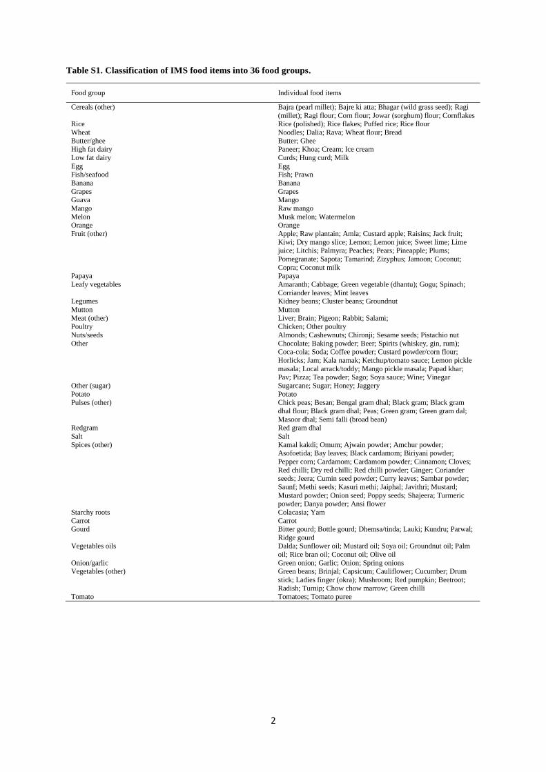
composition tables.4,5 We grouped the IMS food items into 36 food groups based on compositional similarity

(Table S1).

2

Table S1. Classification of IMS food items into 36 food groups.

Food group Individual food items

Cereals (other) Bajra (pearl millet); Bajre ki atta; Bhagar (wild grass seed); Ragi

(millet); Ragi flour; Corn flour; Jowar (sorghum) flour; Cornflakes Rice Rice (polished); Rice flakes; Puffed rice; Rice flour

Wheat Noodles; Dalia; Rava; Wheat flour; Bread

Butter/ghee Butter; Ghee High fat dairy Paneer; Khoa; Cream; Ice cream

Low fat dairy Curds; Hung curd; Milk

Egg Egg Fish/seafood Fish; Prawn

Banana Banana

Grapes Grapes Guava Mango

Mango Raw mango

Melon Musk melon; Watermelon Orange Orange

Fruit (other) Apple; Raw plantain; Amla; Custard apple; Raisins; Jack fruit;

Kiwi; Dry mango slice; Lemon; Lemon juice; Sweet lime; Lime juice; Litchis; Palmyra; Peaches; Pears; Pineapple; Plums;

Pomegranate; Sapota; Tamarind; Zizyphus; Jamoon; Coconut;

Copra; Coconut milk Papaya Papaya

Leafy vegetables Amaranth; Cabbage; Green vegetable (dhantu); Gogu; Spinach;

Corriander leaves; Mint leaves Legumes Kidney beans; Cluster beans; Groundnut

Mutton Mutton

Meat (other) Liver; Brain; Pigeon; Rabbit; Salami; Poultry Chicken; Other poultry

Nuts/seeds Almonds; Cashewnuts; Chironji; Sesame seeds; Pistachio nut

Other Chocolate; Baking powder; Beer; Spirits (whiskey, gin, rum); Coca-cola; Soda; Coffee powder; Custard powder/corn flour;

Horlicks; Jam; Kala namak; Ketchup/tomato sauce; Lemon pickle

masala; Local arrack/toddy; Mango pickle masala; Papad khar; Pav; Pizza; Tea powder; Sago; Soya sauce; Wine; Vinegar

Other (sugar) Sugarcane; Sugar; Honey; Jaggery

Potato Potato Pulses (other) Chick peas; Besan; Bengal gram dhal; Black gram; Black gram

dhal flour; Black gram dhal; Peas; Green gram; Green gram dal;

Masoor dhal; Semi falli (broad bean) Redgram Red gram dhal

Salt Salt

Spices (other) Kamal kakdi; Omum; Ajwain powder; Amchur powder; Asofoetida; Bay leaves; Black cardamom; Biriyani powder;

Pepper corn; Cardamom; Cardamom powder; Cinnamon; Cloves;

Red chilli; Dry red chilli; Red chilli powder; Ginger; Coriander seeds; Jeera; Cumin seed powder; Curry leaves; Sambar powder;

Saunf; Methi seeds; Kasuri methi; Jaiphal; Javithri; Mustard;

Mustard powder; Onion seed; Poppy seeds; Shajeera; Turmeric powder; Danya powder; Ansi flower

Starchy roots Colacasia; Yam

Carrot Carrot Gourd Bitter gourd; Bottle gourd; Dhemsa/tinda; Lauki; Kundru; Parwal;

Ridge gourd Vegetables oils Dalda; Sunflower oil; Mustard oil; Soya oil; Groundnut oil; Palm

oil; Rice bran oil; Coconut oil; Olive oil

Onion/garlic Green onion; Garlic; Onion; Spring onions Vegetables (other) Green beans; Brinjal; Capsicum; Cauliflower; Cucumber; Drum

stick; Ladies finger (okra); Mushroom; Red pumpkin; Beetroot;

Radish; Turnip; Chow chow marrow; Green chilli Tomato Tomatoes; Tomato puree

3

Distinct dietary patterns were derived using finite mixture modelling. The 36 food groups (consumption

variables) were entered into a Latent Class Analysis (LCA) model to identify distinct patterns of food

consumption based on clustering in the data.6 Solutions containing 1–10 distinct dietary patterns were specified,

and we used a combination of diagnostic criteria (Bayesian Information Criterion, minimum proportion per class

and Entropy of model) to select the solution that fitted the data best. The five-pattern model provided the best fit

to the data, and survey individuals were assigned to one of these five dietary patterns based on their probability

of inclusion in each pattern. The final patterns were expressed as average consumption in each food group in

g/capita/day. Full details of the method and the final dietary patterns can be found in other work by the authors.7

Environmental impacts of diets

Each food group was linked to data on its respective blue water footprint and GHG (CO2e) emissions as follows:

Water footprints

Crop items were matched to state level crop blue water footprints obtained from Mekonnen and Hoekstra

(2011).8 The blue water footprints of animal products were calculated following methods described in

Mekonnen and Hoekstra (2012),9 which estimates water footprints from the indirect water footprint of feed and

the direct water consumption from drinking and service water. The animal categories assessed were: beef and

dairy cattle, pig, sheep, goat, broiler and layer chicken, and the water footprint was calculated for each of

grazing, mixed and industrial systems. The ratio of different production systems for India was obtained from

work by Wint and Robinson (2007).10 The volume of feed required for each animal category was calculated

using the feed conversion efficiency and the animal product output. Feed composition was estimated from FAO

Supply and Utilisation accounts and work by Steinfeld and colleagues.11 The water footprints of the feed were

estimated using Indian state-level data on the water footprints of feed components (concentrate and roughage)

and the additional water used for mixing (blue). This was combined with drinking and service water use

(m3/animal/day), and converted to m3/tonne of product using Indian data on animal weight and yield (FAO,

2003).12 Finally, product and value fractions taken from Mekonnen and Hoekstra (2012)9 were used to convert

into consumable animal product. For prawns and fish, the water footprints were estimated using the conversion

factors per edible product,13 the total feeds used for each, and the composition of feeds for each, based on the

state-level crop data. The state-level data was then weighted by land-size using information from the Indian

census,14 and a standard error of the mean used to indicate variation for the Monte Carlo simulation (see below).

Full details of the methods used to calculate water footprints of food items are reported elsewhere.15

GHG emissions

Emissions of GHGs across the life cycle (kg CO2e/kg food) for each of the 36 food groups were derived from

published data. Where possible, India-specific data were used, but where these were not available for particular

food groups, data were extrapolated from other foods and/or countries. For each group, we combined estimates

of emissions from food production, storage, processing, transport, cooking and packaging.16–22 An additional

factor for emissions due to food waste was added, which was quantified as the product of emissions from all

other stages and the proportion of different food groups typically wasted at all stages from production to

consumption using FAO estimates for South and South East Asia.23 The GHG emissions associated with the 20

most-consumed crop and livestock products up to the production stage were estimated using a modified version

of the Cool Farm Tool,24 based on farm-level activity data for India.25 These were supplemented with emissions

for the remaining 16 food groups, as well as those for the processes from farm gate to consumer based on

previous literature.26

Dietary optimization modelling

We optimized each dietary pattern to derive new diets which (i) reduced blue water use to meet the 2025 and

2050 targets on average across the five dietary patterns and (ii) achieved World Health Organization (WHO)

nutritional guidelines for carbohydrates, fats, free sugars, protein, sodium, fruits, and vegetables (Table S2)27

with minimal deviation from existing intake (sum of squared percentage differences for all food groups) and no

change in total dietary energy.

4

Table S2. WHO nutritional guideline values.

Nutrient / food group WHO guideline

Total fat (% total energy) 15–30%

Saturated fat (% total energy) <10% Polyunsaturated fat (% total energy) 6–10%

N6 polyunsaturated fat (% total energy) 5–8%

N3 polyunsaturated fat (% total energy) 1–2% Trans fat (% total energy) <1%

Monounsaturated fat (% total energy) (remaining)

Carbohydrate (% total energy) 55–75% Free sugars (% total energy) <10%

Protein (% total energy) 10–15%

Sodium (g) <2 g Fruit and vegetables (g) ≥400 g

To achieve the overall blue water use reduction across all dietary patterns, equitable targets for each of the five

patterns were defined accounting for their baseline blue water footprints (i.e. greater levels of per capita

reduction were required for dietary patterns with higher baseline footprints). In each scenario, the method

converged per capita blue water use on the same level for each dietary pattern, though with different

contributions from each.

In the optimization, for a given food group i, the loss of welfare Wi resulting from consumption greater or less

than the ideal level for health is proportional to the share of expenditure for that food group si and inversely

proportional to the price elasticity of demand εi

∆𝑊𝑖 ∝𝑠𝑖𝜀𝑖(∆𝑋𝑖𝑋𝑖

)2

where Xi is the current consumption for food group i and ΔXi is the difference between current and ideal

consumption for food group i. The ratio of si/εi acts as a simplified measure of utility. Data on the share of

dietary expenditure (si) were taken from the nationally-representative National Sample Survey, conducted in

2004–2005.28 The survey recorded the quantity and value purchased in the last 30 days of a comprehensive list

of about 250 food and beverage items. Expenditure share for each of the 36 food groups was calculated by

dividing the value spent on a food group by total expenditure on all food. Data on price elasticities for each food

group (εi) were taken from work by Kumar and colleagues.29

The analysis then seeks to find the combination of foods that minimizes the weighted deviations of squared

percentage consumption from the desired levels, where each deviation is weighted by si/εi. For the 36 food

groups in the analysis, this can be expressed as

min{∆𝑋𝑖;𝑖=1..36}

[∑𝑠𝑖𝜀𝑖(∆𝑋𝑖𝑋𝑖

)236

𝑖=1

]

Initial estimates of optimized consumption for each food group (i.e. initial estimates of the solution of the above

equation) were generated randomly. The optimization was performed in the statistical language R30 using the

package Alabama, which uses an augmented Lagrangian method with an adaptive barrier function to optimize

nonlinear functions including constraints.31 The augmented Lagrangian method is a form of nonlinear

programming that works by replacing the (constrained) problem with a sequence of unconstrained functions that

are augmented with a penalty function. Lagrange multipliers (commonly used in mathematical optimization) are

used to find the local minima or maxima at each stage. The application of the method to dietary optimization has

been described in previous work by the authors.32,33

5

Modelling the impact on health

We estimated the impact on mortality due to adoption of each optimized dietary pattern using a life table

method adapted from the IOMLIFET model34 coded in R. The model was set up using age- and cause-specific

mortality and population data from the Indian Registrar General, United Nations and WHO projected to 2050

based on extrapolation of recent trends using second order polynomial functions.35–38

Guided by evidence from the Global Burden of Disease (GBD) study39 and a previous literature review of meta-

analyses relating food or nutrient consumption to non-communicable disease,32 we assessed the impact on health

through the effects of changes in consumption of mutton and other red meat, fruits, and vegetables (Table S3)

on the following mortality outcomes: coronary heart disease, stroke, type 2 diabetes and cancers of the

mouth/pharynx/larynx, oesophagus, lung, stomach, and colon/rectum (Table S4).

Table S3. Food groups classified as mutton and other red meat, fruits, and vegetables.

Dietary exposure Food groups

Mutton and other

red meat Mutton; Meat (other)

Fruits Banana; Grapes; Guava; Mango; Melon; Fruit (other); Orange; Papaya Vegetables Carrot; Gourd; Leafy vegetables; Onion/garlic; Vegetables (other); Tomato

Table S4. Underlying cause of death classifications (ICD-10) used for each health outcome.

Health outcome

ICD-10 underlying cause of death classification

Codes Underlying causes

Coronary heart disease I20–I25 Ischaemic heart diseases

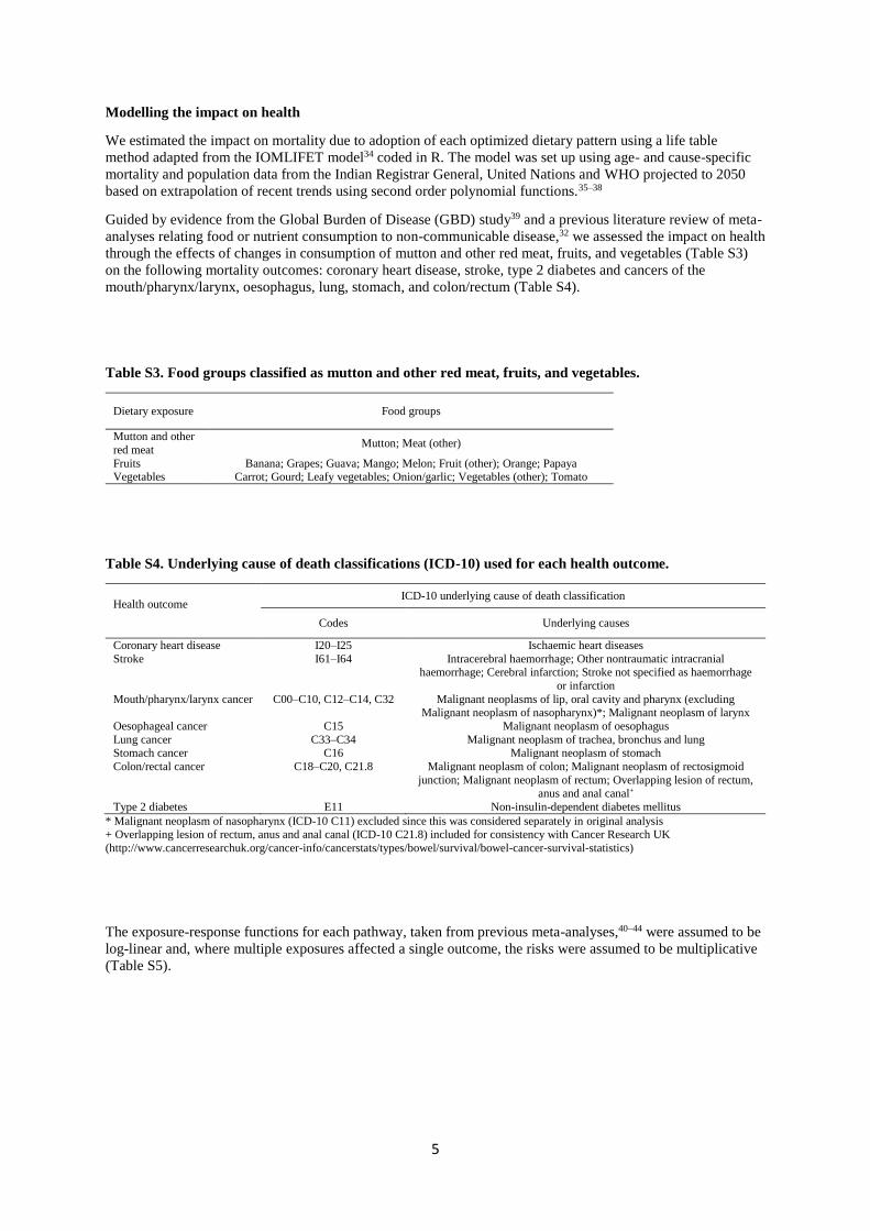
Stroke I61–I64 Intracerebral haemorrhage; Other nontraumatic intracranial haemorrhage; Cerebral infarction; Stroke not specified as haemorrhage

or infarction

Mouth/pharynx/larynx cancer C00–C10, C12–C14, C32 Malignant neoplasms of lip, oral cavity and pharynx (excluding Malignant neoplasm of nasopharynx)*; Malignant neoplasm of larynx

Oesophageal cancer C15 Malignant neoplasm of oesophagus

Lung cancer C33–C34 Malignant neoplasm of trachea, bronchus and lung Stomach cancer C16 Malignant neoplasm of stomach

Colon/rectal cancer C18–C20, C21.8 Malignant neoplasm of colon; Malignant neoplasm of rectosigmoid

junction; Malignant neoplasm of rectum; Overlapping lesion of rectum, anus and anal canal+

Type 2 diabetes E11 Non-insulin-dependent diabetes mellitus

* Malignant neoplasm of nasopharynx (ICD-10 C11) excluded since this was considered separately in original analysis + Overlapping lesion of rectum, anus and anal canal (ICD-10 C21.8) included for consistency with Cancer Research UK

(http://www.cancerresearchuk.org/cancer-info/cancerstats/types/bowel/survival/bowel-cancer-survival-statistics)

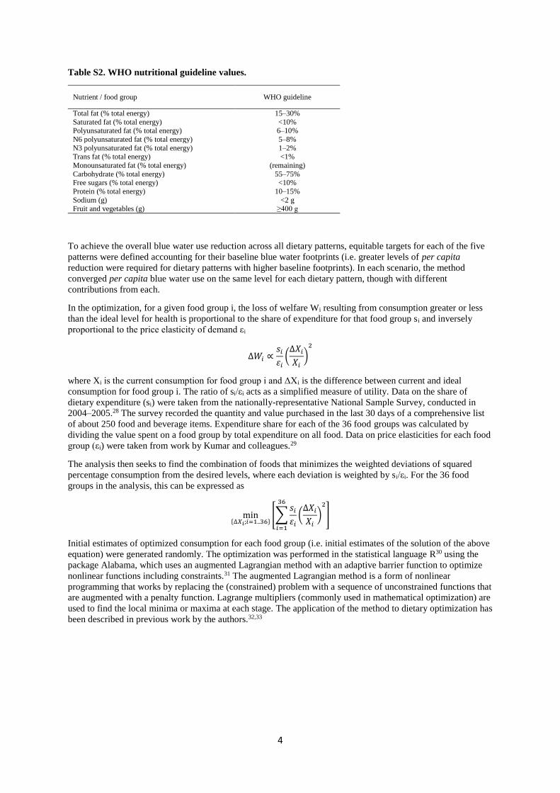
The exposure-response functions for each pathway, taken from previous meta-analyses,40–44 were assumed to be

log-linear and, where multiple exposures affected a single outcome, the risks were assumed to be multiplicative

(Table S5).

6

Table S5. Dietary exposure-response pathways used in health impact model

Dietary exposure Health outcome Relative risk (95% confidence intervals) Source

Fruit Coronary heart disease 0·93 (0·89–0·96) per 80 g increase per day Dauchet et al. (2006)40

Stroke 0·89 (0·85–0·93) per 80 g increase per day Dauchet et al. (2005)41

Mouth/pharynx/larynx cancer 0·72 (0·59–0·87) per 100 g increase per day Marmot et al. (2007)42 Oesophagus cancer 0·56 (0·42–0·74) per 100 g increase per day Marmot et al. (2007)42

Lung cancer 0·94 (0·90–0·97) per 80 g increase per day Marmot et al. (2007)42

Stomach cancer 0·67 (0·59–0·76) per 100 g increase per day Marmot et al. (2007)42 Vegetables (non-starchy) Coronary heart disease 0·89 (0·83–0·95) per 80 g increase per day Dauchet et al. (2006)40

Stroke 0·97 (0·92–1·02) per 80 g increase per day Dauchet et al. (2005)41

Mouth/pharynx/larynx cancer 0·72 (0·63–0·82) per 50 g increase per day Marmot et al. (2007)42 Oesophagus cancer 0·87 (0·72–1·05) per 50 g increase per day Marmot et al. (2007)42

Stomach cancer 0·70 (0·62–0·79) per 100 g increase per day Marmot et al. (2007)42

Mutton and other red meat

Colon/rectal cancer 1·29 (1·04–1·60) per 100 g increase per day Marmot et al. (2007)42

Type 2 diabetes 1·19 (1·04–1·37) per 100 g increase per day Pan et al. (2011)43

Stroke 1·21 (1·10–1·33) per 100 g increase per day Micha et al. (2010)44

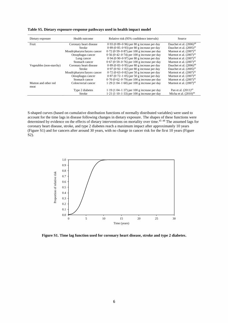
S-shaped curves (based on cumulative distribution functions of normally distributed variables) were used to

account for the time lags in disease following changes in dietary exposure. The shapes of these functions were

determined by evidence on the effects of dietary interventions on mortality over time.45–48 The assumed lags for

coronary heart disease, stroke, and type 2 diabetes reach a maximum impact after approximately 10 years

(Figure S1) and for cancers after around 30 years, with no change in cancer risk for the first 10 years (Figure

S2).

Figure S1. Time lag function used for coronary heart disease, stroke and type 2 diabetes.

0.0

0.1

0.2

0.3

0.4

0.5

0.6

0.7

0.8

0.9

1.0

0 5 10 15 20 25 30

Pro

port

ion

of

rela

tive

risk

Time (years)

7

Figure S2. Time lag function used for cancer outcomes.

Further details of the health impact model, including time lag functions, can be found in previous work by the

authors.33 The primary outcomes of the model were changes in life years lived due to each outcome over a

follow up period of 40 years (i.e. to 2050).

Monte Carlo analysis

We employed a Monte Carlo method whereby each simulation was repeated 1000 times to obtain a measure of

the uncertainties associated with our estimates. For each repetition, we sampled randomly from the distribution

of input parameters (water footprints, expenditure shares, exposure-response coefficients), assuming normal

distributions for each. For the baseline consumption in each dietary pattern, we took consumption of each food

group for each individual in the IMS data assigned to that pattern and estimated the standard deviations. For

water footprints, the level of variation was based on spatial differences in the state-level data, which were

dependent on differences in yields and climate factors. For expenditure shares, the estimates were based on the

standard errors of the survey data and, for the exposure-response coefficients, we used the 95% confidence

intervals from the original published sources. Where we were unable to obtain full information on the

uncertainties (nutritional composition, GHG emissions, price elasticities), we assumed uniform distributions of

±10% around the central estimates. To reduce the likelihood of locating local minima, within each individual

simulation the optimization process was repeated 20 times and the ‘best’ result (minimum objective value while

meeting all constraints) was selected.

0.0

0.1

0.2

0.3

0.4

0.5

0.6

0.7

0.8

0.9

1.0

0 5 10 15 20 25 30

Pro

port

ion

of

rela

tive

risk

Time (years)

8

RESULTS

Consumption in baseline and optimized dietary patterns: 2025 scenario

Figure S3. Average consumption of 36 food groups in g/day for Rice and low diversity pattern currently

(green bars) and following optimization (orange bars) under 2025 scenario. Error bars = 95% confidence

intervals.

Figure S4. Average consumption of 36 food groups in g/day for Rice and fruit pattern currently (green

bars) and following optimization (orange bars) under 2025 scenario. Error bars = 95% confidence

intervals.

9

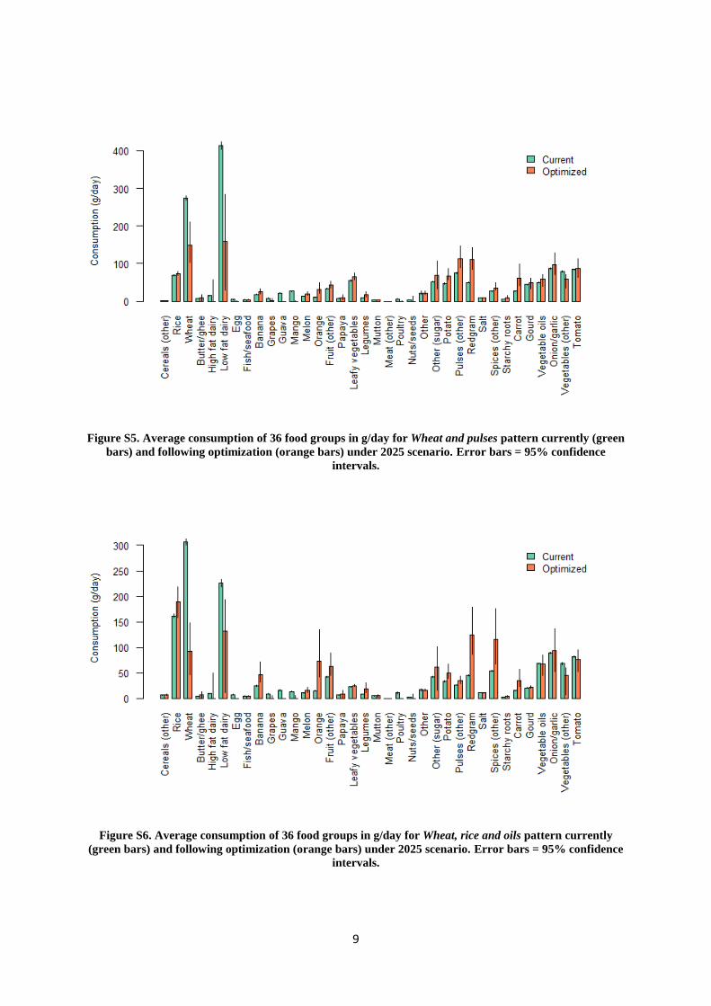
Figure S5. Average consumption of 36 food groups in g/day for Wheat and pulses pattern currently (green

bars) and following optimization (orange bars) under 2025 scenario. Error bars = 95% confidence

intervals.

Figure S6. Average consumption of 36 food groups in g/day for Wheat, rice and oils pattern currently

(green bars) and following optimization (orange bars) under 2025 scenario. Error bars = 95% confidence

intervals.

10

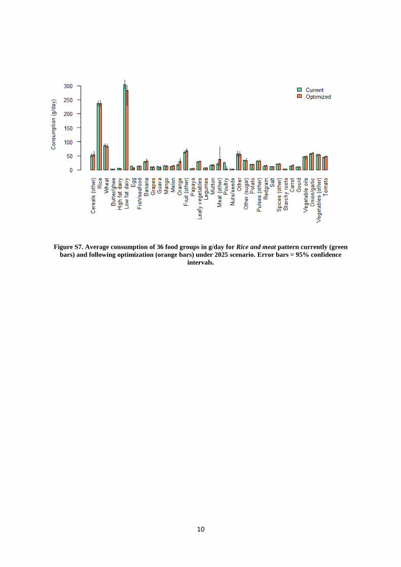
Figure S7. Average consumption of 36 food groups in g/day for Rice and meat pattern currently (green

bars) and following optimization (orange bars) under 2025 scenario. Error bars = 95% confidence

intervals.

11

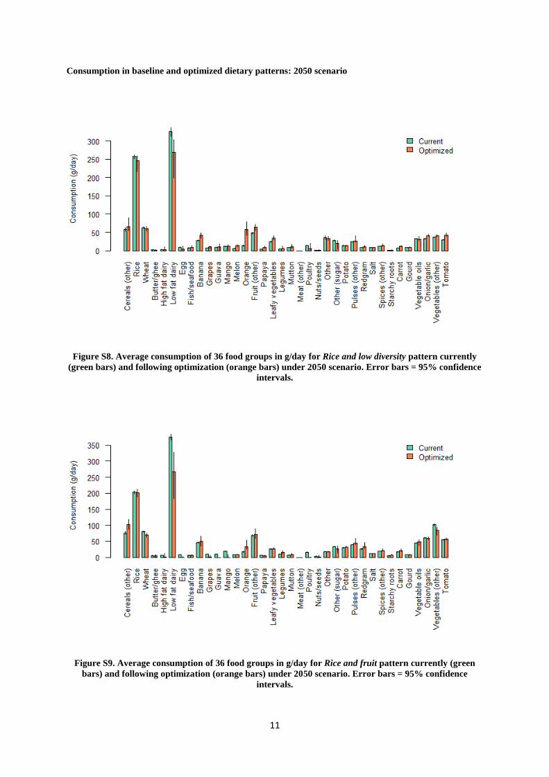
Consumption in baseline and optimized dietary patterns: 2050 scenario

Figure S8. Average consumption of 36 food groups in g/day for Rice and low diversity pattern currently

(green bars) and following optimization (orange bars) under 2050 scenario. Error bars = 95% confidence

intervals.

Figure S9. Average consumption of 36 food groups in g/day for Rice and fruit pattern currently (green

bars) and following optimization (orange bars) under 2050 scenario. Error bars = 95% confidence

intervals.

12

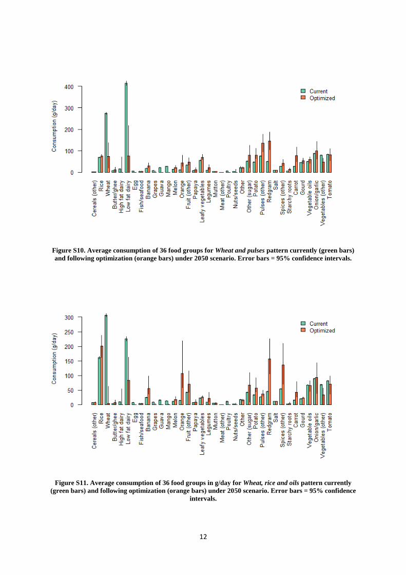
Figure S10. Average consumption of 36 food groups for Wheat and pulses pattern currently (green bars)

and following optimization (orange bars) under 2050 scenario. Error bars = 95% confidence intervals.

Figure S11. Average consumption of 36 food groups in g/day for Wheat, rice and oils pattern currently

(green bars) and following optimization (orange bars) under 2050 scenario. Error bars = 95% confidence

intervals.

13

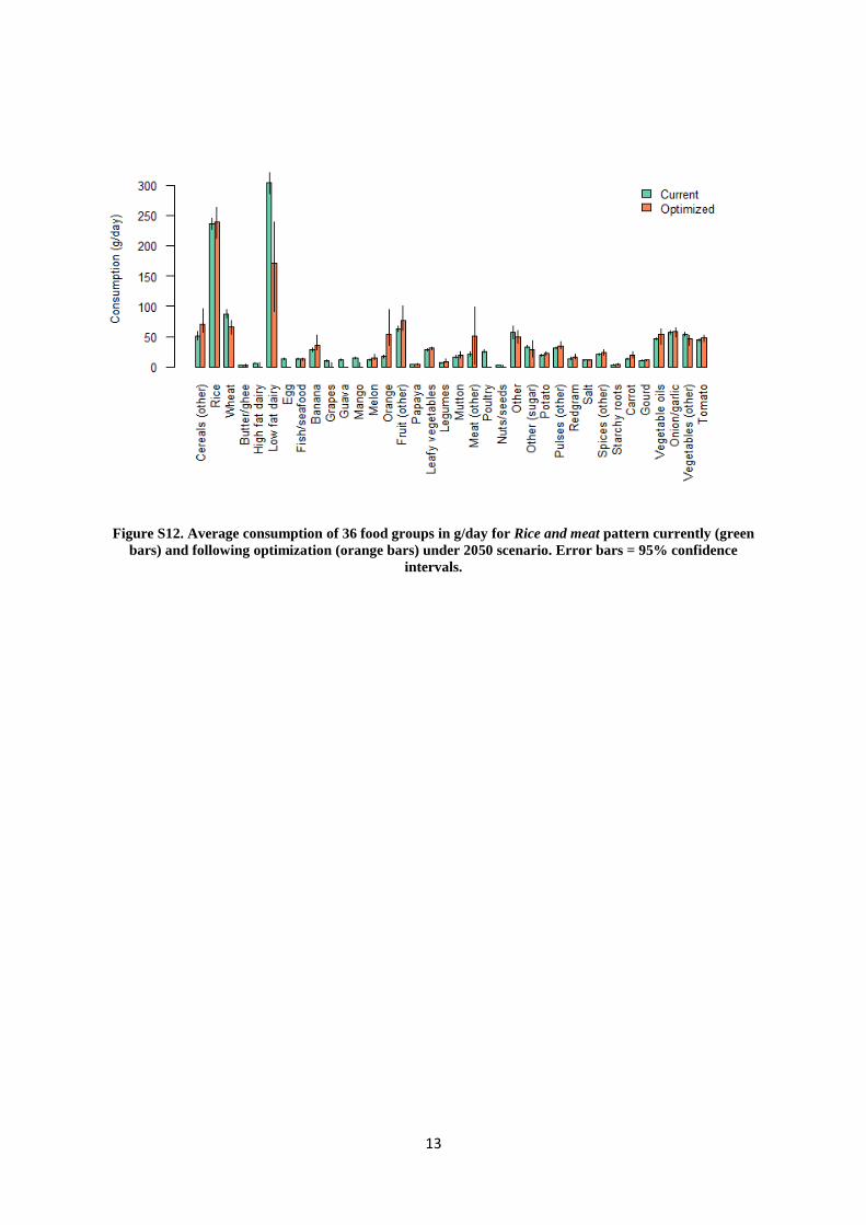
Figure S12. Average consumption of 36 food groups in g/day for Rice and meat pattern currently (green

bars) and following optimization (orange bars) under 2050 scenario. Error bars = 95% confidence

intervals.

14

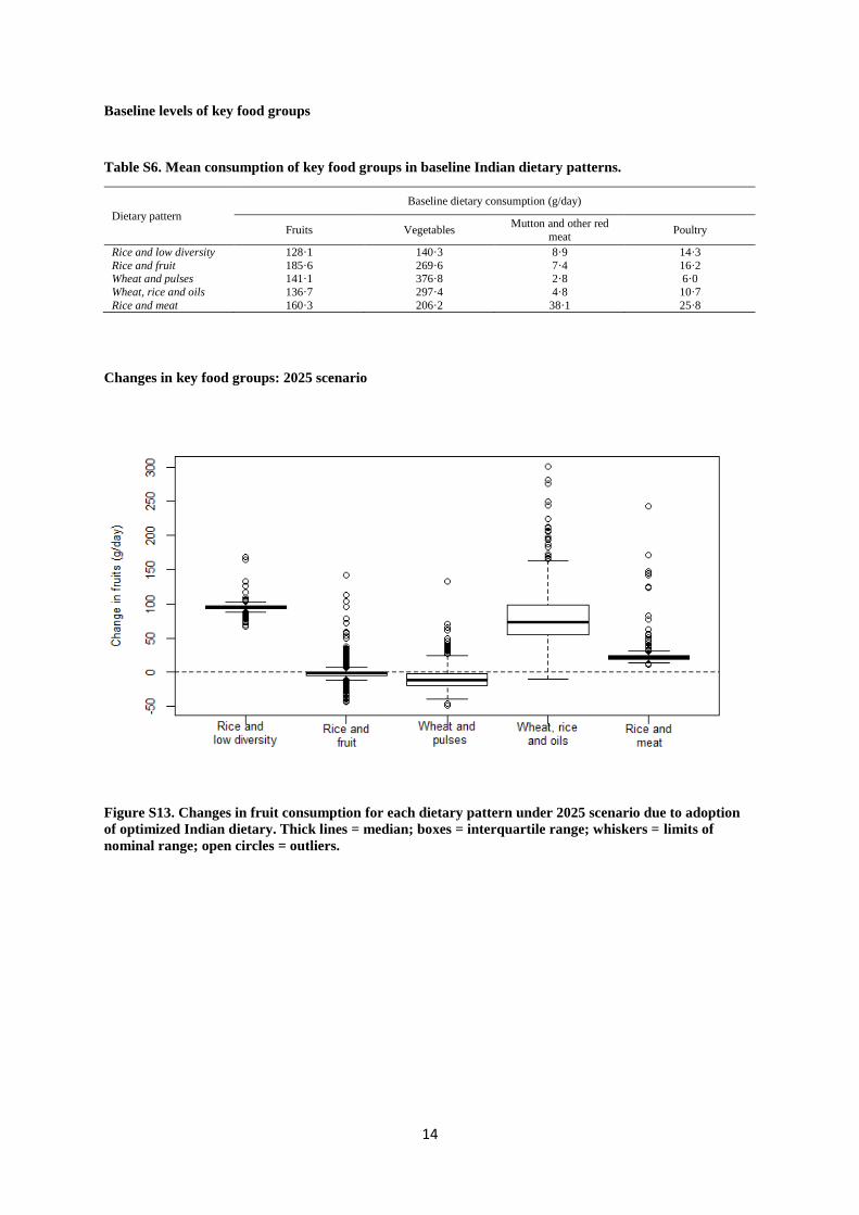
Baseline levels of key food groups

Table S6. Mean consumption of key food groups in baseline Indian dietary patterns.

Dietary pattern

Baseline dietary consumption (g/day)

Fruits Vegetables Mutton and other red

meat Poultry

Rice and low diversity 128·1 140·3 8·9 14·3

Rice and fruit 185·6 269·6 7·4 16·2 Wheat and pulses 141·1 376·8 2·8 6·0

Wheat, rice and oils 136·7 297·4 4·8 10·7

Rice and meat 160·3 206·2 38·1 25·8

Changes in key food groups: 2025 scenario

Figure S13. Changes in fruit consumption for each dietary pattern under 2025 scenario due to adoption

of optimized Indian dietary. Thick lines = median; boxes = interquartile range; whiskers = limits of

nominal range; open circles = outliers.

15

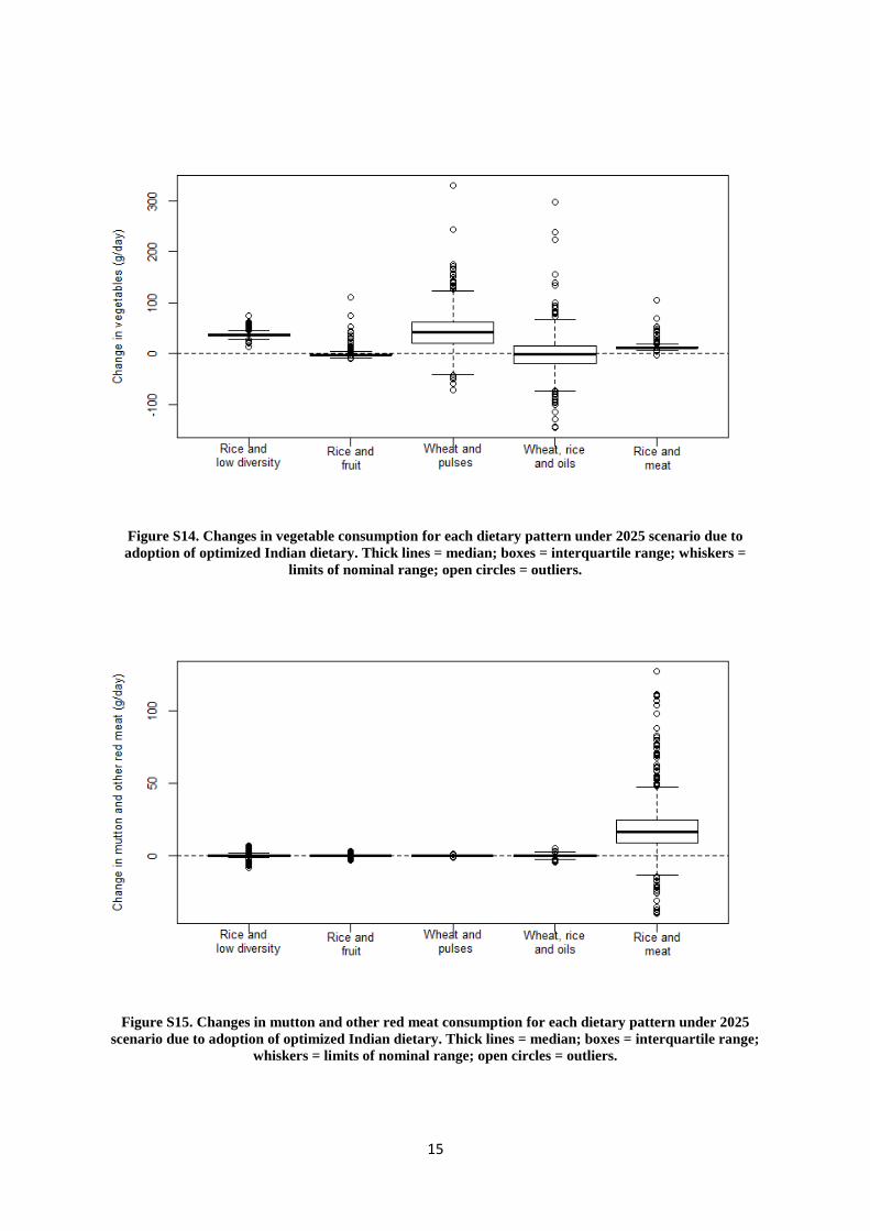
Figure S14. Changes in vegetable consumption for each dietary pattern under 2025 scenario due to

adoption of optimized Indian dietary. Thick lines = median; boxes = interquartile range; whiskers =

limits of nominal range; open circles = outliers.

Figure S15. Changes in mutton and other red meat consumption for each dietary pattern under 2025

scenario due to adoption of optimized Indian dietary. Thick lines = median; boxes = interquartile range;

whiskers = limits of nominal range; open circles = outliers.

16

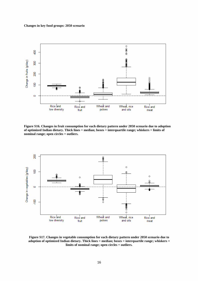
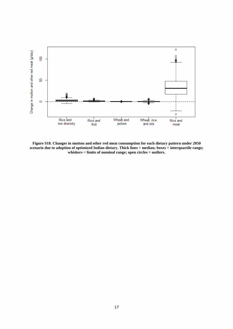
Changes in key food groups: 2050 scenario

Figure S16. Changes in fruit consumption for each dietary pattern under 2050 scenario due to adoption

of optimized Indian dietary. Thick lines = median; boxes = interquartile range; whiskers = limits of

nominal range; open circles = outliers.

Figure S17. Changes in vegetable consumption for each dietary pattern under 2050 scenario due to

adoption of optimized Indian dietary. Thick lines = median; boxes = interquartile range; whiskers =

limits of nominal range; open circles = outliers.

17

Figure S18. Changes in mutton and other red meat consumption for each dietary pattern under 2050

scenario due to adoption of optimized Indian dietary. Thick lines = median; boxes = interquartile range;

whiskers = limits of nominal range; open circles = outliers.

18

Changes in blue water footprints: 2025 scenario

Figure S19. Percentage changes in blue water footprints for each dietary pattern under 2025 scenario due

to adoption of optimized Indian dietary. Thick lines = median; boxes = interquartile range; whiskers =

limits of nominal range; open circles = outliers.

19

Changes in blue water footprints: 2050 scenario

Figure S20. Percentage changes in blue water footprints for each dietary pattern under 2050 scenario due

to adoption of optimized Indian dietary. Thick lines = median; boxes = interquartile range; whiskers =

limits of nominal range; open circles = outliers.

20

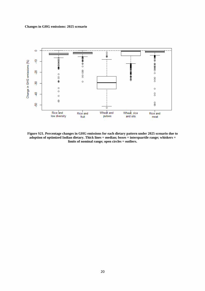
Changes in GHG emissions: 2025 scenario

Figure S21. Percentage changes in GHG emissions for each dietary pattern under 2025 scenario due to

adoption of optimized Indian dietary. Thick lines = median; boxes = interquartile range; whiskers =

limits of nominal range; open circles = outliers.

21

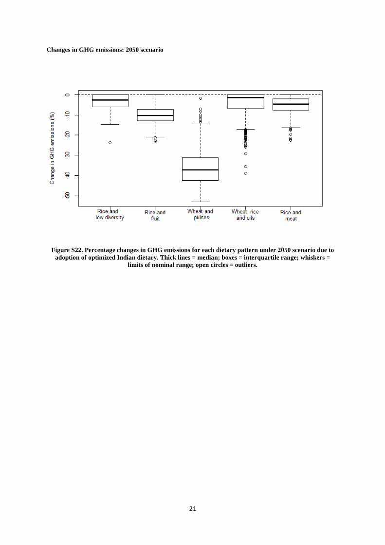
Changes in GHG emissions: 2050 scenario

Figure S22. Percentage changes in GHG emissions for each dietary pattern under 2050 scenario due to

adoption of optimized Indian dietary. Thick lines = median; boxes = interquartile range; whiskers =

limits of nominal range; open circles = outliers.

22

Health impacts

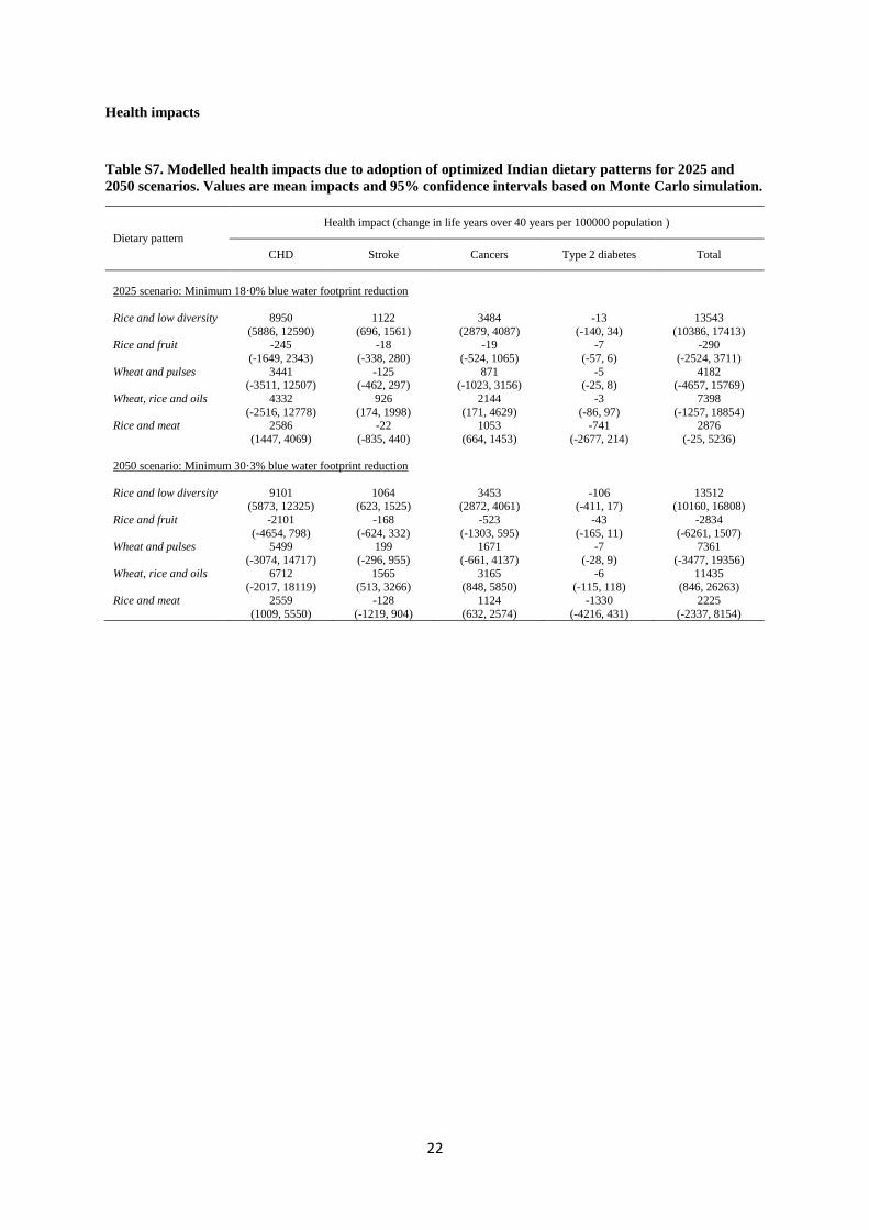
Table S7. Modelled health impacts due to adoption of optimized Indian dietary patterns for 2025 and

2050 scenarios. Values are mean impacts and 95% confidence intervals based on Monte Carlo simulation.

Dietary pattern

Health impact (change in life years over 40 years per 100000 population )

CHD Stroke Cancers Type 2 diabetes Total

2025 scenario: Minimum 18·0% blue water footprint reduction

Rice and low diversity 8950

(5886, 12590)

1122

(696, 1561)

3484

(2879, 4087)

-13

(-140, 34)

13543

(10386, 17413) Rice and fruit -245

(-1649, 2343)

-18

(-338, 280)

-19

(-524, 1065)

-7

(-57, 6)

-290

(-2524, 3711)

Wheat and pulses 3441 (-3511, 12507)

-125 (-462, 297)

871 (-1023, 3156)

-5 (-25, 8)

4182 (-4657, 15769)

Wheat, rice and oils 4332

(-2516, 12778)

926

(174, 1998)

2144

(171, 4629)

-3

(-86, 97)

7398

(-1257, 18854) Rice and meat 2586

(1447, 4069)

-22

(-835, 440)

1053

(664, 1453)

-741

(-2677, 214)

2876

(-25, 5236)

2050 scenario: Minimum 30·3% blue water footprint reduction

Rice and low diversity 9101 (5873, 12325)

1064 (623, 1525)

3453 (2872, 4061)

-106 (-411, 17)

13512 (10160, 16808)

Rice and fruit -2101

(-4654, 798)

-168

(-624, 332)

-523

(-1303, 595)

-43

(-165, 11)

-2834

(-6261, 1507) Wheat and pulses 5499

(-3074, 14717)

199

(-296, 955)

1671

(-661, 4137)

-7

(-28, 9)

7361

(-3477, 19356)

Wheat, rice and oils 6712 (-2017, 18119)

1565 (513, 3266)

3165 (848, 5850)

-6 (-115, 118)

11435 (846, 26263)

Rice and meat 2559

(1009, 5550)

-128

(-1219, 904)

1124

(632, 2574)

-1330

(-4216, 431)

2225

(-2337, 8154)

23

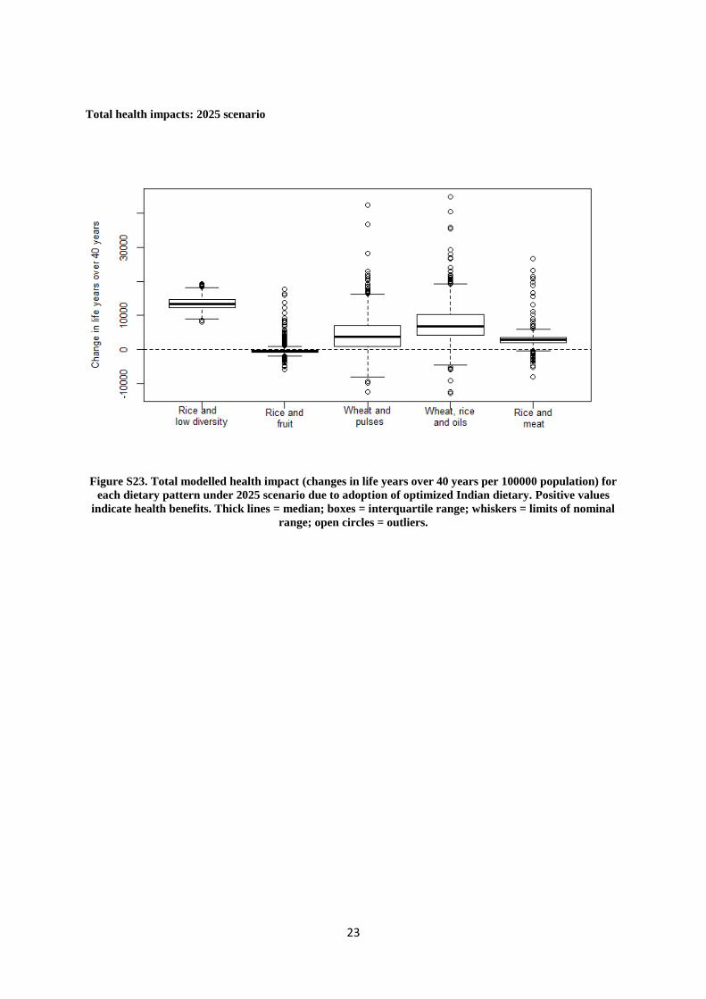
Total health impacts: 2025 scenario

Figure S23. Total modelled health impact (changes in life years over 40 years per 100000 population) for

each dietary pattern under 2025 scenario due to adoption of optimized Indian dietary. Positive values

indicate health benefits. Thick lines = median; boxes = interquartile range; whiskers = limits of nominal

range; open circles = outliers.

24

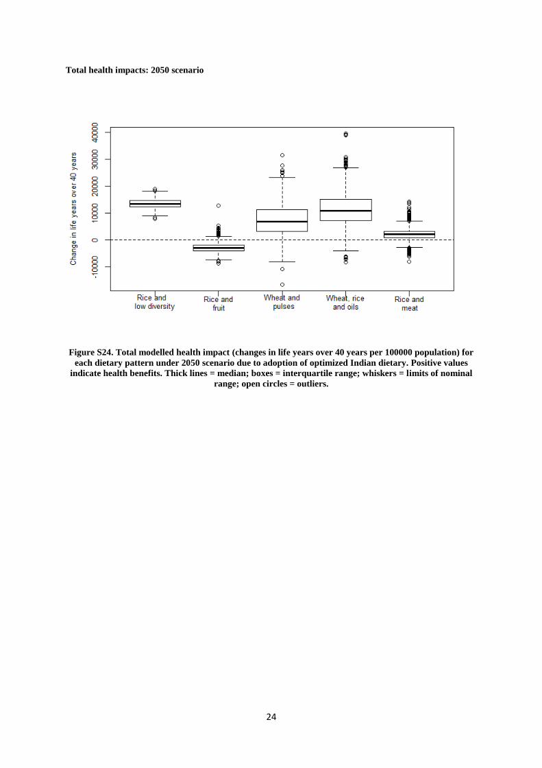
Total health impacts: 2050 scenario

Figure S24. Total modelled health impact (changes in life years over 40 years per 100000 population) for

each dietary pattern under 2050 scenario due to adoption of optimized Indian dietary. Positive values

indicate health benefits. Thick lines = median; boxes = interquartile range; whiskers = limits of nominal

range; open circles = outliers.

25

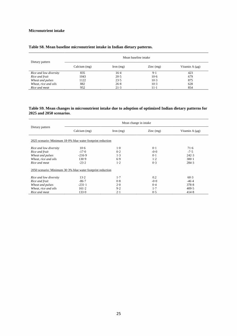
Micronutrient intake

Table S8. Mean baseline micronutrient intake in Indian dietary patterns.

Dietary pattern

Mean baseline intake

Calcium (mg) Iron (mg) Zinc (mg) Vitamin A (µg)

Rice and low diversity 835 16·4 9·1 423

Rice and fruit 1043 20·5 10·6 679

Wheat and pulses 1122 23·5 10·3 875 Wheat, rice and oils 882 26·8 10·3 628

Rice and meat 952 21·3 11·1 854

Table S9. Mean changes in micronutrient intake due to adoption of optimized Indian dietary patterns for

2025 and 2050 scenarios.

Dietary pattern

Mean change in intake

Calcium (mg) Iron (mg) Zinc (mg) Vitamin A (µg)

2025 scenario: Minimum 18·0% blue water footprint reduction

Rice and low diversity 10·6 1·0 0·1 71·6

Rice and fruit -17·0 0·2 -0·0 -7·5 Wheat and pulses -216·9 1·3 0·1 242·3

Wheat, rice and oils 130·9 6·9 1·2 300·1

Rice and meat -23·2 1·2 0·3 284·3

2050 scenario: Minimum 30·3% blue water footprint reduction

Rice and low diversity 13·2 1·7 0.2 60·3

Rice and fruit -86·7 0·8 -0·0 -46·4

Wheat and pulses -231·1 2·0 0·4 378·8

Wheat, rice and oils 161·2 9·2 1·7 409·5

Rice and meat 133·0 2·1 0·5 414·8

26

References

1 Indian Ministry of Water Resources. Strategic Plan for Ministry of Water Resources. New Delhi: Indian

Ministry of Water Resources, 2011.

2 Ebrahim S, Kinra S, Bowen L, et al. The effect of rural-to-urban migration on obesity and diabetes in India:

a cross-sectional study. PLOS Med 2010; 7: e1000268.

3 Bowen L, Bharathi AV, Kinra S, Destavola B, Ness A, Ebrahim S. Development and evaluation of a semi-

quantitative food frequency questionnaire for use in urban and rural India. Asia Pac J Clin Nutr 2012; 21:

355–60.

4 Gopalan C, Rama Sastri BV, Balasubramanian SC. Nutritive Value of Indian Foods. Hyderabad: National

Institute of Nutrition, Indian Council of Medical Research, 1971.

5 USDA-ARS. National Nutrient Database for Standard Reference, Release 28. US Department of

Agriculture, Agricultural Research Service. Available at: http://www.ars.usda.gov/nea/bhnrc/ndl

6 Fahey MT, Thane CW, Bramwell GD, Coward WA. Conditional Gaussian mixture modelling for dietary

pattern analysis. J R Stat Soc Ser A 2007; 170: 149–66.

7 Joy EJM, Green R, Agrawal S, et al. Dietary patterns and non-communicable disease risk in Indian adults:

secondary analysis of Indian Migration Study data. Public Health Nutr 2017, Submitted.

8 Mekonnen MM, Hoekstra AY. The green, blue and grey water footprint of crops and derived crop products.

Hydrol Earth Syst Sci 2011; 15: 1577–600.

9 Mekonnen MM, Hoekstra AY. A global assessment of the water footprint of farm animal products.

Ecosystems 2012; 15: 401–15.

10 Wint GRW, Robinson TP. Gridded Livestock of the World 2007. Rome: Food and Agriculture Organization

(FAO), 2007. http;//www.fao.org/docrep/010/a1259e/a1259e00.html

11 Steinfeld H, Gerber P, Wassenaar T, Castel V, Rosales M, de Haan C. Livestock’s Long Shadow:

Environmental Issues and Options. Rome: Food and Agriculture Organization (FAO), 2006.

ftp://ftp.fao.org/docrep/fao/010/a0701e/A0701E.pdf

12 FAO. Technical Conversion Factors for Agricultural Commodities. Rome: Food and Agriculture

Organization (FAO), 2003. http://www.fao.org/fileadmin/templates/ess/documents/methodology/tcf.pdf

13 Suresh AV. Development of the Aquafeed Industry in India. FAO Fisheries Technical Paper No. 497.

Rome: Food and Agriculture Organization (FAO), 2007. http://www.fao.org/3/a-a1444e/a1444e08.pdf

14 Office of the Registrar General. Census of India. New Delhi, India: Ministry of Home Affairs, Government

of India, 2011. Available at: http://www.censusindia.gov.in/2011census/hlo/pca/pca_pdf/PCA-CRC-

0000.pdf

15 Harris F, Green RF, Joy EJM, Kayatz B, Haines A, Dangour AD. The water use of Indian diets and socio-

demographic factors related to dietary blue water footprint. Sci Total Environ 2017, Accepted for

publication.

16 Foster C, Green K, Bleda M, et al. Environmental Impacts of Food Production and Consumption.

Manchester Business School, Manchester: Final Report to the Department for Environment, Food and Rural

Affairs (DEFRA), 2006.

17 Audsley E, Brander M, Chatterton J, Murphy-Bokern D, Webster C, Williams A. How Low Can We Go?

An Assessment of Greenhouse Gas Emissions from the UK Food System and the Scope for Reduction by

2050. WWF-UK, 2009.

18 FAO. Global Food Losses and Food Waste: Extent, Causes and Prevention. Rome: Food and Agriculture

Organization (FAO), 2011. http://www.fao.org/docrep/014/mb060e/mb060e.pdf

19 Pathak H, Jain N, Bhatia A, Patel J, Aggarwal PK. Carbon footprints of Indian food items. Agric Ecosyst

Environ 2010; 139: 66–73.

20 Klenk I, Landquist B, Ruiz de Imana O. The product carbon footprint of EU beet sugar: summary of key

findings. Sugar Industry Journal 2012; 137: 1–17.

21 Williams AG, Audsley E, Sandars DL. Determining the Environmental Burdens and Resource Use in the

Production of Agricultural and Horticultural Commodities. Report to the Department for Environment,

Food and Rural Affairs (DEFRA), 2006.

22 Röös E, Karlsson H, Witthoft C, Sundberg C. Evaluating the sustainability of diets – combining

environmental and nutritional aspects. Environ Sci Policy 2015; 57: 157–66.

23 FAO. FAOSTAT Food Balance Sheets. Rome: Food and Agriculture Organization (FAO), 2016.

http://faostat3.fao.org/

24 Hillier JG, Walter C, Malin D, Garcia-Suarez T, Mila-i-Canals L, Smith, P. A farm-focused calculator for

emissions from crop and livestock production. Environ Model Softw 2011; 26; 1070–8.

25 Vetter SH, Sapkota TB, Hillier J, et al. Greenhouse gas emissions from agricultural food production to

supply Indian diets: Implications for climate change mitigation. Agric Ecosyst Environ 2017, Accepted for

publication.

27

26 Green RF, Joy EJM, Harris F, et al. Greenhouse gas emissions and water footprints of typical dietary

patterns in India: a modelling study. J Clean Prod 2017, Submitted.

27 WHO. Diet, Nutrition, and the Prevention of Chronic Disease: Report of a Joint WHO/FAO Expert

Consultation. Geneva, Switzerland: World Health Organization, 2003.

28 National Sample Survey Office. Nutritional Intake in India, 2004-05. NSS 61st Round. New Delhi, India:

Government of India, 2007.

29 Kumar P, Kumar A, Parappurathu S, Raju SS. Estimation of demand elasticity for food commodities in

India. Agricultural Economics Research Review 2011; 24: 1–4.

30 R Core Team. R: A language and environment for statistical computing. Contract No.: ISBN 3-900051-07-

0 http://www.R-project.org/. Vienna, Austria: R Foundation for Statistical Computing.

31 Varadhan R. Alabama: Constrained Nonlinear Optimization. R Package Version 2011.9-1, 2012.

http://CRAN.Rproject.org/package=Alabama

32 Green R, Milner J, Dangour AD, et al. The potential to reduce greenhouse gas emissions in the UK through

healthy and realistic dietary change. Clim Change 2015; 129: 253–65.

33 Milner J, Green R, Dangour AD, et al. Health effects of adopting low greenhouse gas emission diets in the

UK. BMJ Open 2015; 5: e007364.

34 Miller B, Hurley J. Life table methods for quantitative impact assessments in chronic mortality. J Epidemiol

Community Health 2003; 57: 200–6.

35 Office of the Registrar General. Report of Causes of Death in India 2001-2003. New Delhi, India: Ministry

of Home Affairs, Government of India, 2009.

36 Office of the Registrar General. Report of Medical Certification of Cause of Death 2012. New Delhi, India:

Ministry of Home Affairs, Government of India, 2015.

37 UNSD. UNdata website. New York, NY, USA: United Nations Statistics Division, 2015.

http://data.un.org/Default.aspx

38 WHO. Global Health Observatory website. Geneva, Switzerland: World Health Organization, 2015.

http://www.who.int/gho/en/

39 Vos T, Barber RM, Bell B, et al. Global, regional, and national incidence, prevalence, and years lived with

disability for 301 acute and chronic diseases and injuries in 188 countries, 1990–2013: a systematic analysis

for the Global Burden of Disease Study 2013. Lancet 2015; 386: 743–800.

40 Dauchet L, Amouyel P, Dallongeville J. Fruit and vegetable consumption and risk of stroke: a meta-

analysis of cohort studies. Neurology 2005; 65: 1193–7.

41 Dauchet L, Amouyel P, Hercberg S, Dallongeville J. Fruit and vegetable consumption and risk of coronary

heart disease: A meta-analysis of cohort studies. J Nutr 2006; 136: 2588–93.

42 Marmot M, Atinmo T, Byers T, et al. Food, nutrition, physical activity, and the prevention of cancer: a

global perspective. World Cancer Res Fund/Am Inst Cancer 2007; 46: 312–14.

43 Pan A, Sun Q, Bernstein AM, et al. Red meat consumption and risk of type 2 diabetes: 3 cohorts of US

adults and an updated meta-analysis. Am J Clin Nutr 2011; 94: 1088–96.

44 Micha R, Wallace SK, Mozaffarian D. Red and processed meat consumption and risk of incident coronary

heart disease, stroke and diabetes mellitus - a systematic review. Circulation 2010; 121: 2271-83.

45 Capewell S, O'Flaherty M. Can dietary changes rapidly decrease cardiovascular mortality rates? Eur Heart

J 2011; 32: 1187–9.

46 Franco M, Ordunez P, Caballero B, et al. Impact of energy intake, physical activity, and population-wide

weight loss on cardiovascular disease and diabetes mortality in Cuba, 1980-2005. Am J Epidemiol 2007;

166: 1377–80.

47 Harashima E, Nakagawa Y, Urata G, Tsuji T, Shirataka M, Matsumura Y. Time-lag estimate between

dietary intake and breast cancer mortality in Japan. Asia Pac J Clin Nutr 2007; 16: 193–8.

48 Tsuji K, Harashima E, Nakagawa Y, Urata G, Shirataka M. Time-lag effects of dietary fiber and fat intake

ratio on Japanese colon cancer mortality. Biomed Environ Sci 1996; 9: 223–8.